Six Sigma Process Capability Analysis When the …...Six Sigma Process Capability Analysis When the...

Workshop on Lean Six Sigma, Smart manufacturing and Lean Systems Research Group, Lawrence Technological University, March 26, 2014

1

Six Sigma Process Capability Analysis When the Process Measurements do not follow a Normal Distribution: A Case Study

Amar Sahay, Ph.D.* Professor, Operations and Supply Chain Mgt.

BB107 R, 4600 So. Redwood Road Salt Lake City, UT 84123 USA

* Affiliation: School of Business and Technology, Salt Lake Comm. College/QMS Global LLC [email protected]

Karun Mehta

Senior Research Engineer QMS Global LLC

6990 South 300 West #321 Sandy, UTAH

(801) 957-5767 www.realleansixsigmaquality.com

Abstract

Most Six Sigma process capability analyses are based on the assumption that the process data are normally distributed. However, many processes, particularly those involving life and reliability data, do not follow normal distribution. Evaluating Process Capability using the assumptions of normality in such cases may lead to erroneous evaluation and wrong conclusions. In cases, where the process measurements do not follow a normal distribution, special techniques are required to deal with non-normality. This paper examines the evaluation techniques for non-normal process data, and provides cases and analysis techniques for such data. In the first part of the paper, the probability plot is used to fit an appropriate distribution. Then that distribution is used to determine the nonconformance rate or the process capability. In the second part of the paper, the following non-normal process capability techniques are used to evaluate non-normal data: (1) the distribution fit approach, (2) Box-Cox Transformation, and (3) Johnson Transformation. These methods provided almost identical process capability for the same data. The paper also examined the most common methods for handling non-normal data including sub group averaging, segmenting data, transforming data, using other distributions (Wiebull Distributions, Log Normal, Exponential, Extreme value , and Logistic), and using the non-parametric methods. Determining the correct process capability in Six Sigma is critical to assessing the current and improved process performance of any process. During a Six Sigma project, the process capability is evaluated twice; first during the measure phase to show the impact of the problem and again after the improvement phase to show how the process has improved. This paper addresses the importance and evaluation techniques of process capability involving non-normal data. Keywords: Process Capability Analysis, Six Sigma, Data Transformation, Non-normality.


2

Topic area of submission: Industrial/Manufacturing Engineering and Quality Engineering & Management Presentation Format: Research Paper 1.0 Introduction Process Capability is the ability of the process to meet specifications. It determines how the specifications for the product compare with the inherent variability in a process. The inherent variability of the process is the part of process variation due to common causes (the other type of process variability may be due to special causes of variation). It is a common practice to take 6 spread of a process’s inherent variation as a measure of process capability when the process is stable. Thus, the process spread is the process capability, which is equal to 6. Process Capability Analysis is an important part of overall quality improvement program. Process capability analysis is done to assess the ability of the process. It involves using the statistical techniques in the product development phase, assessing and quantifying variability before and after the product is released for production, analyzing the variability relative to product specifications, and improving product development and manufacturing process to reduce the variability. Variation reduction is the key to product improvement and product consistency. The process capability analysis is useful in: determining how well the process will hold the tolerances (the difference between specifications), selecting or modifying the process during product design and development, selecting the vendors, assessing the process requirements for machines and equipments, and above all, reducing the variability in the process. 2.0 Determining Process Capability

Process capability is assessed once the process has attained statistical control. This

means that the special causes of variation have been identified and eliminated. Once the process is stable, the process average and standard deviation are calculated. For a process that is out of control, the estimated process average and standard deviation are not reliable.

In calculating process capability, in most cases, the specification limits are required. Since the process capability determines the ability of the process to meet the specifications, it is very important to determine the specification limits accurately. Unrealistic or inaccurate specification limits may not provide correct process capability.

Determining the process capability using a histogram or a control chart is based on the assumption that the process characteristics follow a normal distribution. While the assumption of normality holds in many such situations, there are cases where the processes do not follow a normal distribution. Extreme care should be exercised in cases where normality does not hold. In cases where the data are not normal, it is important to determine the appropriate distribution or transformation techniques to perform process capability. This paper deals with process capability analysis for non-normal data.


3

3.0 Non-Normal Data Many processes do not follow normal distribution. Some examples of non-normal data would be component life data, reliability, cycle time data, customer waiting time, or number of calls arriving. Evaluating Process Capability using the assumptions of normality in such cases may lead to erroneous evaluation and wrong conclusions. In cases, where the process measurements do not follow a normal distribution, special techniques are required to deal with non-normality. A simple example is shown below. The example demonstrates that using the correct distribution is critical to determining the process capability. Since the process capability is the ability of the process to meet specifications, the situation described below determines the nonconformance rate or the percentage outside of the specification limit. 4.0 Estimating the Process Capability (percentage nonconforming) using correct Distribution Figure 1 shows the life of certain type of electronic chip. Suppose that the process producing the chips is in statistical control so that the process capability can be determined. It is required to calculate the capability with a lower limit because the company making the chips wants to know the minimum survival rate. They want to determine the percentage surviving 150 hours or less.

Life in Hrs

Freq

uenc

y

2250180013509004500-450

40

30

20

10

0

Mean 494.1StDev 484.9N 150

Histogram of Life in HrsNormal

Life in Hrs

Freq

uenc

y

2250180013509004500

50

40

30

20

10

0

Mean 494.1N 150

Exponential Histogram of Life Data with Fitted Curve

Figure 1: Life of Electronic Chip Figure 2: Exponential Distribution Fitted to the Data Figure 1 clearly indicates that the data is not normal. Therefore, it will lead to wrong conclusion if we use the normal distribution to calculate the nonconformance rate. It seems reasonable to assume that the life data might follow an exponential distribution. Therefore, the exponential distribution was fitted to the data to estimate the parameters of the distribution. The histogram with a fitted exponential curve is shown in Figure 2. The exponential distribution seems to provide a good fit to the data. The parameter of the exponential distribution (mean =494.1 hrs) is also estimated on the plot.

In Figure 3, two probability plots of the Life data are shown, one with the normal distribution and the other using the exponential distribution. The plot using the exponential distribution clearly fits the data as most of the plotted points are along the straight line. Once the correct distribution has been identified, the nonconformance rate can be determined. Recall that we want to determine the probability or the percentage of the bulbs that last 150 hours or less. Using exponential distribution with the estimated mean (shown on the probability plot and in Figure 2) of 494.1 hours, the nonconformance rate is shown in Table 1.

(a) (b) Figure 3: Probability Plots of the Life Data

Table 2

Cumulative Distribution Function Exponential with mean = 494.1 x P( X <= x ) 150 0.261831

The table shows that the probability, P (x 150) = 0.2618 or 26.18% of the products will fail within 150 hours or less. Suppose a normal distribution is used to calculate this percentage. Using the estimated mean and standard deviation (494.1 and 484.9 respectively) on the probability plot in Figure 3(a), this probability is 23.9%. The above case demonstrated how process capability could be assessed by calculating the percentage of the products outside of the specification limits or by calculating the nonconformance rate. It also emphasized on using the correct distribution in determining the process capability. If the data are not normal, it is important to determine and use the correct distribution to calculate the process capability. Many computer software can fit distributions to the data and produce probability plots based on these distributions. However, the probability plots are subjective and may lead to different conclusions. In some cases, the experience and the knowledge of the process is helpful in determining the correct distribution.

Life in Hrs

Pe

rce

nt

3000200010000-1000

99.9

99

9590

80706050403020

10

5

1

0.1

Mean

<0.005

494.1StDev 484.9N 150AD 7.566P-Value

Probability Plot of Life in HrsNormal

Life in Hrs

Pe

rce

nt

100001000100101

99.999

9080706050403020

10

5

32

1

0.1

Mean 494.1N 150AD 0.201P-Value 0.954

Probability Plot of Life in HrsExponential


5

5.0 Other ways of Dealing with Non-normal Data If the process data are not normal, other analysis methods must be employed to deal with non-normality. Some of the methods of dealing with non-normal data include using the distribution fit, transforming the data to normality, sub group averaging, segmenting data, and using non-parametric statistics. When the data are not normal, an appropriate distribution fitting the data can be selected. Knowledge of the process may be helpful in identifying the correct distribution. The commonly used distributions are Weibull, exponential, non-normal, extreme value, logistics, or log logistics. Once the correct distribution is identified, that particular distribution is then used to assess the process capability. Probability plots using computer software are very helpful in this case. Transformation such as, the Box Cox transformation, Johnson’s transformation, and others can be used to transform the non-normal data to a normal data. Once the data are brought to normality, the usual methods of normal distribution can be used to assess the process capability. It is important to note here that the transformations do not always provide consistent results. The other method of dealing with non-normal data is sub group averaging. The sub grouping is often used with the control charts where the average of sub group size greater than 4 produces a normal data. The sub group averaging is based on the concept of central limit theorem. In this method, the more skewed the data, the more samples are needed. Segmenting data and Non-parametric statistics are other methods of dealing with non-normal data. In data segmentation, data sets are segmented into smaller groups by stratification. These groups can then be examined for normality. The segmented data can often become groups of normal data. When no valid assumptions about the data can be made, non-parametric methods are used. In this paper, we have examined the following three methods to assess the process capability.

(1) Distribution-fit approach, (2) Box Cox transformation, and (3) Johnson’s transformation.

We assessed the process capability of non-normal data using the three methods above and compared the results. We found that the distribution fit and the transformation methods could produce identical results. 6.0 Process capability analysis of non-normal data The data in Table 2 shows the time to failure of high-brightness monochrome picture tubes of a projection television produced by the manufacturer of a big screen TV. The mean time to failure is estimated to be 1800 days (approximately 5 years). The manufacturer provides replacement guarantees if the failure occurs within the first 6 months or 180 days. Based on this data, the manufacturer wants to determine the number of tubes that will experience failure during the first six months of use. They also want to determine the number of tubes that have a life of 10 years (3650 days) or more. In other words, the manufacturer wants to determine the capability of the picture tube manufacturing process with LSL = 180 days and USL = 3650 days.


6

The process capability analysis of this data using the three methods is discussed below.

Table 2: Life of Monochrome Picture Tube 682 1321 5098 737 3080 1281 156 1 5672 2269 146 203 7493 247 2095 597 3796 284 2772 4977 821 483 7733 145 4082 1312 1240 261 3746 2085 577 2434 261 252 2800 367 3678 332 169 73 482 229 2899 2866 1191 1990 62 931 61 364 2685 344 5083 1572 1683 3866 4190 331 2653 2500 1536 167 616 1225 827 1881 802 342 3246 983 1846 288 3252 378 846 3097 4781 516 416 888 2359 972 113 1243 1376 1495 1464 2255 142 3088 1319 1246 1564 2588 828 1032 4663 239 5774 1090 330 1026 1212 3839 825 863 2418 488 474 263 634 3241 21 2916 374 4491 1636 830 770 935 369 1890 534 2122 2779

6.1 Process Capability using Distribution Fit Approach (Method 1) In this case, the appropriate method is to fit an appropriate distribution and use that distribution, rather than the normal distribution, to determine the process capability. The distribution-fit using probability plots were used for this case. The most appropriate distribution was identified for the data. Next, the fitted distribution was used to determine the process capability. Figure 4 shows the plot of the life data in Table 2. The distribution is clearly non-normal.

Life

Freq

uenc

y

750060004500300015000

40

30

20

10

0

Histogram of Life of Monochrome Picture Tube

Figure 4: Plot of the Data in Table 2 6.1.1 Fitting the Distribution to the Data: The distribution-fit approach was used to identify the most appropriate distribution for the data. Figure 5 shows the probability plots produced as a result of fitting some selected distributions. The appropriate distribution can be identified using the probability plots in Figure 5 and the information about the Anderson-Darling (AD) statistics, the corresponding p-values for each distribution selected, the descriptive statistics, goodness-of-fit results, and distribution parameters. In our case, more than one distribution seemed to fit the data. In such a case, use the one with the largest p-


7

value or, use the distribution that you have used before for the same or similar data. Experience and the knowledge of the process are helpful. For our data, the largest p-value, p=0.709 is for the Exponential distribution. We conclude that the failure data follow an Exponential distribution. Using this distribution, the process capability for this process was determined with LSL = 180 days and USL = 3650 days. The results are in Figure 6.

Life of M onochrome P ictur e T ube

Pe

rce

nt

50000-5000

99.999

90

50

10

1

0.1


Pe

rce

nt

100001000100101

99.990

50

10

1

0.1


Pe

rce

nt

100001000100101

99.9

90

50

10

1

0.1


Pe

rce

nt

10000.01000.0100.010.01.00.1

99.99990

50

10

1

0.1

Goodness of F it Test

P -V alue > 0.250

GammaA D = 0.358 P -V alue > 0.250

NormalA D = 5.506 P -V alue < 0.005

ExponentialA D = 0.364 P -V alue = 0.709

WeibullA D = 0.369

Probability Plot for Life of Monochrome Picture TubeNormal - 95% C I Exponential - 95% C I

Weibull - 95% C I Gamma - 95% C I

Figure 5: Results of Fitting Different Distribution to the Data of Table 2

70006000500040003000200010000

LSL USL

Process Data

Sample N 125Mean 1678.38

LSL 180Target *USL 3650Sample Mean 1678.38

Overall CapabilityPp 0.31PPL 0.85PPU 0.25Ppk 0.25

Observed PerformancePPM < LSL 96000PPM > USL 136000PPM Total 232000

Exp. Overall PerformancePPM < LSL 101696PPM > USL 113640PPM Total 215336

Process Capability of Life of Monochrome Picture TubeCalculations Based on Exponential Distribution Model

Figure 6: Process Capability of Life Data (Table 2) using Exponential Distribution


8

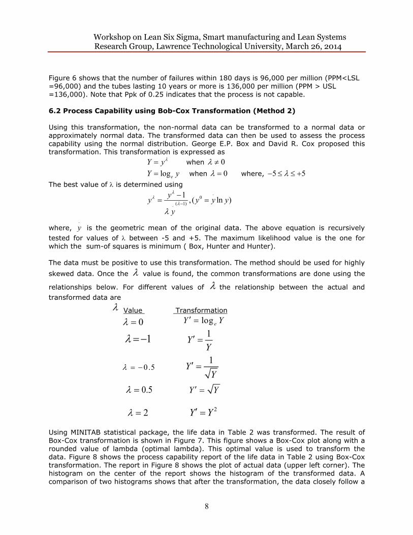
Figure 6 shows that the number of failures within 180 days is 96,000 per million (PPM<LSL =96,000) and the tubes lasting 10 years or more is 136,000 per million (PPM > USL =136,000). Note that Ppk of 0.25 indicates that the process is not capable. 6.2 Process Capability using Bob-Cox Transformation (Method 2) Using this transformation, the non-normal data can be transformed to a normal data or approximately normal data. The transformed data can then be used to assess the process capability using the normal distribution. George E.P. Box and David R. Cox proposed this transformation. This transformation is expressed as Y y when 0

logeY y when 0 where, 5 5 The best value of is determined using

.

0( 1).

1, ( ln )

yy y y y

y

where, .

y is the geometric mean of the original data. The above equation is recursively tested for values of between -5 and +5. The maximum likelihood value is the one for which the sum-of squares is minimum ( Box, Hunter and Hunter). The data must be positive to use this transformation. The method should be used for highly skewed data. Once the value is found, the common transformations are done using the

relationships below. For different values of the relationship between the actual and transformed data are

Value Transformation

0 log eY Y

1 1

YY

0 .5 1

YY

0.5 Y Y

2 2Y Y

Using MINITAB statistical package, the life data in Table 2 was transformed. The result of Box-Cox transformation is shown in Figure 7. This figure shows a Box-Cox plot along with a rounded value of lambda (optimal lambda). This optimal value is used to transform the data. Figure 8 shows the process capability report of the life data in Table 2 using Box-Cox transformation. The report in Figure 8 shows the plot of actual data (upper left corner). The histogram on the center of the report shows the histogram of the transformed data. A comparison of two histograms shows that after the transformation, the data closely follow a


9

normal distribution therefore; a normal distribution can be applied to determine the process capability. The statistics and capability indexes are calculated and shown in Figure 8. From the report, PPM < USL is 96,000 and PPM > LSL is 136,00. These values are the same as found by the process capability using the Exponential distribution in Figure 6. The upper left box in Figure 8 provides the statistics of the process data before and after the transformation.

Lambda

StD

ev

3210-1

35000

30000

25000

20000

15000

10000

5000

0

Lower CL Upper CL

Limit

Lambda

0.19

(using 95.0% confidence)

Estimate 0.19

Lower CL 0.06Upper CL 0.34

Rounded Value

Box-Cox Plot of Life of Monochrome Picture Tube

Figure 7: Box-Cox Plot with Estimated Optimal Lambda Value

6.005.254.503.753.002.251.50

LSL* USL*transformed dataProcess Data

Sample N 125StDev (Within) 1686.51StDev (O v erall) 1616.22

A fter TransformationLSL* 2.70737Target*

LSL

*USL* 4.82199Sample Mean* 3.8235StDev (Within)* 0.94451StDev (O v erall)* 0.850677

180Target *USL 3650Sample Mean 1678.38

Potential (Within) C apability

C C pk 0.37

O v erall C apabilityPp 0.41PPL 0.44PPU 0.39Ppk

C p

0.39C pm *

0.37C PL 0.39C PU 0.35C pk 0.35

O bserv ed PerformancePPM < LSL 96000.00PPM > USL 136000.00PPM Total 232000.00

Exp. Within PerformancePPM < LSL* 118660.84PPM > USL* 145222.72PPM Total 263883.56

Exp. O v erall PerformancePPM < LSL* 94750.80PPM > USL* 120247.12PPM Total 214997.92

WithinO v erall

Process Capability of Life of Monochrome Picture TubeUsing Box-Cox Transformation With Lambda = 0.19

Figure 8: Process Capability Report of Life Data using Bob-Cox Transformation


10

6.3 Process Capability using Johnson’s Transformation (Method 3) Johnson’s transformation is another method to transform a non-normal data to a normal data. Normal L. Johnson proposed this transformation. The method comprises of a family of curves including (1) SB: Bounded, (2) SL: Log Normal and (3) SU: Unbounded. A detailed description on the use of Johnson curves can be found in the paper by Nicholas R. Farnum (1996-97). The life data in Table 2 was transformed using Johnson’s method. Figure 9 shows the probability plot, Anderson-Darling statistics and p-value for the original and transformed data. Figure 10 shows the histogram of the transformed data. The plot of the original data is shown in Figure 4. Note how the distribution in Figure 4 is transformed to normality.

Per

cent

50000-5000

99.9

99

90

50

10

1

0.1

N 125AD 5.506P-Value <0.005

Per

cent

420-2

99.9

99

90

50

10

1

0.1

N 125AD 0.199P-Value 0.883

Z Value

P-V

alue

for

AD

tes

t

1.21.00.80.60.40.2

0.8

0.6

0.4

0.2

0.0

0.94

Ref P

P-Value for Best Fit: 0.882901Z for Best F it: 0.94Best Transformation Type: SBTransformation function equals1.35296 + 0.700728 * Log( ( X + 21.3515 ) / ( 8688.18 - X ) )

P r oba bility P lo t fo r O r ig ina l Da ta

P r o ba bility P lo t fo r T r a nsfor m e d Da ta

Se le ct a T r a nsfor m a tion

(P -Value = 0.005 means <= 0.005)

Johnson Transformation for Life of Monochrome Picture Tube

Figure 9: Probability Plots for Actual, Transformed Data and Transformation Function

Life

Freq

uenc

y

3210-1-2-3

30

25

20

15

10

5

0

Histogram of Tranransformed Data

Figure 10: Histogram of Transformed Data (using Johnson Transformation)


11

Since the data is now transformed to a normal distribution, we can perform a process capability analysis of the transformed data using the normal distribution.

3210-1-2-3

LSL USLProcess Data

Sample N 125StDev(Within) 1.09426StDev(Overall) 0.995668

LSL -1.25034Target *USL 1.13601Sample Mean 0.0205853

Potential (Within) Capability

CCpk 0.36

Overall Capability

Pp 0.40PPL 0.43PPU 0.37Ppk

Cp

0.37Cpm *

0.36CPL 0.39CPU 0.34Cpk 0.34

Observed PerformancePPM < LSL 96000.00PPM > USL 136000.00PPM Total 232000.00

Exp. Within PerformancePPM < LSL 122729.89PPM > USL 154020.27PPM Total 276750.16

Exp. Overall PerformancePPM < LSL 100897.34PPM > USL 131297.65PPM Total 232194.98

WithinOverall

Process Capability using Johnson Transformation

Figure 11: Process Capability Report of Life Data using Johnson Transformation

The process capability report using Johnson transformation is shown in Figure 11. Compare this report to the capability report using Box-Cox transformation in Figure 8 and the report using the distribution fit in Figure 6. They are very similar. The PPM < LSL and PPM>USL are 96,000 and 136,000 are the same for all three methods. 7.0 Summary This paper examined the process capability evaluation techniques for non-normal data, and provided cases and analysis techniques for such data. The non-normal process capabilities were evaluated by (1) identifying and using the correct distribution, (2) using the distribution fit approach; where, an appropriate distribution was fitted to describe the data and the fitted distribution was used to determine the process capability, (3) transforming the non-normal data to a normal data using the Box-Cox Transformation then using the Box-Cox transformation method to assess the process capability, and (4) transforming the non-normal data using Johnson Transformation, and assessing the process capability using Johnson’s transformation. The results of the methods (2) through (4) showed that the process capability using all these three methods is identical. The paper also outlined different methods of dealing with non-normal data and the importance of using the correct methods in assessing the process capability for non-normal data. Determining the correct process capability in Six Sigma is critical to assessing the current and improved performance. During a Six Sigma project, the process capability is evaluated twice; first


12

during the measure phase to show the impact of the problem and again after the improvement phase to show how the process has improved. Correct evaluation of process capability is critical to the success of a Six Sigma program. This paper addressed the importance and correct evaluation of process capability. References:

1. AIAG, “Statistical Process Control,” Reference Manual, 2nd Edition, July 2005. 2. Douglas C. Montgomery, Introduction to Statistical Process Control, 4th Edition, John

Willy and Sons, 2004. 3. John A. Clements, “Process Capability Calculations for Non-Normal distributions,”

Quality Progress, September 1989. 4. MINITAB statistical Software, Release 16. 5. Nicholas R. Farnum, Modern Statistical Quality Control and Improvement, Duxbury

Press, CA, 1994. 6. Nicholas R. Farnum, “Using Johnson Curves to Describe Non-Normal Data,” Quality

Engineering, 9(2), 1996-97. 7. Sahay Amar, Six Sigma Quality: Concepts & Cases-Volume I, Statistical Tools and

Applications in Six Sigma DMAIC Process using MINITAB, 2013 (ISBN - 13:978-0-9850446-3-3) AMT Publishing, Digital Solutions, Salt Lake City, UTAH.

If you are interested in Process Capability Analysis, Measurement Systems Analysis (Gage R&R), Quality Tools (Basic and New Tools) and Six Sigma Tools with MINITAB applications and cases, check out the following tittle.

Sahay Amar, Six Sigma Quality: Concepts & Cases-Volume I, Statistical Tools and Applications in Six Sigma DMAIC Process using MINITAB, 2013 (ISBN - 13:978-0-9850446-3-3) AMT Publishing, Digital Solutions, Salt Lake City, UTAH.

You can get the details on the following website: www.realleansixsigmaquality.com You can obtain a copy of the entire book, the chapter(s) you are interested in, or the chapters in power point slide format.

Six Sigma Process Capability Analysis When the …...Six Sigma Process Capability Analysis When the...

Documents

Transcript of Six Sigma Process Capability Analysis When the …...Six Sigma Process Capability Analysis When the...