SCOTTISH INSTITUTE FOR RESEARCH IN ECONOMICS

SIRE DISCUSSION PAPER SIRE-DP-2015-36

Meeting Technologies and Optimal Trading Mechanisms in

Competitive Search Markets

 Benjamin Lester Ludo Visschers Ronald Wolthoff  

UNIVERSITY OF EDINBURGH

  

www.sire.ac.uk

Meeting Technologies and Optimal TradingMechanisms in Competitive Search Markets∗

Benjamin Lester†

Federal Reserve Bank of PhiladelphiaLudo Visschers‡

University of Edinburgh& Universidad Carlos III, Madrid

Ronald WolthoffUniversity of Toronto

August 2, 2014

Abstract

In a market in which sellers compete by posting mechanisms, we study how the properties ofthe meeting technology affect the mechanism that sellers select. In general, sellers have incen-tive to use mechanisms that are socially efficient. In our environment, sellers achieve this byposting an auction with a reserve price equal to their own valuation, along with a transfer thatis paid by (or to) all buyers with whom the seller meets. However, we define a novel conditionon meeting technologies, which we call “invariance,” and show that the transfer is equal tozero if and only if the meeting technology satisfies this condition.

JEL classification: C78, D44, D83.Keywords: search frictions, matching function, meeting technology, competing mechanisms.

∗We would like to thank Philipp Kircher, Guido Menzio and Gabor Virag for helpful comments. All errors are ourown.†The views expressed here are those of the authors and do not necessarily reflect the views of the Fed-

eral Reserve Bank of Philadelphia or the Federal Reserve System. This paper is available free of charge atwww.philadelphiafed.org/research-and-data/publications/working-papers/.‡Ludo Visschers gratefully acknowledges financial support from the Juan de la Cierva Grant; project grant

ECO2010-20614 (Direccion general de investigacion cientıfica y tecnica), and the Bank of Spain’s Programa de In-vestigacion de Excelencia.

1

1 Introduction

What trading mechanism should a seller use to sell a good? This is a classic question in economicsand the answer, of course, depends on the details of the environment. We study this question inan environment with three key ingredients. First, there are a large number of sellers and a largenumber of buyers, each seller has one indivisible good, and sellers compete for buyers by postingthe trading mechanism they will use to sell their good. Then, buyers observe the mechanisms thathave been posted and choose the one that promises the maximal expected payoff, but the processby which buyers and sellers meet is frictional. In particular, when a buyer chooses to visit a seller,there may be uncertainty about whether he is actually able to meet with that seller, as well as thenumber of other buyers who also meet with that seller; we call the function that governs this processthe “meeting technology.” Finally, after buyers meet with a seller, they learn their idiosyncraticprivate valuation for the seller’s good.

In this environment, we provide a complete characterization of the mechanism that sellerschoose in equilibrium. More specifically, we show that sellers can do no better than a second-priceauction with a reserve price equal to their own valuation and a fee (or subsidy) that is paid by (orto) each buyer that participates. We characterize this fee in closed form. Then, in the same spiritas Eeckhout & Kircher (2010), we study how this optimal mechanism depends on the propertiesof the meeting technology.

Our results suggest that conclusions drawn in the existing literature may depend quite heavilyon the specific functional form that has typically been chosen for the meeting technology. In par-ticular, previous studies of this basic environment (e.g., Peters (1997), Peters & Severinov (1997),Albrecht et al. (2012, 2013, 2014) and Kim & Kircher (2013)) have shared three features in com-mon. First, the equilibrium in these papers is constrained efficient, in the sense that the solution tothe planner’s problem is implemented. Second, the trading mechanism that implements the con-strained efficient allocation only requires transfers between the two agents that ultimately trade, sothat agents who do not trade are not required to pay a fee nor are they offered a subsidy. Last, allof the papers cited above assume the same functional form for the meeting technology—what isoften called the “urn-ball” meeting technology.

Taken together, the first two properties are somewhat surprising. After all, constrained effi-ciency places strict requirements on two distinct margins. First, from an ex ante point of view,it requires the proper allocation of buyers to sellers. Second, from an ex post point of view, itrequires the proper allocation of the good once buyers arrive at a seller and learn their valuations.In order to implement an equilibrium that satisfies these two requirements, the payoffs receivedby buyers and sellers must inherit certain properties: to satisfy the first requirement, each buyer

2

must receive an expected payoff exactly equal to his marginal contribution to the match surplus;1

however, to satisfy the second requirement, payoffs must ensure that buyers truthfully report theirvaluation and that the good is allocated to the agent with the highest valuation. In principle, thereis no reason to think that the payoffs satisfying the former requirement should coincide with thepayoffs satisfying the latter.

We show that, in fact, these payoffs coincide—or, equivalently, that the meeting fee in the opti-mal mechanism is equal to zero—if, and only if, the meeting technology satisfies a novel conditionthat we call invariance. Loosely speaking, a meeting technology is invariant if the decision by onebuyer to visit the mechanism a seller has posted does not interfere with the process by which thatseller meets with other buyers. When invariance is violated, one buyer’s search decision exerts anexternality on the meeting prospects of the seller with other buyers, and this externality needs tobe taxed (or subsidized).

The urn-ball process is one example of a meeting technology that satisfies invariance, whichexplains why the optimal mechanism in previous studies was so simple and why additional (rarelyobserved) side payments were not necessary. However, the urn-ball meeting technology also sat-isfies several other properties that previous studies have conjectured are important for determiningthe optimal trading mechanism. We close our analysis by comparing one of these properties—what Eeckhout & Kircher (2010) call “non-rivalry”—with our invariance property. We show thatnon-rivalry is a necessary (but not sufficient) condition for invariance.

2 Environment

Agents and Preferences. The economy is populated by a measure µB > 0 of buyers and ameasure µS > 0 of sellers, with Λ = µB

µS.2 Each seller possesses one, indivisible good and each

buyer has unit demand for this good. All agents are risk neutral.Sellers value their own good at y, which is common knowledge, while buyers have to visit

a seller in order to learn their valuation. In particular, after a buyer meets a seller, he learns hisprivate valuation x for that seller’s good, which is drawn from a twice continuously-differentiabledistribution F (x) with support [x, x] ⊂ R+. An individual buyer’s valuations are i.i.d. acrosssellers, as are the valuations of each buyer at an individual seller. We assume that y ∈ [x, x).3

1For detailed discussions of the relationship between the division of surplus and efficiency in search environments,see, e.g., Mortensen (1982), Hosios (1990) and Moen (1997).

2Though we focus our attention on an environment with an exogenous measure of sellers, our results do not changeif we endogenize the measure of sellers through a free entry condition. We prove this formally in the Appendix.

3Since we do not impose much structure on F (x), this is a fairly weak assumption, as the probability that a buyer’svaluation x is smaller than y can be driven to zero without any loss of generality.

3

Mechanisms. In order to attract buyers, each seller posts and commits to a direct mechanism.A mechanism specifies an extensive form game that determines for each buyer i a probability oftrade and an expected payment as a function of: (i) the total number n of buyers to meet with theseller; (ii) the valuation xi that buyer i reports; and (iii) the valuations x−i reported by the n − 1

other buyers. Formally, a mechanism is summarized by a probability of trade φ(xi, x−i, n) and atransfer τ(xi, x−i, n) for all n ∈ N1 ≡ {1, 2, 3, . . .} and i ∈ {1, 2, ...n}.

Meeting Technology. After observing all posted mechanisms, each buyer chooses the mecha-nism at which he will attempt to trade. However, the meeting process between buyers and sellersis frictional, so that some buyers may not meet a seller and some sellers may not meet with anybuyers.4 As is often done in the literature, we restrict attention to meeting technologies that ex-hibit constant returns to scale. More specifically, suppose a measure σ of sellers post the samemechanism and a measure β of buyers choose this mechanism. Then, letting λ = β/σ denote themarket tightness or queue length at that mechanism, a seller meets exactly n ∈ N0 ≡ {0, 1, 2, . . .}buyers with probability Pn (λ).5 We assume that Pn (λ) is twice continuously-differentiable. Sincethe number of meetings cannot exceed the number of buyers who attempt to trade at a particularmechanism, the probability distribution must satisfy

∑∞n=0 nPn (λ) ≤ λ.

We denote the probability for a buyer to meet a seller with exactly n−1 other buyers byQn (λ).This probability is related to Pn (λ) through the consistency requirement

nPn (λ) = λQn (λ) , (1)

for all n ∈ N1. Intuitively, given market tightness λ = β/σ at some mechanism, the measure ofbuyers at those sellers who end up with precisely n buyers, σnPn(λ), must equal the measure ofbuyers who face n−1 buyers at their seller, βQn(λ). Finally, we defineQ0 (λ) = 1−

∑∞n=1 Qn (λ)

as the probability that the buyer fails to meet with a seller.

Probability-Generating Function. It will prove useful to define the function

m (z;λ) ≡ E [zn|λ] =∞∑n=0

Pn (λ) zn (2)

4Note that our language follows that of Eeckhout & Kircher (2010), who make the distinction between meetingsand matches. All buyers who participate in a seller’s trading mechanism are said to “meet” with the seller, whereasthe buyer who acquires the seller’s single, indivisible good is said to “match” with the seller.

5We follow most of the literature by assuming that the process through which buyers and sellers meet is exogenous.Only a small number of papers derive the meeting technology as the endogenous outcome of agents’ optimal decisions.See Lester et al. (2013) for an example.

4

for z ∈ [0, 1] with, by convention, m (0;λ) = P0 (λ). This function is the probability-generatingfunction of n and provides an alternative representation of Pn (λ), as Pn (λ) = 1

n!∂n

∂znm (0;λ) . As

we will see below, introducing the notation and tools of probability-generating functions allowsus to derive a number of results that would be more difficult to obtain using standard techniquesfrom the directed search literature. In particular, it will be helpful to note that, setting z = F (x),m (z;λ) can be interpreted as the probability that the maximum valuation at a seller with a queuelength λ is no greater than x.6

Let mz and mλ denote the partial derivative of m (z;λ) with respect to the first and secondargument, respectively. Given the properties of a probability-generating function, the expectednumber of meetings per unit mass of sellers can then be expressed as

∞∑n=0

nPn (λ) = mz (1;λ) . (3)

Note that mz (·) > 0, with m (·) ranging from m (0;λ) = P0 (λ) to m (1;λ) = 1. In addition, weimpose that mλ (z;λ) < 0 and mλλ (z;λ) ≡ ∂2

∂λ2m (z;λ) > 0 for all z ∈ [0, 1) and λ ∈ (0,∞).

Again letting z = F (x), these assumptions imply that a marginal increase in the queue lengthalways reduces the probability that the maximum valuation at a seller is below x = F−1(z), butthat the effect is smaller when the queue length is longer.7

3 The Planner’s Problem and Market Equilibrium

In this section, we first characterize the solution to the planner’s problem, and then characterizethe decentralized market equilibrium.

3.1 The Planner’s Problem

Consider the problem of a benevolent social planner whose objective is to maximize net socialsurplus, subject to the frictions of the physical environment (e.g., the meeting frictions). Theplanner’s decision rule can be broken down into two components. First, the planner has to assignqueue lengths to each seller, subject to the constraint that the sum of these queue lengths acrossall sellers cannot exceed the total measure of available buyers. Second, the planner has to specifya trading rule for agents to follow after buyers arrive at sellers. We solve these stages in reverseorder. As the derivation is standard for each component, we keep the exposition brief.

6If no buyers arrive, the maximum valuation is, by convention, −∞.7Monotonicity of m (·) in λ is implied if a change in λ causes a first-order stochastic dominance shift in Pn (λ).

Convexity is also common in the literature; see, e.g., Eeckhout & Kircher (2010) for a similar assumption.

5

Trading Rule. Consider a seller who is visited by n buyers. Clearly, the surplus at this seller ismaximized by instructing the seller to trade with the buyer who has the highest valuation x if thisvaluation exceeds y, and keep the good himself otherwise. Therefore, the expected net surplus at aseller with queue length λ is

S (λ) =∞∑n=0

Pn (λ)

∫ x

y

(x− y) dF n (x) = x− y −∫ x

y

m (F (x) ;λ) dx. (4)

Allocation of Buyers. Now consider the allocation of buyers to sellers. At this stage, the objec-tive of the planner is to choose queue lengths at each seller, i.e., λj for j ∈ [0, µS], to maximize∫ µS

0S (λj) dj subject to the constraint that

∫ µS0

λjdj = µB. As S ′′ (λ) = −mλλ (F (x) ;λ) < 0,it follows immediately that the planner maximizes total surplus by assigning equal queue lengthsacross all sellers, so that λj = Λ = µB

µSfor all j and total surplus equals

∫ µS0

S (Λ) dj = µSS (Λ) .

The following proposition summarizes.

Proposition 1. A unique solution to the planner’s problem exists. In this solution, each seller is

assigned a queue length Λ. After buyers arrive and learn their valuation, the planner assigns the

good to the agent with the highest valuation.

3.2 Market Equilibrium

To characterize the relevant properties of the mechanism that sellers select in equilibrium, weproceed in two steps. First, we restrict attention to second-price auctions with a reserve price r anda meeting fee t that is paid by (or to) each buyer before learning his type. Within this restricted setof mechanisms, we define an equilibrium and characterize the profit-maximizing values of r andt. Then, we establish that sellers can do no better than this second-price auction, even with accessto the set of all direct mechanisms. More specifically, we show that any direct mechanism chosenby a seller in equilibrium will be payoff-equivalent to the second-price auction with r and t chosenoptimally.

Equilibrium with Second-Price Auctions and Meeting Fees. As a first step, we calculate theexpected revenue of a seller who sets r and t and attracts a queue length λ, along with the expectedpayoff of each buyer that visits this seller.

Lemma 1. A seller who posts a second-price auction with reserve price r and meeting fee t who

6

attracts a queue λ obtains an expected payoff equal to

R (r, t, λ) = x− (r − y)m (F (r) ;λ)−∫ x

r

m (F (x) ;λ) dx

−∫ x

r

(1− F (x))mz (F (x) ;λ) dx+ tmz (1;λ) .

The expected payoff for each buyer in the seller’s queue equals

U (r, t, λ) =1

λ

∫ x

r

(1− F (x))mz (F (x) ;λ) dx− t

λmz (1;λ) . (5)

A seller’s objective is to maximize revenue, taking into account that his choice of r and t

affects the queue λ that he attracts. In particular, optimal search behavior implies that buyers mustbe indifferent between all sellers who receive a strictly positive queue. Formally, let U denote thehighest level of utility that buyers can obtain in this market, or what is often called the “marketutility.” Then, the equilibrium relationship between r, t, and λ is determined by U (r, t, λ) = U .

Hence, an equilibrium in this environment is formally a distributionG (r, t, λ) of reserve prices,meeting fees, and queue lengths across sellers, and a market utility U , such that (i) given U ,each triple (r, t, λ) in the support of G maximizes revenue R (r, t, λ) subject to the constraintU (r, t, λ) = U ; and (ii) aggregating queue lengths across all sellers yields the total measure ofbuyers, µB. However, one can prove that there exists a unique equilibrium in which all sellers postthe same reserve price r∗ and meeting fee t∗, and attract the same queue λ∗ = Λ. Moreover, itturns out that the optimal reserve price is equal to the sellers’ valuation (r∗ = y), so that the goodis allocated to the agent (one of the buyers or the seller) with the highest valuation. Hence, thedecentralized equilibrium is constrained efficient, i.e., it creates the same amount of surplus as theplanner’s solution. The following proposition summarizes and derives t∗ in closed form.

Proposition 2. A unique equilibrium exists and it is constrained efficient. In equilibrium, the

reservation price equals r∗ = y, the meeting fee equals

t∗ =Λ

mz (1; Λ)

∫ x

y

[1

Λ(1− F (x))mz (F (x) ; Λ) +mλ (F (x) ; Λ)

]dx, (6)

and the queue length equals λ∗ = Λ at all sellers, with buyers receiving market utility U =

U(r∗, t∗,Λ).

Intuitively, the first term in brackets in (6) is the buyer’s private expected payoff from partici-pating in an auction with reserve price r = y when the queue length is Λ, which is evident from(5). The second term in brackets is the (negative value of) this buyer’s marginal contribution to

7

the social surplus generated by the auction, which is evident from (4). Hence, t∗ is simply thedifference between the two, adjusted to account for the fact that not every buyer actually meets theseller and pays this fee.

Equilibrium with General Mechanisms. Proposition 2 describes the equilibrium outcome whensellers have access to a restricted set of mechanisms and shows that the equilibrium coincides withthe solution to the planner’s problem. In Proposition 3 below, we establish that sellers would notbenefit from having access to a larger set of mechanisms; both the expected payoffs and the alloca-tions will be identical in any other equilibrium. The reasoning is simple: since buyers’ equilibriumpayoffs are equal to the market utility U , an individual seller is the residual claimant on any ad-ditional surplus he creates. Hence, he has incentive to select an efficient mechanism in order tomaximize this surplus. The mechanism that we consider—a second-price auction with a reserveprice r and a meeting fee t—is sufficiently flexible that it allows the seller to maximize the “sizeof the pie” without placing restrictions on how the pie is divided. Therefore, access to additionalmechanisms is largely irrelevant.8

Proposition 3. A mechanism {φ(xi, x−i, n), τ(xi, x−i, n)} is an equilibrium if, and only if, it is

payoff-equivalent to the equilibrium characterized in Proposition 2.

4 Meeting Technologies and the Optimal Mechanism

In the previous section, we characterized the equilibrium mechanism that arises in a fairly generalenvironment. An important feature of the optimal mechanism is a meeting fee, t∗, that allowssellers to manipulate expected revenue without distorting the efficient allocation. Somewhat sur-prisingly, this meeting fee does not play a role in the optimal mechanism that has been identified inthe previous literature. Rather, these papers find that the optimal mechanism is simply an auctionwith reserve price r∗ = y.

We now reconcile our results with the existing literature by showing that previous studies hadfocused on a special class of meeting functions. In particular, we introduce a novel property ofmeeting technologies that we call invariance and show that this property is necessary and suffi-cient for t∗ = 0. We use several examples to illustrate the relationship between invariance and thenecessity of meeting fees. We then conclude by reviewing another property of meeting technolo-gies that has been identified in the literature and discuss its relationship to invariance.

8One may also wonder whether there exists an alternative equilibrium in which sellers use a mechanism that onlyrequires the buyer who trades to pay a transfer, and leaves all other buyers with a payoff of zero. In the Appendix, weshow that the answer is “no.”

8

4.1 Invariance

We now introduce a property of meeting technologies that we call “invariance,” which requiresthat the probability of a seller meeting with n members of any subset of buyers in the queue isunaffected by the presence (or lack thereof) of buyers in the queue who are outside of this subset,for all n ∈ N0. To formalize this concept, suppose that each buyer is assigned a certain label withprobability γ ∈ [0, 1], independent of the realizations of this label for other buyers. Then, theprobability that a seller meets exactly n buyers with this label equals9

Pn (λ, γ) ≡∞∑N=n

PN (λ)

(N

n

)γn (1− γ)N−n .

Definition 1. A meeting technology is invariant if, and only if, Pn (λ, γ) = Pn (γλ) for all γ ∈(0, 1), λ ∈ (0,∞), and all n ∈ N0.

To understand the intuition, consider a sub-market in which the ratio of buyers to sellers is λ,and suppose that a fraction γ of buyers are red and the remainder are green.10 Invariance, then, saysthat the ratio of red buyers to sellers must be a sufficient statistic for the distribution that governsthe number of red buyers who arrive at a seller. In particular, changing the measure of green buyersshould not change the probability that n red buyers arrive at a seller, for any n ∈ N0.

In other words, a marginal buyer choosing to visit the mechanism a seller has posted doesnot interfere with the process by which that seller meets with other buyers. When the invariancecondition is violated, the seller either wants to tax or subsidize buyers for choosing his mechanism,depending on whether they exert a negative or positive externality on his prospects for meetingother buyers, respectively. The proposition below formalizes this argument: we establish thatmeeting fees are set to zero in equilibrium if, and only if, the meeting technology is invariant, andwe derive a simple condition for verifying invariance for arbitrary technologies.

Proposition 4. Consider a meeting technology Pn (λ). The following statements are equivalent:

1. Meeting fees are not used in equilibrium, i.e., t∗ = 0 for any distribution F (x) with support

[x, x] ⊂ [0,∞), y ∈ [x, x) and Λ ∈ (0,∞);

2. The meeting technology is invariant;

9This transformation, introduced by Renyi (1956), is known as “binomial thinning.” See Harremoes et al. (2010).10Note that labeling buyers “red” and “green” is simply a convenient device to split the queue into subsets. Indeed,

different labels can be arbitrarily assigned to ex ante homogeneous buyers, which will be the case in our analysis, orthey can be assigned to buyers that are ex ante heterogeneous, as we discuss in Section 4.2. For the purpose of defininginvariance, it does not matter. It does, however, slightly change the intuition in some of our explanations below. Inwhat follows, we find it easiest to convey the intuition by treating a buyer’s color as being realized ex ante, but thediscussion could easily be adapted to treat the alternative case as well.

9

3. The meeting technology can be written as

Pn (λ) =(−λ)nM (n) (λ)

n!, (7)

for some function M : [0,∞) → [0, 1] that satisfies m (z;λ) = M (λ (1− z)) and pre-

serves all of our assumptions on Pn (λ) and m (z;λ), with M (n) (·) denoting the nth-order

derivative of M .11

4.2 Discussion

Examples of Meeting Technologies. In order to facilitate a discussion of the invariance condi-tion introduced above, it will be helpful to introduce a few examples of meeting technologies.

1. Urn-Ball. Popular in the directed search literature, this specification arises when a measureβ of buyers randomize evenly across a measure σ of sellers who have posted the same mech-anism.12 As a result, the number of buyers that visit a particular seller is determined by aPoisson distribution with mean equal to λ = β/σ. That is, Pn (λ) = e−λ λ

n

n!.

2. Geometric. The geometric meeting technology specifies that Pn(λ) = λn

(1+λ)n+1 . Again,letting λ = β/σ, this meeting technology can be interpreted as the outcome of a process inwhich a mass β of buyers and a mass σ of sellers are randomly positioned on a circle, andbuyers walk to the nearest seller to their right.

3. Bilateral. This specification, often used in the literature that uses search-theoretic modelsto study monetary theory, has the following interpretation.13 Suppose there is a mass β andσ of buyers and sellers, respectively, and all agents are randomly matched in pairs. Then,given λ = β/σ, the probability distribution over the number of buyers that a seller meets is:P0 (λ) = 1

1+λ, P1 (λ) = λ

1+λ, and Pn (λ) = 0 for n ∈ {2, 3, . . .}.

4. Pairwise Urn-Ball. If a measure β of buyers are first grouped in pairs and then allocatedacross a measure σ of sellers according to the urn-ball technology described above then, let-ting λ = β/σ, the meeting technology can be described by Pn (λ) = 0 for n ∈ {1, 3, 5, . . .}and Pn (λ) = e−λ/2 (λ/2)n/2

(n/2)!for n ∈ {0, 2, 4, . . .}.

There are several things to note from these examples. First, the urn-ball technology satisfies theinvariance condition: when all buyers randomize across a group of sellers, the presence of more

11For the sake of completeness, we describe exactly which properties of M are necessary to preserve our assump-tions on Pn and m in the Appendix.

12This specification was first used by Butters (1977) and Hall (1977). See Burdett et al. (2001) for an explicitderivation of the micro-foundations of this meeting technology in a directed search model.

13See, e.g., Kiyotaki & Wright (1993) and Trejos & Wright (1995). This technology has also been used morerecently to study trading dynamics in over-the-counter financial markets; see, e.g., Duffie et al. (2007).

10

green buyers has no effect on the number of red buyers to arrive at a particular seller. Since theexisting literature has focused primarily on the case of urn-ball matching, it should then come as nosurprise that a simple second-price auction with r∗ = y was identified as the optimal mechanism.

Second, since the geometric technology satisfies (7) for M (λ) = 11+λ

, this meeting technologyalso satisfies invariance: since a red buyer meets with the first seller to his right, it is irrelevant(by construction) how many green buyers he passes on his way.14 This confirms that the set ofinvariant meeting technologies is not limited to derivatives of the urn-ball process, but acceptsother reasonable meeting processes as well.

Third, note that the bilateral meeting technology is not invariant: since sellers only meet withone randomly selected buyer under this meeting technology, an increase in the measure of greenbuyers will decrease the probability that a seller meets one red buyer (and increase the probabilityhe meets zero red buyers). Hence, in a competitive environment with this meeting technology,sellers would optimally employ a meeting fee to tax this congestion externality appropriately.

Lastly, note that the pairwise urn-ball technology also violates invariance. Intuitively, whenthe measure of green buyers is insignificant, most red buyers are matched in pairs with other redbuyers and it is highly likely that a seller is visited by an even number of red buyers. As themeasure of green buyers gets large, however, it becomes increasingly likely that red buyers arepaired with green buyers, which implies a greater probability that a seller is visited by an oddnumber of red buyers. Hence, this process is not invariant. However, in contrast to the bilateralmeeting technology, buyers exert a positive externality on one another under the pairwise urn-ballmeeting process, and thus sellers optimally offer a meeting subsidy in equilibrium (i.e., t∗ < 0).

Non-Rivalry. We close our analysis by comparing the invariance condition to another propertyof meeting technologies that has been identified in the literature: what has often been called “non-rivalry.” In addition to distinguishing our results from the existing literature, this comparison alsosheds light on other environments in which the invariance condition is likely to be an importantdeterminant of the optimal mechanism for price (or wage) determination.

In words, Eeckhout & Kircher (2010) describe a (purely) non-rival meeting technology as onein which “the meeting probability for a buyer is not affected by the presence of other buyers in themarket.”15 That is, 1 − Q0 (λ) is independent of λ. Using the definition of Q0 (λ), it is easy toverify that this condition is equivalent to the requirement that there exists a γ ∈ [0, 1], such that∑∞

n=0 nPn (λ) = γλ for all λ.16

14More generally, the family of negative-binomial distributions satisfies equation (7) for M (λ) =(

θθ+λ

)θand

θ ∈ N1. This family of distributions is therefore invariant as well.15For a recent example of a paper that cites the importance of non-rivalry, see Albrecht et al. (2014).16Note that

∑∞n=1Qn (λ) =

1λ

∑∞n=0 nPn (λ).

11

Clearly the urn-ball technology described earlier in the text is non-rival because each buyermeets a seller with probability one. The bilateral meeting technology, however, violates non-rivalry. Since each seller can meet at most one buyer, an increase in the ratio of buyers to sellersimplies that each buyer is more likely to be crowded out. As a result, the probability that eachbuyer meets a seller, 1 − Q0 (λ) = 1−e−λ

λ, is decreasing in λ. Given these observations, a natural

question is how non-rivalry relates to invariance, which we address in the following lemma.17

Lemma 2. Invariance implies non-rivalry, but non-rivalry does not imply invariance.

To understand the first statement in Lemma 2, it is helpful to recall our previous example,where buyers are either red or green. If the meeting technology does not satisfy non-rivalry, thenincreasing the measure of green buyers, while holding constant the measure of sellers and redbuyers, will decrease the probability that each red buyer meets a seller. This implies that increasingthe measure of green buyers will decrease the probability that a seller meets with n ≥ 1 redbuyers, which violates the invariance condition. The second statement in the lemma follows fromconsidering the pairwise urn-ball technology. This technology is non-rival since each buyer meetsa seller with probability one, regardless of the ratio of buyers to sellers. However, as we explainedabove, it is not invariant.

Intuitively, non-rivalry is a statement about whether a buyer’s decision to visit a sub-market (ormechanism) affects the probability that another buyer will meet a seller in that sub-market, whileinvariance is a statement about whether an individual buyer’s decision to visit a sub-market affectsthe distribution of buyers at each seller in that sub-market. Given this distinction, we concludethat whether or not a meeting technology is invariant is likely to be a crucial determinant of theoptimal trading mechanism in any environment where the payoff of a seller (or firm) depends onthe distribution of buyers (or workers) that arrive. In this paper, we provided perhaps the simplestenvironment where the distribution of buyers is relevant: when buyers draw independent valuationsafter choosing a seller, a key object of interest for the seller is the maximum valuation among allbuyers—an order statistic—which clearly depends on whether there are two or three or four buyers.

However, by this logic, invariance is also likely to be an important property of the meetingtechnology in models of directed search in which buyers can attempt to meet multiple sellers, asin Albrecht et al. (2006) and Galenianos & Kircher (2009). In these models, ex post heterogeneityarises because some buyers have received two price quotes and others have received only one; aseller’s trading probability is thus 1 − P0 (λ, γ), where γ is the fraction of buyers that don’t tradewith a different seller. As such, our results suggest that meeting fees will likely be needed to price

17In the Appendix, we compare invariance to a third property of meeting technologies that the urn-ball technologyalso satisfies, which we call “independence.” Put succinctly, this property requires that the arrival of a buyer at aparticular seller does not change the distribution of other buyers at that seller. We show that independence is neithersufficient nor neccessary for invariance.

12

this externality if the meeting technology is not invariant.18

Importantly, the role of the invariance condition in determining the optimal trading mechanismis not limited to environments with ex post heterogeneity, but is also likely to be important inenvironments with ex ante heterogeneity as well. For example, in a directed search model with exante heterogeneous buyers, if invariance is violated—e.g., if one buyer’s search decision affects thedistribution of other buyers that the seller meets—then our results suggest that standard methodsof price determination may need to be supplemented with fees or subsidies.19 We leave a detailedinvestigation of the role of invariance in models with ex ante heterogeneity for future research.

5 Conclusion

We consider an environment in which sellers compete by posting mechanisms and buyers directtheir search toward the mechanism offering the maximal expected payoff. We characterize thetrading mechanism that sellers choose in equilibrium, given a fairly general class of meeting tech-nologies. We show that, in general, sellers can do no better than posting an auction with no reserveprice, but with a meeting fee (or subsidy) that is paid by (or to) all buyers who participate in theauction. Then, we completely characterize a subset of meeting technologies for which the meet-ing fee is set to zero, and show that the meeting technology that previous studies have used wascontained in this subset. We call the meeting technologies in this subset invariant.

Appendix

Proofs

Proof of Proposition 1. The proof of this result is provided in the main text.

18This is consistent with the results in this literature that wage posting (without meeting fees) decentralizes theplanner’s solution when the meeting technology is urn-ball (Kircher, 2009), but not when firms are constrained in thenumber of applications that they can process (Galenianos & Kircher, 2009; Wolthoff, 2012).

19Indeed, with ex ante heterogeneity, the meeting technology affects both the optimal mechanism and whetherdifferent types of buyers pool or separate in equilibrium: an urn-ball technology leads to perfect pooling, while abilateral technology leads to perfect separation. Peters & Severinov (1997), Virag (2010), Albrecht et al. (2012,2014) and Peters (2013) study the urn-ball case, while Eeckhout & Kircher (2010) analyze both urn-ball and bilateralmeeting technologies. Shi (2001) derives related results in a labor market setting with bilateral meetings, while Shimer(2005) and Peters (2010) study a similar problem with the urn-ball meeting technology. Given our results, a naturalconjecture is that the pooling equilibrium without meeting fees extends to all invariant meeting technologies, whilemeeting technologies with congestion externalities give rise to an equilibrium with meeting fees and at least someseparation of types.

13

Proof of Lemma 1. From the description of the auction in the main text, it follows immediatelythat a buyer’s expected payoff equals

U (r, t, λ) =∞∑n=1

Qn (λ)

[∫ x

r

∫ x

x

(x−max {x, r}) dF n−1 (x) dF (x)− t].

The inner integral simplifies to∫ xrF n−1 (x) dx after integration by parts. Changing the order of

integration and substituting equations (1) and (2) then yields equation (5).To calculate the payoff of a seller, consider the expected valuation V (r, λ) of the agent that

holds the good at the end of the period, given a queue length λ and reserve price r. As the maximumvaluation among n buyers is distributed according to F n (x), V (r, λ) equals

V (r, λ) = P0 (λ) y +∞∑n=1

Pn (λ)

[F n (r) y +

∫ x

r

xdF n (x)

]= x− (r − y)m (F (r) ;λ)−

∫ x

r

m (F (x) ;λ) dx,

where the second line follows after integration by parts and substitution of (2). As the payoff of aseller must satisfy R (r, t, λ) = V (r, λ)− λU (r, t, λ), the desired expression follows.

Proof of Proposition 2. The Lagrangian of the seller’s maximization problem equals

L (r, t, λ, ζ) = R (r, t, λ) + ζ(U (r, t, λ)− U

),

where ζ denotes the multiplier on the market utility constraint. The first-order condition withrespect to t equals (

1− ζ∗

λ∗

)mz (1;λ∗) = 0.

As mz (1;λ) > 0, this implies that ζ∗ = λ∗ in any equilibrium. Substituting this into the first-order condition with respect to r gives (y − r∗)mz (F (r∗) ;λ∗)F ′ (r∗) = 0. Hence, r∗ = y inany equilibrium. In combination with these results, the first-order condition with respect to λ

subsequently implies that the optimal meeting fee must satisfy

t∗ =λ∗

mz (1;λ∗)

∫ x

y

[1

λ∗(1− F (x))mz (F (x) ;λ∗) +mλ (F (x) ;λ∗)

]dx.

14

In combination with the first-order condition with respect to ζ , this implies that the optimal queuelength λ∗ is determined by

−∫ x

y

mλ (F (x) ;λ∗) dx = U. (8)

Since m (z;λ) is convex in λ, a unique solution exists for any U small enough. In equilibrium, themarket utility has to be such that λ∗ = Λ, or otherwise the market clearing constraint

∫ µS0

λ∗dj =

µB is violated. It immediately follows that U = −∫ xymλ (F (x) ; Λ) dx and that the equilibrium is

efficient.

Proof of Proposition 3. This proof closely resembles the corresponding one in Lester et al.(2013) and suppresses the arguments of φ and τ to keep notation concise. Suppose there existsan equilibrium in which one or more sellers post a particular mechanism {φ0, τ0} and attract aqueue length λ0, which yields them a payoff R (φ0, τ0, λ0), yields buyers a market utility U =

U (φ0, τ0, λ0), and creates a surplus S (φ0, λ0) = R (φ0, τ0, λ0)+λ0U (φ0, τ0, λ0)−y.20 A deviantseller who posts a mechanism {φ, τ} and attracts a queue λ, determined by the market utilitycondition U (φ, τ, λ) = U , obtains a payoff

R (φ, τ, λ) = S (φ, λ)− λU + y.

This payoff is maximized when the deviant chooses trading probabilities φ which correspond withthe planner’s solution φ∗, and τ such that

∂

∂λS (φ∗, λ) ≡ d

dλS (λ) = U. (9)

Note that {φ0, τ0} can be part of an equilibrium if, and only if, it is a solution to the deviant’smaximization problem, i.e., φ0 = φ∗ and λ0 solves (9). Strict concavity of S (λ) implies that aunique solution exists to (9) for each level of market utility. Hence, all sellers must attract the samequeue length and this queue length must equal λ = Λ, as any other value is inconsistent with theaggregate buyer-seller ratio. It is easy to verify that d

dλS (λ)

∣∣λ=Λ

= U (r∗, t∗,Λ), which impliesthat {φ0, τ0} is an equilibrium strategy if and only if it is pay-off equivalent to the equilibriumcharacterized in Proposition 2.

Proof of Proposition 4. First, we show that invariance implies a zero meeting fee (i.e., statement2 implies statement 1). Note that Pn (λ, γ) is a compound distribution describing the sum ofN ∼ Pn (λ) independent Bernoulli variables. The probability-generating function of a Bernoulli

20Naturally, the amount of surplus created by a seller does not depend on the payments.

15

variable is 1−γ+γz, so the probability-generating function of Pn (λ, γ) equalsm (1− γ + γz;λ) .

The invariance condition is then equivalent to

m (1− γ + γz;λ) = m (z; γλ) . (10)

Taking the derivative of this condition with respect to γ and evaluating the result in γ = 1 yields

− (1− z)mz (z;λ) = λmλ (z;λ) , (11)

for all z and λ. If we substitute this expression into (6) for z = F (x) and λ = Λ, then t∗ = 0

follows immediately.Second, we show that a meeting technology that does not need a meeting fee for all F (x), y

and Λ must satisfy equation (7) (i.e., statement 1 implies statement 3). Note that since y affects thelower bound of integration in (6), expression (11) is not only a sufficient condition, but it is also anecessary condition. This expression is a first-order partial differential equation with solution

m (z;λ) = M (λ (1− z)) , (12)

for arbitrary differentiable M , although our assumptions about Pn (λ) and m (z;λ) require a num-ber of additional restrictions on M , which we characterize in the Appendix. Equation (7) directlyfollows from (12).

To complete the proof, it suffices—by the transitivity of implication—to show that a meetingtechnology which satisfies equation (7) is invariant (i.e. statement 3 implies statement 2). This isimmediate using probability-generating functions, as (12) satisfies (10).

Proof of Lemma 2. The necessity of non-rivalry follows from combining equation (3) and equa-tion (12), which reveals that invariant meeting technologies satisfy

∑∞n=0 nPn (λ) = −M ′ (0)λ.

We establish in the online Appendix that M ′ (0) ∈ [−1, 0]. Hence, meeting technologies that areinvariant are also non-rival.

To prove that non-rivalry is not sufficient, we show that the pairwise urn-ball technology is acounterexample. For this technology, 1−Q0 (λ) = 1 is independent of λ. Hence, pairwise urn-ballis non-rival. At the same time, pairwise urn-ball violates invariance, because P1 (λ, γ) > 0 for allγ > 0, while P1 (γλ) = 0. Hence, non-rivalry does not imply invariance.

16

Free Entry

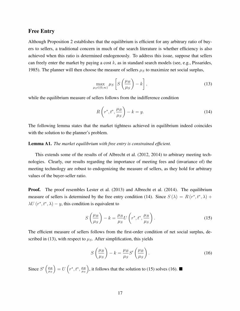
Although Proposition 2 establishes that the equilibrium is efficient for any arbitrary ratio of buy-ers to sellers, a traditional concern in much of the search literature is whether efficiency is alsoachieved when this ratio is determined endogenously. To address this issue, suppose that sellerscan freely enter the market by paying a cost k, as in standard search models (see, e.g., Pissarides,1985). The planner will then choose the measure of sellers µS to maximize net social surplus,

maxµS∈(0,∞)

µS

[S

(µBµS

)− k], (13)

while the equilibrium measure of sellers follows from the indifference condition

R

(r∗, t∗,

µBµS

)− k = y. (14)

The following lemma states that the market tightness achieved in equilibrium indeed coincideswith the solution to the planner’s problem.

Lemma A1. The market equilibrium with free entry is constrained efficient.

This extends some of the results of of Albrecht et al. (2012, 2014) to arbitrary meeting tech-nologies. Clearly, our results regarding the importance of meeting fees and (invariance of) themeeting technology are robust to endogenizing the measure of sellers, as they hold for arbitraryvalues of the buyer-seller ratio.

Proof. The proof resembles Lester et al. (2013) and Albrecht et al. (2014). The equilibriummeasure of sellers is determined by the free entry condition (14). Since S (λ) = R (r∗, t∗, λ) +

λU (r∗, t∗, λ)− y, this condition is equivalent to

S

(µBµS

)− k =

µBµSU

(r∗, t∗,

µBµS

). (15)

The efficient measure of sellers follows from the first-order condition of net social surplus, de-scribed in (13), with respect to µS . After simplification, this yields

S

(µBµS

)− k =

µBµSS ′(µBµS

). (16)

Since S ′(µBµS

)= U

(r∗, t∗, µB

µS

), it follows that the solution to (15) solves (16). �

17

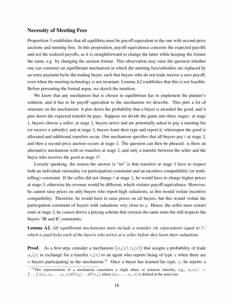
Necessity of Meeting Fees

Proposition 3 establishes that all equilibria must be payoff-equivalent to the one with second-priceauctions and meeting fees. In this proposition, payoff-equivalence concerns the expected payoffsand not the realized payoffs, as it is straightforward to change the latter while keeping the formerthe same, e.g. by changing the auction format. This observation may raise the question whetherone can construct an equilibrium mechanism in which the meeting fees/subsidies are replaced byan extra payment by/to the trading buyer, such that buyers who do not trade receive a zero payoff,even when the meeting technology is not invariant. Lemma A2 establishes that this is not feasible.Before presenting the formal argue, we sketch the intuition.

We know that any mechanism that is chosen in equilibrium has to implement the planner’ssolution, and it has to be payoff equivalent to the mechanism we describe. This puts a lot ofstructure on the mechanism: it pins down the probability that a buyer is awarded the good, and itpins down the expected transfer he pays. Suppose we divide the game into three stages: at stage1, buyers choose a seller; at stage 2, buyers arrive and are potentially asked to pay a meeting fee(or receive a subsidy); and at stage 3, buyers learn their type and report it, whereupon the good isallocated and additional transfers occur. Our mechanism specifies that all buyers pay t at stage 2,and then a second price auction occurs at stage 3. The question can then be phrased: is there analternative mechanism with no transfers at stage 2, and only a transfer between the seller and thebuyer who receives the good at stage 3?

Loosely speaking, the reason the answer is “no” is that transfers at stage 3 have to respectboth an individual rationality (or participation) constraint and an incentive compatibility (or truth-telling) constraint. If the seller did not charge t at stage 2, he would have to charge higher pricesat stage 3; otherwise his revenue would be different, which violates payoff-equivalence. However,he cannot raise prices on only buyers who report high valuations, as this would violate incentivecompatibility. Therefore, he would have to raise prices on all buyers, but this would violate theparticipation constraint of buyers with valuations very close to y. Hence, the seller must extractrents at stage 2; he cannot derive a pricing scheme that extracts the same rents but still respects thebuyers’ IR and IC constraints.

Lemma A2. All equilibrium mechanisms must include a transfer, (in expectation) equal to t∗,

which is paid by/to each of the buyers who arrive at a seller before they learn their valuations

Proof. As a first step, consider a mechanism {φn(x), τn(x)} that assigns a probability of tradeφn(x) in exchange for a transfer τn(x) to an agent who reports being of type x when there aren buyers participating in the mechanism.21 Once a buyer has learned his type, x, he reports a

21This representation of a mechanism constitutes a slight abuse of notation whereby, e.g., φn(x1) =∫. . .∫φ(x1, x2, . . . , xn, n)dF (x2) . . . dF (xn), where φ(x1, . . . , xn, n) is defined in the main text.

18

valuation x′ which maximizesφn (x′)x− τn (x′) . (17)

The incentive compatibility (or truth-telling) constraint then requires

φ′n (x)x− τ ′n (x) = 0. (18)

Hence,

τn (x) =

∫ x

y

τ ′n (x) dx+ C0 =

∫ x

y

xdφn (x) + C0

= φn (x)x− yφn (y)−∫ x

y

φn (x) dx+ C0

= φn (x)x−∫ x

y

φn (x) dx+ C1, (19)

for constants C0 and C1, where the second equality follows from integration by parts. Combining(17) and (19) yields ∫ x

y

φn (x) dx− C1. (20)

Hence, in any incentive compatible mechanism, the expected payoff to a buyer with valuation x iscompletely determined by the probability of trade, φn(x), and a constant C1.

Next, as a second step, we will show that both the probabilities of trade and the constant C1 areuniquely determined in any equilibrium of our game. To see this, first note that any equilibriummechanism must be constrained efficient (Proposition 2 in the text), which implies that the goodmust be allocated to the agent who values it most. Hence,

φn(x) =

F n−1(x) if x ≥ y

0 otherwise.(21)

Substituting (21) into (20) and taking expectations over n and x, we find that the ex ante expectedutility of a buyer is

U =∞∑n=1

Qn (λ)

[∫ x

x

∫ x

y

F n−1 (x) dxdF (x)− C1

]. (22)

By Proposition 3, U = U(r∗, t∗,Λ) in any equilibrium, which implies that C1 is also uniquelydetermined. Indeed, in our mechanism, C1 = t, the meeting fee.

Finally, as a last step, consider an equilibrium of our game in which C1 = t > 0. Moreover,

19

suppose we decompose C1 = Ca1 +Cb

1, where Ca1 denotes any fees that are paid before buyers learn

their type, and Cb1 are transfers made after reporting x. The individual rationality (or participation)

constraint of a buyer with valuation x is given by∫ x

y

φn (x) dx− Cb1 ≥ 0. (23)

Since this constraint must hold for all x ∈ [y, x], it follows that Cb1 = 0 in every equilibrium. �

Restrictions on M

Our assumptions about Pn (λ) and m (z;λ) impose a number of restrictions on M (·).22

(i) m being a probability-generating function requires that M is an analytic function.23

(ii) 1n!

∂n

∂znm (0;λ) ∈ [0, 1] for all n and all λ requires that (−λ)n

n!M (n) (λ) ∈ [0, 1] for all n and λ;

(iii) m (1;λ) = 1 for all λ requires that M (0) = 1;

(iv) mz (1;λ) ∈ [0, λ] for all λ requires that M ′ (0) ∈ [−1, 0];

(v) mλ (z;λ) < 0 for all z and all λ requires that M ′ (λ) < 0 for all λ;

(vi) mλλ (z;λ) > 0 for all z and all λ requires that M ′′ (λ) > 0 for all λ.

Jointly, these restrictions completely characterize the set of feasible M (·). However, a tightercharacterization is possible. For example, restriction (ii) can be tightened as follows

(ii′) M satisfies (−λ)n

n!M (n) (λ) ∈ (0, 1) for all n and λ.

Proof. We provide a proof by contradiction. Suppose that there exist a n ∈ N0 and a λ > 0 such

that (−λ)n

n!M (n)

(λ)

= 0. As λ > 0, this impliesM (n)(λ)

= 0. BecauseM (n) (λ) is continuously

differentiable but cannot cross zero, it must be the case that its first derivative is zero in λ = λ aswell, i.e. M (n+1)

(λ)

= 0. By induction, it then follows that all higher derivatives must equal zero

in this point, M (n)(λ)

= 0 for all n ∈ {n, n+ 1, n+ 2, . . .}.

With all of its derivatives being zero in λ, the analytic function M (n) (λ) must be zero ina neighborhood around λ. Again by induction, we therefore obtain that M (n) (λ) = 0 for all

22To keep notation concise, we write “all λ” instead of “all λ ∈ (0,∞)”, “all n instead of “all n ∈ N0”, and “all z”instead of “all z ∈ [0, 1)”.

23Probability-generating functions are analytic functions (Sachkov, 1997).

20

n ∈ {n, n+ 1, n+ 2, . . .} and all λ. In that case,

n−1∑i=0

Pi (λ) =n−1∑i=0

(−λ)i

i!M (i) (λ) = 1,

which is a differential equation with solution M (λ) = 1 +∑n−1

i=1 ciλi, for some coefficients

ci. Because M ′ (λ) < 0 rules out the possibility that M (λ) is a constant, one obtains thatlimλ→∞ |M (λ)| = +∞.

This contradicts the requirement that M (λ) ∈ [0, 1] for all λ. Hence, it must be true that(−λ)n

n!M (n) (λ) > 0 for all n and all λ. This immediately implies that (−λ)n

n!M (n) (λ) < 1, for all n

and all λ, which completes the proof. �

Note that restriction (ii′) implies restriction (v) and (vi), which are therefore redundant. Hence,the set of feasible M can be characterized by restrictions (i), (ii′), (iii), and (iv).

Independence

Another well-known property of the urn-ball meeting technology is that Pn (λ) does not onlyrepresent the distribution of the total number of buyers at each seller, but also the distribution ofthe number of competitors a buyer faces when arriving at a seller. In other words, a buyer whomeets with a seller has no effect on the distribution (and thus the expectation) of the number ofother buyers at the same seller. We will say that a meeting technology that satisfies this propertyexhibits “independence”.

Formally, independence means Qn (λ) = (1−Q0 (λ))Pn−1 (λ) for all λ and n ∈ N1. Thisproperty can be shown to be satisfied if and only if the meeting technology is of the followingform:24

Pn (λ) = e−(1−Q0(λ))λ [(1−Q0 (λ))λ]n

n!. (24)

The following lemma establishes that independence is neither a necessary nor a sufficient conditionfor invariance.

Lemma 3. Invariance does not imply independence and independence does not imply invariance.

To see why invariance does not imply independence, consider the geometric technology. Aswe established in the main text, this meeting technology is invariant. However, this technology isnot independent, as the fact that an individual buyer meets with a seller changes the probability

24By the consistency requirement and induction, the condition implies that Pn (λ) = 1n!λ

n [1−Q0 (λ)]nP0 (λ) .

Since Pn (λ) is a probability distribution, we must have 1 =∑∞

01n!λ

n [1−Q0 (λ)]nP0 (λ) = eλ[1−Q0(λ)]P0 (λ) .

Solving the second equation for P0 (λ) and substituting the solution into the first equation yields (24). Conversely,equation (24) implies the independence condition immediately.

21

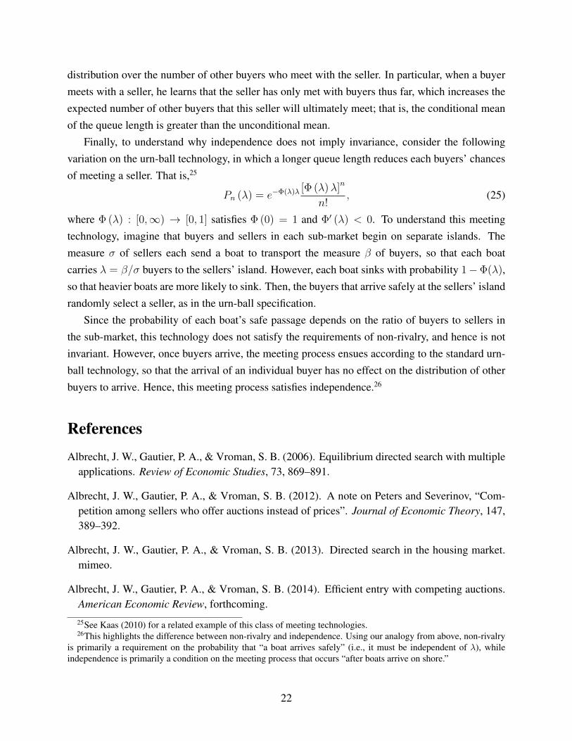
distribution over the number of other buyers who meet with the seller. In particular, when a buyermeets with a seller, he learns that the seller has only met with buyers thus far, which increases theexpected number of other buyers that this seller will ultimately meet; that is, the conditional meanof the queue length is greater than the unconditional mean.

Finally, to understand why independence does not imply invariance, consider the followingvariation on the urn-ball technology, in which a longer queue length reduces each buyers’ chancesof meeting a seller. That is,25

Pn (λ) = e−Φ(λ)λ [Φ (λ)λ]n

n!, (25)

where Φ (λ) : [0,∞) → [0, 1] satisfies Φ (0) = 1 and Φ′ (λ) < 0. To understand this meetingtechnology, imagine that buyers and sellers in each sub-market begin on separate islands. Themeasure σ of sellers each send a boat to transport the measure β of buyers, so that each boatcarries λ = β/σ buyers to the sellers’ island. However, each boat sinks with probability 1−Φ(λ),so that heavier boats are more likely to sink. Then, the buyers that arrive safely at the sellers’ islandrandomly select a seller, as in the urn-ball specification.

Since the probability of each boat’s safe passage depends on the ratio of buyers to sellers inthe sub-market, this technology does not satisfy the requirements of non-rivalry, and hence is notinvariant. However, once buyers arrive, the meeting process ensues according to the standard urn-ball technology, so that the arrival of an individual buyer has no effect on the distribution of otherbuyers to arrive. Hence, this meeting process satisfies independence.26

References

Albrecht, J. W., Gautier, P. A., & Vroman, S. B. (2006). Equilibrium directed search with multipleapplications. Review of Economic Studies, 73, 869–891.

Albrecht, J. W., Gautier, P. A., & Vroman, S. B. (2012). A note on Peters and Severinov, “Com-petition among sellers who offer auctions instead of prices”. Journal of Economic Theory, 147,389–392.

Albrecht, J. W., Gautier, P. A., & Vroman, S. B. (2013). Directed search in the housing market.mimeo.

Albrecht, J. W., Gautier, P. A., & Vroman, S. B. (2014). Efficient entry with competing auctions.American Economic Review, forthcoming.

25See Kaas (2010) for a related example of this class of meeting technologies.26This highlights the difference between non-rivalry and independence. Using our analogy from above, non-rivalry

is primarily a requirement on the probability that “a boat arrives safely” (i.e., it must be independent of λ), whileindependence is primarily a condition on the meeting process that occurs “after boats arrive on shore.”

22

Burdett, K., Shi, S., & Wright, R. (2001). Pricing and matching with frictions. Journal of PoliticalEconomy, 109, 1060–1085.

Butters, G. (1977). Equilibrium distributions of sales and advertising prices. Review of EconomicStudies, 44(3), 465–491.

Duffie, D., Garleanu, N., & Pedersen, L. H. (2007). Valuation in over-the-counter markets. Reviewof Financial Studies, 20(6), 1865–1900.

Eeckhout, J. & Kircher, P. (2010). Sorting vs screening - search frictions and competing mecha-nisms. Journal of Economic Theory, 145, 1354–1385.

Galenianos, M. & Kircher, P. (2009). Directed search with multiple job applications. Journal ofEconomic Theory, 114, 445–471.

Hall, R. (1977). Microeconomic Foundations of Macroeconomics, chapter An Aspect of the Eco-nomic Role of Unemployment. Macmillan, London.

Harremoes, P., Johnson, O., & Kontoyiannis, I. (2010). Thinning, entropy, and the law of thinnumbers. IEEE Transactions on Information Theory, 56(9), 4228–4244.

Hosios, A. K. (1990). On the efficiency of matching and related models of search and unemploy-ment. Review of Economic Studies, 57, 279–298.

Kaas, L. (2010). Variable search intensity in an economy with coordination unemployment. B.E.Journal of Macroeconomics, 10(1), 1–33.

Kim, K. & Kircher, P. (2013). Efficient competition through cheap talk: Competing auctions andcompetitive search without ex-ante commitment. CEPR Discussion Paper DP9785.

Kircher, P. (2009). Efficiency of simultaneous search. Journal of Political Economy, 117, 861–913.

Kiyotaki, N. & Wright, R. (1993). A search-theoretic approach to monetary economics. AmericanEconomic Review, 83(1), 63–77.

Lester, B., Visschers, L., & Wolthoff, R. P. (2013). Competing with asking prices. Federal ReserveBank of Philadelphia Working Paper 13-7.

Moen, E. R. (1997). Competitive search equilibrium. Journal of Political Economy, 105, 385–411.

Mortensen, D. T. (1982). Efficiency of mating, racing, and related games. American EconomicReview, 72, 968–979.

Peters, M. (1997). A competitive distribution of auctions. The Review of Economic Studies, 64(1),97–123.

23

Peters, M. (2010). Noncontractible heterogeneity in directed search. Econometrica, 78(4), 1173–1200.

Peters, M. (2013). Competing mechanisms. In N. Vulcan, A. Roth, & Z. Neeman (Eds.), TheHandbook of Market Design. Oxford University Press.

Peters, M. & Severinov, S. (1997). Competition among sellers who offer auctions instead of prices.Journal of Economic Theory, 75, 141–179.

Pissarides, C. A. (1985). Short-run equilibrium dynamics of unemployment, vacancies and realwages. American Economic Review, 75, 676–690.

Renyi, A. (1956). A characterization of Poisson processes. Magyar Tud. Akad. Mat. Kutalo Int.Kozl., 1, 519–527.

Sachkov, V. (1997). Probabilistic Methods in Discrete Mathematics, volume 56 of Encyclopediaof Mathematics and its Applications. New York: Cambridge University Press.

Shi, S. (2001). Frictional assignment I: Efficiency. Journal of Economic Theory, 98(2), 232–260.

Shimer, R. (2005). The assignment of workers to jobs in an economy with coordination frictions.Journal of Political Economy, 113(5), 996–1025.

Trejos, A. & Wright, R. (1995). Search, bargaining, money, and prices. Journal of PoliticalEconomy, 103(1), 118–141.

Virag, G. (2010). Competing auctions: Finite markets and convergence. Theoretical Economics,5, 241–274.

Wolthoff, R. P. (2012). Applications and interviews: A structural analysis of two-sided simultane-ous search. FEEM Working Paper 637.

24