
Sinan Gemici, Patrick Lim and Tom Karmel, NCVER · Web viewThe lower-level nodes display...
78
The impact of schools on young people’s transition to university Sinan Gemici Patrick Lim Tom Karmel NCVER FOR CLARITY WITH FIGURES PLEASE PRINT IN COLOUR The views and opinions expressed in this document are those of the author/ project team and do not necessarily reflect the views of the Australian Government, state and territory governments or NCVER. Any interpretation of data is the responsibility of the LONGITUDINAL SURVEYS OF AUSTRALIAN YOUTH RESEARCH REPORT 61
Transcript of Sinan Gemici, Patrick Lim and Tom Karmel, NCVER · Web viewThe lower-level nodes display...

The impact of schools on young people’s transition to university
Sinan GemiciPatrick LimTom KarmelNCVER
FOR CLARITY WITH FIGURESPLEASE PRINT IN COLOUR
The views and opinions expressed in this document are those of the author/project team and do not necessarily reflect the views of the Australian Government, state and territory governments or NCVER.
Any interpretation of data is the responsibility of the author/project team.
LONGITUDINAL SURVEYS OF AUSTRALIAN YOUTHRESEARCH REPORT 61

© Commonwealth of Australia, 2013
With the exception of the Commonwealth Coat of Arms, the Department’s logo, any material protected by a trade mark and where otherwise noted all material presented in this document is provided under a Creative Commons Attribution 3.0 Australia <http://creativecommons.org/licenses/by/3.0/au> licence.
The details of the relevant licence conditions are available on the Creative Commons website (accessible using the links provided) as is the full legal code for the CC BY 3.0 AU licence <http://creativecommons.org/licenses/by/3.0/legalcode>.
The Creative Commons licence conditions do not apply to all logos, graphic design, artwork and photographs. Requests and enquiries concerning other reproduction and rights should be directed to the National Centre for Vocational Education Research (NCVER).
This document should be attributed as Gemici, S, Lim, P & Karmel, T 2013, The impact of schools on young people’s transition to university, NCVER, Adelaide.
This work has been produced by NCVER through the Longitudinal Surveys of Australian Youth (LSAY) Program, on behalf of the Australian Government and state and territory governments, with funding provided through the Australian Department of Education, Employment and Workplace Relations.
ISBN 978 1 922056 24 5
TD/TNC 109.16
Published by NCVERABN 87 007 967 311
Level 11, 33 King William Street, Adelaide SA 5000PO Box 8288 Station Arcade, Adelaide SA 5000, Australia
P +61 8 8230 8400 F +61 8 8212 3436 E [email protected] W <http://www.ncver.edu.au>
About the research
The impact of schools on young people’s transition to university
Sinan Gemici, Patrick Lim and Tom Karmel, NCVERThe Longitudinal Surveys of Australian Youth (LSAY), in addition to the characteristics of the individual students making up the sample, collect data on a range of school characteristics. This, and the fact that the sample is clustered with the selected schools as the first stage, provides the opportunity to disentangle the impact of the school from the characteristics of students. This report exploits this feature of LSAY to investigate the impact of schools on tertiary entrance rank (TER) and the probability of going to university. While secondary education is about more than these academic goals, there is no doubt that these are of high importance, both from the point of view of the schools and the individual students and their parents.
The school characteristics covered in this report are: simple characteristics, such as school sector and location; structural characteristics, such as whether the school is single-sex or coeducational; resource base, such as class size and student—teacher ratio; and average demographics, such as the average socioeconomic status of students at the school and the extent to which parents put pressure on the school to achieve high academic results.
Key messages The attributes of schools do matter. Although young people’s individual characteristics
are the main drivers of success, school attributes are responsible for almost 20% of the variation in TER.
Of the variation in TER attributed to schools, the measured characteristics account for a little over a third. The remainder captures ‘idiosyncratic’ school factors that cannot be explained by the data to hand and that can be thought of as a school’s overall ‘ethos’; no doubt teacher quality and educational leadership are important here.
The three most important school attributes for TER are sector (that is, Catholic and independent vs government), gender mix (that is, single-sex vs coeducational), and the extent to which a school is ‘academic’. For TER, the average socioeconomic status of students at a school does not emerge as a significant factor, after controlling for individual characteristics including academic achievement from the PISA test.
However, the characteristics of schools do matter for the probability of going to university, even after controlling for TER. Here, the three most important school attributes are the proportion of students from non-English speaking backgrounds, sector, and the school’s socioeconomic make-up.
The authors also construct distributions of school performance (in relation to TER and the probability of going to university), which control for individual characteristics. The differences between high-performing and low-performing schools are sizeable. There is also considerable variation within school sectors, with the government sector having more than its share of low-performing schools.

Tom KarmelManaging Director, NCVER

ContentsTables and figures 6
Executive summary 8
Introduction 10
Current knowledge about school effects in Australia 11
Analysis 13Data and sample 13Multi-level modelling 16
Results 17TER 17Further exploration of influential school attributes 26Comparing influential school attributes against performance 29Differentiating the impact of schools by cluster 33
Conclusion 36
References 37
Appendices
A: Descriptive statistics 39
B: Student-level measures 42
C: Factor analysis for SES measure 44
D: Factor analysis for perceptions of schooling measure 46
E: Technical details on multi-level modelling 48
F: Results from multi-level modelling 50
G: Information on the Logistic scale 57
6 The impact of schools on young people’s transition to university
Tables and figuresTables1 Summary of school effects research in Australia 122 Results for school-level predictors of TER 183 Results for school-level predictors of university enrolment after
accounting for TER 224 Combined statistically significant school attributes by cluster 305 Academic and instructional/religious selection criteria 316 Sources of funding by sector and cluster 327 Geographic distribution of schools by sector 328 Geographic distribution of schools by performance cluster 33A1 Descriptive statistics for student-level predictors (unweighted) 39A2 Descriptive statistics for school-level predictors (unweighted) 40A3 Descriptive statistics for outcome variables (unweighted) 41C1 Eigenvalues for SES factor analysis 44C2 One-factor model for SES measure 45D1 Eigenvalues for perceptions of schooling factor analysis 46D2 One-factor model for perceptions of schooling measure 47F1 Variance components for null and final models across outcomes 50F2 Results for student-level predictors of TER 51F3 Results for school-level predictors of TER 52F4 Results for student-level predictors of university enrolment 54F5 Results for school-level predictors of university enrolment 55G1 Conversion table of logistic scale to linear predictor 57
Figures1 Variation accounted for by student versus school-level
characteristics (%) 172 Explained school-level variation for TER after multi-level modelling213 Distribution of school idiosyncratic effects on TER 214 Tree diagram for TER 245 Tree diagram for university enrolment 256 Caterpillar plots of between-school differences for TER after multi-
level modelling 277 Caterpillar plots of between-school differences for university
enrolment after multi-level modelling 288 Cluster analysis of school performance 29
NCVER 7
9 Components of total TER effect by cluster 3410 Components of total university enrolment effect by cluster 35C1 Scree plot from SES factor analysis 45D1 Scree plot from perceptions of schooling factor analysis 47G1 Conversion graph of logistic scale to linear predictor 57
8 The impact of schools on young people’s transition to university
Executive summaryThis report uses data from the 2006 cohort of the Longitudinal Surveys of Australian Youth (LSAY) to investigate how schools influence tertiary entrance rank1 (TER) and university enrolment over and above young people’s individual background characteristics. A particular focus is on prominent school-level factors such as sector, school demographic make-up, resources and autonomy, academic orientation, and competition with other schools.
The analysis finds that, while the impact of individual student characteristics is dominant with respect to TER and the transition to university, the way in which schools are organised and operated also matters. And it matters for the probability of going to university, even after controlling for individual TER and other relevant background factors. Of the 25 school characteristics included in the analysis, ten attributes significantly influence either TER or university enrolment, or both. The three most important attributes for TER include school sector (Catholic and independent schools have higher predicted TERs than government schools), gender mix (single-sex schools have higher predicted TERs than coeducational schools), and the extent to which a school is academically oriented.
The role of a school’s overall socioeconomic status with respect to TER is interesting. Previous studies have found that a school’s overall socioeconomic status affects academic achievement outcomes in NAPLAN and PISA. The present study finds that a school’s overall socioeconomic status does not influence students’ TER outcomes, after controlling for individual characteristics including academic achievement from the PISA test. However, the socioeconomic make-up of the student body does influence the probability of going on to university for a given TER. Two other school attributes also affect university enrolment after controlling for individual TER: a high proportion of students from non-English speaking backgrounds and school sector.
After isolating influential school attributes, cluster analysis is used to identify three groups of schools: high-performance schools, where a school’s attributes contribute to a high TER and a high probability of going to university (after controlling for TER); low-performance schools at the other end of the spectrum; and average-performance schools that show middling performance.2 Although after controlling for relevant characteristics, the high-performance cluster includes schools from all three sectors, the low-performing schools are almost all from the government sector. Academic orientation, as measured through parental pressure for the school to perform well academically is important, as are the limitations imposed by the timetable of work-related programs. Schools that deviate from the norm (single-sex schools, the small number of schools that do not see themselves as competing with other schools and the few which stream either all or no subjects) perform better than average, as do those with high proportions of students from language backgrounds other than English. The analysis further shows that resources do have some impact. On average, schools with lower student—teacher ratios obtain slightly better TERs,
1 At present, the Australian Tertiary Admission Rank (ATAR) is used as a nationwide university entrance score. However, at the time of data collection respondents reported state-based tertiary entrance rank (TER) or equivalent scores. The term ‘TER’ is used throughout this report to denote respondents’ university entrance scores.
2 The performance measure used controls for individual student characteristics.
NCVER 9

and student fees contribute more to school funds among schools in the high-performing cluster.
Many high-performing schools also have positive ‘idiosyncratic’ factors that contribute to high TERs. This term is used throughout the paper to denote aspects of an individual school’s performance that can be identified statistically but which cannot be explained further using the LSAY data. Idiosyncratic effects reflect a given school’s overall ‘ethos’, which has an important influence on individual student achievement.
Schools in the low-performance group have measured attributes that are not conducive to high TERs, as well as negative idiosyncratic traits. This picture is complicated by the fact that some low-performing schools have students who are likely to do well regardless of the school’s particular characteristics, just as some high-performing schools will have students who get low TERs. Overall, the magnitudes of the differences are sizeable, in that the measured school attributes of high-performing schools add ten to 15 points to the average TER compared with the low-performing schools. While school idiosyncratic effects have a small positive effect on most high-performing schools, their impact on low-performing schools can be quite detrimental.
With respect to university enrolment, measured school characteristics in high-performing schools generally have a positive impact on university enrolment, and an increasingly negative impact as school performance diminishes. Compared with the effect realised through TER, however, young people’s individual characteristics play a much stronger role with respect to university enrolment than the characteristics of their schools, regardless of the performance cluster.
10 The impact of schools on young people’s transition to university
IntroductionIndividual background characteristics, such as academic ability, educational aspirations or parental background, can have a tremendous impact on the probability of a young person going to university. However, a successful transition to higher education is not determined by individual circumstances alone. Schools themselves play an important role in the way in which they allocate resources, select students and support a positive learning environment. Organisational and demographic factors such as school sector, size, geographic location and the socioeconomic profile of the student body further affect key education and transition outcomes.
When considering the impact of schools on student outcomes, it is important to separate the effect of school characteristics from that of young people’s individual background factors. It is also necessary to take into account that students who attend the same school are generally more similar to each other than to students who attend a different school. For example, it is quite likely that going to a school where most students aspire to go to university will impact on an individual student’s decision to pursue a degree. Multi-level analysis, which is able to properly handle such complexities, is used in this study to determine which school attributes influence TER and university enrolment over and above young people’s individual characteristics.
A number of studies have provided valuable insights into influential school characteristics, yet no consistent picture has emerged about which particular school attributes really matter for university-bound youth. This report seeks to shed light on this question by exploring different aspects of schools and how they impact on young people’s transition to higher education. Specifically, it uses data from the 2006 cohort of the Longitudinal Surveys of Australian Youth (LSAY) to examine which school characteristics have a significant influence on TER and university enrolment by age 19.
The report proceeds as follows. The first section presents a brief stocktake of what is currently known about influential school characteristics in Australia. The two subsequent sections provide an outline of the analysis and the results of the modelling. Section four contains a brief conclusion.
NCVER 11

Current knowledge about school effects in AustraliaFullarton (2002) examined the relationship between school characteristics and students’ engagement in their education. Her study showed that 9% of the variation in young people’s engagement in their education was due to differences between schools. She further found that the negative effects of low socioeconomic status and poor self-assessment of ability were moderated by schools that created a better learning climate and offered a broader range of extracurricular activities. Overall, Fullarton concluded that, with respect to student engagement, it did matter which school a child attended.
The availability of mathematics and reading achievement scores from the Programme for International Student Assessment (PISA)3 prompted Rothman and McMillan’s (2003) investigation of school-level influences on numeracy and literacy. The authors determined that differences in school attributes accounted for approximately 16% of the variation in mathematics and reading scores. Over half of this variation could be explained by the average socioeconomic status of a school’s student body, school climate (a composite variable that aggregates students’ perceived quality of school life to the school level), and the proportion of students from language backgrounds other than English.
The extent to which schools facilitate the completion of Year 12 has received considerable attention from researchers. A study by Le and Miller (2004) suggested that, while schools did have an effect on Year 12 completion, this effect was more strongly related to ‘the selection of more able students with superior socioeconomic backgrounds than with the independent creation of favourable school or classroom climates’ (p.194). In a similar vein, Marks (2007) determined that schools did not have a strong independent influence on Year 12 completion, once the effects of individual student characteristics were taken into account.
Curtis and McMillan (2008) also considered school effects on Year 12 completion and found that school climate factors, such as poor student—teacher relationships, low teacher morale and poor student behaviour contribute to early school leaving. These findings were contrary to those of Marks (2007), who concluded that there were few schools with substantially higher or lower levels of Year 12 completion than expected, given their students’ individual characteristics, and that these schools did not differ from other schools in identifiable, systematic ways.
Marks (2010a) also examined the effect of school characteristics on TER. In contrast with prior work by Fullarton (2002) and Rothman and McMillan (2003), he found a rather modest independent school effect. He ascertained moderate effects for the extent to which parents pressured schools for academic excellence, disciplinary climate, average school achievement scores and teaching quality. Neither of Marks’s studies, however, determined a significant effect for the average socioeconomic status of a school’s student body after accounting for individual background characteristics.
3 PISA is auspiced by the Organisation for Economic Co-operation and Development (OECD).
12 The impact of schools on young people’s transition to university
Two recent studies have further intensified research into schools and their characteristics. The first study (OECD 2010) carried out an international benchmarking exercise to determine school effects on PISA 2009 reading scores. For Australia, the absence of student selection criteria, high levels of school control over curriculum and assessment, and higher teacher salaries were found to have a significant positive effect on reading performance. The average socioeconomic status of a school’s student body accounted for almost 13% of the variation in reading scores between schools.
The second study (NOUS Group et al. 2011) focused on academic ability and equity within the Australian school system. Results from PISA 2009 data corroborated findings from previous studies (for example, Le & Miller 2004; Marks 2007, 2010a), in that individual student factors, and most notably academic performance, had a far larger impact on student outcomes than the characteristics of a given school. The report concluded that what did matter at the school level were teaching effectiveness and a positive classroom climate, strong school leadership, school resources and the school’s reputation within its community. Table 1 provides a summary of selected research on school effects in Australia.
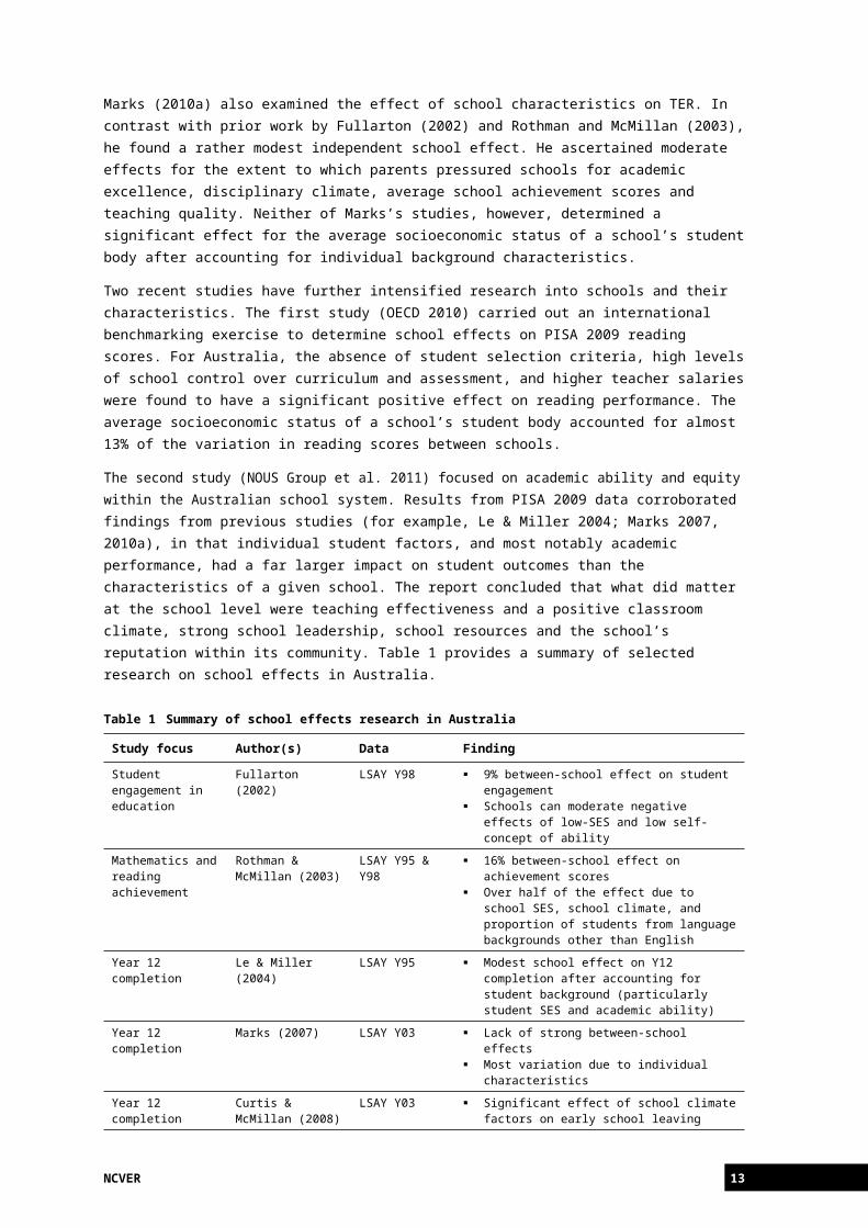
Table 1 Summary of school effects research in Australia
Study focus Author(s) Data Finding
Student engagement in education
Fullarton (2002) LSAY Y98 9% between-school effect on student engagement
Schools can moderate negative effects of low-SES and low self-concept of ability
Mathematics and reading achievement
Rothman & McMillan (2003)
LSAY Y95 & Y98 16% between-school effect on achievement scores
Over half of the effect due to school SES, school climate, and proportion of students from language backgrounds other than English
Year 12 completion Le & Miller (2004) LSAY Y95 Modest school effect on Y12 completion after accounting for student background (particularly student SES and academic ability)
Year 12 completion Marks (2007) LSAY Y03 Lack of strong between-school effects Most variation due to individual characteristics
Year 12 completion Curtis & McMillan (2008)
LSAY Y03 Significant effect of school climate factors on early school leaving
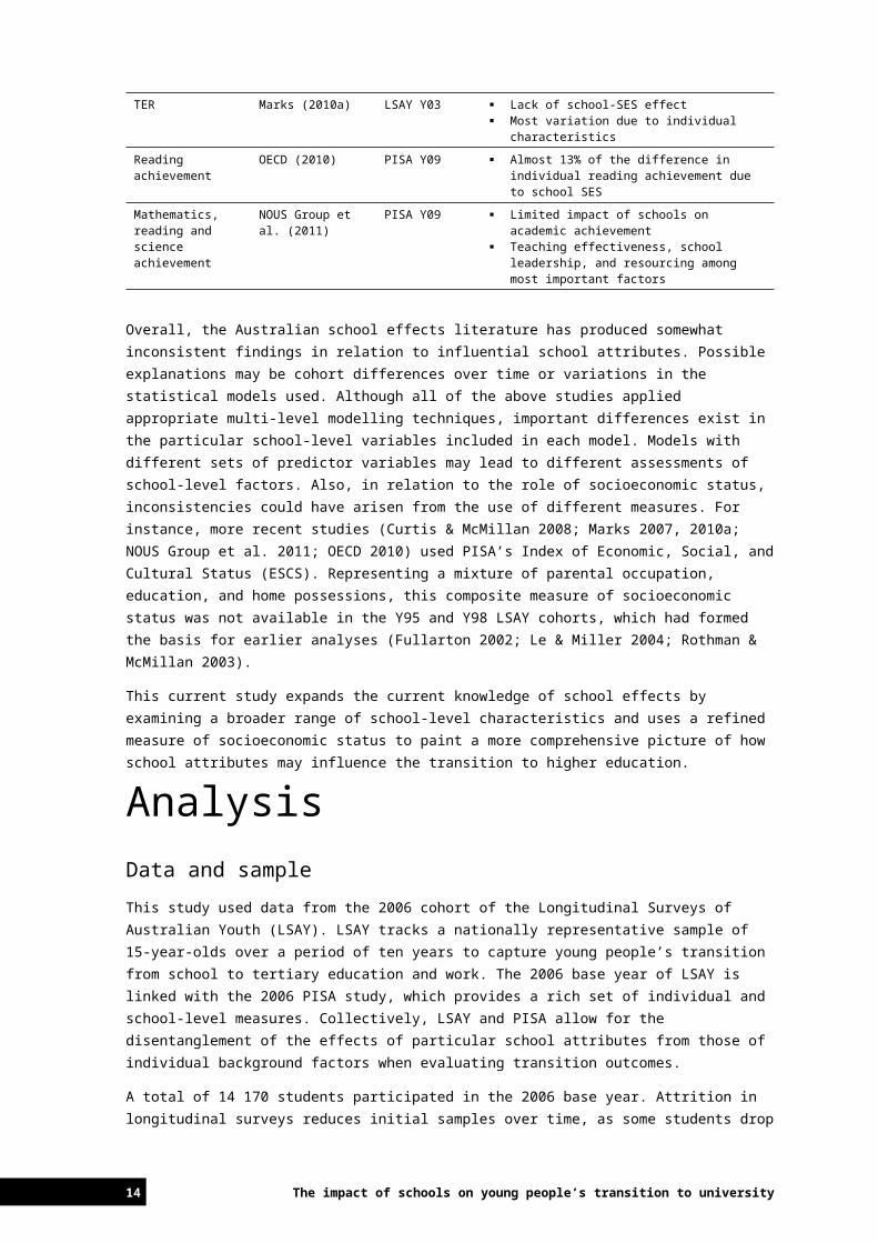
TER Marks (2010a) LSAY Y03 Lack of school-SES effect Most variation due to individual characteristics
Reading achievement
OECD (2010) PISA Y09 Almost 13% of the difference in individual reading achievement due to school SES
Mathematics, reading and science achievement
NOUS Group et al. (2011)
PISA Y09 Limited impact of schools on academic achievement
Teaching effectiveness, school leadership, and resourcing among most important factors
Overall, the Australian school effects literature has produced somewhat inconsistent findings in relation to influential school attributes. Possible explanations may be cohort differences over time or variations in the statistical models used. Although all of the above studies applied appropriate multi-level modelling techniques, important differences exist in the particular school-level variables included in each model. Models with different sets of predictor variables may lead to different assessments of school-level factors. Also, in relation to the role of socioeconomic status, inconsistencies could have arisen from the use of different measures. For instance, more recent studies (Curtis & McMillan 2008; Marks 2007, 2010a; NOUS Group et al. 2011; OECD 2010) used PISA’s Index of Economic, Social, and Cultural Status (ESCS). Representing a mixture of parental occupation, education, and
NCVER 13
home possessions, this composite measure of socioeconomic status was not available in the Y95 and Y98 LSAY cohorts, which had formed the basis for earlier analyses (Fullarton 2002; Le & Miller 2004; Rothman & McMillan 2003).
This current study expands the current knowledge of school effects by examining a broader range of school-level characteristics and uses a refined measure of socioeconomic status to paint a more comprehensive picture of how school attributes may influence the transition to higher education.
AnalysisData and sampleThis study used data from the 2006 cohort of the Longitudinal Surveys of Australian Youth (LSAY). LSAY tracks a nationally representative sample of 15-year-olds over a period of ten years to capture young people’s transition from school to tertiary education and work. The 2006 base year of LSAY is linked with the 2006 PISA study, which provides a rich set of individual and school-level measures. Collectively, LSAY and PISA allow for the disentanglement of the effects of particular school attributes from those of individual background factors when evaluating transition outcomes.
A total of 14 170 students participated in the 2006 base year. Attrition in longitudinal surveys reduces initial samples over time, as some students drop out for a variety of reasons (see Rothman 2009). All students who were still part of the LSAY sample in 2010 (n = 6315) were included in the analysis. To ascertain school-level effects on TER, a sub-sample of only those students who reported a valid TER (n = 3797) was also created.
In addition to student-level data, the 2006 PISA school questionnaire collected information from school administrators on a variety of factors that may influence school performance. School-level data were collected on a representative sample of 356 Australian schools in the 2006 base year.4 Appropriate weights were applied to the student and school samples to correct for the effects of complex sampling and attrition. Interested readers can find details on these weights in Lim (2011) and OECD (2009). The next section discusses the outcome and student- and school-level measures used in this study. Descriptive statistics for all measures are provided in appendix A.
Outcome measuresThe two outcomes examined in this study comprise TER and commencement of a bachelor’s or higher degree (referred to as university enrolment). For TER, all students with valid scores reported by 2010 were included.5 The second outcome measure, university enrolment, captured whether students had ever commenced a bachelor’s or higher degree by 2010. The analyses of university enrolment explicitly controlled for individual TER. Doing so has an important bearing on the interpretation of analysis results because the impact of school attributes on university enrolment is captured over and above the effect of an individual’s TER.
4 A school with a single student response was removed from the data because it had an undue influence on results.
5 An appropriate score conversion was made for Queensland Overall Position scores (see Queensland Tertiary Admissions Centre 2011).
14 The impact of schools on young people’s transition to university
Given that university enrolment was measured when most young people in the sample were 19 years of age, the impact of ‘gap year takers’ on results is unclear. According to Lumsden and Stanwick (2012), 24% of Year 12 completers took gap years in 2009—10.
NCVER 15
Student-level measuresIn order to determine the impact of school attributes on outcome measures, the individual background characteristics of students need to be properly accounted for. Relevant individual background characteristics can be categorised into socio-demographic factors, academic achievement, educational aspirations and students’ overall perceptions of schooling.
Student-level measures included in the analysis are gender, Indigenous status, length of in-country residence, language spoken at home, socioeconomic status, academic achievement at age 15, aspirations for tertiary education and perceptions of the school experience. Details on student-level measures are provided in appendix B.
School-level measuresSchools influence student outcomes through a range of demographic, institutional, and environmental factors. It is also well established that the quality of teachers and teaching practices has a strong impact on student outcomes (see Hattie 2009). Given that teacher and teaching quality is not well captured in the PISA and LSAY data, this aspect is not included in the set of school-level variables as a separate measure. However, it is important to note that academic quality aspects are captured as part of ‘idiosyncratic’ factors (that is, aspects of an individual school’s performance which can be identified statistically but cannot be explained further using the LSAY data). The school-level measures included in the present analysis are briefly outlined in turn.
School sectorSchools are categorised as coming from the government, Catholic and independent sectors.
LocationSchools are divided into those in metropolitan areas and those in non-metropolitan areas.
School demographicsSchool demographics include school size and the make-up of the student body. The latter contains attributes such as the average socioeconomic status and average academic achievement level of a school’s student body, whether the school is coeducational or single sex, as well as the proportion of enrolled students from language backgrounds other than English (LBOTE).6 Apart from size, these variables are constructed from the sample of students in LSAY.
Resources and capacityProxies for school resources include class size, student—teacher ratio and the presence of teacher shortages. In addition, the proportion of certified and highly qualified (that is, above bachelor degree level) teachers per school, indicators capturing a school’s primary resource base7 (that is, whether a school is resourced primarily through government or 6 The LBOTE measure was aggregated to the school level from individual respondents’ declared home
language (that is, ‘English’ or ‘language other than English’).7 The primary resource base measure is derived from the PISA 2006 school questionnaire. In the
questionnaire, principals are asked to report the percentage of school total funding that comes from the
16 The impact of schools on young people’s transition to university

non-government funds) and the quality of educational materials available to the school are considered here.
Academic orientationAcademic orientation consists of a number of variables, such as the intensity with which parents pressure schools to set high academic standards, a school’s consideration of student selection criteria,8 and the use of streaming9 (that is, within grades, the grouping of students by ability level). Also included is the extent to which the school offers participation in school-organised vocational education and training (VET) programs.10 (The authors speculate that the more academic schools either do not offer school-organised VET, or only offer it to a minority of students.)
School autonomySchool autonomy has been defined as ‘a form of school management in which schools are given decision-making authority over their operations, including the hiring and firing of personnel, and the assessment of teachers and pedagogical practices’ (Barrera, Fasih & Patrinos 2009, p.2). It is unclear whether higher levels of school autonomy may result in stronger accountability, which in turn would yield better student outcomes (Bruns, Filmer & Patrinos 2011; Levin 2008). School autonomy included indicators for the level of responsibility that schools are afforded in controlling resources and shaping the curriculum,11 along with a measure of the degree to which businesses in the community influence the school curriculum.
Providing for student needsA school’s ability to create a positive learning environment by providing for student needs may influence educational and post-school transition outcomes. The measures used here include the provision of extracurricular activities, a variable indicating whether the responsibility for career guidance rested with teachers or career counsellors, and a perception of schooling variable that was aggregated from the corresponding student-level variable.
Competitiongovernment, student fees and other sources. Here, a school was considered to be primarily government funded if 50% or more of the funding was reported to come from government.
8 The index of academic selectivity (SELSCH) was derived from school principals’ responses on how much consideration was given to the following factors when students were admitted to the school, based on a scale from the response categories ‘not considered’, ‘considered’, ‘high priority’ and ‘prerequisite’ of items 19b and 19c in the school questionnaire: student’s record of academic performance (including placement tests); and recommendation of feeder schools. This index has the following four categories: (1) schools where neither of the two factors is considered for student admittance, (2) schools considering at least one of these two factors, (3) schools where at least one of these two factors is a high priority for student admittance, and (4) schools where at least one of these two factors is a prerequisite for student admittance. For statistical reasons, the categories ‘at least one of these two factors considered’ and ‘at least one of these two factors is high priority’ were combined.
9 The streaming variable captures whether a school uses streaming in some, all, or no subjects. This variable had limitations, in that the overwhelming majority of schools streamed for some subjects.
10 The exact question to principals is as follows: ‘In your school, about how many students ... receive some training within local businesses as part of school activities during the normal school year (e.g. apprenticeships)?’.
11 The measure of a school’s responsibility over resources was created from items SC11QA1—SC11QF4 in the PISA school questionnaire. The measure of a school’s responsibility over the curriculum was created from items SC11QG1—SC11QL4 in the PISA school questionnaire. Details on deriving autonomy measures are provided in OECD (2010).
NCVER 17
Some ambiguity exists over the impact of competition between schools on school outcomes. While school competition has been linked to higher student achievement in Canada (Card, Dooley & Payne 2010), a general benefit from increased school competition across the developed world has not been ascertained (OECD 2010). In Australia, competition between schools can be problematic because it often reinforces socioeconomic status and performance stratification (Lamb 2007). NOUS Group et al. (2011) point out that the movement of a high-achieving student from a low-socioeconomic status school to a higher-socioeconomic status school ‘will undermine the academic quality of the remaining student body in the low SES school. The gain to the child who moves is offset by a loss to his or her fellow students who stay behind’ (p.3).
In PISA, schools are asked about how many schools they compete with.12 Unfortunately, there is little variation in this measure in the Australian context because over 80% of schools in the sample report that they compete against two or more schools. Therefore, it is likely that the minority of schools who report competing against none or one other school are inherently different. Given that schools reporting in these categories appear to be operating in a niche market, results regarding school competition should be interpreted with caution.
Multi-level modellingThe 2006 PISA—LSAY cohort is based on a sampling method that accounts for the fact that students are grouped within schools. Given that students attending the same school are generally more similar to each other than to students from a different school, student responses and outcomes within a school are correlated. This study uses a two-level regression model to account for this fact. The first level includes measures of student characteristics and the second level includes measures of school characteristics. The use of multi-level modelling allows for properly determining which school attributes influence education outcomes over and above students’ individual background characteristics. Technical details on the use of multi-level modelling are provided in appendix E.
12 Principals are asked whether there is/are (1) two or more other schools, (2) one other school, or (3) no other schools in this area that compete for their students.
18 The impact of schools on young people’s transition to university
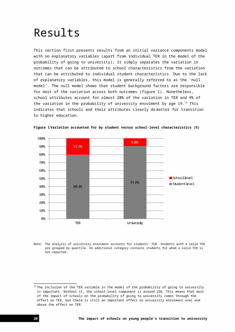
ResultsThis section first presents results from an initial variance components model with no explanatory variables (apart from individual TER in the model of the probability of going to university); it simply separates the variation in outcomes that can be attributed to school characteristics from the variation that can be attributed to individual student characteristics. Due to the lack of explanatory variables, this model is generally referred to as the ‘null model’. The null model shows that student background factors are responsible for most of the variation across both outcomes (figure 1). Nonetheless, school attributes account for almost 20% of the variation in TER and 9% of the variation in the probability of university enrolment by age 19.13 This indicates that schools and their attributes clearly do matter for transition to higher education.
Figure 1 Variation accounted for by student versus school-level characteristics (%)
Note: The analysis of university enrolment accounts for students’ TER. Students with a valid TER are grouped by quartile. An additional category contains students for whom a valid TER is not reported.
TERIt is well established that individual background characteristics such as gender, Indigenous status, length of in-country residence, socioeconomic status and academic achievement, as well as educational aspirations and perceptions of the school experience, strongly influence student outcomes (Considine & Zappala 2002; Khoo & Ainley 2005; Marjoribanks 2005; Marks 2010a; Rothman & McMillan 2003; Steering Committee for the Review of Government Service Provision 2009). Results from this analysis corroborate the importance of these student-level characteristics. Potential interactions between gender and other
13 The inclusion of the TER variable in the model of the probability of going to university is important. Without it, the school-level component is around 25%. This means that most of the impact of schools on the probability of going to university comes through the effect on TER, but there is still an important effect on university enrolment over and above the effect on TER.
NCVER 19
80.3%91.0%
19.7%9.0%
0%
10%
20%
30%
40%
50%
60%
70%
80%
90%
100%
TER University
School-level
Student-level
predictor variables were also investigated.14 No significant interactions were found, which meant there was no need to examine males and females separately.
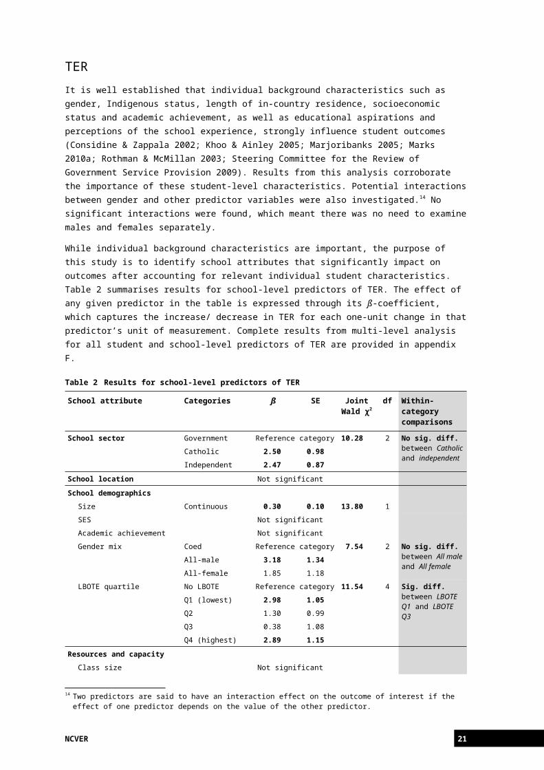
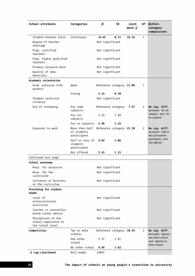
While individual background characteristics are important, the purpose of this study is to identify school attributes that significantly impact on outcomes after accounting for relevant individual student characteristics. Table 2 summarises results for school-level predictors of TER. The effect of any given predictor in the table is expressed through its ß-coefficient, which captures the increase/ decrease in TER for each one-unit change in that predictor’s unit of measurement. Complete results from multi-level analysis for all student and school-level predictors of TER are provided in appendix F.
Table 2 Results for school-level predictors of TER
School attribute Categories ß SE Joint Wald χ2
df Within-category comparisons
School sector Government Reference category 10.28 2 No sig. diff. between Catholic and independent
Catholic 2.50 0.98Independent 2.47 0.87
School location Not significant
School demographicsSize Continuous 0.30 0.10 13.80 1
SES Not significant
Academic achievement Not significant
Gender mix Coed Reference category 7.54 2 No sig. diff. between All male and All female
All-male 3.18 1.34All-female 1.85 1.18
LBOTE quartile No LBOTE Reference category 11.54 4 Sig. diff. between LBOTE Q1 and LBOTE Q3
Q1 (lowest) 2.98 1.05Q2 1.30 0.99
Q3 0.38 1.08
Q4 (highest) 2.89 1.15Resources and capacity
Class size Not significant
Student—teacher ratio Continuous -0.45 0.11 18.16 1
Degree of teacher shortage Not significant
Prop. certified teachers Not significant
Prop. highly qualified teachers Not significant
Primary resource base Not significant
Quality of educ. materials Not significant
Academic orientationAcad. pressure from parents Weak Reference category 11.09 1
Strong 2.33 0.70Student selection criteria Not significant
Use of streaming For some subjects Reference category 7.57 2 No sig. diff. between For all subjects and For no subjects
For all subjects 2.29 1.48
For no subjects 2.98 1.24
Exposure to work More than half of students participate
Reference category 21.10 2 No sig. diff. between Half or less of students participate and Not offered
Half or less of students participate
4.82 1.06
Not offered 3.43 1.15Continued next page
14 Two predictors are said to have an interaction effect on the outcome of interest if the effect of one predictor depends on the value of the other predictor.
20 The impact of schools on young people’s transition to university
School attribute Categories ß SE Joint Wald χ2
df Within-category comparisons
School autonomyResp. for resources Not significant
Resp. for the curriculum Not significant
Influence of business on the curriculum
Not significant
Providing for student needsLevel of extracurricular activities
Not significant
Teacher vs counsellor-based career advice
Not significant
Perceptions of the school experience at the school level
Not significant
Competition Two or more schools
Reference category 10.35 2 No sig. diff. between Against one other school and Against no other school
One other school 3.37 1.91
No other school 4.58 1.62
-2 Log-Likelihood Null model 32897
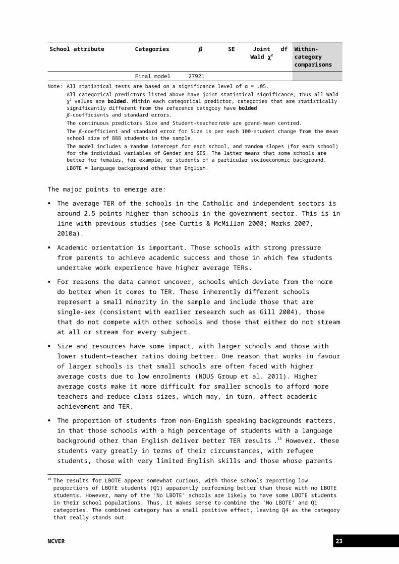
Final model 27921
Note: All statistical tests are based on a significance level of α = .05.All categorical predictors listed above have joint statistical significance, thus all Wald χ2 values are bolded. Within each categorical predictor, categories that are statistically significantly different from the reference category have bolded ß-coefficients and standard errors.The continuous predictors Size and Student-teacher ratio are grand-mean centred.The ß-coefficient and standard error for Size is per each 100-student change from the mean school size of 888 students in the sample.The model includes a random intercept for each school, and random slopes (for each school) for the individual variables of Gender and SES. The latter means that some schools are better for females, for example, or students of a particular socioeconomic background.LBOTE = language background other than English.
The major points to emerge are:
The average TER of the schools in the Catholic and independent sectors is around 2.5 points higher than schools in the government sector. This is in line with previous studies (see Curtis & McMillan 2008; Marks 2007, 2010a).
Academic orientation is important. Those schools with strong pressure from parents to achieve academic success and those in which few students undertake work experience have higher average TERs.
For reasons the data cannot uncover, schools which deviate from the norm do better when it comes to TER. These inherently different schools represent a small minority in the sample and include those that are single-sex (consistent with earlier research such as Gill 2004), those that do not compete with other schools and those that either do not stream at all or stream for every subject.
Size and resources have some impact, with larger schools and those with lower student—teacher ratios doing better. One reason that works in favour of larger schools is that small schools are often faced with higher average costs due to low enrolments (NOUS Group et al. 2011). Higher average costs make it more difficult for smaller schools to afford more teachers and reduce class sizes, which may, in turn, affect academic achievement and TER.
The proportion of students from non-English speaking backgrounds matters, in that those schools with a high percentage of students with a language background other
NCVER 21
than English deliver better TER results .15 However, these students vary greatly in terms of their circumstances, with refugee students, those with very limited English skills and those whose parents have low levels of secondary education usually facing much greater performance barriers (Australian Curriculum, Assessment and Reporting Authority 2011; NSW Department of Education and Communities 2011). Given the heterogeneity of the migrant student population, blanket statements about a ‘general’ positive effect from higher proportions of students with a language background other than English may be unsubstantiated.
Table 2 shows that a large number of school attributes were not statistically significant. Several potential explanations exist for why these attributes show no statistical significance. For some school variables based on aggregated student-level variables (e.g., academic achievement, perceptions of the school experience), it is likely that all the variation in outcomes is actually accounted for at the student level, and so there is no separate effect to be attributed to school atmospherics.
Some school-level variables, such as the proportions of certified and highly qualified teachers, have very little variation in the data from the outset. Given the international scope of PISA, these variables make sense for some countries, yet have limited relevance for Australia where almost all teachers are certified and qualified (see appendix A, table A2).
For other attributes, it is possible that they may be influenced or accounted for by other variables in the analysis. For example, higher levels of school autonomy have been associated with improved academic achievement outcomes (see OECD 2010). The fact that the present analysis revealed no significant effects for school autonomy might be due to such effects being absorbed by other variables. For instance, in those non-government schools with high levels of control over resources and the curriculum the impact of school autonomy variables might be absorbed by the variable sector.
Finally, the role of school-level socioeconomic status is particularly interesting. While both NAPLAN and PISA scores are affected by a school’s overall socioeconomic status (see Gonski et al. 2011; NOUS et al. 2011; OECD 2010; Perry & McConney 2010), results from the present study suggest that this is not the case for TER, after we have controlled for student characteristics including academic achievement at age 15. This finding is consistent with recent work by Marks (2010)16. It is important to emphasise that this result does not contradict the findings from prior research. These prior studies consider the impact of a school’s socioeconomic status on the entire student population during and towards the end of senior secondary schooling, whereas the present study examines the effect on TER at the end of senior secondary education conditioning on academic achievement at age 15. We also note that the sub-set of young people who self-select into obtaining a TER is inherently different from the general student population prior to senior secondary schooling.15 The results for LBOTE appear somewhat curious, with those schools reporting low proportions of LBOTE
students (Q1) apparently performing better than those with no LBOTE students. However, many of the ‘No LBOTE’ schools are likely to have some LBOTE students in their school populations. Thus, it makes sense to combine the ‘No LBOTE’ and Q1 categories. The combined category has a small positive effect, leaving Q4 as the category that really stands out.
16 In a previous study, Marks (2007) had also examined the impact of school attributes on Year 12 completion. His study found no evidence for a significant independent school-SES effect on Year 12 completion.
22 The impact of schools on young people’s transition to university
The multi-level model also includes variables that capture school idiosyncratic effects. These idiosyncratic effects refer to aspects of an individual school’s performance that can be identified statistically but which cannot be explained further using the LSAY data.17 As is shown in figure 2, the school characteristics included in the analysis explain seven percentage points of the 19.7% of variance which can be attributed to schools. Correspondingly, 12.7 percentage points of the variance are idiosyncratic school effects.18
Figure 2 Explained school-level variation for TER after multi-level modelling
The importance of idiosyncratic school effects is further illustrated by figure 3, which shows the distribution of these effects across schools. The difference between the school with the largest positive idiosyncratic effect and the school with the largest negative idiosyncratic effect is about 15 TER points (not considering outliers in the tail ends of the distribution). This means that these unexplained school effects have a sizeable impact on TER.
Figure 3 Distribution of school idiosyncratic effects on TER
17 As mentioned earlier, these effects contribute to a given school’s overall ‘ethos’, which has an important influence on individual student achievement (Hanushek et al. 2001).
18 Figure 2 also shows that the multi-level model explains more than half of the variation in TER that is attributable to student-level characteristics (that is, 41.6% explained student-level variation out of 80.3% total student-level variation).
NCVER 23
80.3%
38.7%
41.6%
19.7%12.7%
7.0%
0%
10%
20%
30%
40%
50%
60%
70%
80%
90%
100%
Null Model Final Model
Explained school variation
Unexplained school variation
Explained individual variation
Unexplained individual variation
24 The impact of schools on young people’s transition to university

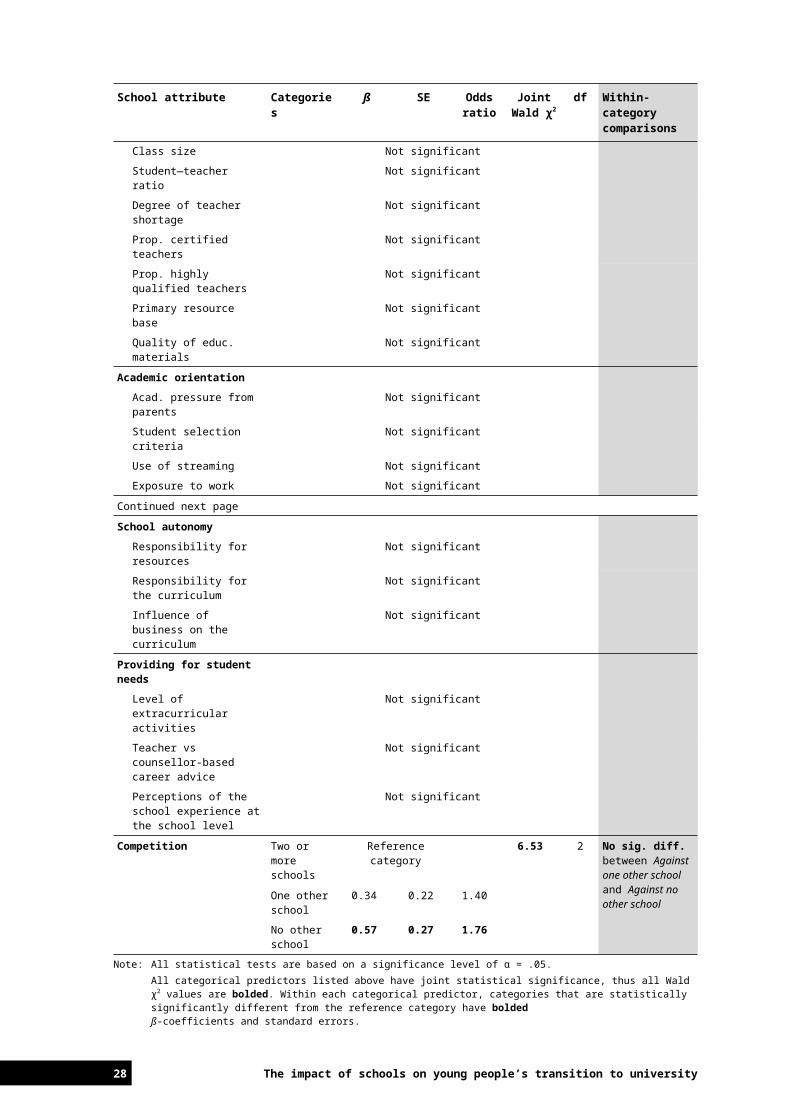
University enrolmentAbout half of the students in the sample had ‘ever commenced university’ by 2010 (modal age of 19). It is important to re-emphasise that the multi-level analysis for university enrolment accounts for individual TER. This means that school-level predictors showing statistical significance in table 3 are statistically significant with respect to university enrolment after controlling for the impact of individual TER and other relevant student factors. Complete results for all student and school-level predictors of university enrolment are provided in appendix F.
Table 3 Results for school-level predictors of university enrolment after accounting for TER
School attribute Categories ß SE Odds ratio19
Joint Wald χ2
df Within-category comparisons
School sector Government Reference Category 9.97 2 No sig. diff. between Catholic and independentCatholic 0.51 0.16 1.66
Independent 0.16 0.23 1.18
School location Not significant
School demographicsSize Not significant
SES Continuous 0.28 0.08 1.32 11.16 1
Academic achievement Not significant
Gender mix Not significant
LBOTE quartile No LBOTE Reference Category 42.93 4 Sig. diff. between LBOTE Q4 and each of LBOTE Q1, Q2 and Q3
Q1 (lowest) 0.25 0.23 1.28
Q2 0.46 0.16 1.58Q3 0.42 0.23 1.53
Q4 (highest) 1.12 0.17 3.06Resource and capacity
Class size Not significant
Student—teacher ratio Not significant
Degree of teacher shortage Not significant
Prop. certified teachers Not significant
Prop. highly qualified teachers
Not significant
Primary resource base Not significant
Quality of educ. materials Not significant
Academic orientationAcad. pressure from parents
Not significant
19 Readers are cautioned that the interpretation of results from multi-level models depends on the nature of the outcome variable. With continuous outcome variables such as TER, the ß-coefficients can be interpreted directly as the change in TER score points per every one-unit change in the predictor’s unit of measurement. For dichotomous outcome variables such as university enrolment, ß-coefficients cannot be interpreted directly and are therefore commonly converted to odds ratios. For instance, in the case of university enrolment the odds ratio for Catholic schools represents the odds of Catholic school students being enrolled in university study relative to the odds of students in government schools, who are chosen as the reference category. If the odds are equal for both Catholic and government school students, the odds ratio will be 1. If the odds of being enrolled in university are greater for students from Catholic schools, the odds ratio will be greater than 1. Likewise, if the odds are greater for students from government schools, the odds ratio will be less than 1. For continuous predictors such as school-level SES, the odds ratio is interpreted as the change in the odds of being enrolled in university as a result of a one-unit change in the predictors’ respective unit of measurement. For the standardised school-level SES variable, this means a change of one standard deviation.
NCVER 25
School attribute Categories ß SE Odds ratio
Joint Wald χ2
df Within-category comparisons
Student selection criteria Not significant
Use of streaming Not significant
Exposure to work Not significant
Continued next page
School autonomyResponsibility for resources Not significant
Responsibility for the curriculum
Not significant
Influence of business on the curriculum
Not significant
Providing for student needsLevel of extracurricular activities
Not significant
Teacher vs counsellor-based career advice
Not significant
Perceptions of the school experience at the school level
Not significant
Competition Two or more schools
Reference category 6.53 2 No sig. diff. between Against one other school and Against no other school
One other school
0.34 0.22 1.40
No other school
0.57 0.27 1.76
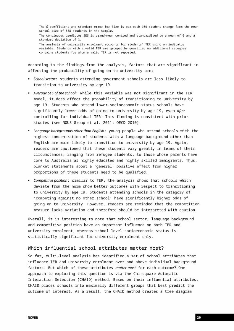
Note: All statistical tests are based on a significance level of α = .05.All categorical predictors listed above have joint statistical significance, thus all Wald χ2 values are bolded. Within each categorical predictor, categories that are statistically significantly different from the reference category have bolded ß-coefficients and standard errors.The ß-coefficient and standard error for Size is per each 100-student change from the mean school size of 888 students in the sample.The continuous predictor SES is grand-mean centred and standardised to a mean of 0 and a standard deviation of 1.The analysis of university enrolment accounts for students’ TER using an indicator variable. Students with a valid TER are grouped by quartile. An additional category contains students for whom a valid TER is not reported.
According to the findings from the analysis, factors that are significant in affecting the probability of going on to university are:
School sector: students attending government schools are less likely to transition to university by age 19.
Average SES of the school: while this variable was not significant in the TER model, it does affect the probability of transitioning to university by age 19. Students who attend lower-socioeconomic status schools have significantly lower odds of going to university by age 19, even after controlling for individual TER. This finding is consistent with prior studies (see NOUS Group et al. 2011; OECD 2010).
Language backgrounds other than English: young people who attend schools with the highest concentration of students with a language background other than English are more likely to transition to university by age 19. Again, readers are cautioned that these students vary greatly in terms of their circumstances, ranging from refugee students, to those whose parents have come to Australia as highly educated and highly skilled immigrants. Thus, blanket statements about a ‘general’ positive effect from higher proportions of these students need to be qualified.
Competitive position: similar to TER, the analysis shows that schools which deviate from the norm show better outcomes with respect to transitioning to university by age 19.
26 The impact of schools on young people’s transition to university
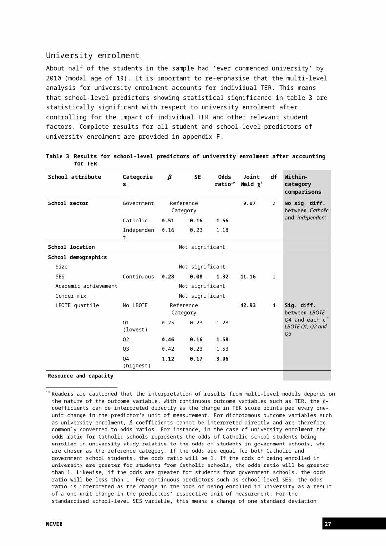
Students attending schools in the category of ‘competing against no other school’ have significantly higher odds of going on to university. However, readers are reminded that the competition measure lacks variation and therefore should be interpreted with caution.
Overall, it is interesting to note that school sector, language background and competitive position have an important influence on both TER and university enrolment, whereas school-level socioeconomic status is statistically significant for university enrolment only.
Which influential school attributes matter most?So far, multi-level analysis has identified a set of school attributes that influence TER and university enrolment over and above individual background factors. But which of these attributes matter most for each outcome? One approach to exploring this question is via the Chi-square Automatic Interaction Detection (CHAID) method. Based on their influential attributes, CHAID places schools into maximally different groups that best predict the outcome of interest. As a result, the CHAID method creates a tree diagram that allocates influential school attributes by order of relative importance.20 It is important to note that school attributes in the CHAID analyses for TER and university enrolment again represent net school effects, meaning that all influential student-level characteristics are accounted for.
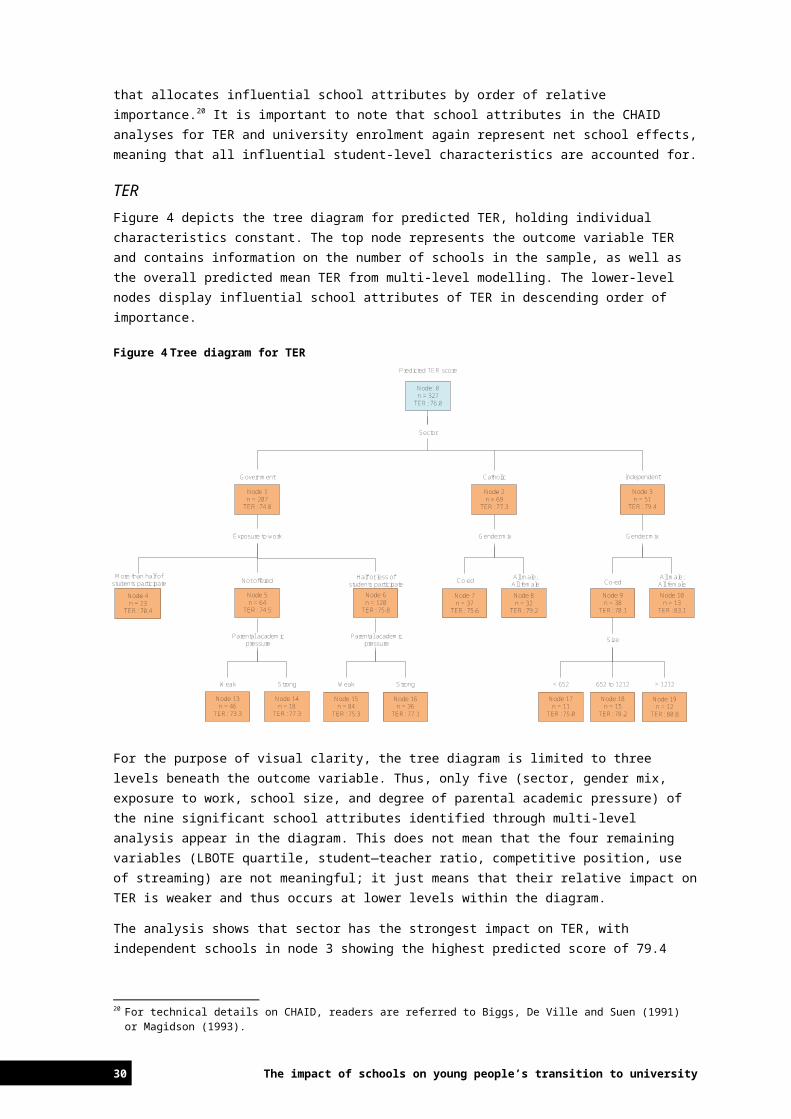
TERFigure 4 depicts the tree diagram for predicted TER, holding individual characteristics constant. The top node represents the outcome variable TER and contains information on the number of schools in the sample, as well as the overall predicted mean TER from multi-level modelling. The lower-level nodes display influential school attributes of TER in descending order of importance.
Figure 4 Tree diagram for TER
20 For technical details on CHAID, readers are referred to Biggs, De Ville and Suen (1991) or Magidson (1993).
NCVER 27
Node: 0n = 327
TER: 76.0
Node 1n = 207
TER: 74.8
Node 2n = 69
TER: 77.3
Node 3n = 51
TER: 79.4
Node 8n = 32
TER: 79.2
Node 7n = 37
TER: 75.6
Node 10n = 13
TER: 83.1
Node 9n = 38
TER: 78.1
Node 6n = 120
TER: 75.8
Node 5n = 64
TER: 74.5
Node 4n = 23
TER: 70.4
Node 13n = 46
TER: 73.3
Node 14n = 18
TER: 77.3
Node 15n = 84
TER: 75.3
Node 16n = 36
TER: 77.1
Node 19n = 12
TER: 80.8
Node 18n = 15
TER: 78.2
Node 17n = 11
TER: 75.0
Sector
Government Catholic Independent
More than half of students participate
Exposure to work
Not offered Half or less of students participate
Gender mix Gender mix
Co-ed All male;All female Co-ed
All male;All female
Size
< 652 652 to 1212 > 1212
Parental academic pressure
Weak Strong
Parental academic pressure
Weak Strong
Predicted TER score
For the purpose of visual clarity, the tree diagram is limited to three levels beneath the outcome variable. Thus, only five (sector, gender mix, exposure to work, school size, and degree of parental academic pressure) of the nine significant school attributes identified through multi-level analysis appear in the diagram. This does not mean that the four remaining variables (LBOTE quartile, student—teacher ratio, competitive position, use of streaming) are not meaningful; it just means that their relative impact on TER is weaker and thus occurs at lower levels within the diagram.
The analysis shows that sector has the strongest impact on TER, with independent schools in node 3 showing the highest predicted score of 79.4 points.21 For independent schools, gender mix is the next most important school attribute, whereby single-sex schools (node 10) outperform their coeducational counterparts (node 9).22 For coeducational independent schools, predicted TER further depends on school size. Nodes 17 to 19 illustrate that predicted TER improves as schools become larger within the independent sector. By comparison, the government sector experiences splits driven by academic orientation (either parental academic pressure on the school or the extent of work experience offered). Moreover, there is also considerable cross-over between different sectors. For instance, less vocationally oriented government schools that exhibit a high level of parental academic pressure perform as well as the coeducational Catholic schools and the smaller coeducational independent schools.
University enrolmentThe tree diagram in figure 5 illustrates the potential mechanism through which influential school attributes impact on the predicted probability of university enrolment, again controlling for individual TER, individual language background and other relevant individual characteristics. The average probability of university attendance across all schools in the sample is about 50% (node 0). This predicted probability is over 20% higher for schools with a high proportion of students with a language background other than English (node 3) when compared with the majority of schools that report having no such students (node 1).
Figure 5 Tree diagram for university enrolment
21 As shown in table 2, no practically meaningful difference in TER scores exists between independent and Catholic schools.
22 The effects of gender mix on government schools could not be reliably determined because only eight (3.7%) government schools in the TER sample were single-sex.
28 The impact of schools on young people’s transition to university
Node: 0n = 351
PROB: 0.51
Node 1n = 187
PROB: 0.44
Node 2n = 122
PROB: 0.58
Node 3n = 42
PROB: 0.65
Node 8n = 69
PROB: 0.63
Node 7n = 53
PROB: 0.51
Node 10n = 11
PROB: 0.74
Node 9n = 31
PROB: 0.62
Node 4n = 138
PROB: 0.40
Node 5n = 49
PROB: 0.53
LBOTE quartile
No LBOTE students LBOTE Q1 (lowest);LBOTE Q2; LBOTE Q3 LBOTE Q4 (highest)
Sector Sector Sector
Government Independent;Catholic Government Independent;
Catholic
School-level SES
GovernmentIndependent;
Catholic
Predicted probability of university enrolment
Node 13n = 30
PROB: 0.45
Node 12n = 62
PROB: 0.41
Node 11n = 46
PROB: 0.37
< -1.03 -1.03 to 0.06 > 0.06
Node 15n = 19
PROB: 0.55
Node 14n = 34
PROB: 0.49
School-level SES
< 0.06 > 0.06
Node 17n = 28
PROB: 0.60
Node 16n = 41
PROB: 0.65
LBOTE quartile
LBOTE Q2; LBOTE Q3
LBOTE Q1 (lowest)
Node 19n = 18
PROB: 0.66
Node 18n = 13
PROB: 0.58
School-level SES
< -0.67 > -0.67
Note: The analysis of university enrolment accounts for students’ TER using an indicator variable. Students with a valid TER are grouped by quartile. An additional category contains students for whom a valid TER is not reported.
Sector is again a critical factor, and the consistent role of school-level socioeconomic status across all government schools deserves attention.23 Government schools with average socioeconomic status and without students whose language background is other than English (node 13) show an 8% higher predicted probability of university enrolment than schools in the same category whose socioeconomic status is one standard deviation below the average (node 11). When comparing the latter group in node 11 with the group of non-government schools with a high proportion of students with a language background other than English (node 10), the difference in the predicted probability of university attendance is 37.3 percentage points. Again, however, blanket statements about a ‘general’ positive effect from higher proportions of these students need to be qualified, given the potentially complex interactions with other background factors, such as refugee status.
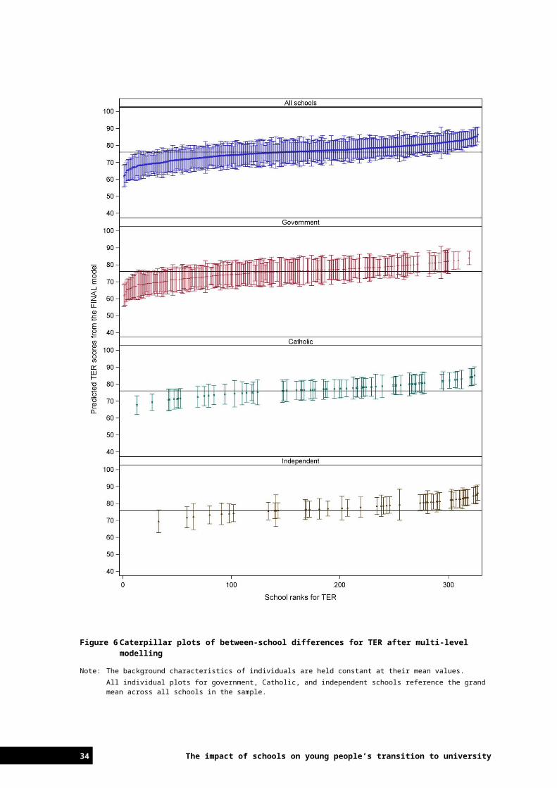
Further exploration of influential school attributesThis part of the analysis explores the distribution of school performance in more detail. The caterpillar plots in figures 6 and 7 rank each school by its predicted performance, where the predictions are based on the influential school attributes identified through multi-level modelling. To better assess the net school effect on each of the two outcomes, individual background variables are held constant at their mean values (that is, all students in the sample are ‘made’ to have the same average background characteristics).
A distinctive feature of the Australian school system is the significant proportion of students in the non-government sectors. To show the variation in school performance within and across sectors, caterpillar plots for each sector are provided below. Caterpillar plots can be interpreted as follows. For the TER outcome, the first caterpillar plot in figure 6 (‘all schools’)
23 Readers are reminded that the school-level socioeconomic status measure is standardised to a mean of 1 and a standard deviation of 0.
NCVER 29
shows how far the average TER of each individual school deviates from the average TER across all schools in the sample (that is, the grand mean). The grand mean TER of 76 points is represented by the horizontal zero line across the caterpillar plots. Each school in the plot features 95% confidence intervals, which capture the range of prediction error. The size of prediction error decreases as the number of students per school in the sample increases and vice versa. A school whose confidence interval does not cross the horizontal zero line has an average TER that is significantly different from the grand mean. The interpretation of the caterpillar plots for university enrolment in figure 7 follows the same logic, although here the horizontal zero line shows the grand mean probability of university enrolment of 51.3%.
The left and right tail ends of the caterpillar plot for ‘all schools’ in figure 6 show that a considerable number of schools perform above and below average with respect to TER. When examining the different sectors, government schools are more densely concentrated at the lower end of the TER scale, whereas Catholic and independent schools are better represented at the higher end.
The picture is similar with respect to university enrolment (figure 7), with the performance advantage of non-government schools becoming even more pronounced. However, several Catholic and independent schools do perform significantly below average.
30 The impact of schools on young people’s transition to university
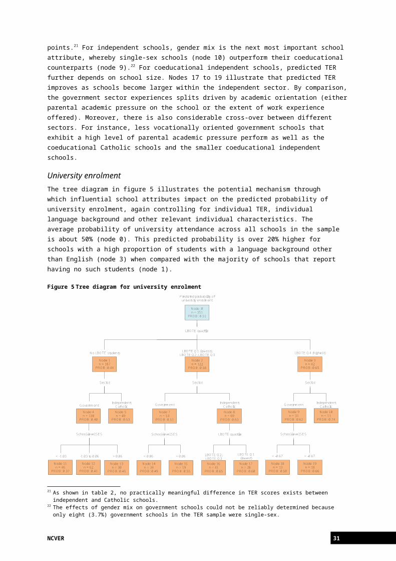
Figure 6 Caterpillar plots of between-school differences for TER after multi-level modelling
Note: The background characteristics of individuals are held constant at their mean values.All individual plots for government, Catholic, and independent schools reference the grand mean across all schools in the sample.
NCVER 31

Figure 7 Caterpillar plots of between-school differences for university enrolment after multi-level modelling
Note: The analysis of university enrolment accounts for students’ TER using an indicator variable. Students with a valid TER are grouped by quartile. An additional category contains students for whom a valid TER is not reported.The background characteristics of individuals are held constant at their mean values.All individual plots for government, Catholic, and independent schools reference the grand mean across all schools in the sample.
32 The impact of schools on young people’s transition to university

Comparing influential school attributes against performanceSo far the analysis has identified influential school attributes and assessed them in terms of their importance for TER and the probability of university enrolment by age 19. This final section of the analysis focuses on the highest and lowest performing schools to explore what distinctive characteristics each of these sets of school has. Two steps are taken to answer this question. The first step consists of undertaking a cluster analysis,24 which groups schools by their performance across both outcomes. Here, school performance is predicted from the multi-level model, assuming that each student has the characteristics of an ‘average’ student. The second step consists of identifying the actual characteristics of schools across performance clusters. Results from cluster analysis are shown in figure 8.
Figure 8 Cluster analysis of school performance
24 Cluster analysis is an exploratory data analysis method used to group similar entities across a range of variables. For more details on cluster analysis, readers are referred to Everitt et al. (2011). Detailed results of the cluster analysis are not presented due to space restrictions, but are available from the authors upon request.
NCVER 33
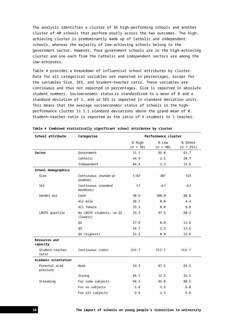
The analysis identifies a cluster of 36 high-performing schools and another cluster of 40 schools that perform poorly across the two outcomes. The high-achieving cluster is predominantly made up of Catholic and independent schools, whereas the majority of low-achieving schools belong to the government sector. However, four government schools are in the high-achieving cluster and one each from the Catholic and independent sectors are among the low-achievers.
Table 4 provides a breakdown of influential school attributes by cluster. Data for all categorical variables are reported in percentages, except for the variables Size, SES, and Student—teacher ratio. These variables are continuous and thus not reported in percentages. Size is reported in absolute student numbers. Socioeconomic status is standardised to a mean of 0 and a standard deviation of 1, and so SES is reported in standard deviation units. This means that the average socioeconomic status of schools in the high-performance cluster is 1.1 standard deviations above the grand mean of 0. Student—teacher ratio is reported as the ratio of X students to 1 teacher.
Table 4 Combined statistically significant school attributes by cluster
School attribute Categories Performance cluster% High(n = 36)
% Low(n = 40)
% Other(n = 251)
Sector Government 11.1 95.0 65.7
Catholic 44.4 2.5 20.7
Independent 44.4 2.5 13.6
School demographicsSize Continuous (number of students) 1,167 881 723
SES Continuous (standard deviations) 1.1 -0.7 -0.2
Gender mix Coed 30.6 100.0 88.8
All male 36.1 0.0 4.4
All female 33.3 0.0 6.8
LBOTE quartile No LBOTE students, or Q1 (lowest)
33.3 97.5 60.2
Q2 27.8 0.0 13.6
Q3 16.7 2.5 13.6
Q4 (highest) 22.2 0.0 12.8
Resources and capacityStudent–teacher ratio Continuous (ratio) 12.6 : 1 13.3 : 1 13.6 : 1
Academic orientationParental acad. pressure Weak 33.3 87.5 64.5
Strong 66.7 12.5 35.5
Streaming For some subjects 94.4 95.0 88.5
For no subjects 2.8 2.5 6.0
For all subjects 2.8 2.5 5.6
Exposure to work More than half of students participate
0.0 30.0 6.8
Half or less of students participate
38.9 37.5 58.6
Not offered 61.1 32.5 34.7
Competition Against two or more schools 83.3 82.5 84.5
Against one other school 11.1 10.0 6.4
Against no other school 5.6 7.5 9.2
34 The impact of schools on young people’s transition to university
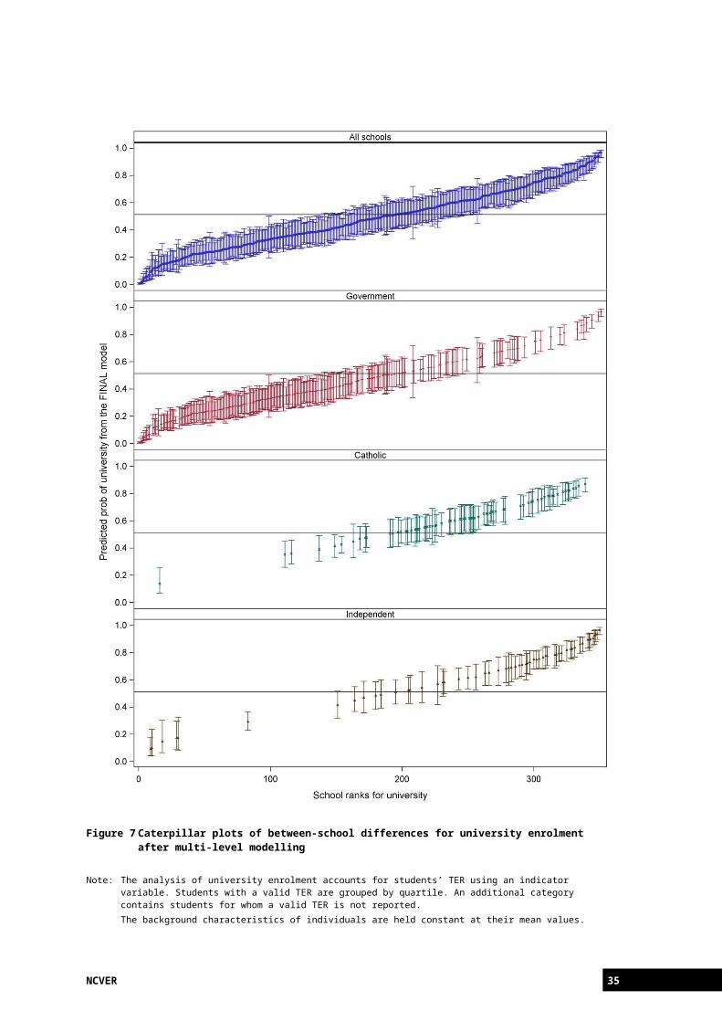
Table 4 shows that, when compared with low-performing schools, those in the high-performing cluster are larger, predominantly from the non-government sector, with much greater numbers of high-socioeconomic status students and students with a language background other than English and, in over two-thirds of all cases, single-sex. They are also those in which parental pressure for academic excellence is stronger and participation in work-related interventions is either modest or not offered. The table further indicates that streaming does not differentiate school performance: while 94.4% of the high-performing schools stream some subjects, around 95% of the low-performing schools also stream some subjects. Similarly, the Competition variable reveals little about what makes a high or low-performing school.
Other important variablesA number of variables were not statistically significant in the modelling, yet feature strongly in popular discussions about school systems. These variables relate to school selectivity, fees and regionality.
School selectivitySchool selectivity is captured by two variables in terms of academic selectivity and philosophical/religious selectivity (table 5). Selective schools are over-represented among high-performers, regardless of whether that selectivity is academic or philosophical/religious. However, selective schools do not dominate the cluster of high-performing schools. The fact that these variables are not significant in the multi-level models suggests that they have been subsumed by other variables, such as sector.
Table 5 Academic and instructional/religious selection criteria
School attribute Categories Performance cluster% High(n = 36)
% Low(n = 40)
% Other(n = 251)
Academic selectivity25 At least one criterion prerequisite 8.3 0.0 1.2
Considered 47.2 30.0 50.9
Not considered 44.4 70.0 48.0
Selectivity by instructional or religious philosophy26
At least one criterion prerequisite 29.4 2.5 13.0
Considered 38.3 5.0 30.3
Not considered 32.4 92.5 56.7
25 The index of academic selectivity (SELSCH) was derived from school principals’ responses on how much consideration was given to the following factors when students were admitted to the school, based on a scale from the response categories ‘not considered’, ‘considered’, ‘high priority’ and ‘prerequisite’ of items 19b and 19c in the school questionnaire: student’s record of academic performance (including placement tests); and recommendation of feeder schools. This index has the following four categories: (1) schools where neither of the two factors is considered for student admittance, (2) schools considering at least one of these two factors, (3) schools where at least one of these two factors is a high priority for student admittance, and (4) schools where at least one of these two factors is a prerequisite for student admittance. For statistical reasons, the categories ‘at least one of these two factors considered’ and ‘at least one of these two factors is high priority’ were combined.
26 This attribute is based on the same school principals’ responses on how much consideration was given to the following factors when students were admitted to the school. However, here the question is with regard to ‘parents’ endorsement of the instructional or religious philosophy of the school’ (item 19d of the school questionnaire).
NCVER 35
School feesWhile no direct measures of school income are available in the data, every school provides information on the proportion of funds coming from government, student fees and benefactors, as well as a residual category. Table 6 features funding sources by sector and cluster.
36 The impact of schools on young people’s transition to university
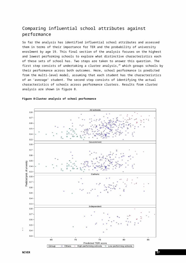
Table 6 Sources of funding by sector and cluster
Sector Funding Performance cluster% High(n = 36)
% Low(n = 40)
% Other(n = 251)
Government Government 78.8 84.3 80.6
Student fees 15.3 10.3 15.0
Benefactors 2.3 2.7 2.2
Other 3.5 2.7 2.3
Independent Government 23 60.0 48
Student fees 72.4 40.0 47.6
Benefactors 2.3 0 2.5
Other 2.3 0 2.0
Catholic Government 60.0 78.0 64.3
Student fees 36.1 19.0 30.4
Benefactors 2.2 0 1.4
Other 1.6 3.0 4.0
Student fees are higher on average in the high-performing schools, even among government schools. This pattern is particularly strong in the independent sector but also quite marked in the Catholic sector. Similarly, the low-performing cluster contains the highest proportion of primarily government-funded schools, irrespective of sector. Given that a higher share of funds from student fees has enabled non-government schools in particular to improve teaching quality by substantially lowering student—teacher ratios (Watson & Ryan 2010), it is likely that resources do play a role in assisting school performance.
School regionalitySome consideration also needs to be given to schools’ geographic location. Table 7 provides a geographic breakdown of schools by sector. Government schools have a much stronger presence in rural areas and small towns, whereas Catholic and independent schools are more prevalent in metropolitan areas.
Table 7 Geographic distribution of schools by sector
Location SectorGovernment
(%)Catholic
(%)Independent
(%)Rural (pop. size <3000) 13.1 2.7 1.7
Small town (pop. size 3000 to 15 000) 12.6 4.1 3.4
Town (pop. size 15 000 to 100 000) 23.9 24.7 20.3
City (pop. size 100 000 to 1 000 000) 23.4 37.0 28.8
Large city (pop. size >1 000 000) 27.0 31.5 45.8
Total 100 100 100
Table 8 lists schools’ geographic location by performance cluster. The table illustrates that low-performing schools gravitate more towards towns with a population of fewer than 100 000. It needs to be emphasised, however, that the absence of high-performing schools in smaller areas may be an artefact of the data and school sampling rather than a reflection of the actual geographic distribution on academic school quality. In other words, it is
NCVER 37
reasonable to expect that high-performing schools do operate in smaller areas as well, even though these schools may not have been captured in the data.
38 The impact of schools on young people’s transition to university
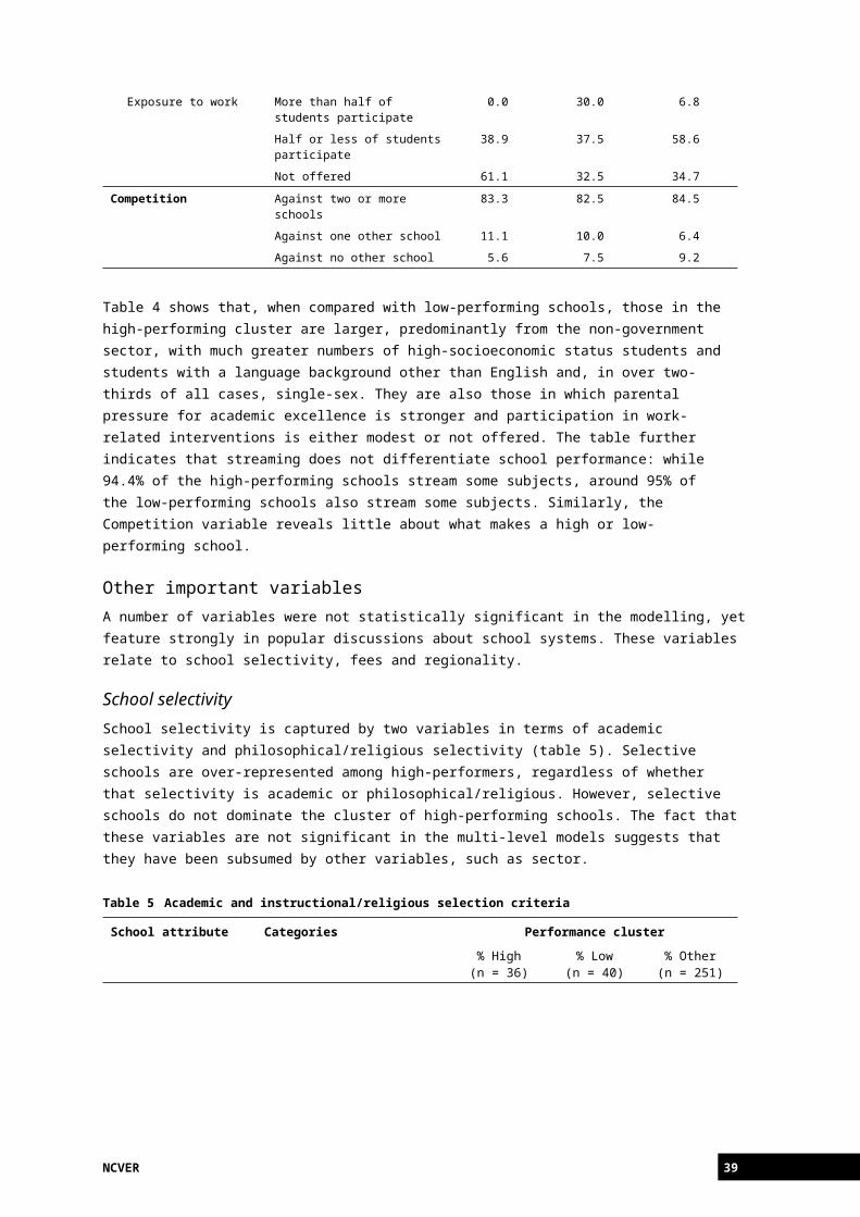
Table 8 Geographic distribution of schools by performance cluster
Location Performance cluster% High(n = 36)
% Low(n = 40)
% Other(n = 251)
Rural (pop. size <3000) - 22.5 7.2
Small town (pop. size 3000 to 15 000) - 25.0 7.6
Town (pop. size 15 000 to 100 000) - 27.5 25.9
City (pop. size 100 000 to 1 000 000) 33.3 12.5 28.3
Large city (pop. size >1 000 000) 66.7 12.5 31.1
Total 100 100 100
Differentiating the impact of schools by clusterAfter concentrating on the characteristics of high- and low-performing schools, this section considers the composition of individual school performance. Figure 9 categorises each school’s overall performance into four components: an overall intercept (of no interest because it is the same for all schools); the effect of measured school factors; the effect of measured student factors; and an idiosyncratic school component (that is, aspects of an individual school’s performance which can be identified statistically but cannot be explained further using the LSAY data27). In these graphs individual student characteristics are no longer held constant; instead, the focus here is on decomposing a given school’s raw average TER and probability of university enrolment.
Figure 9 presents each of these components in a school’s TER for the 36 high- and the 40 low-performing schools. In the high-performing cluster, the measured school attributes from the multi-level model make a sizeable contribution of between ten and 15 points to the overall TER. In many of the high-performing schools the strength of the school effect is thus on par with, or even exceeds, the strength of the individual student effect. Despite their small size, school idiosyncratic effects are interesting, in that they slightly decrease overall performance on TER for certain high-performing schools, although they increase performance for others.
Measured school effects have a much weaker impact on low-performing schools relative to the influence of individual student characteristics. For the lowest performing schools in the sample, measured and idiosyncratic school factors together have a negative effect on TER, even though for some schools the characteristics of individual students make a positive contribution.
27 As stated earlier, these idiosyncratic effects contribute to a given school’s overall ‘ethos’, which has an important influence on individual student achievement (Hanushek et al. 2001).
NCVER 39
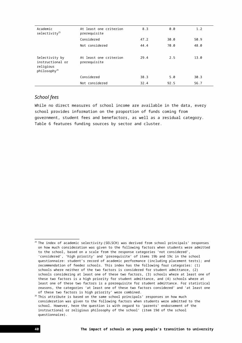
Figure 9 Components of total TER effect by cluster
Figure 10 shows results for the university enrolment outcome. As before, the binary nature of the university enrolment variable complicates the interpretation of results. For statistical reasons, the impact of the different school and student factors on university enrolment is expressed on a logistic scale on the X-axis of the two graphs. It is not possible to convert the impact of the individual components from a logistic to a probability scale, and so figure 10 needs to be interpreted visually.28
As with TER, schools generally have a positive impact on university enrolment in high-performing schools, with an increasingly negative impact as school performance diminishes. Overall, however, figure 10 demonstrates that young people’s individual characteristics play a much stronger role in relation to university enrolment than the characteristics of their schools, regardless of the performance cluster.
28 Additional information on the logistic scale is provided in appendix G.
40 The impact of schools on young people’s transition to university
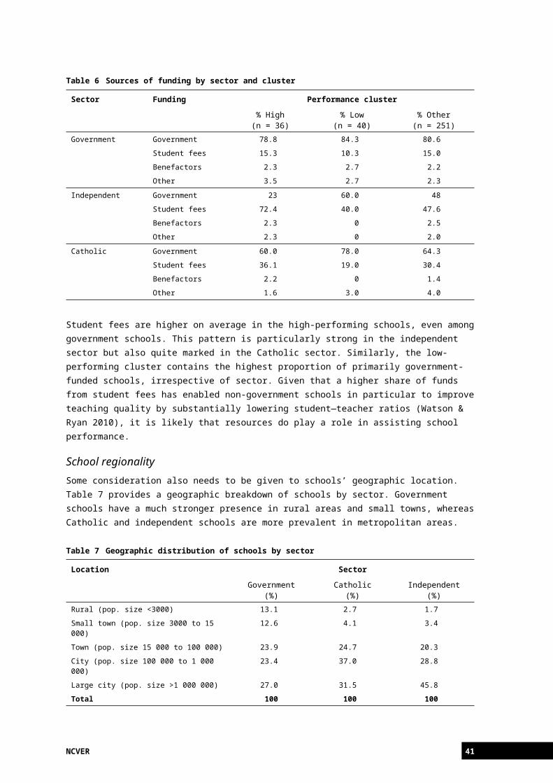
Figure 10 Components of total university enrolment effect by cluster
NCVER 41
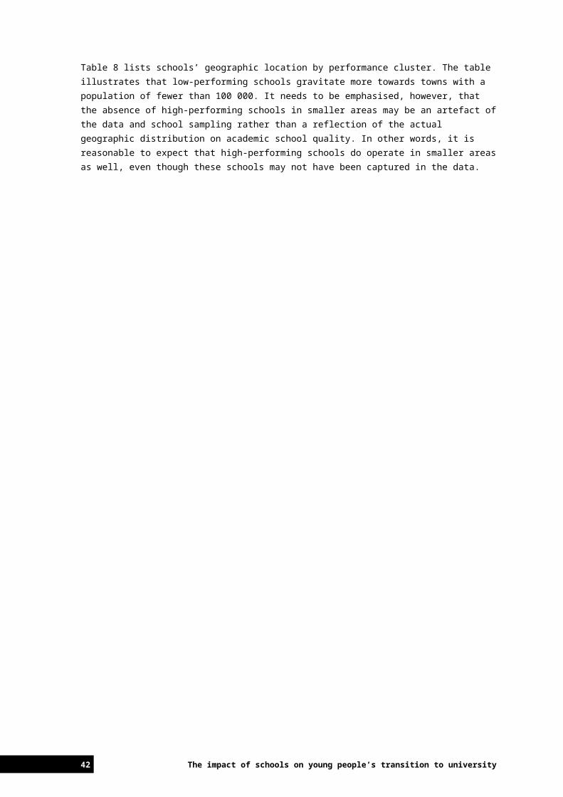
ConclusionThe purpose of this study was to determine whether, and to what extent, school characteristics can impact on TER and the probability of university enrolment by age 19. The analysis highlights the importance of a school’s characteristics. Although individual factors are the main drivers of success, school characteristics are responsible for almost 20% of the variation in TER and 9% of the variation in the probability of university enrolment, after controlling for TER. However, for TER only around seven percentage points of the variation can be attributed to the school characteristics that can be explained through the variables included in the analysis. The remaining 13 percentage points reflect features that are peculiar to certain schools, with these idiosyncratic (or school ‘ethos’) factors producing differences between schools that can be measured statistically but cannot be explained using the LSAY data.
The most influential factors to emerge from the analysis are the role of sector, academic orientation, differentiation from the norm and resourcing. In relation to sector, high-performing schools include government, Catholic and independent schools. However, even after controlling for relevant characteristics, the low-performing schools are almost all government. Academic orientation, as measured through parental pressure for the school to perform academically is important, as are the limitations imposed by the timetable of work-related programs. Schools that deviate from the norm (single-sex schools, the small number of schools that do not see themselves as competing with other schools, and the few which either stream all or no subjects) perform better than average, as do those with high proportions of students from language backgrounds other than English. The analysis further shows that resources do have some impact. On average, schools with lower student—teacher ratios obtain slightly better TERs, and student fees contribute more to school funds among schools in the high-performing cluster.
Another interesting insight this paper generates is with respect to the role of school-SES. Previous studies (Gonski et al. 2011; NOUS et al. 2011; OECD 2010; Perry & McConney 2010) find school-SES to affect academic achievement up to age 15. This study finds that a school’s overall socioeconomic status matters for university enrolment at age 19, but does not influence students’ TER outcomes at the end of senior secondary schooling, conditioning on academic achievement at age 15.
However, school SES does impact on the probability of going on to university for a given TER. Other school attributes which influence (positively) this probability are a high proportion of non-English speaking background students, and being Catholic and Independent rather than Government.
Overall, this analysis was about the important, albeit not exclusive, aim of schooling to prepare students for the transition to higher education. Results show that schools matter in relation to TER and the probability of going on to university over and above individual student characteristics.
42 The impact of schools on young people’s transition to university
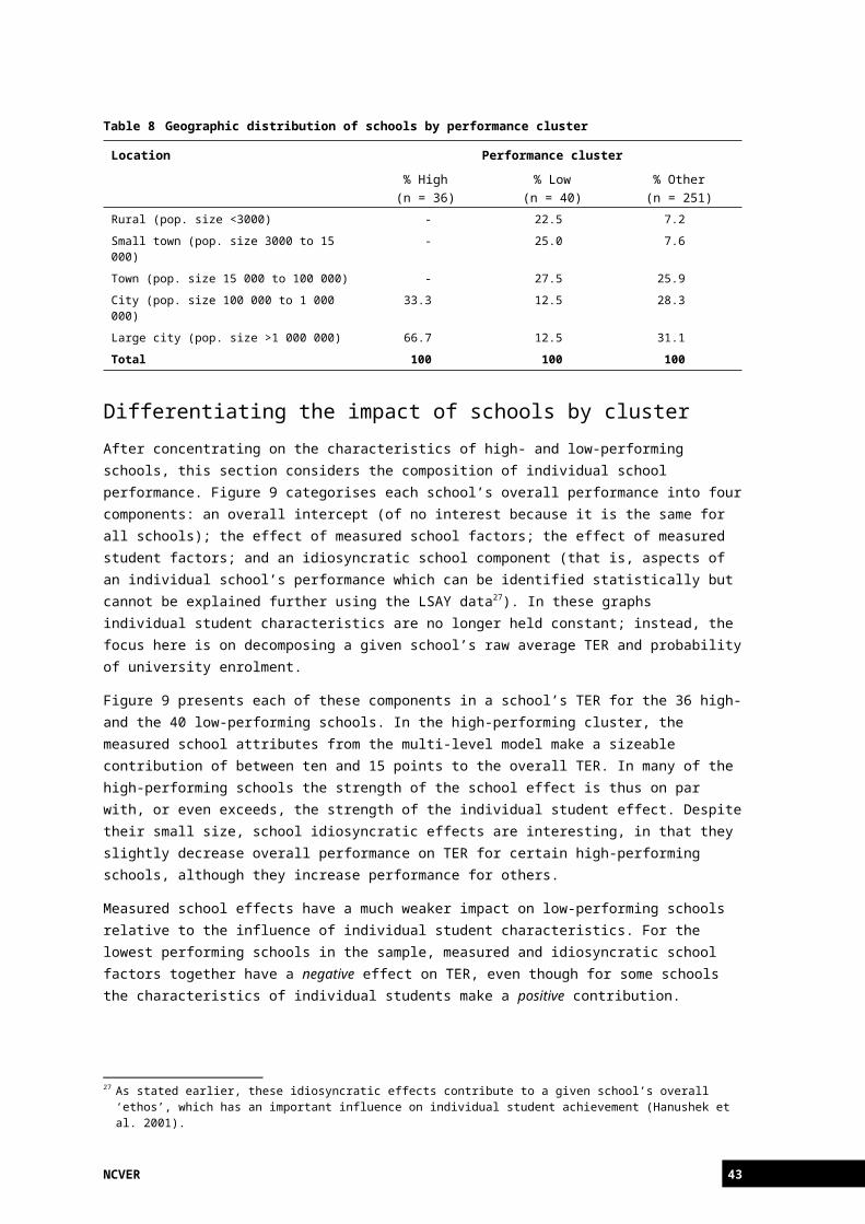
ReferencesAustralian Curriculum, Assessment and Reporting Authority 2011, Guide to understanding ICSEA,
ACARA, Sydney.Barrera, F, Fasih, T & Patrinos, HA 2009, Decentralized decision-making in schools: the theory
and evidence on school-based management, World Bank, Washington, DC.Biggs, D, De Ville, B & Suen, E 1991, ‘A method of choosing multiway partitions for classification
and decision trees’, Journal of Applied Statistics, vol.18, pp.49—62.Bruns, B, Filmer, D, & Patrinos, HA 2011, Making schools work: new evidence on accountability
reforms, World Bank, Washington, DC.Card, D, Dooley, MD & Payne, A 2010, ‘School competition and efficiency with publicly funded
Catholic schools’, American Economic Journal: Applied Economics, vol.2, pp.150—76.Considine, G & Zappala, G 2002, ‘The influence of social and economic disadvantage in the
academic performance of school students in Australia’, Journal of Sociology, vol.38, pp.129—48.
Curtis, DD & McMillan, J 2008, School non-completers: profiles and destinations, LSAY research report 54, ACER, Melbourne.
Everitt, B, Landau, S, Leese, M & Stahl, D 2011, Cluster analysis, 5th edn, Wiley & Sons, Chichester.
Fullarton, S 2002, Student engagement with school: individual and school-level influences, LSAY research report 27, ACER, Melbourne.
Fullarton, S, Walker, M, Ainley, J & Hillman, K 2003, Patterns of participation in Year 12, LSAY research report 33, ACER, Melbourne.
Gemici, S, Bednarz, A & Lim, P 2011, Getting tough on missing data: a boot camp for social science researchers, NCVER, Adelaide.
Gill, J 2004, Beyond the great divide: single-sex or co-education, University of New South Wales Press, Sydney.
Goldstein, H, Carpenter, J, Kenward, MG & Levin, KA 2009, ‘Multilevel models with multivariate mixed response types’, Statistical Modelling, vol.9, pp.173—97.
Gonski D, Boston, K, Greiner, K, Lawrence, C, Scales, B & Tannock, P 2011, Review of funding for schooling - final report, Canberra: DEEWR.
Hanushek, E, Kain, J, Markman, J & Rivkin, S 2001, Does peer ability affect student achievement?, National Bureau of Economic Research, Cambridge, MA.
Hattie, J 2009, Visible learning: a synthesis of over 800 meta-analyses relating to achievement, Routledge, New York.
Hedeker, D 2003, ‘A mixed effects multinomial logistic regression model’, Statistics in Medicine, vol.22, pp.1433—46.
Henderson, CR 1975, ‘Best linear unbiased estimation and prediction under a selection model’, Biometrics, vol.31, pp.423—47.
Homel, J & Ryan, C forthcoming, Aspirations and outcomes: size of the effect and the role of other factors, LSAY research report, NCVER, Adelaide.
Hox, JJ 2010, Multilevel analysis: techniques and applications, Routledge, New York.Khoo, ST & Ainley, J 2005, Attitudes, intentions and participation, LSAY research report 41, ACER,
Melbourne.Lamb, S 2007, ‘School reform and inequality in urban Australia: a case of residualising the poor’,
in Education and equity: international perspectives on theory and policy, eds R Teese & Lamb, Springer, Amsterdam.
Le, AT & Miller, PW 2002, Educational attainment in Australia: a cohort analysis, LSAY research report 25, ACER, Melbourne.
——2004, ‘High school graduation in Australia: do schools matter?’, Scottish Journal of Political Economy, vol.51, pp.194—208.
——2005, ‘Participation in higher education: equity and access’, Economic Record, vol.81, pp.152—65.Levin, B 2008, How to change 5000 schools: a practical and positive approach for leading
change at every level, Harvard Education Press, Cambridge, MA.
NCVER 43
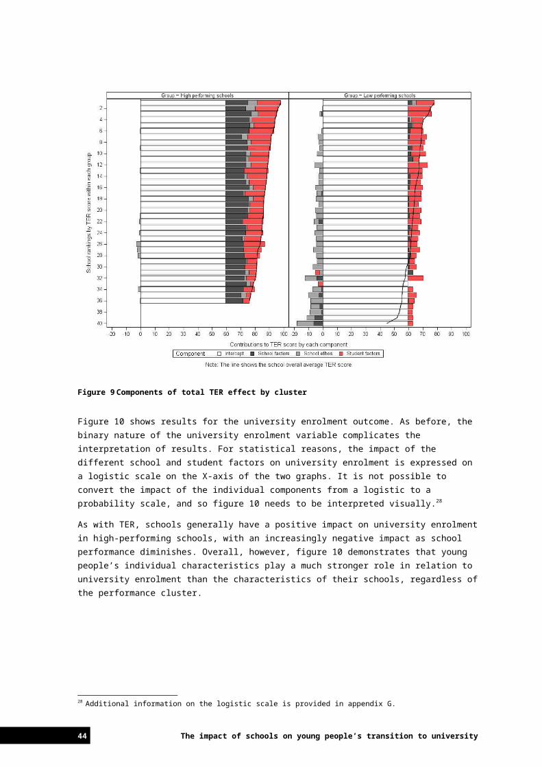
Lim, P 2011, Weighting the LSAY Program of International Student Assessment cohorts, NCVER, Adelaide.
Lim, P & Gemici, S 2011, Measuring the socioeconomic status of Australian youth, NCVER, Adelaide.
Lumsden, M & Stanwick, J 2012, Who takes a gap year and why? LSAY briefing paper 28, NCVER, Adelaide.
Magidson, J 1993, ‘The CHAID approach to segmentation modeling: Chi-squared automatic interaction detection’, in Handbook of marketing research, ed. R Bagozzi, Blackwell, London, pp.118—59.
Marjoribanks, K 2005, ‘Family background, adolescents’ educational aspirations, and Australian young adults’ educational attainment’, International Education Journal, vol.6, pp.104—12.
Marks, G 2007, ‘Do schools matter for early school leaving? Individual and school influences in Australia’, School Effectiveness and School Improvement, vol.18, pp.429—50.
——2010a, ‘What aspects of schooling are important? School effects on tertiary entrance performance’, School Effectiveness and School Improvement, vol.21, pp.267—87.
——2010b, ‘Socioeconomic and school sector inequalities in university entrance in Australia: the role of the stratified curriculum’, Educational Research and Evaluation, vol.16, pp.23—37.
Marks, G, McMillan, J & Hillman, K 2001, Tertiary entrance performance: the role of student background and school factors, LSAY research report 22, ACER, Melbourne.
McMillan, J & Marks, G 2003, School leavers in Australia: profiles and pathways, LSAY research report 31, ACER, Melbourne.
NSW Department of Education and Communities 2011, Discussion paper: Australian school funding arrangements, viewed 31 July 2012, <https://www.det.nsw.edu.au/media/downloads/about-us/news-at-det/announcements/discussion-paper.pdf>.
NOUS Group, Melbourne Graduate School of Education & National Institute for Labour Studies 2011, Schooling challenges and opportunities: a report for the review of funding for schooling panel, viewed 31 July 2012, <http://www.deewr.gov.au/Schooling/ReviewofFunding/Documents/Nous-SchoolingChallengesandOpportunities.pdf>.
OECD (Organisation for Economic Co-operation and Development) 2009, PISA 2006 technical report, viewed 31 July 2012, <http://www.pisa.oecd.org/dataoecd/0/47/42025182.pdf>.
——2010, PISA 2009 results: what makes a school successful? Resources, policies and practices, viewed 31 July 2012, <http://dx.doi.org/10.1787/9789264091559-en>.
Perry, L & McConney, A 2010, School socioeconomic composition and student outcomes in Australia: implications for educational policy, Australian Journal of Education, 54, 72–85.
Queensland Tertiary Admissions Centre 2011, 2010 Australian year 12 conversion table, viewed 31 July 2012, <http://www.qtac.edu.au/Applying-CurrentYr12/InterstateAdmissions.html>.
Rothman, S 2009, Estimating attrition bias in the Year 9 cohorts of the Longitudinal Surveys of Australian Youth, Technical report 48, ACER, Melbourne.
Rothman, S & McMillan, J 2003, Influences on achievement in literacy and numeracy, LSAY research report 36, ACER, Melbourne.
Steering Committee for the Review of Government Service Provision 2009, Overcoming Indigenous disadvantage: key indicators 2009, Productivity Commission, Canberra.
Twisk, JWR 2006, Applied multilevel analysis, Cambridge University Press, Cambridge.Watson, L & Ryan, C 2010, ‘Choosers and losers: the impact of government subsidies on
Australian secondary schools’, Australian Journal of Education, vol.54, pp.86—107.
44 The impact of schools on young people’s transition to university
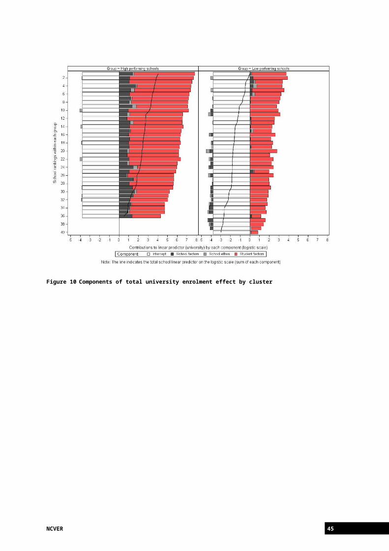
Appendix A: Descriptive statisticsTable A1Descriptive statistics for student-level predictors (unweighted)
Student attribute Categories TER(N = 3796)
University enrolment(N = 6315)
n % n %Student demographics
Gender Male 1697 44.7 3046 48.2
Female 2100 55.3 3269 51.8
Indigenous status Indigenous 91 2.4 278 4.4
Not Indigenous 3706 97.6 6037 95.6
Length of in-country residence Australian-born 2164 57.0 3786 60.0
First-generation 1239 32.6 1948 30.8
Foreign-born 355 9.3 492 7.8
Missing 39 1.0 89 1.4
Home language English 3416 90.0 5781 91.5
Not English 348 9.2 468 7.4
Missing 33 0.9 66 1.0
SES Continuous Mean: 0 SD: 1 Mean: 0 SD: 1
Acad. achievementAcad. achievement Continuous Mean: 0 SD: 1 Mean: 0 SD: 1
Year 12 completion Not completed Y12 - - 890 14.1
(only for university sample) Completed Y12 - - 5425 85.9
TER quartile No TER - - 2518 39.9
(only for university sample) TER Q1 (lowest) - - 982 15.6
TER Q2 - - 976 15.5
TER Q3 - - 891 14.1
TER Q4 (highest) - - 948 15.0
Aspirations and perceptionsYear 12 plans Not plan to complete 17 0.4 - -
(only for TER sample) Unsure about completing
60 1.6 - -
Plan to complete 3701 97.5 - -
Missing 19 0.5 - -
Educ. aspirations No tertiary study 154 4.1 464 7.3
Apprenticeship 103 2.7 577 9.1
University 3130 82.4 4023 63.7
Other 286 7.5 953 15.1
Missing 124 3.3 298 4.7
Perceptions of schooling Continuous Mean: 0 SD: 1 Mean: 0 SD: 1
Notes: The continuous predictors SES, Academic achievement, and Perceptions of schooling were standardised to a mean of 0 and a standard deviation of 1.Cases with missing data were excluded from the analysis. Even though multiple imputation is the recommended approach for handling missing data (see Gemici, Bednarz & Lim 2011), software that carries out multiple imputation procedures for multi-level models (as outlined in Goldstein et al. 2009) are currently still in an experimental stage. It was thus decided to not use such software in this analysis.
NCVER 45
Table A2Descriptive statistics for school-level predictors (unweighted)
School attribute Categories TER(N = 341)
University enrolment(N = 354)
n % n %School sector Government 214 62.8 222 62.7
Catholic 72 21.1 73 20.6
Independent 55 16.1 59 16.7
Location Not metropolitan 112 32.8 121 34.2
Metropolitan 229 67.2 233 65.8
School demographicsSize Continuous Mean: 888 SD: 397 Mean: 868 SD: 407
SES Continuous Mean: 0 SD: 1 Mean: 0 SD: 1
Acad. achievement Continuous Mean: 0 SD: 1 Mean: 0 SD: 1
Gender mix Co-ed 287 84.2 300 84.7
All male 25 7.3 25 7.1
All female 29 8.5 29 8.2
LBOTE quartile No LBOTE student 208 61.0 189 53.4
LBOTE Q1 (lowest) 24 7.0 36 10.2
LBOTE Q2 34 10.0 44 12.4
LBOTE Q3 38 11.1 43 12.1
LBOTE Q4 (highest) 37 10.9 42 11.9
Resources and capacityClass size Large (> 20) 310 90.9 315 89.0
Small (≤ 20) 26 7.6 34 9.6
Missing 5 1.5 5 1.4
Student-teacher ratio Continuous Mean: 13.5 SD: 2.6 Mean: 13.4 SD: 2.6
Degree of teacher shortage Continuous Mean: 0 SD: 1 Mean: 0 SD: 1
Prop. certified teachers Continuous Mean: 0.98 SD: 0.12 Mean: 0.98 SD: 0.13
Prop. highly qual. teachers Continuous Mean: 0.97 SD: 0.09 Mean: 0.97 SD: 0.09
Primary resource base Government 282 82.7 294 83.1
Non-government 46 13.5 46 13.0
Missing 13 3.8 14 4.0
Quality of educ. materials Continuous Mean: 0 SD: 1 Mean: 0 SD: 1
Academic orientationAcad. pressure from parents Weak 214 62.8 225 63.6
Strong 125 36.7 127 35.9
Missing 2 0.6 2 0.6
Student selection criteria At least one criterion prerequisite
11 3.2 11 3.1
Considered 237 69.5 243 68.6
Not considered 91 26.7 98 27.7
Missing 2 0.6 2 0.6
Use of streaming For some subjects 302 88.6 312 88.1
For no subjects 17 5.0 19 5.4
For all subjects 19 5.6 20 5.6
Missing 3 0.9 3 0.8
Exposure to work For more than half of students
30 8.8 36 10.2
For half or less of students
180 52.8 184 52.0
Not offered 125 36.7 127 35.9
Missing 6 1.8 7 2.0
Continued next page
46 The impact of schools on young people’s transition to university
School attribute Categories TER(N = 341)
University enrolment(N = 354)
n % n %
School autonomyResponsibility for resources Continuous Mean: 0 SD: 1 Mean: 0 SD: 1
Responsibility for curriculum Continuous Mean: 0 SD: 1 Mean: 0 SD: 1
Business influence on curriculum
No influence 54 15.8 55 15.5
Minor influence 254 74.5 262 74.0
Considerable influence
30 8.8 34 99.2
Missing 3 0.9 3 0.8
Providing for student needsLevel of extracurricular activities
Continuous Mean: 0 SD: 1 Mean: 0 SD: 1
Teacher vs counsellor-based career advice
Counsellor-based 129 37.8 131 37.0
Teacher-based 195 57.2 205 57.9
Missing 17 5.0 18 5.1
Perceptions of the school experience at the school level
Continuous Mean: 0 SD: 1 Mean: 0 SD: 1
CompetitionTwo or more schools 283 83.0 292 82.5
One other school 25 7.3 27 7.6
No other school 31 9.1 33 9.3
Missing 2 0.6 2 0.6
Notes: The continuous predictors School SES, School academic achievement, Teacher shortage, Quality of educational materials, Responsibility for resources, Responsibility for the curriculum, Extracurricular activities, and Perceptions of schooling are standardised to a mean of 0 and a standard deviation of 1.The continuous predictors School size and Student–teacher ratio report absolute numbers.The continuous predictors Proportion of LBOTE students, Proportion of properly certified students, and Proportion of highly qualified teachers report absolute proportions.Cases with missing data were excluded from the analysis. Even though multiple imputation is the recommended approach for handling missing data (see Gemici, Bednarz & Lim 2011), software for multiple imputation procedures in multi-level models (as outlined in Goldstein et al. 2009) is currently still in an experimental stage. It was thus decided to not use such software in this analysis.
Table A3Descriptive statistics for outcome variables (unweighted)
Outcome variable Categories TER(N = 3796)
University enrolment(N = 6315)
n % n %TER Continuous Mean: 77.14 SD: 16.41 - -
Ever commenced bachelor degree or higher by 2010
Yes - - 3039 48.1
No - - 3276 51.9
NCVER 47
Appendix B: Student-level measuresSocio-demographic factorsThe socio-demographic factors that impact on education and post-school transition outcomes in Australia are well understood. Key factors include gender, Indigenous status, length of in-country residence, language spoken at home, and socioeconomic status. On average, females and non-Indigenous students experience more successful educational outcomes than males or those from Indigenous backgrounds (Steering Committee for the Review of Government Service Provision 2009; McMillan & Marks 2003). Likewise, the academic achievement of foreign-born and first-generation students is higher when compared with students whose parents were born in Australia (Le & Miller 2004; Marks, McMillan & Hillman 2001). Finally, young people from socioeconomically disadvantaged strata fare worse with respect to school outcomes and participation in higher education (Considine & Zappala 2002; Fullarton et al. 2003; Le & Miller 2002, 2005; Marks, McMillan & Hillman 2001; NOUS Group et al. 2011).
For gender, Indigenous status, length of in-country residence and home language, the standard variables supplied in the LSAY—PISA dataset were used (see appendix A). To measure individual socioeconomic status, many LSAY-based studies use the Index of Economic, Social, and Cultural Status (ESCS), which is a standard variable available in the dataset. The ESCS index represents a mixture of parental occupation, parental education and home possessions to measure socioeconomic status across all 57 countries that participated in PISA 2006. The problem associated with ESCS is that the need for multi-country usability renders the measure less relevant in the Australian context. This point was addressed by creating a custom measure from PISA 2006 variables that is similar to ESCS, yet more accurately captures the variation in socioeconomic status of students and schools in Australia. Details on the creation of this measure are provided in appendix C as well as in Lim and Gemici (2011).
Academic achievementIndividual academic achievement is among the strongest determinants of educational success (Le & Miller 2002; Marks 2010a, 2010b). Individual academic achievement was determined by averaging students’ mathematics, reading, and science scores from PISA.29 Year 12 completion status and a TER indicator were also included in the model used to predict university enrolment status.
Educational aspirations and perceptions of schoolingYoung people’s post-school outcomes are strongly influenced by their aspirations towards attaining tertiary education qualifications and their cumulative perceptions of the school
29 Each student in PISA received a set of five achievement scores for mathematics, reading, and science, respectively. In this study, the first of five achievement scores was used from each subject area. Interested readers are referred to OECD (2009) for details on the creation of PISA achievement scores.
48 The impact of schools on young people’s transition to university
experience (Homel & Ryan forthcoming; Khoo & Ainley 2005; Marjoribanks 2005). Aspirations for tertiary education are measured in the 2006 base year on a five-point scale, ranging from no post-school study to completion of a university degree. Moreover, a measure of students’ intent to complete Year 12 was included in the analysis (for the TER outcome only).
Perceptions of the school experience are captured in the 2006 base year through a series of 30 individual items that were measured on a Likert-type scale, ranging from strongly agree to strongly disagree. A single measure capturing an individual’s perception of the school experience was created using a factor analysis procedure on the 30 individual items (see appendix D).
NCVER 49

Appendix C: Factor analysis for SES measureA custom measure of socioeconomic status was created by factor-analysing 21 items from the PISA 2006 student questionnaire. The 21 items captured proxies for income/wealth, cultural resources, and educational resources. The results from factor analysis are presented below. Readers are further referred to Lim and Gemici (2011) for a detailed description on the motivation and methodology for deriving the custom socioeconomic status measure.
Table C1Eigenvalues for SES factor analysis
Variable Value Prop. variance explained
Cumulative
1 5.979 0.285 0.285
2 2.933 0.140 0.424
3 1.575 0.075 0.499
4 1.256 0.060 0.559
5 1.144 0.054 0.614
6 0.968 0.046 0.660
7 0.945 0.045 0.705
8 0.771 0.037 0.741
9 0.702 0.033 0.775
10 0.632 0.030 0.805
11 0.606 0.029 0.834
12 0.533 0.025 0.859
13 0.526 0.025 0.884
14 0.459 0.022 0.906
15 0.445 0.021 0.927
16 0.416 0.020 0.947
17 0.351 0.017 0.964
18 0.303 0.014 0.978
19 0.275 0.013 0.991
20 0.200 0.010 1.001
21 -0.019 -0.001 1.000
50 The impact of schools on young people’s transition to university
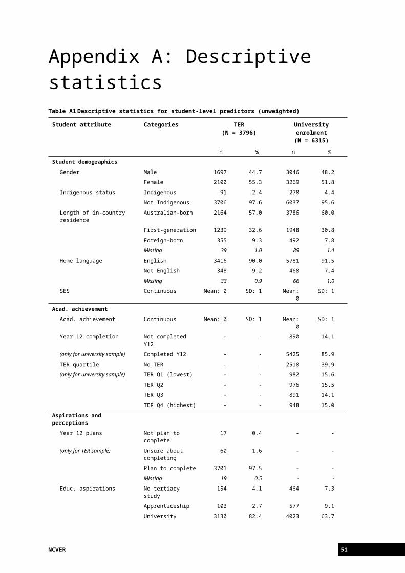
Figure C1 Scree plot from SES factor analysis
Table C2One-factor model for SES measure
Variable Socioeconomic status (Factor 1)
Desk 0.652
Room 0.287
Place to study 0.555
Educ. software 0.569
Internet 0.669
Calculator 0.559
Literature 0.715
Poetry 0.677
Art 0.507
Reference books 0.620
Dictionary 0.754
Dishwasher 0.453
DVD/VCR 0.586
Pay TV 0.122
Digital TV 0.500
Plasma TV 0.233
No. of mobile phones 0.408
No. of televisions 0.159
No. of computers 0.503
No. of cars 0.272
No. of books 0.485
NCVER 51
0.000
1.000
2.000
3.000
4.000
5.000
6.000
7.000
0 5 10 15 20 25
Eige
nval
ue
Component number
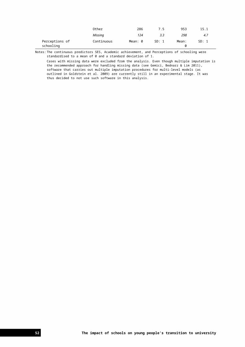
Appendix D: Factor analysis for perceptions of schooling measureA single measure capturing student perceptions of the school experience was created by factor-analysing items ST46N01—ST46N30 from the PISA 2006 student questionnaire. Items were measured on a four-level Likert-type scale ranging from strongly agree (1) to strongly disagree (4). For use in multi-level modelling, the final factor scores were multiplied by (-1) to convert them into a positive scale (that is, higher values indicate more positive perceptions). Results from factor analysis for the 30 items are presented below.
Table D1Eigenvalues for perceptions of schooling factor analysis
Variable Value Prop. variance explained
Cumulative
1 12.241 40.805 40.805
2 1.863 6.210 47.015
3 1.557 5.191 52.206
4 1.231 4.104 56.311
5 1.028 3.428 59.740
6 0.882 2.941 62.681
7 0.798 2.662 65.343
8 0.752 2.509 67.853
9 0.683 2.278 70.131
10 0.635 2.119 72.250
11 0.588 1.961 74.211
12 0.584 1.946 76.158
13 0.529 1.764 77.923
14 0.511 1.704 79.627
15 0.504 1.680 81.308
16 0.490 1.635 82.943
17 0.460 1.534 84.478
18 0.442 1.475 85.954
19 0.423 1.411 87.365
20 0.413 1.377 88.743
21 0.396 1.320 90.063
22 0.382 1.273 91.337
23 0.381 1.272 92.609
24 0.364 1.213 93.823
25 0.348 1.160 94.983
26 0.331 1.104 96.088
27 0.315 1.052 97.140
28 0.294 0.980 98.121
29 0.284 0.948 99.069
30 0.279 0.930 100.000
52 The impact of schools on young people’s transition to university
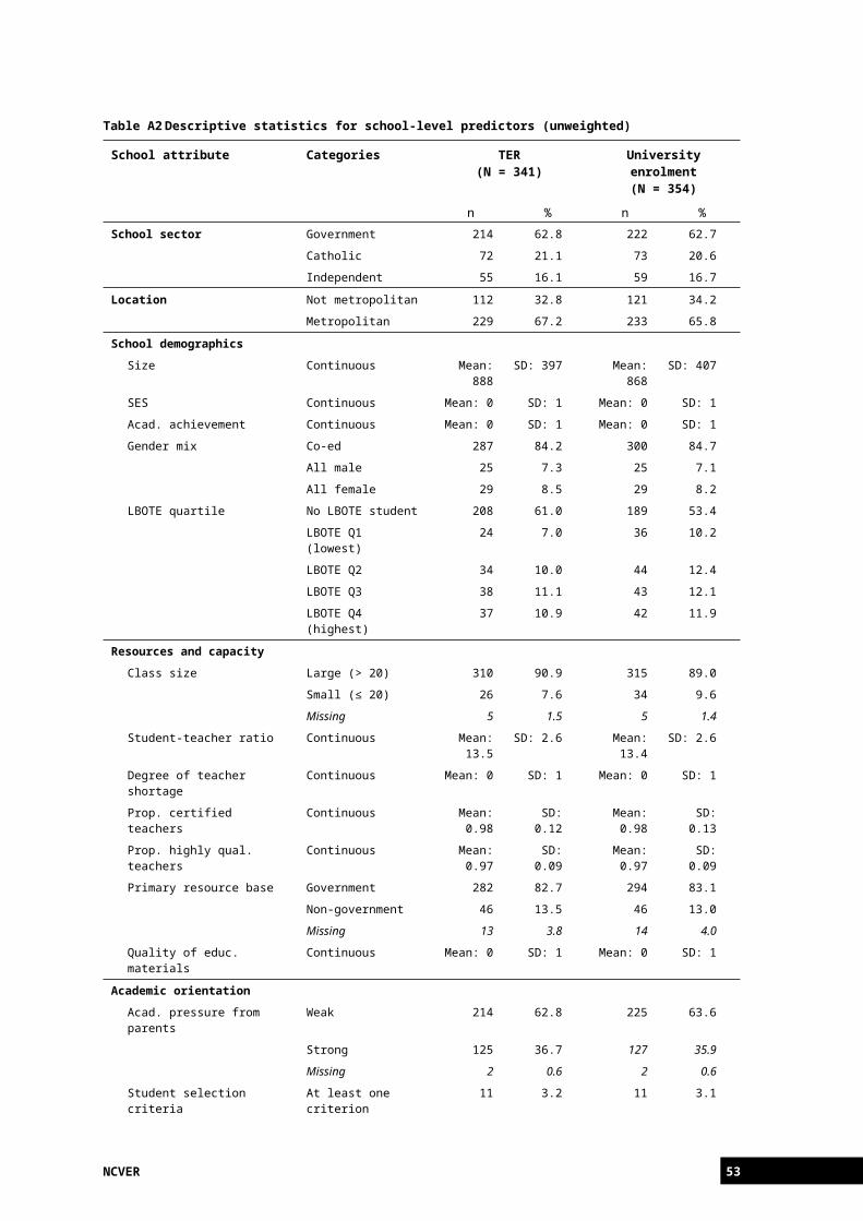
Figure D1 Scree plot from perceptions of schooling factor analysis
Table D2One-factor model for perceptions of schooling measure
Variable Perceptions of schooling (Factor 1)
School work is interesting 0.642
Teachers are fair and just 0.548
Things I learn are important 0.679
I learnt to work hard 0.663
I feel happy 0.660
Teachers listen to what I say 0.652
I achieved satisfactory standard in my work 0.605
I like learning 0.702
I get enjoyment from being here 0.658
School work is good preparation for the future 0.681
I like to ask questions in class 0.541
Teachers give me marks I deserve 0.621
I’ve acquired skills that will be useful 0.682
I always achieve a satisfactory standard in my school work 0.604
I like to do extra work 0.559
Teachers take personal interest 0.608
I really like to go to school each day 0.642
I enjoy what I do 0.698
I always try to do my best 0.590
Things I learn will help me in adult life 0.642
I know how to cope with school work 0.600
Teachers help me do my best 0.684
I get excited about school work that we do 0.624
I find learning a lot of fun 0.640
I’m given the chance to do interesting work 0.644
I know I can do well to be successful 0.619
Things taught are worth learning 0.699
I feel safe and secure 0.621
Teachers treat me fairly in class 0.669
NCVER 53
0
2
4
6
8
10
12
14
0 5 10 15 20 25 30 35
Eige
nval
ue
Component number
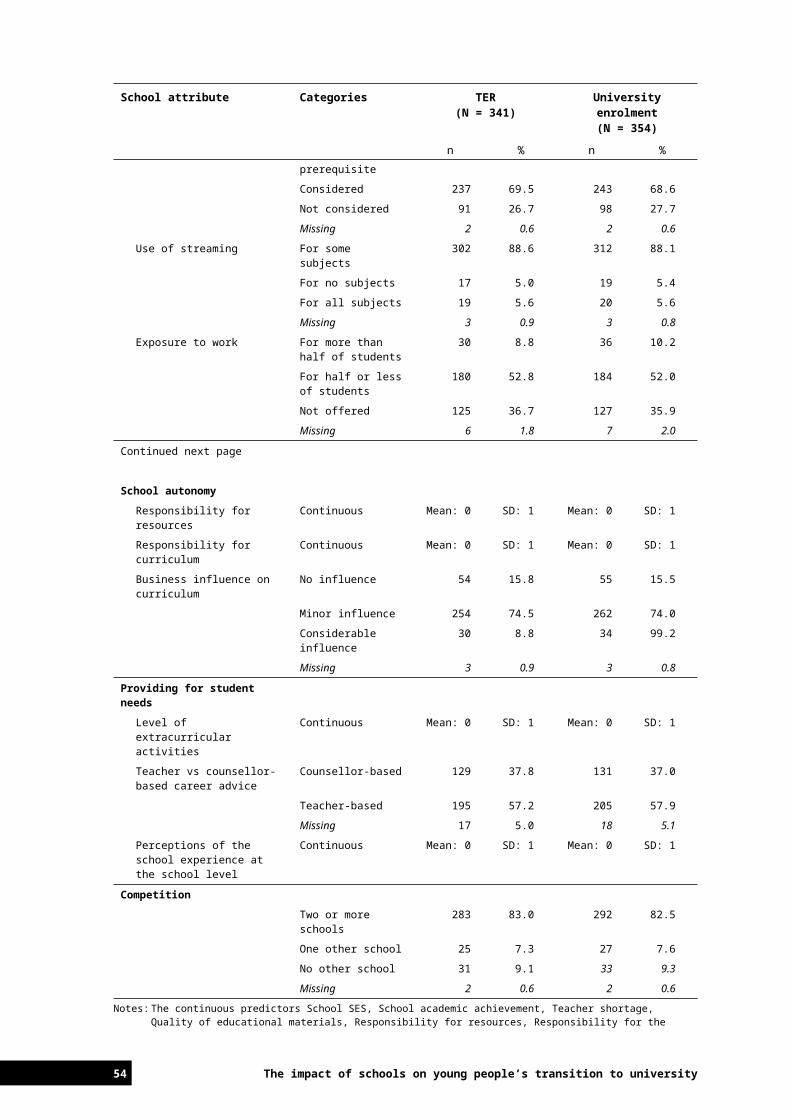
I have success as a student 0.629
54 The impact of schools on young people’s transition to university
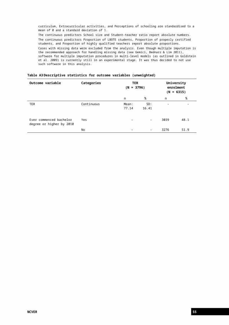
Appendix E: Technical details on multi-level modellingThe general multi-level model fitted in this analysis can be written as
Y ij=β0 j+β1 j X1 j+r ijβ0 j=γ 00+u0 jβ1 j=γ 10+u1 j
where rij N (0 , σ st2 ), and σ st2 is the student level variance and u0 jand u1 jare the variance
components for school intercepts and school slopes respectively, such that
(u0 ju1 j) N [(00), (σ00 σ01σ10 σ11)],
where σ 00 represents the variability in school intercepts, σ 11 is the variability in slopes and σ 01 is the covariance between intercepts and slopes.
In the mixed-model framework, this model is written as
Y ij=[ γ00+γ 10 X1 j ]+(u¿¿0 j+u1 j X1 j+rij )¿
where the terms in [ ] represent fixed effects and those in ( ) represent random effects. The fixed effects are fitted and tested first and only random effects included are u0 j, and rij, that is, the random school and individual level variances. The final tests conducted are those that fit the random effects for the individual level characteristics (u1 j X1 j).
Different strategies exist for adding student and school-level predictor variables to build a multi-level model (Hox 2010; Twisk 2006). In this study, random-intercept models were fitted for each outcome that contained all student and school-level predictors as fixed effects. Using Wald tests, non-significant predictors were successively eliminated from the models. Finally, statistically significant random coefficients for student-level predictors were included (using changes in log-likelihoods). The final model for each respective outcome contained all statistically significant fixed and random effects at the student level, as well as all statistically significant fixed effects at the school level.
The interpretation of the coefficients resulting from a multi-level model is the same as for ordinary regression. However, given that schools are fitted as random effects the predicted means or probabilities for schools are based on Best Linear Unbiased Prediction (BLUP; Henderson 1975).
Appropriate student- and school-level weights were applied to all multi-level analyses. Cases with missing data were excluded. Even though multiple imputation is the recommended approach for handling missing data (see Gemici, Bednarz & Lim 2011), software for multiple imputation procedures in multi-level models (as outlined in Goldstein et al. 2009) is currently still in an experimental stage. Therefore, it was decided to not use multiple imputation in the context of this multi-level modelling study.
The intra-class correlation (ICC) captures the extent to which individuals within a school are similar to each other. In particular, the ICC provides a mechanism for determining how
NCVER 55
much of the total variation in a particular outcome can be attributed to each level included (that is, students, school) in the multi-level model. High values of the ICC indicate that schools play an important part in explaining the variation in the given outcome. Small values indicate that student background characteristics play a larger part in explaining the relationship with the outcome of interest.
In this paper, the ICC for the continuous TER outcome yields the percentage of total variation attributable to schools and individuals. For the binary university enrolment
outcome, the error variance is constant at π2
3 (Hedeker 2003) and the ICC does not provide
the same information. For this model, the change in actual variance components is a more appropriate measure of variance explained (see appendix F, table F1).
56 The impact of schools on young people’s transition to university
Appendix F: Results from multi-level modellingTable F1 provides the variance components from the initial null model and the final model for each outcome. The null model is the basic variance components model with a random intercept but without any predictors. The final model is the model with all statistically significant student and school-level predictors for each respective outcome. σ2school shows the unexplained variance in school intercepts. σ2gender and σ2ses are variance components for the amount of variation explained by student gender and student socioeconomic status in schools (that is, they represent variation at the individual level). σ2e is the unexplained variation between students in schools. Note that for university enrolment σ2gender and σ2ses were not statistically significant random effects.
Table F1 Variance components for null and final models across outcomes
TER UniversityVar. comp. Null model Final model Null model Final modelσ2
school 57.34 20.36 1.08 0.06
σ2gender 3.11
σ2ses 28.21
σ2e 233.05 143.56
Total 290.39 195.24 4.37 3.35
The variance component for schools (σ2school) has decreased substantially in the final models when compared with the null models for each respective outcome. For the TER outcome, the reduction in the variance component for schools (σ2school ) must be considered in conjunction with the reduction in error variance (σ2e) because the multi-level model explains both school and student-level variance. As the models include more predictor variables, the total variation present in TER is reduced. A logistic model is used for the university enrolment outcomes, so the error variance remains constant at π 2
3 (Hedeker 2003).
Tables F2—F7 provide detailed results from the multi-level modelling for TER and the probability of university enrolment at age 19. The following applies to these tables:
All statistical tests were based on a significance level of α = 0.05.
All continuous predictors are grand-mean-centred.
The reference category for categorical predictors is marked as [R].
For categorical predictors, Wald χ2 statistics indicate the joint value.
The final model shows only statistically significant predictors, so all Wald χ2 values are bolded. For categorical predictors, those categories that are statistically significantly different from the reference category have bolded beta coefficients and standard errors.
NCVER 57
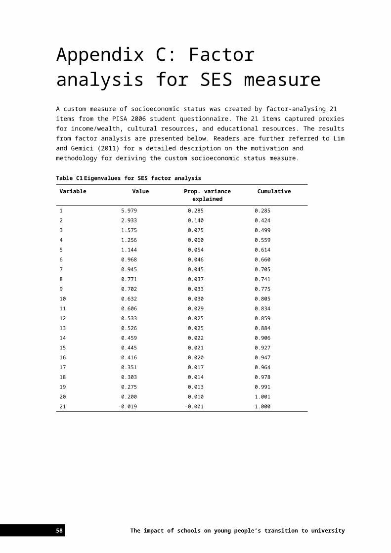
Table F2 Results for student-level predictors of TER
Student attribute Categories df Joint Wald χ2 Model 3 (Final model, n = 3388)
Model 1 Model 2 Wald χ2 Coeff. SEStudent demographics
Gender Male [R] 1 15.73 18.49 9.05Female 3.731 0.879
Indigenous status
Indigenous [R] 1 4.25 4.21 5.26
Not indigenous 5.084 2.217Length of in-country residence
Australian-born [R] 2 4.55 10.23 10.53
First-generation 1.475 0.624Foreign-born 3.091 1.009
Home language
English [R] 1 2.85 d
Not English
SES Continuous 1 3.78 6.49 6.66 0.779 0.302Academic achievement
Acad. achievement
Continuous 1 288.85 504.29 549.41 7.111 0.303
Aspirations and perceptions
Y12 plans Not plan to complete [R]
2 0.43 d
Unsure about completing
Plan to complete
Educ. aspirations
No tertiary study [R] 3 41.17 42.32 41.20
Apprenticeship 1.333 2.269
University 5.312 1.856Other -1.043 2.012
Perceptions of schooling
Continuous 1 28.91 44.73 43.43 2.374 0.36
Note: In model 3, the student-level predictors Gender and SES were fitted as random effects.
58 The impact of schools on young people’s transition to university
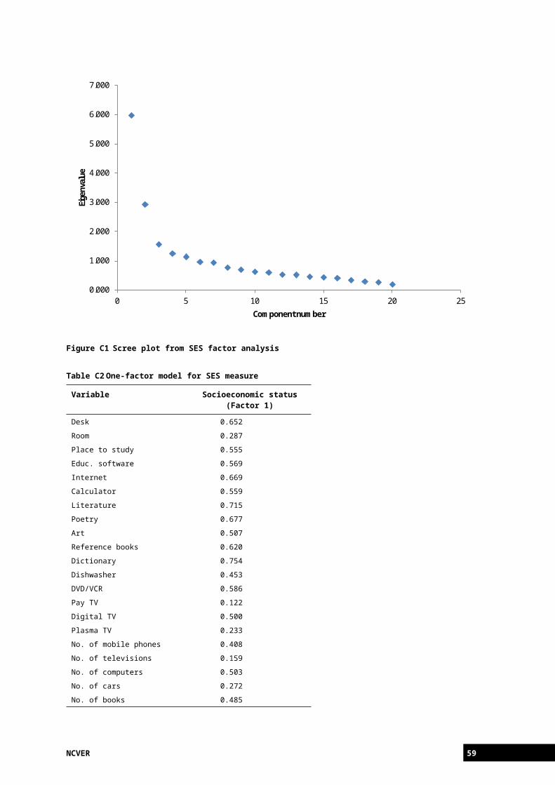
Table F3 Results for school-level predictors of TER
School attribute Categories df Joint Wald χ2 Model 3 (Final model, n = 329)
Model 1 Model 2 Wald χ2 Coeff. SE
School sector Government [R] 2 10.11 10.35 10.28Catholic 2.501 0.976Independent 2.472 0.869
School location Not metropolitan [R] 1 1.19 dMetropolitan
School demographics
Size Continuous 1 12.04 13.49 13.80 0.003 0.001SES Continuous 1 0.22 dAcad. achievement
Continuous 1 3.66 d
Gender mix Co-ed [R] 2 5.65 9.53 7.54All male 3.176 1.342All female 1.852 1.18
LBOTE quartile No LBOTE students 4 11.77 8.65 11.54LBOTE Q1 (lowest) 2.977 1.046LBOTE Q2 1.301 0.993LBOTE Q3 0.384 1.078LBOTE Q4 (highest) 2.886 1.154
Resources and capacity
Class size Large (> 20) [R] 1 1.15 dSmall (≤ 20)
Student–teacher ratio
Continuous 1 9.98 16.20 18.16 -0.447 0.105
Degree of teacher shortage
Continuous 1 2.79 d
Prop. certified teachers
Continuous 1 2.55 d
Prop. highly qual. teachers
Continuous 1 2.78 d
Primary resource base
Government [R] 1 0.20 d
Non-governmentQuality of educ. materials
Continuous 1 0.02 d
Academic orientation
Acad. press. from parents
Weak [R] 1 5.96 10.65 11.09
Strong 2.328 0.699Student selection criteria
At least one prereq. [R]
2 1.08 d
ConsideredNot considered
Use of streaming For some subjects [R]
2 12.35 7.02 7.57
For no subjects 2.984 1.24For all subjects 2.292 1.48
Exposure to work
For more than half of students [R]
2 15.53 25.68 21.10
For half or less of students
4.817 1.058
Not offered 3.426 1.153
NCVER 59

School attribute Categories df Joint Wald χ2 Model 3 (Final model, n = 329)
Model 1 Model 2 Wald χ2 Coeff. SE
Continued next page
School autonomyResp. for resources
Continuous 1 1.38 d
Resp. for curriculum
Continuous 1 0.29 d
Business influence on curr.
No influence [R] 2 0.89 d
Minor influenceConsiderable influence
Providing for student needs
Extracurricular activities
Continuous 1 3.89 0.62
Career guidance Counsellor-based [R]
1 2.29 d
Teacher-basedPerceptions of schooling
Continuous 1 0.61 d
CompetitionTwo or more schools [R]
2 9.68 13.05 10.35
One other school 3.374 1.909No other school 4.579 1.622
-2 Log-Likelihood Null model 32897
Final model 27921
60 The impact of schools on young people’s transition to university
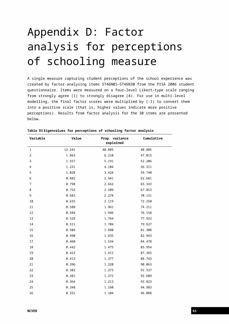
Table F4 Results for student-level predictors of university enrolment
Student attribute Categories df Joint Wald χ2 Model 3 (Final model, n = 5651)
Model 1 Model 2 Wald χ2 Coeff. SE Odds Ratio
Student demographics
Gender Male [R] 1 3.78 3.83 6.57Female 0.248 0.097 1.28
Indigenous status
Indigenous [R] 1 0.13 d
Not indigenous
Length of in-country residence
Australian-born [R] 2 1.46 2.76
First-generation
Foreign-born
Home language English [R] 1 1.88 2.05
Not English
SES Continuous 1 1.97 2.13
Academic achievement
Acad. achievement
Continuous 1 37.56 43.03 44.06 0.506 0.076 1.66
Y12 completion status
Not completed [R] 1 15.89 17.11 20.11
Completed 1.293 0.288 3.64TER quartile No TER [R] 4 355.44 391.64 409.28
TER Q1 (lowest) 0.994 0.15 2.70TER Q2 2.493 0.158 12.10TER Q3 3.241 0.234 25.56TER Q4 (highest) 4.348 0.329 77.32
Aspirations and perceptions
Educ. aspirations
Other unspecified [R]
3 74.58 90.89 112.97
No tertiary study -0.259 0.225 0.77
Apprenticeship -0.644 0.247 0.53University 0.98 0.142 2.66
Perceptions of schooling
Continuous 1 13.86 9.99 13.73 0.208 0.056 1.23
NCVER 61
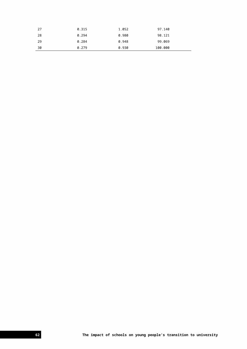
Table F5 Results for school-level predictors of university enrolment
School attribute Categories df Joint Wald χ2 Model 3 (Final model, n = 352)
Model 1 Model 2 Wald χ2 Coeff. SE Odds Ratio
School sector Government [R] 2 4.73 7.64 9.97Catholic 0.505 0.161 1.66Independent 0.164 0.226 1.18
School location Not metropolitan [R] 1 2.30 1.10
Metropolitan
School demographics
Size Continuous 1 0.56 d
SES Continuous 1 1.48 6.55 11.16 0.278 0.083 1.32Acad. achievement
Continuous 1 1.42 d
Gender mix Co-ed [R] 2 0.88 0.81
All male
All female
LBOTE quartile No LBOTE students 4 12.21 13.06 42.93LBOTE Q1 (lowest) 0.247 0.230 1.28
LBOTE Q2 0.458 0.163 1.58LBOTE Q4 0.423 0.225 1.53
LBOTE Q4 (highest)
1.117 0.173 3.06
Resources and capacity
Class size Large (> 20) [R] 1 0.85 d
Small (≤ 20)
Student–teacher ratio
Continuous 1 0.50 d
Degree of teacher shortage
Continuous 1 0.55 d
Prop. certified teachers
Continuous 1 0.30 d
Prop. highly-qual. teachers
Continuous 1 0.60 d
Primary resource base
Government [R] 1 0.81 d
Non-government
Quality of educ. materials
Continuous 1 0.04 d
Continued next page
62 The impact of schools on young people’s transition to university
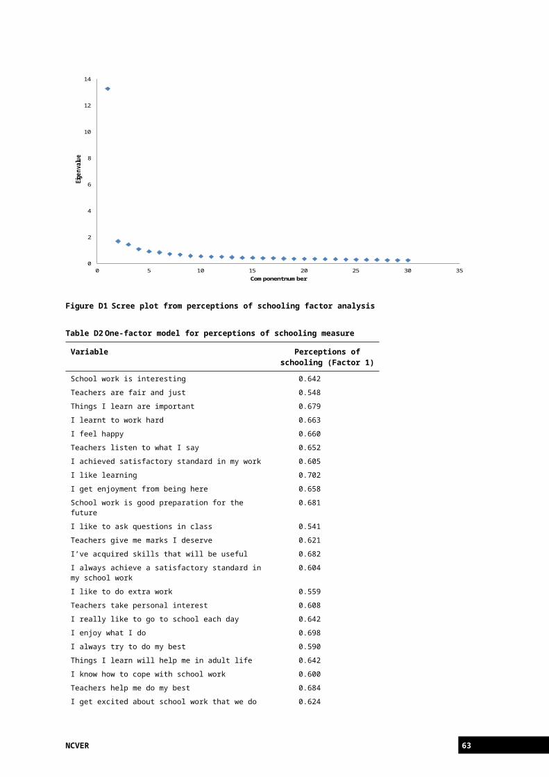
School attribute Categories df Joint Wald χ2 Model 3 (Final model, n = 352)
Model 1 Model 2 Wald χ2 Coeff. SE Odds Ratio
Academic orientation
Acad. press. from parents
Weak [R] 1 0.25 d
Strong
Student selection criteria
At least one prereq. [R]
2 3.37 2.42
Considered
Not considered
Use of streaming For some subjects [R]
2 0.70 d
For no subjects
For all subjects
Exposure to work
For more than half of students [R]
2 1.61 0.32
For half or less of students
Not offered
School autonomyResp. for resources
Continuous 1 0.09 d
Resp. for curriculum
Continuous 1 5.54 3.35
Business influence on curr.
No influence [R] 2 1.03 d
Minor influence
Considerable influence
Providing for student needs
Extracurricular activities
Continuous 1 1.78 d
Career guidance Counsellor-based [R]
1 2.15 0.60
Teacher-based
Perceptions of schooling
Continuous 1 0.53 d
CompetitionTwo or more schools [R]
2 5.71 4.97 6.53
One other school 0.335 0.216 1.40
No other school 0.567 0.271 1.76
NCVER 63
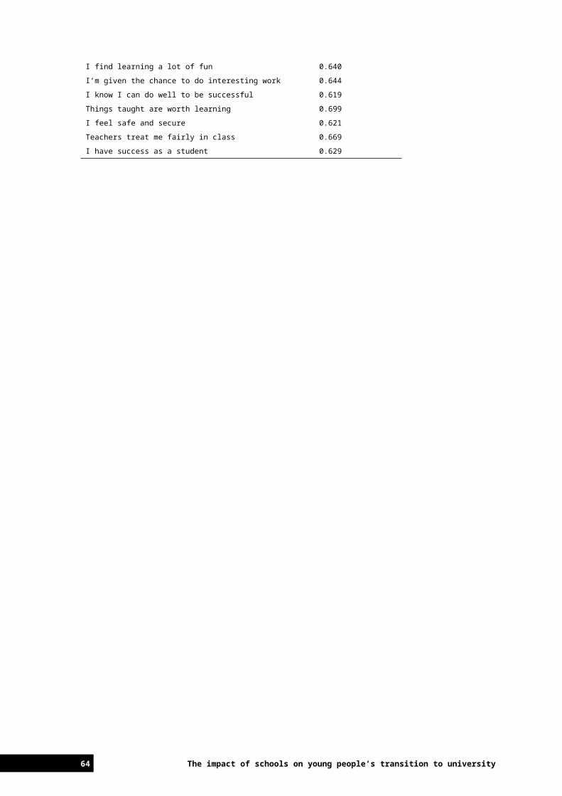
Appendix G: Information on the Logistic scaleFigure 10 in the body of the report depicts the components of the total university enrolment effect by performance cluster. The challenge is that the effect for each school is measured on the logistic scale, whereas the probability of university enrolment is measured on a linear scale between 0 and 1. While units on the logistic scale can be converted probabilities (see figure G1 and the corresponding table G1), this conversion only applies to the total university enrolment effect, but not to its individual components. Thus, figure 10 was not converted into a probability scale.
Figure G1 Conversion graph of logistic scale to linear predictor
Table G1Conversion table of logistic scale to linear predictor
Linear predictor Probability of university enrolment
-2.0 0.12
-1.5 0.18
-1.0 0.27
-0.5 0.38
0.0 0.50
0.5 0.62
1.0 0.73
1.5 0.82
2.0 0.88
2.5 0.92
3.0 0.95
3.5 0.97
4.0 0.98
64 The impact of schools on young people’s transition to university
0.00000
0.20000
0.40000
0.60000
0.80000
1.00000
-2.0 -1.5 -1.0 -0.5 0.0 0.5 1.0 1.5 2.0 2.5 3.0 3.5 4.0
Probability of attending university


![A arXiv:1702.04649v2 [cs.LG] 21 Feb 2017 · Mevlana Gemici , Chia-Chun Hung , Adam Santoro , Greg Wayne Shakir Mohamed, Danilo J. Rezende, David Amos, Timothy Lillicrap DeepMind,](https://static.fdocuments.us/doc/165x107/5e14d37715eb2361f5145a9e/a-arxiv170204649v2-cslg-21-feb-2017-mevlana-gemici-chia-chun-hung-adam.jpg)