SIMULATIONOFGROUND-WATERFLOWINTHEIRWIN … · Table 1. Transmissivity and hydraulic conductivity...
80
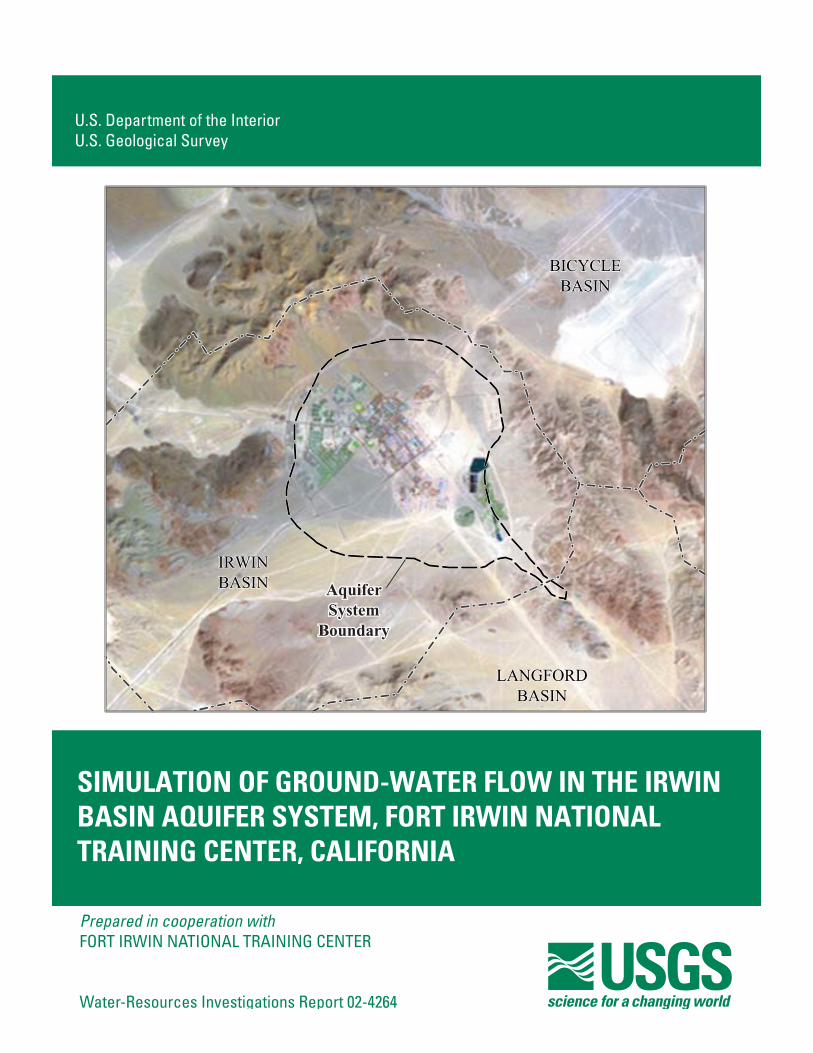
U.S. Department of the Interior U.S. Geological Survey Water-Resources Investigations Report 02-4264 SIMULATION OF GROUND-WATER FLOW IN THE IRWIN BASIN AQUIFER SYSTEM, FORT IRWIN NATIONAL TRAINING CENTER, CALIFORNIA Prepared in cooperation with FORT IRWIN NATIONAL TRAINING CENTER IRWIN BASIN IRWIN BASIN BICYCLE BASIN BICYCLE BASIN LANGFORD BASIN LANGFORD BASIN Aquifer System Boundary Aquifer System Boundary
Transcript of SIMULATIONOFGROUND-WATERFLOWINTHEIRWIN … · Table 1. Transmissivity and hydraulic conductivity...
U.S. Department of the InteriorU.S. Geological Survey
Water-Resources Investigations Report 02-4264
SIMULATION OF GROUND-WATER FLOW IN THE IRWINBASIN AQUIFER SYSTEM, FORT IRWIN NATIONALTRAINING CENTER, CALIFORNIA
Prepared in cooperation withFORT IRWIN NATIONAL TRAINING CENTER
IRWINBASINIRWINBASIN
BICYCLEBASIN
BICYCLEBASIN
LANGFORDBASIN
LANGFORDBASIN
AquiferSystem
Boundary
AquiferSystem
Boundary
Simulation of Ground-Water Flow in the Irwin Basin Aquifer System, Fort Irwin National Training Center, California
By Jill N.Densmore
U.S. GEOLOGICAL SURVEY
Water-Resources Investigations Report 02-4264
Prepared in cooperation with the
FORT IRWIN NATIONAL TRAINING CENTER
5010
-03
Sacramento, California2003
U.S. DEPARTMENT OF THE INTERIOR
GALE A. NORTON, SecretaryU.S. GEOLOGICAL SURVEY
Charles G. Groat, DirectorAny use of trade, product, or firm names in this publication is for descriptive purposes only and does not imply endorsement by the U.S. Government.
For additional information write to:
District ChiefU.S. Geological Survey6000 J Street– Suite 2012Sacramento, California 95819-6129http://ca.water.usgs.gov
Contents
iii
CONTENTS
Abstract
................................................................................................................................................................ 1Introduction .......................................................................................................................................................... 2
Location and Description of Study Area..................................................................................................... 2Acknowledgments....................................................................................................................................... 5
Geohydrology....................................................................................................................................................... 5Geologic Description of Aquifer System.................................................................................................... 6Faults and Ground-Water Boundaries......................................................................................................... 6Aquifer Properties ....................................................................................................................................... 11
Hydraulic Conductivity and Transmissivity ...................................................................................... 11Storage Coefficient ............................................................................................................................ 12Natural Recharge and Discharge........................................................................................................ 12
Ground-Water Pumpage, Water Use, and Artificial Recharge ................................................................... 13Ground-Water Levels and Movement......................................................................................................... 15Ground-Water Quality ................................................................................................................................ 23
Ground-Water Flow Model.................................................................................................................................. 25Model Grid .................................................................................................................................................. 26Model Boundaries ....................................................................................................................................... 32Aquifer Properties ....................................................................................................................................... 33
Hydraulic Conductivity and Transmissivity ...................................................................................... 33Vertical Leakance .............................................................................................................................. 35Storage Coefficient ............................................................................................................................ 38
Simulation of Recharge............................................................................................................................... 38Natural Recharge................................................................................................................................ 42Artificial Recharge ............................................................................................................................. 42
Simulation of Discharge.............................................................................................................................. 42Model Calibration ....................................................................................................................................... 48
Steady-State Model ............................................................................................................................ 49Transient-State Model........................................................................................................................ 49
Model Sensitivity ........................................................................................................................................ 57Simulated Effects of Future Pumpage......................................................................................................... 60Ground-Water Flow Directions and Traveltimes........................................................................................ 62Limitations of the Model............................................................................................................................. 66
Summary and Conclusions................................................................................................................................... 66Selected references............................................................................................................................................... 68
FIGURES
Figure 1. Map showing Mojave Desert region and location of study area at Fort Irwin National Training Center, California................................................................................................................ 3
Figure 2. Map showing generalized geologic map of the Irwin Basin, Fort Irwin National Training Center, California............................................................................................................................... 4
Figure 3. Generalized geology across the Irwin Basin, Fort Irwin National Training Center, California ........ 7Figure 4. Map showing altitude of the basement complex and boundaries of model layers for the Irwin
Basin, Fort Irwin National Training Center, California..................................................................... 10Figure 5. Map showing location of production and other observation wells and sources of recharge
in the Irwin Basin, Fort Irwin National Training Center, California ................................................. 14Figure 6. Graph showing pumpage and recharge, and water-level altitudes in selected wells in the
Irwin Basin, Fort Irwin National Training Center, California, 1941–99 ........................................... 19Figure 7. Map showing altitude of water table and generalized direction of ground-water movement
for selected wells in the Irwin Basin, Fort Irwin National Training Center, California .................... 20Figure 8. Map showing areal distribution of the average dissolved-solids concentrations in ground
water from shallow water-table wells and production wells in Irwin Basin, Fort Irwin National Training Center, California................................................................................................................ 24
Figure 9. Map showing local model grid of the Irwin Basin and the regional model grid of the Fort Irwin National Training Center, California ................................................................................................. 27
Figure 10. Map showing model grid and location of the model boundaries of the Irwin Basin, Fort Irwin National Training Center, California ................................................................................................. 28
Figure 11. Cross-sectional view of model layers, hydraulic conductivities, and boundary conditions of the Irwin Basin, Fort Irwin National Training Center, California ........................................................... 29
Figure 12. Maps showing areal distribution of zones of aquifer properties of the ground-water flow model of the Irwin Basin, Fort Irwin National Training Center, California................................................. 34
Figure 13. Maps showing areal distribution of hydraulic conductivity for layer 1 and layer 2 in the model of the Irwin Basin, Fort Irwin National Training Center, California................................................. 36
Figure 14. Map showing areal distribution of vertical leakance (Vcont) in the Irwin Basin, Fort Irwin National Training Center, California ................................................................................................. 39
Figure 15. Map showing areal distribution of storage coefficients for layer 1and layer 2 in the model of Irwin Basin, Fort Irwin National Training Center, California ........................................................... 40
Figure 16. Map showing areal distribution of natural and artificial recharge for model layer 1 in the model of the Irwin Basin, Fort Irwin National Training Center, California................................................. 43
Figure 17. Annual pumpage from the Irwin, Bicycle, and Langford Basins, Fort Irwin National Training Center, California, 1941–1999............................................................................................ 48
Figure 18. Map showing measured water levels for 1941–43 and simulated hydraulic heads for steady-state conditions for model layer 1 of the Irwin Basin, Fort Irwin National Training Center, California............................................................................................................................... 50
Figure 19. Map showing measured water levels in 1994 and simulated hydraulic heads for transient conditions, layer 1 in the model of the Irwin Basin, Fort Irwin National Training Center, California ........................................................................................................................................... 52
Figure 20. Graph showing simulated hydraulic head and measured water levels (1994) in selected wells in the Irwin Basin, Fort Irwin National Training Center, California ..................................................... 53
Figure 21. Graphs showing measured water levels and simulated hydraulic heads for selected wells in the Irwin Basin, Fort Irwin National Training Center, California ........................................................... 54
iv Figures
Figure 22. Graph showing ground-water recharge to, and discharge from, the Irwin Basin, Fort Irwin National Training Center, California ................................................................................................. 58
Figure 23. Graphs showing results of sensitivity analysis of specific yield and storage coefficient, vertical leakance and fault hydraulic characteristics, and hydraulic conductivity for 1994 conditions in the model of the Irwin Basin, Fort Irwin National Training Center, California ................................ 59
Figure 24. Map showing simulated hydraulic heads for 2050 and 1999 in the Irwin Basin, Fort Irwin National Training Center, California ................................................................................................. 61
Figure 25. Graphs showing simulated hydraulic heads and measured water levels for selected wells in the Irwin Basin, Fort Irwin National Training Center, California ........................................................... 62
Figure 26. Map showing simulated pathlines using particle tracking to determine ground-water movement in the Irwin Basin, Fort Irwin National Training Center, California ................................................. 64
Figures v
vi
Tables
T
ABLES
Table 1. Transmissivity and hydraulic conductivity estimated from specific-capacity data from
wells in the Irwin Basin, Fort Irwin National Training Center, California ........................................... 11
Table 2. Annual ground-water pumpage for the Irwin, Bicycle, and Langford Basins, Fort Irwin National Training Center, California, 1941–99 ..................................................................................... 16
Table 3. Total annual pumpage from the Irwin, Bicycle, and Langford Basins, and range of estimated wastewater recharge calculated from wastewater inflow, potential evaporation and evapotranspiration in the Irwin Basin, Fort Irwin National Training Center, California, 1941–99 ...... 17
Table 3. Total annual pumpage from the Irwin, Bicycle, and Langford Basins, and range of estimated wastewater recharge calculated from wastewater inflow, potential evaporation and evapotranspiration in the Irwin Basin, Fort Irwin National Training Center, California, 1941–99 ...... 17
Table 4. Final values for boundary head and hydraulic conductance used in the general-head boundary package of the model of Irwin Basin, Fort Irwin National Training Center, California. ...... 33
Table 5. Summary of initial and final parameter estimates used in the ground-water flow model of Irwin Basin, Fort Irwin National Training Center, California........................................................... 38
Table 6. Summary of artificial recharge and total artificial recharge from wastewater and irrigation-return flow by sources and range of initial and final estimates of recharge in the Irwin Basin, Fort Irwin National Training Center, California, 1941–99............................................... 44
Table 7. Simulated water budgets for steady-state (pre-1941), transient (1999), and predictive (2050) conditions in the Irwin Basin, Fort Irwin National Training Center, California....... 57
Table 8. Aquifer parameter, model-calibrated value, and range of parameter values used in sensitivity analysis of the ground-water flow model of the Irwin Basin, Fort Irwin National Training Center, California.................................................................................................................... 60
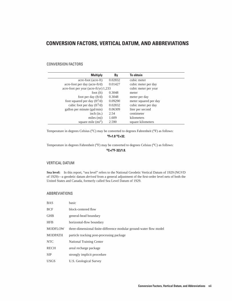
Conversion Factors, Vertical Datum, and Abbreviations
vii
CONVERSION F
ACTORS, VERTICAL DA
TUM, AND ABBREVIA
TIONS
CONVERSION F
ACTORS
T
emperature in degrees Celsius (
o
C) may be con
verted to degrees Fahrenheit (
o
F) as follo
ws:
o
F=1.8
o
C+32.
T
emperature in degrees Fahrenheit (
o
F) may be con
verted to degrees Celsius (
o
C) as follo
ws:
o
C=(
o
F-32)/1.8.
VERTICAL DA
TUM
Sea le
vel:
In this report, “sea level” refers to the National Geodetic Vertical Datum of 1929 (NGVD of 1929)—a geodetic datum
derived
from a general adjustment of the first-order level nets of both the United States and Canada, formerly called Sea Level Datum of 1929.
ABBREVIA
TIONS
B
AS basic
BCF block-centered flow
GHB general-head boundary
HFB horizontal-flow boundary
MODFLOW three-dimensional finite-difference modular ground-water flow model
MODPATH particle tracking post-processing package
NTC National Training Center
RECH areal recharge package
SIP strongly implicit procedure
USGS U.S. Geological Survey
Multiply
By
T
o obtain
acre-foot (acre-ft)
0.02832
cubic meter
acre-foot per day (acre-ft/d)
0.01427
cubic meter per day
acre-foot per year (acre-ft/yr)
1,233
cubic meter per year
foot (ft)
0.3048
meter
foot per day (ft/d)
0.3048
meter per day
foot squared per day (ft
2
/d)
0.09290
meter squared per day
cubic foot per day (ft
3
/d)
0.02832
cubic meter per day
g
allon per minute (gal/min) 0.06309 liter per secondinch (in.) 2.54 centimeter
miles (mi) 1.609 kilometerssquare mile (mi
2
)
2.590
square kilometers
viii
Well-Numbering System
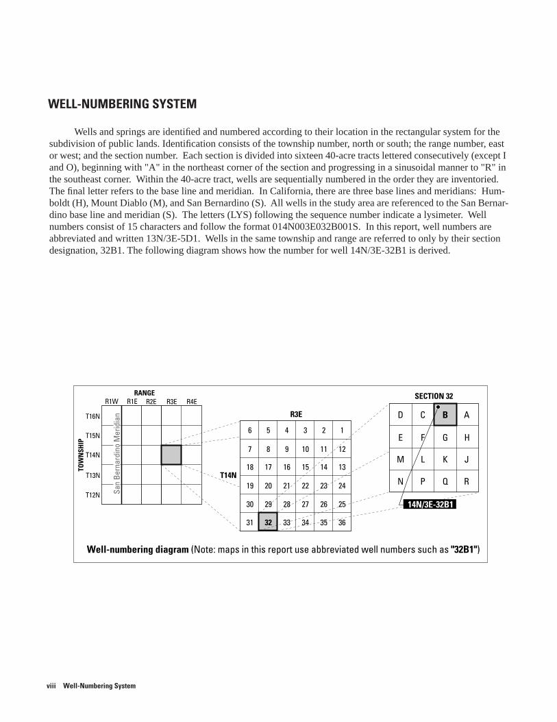
WELL-NUMBERING SYSTEM
W
ells and springs are identified and numbered according to their location in the rectangular system for the subdivision of public lands. Identification consists of the township number, north or south; the range number, east or west; and the section number. Each section is divided into sixteen 40-acre tracts lettered consecutively (except I and O), beginning with "A" in the northeast corner of the section and progressing in a sinusoidal manner to "R" in the southeast corner. Within the 40-acre tract, wells are sequentially numbered in the order they are inventoried. The final letter refers to the base line and meridian. In California, there are three base lines and meridians: Hum-boldt (H), Mount Diablo (M), and San Bernardino (S). All wells in the study area are referenced to the San Bernar-dino base line and meridian (S). The letters (LYS) following the sequence number indicate a lysimeter. Well numbers consist of 15 characters and follow the format 014N003E032B001S. In this report, well numbers are abbreviated and written 13N/3E-5D1. Wells in the same township and range are referred to only by their section designation, 32B1. The following diagram shows how the number for well 14N/3E-32B1 is derived.
R3E R4E
T14N
T15N
T16N
R2ERANGE
TOW
NSH
IP
R1ER1W
T13N
T12N
R3E
Well-numbering diagram (Note: maps in this report use abbreviated well numbers such as "32B1")
San
Bern
ardi
noM
erid
ian
SECTION 32
T14N
14N/3E-32B1
D C B A
E F G H
M L K J
N P Q R
6
7
18
19
30
31
5
8
17
20
29
32
4
9
16
21
28
33
3
10
15
22
27
34
2
11
14
23
26
35
1
12
13
24
25
36
Simulation of Ground-Water Flow in the Irwin Basin Aquifer System, Fort Irwin National Training Center, California
By Jill N. Densmore
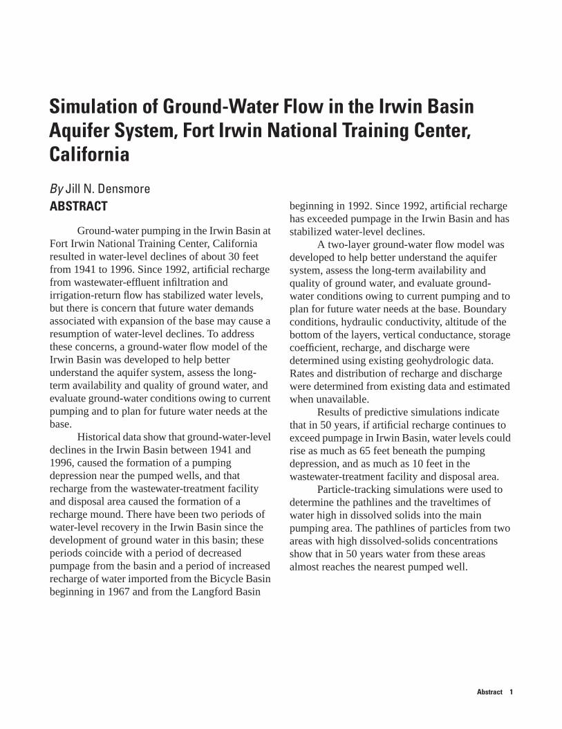
ABSTRACTGround-water pumping in the Irwin Basin at Fort Irwin National Training Center, California resulted in water-level declines of about 30 feet from 1941 to 1996. Since 1992, artificial recharge from wastewater-effluent infiltration and irrigation-return flow has stabilized water levels, but there is concern that future water demands associated with expansion of the base may cause a resumption of water-level declines. To address these concerns, a ground-water flow model of the Irwin Basin was developed to help better understand the aquifer system, assess the long-term availability and quality of ground water, and evaluate ground-water conditions owing to current pumping and to plan for future water needs at the base.
Historical data show that ground-water-level declines in the Irwin Basin between 1941 and 1996, caused the formation of a pumping depression near the pumped wells, and that recharge from the wastewater-treatment facility and disposal area caused the formation of a recharge mound. There have been two periods of water-level recovery in the Irwin Basin since the development of ground water in this basin; these periods coincide with a period of decreased pumpage from the basin and a period of increased recharge of water imported from the Bicycle Basin beginning in 1967 and from the Langford Basin
beginning in 1992. Since 1992, artificial recharge has exceeded pumpage in the Irwin Basin and has stabilized water-level declines.
A two-layer ground-water flow model was developed to help better understand the aquifer system, assess the long-term availability and quality of ground water, and evaluate ground-water conditions owing to current pumping and to plan for future water needs at the base. Boundary conditions, hydraulic conductivity, altitude of the bottom of the layers, vertical conductance, storage coefficient, recharge, and discharge were determined using existing geohydrologic data. Rates and distribution of recharge and discharge were determined from existing data and estimated when unavailable.
Results of predictive simulations indicate that in 50 years, if artificial recharge continues to exceed pumpage in Irwin Basin, water levels could rise as much as 65 feet beneath the pumping depression, and as much as 10 feet in the wastewater-treatment facility and disposal area.
Particle-tracking simulations were used to determine the pathlines and the traveltimes of water high in dissolved solids into the main pumping area. The pathlines of particles from two areas with high dissolved-solids concentrations show that in 50 years water from these areas almost reaches the nearest pumped well.
Abstract 1
INTRODUCTION
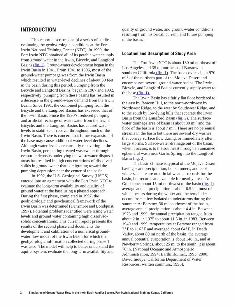
This report describes one of a series of studies evaluating the geohydrologic conditions at the Fort Irwin National Training Center (NTC). In 1999, the Fort Irwin NTC obtained all of its potable water supply from ground water in the Irwin, Bicycle, and Langford Basins (fig. 1). Ground-water development began in the Irwin Basin in 1941. From 1941 to 1996, most of the ground-water pumpage was from the Irwin Basin which resulted in water-level declines of about 30 feet in the basin during this period. Pumping from the Bicycle and Langford Basins, began in 1967 and 1992, respectively; pumping from these basins has resulted in a decrease in the ground-water demand from the Irwin Basin. Since 1991, the combined pumping from the Bicycle and the Langford Basins has exceeded that of the Irwin Basin. Since the 1990’s, reduced pumping and artificial recharge of wastewater from the Irwin, Bicycle, and the Langford Basins has caused water levels to stabilize or recover throughout much of the Irwin Basin. There is concern that future expansion of the base may cause additional water-level declines. Although water levels are currently recovering in the Irwin Basin, percolating treated wastewater through evaporite deposits underlying the wastewater-disposal areas has resulted in high concentrations of dissolved solids in ground water that is migrating toward the pumping depression near the center of the basin.
In 1992, the U.S. Geological Survey (USGS) entered into an agreement with the Fort Irwin NTC to evaluate the long-term availability and quality of ground water at the base using a phased approach. During the first phase, completed in 1997, the geohydrologic and geochemical framework of the Irwin Basin was determined (Densmore and Londquist, 1997). Potential problems identified were rising water levels and ground water containing high dissolved-solids concentrations. This current report presents the results of the second phase and documents the development and calibration of a numerical ground-water flow model of the Irwin Basin for which the geohydrologic information collected during phase 1 was used. The model will help to better understand the aquifer system, evaluate the long-term availability and
quality of ground water, and ground-water conditions resulting from historical, current, and future pumping in the basin.
Location and Description of Study Area
The Fort Irwin NTC is about 130 mi northeast of Los Angeles and 35 mi northeast of Barstow in southern California (fig. 1). The base covers about 970 mi2 of the northern part of the Mojave Desert and encompasses several ground-water basins. The Irwin, Bicycle, and Langford Basins currently supply water to the base (fig. 1).
The Irwin Basin has a fairly flat floor bordered to the east by Beacon Hill, to the north-northwest by Northwest Ridge, to the west by Southwest Ridge, and to the south by low-lying hills that separate the Irwin Basin from the Langford Basin (fig. 2). The surface-water drainage area of basin is about 30 mi2 and the floor of the basin is about 7 mi2. There are no perennial streams in the basin but there are several dry washes that convey surface flow during, or immediately after, large storms. Surface-water drainage out of the basin, when it occurs, is to the southeast through an unnamed ephemeral wash near Garlic Spring into the Langford Basin (fig. 2).
The basin climate is typical of the Mojave Desert having scant precipitation, hot summers, and cool winters. There are no official weather records for the basin, but records are available for nearby areas. At Goldstone, about 15 mi northwest of the basin (fig. 1), average annual precipitation is about 6.5 in., most of which occurs during the winter and the remainder occurs from a few isolated thunderstorms during the summer. At Barstow, 30 mi southwest of the basin, average annual precipitation is about 4.4 in. Between 1973 and 1999, the annual precipitation ranged from about 2 in. in 1975 to about 11.5 in. in 1983. Between 1940 and 1999, temperatures at Barstow ranged from 3 F to 116 F and averaged about 64 F. In Death Valley, about 80 mi north of the basin, the average annual potential evaporation is about 148 in., and at Newberry Springs, about 25 mi to the south, it is about 76 in. (National Oceanic and Atmospheric Administration, 1994; EarthInfo, Inc., 1995, 2000; David Inouye, California Department of Water Resources, written commun., 1996).
° ° °
2 Simulation of Ground-Water Flow in the Irwin Basin Aquifer System, Fort Irwin National Training Center, California
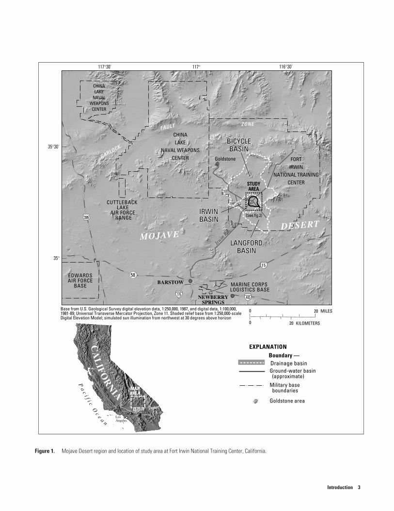
Figure 1. Mojave Desert region and location of study area at Fort Irwin National Training Center, California.
STUDYAREA
BARSTOW
NEWBERRYSPRINGS
117°30' 117° 116°30'
35°
35°30'
IRWINBASIN
BICYCLEBASIN
LANGFORDBASIN
IRWINBASIN
BICYCLEBASIN
LANGFORDBASIN
EXPLANATION
Drainage basinGround-water basin
(approximate)
Military baseboundaries
Goldstone area
Boundary —
58
LosAngeles
Irwin
Rd
FORTIRWIN
NATIONAL TRAININGCENTER
CHINALAKE
NAVAL WEAPONSCENTER
CHINALAKE
NAVALWEAPONS
CENTER
GARLOCK
FAULT ZONE
CUTTLEBACKLAKE
AIR FORCERANGE
EDWARDSAIR FORCE
BASE MARINE CORPSLOGISTICS BASE
Goldstone
(See fig.2)
MAPAREAMAPAREA
Mojave DesertMojave Desert
MOJAVEDESERT
Base from U.S. Geological Survey digital elevation data, 1:250,000, 1987, and digital data, 1:100,000,1981-89; Universal Transverse Mercator Projection, Zone 11. Shaded relief base from 1:250,000-scaleDigital Elevation Model; simulated sun illumination from northwest at 30 degrees above horizon
0 20
0 20
MILES
KILOMETERS
15
15 40
395
CA
LIF
OR
NIA
Pa
ci f i c
Oc
e a
n
Introduction 3
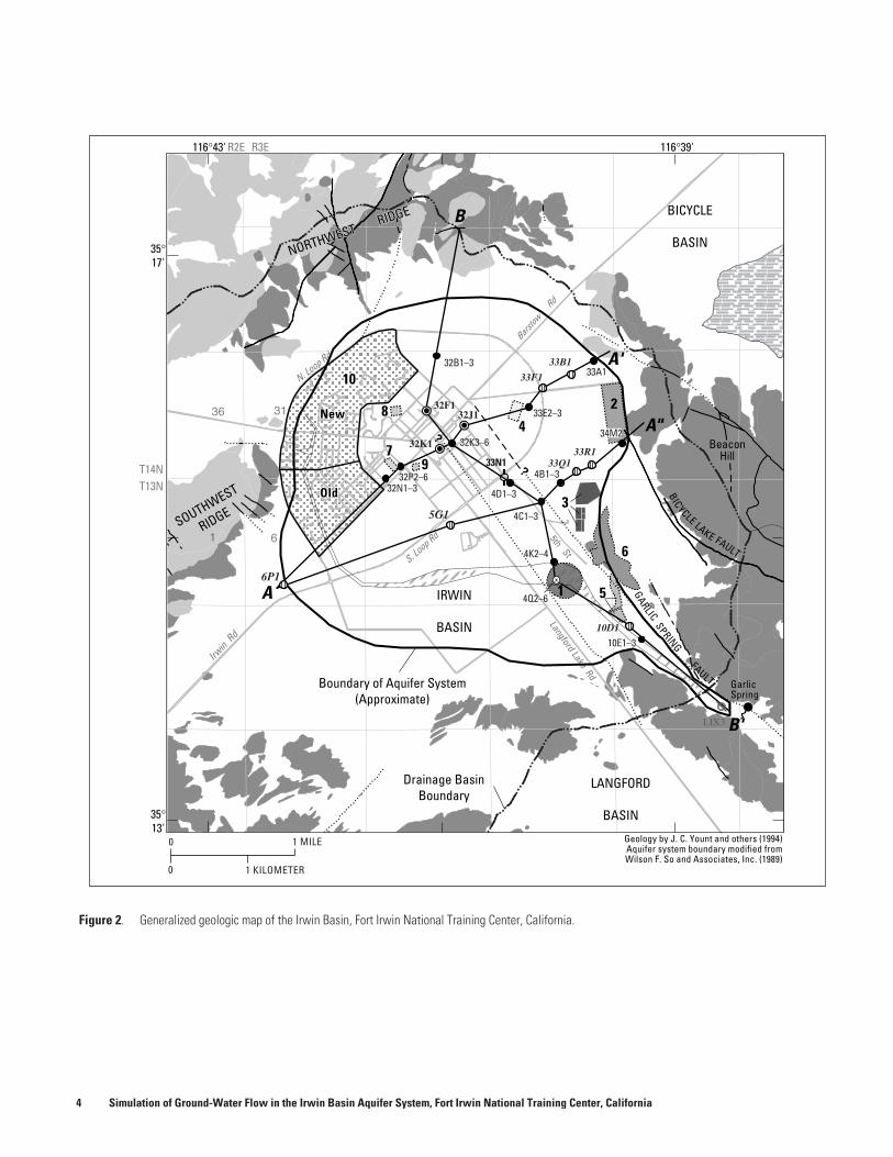
Figure 2. Generalized geologic map of the Irwin Basin, Fort Irwin National Training Center, California.
Barstow
Rd
Irwin
Rd
N. Loop Rd
S. Loop Rd
Langford LakeRd
5thSt
B
A'
A
A"
B'
New
Old
New
Old BICYCLE LAKE FAULT
Drainage BasinBoundary
Boundary of Aquifer System(Approximate)
LANGFORD
BASIN
IRWIN
BASIN
BICYCLE
BASINNORTHWEST
RIDGE
NORTHWESTRIDGE
SOUTHWEST
RIDGE
BeaconHill
BeaconHill
GarlicSpring
1
2
3
4
6
7
8
9
1010
5 GARLICSPRING
FAULT
32J132F1
32K1
LIX3
33F1
33Q1
10D1
33R1
33B1
6P1
32B1–3
4B1–3
4D1–3
4C1–3
4K2–4
4Q2–6
10E1–310E1–3
33A1
34M2
33N132P2–6
32K3–6
32N1–3
116°39'116°43'
35°17'
35°13'
T14NT13N
R2E R3E
5G1
33E2–3
1 MILE
1 KILOMETER
0
0
Geology by J. C. Yount and others (1994)Aquifer system boundary modified fromWilson F. So and Associates, Inc. (1989)
4 Simulation of Ground-Water Flow in the Irwin Basin Aquifer System, Fort Irwin National Training Center, California
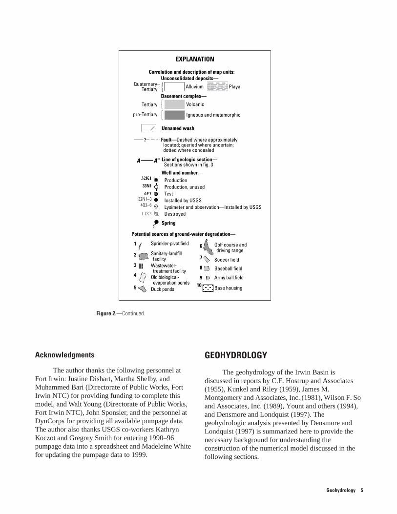
Figure 2.—Continued.
32N1–34Q2–6
LIX3
32K1
6P1
A"A
Golf course anddriving range
Soccer field
Baseball field
Army ball field
Base housing
Correlation and description of map units:
Potential sources of ground-water degradation—
Unconsolidated deposits—
Basement complex—
Well and number—
Spring
Unnamed wash
Fault—Dashed where approximatelylocated; queried where uncertain;dotted where concealed
Line of geologic section—Sections shown in fig. 3
?
Quaternary–Tertiary
Tertiary
pre-Tertiary
Alluvium
Volcanic
Igneous and metamorphic
Playa
EXPLANATION
ProductionProduction, unused
Sprinkler-pivot field
Sanitary-landfillfacility
Wastewater-treatment facility
Old biological-evaporation ponds
Duck ponds
TestInstalled by USGSLysimeter and observation—Installed by USGSDestroyed
1
2
3
4
5
6
7
8
910
33N1
Acknowledgments
The author thanks the following personnel at Fort Irwin: Justine Dishart, Martha Shelby, and Muhammed Bari (Directorate of Public Works, Fort Irwin NTC) for providing funding to complete this model, and Walt Young (Directorate of Public Works, Fort Irwin NTC), John Sponsler, and the personnel at DynCorps for providing all available pumpage data. The author also thanks USGS co-workers Kathryn Koczot and Gregory Smith for entering 1990–96 pumpage data into a spreadsheet and Madeleine White for updating the pumpage data to 1999.
GEOHYDROLOGY
The geohydrology of the Irwin Basin is discussed in reports by C.F. Hostrup and Associates (1955), Kunkel and Riley (1959), James M. Montgomery and Associates, Inc. (1981), Wilson F. So and Associates, Inc. (1989), Yount and others (1994), and Densmore and Londquist (1997). The geohydrologic analysis presented by Densmore and Londquist (1997) is summarized here to provide the necessary background for understanding the construction of the numerical model discussed in the following sections.
Geohydrology 5
Geologic Description of Aquifer System
The Irwin Basin is filled with as much as 950 ft of unconsolidated deposits that consist of younger alluvium of Quaternary age and older alluvium of late Tertiary to Quaternary age (fig. 3). The deposits are unconsolidated at land surface and become partly consolidated with depth. The unconsolidated deposits are the only water-bearing material in the basin from which appreciable amounts of ground water may be obtained. These deposits are underlain by a basement complex of volcanic rocks of late Tertiary to Quaternary age and igneous and metamorphic rocks of pre-Tertiary age, which convey insignificant amounts of ground water except in areas where they are jointed and fractured.
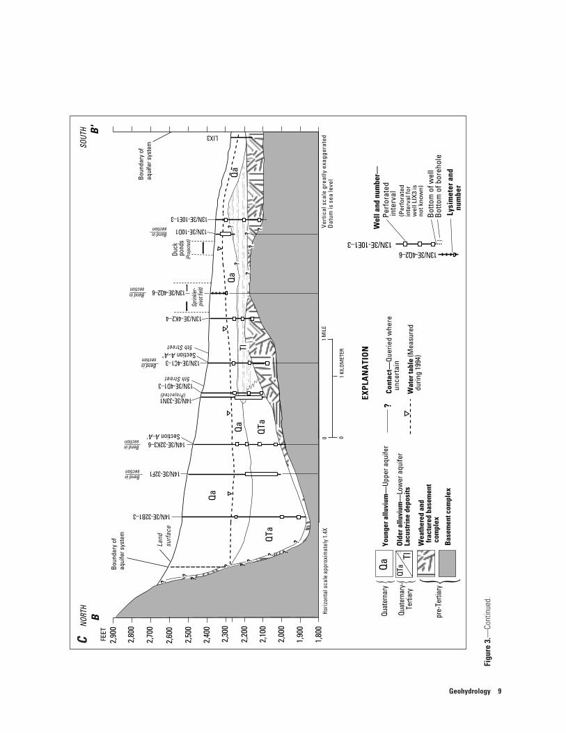
The older alluvium (fig. 3, QTa and Tl) consists of sand, gravel, and clay derived predominantly from granitic material—except in the northern part of the basin, where volcanic material dominates. Where the older alluvium consists predominantly of sand and gravel, it yields moderate amounts of water to wells. However, in the southeastern part of the basin, it consists almost entirely of low-permeability lacustrine deposits (fig. 3, B–B , Tl) of silt and clay. These low-permeability deposits extend from well 14N/3E-33N1 near the center of the basin to well 13N/3E-10E1-3 in the unnamed wash that leads to Garlic Spring, and are bounded by the Garlic Spring Fault on the northeast and an unnamed fault on the southwest.
The younger alluvium (fig. 3, Qa) consists primarily of loose coarse sand and gravel with small amounts of clay. Some thin discontinuous clay lenses overlie the lacustrine deposits within the older alluvium in the area beneath the sprinkler-pivot field in the southeastern part of the basin (fig. 2) and may result in a perched water table in this area. Most of the younger alluvium lies above the water table; however, in areas where it is saturated, primarily in the center of the basin, it yields large quantities of water to wells (as much as to 1,000 gal/min). Wellbore-flow tests of selected base supply wells indicate that most of the water pumped comes from the younger alluvium (Densmore and Londquist, 1997).
The aquifer system in the Irwin Basin consists of an upper aquifer and a lower aquifer. The upper aquifer is unconfined and is contained within the saturated part of the younger alluvium. This aquifer reaches a
maximum thickness of about 200 ft in the west-central part of the basin (fig. 3). The lower aquifer is confined throughout most of the basin and includes the older alluvium. This aquifer reaches a maximum thickness of more than 600 ft in the central part of the basin (fig. 3). Although some water is contained in the underlying basement complex, the effective base of the ground-water system is at the top of basement complex. The altitude of the surface of the basement complex in the Irwin Basin is shown in figure 4.
Faults and Ground-Water Boundaries
Numerous faults have been mapped in the bedrock hills surrounding the basin (Yount and others, 1994) (figs. 2 and 3); they include the Garlic Spring Fault, the Bicycle Lake Fault, and many unnamed faults. Most are buried beneath the unconsolidated deposits and thus, their presence within the basin is largely unknown. Yount and others (1994) mapped the Garlic Spring Fault into the unconsolidated deposits; they suggest that the fault may cut through both the younger and the older alluvium in the southeastern part of the basin. Water-quality and water-level data, presented by Densmore and Londquist (1997), indicate that the Garlic Spring Fault and a parallel unnamed fault may be acting, in part, as a partial barrier to horizontal ground-water flow, primarily in the lower aquifer. The water-quality data indicate that vertical flow is also being impeded on the west side of the Garlic Spring Fault, because of lithologic differences between the younger alluvium and the lacustrine deposits of the older alluvium. Minor compaction and deformation of the water-bearing deposits immediately adjacent to the faults, fault gouge along the fault zone, and cementation of the fault zone by the deposition of minerals from ground water are believed to cause the barrier effect of the faults.
The areal extent of the aquifer system is defined by the intersection of the water table and the surrounding rocks of the basement complex. During predevelopment conditions, the water table was about 2,300 feet above sea level. The boundary of the aquifer system coincides with the 2,300-foot altitude of the basement complex (fig. 4) (the approximate boundary of the basin is shown in figure 2). All the alluvial deposits above this altitude were unsaturated during predevelopment conditions.
′
6 Simulation of Ground-Water Flow in the Irwin Basin Aquifer System, Fort Irwin National Training Center, California
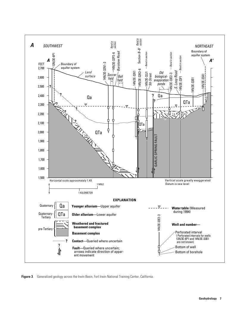
Figure 3. Generalized geology across the Irwin Basin, Fort Irwin National Training Center, California.
Boundary ofaquifer system
Boundary ofaquifer system
14N/
3E-3
2P2–
6
14N/
3E-3
2K1
14N/
3E-3
2K3–
6
14N/
3E-3
2J1
14N/
3E-3
3E2–
3
14N/
3E-3
3F1
14N/
3E-3
3A1
14N/
3E-3
2N1–
3
13N/
3E-6
P1
SOUTHWEST NORTHEAST
?
?
Qa Qa
QTa
QTa
QTa
QTa
2,600
2,700FEET
2,500
2,400
2,300
2,200
2,100
2,000
1,900
1,800
1,700
1,600
1,500
A A'
Soccerfield Ball
field
Sect
ion
B–B'
?
?
Water table (Measuredduring 1994)
? Contact—Queried where uncertain
Fault—Queried where uncertain;arrows indicate direction of appar-ent movement
Well and number—
Perforated interval
Bottom of boreholeBottom of well
Vertical scale greatly exaggeratedHorizontal scale approximately 1.4X
EXPLANATION
14N/
3E-3
3E2–
3
5th
Stre
et
S.Lo
opRo
ad
Bar
stow
Road
Oldbiological-
evaporationponds
}
GA
RLIC
SPRI
NG
FAU
LT
Qa
Basement complex
Younger alluvium—Upper aquifer
Older alluvium—Lower aquifer
Weathered and fracturedbasement complex
Quaternary
Quaternary–Tertiary
{{
{pre-Tertiary
( Perforated intervals for wells13N/3E-6P1 and 14N/3E-33B1are not known)
14N/
3E-3
3B1
0
0 1 MILE Datum is sea level
1 KILOMETER
Bend
inse
ctio
n
Bend
inse
ctio
n
Bend
inse
ctio
n
Bend
inse
ctio
n
Bend
inse
ctio
n
?
?
??
??
?
Landsurface
A
Geohydrology 7
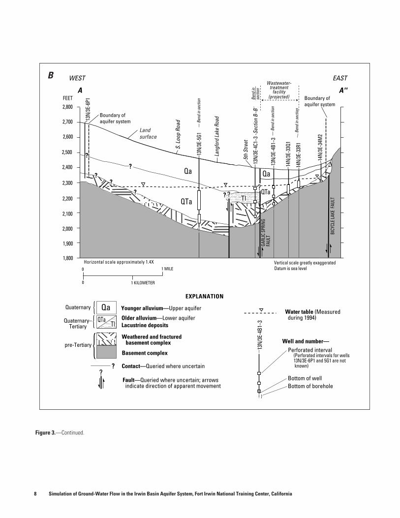
Figure 3.—Continued.
WEST EAST
2,500
FEET
2,400
2,700
2,800
2,600
2,300
2,200
2,100
2,000
1,900
1,800
0
0 1 MILE Datum is sea level
1 KILOMETER
A A''
?
?
?
Vertical scale greatly exaggerated13
N/3E
-4C1
–3-S
ectio
nB–
B'
13N/
3E-5
G1
14N/
3E-3
3Q1
14N/
3E-3
3R1
13N/
3E-4
B1–3
14N/
3E-3
4M2
13N/
3E-6
P1
?
Lang
ford
Lake
Road
5th
Stre
et
S.Lo
opRo
ad
GARL
ICSP
RING
FAUL
T BICY
CLEL
AKE
FAUL
T
13N/
3E-4
B1–3
Qa
QTa
Qa
QTa
Wastewater-treatment
facility(projected)
?
?
Water table (Measuredduring 1994)
? Contact—Queried where uncertain
Fault—Queried where uncertain; arrowsindicate direction of apparent movement
Well and number—Perforated interval
Bottom of boreholeBottom of well
EXPLANATION
}
Qa
Basement complex
Younger alluvium—Upper aquifer
Older alluvium—Lower aquiferLacustrine deposits
Weathered and fracturedbasement complex
Quaternary {{
{pre-Tertiary
Bend
inse
ctio
n
Bend
inse
ctio
n
Bend
inse
ctio
n
Bend
inse
ctio
n
QTaQuaternary–Tertiary
(Perforated intervals for wells13N/3E-6P1 and 5G1 are notknown)
Horizontal scale approximately 1.4X
Tl
Tl?
??
?
Boundary ofaquifer system
Boundary ofaquifer system
Landsurface
B
8 Simulation of Ground-Water Flow in the Irwin Basin Aquifer System, Fort Irwin National Training Center, California
Figu
re 3
.
—Co
ntin
ued.
??
?
??
14N/3E-33N1
14N/3E-32B1–3
14N/3E-32K3–6
14N/3E-32F1
13N/3E-4D1–3
13N/3E-4C1–3
13N/3E-4Q2–6
13N/3E-4K2–4
13N/3E-10D1
13N/3E-10E1–3
Qa
Qa
QaQa
QTa
QTa
Sprin
kler-
pivot
field
Duck
pond
s 13N/3E-10E1–3
SectionA–A"
SectionA–A'
Lysi
met
eran
dnu
mbe
r
Vert
ical
scal
egr
eatly
exag
gera
ted
(Projected)
5thStreet
5thStreet
}
13N/3E-4Q2–6
(Pro
jecte
d)
Bendinsection
Bendinsection
Bendinsection
Bendinsection
Bendinsection
Wat
erta
ble
(Mea
sure
ddu
ring
1994
)
?Co
ntac
t—Q
uerie
dw
here
unce
rtai
n
Wel
land
num
ber—
Perf
orat
edin
terv
al
Bot
tom
ofbo
reho
leB
otto
mof
wel
l
EXPL
AN
ATI
ON
Qa
Bas
emen
tcom
plex
Youn
gera
lluvi
um—
Uppe
raqu
ifer
Old
eral
luvi
um—
Low
eraq
uife
rLa
cust
rine
depo
sits
Wea
ther
edan
dfr
actu
red
base
men
tco
mpl
ex
Quat
erna
ry{ { {
pre-
Terti
ary
(Per
fora
ted
inte
rval
for
wel
lLIX
3is
notk
now
n)
?
?
?
QTa
Quat
erna
ry-
Terti
ary
Horiz
onta
lsca
leap
prox
imat
ely
1.4X
Tl
Tl
001
MIL
ED
atum
isse
ale
vel
1KI
LOM
ETER
?
?
?
?
?
?
SOUT
HNO
RTH
2,60
0
2,70
0
2,90
0
2,80
0
FEET
2,50
0
2,40
0
2,30
0
2,20
0
2,10
0
2,00
0
1,90
0
1,80
0
BB
'
LIX3
?
Boun
dary
ofaq
uife
rsys
tem
Boun
dary
ofaq
uife
rsys
tem
Land
surfa
ce
C
Geohydrology 9
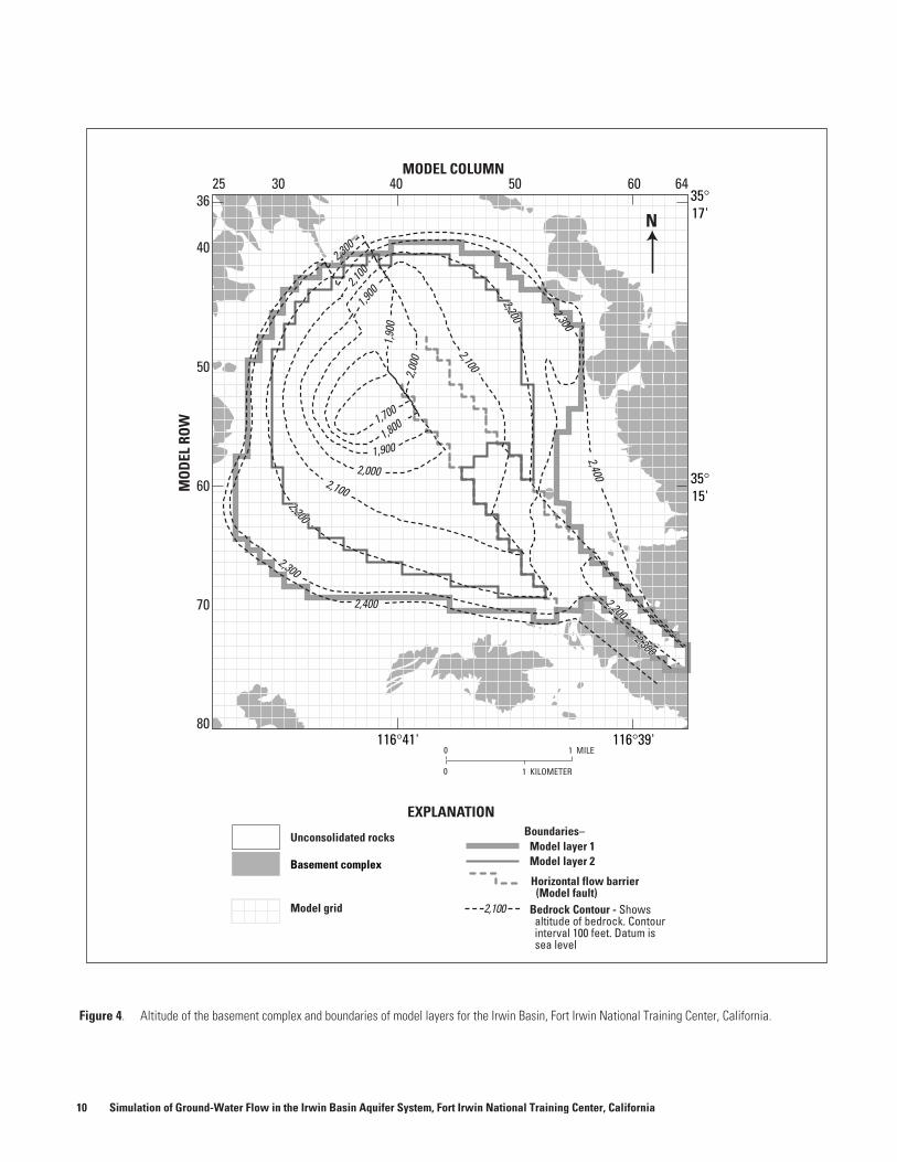
Figure 4. Altitude of the basement complex and boundaries of model layers for the Irwin Basin, Fort Irwin National Training Center, California.
25 30 40 50 6036
40
50
60
70
80
64MODEL COLUMN
MO
DEL
ROW
1,900
2,000
2,2002,200
2,300
2,400
2,00
0
2,2002,200
2,400
1,90
0
1,700
2,100
2,100
2,100
2,300
1,900
1,800
2,300
2,2002,200
2,3002,300
35°15'
116°39'116°41'
35°17'N
0
0 1 KILOMETER
1 MILE
Basement complex
Unconsolidated rocks
Model layer 2
Bedrock Contour - Showsaltitude of bedrock. Contourinterval 100 feet. Datum issea level
2,100
EXPLANATION
Model grid
Model layer 1Boundaries–
Horizontal flow barrier(Model fault)
10 Simulation of Ground-Water Flow in the Irwin Basin Aquifer System, Fort Irwin National Training Center, California
Aquifer Properties
Hydraulic Conductivity and Transmissivity
Hydraulic conductivity is defined as the capacity of a rock or unconsolidated material to transmit water (Heath, 1983). Transmissivity is defined as the rate at which water is transmitted through an aquifer (Heath, 1983) and is equal to the hydraulic conductivity multiplied by the aquifer thickness.
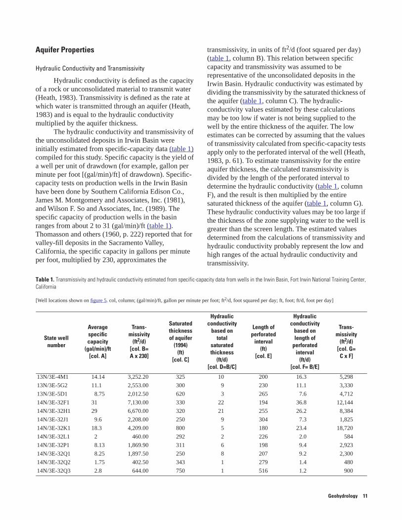
The hydraulic conductivity and transmissivity of the unconsolidated deposits in Irwin Basin were initially estimated from specific-capacity data (table 1) compiled for this study. Specific capacity is the yield of a well per unit of drawdown (for example, gallon per minute per foot [(gal/min)/ft] of drawdown). Specific-capacity tests on production wells in the Irwin Basin have been done by Southern California Edison Co., James M. Montgomery and Associates, Inc. (1981), and Wilson F. So and Associates, Inc. (1989). The specific capacity of production wells in the basin ranges from about 2 to 31 (gal/min)/ft (table 1). Thomasson and others (1960, p. 222) reported that for valley-fill deposits in the Sacramento Valley, California, the specific capacity in gallons per minute per foot, multiplied by 230, approximates the
transmissivity, in units of ft2/d (foot squared per day) (table 1, column B). This relation between specific capacity and transmissivity was assumed to be representative of the unconsolidated deposits in the Irwin Basin. Hydraulic conductivity was estimated by dividing the transmissivity by the saturated thickness of the aquifer (table 1, column C). The hydraulic-conductivity values estimated by these calculations may be too low if water is not being supplied to the well by the entire thickness of the aquifer. The low estimates can be corrected by assuming that the values of transmissivity calculated from specific-capacity tests apply only to the perforated interval of the well (Heath, 1983, p. 61). To estimate transmissivity for the entire aquifer thickness, the calculated transmissivity is divided by the length of the perforated interval to determine the hydraulic conductivity (table 1, column F), and the result is then multiplied by the entire saturated thickness of the aquifer (table 1, column G). These hydraulic conductivity values may be too large if the thickness of the zone supplying water to the well is greater than the screen length. The estimated values determined from the calculations of transmissivity and hydraulic conductivity probably represent the low and high ranges of the actual hydraulic conductivity and transmissivity.
Table 1. Transmissivity and hydraulic conductivity estimated from specific-capacity data from wells in the Irwin Basin, Fort Irwin National Training Center, California
[Well locations shown on figure 5. col, column; (gal/min)/ft, gallon per minute per foot; ft2/d, foot squared per day; ft, foot; ft/d, foot per day]
State well number
Averagespecificcapacity
(gal/min)/ft[col. A]
Trans-missivity
(ft2/d)[col. B=A x 230]
Saturatedthicknessof aquifer
(1994)(ft)
[col. C]
Hydraulicconductivity
based on total
saturatedthickness
(ft/d)[col. D=B/C]
Length of perforated
interval(ft)
[col. E]
Hydraulicconductivity
based onlength of
perforatedinterval
(ft/d)[col. F= B/E]
Trans-missivity
(ft2/d)[col. G=
C x F]
13N/3E-4M1 14.14 3,252.20 325 10 200 16.3 5,298
13N/3E-5G2 11.1 2,553.00 300 9 230 11.1 3,330
13N/3E-5D1 8.75 2,012.50 620 3 265 7.6 4,712
14N/3E-32F1 31 7,130.00 330 22 194 36.8 12,144
14N/3E-32H1 29 6,670.00 320 21 255 26.2 8,384
14N/3E-32J1 9.6 2,208.00 250 9 304 7.3 1,825
14N/3E-32K1 18.3 4,209.00 800 5 180 23.4 18,720
14N/3E-32L1 2 460.00 292 2 226 2.0 584
14N/3E-32P1 8.13 1,869.90 311 6 198 9.4 2,923
14N/3E-32Q1 8.25 1,897.50 250 8 207 9.2 2,300
14N/3E-32Q2 1.75 402.50 343 1 279 1.4 480
14N/3E-32Q3 2.8 644.00 750 1 516 1.2 900
Geohydrology 11
Storage Coefficient
The storage coefficient of an aquifer is the volume of water that is released from or taken into storage per unit surface area per unit change in head (Driscoll, 1986). For this ground-water flow model of Irwin Basin, layer 1 was simulated as an unconfined aquifer and layer 2 was simulated as a confined aquifer in all the modeled areas. For unconfined aquifers, the storage coefficient is virtually equal to the specific yield. Specific yield is the ratio of the volume of water that will drain by gravity per unit volume of the formation. The estimated average specific yield for the upper 150 ft of sediment in Irwin Basin is 0.19, or 19 percent (James M. Montgomery and Associates, Inc., 1981). In unconfined aquifers, water released from storage comes from an actual dewatering of the soil pores and results in lowering of the water table; however, in a confined aquifer, water released from storage comes from expansion of the water and from compression of the aquifer and results in lowering of the potentiometric surface (Heath, 1983, p. 28). Thus, the storage coefficient for a confined aquifer will be much lower than that for an unconfined aquifer.
Natural Recharge and Discharge
Natural recharge in the Irwin Basin is solely from precipitation runoff within the surface-water drainage basin (an area of about 30 mi2) and probably occurs only during and shortly after high-intensity or long-duration storms. Although no precipitation records are available for the Irwin Basin, nearby Barstow and Goldstone areas receive on average only 4.4 and 6.5 in. of rain per year, respectively. Most of the natural recharge likely occurs in the coarse deposits along the normally dry washes, where precipitation runoff from the surrounding bedrock areas is diverted by dikes around the base housing (fig. 2) and temporary buildings that make up the cantonment area near the center of the basin. Recharge to the aquifer system from direct precipitation is considered minimal because precipitation or runoff do not adequately meet evapotranspiration and soil-moisture requirements. Recent work in the upper Mojave Basin by Izbicki and
others (2000) suggests that infiltration does not occur at depths below the root zone except in areas of some intermittent washes.
C.F. Hostrup and Associates (1955) estimated that the average annual recharge from precipitation runoff in the Irwin drainage basin between 1941 and 1951 was about 150 acre-ft/yr. This estimate is based on ground-water pumpage and water-level changes during the 10-year period. Ground water from wells unaffected by artificial recharge in the Irwin Basin does not contain measurable concentrations of tritium (3H) (Densmore and Londquist, 1997), indicating that natural recharge rates through the thick (as much as 270 ft in the northern part of the basin) unsaturated zone are fairly low.
Natural discharge occurs from the ground-water system in the Irwin Basin into the Langford Basin as subsurface underflow beneath the unnamed wash near Garlic Spring (fig. 2). Prior to ground-water development in 1941, ground-water discharge was the only discharge from the basin. Evaporation from the water table was negligible because depth to ground water was more than 10 ft below land surface throughout the basin. Therefore, prior to ground-water development (1941) the ground-water basin was likely in a steady-state condition with natural discharge by subsurface underflow equal to the natural recharge to the basin.
Discharge by subsurface underflow beneath the unnamed wash near Garlic Spring for predevelopment conditions is unknown. However, discharge for 1994, estimated by Densmore and Londquist (1997) using Darcy’s law, was about 85 acre-ft/yr (10,000 ft3/d). This estimate of natural discharge is lower than the natural recharge of 150 acre-ft/yr estimated by C.F. Hostrup and Associates (1955). For predevelopment (steady-state) conditions, recharge should equal discharge; therefore, either the natural recharge is overestimated or the natural discharge from the basin in 1994 underestimates the predevelopment natural discharge. In any case, these estimates indicate that the natural recharge and discharge are fairly low and of the same order of magnitude.
12 Simulation of Ground-Water Flow in the Irwin Basin Aquifer System, Fort Irwin National Training Center, California
Ground-Water Pumpage, Water Use, and Artificial Recharge
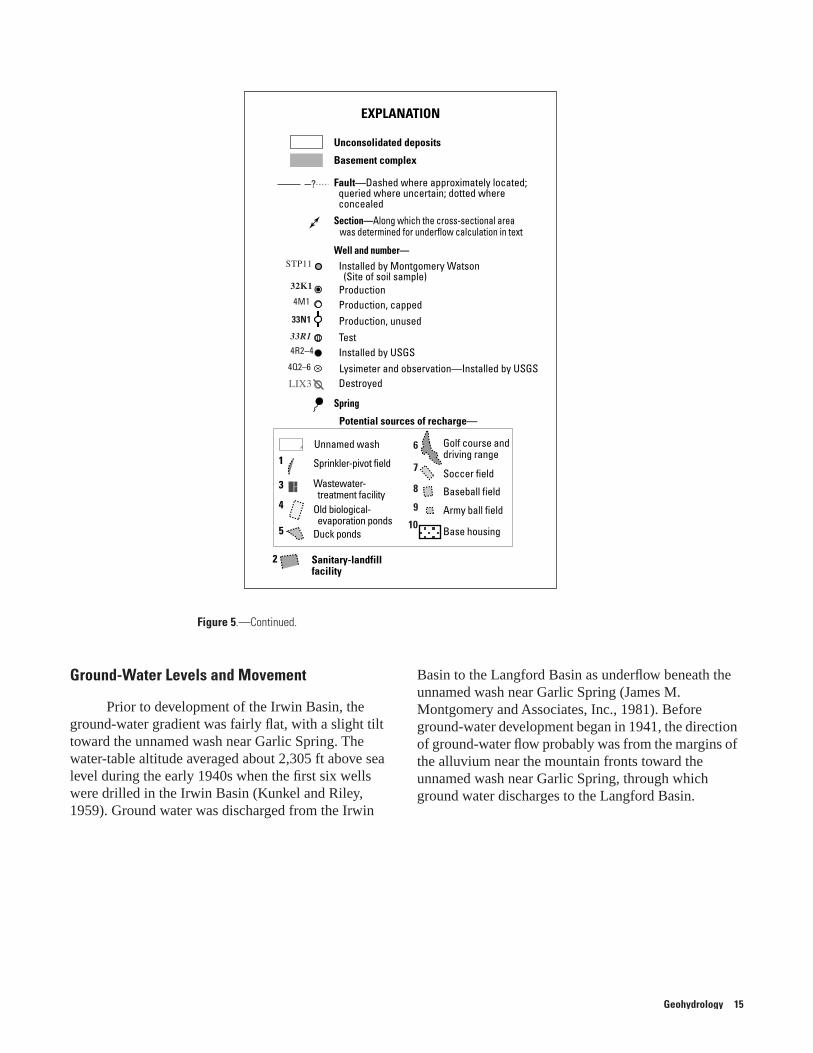
Ground-water pumpage in the Irwin Basin began in 1941 with the drilling and installation of the first two wells for water supply at Camp Irwin. From 1941 to 1966, all the water used at the base was supplied from wells in the Irwin Basin. In 1967, the U.S. Army began pumping ground water from the Bicycle Basin to the north of the Irwin Basin, and in 1992, they began pumping ground water from the Langford Basin to the southeast of the Irwin Basin (fig. 1). Most of the water pumped from the Bicycle and the Langford Basins was piped to the Irwin Basin. Pumpage from 1941 to 1999 is summarized in table 2 for these three basins. The location of production and observation wells in the Irwin Basin is shown in figure 5. Total ground-water pumpage from the three basins ranged from about 30 acre-ft in 1941 to more than 3,000 acre-ft in 1999, with as much as 1,927 acre-ft (the largest volume) being pumped from the Irwin Basin in 1987 (table 2).
Most of the water that has not been consumed in the Irwin Basin has been discharged to the wastewater-collection system and treatment facility in the basin. From 1941 to 1955, wastewater was collected in biological-evaporation ponds in the northeastern part of the basin (shown as old biological-evaporation ponds in figure 5), and from 1955 until present (1999), it was collected and treated at the wastewater-treatment facility in the southeastern part of the basin. Densmore and Londquist (1997) estimated that a maximum of 70 percent of total pumpage and a minimum of 58 percent of total pumpage was collected at the biological-evaporation ponds during 1941-55 and then at the wastewater-treatment facility between 1955 and 1993 (table 3); these values also were assumed valid for the recent period 1994 through 1999 (table 3).
The percolation (infiltration) of wastewater to the water table is the largest source of ground-water recharge in the Irwin Basin (Densmore and Londquist, 1997). Between 1941 and 1955, untreated wastewater
was disposed in the old biological-evaporation ponds, but since 1955 it has been treated and disposed in ponds at the wastewater-treatment facility in the southeastern part of the basin (fig. 5). Some of the treated wastewater is diverted from the wastewater-treatment facility ponds to irrigate the base golf course/driving range and sprinkler-pivot field, and to infiltrate the subsurface sediments beneath two overflow ponds, referred to as duck ponds (fig. 5). The golf course and driving range were irrigated from 1955 to 1971 and from 1981 to 1999. Although part of the golf course and driving range lies outside the basin boundary, the water used to irrigate these areas is assumed to recharge the ground-water system. In 1986, a sprinkler-pivot field was added in the southeastern part of the basin to provide additional disposal. Since 1996, when the first phase of this study showed that ground-water degradation occurred due to leaching evaporite deposits beneath the sprinkler-pivot field, all disposal of wastewater through the sprinkler-pivot field has ceased (Kevin Maggs, Fort Irwin National Training Center, oral commun., 2000). The duck ponds are filled intermittently, depending on demand for the treated wastewater.
Another source of recharge not present before development of the base is the infiltration of water used to irrigate lawns and playing fields that is not consumed by the plants. About 14 acres of lawn was watered during the mid-1960s to the early 1980s; this includes lawns at the base housing and at an Army ball field. In 1983, the housing area increased to about 25 acres. During 1984–85, an additional 8 acres of irrigated area (soccer field and a baseball field complex) was added adjacent to the base housing in the western part of the basin (fig. 2). By the mid-1980’s, the total irrigated area was 33 acres. The potential artificial recharge from irrigation-return water (applied irrigation water in excess of that used by the plants) for these 33 acres was about 90 acre-ft/yr before the early-1980s, and about 210 acre-ft/yr from the early 1980s to present (1999) (Densmore and Londquist, 1997).
Geohydrology 13
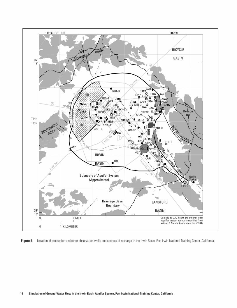
Figure 5. Location of production and other observation wells and sources of recharge in the Irwin Basin, Fort Irwin National Training Center, California.
Barstow
Rd
Irwin
Rd
N. Loop Rd
Langford LakeRd
BICYCLE
LAKE FAULT
Drainage BasinBoundary
Boundary of Aquifer System(Approximate)
LANGFORD
BASIN
IRWIN
BASIN
BICYCLE
BASINNORTHWEST
RIDGE
NORTHWESTRIDGE
SOUTHWEST
RIDGE
BeaconHill
BeaconHill
GarlicSpring
S. Loop Rd
36
1 6
312
6
1
0 1 MILE
OldOld
NewNew
6P1
33
5
4
97
8
1032B1–3
32F2–332F1
32H1
32M1 32L132K1
32P131K1
32J1
32N1–35D1 32P2–6
32Q332Q2
32Q1
33N1
5G2
32K3–6
5G1
33F133B1
33H133G2
33G333G4
33G1 33J1
34D1
33H233H3
34M1
33Q1
4G14K1
33R1
33A1
33E2–3
33J234M2
4B1-3
4D1–3
4C1–34B4–8
STP3R
STP11STP9
STP8
STP7
4M1
4Q2-64Q2–6
8B110E1-310E1–3
4K2-44K2–4
4Q1
9B110D110D1
LIX3
4B1-34B1–3
GARLICSPRING
FAULT
116°39'116°43'
35°17'
35°13'
T14NT13N
R2E R3E
Geology by J. C. Yount and others (1994)Aquifer system boundary modified fromWilson F. So and Associates, Inc. (1989)
1 KILOMETER0
14 Simulation of Ground-Water Flow in the Irwin Basin Aquifer System, Fort Irwin National Training Center, California
Ground-Water Levels and Movement
Prior to development of the Irwin Basin, the ground-water gradient was fairly flat, with a slight tilt toward the unnamed wash near Garlic Spring. The water-table altitude averaged about 2,305 ft above sea level during the early 1940s when the first six wells were drilled in the Irwin Basin (Kunkel and Riley, 1959). Ground water was discharged from the Irwin
Basin to the Langford Basin as underflow beneath the unnamed wash near Garlic Spring (James M. Montgomery and Associates, Inc., 1981). Before ground-water development began in 1941, the direction of ground-water flow probably was from the margins of the alluvium near the mountain fronts toward the unnamed wash near Garlic Spring, through which ground water discharges to the Langford Basin.
Figure 5.—Continued.
Unnamed wash
LIX3
Potential sources of recharge—
Sanitary-landfillfacility
EXPLANATION
Unconsolidated deposits
Basement complex
Fault—Dashed where approximately located;queried where uncertain; dotted whereconcealed
Installed by Montgomery Watson(Site of soil sample)
ProductionProduction, cappedProduction, unusedTestInstalled by USGS
Destroyed
Golf course anddriving range
Soccer field
Baseball field
Army ball field
Base housing
Sprinkler-pivot field
Wastewater-treatment facility
Old biological-evaporation ponds
Duck ponds
1
2
3
4
5
Section—Along which the cross-sectional areawas determined for underflow calculation in text
Well and number—
Spring
STP11
32K1
4M1
33N1
33R1
4R2–4
6
7
8
9
10
4Q2–6 Lysimeter and observation—Installed by USGS
?
Geohydrology 15
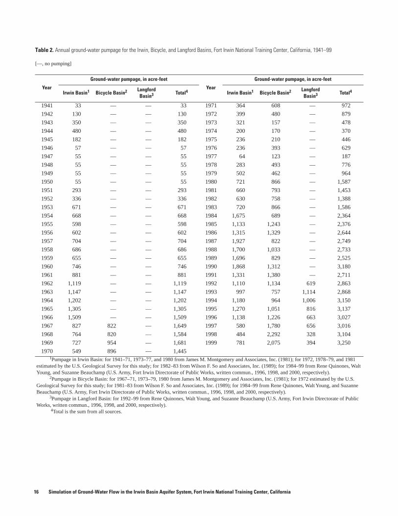
Table 2. Annual ground-water pumpage for the Irwin, Bicycle, and Langford Basins, Fort Irwin National Training Center, California, 1941–99
[—, no pumping]
Year
Ground-water pumpage, in acre-feet
Year
Ground-water pumpage, in acre-feet
Irwin Basin1 Bicycle Basin2 Langford Basin3 Total4 Irwin Basin1 Bicycle Basin2 Langford
Basin3 Total4
1941 33 — — 33 1971 364 608 — 972
1942 130 — — 130 1972 399 480 — 879
1943 350 — — 350 1973 321 157 — 478
1944 480 — — 480 1974 200 170 — 370
1945 182 — — 182 1975 236 210 — 446
1946 57 — — 57 1976 236 393 — 629
1947 55 — — 55 1977 64 123 — 187
1948 55 — — 55 1978 283 493 — 776
1949 55 — — 55 1979 502 462 — 964
1950 55 — — 55 1980 721 866 — 1,587
1951 293 — — 293 1981 660 793 — 1,453
1952 336 — — 336 1982 630 758 — 1,388
1953 671 — — 671 1983 720 866 — 1,586
1954 668 — — 668 1984 1,675 689 — 2,364
1955 598 — — 598 1985 1,133 1,243 — 2,376
1956 602 — — 602 1986 1,315 1,329 — 2,644
1957 704 — — 704 1987 1,927 822 — 2,749
1958 686 — — 686 1988 1,700 1,033 — 2,733
1959 655 — — 655 1989 1,696 829 — 2,525
1960 746 — — 746 1990 1,868 1,312 — 3,180
1961 881 — — 881 1991 1,331 1,380 — 2,711
1962 1,119 — — 1,119 1992 1,110 1,134 619 2,863
1963 1,147 — — 1,147 1993 997 757 1,114 2,868
1964 1,202 — — 1,202 1994 1,180 964 1,006 3,150
1965 1,305 — — 1,305 1995 1,270 1,051 816 3,137
1966 1,509 — — 1,509 1996 1,138 1,226 663 3,027
1967 827 822 — 1,649 1997 580 1,780 656 3,016
1968 764 820 — 1,584 1998 484 2,292 328 3,104
1969 727 954 — 1,681 1999 781 2,075 394 3,250
1970 549 896 — 1,4451Pumpage in Irwin Basin: for 1941–71, 1973–77, and 1980 from James M. Montgomery and Associates, Inc. (1981); for 1972, 1978–79, and 1981
estimated by the U.S. Geological Survey for this study; for 1982–83 from Wilson F. So and Associates, Inc. (1989); for 1984–99 from Rene Quinones, Walt Young, and Suzanne Beauchamp (U.S. Army, Fort Irwin Directorate of Public Works, written commun., 1996, 1998, and 2000, respectively).
2Pumpage in Bicycle Basin: for 1967–71, 1973–79, 1980 from James M. Montgomery and Associates, Inc. (1981); for 1972 estimated by the U.S. Geological Survey for this study; for 1981–83 from Wilson F. So and Associates, Inc. (1989); for 1984–99 from Rene Quinones, Walt Young, and Suzanne Beauchamp (U.S. Army, Fort Irwin Directorate of Public Works, written commun., 1996, 1998, and 2000, respectively).
3Pumpage in Langford Basin: for 1992–99 from Rene Quinones, Walt Young, and Suzanne Beauchamp (U.S. Army, Fort Irwin Directorate of Public Works, written commun., 1996, 1998, and 2000, respectively).
4Total is the sum from all sources.
16 Simulation of Ground-Water Flow in the Irwin Basin Aquifer System, Fort Irwin National Training Center, California
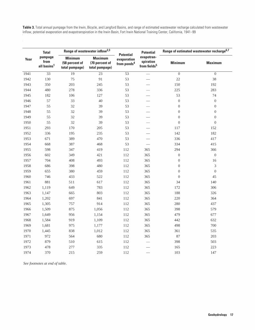
[All values are reported in acre-feet. Recharge estimates modified from Densmore and Londquist (1997, table 3). —, no data]
Table 3. Total annual pumpage from the Irwin, Bicycle, and Langford Basins, and range of estimated wastewater recharge calculated from wastewater inflow, potential evaporation and evapotranspiration in the Irwin Basin, Fort Irwin National Training Center, California, 1941–99
Table 3. Total annual pumpage from the Irwin, Bicycle, and Langford Basins, and range of estimated wastewater recharge calculated from wastewater inflow, potential evaporation and evapotranspiration in the Irwin Basin, Fort Irwin National Training Center, California, 1941–99
Year
Totalpumpage
fromall basins1
Range of wastewater inflow2,3
Potential evaporationfrom ponds4
Potential evapotran-spiration
from fields5
Range of estimated wastewater recharge6,7
Minimum(58 percent of
total pumpage)
Maximum(70 percent of
total pumpage)Minimum Maximum
1941 33 19 23 53 — 0 0
1942 130 75 91 53 — 22 38
1943 350 203 245 53 — 150 192
1944 480 278 336 53 — 225 283
1945 182 106 127 53 — 53 74
1946 57 33 40 53 — 0 0
1947 55 32 39 53 — 0 0
1948 55 32 39 53 — 0 0
1949 55 32 39 53 — 0 0
1950 55 32 39 53 — 0 0
1951 293 170 205 53 — 117 152
1952 336 195 235 53 — 142 182
1953 671 389 470 53 — 336 417
1954 668 387 468 53 — 334 415
1955 598 347 419 112 365 294 366
1956 602 349 421 112 365 0 0
1957 704 408 493 112 365 0 16
1958 686 398 480 112 365 0 3
1959 655 380 459 112 365 0 0
1960 746 433 522 112 365 0 45
1961 881 511 617 112 365 34 140
1962 1,119 649 783 112 365 172 306
1963 1,147 665 803 112 365 188 326
1964 1,202 697 841 112 365 220 364
1965 1,305 757 914 112 365 280 437
1966 1,509 875 1,056 112 365 398 579
1967 1,649 956 1,154 112 365 479 677
1968 1,584 919 1,109 112 365 442 632
1969 1,681 975 1,177 112 365 498 700
1970 1,445 838 1,012 112 365 361 535
1971 972 564 680 112 365 87 203
1972 879 510 615 112 — 398 503
1973 478 277 335 112 — 165 223
1974 370 215 259 112 — 103 147
See footnotes at end of table.
Geohydrology 17
1975 446 259 312 112 — 147 200
1976 629 365 440 112 — 253 328
1977 187 108 131 112 — 0 19
1978 776 450 543 112 — 338 431
1979 964 559 675 112 — 447 563
1980 1,587 920 1,111 112 — 808 999
1981 1,453 843 1,017 112 365 366 540
1982 1,388 805 972 112 365 328 495
1983 1,586 920 1,110 112 365 443 633
1984 2,364 1,371 1,655 112 365 894 1,178
1985 2,376 1,378 1,663 112 365 901 1,186
1986 2,644 1,534 1,851 310 430 794 1,111
1987 2,749 1,594 1,924 310 430 854 1,184
1988 2,733 1,585 1,913 310 430 845 1,173
1989 2,525 1,465 1,768 310 430 725 1,028
1990 3,180 1,844 2,226 310 430 1,104 1,486
1991 2,711 1,572 1,898 310 430 832 1,158
1992 2,863 1,661 2,004 310 430 921 1,264
1993 2,868 1,663 2,008 310 430 923 1,268
1994 3,150 1,827 2,205 310 430 1,087 1,465
1995 3,137 1,819 2,196 310 430 1,079 1,456
1996 3,027 1,756 2,119 310 430 1,016 1,379
1997 3,016 1,749 2,111 310 365 1,074 1,436
1998 3,104 1,800 2,173 310 365 1,125 1,498
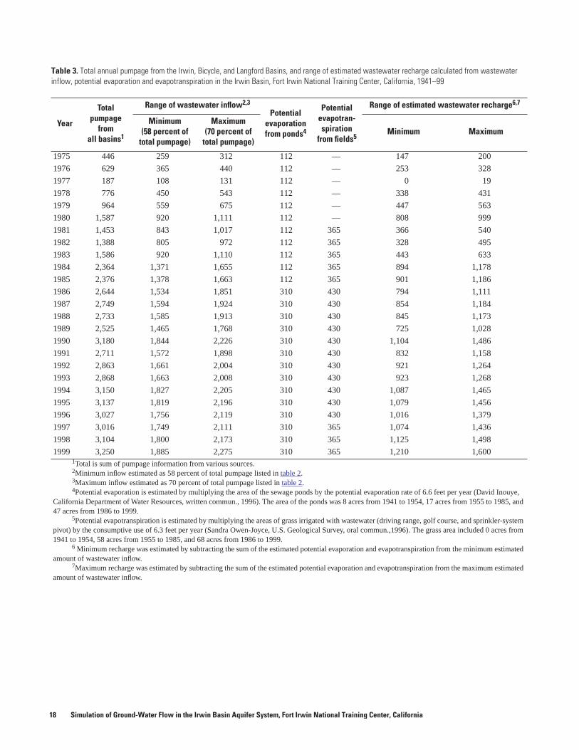
1999 3,250 1,885 2,275 310 365 1,210 1,6001Total is sum of pumpage information from various sources.2Minimum inflow estimated as 58 percent of total pumpage listed in table 2.3Maximum inflow estimated as 70 percent of total pumpage listed in table 2.4Potential evaporation is estimated by multiplying the area of the sewage ponds by the potential evaporation rate of 6.6 feet per year (David Inouye,
California Department of Water Resources, written commun., 1996). The area of the ponds was 8 acres from 1941 to 1954, 17 acres from 1955 to 1985, and 47 acres from 1986 to 1999.
5Potential evapotranspiration is estimated by multiplying the areas of grass irrigated with wastewater (driving range, golf course, and sprinkler-system pivot) by the consumptive use of 6.3 feet per year (Sandra Owen-Joyce, U.S. Geological Survey, oral commun.,1996). The grass area included 0 acres from 1941 to 1954, 58 acres from 1955 to 1985, and 68 acres from 1986 to 1999.
6 Minimum recharge was estimated by subtracting the sum of the estimated potential evaporation and evapotranspiration from the minimum estimated amount of wastewater inflow.
7Maximum recharge was estimated by subtracting the sum of the estimated potential evaporation and evapotranspiration from the maximum estimated amount of wastewater inflow.
Table 3. Total annual pumpage from the Irwin, Bicycle, and Langford Basins, and range of estimated wastewater recharge calculated from wastewater inflow, potential evaporation and evapotranspiration in the Irwin Basin, Fort Irwin National Training Center, California, 1941–99
Year
Totalpumpage
fromall basins1
Range of wastewater inflow2,3
Potential evaporationfrom ponds4
Potential evapotran-spiration
from fields5
Range of estimated wastewater recharge6,7
Minimum(58 percent of
total pumpage)
Maximum(70 percent of
total pumpage)Minimum Maximum
18 Simulation of Ground-Water Flow in the Irwin Basin Aquifer System, Fort Irwin National Training Center, California
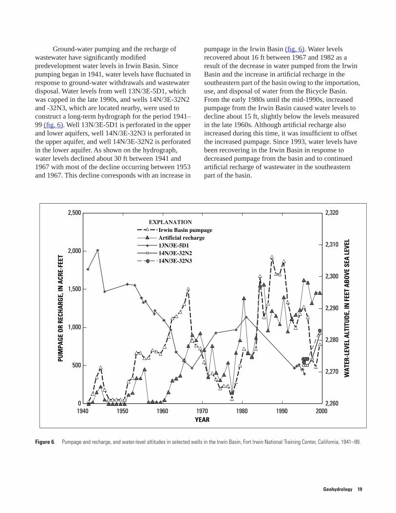
Ground-water pumping and the recharge of wastewater have significantly modified predevelopment water levels in Irwin Basin. Since pumping began in 1941, water levels have fluctuated in response to ground-water withdrawals and wastewater disposal. Water levels from well 13N/3E-5D1, which was capped in the late 1990s, and wells 14N/3E-32N2 and -32N3, which are located nearby, were used to construct a long-term hydrograph for the period 1941–99 (fig. 6). Well 13N/3E-5D1 is perforated in the upper and lower aquifers, well 14N/3E-32N3 is perforated in the upper aquifer, and well 14N/3E-32N2 is perforated in the lower aquifer. As shown on the hydrograph, water levels declined about 30 ft between 1941 and 1967 with most of the decline occurring between 1953 and 1967. This decline corresponds with an increase in
pumpage in the Irwin Basin (fig. 6). Water levels recovered about 16 ft between 1967 and 1982 as a result of the decrease in water pumped from the Irwin Basin and the increase in artificial recharge in the southeastern part of the basin owing to the importation, use, and disposal of water from the Bicycle Basin. From the early 1980s until the mid-1990s, increased pumpage from the Irwin Basin caused water levels to decline about 15 ft, slightly below the levels measured in the late 1960s. Although artificial recharge also increased during this time, it was insufficient to offset the increased pumpage. Since 1993, water levels have been recovering in the Irwin Basin in response to decreased pumpage from the basin and to continued artificial recharge of wastewater in the southeastern part of the basin.
Figure 6. Pumpage and recharge, and water-level altitudes in selected wells in the Irwin Basin, Fort Irwin National Training Center, California, 1941–99.
1940 1950 1960 1970 1980 1990 2000YEAR
PUM
PAG
EO
RRE
CHA
RGE,
INA
CRE-
FEET
WA
TER-
LEVE
LA
LTIT
UD
E,IN
FEET
AB
OVE
SEA
LEVE
L
Irwin Basin pumpageArtificial recharge13N/3E-5D114N/3E-32N214N/3E-32N3
0
500
1,000
1,500
2,000
2,500
2,260
2,270
2,280
2,290
2,300
2,310
2,320EXPLANATION
Geohydrology 19
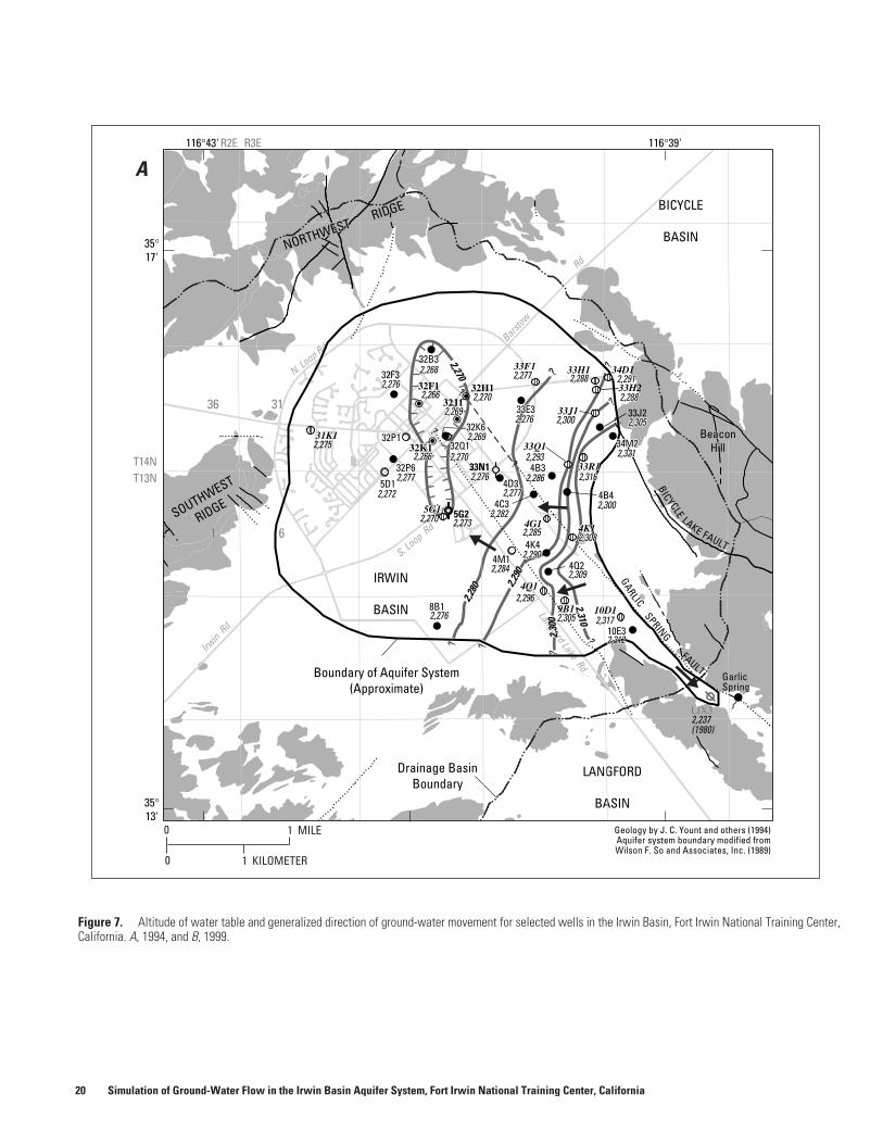
Figure 7. Altitude of water table and generalized direction of ground-water movement for selected wells in the Irwin Basin, Fort Irwin National Training Center, California. A, 1994, and B, 1999.
Barstow
Rd
Irwin
Rd
N. Loop RdLangford Lake
Rd
BICYCLE
LAKE FAULT
Drainage BasinBoundary
Boundary of Aquifer System(Approximate)
LANGFORD
BASIN
IRWIN
BASIN
BICYCLE
BASINNORTHWEST
RIDGE
NORTHWESTRIDGE
SOUTHWEST
RIDGE
BeaconHill
BeaconHill
GarlicSpring
S. Loop Rd
36
1 6
31
0
1 KILOMETER
1 MILE
2,268
2,277 2,2762,276
2,2772,277
2,2822,2822,300
2,3082,3082,285
2,2902,290
2,296
2,3052,305
2,3122,312
2,3172,317
2,293
2,2772,269
2,2882,276
?
2,2952,2952,2862,286
0
32B332F3
32F1 32H1
32P131K1
5D1
32P632P6
32Q132Q1
33N1
5G2
32K632K6
33F1 33H1
33J1
34D1
33H2
33Q1
4G1 4K1
33R1
33E333E3 33J2
34M234M2
4D3
4C34B4
4M14M14Q2
8B1
10E310E3
4K44K4
4Q1
9B1 10D110D1
4B3
GARLICSPRING
FAULT
116°39'116°43'
35°17'
35°13'
T14NT13N
R2E R3E
A
2,270
2,280 2,2
90
2,30
0
2,310
?
?
??
?
?
?
?
2,276
2,237(1980)
2,272
2,275
2,266
2,270 2,273
2,270
2,2842,284 2,309
4B3?
?
?2,3212,321
2,3052,305
2,2882,288
2,2912,2912,2882,288
2,3002,300
2,3162,316
2,2762,276
2,2772,277
32K132K12,2702,2702,2662,266
5G15G1
2,2692,26932J1
Geology by J. C. Yount and others (1994)Aquifer system boundary modified fromWilson F. So and Associates, Inc. (1989)
LIX3
20 Simulation of Ground-Water Flow in the Irwin Basin Aquifer System, Fort Irwin National Training Center, California
Water-level measurements from the shallowest well at multiple-well monitoring sites and from test wells, which generally are perforated near the water table, were used to develop 1994 and 1999 water-table maps shown in figure 7. The 1994 water-table map shows that pumpage has created a water-table depression (or pumping depression) in the central part of the basin (fig. 7A). The general direction of ground-water movement throughout most of the basin was from the margin of the basin toward the pumping depression. A ground-water mound and a ground-water divide have formed as a result of wastewater disposal in the southeastern part of the basin, where the water-table altitude was more than 2,310 ft above sea level (fig. 7A). The 1999 water-table map (fig. 7B) shows that the pumping depression remained in the central part of the basin beneath the well field; however, the altitude of the water table had risen about 8 ft from 2,269 ft above sea level in well 14N/3E-32K6 in 1994 to 2,277 ft in 1999. The direction of ground-water movement throughout most of the basin is still toward the pumping depression (fig. 7B). The ground-water mound and divide also are still present in the
southeastern part of the basin (fig. 7B). The ground-water table has risen about 7 ft from 2,312 ft above sea level in well 13N/3E-10E3 in 1994 to 2,319 ft in 1999. Water from the mound continues to flow northwestward toward the ground-water depression in the central part of the basin and southeastward toward the unnamed wash near Garlic Spring.
Water-level data from multiple-well monitoring sites indicate that the hydraulic head (or water level) varies slightly with depth (Densmore and Londquist, 1997; Appendix B). Generally, the hydraulic head is higher in wells perforated in the upper aquifer than in wells perforated in the lower aquifer. This difference in hydraulic head indicates the potential for downward vertical flow. The largest differences in hydraulic head are about 3 ft at wells 13N/3E-10E1-3 in the southeastern part of the basin and about 8 ft at wells 14N/3E-32N1-3 and 32P2-6 in the west-central part of the basin (Densmore and Londquist, 1997). This difference in hydraulic head probably is due to wastewater disposal and irrigation return, respectively, near these sites (fig. 5).
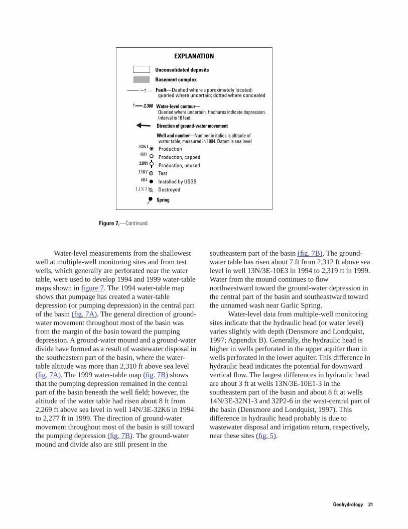
Figure 7,—Continued.
? 2,300
EXPLANATION
Unconsolidated deposits
Basement complex
Fault—Dashed where approximately located;queried where uncertain; dotted where concealed
Production
Production, capped
Production, unusedTest
Installed by USGSDestroyed
Well and number—Number in italics is altitude ofwater table, measured in 1994. Datum is sea level
Water-level contour—Queried where uncertain. Hachures indicate depression.Interval is 10 feet
Direction of ground-water movement
Spring
?
32K1
4M1
33N1
33R1
4B4
LIX3
Geohydrology 21
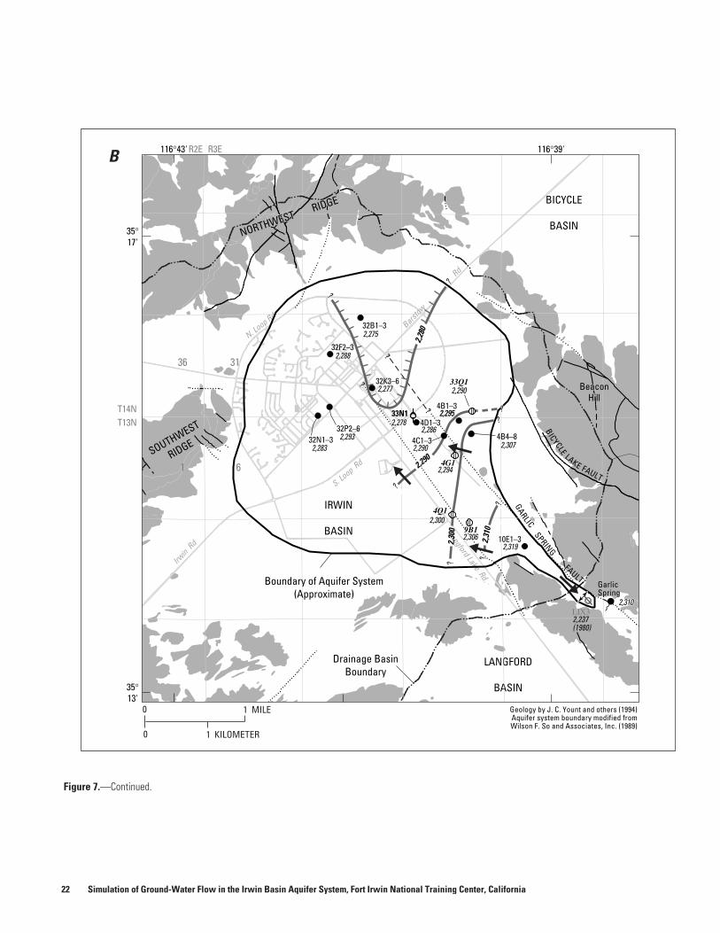
Figure 7.—Continued.
Barstow
Rd
Irwin
Rd
N. Loop Rd
Langford LakeRd
Unnamed wash
BICYCLE
LAKE FAULT
Drainage BasinBoundary
Boundary of Aquifer System(Approximate)
LANGFORD
BASIN
IRWIN
BASIN
BICYCLE
BASINNORTHWEST
RIDGE
NORTHWESTRIDGE
SOUTHWEST
RIDGE
BeaconHill
BeaconHill
GarlicSpring
S. Loop Rd
36
1 6
31
0
1 KILOMETER
1 MILE
2,275
2,293
2,2782,2782,2862,286
2,2902,290 2,307
2,294
2,300
2,3102,310
2,3062,3062,3192,319
2,290
2,283
2,2772,277
2,2882,288
?
?
??
?
?
??
?
?2,
280
2,2902,290
2,30
0
2,31
0
2,2952,2952,295
0
32B1–3
32F2–3
32N1–332P2–6
33N1
32K3–6 33Q1
4G1
4D1–34D1–3
4C1–3 4B4–8
10E1-310E1–3
4Q1
9B19B1
4B1-3
GARLICSPRING
FAULT
116°39'116°43'
35°17'
35°13'
T14NT13N
R2E R3EB
4B1–3
?
?
?
Geology by J. C. Yount and others (1994)Aquifer system boundary modified fromWilson F. So and Associates, Inc. (1989)
LIX32,237(1980)
22 Simulation of Ground-Water Flow in the Irwin Basin Aquifer System, Fort Irwin National Training Center, California
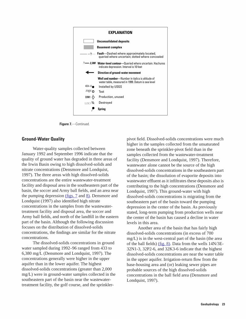
Ground-Water Quality
Water-quality samples collected between January 1992 and September 1996 indicate that the quality of ground water has degraded in three areas of the Irwin Basin owing to high dissolved-solids and nitrate concentrations (Densmore and Londquist, 1997). The three areas with high dissolved-solids concentrations are the entire wastewater-treatment facility and disposal area in the southeastern part of the basin, the soccer and Army ball fields, and an area near the pumping depression (figs. 7 and 8). Densmore and Londquist (1997) also identified high nitrate concentrations in the samples from the wastewater-treatment facility and disposal area, the soccer and Army ball fields, and north of the landfill in the eastern part of the basin. Although the following discussion focuses on the distribution of dissolved-solids concentrations, the findings are similar for the nitrate concentrations.
The dissolved-solids concentrations in ground water sampled during 1992–96 ranged from 433 to 6,380 mg/L (Densmore and Londquist, 1997). The concentrations generally were higher in the upper aquifer than in the lower aquifer. The highest dissolved-solids concentrations (greater than 2,000 mg/L) were in ground-water samples collected in the southeastern part of the basin near the wastewater-treatment facility, the golf course, and the sprinkler-
pivot field. Dissolved-solids concentrations were much higher in the samples collected from the unsaturated zone beneath the sprinkler-pivot field than in the samples collected from the wastewater-treatment facility (Densmore and Londquist, 1997). Therefore, wastewater alone cannot be the source of the high dissolved-solids concentrations in the southeastern part of the basin; the dissolution of evaporite deposits into wastewater effluent as it infiltrates these deposits also is contributing to the high concentrations (Densmore and Londquist, 1997). This ground-water with high dissolved-solids concentrations is migrating from the southeastern part of the basin toward the pumping depression in the center of the basin. As previously stated, long-term pumping from production wells near the center of the basin has caused a decline in water levels in this area.
Another area of the basin that has fairly high dissolved-solids concentrations (in excess of 700 mg/L) is in the west-central part of the basin (the area of the ball fields) (fig. 8). Data from the wells 14N/3E-32N1-3, 32P2-6, and 32K3-6 indicate that the highest dissolved-solids concentrations are near the water table in the upper aquifer. Irrigation-return flow from the base-housing area and (or) leaking sewer pipes are probable sources of the high dissolved-solids concentrations in the ball field area (Densmore and Londquist, 1997).
Figure 7.—Continued.
EXPLANATION
Production, unused
Destroyed
TestInstalled by USGS
33N1
33Q1
4B4–8
? 2,300
Unconsolidated deposits
Basement complex
Fault—Dashed where approximately located;queried where uncertain; dotted where concealed
Well and number—Number in italics is altitude ofwater table, measured in 1999. Datum is sea level
Water-level contour—Queried where uncertain. Hachuresindicate depression. Interval is 10 feet
Direction of ground-water movement
Spring
LIX3
Geohydrology 23
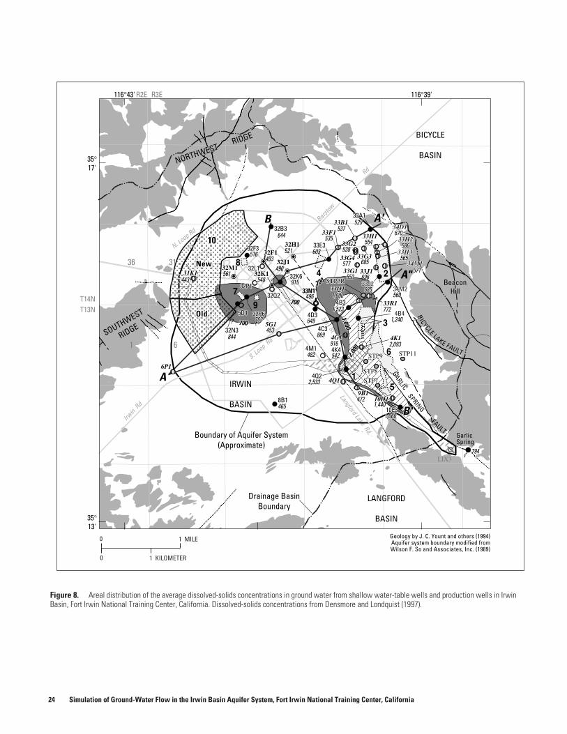
Figure 8. Areal distribution of the average dissolved-solids concentrations in ground water from shallow water-table wells and production wells in Irwin Basin, Fort Irwin National Training Center, California. Dissolved-solids concentrations from Densmore and Londquist (1997).
Barstow
Rd
Irwin
Rd
N. Loop RdLangford Lake
Rd
5thSt
S. Loop Rd
BICYCLE LAKE FAULT
Drainage BasinBoundary
Boundary of Aquifer System(Approximate)
LANGFORD
BASIN
IRWIN
BASIN
BICYCLE
BASINNORTHWEST
RIDGE
NORTHWESTRIDGE
SOUTHWEST
RIDGESOUTHWEST
RIDGE
BeaconHill
BeaconHill
GarlicSpring
?
?
36
1 6
31
?
? ?
1010
NewNew
OldOld
2,000
2,000
1,0001,000
B A'
A
A"
B'B'
GARLICSPRING
FAULT
844
561443443
763
453
465
482 542
794
516493
644
521
915
603
535537
529529
670670
586586
571571
565565
490
548
1,0001,000
1,5231,523
1,240772
685
763
685
685
554
696553553
577
538
560560
916869
649
496
472472
1,0601,060
1,4401,440
2,0932,093
2,5332,533
700700
700700
700700
32B1-3
32F3
32L132K6
33E3
32P132Q2
5D1 32P6
32N3
8B1
5G1
31K132M132M1
32K132K1
32F132F1
32J132J1
32H132H1
33A1
33N1
33B1
33F133H1
33G2
33G333G4
33G1 33J1
33Q1
33R1
STP3R
4D3
4C3
4K44M1
4G1
4B3
4Q24Q1
9B110D1
10E3
STP7
STP8
STP9 STP11
4K1
4B4
34M233J2
34M1
33H3
33H2
34D1
6P1
32B3
32F3
32L132K6
33E3
32P132Q2
5D1 32P6
32N3
8B1
5G1
31K1
33A1
33N1
33B1
33F133H1
33G2
33G333G4
33G1 33J1
33Q1
33R1
STP3R
4D3
4C3
4K44M1
4G1
4B3
4Q24Q1
9B110D1
10E3
STP7
STP8
STP9 STP11
4K1
4B4
34M233J2
34M1
33H3
33H2
34D1
6P1
0
0
1 KILOMETER
1 MILE
116°39'116°43'
35°17'
35°13'
T14NT13N
R2E R3E
Geology by J. C. Yount and others (1994)Aquifer system boundary modified fromWilson F. So and Associates, Inc. (1989)
LIX3
24 Simulation of Ground-Water Flow in the Irwin Basin Aquifer System, Fort Irwin National Training Center, California
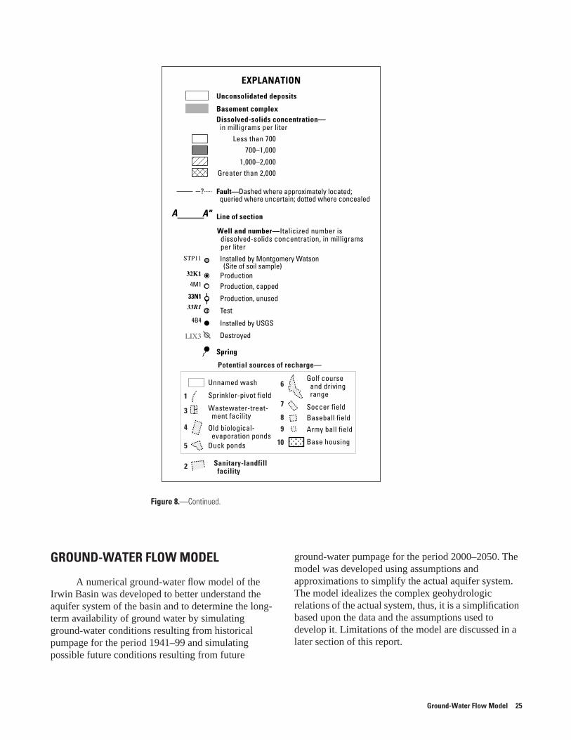
GROUND-WATER FLOW MODEL
A numerical ground-water flow model of the Irwin Basin was developed to better understand the aquifer system of the basin and to determine the long-term availability of ground water by simulating ground-water conditions resulting from historical pumpage for the period 1941–99 and simulating possible future conditions resulting from future
ground-water pumpage for the period 2000–2050. The model was developed using assumptions and approximations to simplify the actual aquifer system. The model idealizes the complex geohydrologic relations of the actual system, thus, it is a simplification based upon the data and the assumptions used to develop it. Limitations of the model are discussed in a later section of this report.
Figure 8.—Continued.
LIX3
Unnamed wash
Sprinkler-pivot field
Wastewater-treat-ment facility
Old biological-evaporation ponds
Duck ponds
Golf courseand drivingrange
Soccer fieldBaseball fieldArmy ball field
Base housing
Sanitary-landfillfacility
Potential sources of recharge—
1
6
7
8
9
10
3
4
5
2
Well and number—Italicized number isdissolved-solids concentration, in milligramsper liter
Dissolved-solids concentration—in milligrams per liter
Less than 700700–1,000
1,000–2,000Greater than 2,000
Line of section
Spring
A A"
Fault—Dashed where approximately located;queried where uncertain; dotted where concealed
Unconsolidated deposits
EXPLANATION
Installed by Montgomery Watson(Site of soil sample)
ProductionProduction, capped
Production, unused
Test
Installed by USGS
Destroyed
33R1
33N1
4M1
4B4
32K1
STP11
Basement complex
?
Ground-Water Flow Model 25
The USGS Modular Three-Dimensional Finite-Difference Ground-Water Flow Model (MODFLOW) developed by McDonald and Harbaugh (1988) was used to simulate flow in the Irwin Basin. Although the model only is an approximation of the actual ground-water flow system, the model can be used to determine gaps and potential anomalies in data and in understanding the aquifer system. The ground-water flow system in the Irwin Basin was numerically defined by discretizing the aquifer system into a finite-difference grid, determining the boundary conditions for the aquifers, estimating the rates and distribution of recharge and discharge, and estimating the aquifer properties within the model. The accuracy of these input data, in part determines the accuracy of the model.
To simulate historical conditions, steady-state (predevelopment) and transient-state (postdevelopment) models were formulated and calibrated. Results of the steady-state simulation were used as initial conditions for the transient-state model.
Model Grid
The model is represented by a rectangular finite-difference grid discretized into rows and columns that form model cells where the ground-water flow equation is solved numerically at nodes at the center of each cell (McDonald and Harbaugh, 1988). Figure 9 shows the area of the local model grid for the Irwin Basin and the regional model grid for the Fort Irwin NTC. The regional grid consists of 152 rows and 125 columns. The origin of the regional grid (that is, the upper left corner of the grid; row 1, column 1) is at an easting of 2,373,237 ft and a northing of 669,380 ft in zone 5 of the California State plane coordinate system. The size of the regional grid is large enough to include the Irwin, Bicycle, and Langford Basins, all of which supply water to Fort Irwin. The regional grid was designed to include these three basins so that as future models of the Langford and Bicycle Basins are completed, they can be incorporated into one large model that can be used to help the Fort Irwin NTC manage water resources on a regional basis. The model
cells are 500 ft by 500 ft along the x and y axis. The local grid for the Irwin Basin is within the regional grid. The same grid and cell sizes are used for the local model grid of the Irwin Basin, but only cells in rows 1 to 80 and columns 1 to 64 represent the local model grid for the Irwin Basin (fig. 9). For ease of viewing the figures showing model parameters, inactive cells in rows 1 to 35 and columns 1 to 24 are not shown: only cells in rows 36 to 80 and columns 25 to 64, which contain the Irwin Basin, are shown.
The aquifer system was vertically discretized into two horizontal layers of cells (figs. 10 and 11). Layer 1 represents the unconfined upper aquifer and has a variable thickness ranging from about 1 to 100 ft, depending on the saturated thickness of the aquifer materials (fig. 11). The top altitude of layer 1 represents the water table. The bottom altitude of layer 1 (the bottom of the upper aquifer) is 2,200 ft above sea level throughout most of the basin and consists of primarily younger alluvium. In the southeastern part of the basin, the bottom of layer 1 is defined as the top of the lacustrine deposits of the lower aquifer. Layer 2 represents the confined lower aquifer, underlies layer 1 throughout most of the model area, and has a variable thickness ranging from about 1 to 600 ft depending on the altitude of the underlying basement complex (fig. 11). The top of layer 2, which is the bottom of layer 1, is 2,200 ft above sea level where it underlies layer 1, and the bottom of layer 2 is the altitude of the underlying basement complex. Layer 1 and layer 2 contain 784 and 538 active cells, respectively. Layer 2 has fewer active cells than layer 1 because some of the cells, along the outer edge of the basin and in the mouth of the wash that passes Garlic Spring, bounded the Garlic Spring and unnamed faults, are in areas of the basement complex that are higher in elevation than that of the top of layer 2 (2,200 ft above sea level); thus, there is no layer 2 in these areas.
The MODFLOW packages used in this model include Basic (BAS), Block-Centered Flow (BCF), Well (WEL), General-Head Boundary (GHB), Horizontal-Flow-Barrier (HFB), and Strongly Implicit Procedure (SIP) [BAS, BCF, WEL, GHB, and SIP (McDonald and Harbaugh, 1988), and HFB (Hsieh and Freckleton, 1993)].
26 Simulation of Ground-Water Flow in the Irwin Basin Aquifer System, Fort Irwin National Training Center, California
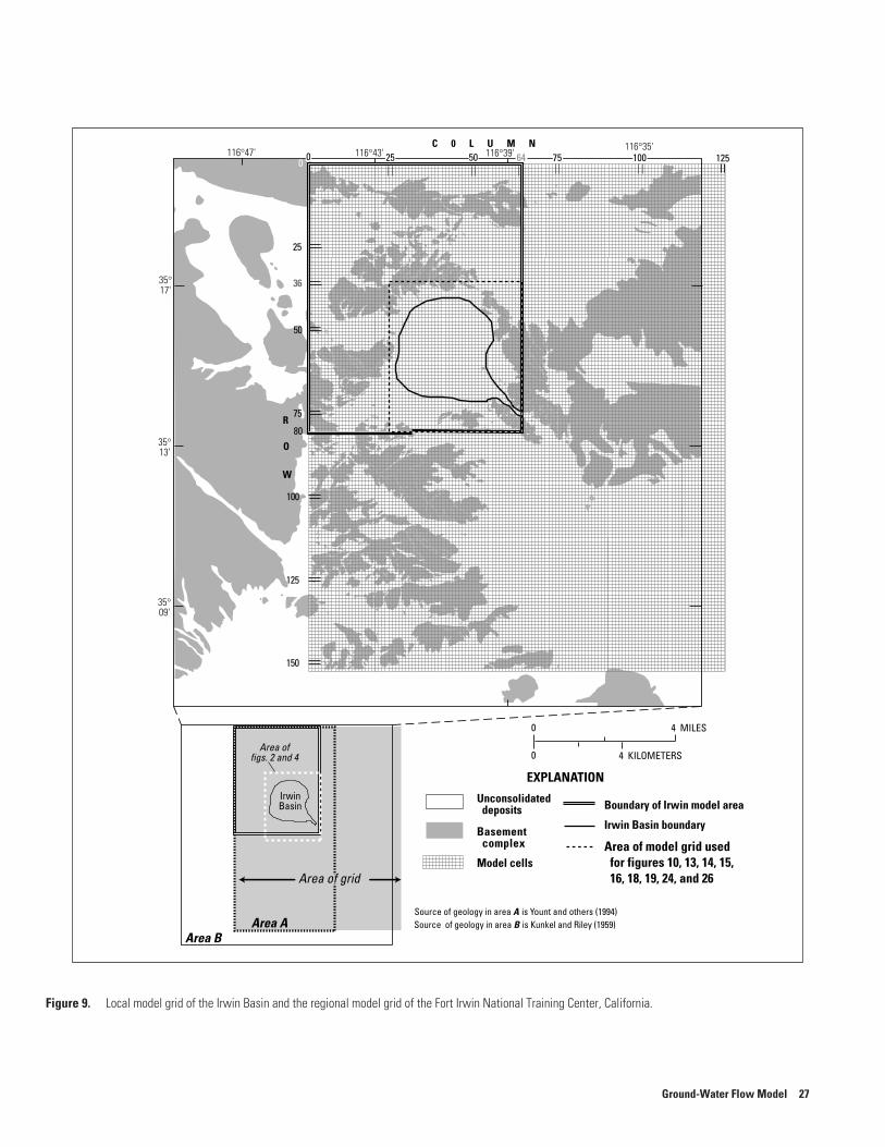
Figure 9. Local model grid of the Irwin Basin and the regional model grid of the Fort Irwin National Training Center, California.
Area AArea B
Area offigs. 2 and 4
35°09'
35°13'
35°17'
116°47' 116°43' 116°39'116°35'
IrwinBasin
0 75 10050
25
36
80
64 125C 0 L U M N
50
75
100
80
125
150
0 25
R
O
W
EXPLANATION
Basementcomplex
Unconsolidateddeposits
Model cells
Boundary of Irwin model area
Irwin Basin boundary
Area of model grid usedfor figures 10, 13, 14, 15,16, 18, 19, 24, and 26Area of grid
Source of geology in area A is Yount and others (1994)Source of geology in area B is Kunkel and Riley (1959)
0
0 4 KILOMETERS
4 MILES
Ground-Water Flow Model 27
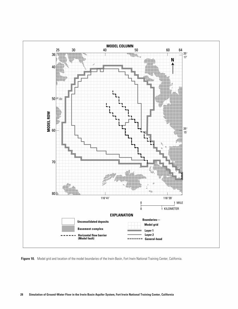
Figure 10. Model grid and location of the model boundaries of the Irwin Basin, Fort Irwin National Training Center, California.
25 30 40 50 6036
40
50
60
70
80
64MODEL COLUMN
MO
DEL
ROW
Basement complex
Unconsolidated deposits
Layer 1Layer 2
Boundaries—
Model grid
General-headHorizontal flow barrier(Model fault)
EXPLANATION
35°15'
116°39'116°41'
35°17'
1 KILOMETER
1 MILE
N
0
0
28 Simulation of Ground-Water Flow in the Irwin Basin Aquifer System, Fort Irwin National Training Center, California
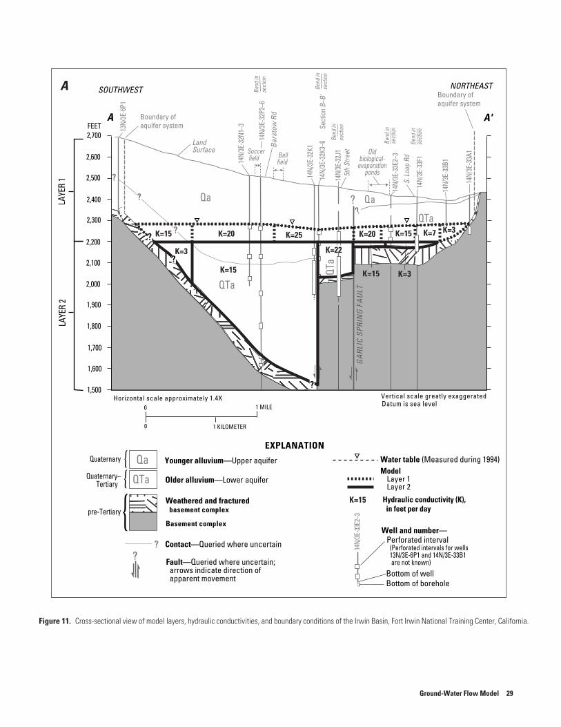
Figure 11. Cross-sectional view of model layers, hydraulic conductivities, and boundary conditions of the Irwin Basin, Fort Irwin National Training Center, California.
Boundary ofaquifer system
Boundary ofaquifer system
14N/
3E-3
2P2–
6
14N/
3E-3
2K1
14N/
3E-3
2K3–
6
14N/
3E-3
2J1
14N/
3E-3
3E2–
3
14N/
3E-3
3F1
14N/
3E-3
3A1
14N/
3E-3
2N1–
3
13N/
3E-6
P1
SOUTHWEST NORTHEAST
?Qa Qa
QTa
QTa
2,600
2,700FEET
2,500
2,400
2,300
2,200
2,100
2,000
1,900
1,800
1,700
1,600
1,500
A A'
Soccerfield
LandSurface
Ballfield
Sect
ion
B–B'
??
5th
Stre
et
S.Lo
opRd
Bar
stow
Rd
Oldbiological-
evaporationponds
GA
RLIC
SPRI
NG
FAU
LT
14N/
3E-3
3B1
Bend
inse
ctio
n
Bend
inse
ctio
n
Bend
inse
ctio
n
Bend
inse
ctio
n
Bend
inse
ctio
n
?
?
Hydraulic conductivity (K),in feet per day
ModelLayer 1Layer 2
K=15
K=3
K=20
K=15
K=25
K=22
K=15K=20
K=15 K=3
K=7 K=3
K=15
LAYE
R1
LAYE
R2
QTa
?
QTa
Water table (Measured during 1994)
? Contact—Queried where uncertain
Fault—Queried where uncertain;arrows indicate direction ofapparent movement
Well and number—Perforated interval
Bottom of boreholeBottom of well
EXPLANATION
14N/
3E-3
3E2–
3
}
Qa
Basement complex
Younger alluvium—Upper aquifer
Older alluvium—Lower aquifer
Weathered and fracturedbasement complex
Quaternary
Quaternary–Tertiary
{{
{pre-Tertiary
(Perforated intervals for wells13N/3E-6P1 and 14N/3E-33B1are not known)
Vertical scale greatly exaggeratedHorizontal scale approximately 1.4X
0
0 1 MILE Datum is sea level
1 KILOMETER
?
?
?
?
?
A
Ground-Water Flow Model 29
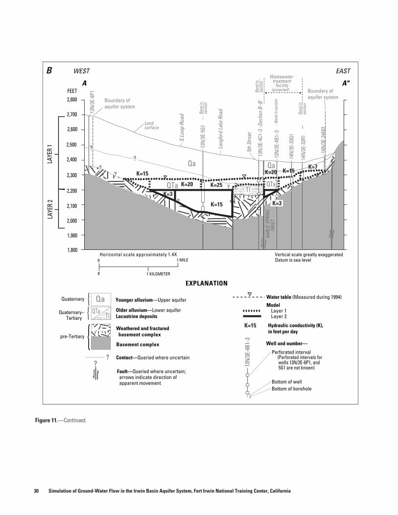
Figure 11.—Continued.
?
?
?
13N/
3E-4
C1–3
-Sec
tion
B–B'
13N/
3E-5
G1
14N/
3E-3
3Q1
14N/
3E-3
3R1
13N/
3E-4
B1–3
14N/
3E-3
4M2
13N/
3E-6
P1
?
Lang
ford
Lake
Road
5th
Stre
et
S.Lo
opRo
ad
GARL
ICSP
RING
FAUL
T
Qa Qa
QTa QTa
Wastewater-treatment
facility
Landsurface
(projected)
?
Bend
inse
ctio
n
Bend
inse
ctio
n
Bend
inse
ctio
n
Bend
inse
ctio
n
?
???
? K=15
K=20
K=3
K=3
K=25
K=7K=15
K=15
K=20
Hydraulic conductivity (K),in feet per day
ModelLayer 1Layer 2
K=15
Water table (Measured during 1994)
13N/
3E-4
B1–3 Well and number—
Perforated interval
Bottom of boreholeBottom of well
}
(Perforated intervals forwells 13N/3E-6P1, and5G1 are not known)
0
0 1 MILE Datum is sea level
1 KILOMETER
Vertical scale greatly exaggerated
?? Contact—Queried where uncertain
Fault—Queried where uncertain;arrows indicate direction ofapparent movement
EXPLANATION
Qa
Basement complex
Younger alluvium—Upper aquifer
Older alluvium—Lower aquiferLacustrine deposits
Weathered and fracturedbasement complex
Quaternary {{
{pre-Tertiary
QTaQuaternary–Tertiary
Horizontal scale approximately 1.4X
Tl
LAYE
R1
LAYE
R2
2,500
2,400
2,700
2,600
2,300
2,200
2,100
2,000
1,900
1,800
2,800FEET
WEST EAST
A A"Boundary ofaquifer system
Boundary ofaquifer system
B
Tl
30 Simulation of Ground-Water Flow in the Irwin Basin Aquifer System, Fort Irwin National Training Center, California
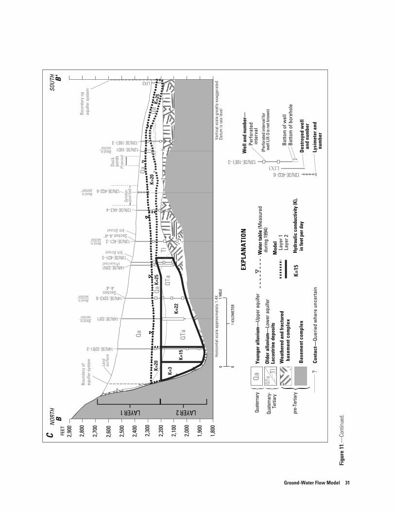
Figu
re 1
1.—
Cont
inue
d.
?
??
?
?
14N/3E-33N1
14N/3E-32B1–3
14N/3E-32K3–6
14N/3E-32F1
13N/3E-4D1–3
13N/3E-4C1–3
13N/3E-4Q2–6
13N/3E-4K2–4
13N/3E-10D113N/3E-10E1–3
Qa
QaQa
Qa
QTa
QTa
Sprin
kler-
pivot
field
Duck
pond
s
SectionA–A"
SectionA–A'
(Projected)
5thStreet
5thStreet
(Pro
jecte
d)
Bendinsection
Bendinsection
Bendinsection
Bendinsection
Bendinsection
LAYER1 LAYER2
?
?
?
SOUT
HN
ORTH
2,60
0
2,70
0
2,90
0
2,80
0
FEET
2,50
0
2,40
0
2,30
0
2,20
0
2,10
0
2,00
0
1,90
0
1,80
0
BB
'
?
K=20
K=25
K=20
K=22
K=15
K=25
?
K=3
?
LIX3
Hydr
aulic
cond
uctiv
ity(K
),in
feet
perd
ay
Mod
elLa
yer1
Laye
r2
K=15
Wat
erta
ble
(Mea
sure
ddu
ring
1994
)
Boun
dary
ofaq
uife
rsys
tem
Boun
dary
ogaq
uife
rsys
tem
?Co
ntac
t—Q
uerie
dw
here
unce
rtai
n
EXPL
AN
ATI
ON
LIX313N/3E-10E1–3
Lysi
met
eran
dnu
mbe
r
}
13N/3E-4Q2–6
Wel
land
num
ber—
Perf
orat
edin
terv
al
Bot
tom
ofbo
reho
leB
otto
mof
wel
l
Des
troy
edw
ell
and
num
ber
Qa
Bas
emen
tcom
plex
Youn
gera
lluvi
um—
Uppe
raqu
ifer
Old
eral
luvi
um—
Low
eraq
uife
rLa
cust
rine
depo
sits
Wea
ther
edan
dfr
actu
red
base
men
tcom
plex
Quat
erna
ry{ { {
pre-
Terti
ary
(Per
fora
ted
inte
rval
for
wel
lLIX
-3is
notk
now
n)QT
aQu
ater
nary
-Te
rtiar
yTl
01
KILO
MET
ER
Vert
ical
scal
egr
eatly
exag
gera
ted
Datu
mis
sea
leve
lHo
rizon
tals
cale
appr
oxim
atel
y1.
4X0
1M
ILE
? ?
Land
surfa
ce
C
Tl
Ground-Water Flow Model 31
Model Boundaries
The model boundaries (figs. 10 and 11) were determined from the interpretations of the geology of the Irwin Basin. The lateral boundaries of the model coincide with the lateral boundaries of the aquifer system. The top boundary of the model, the water table, is simulated as a free-surface boundary (unconfined) to allow it to move vertically in response to changes between inflow and outflow. No-flow boundaries are used around and below the modeled area to represent contact with the basement complex and ground-water divides (figs. 10 and 11). The no-flow boundary indicates that there is no exchange of water between the model cell and the area outside the model.
The HFB package simulates faults that impede the horizontal flow of ground water; the boundary was simulated using the HFB package by Hsieh and Freckleton (1993). Flow across this boundary is proportional to the hydraulic-head difference between adjacent cells. The function of each barrier is to lower the horizontal conductances between the two adjacent model cells. In this model, the flow barrier is defined by a hydraulic characteristic. For confined aquifers, the hydraulic characteristic is the barrier transmissivity divided by the width of the barrier and has units of LT-1. For unconfined aquifers, the hydraulic characteristic is the barrier hydraulic conductivity divided by the width of the barrier and has units of T-1. This characteristic is determined during the calibration process.
The Garlic Spring Fault and a parallel unnamed fault were simulated using the horizontal-flow-barrier package (fig. 10). Water-quality data from Densmore and Londquist (1997) indicate that these faults act as a partial barrier to ground-water flow, suggesting that horizontal flow across the Garlic Spring Fault, primarily in the lower aquifer, is impeded. Based on model calibration, the hydraulic characteristics for the Garlic Spring Fault were assigned values of 0.002 ft/day and 0.002 ft/day for layer 1 and 2, respectively. The hydraulic characteristics for the parallel unnamed fault were assigned values of 0.01 ft/day and 0.01 ft/day for layer 1 and 2, respectively, thereby allowing
slightly more horizontal flow across the unnamed fault than across the Garlic Spring Fault. Because it is not known if these faults cross the entire basin, the faults were modeled as only partly crossing the basin. Changes in the fault conductance made during calibration had minimal effect on the simulated water-level changes.
The GHB package (McDonald and Harbaugh, 1988, p. 11-1; table 3) was used to simulate underflow from layer 1 through the unnamed wash near Garlic Spring. A general-head boundary simulates a source of water outside the model area that either supplies water to, or receives water from, adjacent cells in proportion to the hydraulic-head differences between the source and model cell.
The exchange rate of water between the model cell and the outside source or sink is given by the equation
where
Values of C were initially calculated using the equation
where
Q is the rate of flow into or out of the model cell [L3/T],
C is the conductance between the external source or sink and the model cell [L2/T],
HB is the head assigned to the external source or sink [L], and
h is the hydraulic head within the model cell [L].
K is the hydraulic conductivity between the model cell and the boundary head [L/T],
A is the cross-sectional area perpendicular to flow [L2], and
L is the flow distance [L].
Q C HB h–( )=
C KA L⁄ ,=
32 Simulation of Ground-Water Flow in the Irwin Basin Aquifer System, Fort Irwin National Training Center, California
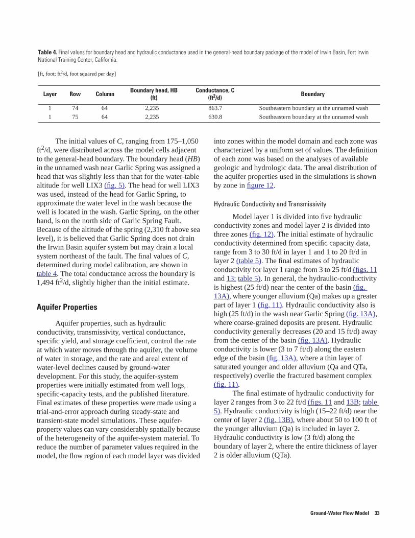
The initial values of C, ranging from 175–1,050 ft2/d, were distributed across the model cells adjacent to the general-head boundary. The boundary head (HB) in the unnamed wash near Garlic Spring was assigned a head that was slightly less than that for the water-table altitude for well LIX3 (fig. 5). The head for well LIX3 was used, instead of the head for Garlic Spring, to approximate the water level in the wash because the well is located in the wash. Garlic Spring, on the other hand, is on the north side of Garlic Spring Fault. Because of the altitude of the spring (2,310 ft above sea level), it is believed that Garlic Spring does not drain the Irwin Basin aquifer system but may drain a local system northeast of the fault. The final values of C, determined during model calibration, are shown in table 4. The total conductance across the boundary is 1,494 ft2/d, slightly higher than the initial estimate.
Aquifer Properties
Aquifer properties, such as hydraulic conductivity, transmissivity, vertical conductance, specific yield, and storage coefficient, control the rate at which water moves through the aquifer, the volume of water in storage, and the rate and areal extent of water-level declines caused by ground-water development. For this study, the aquifer-system properties were initially estimated from well logs, specific-capacity tests, and the published literature. Final estimates of these properties were made using a trial-and-error approach during steady-state and transient-state model simulations. These aquifer-property values can vary considerably spatially because of the heterogeneity of the aquifer-system material. To reduce the number of parameter values required in the model, the flow region of each model layer was divided
into zones within the model domain and each zone was characterized by a uniform set of values. The definition of each zone was based on the analyses of available geologic and hydrologic data. The areal distribution of the aquifer properties used in the simulations is shown by zone in figure 12.
Hydraulic Conductivity and Transmissivity
Model layer 1 is divided into five hydraulic conductivity zones and model layer 2 is divided into three zones (fig. 12). The initial estimate of hydraulic conductivity determined from specific capacity data, range from 3 to 30 ft/d in layer 1 and 1 to 20 ft/d in layer 2 (table 5). The final estimates of hydraulic conductivity for layer 1 range from 3 to 25 ft/d (figs. 11 and 13; table 5). In general, the hydraulic-conductivity is highest (25 ft/d) near the center of the basin (fig. 13A), where younger alluvium (Qa) makes up a greater part of layer 1 (fig. 11). Hydraulic conductivity also is high (25 ft/d) in the wash near Garlic Spring (fig. 13A), where coarse-grained deposits are present. Hydraulic conductivity generally decreases (20 and 15 ft/d) away from the center of the basin (fig. 13A). Hydraulic conductivity is lower (3 to 7 ft/d) along the eastern edge of the basin (fig. 13A), where a thin layer of saturated younger and older alluvium (Qa and QTa, respectively) overlie the fractured basement complex (fig. 11).
The final estimate of hydraulic conductivity for layer 2 ranges from 3 to 22 ft/d (figs. 11 and 13B; table 5). Hydraulic conductivity is high (15–22 ft/d) near the center of layer 2 (fig. 13B), where about 50 to 100 ft of the younger alluvium (Qa) is included in layer 2. Hydraulic conductivity is low (3 ft/d) along the boundary of layer 2, where the entire thickness of layer 2 is older alluvium (QTa).
Table 4. Final values for boundary head and hydraulic conductance used in the general-head boundary package of the model of Irwin Basin, Fort Irwin National Training Center, California.
[ft, foot; ft2/d, foot squared per day]
Layer Row ColumnBoundary head, HB
(ft)Conductance, C
(ft2/d)Boundary
1 74 64 2,235 863.7 Southeastern boundary at the unnamed wash
1 75 64 2,235 630.8 Southeastern boundary at the unnamed wash
Ground-Water Flow Model 33
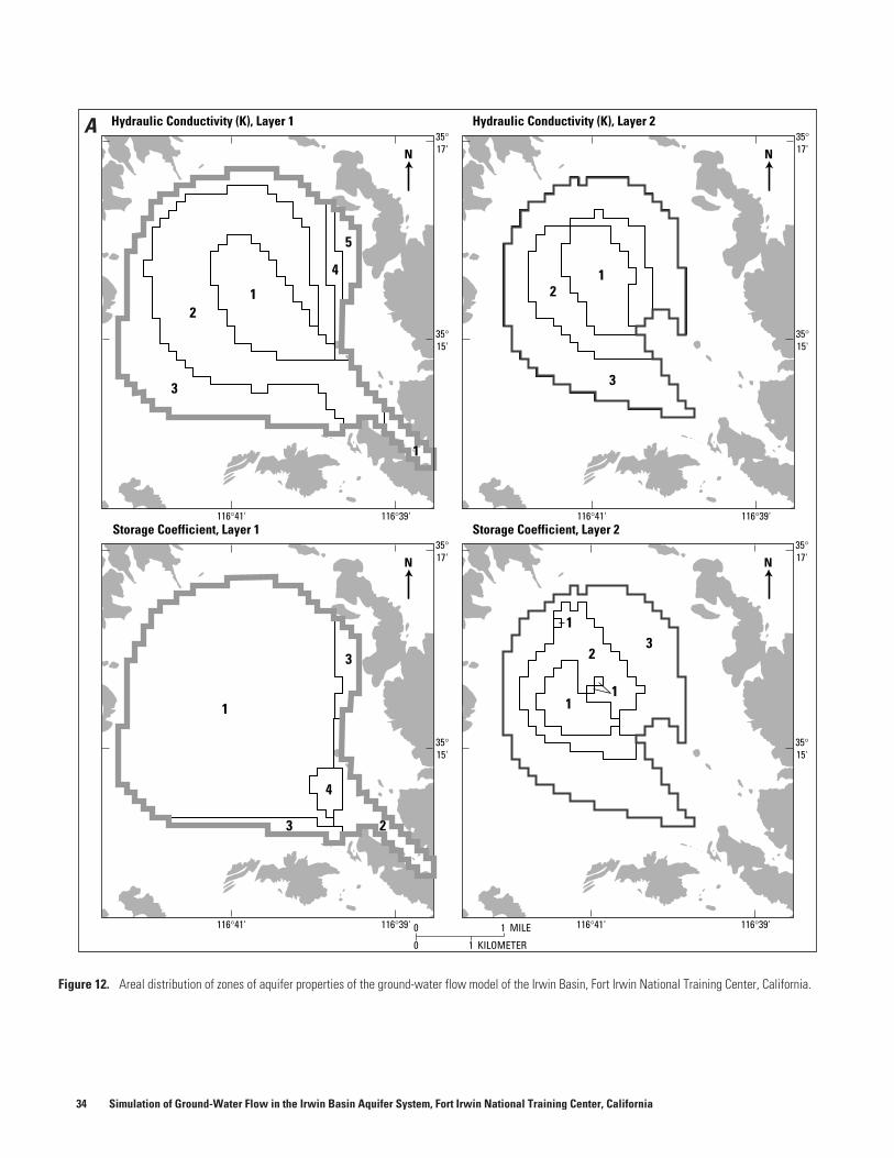
Figure 12. Areal distribution of zones of aquifer properties of the ground-water flow model of the Irwin Basin, Fort Irwin National Training Center, California.
12
3
1
1
2
3
4
5
35°15'
116°39'116°41'
35°17'N
35°15'
116°39'116°41'
35°17'N
35°15'
116°39'116°41'
35°17'N
0 1 KILOMETER
0 1 MILE
A Hydraulic Conductivity (K), Layer 1 Hydraulic Conductivity (K), Layer 2
Storage Coefficient, Layer 2
1 1
1
1
4
3
33
2
2
35°15'
116°39'116°41'
35°17'N
Storage Coefficient, Layer 1
34 Simulation of Ground-Water Flow in the Irwin Basin Aquifer System, Fort Irwin National Training Center, California
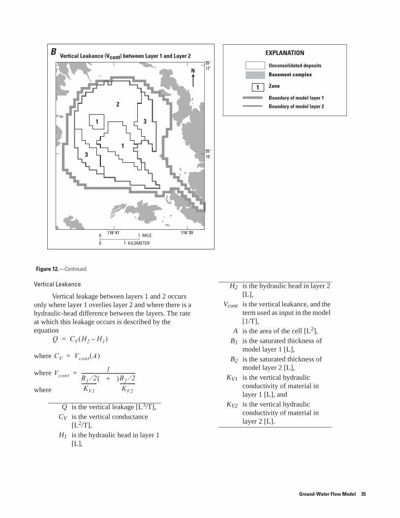
Vertical Leakance
Vertical leakage between layers 1 and 2 occurs only where layer 1 overlies layer 2 and where there is a hydraulic-head difference between the layers. The rate at which this leakage occurs is described by the equation
where
where
where
Q is the vertical leakage [L3/T],CV is the vertical conductance
[L2/T],H1 is the hydraulic head in layer 1
[L],
Q CV H2 H1–( )=
CV Vcont A( )=
Vcont1
B1 2⁄KV1
-------------+( )B2 2⁄
KV2-------------
---------------------------------------------=
H2 is the hydraulic head in layer 2 [L],
Vcont is the vertical leakance, and the term used as input in the model [1/T],
A is the area of the cell [L2],B1 is the saturated thickness of
model layer 1 [L],B2 is the saturated thickness of
model layer 2 [L],KV1 is the vertical hydraulic
conductivity of material in layer 1 [L], and
KV2 is the vertical hydraulic conductivity of material in layer 2 [L].
Figure 12.—Continued.
1
1
2
3
3
35°15'
116°39'116°41'
35°17'N
0 1 KILOMETER
0 1 MILE
Vertical Leakance (Vcont) between Layer 1 and Layer 2B
1
Basement complex
Zone
Unconsolidated deposits
EXPLANATION
Boundary of model layer 1
Boundary of model layer 2
Ground-Water Flow Model 35
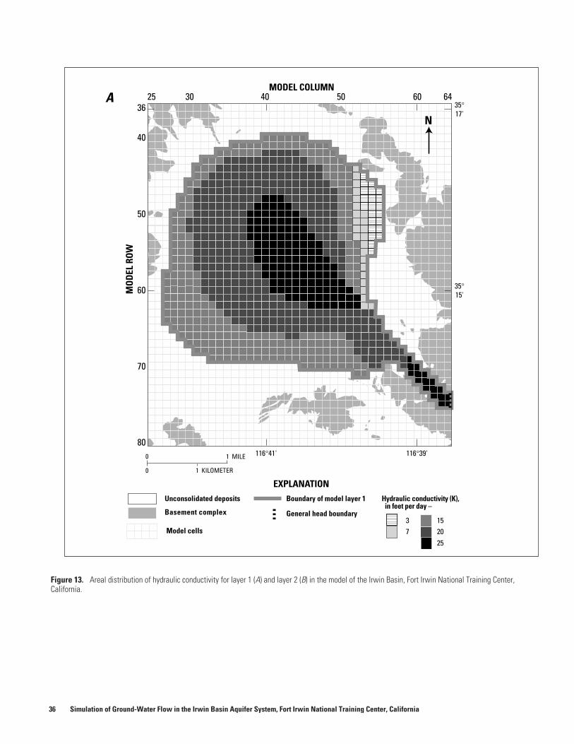
Figure 13. Areal distribution of hydraulic conductivity for layer 1 (A) and layer 2 (B) in the model of the Irwin Basin, Fort Irwin National Training Center, California.
25 30 40 50 6036
40
50
60
70
80
64MODEL COLUMN
MO
DEL
ROW
35°15'
116°39'116°41'
35°17'
N
Basement complex
Unconsolidated deposits
Model cells 73
2015
25
Hydraulic conductivity (K),in feet per day –
Boundary of model layer 1
General head boundary
EXPLANATION
1 KILOMETER
1 MILE
A
0
0
36 Simulation of Ground-Water Flow in the Irwin Basin Aquifer System, Fort Irwin National Training Center, California
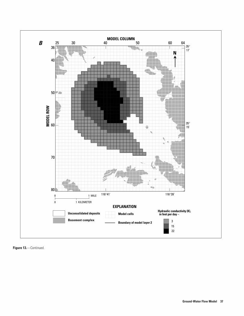
Figure 13.—Continued.
25 30 40 50 6036
40
50
60
70
80
64MODEL COLUMN
MO
DEL
ROW
35°15'
116°39'116°41'
35°17'
N
Basement complexBoundary of model layer 2
Unconsolidated deposits Model cells
3
2215
EXPLANATIONHydraulic conductivity (K),in feet per day –
1 KILOMETER
1 MILE
B
0
0
Ground-Water Flow Model 37
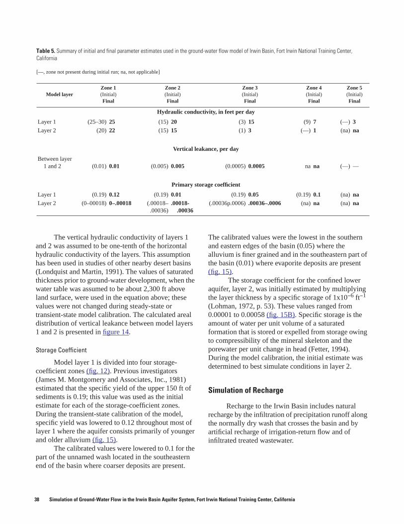
The vertical hydraulic conductivity of layers 1 and 2 was assumed to be one-tenth of the horizontal hydraulic conductivity of the layers. This assumption has been used in studies of other nearby desert basins (Londquist and Martin, 1991). The values of saturated thickness prior to ground-water development, when the water table was assumed to be about 2,300 ft above land surface, were used in the equation above; these values were not changed during steady-state or transient-state model calibration. The calculated areal distribution of vertical leakance between model layers 1 and 2 is presented in figure 14.
Storage Coefficient
Model layer 1 is divided into four storage-coefficient zones (fig. 12). Previous investigators (James M. Montgomery and Associates, Inc., 1981) estimated that the specific yield of the upper 150 ft of sediments is 0.19; this value was used as the initial estimate for each of the storage-coefficient zones. During the transient-state calibration of the model, specific yield was lowered to 0.12 throughout most of layer 1 where the aquifer consists primarily of younger and older alluvium (fig. 15).
The calibrated values were lowered to 0.1 for the part of the unnamed wash located in the southeastern end of the basin where coarser deposits are present.
The calibrated values were the lowest in the southern and eastern edges of the basin (0.05) where the alluvium is finer grained and in the southeastern part of the basin (0.01) where evaporite deposits are present (fig. 15).
The storage coefficient for the confined lower aquifer, layer 2, was initially estimated by multiplying the layer thickness by a specific storage of 1x10⁻⁶ ft−1 (Lohman, 1972, p. 53). These values ranged from 0.00001 to 0.00058 (fig. 15B). Specific storage is the amount of water per unit volume of a saturated formation that is stored or expelled from storage owing to compressibility of the mineral skeleton and the porewater per unit change in head (Fetter, 1994). During the model calibration, the initial estimate was determined to best simulate conditions in layer 2.
Simulation of Recharge
Recharge to the Irwin Basin includes natural recharge by the infiltration of precipitation runoff along the normally dry wash that crosses the basin and by artificial recharge of irrigation-return flow and of infiltrated treated wastewater.
Table 5. Summary of initial and final parameter estimates used in the ground-water flow model of Irwin Basin, Fort Irwin National Training Center, California
[—, zone not present during initial run; na, not applicable]
Model layerZone 1(Initial) Final
Zone 2(Initial) Final
Zone 3(Initial)Final
Zone 4(Initial) Final
Zone 5(Initial) Final
Hydraulic conductivity, in feet per day
Layer 1 (25–30) 25 (15) 20 (3) 15 (9) 7 (—) 3
Layer 2 (20) 22 (15) 15 (1) 3 (—) 1 (na) na
Vertical leakance, per day
Between layer 1 and 2 (0.01) 0.01 (0.005) 0.005 (0.0005) 0.0005 na na (—) —
Primary storage coefficient
Layer 1 (0.19) 0.12 (0.19) 0.01 (0.19) 0.05 (0.19) 0.1 (na) na
Layer 2 (0–00018) 0–.00018 (.00018–.00036)
.00018-.00036
(.00036p.0006) .00036–.0006 (na) na (na) na
38 Simulation of Ground-Water Flow in the Irwin Basin Aquifer System, Fort Irwin National Training Center, California
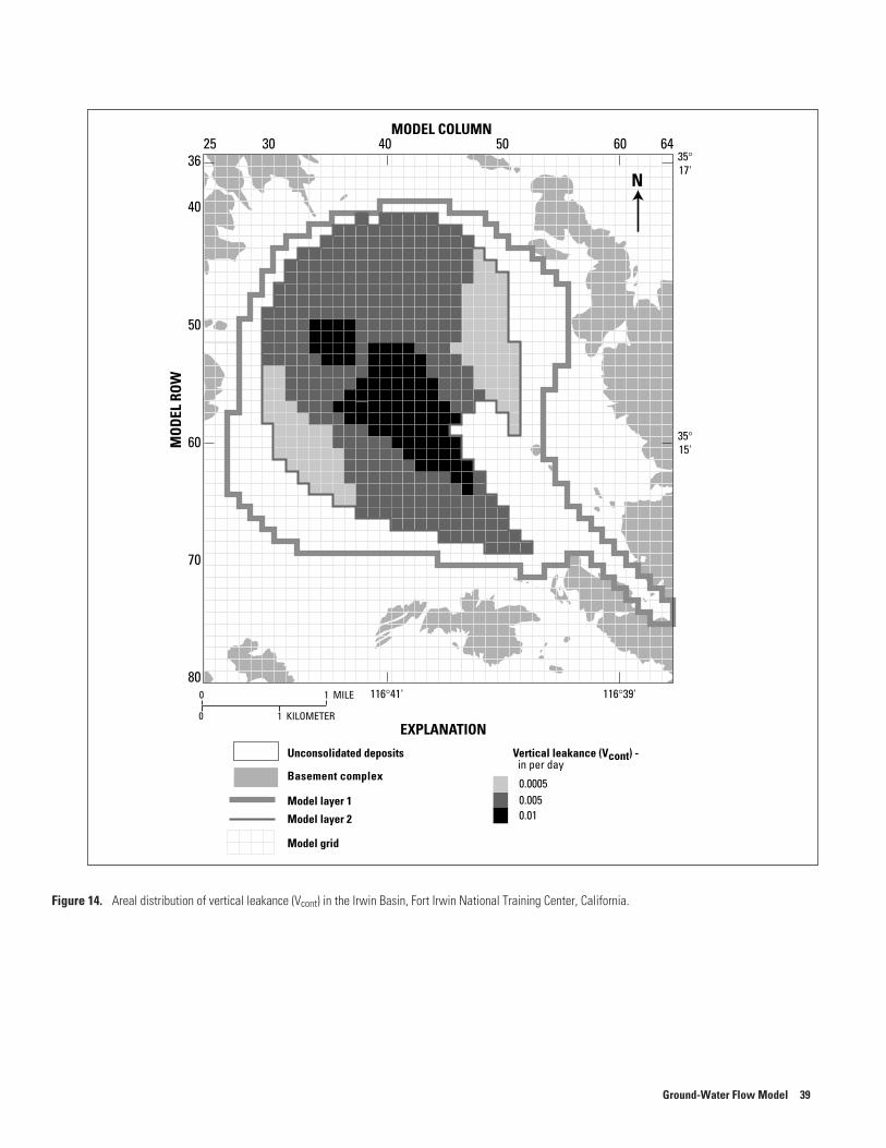
Figure 14. Areal distribution of vertical leakance (Vcont) in the Irwin Basin, Fort Irwin National Training Center, California.
25 30 40 50 6036
40
50
60
70
80
64MODEL COLUMN
MO
DEL
ROW
35°15'
116°39'116°41'
35°17'
N
0
0 1 KILOMETER
1 MILE
Basement complex
Unconsolidated deposits
Model grid
Model layer 1
Model layer 2
0.00050.0050.01
Vertical leakance (Vcont) -in per day
EXPLANATION
Ground-Water Flow Model 39
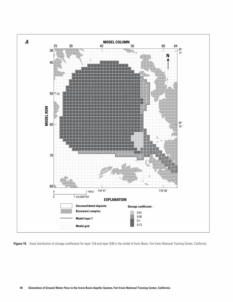
Figure 15. Areal distribution of storage coefficients for layer 1(A) and layer 2(B) in the model of Irwin Basin, Fort Irwin National Training Center, California.
25 30 40 50 6036
40
50
60
70
80
64MODEL COLUMN
MO
DEL
ROW
35°15'
116°39'116°41'
35°17'
N
0
0 1 KILOMETER
1 MILE
Basement complex
Unconsolidated deposits
Model grid
Model layer 1
0.010.050.10.12
Storage coefficient -
EXPLANATION
A
40 Simulation of Ground-Water Flow in the Irwin Basin Aquifer System, Fort Irwin National Training Center, California
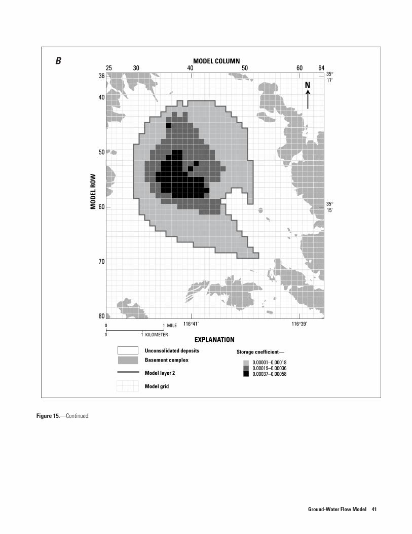
Figure 15.—Continued.
25 30 40 50 6036
40
50
60
70
80
64MODEL COLUMN
MO
DEL
ROW
35°15'
116°39'116°41'
35°17'
N
0
0 1 KILOMETER
1 MILE
Basement complex
Unconsolidated deposits
Model grid
Model layer 2
Storage coefficient—
EXPLANATION
B
0.00001–0.000180.00019–0.000360.00037–0.00058
Ground-Water Flow Model 41
Natural Recharge
As previously stated, natural recharge in the Irwin Basin is solely by infiltration of precipitation runoff within the Irwin drainage basin (fig. 1). It was assumed that areal recharge from direct infiltration of precipitation was insignificant because of the infrequent occurrence of these events and because of the low precipitation and high evaporation rates in the study area. Recent work in the upper Mojave Basin by Izbicki and others (2000) shows that infiltration does not occur at depths below the root zone except in areas of some intermittent washes in arid desert environments. Thus, natural recharge was simulated only along the intermittent wash (fig. 16) that was formed by runoff from Northwest and Southwest Ridges (fig. 2) using the areal recharge package (RECH) developed by McDonald and Harbaugh (1988, p. 7–1).
The initial estimate of natural recharge from precipitation runoff used to calibrate the model was 150 acre-ft/yr (C.F. Hostrup and Associates, 1955). This estimate was lowered to about 50 acre-ft/yr during calibration of the steady-state and transient-state simulations. Two-thirds of the total recharge was simulated to infiltrate into the upper one-third of the wash; the remaining one-third of total recharge was simulated to infiltrate into the lower two-thirds of the wash (fig. 16).
Artificial Recharge
Artificial recharge to the basin was divided into two categories: infiltration of treated wastewater that was diverted to the base golf course, driving range, sprinkler-pivot field, and duck ponds; and irrigation-return flow from lawns and fields in the base housing areas that were irrigated using ground water. Artificial recharge was simulated using the areal recharge package (RECH) developed by McDonald and Harbaugh (1988) which distributed additional recharge to the cells underlying the wastewater disposal area and the irrigated areas. The areal distribution of artificial recharge is presented in figure 16.
Estimates of ground-water recharge from wastewater infiltration presented by Densmore and Londquist (1997) and updated for this study (table 3) were used as the initial estimates for the artificial
recharge. These values were modified during calibration of the transient-state model (table 6). The final calibrated values of wastewater recharge generally were higher than the initial estimates for 1955–85 and lower than the initial estimates for 1991–94. The lower calibrated values of wastewater recharge for 1991–94 may reflect a decrease in water disposed at the wastewater-treatment facility owing to better conservation practices at base housing. The lower values also may reflect that more of the pumped water was being used outside of Irwin Basin. It is also possible that during this time, more of the wastewater was being distributed to the sprinkler-pivot field where more evaporation could occur which would result in less artificial recharge. The final estimates of irrigation-return flow generally were the same or lower than the initial estimates prior to 1964 and higher than the initial estimates for 1965–99.
Simulation of Discharge
Ground-water pumpage is the main discharge from the basin. Ground-water pumpage in the Irwin Basin began in 1941 when the first two wells were drilled to supply water at Camp Irwin. All the water used at the base during 1941–66 was supplied from wells in the Irwin Basin (fig. 17). Pumping from the Bicycle Basin in 1967 and the Langford Basin in 1992 allowed for a reduction in pumping from the Irwin Basin. Although annual pumpage (fig. 17) was estimated during previous studies, the distribution of pumpage among the individual wells for 1941–89 was not reported for the Irwin Basin. Therefore, the distribution of pumpage for this period was estimated as a percentage of water based on well-capacity data from pump tests. For this study, annual pumpage for 1990–99 was obtained from records provided by Fort Irwin personnel (Rene Quinones, Walt Young, and Suzanne Beauchamp, Fort Irwin National Training Center, written commun., 1996, 1998, 2000). The pumpage from each model layer was distributed such that about two-thirds of the total pumpage per well comes from layer 1 and about one-third comes from layer 2. This estimated distribution was based on results of wellbore-flow tests described by Densmore and Londquist (1997).
42 Simulation of Ground-Water Flow in the Irwin Basin Aquifer System, Fort Irwin National Training Center, California
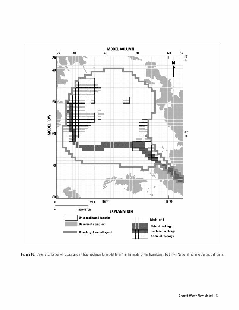
Figure 16. Areal distribution of natural and artificial recharge for model layer 1 in the model of the Irwin Basin, Fort Irwin National Training Center, California.
25 30 40 50 6036
40
50
60
70
80
64MODEL COLUMN
MO
DEL
ROW
35°15'
116°39'116°41'
35°17'
N
Boundary of model layer 1
0
0 1 KILOMETER
1 MILE
Basement complex
Unconsolidated depositsModel grid
Natural recharge
Combined recharge
Artificial recharge
EXPLANATION
Ground-Water Flow Model 43
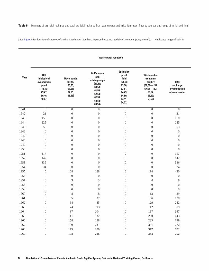
Table 6. Summary of artificial recharge and total artificial recharge from wastewater and irrigation-return flow by sources and range of initial and final
[See figure 5 for location of sources of artificial recharge. Numbers in parentheses are model cell numbers (row;column). —> indicates range of cells in
Year
Wastewater recharge
Old biological
evaporation pond
(49,46;49,47;50,46;50;47)
Duck ponds(64,55;65,55;66,55;67,55;68,55)
Golf courseand
driving range(59,53;60,53;61,53;62,53;62,54;63,53;63,54)
Sprinkler-pivotfield
(63,49;63,50;63,51;64,49;64,50;64,51;64,52)
Wastewater-treatment
facility(56,52—>53;57,52—>53;
58,52;59,52;56,52)
Totalrecharge
by infiltrationof wastewater
1941 0 0 0 0 0 0
1942 21 0 0 0 0 21
1943 150 0 0 0 0 150
1944 225 0 0 0 0 225
1945 53 0 0 0 0 53
1946 0 0 0 0 0 0
1947 0 0 0 0 0 0
1948 0 0 0 0 0 0
1949 0 0 0 0 0 0
1950 0 0 0 0 0 0
1951 117 0 0 0 0 117
1952 142 0 0 0 0 142
1953 336 0 0 0 0 336
1954 334 0 0 0 0 334
1955 0 108 128 0 194 430
1956 0 0 0 0 0 0
1957 0 3 3 0 4 9
1958 0 0 0 0 0 0
1959 0 0 0 0 0 0
1960 0 8 8 0 13 29
1961 0 35 37 0 56 128
1962 0 68 85 0 129 282
1963 0 74 93 0 142 309
1964 0 87 104 0 157 347
1965 0 111 132 0 200 443
1966 0 158 188 0 283 629
1967 0 190 231 0 351 772
1968 0 175 209 0 317 702
1969 0 198 236 0 358 792
44 Simulation of Ground-Water Flow in the Irwin Basin Aquifer System, Fort Irwin National Training Center, California
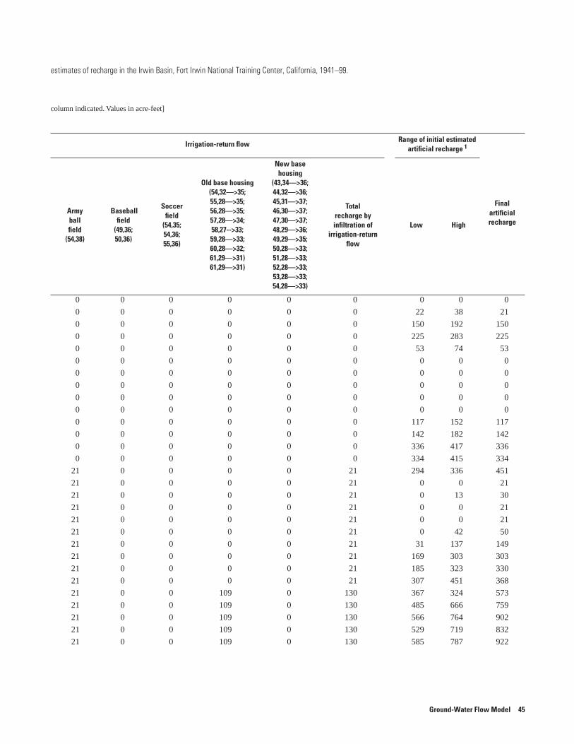
Ground-Water Flow Model 45
estimates of recharge in the Irwin Basin, Fort Irwin National Training Center, California, 1941–99.
column indicated. Values in acre-feet]
Irrigation-return flowRange of initial estimated
artificial recharge 1
Final artificial recharge
Armyballfield
(54,38)
Baseballfield
(49,36;50,36)
Soccerfield
(54,35;54,36;55,36)
Old base housing(54,32—>35;55,28—>35;56,28—>35;57,28—>34;58,27-->33;59,28—>33;60,28—>32;61,29—>31)61,29—>31)
New basehousing
(43,34—>36; 44,32—>36;45,31—>37; 46,30—>37;47,30—>37; 48,29—>36;49,29—>35; 50,28—>33;51,28—>33; 52,28—>33;53,28—>33; 54,28—>33)
Totalrecharge by infiltration of
irrigation-return flow
Low High
0 0 0 0 0 0 0 0 0
0 0 0 0 0 0 22 38 21
0 0 0 0 0 0 150 192 150
0 0 0 0 0 0 225 283 225
0 0 0 0 0 0 53 74 53
0 0 0 0 0 0 0 0 0
0 0 0 0 0 0 0 0 0
0 0 0 0 0 0 0 0 0
0 0 0 0 0 0 0 0 0
0 0 0 0 0 0 0 0 0
0 0 0 0 0 0 117 152 117
0 0 0 0 0 0 142 182 142
0 0 0 0 0 0 336 417 336
0 0 0 0 0 0 334 415 334
21 0 0 0 0 21 294 336 451
21 0 0 0 0 21 0 0 21
21 0 0 0 0 21 0 13 30
21 0 0 0 0 21 0 0 21
21 0 0 0 0 21 0 0 21
21 0 0 0 0 21 0 42 50
21 0 0 0 0 21 31 137 149
21 0 0 0 0 21 169 303 303
21 0 0 0 0 21 185 323 330
21 0 0 0 0 21 307 451 368
21 0 0 109 0 130 367 324 573
21 0 0 109 0 130 485 666 759
21 0 0 109 0 130 566 764 902
21 0 0 109 0 130 529 719 832
21 0 0 109 0 130 585 787 922
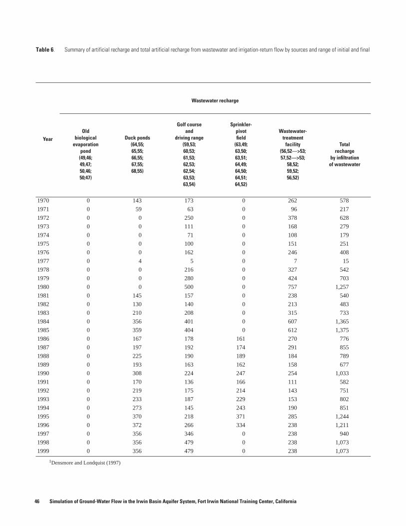
Table 6. Summary of artificial recharge and total artificial recharge from wastewater and irrigation-return flow by sources and range of initial and final
1Densmore and Londquist (1997)
Year
Wastewater recharge
Old biological
evaporation pond
(49,46;49,47;50,46;50;47)
Duck ponds(64,55;65,55;66,55;67,55;68,55)
Golf courseand
driving range(59,53;60,53;61,53;62,53;62,54;63,53;63,54)
Sprinkler-pivotfield
(63,49;63,50;63,51;64,49;64,50;64,51;64,52)
Wastewater-treatment
facility(56,52—>53;57,52—>53;
58,52;59,52;56,52)
Total recharge
by infiltrationof wastewater
1970 0 143 173 0 262 578
1971 0 59 63 0 96 217
1972 0 0 250 0 378 628
1973 0 0 111 0 168 279
1974 0 0 71 0 108 179
1975 0 0 100 0 151 251
1976 0 0 162 0 246 408
1977 0 4 5 0 7 15
1978 0 0 216 0 327 542
1979 0 0 280 0 424 703
1980 0 0 500 0 757 1,257
1981 0 145 157 0 238 540
1982 0 130 140 0 213 483
1983 0 210 208 0 315 733
1984 0 356 401 0 607 1,365
1985 0 359 404 0 612 1,375
1986 0 167 178 161 270 776
1987 0 197 192 174 291 855
1988 0 225 190 189 184 789
1989 0 193 163 162 158 677
1990 0 308 224 247 254 1,033
1991 0 170 136 166 111 582
1992 0 219 175 214 143 751
1993 0 233 187 229 153 802
1994 0 273 145 243 190 851
1995 0 370 218 371 285 1,244
1996 0 372 266 334 238 1,211
1997 0 356 346 0 238 940
1998 0 356 479 0 238 1,073
1999 0 356 479 0 238 1,073
46 Simulation of Ground-Water Flow in the Irwin Basin Aquifer System, Fort Irwin National Training Center, California
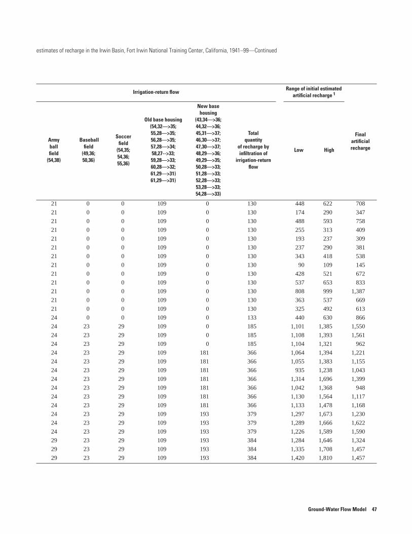
estimates of recharge in the Irwin Basin, Fort Irwin National Training Center, California, 1941–99—Continued
Irrigation-return flowRange of initial estimated
artificial recharge 1
Final artificial recharge
Armyballfield
(54,38)
Baseballfield
(49,36;50,36)
Soccerfield
(54,35;54,36;55,36)
Old base housing(54,32—>35;55,28—>35;56,28—>35;57,28—>34;58,27-->33;59,28—>33;60,28—>32;61,29—>31)61,29—>31)
New basehousing
(43,34—>36; 44,32—>36;45,31—>37; 46,30—>37;47,30—>37; 48,29—>36;49,29—>35; 50,28—>33;51,28—>33; 52,28—>33;53,28—>33; 54,28—>33)
Totalquantity
of recharge by infiltration of
irrigation-return flow
Low High
21 0 0 109 0 130 448 622 708
21 0 0 109 0 130 174 290 347
21 0 0 109 0 130 488 593 758
21 0 0 109 0 130 255 313 409
21 0 0 109 0 130 193 237 309
21 0 0 109 0 130 237 290 381
21 0 0 109 0 130 343 418 538
21 0 0 109 0 130 90 109 145
21 0 0 109 0 130 428 521 672
21 0 0 109 0 130 537 653 833
21 0 0 109 0 130 808 999 1,387
21 0 0 109 0 130 363 537 669
21 0 0 109 0 130 325 492 613
24 0 0 109 0 133 440 630 866
24 23 29 109 0 185 1,101 1,385 1,550
24 23 29 109 0 185 1,108 1,393 1,561
24 23 29 109 0 185 1,104 1,321 962
24 23 29 109 181 366 1,064 1,394 1,221
24 23 29 109 181 366 1,055 1,383 1,155
24 23 29 109 181 366 935 1,238 1,043
24 23 29 109 181 366 1,314 1,696 1,399
24 23 29 109 181 366 1,042 1,368 948
24 23 29 109 181 366 1,130 1,564 1,117
24 23 29 109 181 366 1,133 1,478 1,168
24 23 29 109 193 379 1,297 1,673 1,230
24 23 29 109 193 379 1,289 1,666 1,622
24 23 29 109 193 379 1,226 1,589 1,590
29 23 29 109 193 384 1,284 1,646 1,324
29 23 29 109 193 384 1,335 1,708 1,457
29 23 29 109 193 384 1,420 1,810 1,457
Ground-Water Flow Model 47
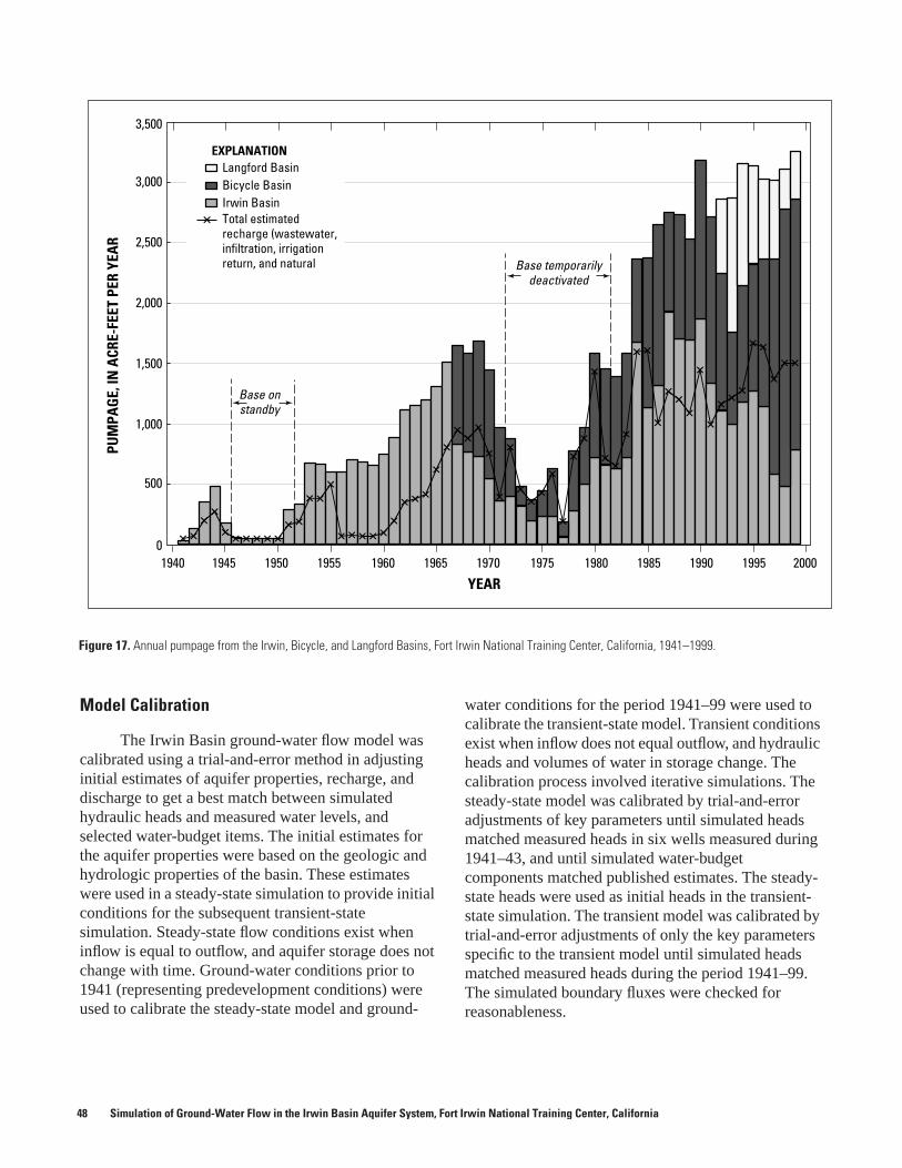
Figure 17. Annual pumpage from the Irwin, Bicycle, and Langford Basins, Fort Irwin National Training Center, California, 1941–1999.
0
500
1,000
1,500
2,000
2,500
3,000
3,500
1940 1945 1950 1955 1960 1965 1970 1975 1980 1985 1990 1995 2000
YEAR
PUM
PAG
E,IN
ACR
E-FE
ETPE
RYE
AR
Langford BasinBicycle BasinIrwin BasinTotal estimatedrecharge (wastewater,infiltration, irrigationreturn, and natural
EXPLANATION
Base onstandby
Base temporarilydeactivated
Model Calibration
The Irwin Basin ground-water flow model was calibrated using a trial-and-error method in adjusting initial estimates of aquifer properties, recharge, and discharge to get a best match between simulated hydraulic heads and measured water levels, and selected water-budget items. The initial estimates for the aquifer properties were based on the geologic and hydrologic properties of the basin. These estimates were used in a steady-state simulation to provide initial conditions for the subsequent transient-state simulation. Steady-state flow conditions exist when inflow is equal to outflow, and aquifer storage does not change with time. Ground-water conditions prior to 1941 (representing predevelopment conditions) were used to calibrate the steady-state model and ground-
water conditions for the period 1941–99 were used to calibrate the transient-state model. Transient conditions exist when inflow does not equal outflow, and hydraulic heads and volumes of water in storage change. The calibration process involved iterative simulations. The steady-state model was calibrated by trial-and-error adjustments of key parameters until simulated heads matched measured heads in six wells measured during 1941–43, and until simulated water-budget components matched published estimates. The steady-state heads were used as initial heads in the transient-state simulation. The transient model was calibrated by trial-and-error adjustments of only the key parameters specific to the transient model until simulated heads matched measured heads during the period 1941–99. The simulated boundary fluxes were checked for reasonableness.
48 Simulation of Ground-Water Flow in the Irwin Basin Aquifer System, Fort Irwin National Training Center, California
Steady-State Model
The steady-state calibration involved matching the simulated hydraulic heads to measured water levels from wells in the Irwin Basin for 1941–43. Because pumpage was minimal during the initial years of development at Camp Irwin (33 acre-ft in 1941 and 130 acre-ft in 1942, table 2), it is reasonable to assume that the measured water levels for 1941–43 represent steady-state conditions.
Hydraulic heads for steady-state conditions are sensitive to the amount of water that recharges to, and discharges from, the ground-water system; the transmissivity of the aquifer system; the conductance across the faults that partially cross the basin; and the leakance between layers. Therefore, the steady-state simulation consisted of modifying the (1) initial estimates of transmissivity, (2) the quantity and distribution of recharge, (3) fault parameters (hydraulic characteristics), and (4) boundary conditions.
The measured water levels for six wells near the middle of the basin for 1941–43 (ranging from 2,299 to 2,306 ft), were assumed representative of the hydraulic heads of the basin prior to ground-water development. The average water level for these wells was assumed to represent steady-state conditions. The accuracy of the individual water-level measurements, however, is questionable because the water levels were measured from unspecified reference points and may have been made shortly after local pumping ceased. Because the 1941–43 water-level measurements are from wells perforated in both model layers 1 and 2 and because there is little difference between the present-day water-level measurements from wells perforated solely in layer 1 or in layer 2, it was assumed that layer 2 had the same initial hydraulic-head distribution as layer 1 in the area of these six wells.
The steady-state simulation of recharge resulted in a total simulated recharge of about 50 acre-ft/yr; the simulation of discharge at the general head boundary in the wash near Garlic Spring was equal to this amount. The ground-water gradient was fairly flat, with a slight incline of 0.0007 ft/ft toward the southeast (fig. 18).
The simulated hydraulic heads for steady-state conditions generally were within 5 ft of the measured water levels for 1941–43 of these six wells (fig. 18).
Transient-State Model
Upon achieving a satisfactory steady-state calibration, transient ground-water conditions were modeled for the 59-year period between 1941 and 1999. The transient-state model consists of 59 annual stress periods. Each stress period has 5 time steps. The time units were days. Transient conditions are the result of stresses applied to the basin, such as pumpage from production wells and artificial recharge from sewage effluent and irrigation-return flow.
Changes in hydraulic head during the transient-state simulation are sensitive to natural recharge and discharge, artificial recharge, ground-water pumpage, the storage coefficient of the two model layers, the hydraulic conductivity of both model layers, the leakance between the layers, the fault hydraulic characteristics, and the boundary conditions. For the transient-state calibration, the quantity and distribution of natural recharge, the fault hydraulic characteristics, and the boundary conditions were assumed to be the same as those calibrated for the steady-state simulation. Estimates of total reported ground-water pumpage from the Irwin Basin were not modified for the model simulations because it was assumed that the estimates are fairly accurate. Because pumpage from individual wells generally was not available prior to 1990, the distribution of total pumpage from wells was based on well-capacity data. Since 1990, records of pumpage have been available for individual wells. Initially, the pumpage from an individual well was distributed such that about two-thirds of the total pumpage from a well was from layer 1 and about one-third was from layer 2. The distribution of pumpage was varied areally and vertically during calibration if the simulated heads resulting from the original estimated pumpage distribution did not to match the measured water levels.
Ground-Water Flow Model 49
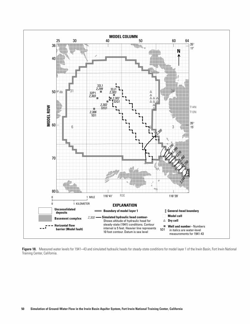
Figure 18. Measured water levels for 1941–43 and simulated hydraulic heads for steady-state conditions for model layer 1 of the Irwin Basin, Fort Irwin National Training Center, California.
25 30 40 50 6036
40
50
60
70
80
64MODEL COLUMN
MO
DEL
ROW
2,302
2,303
2,302
2,303
2,306
2,299
2,302
2,303
2,302
2,303
2,306
2,299
2,300
2,290
2,280
2,270
2,260
2,250
2,240
5D1
32Q1
32Q1
32L132J1
32P1
35°15'
116°39'116°41'
35°17'
N
Model cellDry cell
Well and number - Numbersin italics are water-levelmeasurements for 1941-43
EXPLANATION
Simulated hydraulic head contour-Shows altitude of hydraulic head forsteady-state (1941) conditions. Contourinterval is 5 feet. Heavier line represents10 foot contour. Datum is sea level
Boundary of model layer 1 General-head boundary
0
0 1 KILOMETER
1 MILE
2,300
Horizontal flowbarrier (Model fault)
6
31
3
34
T14NT13N
R3E
5D1
Basement complex
Unconsolidateddeposits
50 Simulation of Ground-Water Flow in the Irwin Basin Aquifer System, Fort Irwin National Training Center, California
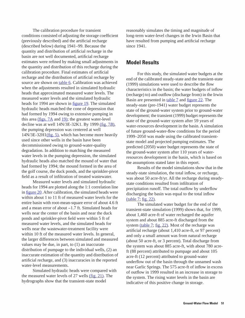
The calibration procedure for transient conditions consisted of adjusting the storage coefficient (previously described) and the artificial recharge (described below) during 1941–99. Because the quantity and distribution of artificial recharge in the basin are not well documented, artificial recharge estimates were refined by making small adjustments in the quantity and distribution of this recharge during the calibration procedure. Final estimates of artificial recharge and the distribution of artificial recharge by source are shown on table 6. Calibration was achieved when the adjustments resulted in simulated hydraulic heads that approximated measured water levels. The measured water levels and the simulated hydraulic heads for 1994 are shown in figure 19. The simulated hydraulic heads matched the cone of depression that had formed by 1994 owing to extensive pumping in this area (figs. 7A and 19); the greatest water-level decline was at well 14N/3E-32K1. By 1999 (fig. 7B), the pumping depression was centered at well 14N/3E-32H1(fig. 5), which has become more heavily used since other wells in the basin have been decommissioned owing to ground-water-quality degradation. In addition to matching the measured water levels in the pumping depression, the simulated hydraulic heads also matched the mound of water that had formed by 1994; the mound formed in the area of the golf course, the duck ponds, and the sprinkler-pivot field as a result of infiltration of treated wastewater.
Measured water levels and simulated hydraulic heads for 1994 are plotted along the 1:1 correlation line in figure 20. After calibration, the simulated heads were within about 1 to 11 ft of measured water levels for the entire basin with root-mean-square error of about 4.6 ft and a mean error of about −1.7 ft. Simulated heads for wells near the center of the basin and near the duck ponds and sprinkler-pivot field were within 5 ft of measured water levels, and the simulated heads for wells near the wastewater-treatment facility were within 10 ft of the measured water levels. In general, the larger differences between simulated and measured values may be due, in part, to (1) an inaccurate distribution of pumpage to the individual wells, (2) an inaccurate estimation of the quantity and distribution of artificial recharge, and (3) inaccuracies in the reported water-level measurements.
Simulated hydraulic heads were compared with the measured water levels of 27 wells (fig. 21). The hydrographs show that the transient-state model
reasonably simulates the timing and magnitude of long-term water-level changes in the Irwin Basin that have resulted from pumping and artificial recharge since 1941.
Model Results
For this study, the simulated water budgets at the end of the calibrated steady-state and the transient-state (1999) simulations were used to describe the flow characteristics in the basin; the water budgets of inflow (recharge) to) and outflow (discharge from) in the Irwin Basin are presented in table 7 and figure 22. The steady-state (pre-1941) water budget represents the state of the ground-water system prior to ground-water development; the transient (1999) budget represents the state of the ground-water system after 59 years of water-resources development in the basin. A simulation of future ground-water-flow conditions for the period 1999–2050 was made using the calibrated transient-state model and projected pumping estimates. The predicted (2050) water budget represents the state of the ground-water system after 110 years of water-resources development in the basin, which is based on the assumptions stated later in this report.
Results of the model simulations show that in the steady-state simulation, the total inflow, or recharge, was about 50 acre-ft/yr. All the recharge during steady-state conditions resulted from infiltration of precipitation runoff. The total outflow by underflow discharging the basin was equal to the total inflow (table 7; fig. 22).
The simulated water budget for the end of the transient-state simulation (1999) shows that, for 1999, about 1,460 acre-ft of water recharged the aquifer system and about 885 acre-ft discharged from the system (table 7; fig. 22). Most of the recharge was artificial recharge (about 1,410 acre-ft, or 97 percent) and only a small amount was from natural recharge (about 50 acre-ft, or 3 percent). Total discharge from the system was about 885 acre-ft, with about 780 acre-ft (88 percent) attributed to pumpage and about 105 acre-ft (12 percent) attributed to ground-water underflow out of the basin through the unnamed wash near Garlic Springs. The 575 acre-ft of inflow in excess of outflow in 1999 resulted in an increase in storage to the system. The rising water levels in the basin are indicative of this positive change in storage.
Ground-Water Flow Model 51
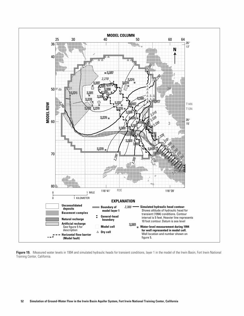
Figure 19. Measured water levels in 1994 and simulated hydraulic heads for transient conditions, layer 1 in the model of the Irwin Basin, Fort Irwin National Training Center, California.
Horizontal flow barrier(Model fault)
Basement complex
Natural rechargeArtificial rechargeSee figure 5 fordescription
Unconsolidateddeposits
25 30 40 50 6036
40
50
60
70
80
64MODEL COLUMN
MO
DEL
ROW
2,270
2,280
2,280
2,290
2,29
0
2,30
0
2,300
2,290
2,310
2,310
2,310
2,320
2,330
2,320
2,270
2,280
2,280
2,290
2,29
0
2,30
0
2,300
2,290
2,280
2,280
2,270
2,270
2,260
2,260
2,250
2,250
2,310
2,310
2,310
2,320
2,330
2,320
2,267
2,267
2,274 2,281
2,276
2,272 2,270
2,273
2,276
2,2632,268
2,2692,271
2,2762,274
2,277
2,278
2,286
2,2962,306
2,3162,312
2,309
2,2902,308
2,286
2,283
2,287
2,2932,317
2,266
2,267
2,267
2,274 2,281
2,276
2,272 2,270
2,273
2,276
2,2632,268
2,2692,271
2,2762,274
2,277
2,278
2,286
2,2962,306
2,3162,312
2,309
2,2902,308
2,286
2,283
2,287
2,2932,317
2,266
35°15'
116°39'116°41'
35°17'
N
Model cell
Dry cell
Water-level measurement during 1994for well represented in model cell.Well location and number shown onfigure 5.
EXPLANATIONBoundary of
model layer 1
General-headboundary
0
0 1 KILOMETER
1 MILE
2,300
6
31
3
34
T14NT13N
R3E
2,2962,296
Simulated hydraulic head contour-Shows altitude of hydraulic head fortransient (1994) conditions. Contourinterval is 5 feet. Heavier line represents10 foot contour. Datum is sea level
52 Simulation of Ground-Water Flow in the Irwin Basin Aquifer System, Fort Irwin National Training Center, California
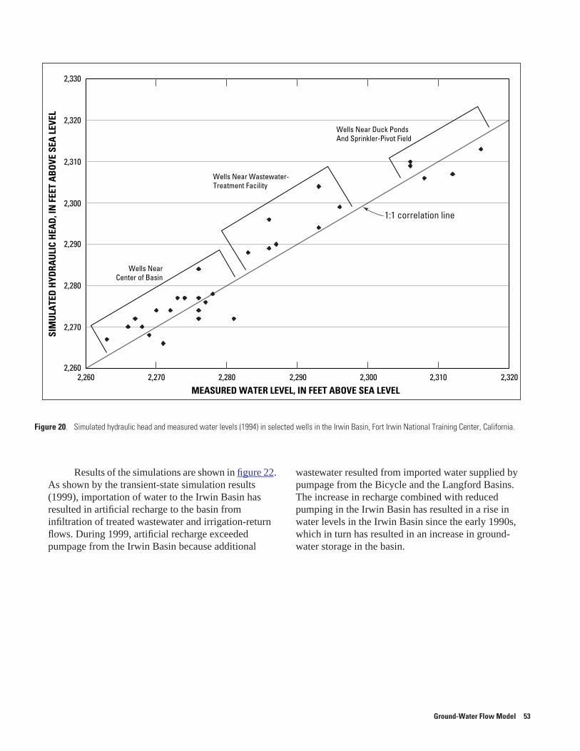
Results of the simulations are shown in figure 22. As shown by the transient-state simulation results (1999), importation of water to the Irwin Basin has resulted in artificial recharge to the basin from infiltration of treated wastewater and irrigation-return flows. During 1999, artificial recharge exceeded pumpage from the Irwin Basin because additional
wastewater resulted from imported water supplied by pumpage from the Bicycle and the Langford Basins. The increase in recharge combined with reduced pumping in the Irwin Basin has resulted in a rise in water levels in the Irwin Basin since the early 1990s, which in turn has resulted in an increase in ground-water storage in the basin.
Figure 20. Simulated hydraulic head and measured water levels (1994) in selected wells in the Irwin Basin, Fort Irwin National Training Center, California.
2,260
2,270
2,280
2,290
2,300
2,310
2,320
2,330
2,260 2,270 2,280 2,290 2,300 2,310 2,320
MEASURED WATER LEVEL, IN FEET ABOVE SEA LEVEL
SIM
ULA
TED
HYD
RAU
LIC
HEA
D,I
NFE
ETA
BO
VESE
ALE
VEL
Wells NearCenter of Basin
Wells Near Wastewater-Treatment Facility
Wells Near Duck PondsAnd Sprinkler-Pivot Field
1:1 correlation line
Ground-Water Flow Model 53
Figure 21. Measured water levels and simulated hydraulic heads for selected wells in the Irwin Basin, Fort Irwin National Training Center, California. A, 1941–99. B, 1980–99. and C, 1990–99.
Layer 1Layer 2
Simulated -
14N/3E-32P414N/3E-32P114N/3E-32M1
Measured -
13N/3E-5D114N/3E-32N3
Measured -
14N/3E-32Q114N/3E-32K6
Measured - Measured -14N/3E-32H114N/3E-32K6
14N/3E-32K614N/3E-32J1
Measured -
14N/3E-32K614N/3E-32K1
Measured -
2,320
2,300
2,280
2,260
2,240
2,320
2,300
2,280
2,260
2,240
2,320
WA
TER
-LEV
ELA
LTIT
UD
E,IN
FEET
AB
OV
ES
EALE
VEL
2,300
2,280
2,260
2,240
A
1940 19601950
YEAR1970 1980 1990 2000 1940 19601950 1970 1980 1990 2000
YEAR
54 Simulation of Ground-Water Flow in the Irwin Basin Aquifer System, Fort Irwin National Training Center, California
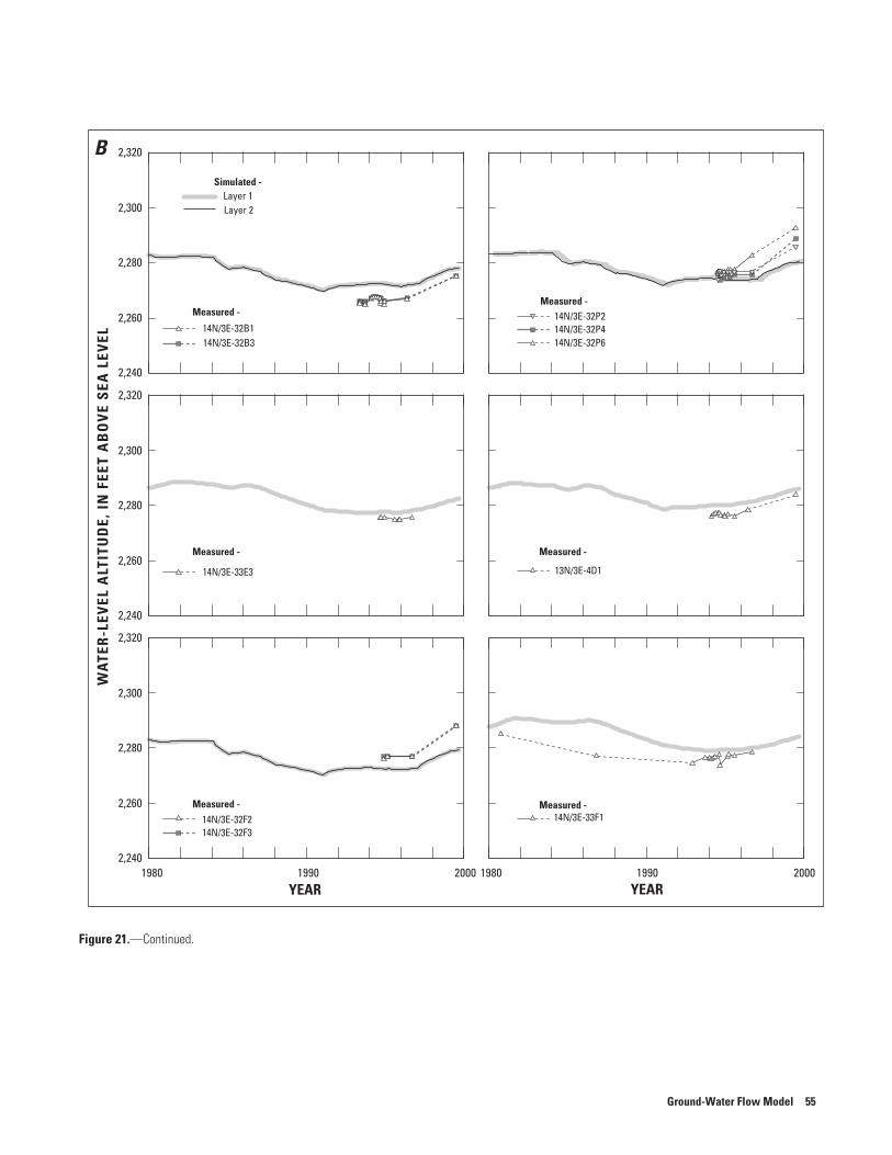
Figure 21.—Continued.
Layer 1Layer 2
Simulated -
14N/3E-32B1
14N/3E-33E3 13N/3E-4D1
14N/3E-33F114N/3E-32F214N/3E-32F3
14N/3E-32B3
Measured -
Measured - Measured -
Measured -Measured -
Measured -14N/3E-32P214N/3E-32P414N/3E-32P6
2,320
2,300
2,280
2,260
2,240
2,320
2,300
2,280
2,260
2,240
2,320
WA
TER
-LEV
ELA
LTIT
UD
E,IN
FEET
AB
OV
ES
EALE
VEL
2,300
2,280
2,260
2,240
B
1980YEAR
1990 2000 1980 1990 2000YEAR
Ground-Water Flow Model 55
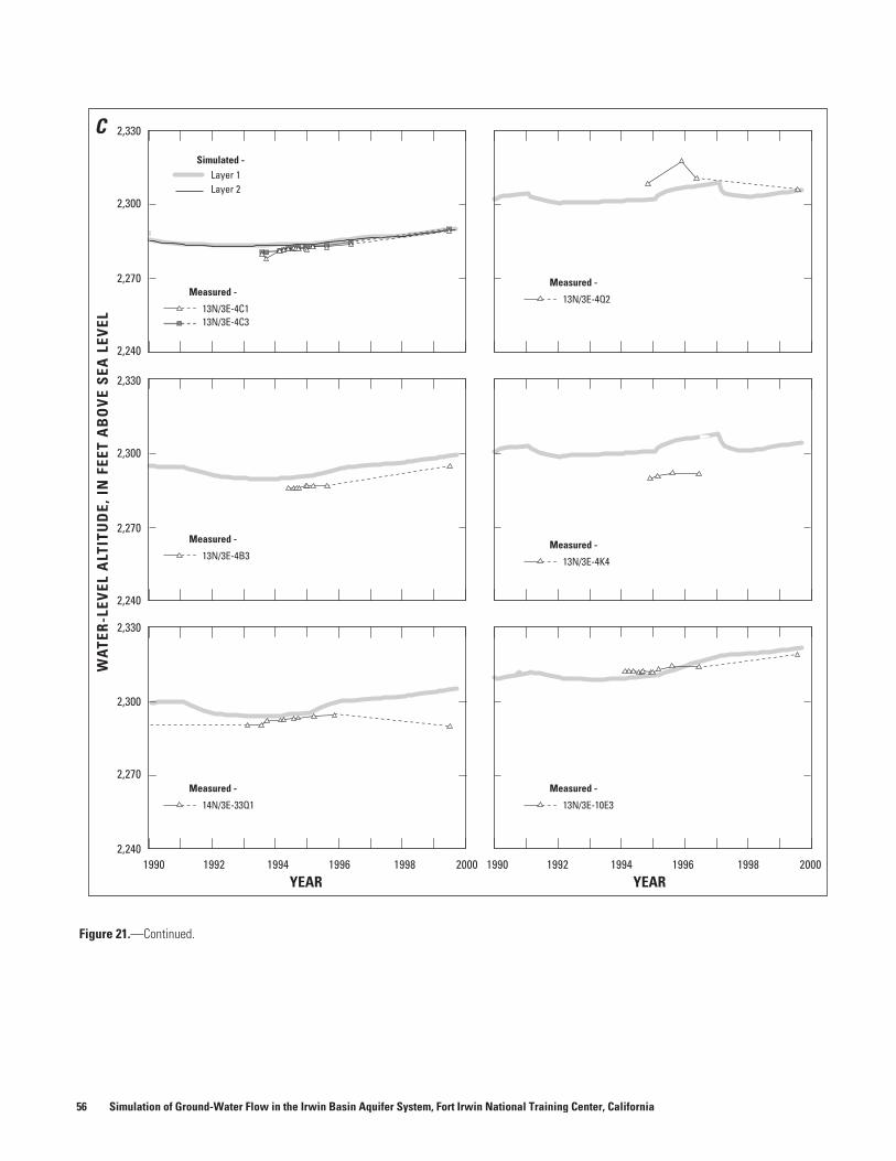
Figure 21.—Continued.
Layer 1Layer 2
Simulated -
13N/3E-4C1
13N/3E-4B3
14N/3E-33Q1
13N/3E-4C3
Measured -
Measured -
Measured -
13N/3E-10E3
Measured -
13N/3E-4K4
Measured -
13N/3E-4Q2
Measured -
WA
TER
-LEV
ELA
LTIT
UD
E,IN
FEET
AB
OV
ES
EALE
VEL
2,330
2,300
2,270
2,240
2,330
2,300
2,270
2,240
YEAR1990 1992 1994 1996 1998 2000
YEAR1990 1992 1994 1996 1998 2000
2,330
2,300
2,270
2,240
C
56 Simulation of Ground-Water Flow in the Irwin Basin Aquifer System, Fort Irwin National Training Center, California
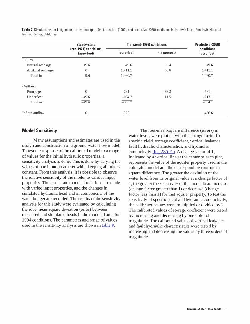
Table 7. Simulated water budgets for steady-state (pre-1941), transient (1999), and predictive (2050) conditions in the Irwin Basin, Fort Irwin National Training Center, California
Steady-state(pre-1941) conditions
(acre-feet)
Transient (1999) conditions Predictive (2050) conditions(acre-feet)(acre-feet) (in percent)
Inflow:
Natural recharge 49.6 49.6 3.4 49.6
Artificial recharge 0 1,411.1 96.6 1,411.1
Total in 49.6 1,460.7 1,460.7
Outflow:
Pumpage 0 –781 88.2 –781
Underflow –49.6 –104.7 11.5 –213.1
Total out –49.6 –885.7 –994.1
Inflow-outflow 0 575 466.6
Model Sensitivity
Many assumptions and estimates are used in the design and construction of a ground-water flow model. To test the response of the calibrated model to a range of values for the initial hydraulic properties, a sensitivity analysis is done. This is done by varying the values of one input parameter while keeping all others constant. From this analysis, it is possible to observe the relative sensitivity of the model to various input properties. Thus, separate model simulations are made with varied input properties, and the changes in simulated hydraulic head and in components of the water budget are recorded. The results of the sensitivity analysis for this study were evaluated by calculating the root-mean-square deviation (error) between measured and simulated heads in the modeled area for 1994 conditions. The parameters and range of values used in the sensitivity analysis are shown in table 8.
The root-mean-square difference (errors) in water levels were plotted with the change factor for specific yield, storage coefficient, vertical leakance, fault hydraulic characteristics, and hydraulic conductivity (fig. 23A–C). A change factor of 1, indicated by a vertical line at the center of each plot, represents the value of the aquifer property used in the calibrated model and the corresponding root-mean-square difference. The greater the deviation of the water level from its original value at a change factor of 1, the greater the sensitivity of the model to an increase (change factor greater than 1) or decrease (change factor less than 1) for that aquifer property. To test the sensitivity of specific yield and hydraulic conductivity, the calibrated values were multiplied or divided by 2. The calibrated values of storage coefficient were tested by increasing and decreasing by one order of magnitude. The calibrated values of vertical leakance and fault hydraulic characteristics were tested by increasing and decreasing the values by three orders of magnitude.
Ground-Water Flow Model 57
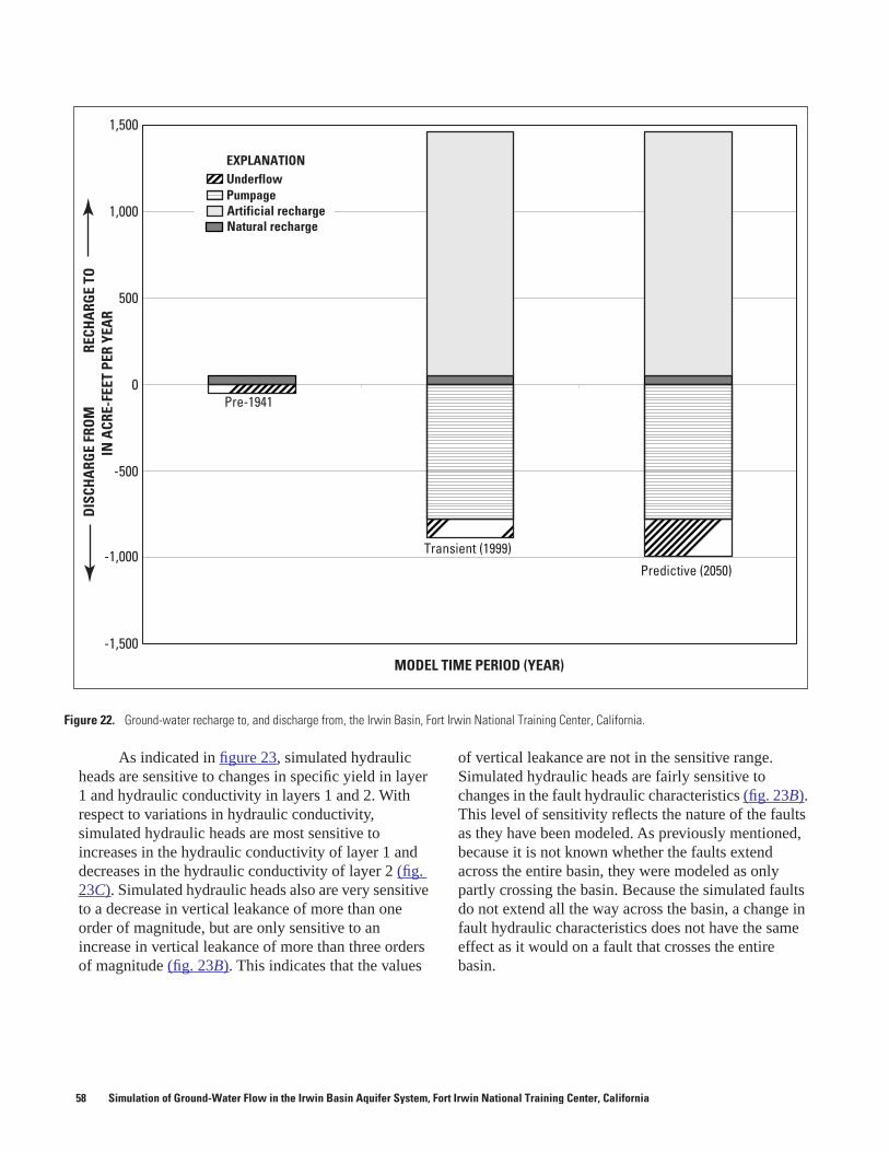
Figure 22. Ground-water recharge to, and discharge from, the Irwin Basin, Fort Irwin National Training Center, California.
Pre-1941
Transient (1999)
Predictive (2050)
MODEL TIME PERIOD (YEAR)
UnderflowEXPLANATION
PumpageArtificial rechargeNatural recharge
-1,000
-1,500
-500
0
500
1,000
1,500
DIS
CHA
RGE
FRO
MRE
CHA
RGE
TOIN
ACR
E-FE
ETPE
RYE
AR
As indicated in figure 23, simulated hydraulic heads are sensitive to changes in specific yield in layer 1 and hydraulic conductivity in layers 1 and 2. With respect to variations in hydraulic conductivity, simulated hydraulic heads are most sensitive to increases in the hydraulic conductivity of layer 1 and decreases in the hydraulic conductivity of layer 2 (fig. 23C). Simulated hydraulic heads also are very sensitive to a decrease in vertical leakance of more than one order of magnitude, but are only sensitive to an increase in vertical leakance of more than three orders of magnitude (fig. 23B). This indicates that the values
of vertical leakance are not in the sensitive range. Simulated hydraulic heads are fairly sensitive to changes in the fault hydraulic characteristics (fig. 23B). This level of sensitivity reflects the nature of the faults as they have been modeled. As previously mentioned, because it is not known whether the faults extend across the entire basin, they were modeled as only partly crossing the basin. Because the simulated faults do not extend all the way across the basin, a change in fault hydraulic characteristics does not have the same effect as it would on a fault that crosses the entire basin.
58 Simulation of Ground-Water Flow in the Irwin Basin Aquifer System, Fort Irwin National Training Center, California
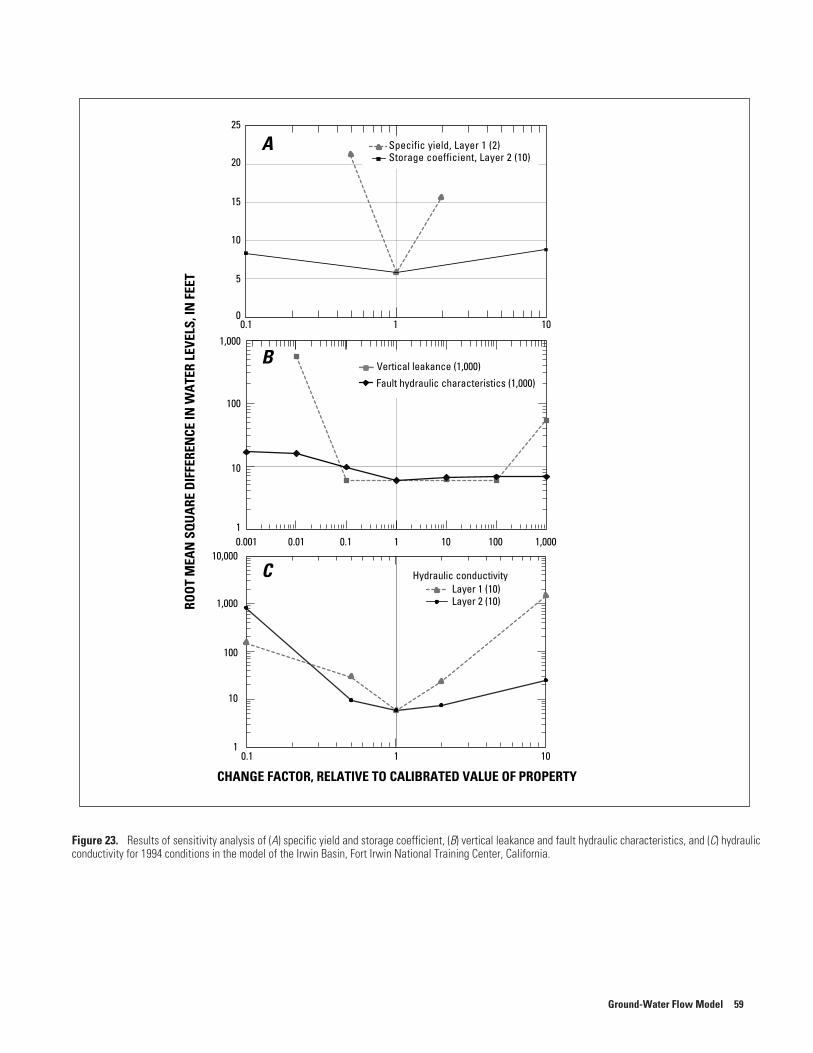
Ground-Water Flow Model 59
Figure 23. Results of sensitivity analysis of (A) specific yield and storage coefficient, (B) vertical leakance and fault hydraulic characteristics, and (C) hydraulic conductivity for 1994 conditions in the model of the Irwin Basin, Fort Irwin National Training Center, California.
0
5
10
15
20
25
0.1 1 10
ROO
TM
EAN
SQU
ARE
DIF
FERE
NCE
INW
ATE
RLE
VELS
,IN
FEET
1
1
10
100
1,000
10,000
10
1,000
100
0.001 0.01 0.1 1 10 100 1,000
0.1 1 10
CHANGE FACTOR, RELATIVE TO CALIBRATED VALUE OF PROPERTY
Hydraulic conductivityLayer 1 (10)Layer 2 (10)
Vertical leakance (1,000)
Fault hydraulic characteristics (1,000)
A
B
C
Specific yield, Layer 1 (2)Storage coefficient, Layer 2 (10)
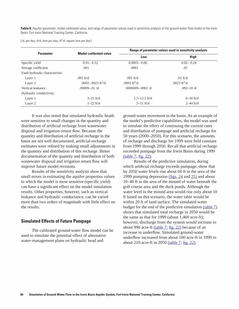
Table 8. Aquifer parameter, model-calibrated value, and range of parameter values used in sensitivity analysis of the ground-water flow model of the Irwin Basin, Fort Irwin National Training Center, California
[/d, per day; ft/d, foot per day; ft2/d, square foot per day]
Parameter Model-calibrated valueRange of parameter values used in sensitivity analysis
Low High
Specific yield 0.01– 0.12 0.0005– 0.06 0.02– 0.24
Storage coefficient .001 .0001 .01
Fault hydraulic characteristic
Layer 1 .001 ft/d .001 ft/d .01 ft/d
Layer 2 .0002–.0023 ft2/d .0002 ft2/d .0023 ft2/d
Vertical leakance .00009–.01 /d .0000009–.0001 /d .092–10 /d
Hydraulic conductivity:
Layer 1 3–25 ft/d 1.5–12.5 ft/d 6–50 ft/d
Layer 2 1–22 ft/d .5–11 ft/d 2–44 ft/d
It was also noted that simulated hydraulic heads were sensitive to small changes in the quantity and distribution of artificial recharge from wastewater disposal and irrigation-return flow. Because the quantity and distribution of artificial recharge in the basin are not well documented, artificial-recharge estimates were refined by making small adjustments in the quantity and distribution of this recharge. Better documentation of the quantity and distribution of both wastewater disposal and irrigation return flow will improve future model revisions.
Results of the sensitivity analysis show that small errors in estimating the aquifer properties values to which the model is most sensitive (specific yield) can have a significant effect on the model simulation results. Other properties, however, such as vertical leakance and hydraulic conductance, can be varied more than two orders of magnitude with little effect on the results.
Simulated Effects of Future Pumpage
The calibrated ground-water flow model can be used to simulate the potential effect of alternative water-management plans on hydraulic head and
ground-water movement in the basin. As an example of the model’s predictive capabilities, the model was used to simulate the effect of continuing the current rates and distribution of pumpage and artificial recharge for 50 years (2000–2050). For this scenario, the amounts of recharge and discharge for 1999 were held constant from 1999 through 2050. Recall that artificial recharge exceeded pumpage from the Irwin Basin during 1999 (table 7; fig. 22).
Results of the predictive simulation, during which artificial recharge exceeds pumpage, show that by 2050 water levels rise about 60 ft in the area of the 1999 pumping depression (figs. 24 and 25) and about 10–40 ft in the area of the mound of water beneath the golf course area and the duck ponds. Although the water level in the mound area would rise only about 10 ft based on this scenario, the water table would be within 20 ft of land surface. The simulated water budget for the end of the predictive simulation (table 7) shows that simulated total recharge in 2050 would be the same as that for 1999 (about 1,460 acre-ft); however, discharge from the system would increase to about 990 acre-ft (table 7; fig. 22) because of an increase in underflow. Simulated ground-water underflow increased from about 100 acre-ft in 1999 to about 210 acre-ft in 2050 (table 7; fig. 22).
60 Simulation of Ground-Water Flow in the Irwin Basin Aquifer System, Fort Irwin National Training Center, California
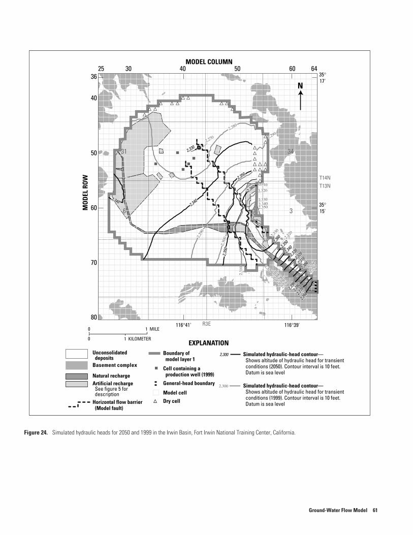
Figure 24. Simulated hydraulic heads for 2050 and 1999 in the Irwin Basin, Fort Irwin National Training Center, California.
25 30 40 50 6036
40
50
60
70
80
64MODEL COLUMN
MO
DEL
ROW
2,2802,280
2,2902,290
2,29
02,
290
2,30
02,
300
2,3102,310
2,3202,320
2,3302,330
2,330
2,330
2,3402,3402,3502,350
2,31
02,
310 2,320
2,320
2,320
2,320
2,310
2,310
2,300
2,300
2,290
2,290
2,280
2,280
2,270
2,270
2,260
2,260
2,250
2,250
2,2702,270
2,260
2,2602,2
702,2
702,280
2,2802,290
2,290
2,3302,330
2,3402,340
2,3502,350
2,35
02,
350 2,350
2,350
2,340
2,340
2,330
2,330
2,320
2,320
2,310
2,310
2,300
2,300
2,3402,340
2,3602,360
2,360
2,360
35°15'
116°39'116°41'
35°17'
N
6
31
3
34
Model cell
Dry cell
Cell containing aproduction well (1999)
EXPLANATION
Simulated hydraulic-head contour—Shows altitude of hydraulic head for transientconditions (2050). Contour interval is 10 feet.Datum is sea level
Simulated hydraulic-head contour—Shows altitude of hydraulic head for transientconditions (1999). Contour interval is 10 feet.Datum is sea level
Boundary ofmodel layer 1
General-head boundary
2,300
2,300
T14NT13N
R3E0
0 1 KILOMETER
1 MILE
Horizontal flow barrier(Model fault)
Basement complex
Natural rechargeArtificial rechargeSee figure 5 fordescription
Unconsolidateddeposits
Ground-Water Flow Model 61
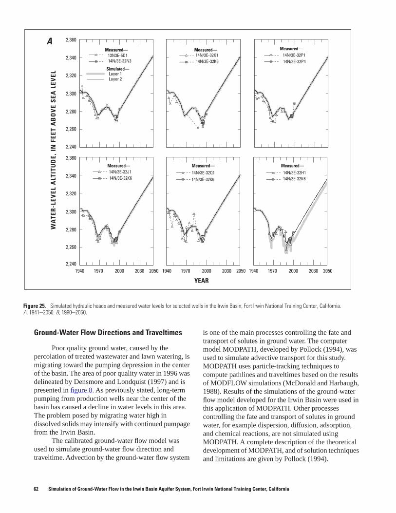
Ground-Water Flow Directions and Traveltimes
Poor quality ground water, caused by the percolation of treated wastewater and lawn watering, is migrating toward the pumping depression in the center of the basin. The area of poor quality water in 1996 was delineated by Densmore and Londquist (1997) and is presented in figure 8. As previously stated, long-term pumping from production wells near the center of the basin has caused a decline in water levels in this area. The problem posed by migrating water high in dissolved solids may intensify with continued pumpage from the Irwin Basin.
The calibrated ground-water flow model was used to simulate ground-water flow direction and traveltime. Advection by the ground-water flow system
is one of the main processes controlling the fate and transport of solutes in ground water. The computer model MODPATH, developed by Pollock (1994), was used to simulate advective transport for this study. MODPATH uses particle-tracking techniques to compute pathlines and traveltimes based on the results of MODFLOW simulations (McDonald and Harbaugh, 1988). Results of the simulations of the ground-water flow model developed for the Irwin Basin were used in this application of MODPATH. Other processes controlling the fate and transport of solutes in ground water, for example dispersion, diffusion, adsorption, and chemical reactions, are not simulated using MODPATH. A complete description of the theoretical development of MODPATH, and of solution techniques and limitations are given by Pollock (1994).
Figure 25. Simulated hydraulic heads and measured water levels for selected wells in the Irwin Basin, Fort Irwin National Training Center, California. A, 1941–2050. B, 1990–2050.
Simulated—Layer 1Layer 2
14N/3E-32P114N/3E-32P4
14N/3E-32J114N/3E-32K6
14N/3E-32K114N/3E-32K6
13N3E-5D114N/3E-32N3
Measured—Measured— Measured—
14N/3E-32K614N/3E-32Q1
14N/3E-32K614N/3E-32H1
WA
TER
-LEV
ELA
LTIT
UD
E,IN
FEET
AB
OV
ES
EALE
VEL
A
1940 1970 2000 2030
YEAR
2050 1940 1970 2000 2030 2050 1940 1970 2000 2030 2050
2,360
2,340
2,320
2,300
2,280
2,260
2,240
2,360
2,340
2,320
2,300
2,280
2,260
2,240
Measured— Measured—Measured—
62 Simulation of Ground-Water Flow in the Irwin Basin Aquifer System, Fort Irwin National Training Center, California
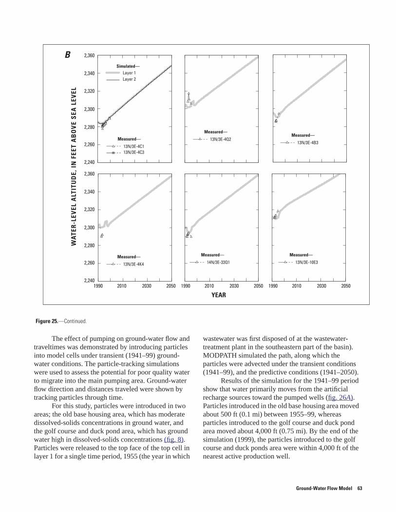
The effect of pumping on ground-water flow and traveltimes was demonstrated by introducing particles into model cells under transient (1941–99) ground-water conditions. The particle-tracking simulations were used to assess the potential for poor quality water to migrate into the main pumping area. Ground-water flow direction and distances traveled were shown by tracking particles through time.
For this study, particles were introduced in two areas; the old base housing area, which has moderate dissolved-solids concentrations in ground water, and the golf course and duck pond area, which has ground water high in dissolved-solids concentrations (fig. 8). Particles were released to the top face of the top cell in layer 1 for a single time period, 1955 (the year in which
wastewater was first disposed of at the wastewater-treatment plant in the southeastern part of the basin). MODPATH simulated the path, along which the particles were advected under the transient conditions (1941–99), and the predictive conditions (1941–2050).
Results of the simulation for the 1941–99 period show that water primarily moves from the artificial recharge sources toward the pumped wells (fig. 26A). Particles introduced in the old base housing area moved about 500 ft (0.1 mi) between 1955–99, whereas particles introduced to the golf course and duck pond area moved about 4,000 ft (0.75 mi). By the end of the simulation (1999), the particles introduced to the golf course and duck ponds area were within 4,000 ft of the nearest active production well.
Figure 25.—Continued.
Layer 1Layer 2
Simulated—
13N/3E-4C113N/3E-4C3
Measured— 13N/3E-4Q2
Measured—
13N/3E-4B3
Measured—
13N/3E-4K4
Measured—14N/3E-33Q1
Measured—
13N/3E-10E3
Measured—
WA
TER
-LEV
ELA
LTIT
UD
E,IN
FEET
AB
OV
ES
EALE
VEL
B
YEAR1990 2010 2030 2050 1990 2010 2030 2050 1990 2010 2030 2050
2,360
2,340
2,320
2,300
2,280
2,260
2,240
2,360
2,340
2,320
2,300
2,280
2,260
2,240
Ground-Water Flow Model 63
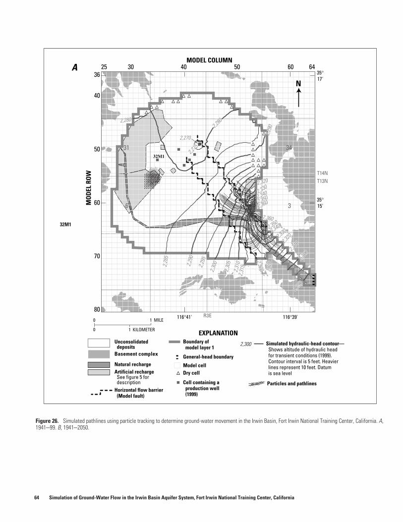
Figure 26. Simulated pathlines using particle tracking to determine ground-water movement in the Irwin Basin, Fort Irwin National Training Center, California. A, 1941–99. B, 1941–2050.
25 30 40 50 6036
40
50
60
70
80
64MODEL COLUMN
MO
DEL
ROW
A
Horizontal flow barrier(Model fault)
Basement complex
Natural rechargeArtificial rechargeSee figure 5 fordescription
Unconsolidateddeposits
2,29
0
2,29
5
2,30
02,29
02,340
2,3602,350
2,28
5
2,330
2,280
2,275
2,270
2,280
2,30
52,
310
2,31
5
2,3202,325
2,290
2,300
2,310
2,320
2,320
2,360
2,3302,3402,350
2,29
0
2,29
5
2,30
02,29
02,340
2,3602,350
2,28
5
2,330
2,280
2,275
2,270
2,280
2,30
52,
310
2,31
5
2,3202,325
2,290
2,300
2,310
2,320
2,320
2,360
2,3302,3402,350
35°15'
116°39'116°41'
35°17'
N
6
31
3
34
T14N
R3E
T13N
Model cellDry cell
Cell containing aproduction well(1999)
EXPLANATIONBoundary of
model layer 1
General-head boundary
2,300
0
0 1 KILOMETER
1 MILE
Particles and pathlines
Simulated hydraulic-head contour—Shows altitude of hydraulic headfor transient conditions (1999).Contour interval is 5 feet. Heavierlines represent 10 feet. Datumis sea level
32M1
32M1
64 Simulation of Ground-Water Flow in the Irwin Basin Aquifer System, Fort Irwin National Training Center, California
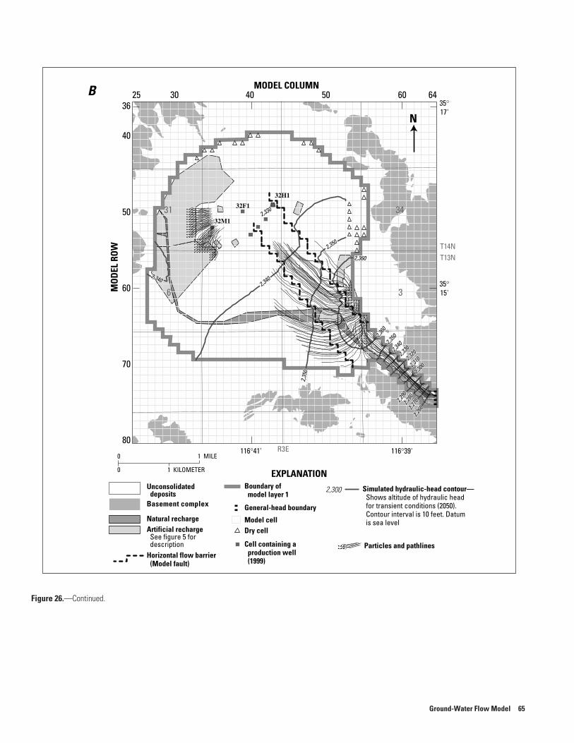
Figure 26.—Continued.
25 30 40 50 6036
40
50
60
70
80
64MODEL COLUMN
MO
DEL
ROW
2,260
2,2602,2
702,2
702,280
2,2802,290
2,290
2,3302,330
2,3402,340
2,3502,350
2,35
02,
350
2,350
2,350
2,340
2,340
2,330
2,330
2,320
2,320
2,310
2,310
2,300
2,300
2,3402,340
2,3602,360
2,360
2,360
35°15'
116°39'116°41'
35°17'
N
6
31
3
34
EXPLANATION
0
0 1 KILOMETER
1 MILE
B
T14NT13N
R3E
Model cellDry cell
Cell containing aproduction well(1999)
Boundary ofmodel layer 1
General-head boundary
2,300
Horizontal flow barrier(Model fault)
Basement complex
Natural rechargeArtificial rechargeSee figure 5 fordescription
Unconsolidateddeposits
Particles and pathlines
Simulated hydraulic-head contour—Shows altitude of hydraulic headfor transient conditions (2050).Contour interval is 10 feet. Datumis sea level
32F1
32H1
32M1
Ground-Water Flow Model 65
Results of the simulation for the 1941–2050 period show that by 2050 most of the particles introduced in the old base housing area in 1955 will have moved about 1,200 ft (0.25 mi), reaching the nearest well (14N/3E-32M1, believed to have last been pumped in 1996) (fig. 26B). Particles from the area of the golf course and duck ponds will have moved more than 5,500 ft (1 mi) toward pumped wells 14N/3E-32H1 and -32J1 in the northcentral part of the basin. These results indicate that with continued pumping the high dissolved-solids and nitrate water will eventually reach the production wells.
One significant limitation to using the particle-tracking results to determine ground-water pathlines and traveltimes is that the pathlines for instantaneous releases were calculated using the assumption that the particles were introduced into the system in 1955 when the first wastewater-treatment facility was built. Therefore, the pathlines generated by MODPATH for the base housing area, which was not built until the early 1960s, indicate that the particles have traveled farther than they actually would have.
Limitations of the Model
A numerical model is useful for testing and refining a conceptual model of a ground-water flow system, developing an understanding of the system, guiding data collection, and projecting aquifer responses to changes in aquifer stresses within specified limits. However, a model can only approximate the actual system and is based on simplified assumptions and on average and estimated conditions. Thus, the results of model simulations are only as accurate as the measured or estimated data used to constrain the simulations.
One limitation of this model for predicting aquifer responses to changes in aquifer stresses is due to early pumpage distribution among the wells, which may be inaccurate because distribution records prior to 1990 are not available. Another limitation of the model is that the artificial recharge estimates may be inaccurate because historical records on the quantities of water used for irrigation and discharged from the wastewater-treatment facility were not available. The data for these two sources, therefore, were estimated from pumpage data. Because the model was used to test different quantities and distributions of artificial recharge, the artificial recharge estimates were as
representative as possible considering the data limitations. However, more accurate estimates of artificial recharge quantities and distribution could be used to update and verify the model as they become available.
This model is an approximation of the alluvial aquifer system of the Irwin Basin and, thus, it simulates responses of the ground-water flow system to recharge to and discharge from the alluvial aquifer system. Although the landfill area is included in the modeled area, the landfill area was modeled as a thin alluvial aquifer in this part of the basin and does not include the underlying fractured aquifer system which most likely occurs in the landfill area.
SUMMARY AND CONCLUSIONS
Ground-water pumping in the Irwin Basin underlying the Fort Irwin National Training Center (NTC), California resulted in water-level declines of about 30 ft in the central part of the basin between 1941 and 1996. Since 1996, pumpage from the Irwin Basin has decreased, but the decrease has been offset by an increase in pumpage in the Bicycle and the Langford Basins that is imported to the Irwin Basin. Artificial recharge from wastewater-effluent infiltration and irrigation-return flow stabilized water levels in the early 1990’s; but there is concern that future water demands associated with expansion of the base may cause water-level declines in the more heavily pumped basins. To address these concerns, a ground-water flow model of the Irwin Basin was developed to better understand the aquifer system, assess the long-term availability and quality of ground water, evaluate ground-water conditions owing to current pumping, and to plan for future water needs at the base.
The Fort Irwin NTC, located about 130 mi northeast of Los Angeles in the northern part of the Mojave Desert, encompasses several ground-water basins. The Irwin Basin is one of three basins currently supplying ground water to the base. The Irwin Basin has a fairly flat floor and is bounded, for the most part, by rugged mountainous terrain. There are no perennial streams in the basin, but several dry washes indicate that there is some surface flow during, or immediately after, large storms. The climate of the Irwin Basin consists of scant precipitation, hot summers, and cool winters.
66 Simulation of Ground-Water Flow in the Irwin Basin Aquifer System, Fort Irwin National Training Center, California
The Irwin Basin is filled with as much as 950 ft of unconsolidated deposits that consist of younger alluvium of Quaternary age and older alluvium of late Tertiary to Quaternary age. These deposits are underlain by volcanic rocks of late Tertiary to Quaternary age and igneous and metamorphic rocks of pre-Tertiary age, which do not contain significant water-bearing units except in areas where they are jointed and fractured.
The aquifer system in the Irwin Basin consists of an upper aquifer and a lower aquifer. The upper aquifer is unconfined and is contained within the saturated part of the younger alluvium. The lower aquifer is confined throughout most of the basin and includes the older alluvium. The effective base of the ground-water system is the top of the unweathered basement complex. Several faults cross the Irwin Basin and act as partial barriers to ground-water flow. Under predevelopment conditions, ground water discharged from the basin as underflow beneath the unnamed wash near Garlic Spring to the Langford Basin.
Natural recharge occurs only by infiltration of precipitation runoff during and shortly after high-intensity or long-duration storms, and most of the recharge probably occurs along the normally dry washes. During a previous study, average annual recharge to the Irwin Basin was estimated at about 150 acre-ft/yr for 1941–51. However, recent data indicate that little present-day precipitation reaches the water table. Thus, recharge from precipitation runoff is estimated to be less than 150 acre-ft/yr. Natural discharge is by subsurface underflow beneath the wash near Garlic Spring.
Ground-water pumping in the Irwin Basin began in 1941; pumpage from the basin has ranged from 30 to 1,927 acre-ft/yr. Fort Irwin began receiving additional ground water pumped from the Bicycle Basin in 1967 and from the Langford Basin in 1992. Most of the water that is not consumed in the Irwin Basin is discharged to a wastewater-collection system and treatment facility. Percolation of wastewater is the largest source of ground-water recharge to the basin. Between 58 and 70 percent of the total pumpage from the three basins delivered to the wastewater-treatment facility between 1941 and 1999 was estimated to recharge the ground-water system. This recharge is
distributed over the base golf course, driving range, and sprinkler-pivot field in the southeastern part of the basin. Since 1996, wastewater disposal in the sprinkler-pivot field has ceased.
A ground-water flow model was developed to better understand the aquifer system and to assess the long-term availability and quality of ground water in the basin. The aquifer system was vertically discretized into two layers representing the upper and lower aquifers, and boundary conditions were determined for the aquifer system. Hydraulic conductivities, altitudes of the layer bottoms, vertical leakance, specific yields, storage coefficients, recharge, and discharge were determined using existing and newly collected geohydrologic data. Rates and distribution of recharge and discharge and aquifer properties were determined from existing data or estimated when and where data were unavailable, and assigned to the model grid.
The model was calibrated using a trial-and-error method in adjusting initial estimates of aquifer properties, recharge, and discharge to get a best match between simulated hydraulic heads and measured water levels, and selected water-budget items. Conditions simulated by the calibrated model of the Irwin Basin reflect measured water levels and show that ground-water levels in the Irwin Basin began to decline in 1941 and stabilized in the early 1990s. There is a pumping depression near the pumped wells and a mound of recharge in the wastewater-treatment facility and disposal area. There have been two periods of recovery in water level since the development of ground water the in Irwin Basin; these periods coincide with a period of decreased pumpage from the Irwin Basin and a period of increased recharge to the Irwin Basin as a result of the importation of ground water from the Bicycle Basin beginning in 1967 and from the Langford Basin beginning in 1992.
Since 1992, however, recharge has exceeded pumpage in the Irwin Basin. Assuming that this trend continues, predictive simulations show that water levels may rise as much as 60 ft by 2050 in the area of the pumping depression, and about 10–40 ft in the wastewater-treatment facility and disposal area. A water-level rise of 10–40 ft in the wastewater-treatment facility area will bring the water table to about 20 ft below land surface by 2050.
Summary and Conclusions 67
In addition to potential problems associated with rising water levels, there is a problem posed by the migration of ground water containing high dissolved-solids concentrations. The high concentrations are caused by the percolation of treated wastewater through evaporite deposits underlying the wastewater-treatment facility and disposal area. The poor quality ground water is migrating from this area toward the pumping depression beneath the main base. This problem was documented during the first phase of this study; the high concentrations can be expected to intensify with continued pumping from the Irwin Basin.
Particle-tracking simulations were used to determine the pathlines and traveltimes of ground water high in dissolved-solids concentrations and to assess its potential migration into the main pumping area. Particles, introduced in two areas where ground water has high-dissolved-solids—the old base housing area and the golf course and duck pond area—were tracked from 1955 to 1999 and 1955 to 2050. Results of the simulations show that water moves from these source areas toward the pumped wells. Particles introduced in the old base housing area in 1955 moved about 500 ft (0.1 mi) by 1999, whereas particles introduced to the golf course and duck pond area in 1955 moved about 4,000 ft (0.75 mi). Particle-tracking to 2050 show that most of the particles in the old base housing area will reach the nearest well, about 1,200 ft (0.25 mi) away, and particles in the area of the golf course and duck pond area will move about 5,500 ft (1 mi), toward pumped wells in the northcentral part of the basin.
SELECTED REFERENCES
C.F. Hostrup and Associates, 1955, Water Resources Survey Camp Irwin, California; 109 p.
Densmore, J.N., and Londquist, C.J., 1997, Ground-water hydrology and water quality of the Irwin Basin at Fort Irwin National Training Center, California: U.S. Geological Survey Water-Resources Investigations Report 97-4092, 159 p.
Driscoll, F.G., 1986, Groundwater and wells: St. Paul, Minnesota, Johnson Division, p. 75.
EarthInfo, Inc., 1995, National Climatic Data Center summary of the day—West 1994: Boulder, Colorado, EarthInfo, Inc. One CD-ROM.
———2000, EarthInfo CD2 reference manual—for all EarthInfo CD-ROM databases: Boulder, Colorado, EarthInfo, Inc.
Fetter, C.W., 1994, Applied Hydrogeology: Englewood Cliffs, New Jersey, Prentice-Hall, p. 116.Heath, R.C., 1983, Basic ground-water hydrology: U.S.
Geological Survey Water- Supply Paper 2220, 84 p.
Hsieh, P.A., and Freckleton, J.R., 1993, Documentation of a computer program to simulate horizontal-flow barriers using the U.S. Geological Survey’s Modular Three-Dimensional Finite-Difference Ground-Water Flow Model: U.S. Geological Survey Open-File Report 92-477, 32 p.
Izbicki, J.A., Radyk, J., and Michel, R.L., 2000, Water movement through a thick unsaturated zone underlying an intermittent stream in the Mojave Desert, southern California, USA: Journal of Hydrology, v. 238, p. 194–217.
James M. Montgomery and Associates, Inc., 1981, Water supply investigation, Fort Irwin, San Bernardino County, California: Phase II Final Report on Ground Water Basin Development and Management.
Kunkel, F., and Riley, F.S., 1959, Geologic reconnaissance and test-well drilling, Camp Irwin, California: U.S. Geological Survey Water-Supply Paper 1460-F, 271 p.
Lohman, S.W., 1972, Ground-water hydraulics: U.S. Geological Survey Professional Paper 708, 70 p.
Londquist, C.J., and Martin, Peter, 1991, Geohydrology and ground-water-flow simulation of the Surprise Spring Basin aquifer system, San Bernardino County, California: U.S. Geological Survey Water-Resources Investigations Report 89-4099, 41 p.
McDonald, M.G., and Harbaugh, A.W., 1988, A modular three-dimensional finite- difference ground-water flow model: Techniques of Water-Resources Investigations of the U.S. Geological Survey, book 6, chap. A1, 576 p.
National Oceanic and Atmospheric Administration, 1994, Climatological data, annual summary, California, 1994: Asheville, North Carolina, National Oceanic and Atmospheric Administration, v. 98, no. 13.
Pollock, D.W., 1994, User’s guide for MODPATH/MODPATH-PLOT, Version 3: A particle tracking post-processing package for MODFLOW, the U.S. Geological Survey finite-difference ground-water flow model: U.S. Geological Survey Open-File Report 94-464, 245 p.
Thomasson, H.G., Jr., Olmsted, F.H., and LeRoux. E.F., 1960, Geology, water resources, and usable ground-water storage capacity of part of Solano County, California: U.S. Geological Survey Water-Supply Paper 1464, 693 p.
68 Simulation of Ground-Water Flow in the Irwin Basin Aquifer System, Fort Irwin National Training Center, California

Wilson F. So and Associates, Inc., 1989, U.S. Army National Training Center at Fort Irwin, California, Water Basin Development Plan, Final Report, June 1989: 85 p.
Yount, J.C., Scherner, E.R., Felger, T.J., Miller, D.M., and Stephens, K.A., 1994, Preliminary geologic map of Fort Irwin Basin, north-central Mojave Desert, California: U.S. Geological Survey Open-File Report 94-173, 25 p.
Selected references 69

70 Simulation of Ground-Water Flow in the Irwin Basin Aquifer System, Fort Irwin National Training Center, California

WRIR
02-4264D
ENSM
ORE
—SIM
ULA
TION
OF
GRO
UN
D-W
ATER
FLOW
INTH
EIRW
INB
ASIN
AQ
UIFER
SYSTEM,
FORT
IRWIN
NA
TION
AL
TRAIN
ING
CENTER,CA
LIFORN
IA
IRWINBASIN
BICYCLEBASIN
LANGFORDBASIN
AquiferSystem
Boundary