SIMULATION OF DIRECT GEOREFERENCING FOR...

International Journal of Remote Sensing and Earth Sciences Vol.14 No.1 June 2017: 71 – 82

@National Institute of Aeronautics and Space of Indonesia (LAPAN) 71

SIMULATION OF DIRECT GEOREFERENCING FOR GEOMETRIC

SYSTEMATIC CORRECTION ON LSA PUSHBROOM IMAGER

Muchammad Soleh1, Wismu Sunarmodo, and Ahmad Maryanto

Remote Sensing Technology and Data Center

Indonesian National Institute of Aeronautics and Space (LAPAN) 1Email: [email protected]

Received: 12 May 2017; Revised: 16 June 2017; Approved: 19 June 2017

Abstract. LAPAN has developed remote sensing data collection by using a pushbroom linescan imager

camera sensor mounted on LSA (Lapan Surveillance Aircraft). The position accuracy and orientation

system for LSA applications are required for Direct Georeferencing and depend on the accuracy of

off-the-shelf integrated GPS/inertial system, which used on the camera sensor. This research aims to

give the accuracy requirement of Inertial Measurement Unit (IMU) sensor and GPS to improve the

accuracy of the measurement results using direct georeferencing technique. Simulations were performed

to produce geodetic coordinates of longitude, latitude and altitude for each image pixel in the imager

pushbroom one array detector, which has been geometrically corrected. The simulation results achieved

measurement accuracies for mapping applications with Ground Sample Distance (GSD) or spatial

resolution of 0,6 m of the IMU parameter (pitch, roll and yaw) errors about 0.1; 0.1; and 0.1 degree

respectively, and the error of GPS parameters (longitude and latitude) about 0.00002 and 0.2 degree. The

results are expected to be a reference for a systematic geometric correction to image data pushbroom

linescan imager that would be obtained by using LSA spacecraft.

Keywords: direct georeferencing, pushbroom imager, systematic geometric correction, LSA

1 INTRODUCTION

Direct georeferencing is one of the very

important topics in photogrammetry

industry today. In its mapping process,

aero-triangulation phases could be

ignored when direct measurements to

external orientation parameters of each

single image was used when the camera

was recording an object. Therefore, direct

georeferencing enables a wide range of

mapping products to be produced from

aircraft navigation and image data with

minimal ground control points (GCP) for

Quality Assurance (Q/A) (Mostafa 2001).

Directly georeferenced image sensing

is essentially a process of labeling the

coordinate (calibration position) of

remote sensing imagery with exact

coordinates on the Earth system. Simply,

this process can be done with the help of

a geometric formula that connects point

system and the spacecraft orbiting the

Earth system. Georeferencing process

was an early necessary stage in remote

sensing image geometric correction

process to generate encoded data or

image to a map (geocoded image). To get

onto this stage, resampling process has

to be done, which was not discussed in

this paper (Maryanto 2016).

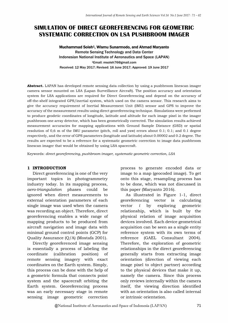
As illustrated in Figure 1-1, direct

georeferencing vector is calculating

vector î by exploring geometric

relationship, which is built by the

physical relation of image acquisition

devices involved. Each device geometrical

acquisition can be seen as a single entity

reference system with its own terms of

reference (GAEL Consultant 2004).

Therefore, the exploration of geometric

relationships in the direct georeferencing

generally starts from extracting image

orientation (direction of viewing each

image pixel to object partner) according

to the physical devices that make it up,

namely the camera. Since this process

only reviews internally within the camera

itself, the viewing direction identified

with an orientation is also called internal

or intrinsic orientation.

mailto:[email protected]

Muchammad Soleh et al.

72 International Journal of Remote Sensing and Earth Sciences Vol.14 No.1 June 2017

Figure 1-1. Geometric point formation of center

of Earth, satellite point on a current time, and

object point or target point forming a vector

relation

Methodologically, formulation of

internal orientation to all cameras were

similar. In order to identify the location of

the image (pixels in the image file) on the

detector cell (pixel detector), which

produced itself, center point of view or

the central perspective identification

inside the lens system was taken as a

point of coordinate system origin. The

coordinate axes defined the right for a

3-D space centered at the origin point,

then calculated the position vector of

each pixel’s detector that represents the

image pixel on the defined camera

coordinate system.

The formulation of internal orientation

(intrinsic vector perspective) was fixed

because of the structure of the camera

was usually a fixed physical construction.

Differences in the formulation of vector

viewing occurs at the technical level, on

how the cameras captured images or

adopted scanning technology being used,

as well as the magnitudes of physical

camera components used. By defining

vector of view internally on physical

devices that produce them, the next step

in the process of exploring the relation of

geometric the direct georeferencing was

to identify the physical relationships

camera with the next physical device

(system). For example, cameras in

non-active mode mounted on the

satellites, and formulate an appropriate

geometric transformation of the camera

reference system to the system, so that it

can be defined as the vector viewpoint

according to the system (satellite).

Furthermore, it was done over and over

in the same steps to connect satellite

systems with Earth, so that the end out

of orientation system was obtained in the

Earth reference system (Maryanto,

2016).

To do direct georeferencing, all of

these parameters (internal and external

orientation of the camera system, GPS

navigation vector viewpoint of the camera

system, and the topography of the Earth

surface) must first be known accurately

enough. It was the primary key to

successfully using direct georeferencing.

If these parameters were highly accurate,

the ground control points would not be

not used (GCP) in rectification process

(Müller et al. 2012).

This research aims to develop a

simulation algorithm on direct

georeferencing and performs simulations

using a pseudo-data. It was done by

building relationships on geometric

image-object, assuming the image data

obtained from pushbroom sensors,

which is mounted on LSA

spacecraft—carrier for pushbroom

linescan type. The simulation described

the spatial error value from simulation by

adjusting the IMU parameters value

(pitch, roll and yaw), GPS parameters

(longitude and latitude) and camera

parameters (length focus). The results

were expected to be a reference for

selecting the specification of IMU and

Simulation of Direct Georeferencing for Geometric Systematic…

International Journal of Remote Sensing and Earth Sciences Vol.14 No.1 June 2017 73

GPS requirement considering their

accuracies.

2 SENSOR ORIENTATION OF THE

PUSHBROOM LINESCAN IMAGER

2.1 Pushbroom Sensor in a Spacecraft

In the acquisition geometry context,

pushbroom sensor can be described

simply as a system in the field of focus

lens array detector mounted straight

(linear detector arrays, for example CCD)

as recording image formed by the lens

system. Since the detector is only a cell

array or detector pixels that form a

straight line, then the image is only in the

form of a picture line elements which has

very small width, so that it can be

regarded as one-dimensional image. 2

dimensional (2D) in pushbroom imager is

only formed if the camera is shifted

regularly when the camera takes images

in accordance to the width of each line of

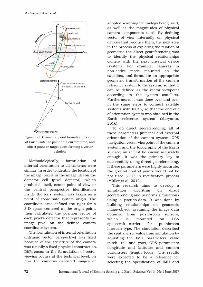
the image as shown in Figure 2-1.

Figure 2-1. Imaging principle with line scanning

technique (pushbroom). 2D image is obtained

through hundreds to thousands of times

shooting with camera panning is the right of the

places in each and every shot.

In remote sensing satellites system,

satellites with pushbroom sensors shoot

hundreds to thousands with set range

times and adapted to flying speed of the

satellite relative to the Earth and with

specified line width size of the image

(spatial resolution) (Maryanto 2016).

2.2 Internal Pushbroom Sensor

Orientation

Internal orientation on pushbroom

imager can be formulated through

mapping (transformation) the location of

the image pixel array detector and the

identification of the physical structure of

the camera as a whole, which is located

inside the detector array. In this case, we

involved the image coordinate system

(ICS), which became input parameters of

the detector coordinate system (DCS).

DCS was also the input parameters to

the camera coordinate system (CCS).

CCS in this case was the data position

(latitude, longitude) and the

attitude/attitude of the camera (roll,

pitch, yaw) or abbreviated LLA (latitude,

longitude, attitude). LLA at CCS

parameters were obtained from the

geo-location using GPS (Global

Positioning System) receiver sensor

devices and IMU (Inertial Measurement

Unit) attitude sensors, which was

mounted on the camera system (Poli

2005). Detail explanations are discussed

in the methods section.

2.3 External Pushbroom Sensor

Orientation

The external orientation of pushbroom

imager can be formulated as relations

established between the camera sensor

and the Earth as a reference, called:

relation between the camera sensor and

the carrier sensor (Spacecraft/Aircraft),

relation between the camera sensor and

the reference system of local orbital. The

local orbital relationships towards the

Earth and the intersection of the viewing

direction of the sensor carrier on the

Earth surface produced the coordinates

of the objects. All parameters of the

relationship mentioned above, will be

taken into account to obtain the

coordinates of the image on Aircraft (LSA)

or Aircraft Coordinate System (ACS).

Moreover, the relationship between ACS

toward the movement of the Earth

(rotation), and then the factor of Earth's

rotation will change ACS into Rotated

Aircraft Coordinate System (RACS) need

to be considered. The last part was RACS

orientation towards the Earth's surface.

To change the RACS orientation into

Earth Coordinate System (ECS) at each

pixel of image data, the intersection of

image coordinates and coordinates on



the Earth's surface need to be calculated

(Poli 2005). Detail explanations are

discussed in method section.

2.4 Coordinate Transformation from

Geocentric to Geodetic Coordinate

To obtain the geocentric coordinates,

we calculated the internal and external

orientation sensor to the Earth. After

getting geocentric coordinates, the final

stage was to transform geocentric

coordinates into geodetic coordinates by

calculating the point of intersection

image pixel’s vector direction with the

Earth’s ellipsoid as a reference for

determining the position vector image

point on the Earth surface. This

transformation process will changed the

position vector to the geographical

coordinates of latitude and longitude

geocentric and subsequently changed the

geocentric geographic coordinates of

latitude and longitude geographic

coordinates to geodetic (Rizaldy and

Firdaus 2012).

There were many ways to perform the

transformation from geocentric to

geodetic coordinates, or vice versa. One

of the popular ways was to involve the

tangential component of the geocentric

latitude of the ellipsoidal Earth

(Jacobsen 2002). In this case, the

process enforced the intersection of

image pixel direction vector with ellipsoid

Earth as a reference for determining the

position vector of each image point on the

Earth's surface. The vector of the Earth's

surface was determined by ellipsoidal

formula corresponding with standard

Earth Flattening parameter WGS-84.

This stage produced ECS in ECEF

coordinates (Jacobsen and Helge 2004).

Finally, after obtaining a vector

pointing intersections of each pixel with

the Earth's surface, it was time to change

back to the vectors ECEF coordinate

system into LLA coordinates (longitude,

latitude, altitude) (Schroth 2004).

However, in this simulations, we assume

that the height (altitude) of each pixel in

the image data was 0 (zero) meter. Detail

explanations are discussed in the

methods section.

3 MATERIALS AND METHODOLOGY

General algorithm which was

commonly used in the process of direct

georeferencing were as follow: data input

position (latitude, longitude) and the

attitude of the camera (roll, pitch, yaw) or

abbreviated as LLA (latitude, longitude,

attitude) obtained from the geo-location

by using pseudo-data derived from the

GPS sensor receiver and IMU sensor

which were mounted on the camera

system. Input parameters of the

pushbroom linescan imager used in this

research were: the number of pixels at

2048, detector’s length at 28.672 mm,

and the camera’s focal length at 35 mm.

This research has built an algorithm

to directly calibrated the image geometric

(direct georeferencing) as shown in

Figure 3-1. In this case, the general

process of direct georeferencing was done

in following stages:

1) Assigning a formula or defining the

internal orientation of the image

pixels on the camera system;

2) Establishing formulas or

relationships, which states the

orientation of the image pixel in the

satellite reference system;

3) Calculating the calendar at the time

an image pixel was obtained;

4) Calculating the position and attitude

of the satellite at the time of taking

the image pixel was done

5) Calculating the direction vector

image pixel on the orbital reference

system;

6) Calculating the direction of vector

image pixel on the earth’s reference

system;

7) Calculating the intersection vector

point of the image pixels direction

with referenced ellipsoid Earth to

determine the position vector image

point on the Earth's surface, namely:

Changing the position vector into

the geographical geodetic latitude



and longitude geocentric

coordinates;

Changing the geocentric geographic

coordinates into geodetic latitude

and longitude geographic

coordinates.

Figure 3-1. General algorithm of direct

georeferencing for linescan pushbroom

imager camera

Direct georeferencing program’s

processing flowchart is shown in Figure

3-1. In general, direct georeferencing

process was a process of projecting each

point sensor (pixel) on the Earth surface

with intersection principle. However, to

use the intersection, the sensor position

and the Earth's surface must be on the

same coordinate system. Then the sensor

operation toward the attitude (roll, pitch,

yaw) was running on ACS system, while

the intersection was running on ECS

system.

3.1 Input Parameters: GPS and IMU

The input parameters in this study

were come from two sensors, i.e. position

interpolation parameters derived from

the GPS and attitude parameters derived

from the IMU. Interpolation of these two

sensors in this study was built with

pseudo-data. The first parameter input

was the LLA position (interpolation GPS

sensor such as latitude, longitude,

altitude) per line, which is known from

GPS receiver. After that the LLA value

was converted into ECEF coordinates

(Earth Centered Earth Fixed). It was a

reference terrestrial conventionally as a

frame of reference with Earth as the

center (geocentric). It went along with the

Earth’s rotation with the origin point at

the center of mass of the Earth. The

positive X direction was the point of

intersection of the equator at longitude

zero. The direction of the earth’s rotation

axis towards the north pole was the

direction of the positive Z-axis, while

multiplying the cross direction of the

positive Z-axis with positive X-axis was

as the Y-axis positive direction according

to the rules of right hand. ECEF

coordinate system has been defined by

the Bureau International de l'Heure (BIH),

and it was equal to the geocentric

reference system U.S. Department of

Defense World Geodetic System 1984 or

known as WGS-84. The purpose of

changing LLA into ECEF was to obtain

the coordinates referring to ECS. The

output will then be used as the origin of

the sensor for each line on linescan.

The second input parameter comes

from an attitude sensor (IMU sensor

interpolation in the form of roll, pitch,

yaw (relative to magnetic north)) derived

from the IMU. Both of GPS and IMU in

this simulation are assumed ideal and we

can give some errors to test the

accuration. Other input parameters was

derived from pushbroom linescan imager

camera sensor, which was used with the

number of pixels in 2048, 28.672 mm

length detector. The camera lens focal

length was at 35 mm. The third

parameter of this input will be processed

by using the Python programming to

generate output coordinates of longitude

and latitude at each pixel on the detector

linescan pushbroom.

3.2 Coordinate Transformation LLA

into ECS (ECEF)

To transform the LLA coordinate

values into ECEF coordinates, we should

change the GPS input sensor coordinate

system, from LLA into ECS (in

ECEF). The Earth parameter used was

WGS-84, as shown in Figure 3-2.

LLA coordinate transformation into

the equation ECEF was done using this

following formula:

𝑥 = (𝑅𝑁 + ℎ) cos 𝜙 cos 𝜆 (1)

𝑦 = (𝑅𝑁 + ℎ) cos 𝜙 sin 𝜆 (2)

𝑥 = ([1 − 𝑒2]𝑅𝑁 + ℎ) sin 𝜙 (3)



Where: 𝜙 = Latitude, 𝜆 = Longitude and h

= Altitude,

with:

𝑅𝑁 =𝑎

√1−𝑒2𝑠𝑖𝑛2∅ (4)

where: a = Earth Equator Radius, e =

eccentricity (with WGS-84 parameter).

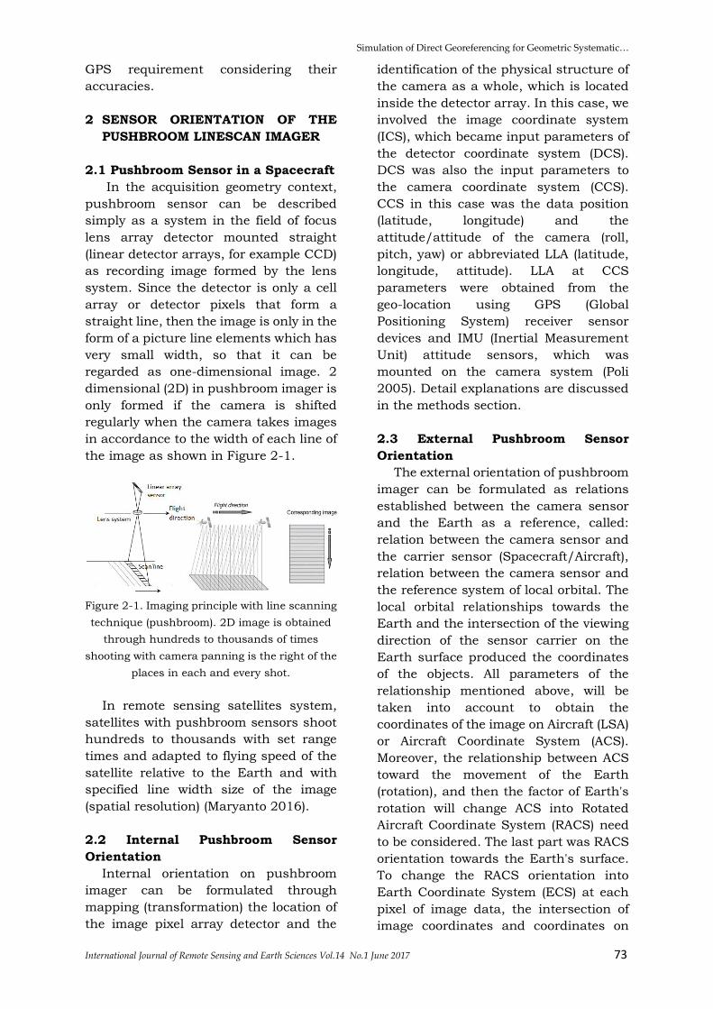
Figure 3-2. Convert parameter calculation

for LLA into ECEF according to ECS

Coordinate output was in Cartesian (x,

y, z) with the center of the Earth

(geocentric) as the center coordinates,

the z axis leads to the zenith geographical

axes of the Earth, the x-axis lead to the

longitude 0°, and the y-axis completes

the z-axis and x according to the rules

hand right as shown in Figure 3-2. The

output will be used as the origin of the

sensor for each line on linescan.

3.3. Coordinate Transformation from

ECS (ECEF) into ACS

After obtaining the ECEF coordinates

which refers to ECS, the ECS was then

applied to calculate the position of the

spacecraft toward the Earth. ECS was

then converted into ACS. In this case, the

Earth coordinates center becomes the

spacecraft coordinates center (sensor).

ACS was a representation to determine

the position of the spacecraft that brings

the sensor to the Earth where the X-axis

leads to true north, the Y-axis east leads

to the east and the Z-axis and leads to

the Earth center geocentric as the right

hand rule. The process of converting ECS

into ACS was done by transforming

matrix as illustrated in Figure 3-3.

Figure 3-3. Calculation of transformation matrix

to implement ECS coordinates into ACS

The coordinate matrix will be used as

the inverse of RACS into ECS. The

transformation of ECS coordinate (ECEF)

into ACS was conducted by the equation:

𝑟𝐸𝐶𝑆 = [

𝑥𝐸𝐶𝑆

𝑦𝐸𝐶𝑆

𝑧𝐸𝐶𝑆

] (5)

𝑒𝑧⃗⃗⃗⃗ �⃗�𝐶𝑆 = −𝑟𝐸𝐶𝑆

|𝑟𝐸𝐶𝑆| (6)

𝑒𝑦⃗⃗⃗⃗ �⃗�𝐶𝑆 = −𝑒𝑧⃗⃗⃗⃗⃗𝐴𝐶𝑆×𝑧0⃗⃗⃗⃗⃗

|𝑒𝑧⃗⃗⃗⃗⃗𝐴𝐶𝑆×𝑧0⃗⃗⃗⃗⃗| with 𝑧0⃗⃗ ⃗⃗ =[

001

] (7)

𝑒𝑥⃗⃗⃗⃗⃗𝐴𝐶𝑆 = −𝑒𝑦⃗⃗⃗⃗⃗⃗ 𝐴𝐶𝑆×𝑒𝑧⃗⃗⃗⃗⃗𝐴𝐶𝑆

|𝑒𝑦⃗⃗⃗⃗⃗⃗ 𝐴𝐶𝑆×𝑒𝑧⃗⃗⃗⃗⃗𝐴𝐶𝑆| (8)

𝑀𝐸𝐶𝑆→𝐴𝐶𝑆 (𝑟𝑜𝑤)= [

𝑒𝑥⃗⃗⃗⃗⃗𝐴𝐶𝑆

𝑒𝑦⃗⃗⃗⃗ �⃗�𝐶𝑆

𝑒𝑧⃗⃗⃗⃗ �⃗�𝐶𝑆

] (9)

3.4. Coordinate Transformation from

ACS into RACS

Rotation operation on spacecraft

coordinate system was based on the

attitude sensor’s input (IMU). The

principle used was that the positive angle

roll (θ) which means rotation angle on the

X-axis opposite clockwise, the positive

pitch angle (ρ) was the rotation angle on

the Y-axis counterclockwise, and the

positive yaw angle (γ) was the rotation

angle on the Z-axis counterclockwise.

With the initial position Pointing pixel in

the Z axis (0,0,1) as shown in Figure 3-4.



Figure 3-4. Operation rotate the camera sensor

pushbroom linescan referring to RACS

ACS coordinates rotation operation

RACS was done with the equation:

𝑀𝑟𝑜𝑡_𝑟𝑜𝑙𝑙 = [1 0 00 cos �́� − sin �́�0 sin �́� cos 𝜃

] (10)

𝑀𝑟𝑜𝑡_𝑝𝑖𝑡𝑐ℎ = [

cos 𝜌 0 sin 𝜌0 1 0

− sin 𝜌 0 cos 𝜌] (11)

𝑀𝑟𝑜𝑡_𝑦𝑎𝑤 = [cos 𝛾 − sin 𝛾 0sin 𝛾 cos 𝛾 0

0 0 1] (12)

As shown in Figure 6 above, after

acquiring RACS, we then performed

rotation (pitch (ρ), roll (θ), yaw (γ)) at

pushbroom linescan camera sensor. In

this case, the scan pixels in one row

occurs at the same time and placed on

the X-axis rotation (roll) perpendicular to

the direction of motion of the aircraft. If

the roll angle was positive, the aircraft

turned to the right and if pitch angle was

positive, the pitch angle of the aircraft up

to the top.

Operation rotation of aircraft

coordinate system was based on the

input from the attitude sensor (IMU). The

principle used was the positive angle of

roll (θ) which was rotation angle on the X-

axis counterclockwise, the positive pitch

angle (ρ) was the rotation angle on the

Y-axis counter-clockwise, and the

positive angle of yaw (γ) was the rotation

angle on the Z-axis counterclockwise. In

this case, the assumption that each pixel

on one line applying roll rotational

operation as shown in Figure 3-5.

Figure 3-5. Pushbroom linescan camera

sensor orientation toward the Earth

referring to RACS

The roll angle per-pixel in one line was

formulated as follow:

�́� = 𝜃 + 𝜓(𝑖) (13)

𝜓(𝑖) = tan−1 ((

𝑖

2−0.5)

(𝑛

2)

.𝑙

𝑓) (14)

Then, the transformation matrix in each

pixel was:

𝑀𝑅𝐴𝐶𝑆 = 𝑀𝑟𝑜𝑡_𝑦𝑎𝑤 . 𝑀𝑟𝑜𝑡_𝑝𝑖𝑡𝑐ℎ. 𝑀𝑟𝑜𝑡_𝑟𝑜𝑙𝑙 . [001

] (15)

3.5. RACS Inverse Coordinate Back

into ECS (ECEF)

After the coordinate values of each

pixel on the sensor was obtained, the

next stage was to inverse RACS

coordinate values into the ECS or ECEF

coordinate. This was done to reverse the

transformation value coordinates on the

sensor to the Earth by vector pointing

from each pixel on the sensor and finding

the correlation of its value toward the

coordinates on the Earth in ECEF

reference frame as shown in Figure 3-6.

The operation was to change RACS

into ECS for each pixel in one line using

the following equations:

𝑃𝐸𝐶𝑆 = (𝑀𝐸𝐶𝑆→𝐴𝐶𝑆)−1. 𝑀𝑅𝐴𝐶𝑆 (16)

�⃗⃗� = 𝑀𝑅𝐴𝐶𝑆→𝐸𝐶𝑆. 𝑀𝑟𝑜𝑡 (17)



Figure 3-6. Sensor coordinate inverse value on

RACS into ECS coordinate system (ECEF)

3.6 Pixel Pointing Intersection

towards the Earth Surface

Referring to the shape of the Earth's

surface, there should be a vector pointing

intersection in each pixel on the sensor to

the ellipsoid Earth surface shaped with

referenced to the Earth‘s ellipsoidal

equation to produce the intersection

value that was closest to the Earth

ellipsoidal field as shown in Figure 3-7.

Figure 3-7. Vector pointing intersection

per-pixel on sensor toward the ellipsoid

Earth surface

The intersection process assumed that

the extension of the pointing vector of

each pixel (𝑃𝐸𝐶𝑆) will intersect

(intersection) with the Earth's surface,

which was defined by the equation:

[𝑥𝑦𝑧

] = [

𝑥𝐸𝐶𝑆

𝑦𝐸𝐶𝑆

𝑧𝐸𝐶𝑆

] + 𝑡. [

𝑥𝑝

𝑦𝑝

𝑧𝑝

] (18)

or

�⃗⃗� = 𝑟𝐸𝐶𝑆⃗⃗ ⃗⃗ ⃗⃗ ⃗⃗ + 𝑡. �⃗⃗� (19)

t is the sought extension of a vector

pointing pixel scale (𝑥𝑝, 𝑦𝑝, 𝑧𝑝). While the

Earth's surface vector (𝑥𝐸𝐶𝑆, 𝑦𝐸𝐶𝑆, 𝑧𝐸𝐶𝑆 ) is

determined by the ellipsoidal formula

according to the WGS84 Earth Flattening

parameters as follows:

𝑥2+ 𝑦2

𝑎2 +𝑧2

𝑏2 = 1 (20)

Where: a = 6378137 m, b =

6356752.3142 m (WGS-84 parameter)

Therefore, to get t value, the two formulas

above became:

(𝑏2𝑥𝑣2 + 𝑏2𝑦𝑣

2 + 𝑎2𝑧𝑣2)𝑡2 + (𝑏2𝑥𝐸𝐶𝑆𝑥𝑣 +

𝑏2𝑦𝐸𝐶𝑆𝑦𝑣+𝑎2𝑧𝐸𝐶𝑆𝑧𝑣)2𝑡 + 𝑏2𝑥𝐸𝐶𝑆2 +

𝑏2𝑦𝐸𝐶𝑆2 +𝑎2𝑧𝐸𝐶𝑆

2 − 𝑎2𝑏2 = 0 (21)

3.7 Conversion of ECS (ECEF) Pixel

Value into Latitude and Longitude

The final stage of direct georeferencing

was to get the coordinates of geocoded

Earth, which was in accordance with the

rules of mapping. To obtain the

coordinates of the geocoded Earth, the

next stage was to change the result of the

intersection vector in ECEF coordinates

obtained into latitude and longitude

coordinates for each pixel in the image.

In this case, it was assumed that the

height of the intersection is 0 (zero)

meters above the surface of the

ellipsoidal Earth. So with tangential

mathematical equation, the latitude and

longitude coordinates for each pixel in

the image as shown in Figure 3-8 can be

obtained.

Figure 3-8. Changing the vector intersection

(ECEF) into Latitude and Longitude coordinates

for each pixel



To change back the ECEF coordinate

systems into the Latitude and Longitude,

the following formula was used:

Longitude:

�̌�(𝑖) = tan2−1(𝑦𝑖, 𝑥𝑖) (22)

and,

Latitude:

�̌�(𝑖) = tan−1 (𝑧𝑖

(1−𝑒2)√𝑥𝑖2+𝑦𝑖

2) (23)

3.8 Horizontal Accuracy Standards for

Geospatial Data

Based on ASPRS 1990’s map accuracy

class, we can compare the simulation’s

accuracy with the ASPRS legacy

standard referred to Ground sample

distance (GSD) that will be generated.

GSD explained the linear dimension of

a sample pixel’s footprint on the ground.

GSD was used when referring to the

collection GSD of the raw image,

assuming near-vertical imagery. The

actual GSD of each pixel was not uniform

throughout the raw image and varies

significantly with terrain height and

other factors. GSD was assumed to be

the value computed using the calibrated

camera focal length and camera height

above average horizontal terrain (ASPRS

2015).

To achieve the horizontal accuracy of

imagery produced, we calculated the

Root-Mean-Square Error (RMSE).

Horizontal accuracy means the

horizontal (radial) component of the

positional accuracy of a data set with

respect to a horizontal datum, at a

specified confidence level. And RMSE

was the square root of the average of the

set of squared differences between data

set coordinate values and coordinate

values from an independent source of

higher accuracy for identical points.

The accuracy test was referring to

coordinate difference (x,y,z) between

image coordinate and the true position

coordinate on the Earth surface. This test

was done to obtained 90% Circular Error

(CE 90) trust level. RMSE calculated with

the following formula:

𝑅𝑀𝑆𝐸𝑟 = √𝑅𝑀𝑆𝐸𝑥2 + 𝑅𝑀𝑆𝐸𝑦

2 (24)

Where,

RMSEx = Root-Mean-Square Error of

point x

RMSEy = Root-Mean-Square Error of

point y

Then, the value of CE 90 calculate as

follows:

𝐶𝐸90 = 1,5175 × 𝑅𝑀𝑆𝐸𝑟

4 RESULTS AND DISCUSSION

4.1 Simulation Results

Direct georeferencing simulation used

Python programming language version

2.7 by inserting a sensor input

parameters that will be simulated—the

number of linescan pixels, the focal

length of the lens (focal length), image

length and sensor line length. In this

case, the default value for the pixel

linescan was 2048, the focal length of the

lens (focal length) was 35 mm, the image

length was 512, sensor line length was

28 672 mm. Based on WGS-84

parameters the value of the equatorial

radius (a) was 6,378,137 km, the Earth's

polar radius (b) was 6356752.3142 km

and eccentricity (e2) was

0.00669437999014.

Direct georeferencing simulations

performed on several control parameters

or variables that can affect the results of

the calculation of direct georeferencing in

pushbroom linescan imager imaging

system on a LSA spacecraft. Those

parameters were derived from the GPS

receiver (latitude and longitude), IMU

(roll, pitch, yaw), linescan camera (focal

length and the length detector) and LSA

height/altitude. In this case the values

were set as follows:

1. Camera parameters (the number of

pixels in 2048, the length 28.672 mm

detectors, the focal length of a 35 mm

camera).

2. Position (Longitude 106, -6 latitude,

altitude 1500 m)

From the simulation results with 6

(six) control parameters or variables



mentioned earlier, we obtained the

following results:

a) The attitude (pitch 0, yaw 0),

parameter variables: roll

b) The attitude (roll 0, yaw 0), parameter

variables: pitch

c) The attitude (pitch 0, roll 0), variable

parameters: yaw

d) The attitude (pitch 0, yaw 0, roll 0),

parameter variables: longitude

e) The attitude (pitch 0, yaw 0, roll 0),

parameter variables: latitude

f) The attitude (pitch 0, yaw 0, roll 0),

parameter variables: the focal length

of the camera

The results of the simulation with six

control parameters and variable (ranging

from a to f) are shown in Table 4-1. We

obtained the difference error values for

each simulation.

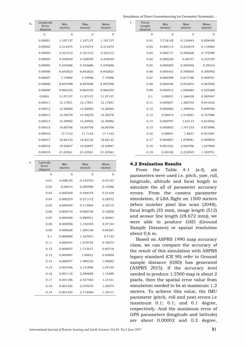
Table 4-1 Deviation measurement results using the 6 control parameters and variables (error is expressed in degrees, while the values of min, max and mean are the distance deviation in meters)

a. Pitch Error

(degree)

Min

(meter)

Max

(meter)

Mean

(meter)

0 0 0 0

0.1 1.745334 1.745357 1.745342

0.2 3.490683 3.49073 3.490699

0.3 5.236057 5.236131 5.236082

0.4 6.981468 6.98157 6.981502

0.5 8.726925 8.727058 8.72697

0.6 10.47244 10.47261 10.4725

0.7 12.21802 12.21823 12.21809

0.8 13.96368 13.96394 13.96377

0.9 15.70944 15.70974 15.70954

1 17.45529 17.45565 17.45541

1.1 19.20125 19.20167 19.20139

1.2 20.94733 20.94782 20.9475

1.3 22.69354 22.69412 22.69374

1.4 24.4399 24.44057 24.44012

1.5 26.18641 26.18717 26.18667

1.6 27.93309 27.93396 27.93338

1.7 29.67994 29.68093 29.68027

1.8 31.42697 31.42809 31.42735

1.9 33.1742 33.17547 33.17462

b. Roll Error

(degree)

Min (meter)

Max (meter)

Mean (meter)

0 0 0 0

0.1 1.745334 1.745357 1.745342

0.2 3.490683 3.49073 3.490699

0.3 5.236057 5.236131 5.236082

0.4 6.981468 6.98157 6.981502

0.5 8.726925 8.727058 8.72697

0.6 10.47244 10.47261 10.4725

0.7 12.21802 12.21823 12.21809

0.8 13.96368 13.96394 13.96377

0.9 15.70944 15.70974 15.70954

1 17.45529 17.45565 17.45541

1.1 19.20125 19.20167 19.20139

1.2 20.94733 20.94782 20.9475

1.3 22.69354 22.69412 22.69374

1.4 24.4399 24.44057 24.44012

1.5 26.18641 26.18717 26.18667

1.6 27.93309 27.93396 27.93338

1.7 29.67994 29.68093 29.68027

1.8 31.42697 31.42809 31.42735

1.9 33.1742 33.17547 33.17462

c. Yaw Error

(degree)

Min (meter)

Max (meter)

Mean (meter)

0 0 0 0

0.1 0.000349 0.714548 0.357446

0.2 0.000698 1.429095 0.714892

0.3 0.001047 2.143642 1.072337

0.4 0.001396 2.858187 1.429781

0.5 0.001745 3.572731 1.787224

0.6 0.002094 4.287272 2.144666

0.7 0.002443 5.001811 2.502106

0.8 0.002793 5.716345 2.859544

0.9 0.003142 6.430876 3.216981

1 0.003491 7.145403 3.574414

1.1 0.00384 7.859924 3.931845

1.2 0.004189 8.57444 4.289273

1.3 0.004538 9.288949 4.646698

1.4 0.004887 10.00345 5.004119

1.5 0.005236 10.71795 5.361536

1.6 0.005585 11.43243 5.71895

1.7 0.005934 12.14691 6.076358

1.8 0.006283 12.86138 6.433763

1.9 0.006632 13.57585 6.791162



d. Longitude Error

(degree)

Min (meter)

Max (meter)

Mean (meter)

0 0 0 0

0.00001 1.107137 1.107137 1.107137

0.00002 2.214274 2.214274 2.214274

0.00003 3.321412 3.321412 3.321412

0.00004 4.428549 4.428549 4.428549

0.00005 5.535686 5.535686 5.535686

0.00006 6.642823 6.642823 6.642823

0.00007 7.74996 7.74996 7.74996

0.00008 8.857098 8.857098 8.857098

0.00009 9.964235 9.964235 9.964235

0.0001 11.07137 11.07137 11.07137

0.00011 12.17851 12.17851 12.17851

0.00012 13.28565 13.28565 13.28565

0.00013 14.39278 14.39278 14.39278

0.00014 15.49992 15.49992 15.49992

0.00015 16.60706 16.60706 16.60706

0.00016 17.7142 17.7142 17.7142

0.00017 18.82133 18.82133 18.82133

0.00018 19.92847 19.92847 19.92847

0.00019 21.03561 21.03561 21.03561

e. Latitude

Error (degree)

Min

(meter)

Max

(meter)

Mean

(meter)

0 0 0 0

0.01 6.98E-05 0.142793 0.07143

0.02 0.00014 0.285586 0.14286

0.03 0.000209 0.428379 0.21429

0.04 0.000279 0.571172 0.28572

0.05 0.000349 0.713965 0.35715

0.06 0.000419 0.856758 0.42858

0.07 0.000488 0.999551 0.50001

0.08 0.000558 1.142345 0.57144

0.09 0.000628 1.285138 0.64287

0.1 0.000698 1.427931 0.7143

0.11 0.000767 1.570724 0.78573

0.12 0.000837 1.713517 0.85716

0.13 0.000907 1.85631 0.92859

0.14 0.000977 1.999103 1.00002

0.15 0.001046 2.141896 1.07145

0.16 0.001116 2.284689 1.14288

0.17 0.001186 2.427482 1.21431

0.18 0.001256 2.570276 1.28574

0.19 0.001325 2.713069 1.35717

f. Focus Length

(degree)

Min (meter)

Max (meter)

Mean (meter)

0 0 0 0

0.01 5.71E-05 0.116943 0.058499

0.02 0.000114 0.233819 0.116964

0.03 0.000171 0.350628 0.175396

0.04 0.000228 0.46737 0.233795

0.05 0.000285 0.584046 0.29216

0.06 0.000342 0.700655 0.350492

0.07 0.000399 0.817198 0.408791

0.08 0.000456 0.933674 0.467056

0.09 0.000513 1.050084 0.525288

0.1 0.00057 1.166428 0.583487

0.11 0.000627 1.282705 0.641653

0.12 0.000683 1.398916 0.699786

0.13 0.00074 1.515061 0.757886

0.14 0.000797 1.63114 0.815952

0.15 0.000853 1.747153 0.873986

0.16 0.00091 1.8631 0.931987

0.17 0.000967 1.978981 0.989954

0.18 0.001023 2.094796 1.047889

0.19 0.00108 2.210545 1.105791

4.2 Evaluation Results

From the Table 4-1 (a-f), six

parameters were used i.e. pitch, yaw, roll,

longitude, altitude and focal length to

simulate the all of parameter accuracy

errors. From the camera parameter

simulation, if LSA flight on 1500 meters

(when number pixel line scan (2048),

focal length (35 mm), image length (512)

and sensor line length (28.672 mm)), we

were able to produce GSD (Ground

Sample Distance) or spatial resolution

about 0,6 m.

Based on ASPRS 1990 map accuracy

class, we can compare the accuracy of

the result of this simulation with ASPRS

legacy standard (CE 90) refer to Ground

sample distance (GSD) has generated (ASPRS 2015). If the accuracy level

needed to produce 1:2500 map is about 2

pixels, then the spatial error value from

simulation needed to be at maximum 1.2

meters. To achieve this value, the IMU

parameter (pitch, roll and yaw) errors i.e

maximum 0.1; 0.1; and 0.1 degree,

respectively. And the maximum error of

GPS parameters (longitude and latitude)

are about 0.00002 and 0.2 degree,



respectively. And then the maximum

error of camera focus is about 0.2 degree.

Based on these 6 simulations with

variable parameters, we can say that in

order to design a pushbroom linescan

imager system in LSA spacecraft, it is

very important to note the selection of

IMU sensor and GPS to improve the

accuracy of the measurement results

using direct georeferencing technique.

Error value of roll, pitch, yaw sensor from

IMU attitude and longitude position, as

well as latitude from GPS, need to be

carefully selected in order to improve the

accuracy of the measurement results

with the direct georeferencing technique.

5 CONCLUSION

The accuracy requirement of camera

sensor, GPS and IMU parameters are

very important parameters to design a

pushbroom linescan imager system in

LSA spacecraft to improve the accuracy

of the measurement results by using the

direct georeferencing technique. The

simulation results showed that the

accuracy requirements of the camera

sensors on the LSA which are derived

using direct georeferencing method can

be determined for mapping applications

by selecting the required Inertial or GPS

equipments. For example, if GSD is 0.6 m,

the specification of Inertial or GPS

equipments must have the maximum

error of the IMU parameter (pitch, roll

and yaw) is 0.1; 0.1; and 0.1 degrees and

the maximum error of the GPS parameter

(longitude and latitude) is 0.00002 and

0.2 degree. This process needs to be

conducted in the early stage in order to

produce corrected and coded systematic

geometrically images to a map or

geocoded image.

ACKNOWLEDGEMENTS

The author would like to thank

Remote Sensing Technology and Data

Center LAPAN in providing data and

software for simulation and as well as

the Journal Editorial Team and

anonymous reviewers in reviewing and

publishing this paper.

REFERENCES

ASPRS, (2015), ASPRS Positional Accuracy

Standards for Digital Geospatial Data,

Photogrammetric Engineering & Remote

Sensing 81(3): A1–A26.

GAEL Consultant, (2004), SPOT Satellite

Geometry Handbook Edition 1, issue 1

revision 4 France, January 2004.

Jacobsen K., (2002), Calibration aspects in

direct georeferencing of frame imagery.

International Archives of Photogrammetry

Remote Sensing and Spatial Information

Sciences, 34(1): 82-88.

Jacobsen K., Helge W., (2004), Dependencies

and Problems of Direct Sensor Orientation.

Proceedings of ISPRS Congress Commission

III.

Maryanto A, Widijatmiko N, Sunarmodo W,

Soleh M, Arief R., (2016), Development of

Pushbroom Airborne Camera System Using

Multispectrum Line Scan Industrial Camera.

International Journal of Remote Sensing and

Earth Sciences (IJReSES), 13(1): 27-38.

Mostafa MMR, Hutton J, Lithopous E., (2001),

Aircraft Direct Georeferencing of Frame

Imagery: An Error Budget, The 3rd

International Symposium on Mobile Mapping

Technology, Cairo, Egypt, January 3-5, 2001

Müller R, Lehner M, Müller R, Reinartz P.,

Schroeder M, Vollmer B., (2012), A Program

for Direct Georeferencing Of Aircraft and

Spacecraft Line Scanner Images, DLR

(German Aerospace Center) Wessling,

Germany. Pecora 15/Land Satellite

Information IV/ISPRS Commission I/FI EO S

2002 Conference Proceedings, Volume

XXXIV Part 1, Denver, USA, 2002.

Poli D., (2005), Modelling of Spacecraft Linear

Array Sensors, Dissertation, Swiss Federal

Institute of Technology, Zurich.

Rizaldy A, Firdaus W., (2012), Direct

Georeferencing: A New Standard In

Photogrammetry For High Accuracy

Mapping, International Archives of the

Photogrammetry, Remote Sensing and

Spatial Information Sciences, 2012.

Schroth R., (2004), Direct Geo-Referencing in

Practical Applications. Proceedings of ISPRS

WG1/5 Workshop about Theory, Technology

and Realities of Inertial/GPS Sensor

Orientation, Castelldefels.

SIMULATION OF DIRECT GEOREFERENCING FOR...

Documents

Transcript of SIMULATION OF DIRECT GEOREFERENCING FOR...