lable at ScienceDirect

Environmental Modelling & Software 26 (2011) 1112e1122

Contents lists avai

Environmental Modelling & Software

journal homepage: www.elsevier .com/locate/envsoft

Simulation and sensitivity analysis of carbon storage and fluxes in the New JerseyPinelands

Zewei Miao a, Richard G. Lathrop Jr. a,*, Ming Xu a, Inga P. La Puma a, Kenneth L. Clark b, John Homb,Nicholas Skowronski b, Steve Van Tuyl b

aGrant F. Walton Center for Remote Sensing & Spatial Analysis, Rutgers University, 14 College Farm Road, New Brunswick, NJ 08901-8551, USAb Silas Little Experimental Forest, USDA Forest Services, 501 Four Mile Road, New Lisbon, NJ 08064, USA

a r t i c l e i n f o

Article history:Received 8 December 2010Received in revised form9 March 2011Accepted 14 March 2011Available online 19 April 2011

Keywords:Carbon dynamicsFire effectsEddy covariance towerWxBGC modelNEEGEPThe extended Fourier amplitude sensitivitytest approach (EFAST)

* Corresponding author. Tel.: þ1 732 932 1580; faxE-mail address: lathrop@crssa.rutgers.edu (R.G. La

1364-8152/$ e see front matter � 2011 Elsevier Ltd.doi:10.1016/j.envsoft.2011.03.004

a b s t r a c t

A major challenge in modeling the carbon dynamics of vegetation communities is the proper parame-terization and calibration of eco-physiological variables that are critical determinants of the ecosystemprocess-based model behavior. In this study, we improved and calibrated a biochemical process-basedWxBGC model by using in situ AmeriFlux eddy covariance tower observations. We simulated carbondynamics of fire-dominated forests at tower sites and upscaled the tower site-based simulations toregional scale for the New Jersey Pinelands using LANDSAT-ETM land cover and DAYMET climate data.The Extended Fourier Amplitude Sensitivity Test approach was used to assess the higher-order sensitivityof model to critical eco-physiological parameters. The model predictions of CO2 net ecosystem exchange(NEE) and gross ecosystem production (GEP) were in agreement with the eddy covariance measurementsat the three tower sites in 2005. However, the model showed poor fit in 2006, grossly overestimatingNEE and the ratio of ecosystem respiration to GEP because the model did not reflect the carbon losscaused by severe defoliation related to an outbreak of gypsy moths in that year. The model simulationsindicated that wildfire reduced annual NEE in pine/scrub oak forest, while prescribed burning in oak/pine and pine/oak stands led to temporary increase in NEE for a period 1e2 years post burning. Theuncertainty and sensitivity of the model carbon simulations were mainly attributable to the 2nd- andhigher-order interactions between carbon allocation parameters, specific leaf area and fire mortalityintensity.

� 2011 Elsevier Ltd. All rights reserved.

1. Introduction

Terrestrial ecosystems can serve as either a net carbon sink ora net source, and play an important role in determining carbonstorage and fluxes at regional and global levels (Aber and Driscoll,1997; Law et al., 2001; Walther et al., 2002; Sitch et al., 2003;Wang et al., 2010). In the past decade, the rate of sequestration byNorth American forests has been estimated at 0.23 petagrams ofcarbon per year (Goward et al., 2008). This offsets about 13% of thefossil fuel emissions from the continent. However, the uncertaintyabout the estimate of forest carbon flux is as high as nearly 50%(Goward et al., 2008). Part of this uncertainty in quantifying carbonflux is due to carbon dynamics of landscape or regional forestecosystems in response to natural and anthropogenic disturbances(Lane et al., 2010; Wang et al., 2010).

: þ1 732 932 2587.throp).

All rights reserved.

In recent years, great strides have been made through theintegration of spatially-explicit ecosystem models, remote sensingderived land cover, eddy covariance measurements and environ-mental variables to quantify carbon cycling dynamics acrossmultiple spatial and temporal scales (Keane et al., 2002; Rollinset al., 2006; Updegraff et al., 2010). As conventional forest inven-tory techniques and eddy covariance measurements are usefulbenchmarks to determine carbon sequestration for a specificvegetation types in certain landscape settings, ecosystem processmodels provide an important means of estimating the spatial andtemporal details of changes in carbon storage and fluxes (Whiteet al., 2000; Law et al., 2001; Thornton et al., 2002; Pan et al.,2006; Updegraff et al., 2010). Previous literature suggested thatspatially explicit ecosystem models should not only capture themost critical interactions between environmental drivers andecosystem processes, but also accurately convey the impact ofnatural and human disturbances on the processes of CO2 uptake,storage and emission (White et al., 2000; Thornton et al., 2002;Lane et al., 2010; Updegraff et al., 2010). A critical evaluation of

Z. Miao et al. / Environmental Modelling & Software 26 (2011) 1112e1122 1113

a model’s ability to explain the within-site and between-site vari-ability in forest inventory data or flux measurements is essentialbefore broader scale applications of the model can be pursued (Lawet al., 2001; Thornton et al., 2002; Pan et al., 2006). Thus, there isa growing need for coupled observational and modeling strategiesto simulate and map response of carbon storage and cycling tonatural and human disturbances for particular regions of concern.

A key determinant of a model’s utility for specific landscapes orregions is the proper calibration of the model’s driving variableswith locally-applicable parameterization and sensitivity of themodel’s input parameters (Aber et al., 1997; White et al., 2000;Gertner, 2003; Matsushita et al., 2004; Miao et al., 2004, 2009;Makler-Pick et al., 2011). To examine the applicability of theBiome-BGC model across a range of conditions, for example,White et al. (2000) collected highly site- and species-specific eco-physiological parameters for major temperate biomes andassessed the factorial sensitivity of NPP (net primary productivity)for five critical parameters. For a given species or biomes, vari-ances of many eco-physiological parameters are high enough tosignificantly influence prediction quality. For instance, the allo-cation ratio of new stem carbon to new leaf carbon of pitch pine(Pinus rigida Mill.) and white oak (Quercus alba L.) ranged from1.28 to 1.99 and from 0.80 to 1.36, respectively (Olsvig, 1980;White et al., 2000). Specific leaf area of the evergreen needleleaf (ENF) biome varied from 2.8 m2 kgC�1 for Pinus resinosa to11.5 m2 kgC�1 for Pinus taeda of the eastern US forests (Scherzerand Hom, 2008). Thus in approaching a finer scale application ofa broadly parameterized ecosystem process model, carefulattention must be paid to examining this uncertainty. Further, thespecific form and coefficients of the biogeochemical modelequations are generally based on empirical laboratory and/or fieldobservations, and thus are not always applicable under allconditions. Accordingly, sensitivity analyses are prerequisites formodel building and application in any setting, be they diagnosticor prognostic (White et al., 2000; Saltelli, 2002; Saltelli et al.,2000; Miao et al., 2004; Miao and Li, 2007, 2010; Saltelli andAnnoni, 2010).

The objective of this study is (i) to improve and calibrate theWxBGC model tool, a coupled Biome-BGC and WxFIRE model, byusing locally-derived eco-physiological parameters and historicalfire records; (ii) to make higher-order sensitivity and uncertaintyanalysis of the model carbon simulations to eco-physiologicalparameters; and (iii) to simulate andmap carbon storage and fluxesof the US New Jersey Pinelands region. In this study, the WxBGCmodel was modified and validated against AmeriFlux (Long-termflux measurement network of the Americas) eddy covariancemeasurements in representative uplands forests that spanned thegradient from oak/pine to pine/oak to even more heavily firedisturbed pine/scrub oak during the years of 2005 and 2006(Clark et al., 2004, 2009). Sensitivity analysis was carried outthrough the Extended Fourier Amplitude Sensitivity Test (EFAST)approach to examine the main effects and higher-order interac-tions between the eco-physiological input parameters and theircontribution to the uncertainty of carbon dynamic predictions. ThevalidatedWxBGCmodel was then applied across a longer time spanto examine model behavior in relation to fire disturbance andacross the broader New Jersey Pinelands region to predict and mapcarbon dynamics and distribution at the regional scale.

2. Materials and methods

2.1. Model description

The WxBGC model was developed by the USDA Forest Service NationalLANDFIRE project (Steinwand and Nelson, 2005; personal communication) togenerate consistent and comprehensive spatially explicit biophysical layers

containing vegetation, litter, soil carbon, water vapor, fire disturbances, etc. ofMulti-Resolution Land Characterization (MRLC) zones, in support of the USnational LANDFIRE prototype and vegetation mapping. The WxBGC model inte-grate the WxFIRE and Biome-BGC models and is able to implement parallelsimulations for large-scale landscape ecosystems at a finer resolution on a Linux(Red Hat 8.0)-based multiple-node cluster. As a widely calibrated model, theBiome-BGC model seeks to mechanistically represent ecosystem cycles of carbon,water, and nutrients through an integrated consideration of biology andgeochemistry (Running and Gower, 1991; White et al., 2000; Thornton et al., 2002).The WxFIRE model is used to map vegetation, fuels, fire regimes and fire conditionclasses in the LANDFIRE project, and computes climate-based biophysical variablesat any landscape scale or resolution using daily weather data, topography and soilparameters, and a diverse set of integrated environmental functions (Keane et al.,2002). Detailed descriptions of the Biome-BGC and WxFIRE models can be foundin Running and Gower (1991), Thornton et al. (2002) and Keane and Holsinger(2005), respectively.

In the current study, we modified the WxBGC model to simulate carbon storageand dynamics of the New Jersey Pinelands. The model improvements are summa-rized as follows:

(i) Combination of random and spatially heterogeneous fire disturbances into themodel. Inherited from the Biome-BGC model, the original WxBGC model setdisturbance intensity (i.e., the whole-plant mortality rate parameters)through plant eco-physiological parameter input files and considered distur-bance as a continuous and spatially homogenous disturbance. In other words,disturbance occurs at every pixel every time step with a constant intensity.The assumption may be true for chronic harvest cutting, herbivory and insectdefoliation within large areas, but may not be applicable to episodic andspatially heterogeneous disturbances such as wildfire and windfall. Based onour review of historical fire occurrence records of the New Jersey Pinelands forthe years between 1924 and 2007, we improved the model to randomlygenerate fire events between March and April for spring prescribed burningby using uniform random distribution and stochastically initiate wildfireevent dates using a Gaussian distribution. In this study, we set April 20 as themean and 40 days as the standard deviation of Gaussian distribution for NewJersey pinelands wildfire disturbance events, respectively. Therefore, ourmodified WxBGC version includes stochastic rather than deterministic firedisturbance. We empirically classified fire intensity (i.e., fire mortality rate)into five levels: no fire, prescribed burning (we assumed prescribed fireburned 30% of dead stem, litter and coarsewoody debris, and 5% of live carbonwhich represents burned shrub and grass), moderate non-replacementwildfire (35% of all carbon to be burned), heavy non-replacement wildfire(50% of all carbon to be burned) and replacement wildfire (>60% of all carbonto be burned) (Little, 1979; Boerner, 1981; Boerner et al., 1988). We set firedisturbance to directly reduce a proportion of the initial values of all plant andfine litter state variables immediately before the disturbance as did Thorntonet al. (2002). The affected proportions of the leaf, fine root, live wood, and finelitter C and N pools are assumed to be lost to the atmosphere.

(ii) Combination of remote sensing land cover data into the model. In order togenerate consistent and comprehensive biophysical layers of carbon andwater dynamics of MRLC zones, the original WxBGC model hypotheticallyassumes a spatially homogeneous land cover (i.e., evergreen needle leaf orgrass) for given landscape or region. We coupled remote sensing-derived landcover mosaics into the model to spatially explicitly simulate comprehensivebiophysical layers of real heterogeneous ecosystem mosaics. Except formeteorological data, the improved version includes 11-layers of geo-referencespatial inputs such as elevation (m), aspect (�), slope (%), hillshade (dimen-sionless), soil depth (m), sand percent, silt percent, clay percent, land covertype, fire time and intensity (percent of tree fire mortality). We set othergeographic or environmental variables (e.g., albedo, N-deposition, etc.) toBiome-BGC default values (White et al., 2000; Thornton et al., 2002).

(iii) Improvements of output functions. The original WxBGC model does not outputmonthly and annual predictions but the 18-yr average predictions of 42variables. We restructured the output functions of the WxBGC model intotimely and spatially explicit variable-oriented output functions, i.e., 42monthly and annual biophysical variables including transpiration, actualevapotranspiration, leaf area index, net ecosystem exchange of CO2, grossprimary productivity (GPP), soil carbon, etc. The internal time step of themodel is still daily. Theoretically, themodel could output daily predictions, butoutput file sizes would be as high as over hundreds gigabytes for the NewJersey Pineland at finer resolution (say less than 100-m resolution), thereforethe daily output function was inactivated.

It is worth noting that the original model classified DEM and DEM derivativesinto several group levels and aggregated some similar neighbor pixels into one mapunit to reduce total pixel numbers and computations due to the large spatial scale ofMRLC zone 60. The improved version is straight up the original pixels of land coverand geo-referenced environmental variables.

Z. Miao et al. / Environmental Modelling & Software 26 (2011) 1112e11221114

2.2. Study area

The study was conducted in the New Jersey Pinelands, which consists ofapproximately 1.1 million acres in southern New Jersey. The New Jersey Pinelandswas the first US National Reserve designated as such and a U.S. Biosphere Reserve ofthe Man and the Biosphere Program. Two relatively distinct floristic complexes arepresent in the Pinelands, a lowland complex (wetland) and an upland complex. Thewetlands are composed principally of white cedar (Chamaecyparis thyoides (L.)B.S.P.), trident red maple (Acer rubrum L.), and black gum (Nyssa sylvatica Marsh.).The uplands comprise approximately 62% of the Pine Barrens, and are dominated bythree major forest communities: black oak/pine forest types, pine/black oak, andpine/scrub oak in the understory (McCormick and Jones, 1973; McCormick, 1979;Forman, 1979; Lathrop and Kaplan, 2004; Skowronski et al., 2007). All stands haveericaceous shrubs in the understory, primarily huckleberry (Gaylussacia baccata(Wangenh.) K. Koch, G. frondosa) and blueberry species (Vaccinium spp.)(Skowronski et al., 2007). In the New Jersey Pinelands, fire and human disturbancesare considered as secondary environmental factors in determining vegetationcommunity composition following soil texture and nutrients. Fire frequency is fairlyhigh (e.g., 5e15 yrs for dwarf pine plains and 15e25 years for pitch pine-scrub oakbarrens) and fire disturbances can apparently affect the current process and futuredirection of carbon flux for some forest community types (Boerner, 1981; Formanand Boerner, 1981; Buchholz and Zampella, 1987; Boerner et al., 1988).

In the Pinelands, in winter, a strong northwesterly flow of cold, dry air massesfrom Canada predominates, and temperatures average 0e2 �C (32e36 �F). Insummer, a southwesterly flow of warm, humid air, around the Bermuda high-pressure area dominates the Pinelands, with temperatures averaging 22e24 �C(72e75 �F). Average annual precipitation throughout the Pinelands is1067e1168 mm. Both precipitation and temperatures are highly variable from yearto year (Havens, 1979).

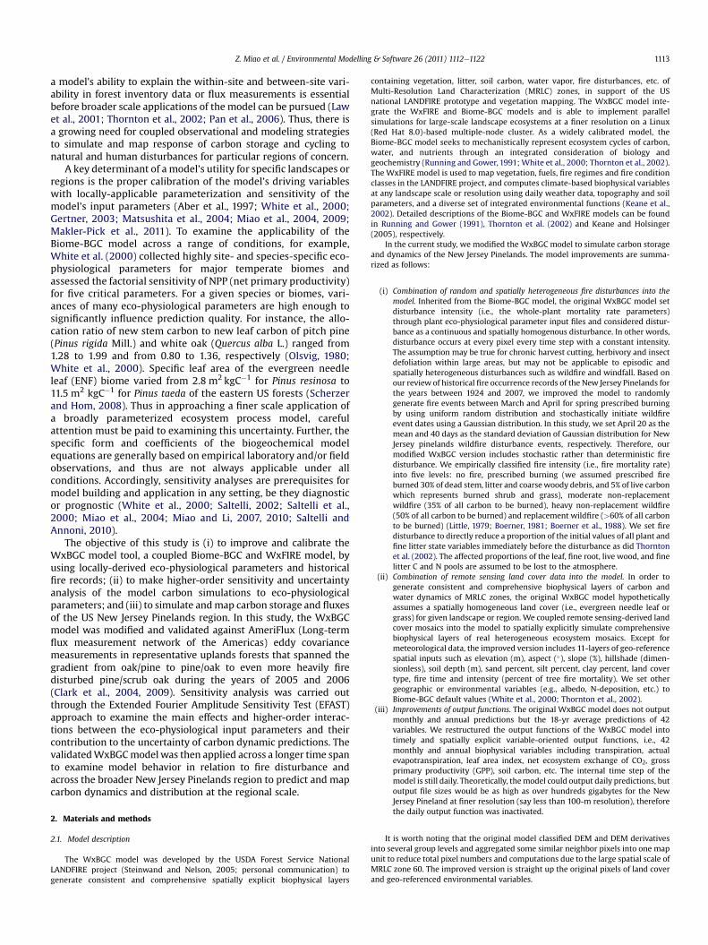
Three upland AmeriFlux eddy tower sites operated by the U.S. Forest Service outof the Silas Little Experimental Forest were used as calibration/validation sites.These sites consisted of a mixed oak and pitch pine stand (oak dominated) (SilasLittle, 39.9161 �N, 74.5986 �W), a mixed pine/oak stand (pine dominated) (Fort Dix,39.9731�N, 74.4341�W), and a pitch pine overstory/scrub Oak dominated understorystand (Cedar Bridge, 39.8302 �N, 74.3403 �W) (Skowronski et al., 2007) (Fig. 1). Theclimate of three sites is cool temperate, with mean monthly temperatures of 0.3 and23.8 �C in January and June (1930e2004), respectively. Mean annual precipitation is1123�182 mm. Soils are derived from the Cohansey and Kirkwood Formations(Lakewood and Sassafras soils), and are coarse-textured, sandy, acidic, and haveextremely low cation exchange capacity and nutrient status (Tedrow, 1986).A wildfire event occurred in 1995 at the Cedar Bridge tower site. Two prescribedburning events occurred in 2002 and 2003 at the Fort Dix tower site. Four prescribedfire events occurred in 1980, 1981, 1982 and 1997 at the Silas Little tower site.

2.3. Remote sensing derived land covers and eco-physiological parameterizations

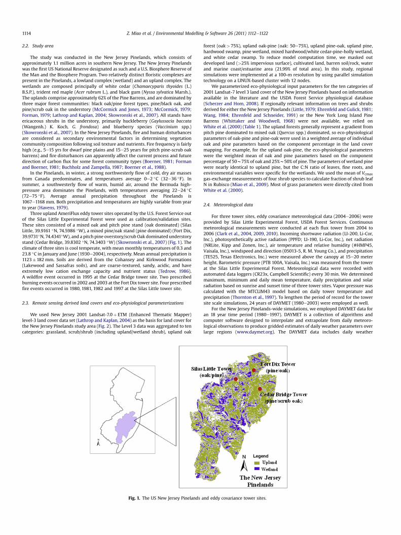
We used New Jersey 2001 Landsat-7.0þ ETM (Enhanced Thematic Mapper)level-3 land cover data set (Lathrop and Kaplan, 2004) as the basis for land cover forthe New Jersey Pinelands study area (Fig. 2). The Level 3 data was aggregated to tencategories: grassland, scrub/shrub (including upland/wetland shrub), upland oak

Fig. 1. The US New Jersey Pinelands

forest (oak> 75%), upland oak-pine (oak: 50e75%), upland pine-oak, upland pine,hardwood swamp, pine wetland, mixed hardwood/white cedar-pine-holly wetland,and white cedar swamp. To reduce model computation time, we masked outdeveloped land (>25% impervious surface), cultivated land, barren soil/rock, waterand marine coast/estuarine area (21.99% of total area). In this study, regionalsimulations were implemented at a 100-m resolution by using parallel simulationtechnology on a LINUX-based cluster with 12 nodes.

We parameterized eco-physiological input parameters for the ten categories of2001 Landsat-7 level 3 land cover of the New Jersey Pinelands based on informationavailable in the literature and the USDA Forest Service physiological database(Scherzer and Hom, 2008). If regionally relevant information on trees and shrubsderived for either the New Jersey Pinelands (Little, 1979; Ehrenfeld and Gulick, 1981;Wang, 1984; Ehrenfeld and Schneider, 1991) or the New York Long Island PineBarrens (Whittaker and Woodwell, 1968) were not available, we relied onWhite et al. (2000) (Table 1). The upland forests generally represent a gradient frompitch pine dominated to mixed oak (Quercus spp.) dominated, so eco-physiologicalparameters of oak-pine and pine-oak were used in a weighted average of individualoak and pine parameters based on the component percentage in the land covermapping. For example, for the upland oak-pine, the eco-physiological parameterswere the weighted mean of oak and pine parameters based on the componentpercentage of 50w75% of oak and 25%w50% of pine. The parameters of wetland pinewere nearly identical to upland pine, but the C:N ratio of leaves, fine roots, andenvironmental variables were specific for the wetlands. We used the mean of Vcmax

gas-exchange measurements of four shrub species to calculate fraction of shrub leafN in Rubisco (Miao et al., 2009). Most of grass parameters were directly cited fromWhite et al. (2000).

2.4. Meteorological data

For three tower sites, eddy covariance meteorological data (2004e2006) wereprovided by Silas Little Experimental Forest, USDA Forest Services. Continuousmeteorological measurements were conducted at each flux tower from 2004 to2006 (Clark et al., 2004, 2009, 2010). Incoming shortwave radiation (LI-200, Li-Cor,Inc.), photosynthetically active radiation (PPFD; LI-190, Li-Cor, Inc.), net radiation(NRLite, Kipp and Zonen, Inc.), air temperature and relative humidity (#HMP45,Vaisala, Inc.), windspeed and direction (05013-5, R. M. Young Co.), and precipitation(TE525, Texas Electronics, Inc.) were measured above the canopy at 15e20 meterheight. Barometric pressure (PTB 100A, Vaisala, Inc.) was measured from the towerat the Silas Little Experimental Forest. Meteorological data were recorded withautomated data loggers (CR23x, Campbell Scientific) every 30 min. We determinedmaximum, minimum and daily mean temperature, daily precipitation and solarradiation based on sunrise and sunset time of three tower sites. Vapor pressure wascalculated with the MTCLIM43 model based on daily tower temperature andprecipitation (Thornton et al., 1997). To lengthen the period of record for the towersite scale simulations, 24 years of DAYMET (1980e2003) were employed as well.

For the New Jersey Pinelands-wide simulations, we employed DAYMET data foran 18 year time period (1980e1997). DAYMET is a collection of algorithms andcomputer software designed to interpolate and extrapolate from daily meteoro-logical observations to produce gridded estimates of daily weather parameters overlarge regions (www.daymet.org). The DAYMET data includes daily weather

and eddy covariance tower sites.

Fig. 2. Input variables and structure of the WxBGC model.

Z. Miao et al. / Environmental Modelling & Software 26 (2011) 1112e1122 1115

parameters such as temperature, precipitation, solar radiation, vapor pressuredeficit and day length, and it was produced on a 1 kilometer grid over the entireconterminous United States for the period of record 1980e1997. The daily obser-vations used to produce the gridded surfaces came from approximately 6000stations in the U.S. National Weather Service Co-op network and the NaturalResources Conservation Service SNOTEL network (automated stations in moun-tainous terrain) (Thornton et al., 1997, 2000; Thornton and Running, 1999).

2.5. Geo-referenced environmental gradients

We used the USDA Natural Resources Conservation Service SSURGO (Soil SurveyGeographic) database (http://soildatamart.nrcs.usda.gov/) to derive soil texture(sand, clay and silt percent) and soil profile depth (soil depth in m) maps for the NJPinelands study area. Elevation (m) and slope (%), aspect (degree) and topographicshade (hillshade) maps were developed from a seamless DEM mosaic of the USGSNational Elevation Database (NED) (http://edc2.usgs.gov/geodata/index.php).

2.6. Eddy covariance towers and NEE measurements

We used closed-path eddy covariance (EC) measurements from the U.S. ForestService’s three eddy tower sites to evaluate the model predictions of net ecosystemexchange (NEE). EC systems were composed of a 3-dimensional sonic anemometer(Windmaster Pro or R3A, Gill Instruments Ltd., Lymington, UK, or RM 80001V, R.M.Young, Inc.) mounted approximately 4 m above the canopy on an antenna tower ateach site, a closed-path infrared gas analyzer (LI-7000, Li-Cor Inc., Lincoln, Nebraska)in an enclosure on the tower, a 5 m long, 0.4 cm ID teflon coated tube and an air pumpsampling 8 lmin�1, and a lap-top PC to collect data (Moncrieff et al., 1997; Clark et al.,2004). The LI-7000s were calibrated every 2e7 days using CO2 tanks that weretraceable to primary standards. Net CO2 exchange was then calculated at half-hourintervals using EdiRe software. The flux associated with the change in storage of CO2

in the air column beneath the inlet was estimated using top of tower and 2-m heightmeasurements or a profile systemwith inlets at 0.2, 2, 5, 10, 15 and 20 m height.

Annual NEE estimates require continuous values of half-hourly CO2 exchange. Toestimate daytime net CO2 exchange (NEEday) for periods when we did not havemeasurements (due to precipitation, low windspeed conditions, instrument failure,etc.), a rectangular hyperbola to the relationship between PPFD and NEEday werefitted (Ruimy et al., 1995; Clark et al., 2004). To estimate nighttime net CO2 exchange(NEEnight), half-hourly net exchange rates were regressed on air or soil temperatureusing an exponential function. We then used modeled data calculated from the

continuous meteorological data for periods when we did not have measured fluxesto estimate daily to annual NEE for each site. Annual ecosystem respiration (Reco)was calculated for each site using continuous half-hourly air or soil temperature.Annual NEE and Reco were summed to estimate gross ecosystem productivity (GEP)(Reichstein et al., 2005; Clark et al., 2009) (Table 2). GPP and GEP are often inter-changeable in the field of ecological modeling, but GEP contains a photorespiratorycomponent that GPP does not (Law et al., 2001; Clark et al., 2004, 2009; Reichsteinet al., 2005).

2.7. Sensitivity and uncertainty analysis

We employed the EFAST approach to analyze the sensitivity of the carbonstorage and flux predictions to 11 crucial eco-physiological input parameters. Asa procedure widely used for uncertainty and sensitivity analysis, the FourierAmplitude Sensitivity Test (FAST) method is more efficient than the Monte Carloapproach and used to estimate the expected value and variance of the output andthe contribution of individual inputs to uncertainty and sensitivity of the outputs(Saltelli, 2002; Frey and Patil, 2002; Saltelli and Annoni, 2010; Yang, 2011). TheEFAST method developed by Saltelli et al. (2000) was used to address higher orderinteractions between the inputs. The EFAST method used a decomposition of theFourier series representation to obtain the fractional contribution of the individualinput variables to the variance of the model predictions (Saltelli and Bolado, 1998;Saltelli et al., 2000; Saltelli, 2002; Frey and Patil, 2002). The total variances of themodel output can be described as:

VðYÞ ¼Xk

i¼1

Vi þXk

i¼1

Xk

j>i

Vij þXk

i¼1

Xk

j>i

Xk

m>j

Vijm þ/þ V12/k

where V(Y) is total unconditional variance of the model output (Y) with k inputvariables, Vi is the first-order conditional variance of the model output (Y) wheninput variable Xi ¼ x*i , i.e., Vi ¼ VðEðYjXi ¼ x*i ÞÞ, x*i is untrue or random value ofXi, Vij is the second-order variance when Xi ¼ x*i and Xj ¼ x*j , i.e., the variance of

the interaction between variables i and j, Vij ¼ VðEðYjXi ¼ x*i ;Xi ¼ x*j ÞÞ � Vi � Vj ,

Vijm and V12/:k are the higher order variance of interaction among multiple (�3)variables i, j, m.k.

The first-order sensitivity index (S) is: Si ¼ Vi=VðYÞ, i.e., the contribution ofindividual parameter to the model performance. Similarly, the second- and higher-order sensitivity index are: Sij ¼ Vij=VðYÞ, Sijm ¼ Vijm=VðYÞ. The total order

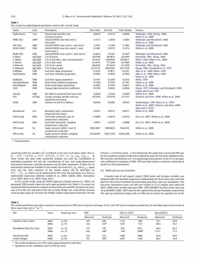
Table 1The crucial eco-physiological parameters used in the current study.

Name Unit Description Silas Little Fort Dix Cedar Bridge Sources

leafturnover 1/yr Annual leaf and fine rootturnover fraction

0.8933 0.5735 0.4609 Whittaker, 1962; Olsvig, 1980;White et al., 2000

NFRC:NLC DIMa (ALLOCATION) new fine root C:new leaf C

1.4173 1.3810 1.3695 Whittaker and Woodwell, 1968;White et al., 2000

NSC:NLC DIM (ALLOCATION) new stem C: new leaf C 1.3501 2.1594 2.1482 Whittaker and Woodwell, 1968NLWC:NWC DIM (ALLOCATION) new live wood C: new

total wood C0.1463 0.1072 0.1674 White et al., 2000

NCRC:NSC DIM (ALLOCATION) new croot C: new stem C 0.3014 0.2187 0.1947 Whittaker and Woodwell, 1968C:Nleaf kgC/kgN C:N of leaves 29.9708 40.0872 42.9395 Ehrenfeld, 1981; Wang, 1984C:Nlitter kgC/kgN C:N of leaf litter, after retranslocation 76.4527 100.0945 103.8611 Melin, 1930; White et al., 2000C:Nfroot kgC/kgN C:N of fine roots 61.9475 57.5269 55.7099 White et al., 2000C:Nlwood kgC/kgN C:N of live wood 88.6978 87.0239 81.7630 Ehrenfeld, 1981; Wang, 1984C:Ndwood kgC/kgN C:N of dead wood 557.6741 608.9501 637.5739 Wang, 1984; Woodwell et al., 1975leaflabile DIM Leaf litter labile proportion 0.3522 0.3871 0.4141 Aber et al., 1990; Melin, 1930leafcellulose DIM Leaf litter cellulose proportion 0.4502 0.3826 0.3505 Aber et al., 1990; Melin, 1930;

White et al., 2000leaflignin DIM Leaf litter lignin proportion 0.1975 0.2303 0.2355 Melin, 1930dwoodcellulose DIM Dead wood cellulose proportion 0.7438 0.7263 0.7185 White et al., 2000dwoodlignin DIM Dead wood lignin proportion 0.2562 0.2738 0.2815 White et al., 2000CLEC DIM Canopy light extinction coefficient 0.5354 0.4024 0.4024 Wood, 1937; Whittaker and Woodwell, 1969;

Collins and Good, 1987LAratio DIM All-sided to projected leaf area ratio 2.0926 2.3563 2.4469 White et al., 2000SLA m2/kgC Canopy average specific leaf area

(projected area basis)20.5545 16.0334 15.3131 Scherzer and Hom, 2008; White et al., 2000

PLNR DIM Fraction of leaf N in Rubisco 0.0520 0.0383 0.0333 Wullschleger, 1993; Reich et al., 1995;White et al., 2000; Scherzer and Hom, 2008;Miao and Li, 2010

Boundcond m/s Boundary layer conductance(projected area basis)

0.0223 0.0575 0.0671 White et al., 2000

LWP:scond MPa Leaf water potential: start ofconductance reduction

�0.2694 �0.4672 �0.5014 Xu et al., 2007; White et al., 2000

LWP:fcond MPa Leaf water potential: completeconductance reduction

�1.8657 �2.1953 �2.4898 Xu et al., 2007; White et al., 2000

VPF:scond Pa Vapor pressure deficit: start ofconductance reduction

1024.3827 809.0625 744.6355 White et al., 2000

VPF:ccond Pa Vapor pressure deficit: completeconductance reduction

3522.8395 3303.1250 3290.1040 White et al., 2000

a Dimensionless.

Z. Miao et al. / Environmental Modelling & Software 26 (2011) 1112e11221116

sensitivity index for variable i (STi ) is defined as the sum of all above index, that is:STi ¼ ðVðYÞ � VðEðYjX�iÞÞÞ=VðYÞ ¼ ðEðVðYjX�iÞÞÞ=VðYÞ ¼ Si þ Sij þ Sijm þ Sijm/k . Inother words, the total order sensitivity includes not only the contribution ofindividual parameter but also the contributions of two- and multi-dimensionalinteractions between a specific parameter and all other parameters. If there are nointeractions among the variables in the model, the terms of Sij , Sijm and Sijm/k equalzero, and the total variances of the model output can be described as:VðYÞ ¼ Pk

i¼1 Vi , which can be addressed by OAT (test one parameter at a time) ormultivariate regression methods (Saltelli et al., 2000; Saltelli, 2002; Matsushitaet al., 2004; Miao et al., 2004; Yang, 2011).

In the current study, using the EFAST approach (SimLab version 2.2, 2003), wegenerated 7000 pseudo values for each input parameter sets (Table 3). In actual, wesimulated 6943 iterations for oak/pine at Silas Little site and 6923 iterations for pine/oak at Fort Dix site and pine/scrub oak at Cedar Bridge site, respectively, becausesome pseudo values do not meet the WxBGC model requirements that the C:N ratio

Table 2The model predictions and eddy covariance measurements of NEE (net ecosystem exchanthree tower sites (gCm�2 yr�1).

Site Years Stand age (yrs) NEE

Observed

Oak/Pine (Silas Little) 2005 ca. 90 1872006 ca. 91 122

Pine/Mixed Oak (Fort Dix) 2005 ca. 74 1372006 ca. 75 �103

Pine/Scrub Oak 2005 ca. 81 222(Cedar Bridge) 2006 ca. 82 161

a The model prediction was GPP, which approximated to GEP here.b Significant at the confidence level of 95% by t-test.

of leaves> C:N of livewood> C:N of deadwood.We undertook a total of 20,789 runsfor the sensitivity analysis of the three vegetation types for the three validation sites.We used the contributions of 11 eco-physiological parameters to the 27-yr averagesand coefficient of variations of NEE, GPP and total carbon to measure sensitivity ofmodel to critical parameters.

2.8. Model spin-up and simulation

A steady state of soil organic matter (SOM) pools and nitrogen variables wasattained under the specified vegetation ecophysiology for three tower sites and eachpixel for New Jersey Pinelands by performing precursor (spin-up) simulations. Theprecursor simulations were run with the respect to 27-yr climate data (observed2004e2006 tower weather data plus 1980e2003 DAYMET) for three tower sites and18-yr DAYMET (1980e1997) data for the regional New Jersey Pinelands, respectively.The spin-up simulations begin with no SOM and are driven by repeated use of the

ge of CO2) and GEP (gross ecosystem production) of naturally-regenerated stands at

GEP (or GPP)a Reco/GEP(%)

Predicted Observed Predicted Observed Predicted

208 1133 866 79.1 76.0218b 1167 913 89.5 76.1

170 876 1012 84.4 83.2249b 784 1090b 113.1 77.2

234 1388 1098 84.0 78.8250b 1403 1160 88.5 78.4

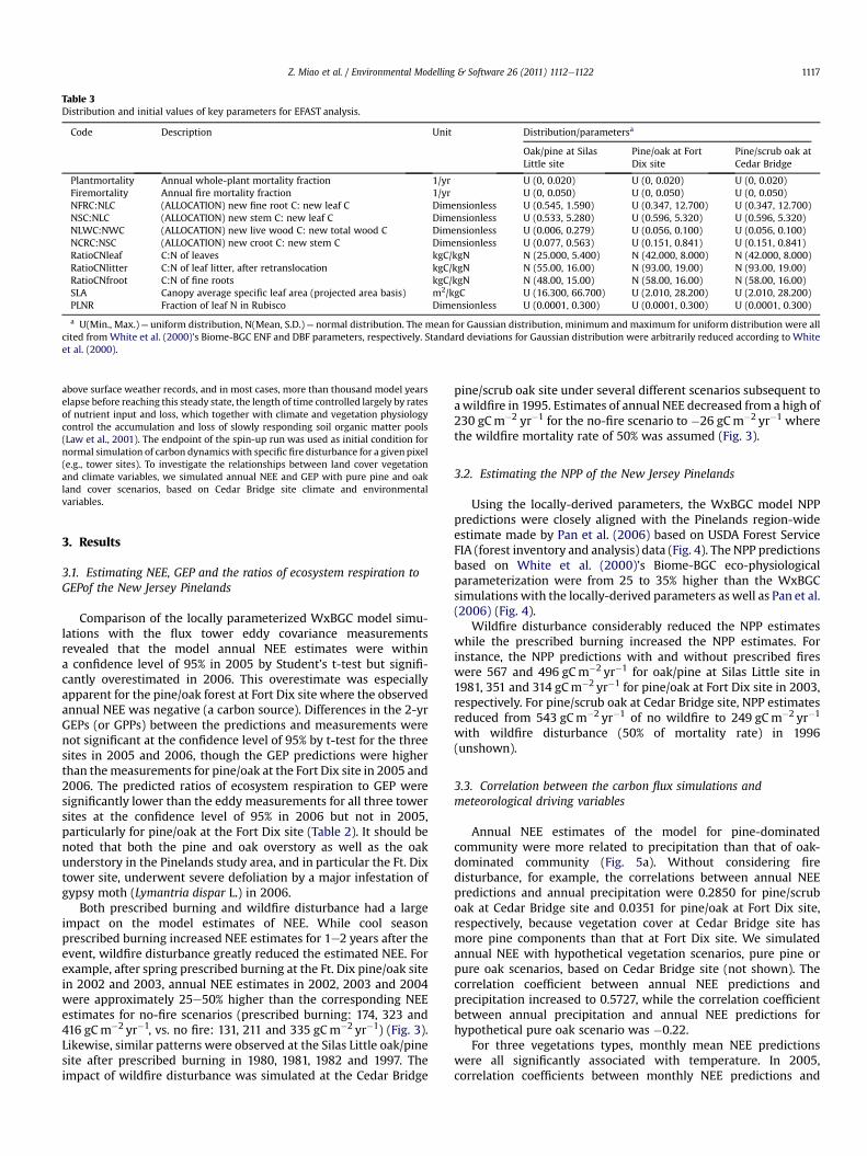
Table 3Distribution and initial values of key parameters for EFAST analysis.

Code Description Unit Distribution/parametersa

Oak/pine at SilasLittle site

Pine/oak at FortDix site

Pine/scrub oak atCedar Bridge

Plantmortality Annual whole-plant mortality fraction 1/yr U (0, 0.020) U (0, 0.020) U (0, 0.020)Firemortality Annual fire mortality fraction 1/yr U (0, 0.050) U (0, 0.050) U (0, 0.050)NFRC:NLC (ALLOCATION) new fine root C: new leaf C Dimensionless U (0.545, 1.590) U (0.347, 12.700) U (0.347, 12.700)NSC:NLC (ALLOCATION) new stem C: new leaf C Dimensionless U (0.533, 5.280) U (0.596, 5.320) U (0.596, 5.320)NLWC:NWC (ALLOCATION) new live wood C: new total wood C Dimensionless U (0.006, 0.279) U (0.056, 0.100) U (0.056, 0.100)NCRC:NSC (ALLOCATION) new croot C: new stem C Dimensionless U (0.077, 0.563) U (0.151, 0.841) U (0.151, 0.841)RatioCNleaf C:N of leaves kgC/kgN N (25.000, 5.400) N (42.000, 8.000) N (42.000, 8.000)RatioCNlitter C:N of leaf litter, after retranslocation kgC/kgN N (55.00, 16.00) N (93.00, 19.00) N (93.00, 19.00)RatioCNfroot C:N of fine roots kgC/kgN N (48.00, 15.00) N (58.00, 16.00) N (58.00, 16.00)SLA Canopy average specific leaf area (projected area basis) m2/kgC U (16.300, 66.700) U (2.010, 28.200) U (2.010, 28.200)PLNR Fraction of leaf N in Rubisco Dimensionless U (0.0001, 0.300) U (0.0001, 0.300) U (0.0001, 0.300)

a U(Min., Max.)¼ uniform distribution, N(Mean, S.D.)¼ normal distribution. The mean for Gaussian distribution, minimum and maximum for uniform distribution were allcited from White et al. (2000)’s Biome-BGC ENF and DBF parameters, respectively. Standard deviations for Gaussian distribution were arbitrarily reduced according to Whiteet al. (2000).

Z. Miao et al. / Environmental Modelling & Software 26 (2011) 1112e1122 1117

above surface weather records, and in most cases, more than thousand model yearselapse before reaching this steady state, the length of time controlled largely by ratesof nutrient input and loss, which together with climate and vegetation physiologycontrol the accumulation and loss of slowly responding soil organic matter pools(Law et al., 2001). The endpoint of the spin-up run was used as initial condition fornormal simulation of carbon dynamics with specific fire disturbance for a givenpixel(e.g., tower sites). To investigate the relationships between land cover vegetationand climate variables, we simulated annual NEE and GEP with pure pine and oakland cover scenarios, based on Cedar Bridge site climate and environmentalvariables.

3. Results

3.1. Estimating NEE, GEP and the ratios of ecosystem respiration toGEPof the New Jersey Pinelands

Comparison of the locally parameterized WxBGC model simu-lations with the flux tower eddy covariance measurementsrevealed that the model annual NEE estimates were withina confidence level of 95% in 2005 by Student’s t-test but signifi-cantly overestimated in 2006. This overestimate was especiallyapparent for the pine/oak forest at Fort Dix site where the observedannual NEE was negative (a carbon source). Differences in the 2-yrGEPs (or GPPs) between the predictions and measurements werenot significant at the confidence level of 95% by t-test for the threesites in 2005 and 2006, though the GEP predictions were higherthan themeasurements for pine/oak at the Fort Dix site in 2005 and2006. The predicted ratios of ecosystem respiration to GEP weresignificantly lower than the eddy measurements for all three towersites at the confidence level of 95% in 2006 but not in 2005,particularly for pine/oak at the Fort Dix site (Table 2). It should benoted that both the pine and oak overstory as well as the oakunderstory in the Pinelands study area, and in particular the Ft. Dixtower site, underwent severe defoliation by a major infestation ofgypsy moth (Lymantria dispar L.) in 2006.

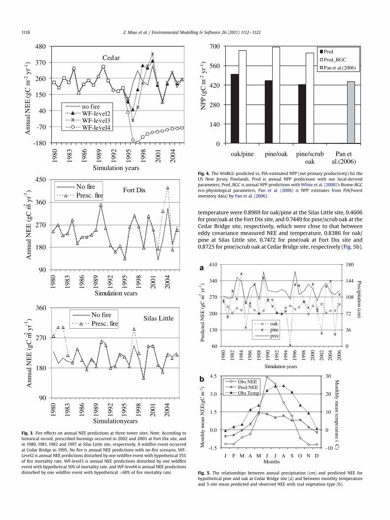
Both prescribed burning and wildfire disturbance had a largeimpact on the model estimates of NEE. While cool seasonprescribed burning increased NEE estimates for 1e2 years after theevent, wildfire disturbance greatly reduced the estimated NEE. Forexample, after spring prescribed burning at the Ft. Dix pine/oak sitein 2002 and 2003, annual NEE estimates in 2002, 2003 and 2004were approximately 25e50% higher than the corresponding NEEestimates for no-fire scenarios (prescribed burning: 174, 323 and416 gCm�2 yr�1, vs. no fire: 131, 211 and 335 gCm�2 yr�1) (Fig. 3).Likewise, similar patterns were observed at the Silas Little oak/pinesite after prescribed burning in 1980, 1981, 1982 and 1997. Theimpact of wildfire disturbance was simulated at the Cedar Bridge

pine/scrub oak site under several different scenarios subsequent toawildfire in 1995. Estimates of annual NEE decreased from a high of230 gCm�2 yr�1 for the no-fire scenario to �26 gCm�2 yr�1 wherethe wildfire mortality rate of 50% was assumed (Fig. 3).

3.2. Estimating the NPP of the New Jersey Pinelands

Using the locally-derived parameters, the WxBGC model NPPpredictions were closely aligned with the Pinelands region-wideestimate made by Pan et al. (2006) based on USDA Forest ServiceFIA (forest inventory and analysis) data (Fig. 4). The NPP predictionsbased on White et al. (2000)’s Biome-BGC eco-physiologicalparameterization were from 25 to 35% higher than the WxBGCsimulations with the locally-derived parameters as well as Pan et al.(2006) (Fig. 4).

Wildfire disturbance considerably reduced the NPP estimateswhile the prescribed burning increased the NPP estimates. Forinstance, the NPP predictions with and without prescribed fireswere 567 and 496 gCm�2 yr�1 for oak/pine at Silas Little site in1981, 351 and 314 gCm�2 yr�1 for pine/oak at Fort Dix site in 2003,respectively. For pine/scrub oak at Cedar Bridge site, NPP estimatesreduced from 543 gCm�2 yr�1 of no wildfire to 249 gCm�2 yr�1

with wildfire disturbance (50% of mortality rate) in 1996(unshown).

3.3. Correlation between the carbon flux simulations andmeteorological driving variables

Annual NEE estimates of the model for pine-dominatedcommunity were more related to precipitation than that of oak-dominated community (Fig. 5a). Without considering firedisturbance, for example, the correlations between annual NEEpredictions and annual precipitation were 0.2850 for pine/scruboak at Cedar Bridge site and 0.0351 for pine/oak at Fort Dix site,respectively, because vegetation cover at Cedar Bridge site hasmore pine components than that at Fort Dix site. We simulatedannual NEE with hypothetical vegetation scenarios, pure pine orpure oak scenarios, based on Cedar Bridge site (not shown). Thecorrelation coefficient between annual NEE predictions andprecipitation increased to 0.5727, while the correlation coefficientbetween annual precipitation and annual NEE predictions forhypothetical pure oak scenario was �0.22.

For three vegetations types, monthly mean NEE predictionswere all significantly associated with temperature. In 2005,correlation coefficients between monthly NEE predictions and

0

140

280

420

560

700

oak/pine pine/oak pine/scrub oak

Pan et al.(2006)

Pred

Pred_BGC

Pan et al.(2006)

mCg(

PP

N-2

ry-1

)

Fig. 4. The WxBGC-predicted vs. FIA-estimated NPP (net primary productivity) for theUS New Jersey Pinelands. Pred is annual NPP predictions with our local-derivedparameters, Pred_BGC is annual NPP predictions with White et al. (2000)’s Biome-BGCeco-physiological parameters, Pan et al. (2006) is NPP estimates from FIA(Forestinventory data) by Pan et al. (2006).

-180

-70

40

150

260

370

4800891

3891

6891

9891

2991

5991

8991

1002

4002

no fireWF-level2WF-level3WF-level4

Simulation years

mCg(

EE

NlaunnA

2-ry

1-)

Cedar

90

180

270

360

450

0891

3891

6891

9891

2991

5991

8991

1002

4002

No firePresc. fire

Simulation years

mCg(

EE

NlaunnA

2-ry

1-) Fort Dix

90

180

270

360

0891

3891

6891

9891

2991

5991

8991

1002

4002

No firePresc. fire

Simulation years

mCg(

EE

NlaunnA

2-ry

1-) Silas Little

Fig. 3. Fire effects on annual NEE predictions at three tower sites. Note: According tohistorical record, prescribed burnings occurred in 2002 and 2003 at Fort Dix site, andin 1980, 1981, 1982 and 1997 at Silas Little site, respectively. A wildfire event occurredat Cedar Bridge in 1995. No fire is annual NEE predictions with no-fire scenario, WF-Level2 is annual NEE predictions disturbed by one wildfire event with hypothetical 35%of fire mortality rate, WF-level3 is annual NEE predictions disturbed by one wildfireevent with hypothetical 50% of mortality rate, and WF-level4 is annual NEE predictionsdisturbed by one wildfire event with hypothetical >60% of fire mortality rate.

Z. Miao et al. / Environmental Modelling & Software 26 (2011) 1112e11221118

temperature were 0.8969 for oak/pine at the Silas Little site, 0.4606for pine/oak at the Fort Dix site, and 0.7449 for pine/scrub oak at theCedar Bridge site, respectively, which were close to that betweeneddy covariance measured NEE and temperature, 0.8386 for oak/pine at Silas Little site, 0.7472 for pine/oak at Fort Dix site and0.8725 for pine/scrub oak at Cedar Bridge site, respectively (Fig. 5b).

60

130

200

270

340

410

0891

2891

4891

6891

8891

0991

2991

4991

6991

8991

0002

2002

4002

6002

0

36

72

108

144

180

oakpineprec

Simulation years

mCg(

EE

Ndetcider

P2-

ry1-)

)mc

(no

itati

pice

rP

-10

0

10

20

30

-1.5

0.0

1.5

3.0

4.5

J F M A M J J A S O N D

Obs NEEPred NEEObs Temp

Months

mCg(

EE

Nnae

mylhtno

M2-)

)C

(er

utar

epme

tna

em

ylht

lno

M

a

b

Fig. 5. The relationships between annual precipitation (cm) and predicted NEE forhypothetical pine and oak at Cedar Bridge site (a) and between monthly temperatureand 3-site mean predicted and observed NEE with real vegetation type (b).

Z. Miao et al. / Environmental Modelling & Software 26 (2011) 1112e1122 1119

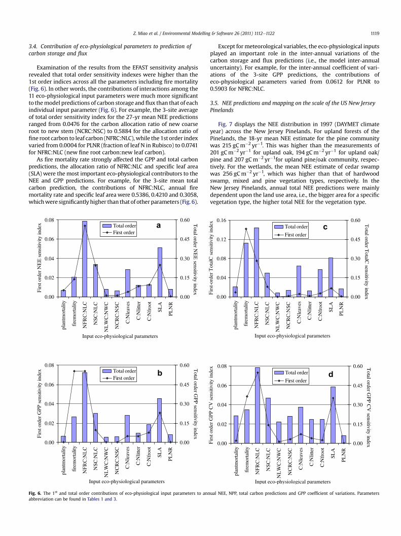
3.4. Contribution of eco-physiological parameters to prediction ofcarbon storage and flux

Examination of the results from the EFAST sensitivity analysisrevealed that total order sensitivity indexes were higher than the1st order indices across all the parameters including fire mortality(Fig. 6). In other words, the contributions of interactions among the11 eco-physiological input parameters were much more significantto themodel predictions of carbon storage and flux than that of eachindividual input parameter (Fig. 6). For example, the 3-site averageof total order sensitivity index for the 27-yr mean NEE predictionsranged from 0.0476 for the carbon allocation ratio of new coarseroot to new stem (NCRC:NSC) to 0.5884 for the allocation ratio offine root carbon to leaf carbon (NFRC:NLC),while the 1st order indexvaried from 0.0004 for PLNR (fraction of leaf N in Rubisco) to 0.0741for NFRC:NLC (new fine root carbon:new leaf carbon).

As fire mortality rate strongly affected the GPP and total carbonpredictions, the allocation ratio of NFRC:NLC and specific leaf area(SLA) were the most important eco-physiological contributors to theNEE and GPP predictions. For example, for the 3-site mean totalcarbon prediction, the contributions of NFRC:NLC, annual firemortality rate and specific leaf area were 0.5386, 0.4210 and 0.3058,whichwere significantly higher than that of other parameters (Fig. 6).

0.00

0.02

0.04

0.06

0.08

ytilatromtnalp

ytilatromerif

CL

N:C

RF

N

CL

N:C

SN

CW

N:C

WL

N

CS

N:C

RC

N

sevaelN:

C

rettilN:

C

toorfN:

C

AL

S

RN

LP

0.00

0.15

0.30

0.45

0.60Total orderFirst order

tivitisnesE

EN

redrotsriF

yxedni

tivit

isne

sE

ENr

edro

lato

Ty

xedn

i

Input eco-physiological parameters

a

0.00

0.02

0.04

0.06

0.08

ytilatromtnalp

ytilatromerif

CL

N:C

RF

N

CL

N:C

SN

CW

N:C

WL

N

CS

N:C

RC

N

sevaelN:

C

rettilN:

C

toorfN:

C

AL

S

RN

LP

0.00

0.15

0.30

0.45

0.60Total orderFirst order

tivitisnesP

PG

redrotsriF

yxedni

tivit

isne

sP

PG

redr

olat

oT

yxe

dni

Input eco-physiological parameters

b

Fig. 6. The 1st and total order contributions of eco-physiological input parameters to annabbreviation can be found in Tables 1 and 3.

Except for meteorological variables, the eco-physiological inputsplayed an important role in the inter-annual variations of thecarbon storage and flux predictions (i.e., the model inter-annualuncertainty). For example, for the inter-annual coefficient of vari-ations of the 3-site GPP predictions, the contributions ofeco-physiological parameters varied from 0.0612 for PLNR to0.5903 for NFRC:NLC.

3.5. NEE predictions and mapping on the scale of the US New JerseyPinelands

Fig. 7 displays the NEE distribution in 1997 (DAYMET climateyear) across the New Jersey Pinelands. For upland forests of thePinelands, the 18-yr mean NEE estimate for the pine communitywas 215 gCm�2 yr�1. This was higher than the measurements of201 gCm�2 yr�1 for upland oak, 194 gCm�2 yr�1 for upland oak/pine and 207 gCm�2 yr�1for upland pine/oak community, respec-tively. For the wetlands, the mean NEE estimate of cedar swampwas 256 gCm�2 yr�1, which was higher than that of hardwoodswamp, mixed and pine vegetation types, respectively. In theNew Jersey Pinelands, annual total NEE predictions were mainlydependent upon the land use area, i.e., the bigger area for a specificvegetation type, the higher total NEE for the vegetation type.

0.00

0.04

0.08

0.12

0.16

ytilatromtnalp

ytilatromerif

CL

N:C

RF

N

CL

N:C

SN

CW

N:C

WL

N

CS

N:C

RC

N

sevaelN:

C

rettilN:

C

toorfN:

C

AL

S

RN

LP

0.00

0.15

0.30

0.45

0.60Total order

First ordertivitisnesClato

Tredro-tsri

Fy

xedni

tivit

isne

sCl

ato

Tred

rola

toT

yxe

dni

Input eco-physiological parameters

c

0.00

0.02

0.04

0.06

0.08

ytilatromtnalp

ytilatromerif

CL

N:C

RF

N

CL

N:C

SN

CW

N:C

WL

N

CS

N:C

RC

N

sevaelN:

C

rettilN:

C

toorfN:

C

AL

S

RN

LP

0.00

0.15

0.30

0.45

0.60Total order

First order

xedniytivitisnes

VC

PP

GredrotsriF xe

dni

ytivit

isne

sV

CP

PG

redr

olat

oT

Input eco-physiological parameters

d

ual NEE, NPP, total carbon predictions and GPP coefficient of variations. Parameters

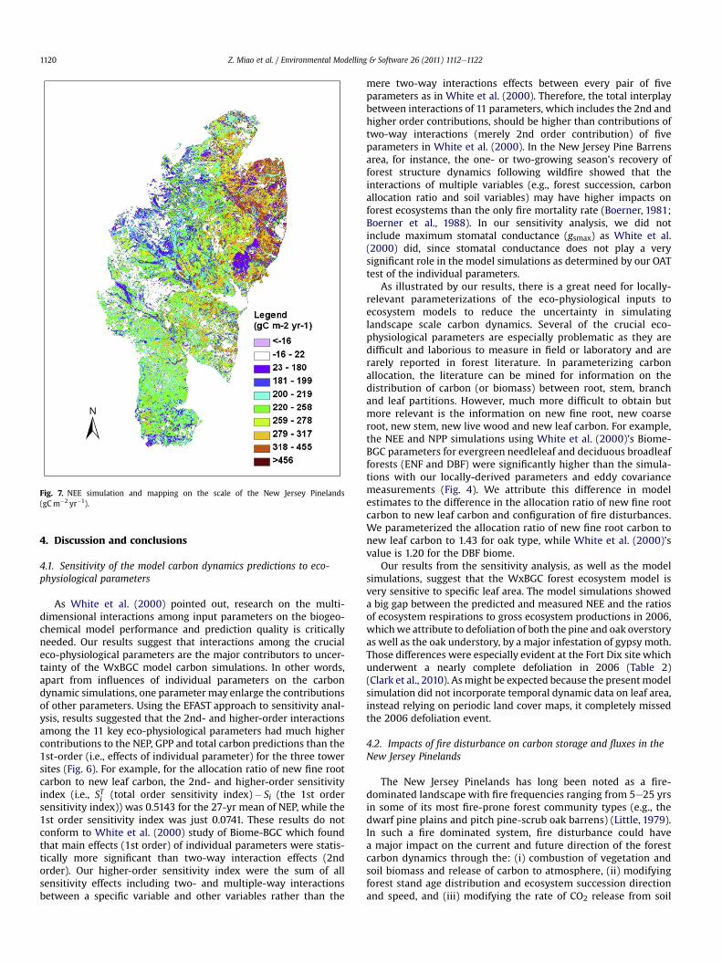
Fig. 7. NEE simulation and mapping on the scale of the New Jersey Pinelands(gCm�2 yr�1).

Z. Miao et al. / Environmental Modelling & Software 26 (2011) 1112e11221120

4. Discussion and conclusions

4.1. Sensitivity of the model carbon dynamics predictions to eco-physiological parameters

As White et al. (2000) pointed out, research on the multi-dimensional interactions among input parameters on the biogeo-chemical model performance and prediction quality is criticallyneeded. Our results suggest that interactions among the crucialeco-physiological parameters are the major contributors to uncer-tainty of the WxBGC model carbon simulations. In other words,apart from influences of individual parameters on the carbondynamic simulations, one parameter may enlarge the contributionsof other parameters. Using the EFAST approach to sensitivity anal-ysis, results suggested that the 2nd- and higher-order interactionsamong the 11 key eco-physiological parameters had much highercontributions to the NEP, GPP and total carbon predictions than the1st-order (i.e., effects of individual parameter) for the three towersites (Fig. 6). For example, for the allocation ratio of new fine rootcarbon to new leaf carbon, the 2nd- and higher-order sensitivityindex (i.e., STi (total order sensitivity index)� Si (the 1st ordersensitivity index)) was 0.5143 for the 27-yr mean of NEP, while the1st order sensitivity index was just 0.0741. These results do notconform to White et al. (2000) study of Biome-BGC which foundthat main effects (1st order) of individual parameters were statis-tically more significant than two-way interaction effects (2ndorder). Our higher-order sensitivity index were the sum of allsensitivity effects including two- and multiple-way interactionsbetween a specific variable and other variables rather than the

mere two-way interactions effects between every pair of fiveparameters as in White et al. (2000). Therefore, the total interplaybetween interactions of 11 parameters, which includes the 2nd andhigher order contributions, should be higher than contributions oftwo-way interactions (merely 2nd order contribution) of fiveparameters in White et al. (2000). In the New Jersey Pine Barrensarea, for instance, the one- or two-growing season’s recovery offorest structure dynamics following wildfire showed that theinteractions of multiple variables (e.g., forest succession, carbonallocation ratio and soil variables) may have higher impacts onforest ecosystems than the only fire mortality rate (Boerner, 1981;Boerner et al., 1988). In our sensitivity analysis, we did notinclude maximum stomatal conductance (gsmax) as White et al.(2000) did, since stomatal conductance does not play a verysignificant role in the model simulations as determined by our OATtest of the individual parameters.

As illustrated by our results, there is a great need for locally-relevant parameterizations of the eco-physiological inputs toecosystem models to reduce the uncertainty in simulatinglandscape scale carbon dynamics. Several of the crucial eco-physiological parameters are especially problematic as they aredifficult and laborious to measure in field or laboratory and arerarely reported in forest literature. In parameterizing carbonallocation, the literature can be mined for information on thedistribution of carbon (or biomass) between root, stem, branchand leaf partitions. However, much more difficult to obtain butmore relevant is the information on new fine root, new coarseroot, new stem, new live wood and new leaf carbon. For example,the NEE and NPP simulations using White et al. (2000)’s Biome-BGC parameters for evergreen needleleaf and deciduous broadleafforests (ENF and DBF) were significantly higher than the simula-tions with our locally-derived parameters and eddy covariancemeasurements (Fig. 4). We attribute this difference in modelestimates to the difference in the allocation ratio of new fine rootcarbon to new leaf carbon and configuration of fire disturbances.We parameterized the allocation ratio of new fine root carbon tonew leaf carbon to 1.43 for oak type, while White et al. (2000)’svalue is 1.20 for the DBF biome.

Our results from the sensitivity analysis, as well as the modelsimulations, suggest that the WxBGC forest ecosystem model isvery sensitive to specific leaf area. The model simulations showeda big gap between the predicted and measured NEE and the ratiosof ecosystem respirations to gross ecosystem productions in 2006,whichwe attribute to defoliation of both the pine and oak overstoryas well as the oak understory, by a major infestation of gypsy moth.Those differences were especially evident at the Fort Dix site whichunderwent a nearly complete defoliation in 2006 (Table 2)(Clark et al., 2010). Asmight be expected because the presentmodelsimulation did not incorporate temporal dynamic data on leaf area,instead relying on periodic land cover maps, it completely missedthe 2006 defoliation event.

4.2. Impacts of fire disturbance on carbon storage and fluxes in theNew Jersey Pinelands

The New Jersey Pinelands has long been noted as a fire-dominated landscape with fire frequencies ranging from 5e25 yrsin some of its most fire-prone forest community types (e.g., thedwarf pine plains and pitch pine-scrub oak barrens) (Little, 1979).In such a fire dominated system, fire disturbance could havea major impact on the current and future direction of the forestcarbon dynamics through the: (i) combustion of vegetation andsoil biomass and release of carbon to atmosphere, (ii) modifyingforest stand age distribution and ecosystem succession directionand speed, and (iii) modifying the rate of CO2 release from soil

Z. Miao et al. / Environmental Modelling & Software 26 (2011) 1112e1122 1121

microbial decomposition. In this present study, we concentratedon fire direct impacts on forest carbon storage and flux (Law et al.,2001; Thornton et al., 2002) and ignored fire effects on ecosystemsuccession and soil microbial activity.

The WxBGC simulations demonstrate that wildfire disturbancetemporarily reduces both NEE and NPP, while spring prescribedburnings increased NPP and NEE. For example, for oak/pine at SilasLittle site where prescribed fire occurred in 1980, 1981, 1982 and1997, annual NEE predictions are increased by 21%, 56%, 45% and20% than that of no prescribed fires, respectively. After prescribedburning, it usually takes 1e2 years for themodel estimates of annualNEE to gradually decline to those where no prescribed burning hasoccurred. Hood et al. (2007) and Battaglia et al. (2008) also reportedthat the success of using prescribed fire to control regenerationdensity in fuel treatments is strongly dependent upon the frequencyand initial time of burning in ponderosa pine (Pinus ponderosa(Dougl.) Laws.). An increase of NEE for post prescribed fire has notbeen observed in the eddy covariance measurements of carbondynamics pre- vs. post-prescribed fire (Clark et al., 2009). Ourmodeled increase is mainly due to the assumption that prescribedfires merely burn litter and coarse woody debris (CWD) while onlyslightly impacting the shrub layer, thus autotrophic and heterotro-phic respiration contributed by litter and CWD is greatly reducedwhile the GPP (from the shrub layer) is only slightly reduced. Witha wildfire carbon burning ratio of 35%, annual NEE predictions forthe pine/scrub oak community were decreased by 80% and 41% atthe first two years after wildfire burning (Fig. 4). Provided thata replacement wildfire disturbance occurred for pine/scrub oak atCedar Bridge in 1995 with carbon burning proportion of above 60%(i.e.,fire carbonburning rate), annualNEEpredictionswere negativefrom 1995 to 2006. In other words, if vegetation canopy iscompletely burned by replacement wildfire, therewill be no carbonassimilation rather respiration from coarse woody debris, litter andsoil will continues and annual NEE will be less than or equal to zeroin the terrestrial ecosystems until newplants sprout and re-grow. Inthis study, we fixed a wildfire carbon combustion loss rate for allforest carbon components and did not take into account differentcombustion rates for different forest components (i.e., foliage, stem,litter, CWD, root, etc.). The model did not consider the change inplant carbon allocation ratio after fire either. In reality, wildfires areknown to burn different forest components unevenly as well aschange plant carbon allocation ratio post-burning (Little, 1979;Clark et al., 2009). For example, Clark et al. (2009, 2010) notedthat during the Warren Grove wildfire in our New Jersey Pinelandsstudy area, the combustion loss rate of understory carbon wassignificantly higher than that of the overstory carbon. To improvethe accuracy and reliability of post-fire simulation of Pinelandscarbon dynamics, improved parameterization based on a widerrange of field measured fire disturbance intensity impacts, e.g.,carbon combustion loss rate of different forest components and fireeffects on forest carbon allocation ratio, are needed. Further modelimprovement and simulations of the long-term effects of firedisturbance on soil microbial activity and ecosystem successionsshould be addressed in the future.

Comparing the improved WxBGC model tool to Biome-BGCversion 4.1.2 for ENF and DBF (White et al., 2000), we found that theway the Biome-BGC model included continuous and homogenousprescribed or wildfire disturbance led to significantly reducedannual NEE estimates. These lower NEE estimates are due to theway the model burns carbon at every time step at every pixel witha specific disturbance intensity, even when the fire intensityparameter is set to a small value. In lieu of this approach, wecoupled stochastic and spatially heterogeneous fire disturbancesinto the model for improved treatment at the landscape level. OurWxBGC model result corroborates previous studies which have

suggested that disturbance type, intensity, frequency and timesince disturbance all exert significant impacts on the net ecosystemexchange of forest carbon and that a forest stand will commonly actas a source of carbon to the atmosphere until respiration fromdecomposers become less than photosynthetic uptake fromregrowing vegetation (Law et al., 2001; Thornton et al., 2002;Goward et al., 2008; Zinck et al., 2010).

4.3. NEE prediction gradients of the US New Jersey Pinelands

The WxBGC model was used to predict and map NEE across theentire Pinelands study area (Fig. 7). Visual examination revealsa high degree of spatial heterogeneity in NEE which are driven byland cover, soil properties and climate of the Pinelands. NEE wasestimated to be generally higher for wetland as compared to uplandforest community types. In addition to the fine scale upland vs.wetland variation, there was subtler between-community differ-ences. Uplands NEE predictions were ranked with pine> pine/oak> oak/pine> oak> shrub> grass. Wetlands NEE predictionswere generally ranked with cedar swamp> lowland pine>mixedhardwood community (white cedar/pine/American holly)> hard-wood swamp. Further field eddy covariance measurements ofwetlands forests are required to better calibrate the modelprediction of wetlands carbon dynamics. Coarser scale geographicgradients are also evident as a result of regional scale trends in soilcharacteristics and climate that also interact with vegetationcommunity composition differences. For example, the northeasternquadrant of the study area is largely dominated by pine and themodel suggests that the pine-dominated community is sensitive toannual precipitation. Higher soil moisture and precipitation in thisportion of the study area result in a higher estimate of NEE. Furtherfield measurements are needed to validate these results.

Acknowledgements

This research was supported by the USDA Forest Service EasternLANDFIRE Prototype and the National Fire Plan. Grateful thanks toDaniel Steinwand and Kurtis Nelson, USGS EROS Data Center, forgenerously sharing the codes for the WxBGC model and toolkits,and Xindi Bian, USFS Eastern Modeling Consortium (EAMC), fortechnical support in the LINUX-based computer cluster. Theauthors thank John Bognar for help in GIS data preparations, JimTrimble for administrating the computer systems, andMoMislivetsfromMissoula USDA RMRS-Fire Sciences Lab for cooperation in theNational LANDFIRE project.

References

Aber, J.D., Driscoll, C.T., 1997. Effects of land use, climate variation and N depositionon N cycling and C storage in northern hardwood forests. Global Biogeochem.Cy. 11, 639e648.

Aber, J.D., Melillo, J.M., McClaugherty, C.A., 1990. Predicting long-term patterns ofmass loss, nitrogen dynamics and soil organic matter formation from initial finelitter chemistry in temperate forest ecosystems. Can. J. Bot 68, 2201e2208.

Battaglia, M.A., Smith, F.W., Shepperd, W.D., 2008. Can prescribed fire be used tomaintain fuel treatment effectiveness over time in Black Hills ponderosa pineforests? For. Ecol. Manage. 256, 2029e2038.

Boerner, R.E.J., 1981. Forest structure dynamics following wildfire and prescribedburning in the New Jersey pine barrens. Am. Midl. Nat. 115, 321e333.

Boerner, R.E.J., Lord, T.R., Peterson, J.C., 1988. Prescribed burning in the oak-pineforest of the New Jersey Pine Barrens: effects on growth and nutrient dynamicsof two Quercus species. Am. Midl. Nat. 120, 108e119.

Buchholz, K., Zampella, R.A., 1987. A 30-year fire history of the New Jersey PinePlains. Bull. New Jersey Acad. Sci. 32, 61e69.

Clark, K.L., Skowronski, N., Hom, J., 2010. Invasive insects impact forest carbondynamics. Glob. Change Biol. 16, 88e101.

Clark, K.L., Gholz, H.L., Castro, M.S., 2004. Carbon dynamics along a chronosequenceof Slash Pine plantations in North Florida. Ecol. Appl. 14, 1154e1171.

Clark, K.L., Skowronski, N., Hom, J., Duveneck, M., Pan, Y., Van Tuyl, S., Cole, J.,Patterson, M., Maurer, S., 2009. Decision support tools to improve the

Z. Miao et al. / Environmental Modelling & Software 26 (2011) 1112e11221122

effectiveness of hazardous fuel reduction treatments in the New Jersey PineBarrens. Int. J. Wildland Fire 18, 3268e3277.

Collins, S.T., Good, R.E., 1987. Canopy-ground layer relationship of Oak-pine forestsin the New Jersey pine barrens. Amer. Midl. Nat 117, 280e288.

Ehrenfeld, J.G., 1981. Nitrogen uptake in lowland plant communities of the NewJersey Pine Barrens (Final Report, 77-27-4669 SNJ DEP, DWR, PinelandsAgreement (10/31/77)). Center for Coastal and Environmental Studies, RutgersUniversity, NJ. pp.1e112.

Ehrenfeld, J.G., Gulick, M., 1981. Structure and dynamics of hardwood swamps inthe New Jersey pine barrens: contrasting patterns in trees and shrubs. Am. J.Bot. 68, 471e481.

Ehrenfeld, J.G., Schneider, J.P., 1991. Chamaecyparis thyoides wetlands and subur-banization: effects on hydrology, water quality and plant community compo-sition. J. Appl. Ecol. 28, 467e490.

Forman, R.T.T., 1979. The Pine Barrens of New Jersey: an ecological mosaic. In:Forman, R.T.T. (Ed.), Pine Barrens: Ecosystem and Landscape. Academic Press,NY, pp. 569e585.

Forman, R.T.T., Boerner, R.E., 1981. Fire frequency and the Pine Barrens of NewJersey. Bull. Torrey Bot. Club 108, 34e50.

Frey, H.C., Patil, S.R., 2002. Identification and review of sensitivity analysis methods.Risk Anal. 22, 553e578.

Gertner, G., 2003. Assessment of computationally intensive spatial statisticalmethods for generating inputs for spatiallyexplicit errorbudgets. FBMIS1, 27e34.

Goward, S.N., Masek, J.G., Cohen, W., Moisen, G., Collatz, G.J., Healey, S.,Houghton, R.A., Huang, C., Kennedy, R., Law, B., Powell, S., Turner, D.,Wulder,M.A.,2008. Forest disturbance and North American carbon flux. EOS 89, 1e106.

Havens, A.V., 1979. Climate and microclimate of the New Jersey Pine Barrens. In:Forman, R.T.T. (Ed.), Pine Barrens: Ecosystem and Landscape. Academic Press,New York, pp. 113e131.

Hood, S.M., McHugh, C.W., Ryan, K.C., Reinhardt, E., Smith, S.L., 2007. Evaluation ofa post-fire tree mortality model for western USA conifers. Int. J. Wildland Fire16, 679e689.

Keane, R.E., Rollins, M.G., McNicoll, C.H., Parsons, R.A., 2002. Integrating ecosystemsampling, gradient modeling, remote sensing, and ecosystem simulation tocreate spatially explicit landscape inventories. USDA For. Serv. Gen. Tech. Rep.RMRS-GTR-92. pp. 1e61.

Lane, P.N.J., Feikema, P.M., Sherwin, C.B., Peel, M.C., Freebairn, A.C., 2010. Modellingthe long term water yield impact of wildfire and other forest disturbance inEucalypt forests. Environ. Modell. Softw. 25, 467e478.

Lathrop, R., Kaplan, M.B., 2004. New Jersey land use/land cover update: 2000e2001.New Jersey Department of Environmental Protection, Trenton, New Jersey.

Law, B.E., Thornton, P.E., Irvine, J., Anthoni, P.M., Vantuyl, S., 2001. Carbon storageand fluxes in ponderosa pine forests at different developmental stages. Glob.Change Biol. 7, 755e777.

Little, S., 1979. Fire and plant succession in the New Jersey Pine Barrens. In:Forman, R.T.T. (Ed.), Pine Barrens: Ecosystem and Landscape. Academic Press,NY, pp. 297e331.

Makler-Pick, V., Gal, G., Gorfine, M., Hipsey, M.R., Carmel, Y., 2011. Sensitivityanalysis for complex ecological models: a new approach. Environ. Modell.Softw. 26, 124e134.

Matsushita, B., Xu, M., Chen, J., Kameyama, S., Tamura, M., 2004. Estimation ofregional net primary productivity (NPP) using a process-based ecosystemmodel: how important is the accuracy of climate data? Ecol. Model. 178,371e388.

McCormick, J., 1979. The vegetation of the New Jersey pine barrens. In:Forman, R.T.T. (Ed.), Pine Barrens: Ecosystem and Landscape. Academic Press,NY, pp. 229e243.

McCormick, J., Jones, L., 1973. The Pine Barrens: Vegetation Geography. ResearchReport Number 3, New Jersey State Museum, pp. 76.

Melin, E., 1930. Biological decomposition of some types of litter from NorthAmerican forests. Ecology 16, 72e101.

Miao, Z., Li, C., 2007. Biomass estimates for major boreal forest species in west-central Canada. NRCan Can. For. Serv. Inf. Rep. FI-X-002. pp. 1e37.

Miao, Z., Li, C., 2010. Predicting tree growth dynamics of boreal forest in response toclimate change. In: Li, C., Lafortezza, R., Chen, J. (Eds.), Landscape Ecology andForest Management: Challenges and Solutions in a Changing Globe. Springer-HEP Publisher (chapter 8).

Miao, Z., Trevisan, M., Capri, E., Padovani, L., Del Re, A.A.M., 2004. Uncertaintyassessment of the model RICEWQ in northern Italy. J. Environ. Qual. 33,2217e2228.

Miao, Z., Xu, M., Lathrop, R.G., Wang, Y., 2009. Comparison of A-Cc curve fittingmethods in determining maximum Rubisco carboxylation rate (Vcmax), poten-tial light saturated electron transport rate (Jmax) and leaf dark respiration (Rd).Plant Cell Environ. 32, 109e122.

Moncrieff, J.B., Massheder, J.M., Verhoeh, A., Elbers, J., Heusinkveld, B., Scott, S.,de Bruin, H., Kabat, P., Jarvis, P.J., 1997. A system to measure surface fluxes ofenergy, momentum and carbon dioxide. J. Hydrol. 188e189, 589e611.

Olsvig, L.S., 1980. A comparative study of northeastern pine barrens vegetation.Ph.D. dissertation. Cornell University, Ithaca, NY, pp. 479.

Pan, Y., Birdsey, R., Hom, J., McCullough, K., Clark, K., 2006. Improved estimates ofnet primary productivity from MODIS satellite data at regional and local scales.Ecol. Appl. 16, 125e132.

Reich, P.B., Kloeppel, B.D., Ellsworth, D.S., Walters, M.B., 1995. Different photo-synthesisenitrogen relations in deciduous hardwood and evergreen coniferoustree species. Oecologia 104, 24e30.

Reichstein, M., Falge, E., Baldocchi, D., Papale, D., Aubinet, M., Berbigier, P.,Bernhofer, C., Buchmann, N., Gilmanov, T., Granier, A., Grünwald, T.,Havránková, K., Ilesniemi, H., Janous, D., Knohl, A., Laurila, T., Lohila, A.,Loustau, D., Matteucci, G., Meyers, T., Miglietta, F., Ourcival, J.M., Pumpanen, J.,Rambal, S., Rotenberg, E., Sanz, M., Tenhunen, J., Seufert, G., Vaccari, F., Vesala, T.,Yakir, D., Valent ini, R., 2005. On the separation of net ecosystem exchange intoassimilation and ecosystem respiration: review and improved algorithm. Glob.Change Biol. 11, 1e16.

Rollins, M.G., Keane, R.E., Zhu, Z., Menakis, J.P., 2006. An overview of the LANDFIREprototype project (Chapter 2). USDA For. Serv. Gen. Tech. Rep. RMRS-GTR-175.pp. 5e43.

Ruimy, A., Jarvis, P.G., Baldocchi, D.D., Saugier, B., 1995. CO2 fluxes over plantcanopies and solar radiation: a review. Adv. Ecol. Res. 26, 1e68.

Running, S.W., Gower, S.T., 1991. FOREST-BGC, a general model of forest ecosystemprocesses for regional applications. II. Dynamic carbon allocation and nitrogenbudgets. Tree Physiol. 9, 147e160.

Saltelli, A., 2002. Sensitivity analysis for importance assessment. Risk Anal. 22,579e590.

Saltelli, A., Annoni, P., 2010. How to avoid a perfunctory sensitivity analysis. Environ.Modell. Softw. 25, 1508e1517.

Saltelli, A., Bolado, R., 1998. An alternative way to computer Fourier amplitudesensitivity test (FAST). Comput. Statist. Data Anal 26, 445e460.

Saltelli, A., Tarantola, S., Campolongo, F., 2000. Sensitivity analysis as an ingredientof modeling. Statist. Sci. 15, 377e395.

Scherzer, A.J., Hom, J., 2008. Database of Physiological Parameters for CommonSpecies of Eastern Hardwood Forests. USDA Forest Service, Northern GlobalChange Research Program, Newtown Square, PA.

Sitch, S., Smith, B., Prentice, I.C., Arneth, A., Bondeau, A., Cramer, W., Kaplan, J.O.,Levis, S., Lucht, W., Sykes, M.T., Thonicke, K., Venevsky, S., 2003. Evaluation ofecosystem dynamics, plant geography and terrestrial carbon cycling in the LPJdynamic global vegetation model. Glob. Change Biol 9, 161e185.

Skowronski, N., Clark, K., Nelson, R., Hom, J., Patterson, M., 2007. Remotely sensedmeasurements of forest structure and fuel loads in the Pinelands of New Jersey.Remote Sens. Environ. 108, 123e129.

Tedrow, J.C.F., 1986. Soils of New Jersey. New Jersey Agricultural Experiment StationPublication A-15134-1-82. Krieger Publishing Co., Malabar, FL.

Thornton, P.E., Hasenauer, H., White, M.A., 2000. Simultaneous estimation of dailysolar radiation and humidity from observed temperature and precipitation: anapplication over complex terrain in Austria. Agri. For. Meteorol. 104, 255e271.

Thornton, P.E., Law, B.E., Gholz, H.L., Clark, K.L., Falge, E., Ellsworth, D.S.,Goldstein, A.H., Monson, R.K., Hollinger, D., Falk, M., Chen, J., Sparks, J.P., 2002.Modeling and measuring the effects of disturbance history and climate oncarbon and water budgets in evergreen needleleaf forests. Agri. For. Meteorol.113, 185e222.

Thornton, P.E., Running, S.W., 1999. An improved algorithm for estimating incidentdaily solar radiation from measurements of temperature, humidity, andprecipitation. Agri. For. Meteorol. 93, 211e228.

Thornton, P.E., Running, S.W., White, M.A., 1997. Generating surfaces of dailymeteorological variables over large regions of complex terrain. J. Hydrol. 190,214e251.

Updegraff, K., Zimmerman, P.R., Kozak, P., Chen, D.G., Price, M., 2010. Estimating theuncertainty of modeled carbon sequestration: the GreenCert_ system. Environ.Modell. Softw. 25, 1565e1572.

Wang, D., 1984. Fire and nutrient dynamics in a pine-oak forest ecosystem in theNew Jersey Pine Barrens. Ph.D. dissertation. Yale University, New Haven, CT. pp.1e217.

Wang, J., Chen, J., Ju, W., Li, M., 2010. IA-SDSS: A GIS-based land use decisionsupport system with consideration of carbon sequestration. Environ. Modell.Softw. 25, 539e553.

Walther, G.R., Post, E., Convey, P., Menzel, A., Parmesank, C., Beebee, T.J.C.,Fromentin, J.M., Hoegh-Guldberg, O., Bairlein, F., 2002. Ecological responses torecent climate change. Nature 416, 389e395.

White, M.A., Thornton, P.E., Running, S.W., Nemani, R.R., 2000. Parameterizationand sensitivity analysis of the BIOMEeBGC Terrestrial Ecosystem Model: netprimary production controls. Earth Interact. 4, 1e85.

Whittaker, R.H., 1962. Net production relations of shrubs in the Great SmokyMountains. Ecology 43, 357e377.

Whittaker, R.H., Woodwell, G.M., 1969. Structure, production and diversity of theoak-pine forest at Brookhaven, New York. J. Ecol. 57, 155e174.

Whittaker, R.H., Woodwell, G.M., 1968. Dimension and production relations of treesand shrubs in the Brook forest, New York. J. Ecol. 56, 1e25.

Wood, O.M., 1937. The interception of precipitation in an oak-pine forest. Ecology18, 251e254.

Woodwell, G.M., Whittaker, R.H., Houghton, R.A., 1975. Nutrient concentrations inplants in the Brookhaven oak-pine forest. Ecology 56, 318e332.

Wullschleger, S.T., 1993. Biochemical limitations to carbon assimilation in C3plantseA retrospective analysis of the A-Ci curves from 109 species. J. Exp. Bot44, 907e920.

Xu, M., Lathrop, R., Miao, Z., 2007. Plant physiological response of indicator speciesto water stress in the New Jersey Pinelands. Final report of Physiological StressIndicators task of the Kirkwood-Cohansey Project, 1e61.

Yang, J., 2011. Convergence and uncertainty analyses in Monte-Carlo based sensi-tivity analysis. Environ. Modell. Softw. 26, 444e457.

Zinck, R.D., Johst, K., Grimm, V., 2010. Wildfire, landscape diversity and the Dros-seleSchwabl model. Ecol. Model. 221, 98e105.