SIMO Extension of the Algorithm of Mode Isolation

M. S. Allen, and J. H. GinsbergThe G. W. Woodruff School of Mechanical Engineering

Georgia Institute of TechnologyAtlanta, GA 30332-0405

October 10, 2003

Abstract

Many multi-degree-of-freedom (MDOF) modal analysis algorithms make use of a stabilization diagram tolocate system modes. The algorithm of mode isolation (AMI) provides an alternative approach in which modesare identified and subtracted from the data one at a time. An iterative procedure then refines the initial estimate.Previous work has shown that AMI gives good results when compared to other MDOF algorithms. This workpresents an extension of AMI in which the frequency response functions (FRFs) from all measurement points areconsidered simultaneously, resulting in global estimates for natural frequencies and damping ratios, and consistentmode vectors. A linear-least-squares, frequency domain, global, SIMO, SDOF fitting algorithm is derived andtested using noise contaminated analytical data. Comparisons with the rational fraction polynomial algorithm(RFP-SIMO) and the stochastic subspace identification algorithm (SSI) show that AMI performs favorably.

1 Nomenclature

HjP (ω)

½FRF for displacement jdue to excitation P

Hc Composite FRF

{AP,r} Modal residue vector forthe rth mode driven at P

λr rth eigenvalue

{φr} rth displacement mode vector(Normalized)

ωr rth natural frequencyζr rth modal damping ratio{q} Generalized coordinates

{ψr} rth state space mode vector(Normalized)

w Transverse displacementθ Torsional rotationω Drive frequency

2 Introduction

Allemang [1] stated: “The estimation of an appropriate model order is the most important problem encounteredin modal parameter estimation.” Model order determination comprises much of the user interaction involved inexperimental modal analysis [2].

The objectives in experimental modal analysis differ from those in general system identification, in that the goal ismeaningful modes of vibration, rather than matching of input and output data. Virtually all MDOF identificationalgorithms return a number of computational modes intermixed with the true system modes. There are twoconsiderations in findi ng an appropriate mo del order: Finding the ord er th at give s th e mos t accurate mo dalparameters for the true system modes, and distinguishing true system modes from computational ones.

Plots of singular values (as in ERA or SSI for example [3],[4],[5]) or error charts [2] [1] may suggest a model order thatresults in modal parameters that are accurate enough for many purposes, though optimality has not been studied.Careful inspection of a stabilization diagram will give an indication of the magnitude of variance from one modelorder to the next, but bias errors that are stable relative to model order are more difficult to detect. In this work,stabilization diagrams generated by the Stochastic Subspace Algorithm (SSI) will be examined for an indication ofbias and variance errors. It will be shown that the SSI algorithm tends to give a false sense of security regarding theaccuracy of the modal parameters. Furthermore, the best accuracy can only be obtained if significant computationalresources are available.

The stabilization diagram is also the primary tool for distinguishing computational modes from true system modes.There are a number of tools available to assist in this. Goethals and De Moor [6] found that energy could be usedto distinguish many of the spurious modes. Verboven et al [7] used pole characteristics as well as properties ofthe stabilization diagram, such as the variation in a pole’s frequency from one model order to the next, to detectspurious modes. While these represent substantial aides, an absolute criteria for detecting spurious modes for ageneral problem has not been developed. A common approach is to use a stabilization diagram, combined withmode indicator functions, such as the complex mode indicator function (CMIF), to manually extract true modesfrom the MDOF algorithm’s output. In some frequency ranges, stable modes may not be visible [8]. Furthermore,none of these methods assess the effect of computational modes on the accuracy of true system modes.

The algorithm of mode isolation (AMI) offers a different perspective on the problem of finding the true modes ofa system. In AMI, modes are extracted one at a time, and then subtracted from the data. In this process theimportance of each mode in the fit is clearly visible. The number of true modes in the data set is then taken tobe the number of modes that must be fit to the data to reduce it to noise. An iterative procedure then refines theinitial estimate. The resulting MDOF fit does not include any spurious or computational modes. Previous work [9],[10] has shown that AMI gives substantially more accurate results when compared to some other MDOF algorithmsthat fit a system with a number of model orders and then later try to extract meaningful results. Furthermore, theconditions under which the problem is ill conditioned are revealed.

Because modes are identified one at a time, only a single degree of freedom fit is needed, which makes the algorithmcomputationally efficient, with small workspace requirements. AMI can be used whenever an FRF can be representedas a sum of poles with associated residues. For example, Joh and Lee [11] suggested a procedure similar to AMI tosimplify the identification of rotordynamic systems. Another possible extension might be to aid in finding frequencydomain models for viscoelastic systems, as in [12].

The primary new feature of the present work is its implementation of a refined technique for fitting individual modes.Ginsberg et al [13] derived a linear-least-squares fitting procedure that is exact for noise-free data. That techniqueused only a single FRF. The present work extends the previous development to obtain a set of parameters thatsimultaneously best fit all FRFs.

3 The Algorithm of Mode Isolation

AMI was first presented by Drexel and Ginsberg [9], although it was previously suggested by Joh and Lee [11].Improvements to the algorithm and the results of test problems are documented in [14], [15], [16], [13] and [17]. AMIis based upon the recognition that the FRF data to be fit is a superposition of individual modal contributions. AMIidentifies each mode individually, and then subtracts its contribution from the data. Once all of the modes havebeen subtracted, only noise remains, thereby identifying the model order as the number of modes subtracted beforethe data is reduced to noise. An iterative procedure is then used to refine the initial estimate in order to accountfor overlapping contributions of adjacent modes. The algorithm also provides a self-correcting check that the initialidentification of the number of contributory modes is correct. Although AMI begins like the SDOF methods usedhistorically, in which the contribution of modes other than the one in focus is neglected, the iterative proceduremakes it an MDOF algorithm that accounts for coupling between modes.

The procedure will be described briefly here. The discussion will focus on a new, global, SIMO implementation.Differences between this and the SISO implementation of AMI will be highlighted. The data analyzed in AMIconsists of the frequency response of all measurement degrees of freedom (DOF) to a harmonic force at the P thmeasurement DOF. (By reciprocity this is equivalent to the response of the P th DOF to a force applied to eachmeasurement DOF sequentially.) It is assumed that the system dynamics can be represented by the familiar second

order matrix differential equation[M ] {q̈}+ [C] {q̇}+ [K] {q} = {F} (1)

where {q}, [M ], [C], and [K] are the generalized coordinate vector, and symmetric mass, damping and stiffnessmatrices respectively each of dimensions N×N . The force vector {F} is zero everywhere except the P th generalizedcoordinate (or drive point) for a SIMO experiment. When eq. (1) is put into state space form by stacking {q} above{q̇}, the following symmetric generalized eigenvalue problem results

[[R]− λ [S]] {ψ} = {0}where {ψ} is an arbitrarily scaled mode vector and [R] and [S] are defined as follows.

[R] =

·[0] − [K]− [K] − [C]

¸, [S] =

· − [K] [0][0] [M ]

¸It can be shown that underdamped modes result in a pair of complex conjugate eigenvalues λr whose respectivemode vectors {ψr} are also complex conjugates [18]. The mass normalized mode matrix can then be expressed as

[Ψ] =£ {ψ1} {ψ2} · · · ¤ = · [φ] [φ∗]

[λ] [φ] [λ∗] [φ∗]

¸where [λ] is a diagonal matrix of eigenvalues having positive imaginary parts and [φ] is the displacement portion ofthe mode matrix. The frequency response function {HP (ω)} is the ratio of the complex response amplitude of eachgeneralized displacement to the drive force amplitude. It is related to the state space modal properties by

{HP (ω)} =NXr=1

{AP,r}iω − λr

+

©A∗P,r

ªiω − λ∗r

(2)

{AP,r} = λr {φr}φPrwhere λr and {φr} are the complex eigenvalue and complex normalized eigenvector of the rth mode of vibration.The notation φPr signifies the P th element of the rth mode vector, or the Prth element of the displacement portionof the modal matrix, and {AP,r} is the P th column of the residue matrix for mode r. The eigenvalue is relatedto the natural frequency and damping ratio by: λr = −ζrωr ± ωr

¡1− ζ2r

¢1/2where ωr and ζr are the rth natural

frequency and damping ratio.

AMI proceeds in two stages: Subtraction and Isolation. These stages will be described for the global SIMOimplementation, though the overall procedure is similar to the SISO implementation described in previous papers.

3.1 Subtraction StageAMI begins with the subtraction stage, in which modes are subtracted from the experimental data one at a time.The algorithm starts by considering the dominant mode, located as the highest peak of the composite FRF, wherethe composite FRF is defined as the sum of the magnitude of the FRFs for all response points,

Hc (ω) =

NoXj=1

|HjP (ω)| (3)

with No being the number FRFs. The SISO implementation of AMI operated successively on a single FRF, andthus did not consider a composite FRF.

Data in the vicinity of the peak in the composite FRF is sent to an SDOF fitting algorithm (described subsequently)that returns the eigenvalue and mode vector that best fit the dominant mode in all FRFs. The number of datapoints around the peak that are fit is a compromise between averaging out noise (more points) and reducing thecontribution of other modes (fewer points). For the problems presented in this paper the half power points wereused, defined as all points near the peak such that

Hc (ω) > α ∗max (Hc (ω)) (4)

where α = 0.707.

An FRF model for the fit mode is then constructed using eq. (2), and the fit mode is subtracted from the FRF data.This brings the mode having the next highest peak into dominance. This mode is also identified and subtractedfrom the data. The process continues until the composite FRF shows no coherent peaks suggestive of the presenceof additional modes. Presently, this is determined by visual inspection of the data.

3.2 Mode Isolation StageOnce all of the modes of the system have been approximated, the estimate for each mode is refined through aniterative procedure. At this stage the algorithm proceeds through the modes in the sequence of their dominance inthe composite FRF. The contributions of all modes except for the one in focus are subtracted from the FRF data.This leaves only the experimentally measured contribution of the mode in focus, as well as noise and any errors thatmay exist in the fit of the other modes. The mode in focus is then re-fit using the SDOF fitting algorithm. Atthis point, the data essentially contains only one mode, so an SDOF fit yields an improved estimate of the currentmode’s parameters. Also, because the contribution of all other modes has presumably been removed from the data,the fitting algorithm can now consider more data around the peak, further minimizing the effects of noise. Careshould be taken however. Because of the limited resolution of sensors and data acquisition equipment, data veryfar from the peak may not be reliable. For the problems presented subsequently, the criteria in eq. (4) was appliedwith α = 0.5, (fitting the data above the quarter-power points rather than the half power points.) In [13], Ginsberget al found that this was optimum for a single FRF contaminated with random, white noise.

The model is then updated with the modal parameters fitting the mode in focus, and the algorithm proceeds tothe next mode. A cycle through all identified modes constitutes one iteration. Typically only a few iterations arerequired. Computations cease when convergence criteria for the eigenvalues and residues have been met.

3.3 SIMO SDOF Fitting AlgorithmThe extension of AMI from SISO to SIMO is achieved by expanding the data set and vectorizing the algorithm. Itinvokes a (non-iterative) linear-least-squares fit. Considering only the rth mode in eq.(2), and placing the two termsassociated with this mode on a common denominator yields

{HP (ω)} = 2 iωRe ({AP})−Re ({AP}λ∗)

|λ|2 − ω2 − 2iωRe (λ) (5)

Note that the subscript r has been dropped because only one mode is considered. Clearing the denominator in eq.(5) and breaking the result into real and imaginary parts then leads to

Re [{HP (ω)}]³|λ|2 − ω2

´+ 2ω Im [{HP (ω)}] Re (λ) = −2Re ({AP}λ∗) (6)

Im [{HP (ω)}]³|λ|2 − ω2

´− 2ωRe [{HP (ω)}] Re (λ) = 2ωRe ({AP }) (7)

The resulting system of equation is linear in |λ|2, Re (λ) , and in the vector variables: Re ({AP }) , and Re ({AP}λ∗).In matrix form this can be expressed as:

·Re {HP (ω)} 2ω Im {HP (ω)} 2 [I] [0]Im {HP (ω)} −2ωRe {HP (ω)} [0] −2ω [I]

¸|λ|2Re (λ)Re {AP }

Re ({AP }λ∗)

=

½ω2Re {HP (ω)}ω2 Im {HP (ω)}

¾(8)

where the identity matrices [I] and zero matrices [0] are all of dimensions No × No. The matrix on the left handside and the vector on the right hand side of eq. (8) are both known at a number of discrete frequencies. These areevaluated at L > 1 discrete frequencies near a resonance and stacked resulting an the overdetermined linear systemdenoted as follows.

[α](2NoL)×(2No+2){x}(2No+2)×1 = {β}(2NoL)×1 (9)

The parameters {x} that minimize the squared fit error in eq. (9) are found to be

{x} =³[α]

T[α]´−1 ³

[α]T {β}

´(10)

The solution to eq. (10) can be made more computationally efficient by expressing the elements of the products[α]

T[α] and [α]T {β} in terms of the raw data, rather than actually forming [α] and {β} and evaluating the products.

Furthermore, the product matrices can be computed directly with minimal operations because a number of elementsof [α] and {β} cancel or are multiplied by zero when the products are evaluated. The overall fitting process isvery efficient and requires little computation time. Because a large number of frequencies are typically used, (i.e.L >> 1), this results in a substantial reduction in the size of the fitting matrix.

The global SIMO algorithm described above resembles the rational fraction polynomial (RFP) method, restricted toa single degree of freedom. Despite this similarity, the differences in computation time and performance are great.The RFP algorithm needs orthogonal polynomials to improve numerical conditioning. The polynomials must beorthogonal with respect to the data set, and so significant computational effort is involved in finding them. Eventhen, ill conditioning occurs as the model order, and hence the powers in the polynomials, increase. Because theglobal SIMO algorithm above is limited to a single degree of freedom, the highest power of ω that occurs is ω2, soill conditioning is not an issue. Also, because only SDOF fits are used in the fitting process, memory does not limitthe maximum number of modes that can be fit as with many MDOF methods (SSI or ERA for example). This mayeliminate the need to analyze data in blocks or to analyze band-pass filtered subsets of data, as is often done withpopular MDOF algorithms.

The performance of AMI-SIMO relative to the rational fraction polynomial and stochastic subspace algorithms willbe evaluated in later sections through the use of an analytical test problem that allows for a definite assessment ofaccuracy.

4 Test Problem: Cantilevered Frame

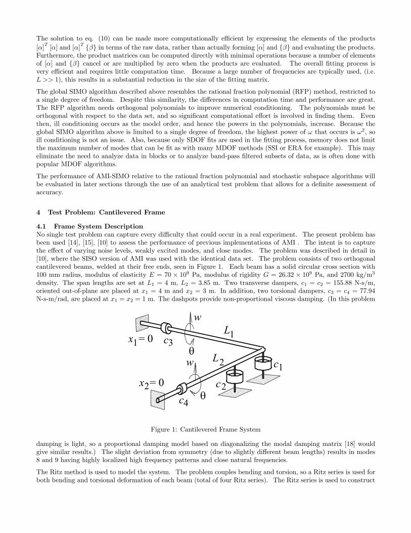
4.1 Frame System DescriptionNo single test problem can capture every difficulty that could occur in a real experiment. The present problem hasbeen used [14], [15], [10] to assess the performance of previous implementations of AMI . The intent is to capturethe effect of varying noise levels, weakly excited modes, and close modes. The problem was described in detail in[10], where the SISO version of AMI was used with the identical data set. The problem consists of two orthogonalcantilevered beams, welded at their free ends, seen in Figure 1. Each beam has a solid circular cross section with100 mm radius, modulus of elasticity E = 70 × 109 Pa, modulus of rigidity G = 26.32 × 109 Pa, and 2700 kg/m3density. The span lengths are set at L1 = 4 m, L2 = 3.85 m. Two transverse dampers, c1 = c2 = 155.88 N-s/m,oriented out-of-plane are placed at x1 = 4 m and x2 = 3 m. In addition, two torsional dampers, c3 = c4 = 77.94N-s-m/rad, are placed at x1 = x2 = 1 m. The dashpots provide non-proportional viscous damping. (In this problem

c1

22

θc3

c4

L

2

1

L

w

w

θc

x = 01

x = 0

Figure 1: Cantilevered Frame System

damping is light, so a proportional damping model based on diagonalizing the modal damping matrix [18] wouldgive similar results.) The slight deviation from symmetry (due to slightly different beam lengths) results in modes8 and 9 having highly localized high frequency patterns and close natural frequencies.

The Ritz method is used to model the system. The problem couples bending and torsion, so a Ritz series is used forboth bending and torsional deformation of each beam (total of four Ritz series). The Ritz series is used to construct

Mode Re{λ} Im{λ} Dampζ ∗ 100

1 -0.656461 68.0047 0.972 -0.164031 265.912 0.063 -0.482573 386.324 0.124 -0.267046 829.451 0.035 -0.793483 1033.75 0.086 -0.610694 1697.01 0.047 -3.1205 1937.89 0.168 -18.7961 2479.67 0.769 -18.1254 2510.98 0.7210 -5.34622 2995.66 0.1811 -5.21094 3380.04 0.15

Table 1: Eigenvalues for First 11 Modes

the system matrices, from which the state-space modal properties of the system are found. For a more detaileddescription of the system and modeling, see [14], [15]. Also, this problem is presented as an exercise in Ginsberg[18], though with different system parameters. The Ritz analysis results in a set of analytical modal parameters.The eigenvalues for the lowest 11 modes are shown in Table 1.

Truncation of each Ritz series at 11 terms was found to yield convergent results for the lowest 21 modes. Thesewere used to construct the time domain response due to a unit impulsive force in the first beam, one meter fromthe clamped support. (The unconverged modes were at frequencies well beyond the range of interest.) Using theRitz series, the displacement and rotation as a function of time at 7 points on the structure due to the impulsiveforce were obtained. The resulting response vector {y (t)} contains both displacements and rotations at locationsone meter apart,

{y (t)} = [w1 w2 w3 w4 θ1 θ2 θ3 θ4 w5 w6 w7 θ5 θ6 θ7 θ8]T (11)

where the first 8 elements are measured on the first beam and the last 7 elements are measured on the second beam.

The analytical responses were sampled, and then noise contaminated by adding zero-mean, normally distributedwhite noise scaled to have a standard deviation of 1% of the maximum of each impulse response. The noisecontaminated impulse responses were then transformed to frequency response functions (FRFs) via a Fast FourierTransform (FFT). The sample rate and sample time were chosen to satisfy the Nyquist criterion and minimizeleakage in the FFT.

4.1.1 Response DataThe resulting noise-contaminated and clean FRFs for the drive point (the first measurement DOF) are shown inFigures 2 and 3. A zoom view is included, which focuses on the response of the close modes 8 and 9.

ω (rad/s)

G11

(ω)

0 500 1000 1500 2000 2500 3000 350010-9

10-8

10-7

10-6

10-5

2200 2400 2600 280010-9

10-8

10-7

Figure 2: Noisy displacement FRF at x = 1 m on beam 1.

Eleven modes are present in the frequency band of interest. The high frequency modes (8-11) are barely visible in

ω (rad/s)

G11

(ω)

0 1000 2000 300010-9

10-8

10-7

10-6

10-5

2200 2400 2600 280010-9

10-8

10-7

Figure 3: Clean displacement FRF at x = 1 m on beam 1.

ω (rad/s)

G(1

3)1(ω

)

0 500 1000 1500 2000 2500 3000 350010-9

10-8

10-7

10-6

10-5

2200 2400 2600 280010-8

10-7

10-6

Figure 4: Noisy rotation FRF at x = 2 m on beam 2.

the noise-contaminated data. In contrast, the higher frequency modes are fairly well represented in the rotationdata, as evidenced in Figure 4. Only a single peak is evident due to modes 8 and 9. These figures are typical of allof the data. There is a large range in effective noise amplitude in the vicinity of the resonance peaks. The signalto noise ratios at the peaks of the FRFs range from 60-40 dB for the dominant, low frequency modes, and from 20dB to negative for the weakly excited, high frequency modes.

4.2 Analysis with Peak-Picking MethodTo aid in assessing the results that follow, the peak-picking and half-power bandwidth methods were used on thecomposite FRF to find the natural frequencies and damping ratios of the system modes, which yields estimatedeigenvalues. Because no peak is evident in the composite FRF in the vicinity of mode 8, it was missed. The averageof the absolute value of the errors in the real and imaginary parts of the eigenvalues for the first seven modes were10% and 0.039% respectively. These were dominated by errors in modes 1 and 4 because of the coarseness of theFRF in the vicinity of these peaks. Without these modes the average errors drop to 2.3% and 0.010%. For modes9-11 the average errors are, 11% and 0.025%.

4.3 Analysis with SIMO-AMIThe FRFs for frequencies from 0 to 3800 rad/s (8589 data points per FRF) were analyzed with AMI in an interactivemode. After each subtraction step, a user examined the composite FRF and decided whether to continue to look formore modes. Ten modes were identified in the subtraction stage of AMI. Mode 8 is buried in noise in the compositeFRF after all other modes were removed, so it was missed completely.

For illustrative purposes, the composite FRF is plotted against the fit composite for the last few subtraction steps.Figure 5 shows the composite residual versus fit for the 8th mode that was found (analytical mode 10). The pointsused in the fit (the half power points) are accented as well. The residual after removing the 8th mode and the fiton the 9th mode (analytical mode 9) are shown in Figure 6. Figure 7 shows the next subtraction step. Figure 7also illustrates the severe effect of the noise on the data away from resonance, as only the peak data resembles thereconstructed response.

0 1000 2000 3000 400010

-10

10-9

10-8

10-7 Composite of Residual vs. Composite of Fit

Frequency (rad/s)

Mag

nitu

de o

f Com

posi

te F

RF

Comp|FRF|Comp|Fit|Points Used

Figure 5: AMI - Composite Residual FRF and single mode fit at the eighth subtraction step, which identifiesanalytical Mode 10.

0 1000 2000 3000 400010

-9

10-8

10-7 Composite of Residual vs. Composite of Fit

Frequency (rad/s)

Mag

nitu

de o

f Com

posi

te F

RF

Comp|FRF|Comp|Fit|Points Used

Figure 6: AMI - Composite Residual FRF and single mode fit at the ninth subtraction step, which identifies analyticalMode 9.

In Figure 7 the data seems to have been reduced to noise, except for the peak to which the 11th analytical modeis fit. A very small bump is evident in the data where the 8th mode should be. The presence of mode 8 in thedata has adversely affected the estimation of mode 9, causing AMI to overestimate the residue at the response pointswhere mode 8 is active and reducing the accuracy of the 9th eigenvalue. This occurs because AMI is trying to fita single mode to the response of two modes. If mode 8 were identified during the subtraction stage, these errorscould be eliminated in the mode isolation stage, when the contributions of other modes are accounted for. Becausemode 8 is not identified, its presence is not accounted for in the mode isolation stage, and the parameters of mode 9remain in error. Even then, the estimates of the ninth eigenvalue and mode shape are good considering the noise.

Table 2 shows the percent errors obtained in the eigenvalues by both the global SIMO-AMI algorithm and thelocal, SISO AMI algorithm. In all tables error is defined as: epct = (identified − true) ∗ 100/true. Notice thatin all tables the percent errors in the imaginary parts have been multiplied by 1000. The errors for the SISO andSIMO algorithms are comparable, though the global algorithm is more accurate on average, especially for the lowerfrequency modes. Both algorithms are about 2 orders of magnitude more accurate than the peak picking method forthe first seven modes. The non-global, SISO AMI algorithm has the advantage that it identified the highly localizedmode 8, albeit with considerable error. A significant advantage of the global algorithm is that user interaction andprocessing time were greatly reduced. With the local algorithm it was often difficult to tell when to stop lookingfor modes, and the decision had to be made for each FRF individually. With the global algorithm there was noambiguity concerning when to stop looking for modes, as illustrated in Figure 7.

0 1000 2000 3000 400010

-9

10-8

10-7 Composite of Residual vs. Composite of Fit

Frequency (rad/s)

Mag

nitu

de o

f Com

posi

te F

RF

Comp|FRF|Comp|Fit|Points Used

Figure 7: AMI - Composite Residual FRF and single mode fit at the tenth subtraction step, which identifies analyticalMode 11.

SIMO-AMI(Global AMI)

SISO AMI(Non-Global)

Re Im*1000 Re Im*10000.01% 0.25% 0.11% -0.22%0.01% -0.01% -0.06% -0.10%-0.07% 0.08% -0.22% -2.05%0.04% 0.01% 0.01% -0.03%0.02% 0.16% 0.08% -0.28%0.03% -0.03% -0.13% -0.07%-0.35% -0.69% 1.72% -1.30%missed missed -21.71% -450.32%8.04% 26.43% 3.82% 7.51%4.10% 3.81% 5.23% -6.60%26.86% -15.94% 8.15% -9.75%

Table 2: Percent Errors in Eigenvalues From Global and Non-Global AMI

4.4 Analysis with RFPA global, SIMO version of the Rational Fraction Polynomial algorithm was also used to fit the data. A multitudeof variations on the RFP algorithm exist in the literature. Formenti and Richardson [19] give references to 60citations of the algorithm in IMAC proceedings. The algorithm used in this paper was programmed in Matlab basedon the presentation in Maia et al [20]. This incorporated a number of improvements described by Formenti andRichardson [19], including orthogonal polynomials, global curve fitting, and extra numerator terms. The latter hadno noticeable effect on the results for this problem because the modes can be separated into uncoupled groups whereout of band modes have very little effect.

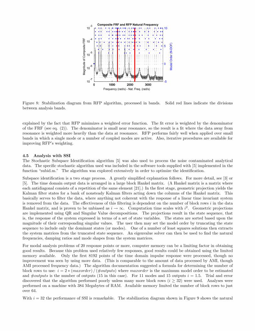
Despite the implementation of orthogonal polynomials, the global RFP solution became ill conditioned for asimultaneous fit of more than 9 or 10 modes. Consequently, it was decided to break the frequency range of interestinto at least three bands and fit each band individually. The analysis presented here used the following bands: ([0 to1300], [1300 to 2250], and [2250 to 3800] rad/s) Even then, RFP would just barely converge on the modes of interestbefore numerical ill-conditioning occurred. Figure 8 shows the stabilization diagrams for each band, concatenatedonto a single figure, with solid (red) vertical lines indicating the divisions between bands. The composite FRF issuperimposed.

A number of spurious modes are identified at the beginning and end of the analysis bands. These are especiallytroublesome because they are stable with model order, so they are hard to tell from true system modes. A singlemode is identified in the vicinity of close modes 8-9. Eigenvalues for modes 10 and 11 do not stabilize well enough forthese to be detected with any confidence. Even the most accurate eigenvalues found on the stabilization diagram weremuch less accurate than those found by AMI or SSI. The poor performance of the RFP algorithm is probably best

0 1000 2000 300010

-7

10-6

10-5

10-4

10-3 Composite FRF and RFP Natural Frequency

Mag

nitu

de o

f Com

posi

te F

RF

0 1000 2000 3000-5

0

5

10

Frequency (rad/s) - Nat. Freq. (rad/s)

Mod

el O

rder

(N-D

OF)

Figure 8: Stabilization diagram from RFP algorithm, processed in bands. Solid red lines indicate the divisionsbetween analysis bands.

explained by the fact that RFP minimizes a weighted error function. The fit error is weighted by the denominatorof the FRF (see eq. (2)). The denominator is small near resonance, so the result is a fit where the data away fromresonance is weighted more heavily than the data at resonance. RFP performs fairly well when applied over smallbands in which a single mode or a number of coupled modes are active. Also, iterative procedures are available forimproving RFP’s weighting.

4.5 Analysis with SSIThe Stochastic Subspace Identification algorithm [5] was also used to process the noise contaminated analyticaldata. The specific stochastic algorithm used was included in the software tools supplied with [5] implemented in thefunction “subid.m.” The algorithm was explored extensively in order to optimize the identification.

Subspace identification is a two stage process. A greatly simplified explanation follows. For more detail, see [3] or[5]. The time domain output data is arranged in a large block Hankel matrix. (A Hankel matrix is a matrix whereeach antidiagonal consists of a repetition of the same element [21].) In the first stage, geometric projection yields theKalman filter states for a bank of nonsteady Kalman filters acting down the columns of the Hankel matrix. Thisbasically serves to filter the data, where anything not coherent with the response of a linear time invariant systemis removed from the data. The effectiveness of this filtering is dependent on the number of block rows i in the dataHankel matrix, and is proven to be unbiased as i → ∞. Computation time scales with i2. Geometric projectionsare implemented using QR and Singular Value decompositions. The projections result in the state sequence, thatis, the response of the system expressed in terms of a set of state variables. The states are sorted based upon themagnitude of their corresponding singular values. The user then may set the model order by truncating the statesequence to include only the dominant states (or modes). One of a number of least squares solutions then extractsthe system matrices from the truncated state sequence. An eigenvalue solver can then be used to find the naturalfrequencies, damping ratios and mode shapes from the system matrices.

For modal analysis problems of 20 response points or more, computer memory can be a limiting factor in obtaininggood results. Because this problem used relatively few responses, good results could be obtained using the limitedmemory available. Only the first 8192 points of the time domain impulse response were processed, though noimprovement was seen by using more data. (This is comparable to the amount of data processed by AMI, thoughAMI processed frequency data.) The algorithm documentation suggested a formula for determining the number ofblock rows to use: i = 2 ∗ (maxorder) / (#outputs) where maxorder is the maximum model order to be estimatedand #outputs is the number of outputs (15 in this case). For 11 modes and 15 outputs i = 1.5. Trial and errordiscovered that the algorithm performed poorly unless many more block rows (i ≥ 32) were used. Analyses wereperformed on a machine with 384 Megabytes of RAM. Available memory limited the number of block rows to justover 64.

With i = 32 the performance of SSI is remarkable. The stabilization diagram shown in Figure 9 shows the natural

0 1000 2000 300010

-7

10-6

10-5

10-4

10-3 Composite FRF and SSI Natural Frequency

Mag

nitu

de o

f Com

posi

te F

RF

-20

-10

0

10

20

30

40

50

Frequency (rad/s) - Nat. Freq. (rad/s)

SSI M

odel

Ord

er (N

-DO

F)

Figure 9: Stabilization Diagram for SSI algorithm with 32 Block Rows

SIMO-AMI(Global AMI)

SSI (i = 32)N = 21 modes

Re Im*1000 Re Im*10000.01% 0.25% 4.1% 16.3%0.01% -0.01% 0.9% 0.8%-0.07% 0.08% 1.3% 2.0%0.04% 0.01% -2.6% -1.2%0.02% 0.16% 0.4% 0.3%0.03% -0.03% -1.2% 0.5%-0.35% -0.69% -2.4% -0.4%missed missed -11.4% 89.0%8.04% 26.43% -0.3% 45.1%4.10% 3.81% -1.5% 4.7%26.86% -15.94% 4.5% 6.2%

Table 3: Errors in Eigenvalues, SIMO-AMI and SSI

frequencies identified for model orders ranging from 10 to 50. The composite FRF is overlaid.

Only a small number of computational modes are identified in the frequency range of interest, though the true modesare easily discernible. All modes are identified, including the highly localized, weakly excited mode 8. The highquality of the results is not surprising. The data is contaminated only by the addition of white noise, which excludesmore troublesome errors, such as leakage, anti-alias filtering [4], nonlinearity, etc... SSI is based upon a model thatincludes zero-mean, random white noise, and it is proven to be convergent as the dimensions of the data Hankelmatrix approach infinity. Note also that all modes are not identified for model orders below 20, though only 11modes are present in the band of interest. Recall that 21 modes were used in constructing the analytical impulseresponse. The time domain data processed by SSI was not filtered to limit the effect of modes outside of the bandof interest. In a real problem, the true model order is infinite, and anti-aliasing filters or digital filters may be usedto reduce the effect of modes outside the frequency range of interest. In such a case, SSI would need to identify allpoles of the digital filter before absolute convergence could be obtained as in Figure 9, so this quality of results isnot likely to be possible for real problems.

Table 3 shows the error in the real and imaginary parts of the eigenvalues found by both SIMO-AMI and SSI.(Errors in the natural frequency and damping ratio are comparable to the errors in the imaginary and real partsrespectively.) Both algorithms are quite accurate for the first 7 modes, where the FRFs are clean, with the errors forSIMO-AMI being 1-2 orders of magnitude smaller than SSI. SSI identifies mode 8, and more accurately identifies thereal parts of the 9th and 10th eigenvalues, and the 11th eigenvalue. When compared to the peak picking method,SSI’s eigenvalues are order of magnitude more accurate on average, though the errors for many of the specific modesare comparable between the two methods.

-0.06 -0.04 -0.02 0 0.02 0.0410

15

20

25

30

35

40

45

50

Error-Imag Part (%)

Mod

el O

rder

Error in Imaginary Part of Eigenvalues versus Model Order

M1M2M3M4M5M6M7M8M9M10M11

M9

M11

M8

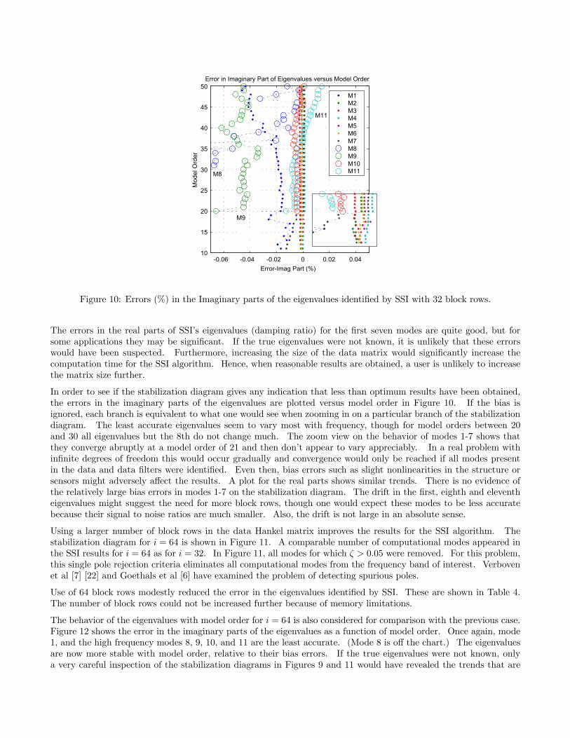
Figure 10: Errors (%) in the Imaginary parts of the eigenvalues identified by SSI with 32 block rows.

The errors in the real parts of SSI’s eigenvalues (damping ratio) for the first seven modes are quite good, but forsome applications they may be significant. If the true eigenvalues were not known, it is unlikely that these errorswould have been suspected. Furthermore, increasing the size of the data matrix would significantly increase thecomputation time for the SSI algorithm. Hence, when reasonable results are obtained, a user is unlikely to increasethe matrix size further.

In order to see if the stabilization diagram gives any indication that less than optimum results have been obtained,the errors in the imaginary parts of the eigenvalues are plotted versus model order in Figure 10. If the bias isignored, each branch is equivalent to what one would see when zooming in on a particular branch of the stabilizationdiagram. The least accurate eigenvalues seem to vary most with frequency, though for model orders between 20and 30 all eigenvalues but the 8th do not change much. The zoom view on the behavior of modes 1-7 shows thatthey converge abruptly at a model order of 21 and then don’t appear to vary appreciably. In a real problem withinfinite degrees of freedom this would occur gradually and convergence would only be reached if all modes presentin the data and data filters were identified. Even then, bias errors such as slight nonlinearities in the structure orsensors might adversely affect the results. A plot for the real parts shows similar trends. There is no evidence ofthe relatively large bias errors in modes 1-7 on the stabilization diagram. The drift in the first, eighth and eleventheigenvalues might suggest the need for more block rows, though one would expect these modes to be less accuratebecause their signal to noise ratios are much smaller. Also, the drift is not large in an absolute sense.

Using a larger number of block rows in the data Hankel matrix improves the results for the SSI algorithm. Thestabilization diagram for i = 64 is shown in Figure 11. A comparable number of computational modes appeared inthe SSI results for i = 64 as for i = 32. In Figure 11, all modes for which ζ > 0.05 were removed. For this problem,this single pole rejection criteria eliminates all computational modes from the frequency band of interest. Verbovenet al [7] [22] and Goethals et al [6] have examined the problem of detecting spurious poles.

Use of 64 block rows modestly reduced the error in the eigenvalues identified by SSI. These are shown in Table 4.The number of block rows could not be increased further because of memory limitations.

The behavior of the eigenvalues with model order for i = 64 is also considered for comparison with the previous case.Figure 12 shows the error in the imaginary parts of the eigenvalues as a function of model order. Once again, mode1, and the high frequency modes 8, 9, 10, and 11 are the least accurate. (Mode 8 is off the chart.) The eigenvaluesare now more stable with model order, relative to their bias errors. If the true eigenvalues were not known, onlya very careful inspection of the stabilization diagrams in Figures 9 and 11 would have revealed the trends that are

0 1000 2000 300010

-7

10-6

10-5

10-4

10-3 Composite FRF and SSI Natural Frequency

Mag

nitu

de o

f Com

posi

te F

RF

-20

-10

0

10

20

30

40

50

Frequency (rad/s) - Nat. Freq. (rad/s)

SSI M

odel

Ord

er (N

-DO

F)

Figure 11: Stabilization Diagram for SSI algorithm with 64 Block Rows. (Modes with ζ > 0.05 removed.)

SIMO-AMI(Global AMI)

SSI (i = 64)N = 21 modes

Re Im*1000 Re Im*10000.01% 0.25% -0.24% 5.79%0.01% -0.01% -3.27% -0.71%-0.07% 0.08% 0.23% 0.002%0.04% 0.01% -1.51% -0.36%0.02% 0.16% -1.07% -0.55%0.03% -0.03% 1.96% 0.35%-0.35% -0.69% 1.59% 0.34%missed missed 13.16% 111.48%8.04% 26.43% -0.14% -3.93%4.10% 3.81% 0.92% 7.03%26.86% -15.94% 10.22% 16.45%

Table 4: Errors in Eigenvalues, AMI-SIMO and SSI

evident in Figures 10 and 12.

Figures 10 and 12 indicate that scatter in the eigenvalues with model order might reveal when less than ideal resultshave been obtained, though this does not give a good indication of the absolute error in the eigenvalues. The usualpractice of creating a single stabilization diagram for a given number of block rows in the data Hankel matrix leadsto a false sense of security when it comes to the absolute accuracy of the estimates. A better practice might be tovary both model order and the number of block rows, though this would increase the computation time greatly.

The average of the absolute values of the errors for eigenvalues 1-7 and 9-11 for each method are presented in Table 5.Doubling the number of block rows used by the SSI algorithm has cut the errors in the imaginary parts approximatelyin half. For modes 1-7, SSI gives estimates of both real and imaginary parts that are an order of magnitude moreaccurate than the peak-picking method. AMI gives eigenvalue estimates that are two orders of magnitude moreaccurate than the peak-picking method. For modes 9-11 the trends are different. All methods show errors of aboutthe same order of magnitude as the peak picking method.

5 Computational Effort

For the test problem above AMI was the fastest algorithm. All computations were performed on a machine withan AMD-K7 processor and 384 Megabytes of RAM, using Windows 2000 and Matlab 6.1. AMI required less thanone minute of computation time in mode isolation and refinement to converge on accurate modal parameters. Little

-0.02 -0.015 -0.01 -0.005 0 0.005 0.0110

15

20

25

30

35

40

45

50

Error-Imag Part (%)

Mod

el O

rder

Error in Imaginary Part of Eigenvalues versus Model Order

M1M2M3M4M5M6M7M8M9M10M11

Figure 12: Errors (%) in the Imaginary parts of the eigenvalues identified by SSI with 64 block rows.

Average % Error in Real Parts

ModesPeakPick

SIMOAMI

SSI(i=32)

SSI(i=64)

1-7 9.7 % 0.1 % 1.8 % 1.4 %9-11 11.0 % 13.0 % 2.1 % 3.8 %

Average % Error in Imaginary Parts * 1000

ModesPeakPick

SIMOAMI

SSI(i=32)

SSI(i=64)

1-7 38.5 % 0.2 % 3.1 % 1.2 %9-11 25.3 % 15.4 % 18.6 % 9.1 %

Table 5: Average Percent Errors in Eigenvalues

computation was required during the subtraction stage, though the current version required user interaction to decidewhen to stop looking for modes.

The RFP algorithm used here was not optimized for Matlab as well as either AMI or SSI. The Matlab implementationof RFP took approximately ten minutes to process the data, though an optimized implementation may have beenfaster.

SSI was the most computationally intense algorithm. The QR and singular value decompositions took up the bulkof the computation time. For i = 32, 2.6 minutes of computation time were required to perform the decompositionsand find the system eigenvalues for model orders ranging from 10 to 50. For i = 64, 12.6 minutes of computation timewere required. While the differences between AMI and SSI in computation time are significant, memory requirementswere found to be the limiting factor in analyses with the SSI algorithm. Because only a limited number of responsepoints was used, good results were obtainable with the SSI algorithm within the constraint of physical memory. AMIused orders of magnitude less memory than SSI or the rational fraction polynomial method, so it could have reliablyfit many more response points No and frequencies L than used in this problem.

6 Conclusion

A simple, computationally efficient, global single—input-multi-output SDOF fitting algorithm has been presented andimplemented as a part of the Algorithm of Mode Isolation. (AMI) The resulting SIMO-AMI algorithm was found

to give more accurate results than a SISO-AMI algorithm for the test structure’s dominant modes. For the weaklyexcited modes, the SISO algorithm sometimes gave more accurate results. The SIMO algorithm missed one weaklyexcited mode because it’s response fell below the noise in the composite FRF. This reveals that, although modesare global properties of a structure, when measurement noise is significant, localized modes might be processed mostaccurately if the data that is fit pertains only to the degrees of freedom in which these modes are active. One benefitof the global algorithm is a great reduction in user interaction when compared to the SISO AMI algorithm.

The SIMO-AMI algorithm was found to give much more accurate results than the Rational Fraction Polynomial(RFP) algorithm for noise contaminated analytical data. This comparison is significant because the RFP algorithmis similar to AMI in mathematical form, though RFP attempts to identify all modes simultaneously.

The SSI algorithm identified the weakly excited mode 8, which was missed by SIMO-AMI, though the computationtime for the SSI algorithm was longer. The results demonstrated the importance of considering both model orderand the number of block Hankel rows used in the SSI fitting process. A stabilization diagram for a single numberof block rows may give a false sense of security as to the accuracy of the modal parameters identified.

When compared to the peak picking method, SSI and AMI respectively estimated the eigenvalues of modes 1-7 withone and two orders or magnitude more accuracy. For modes 9-11 the improvements over the peak-picking methodwere not as drastic.

The comparison of AMI and SSI should not necessarily be one of competition, as the best features of each algorithmcould be incorporated into a single algorithm if desired. For example, to improve it’s performance in the presenceof noise, AMI could be used to process the FFT of the state sequences found in the first stage of stochastic subspaceidentification. Conversely, the accuracy of the eigenvalues found by SSI could be improved by using SSI’s eigenvaluesas a starting point for the mode isolation and refinement stage of AMI. Perhaps the most notable contribution ofAMI is that it provides a different way of looking at the problem of modal identification, in which the importance ofeach mode to the experimental fit is clearly visible.

ACKNOWLEDGEMENT OF SUPPORT

This material is based on work supported under a National Science Foundation Graduate Research Fellowship.

References

[1] R. J. Allemang, Vibrations Course Notes. Cincinnati: http://www.sdrl.uc.edu/, 1999.[2] R. J. Allemang and D. L. Brown, “A unified matrix polynomial approach to modal identification,” Journal of Sound and

Vibration, vol. 211, no. 3, pp. 301—322, 1998.[3] K. D. Cock, B. Peeters, A. Vecchio, B. D. Moor, and H. V. D. Auweraer, “Subspace system identification for mechanical

engineering,” Proceedings of ISMA2002 - International Conference on Noise and Vibration Engineering, vol. III, (Leuven,Belgium), pp. 1333—1352, 2002.

[4] S. W. Doebling, K. F. Alvin, and L. D. Peterson, “Limitations of state-space system identification algorithms forstructures with high modal density,” 12th International Modal Analysis Conference (IMAC-12), (Honolulu, Hawaii),pp. 633—640, 1994.

[5] P. Van Overschee and B. De Moor, Subspace Identification for Linear Systems: Theory-Implementation-Applications.Boston: Kluwer Academic Publishers, 1996.

[6] I. Goethals and B. D. Moor, “Model reduction and energy analysis as a tool to detect spurious modes,” Proceedings ofISMA2002 - International Conference on Noise and Vibration Engineering, vol. III, (Leuven, Belgium), pp. 1307—1314,2002.

[7] P. Verboven, E. Parloo, P. Guillame, and M. V. Overmeire, “Autonomous modal parameter estimation based on astatistical frequency domain maximum likelihood approach,” 19th International Modal Analysis Conference (IMAC-19),(Kissimmee, Florida), pp. 1511—1517, 2001.

[8] H. V. D. Auweraer, W. Leurs, P. Mas, and L. Hermans, “Modal parameter estimation from inconsistent data sets,” 18thInternational Modal Analysis Conference (IMAC-18), (San Antonio, Texas), pp. 763—771, 2000.

[9] M. V. Drexel and J. H. Ginsberg, “Mode isolation: A new algorithm for modal parameter identification,” Journal of theAcoustical Society of America (JASA), vol. 110, no. 3, pp. 1371—1378, 2001.

[10] M. S. Allen and J. H. Ginsberg, “A linear least-squares version of the algorithm of mode isolation,” Submitted, 2004.[11] Y.-D. Joh and C.-W. Lee, “Excitation methods and modal parameter identification in complex modal testing of rotating

machinery,” International Journal of Analytical and Experimental Modal Analysis, vol. 8, no. 3, pp. 179—203, 1993.

[12] W. F. Pratt, M. S. Allen, and S. D. Sommerfeldt, “Testing and characterization of wavy composites,” in 46th InternationalSAMPE Symposium and Exhibition 2001 a Materials and Processes Odyssey, vol. 46 I, (Long Beach, CA), pp. 216—229,2001.

[13] J. H. Ginsberg, M. S. Allen, A. Ferri, and C. Moloney, “A general linear least squares sdof algorithm for identifyingeigenvalues and residues,” 21st International Modal Analysis Conference (IMAC-21), (Orlando, Florida), 2003.

[14] M. V. Drexel and J. H. Ginsberg, “Modal parameter identification using state space mode isolation,” 19th InternationalModal Analysis Conference (IMAC-19), (Orlando, FL), 2001.

[15] M. V. Drexel, J. H. Ginsberg, and B. R. Zaki, “State space implementation of the algorithm of mode isolation,” Journalof Vibration and Acoustics, vol. 125, pp. 205-213, 2003.

[16] J. H. Ginsberg, B. R. Zaki, and M. V. Drexel, “Application of the mode isolation algorithm to the identification of acomplex structure,” 20th International Modal Analysis Conference (IMAC-20), (Los Angeles, CA), pp. 794—801, 2002.

[17] J. H. Ginsberg and M. S. Allen, “Recent improvements of the algorithm of mode isolation,” Proceedings of IMECE’03,ASME International Mechanical Engineering Congress and Exposition, NCA, (Washington, DC), 2003.

[18] J. H. Ginsberg, Mechanical and Structural Vibrations. New York: John Wiley and Sons, 2001.[19] D. Formenti and M. Richardson, “Parameter estimation from frequency response measurements using rational fraction

polynomials (twenty years of progress),” 20th International Modal Analysis Conference (IMAC-20), (Los Angeles, CA),pp. 373—382, 2002.

[20] S. Maia, J. M. M. Silva, J. He, N. A. Lieven, R. M. Lin, G. W. Skingle, W. M. To, and A. P. V. Urgueira, Theoreticaland Experimental Modal Analysis. Taunto, Somerset, England: Research Studies Press Ltd., 1997.

[21] B. Peeters and G. D. Roeck, “Reference based stochastic subspace identification for output-only modal analysis,”Mechanical Systems and Signal Processing, vol. 13, no. 6, pp. 855—878, 1999.

[22] P. Verboven, P. Guillame, E. Parloo, and M. V. Overmeire, “Autonomous structural health monitoring—part 1:modalparameter estimation and tracking,” Mechanical Systems and Signal Processing, vol. 16, no. 4, pp. 637—657, 2002.