Signals in Robot Control: Two Primary Approachesgrupen/603/slides/... · v = fy z u = z fx pinhole...

Signals in Robot Control:Two Primary Approaches

I. Percept Inversion

Stimulus = f (World) World = f−1(S)

m −1m

• geometric reconstruction provides a representation forplanning and deliberation

• frame problem - completeness issues

• the functions, f (), are only partially known, and aregenerally difficult to invert

• time spent “perceiving” often renders world modelsobsolete

1 Copyright c©2014 Roderic Grupen

Signals in Robot Control:Two Primary Approaches

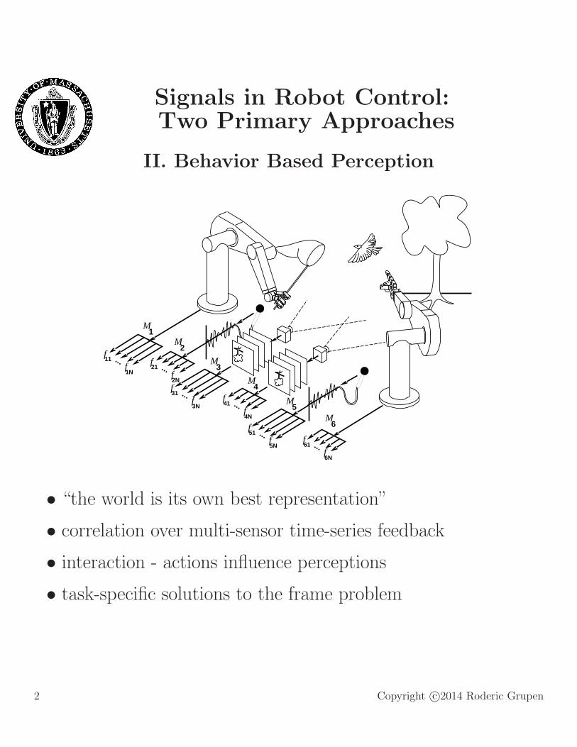
II. Behavior Based Perception

2M

M 6

M 5

M 4

M 3

M 1

...f61

f6N

...f

f51

5N

...f

f41

4N

...f

f31

3N

...f

f21

2N

...f

f11

1N

• “the world is its own best representation”

• correlation over multi-sensor time-series feedback

• interaction - actions influence perceptions

• task-specific solutions to the frame problem


Vision - Light and Matter

• Energy from a light source is radiated uniformly over 4π stera-dians → 1/R2 energy distribution from a point source

• the sun delivers about 1200Watts/m2 at noon on the equator

• at optical interfaces

– transmittion (refraction)

– reflection -diffuse or specular depending on surface prop-erties and wavelength.

– absorption - heat

– heat - black body radiation

• each encounter changes the properties of light - spectral con-tent, intensity, and polarization

...light signals carry a tremendous amount of information...


Vision - Pinhole Camera Revisited

v =fyz

zu =fx

pinholeaperture

planeimage

planeimage

pinholeaperture

focallength

focallength

v

z

u

y

xu

v

zy

x

• 5th century BC - Chinese philosopher Mo-Ti created an in-verted image by passing light through a pinhole into a darkened“collecting place.”

• ca. 350 BC - Aristotle viewed the eclipsing sun projected onthe ground through the holes in a sieve

• 10th century - Arabian scholar Alhazen of Basra created aportable solar observatory

• 15th - notebooks of Leonardo Da Vinci

• 17th century - Johannes Kepler - “camera obscura” (Latin for“room” and “dark,” respectively)


Vision - Pinhole Camera Revisited

v =fyz

zu =fx

pinholeaperture

planeimage

planeimage

pinholeaperture

focallength

focallength

v

z

u

y

xu

v

zy

x

• (1558) Giovanni Battista Della Porta “Magiae Naturalis” rec-ommended the camera obscura as a drawing aid for artists...

• 18th century artists used the camera obscura - Jan Vermeer,Canaletto, Guardi, and Paul Sandby

• 19th century - a sheet of light sensitive paper transforms thecamera obscura into the modern photographic camera.

What’s wrong with the pinhole camera?


Optics and Image Acquisition

optics

imageplane

source

...the radiant intensity function is projected onto a 2D im-age plane, sampled spatially, and digitized 30 times eachsecond...


Optics and Refraction - Gathering Light

Snell’s Law

incident

transmitted

reflected

Index of Refraction — theratio of the speed of light in avacuum to that in the optical ma-terial.

n =c

v=

√

ǫµ

ǫ0µ0

where

µ − magnetic permeability, and

ǫ − electric permittivity.

sin(θincident)

sin(θtransmitted)=

nt

ni,


Optics - Gaussian Lens Formula

Biconvex Thin Lens

1

S1+

1

S2=

1

f

f

2SS1

f


The Eye

(a) (b) (c) (d) (e)

cornea

iris

retinalens

pupil

suspensory ligaments

ciliarymuscle

aqueous humorvitreous

humor

visualaxis

blindspot

fovea

nasaltemple retina

80O

60O

40O

20O20

O

40O

60O

80O

opticnerve

(f)

superior oblique

superior rectus

inferiorrectus

inferioroblique

lateralrectus

levatorpalpebraesuperioris

superior oblique

superior rectus

medialrectus

inferiorrectus

inferioroblique

lateralrectus

superior rectus

inferioroblique

inferiorrectus

medialrectus

superior oblique

lateralrectus


Natural Variation

bees, fish, butterflies, birds and reptiles - capable of see-ing color—most mammals do not.

Herbivores - Side facing (monocular) vision systems yield al-most wrap around field of view.

Carnivores - forward facing (stereo) system provides precisiondepth and a narrower field of view (< 180 degrees)

Cheetah - wide, eccentric foveal region spanning horizontal bandfor locating prey against the horizon

Chamelion - turret eyes capable of both side- and forward-lookingconfigurations

Nocturnal - reflective back surface of retina - small birds sacrificemuscles for size. The largest eye belongs to the giant squid—upto 15 inches in diameter.

Fishing - fishing birds use polarizing lens

Rattlesnake - eyes oriented to side, forward-looking stereo pitorgans (no lens).


Where is the Information?

2M

M 6

M 5

M 4

M 3

M 1

...f61

f6N

...f

f51

5N

...f

f41

4N

...f

f31

3N

...f

f21

2N

...f

f11

1N

Information (the opposite of noise) resides in signalsthat exhibit reliable spatiotemporal structure

andyou can create spurious artifacts on signals

everytime you “touch” them...


Sampling - Spectral Propertiesof the Signal

Dirac delta operator:

δ(x− ξ) =

{

∞ x = ξ0 otherwise

This function has the following properties:

ǫ∫

−ǫ

δ(x)dx = 1 for ǫ > 0

∞∫

−∞

F (ξ)δ(x− ξ)dξ = F (x) Sifting Property


Sampling - Spectral Propertiesof the Signal

Fourier Transform

F [f (x)] = F (u) =

∞∫

−∞

f (x)exp{−i(2π(ux)}dx

where u is the spatial frequency (in cycles/meter), so that whenx is specified in meters, (2πux) is in radians, and i =

√−1.

F−1[F (u)] = f (x) =

∞∫

−∞

F (u)exp{i(2π(ux))}du


Fourier Transform Pairs

F (ω) = F(f(x)) =

∫ ∞

−∞f(x)e−iωxdx ω(rad/pixel) = 2πu(cycles/pixel)

Name f(x) F (ω)

rectangular function rect(x) = 1 − 12 < x < 1

2 sinc(ω/2π) = sin(ω/2)ω/2

triangular function tri(x) = 2(x+ 12) − 1

2 < x < 0 sinc2(ω/2π)1− 2(x) 0 < x < 1

2

Gaussian e−α|x| 2α/(α2 + ω2)

e−px2 1√2pe−ω2/4p

unit impulse δ(x) 1

comb function∑

n δ(x− nx0)1x0

∑

n δ(ω2π − n

x0

)


Example: Human Voice

the open-closed resonance cavity—a constant diameter tube openat one end that radiates sound pressure into an infinitely largerenvironment

the open end of the cavity reflects an inverted pressure wave

F = 1/4(c/L) Hz1

F = 3/4(c/L) Hz2

F = 5/4(c/L) Hz3

f(t) = sin(2 F t)2

f(t) = sin(2 F t)3

st1 formantnd

2 formant rd3 formant

f(t) = sin(2 F t)1

ωn = (2n− 1)(c/4L)

several resonance modes (formants) exist simultaneously


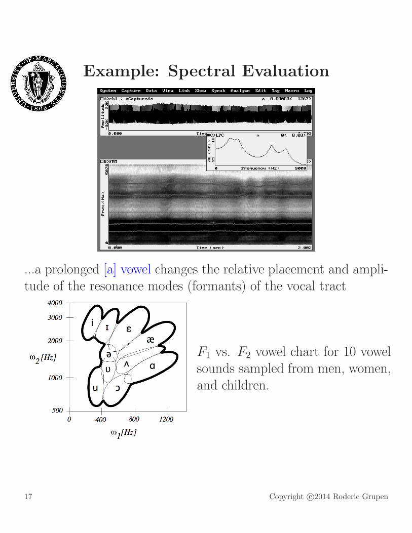
Example: Spectral Evaluation

“...the rainbow passage...”

A screen capture from an analysis by the Computerized SpeechLab (courtesy Dr. M. Andrianopoulos): frequency content versustime; sound pressure level as a function of frequency, and ampli-tude versus time for a vocalization.


Example: Spectral Evaluation

...a prolonged [a] vowel changes the relative placement and ampli-tude of the resonance modes (formants) of the vocal tract

F1 vs. F2 vowel chart for 10 vowelsounds sampled from men, women,and children.


Shift Theorem

F [f (x)] =

∞∫

−∞

f (x)exp{−i(2πux)}dx, then

F [f (x− a)] =

∞∫

−∞

f (x− a)exp{−i(2πux)}dx, then

=

∞∫

−∞

f (x′)exp{−i(2πu(x′ + a))}dx′, and

= exp{−i(2πua)}∞∫

−∞

f (x′)exp{−i(2πux′)}dx′,

so that

F [f (x− a)] = exp{−i(2πua)}F(f (x))


Convolution Theorem

f (x) ∗ g(x) = h(x) =

∫ ∞

−∞f (α)g(x− α)dα

where α an integration variable.

F [f (x) ∗ g(x)] = F [h(x)]

= F[∫

α

f (α)g(x− α)dα

]

=

∫

x

[∫

α

f (α)g(x− α)dα

]

exp{−i2πux}dx

=

∫

α

f (α)

[∫

x

g(x− α)exp{−i(2πux)}dx]

dα

and by the Shift theorem,

=

∫

α

f (α)exp{−i(2πuα)}dα∫

x

g(x)exp{−i(2πux)}dx,

and therefore,F [f (x) ∗ g(x)] = F (u)G(u)

spatial/temporal convolution ↔ frequency domain multiplication


Sampling Theorem - Aliasing

A continuous spatial function, f (x)is sampled by computing the prod-uct of f (x) and g(x), an infinite se-quence of Dirac delta operators.

h(x) = f (x)∑

n

δ(x− nx0)

=∑

n

f (nx0)δ(x− nx0)

By the convolution theorem, theproduct of these two spatial func-tions is the convolution of theirFourier transform pairs.

f(x)

g(x)

h(x)

x02 x04 x06x0−2x0−4x0−6

f (x)F−→ F (u)

∑

n

δ(x− nx0)F−→ 1

x0

∑

n

δ(u− n

x0) = G(u), and

H(u) = F (u) ∗G(u)


Sampling Theorem - Aliasing (cont.)

H(u) = F (u) ∗G(u)

We may write the function H(u) in terms of F (u):

H(u) = F (u)∗[

1

x0

∑

n

δ(u− n

x0)

]

=

∫ ∞

−∞F (α)G(u− α)dα

=

∫ ∞

−∞F (α)

[

1

x0

∑

n

δ(u− α− n

x0)dα

]

=1

x0

∫ ∞

−∞

∑

n

F (u− n

x0)δ(u− α− n

x0)dα

=1

x0

∑

n

F (u− n

x0)

∫ ∞

−∞δ(u− α− n

x0)dα

H(u) =1

x0

∑

n

F (u− n

x0)

the frequency spectrum of the sampled image contains of dupli-cates of the spectrum of the original image distributed at 1/x0frequency intervals.


Aliasing (cont.)

x01/ x02/x0−1/x0

−2/

x01/ x02/x0−1/x0

−2/

(a)

(b)

Η( )ω R( )H( )ω ω

R(u) is a frequency domainbandpass filter

R(u) = 1 if |u| < 1/(2x0),

0 otherwise

Aliasing: When replicated spectra interfere, the crosstalk intro-duces energy at relatively high frequencies changing the appear-ance of the reconstructed image.

The Sampling Theorem:

If the image contains no frequency components greater than

one half the sampling frequency, then the continuous image is

faithfully represented in the sampled image.


Early Processing - Convolution

f (x, y)∗g(x, y) = h(x, y) =

∫ ∞

−∞

∫ ∞

−∞f (u, v)g(x−u, y−v)dudv

or

f (x, y) ∗ g(x, y) = h(x, y) =

∞∑

−∞

∞∑

−∞f (u, v)g(x− u, y − v)

g(x,y)

h(x,y)

h(n,n)

f(3,3)

g(n,n)


Early Processing

...if you know what you’re looking for, convolution can be used asa means of approximating the correlation of a signal fragment toa reference template...

Rgt =∑

α

∑

β

t(α, β)g(x + α, y + β).

maxima in Rgt are minima in:

α∑

i=−α

β∑

j=−β

[g(x + i, y + j)− t(α, β)]2


Frei and Chen Templates

...patterns of responses can be more robust andmore informative than single operators...

1 1 11 1 11 1 1

f0

−1 −√2 −1

0 0 0

1√2 1

f1

−1 0 1

−√2 0

√2

−1 0 1

f2

0 −1√2

1 0 −1

−√2 1 0

f3

√2 −1 0

−1 0 1

0 1 −√2

f4

0 1 0−1 0 −10 1 0

f5

−1 0 10 0 01 0 −1

f6

1 −2 1−2 4 −21 −2 1

f7

−2 1 −21 4 1−2 1 −2

f8

Frobenius inner product A : B = trace(ABT ) = trace(ATB) ofany pair of Frei-Chen operators is zero

each operator captures an independent “shape” in 3× 3neighborhoods of the luminosity surface

the image is characterized as a vector of responses, h(x, y), where

hk = fk ∗ g, k ∈ [0, 8].


Frei and Chen Templates

hk = fk ∗ g

Edge Energy(x, y) =

2∑

k=1

h2k(x, y)

Total Energy(x, y) =

8∑

k=0

h2k(x, y)

define:

cos(θ) =

(

EE

TE

)1/2

gradientmagnitudethreshold

Frei−Chenthreshold

TotalEnergy

Edge Energy

TotalEnergy

Edge Energy

θ

1

1EE(x ,y )1

EE(x ,y )2 2

1EE(x ,y )1

EE(x ,y )2 2


Early Processing -Differential Geometry

Low Pass Filter

g(x)

h(x)

f(x)

*h = f g

1

x−1/2 +1/2

rect(x)sinc( ) =

ω2π (ω/2)

ω/2sin( )1

5 10 15 20 250−5−10−15−20−25ω

F

F−1


Early Processing -Gradient Operators

Intensity Gradients

∇g =dg

dxx +

dg

dyy

dg(x, y)

dx≈ g(x + 1, y)− g(x− 1, y)

2⇒ fx =

[

−1

2, 0,

1

2

]

1×3

dg(x, y)

dy≈ g(x, y + 1)− g(x, y − 1)

2⇒ fy =

−12012

3×1

|∇g| =

[

(

dg

dx

)2

+

(

dg

dy

)2]

12

=

φ = tan−1

(

dg/dy

dg/dx

)


Edge Operators

operator ∇1 ∇2

Roberts[

0 1−1 0

] [

1 00 −1

]

Prewit

−1 0 1−1 0 1−1 0 1

1 1 10 0 0

−1 −1 −1

Sobel

−1 0 1−2 0 2−1 0 1

1 2 10 0 0

−1 −2 −1


Early Processing - Edge Sharpening

Laplacian

∇2g =d2g

dx2+

d2g

dy2⇒ f =

0 −1 0−1 4 −10 −1 0

2

f(x)

f(x)

f(x)


Summary: Signals, Sampling, and Features

• optics and the evolution of the eye

• spectral analysis and the sampling theorem

• convolution - feature-based early processing, the spectral in-terpretation of convolution operators

Today: Deep Structure and Information

• differential structure - edge sharpening algorithm

• the Canny edge operator and Gaussian operators

• multi-scale feature detectors

– edge sharpening revisited

– gauge coordinates and scale space

– oriented edges, ridges, corners, blobs


Deep Structure

...consider a multivariate signal f (x1, . . . , xn) in the vicinity of(x01, . . . , x

0n), represented by its Taylor series expansion:

f (x1, . . . , xn) = f (x01, . . . , x0n)+

∞∑

m=1

∑

k1,...,kn∑

j kj=m

∂mf (x01, . . . , x0n)

∂xk11 · · · ∂xknn

[

(x1 − x01)k1

k1!· · · (xn − x0n)

kn

kn!

]

Definition (N-jet): spatial derivatives

∂mf (x01, . . . , x0n)

∂xk11 · · · ∂xknn, m ∈ [0, N ],

∑

j

kj = m.

characterize differential structure up to order N .


Scale Space and the N-jet

Image Processing

the N -jet of order 2 for function f (x, y) is the set(

f,∂f

∂x,∂f

∂y,∂2f

∂x2,

∂2f

∂x∂y,∂2f

∂y2

)

.

Topological structure in the luminance function (critical points,extremum, ridge points, corners, blobs) can be captured in termsof differential structure and form a basis for structural informationtheory.

Structures that are persistent across the scale dimension constitutethe “deep structure” of signals.

f (x, y, σ)

.

...how should N -jet operators be chosen?


Differential Convolution Operators

Suppose:

f (x) : image function

gσ(x) =1√2πσ

e−x2/2σ2 : Gaussian smoothing function

Then:

f ∗ g ⇒ bandlimited approximation of image f (x)

⇒ suppress noise prior to differentiationd

dt(f ∗ g) ⇒ edges in the image f (x)

Canny Edge Operator

d

dt(f ∗ g) = f ∗ d

dtg


Gaussian Operatorsin the Frequency Domain


Multi-Scale Feature Detectors

from before, edge sharpening:

∇2f (x, y) = 0, and

|∇f | > τ.

Oriented Edges

“steerable” filters - gauge coordinates

a local orthonormal coordinate frame (u, v) oriented with the v-axis parallel to the gradient direction at position (x, y).

by this definition, fv is always positive and the lateral first deriva-tive, fu, is zero.

fvv = 0, and

fvvv < 0.

• coarse scales suppress noise, fine scales localize more precisely,

• most sharp edge structures corresponding to object boundariesexist simultaneously at many scales.


Multi-Scale Oriented Edges

Edges reported at t=1.0, 16.0, and 256.0, respectively


Multi-Scale Feature Detectors

Oriented Ridges

gauge coordinates (p, q) - aligns the local principal curvature ofthe luminocity function such that off-diagonal terms in the imageHessian, fpq = fqp = 0.

A ridge is an extremum in the direction of the maximum principalcurvature, which we align with direction p:

fp = 0,

fpp < 0, and |fpp| ≥ |fqq|

dominant ridge structures can be found at all scales.


Multi-Scale Oriented Ridges

Ridges reported at t=1.0, 16.0, and 256.0, respectively


Intrinsic Scale

feature featuretype strength

edge√σ

21/4fv

ridge σ3

23/2(fpp − fqq)

2

corner σ4

4 fvfuu

blob σ2

2 ∇2f

search for scales at which feature strength is maximized


Intrinsic Scale - Corners, and Blobs


Signals in Robot Control: Two Primary Approachesgrupen/603/slides/... · v = fy z u = z fx pinhole...

Documents

Transcript of Signals in Robot Control: Two Primary Approachesgrupen/603/slides/... · v = fy z u = z fx pinhole...