Chapter 2

Signal and system norms

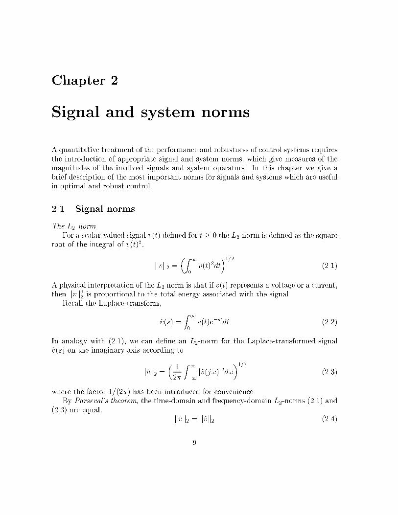
A quantitative treatment of the performance and robustness of control systems requires

the introduction of appropriate signal and system norms, which give measures of themagnitudes of the involved signals and system operators. In this chapter we give abrief description of the most important norms for signals and systems which are usefulin optimal and robust control.

2.1 Signal norms

The L2 norm

For a scalar-valued signal v(t) de�ned for t � 0 the L2-norm is de�ned as the squareroot of the integral of v(t)2,

kvk2 =

�Z1

0

v(t)2dt

�1=2(2.1)

A physical interpretation of the L2 norm is that if v(t) represents a voltage or a current,then kvk2

2is proportional to the total energy associated with the signal.

Recall the Laplace-transform,

v(s) =

Z1

0

v(t)e�stdt (2.2)

In analogy with (2.1), we can de�ne an L2-norm for the Laplace-transformed signalv(s) on the imaginary axis according to

kvk2 =

�1

2�

Z1

�1

jv(j!)j2d!

�1=2(2.3)

where the factor 1=(2�) has been introduced for convenience.

By Parseval's theorem, the time-domain and frequency-domain L2-norms (2.1) and(2.3) are equal,

kvk2 = kvk2 (2.4)

9

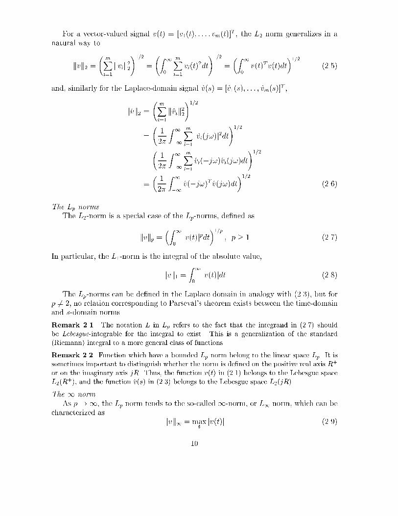
For a vector-valued signal v(t) = [v1(t); : : : ; vm(t)]T , the L2 norm generalizes in a

natural way to

kvk2 =

mXi=1

kvik2

2

!1=2=

Z1

0

mXi=1

vi(t)2dt

!1=2=

�Z1

0

v(t)Tv(t)dt

�1=2(2.5)

and, similarly for the Laplace-domain signal v(s) = [v1(s); : : : ; vm(s)]T ,

kvk2 =

mXi=1

kvik2

2

!1=2

=

1

2�

Z1

�1

mXi=1

jvi(j!)j2dt

!1=2

=

1

2�

Z1

�1

mXi=1

vi(�j!)vi(j!)dt

!1=2

=

�1

2�

Z1

�1

v(�j!)T v(j!)dt

�1=2(2.6)

The Lp norms

The L2-norm is a special case of the Lp-norms, de�ned as

kvkp =

�Z1

0

jv(t)jpdt

�1=p; p � 1 (2.7)

In particular, the L1-norm is the integral of the absolute value,

kvk1 =Z1

0

jv(t)jdt (2.8)

The Lp-norms can be de�ned in the Laplace domain in analogy with (2.3), but forp 6= 2, no relation corresponding to Parseval's theorem exists between the time-domainand s-domain norms.

Remark 2.1. The notation L in Lp refers to the fact that the integrand in (2.7) should

be Lebesgue-integrable for the integral to exist. This is a generalization of the standard

(Riemann) integral to a more general class of functions.

Remark 2.2. Function which have a bounded Lp norm belong to the linear space Lp. It is

sometimes important to distinguish whether the norm is de�ned on the positive real axis R+

or on the imaginary axis jR. Thus, the function v(t) in (2.1) belongs to the Lebesgue space

L2(R+), and the function v(s) in (2.3) belongs to the Lebesgue space L2(jR).

The 1-norm

As p!1, the Lp norm tends to the so-called1-norm, or L1norm, which can be

characterized askvk

1= max

tjv(t)j (2.9)

10

supposing that the maximum exists. However, there is in general no guarantee that

the maximum in (2.9) exists, and therefore the correct way is to de�ne the L1

normas the least upper bound (or supremum) of the absolute value,

kvk1= sup

tjv(t)j (2.10)

Example 2.1. The function

f(x) =

�x; if jxj < 1

0; if jxj � 1(2.11)

has no maximum, because for any x = x1, x1 = 1 � � say (where � > 0), one can select

another value x2, such that f(x2) > f(x1) (take for example x2 = 1 � �=2). Therefore, one

instead introduces the least upper bound or supremum de�ned as the least number M which

satis�es M � f(x) for all x, i.e.,

supxf(x) = minfM : f(x) �M; all xg (2.12)

For the function in (2.11), supx f(x) = 1. Notice that the minimum in (2.12) exists.

The greatest lower bound or in�mum is de�ned in an analogous way. The function in

(2.11) does not have a minimum, but its greatest lower bound is infx f(x) = �1.

Remark 2.3. A more correct way would be to write the L1-norm as

kvk1

= ess suptjv(t)j (2.13)

indicating that points of measure zero (i.e., isolated points) are excluded when taking the

supremum or maximum. However, the functions normally treated in this course are continu-

ous, and therefore we will use the de�nitions (2.9) or (2.10).

2.2 System norms

2.2.1 The H2 norm

For a stable SISO linear system with transfer function G(s), the H2-norm is de�ned inanalogy with (2.3) as

kGk2 =

�1

2�

Z1

�1

jG(j!)j2d!

�1=2(SISO) (2.14)

For a multivariable system with transfer function matrix G(s) = [gkl(s)], the de�nitiongeneralizes to

kGk2 =

Xkl

kgklk2

2

!1=2

=

1

2�

Z1

�1

Xkl

jgkl(j!)j2d!

!1=2

11

=

1

2�

Z1

�1

Xkl

gkl(�j!)gkl(j!)d!

!1=2

=

�1

2�

Z1

�1

tr[G(�j!)TG(j!)]d!

�1=2(2.15)

In the last equality, we have used the result (2.16) below.

Problem 2.1. Show that for n�m matrices A = [akl] and B = [bkl],

tr[ATB] =nX

k=1

mXl=1

aklbkl = a11b11 + � � �+ anmbnm (2.16)

Notice in particular that in the case A = B, equation (2.16) gives the sum of the squares of

the elements of a matrix,

tr[ATA] =nX

k=1

mXl=1

a2kl = a211 + � � �+ a2nm (2.17)

Remark 2.4 The notation H in H2 (instead of L) is due to the fact that the function spaces

which, in addition to having �nite Lp norms on the imaginary axis (cf. equation (2.3)), are

bounded and analytic functions in the right-half plane (i.e. with no poles in the RHP), are

called Hardy spaces Hp. Thus, stable transfer functions belong to these spaces, provided

the associated integral is �nite. The spaces are called after the British pure mathematician

G. H. Hardy (1877{1947).

State-space computation of the H2 norm

Rather than evaluating the integrals in (2.14) or (2.15) directly, the H2 norm of atransfer function is conveniently calculated in the time-domain. In particular, assumethat the stable transfer function G(s) has state-space representation

_x(t) = Ax(t) +Bv(t)

z(t) = Cx(t) (2.18)

so thatG(s) = C(sI � A)�1B (2.19)

Integrating (2.18) from 0 to t gives for z(t),

z(t) = CeAtx(0) +

Z t

0

H(t� �)v(�)d� (2.20)

where H(t� �) is the impulse response function de�ned as

H(�) =

�CeA�B; if � � 00; if � < 0

(2.21)

Problem 2.2. Verify (2.20).

12

It is straightforward to show that G(s) is simply the Laplace-transform of the

impulse response function H(�),

G(s) =

Z1

0

H(�)e�s�d� (2.22)

Problem 2.3. Verify (2.22).

From Parseval's theorem applied to H(t) and its Laplace transform G(s) it thenfollows that kG2k equals the corresponding time-domain norm of the impulse responsefunction H,

kGk2 = kHk2 (2.23)

where

kHk2 =

Z1

0

Xkl

hkl(t)2dt

!1=2=

�Z1

0

tr[H(t)TH(t)]dt

�1=2(2.24)

Notice that kHk2 is �nite if the system is stable, i.e., all eigenvalues of the matrix Ahave strictly negative real parts. By (2.23), we can evaluate the H2 norm in (2.15) bycomputing the time-domain norm in (2.24). From (2.21) and (2.24) we have

kGk22= kHk2

2= tr[C

Z1

0

eAtBBT eAT tdtCT ] (2.25)

De�ning the matrix

P =

Z1

0

eAtBBT eAT tdt (2.26)

equation (2.25) can be written

kHk22= tr[CPCT ] (2.27)

It turns out that the matrix P is the unique solution to the linear matrix equation

AP + PAT +BBT = 0 (2.28)

Equation (2.28) is known as a matrix Lyapunov equation, due to the fact that it isassociated with Lyapunov stability theory of linear systems.

The fact that P is the solution to (2.28) can be shown by observing that

d

dteAtBBT eA

T t = AeAtBBT eAT t + eAtBBT eA

T tAT (2.29)

and integrating both sides from 0 to 1. The left-hand side givesZ1

0

d

dteAtBBT eA

T tdt = eAtBBT eAT t���10= �BBT (2.30)

where the fact has been used that exp(At), due to stability, converges to zero as t!1.On the right-hand side of (2.29) the de�nition of P givesZ

1

0

[AeAtBBT eAT t + eAtBBT eA

T tAT ]dt = AP + PAT (2.31)

13

and thus (2.28) follows.

There are e�cient numerical methods for solving the linear matrix equation (2.28).In MATLABs control toolboxes (2.28) can be solved using the routine lyap.

Signal interpretations of the H2 norm

It is useful to interpret the H2 norm de�ned for a system transfer function in termsof the input and output signals of the system.

Consider the linear systemz(s) = G(s)v(s) (2.32)

Assuming a SISO system, suppose that the input has the transform

v(s) = 1 (2.33)

implying that it contains equal amounts of all frequencies (because v(j!) = 1). Thenthe output has the transform

z(s) = G(s) (2.34)

and according to (2.3), its L2 norm equals

kzk2 =

�1

2�

Z1

�1

jG(j!)j2d!

�1=2= kGk2 (2.35)

Hence kGk2 can be interpreted as an average system gain taken over all frequencies.The above result is generalized to the MIMO case by considering the e�ect of one

input at a time. Let the kth input have a constant Laplace transform equal to one,while the other inputs are zero. Then v(s) can be written as

v(s) = ek (2.36)

where ek denotes the kth unit vector,

ek = [0 � � �0 1 0 � � �0]T (2.37)

where the 1 is in the kth position. With this input, the output is Z(s) = G(s)ek andthe square of its L2 norm is given by

kzk22= kGekk

2

2

=1

2�

Z1

�1

eTkG(�j!)TG(j!)ekd!

=1

2�

Z1

�1

tr[G(�j!)ekeTkG(j!)

T ]d! (2.38)

where we have used the identity

tr[AB] = tr[ATBT ] (2.39)

14

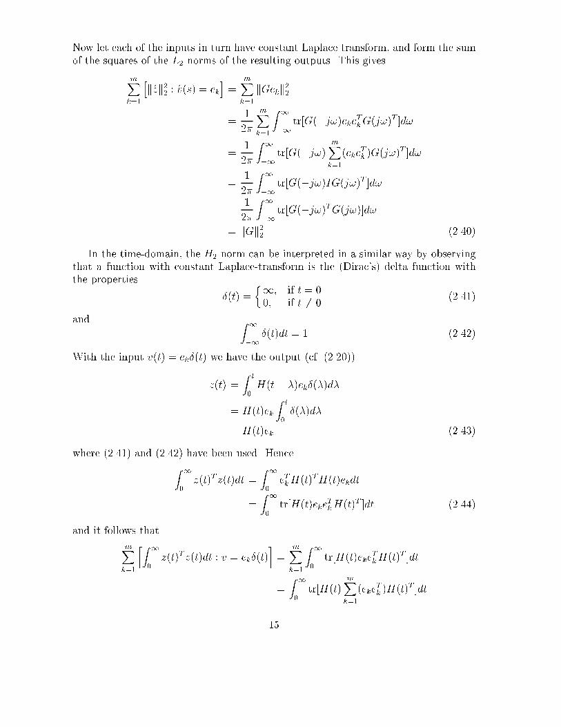
Now let each of the inputs in turn have constant Laplace transform, and form the sum

of the squares of the L2 norms of the resulting outputs. This gives

mXk=1

hkzk2

2: v(s) = ek

i=

mXk=1

kGekk2

2

=1

2�

mXk=1

Z1

�1

tr[G(�j!)ekeTkG(j!)

T ]d!

=1

2�

Z1

�1

tr[G(�j!)mXk=1

(ekeTk )G(j!)

T ]d!

=1

2�

Z1

�1

tr[G(�j!)IG(j!)T ]d!

=1

2�

Z1

�1

tr[G(�j!)TG(j!)]d!

= kGk22

(2.40)

In the time-domain, the H2 norm can be interpreted in a similar way by observingthat a function with constant Laplace-transform is the (Dirac's) delta function withthe properties

�(t) =

�1; if t = 00; if t 6= 0

(2.41)

and Z1

�1

�(t)dt = 1 (2.42)

With the input v(t) = ek�(t) we have the output (cf. (2.20))

z(t) =

Z t

0

H(t� �)ek�(�)d�

= H(t)ek

Z t

0

�(�)d�

= H(t)ek (2.43)

where (2.41) and (2.42) have been used. HenceZ1

0

z(t)T z(t)dt =

Z1

0

eTkH(t)TH(t)ekdt

=

Z1

0

tr[H(t)ekeTkH(t)T ]dt (2.44)

and it follows that

mXk=1

�Z1

0

z(t)T z(t)dt : v = ek�(t)

�=

mXk=1

Z1

0

tr[H(t)ekeTkH(t)T ]dt

=

Z1

0

tr[H(t)mXk=1

(ekeTk )H(t)T ]dt

15

=

Z 1

0

tr[H(t)IH(t)T ]dt

=

Z 1

0

tr[H(t)TH(t)]dt

= kHk22

(2.45)

It is also worth while to observe that the H2norm has a particularly nice interpre-

tation in a stochastic framework. Without going into details of the (rather di�cult)

theory of continuous-time stochastic systems, let us note that if the input v is a (vector-valued) white noise signal with unit covariance matrix, Rv = I, then the sum of thestationary variances of the outputs is given by the square of the H

2norm of the transfer

function, i.e.,

limtf!1

E[1

tf

Z tf

0

zT (t)z(t)dt] = kGk22

(2.46)

Recalling that white noise contains equal amounts of all frequencies, it is understood

that the characterization (2.46) is simply the stochastic counterpart of the characteri-zations in (2.40) and (2.45).

2.2.2 The H1 norm

In addition to the H2norm, which we have seen gives a characterization of the average

gain of a system, a perhaps more fundamental norm for systems is the H1 norm, whichprovides a measure of a worst-case system gain.

The H1 norm for SISO systemsConsider a stable SISO linear system with transfer function G(s). The H1 norm

is de�ned askGk1 = max

!jG(j!)j (SISO) (2.47)

or, in the event that the maximum may not exist, more correctly as

kGk1 = sup!jG(j!)j (SISO) (2.48)

See also Remark 2.3. Recalling that jG(j!)j is the factor by which the amplitude of asinusoidal input with angular frequency ! is magni�ed by the system, it is seen that theH1 norm is simply a measure of the largest factor by which any sinusoid is magni�edby the system.

A very useful interpretation of the H1 norm is obtained in terms of the e�ect of Gon the space of inputs with bounded L

2norms. (Notice that a sinusoidal signal does

not have bounded L2norm because the integral in (2.1) is unbounded.) Let v(t) be

a signal with Laplace-transform v(s) such that the L2norm given by (2.1) or (2.3) is

bounded. Then the system output z(s) = G(s)v(s) has L2norm given by (2.3) which

is bounded above by kGk1kvk2, because

kGvk2=

�1

2�

Z 1

�1jG(j!)v(j!)j2d!

�1=2

16

=

�1

2�

Z 1

�1jG(j!)j2jv(j!)j2d!

�1=2

� sup!jG(j!)j

�1

2�

Z 1

�1jv(j!)j2d!

�1=2

= kGk1kvk2 (2.49)

Hence

kGk1 �kGvk

2

kvk2

; all v 6= 0 (2.50)

In fact there exist signals v which come arbitrarily close to the upper bound in (2.49).

This can be understood by letting v be such that its Laplace-transform on the imaginaryaxis v(j!) is concentrated to a frequency range where jG(j!)j is arbitrarily close tokGk1, and with v(j!) equal to zero elsewhere. Then it follows that the H1 norm canbe characterized as

kGk1 = sup

(kGvk

2

kvk2

: v 6= 0

)(2.51)

Hence the H1 norm gives the maximum factor by which the system magni�es the L2

norm of any input. Therefore, kGk1 is also called the gain of the system. In operatortheory, an operator norm like that in (2.51) is called an induced norm. The H1 norm

is an operator norm which induced by the L2norm.

The H1 norm for MIMO systemsFor multivariable systems, the H1 norm is de�ned in an analogous way. Let's

�rst see how the de�nition in (2.47) could be extended to the multivariable case. TheSISO gain jG(j!)j at a given frequency should then be generalized to the multivariablecase. For an n�m transfer function matrix G(s), a natural way to achieve this is tointroduce the maximum gain of G(j!) at the frequency !. For this purpose, introduce

the Euclidean norm kvk of a complex-valued vector v = [v1; : : : ; vm]

T 2 Cm,

kvk =�jv1j2 + � � �+ jvmj

2

�1=2

(2.52)

The maximum gain of G at the frequency ! is then given by the quantity

kG(j!)k = maxv

(kG(j!)vk

kvk: v 6= 0; v 2 Cm

)

= maxvfkG(j!)vk : kvk = 1; v 2 Cmg (2.53)

In analogy with (2.47), or (2.48), the H1 norm of the transfer function matrix G(s) isde�ned as

kGk1 = sup!kG(j!)k (2.54)

where kG(j!)k is given by (2.53). It will be shown below that the matrix norm kG(j!)kis equal to the maximum singular value ��(G(j!)) of the matrix G(j!). Therefore the

H1 norm is often expressed as

kGk1 = sup!

��(G(j!)) (2.55)

17

In analogy with (2.48), (2.54) can be interpreted in terms of the e�ect that the

system G has on sinusoidal inputs. Let the input be a vector-valued sinusoidal givenby

v(t) = [a1sin(!t+ �

1); � � � ; am sin(!t+ �m)]

T (2.56)

The output z = Gv is then another vector-valued sinusoid with the same angularfrequency ! as the input, but with components whose magnitudes and phases are

transformed by the system,

z(t) = [c1sin(!t+ �

1); � � � ; cn sin(!t+ �n)]

T (2.57)

Expressing the magnitude of the sinusoidal vectors in analogy with the Euclidean norm,

kvk =�a21+ � � �+ a2m

�1=2

kzk =�c21+ � � �+ c2n

�1=2

(2.58)

it can be shown that (2.54) is equal to the quantity

kGk1 = sup!

maxfaig;f�ig

(kzk

kvk: z = Gv; v given by (2.56)

)(2.59)

Hence the H1 norm is the maximum factor by which the magnitude of any vector-valued sinusoidal input, as de�ned by (2.56), is magni�ed by the system. The proof of

(2.59) involves a bit of algebraic manipulations, and it is left as an exercise.A more important characterization of the H1 norm is in terms of the e�ect on

signals with bounded L2norms. Let v denote a signal with bounded L

2norm, and

with Laplace-transform v(s). Then the L2norm of the system output z(s) = G(s)v(s)

is bounded in analogy with (2.49). Using (2.6),

kGvk2=

�1

2�

Z 1

�1v(�j!)TG(�j!)TG(j!)v(j!)d!

�1=2

=

�1

2�

Z 1

�1kG(j!)v(j!)k2d!

�1=2

�

�1

2�

Z 1

�1[kG(j!)kkv(j!)k]2d!

�1=2

(cf. (2.53))

� sup!kG(j!)k

�1

2�

Z 1

�1kv(j!)k2d!

�1=2

= kGk1kvk2 (2.60)

Just as in the SISO case, the upper bound in (2.60) is tight. Suppose that the Laplace

transform v(s) is concentrated to a frequency range where kG(j!)k is arbitrary closeto kGk1, and with components such that kG(j!)v(j!)k=kv(j!)k is arbitrary close tokG(j!)k. Then it is understood that (2.51) holds for the multivariable case as well,and the H1 norm is the operator norm induced by the L

2norm, i.e.

kGk1 = sup

(kGvk

2

kvk2

: v 6= 0

)(2.61)

18

The de�nition of the H1 norm above has made use of the matrix norm de�ned in

(2.53). The characterization of this norm, and in particular its relation to the singularvalues of a matrix, is discussed in more detail in Section 2.2.3.

State-space computation of the H1 norm

The characterizations (2.51) and (2.61) provide a very useful method to evaluatethe H1 norm by state-space formulae. Let G(s) have the state-space representation

_x(t) = Ax(t) +Bv(t)

z(t) = Cx(t) +Dv(t) (2.62)

so thatG(s) = C(sI � A)�1B +D (2.63)

By Parseval's theorem, the H1 norm can be characterized in the time domain as

kGk1 = sup

(kzk

2

kvk2

: v 6= 0

)(2.64)

It follows that for any > 0, kGk1 < if and only if

J1(G; ) :=maxv

hkzk2

2� 2kvk2

2

i= max

v

Z 1

0

hzT (t)z(t)� 2vT (t)v(t)

idt

<1 (2.65)

But the maximization problem in (2.65) can be solved using standard LQ theory, withthe modi�cation that we have a maximization problem, and a negative weight on theinput v. Thus, we can check whether kGk1 < holds by checking whether the LQ-type maximization problem in (2.65) has a bounded solution. This can be checked by

state-space methods. We have the following characterization.

Theorem 2.1 The system G(s) with state-space representation (2.62) has H1-normless than , kGk1 < , if and only if 2I �DTD > 0 and the Riccati equation

ATS1 + S1A + (S1B + CTD)( 2I �DTD)�1(BTS1 +DTC) + CTC = 0 (2.66)

has a bounded positive semide�nite solution S1 such that the matrix A + B( 2I �DTD)�1(BTS1 +DTC) has all eigenvalues in the left half plane.

The characterization in Theorem 2.1 can be used to determine the H1 norm toany degree of accuracy by iterating on . The characterization plays a central role inthe state-space solution of the H1 control problem, which will be considered in later

chapters.A complete proof of the result of Theorem 2.1 is a bit lengthy, and at this stage we

will not go into details. The idea is, however, straightforward. Su�ciency is proved by

19

assuming that the Riccati equation (2.66) has a solution. It then follows from standard

LQ optimal control theory that the maximum in (2.65) is bounded and is given by

J1(G; ) = xT (0)S1x(0) (2.67)

Moreover, the maximizing disturbance input is given by

vworst(t) = ( 2I �DTD)�1(BTS1 +DTC)x(t) (2.68)

Necessity, i.e., that J1(G; ) < 1 implies that the Riccati equation has a solution,is more di�cult to prove. One way to do this is to consider (2.65) as the limit of a�nite-horizon maximization problem from t = 0 to t = T as T !1. In particular, if

the bound (2.65) does not hold, then the �nite-horizon problem will result in a Riccatidi�erential equation solution which blows up for some �nite time t, in which case thestationary Riccati equation (2.66) has no positive semide�nite solution.

2.2.3 The singular-value decomposition (SVD)

The matrix norm in (2.53) is related to the so-called singular-value decomposition(SVD) of a matrix. The SVD has many useful applications in all kinds of multiva-riable analyses involving matrices, an important example being various least-squaresproblems. It is therefore well motivated to devote a few paragraphs to introduce the

concept properly.For simplicity, we consider �rst real matrices. For a realm-vector x = [x

1; : : : ; xm]

T 2

Rm we de�ne the Euclidean norm

kxk = (xTx)1=2 =�x21+ � � �+ x2m

�1=2

(2.69)

For a real n � m matrix A the induced matrix norm associated with the Euclidean

vector norm is given by

kAk = max

(kAxk

kxk: x 6= 0; x 2 Rm

)

= max fkAxk : kxk = 1; x 2 Rmg (2.70)

The singular-value decomposition of a matrix is de�ned as follows.

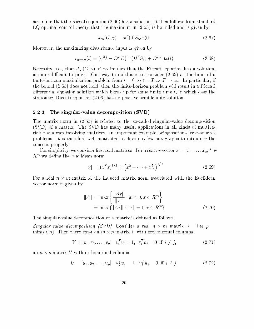
Singular-value decomposition (SVD). Consider a real n � m matrix A. Let p =min(m;n). Then there exist an m� p matrix V with orthonormal columns

V = [v1; v

2; : : : ; vp]; vTi vi = 1; vTi vj = 0 if i 6= j; (2.71)

an n� p matrix U with orthonormal columns,

U = [u1; u

2; : : : ; up]; uTi ui = 1; uTi uj = 0 if i 6= j; (2.72)

20

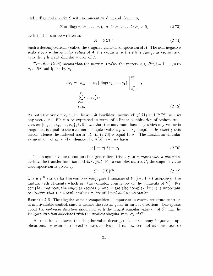
and a diagonal matrix � with non-negative diagonal elements,

� = diag(�1; �

2; : : : ; �p); �

1� �

2� : : : � �p � 0; (2.73)

such that A can be written asA = U�V T (2.74)

Such a decomposition is called the singular-value decomposition of A. The non-negativescalars �i are the singular values of A, the vector ui is the ith left singular vector, andvj is the jth right singular vector of A.

Equation (2.74) means that the matrix A takes the vectors vi 2 Rm; i = 1; : : : ; p toui 2 Rn multiplied by �i,

Avi = [ u1; : : : ; up ] diag(�1; : : : ; �p)

264vT1

...vTp

375 vi

=pX

k=1

�kukvTk vi

= �iui (2.75)

As both the vectors vi and ui have unit Euclidean norms, cf. (2.71) and (2.72), and asany vector x 2 Rm can be expressed in terms of a linear combination of orthonormalvectors fv

1; : : : ; vp; : : : ; vmg, it follows that the maximum factor by which any vector is

magni�ed is equal to the maximum singular value �1, with v

1magni�ed by exactly this

factor. Hence the induced norm kAk in (2.70) is equal to �1. The maximum singular

value of a matrix is often denoted by ��(A), i.e., we have

kAk = ��(A) = �1

(2.76)

The singular-value decomposition generalizes trivially to complex-valued matrices,such as the transfer function matrix G(j!). For a complex matrixG, the singular-valuedecomposition is given by

G = U�V H (2.77)

where V H stands for the complex conjugate transpose of V (i.e., the transpose of thematrix with elements which are the complex conjugates of the elements of V ). Forcomplex matrices, the singular vectors U and V are also complex, but it is importantto observe that the singular values �i are still real and non-negative.

Remark 2.5. The singular-value decomposition is important in control structure selection

in multivariable control, since it de�nes the system gains in various directions. One speaks

about the high-gain direction associated with the largest singular value �1of G, and the

low-gain direction associated with the smallest singular value �p of G.

As mentioned above, the singular-value decomposition has many important ap-plications, for example in least-squares analysis. It is, however, not our intention to

21

pursue these topics here. There are e�cient numerical algorithms for the singular-value

decomposition. An implementation is found in the program svd in MATLAB.The singular-value decomposition is not hard to prove, and due to its importance,

we give below an outline of how the result (2.74) can be shown.

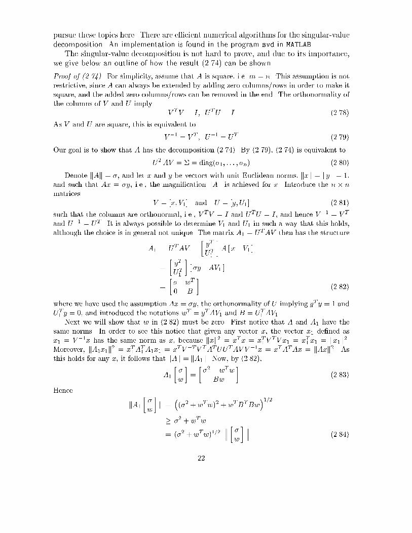
Proof of (2.74). For simplicity, assume that A is square, i.e. m = n. This assumption is not

restrictive, since A can always be extended by adding zero columns/rows in order to make it

square, and the added zero columns/rows can be removed in the end. The orthonormality of

the columns of V and U imply

V TV = I; UTU = I (2.78)

As V and U are square, this is equivalent to

V �1 = V T ; U�1 = UT (2.79)

Our goal is to show that A has the decomposition (2.74). By (2.79), (2.74) is equivalent to

UTAV = � = diag(�1; : : : ; �n) (2.80)

Denote kAk = �, and let x and y be vectors with unit Euclidean norms, kxk = kyk = 1,

and such that Ax = �y, i.e., the magni�cation kAk is achieved for x. Introduce the n � n

matrices

V = [x; V1] and U = [y; U

1] (2.81)

such that the columns are orthonormal, i.e., V TV = I and UTU = I, and hence V �1 = V T

and U�1 = UT . It is always possible to determine V1and U

1in such a way that this holds,

although the choice is in general not unique. The matrix A1= UTAV then has the structure

A1= UTAV =

�yT

UT1

�A [ x V

1]

=

�yT

UT1

�[ �y AV

1]

=

�� wT

0 B

�(2.82)

where we have used the assumption Ax = �y, the orthonormality of U implying yT y = 1 and

UT1y = 0, and introduced the notations wT = yTAV

1and B = UT

1AV

1.

Next we will show that w in (2.82) must be zero. First notice that A and A1have the

same norms. In order to see this notice that given any vector x, the vector x1de�ned as

x1= V �1x has the same norm as x, because kxk2 = xTx = xT

1V TV x

1= xT

1x1= kx

1k2.

Moreover, kA1x1k2 = xT

1AT1A1x1= xTV �TV TATUUTAV V �1x = xTATAx = kAxk2. As

this holds for any x, it follows that kAk = kA1k. Now, by (2.82),

A1

��

w

�=

��2 + wTw

Bw

�(2.83)

Hence

kA1

��

w

�k =

�(�2 + wTw)2 + wTBTBw

�1=2

� �2 + wTw

= (�2 + wTw)1=2 � �

w

� (2.84)

22

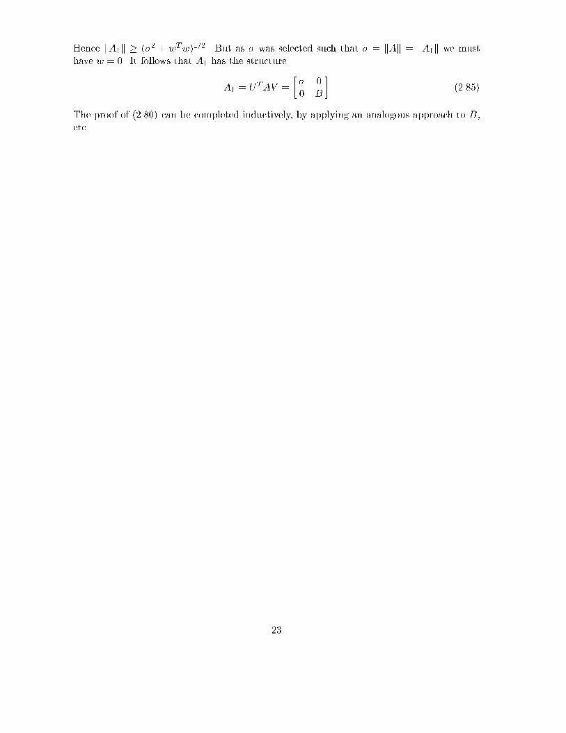
Hence kA1k � (�2 + wTw)1=2. But as � was selected such that � = kAk = kA

1k we must

have w = 0. It follows that A1has the structure

A1= UTAV =

�� 0

0 B

�(2.85)

The proof of (2.80) can be completed inductively, by applying an analogous approach to B,

etc.

23