Shrapnel motion

�

Christopher James Poole

University College

University of Oxford

A thesis submitted for the degree of

Master of Science

Trinity 2001

Acknowledgements

I would like to thank Dr John Ockendon for his patience and help through-

out the writing of this dissertation and to Dr Hilary Ockendon for her

suggestions on the development of the problem. I would also like to thank

Dr Chris Breward for kindly proof-reading some chapters. I am grateful

for Dr John Curtis in allowing me to study this problem and for QinetiQ’s

bursary, and the Engineering and Physical Sciences Research Council for

their pecuniary support. Finally, thanks to my family and friends for their

support and to the England cricket team in allowing me time to do my

work.

Abstract

When a bomb explodes, the bomb-casing breaks up causing shrapnel frag-

ments to scatter off with high velocity. Whilst study on penetration of

the designated target has been addressed, the mechanics involved in the

motion of the shrapnel have not been examined in great detail. This

dissertation will address shrapnel motion using ideas from gasdynamics.

The motivation for this problem comes from QinetiQ who, among other

things, play an active role in modelling violent mechanics.

Contents

1 Introduction 1

1.1 Motivation . . . . . . . . . . . . . . . . . . . . . . . . . . . . . . . . . 1

1.2 The shrapnel problem . . . . . . . . . . . . . . . . . . . . . . . . . . 2

1.3 Plan of dissertation . . . . . . . . . . . . . . . . . . . . . . . . . . . . 5

2 Background Fluid Mechanics 7

2.1 Basic ideas about incompressible flow . . . . . . . . . . . . . . . . . . 7

2.1.1 Boundary layers and turbulence . . . . . . . . . . . . . . . . . 9

2.1.2 Flow through a nozzle . . . . . . . . . . . . . . . . . . . . . . 11

2.1.3 Other pipe flows . . . . . . . . . . . . . . . . . . . . . . . . . 14

2.1.4 Inlet flow . . . . . . . . . . . . . . . . . . . . . . . . . . . . . 17

2.1.5 Orifices . . . . . . . . . . . . . . . . . . . . . . . . . . . . . . 19

2.1.6 Screens . . . . . . . . . . . . . . . . . . . . . . . . . . . . . . . 20

2.2 Compressible flow . . . . . . . . . . . . . . . . . . . . . . . . . . . . . 22

2.2.1 Shock waves . . . . . . . . . . . . . . . . . . . . . . . . . . . . 23

2.2.2 Rankine-Hugoniot jump conditions . . . . . . . . . . . . . . . 23

2.2.3 Conservation laws for compressible flow . . . . . . . . . . . . . 25

2.2.4 Thermodynamics background . . . . . . . . . . . . . . . . . . 26

2.2.5 Simple wave flow . . . . . . . . . . . . . . . . . . . . . . . . . 28

2.2.6 Shock tube . . . . . . . . . . . . . . . . . . . . . . . . . . . . 29

2.2.7 Basic control volume equations . . . . . . . . . . . . . . . . . 30

2.2.8 Pipe flows . . . . . . . . . . . . . . . . . . . . . . . . . . . . . 33

3 Models for shrapnel 44

3.1 Expanding gas causing piston motion into a vacuum . . . . . . . . . . 44

3.2 Porous Piston . . . . . . . . . . . . . . . . . . . . . . . . . . . . . . . 48

3.2.1 Incompressible flow and the porous piston . . . . . . . . . . . 48

3.2.2 Compressible flow and the porous piston . . . . . . . . . . . . 50

i

3.3 Rock blasting theory . . . . . . . . . . . . . . . . . . . . . . . . . . . 53

3.3.1 Cliff Blasting . . . . . . . . . . . . . . . . . . . . . . . . . . . 53

3.3.2 Existing model . . . . . . . . . . . . . . . . . . . . . . . . . . 55

3.3.3 Rock blasting theory applied to shrapnel . . . . . . . . . . . . 60

3.4 Comparison of the models . . . . . . . . . . . . . . . . . . . . . . . . 62

4 Conclusions 64

4.1 Summary of work . . . . . . . . . . . . . . . . . . . . . . . . . . . . . 64

4.2 Further work . . . . . . . . . . . . . . . . . . . . . . . . . . . . . . . 64

4.3 Final comments . . . . . . . . . . . . . . . . . . . . . . . . . . . . . . 65

Bibliography 66

ii

List of Figures

1.1 Bomb with preformed (man-made) fragments. . . . . . . . . . . . . . 2

1.2 The shrapnel problem. . . . . . . . . . . . . . . . . . . . . . . . . . . 2

1.3 Globe-shaped bomb casing from 1886. . . . . . . . . . . . . . . . . . 3

1.4 A sequence of photos showing bomb exploding, starting with the ‘det-

onator initiation’ and ending 20µs after detonation (from QinetiQ FP-

23 hi-speed photography). . . . . . . . . . . . . . . . . . . . . . . . . 4

1.5 A sequence leading to shrapnel motion. . . . . . . . . . . . . . . . . . 5

2.1 Streamlines. . . . . . . . . . . . . . . . . . . . . . . . . . . . . . . . . 8

2.2 Boundary layer separation - velocity profile. . . . . . . . . . . . . . . 10

2.3 Boundary layer separation. . . . . . . . . . . . . . . . . . . . . . . . . 11

2.4 Flow through a nozzle. . . . . . . . . . . . . . . . . . . . . . . . . . . 11

2.5 Flow through a nozzle (control volume). . . . . . . . . . . . . . . . . 12

2.6 Boundary layer separation and turbulence in a nozzle. . . . . . . . . . 14

2.7 A pipe with a gentle contraction. . . . . . . . . . . . . . . . . . . . . 14

2.8 A pipe with a gentle expansion. . . . . . . . . . . . . . . . . . . . . . 15

2.9 Flow through a pipe with a sudden contraction. . . . . . . . . . . . . 16

2.10 Flow through a pipe with a sudden expansion. . . . . . . . . . . . . . 17

2.11 Different inlet geometries. . . . . . . . . . . . . . . . . . . . . . . . . 18

2.12 Flow through an orifice. . . . . . . . . . . . . . . . . . . . . . . . . . 19

2.13 Flow past a screen. . . . . . . . . . . . . . . . . . . . . . . . . . . . . 20

2.14 Two screens with similar geometrical ratios leading to similar pressure

losses across the screen. . . . . . . . . . . . . . . . . . . . . . . . . . . 21

2.15 Loss factor K plotted against 1− S [16]. . . . . . . . . . . . . . . . . 22

2.16 A shock. . . . . . . . . . . . . . . . . . . . . . . . . . . . . . . . . . . 24

2.17 Shock tube before diaphragm bursts. . . . . . . . . . . . . . . . . . . 29

2.18 x− t diagram for a shock tube. . . . . . . . . . . . . . . . . . . . . . 29

2.19 A control volume in a pipe. . . . . . . . . . . . . . . . . . . . . . . . 31

2.20 Plot of A against M . . . . . . . . . . . . . . . . . . . . . . . . . . . . 34

iii

2.21 Laval Nozzle. . . . . . . . . . . . . . . . . . . . . . . . . . . . . . . . 34

2.22 A schematic showing velocity when At > Ac (so flow remains subsonic). 35

2.23 Area of throat At = Ac, hence sonic at the throat. . . . . . . . . . . . 36

2.24 Schematic of ∆p against M1, with choking limit shown. . . . . . . . . 36

2.25 A sequence of different outcomes, each diagram representing an in-

creasing value of ∆p. . . . . . . . . . . . . . . . . . . . . . . . . . . . 37

2.26 A diffuser. . . . . . . . . . . . . . . . . . . . . . . . . . . . . . . . . . 38

2.27 Sudden contraction with throat. . . . . . . . . . . . . . . . . . . . . . 38

2.28 Sudden expansion (no choking) [16]. . . . . . . . . . . . . . . . . . . . 39

2.29 Sudden expansion with a possible downstream shock structure. . . . . 40

2.30 Oblique shocks. . . . . . . . . . . . . . . . . . . . . . . . . . . . . . . 40

2.31 Sonic line (M = 1) shown for an orifice. . . . . . . . . . . . . . . . . . 41

2.32 Round-wire screen losses in high-velocity flow [8] (experimental). . . . 43

3.1 Piston pushed by expanding gas into a vacuum. . . . . . . . . . . . . 44

3.2 Characteristic Diagram. . . . . . . . . . . . . . . . . . . . . . . . . . 45

3.3 A plot showing (nondimensional) piston velocity as a function of (nondi-

mensional) time. . . . . . . . . . . . . . . . . . . . . . . . . . . . . . 47

3.4 A porous piston (screen). . . . . . . . . . . . . . . . . . . . . . . . . . 48

3.5 U(t) for incompressible flow. . . . . . . . . . . . . . . . . . . . . . . . 50

3.6 A porous piston (screen) with barrel shocks. . . . . . . . . . . . . . . 52

3.7 A porous piston (screen) with a shock to the right. . . . . . . . . . . 52

3.8 Elastic/plastic wave propagation leading to fracturing. . . . . . . . . 54

3.9 Rocks from the fully fractured cliff start to move, starting from the

right-hand face. . . . . . . . . . . . . . . . . . . . . . . . . . . . . . . 55

3.10 Cliff considered as a 2D model. . . . . . . . . . . . . . . . . . . . . . 57

3.11 Characteristic diagram for cliff fracturing. . . . . . . . . . . . . . . . 58

3.12 Graphs showing void fraction (scaled) and rock speed (scaled), as func-

tions of position for different values of time. The blue line indicates

the smallest time value, then working up to the olive line. γ is taken

to be 1.3. . . . . . . . . . . . . . . . . . . . . . . . . . . . . . . . . . 59

3.13 A snapshot of shrapnel velocity for a two-faced cliff with R = 1. . . . 61

iv

Chapter 1

Introduction

1.1 Motivation

When a bomb explodes, fragments of the metal casing which initially surrounded

the explosive mixture fly off with high velocity. The process of fragments forming is

known as fragmentation, the metal fragments being shrapnel. Fragmentation warhead

technology can be applied to many munition systems (e.g. detonation of bombs).

This provides the motivation for understanding the dynamics behind fragmentation.

If we can model how fragments form, fly off and penetrate their designated targets,

then more efficient warheads can be designed so as to optimise destruction of their

targets, whilst causing minimal unwanted damage. The study of fragmentation also

has high significance in safety studies of containers that could possibly explode (e.g.

pressurised containers containing explosive chemicals).

The problem of fragment penetration of a target has been studied in some detail,

whereas there has been relatively little study of fragment formation (which occurs

during the expansion of the casing) and subsequent motion of these fragments. Nu-

merical simulations on fragmentation, known as hydrocode models, exist [4], although

they cannot make accurate predictions of the fragmentation pattern owing to the

underlying material models lacking sophistication.

There are three main types of fragment warhead:

(i) Casings with fully preformed fragments on their outer surface (Fig. 1.1).

(ii) Casing with known pre-existing fracture lines.

(iii) So-called ‘naturally fragmenting’ warheads. These consist of a casing which

cracks naturally as a result of the explosion.

1

Figure 1.1: Bomb with preformed (man-made) fragments.

We are interested in modelling the flow of gas between the fragments in the early

stages following detonation (Fig. 1.2). The ideas from the solution to these models

can then hopefully be applied to all three types of casing. The mechanics of the break

up of the casing are being studied in an MSc dissertation [7], drawing analogies with

the notion of a shaped charge.

Figure 1.2: The shrapnel problem.

1.2 The shrapnel problem

A bomb basically consists of an explosive mixture surrounded by a metal casing. Two

main bomb geometries will be discussed in this dissertation; spherical and cylindrical.

Fig. 1.3 shows a spherical casing [1]. The holes in the bottom and top show where

the dynamite and fuse are inserted. Spherical bombs are usually detonated from the

2

centre. The casing in this example is made from lead although modern casings are

typically made from steel or sometimes aluminium.

Figure 1.3: Globe-shaped bomb casing from 1886.

The mechanism of the explosion is as follows. Initially, the explosive is detonated.

Combustion occurs (starting at the ignition point), turning the explosive into high

pressure gas. The gas pressure causes the casing to expand, at first elastically and

then plastically [23]. The expansion also causes fracturing to occur in the casing.

Cracks in the casing do not allow the gas to escape until the casing has expanded

to roughly twice its original diameter [3, 12, 22]. After the casing has fractured, the

high-velocity gas causes the casing to break up and form shrapnel. The gas then

accelerates the shrapnel, flowing in the gaps between the fragments (Fig. 1.2). Hence

the shrapnel flies off with high velocity. The gas flowing between the fragments and

the shrapnel motion will be referred to as the shrapnel problem. An example of this

process is shown in Fig. 1.4. The photographs show a cylindrical casing detonated

at one end. This explodes, with a detonation wave1 propagating down the cylinder.

G. I. Taylor’s paper of 1941 [23] takes a mathematical and experimental look

at one of the ideas mentioned above, namely a detonation starting at one end of a

cylindrical casing as in Fig. 1.4. The different stages of the detonation are discussed.

He then looks at the resultant flow and discusses fragment motion.

QinetiQ present further experimental evidence on a video which captures an ex-

plosion. As shown in Fig. 1.5, the motion occurs in four distinct phases. The first

1A detonation is a form of shock wave where a chemical reaction occurs locally near the shock.

3

Figure 1.4: A sequence of photos showing bomb exploding, starting with the ‘det-onator initiation’ and ending 20µs after detonation (from QinetiQ FP-23 hi-speedphotography).

picture, (a), represents a small section of the casing before the combustion of the

explosive has occurred.

At the next time step, (b), we can see a jet starting to form from between the pre-

formed fragments. This is a consequence of the detonation wave having propagated

from the explosive mixture.

These jets grow to roughly three times their previous length in stage (c). In this

stage, the jets merge. Particle motion is then observed in (d). After this stage, we can

see a jagged leading-edge on the outside of the casing, although the gases obscure the

bulk of the particle motion. This indicates that the gas has rushed through the gaps

between the fragments and is now moving ahead of the fragments with high velocity.

Finally, everything on the video becomes unclear as a result of the gas obscuring the

motion.

We can compare the video evidence to the photography in Fig. 1.4, although the

latter is for a cylindrical casing. The same principles of shrapnel motion will apply for

4

Figure 1.5: A sequence leading to shrapnel motion.

each type of casing, whether it is cylindrical or spherical with pre-formed or natural

fragmentation.

1.3 Plan of dissertation

The background material on the subject is so sparse that the literature review will

be integrated into the following chapters.

In chapter 2, where we discuss fluid flow, we will open with a brief background

to incompressible flows. This will include a basic look at the equations and ideas

governing such flows, including Navier-Stokes equations, Bernoulli’s theorem, irrota-

tional flow and vorticity. We will then move on to boundary layers, boundary layer

separation and turbulence. These ideas will be applied to a nozzle with slowly-varying

cross-sectional area, introducing the concept of a head loss. Pipe flows, inlets, orifices

and screens will be reviewed, discussing head losses in each case. The second half of

this chapter will be devoted to compressible flows. We will take a look at conserva-

tion laws, Rankine-Hugoniot conditions and some thermodynamics. We will complete

the section on compressible flow background by looking at simple wave flow. These

ideas will be used in a discussion of the shock tube and possible ‘jump’ conditions.

We will then consider choked flow, before trying to generalise the specific situations

considered for incompressible flow to end the chapter.

5

In chapter 3, we will attempt to bring these ideas together and set up some models

of shrapnel motion. The first approach will model shrapnel as a piston expanding

into a vacuum. This idea will be made more sophisticated in the second approach

where we allow the piston to be porous. We will attempt to develop models for the

incompressible case first, in order to gain intuition, and then go on to the compressible

cases. The final model will use ideas from the theory of rock-blasting and consider

how they might be applied to the shrapnel problem. We will complete this chapter

by comparing the various models.

In chapter 4, we will give an overview of the dissertation and discuss possible

modifications and future work to be carried out on the subject.

6

Chapter 2

Background Fluid Mechanics

We need to establish a detailed background on fluid mechanics to give us the in-

frastructure to develop a model on shrapnel motion. We aim to model the shrapnel

problem for compressible gases. To gain intuition, we will firstly look at incompress-

ible flow and then transfer ideas across to compressible flow. The simplest idea would

be to consider these flows for 1-dimensional problems. This motivates the following

sections.

2.1 Basic ideas about incompressible flow

A flow is incompressible if the density ρ of the fluid is constant everywhere. This

section is devoted to a study of such flows, starting with a few preliminaries.

A good starting place for discussing incompressible flows is with the Navier-Stokes

equations, which are well documented in any good fluid mechanics textbook [2]:

ρ( ∂

∂t+ (u.∇)

)u = −∇p + µ∇2u (2.1)

∇.u = 0 (2.2)

where ρ is the fluid density, u the fluid velocity, p the pressure and µ is the viscosity,

which is assumed constant. We have neglected gravity in (2.1). These equations will

hold throughout the fluid. The first of the equations (2.1), which is clearly nonlinear,

can be derived by looking at conservation of momentum for a material volume of the

fluid. The second of the two equations (2.2) is conservation of mass. This is easily

derived by considering fluid flux across a volume V .

An inviscid fluid flow is one where viscous effects of the fluid are neglected. Hence

(2.1) reduces to ( ∂

∂t+ u.∇

)u = −1

ρ∇p. (2.3)

7

This is known as Euler’s equation. Assuming steady flow ( ∂∂t

= 0) and using vector

identities, this can be written as

(∇ ∧ u) ∧ u = −∇(p

ρ+

1

2u2). (2.4)

A streamline is a curve which has the same direction as u at any time (Fig. 2.1).

Taking the dot product of (2.4) with u we obtain

Figure 2.1: Streamlines.

(u.∇)(p

ρ+

1

2u2) = 0. (2.5)

Hence for steady flow,

(p

ρ+

1

2u2) = constant on a streamline. (2.6)

This is Bernoulli’s equation.

We now introduce the vorticity of the fluid, defined by

ω = ∇ ∧ u. (2.7)

It can be shown [2] by considering the circulation Γ =∫

Cu.dx around a closed curve

C that if ω = 0 at t = 0, then ω = 0 for all time. This is the Cauchy-Lagrange

theorem.

A flow with ω = 0 is defined as irrotational flow. A special case of Bernoulli’s

equation arises in irrotational flow. Clearly, (2.4) reduces to

∇(p

ρ+

1

2u2) = 0, (2.8)

which means that the quantity (pρ

+ 12u2) is constant throughout the fluid.

8

2.1.1 Boundary layers and turbulence

If we used the inviscid theory outlined above for flow past a rigid body, the fluid

which comes in contact with the object would just slip past the object. This may

give a good idea of the flow in general, but is in fact incorrect if we look more closely.

We can nondimensionalise (2.1) in the form [18]( ∂

∂t+ (u.∇)

)u = −∇p +

1

Re∇2u (2.9)

where

Re =UL

ν(2.10)

is the Reynolds number (nondimensional), U , L typical velocity and length scales

and ν = µρ

the kinematic viscosity. u, ∇ , p and t in (2.9) are now nondimensional.

For 1Re� 1, we have a boundary layer. This is a thin layer of the fluid in which the

fluid velocity changes rapidly from zero on the object to match in with the main fluid

flow outside this layer. The mathematics can be demonstrated by using an ordinary

differential equation1:

εdu

dt− u = −1, (2.11)

with boundary condition

u(0) = 0, (2.12)

ε � 1. Here, the parameter ε is like 1Re

(very small). Naively neglecting the ε term

leads to the solution u = 1. This does not satisfy the boundary condition imposed.

The remedy is to rescale x so that the ε term was of importance (e.g. x = εX,

u(x) = U(X), then solve for U(X)). Our boundary layer, where rapid changes occur,

is near x = 0, of thickness ε. The same idea holds for the fluid - if we get sufficiently

close to the boundary of the body, we have a boundary layer where the viscous effects

will become important. An analysis of the boundary layer is possible by rescaling u

and p. Suitable scalings involving Re for different flow regimes allow us to get good

approximations in the boundary layers and in the main flow.

Clearly, the introduction of viscosity would not affect the incompressibility equa-

tion (2.2). It does mean, however, that we cannot use Euler’s equation and must

use the full Navier-Stokes equation (2.1). We use the nondimensional version (2.9),

assuming steady flow ( ∂∂t

= 0). One component of our equation is

u∂u

∂x+ v

∂u

∂y= −∂p

∂x+

1

Re

(∂2u

∂x2+

∂2u

∂y2

). (2.13)

1A singular perturbation problem.

9

In the boundary layer, the viscous forces become more important, hence we wish to

balance them with the pressure gradient (as we are looking at the shear in the x

direction). We rescale [18]

y =Y√Re

(2.14)

and hence, by incompressibility (2.2),

v =V√Re

(2.15)

to obtain the boundary layer equation(u

∂

∂x+ V

∂

∂Y

)u = −∂p

∂x+

∂2u

∂Y 2. (2.16)

Note that we almost have Euler’s equation, apart from now we have a ∂2u∂Y 2 term

which is of the same order as the other terms in the boundary layer. This viscous

term means that we get different solutions in the boundary layer than in the main

flow.

Boundary layers can be laminar or turbulent, but either can separate from the

boundary under certain circumstances. Boundary layer separation can cause the

whole flow of a low-viscosity fluid to change completely. Adverse pressure gradients

Figure 2.2: Boundary layer separation - velocity profile.

in the outer flow cause the flow to reverse near the boundary (Fig. 2.2) and this is

observed to always lead to separation. The separation can lead to the formation of

wakes behind the body (Fig. 2.3). The flow profile of Fig. 2.2 is slightly unrealistic

in practice and we are more likely to get triple deck flow near the separation point.

10

Figure 2.3: Boundary layer separation.

Details are beyond the scope of this dissertation, though can be found in Ockendon

& Ockendon [18].

Separation can lead to turbulence in the main body of the flow. Turbulence is

difficult to define. An area of turbulent flow will consist of vortices and eddies of

many shapes and sizes, with the fluid particles following irregular paths. Turbulent

flow is the opposite of laminar flow and is most easily generated from a strong shear.

Two well-known examples of turbulence occurring owing to instabilities are Rayleigh-

Taylor instability (denser fluid on top of a less dense one) and Kelvin-Helmholtz

instability (layered fluids, with the upper layer of lower density flowing over the lower

layer) [2].

2.1.2 Flow through a nozzle

(i) Inviscid theory

The first flow we shall consider is flow through a nozzle, shown in Fig. 2.4

Figure 2.4: Flow through a nozzle.

11

As shown, neglecting viscosity, the flow will accelerate through the contracting

part of the nozzle and decelerate as the nozzle expands. Considering the nozzle

as a 2-dimensional model, we wish to obtain a slowly-varying solution of Euler’s

equation (2.3) with (inviscid) boundary conditions u.n = 0 holding on the

nozzle boundary, n being the normal to the nozzle. Denote upper and lower

edges of the nozzle by y = h+(x) and y = h−(x) respectively. Writing the fluid

velocity u = (u, v) in the usual manner, the boundary condition is

v = uh′± on y = h±. (2.17)

We wish to solve∂u

∂x+

∂v

∂y= 0 (2.18)

with boundary conditions, so integrating between h− and h+ with respect to y

and using the boundary conditions we obtain

∂

∂x(u(h+ − h−)) = 0. (2.19)

Rewriting the difference in heights (h+ − h−) as Aα for α = 1, 2, and taking a

control volume of fluid (Fig. 2.5) we obtain conservation of mass in the form

A1u1 = A2u2 = Q, (2.20)

where Q is constant. Note that we can also apply the same idea to a 3-

dimensional problem.

Figure 2.5: Flow through a nozzle (control volume).

We can obtain another control volume equation by observing that Bernoulli’s

equation (2.6) will hold on the centre streamline (laminar flow). In terms of our

control volume subscripts, this says

p1 +1

2ρu2

1 = p2 +1

2ρu2

2. (2.21)

12

A final balance is obtained by integrating

∇p + ρ(u.∇)u = 0 (2.22)

over the control volume region, V , with boundary S. This gives∫S

(pn + ρu(u.n))dS = 0. (2.23)

Hence the total force on the control volume is equal to the momentum flux from

S. As the nozzle is assumed to be slowly varying, however, we know u.n = 0

on y = h±. Including the drag of the nozzle, this becomes

(p1 + ρu21)− (p2 + ρu2

2) = Drag on nozzle. (2.24)

(ii) Viscous effects, Re� 1

Experimentally, however, we sometimes obtain different results than the above.

In particular, we note that Bernoulli is violated and

p1

ρg+

u21

2g=

p2

ρg+

u22

2g+ hs, (2.25)

where hs is the head loss. The size and importance of this term depends very

much on the geometry of the model. This can be rewritten as

hs =p1 − p2

ρg+

u21 − u2

2

2g. (2.26)

We need to reconcile this equation with the nozzle flow. Hence we introduce a

viscosity term, though still remembering that our flow is not very viscous (so

Re� 1).

In the case of the nozzle, boundary layers form on the edge surface in the section

of decelerating flow as shown in Fig. 2.6. These layers can separate as a result

of the adverse pressure gradient on the edge of the expanding part, leading to

turbulence in the bulk flow and hence causing the head loss term hs in (2.25).

In general, the loss coefficient (or loss factor) is defined in terms of hs as [5]

hs = Ku2

2

2g(2.27)

for some constant K, hence

(p1

ρ+

1

2u2

1)− (p2

ρ+

1

2u2

2) =1

2Ku2

2. (2.28)

Although we can write the loss in terms of the upstream velocity by (2.20), we

choose to use the downstream velocity as the turbulent flow leading to the loss

is downstream.

13

Figure 2.6: Boundary layer separation and turbulence in a nozzle.

2.1.3 Other pipe flows

(i) Gentle Contraction

A gentle contraction as shown in Fig. 2.7 is perhaps one of the easiest cases

to look at. Mass conservation in the form (2.20) will obviously hold for

the contracting pipe, with control volume boundaries denoted by 1 and 2.

Also, as the pipe is contracting gently, there will not be any significant flow

separation at the walls of the pipe. Hence we will not get any significant

departure from inviscid flow and so we expect (2.21) to remain true. This

is experimentally confirmed to be the case in engineering literature [5].

The only error we might get would arise from friction in (2.23).

Figure 2.7: A pipe with a gentle contraction.

14

(ii) Gentle Expansion

Figure 2.8: A pipe with a gentle expansion.

Fig. 2.8 shows a gentle pipe expansion. Mass conservation will hold in

the form (2.20). The separation of the boundary layers leads to some

turbulence in the middle of the pipe, disrupting the laminar flow. This

will lead to a head loss. Thus (2.28) will hold for some K. The size of

K will not be very large in this case, as the pipe cross-sectional area is

only slowly varying. This implies that the size of hs will not be very large

compared to the other terms in (2.25). Analysis on curvature in pipes [21]

suggests that this value will be negligible (K ∼ 0.04 for a smooth bend),

and hence we can realistically apply (2.21).

(iii) Sudden contraction

Fig. 2.9 shows a typical pipe contraction. 1, c and 2 refer to control

volume subscripts which we shall refer to in the following text. The flow is

divided into two regions [17], one of laminar flow and one where turbulence

occurs. Firstly, the fluid accelerates through the contraction. The laminar

structure of the flow is maintained (no turbulence) in this part of the flow.

Separation of shear layers then starts to occur. A vena contracta, with

cross-sectional area Ac, forms as shown. This is the minimum area through

which the fluid flows (like a neck). After this area, we effectively have an

expansion. Shear layers separate, leading to turbulence and hence a head

loss hs and a loss factor K. Define the contraction coefficient by

Cc =Ac

A2

. (2.29)

15

Figure 2.9: Flow through a pipe with a sudden contraction.

For a ratio of A2

A1= 0.1, then it is found experimentally that [17] Cc ∼ 0.62.

This leads to K ≈ 0.37. A range of values are published in [24], shown in

the following table. Note the low value of K for a high ratio of A2

A1. This

reinforces the argument for a pipe with a gentle contraction that K can

almost be neglected.

A2/A1 K0.1 0.370.2 0.350.3 0.320.4 0.270.5 0.220.6 0.170.7 0.100.8 0.060.9 0.021.0 0

For a pipe with no drag, it is experimentally confirmed [5, 13, 17] that

K =(A2

Ac

− 1)2

=( 1

Cc

− 1)2

(2.30)

is a good approximation for K.

(iv) Sudden expansion

We expect a sudden expansion (Fig. 2.10) to be more dramatic than

the gentle expansion. Once again, we use our general principles and see

16

at once that conservation of mass (2.20) must hold. We also have shear

layers separating, causing turbulence which will stop the incoming flow

from remaining laminar. Thus we expect there to be a significant head

loss hs and (2.28) will hold.

An experimental form for K is given by [5, 13, 17] as

K =(A2

A1

− 1)2

. (2.31)

Figure 2.10: Flow through a pipe with a sudden expansion.

2.1.4 Inlet flow

Consider flow from a (relatively) large vessel into a small opening in the wall of

the vessel. This opening is an inlet (Fig. 2.11). We are interested in finding loss

coefficients for inlets as we can think of the gas flowing into the inlet as gas flowing

between shrapnel fragments. The following arguments apply to stationary inlets. The

ideas, however, will still follow for shrapnel (which moves) as the shrapnel will not be

moving as fast as the high-speed gas.

We obtain values of the loss coefficient K experimentally [17]. It is found that

they are strongly dependent on the geometry of the inlet. For the purpose of clarity of

the Fig. 2.11, turbulent motion resultant from shear layer separation is not drawn on

the diagrams, though it should be stressed again that this is the reason for Bernoulli’s

equation not holding, hence the loss factor K. Note that the strength of the separation

force on shear layers will correlate with the effect (and amount) of head loss.

17

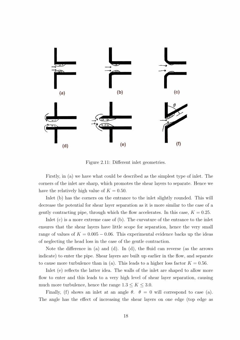
Figure 2.11: Different inlet geometries.

Firstly, in (a) we have what could be described as the simplest type of inlet. The

corners of the inlet are sharp, which promotes the shear layers to separate. Hence we

have the relatively high value of K = 0.50.

Inlet (b) has the corners on the entrance to the inlet slightly rounded. This will

decrease the potential for shear layer separation as it is more similar to the case of a

gently contracting pipe, through which the flow accelerates. In this case, K = 0.25.

Inlet (c) is a more extreme case of (b). The curvature of the entrance to the inlet

ensures that the shear layers have little scope for separation, hence the very small

range of values of K = 0.005− 0.06. This experimental evidence backs up the ideas

of neglecting the head loss in the case of the gentle contraction.

Note the difference in (a) and (d). In (d), the fluid can reverse (as the arrows

indicate) to enter the pipe. Shear layers are built up earlier in the flow, and separate

to cause more turbulence than in (a). This leads to a higher loss factor K = 0.56.

Inlet (e) reflects the latter idea. The walls of the inlet are shaped to allow more

flow to enter and this leads to a very high level of shear layer separation, causing

much more turbulence, hence the range 1.3 ≤ K ≤ 3.0.

Finally, (f) shows an inlet at an angle θ. θ = 0 will correspond to case (a).

The angle has the effect of increasing the shear layers on one edge (top edge as

18

shown in the diagram) and decreasing it on the other. K is given empirically by

K = (0.5 + 0.3 cos θ + 0.2 cos2 θ).

Depending on the Reynolds number, the flow may or may nor become approxi-

mately laminar sufficiently far downstream. Hence, in addition to the experimental

values given above, additional losses in the pipe will occur downstream before we get

laminar flow (if it does occur), which is usually in about the first 30 pipe diameters.

These losses often add about 0.1 to the loss coefficient K.

2.1.5 Orifices

Figure 2.12: Flow through an orifice.

An orifice (Fig. 2.12) is a plate with a small, sharp-edged hole, placed in a flowing

stream [10]. The motivation for considering an orifice is similar to the motivation for

inlets. Gas flow past fragments in a casing will pass through small gaps, which we

model here as a fixed orifice. Once again, even though the shrapnel will be moving,

it will not have a velocity as high as the high-speed gas, hence we can gain insight by

looking at the fixed orifice.

As the flow passes through the orifice, we will very quickly switch from a contrac-

tion to a very large expansion. Shear layers separate, leading to turbulence and a

head loss.

Sharp-edged orifices with area ratios A2

A1from 0.05 to 0.70 fit in well at high orifice

Reynolds numbers with the relation [10]

K = 1.6(1−

(A2

A1

)2). (2.32)

In this case, we can (if we wish) substitute K back into (2.28), rearrange and get

p1 + 1.3ρu21 = p2 + 1.3ρu2

2. (2.33)

19

i.e.

[p + 1.3ρu2]21 = 0. (2.34)

2.1.6 Screens

In the shrapnel problem, we will need to consider gas flow around many small frag-

ments. This motivates looking at a screen.

A screen (Fig. 2.13) can be defined [8] as a collection of elements which forms a

permeable sheet. This sheet is relatively thin in the direction of the flow through it.

The gas flow accelerates through the gaps in the screen, forming jets of high velocity

behind the holes. “Wakes” will form between the holes on the downstream side of

the screen. These are areas of the fluid where the velocity is lower than in the jets.

We will have eddies and turbulence in the wakes. Once again, further downstream,

depending on the Reynolds number, the jets will mix with the wakes, eventually

leading to uniform flow. It is found experimentally that this mixing process provides

the main contribution to the pressure losses across the screen.

Figure 2.13: Flow past a screen.

It is found by Miller [16] that a number of geometrical parameters of the screen

are not important, given that the separation and reattachment (where the jets and

wakes come back together) of the flow are the same for each element of the screen.

This means that we may effectively treat the screen as an array of pipes. For example,

loss coefficients for orifice plates and perforated plates are similar if ratios of total

orifice area to pipe area are the same (Fig. 2.14).

Also, for the same ratio of orifice to pipe area, the total vena contracta area is

similar irrespective of whether there are single or multiple orifices. However, for a

single orifice, the length of the outlet pipe required for full static pressure recovery

greatly exceeds the length required for multiple orifices.

20

Figure 2.14: Two screens with similar geometrical ratios leading to similar pressurelosses across the screen.

An important parameter when discussing screens is the solidity of the screen,

defined as the ratio

S =Blockage area of screen

Area of pipe or passage. (2.35)

If we can obtain an expression for the loss K in terms of S, then we should have be

able to get good estimates for K for different screens. Experimentally [16], values for

round wire screens with the Reynolds number Re > 500 have been obtained, and are

shown in Fig. 2.15.

Much investigation has been done on drag forces on screens owing to uses they

have in the aerodynamics industry (e.g. in engines). One hypothesis [5] for the drag

force D across the screen is

D = CdAblocked

(ρu2

2g

)(2.36)

where Cd is the drag coefficient of the screen and Ablocked the total blockage area of

the screen. This relationship is generally found to be true (and the notion of a drag

coefficient is not specific to screens.) The drag coefficient will be dependent on the

geometry of the screen. It will also depend on the nature of the wakes which form

downstream of the screen elements. Consider if the wakes are ‘closed’ (that is, they

terminate and the flow becomes approximately laminar further downstream). The

drag will depend on whether the wakes are stagnant (hence at stagnation pressure) or

whether there are eddies in the wakes. If the latter holds, we can find (experimentally)

a value for Cd which will depend on the screen element size and geometry. If the flow

in the wakes is stagnant, the drag force will be as if the screen element and wake are

one fixed body, and the drag will act around the boundary of the combined screen

element and closed wake (as the pressure acting on the screen element from behind

is negligible to that acting on the front).

21

Figure 2.15: Loss factor K plotted against 1− S [16].

Relationships between Cd and Re are known for low Reynolds number situations

(Re < 5) [6]. This does not interest us much as we will be considering high Reynolds

number flow.

2.2 Compressible flow

Up until now, we have only considered the fluid as being incompressible. This was

done for simplicity. The shrapnel problem, however, will involve compressible flow.

Hence, it will be more realistic to consider compressible flows in different geometries.

A marked contrast between incompressible and compressible flows is that we can have

shock waves forming in compressible flow, with Rankine-Hugoniot conditions holding

across the shocks.

22

2.2.1 Shock waves

Consider a curve C across which some gasdynamic quantity (such as density) has dis-

continuities. The usual system of first order conservation laws cannot be interpreted

over this curve as the first derivatives are not well-defined here. However, by stitching

together classical solutions2 across this curve, we can describe finite discontinuities

(jumps) in the solution. These finite discontinuities in the solution are known as

shocks. From a mathematical viewpoint, we note that by introducing shocks, we can

avoid the solution from being multi-valued.

2.2.2 Rankine-Hugoniot jump conditions

There can be different values of gasdynamic quantities either side of a shock wave.

We wish to derive a relationship between these different values. To do this, we derive

Rankine-Hugoniot jump conditions across a shock by looking at conservation laws.

Let P be some conserved quantity (such as mass or momentum) with flux Q, both

functions of x and t. We can derive a conservation law by looking at balances in a

region D in the (x, t) plane, whose boundary is C. This is done in [19], with the

result ∫C

Pdx−Qdt = 0 (2.37)

and the corresponding partial differential equation

∂P

∂t+

∂Q

∂x= 0. (2.38)

The latter is a conservation law.

Now rewrite (2.37) asd

dt

∫ B

A

Pdx = −[Q]BA (2.39)

for points A and B being points representing the boundary of some fixed region V .

Consider a shock, S, in the (x, t) plane. If we take A = S and B = S + δS as in

Fig. 2.16, we obtain

[P− − P+]δS ≈ −[Q]+−δt. (2.40)

Hence the shock speed will be given by

dS

dt=

[Q]+−[P ]+−

. (2.41)

2A classical solution of an nth order partial differential equation has to satisfy the partial differ-ential equation and be n times continuously differentiable.

23

Figure 2.16: A shock.

Unfortunately, this approach does have its limitations. Suppose it was applied to

the equation∂u

∂t+

∂

∂x(1

2u2) = 0. (2.42)

We would then get an expression for the shock speed as

U =[12u2]+−

[u]+−. (2.43)

We can also rewrite (2.42) as

∂

∂t(1

2u2) +

∂

∂x(1

3u3) = 0, (2.44)

which would clearly lead to the shock speed being given by

U =[13u3]+−

[12u2]+−

6=[12u2]+−

[u]+−. (2.45)

This shows that two conservation equations can be identical for smooth solutions

though can have different solutions if we allow shocks!

A further property of these jump conditions is that we can have nonuniqueness of

solutions for initial value problems. This can occur easily even for (2.42). Consider

(2.42) with initial conditions

u(x, 0) =

{1 x > 00 x < 0

. (2.46)

24

One possible solution is

u(x, t) =

1 x > txt

t > x > 0.0 0 > x

(2.47)

However, another solution is

u(x, t) =

{1 x > t

2

0 x < t2

, (2.48)

with the Rankine-Hugoniot condition

dx

dt=

[12u2]+−

[u]+−=

1

2, (2.49)

hence we have nonuniqueness of the solution of the initial value problem.

2.2.3 Conservation laws for compressible flow

As was the case in the incompressible flow regime, we need to start with the con-

servation laws for compressible flow. We assume 1-dimensional flow, and obtain the

conservation laws for mass, momentum and energy can be written as follows in con-

servation form (respectively) [19]:

∂ρ

∂t+

∂(ρu)

∂x= 0 (2.50)

∂(ρu)

∂t+

∂(p + ρu2)

∂x= 0 (2.51)

∂(ρe + 12ρu2)

∂t+

∂(ρue + 12ρu3 + pu)

∂x= 0, (2.52)

where e is the internal energy per unit mass of the gas.

Hence from (2.41) we can write the shock speed U as

U =[ρu]+−[ρ]+−

(2.53)

U =[p + ρu2]+−

[ρu]+−(2.54)

U =[ρue + 1

2ρu3 + pu]+−

[ρe + 12ρu2]+−

. (2.55)

25

Rearranging, and assuming [u]+− 6= 0 3, we arrive at the following Rankine-Hugoniot

shock relations:

[ρ(U − u)]+− = 0 (2.56)

[p + ρ(U − u)2]+− = 0 (2.57)

[h +1

2(U − u)2]+− = 0 (2.58)

where h = e + pρ

is the enthalpy. Note that we don’t need any area considerations

as we had in (2.20) because shocks are so thin. Furthermore, these equations just

express conservation of mass, momentum and energy across the shock (as the velocity

term u− U is relative to the shock).

2.2.4 Thermodynamics background

Suppose we heat a gas. Denote the heat addition per unit mass by Q. The equation

of conservation of energy (2.52), neglecting any conduction in the gas, generalises to

[19]

ρde

dt=

p

ρ

dρ

dt+ ρ

dQ

dt(2.59)

orde

dt+ p

d

dt

(1

ρ

)=

dQ

dt(2.60)

where ρ is gas density, p pressure and u the velocity. For most perfect gases, it is

experimentally confirmed that e = cvT , where T is the temperature and cv specific

heat at constant volume, assumed constant.

For a perfect gas, we have the relationship

p = ρRT (2.61)

which is confirmed experimentally for a gas at rest. Here, R is the gas constant, equal

to cp− cv where cp is the specific heat of constant pressure, assumed constant. Define

γ = cp

cv> 1 (γ = 5

3for a monatomic gas). We will use this notation frequently later.

Using these relations, we can rewrite (2.60) in the more useful form

d

dtlog

( p

ργ

)=

(γ − 1)

pρdQ

dt=

(γ − 1)

R

1

T

dQ

dt. (2.62)

We now define the entropy by

TdS

dt=

dQ

dt(2.63)

3[u]+− = 0 occurs in the case of a contact discontinuity, to be discussed later.

26

As we are working on an absolute temperature scale, T > 0. Also, as Q is the heat

supplied volumetrically, we must have dQdt

> 0. Hence dSdt

> 0, so entropy increases.

Combining (2.62) with this result and integrating, we obtain

p

ργ= exp

(S − S0

cv

)(2.64)

where S0 is a constant of integration.

Note that if there is no internal source term (Q = 0), then we have dSdt

= 0. This

gives us the result that the entropy of a fluid particle is constant (isentropic flow).

We have discussed various conservation laws and their effect on jump conditions.

We have not, however, considered what happens to the entropy across a shock. Using

subscripts 1 for upstream, 2 for downstream, assuming the shock travels from region

2 to region 1, we can rearrange (2.56), (2.57) and (2.58) to get

ρ2

ρ1

=(γ + 1)M2

1

2 + (γ − 1)M21

(2.65)

where M1 = U−u1

a1is the upstream Mach number and a2 = γp

ρ. Further, (2.57) and

(2.58) together lead to

p2

p1

=2γM2

1 − (γ − 1)

γ + 1. (2.66)

Hence the entropy jump across a shock is obtained by considering(p2

ργ2

)(ργ1

p1

)=

(p2

p1

)(ρ1

ρ2

)γ

=(1 +

2γ

γ + 1(M2

1 − 1))(1 + (γ−1

γ+1)(M2

1 − 1)

1 + (M21 − 1)

)γ

. (2.67)

For values of the upstream Mach number M1 near to 1, we may set M21 − 1 = ε

and expand the above expression asymptotically to get(p2

p1

)(ρ1

ρ2

)γ

= 1 +2γ(γ − 1)

3(γ + 1)2ε3 + O(ε4) (2.68)

and hence the entropy jump is given as

S2 − S1

cv

= log(p2

ργ2

)− log

(p1

ργ1

)= O(ε3)

= O((p2 − p1

p1

)3)

(2.69)

by (2.66).

Interestingly, the result above gives us that we must have M1 > 1 as the entropy

must increase.

27

2.2.5 Simple wave flow

The final idea we will need is the concept of simple wave flow, which will be defined

later in this section. The 1-dimensional conservation laws (2.50), (2.51) and (2.52)

for homentropic4 flow can be written as

∂ρ

∂t+

∂

∂x(ρu) = 0 (2.70)

ρ(∂u

∂t+ u

∂u

∂x) = −∂p

∂x(2.71)

p

ργ=

p0

ργ0

= constant, (2.72)

where p0 and ρ0 (assumed constant) are stagnation values of p and ρ.

Defining the speed of sound a for an isotropic flow by

a2 =γp

ρ, (2.73)

the conservation laws reduce to

∂a

∂t+ u

∂a

∂x+

γ − 1

2a∂u

∂x= 0 (2.74)

∂u

∂t+ u

∂u

∂x+

2a

γ − 1

∂a

∂x= 0. (2.75)

We now have a system of partial differential equations in a and u. We can diago-

nalise the system using matrix algebra in the form

( ∂

∂t+ (u± a)

∂

∂x

)(u± 2a

γ − 1) = 0. (2.76)

This shows that

u± 2a

γ − 1= constant on

dx

dt= u± a. (2.77)

u± 2aγ−1

are the Riemann invariants of the system, with characteristics dxdt

= u±a. We

will refer to these characteristics as C±. Depending on the boundary conditions and

geometry, one family of characteristics can reduce to straight lines. This is simple

wave flow.

When modelling shrapnel motion, we can consider the shrapnel as having no mass,

but as a discontinuity between two regions. This motivates the next section on a shock

tube, which will use ideas from simple wave flow and from section 2.2.2.

4A homentropic flow is one where the entropy S of all the fluid particles is constant for all time(cf. homo+entropy, Greek)

28

2.2.6 Shock tube

A shock tube is a tube consisting of, initially, two different regions, one of high pressure

(compression chamber) and one of low pressure (expansion chamber). The regions

are initially segregated by a diaphragm at x = 0, say (Fig. 2.17).

Figure 2.17: Shock tube before diaphragm bursts.

At time t = 0, the diaphragm is burst. The subsequent flow is divided into 4

different regions, labelled 1-4 as in Fig. 2.18. The interface between regions 2 and 3

is known as a contact discontinuity (or contact surface). It is the boundary between

the fluids which were initially on opposite sides of the diaphragm. These fluids,

neglecting any diffusion, will remain separated throughout the motion.

Figure 2.18: x− t diagram for a shock tube.

29

We have jump conditions across the discontinuity:

[p]32 = [u]32 = 0

[T ]32 6= 0 6= [ρ]32. (2.78)

The boundary between regions 3 and 4 is a shock wave. We use Rankine-Hugoniot

conditions (2.56), (2.57) and (2.58) across the shock (with U = 0) to give the following

well-documented relations [14]

ρ3

ρ4

=u4

u3

=1 + γ4+1

γ4−1p3

p4

γ4+1γ4−1

+ p3

p4

(2.79)

where subscripts denote the quantities in the different regions.

Further analysis which we omit here (though can be found in [14]) leads to the

relationship

u3 = a4

(1− p3

p4

)√√√√ 2γ4

(γ4 + 1)p3

p4+ γ4 − 1

. (2.80)

We now consider the boundary between regions (1) and (2), using our arguments

on simple wave flow. By homentropy,

ρ = ρ1

( a

a1

) 2γ−1

. (2.81)

The C+ characteristics leave (1) and enter (2), so using (2.81), we arrive at

u2 =2a1

γ1 − 1

((p2

p1

) γ1−12γ1 − 1

). (2.82)

Finally, imposing the conditions (2.78), we find a value for the velocity of the contact

discontinuity.

2.2.7 Basic control volume equations

Ideally, this section would mirror the incompressible analysis and look at the cases

of sudden expansions, contractions, inlets, orifices and screens as in sections 2.1.3,

2.1.4, 2.1.5 and 2.1.6. Literature does exist on pressure losses in screens and we will

consider this in due course. Firstly, we need to consider what our jump conditions

will be across a control volume.

30

For steady compressible flow, conservation of mass and momentum can be written

∇.(ρu) = 0 (2.83)

ρ(u.∇)u = −∇p. (2.84)

We consider a 2-dimensional control volume (Fig. 2.19), with upper and lower surfaces

y = h+(x) and y = h−(x), respectively. The boundary condition, as before, will be

Figure 2.19: A control volume in a pipe.

u.n = 0 on y = h±. Hence v = uh′± on y = h±. Integrating (2.83) with respect to y

between h− and h+ and using the boundary condition gives

∂

∂x(ρu(h+ − h−)) = 0. (2.85)

Hence we obtain our first control volume equation, namely mass conservation in the

form

A1ρ1u1 = A2ρ2u2, (2.86)

where A1 and A2 represent the cross sectional areas at 1 and 2, respectively.

Denote the control volume by V , with boundary S. Integrating (2.84) over this

volume and using (2.83) in a simple vector identity gives us∫S

(pn + ρu(u.n))dS = 0. (2.87)

Hence, by using the boundary condition u.n = 0, we recover

(p1 + ρ1u21)− (p2 + ρ2u

22) = Drag on pipe. (2.88)

31

Our final equation will be a compressible form of Bernoulli’s equation. For steady

flow, we can integrate (2.84) along a streamline to obtain [19]

1

2u2 +

∫dp

ρ= constant on a streamline. (2.89)

The term∫

dpρ

is the enthalpy. For homentropic flow, we have p = kργ by (2.64) for

some k. Hence, for such flow, we will have Bernoulli’s equation in the form

1

2u2 +

γp

(γ − 1)ρ= constant on a streamline. (2.90)

Hence in our control volume, this says

γp1

(γ − 1)ρ1

+1

2u2

1 =γp2

(γ − 1)ρ2

+1

2u2

2. (2.91)

Note that we cannot obtain the incompressible result by treating ρ as a constant,

as this would give enthalpy h = h(p). This would contradict incompressible flow as

in an incompressible flow, we can vary T and p independently. We can, however,

retrieve the incompressible Bernoulli relation by taking

limγ→∞

γp1

(γ − 1)ρ1

=p1

ρ. (2.92)

A more useful rearrangement of Bernoulli is

1

2u2 +

a2

γ − 1=

a20

γ − 1, (2.93)

where a0 is the stagnation speed of sound. This is speed of sound which would occur

if the gas was brought to rest isentropically. Define the Mach number by

M =u

a. (2.94)

Hence by (2.93) we have(γ − 1)

2M2 + 1 =

a20

a2. (2.95)

Equations for homentropic flow and the definition of a mean that we can write the

flow variables p and ρ in terms of the Mach number, M , and their stagnation values,

p0 and ρ0, respectively, hence

p = p0(1 +(γ − 1)

2M2)−

γγ−1 (2.96)

ρ = ρ0(1 +(γ − 1)

2M2)−

1γ−1 . (2.97)

32

Recall in the incompressible case, we had an equation (2.25) expressing a head loss

over certain pipe geometries. Clearly, the onset of turbulence in pipes in compressible

flows will lead to some loss of pressure as we traverse downstream, depending on the

pipe geometry for the same reasons as in incompressible flow. The incompressible

flow expression for head loss was expressed in (2.25). The equivalent expression for

compressible flow is

(h1 +1

2u2

1)− (h2 +1

2u2

2) = hs (2.98)

for some compressible loss hs, where h, the enthalpy, is defined by h = γp(γ−1)ρ

. As in

the incompressible case, we postulate that we can write hs in terms of the downstream

velocity, say

hs =1

2Ku2

2, (2.99)

where K is a parameter determined experimentally. Clearly, as γ → ∞, (2.98) will

reduce to the incompressible expression (2.28) for some K.

At first sight, this may appear to contradict the first law of thermodynamics,

which says that all of the energy changes in a system must add up to zero. We put

forward the hypothesis that it does not, arguing that the internal dissipation of energy

in the downstream turbulent flow balances the loss of enthalpy.

Obviously, if the flow remains laminar, we will have no losses and hence

γp1

(γ − 1)ρ1

+1

2u2

1 =γp2

(γ − 1)ρ2

+1

2u2

2. (2.100)

We are now in a good position to discuss different pipe geometries, bearing in mind

the different laws we have established. Conservation of mass (2.86) and momentum

(2.88) will always hold, whereas the energy equation will depend on whether the flow

is laminar (2.100) or whether it is turbulent (2.98).

2.2.8 Pipe flows

Consider a pipe (or long channel) with a slowly-varying cross-sectional area along its

length. The cross-sectional area will be a function of position x, so conservation of

mass (2.86) gives us

ρAu = Q, (2.101)

where Q is the mass flux (constant). We can substitute for p and ρ using (2.96) and

(2.97), take logarithms and differentiate to obtain [19]

1

A

dA

dx=

(M2 − 1)

(1 + γ−12

M2)M

dM

dx. (2.102)

33

This tells us that A can only have a minimum if M = 1 or dMdx

= 0. A plot of A

against M is shown in Fig. 2.20. A takes its minimal value at Ac, where

Ac =Q

ρ0a0

(1 + γ

2

) γ+12(γ−1)

. (2.103)

The graph also shows the crucial point that continuous are not possible for A < Ac.

(2.102) tells us that for subsonic speeds (M < 1), a decrease in area (e.g. contrac-

tion in a pipe) will lead the Mach number M increasing (cf. fluid velocity increasing

in incompressible flow) whereas for supersonic speed (M > 1), an increase in area

will cause an increase in M . These ideas will be used in the next section on the Laval

nozzle.

Figure 2.20: Plot of A against M .

(i) Laval nozzle

Figure 2.21: Laval Nozzle.

A Laval nozzle (Fig. 2.21) is a convergent-divergent pipe. The cross sectional

area of the nozzle varies slowly along the length of the nozzle, which is connected

34

to a large reservoir of gas (which is at rest). The gas then flows through the

nozzle. Turbulent flow in the expanding section of the pipe will lead to losses

(2.98). Although we do not have any experimental data on K (2.99), we can

still discuss possibilities for downstream flows which will depend strongly on

the geometry of the pipe.

Continuous flows are determined by the difference in upstream and downstream

pressure (recall (2.96)). We denote this difference by ∆p. Let At denote the

cross-sectional area of the throat, the part of the nozzle where cross-sectional

area is a minimum. For continuous flow, we either have At > Ac or At = Ac.

The first case causes the Mach number of the flow to increase to some maximum

value as the pipe contracts, then decrease as the pipe expands. This maximum

value, however, is always less than 1, so the flow remains subsonic. This is

shown in Fig. 2.22.

Figure 2.22: A schematic showing velocity when At > Ac (so flow remains subsonic).

The interesting case of At = Ac leads to the fluid velocity becoming sonic at the

throat. Depending on the pressure, the flow out of the nozzle either decreases in

velocity, or becomes supersonic (Fig. 2.23). The maximum fluid flux will occur

at this value of A. Increasing ∆p after this will not increase the flux through

the nozzle.

Finally, if At < Ac, we cannot have a continuous flow, as shown in Fig. 2.20 and

(2.102). Choking occurs in the nozzle as a consequence. This leads to shock

waves being formed in the nozzle.

Fig. 2.24 shows a schematic of ∆p against M1. For one fixed curve, say (i), we

can see that as ∆p increases, we approach the ‘choking limit’. After this point,

choking occurs and shocks are formed. The different curves (i), (ii) and (iii)

show this phenomenon for different nozzle geometries. Curve (i) will be for a

35

Figure 2.23: Area of throat At = Ac, hence sonic at the throat.

Figure 2.24: Schematic of ∆p against M1, with choking limit shown.

nozzle with a higher degree of curvature than for (iii), which will have a more

slowly-varying curvature.

Fig. 2.25 shows an outline of possible scenarios, based on increasing values of

∆p.

In diagram (a), for the lowest ∆p, At > Ac and the flow is subsonic throughout

the nozzle. Diagram (b) corresponds to the lower branch of Fig. 2.23. In (c), we

have supersonic flow where the nozzle starts to expand. Further downstream,

we will get a shock, which provides a boundary between M > 1 and M < 1. We

can obviously apply our Rankine-Hugoniot jump conditions (2.56), (2.57) and

(2.58) across this shock. Finally, for large values of ∆p, we will get barrel shocks

forming, so-called because of their shape. The geometry of these shocks is much

36

Figure 2.25: A sequence of different outcomes, each diagram representing an increas-ing value of ∆p.

more complicated than in the normal shock in (c). Oblique shocks forming can

lead to jet detachment [9]. This means that the outgoing flow has formed a jet,

which is detached from the side walls of the nozzle. A shock reflected from the

walls will form, making it nontrivial to solve.

The Laval nozzle is a common way to create supersonic flow, though much care

is often taken in designing the diverging area so that the Mach number comes

out as required, especially if we want to avoid oblique shock waves being formed

downstream. Supersonic flow is normally avoided in industrial designs of piping

systems, though taken advantage of in supersonic wind tunnel design.

We now try to apply the same ideas to the other flows we looked at in the

incompressible case.

(ii) Gentle contraction

Clearly, if the incoming flow is subsonic, then the preceding analysis means that

the flow will remain subsonic for a strict contracting pipe. We expect any losses

(2.99) to be minimal, as in the incompressible case. Hence the flow will remain

laminar and (2.100) will hold.

If the pipe contracts to a constant cross-sectional area, the flow can become

37

sonic here, admitting the possibility of shocks further downstream as in the

case of the Laval nozzle. The nature of the downstream flow would depend on

∆p and we expect similar results to those for the Laval nozzle.

(iii) Gentle expansion

For incoming subsonic flow, it can only become supersonic if we have a throat.

This does not happen if the pipe is strictly expanding. Once again, we expect

losses to be minimal, hence (2.100) will hold.

A diffuser, however, consists of straight pipe, followed by a slow expansion (Fig.

2.26). In this case, we can have choking, causing a shock further downstream.

The effect of the turbulent flow downstream will obviously depend on the rate

of increase of cross-sectional area of the diffuser.

Figure 2.26: A diffuser.

(iv) Sudden contraction

Figure 2.27: Sudden contraction with throat.

38

For a sudden contraction, we expect shocks to form in the downstream section of

the pipe. Fig. 2.27 shows that there is, effectively, a throat. Hence, depending

on ∆p, we could have any of the outcomes we had in Fig. 2.25 for the Laval

nozzle, such as barrel shocks or normal shocks forming downstream of the throat.

Turbulent flow will develop in the downstream section (cf. incompressible flow).

Hence (2.99) will hold for some K, which will be determined experimentally.

(v) Sudden expansion

Figure 2.28: Sudden expansion (no choking) [16].

Denote upstream cross-sectional area of sudden contraction by A1, downstream

cross-sectional area A2. Consider incoming subsonic flow. If there is no choking,

we can obtain a plot of the upstream and downstream Mach numbers M1 and

M2 [16], shown in Fig. 2.28.

Fig. 2.29 shows a possible set-up for a sudden expansion with choking. Incom-

ing subsonic flow is incident on the sudden change in area. The downstream

flow of this will, in all likelihood, be supersonic, although there are a few possi-

bilities for the geometry of the shocks. Depending on ∆p, we could get subsonic

flow (relatively low ∆p), normal shocks or barrel shocks. Fig. 2.30 shows

39

Figure 2.29: Sudden expansion with a possible downstream shock structure.

the possibility of oblique shocks, with a normal shock downstream. We know

Rankine-Hugoniot relations across the normal shock ((2.56), (2.57) and (2.58))

and similar jump conditions will hold across oblique shocks [19]. Turbulent flow

downstream will lead to pressure losses, (2.98), dependent on the ratio A1/A2

and on the upstream Mach number.

Figure 2.30: Oblique shocks.

(vi) Inlet

We expect inlets to have the same throat and shock geometry as for a sudden

contraction. The nature and geometry of the shock, as well as depending on ∆p

(as for the Laval nozzle), will depend on the different types of entrance there

are for an inlet (Fig. 2.11). For example, inlet (c) has a converging entrance.

For incoming subsonic flow, this will lead to a sonic line at the throat which is

where the inlet entrance stops contracting. Conversely, in (a), we expect the

flow to change from subsonic to supersonic flow immediately with a shock wave

40

where the sudden change in area is. Similarly, the energy loss (2.98) will depend

strongly on the geometry of the inlet entrance, as in section 2.1.3. Highly curved

entrances to inlets will correspond to small values of K whereas sharp-edged

entry points will mean larger values of K.

(vii) Orifices

Consider subsonic flow incident on an orifice. If choking occurs, Miller [16]

notes that there will be a sonic line (where M = 1) as in Fig. 2.31. We can

expect oblique shocks and supersonic flow further downstream to this, turning

subsonic over a normal shock even further downstream.

Turbulent motion behind the orifice plate (downstream) will occur, leading to

energy losses in the form (2.98). Values of K will be experimentally determined.

Figure 2.31: Sonic line (M = 1) shown for an orifice.

(viii) Empirical results for screens

Similar ideas on choking and losses (2.98) will apply for screens. We expect

wakes to form behind screen elements, with jets between the wakes. As soon

as the gas flows through the gaps between screen elements, choking can occur

between each of the elements, leading to shock waves downstream. Again, the

ideas discussed in nozzle flow and dependence on ∆p will apply to a screen.

The nature and evolution of the shocks will be very complicated as there are so

many elements in the screen, resulting in interaction between the shocks.

The incoming upstream flow is laminar. Downstream, however, there is tur-

bulent flow and hence (2.98) will hold. An alternative hypothesis on pressure

losses is given by Cornell [8]. Define total pressure pT by

pT = p(1 +

γ − 1

2M2

) γγ−1

, (2.104)

which is p0 in (2.96). Whereas we assumed p0 was constant across the screen,

Cornell postulates that it is not and hence there will be a total-pressure loss

41

across a screen. He uses the nondimensional parameter

λ =∆pT

12ρ1u2

1

, (2.105)

where ∆pT is the total pressure loss in a screen (which we can see is dependent

on the upstream and downstream Mach numbers). Note that, in this case, λ is

based on the upstream velocity u1.

We can rewrite (2.98) in terms of the total pressure as(γ

γ − 1

(p1

ργ1

) 1γp

γ−1γ

T1

)−

(γ

γ − 1

(p2

ργ2

) 1γp

γ−1γ

T2

)=

1

2Ku2

2, (2.106)

where pT1 and pT2 are the upstream and downstream total pressures, respec-

tively. This is similar to (2.105), which can be written as

pT1 − pT2 =1

2λρ1u

21. (2.107)

The difference is that Cornell’s hypothesis is that there will be a loss in total

pressure (head) whereas our hypothesis predicts a loss in the energy over the

screen.

For low Mach-number flow past a round-wire screen, Cornell looks at a method

developed by Wieghardt. Data correlated for 0.006 < Re < 1000 leads to the

relation

λ =33.93

Re

S(1− S)−1.27

1 +√

(1− S), (2.108)

where S is the screen solidity (2.35). Graphically, these relationships are seen

to be reasonable correlations.

For high incident Mach number (though still subsonic) flow through a round-

wire screen, the effect of the compressibility plays more of a role. As we would

expect, it is found that, for a given S, the loss coefficient λ increases with the

incident Mach number M1. Furthermore, the compressibility is more prevalent

at high values of S, as this causes very high velocities in the screen passages.

Fig. 2.32 shows experimental results Cornell cites from Adler which are based

on high-velocity air-flow tests. The dotted line shown indicates the choke limit,

which shows where choked flow occurs (cf. nozzle). This graph corresponds

with the schematic (Fig. 2.24) which showed the limit on choked flow as a

function of ∆p.

42

Figure 2.32: Round-wire screen losses in high-velocity flow [8] (experimental).

43

Chapter 3

Models for shrapnel

We have described some background material which may be useful for formulating

a theory on shrapnel motion. We now present some possible models, starting by

modelling the shrapnel as a piston, both in the incompressible and compressible case.

The models will be 1-dimensional, following on from the analysis in chapter 2. The

first set of models consider a relatively thin casing which will fragment into a thin

layer of shrapnel. An alternative approach of looking at ideas used in rock blasting

will follow, before concluding the chapter with a comparison of the various models.

3.1 Expanding gas causing piston motion into a

vacuum

Figure 3.1: Piston pushed by expanding gas into a vacuum.

The simplest paradigm is to model the shrapnel as a piston of mass m (per unit

area), position X(t), velocity U(t) being pushed by the initially uniform high pressure

gas into a vacuum to the right of the piston. We can apply the theory on simple wave

flow (section 2.2.5) because this gas flow is homentropic (that is, entropy (2.64) of

the fluid particles is constant for all time).

44

So we havep

ργ=

p0

ργ0

(3.1)

where p0 and ρ0 are the rest values of p and ρ, respectively, in the undisturbed gas to

the left of the piston.

Figure 3.2: Characteristic Diagram.

The characteristic diagram will be divided into three regions, as shown in Fig.

3.2. Region I, undisturbed, where x < −a0t, region II where −a0t < x < X(t) and

region III where X(t) < x.

In region I, the information from the initially stationary piston and undisturbed

gas gives us u = 0 and a = a0. Hence in this region, we have

u− 2a

γ − 1= − 2a0

γ − 1on C− (3.2)

u +2a

γ − 1=

2a0

γ − 1on C+. (3.3)

The positive characteristics C+ leave region I and go into region II. Hence by

looking at the C+ expression (3.3) in region I, we obtain

a = a0 −1

2(γ − 1)u (3.4)

which must also hold in region II.

Hence, proceeding as in simple wave flow, we can get expressions for ρ and p in

terms of a, a0 and ρ0 to arrive at

ρ = ρ0

(1− 1

2(γ − 1)

u

a0

) 2γ−1

(3.5)

p = p0

(1− 1

2(γ − 1)

u

a0

) 2γγ−1

. (3.6)

45

The boundary conditions are that the force on the piston is the product of mass

and acceleration (Newton), that the gas velocity on the piston is equal to the piston

velocity and that the initial piston velocity is zero. These can be written as

mU = p (3.7)

u = U on x = X(t) (3.8)

U(t) = 0 at t = 0. (3.9)

Hence

mdU(t)

dt= p0

(1− 1

2(γ − 1)

U(t)

a0

) 2γγ−1

. (3.10)

This can be integrated and using the initial condition we obtain

U(t) =2a0

γ − 1

(1−

(1 + (

γ + 1

2ma0

)p0t)− γ−1

γ+1). (3.11)

Nondimensionalise the solution by scaling U with a0 and t with ma0

p0, giving

U(t) =2

γ − 1

(1−

(1 + (

γ + 1

2)t

)− γ−1γ+1

). (3.12)

A plot of the nondimensional solution is shown in Fig. 3.3. The shape of the

graph shows us that the piston’s velocity initially increases very quickly and then

tends to a limit. It is trivial to show that (in the dimensional case)

U(t)→ 2a0

γ − 1as t→∞. (3.13)

Let Mp be the Mach number of the piston, Mp = Ua. So using (3.6) and (3.4) we

can see that

2a0

(γ − 1)a=

2(a + 12(γ − 1)u)

(γ − 1)a

=2

γ − 1

(p0

p

) γ−12γ

. (3.14)

Hence (3.11) gives

Mp =2

γ − 1

(p0

p

) γ−12γ

(1−

(1 + (

γ + 1

2ma0

)p0t)− γ−1

γ+1). (3.15)

Using (3.6) and (3.11) we see that the pressure on the piston is given by

p(t) = p0

(1− 1

2(γ − 1)

U(t)

a0

) 2γγ−1

= p0

(1 +

γ + 1

2ma0

p0t)− 2γ

γ+1. (3.16)

46

Figure 3.3: A plot showing (nondimensional) piston velocity as a function of (nondi-mensional) time.

Hence we know the ratio p0

p, so substituting into (3.15) we observe that

Mp =2

γ − 1

((1 +

γ + 1

2ma0

p0t) γ−1

γ+1 − 1). (3.17)

Expanding (3.17) we find that

p0t

ma0

� 1 ⇒ Mp < 1 (3.18)

p0t

ma0

� 1 ⇒ Mp > 1. (3.19)

So the piston can be either subsonic or supersonic. Note that for small t, we will

always have Mp < 1 (so always starts subsonic) and for sufficiently large t, Mp > 1

(supersonic).

The model we have just discussed considers the shrapnel, of mass m, as being a

solid boundary between a region of high pressure and a vacuum. Another approach

would be to model the shrapnel as a discontinuity (of no mass) between two regions

of different gas densities. This is the shock tube (section 2.2.6). As shown earlier,

this predicts a constant value for the shrapnel velocity.

47

We could try to model a piston in a shock tube (section 2.2.6). By this, we mean

replacing the contact discontinuity in the shock tube (Fig. 2.18) with a piston of

mass m. At first glance, this would seem to be a good model to try, and we would use

p2−p3 = mU as the condition on the piston. The accelerating piston leads to a shock

wave (as before) and an expansion wave. We will not, however, have the luxury of

homentropic flow everywhere (the piston will be accelerating) and hence the problem

would have to be solved computationally.

The ideas of the piston moving into a vacuum and the shock tube (with contact

discontinuity), in tandem, should give lower and upper bounds for the shrapnel ve-

locity. What we would like, however, is a model which gives an intermediate value,

corresponding with gas flowing between metal fragments. This motivates the idea of

a porous piston which is, in effect, a screen.

3.2 Porous Piston

We consider an improvement to the model by looking at a porous piston of mass

m. This is an improvement to the previous models as there will be many fragments

(shrapnel), which we can model as the porous piston. In effect, our porous piston is

a moveable screen. Once again, suppose the piston has position x = X(t), velocity

U(t). Firstly, for simplicity and to gain intuition, we look at incompressible gas flow.

3.2.1 Incompressible flow and the porous piston

Figure 3.4: A porous piston (screen).

We model the porous piston as a discontinuity, and so proceeding as in chapter 2,

we would expect to have three jump conditions across the piston. Mass conservation

48

and the head loss equation (relative to the piston) (2.28) give

ρ(u1 − U)− ρ(u2 − U) = 0 (3.20)(p1

ρ+

(u1 − U)2

2

)−

(p2

ρ+

(u2 − U)2

2

)= K

(u2 − U)2

2. (3.21)

By balancing momentum, we have

(p1 + ρ(u1 − U)2)− (p2 + ρ(u2 − U)2) = mU + D, (3.22)

where D is the drag on the piston and on the walls. We have neglected the acceleration

of the gas through the porous piston, yet included the acceleration of the piston

itself. We can justify this as the acceleration of the gas is negligible compared to the

acceleration of the piston. We now solve for U with the boundary condition

U(0) = 0. (3.23)

The first of the equations gives us that u1 = u2, so rearranging the second two

equations we get

mU =1

2ρK(u1 − U)2 −D. (3.24)

We consider two cases. Firstly, if the drag D is zero, we can integrate (3.24) with the

boundary condition to get a solution

U = u1 −1

1u1

+ ρK2m

t. (3.25)

Note firstly that U is bounded above, and that as t→∞, U → u1, so, not surprisingly,

the piston speed cannot exceed the gas speed (Fig. 3.5).

Now solve with the drag term D nonzero. One hypothesis of flow through a screen

[5] is to write the drag term in terms of the square of the gas velocity (relative to the

piston), hence

D =1

2ρCd(u2 − U)2. (3.26)

This leads to a solution for U in the form

U = u1 −1

1u1

+ ρ(K−Cd)2m

t. (3.27)

Once again, as t → ∞, U → u1. This solution is physically invalid if K < Cd, as

otherwise U is negative. Whether the condition K < Cd can physically happen or

not will be resolved experimentally by calculating values for Cd and K. We note that

both constants will depend on the geometry of the ‘porous piston’ (the solidity in

particular).

49

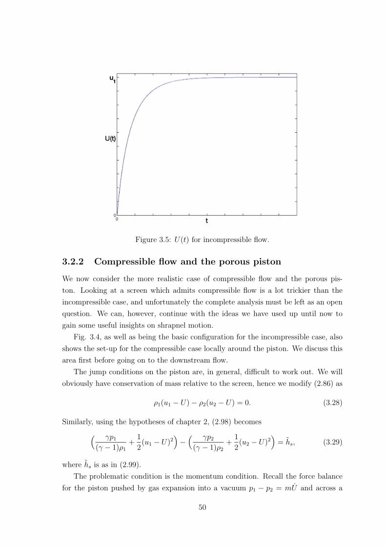
Figure 3.5: U(t) for incompressible flow.

3.2.2 Compressible flow and the porous piston

We now consider the more realistic case of compressible flow and the porous pis-

ton. Looking at a screen which admits compressible flow is a lot trickier than the

incompressible case, and unfortunately the complete analysis must be left as an open

question. We can, however, continue with the ideas we have used up until now to

gain some useful insights on shrapnel motion.

Fig. 3.4, as well as being the basic configuration for the incompressible case, also

shows the set-up for the compressible case locally around the piston. We discuss this

area first before going on to the downstream flow.

The jump conditions on the piston are, in general, difficult to work out. We will

obviously have conservation of mass relative to the screen, hence we modify (2.86) as

ρ1(u1 − U)− ρ2(u2 − U) = 0. (3.28)

Similarly, using the hypotheses of chapter 2, (2.98) becomes( γp1

(γ − 1)ρ1

+1

2(u1 − U)2

)−

( γp2

(γ − 1)ρ2

+1

2(u2 − U)2

)= hs, (3.29)

where hs is as in (2.99).

The problematic condition is the momentum condition. Recall the force balance

for the piston pushed by gas expansion into a vacuum p1 − p2 = mU and across a

50

shock was [p + ρ(u− U)2]21 = 0. In light of this, we might try a relationship of the

form

(p1 + µρ(u1 − U)2)− (p2 + µρ(u2 − U)2) = mU (3.30)

for a constant µ satisfying 0 ≤ µ ≤ 1. Here, µ would be a measure of how porous

the piston is. We see that µ = 0 would correspond to the piston expanding into a

vacuum, whereas µ = 1 would be equivalent to a shock wave (with a drag term).

Unfortunately, the use of such a factor cannot be justified by momentum balances.

Hence, we use the momentum balance given by

(p1 + ρ1(u1 − U)2)− (p2 + ρ2(u2 − U)2) = D + mU. (3.31)

We use the hypothesis [5] that the drag term will be written in terms of the square

of the downstream velocity and the downstream density for some drag coefficient Cd,

so

D =1

2ρ2Cd(u2 − U)2. (3.32)

Thus we have our jump conditions across the piston.

Before looking at the downstream motion, it is of importance to look at the entropy

jump across the piston. In the case of a shock wave, we have already obtained an

expression for the entropy jump across the shock (2.69). We need to reinvestigate

this now we have the extra terms D, mU and hs in the jump conditions across the

piston and wish to find out their effect.

Using the notation ε = M21 − 1 (M1 is the Mach number relative to the screen)

and introducing the nondimensional parameter

ξ =(mU + D − (γ − 1)hsρ2

p1

), (3.33)

we can mirror the analysis from before and manipulate Rankine-Hugoniot relations

to obtain the ratios p2

p1and ρ1

ρ2. For small ξ, rearrangement of (3.28), (3.29) and (3.31)

give lead to (p2

p1

)(ρ1

ρ2

)γ

∼ 1 + O(ξ). (3.34)

Hence the entropy jump will be O(ξ) for ξ sufficiently small. Obviously, if ξ ∼ ε3

(or smaller), then the entropy jump is what it was with no drag (D), loss (hs) or

acceleration term (mU), namely O(ε3).

For larger values of ξ, we can see that ξ will dominate the entropy jump, which

will be an important consideration in modelling the gas flow behind the screen. This

now leads us on to discussing possible downstream flow regimes.

51

Figure 3.6: A porous piston (screen) with barrel shocks.

Fig. 3.6 shows what we expect will happen after a short time. Choking can occur

in the screen, causing the flow to go from subsonic to supersonic. We then suppose

that barrel shocks (as in section 2.2.8) will form. These are shock waves formed

locally around the exit points of the screen. The geometry of these barrel shocks

is not known exactly, presenting us immediately with huge difficulties. As well as

having jump conditions across the porous piston, we will have jump conditions across

the barrel shocks. These are nontrivial.

The large time behaviour of the shocks is likely to be very different. We expect the

barrels to merge, leading to an arrangement as in Fig. 3.7. The flow here is divided

Figure 3.7: A porous piston (screen) with a shock to the right.

into three distinct regions. The first two regions are as discussed above, where the

gas rushes through the piston into region 2 and causes the piston to move with high

velocity. There will be a shock further downstream, which divides regions 2 and 3.

52

Rankine-Hugoniot shock conditions ((2.56), (2.57) and (2.58)) can be applied at

the boundary between 2 and 3, giving us three relationships between our gasdynamic

variables in the usual manner. To attempt to solve the system, we would try to solve

(3.31) for the piston with the jump conditions and shock conditions. We know that

there is a jump in entropy across the porous piston. This means that we cannot

use the Riemann invariants from (1) in region (2), as we unfortunately do not have

homentropic flow. What we do have is unknowns and equations relating them. We

cannot, however, solve the equations in region (2) analytically. Essentially, all we

have is boundary conditions at both boundaries of region (2) (from the shock jump

conditions and from the piston jump conditions) to accompany the general equations

of gasdynamics which hold in (2). These would have to be solved computationally.

In summary, we have developed a model for compressible gas flow through a move-

able screen. We have jump conditions (3.28), (3.29) and (3.31) which relate pressures,

densities and gas velocities either side of the piston. The drag coefficient Cd and K

need to be found experimentally. Downstream, we have shock waves which, in the

simplest case, will be as in Fig. 3.7. For this case, we can solve computationally using

Rankine-Hugoniot conditions across the shock (2.56), (2.57) and (2.58). Realistically,

we will have a more complicated shock-structure downstream.

3.3 Rock blasting theory

Our previous models consider gas flowing through thin layers of shrapnel, and hence

would be best applied to thin casings. The following model is on cliff blasting. It will

become clear that the theory developed applies more to thicker casings.

The processes involved in rock blasting are important in the mining industry. This

has motivated applied mathematicians to look at the problem and try and predict

the location of the rocks after blasting so that machinery can extract the ore with

the utmost efficiency. The mathematics involved is different to the theory we have

been looking at so far, though we can hopefully justify applying it to the shrapnel

problem. Here we look at an existing paper [20] which looks at the processes involved

when blasting a cliff.

3.3.1 Cliff Blasting

Before blasting takes place, the cliff must be prepared by drilling an array of vertical

boreholes in the cliff. These boreholes will normally stretch at least half of the cliff

height. The explosive charges are placed in the boreholes, which are then covered

53

with loose rocks. We are now ready to detonate the explosive in some prearranged

sequence.

The first thing that happens after the charge burns rapidly is that elastic waves

will propagate from the borehole into cliff, causing fracturing to take place. Fig. 3.8

shows this process, although in practice the wave will reflect off fractures and internal

cliff inhomogeneities and hence will not necessarily be strictly vertical as shown. Also,

depending on the borehole, we will get propagation into terra firma (the solid rock

which won’t be cracked), though reflections from this will be neglected in the following

model. This stage lasts about 10 milliseconds, and, depending on the size of the cliff,

all an observer would see from this stage would be the cliff vibrate.

Figure 3.8: Elastic/plastic wave propagation leading to fracturing.

The next thing an observer would see is puffs of smoke (or dust) emerging from

the external boundaries of the cliff. The high pressure gas caused by the burning of

the charge has propagated through the cliff to cause this. In doing so, the gas links up

some of the existing fractures and may create additional fractures. We might expect

the fully fractured rocks to start accelerating at this stage, but this does not happen

as they are held securely in place by the rock which the gas has not reached yet. This

stage will last in the order of 100 milliseconds.

54

The rock is now ready to move. This will occur when the cliff cannot hold the

high pressure gas. The build up of pressure in the cliff is relieved as the completely

fractured rock is rapidly accelerated and will begin to move, as shown in Fig. 3.9.

The red line shows the movement of the front where rock acceleration starts to take

place. This rock acceleration will take in the order of 10 milliseconds.

Figure 3.9: Rocks from the fully fractured cliff start to move, starting from the right-hand face.

Finally, the rocks which are now in motion will free-fall under gravity. They will

form a “muck-pile”, allowing valuable ore to be obtained with relative ease. The

free-fall section will last the order of one second.

3.3.2 Existing model

An existing model [20] analyses the high pressure gas propagation and the build up

of pressure leading to rock movement in a cliff. The model uses the idea of two-phase

flow, which, as the name suggests, refers to there being two phases of a substance in

a flow. Two-phase flow typically involves the phases being liquid and gas, though in

the cliff blasting case, the different phases are the gas and the rock. Often, the flow

is turbulent which leads to some kind of averaging being essential to model the mean

flow [11]. We do not average as such here, though need to introduce a new variable

α, the void fraction which is the gas volume fraction.

55

To set up the two-phase flow model, we first need to make some assumptions

about the cliff and gas. Firstly, the cliff is assumed to be homogeneous. We also need

to assume that the rocks aren’t porous, and that the gas flow is limited to the cracks

between the rocks only. This assumption is quite a large one, as many rocks tend to

be very porous, which would have consequences on the gas propagation. It is also

assumed that no cracking occurs in this stage and that the distribution of the cracks

is known from the earlier stage.

Hence the basic equations of motion come from conservation of mass and momen-

tum for the rock and for the gas. Mass conservation gives

Dg

Dt(αρg) + αρg∇.v = 0 (3.35)

Dr

Dt((1− α)ρr) + (1− α)ρr∇.u = 0 (3.36)

where subscripts g and r refer to the gas and rock respectively, v and u are the gas

and rock velocities (respectively), α is the volume fraction of gas and DDt

denotes the

material derivative for the respective phase.

Neglecting any drag between the phases and assuming that the pressure is the

same in both phases, we can similarly use conservation of momentum to obtain

ρgαDvDt

+ α∇p = 0 (3.37)

ρr(1− α)DuDt

+ (1− α)∇p = 0. (3.38)

An important nondimensional parameter is given by

β =Kp0ρr0

ρ0

(3.39)

where K is proportional to the Young’s Modulus of the rock, ρr0 the initial rock

density, ρ0 the initial gas density in the borehole and p0 the initial pressure in the

borehole. The Young’s modulus is a measure of the stiffness of the material (rock

in our case) as a function of its density. Kp0 will be used as a suitable scale for the

void fraction. Typically, for rocks, β has a value of the order 0.01 and the Young’s

modulus for rocks is of the order 107Pa.

Assuming the gas is ideal, we will have pp0

= ( ρρ0

)γ. Nondimensionalisation of the

equations will give us a hyperbolic system for the motion of the gas and rock. In

choosing appropriate scales for nondimensionalisation, we will have different choices

56

to make depending on whether we are dealing with the stage where the rocks are free

to move or not.

The more interesting stage for us will involve the rocks being free to move. Looking

at one-dimensional equations we arrive at, taking the limit as β → 0,

∂ρ

∂t+ a(ρ)

∂u

∂x= 0 (3.40)

∂u

∂t+ b(ρ)

∂ρ

∂x= 0 (3.41)

where a(ρ) = (γργ−1 + 1ρ2 )

−1 and b(ρ) = γργ−1.

Figure 3.10: Cliff considered as a 2D model.

To solve this hyperbolic system, we need to impose some initial conditions. We

make the following simplifications to the problem in order to enable us so obtain an

analytic solution. Firstly, we assume that the cliff area is square, and that two sides

of the square will be external surfaces (Fig. 3.10). We also assume that gas pressure

and void fraction are initially spatially uniform, so we have the boundary condition

57

α(x, 0) = 1 = ρ(x, 0). For simplicity, the inhomogeneity owing to the borehole is

neglected.

The boundary condition used is that the pressure on the external surfaces of the

cliff is atmospheric pressure (patmos), say

p = patmos/p0 = εγ (3.42)

and that the boundaries by terra firma have u.n = 0 (noting that p is nondimensional

in (3.42)).

Substituting ρ = g(s(x, t)) and choosing dgds

=(

a(g)b(g)

) 12

we can obtain the Riemann

invariants of the system via( ∂

∂t± (ab)

12

∂

∂x

)(u± s) = 0. (3.43)

Hence we have simple wave flow (section 2.2.5) as u± s = constant on dxdt

= ±(ab)12

and so using the initial conditions on α and ρ, we obtain the a characteristic diagram

(Fig. 3.11) which leads to an analytical solution:

Figure 3.11: Characteristic diagram for cliff fracturing.

ρ =

ε −(

γεγ+1

γεγ+1+1

) 12

< xt

< 0 (1)((x

t)2

γ(1−(xt)2)

) 1γ+1 −

(γ

γ+1

) 12

< xt

< −(

γεγ+1

γεγ+1+1

) 12

(2)(3.44)

58

and

u =

∫ 1

ρ

zγ−3

2 (γ2zγ+1 + γ)12 dz (3.45)

Reflections off the face x = −1 have been neglected. Hence this solution is only

valid until information from the face at x = 0 has reached x = −1, at time t = tc.

For γ = 1, we can calculate the integral and get that u ∼ log ε + O(1) as ε → 0

We can also calculate the velocity at the edge of the cliff by substituting ρ = ε into

(3.45).

Looking at plots (Fig. 3.12) of the void fraction and rock velocity for different

times, we observe that the rocks on the outermost layer of the cliff fly off with a very

high velocity (almost like a boundary layer), whereas those nearer to x = −1 won’t

fly off until a later time. This is what we expect physically, and indeed it is what is

seen.

Figure 3.12: Graphs showing void fraction (scaled) and rock speed (scaled), as func-tions of position for different values of time. The blue line indicates the smallest timevalue, then working up to the olive line. γ is taken to be 1.3.

59

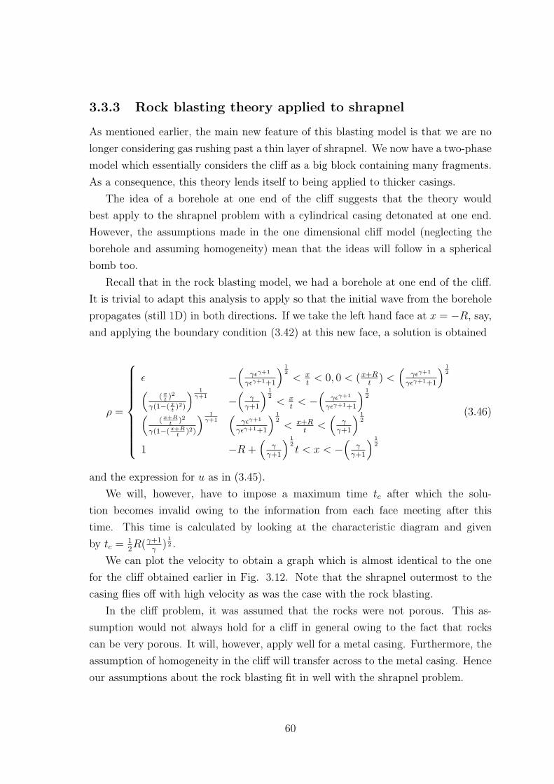
3.3.3 Rock blasting theory applied to shrapnel

As mentioned earlier, the main new feature of this blasting model is that we are no

longer considering gas rushing past a thin layer of shrapnel. We now have a two-phase

model which essentially considers the cliff as a big block containing many fragments.

As a consequence, this theory lends itself to being applied to thicker casings.

The idea of a borehole at one end of the cliff suggests that the theory would

best apply to the shrapnel problem with a cylindrical casing detonated at one end.

However, the assumptions made in the one dimensional cliff model (neglecting the

borehole and assuming homogeneity) mean that the ideas will follow in a spherical

bomb too.

Recall that in the rock blasting model, we had a borehole at one end of the cliff.

It is trivial to adapt this analysis to apply so that the initial wave from the borehole

propagates (still 1D) in both directions. If we take the left hand face at x = −R, say,

and applying the boundary condition (3.42) at this new face, a solution is obtained

ρ =

ε −(

γεγ+1

γεγ+1+1

) 12

< xt

< 0, 0 < (x+Rt

) <(

γεγ+1

γεγ+1+1

) 12(

(xt)2

γ(1−(xt)2)

) 1γ+1 −

(γ

γ+1

) 12

< xt

< −(

γεγ+1

γεγ+1+1

) 12(

(x+Rt

)2

γ(1−(x+Rt

)2)

) 1γ+1

(γεγ+1

γεγ+1+1

) 12

< x+Rt

<(

γγ+1

) 12

1 −R +(

γγ+1

) 12t < x < −

(γ

γ+1

) 12

(3.46)

and the expression for u as in (3.45).

We will, however, have to impose a maximum time tc after which the solu-

tion becomes invalid owing to the information from each face meeting after this

time. This time is calculated by looking at the characteristic diagram and given

by tc = 12R(γ+1

γ)

12 .

We can plot the velocity to obtain a graph which is almost identical to the one

for the cliff obtained earlier in Fig. 3.12. Note that the shrapnel outermost to the

casing flies off with high velocity as was the case with the rock blasting.

In the cliff problem, it was assumed that the rocks were not porous. This as-

sumption would not always hold for a cliff in general owing to the fact that rocks

can be very porous. It will, however, apply well for a metal casing. Furthermore, the

assumption of homogeneity in the cliff will transfer across to the metal casing. Hence

our assumptions about the rock blasting fit in well with the shrapnel problem.

60

Figure 3.13: A snapshot of shrapnel velocity for a two-faced cliff with R = 1.

The physical properties of the casing and charge need to be such that β (3.39) is

small. Recall that β is proportional to the Young’s modulus of the substance, which

was of the order 107Pa for rock. Tabulated values of Young’s moduli give a value of

1010Pa for aluminium (which is a typical casing material) and 1012 for steel. Thus the

solution can only be justifiably applied if, in the notation of (3.39),p0ρc0

ρ0is sufficiently

small, where ρc0 is the initial casing density.

Hence we can conclude, as long as we are justified in taking the limit β → 0,

that the shrapnel velocity will mirror that of the rock velocity as in Fig. 3.12. The

nondimensional parameters will change owing to the different nature of the material

involved, but the rock-blasting idea gives us a good idea of how the shrapnel velocity

will evolve through time.

61

3.4 Comparison of the models

The first models were all based on obtaining a solution for the shrapnel velocity

in 1-dimension. The models considered the gas flowing into or past a thin layer of

shrapnel.

Our initial idea was to model the shrapnel as a piston being pushed into a vacuum

by expanding gas (section 3.1). This is quite a basic model and overestimates the

piston velocity as the model does not allow for any seepage and neglects any resistance

we would have acting against the piston (as we modelled it as expanding into a

vacuum). Although the model is an approximation of shrapnel motion, it nevertheless

gives an idea of the expected motion. It provides us with an indication that there

will be a maximum velocity for the shrapnel, which is intuitively obvious, as the we

don’t expect the shrapnel velocity to exceed the gas velocity.

We then modelled the shrapnel as a contact discontinuity in a shock tube (section

2.2.6). This is another simple model. It, like the previous model, does not allow

seepage through the discontinuity. Furthermore, it does not account for the mass of

the shrapnel and so predicts a constant velocity for the shrapnel which depends on

the values that p and ρ take in different regions, as demonstrated in section 2.2.6.

The aim of these basic models was to give a grounding for a model which allows

gas seepage through gaps between fragments. This gave us the motivation for flow

past a porous piston, in which we modelled the shrapnel fragments as a screen. For

simplicity, incompressible flow was considered first (section 3.2.1). Jump conditions

established in chapter 2 enable us to solve for the piston velocity analytically. As

with our first model, the solution to this model indicates that the shrapnel tends to

a constant velocity as t→∞, which, in this case, is the upstream gas velocity. This

model is not, however, entirely realistic. This motivated the porous piston problem

being modelled with compressible gas flow.

The compressible gas flow into the porous piston is the most realistic model (sec-

tion 3.2.2). It is, however, also more intricate and complicated owing to the admission

of shock waves. We derived a condition on the entropy jump across the piston, and

showed that it is very much dependent on the drag. This affects the flow behind the

porous piston (screen). We have suggested possible ideas for flow behind the screen

we have to conclude that, as we do not have homentropic flow, it is nontrivial to solve

for the shrapnel velocity analytically. The possibility of choked flow makes it even

more difficult to put forward a soluble model as we will have to predict the nature of

the downstream shock waves. However, if we make the assumption of a normal shock

62

as in Fig. 3.7, the model can be solved computationally. Hence, although this model

is the most realistic, it is the also the most difficult to solve.

Our final model was based on cliff-blasting theory (section 3.3.2). This uses a

different approach entirely. In particular, we are no longer considering gas flow past

a thin layer of metal, but are considering a large section of material which consists

of shrapnel and gas (equivalent to the cliff). The mathematics behind the model

need certain physical assumptions about the casing to be made in order to apply the

model. Assuming these assumptions are justified, the model predicts the shrapnel

will fly off with high velocity from the edge of the casing, as expected. Plots of the

velocity of the rock (shrapnel) as a function of position for different values of time t

demonstrate this (Fig. 3.12). Hence, this model gives us some insight into shrapnel

motion which the other models did not.

63

Chapter 4

Conclusions

4.1 Summary of work

The motivation for this problem was to develop models for shrapnel motion for use

by QinetiQ. The background to the problem was described in chapter 1 where we

outlined the general processes involved. We reinforced these ideas with experimental

evidence.

We then split chapter 2 up into two parts; incompressible and compressible flow.

Our aim in this chapter was to give sufficient background material to enable us to

develop 1-dimensional models for shrapnel motion. Firstly, we considered background

material on incompressible flows. The differences between laminar and turbulent

flow were highlighted, leading to the discussion of jump conditions and conservation

laws. The section on incompressible flow culminated in the concept of head losses

and different loss coefficients for various flow geometries. We then established a

background on compressible flow. We used some of the ideas from incompressible

flow and looked in particular at choking for different pipe geometries.

In chapter 3, we used ideas from incompressible and compressible flows to develop

several models for shrapnel motion. The first models were quite basic, motivating

the more sophisticated later models. An alternative model which used a different

approach was discussed, before bringing all the ideas together in a comparison of the

models.

4.2 Further work

This dissertation has made a start on investigating shrapnel motion. Some of the

points raised merit further investigation. In chapter 2, we discussed loss coefficients

in some detail for incompressible flow. We were not, however, able to complete the

64

same analysis for compressible flow and determine loss coefficients for various pipe

geometries. This needs to be looked at in more detail. A more detailed investigation

of drag coefficients will also be useful. These could then be utilised in the porous

piston models in both the incompressible and compressible cases.

There are also many new avenues that can be explored. Firstly, most of our

modelling has been in a 1-dimensional geometry. Although this has given insight into

the problem, it would be beneficial to look at casing with a spherical geometry. We

would need a discussion on spherical shock waves and could perhaps look at blast

waves, in which we would model the explosion as a sudden release of energy at the

centre of the bomb at time t = 0.

The screen model, although it can accommodate different sized elements in the

screen (by means of the solidity) does not allow different pieces of shrapnel in the

screen to have an individual acceleration, as all the elements of the screen move

together as a single body. This motivates work on modelling different sizes of fragment

with different accelerations, as in reality, the fragments are likely to vary in size.

Another new idea would be to develop a better two-phase model (gas and shrapnel)

comparing the shrapnel to, say, so-called dusty gas flow [15].

4.3 Final comments

We have suggested possible improvements for models to the shrapnel problem. It is

likely that further experimental evidence will lead to new insight into the problem,

and may reinforce some of the models developed in this dissertation. We have built

the foundations to the problem which should go some way into developing a more

complete model describing shrapnel motion.

65

Bibliography

[1] http://www.chicagohs.org/hadc/visuals/artifact/015A14A.htm.

[2] D.J. Acheson. Elementary fluid dynamics. Oxford University Press, 1998.

[3] S.T.S. Al-Hassani, H.G. Hopkins, and W. Johnson. A note on the frag-

mentation of tubular bombs. Int. J. Mech. Sci., 11:545–549, 1969.

[4] C.E. Anderson, W.W. Predebon, and R.R. Karpp. Computational mod-

eling of explosive-filled cylinders. Int. J. Engng Sci., 23:1317–1331, 1985.

[5] R.P. Benedict. Fundamentals of pipe flow. John Wiley & Sons, 1980.

[6] W.T. Bernardi, J.H. Linehan, and L.H. Hamilton. Low Reynolds num-

ber loss coefficient for fine mesh screens. Trans. ASME J. Fluids Eng., 98:763–

764, 1976.

[7] M. D. Blackford. Casing mechanics. MSc Dissertation, Oxford University,

2001.

[8] W.G. Cornell. Losses in flow normal to plane screens. Trans. ASME., 80:791–

799, 1958.

[9] R. Courant and K.O. Friedrichs. Supersonic flow and shock waves.

Springer-Verlag, 1948.

[10] M.M. Denn. Process fluid mechanics. Prentice-Hall, 1980.

[11] A.C. Fowler. Mathematical Models in the Applied Sciences. Cambridge Uni-

versity Press, 1998.

[12] C.R. Hoggatt and R.F. Recht. Fracture behavior of tubular bombs. J.

Appl. Phys., 39:1856–1862, 1968.

66

[13] J.E.A. John and W.L. Haberman. Introduction to fluid mechanics. Prentice-

Hall, 1988.

[14] H. W. Leipmann and A. Roshko. Elements of gasdynamics. John Wiley &

Sons, 1956.

[15] F.E. Marble. Dynamics of dusty gases. Ann. Rev. Fluid Mech., 2:397–446,

1970.

[16] D.S. Miller. Internal flow systems. BHRA Group (Information Services),

1990.

[17] Y. Nakayama and R.F. Boucher. Introduction to fluid mechanics. Arnold,

1999.

[18] H. Ockendon and J. R. Ockendon. Viscous flow. Cambridge University

Press, 1995.

[19] H. Ockendon and A.B. Tayler. Inviscid fluid flows. Springer-Verlag, 1983.

[20] C.P. Please, A.A. Wheeler, and P. Wilmott. A mathematical model of

cliff blasting. SIAM J. Appl. Math., 1:117–127, 1987.

[21] J.A. Smits. A physical introduction to fluid mechanics. John Wiley & Sons,

2000.

[22] G. I. Taylor. The fragmentation of tubular bombs. Fluids of Mechanics,

Scientific Papers of G. I. Taylor, 2:387–390, 1944.

[23] G.I. Taylor. Analysis of the explosion of a long cylindrical bomb detonated

at one end. Mechanics of Fluids, Scientific Papers of G. I. Taylor, 2:277–286,

1941.

[24] S. Whitaker. Introduction to fluid mechanics. Prentice-Hall, 1968.

67