Short-term Stock Market Price Trend Prediction Using a ...
128
Short-term Stock Market Price Trend Prediction Using a Customized Deep Learning System by Jingyi Shen A thesis submitted to the Faculty of Graduate and Postdoctoral Affairs in partial fulfillment of the requirements for the degree of Master of Information Technology in Information Technology (Digital Media) Carleton University Ottawa, Ontario © 2019, Jingyi Shen
Transcript of Short-term Stock Market Price Trend Prediction Using a ...

Short-term Stock Market Price Trend Prediction Using a
Customized Deep Learning System
by
Jingyi Shen
A thesis submitted to the Faculty of Graduate and Postdoctoral
Affairs in partial fulfillment of the requirements for the degree of
Master of Information Technology
in
Information Technology (Digital Media)
Carleton University
Ottawa, Ontario
© 2019, Jingyi Shen

ii
Abstract
In big data era, deep learning solution for predicting stock market price trend becomes
popular. We collected two years of Chinese stock market data according to the financial
domain, proposed a fine-tuned stock market price trend prediction system with
developing a web application as the use case, meanwhile, conducted a comprehensive
evaluation on most frequently used machine learning models and concludes that our
proposed solution outperforms leading models. The system achieves an overall trend
predicting accuracy of 93%, also achieves significant high scores in other machine
learning metrics score in the meantime. Thus, this work provides a solid foundation for
further price prediction by classifying the price trend accurately. With the detail-designed
evaluation on prediction term lengths, feature engineering and data pre-processing
methods, this work also contributes to the stock analysis research community in both
financial and technical domain.

iii
Acknowledgements
I want to extend thanks to many people, all over the world, who so generously helped me
during my Master’s degree and contributed to this thesis work.
Special mention goes to my supervisors, Dr. Omair Shafiq. During my Master’s degree,
Dr. Shafiq has always been providing his tremendous academic support. He is
enthusiastic in academic, and his attitude encourages me a lot as a researcher working in
data science. He also generously provided me funding help to support my trip to
CBDCom2019 in Japan, which is the first time I present at an international conference.
I would also like to express my very profound gratitude to Dr. Anthony Whitehead, who
was supposed to be my supervisor but unfortunately passed away before I entered
Carleton University. Without Dr. Whitehead, I would never get the opportunity to study
in Canada. Thanks for giving me the chance to become a student in CLUE; it is not about
the funding support only, but also the precious internship opportunity to work in You. i
TV.
I am also hugely appreciative to Dr. Audrey Girouard, the director of CLUE, who has
provided me countless opportunities to participate in the HCI activities, and inspired me
to exploit deep learning technique to contribute to UX research domain.
Also, profound gratitude goes to, Dr. Olga Baysal, Dr. Frank Dehne. Thanks for
introducing me to the world of big data, and always being patient when I asked the
fundamental questions.
Last but not least, thanks to my family and friends, especially my mom. Thanks for
supporting me to complete my Master’s degree abroad. This thesis work will never exist

iv
without her, not only the financial and mental support, but also her passion in the stock
market. I wish my thesis work can help her as a return, even a little. Thanks to all her
generous support given to me all the time.
v
Table of Contents
Abstract ................................................................................................................................................... ii
Acknowledgements ................................................................................................................................. iii
List of Tables .......................................................................................................................................... vii
List of Illustrations................................................................................................................................. viii
Chapter 1: Introduction ........................................................................................................................... 1
Chapter 2: Dataset of Chinese Stock Market ........................................................................................... 6
2.1 Introduction of Dataset Preparation ................................................................................................. 6
2.2 Survey of Existing Works in Financial Domain .................................................................................. 6
2.3 Description of Our Dataset .............................................................................................................. 15 2.3.1 Data Structure ....................................................................................................................... 15 2.3.2 Basic Data .............................................................................................................................. 19 2.3.3 Trading Data .......................................................................................................................... 25 2.3.4 Finance Data .......................................................................................................................... 28 2.3.5 Other Reference Data ............................................................................................................ 28
2.4 Research Opportunity ..................................................................................................................... 34
Chapter 3: Survey of Related works ...................................................................................................... 35
3.1 Technical Related Works ................................................................................................................. 35
3.2 Comparative Analysis ...................................................................................................................... 54
3.3 Gap Analysis .................................................................................................................................... 55
Chapter 4: Design of Proposed Solution ................................................................................................ 58
4.1 Problem Statement ......................................................................................................................... 58 4.1.1 RQ1: How does feature engineering benefit model prediction accuracy? ....... 58 4.1.2 RQ2: How do findings from financial domain benefit prediction model design? ................. 58 4.1.3 RQ3: What is the best algorithm for predicting short-term price trend? ............................. 59
4.2 Technical Background – Technical Indices ...................................................................................... 61
4.3 Proposed Solution ........................................................................................................................... 64
4.4 Detailed Technical Design Elaboration ............................................................................................ 67 4.4.1 Feature Extension .................................................................................................................. 68 4.4.2 Recursive Feature Elimination ............................................................................................... 70 4.4.3 Principal Component Analysis ............................................................................................... 70 4.4.4 Long Short-Term Memory ..................................................................................................... 71
4.5 Design Discussion ............................................................................................................................ 72
4.6 Algorithm Elaboration ..................................................................................................................... 73 4.6.1 Algorithm 1: Short-term Stock Market Price Trend Prediction - Hybrid Feature Engineering Using FE+RFE+PCA ............................................................................................................................... 74
vi
4.6.2 Algorithm 2: Price Trend Prediction Model Using LSTM ....................................................... 79
4.7 Use Case of Proposed Solution ........................................................................................................ 81 4.7.1 Related Applications .............................................................................................................. 82 4.7.2 Application Deployment and GUI Explanation ...................................................................... 83 4.7.3 Potential of the Use Case ...................................................................................................... 84
Chapter 5: Evaluation ............................................................................................................................ 86
5.1 Term Length .................................................................................................................................... 87
5.2 Feature Extension and RFE .............................................................................................................. 90
5.3 Feature Reduction Using Principal Component Analysis ................................................................. 92
5.4 Model Performance Comparison .................................................................................................... 96 5.4.1 Comparison with Related Works ........................................................................................... 97 5.4.2 Proposed Model Evaluation - PCA Effectiveness ................................................................. 102
5.5 Discussions and Implications ......................................................................................................... 103 5.5.1 RQ1: How does feature engineering benefit model prediction accuracy? ......................... 103 5.5.2 RQ2: How do findings from financial domain benefit prediction model design? ............... 103 5.5.3 RQ3: What is the best algorithm for predicting short-term price trend? ........................... 104 5.5.4 Complexity Analysis of Proposed Solution .......................................................................... 105 5.5.5 Other Findings ..................................................................................................................... 107
5.5.5.1 Choose a proper pre-processing method for the feature set .................................... 107 5.5.5.2 Term length significantly affects the price trend prediction result ........................... 107 5.5.5.3 How does PCA algorithm affect the model performance .......................................... 108 5.5.5.4 Lower rate of TN than TP ........................................................................................... 109
Chapter 6: Future Work ....................................................................................................................... 110
Chapter 7: Conclusion ......................................................................................................................... 111
References ........................................................................................................................................... 113
vii
List of Tables
This is the List of Tables.
Table 1 Basic Data ............................................................................................................ 20
Table 2 Stock List Data..................................................................................................... 21
Table 3 Trading Calendar ................................................................................................. 22
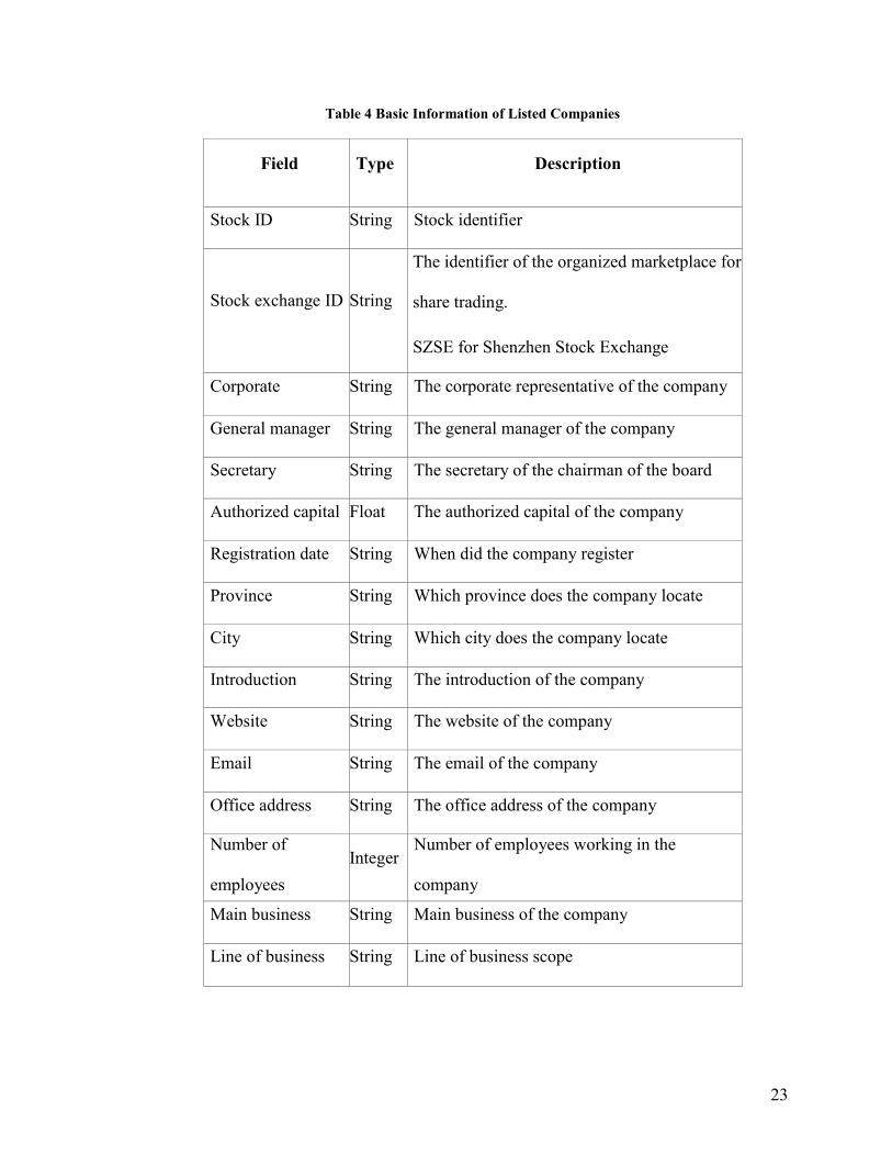
Table 4 Basic Information of Listed Companies .............................................................. 23
Table 5 Rename History ................................................................................................... 24
Table 6 List of Constituent Stocks .................................................................................... 24
Table 7 Daily Trading Data .............................................................................................. 25
Table 8 Fundamental Data ................................................................................................ 26
Table 9 Financial Report Disclosure Date ........................................................................ 28
Table 10 Top 10 Shareholders Data .................................................................................. 29
Table 11 Top 10 Floating Shareholders Data ................................................................... 30
Table 12 Daily Top Trading List by Institution ................................................................ 30
Table 13 Daily Top Transaction Detail ............................................................................ 31
Table 14 Block Trade Transaction Data ........................................................................... 32
Table 15 Public Fund Positioning Data ............................................................................ 33
Table 16 Comparative Analysis Table .............................................................................. 49
Table 17 Feature Extension Method Selection ................................................................. 69
Table 18 Effective Features Corresponding to Term Lengths .......................................... 89
Table 19 Relationship Between the Number of Principal Components and Training
Efficiency .......................................................................................................................... 93
Table 20 How Does the Number of Selected Features Affect the Prediction Accuracy .. 93
Table 21 Accuracy and Efficiency Analysis on Feature Pre-processing Procedures ....... 95
Table 22 Model Performance Comparison – Metric Scores ............................................. 98
Table 23 Comparison of Proposed Solution with Related Works .................................. 101
Table 24 Proposed Model Performance Comparison - With and Without PCA ............ 102
viii
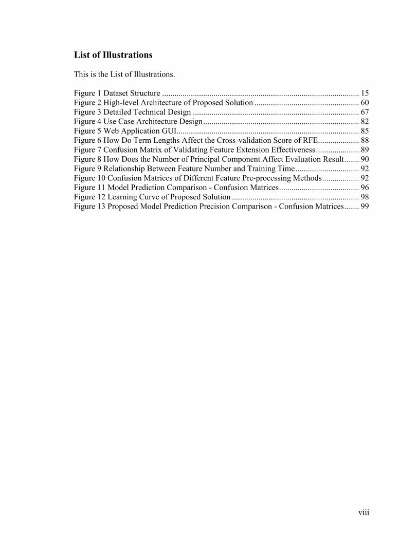
List of Illustrations
This is the List of Illustrations.
Figure 1 Dataset Structure ................................................................................................ 15
Figure 2 High-level Architecture of Proposed Solution ................................................... 60
Figure 3 Detailed Technical Design ................................................................................. 67
Figure 4 Use Case Architecture Design ............................................................................ 82
Figure 5 Web Application GUI......................................................................................... 85
Figure 6 How Do Term Lengths Affect the Cross-validation Score of RFE.................... 88
Figure 7 Confusion Matrix of Validating Feature Extension Effectiveness ..................... 89
Figure 8 How Does the Number of Principal Component Affect Evaluation Result ....... 90
Figure 9 Relationship Between Feature Number and Training Time ............................... 92
Figure 10 Confusion Matrices of Different Feature Pre-processing Methods .................. 92
Figure 11 Model Prediction Comparison - Confusion Matrices ....................................... 96
Figure 12 Learning Curve of Proposed Solution .............................................................. 98
Figure 13 Proposed Model Prediction Precision Comparison - Confusion Matrices ....... 99

1
Chapter 1: Introduction
Stock market is one of the major fields that investors dedicated to, thus stock market
price trend prediction is always a hot topic for researchers from both financial and
technical domain. While during our literature review, we found merely a limited overlap
in previous research from these two domains. In this research project, our objective is to
build a state-of-art prediction model for price trend prediction, which focuses on short-
term.
As concluded by Fama in (Malkiel & Fama, 1970), financial time series prediction is
known as a notoriously difficult task due to the generally accepted, semi-strong form of
market efficiency and the high level of noise. Back to the year 2003, Wang et al. in
(Wang & Lin, n.d.) already applied Artificial Neural Network on stock market price
prediction and focused on volume, a specific feature of the stock market, leveraged
research. One of the key findings is that the volume is not effective in improving the
forecasting performance on the datasets they used, which was S&P 500 and DJI. Ince and
Trafalis in (Ince & Trafalis, 2008) targeted to short-term forecasting and applied their
support vector machine (SVM) model on stock price prediction. Their main contribution
is performing a comparison between multi-layer perceptron (MLP) and SVM then found
that most of the scenarios SVM outperforms MLP, while the result is also affected by
different trading strategies. In the meantime, researchers from financial domains were
applying conventional statistical methods and signal processing techniques on analyzing
stock market data. Lee in (H. S. Lee & Lee, 2006) performed a wavelet analysis focusing
on international transmission of stock market movement. The related works in Chapter
2
2.2 were using the similar conventional statistical methods to analyze the specific
phenomena, which narrows down the usage of their proposed solution. Compared with
artificial intelligence approaches, the conventional statistical methods seem to be a lack
of generalization.
The optimization techniques such as principal component analysis (PCA) were also
applied in short-term stock price prediction (Lin, Yang, & Song, 2009). During the years,
researchers are not only focusing on stock price-related analysis, but also trying to
analyze stock market transactions such as volume burst risks, which expands the stock
market analysis research domain broader and indicates this research domain still has high
potential (Shih, 2019). As the artificial intelligence technique boosting in recent years,
many proposed solutions are trying to collaborate the machine learning and deep learning
approaches based on previous approaches, then propose new metrics serve as training
features such as (G. Liu & Wang, 2019). This type of previous works belongs to feature
engineering domain and can be considered as the inspiration of feature extension idea.
Liu et al. in (S. Liu, Zhang, & B, 2017) proposed a convolutional neural network (CNN)
and long short-term memory (LSTM) neural network model to analyze the quantitative
strategy in stock markets. The CNN serves for the stock selection strategy, automatically
extracts features based on quantitative data, then follows an LSTM to preserve the time-
series features for improving the profits. The latest work also proposes a similar hybrid
neural network architecture, integrates a convolutional neural network with a
bidirectional long short-term memory to predict stock market index (Eapen, Automation,
& Market, 2019). While the symptom of researchers frequently propose fancy neural

3
network solution architectures also brings further discussion about the topic: if the high
training consumption is worth the result.
In this research project, we used a dataset built and formed by ourselves. The data source
is an open-sourced data API called Tushare (“Tushare API,” 2018), we illustrate the data
collection details in Chapter 2.3.
We obtain price data of 3558 stocks from Chinese stock market; the date range is from
Jan 2017 to Mar 2019. We choose the stocks by eliminating the listing date, only choose
the stocks whose listing dates are between this date range. The data of year 2017 and
year 2018 are for training purpose; then we build the testing dataset by using the first-
season price data of 2019.
All the models are used CPU-based training procedure.
Based on an abundant previous works review, we come up with three major research
questions and propose a comprehensive solution followed by a thorough evaluation
which aims to resolve the research questions. The first objective for this research is to
explore how feature engineering benefits model prediction accuracy. By reviewing the
related works in both financial and technical domains, we raise the second objective to
convert findings from financial domain to the technical procedure that can benefit
prediction model design. The third major purpose of this paper is to research how
different machine learning algorithms perform on short-term price trend prediction.
In respect of building an efficient model to resolve a specific term length of price trend
prediction problems, we make below contributions.
· First, we demonstrate an effective method to convert the findings from the
financial domain to a technical procedure consequently contributes to the model
4
prediction evaluation metric scores. We name this method as feature extension and
exploit three means of data pre-processing. The evaluation result has proved that our
proposed feature extension is significantly helpful to feature engineering procedures.
· Second, we focus on short-term stock market price trend prediction and
customized a state-of-the-art deep learning system using Long Short-term Memory
(LSTM). Our approach can accurately select the most effective features by RFE
algorithms. By exploiting PCA procedure, it can also achieve a great promotion in model
training efficiency without sacrificing too much accuracy. Meanwhile, we involve a state-
of-the-art Long Short-term Memory (LSTM) model to retain the features’ time
dependency and achieves 96%, a significantly high accuracy in predicting price-up trend
and a 93.25% overall prediction accuracy.
· Third, by performing a comprehensive evaluation on models used by the most
related works and each component of our proposed system, we conclude varies findings
which worth leveraging a more in-depth research. It contributes to both technical and
financial domain related to stock market analysis by providing new research questions on
the perspectives of feature engineering, term lengths, and data pre-processing methods.
Besides, other contributions would be the Chinese stock market dataset we collected and
the use case based on our proposed solution.
The novelty of our proposed solution causes our work distinct from previous proposed
solution is that we proposed a fine-tuned system instead of an LSTM model only. We
observe from previous works and find the gaps between investors and researchers who
dedicate in technical domain, and proposed a solution architecture with a comprehensive
feature engineering procedure before training the prediction model. With the success of

5
feature extension method collaborate with recursive feature elimination algorithms,
almost all the machine learning algorithms can achieve high accuracy scores (around
90%) of short-term price trend prediction. It proved the effectiveness of our proposed
feature extension as a novel method of feature engineering. While after introducing the
customized LSTM model, we further improved the prediction scores in all evaluation
metrics and outperformed the machine learning models in similar previous works.
The remainder of this paper is organized as follows. Chapter 3 explains the technical
keywords that frequently appear in this paper, stresses the strengths and weaknesses of
related works, and describes how the previous works related to our research project. We
have also concluded a table for quick indexing related works in Chapter 3.2. This chapter
also provides the technical background by detailed illustrating the technical indices we
exploit in this paper. Chapter 4 is the methodology part; it covers the gap analysis,
research problems, and proposed solution. Detailed technical design with algorithms and
how the model implemented are also included in this section. At the end of this chapter it
also illustrates the use case of our proposed solution, a flexible and easy-to-access web
application designed for individual investors. Chapter 5 presents the comprehensive
evaluation of our proposed model not only by comparing with the models used in most
related works but also in the optimization aspect. Then follows by a subsection, which
initials a discussion based on the findings to answer research questions, also other
valuable findings that worth bringing about. Chapter 6 lists further research directions
that are promising for this paper. Chapter 7 concludes.

6
Chapter 2: Dataset of Chinese Stock Market
2.1 Introduction of Dataset Preparation
This chapter is a detailed illustration of the dataset contribution.
The second section is the survey part. Stock market-related data are diverse, so we do a
comprehensive literature review of financial research works in stock market analysis to
specify the data collection directions.
After collecting the data based on the findings from a literature review of previous
research works, we define the data structure of the dataset. Section 2.3 described the
dataset in detail, it includes the data structure, and data tables in each category of data
with the segment definitions.
We also briefly introduce the potential research opportunities of this dataset in the fourth
section.
2.2 Survey of Existing Works in Financial Domain
In this part, we list the literature review data collection. The primary content for this part
is the literature review of previous works in financial domain; they provided the direction
of what kind of data we should collect, and how they will benefit the stock market
analysis.
We can regard data as raw oil that is being generated with every passing second
(Mohammad, Afshar, & Parul, 2018). Before researching the previous works in financial
domain for data collection instruction, we first go through the related works of existing
public datasets. This step helps us to design the structure of stock market data.

7
Following section explains two primary reasons of collecting two years Chinese stock
market from 2017 to 2018. First reason is that the stock market data of 2017 and 2018 are
the most recent data that we had access at the beginning of the research, instead of using
historical data, we prefer to use the latest data to keep the evaluation results of our
research project more convincing. Alvarez-Ramirez et al. in (Alvarez-Ramirez, Jose,
Alvarez, Rodriguez, & Fernandez-Anaya, 2008) used historical data but still analyzed the
emergence of anti-correlated behavior in recent two years. Second reason is that two
years is a very popular period length among financial data analysis, not only for investors
but also for researchers. Paranjape-Voditel and Deshpande in (Paranjape-Voditel, Preeti,
& Deshpande, 2013) took the period of investment as two years, and mentioned that two-
year is a reasonable period because this period can be easily extended but a lesser period
does not reflect the actual impact of policies, corrective factors, market forces generated
by intraday trading, etc. on the price of a stock. Moreover, the longest length of analysis
period in (Yoshihiro, Yamaguchi, Shingo, Hirasawa, & Hu, 2006) is also two years.
(Tripwire, 2019) also mentioned that evaluate the effectiveness of investment plans once
a year are necessary, which indicates that the investment environment is changing
frequently, naively extending the analysis period might cause side effect.
Yahoo Finance is a popular source of public stock market data. The dataset of two main
stock exchanges from India can be obtained from Yahoo via the local IP address (Yahoo,
2018). Besides, S&P 500 stock data can also be obtained from Yahoo Finance (Yahoo,
2019). While the public stock data obtained from Yahoo finance are often sharing a
common limitation, the available raw feature only includes four types of price (open,
close, high, low) and volume, which leads to an eliminated research scope.

8
The current situation of public-accessible stock market research datasets inspired us to
build a dataset that consists of features collected from diverse domains.
Yao et al. in (Yao, Ma, & He, 2014) leveraged a study based on Chinese stock market,
which has similarities with our dataset. They used regression models, the cross-sectional
standard deviation (CSSD) of returns, the cross-sectional absolute deviation (CSAD) of
returns, also modified the existing model and corrected the multicollinearity and
autocorrelation problems presented in the dataset. The dataset was obtained from the
Thomson DataStream database, which had two levels of both firm specific and market.
The authors listed detailed descriptions of methodology and background knowledge
about data sources. While they did not propose new models but slightly adjusted the
existing models and performed the evaluation on Chinese stock market data. One of the
findings is significantly important to our work; they found herding behavior in both
Shanghai and Shenzhen B-share markets while there was no evidence of herding in the
A-share markets. We consider eliminating our research scope according to their findings
to control variables.
Rosenstein and Wyatt in (Rosenstein & Wyatt, 1997) did research on how directors,
board effectiveness, and shareholder wealth affect the stock prices.
They sampled 170 director announcements drawn from “Who’s News” section of Wall
Street Journal (WSJ) between 1981 and 1985. Announcements samples were not included
the outside directors. The authors drew a clear conclusion from their examination of
inside director appointments. They found 5%, between 5% and 25%, over 25% three
ranges of the percentage of inside directors hold the firm’s common stock. For less than
5%, the stock market reaction to the announcement is significantly negative. When the

9
proportion is between 5% and 25%, the reaction is significantly positive. While for the
situation that exceeds 25%, the reaction is not significantly different from zero. While
this paper is relatively outdated, the conclusion needs further validation. And the data
sample is too small, the result might not have generality. The authors concluded three
useful thresholds, and they are a valuable reference for feature selection part when
evaluating the proportion of a single stock. They also found that the CEO’s age is
negatively related to the stock-price effects; it also becomes a potential feature to perform
analysis.
Lee and Chen in (M. C. Lee, 2009) focused on the role of firm resources and size and
leveraged research about how the new product introductions impact stock price
immediately.
They used all announcements pertaining to new products released at the Wall Street
Journal Index from 1990 to 1998, exploited ordinary least squares (OLS) regression
model and did T-test between pre-announced and announced new products on
shareholder value before processing the data as the optimization. The strength of this
paper is that they used the traditional statistic method to validate the model, which is a
good way to create a baseline for other new data science techniques. While the original
dataset is relatively old, we cannot exclude the technology development in recent two
decades would impact the evaluation result of regression models. The authors mentioned
that the firm size is negatively associated with shareholder value, which is a piece of
important evidence for our data collection direction on shareholders. Besides, they
studied a specific case of stock price fluctuations, which is heuristic for our research
about how to choose a specific use case.

10
Gui et al. in (Gul, Kim, & Qiu, 2010) analyzed the relationship between stock price and
factors as the ownership concentration, audit quality and foreign shareholding based on
the stock return and accounting data collected from Chinese stock market. The stock
return and accounting data were acquired from the Chinese Stock Market and Accounting
Research database. The sample period covered from 1996 to 2003, which was eight years.
The authors exploited conventional statistics like R square and SYNCH in their research.
With strong financial knowledge background, their research was specified for features
that often been omitted or neglected by the researchers from the technical domain. The
five main findings are heuristic when selecting features in further study. While the data
collection part of auditors and shareholders were done manually. Collecting data
manually is time and effort consuming, it might due to the technique limitation since it’s
a 2010 paper.
From this paper, we recognized a large gap in stock prices research between technical
and financial domain. Not alike technical domain, researchers in financial domains are
more focus on shareholder and auditor information, which is a significant finding for our
research direction. Besides the five main findings they concluded, their research was
based on Chinese stock market, the same data source with our research, thus their
conclusions are valuable for our research.
Mai et al. conducted research on how social media impact Bitcoin value in (Mai, Shan,
Bai, Wang, & Chiang, 2018). The dataset they used was daily market prices (BTC—USD
exchange rates) from Bit-Stamp Ltd., the top bitcoin exchange by volume. They built
Vector error correction models (VECMs) and used Akaike information criterion (AIC)
for choosing the optimal lag length in the model. Their work was the first study to

11
research if social media will affect the bitcoin price. The limitations located in the data
sources and analysis methods. First, the data they were using was secondary data. Second,
the bitcoin price is affected by global factors, while the Twitter data they exploited was
limited in English. Besides, their work lacks researching of the silent majority and the
impact of forum messages. Though this research work is to investigate the relationship
between social media and bitcoin value. If we plan to research if a factor would affect the
stock price, the research procedure is worth referring to. The primary reference for us is
the evaluation part.
Caglayan et al. in (Caglayan, Celiker, & Sonaer, 2018) leveraged a study on comparing
hedge fund and non-hedge fund and involved research on how these two kinds of funds
affect the related stock price. Stock prices and returns data were obtained from the Center
for Research in Security Prices (CRSP) Monthly Stock File. The accounting data were
obtained from CRSP/Compustat Merged Database. The quarterly data on institutional
holdings were acquired from the CDA/Spectrum database maintained by Thomson
Reuters. They conducted samples and pre-processing on the data: Only US common
stocks traded on the AMEX, NASDAQ, and NYSE are included. To control the variables,
they excluded stocks with negative book equity values. Besides, to alleviate the bid-ask
bounce effect, they also eliminated stock with very low share prices. Then applied
descriptive statistics to illustrate their findings. The strengths of their work are that they
applied the statistical methods on a large data combination of both accounting data and
stock price data. Another strength of this paper is their clear and useful conclusions of
funding behaviors. The only drawback of this work is that they didn’t explain the
methodology and model structure clearly. Based on the trading behaviors, the authors

12
compared hedge funds and other institutions. They concluded that compared to other
institutions, hedge funds are better able to identify overpriced growth stocks. Another
important finding is that when the book-to-market values of stocks become public
information, the hedge funds preference from growth stocks will immediately change to
value stocks. While the authors found no evidence to show that hedge funds have more
superior ability to recognize mispriced securities among stocks than other institutional
investors. Their conclusion could support our hypothesis of funding is an essential feature
of stock price fluctuations, also warns us that to treat funding from different institutions
as the same feature would cause noise.
Jiang and Verardo in (Ye, Jiang, Yang, & Yan, 2017) conducted research on how herding
behavior affects the stock price. Their sample consisted of all actively managed U.S.
equity funds from 1990 to 2009. The monthly fund returns and other fund characteristics
were obtained from the CRSP Mutual Fund database. Fund stock holding data came from
the Thomson Reuters Mutual Fund Holdings database. They modeled data using
regression models and presented the result by descriptive statistics. The behaviors they
analyzed were different from other previous works; for instance, they analyzed if herding
behavior related to the termination for a fund manager. However, we found very few
previous works related to analyzing the employment states of fund managers, thus it
causes difficulty to compare their work with others. Herding behavior is one of the most
commonly seen behaviors in stock-market activities. By digging deep into the fund
manager’s performance and behaviors, they found a significant performance gap between
herding and anti-herding funds inexperienced managers. Similar to other financial

13
domain research papers, their conclusions from behavior analysis are valuable to our
work.
Wermers et al. in (Wermers et al., 1999) leveraged a study on how mutual fund herding
impact on stock prices. Most of the fund-holding data were obtained from the CDA
database. While the monthly returns and month-end prices were from the CRSP daily
files. They exploited financial data modeling on the gathered data. The strengths of their
work are that authors leveraged a thorough study on herding behaviors. Their analysis not
limited to general herding behaviors in the stock market, but also included the
comparison between large stocks and small stocks. Besides, they also performed analysis
on herding behavior of different oriented funds. However, it is a relatively outdated
previous work. The research questions limited the range of study in mutual funds only,
while some investment strategies were not available in this kind of funds such as short-
selling small stock portfolios. Similar to other financial domain paper, the most valuable
part of this study was the phenomenon and conclusion from their research works. They
found that herding behavior does not increase monotonically by funds trading in one
stock, but slightly decreases with the increase of the trading activities performed by funds.
Besides, they also concluded that herding behavior is more common in growth-oriented
funds than income-oriented funds. For our work, we know another criterion to classify
funds, and it might be useful when we are collecting funds data as a potential feature for
the users to perform analysis.
Hendricks and Singhal in (Hendricks & Singhal, 2009) performed an empirical analysis
about how supply chain disruptions affect the stock price. They leveraged buy-and-hold
abnormal returns (BHARs) on collected data. The data sample they used was an

14
extension of the sample collected by Hendricks and Singhal (2003) for their short-
window event study. The authors performed a study on long-run stock price which was a
valuable subdomain in stock prices analysis while has few references. However, it is a
particular research direction on supply chain disruptions while such data is often difficult
to access. Different from other papers we reviewed in financial domain, the authors of
this paper leveraged a study on long-run stock price performance. The situation they
analyzed was the effect of supply chain disruptions. If we could access the related data,
their findings would be significant to our research, especially on the long-run stock price
prediction. One of the important findings from their statistical analysis work was: the
risks of disruptions were associated with increases in financial leverage, it inspired us to
focus more on the financing activities.
Zhang conducted a thorough research on non-competitive markets and heterogeneous
investors. The research dataset was post-war asset pricing datasets from the real world.
The author performed both discrete-time model and continuous-time model on the dataset,
set a homogeneous agent rational expectation model for the baseline. The strength of this
paper is that it has a solid foundation of statistics and financial domain background
knowledge.
This paper is a specific researched on monopolistic traders. Monopolistic trading
behaviour is a very common symptom in China; the original purpose of retrieving
information in this paper is to eliminate the particular case and increase the generality of
our proposed solution, while we found some significant findings related to market
phenomena such as asset price bubbles and flash crashes.
15
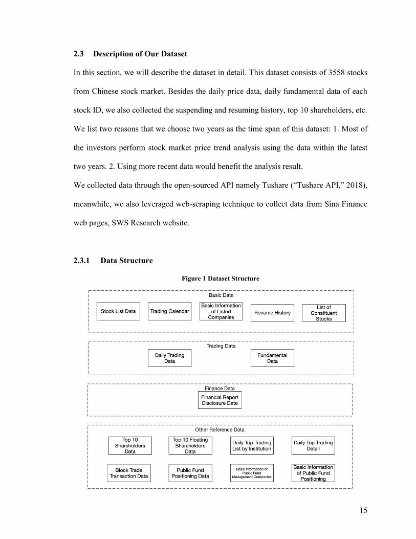
2.3 Description of Our Dataset
In this section, we will describe the dataset in detail. This dataset consists of 3558 stocks
from Chinese stock market. Besides the daily price data, daily fundamental data of each
stock ID, we also collected the suspending and resuming history, top 10 shareholders, etc.
We list two reasons that we choose two years as the time span of this dataset: 1. Most of
the investors perform stock market price trend analysis using the data within the latest
two years. 2. Using more recent data would benefit the analysis result.
We collected data through the open-sourced API namely Tushare (“Tushare API,” 2018),
meanwhile, we also leveraged web-scraping technique to collect data from Sina Finance
web pages, SWS Research website.
2.3.1 Data Structure
Figure 1 Dataset Structure

16
Figure 1 illustrates all the data tables in the dataset.
We collected four categories of data in this dataset: basic data, trading data, finance data,
and other reference data.
All the data tables can be linked by a field called “Stock ID.” It is a unique stock
identifier registered in Chinese Stock market.
Basic Data is the basic information that the researchers might need when exploring the
data. It consists of Stock List Data, Trading Calendar, Basic Information of Listed
Companies, Rename History and List of Constituent Stocks.
Stock List Data: this data table lists the basic information of all the stocks. It has both
Chinese name and English name, as well as other important information such as industry,
market type, list/delist date and stock exchange, etc. While the most useful column is
stock ID, researchers can store the list and look up information in other data tables.
Trading Calendar: trading calendar data table is also for lookup usage. To look up if a
day is a trading date or not. Users can filter the calendar by different stock exchange ID
(SSE or SZSE).
Basic Information of Listed Companies: information about listed companies such as
geography information and line of business. This data table is also arranged by stock ID.
Rename History: history of renaming the stocks, including the start date and end date of
the name also the reason for changing. While the stock ID never changes with the stock
name.
List of Constituent Stocks: if a stock is constituent stock can be counted as a feature.
Users can also get the information about if the constituent stock is newly included.

17
The category called trading data consists of two data types; one is daily trading data;
another one is the fundamental data. They are the core data of this dataset; it consists of
2-year stock trading data from Jan 2017 to Dec 2018.
Daily Trading Data: daily trading data is arranged by stock ID, one stock ID per CSV file.
It consists of 2-year trading data in daily basis from Jan 2017 to Dec 2018, and if the
stock were listed after Jan 2017, the date range would be from the listed date to Dec 2018.
If the stock were delisted before Dec 2018, the data range would be from Jan 2017 to
delist date. If the stock was listed after Jan 2017 and delisted before Dec 2018, the data
range will be from listed date to delisted date. Trading data includes the basic price data
to calculate the technical indices.
Fundamental Data: daily fundamental data is also arranged by stock ID, one stock ID per
CSV file. It consists of 2 years of fundamental data on a daily basis from Jan 2017 to Dec
2018; if the stock were listed after Jan 2017, the date range would be from the listed date
to Dec 2018. If the stock were delisted before Dec 2018, the data range would be from
Jan 2017 to delist date. If the stock was listed after Jan 2017 and delisted before Dec
2018, the data range will be from listed date to delisted date. Different from trading data,
the fundamental data are often used to perform analysis straightforward rather than
calculation.
The third category is the finance data. There wasn’t much finance data available on-line;
we can only get the financial report disclosure date to support the related analysis.
Financial Report Disclosure Date: all the financial report disclosure date data are
arranged within one data table. While researchers can still look up the related information
18
by stock ID, this data table does not include the detailed data of financial reports but only
the scheduled disclosure date and actual disclosure date.
Besides, this dataset also consists of abundant reference data that highly expand the
research opportunities. There are eight data tables of other reference data available. This
data might be used to support related analysis or for feature extension usage.
Top 10 Shareholders Data: data of all the stocks are stored in one data table. Users can
group by stock ID, announcement date, or end date. It is also possible to query by
Shareholder name when the same shareholder holds multiple stocks in the top 10 chart.
Holding amount and holding ratio is available for analysis.
Top 10 Floating Shareholders Data: different from top 10 shareholder chart, this data
table does not include holding ratio since it is for floating shareholders while users can
still group the data by stock ID, announcement and end date, shareholder name.
Daily Top Trading List by Institution: since one institution might operate multiple times
in a day, this data table of the trading transaction is grouped by institutions. Top 10
buyers and top 10 sellers are listed in one same data table may need a further arrangement
for analysis one direction trading.
Daily Top Trading Detail: the top trading transactions detail of all stocks are stored in
one same data table. This data table is transaction-based; the information embedded in
this table is more detailed than the daily top trading list by institutions. Besides the
amount and ratio data, the nominated reason is also included in the data table.
Block Trade Transaction Data: not only top trading transactions are important to stock
price trend analysis, but block trade transaction data is also essential.

19
Public Fund Positioning Data: public fund positioning status is often considered as an
important feature of stock price analysis; it has been proved correlating to the stability of
stock performance. This data table includes the market value and volume, instead of
grouping by stock ID, this data table is grouped by fund ID while researchers can still
rearrange the data into stock ID-based structure as the extended features for further
analysis.
Basic Information of Public Fund Management Companies: most of the information in
this data table are descriptive data about fund management companies.
Basic Information of Public Fund Positioning: most of the information in this data table
are features of the fund. Users can exploit fund ID to other data tables for further analysis.
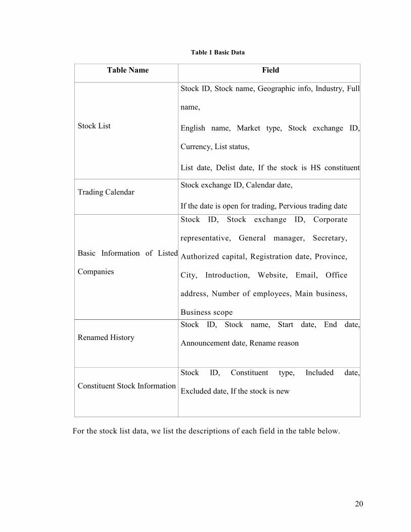
2.3.2 Basic Data
First, we collected the basic data of the Chinese stock market. The function of basic data
is to facilitate data analysis tasks, when researchers using this dataset, they won’t have to
extract basic information mapping table or trading calendar anymore.
The basic data consists of stock list, trading calendar, basic information of listed
companies, renamed history, constituent stock information.
20
Table 1 Basic Data
Table Name Field
Stock List
Stock ID, Stock name, Geographic info, Industry, Full
name,
English name, Market type, Stock exchange ID,
Currency, List status,
List date, Delist date, If the stock is HS constituent
stock Trading Calendar
Stock exchange ID, Calendar date,
If the date is open for trading, Pervious trading date
Basic Information of Listed
Companies
Stock ID, Stock exchange ID, Corporate
representative, General manager, Secretary,
Authorized capital, Registration date, Province,
City, Introduction, Website, Email, Office
address, Number of employees, Main business,
Business scope
Renamed History
Stock ID, Stock name, Start date, End date,
Announcement date, Rename reason
Constituent Stock Information
Stock ID, Constituent type, Included date,
Excluded date, If the stock is new
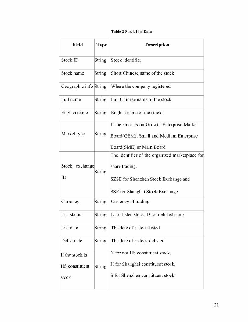
For the stock list data, we list the descriptions of each field in the table below.
21
Table 2 Stock List Data
Field Type Description
Stock ID String Stock identifier
Stock name String Short Chinese name of the stock
Geographic info String Where the company registered
Full name String Full Chinese name of the stock
English name String English name of the stock
Market type String
If the stock is on Growth Enterprise Market
Board(GEM), Small and Medium Enterprise
Board(SME) or Main Board
Stock exchange
ID
String
The identifier of the organized marketplace for
share trading.
SZSE for Shenzhen Stock Exchange and
SSE for Shanghai Stock Exchange
Currency String Currency of trading
List status String L for listed stock, D for delisted stock
List date String The date of a stock listed
Delist date String The date of a stock delisted
If the stock is
HS constituent
stock
String
N for not HS constituent stock,
H for Shanghai constituent stock,
S for Shenzhen constituent stock
22
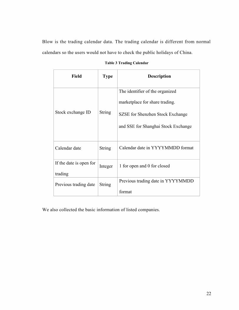
Blow is the trading calendar data. The trading calendar is different from normal
calendars so the users would not have to check the public holidays of China.
Table 3 Trading Calendar
Field Type Description
Stock exchange ID String
The identifier of the organized
marketplace for share trading.
SZSE for Shenzhen Stock Exchange
and SSE for Shanghai Stock Exchange
Calendar date String Calendar date in YYYYMMDD format
If the date is open for
trading
Integer 1 for open and 0 for closed
Previous trading date String Previous trading date in YYYYMMDD
format
We also collected the basic information of listed companies.
23
Table 4 Basic Information of Listed Companies
Field Type Description
Stock ID String Stock identifier
Stock exchange ID String
The identifier of the organized marketplace for
share trading.
SZSE for Shenzhen Stock Exchange
and SSE for Shanghai Stock Exchange Corporate
representative
String The corporate representative of the company
General manager String The general manager of the company
Secretary String The secretary of the chairman of the board
Authorized capital Float The authorized capital of the company
Registration date String When did the company register
Province String Which province does the company locate
City String Which city does the company locate
Introduction String The introduction of the company
Website String The website of the company
Email String The email of the company
Office address String The office address of the company
Number of
employees
Integer Number of employees working in the
company
Main business String Main business of the company
Line of business String Line of business scope
24
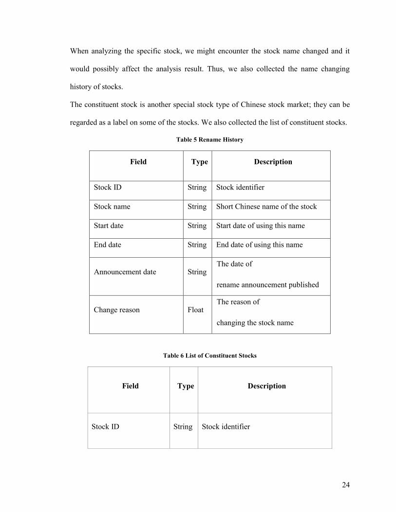
When analyzing the specific stock, we might encounter the stock name changed and it
would possibly affect the analysis result. Thus, we also collected the name changing
history of stocks.
The constituent stock is another special stock type of Chinese stock market; they can be
regarded as a label on some of the stocks. We also collected the list of constituent stocks.
Table 5 Rename History
Field Type Description
Stock ID String Stock identifier
Stock name String Short Chinese name of the stock
Start date String Start date of using this name
End date String End date of using this name
Announcement date String The date of
rename announcement published
Change reason Float The reason of
changing the stock name
Table 6 List of Constituent Stocks
Field Type Description
Stock ID String Stock identifier
25
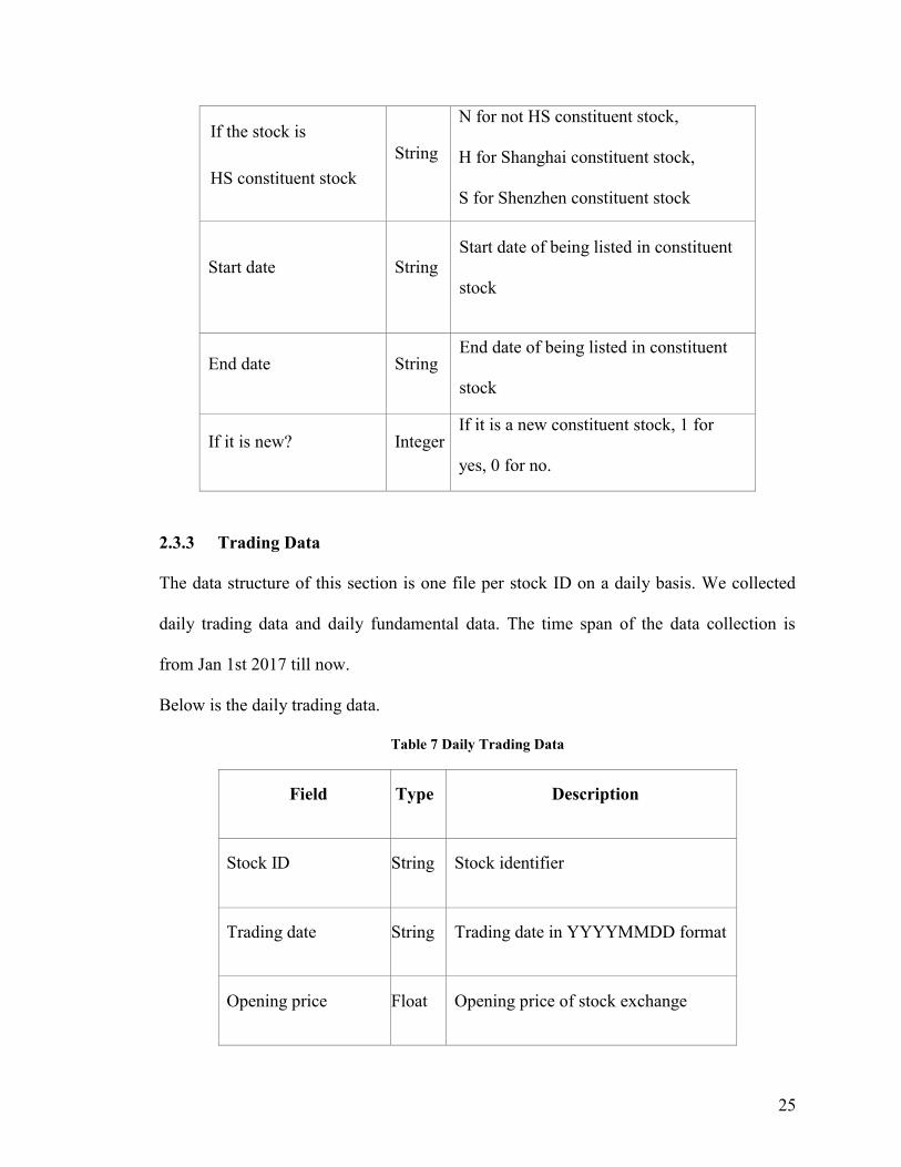
If the stock is
HS constituent stock
String
N for not HS constituent stock,
H for Shanghai constituent stock,
S for Shenzhen constituent stock
Start date String
Start date of being listed in constituent
stock
End date String End date of being listed in constituent
stock
If it is new? Integer If it is a new constituent stock, 1 for
yes, 0 for no.
2.3.3 Trading Data
The data structure of this section is one file per stock ID on a daily basis. We collected
daily trading data and daily fundamental data. The time span of the data collection is
from Jan 1st 2017 till now.
Below is the daily trading data.
Table 7 Daily Trading Data
Field Type Description
Stock ID String Stock identifier
Trading date String Trading date in YYYYMMDD format
Opening price Float Opening price of stock exchange
26
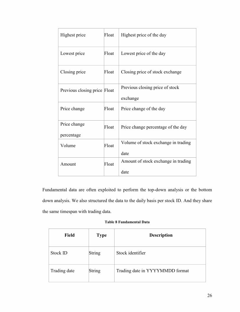
Highest price Float Highest price of the day
Lowest price Float Lowest price of the day
Closing price Float Closing price of stock exchange
Previous closing price Float Previous closing price of stock
exchange
Price change Float Price change of the day
Price change
percentage
Float Price change percentage of the day
Volume Float Volume of stock exchange in trading
date
Amount Float Amount of stock exchange in trading
date
Fundamental data are often exploited to perform the top-down analysis or the bottom
down analysis. We also structured the data to the daily basis per stock ID. And they share
the same timespan with trading data.
Table 8 Fundamental Data
Field Type Description
Stock ID String Stock identifier
Trading date String Trading date in YYYYMMDD format
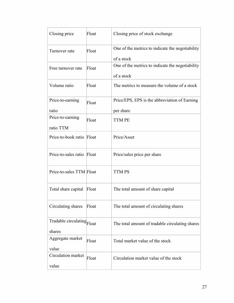
27
Closing price Float Closing price of stock exchange
Turnover rate Float One of the metrics to indicate the negotiability
of a stock
Free turnover rate Float One of the metrics to indicate the negotiability
of a stock
Volume ratio Float The metrics to measure the volume of a stock
Price-to-earning
ratio
Float Price/EPS, EPS is the abbreviation of Earning
per share
Price-to-earning
ratio TTM
Float TTM PE
Price-to-book ratio Float Price/Asset
Price-to-sales ratio Float Price/sales price per share
Price-to-sales TTM Float TTM PS
Total share capital Float The total amount of share capital
Circulating shares Float The total amount of circulating shares
Tradable circulating
shares
Float The total amount of tradable circulating shares
Aggregate market
value
Float Total market value of the stock
Circulation market
value
Float Circulation market value of the stock
28
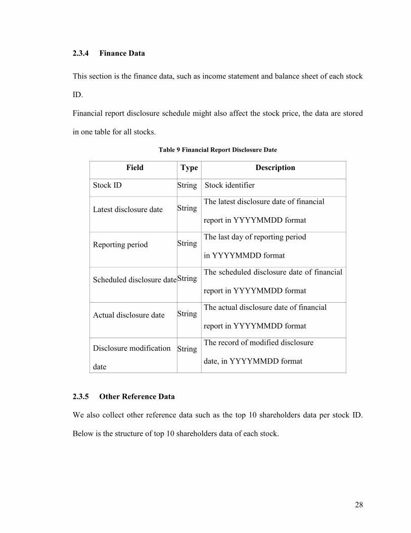
2.3.4 Finance Data
This section is the finance data, such as income statement and balance sheet of each stock
ID.
Financial report disclosure schedule might also affect the stock price, the data are stored
in one table for all stocks.
Table 9 Financial Report Disclosure Date
Field Type Description
Stock ID String Stock identifier
Latest disclosure date String The latest disclosure date of financial
report in YYYYMMDD format
Reporting period String The last day of reporting period
in YYYYMMDD format
Scheduled disclosure date String The scheduled disclosure date of financial
report in YYYYMMDD format
Actual disclosure date String The actual disclosure date of financial
report in YYYYMMDD format
Disclosure modification
date
String The record of modified disclosure
date, in YYYYMMDD format
2.3.5 Other Reference Data
We also collect other reference data such as the top 10 shareholders data per stock ID.
Below is the structure of top 10 shareholders data of each stock.

29
Table 10 Top 10 Shareholders Data
Field Type Description
Stock ID String Stock identifier
Announcement
date
String
Announcement date in YYYYMMDD
format
End date String Reporting date in YYYYMMDD format
Shareholder name String Name of the shareholder
Holding amount Float Stock holding amount (per unit of stock)
Holding ratio Float Stock holding ratio
Besides, we also collect the top 10 floating shareholders data for the stocks in basic
information scope for comparison purpose.
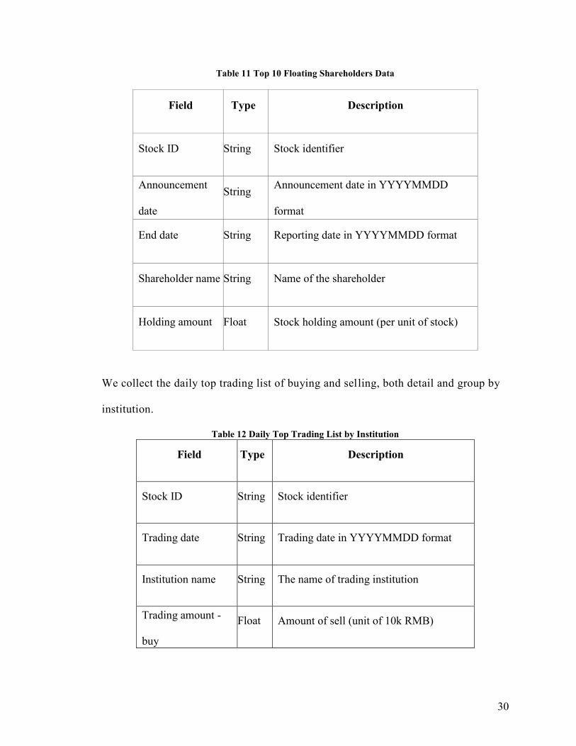
30
Table 11 Top 10 Floating Shareholders Data
Field Type Description
Stock ID String Stock identifier
Announcement
date
String Announcement date in YYYYMMDD
format
End date String Reporting date in YYYYMMDD format
Shareholder name String Name of the shareholder
Holding amount Float Stock holding amount (per unit of stock)
We collect the daily top trading list of buying and selling, both detail and group by
institution.
Table 12 Daily Top Trading List by Institution
Field Type Description
Stock ID String Stock identifier
Trading date String Trading date in YYYYMMDD format
Institution name String The name of trading institution
Trading amount -
buy
Float Amount of sell (unit of 10k RMB)
31
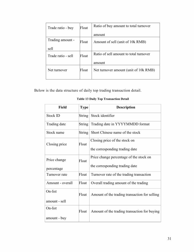
Trade ratio - buy Float Ratio of buy amount to total turnover
amount
Trading amount -
sell
Float Amount of sell (unit of 10k RMB)
Trade ratio - sell Float Ratio of sell amount to total turnover
amount
Net turnover Float Net turnover amount (unit of 10k RMB)
Below is the data structure of daily top trading transaction detail.
Table 13 Daily Top Transaction Detail
Field Type Description
Stock ID String Stock identifier
Trading date String Trading date in YYYYMMDD format
Stock name String Short Chinese name of the stock
Closing price Float Closing price of the stock on
the corresponding trading date
Price change
percentage
Float Price change percentage of the stock on
the corresponding trading date
Turnover rate Float Turnover rate of the trading transaction
Amount - overall Float Overall trading amount of the trading
transaction On-list
amount - sell
Float Amount of the trading transaction for selling
On-list
amount - buy
Float Amount of the trading transaction for buying
32
On-list
turnover
Float Turnover of the trading transaction
On-list
net trading amount
Float Net trading amount of the trading transaction
On-list
net trading ratio
Float Ratio of net trading amount to overall trading
amount
On-list
net turnover ratio
Float Ratio of on-list net turnover to overall
turnover
Circulation market
value
Float Circulation market value of the stock
Reason String Reason of being nominated.
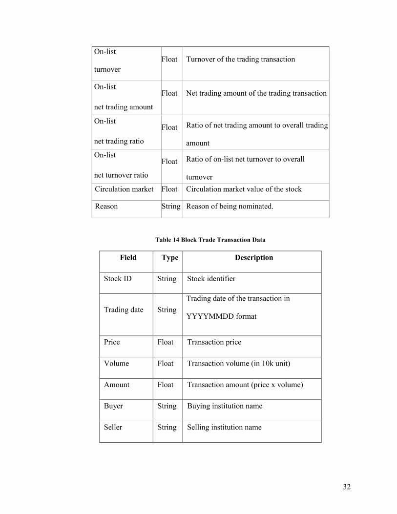
Table 14 Block Trade Transaction Data
Field Type Description
Stock ID String Stock identifier
Trading date String
Trading date of the transaction in
YYYYMMDD format
Price Float Transaction price
Volume Float Transaction volume (in 10k unit)
Amount Float Transaction amount (price x volume)
Buyer String Buying institution name
Seller String Selling institution name

33
Besides the shareholder related data, the block trade data is also considered as one of the
factors that may affect the stock price trend that worth to investigate.
Since many of the investors mentioned how fund positioning affect stock market price
trend, we also collect the fund positioning data as an important part of reference data.
Please be aware that the fund data are public fund data only, which can also be fund on
public financial web sites.
The basic information of fund management company is for further data mining purpose.
The data structure is illustrated as the table below.
Besides, the basic information on fund positioning data is summarized in one data table.
This is a positioning transaction-based data table.
Table 15 Public Fund Positioning Data
Field Type Description
Fund ID String Public fund identifier
Announcement
date
String
Announcement date of positioning in
YYYYMMDD format
End date String
The end date of positioning
in YYYYMMDD format
Stock ID String Stock identifier
Market value Float Positioning market value (Yuan)
Volume Float Positioning volume (per unit of stock)

34
Market value ratio Float
The ratio of occupied market value of
positioning to overall market value
Circulation market
value ratio
Float
The ratio of occupied circulation
market value of positioning to overall
circulation market value
2.4 Research Opportunity
Since we have collected a variety of data, the research opportunity is abundant. First, the
daily trading data is available; the researchers can use the fundamental price information
to calculate most of the technical indices. Moreover, researchers can also model the
technical indices with fundamental prices in two years to time sequence and make the
price or trend prediction.
Not only can the price and technical indices be used as features, but other information
gathered in the dataset can also potentially be used as features and serves for data mining
purpose.
For example, many previous works involve sentiment analysis in their proposed solutions.
With the essential information in our dataset, researchers can perform web-scraping to
get the related public information from websites. Or they could leverage the news
scraping on social media to supervise how social media post affect the stock market price,
which makes a real-time sentiment analysis system on the stock market possible.
35
Chapter 3: Survey of Related works
In this section, we will introduce the previous works. We reviewed related work in two
different domains: technical and financial, respectively. While the financial domain
literature review can be found in chapter 2.2 for providing the direction of data collection,
this part is the literature review of the technical domain.
3.1 Technical Related Works
Kim and Han in (Kim & Han, 2000) built a new hybrid model of artificial neural
networks (ANN) and used genetic algorithms (GAs) approach to feature discretization for
predicting stock price index. The research data used in this study is technical indicators
and the direction of change in the daily Korea stock price index (KOSPI). The total
number of samples is 2928 trading days, from January 1989 to December 1998. Table 16
gives selected features and their formulas (Achelis, 1995; Chang, Jung, Yeon, Jun, Shin
& Kim, 1996; Choi, 1995; Edwards & Magee, 1997; Gifford, 1995). They also applied
optimization of feature discretization, closely related to the dimensionality reduction.
The strengths of their work are that they introduced GA to optimize the ANN, also listed
the selected features in Table 16. However, we also found some weaknesses existed in
this paper. First, the amount of input features and processing elements in the hidden layer
is 12 and not adjustable. Another limitation is in the learning process of ANN; the
authors only focused on two factors in optimization. While they still believed that GA has
great potential for feature discretization optimization. Our initialized feature pool refers
to the selected features in Table 16. The algorithm they used to improve the ANN
performance was GA, which is popularly used to optimize relevant feature subset or

36
determine the number of processing elements and hidden layers. So, we include ANN for
model performance comparison.
Piramuthu in (Piramuthu, 2004) conducted a thorough evaluation of different feature
selection methods for data mining applications. He used for datasets which were credit
approval data, loan defaults data, web traffic data, tam and kiang data, and compared how
different feature selection methods optimized decision tree performance. The feature
selection methods he compared included probabilistic distance measure: the
Bhattacharyya measure, the Matusita measure, the divergence measure, the Mahalanobis
distance measure, and the Patrick-Fisher measure. For inter-class distance measures: the
Minkowski distance measure, city block distance measure, Euclidean distance measure,
the Chebychev distance measure, and the nonlinear (Parzen and hyper-spherical kernel)
distance measure. The strength of this paper is that the author evaluated both probabilistic
distance-based and several inter-class feature selection methods. Besides, the author
performed the evaluation based on different datasets, which reinforced the strength of this
paper. However, the evaluation algorithm was a decision tree only. We cannot conclude
if the feature selection methods will still perform the same on a larger dataset or a more
complex model. This paper introduced a method for feature selection. Since there are a
large number of features in the stock market, irrelevant features will affect the
performance, so we would like to investigate the feature selection approaches. The author
also found that the nonlinear measure often performed well in most cases.
Hassan and Nath in (Hassan & Nath, 2005) applied Hidden Markov Model (HMM) on
the stock market forecasting on stock prices of four different Airlines. They reduce states
of the model into four states: opening price, closing price, the highest price, and the

37
lowest price. The strong point of this paper is that the approach does not need expert
knowledge to build a prediction model. While this work is limited within the industry of
Airlines, and evaluated on a very small dataset, may not lead to a prediction model with
generality. One of the approaches in stock market prediction related works could be
exploited to do the comparison work. The authors selected maximum 2 years as the date
range of training and testing dataset, which provided us a date range reference for our
evaluation part.
Lei in (Lei, 2018) exploited Wavelet Neural Network (WNN) to predict stock price trend.
The author also applied Rough Set (RS) for attribute reduction as an optimization. Rough
Set was exploited to reduce the stock price trend feature dimensions. It was also used to
determine the structure of Wavelet Neural Network. The dataset of this work consists of
5 famous stock market indices. SSE Composite Index (China), CSI 300 Index (China),
All Ordinaries Index (Australian), Nikkei 225 Index (Japan) and Dow Jones Index (USA).
The model evaluation was based on different stock market indices, the result was
convincing with generality. By using Rough Set for optimizing the feature dimension
before processing reduces the computational complexity. However, the author only
stressed the parameter adjustment in discussion part but didn’t specify the weakness of
the model itself. Meanwhile, we also found that the evaluations were performed on
indices, the same model may not have the same performance if applied on a specific
stock. The features table and calculation formula are worth taking as a reference. They
can also include RS as a method for attribute discretization before processing the data.
Lee in (M. C. Lee, 2009) used the support vector machine (SVM) with a hybrid feature
selection method to perform the stock trend prediction. The dataset in this research
38
project is a sub data set of NASDAQ Index from Taiwan Economic Journal database
(TEJD, 2008). The feature selection part was using a hybrid method, supported sequential
forward search (SSFS) played the role of the wrapper. Another advantage of this work is
that they designed a detailed procedure of parameter adjustment with performance under
different parameter values. The clear structure of feature selection model is also heuristic
to the primary stage of model structuring. One of the limitations was that the author
completed the performance evaluation of SVM to compare with back-propagation neural
network (BPNN) only, while did not compare with other machine learning algorithms.
Table 2 listed the results of F-score and average accuracy rate of selected features. The
author also found that the combination of the SVM-based model and F _SSFS served as a
promising method in stock trend prediction.
Sirignano and Cont leveraged a deep learning approach trained on a universal feature set
of financial markets in (Sirignano & Cont, 2018). The data set they used was a high-
frequency electronic buy and sell records of all transactions, and cancellations of orders
for approximately 1000 NASDAQ stocks through the exchange’s order book. The NN
consists of 3 layers with LSTM units followed by a feed-forward layer with rectified
linear units (ReLUs) at last, with stochastic gradient descent (SGD) algorithm as an
optimization. A fruitful paper on modeling mega data. Their universal model was able to
generalize to stocks outside of the training sample. Though they mentioned the
advantages of a universal model, the training cost was still expensive. Meanwhile, due to
the inexplicit programming of the deep learning algorithm, we don’t know if there are
useless features adulterated when feeding the data into the model. It would be better if
they perform a feature selection part before training the model, and it is also an effective

39
way to reduce the computational complexity. First, the paper proved that the price
information in the financial market has universal features. The features they extracted
were trained from all stocks, which also proved the value of our work in stock price trend
analysis. They also proved that to build a large model without overfitting on financial
data is possible.
Ni et al. in (Ni, Ni, & Gao, 2011) predicted stock price trend by exploiting SVM and
performed fractal feature selection for optimization. The dataset they used is Shanghai
Stock Exchange Composite Index (SSECI) with 19 technical indicators as features.
Before processing the data, they optimized the input data by performing feature selection.
When finding the best parameter combination, they also used a grid search method which
is k-cross-validation. Besides, the evaluation of different feature selection methods is also
comprehensive. As the authors mentioned in their conclusion part, they only considered
the technical indicators but not macro and micro factors in financial domain. The source
of datasets that authors used were similar to our dataset, which makes their evaluation
results useful to our research. They also mentioned a method called k-cross-validation
when testing hyper-parameter combinations.
McNally et al. in (McNally, Roche, & Caton, 2018) leveraged RNN and LSTM on
predicting the price of Bitcoin, optimized by using Boruta algorithm for feature
engineering part, it works similarly to the random forest classifier. Besides feature
selection, they also used Bayesian optimization to select LSTM parameters. The Bitcoin
dataset ranged from the 19th of August 2013 to 19th of July 2016. Used multiple
optimization methods to improve the performance of deep learning methods. The primary
problem of their work is overfitting. The research problem of predicting Bitcoin price

40
trend has some similarities with stock market price prediction. Hidden features and noises
embedded in the price data are threats of this work, the authors treated the research
question as a time sequence problem. The best part of this paper is feature engineering
and optimization part; we could replicate the methods they exploited in our data pre-
processing.
Weng et al. in (Weng, Lu, Wang, Megahed, & Martinez, 2018) focused on short-term
stock prices prediction by using ensemble methods of four commonly used machine
learning models. The dataset for this project is five sets of data, they obtained these
datasets from three open-sourced APIs and the TTR R package. The four commonly used
machine learning models are a neural network regression ensemble (NNRE), a Random
Forest with unpruned regression trees as base learners (RFR), AdaBoost with unpruned
regression trees as base learners (BRT) and a support vector regression ensemble (SVRE).
A thorough study of ensemble methods specified for short-term stock price prediction.
With background knowledge, authors selected eight technical indicators in this study then
performed a thoughtful evaluation of five datasets. The primary contribution of this paper
is that they developed a platform for investors using R, which does not need users to
input their own data but call API to fetch the data from online source straightforward.
From the research perspective, they only evaluated the prediction of the price for 1 up to
10 days ahead but did not evaluate longer terms than two trading weeks or a shorter term
than 1 day. The primary limitation of their research was that they only analyzed 20 U.S.-
based stocks, the model might not be generalized to other stock market or need further
revalidation to see if it suffered from overfitting problems. The core content that related
41
to our work is the feature extraction and evaluation. They illustrated how they performed
feature extraction in detail and also listed the formula for evaluation.
Kara et al. in (Kara, Acar Boyacioglu, & Baykan, 2011) also exploited ANN and SVM in
predicting the stock price index movement. The entire data set covers the period from
January 2, 1997, to December 31, 2007, of Istanbul Stock Exchange. The primary
strength of this work is their detailed record of parameter adjustment procedures. While
the weaknesses of this work are: neither the technical indicator nor the model structure
has novelty, and the authors didn’t explain how their model performed better than other
models in previous works, thus more validation works on other datasets would help. They
explained how ANN and SVM work with stock market features, also recorded the
parameter adjustment. The implementation part of our research could benefit from this
previous work.
Jeon et al. in (Jeon, Hong, & Chang, 2018) performed research on millisecond interval-
based big dataset by using pattern graph tracking to complete stock price prediction task.
The dataset they used is a millisecond interval-based big dataset of historical stock data
from KOSCOM, from August 2014 to October 2014, 10G-15G capacity. The author
applied Euclidean distance, Dynamic Time Warping (DTW) for pattern recognition. For
feature selection, they used stepwise regression. The authors completed the prediction
task by ANN, and Hadoop and RHive for big data processing. Evaluation section is based
on the result processed by a combination of SAX and Jaro-Winkler distance. Before
processing the data, they generated aggregated data at five-minute intervals from discrete
data. The primary strength of this work is the explicit structure of the whole
implementation procedure. While they exploited a relatively old model, another weakness
42
is the overall time span of the training data is extremely short. It is difficult to access the
millisecond interval-based data in real life, so the model is not as practical as a daily
based data model. The evaluation is only based on three specific stocks in the Republic of
Korea. But this work is highly recommended because rather than performing prediction
on a small amount of data, this is one of the latest papers in stock price prediction using
big data. The SAX and Jaro-Winkler distance methods are worth taking as a reference in
our evaluation part.
Huang et al. in (C. F. Huang, Chang, Cheng, & Chang, 2012) applied a fuzzy-GA model
to complete the stock selection task. They used the constituent stocks of the 200 largest
market capitalization listed in the Taiwan Stock Exchange as the investment universe.
Besides, the yearly financial statement data and stock returns were retrieved from the TEJ
(Taiwan Economic Journal Co. Ltd., http://www.tej.com.tw/) database for the period of
time from 1995 to 2009. For optimization, they conducted the fuzzy membership function
with GA-optimized model parameters and extracted features for stock scoring purpose.
The authors proposed an optimized model for stock selection and scoring. Different from
the prediction model, the authors more focused on stock rankings, selection and
performance evaluation, their structure is more practical among investors. But in the
model validation part, they did not compare the model with existed algorithms but the
statistics of the benchmark, which made it challenging to identify if GA would
outperform other algorithms. The most valuable part of their work was the attributes they
used in their stock selection model. The authors listed both formula and the references of
each attribute. Besides the attributes, they also listed the statistics of benchmarks, it
provides us a structure of evaluating machine learning models.
43
Fischer and Krauss in (Fischer & Krauss, 2018) applied long short-term memory (LSTM)
on financial market prediction. The dataset they used is S&P 500 index constituents from
Thomson Reuters. They obtained all month-end constituent lists for the S&P 500 from
Dec 1989 to Sep 2015, then consolidate the lists into a binary matrix to eliminate survivor
bias. The authors also used RMSprop as an optimizer, which is a mini-batch version of
rprop. The primary strength of this work is that the authors used the latest deep learning
technique to perform financial market predictions. On the other hand, they relied on
LSTM technique, lack of background knowledge in financial domain. Though the LSTM
outperformed the standard DNN and logistic regression algorithms, while the author did
not mention the effort to train an LSTM with long-time dependencies. Their works
indicated that LSTM is suitable for financial time series prediction tasks. With a thorough
evaluation work, they drew a conclusion that LSTM outperforms the standard DNN and
logistic regression marginally. It provided us a direction of choosing an algorithm to
model the data if the goal is investigating the time series problem in the stock market.
Tsai and Hsiao in (Tsai & Hsiao, 2010) combined multiple feature selection methods for
stock prediction. The data source is Taiwan Economic Journal (TEJ) database. The time
range of the data is from the first quarter of 2000 to the second quarter of 2007. They
exploited sliding window method combined with multi-layer perceptron (MLP) artificial
neural networks with the back-propagation learning algorithm as a baseline prediction
model. Besides they also applied principal component analysis (PCA) for dimension
reduction, Genetic Algorithms (GA) and the classification and regression trees (CART)
for feature selection. Unlike other previous works that took technical indices in
consideration only, the data set they analyzed included both fundamental and
44
macroeconomic indices. The authors also compared the feature selection method
combinations. Also, the validation part was done by combining the model performance
stats with statistical analysis. The principal component analysis they performed was the
basic method. There is another variance of PCA approaches such as asymmetric PCA and
kernel PCA. We took a similar structure to the literature review part of this work.
Another part worth taking as reference was the fundamental and macroeconomic indices.
Pimenta et al. in (Pimenta, Nametala, Guimarães, & Carrano, 2018) leveraged an
automated investing method by using multi-objective genetic programming and applied it
in the stock market. The dataset was obtained from Brazilian stock exchange market
(BOVESPA), and the primary techniques they exploited were a combination of multi-
objective optimization, genetic programming, and technical trading rules. For
optimization, they leveraged genetic programming (GP) to optimize decision rules. The
novelty of this paper was in the evaluation part. They included a historical period, which
was a critical moment of Brazilian politics and economics when performing validation.
This approach reinforced the generalization strength of their proposed model. When
selecting the sub-dataset for evaluation, they also set criteria to ensure more assets
liquidity. While the baseline of the comparison was too basic and fundamental, and the
authors didn’t perform any comparison with other existing models. The author listed the
parameters of their automated system. We consider using the same overall structure to
design a prediction model to fit the model on other financial market data, which is a
practical approach to increase the model generality.
Huang and Tsai in (C. L. Huang & Tsai, 2009) conducted a filter-based feature selection
assembled with a hybrid self-organizing feature map (SOFM) support vector regression

45
(SVR) model to forecast Taiwan index futures (FITX) trend. They divided the training
samples into clusters to marginally to improve the training efficiency. The authors
proposed a comprehensive model which was a combination of two novel machine
learning techniques in stock market analysis. Besides, the optimizer of feature selection
was also applied before the data processing to improve the prediction accuracy and
reduce the computational complexity of processing daily stock index data. Though they
optimized the feature selection part and split the sample data into small clusters, it was
already strenuous to train daily stock index data of this model. It would be difficult for
this model to predict trading activities in shorter time intervals since the data volume
would be increased drastically. Moreover, the evaluation part is not strong enough since
they set a single SVR model as a baseline, but didn’t compare the performance with other
previous works, which caused difficulty for future researchers to identify the advantages
of SOFM-SVR model why it outperforms other algorithms. Overall, their work is a good
comparison with other previous works since it has a common structure. We would take
their technical attributes and compare with attributes from other works, to identify the
similarities and gaps between each work.
Thakur and Kumar in (Thakur & Kumar, 2018) also developed a hybrid financial trading
support system by exploiting multi-category classifiers and random forest (RAF). They
conducted their research on stock indices from NASDAQ, DOW JONES, S&P 500,
NIFTY 50 and NIFTY BANK. The authors proposed a hybrid model combined random
forest (RF) algorithms with weighted multicategory generalized eigenvalue support
vector machine (WMGEPSVM) to generate “Buy/Hold/Sell” signals. Before processing
the data, they used Random Forest (RF) for feature pruning. The authors proposed a

46
practical model designed for real-life investment activities which could generate three
basic signals for investors to refer to. They also performed a thorough comparison
between related algorithms, reinforced the strengths of their evaluation part. While they
didn’t mention the time and computational complexity of their works. Meanwhile, the
unignorably issue of their work was the lack of financial domain knowledge background.
The investors regard the indices data as one of the attributes, but could not take the signal
from indices to operate a specific stock straightforward. Though the system of advising
trading activity and calculating profit is relatively naive, while the signals that generated
from their system still worth referring to. Besides, they also listed the technical attributes
so we could compare the attributes with other works and find the most commonly used
attributes in the stock market price or trend prediction domain.
Hsu in (Hsu, 2013) assembled feature selection with a back propagation neural network
(BNN) combined with genetic programming to predict the stock/futures price. The
dataset in this research project was obtained from Taiwan Stock Exchange Corporation
(TWSE). The authors have introduced the description of the background knowledge in
detail. While the weakness of their work is that it is a lack of data set description. This is
a combination of model that proposed by other previous works. Though we didn’t see the
novelty of this work, we can still conclude that genetic programming (GP) algorithm is
admitted in stock market research domain. To reinforce the validation strengths, it would
be good to consider adding GP models into evaluation if the model is predicting a
specific price.
Hafezi et al. in (Hafezi, Shahrabi, & Hadavandi, 2015) built a bat-neural network multi-
agent system (BN-NMAS) to predict stock price. The dataset was obtained from the

47
deutsche bundes-bank. They also applied bat algorithm (BA) for optimizing neural
network weights. The authors illustrated their overall structure and logic of system design
in clear flowcharts. While there was very few previous works that had performed on
DAX data, it would be difficult to recognize if the model they proposed still has the
generality if migrated on other datasets. The system design and feature selection logic are
fascinating which worth referring to. Their findings in optimization algorithms are also
valuable for the research in stock market prices prediction research domain, it is worth
trying bat algorithm (BA) when constructing neural network models.
Long et al. in (Long, Lu, & Cui, 2018) conducted deep learning approach to predict the
stock price movement. The dataset they used is Chinese stock market index CSI 300. For
predicting the stock price movement, they constructed a multi-filter neural network
(MFNN) with stochastic gradient descent (SGD) and back propagation optimizer for
learning NN parameters. The strength of this paper is that the authors exploited a novel
model with a hybrid model constructed by different kinds of neural networks, it provides
an inspiration of constructing hybrid neural network structures. However, they used a
regular optimizer and did not consider the time and computational complexity of their
proposed model. Their work was a combination of different NNs, which was a valuable
reference of feature mapping and how to deal with overfitting problems.
Atsalakis and Valavanis in (Atsalakis & Valavanis, 2009) proposed a solution of a neuro-
fuzzy system, which is composed of an Adaptive Neuro Fuzzy Inference System (ANFIS)
controller to achieve short-term stock price trend prediction. The noticeable strength of
this work is the evaluation part. Not only did they compare their proposed system with
the popular data models, but also compared with investment strategies. While the

48
weakness that we found from their proposed solution is that their solution architecture is
lack of optimization part, which might limit their model performance. Since our proposed
solution is also focusing on short-term stock price trend prediction, this work is heuristic
for our system design. Meanwhile, by comparing with the popular trading strategies from
investors, their work inspired us to compare the strategies used by investors with
techniques used by researchers.
Nekoeiqachkanloo et al. in (Nekoeiqachkanloo, Ghojogh, Pasand, & Crowley, 2019)
proposed a system with two different approaches for stock investment. The strengths of
their proposed solution are obvious. First, it is a comprehensive system that consists of
data pre-processing and two different algorithms to suggest the best investment portions.
Second, the system also embedded with a forecasting component which also retains the
features of time series. Last but not least, their input features are a mix of fundamental
features and technical indices which aims to fill in the gap between financial domain and
technical domain. However, their work has a weakness in evaluation part. Instead of
evaluating the proposed system on a large dataset, they chose 25 well-known stocks.
There is a high possibility that the well-known stocks might potentially share some
common hidden features. Thus, some other related works randomly sampled stocks from
datasets to perform the evaluation as a denoise method. The data pre-processing part
before feeding the technical indices into time series forecasting component is heuristic to
our system design.
As another related latest work, Idrees et al. (Idrees, Alam, & Agarwal, 2019) published a
time series-based prediction approach for the volatility of the stock market. ARIMA is
not a new approach in time series prediction research domain, their work is more
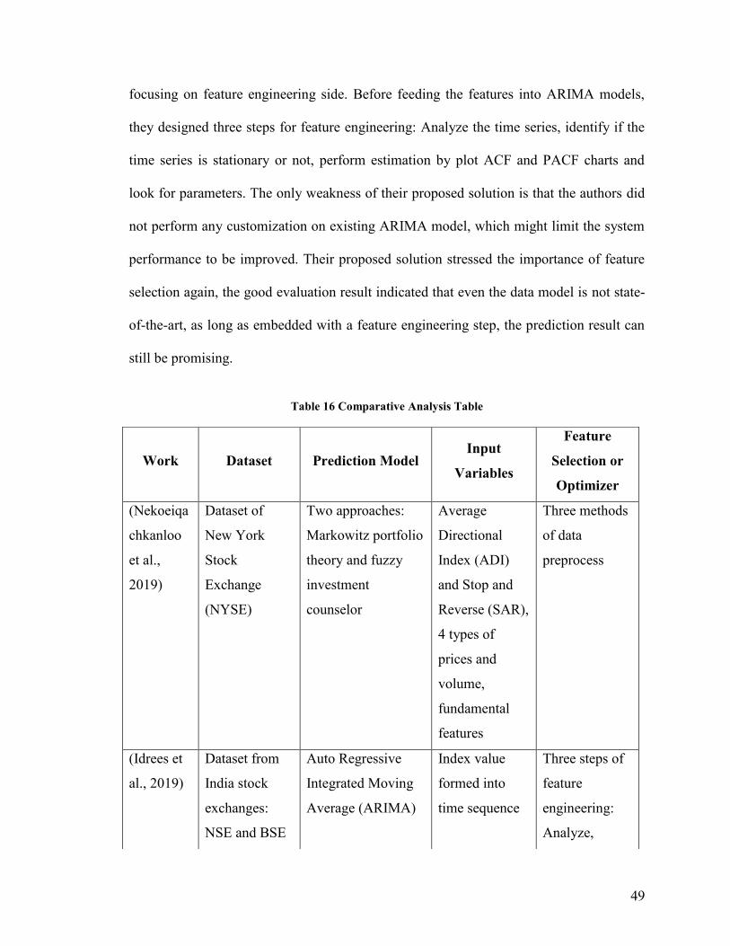
49
focusing on feature engineering side. Before feeding the features into ARIMA models,
they designed three steps for feature engineering: Analyze the time series, identify if the
time series is stationary or not, perform estimation by plot ACF and PACF charts and
look for parameters. The only weakness of their proposed solution is that the authors did
not perform any customization on existing ARIMA model, which might limit the system
performance to be improved. Their proposed solution stressed the importance of feature
selection again, the good evaluation result indicated that even the data model is not state-
of-the-art, as long as embedded with a feature engineering step, the prediction result can
still be promising.
Table 16 Comparative Analysis Table
Work Dataset Prediction Model Input
Variables
Feature
Selection or
Optimizer
(Nekoeiqa
chkanloo
et al.,
2019)
Dataset of
New York
Stock
Exchange
(NYSE)
Two approaches:
Markowitz portfolio
theory and fuzzy
investment
counselor
Average
Directional
Index (ADI)
and Stop and
Reverse (SAR),
4 types of
prices and
volume,
fundamental
features
Three methods
of data
preprocess
(Idrees et
al., 2019)
Dataset from
India stock
exchanges:
NSE and BSE
Auto Regressive
Integrated Moving
Average (ARIMA)
Index value
formed into
time sequence
Three steps of
feature
engineering:
Analyze,
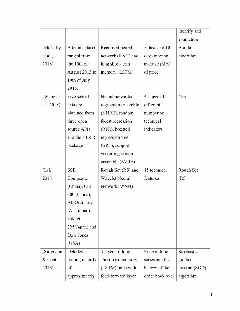
50
identify and
estimation
(McNally
et al.,
2018)
Bitcoin dataset
ranged from
the 19th of
August 2013 to
19th of July
2016.
Recurrent neural
network (RNN) and
long short-term
memory (LSTM)
5 days and 10
days moving
average (MA)
of price
Boruta
algorithm
(Weng et
al., 2018)
Five sets of
data are
obtained from
three open
source APIs
and the TTR R
package
Neural networks
regression ensemble
(NNRE), random
forest regression
(RFR), boosted
regression tree
(BRT), support
vector regression
ensemble (SVRE)
4 stages of
different
number of
technical
indicators
N/A
(Lei,
2018)
SSE
Composite
(China), CSI
300 (China),
All Ordinaries
(Australian),
Nikkei
225(Japan) and
Dow Jones
(USA)
Rough Set (RS) and
Wavelet Neural
Network (WNN).
15 technical
features
Rough Set
(RS)
(Sirignano
& Cont,
2018)
Detailed
trading records
of
approximately
3 layers of long
short-term memory
(LSTM) units with a
feed-forward layer
Price in time-
series and the
history of the
order book over
Stochastic
gradient
descent (SGD)
algorithm
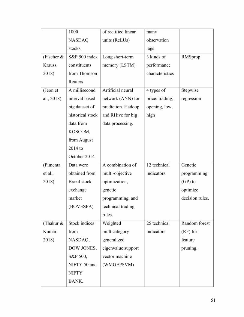
51
1000
NASDAQ
stocks
of rectified linear
units (ReLUs)
many
observation
lags
(Fischer &
Krauss,
2018)
S&P 500 index
constituents
from Thomson
Reuters
Long short-term
memory (LSTM)
3 kinds of
performance
characteristics
RMSprop
(Jeon et
al., 2018)
A millisecond
interval based
big dataset of
historical stock
data from
KOSCOM,
from August
2014 to
October 2014
Artificial neural
network (ANN) for
prediction. Hadoop
and RHive for big
data processing.
4 types of
price: trading,
opening, low,
high
Stepwise
regression
(Pimenta
et al.,
2018)
Data were
obtained from
Brazil stock
exchange
market
(BOVESPA)
A combination of
multi-objective
optimization,
genetic
programming, and
technical trading
rules.
12 technical
indicators
Genetic
programming
(GP) to
optimize
decision rules.
(Thakur &
Kumar,
2018)
Stock indices
from
NASDAQ,
DOW JONES,
S&P 500,
NIFTY 50 and
NIFTY
BANK.
Weighted
multicategory
generalized
eigenvalue support
vector machine
(WMGEPSVM)
25 technical
indicators
Random forest
(RF) for
feature
pruning.
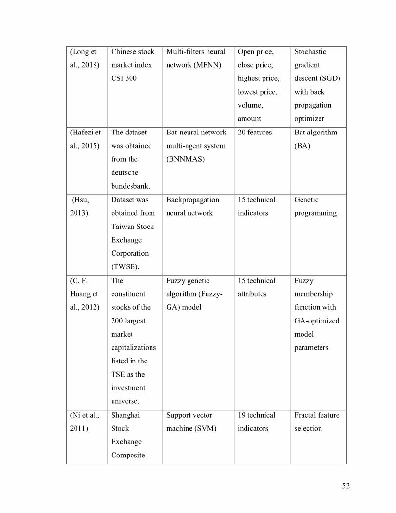
52
(Long et
al., 2018)
Chinese stock
market index
CSI 300
Multi-filters neural
network (MFNN)
Open price,
close price,
highest price,
lowest price,
volume,
amount
Stochastic
gradient
descent (SGD)
with back
propagation
optimizer
(Hafezi et
al., 2015)
The dataset
was obtained
from the
deutsche
bundesbank.
Bat-neural network
multi-agent system
(BNNMAS)
20 features Bat algorithm
(BA)
(Hsu,
2013)
Dataset was
obtained from
Taiwan Stock
Exchange
Corporation
(TWSE).
Backpropagation
neural network
15 technical
indicators
Genetic
programming
(C. F.
Huang et
al., 2012)
The
constituent
stocks of the
200 largest
market
capitalizations
listed in the
TSE as the
investment
universe.
Fuzzy genetic
algorithm (Fuzzy-
GA) model
15 technical
attributes
Fuzzy
membership
function with
GA-optimized
model
parameters
(Ni et al.,
2011)
Shanghai
Stock
Exchange
Composite
Support vector
machine (SVM)
19 technical
indicators
Fractal feature
selection
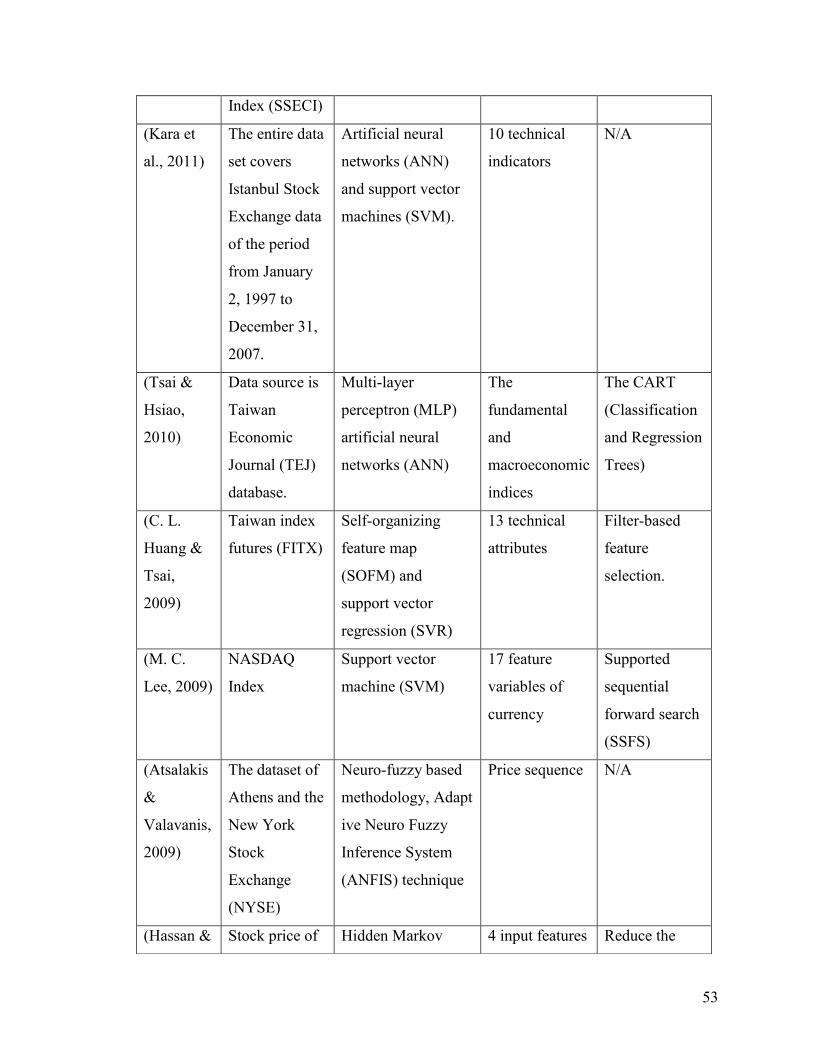
53
Index (SSECI)
(Kara et
al., 2011)
The entire data
set covers
Istanbul Stock
Exchange data
of the period
from January
2, 1997 to
December 31,
2007.
Artificial neural
networks (ANN)
and support vector
machines (SVM).
10 technical
indicators
N/A
(Tsai &
Hsiao,
2010)
Data source is
Taiwan
Economic
Journal (TEJ)
database.
Multi-layer
perceptron (MLP)
artificial neural
networks (ANN)
The
fundamental
and
macroeconomic
indices
The CART
(Classification
and Regression
Trees)
(C. L.
Huang &
Tsai,
2009)
Taiwan index
futures (FITX)
Self-organizing
feature map
(SOFM) and
support vector
regression (SVR)
13 technical
attributes
Filter-based
feature
selection.
(M. C.
Lee, 2009)
NASDAQ
Index
Support vector
machine (SVM)
17 feature
variables of
currency
Supported
sequential
forward search
(SSFS)
(Atsalakis
&
Valavanis,
2009)
The dataset of
Athens and the
New York
Stock
Exchange
(NYSE)
Neuro-fuzzy based
methodology, Adapt
ive Neuro Fuzzy
Inference System
(ANFIS) technique
Price sequence N/A
(Hassan & Stock price of Hidden Markov 4 input features Reduce the

54
3.2 Comparative Analysis
This part is the detailed comparative analysis according to the Table 16.
The table above includes five columns, the first column is the author name and year of
publication. The second column is the datasets that previous works used. The third
column concludes the prediction models of related works; meanwhile, the fourth column
is the input variables i.e., input features. The last column might not be applicable for all
the associated works since it records the feature selection methods or optimizers of
previous works, some of the works do not include feature engineering or optimization
part, we noted the cell value of these works as “N/A”.
From the comparative analysis table, we can see, though the related works are using stock
datasets, despite stock market data from different countries, most of them are using index
Nath,
2005)
four different
Airlines
Models (HMM) of a stock states to 4
states of prices
(Piramuth
u, 2004)
Credit
approval data,
loan default
data, web
traffic data,
tam and kiang
data
Distance measure of
probabilistic and
inter-class
10 features
after feature
selection
Distance
measure
(Kim &
Han,
2000)
KOSPI A new hybrid model
of artificial neural
network (ANN) and
genetic algorithms
(GAs)
13 technical
indices
Feature
discretization

55
data from the stock exchange. The stock index data often limits the data volume, for
example, SSE and CSI 300 index from Chinese stock market only includes 300 stocks,
while actually there are different trading boards in the stock market but those 300 stocks
are only included in main board. To proper train a deep learning model, it would be more
secure to have a large training dataset, as long as the data are putrefied and in good
quality, the larger, the better. Besides the data volume concern, index data often have
limited information segments, which leads to a limited number of available features and
cause difficulty on feature selection.
The input variables are also diverse; most of the previous works used 10 or more
technical indices calculated based on available price data; others use four basic prices as
features to train the model. While we can conclude that for machine learning approaches,
all the features of training datasets are technical indices. For HMM model, since the data
has to transform between states, the author limited the feature numbers to boost the
training efficiency.
Besides, most of the related works choose to add a feature selection algorithm. This
symptom stresses the importance of feature engineering in building a machine learning
prediction solution architecture.
3.3 Gap Analysis
In this section, we will discuss the gaps we found from the description and comparison
contents of related works above.

56
Besides the technical indices, a few previous works focused on real-world investment
indices. The features for investors selected are processed based on common technical
indices.
For instance, instead of focusing on numbers, the investors often more focus on if the
index value is above zero or below zero, or the fluctuation percentage compares with a
previous trading date. Similar to the value of common technical indices, these processed
features are also proved to be useful when pooling the stocks in good qualities or
predicting the price trend.
The gaps we find between the research papers in the investment domain and technical
domain are data pre-processing.
Technical research papers tend to more focus on building the models. When they select
the features, they will list all the features mentioned in previous works and go through the
feature selection algorithm then select best voted 10 to 15 features. While in investment
domain, the researchers show more interests in behavior analysis, such as how herding
behaviors affect the stock performance, or how the percentage of inside directors hold the
firm’s common stock affects the performance of a certain stock. These behaviors often
need a pre-processing procedure of standard technical indices and investment experience
to recognize.
During their studies, they often perform a thoroughly statistical analysis based on a
special dataset and conclude new features rather than performing feature selections.
From the findings above, we know that the features or behaviors being focused on the
financial domain are seldom being investigated in the technical domain, and the financial
domain research paper also seldom introduced the machine learning or deep learning

57
algorithms to train their model straight forward without applying data pre-processing
procedures as investors do.
Some data such as the percentage of a certain index fluctuation has been proved to be
effective on stock performance; we believed that by extracting new features from these
data, then combine the features with existed common technical indices will benefit the
existing and well-tested models.

58
Chapter 4: Design of Proposed Solution
The system design part includes gap analysis, problem statement, and proposed solution.
Besides, we also introduce the architecture design and algorithmic and implementation
details.
4.1 Problem Statement
We addressed the three research questions in different aspects.
4.1.1 RQ1: How does feature engineering benefit model prediction
accuracy?
The first research question is about feature engineering. We would like to know how
feature selection method benefits the performance of prediction models.
From the abundant previous works, we can conclude that stock price data embedded with
a high level of noise, and there are also correlations between features, which makes the
price prediction notoriously difficult. That is also the primary reason for most of the
previous works introduced the feature engineering part as an optimization module.
4.1.2 RQ2: How do findings from financial domain benefit prediction model
design?
The second research question is evaluating the effectiveness of findings we extracted
from financial domain.
Different from previous works, besides the common evaluation of data models such as
the training costs and scores, our evaluation part will emphasize the effectiveness of
newly added features that we extracted from financial domain.

59
We will introduce some features from financial domain. While we only obtained some
specific findings from previous research works, and the related raw data needs to be
processed into usable features. After extracting related features from financial domain,
we will combine the features with other common technical indices for voting the features
with a high impact.
There are numerous features said to be effective from financial domain, it would be
impossible for us to cover all of them. Thus, how to appropriately convert the findings
from the financial domain to a data processing module of our system design is a hidden
research question that we must be facing.
4.1.3 RQ3: What is the best algorithm for predicting short-term price trend?
The third research question is the algorithm selection. Which algorithm are we going to
use to model our data?
Conclude from previous works; researchers are putting efforts on exact price prediction.
While we decompose the problem into predicting the trend and then an exact number,
this paper will focus on the first step. Hence this objective has been converted to resolve
a binary classification problem, meanwhile, finding an effective way to eliminate the
negative effect brought by the high level of noise. Our approach is to decompose the
complex problem into sub-problems which have fewer dependencies and resolve them
one by one, then compile the resolutions into an ensemble model as an aiding system for
investing behavior reference.
In the previous works, researchers have been used a variety of models for predicting
stock price trend. While most of the best-performed models are based on machine
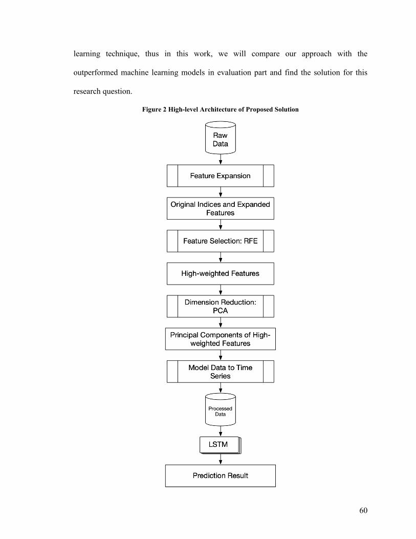
60
learning technique, thus in this work, we will compare our approach with the
outperformed machine learning models in evaluation part and find the solution for this
research question.
Figure 2 High-level Architecture of Proposed Solution

61
4.2 Technical Background – Technical Indices
In this section, we elaborate the most commonly used technical indices that conclude
from related works.
When building the model, most of the previous works illustrated their technical indices.
We found 15 the most frequent indices. The indices definitions refer to the appendix of
related work (Hsu, 2013).
1) Stochastic indicator K
The n-day stochastic indicator K is defined as:
𝐾_𝑛𝑖 =2
3× 𝐾_𝑛𝑖−1 +
1
3×𝐶𝑃𝑖 − 𝐿𝑃_𝑛𝑖𝐻𝑃_𝑛𝑖
× 100
Note the highest price in previous n days as HP_ni, and LP_ni as the lowest price in
previous n days. CPi is the closing price of day i.
2) Stochastic indicator D
The n-day stochastic indicator D
𝐷_𝑛𝑖 =2
3× 𝐷_𝑛(𝑖−1) +
1
3× 𝐾_𝑛𝑖
Where K_ni is the n-day stochastic indicator K of day i.
3) Williams overbought/oversold index
The n-day Williams overbought/oversold index is a momentum indicator that measures
overbought and oversold levels.
𝑊𝑀𝑆%𝑅_𝑛𝑖 =𝐻𝑃_𝑛𝑖 − 𝐶𝑃_𝑛𝑖𝐻𝑃_𝑛𝑖 − 𝐿𝑃_𝑛𝑖
4) Commodity channel index
The commodity channel index is used to identify cyclical turns in commodities.
We define the typical price as the formula below:

62
𝑇𝑃𝑖 =𝐻𝑃𝑖 + 𝐿𝑃𝑖 + 𝐶𝑃𝑖
3
Then we calculate the n-day simple moving average of the typical price:
𝑆𝑀𝐴𝑇𝑃_𝑛𝑖 =∑ 𝑇𝑃𝑗𝑖𝑗=𝑖−𝑛−1
𝑛
And the n-day mean deviation is noted by MD_n:
𝑀𝐷_𝑛𝑖 =∑ |𝑇𝑃𝑗 − 𝑆𝑀𝐴𝑇𝑃_𝑛𝑖|𝑖𝑗=𝑖−𝑛−1
𝑛
The n-day commodity channel index is calculated as:
𝐶𝐶𝐼_𝑛𝑖 =𝑇𝑃𝑖 − 𝑆𝑀𝐴𝑇𝑃_𝑛𝑖0.015 × 𝑀𝐷_𝑛𝑖
5) Relative strength index
The relative strength index is a momentum oscillator that compares the magnitude of
recent gains to the magnitude of recent losses.
𝐺𝑖 = {𝐶𝑃𝑖 − 𝐶𝑃𝑖−1, 𝑖𝑓 𝐶𝑃𝑖 > 𝐶𝑃𝑖−1 0 , 𝑜𝑡ℎ𝑒𝑟𝑤𝑖𝑠𝑒
6) Moving average convergence/divergence
The moving average convergence/divergence is a momentum indicator that shows the
relationship between two moving averages.
First step is to calculate the demand index (DI):
𝐷𝐼𝑖 = (𝐻𝑃𝑖 + 𝐿𝑃𝑖 + 2 × 𝐶𝑃𝑖)/4
We also need to calculate the 12-day and 26-day exponential moving average:
𝐸𝑀𝐴_12𝑖 =11
13× 𝐸𝑀𝐴_12𝑖−1 +
2
13× 𝐷𝐼𝑖
And
𝐸𝑀𝐴_26𝑖 =25
27× 𝐸𝑀𝐴_26𝑖−1 +
2
27× 𝐷𝐼𝑖

63
Hence, we use DIFi to indicate the difference between EMA_12 and EMA_26:
𝐷𝐼𝐹𝑖 = 𝐸𝑀𝐴_12𝑖 − 𝐸𝑀𝐴_26𝑖
The MACDi is calculated as below:
𝑀𝐴𝐶𝐷𝑖 =8
10× 𝑀𝐴𝐶𝐷𝑖−1 +
2
10× 𝐷𝐼𝐹𝑖
7) 10-day moving average
The 10-day moving average is the mean price of the futures over the most recent 10 days
and is calculated by:
𝑀𝐴_10𝑖 =∑ 𝐶𝑃𝑗𝑖𝑗=𝑖−9
10
8) Momentum
Momentum measures change in stock price over last n days
𝑀𝑇𝑀𝑖 =𝐶𝑃𝑖𝐶𝑃𝑖−𝑛
× 100
9) Rate of Change
The n-day rate of change measures the percent changes of the current price relative to the
price of n days ago and is calculated by:
𝑅𝑂𝐶_𝑛𝑖 =𝐶𝑃𝑖 − 𝐶𝑃𝑖−𝑛𝐶𝑃𝑖−𝑛
× 100
10) Psychological line
The psychological line is a volatility indicator based on the number of time intervals that
the market was up during the preceding period and is calculated by:
𝑃𝑆𝑌_𝑛𝑖 =𝑇𝐷𝑈_𝑛𝑖𝑛
× 100%
The TDU_ni is the total number of days that has price rises in previous n days.
11) AR

64
n-day A ratio means the n-day buying/selling momentum indicator which is calculated as:
𝐴𝑅_𝑛𝑖 =∑ (𝐻𝑃𝑗 −𝑂𝑃𝑗)𝑖𝑗=𝑖−𝑛−1
∑ (𝑂𝑃𝑗 − 𝐿𝑃𝑗)𝑖𝑗=𝑖−𝑛−1
12) BR
n-day B ratio means the n-day buying/selling willingness indicator and is defined as:
𝐵𝑅_𝑛𝑖 =∑ (𝐻𝑃𝑗 − 𝑂𝑃𝑗−1)𝑖𝑗=𝑖−𝑛−1
∑ (𝑂𝑃𝑗−1 − 𝐿𝑃𝑗)𝑖𝑗=𝑖−𝑛−1
13) Volume ratio
The n-day volume ratio is calculated by:
𝑉𝑅_𝑛𝑖 =𝑇𝑉𝑈_𝑛𝑖 − 𝑇𝑉𝐹_𝑛𝑖/2
𝑇𝑉𝐷_𝑛𝑖 − 𝑇𝑉𝐹_𝑛𝑖/2× 100%
Where the TVU represents the total trade volumes of stock price rising, and TVD is the
total trade volumes of stock prices falling, TVF represents the total trade volumes of
stock prices holding in previous n days.
14) Accumulation/distribution oscillator
𝐴𝐷𝑖 =𝐻𝑃𝑖 − 𝐶𝑃𝑖−1𝐻𝑃𝑖 − 𝐿𝑃𝑖
15) 5-day bias
The 5-day bias is the deviation between the closing price and the 5-day moving average
MA_5
𝐵𝐼𝐴𝑆_5𝑖 =𝐶𝑃𝑖 −𝑀𝐴_5𝑖𝑀𝐴_5𝑖
4.3 Proposed Solution
The high-level architecture of our proposed solution could be separated into three parts.
First is the feature selection part, guarantee the selected features are all effective. Second,

65
we look into the data and perform the dimensionality reduction. And the last part which is
the main contribution of our work is to build a prediction model of target stocks.
There are ways to classify different categories of stocks. Some investors prefer long-term
investment, while others show more interest in short-term investment. It is common to
see the stock-related company report shows an average performance, while the stock
price is increasing drastically; this is one of the phenomena that indicate the stock price
prediction has no fixed rules, thus find effective features before train the data model is
necessary.
In this project, we focus on short-term price trend prediction.
Currently, we only have the raw data with no labels; the very first step is to label the data.
We mark the price trend by comparing the current closing price with the closing price of
n trading days ago, the range of n is from 1 to 10 since our research is focusing on the
short-term. If the price trend goes up, we mark it as 1 or mark as 0 in the opposite case.
To be more specified, we use the indices from the indices of n−1th day to predict the
price trend of the nth day.
According to the previous works, some researchers who applied both financial domain
knowledge and technical methods on stock data were using rules to filter the high-quality
stocks. We referred to their works and exploited their rules to contribute to our feature
extension design.
However, to ensure the best performance of the prediction model, we will look into the
data first. There are a large number of features in the raw data; if we involve all the
features into our consideration, it will not only drastically increase the computational
complexity but will also cause side effects if we would like to perform unsupervised

66
learning in further research. So we leverage the recursive feature elimination (RFE) to
ensure all the selected features are effective.
Since we found most of the previous works in the technical domain were analyzing all
the stocks, while in the financial domain, researchers prefer to analyse the specific
scenario of investment, to fill the gap between the two domains, we decide to apply a
feature extension based on the findings we gathered from the financial domain before we
start the RFE procedure.
Since we plan to model the data into time series, the number of the features, the more
complex the training procedure will be. So, we will leverage the dimensionality reduction
by using randomized PCA at the beginning of our proposed solution architecture.
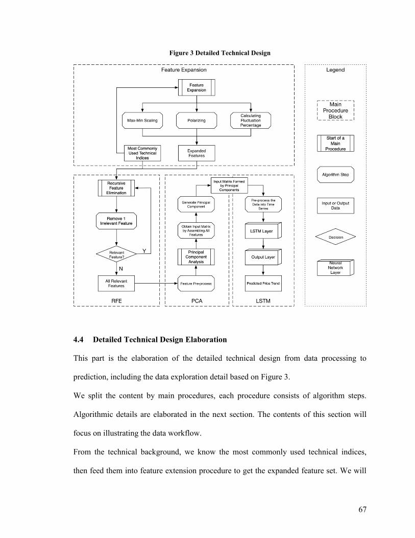
67
Figure 3 Detailed Technical Design
4.4 Detailed Technical Design Elaboration
This part is the elaboration of the detailed technical design from data processing to
prediction, including the data exploration detail based on Figure 3.
We split the content by main procedures, each procedure consists of algorithm steps.
Algorithmic details are elaborated in the next section. The contents of this section will
focus on illustrating the data workflow.
From the technical background, we know the most commonly used technical indices,
then feed them into feature extension procedure to get the expanded feature set. We will

68
select the most effective i features from the expanded feature set. Then we will feed the
data with i selected features into PCA algorithm to reduce the dimension into j features.
After we get the best combination of i and j, we process the data into finalized the feature
set and feed them into the LSTM model to get the price trend prediction result.
The novelty of our proposed solution is that we will not only apply the technical method
on raw data but also apply the feature extension that used among stock market investors.
4.4.1 Feature Extension
The first main procedure in Figure 3 is Feature extension. In this block, the input data is
the most commonly used technical indices concluded from related works.
The three feature extension methods are max-min scaling, polarizing, and calculating
fluctuation percentage. Be aware that not all the technical indices are applicable for all
three of the feature extension methods; this procedure only applies the meaningful
extension methods on technical indices. The technical indices calculation formulas are
elaborated in the Technical Background section; we choose the meaningful extension
methods according to how the indices calculated.
The technical indices and the corresponding feature extension methods are illustrated in
Table 17.
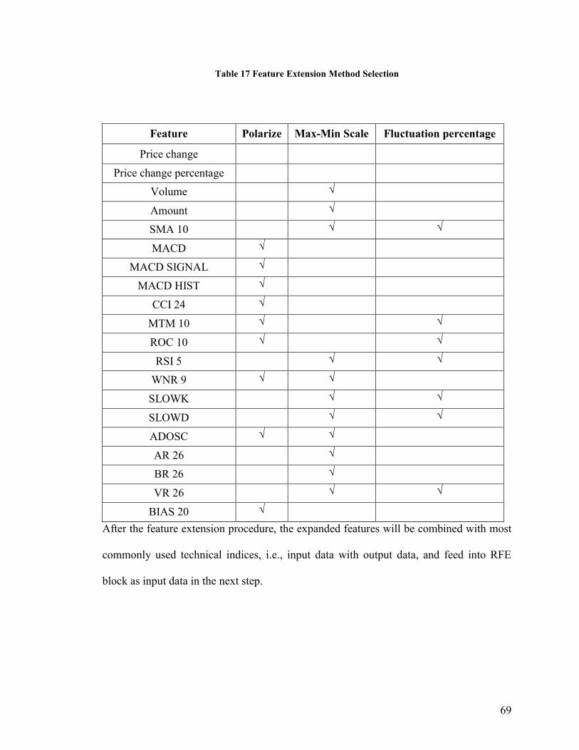
69
Table 17 Feature Extension Method Selection
After the feature extension procedure, the expanded features will be combined with most
commonly used technical indices, i.e., input data with output data, and feed into RFE
block as input data in the next step.
Feature Polarize Max-Min Scale Fluctuation percentage
Price change
Price change percentage
Volume √
Amount √
SMA 10 √ √
MACD √
MACD SIGNAL √
MACD HIST √
CCI 24 √
MTM 10 √ √
ROC 10 √ √
RSI 5 √ √
WNR 9 √ √
SLOWK √ √
SLOWD √ √
ADOSC √ √
AR 26 √
BR 26 √
VR 26 √ √
BIAS 20 √
70
4.4.2 Recursive Feature Elimination
After the feature extension above, we explore the most effective i features by using
Recursive Feature Elimination (RFE) algorithm. We estimate all the features by two
attributes, coefficient and feature importance. We also limit the features that remove from
the pool by one, which means we will remove one feature at each step and retain all the
relevant features.
Then the output of RFE block will be the input of the next step, which refers to PCA.
4.4.3 Principal Component Analysis
The very first step before leverage PCA is features pre-process. Because some of the
features after RFE are percentage data, while others are very large numbers, i.e. the
output from RFE are in different units. It will affect the principal component extraction
result. Thus, before feeding the data into PCA algorithm, a feature pre-processing is
necessary. We also illustrate the effectiveness and methods comparison in evaluation
section.
After performing feature pre-processing, the next step is to feed the processed data with
selected i features into PCA algorithm to reduce the feature matrix scale into j features.
This step is to retain as many effective features as possible and meanwhile eliminate the
computational complexity of training the model.
This research work also evaluates the best combination of i and j which has relatively
better prediction accuracy, meanwhile, cuts the computational consumption. The result
can be found in the evaluation section as well.
After the PCA step, the system will get a reshaped matrix with j columns.
71
4.4.4 Long Short-Term Memory
PCA reduced the scale of input data, while the data pre-processing is mandatory before
feeding the data into LSTM layer.
The reason of adding the data pre-processing step before LSTM model is that the input
matrix formed by principal components has no time steps. While one of the most
important parameters of training an LSTM is the number of time steps. Hence, we have
to model the matrix into corresponding time steps as for both training and testing dataset.
After performing the data pre-processing part, the last step is to feed the training data into
LSTM, and evaluate the performance using testing data.
As a variant neural network of RNN, even with one LSTM layer, the NN structure is still
a deep neural network since it can process sequential data and memorizes its hidden
states through time. An LSTM layer is composed of one or more LSTM units, an LSTM
unit consists of cells and gates to perform classification and prediction based on time
series data.
The LSTM structure is formed by two layers. Input dimension is determined by j after
PCA algorithm. The first layer is the input LSTM layer and the second layer is the output
layer.
The final output will be 0 or 1 indicates if the stock price trend prediction result is going
down or going up, as a supporting suggestion for the investors to perform the next
investment decision.

72
4.5 Design Discussion
Feature extension is one of the novelties of our proposed price trend predicting system. In
feature extension procedure, we use technical indices collaborate with the heuristic
processing methods learned from investors, which fills the gap between financial research
area and technical research area.
Since we proposed a system of price trend prediction, feature engineering is extremely
important to the final prediction result. Not only the feature extension method is helpful
to guarantee we do not miss the potentially correlated feature, but also feature selection
method is necessary for pooling the effective features. The more irrelevant features are
fed into the model, the more noise would be introduced. Each main procedure is carefully
considered contributing to the whole system design.
Besides feature engineering part, we also leverage LSTM, the state-of-the-art deep
learning method for time-series prediction, which guarantees the prediction model can
capture both complex hidden pattern and the time-series related pattern.
It is known that training cost of deep learning models is expansive in both time and
hardware aspects; another advantage of our system design is the optimization
procedure—PCA. It can retain the principal components of the features while reducing
the scale of the feature matrix, thus help the system to save the training cost of processing
the large time-series feature matrix.

73
4.6 Algorithm Elaboration
We elaborate the algorithm design in this part. Different from the previous section, this
section comprehensively explains the algorithms we exploit in perspectives of
terminologies, parameters, as well as optimizers.
From the legend on the right side of Figure 3, we note the algorithm steps as octagons, all
of them can be found in this algorithm elaboration section.
Before dive deep into the algorithm steps, here is the brief introduction of data pre-
processing: since we will go through the supervised learning algorithms, we also need to
program the ground truth. The ground truth of this project is programmed by comparing
the closing price of current trading date with the closing price of the previous trading date
the users want to compare with. Label the price increase as 1, else the ground truth will
be labeled as 0. Because this research work is not only focused on predicting price trend
of a specific period of time but short-term in general, the ground truth processing is
according to a range of trading days. While the algorithms will not change with the
prediction term length, we can regard the term length as a parameter.
The algorithmic detail is elaborated, respectively, the first algorithm is the hybrid feature
engineering part for preparing high-quality training and testing data. It corresponds to the
Feature extension, RFE and PCA blocks in Figure 3. And the second algorithm is the
LSTM procedure block, including time-series data pre-processing, NN constructing,
training, and testing.

74
4.6.1 Algorithm 1: Short-term Stock Market Price Trend Prediction - Hybrid
Feature Engineering Using FE+RFE+PCA
The function FE () is corresponding to the feature extension block.
For the feature extension procedure, we apply three different processing methods to
translate the findings from the financial domain to a technical module in our system
design. While not all the indices are applicable for expanding, we only choose the proper
method(s) for certain features to perform the feature extension according to Table 17.
Normalize method preserves the relative frequencies of the terms, and transform the
technical indices into the range of [0, 1]. Polarize is a method often used by real world
investors, sometimes they prefer to consider if the technical index value is above or
below zero, we program some of the features using polarize method and prepare for RFE.
Max min scale is a transform method often used as an alternative to zero mean and unit
variance scaling. The fourth method is fluctuation percentage, we transform the technical
indices fluctuation percentage into the range of [-1, 1].
The function RFE () in the first algorithm refers to recursive feature elimination. Before
we perform the training data scale reduction, we will have to make sure that the features
we selected are effective. Ineffective features will not only drag down the classification
precision, but also add more computational complexity. For the feature selection part, we
choose recursive feature elimination (RFE).
As (Weng et al., 2018) introduced, the RFE algorithm can be split into ranking algorithm,
resampling and external validation.
For the ranking algorithm, it fits the model to the features and rank by the importance to
the model. We set the parameter to retain i numbers of features, and at each iteration of
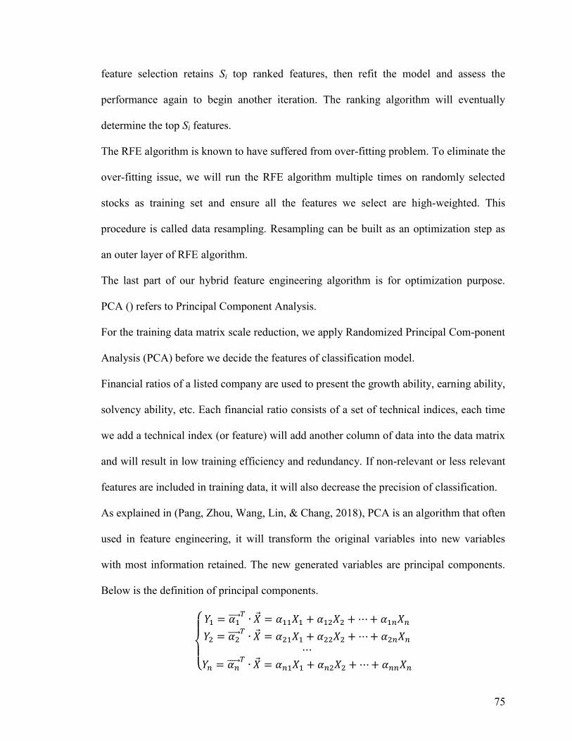
75
feature selection retains Si top ranked features, then refit the model and assess the
performance again to begin another iteration. The ranking algorithm will eventually
determine the top Si features.
The RFE algorithm is known to have suffered from over-fitting problem. To eliminate the
over-fitting issue, we will run the RFE algorithm multiple times on randomly selected
stocks as training set and ensure all the features we select are high-weighted. This
procedure is called data resampling. Resampling can be built as an optimization step as
an outer layer of RFE algorithm.
The last part of our hybrid feature engineering algorithm is for optimization purpose.
PCA () refers to Principal Component Analysis.
For the training data matrix scale reduction, we apply Randomized Principal Component
Analysis (PCA) before we decide the features of classification model.
Financial ratios of a listed company are used to present the growth ability, earning ability,
solvency ability, etc. Each financial ratio consists of a set of technical indices, each time
we add a technical index (or feature) will add another column of data into the data matrix
and will result in low training efficiency and redundancy. If non-relevant or less relevant
features are included in training data, it will also decrease the precision of classification.
As explained in (Pang, Zhou, Wang, Lin, & Chang, 2018), PCA is an algorithm that often
used in feature engineering, it will transform the original variables into new variables
with most information retained. The new generated variables are principal components.
Below is the definition of principal components.
{
𝑌1 = 𝛼1⃗⃗⃗⃗
𝑇∙ 𝑋 = 𝛼11𝑋1 + 𝛼12𝑋2 +⋯+ 𝛼1𝑛𝑋𝑛
𝑌2 = 𝛼2⃗⃗⃗⃗ 𝑇∙ 𝑋 = 𝛼21𝑋1 + 𝛼22𝑋2 +⋯+ 𝛼2𝑛𝑋𝑛
⋯
𝑌𝑛 = 𝛼𝑛⃗⃗ ⃗⃗ 𝑇∙ 𝑋 = 𝛼𝑛1𝑋1 + 𝛼𝑛2𝑋2 +⋯+ 𝛼𝑛𝑛𝑋𝑛

76
Xi is the original variable, Yi is the principal component and 𝛼 𝑖 is the coefficient vector.
By minimizing 𝑉𝑎𝑟(𝑌𝑖) with the constraint conditions of 𝛼1⃗⃗⃗⃗ 𝑇∙ 𝑋 = 1 and 𝐶𝑜𝑣(𝑌𝑖 , 𝑌𝑗) =
𝛼𝑖⃗⃗ ⃗𝑇∙ 𝛼𝑖⃗⃗ ⃗ = 0, 𝑗 = 1,2,⋯ , 𝑖 − 1, where ∑ = (𝜎𝑖𝑗)𝑛×𝑛 is the covariance matrix of 𝑋 .
The next step is the selection of principal components. The covariance matrix of 𝑋 =
(𝑋1, 𝑋2,⋯𝑋𝑛)3∑ = (𝜎𝑖𝑗)𝑛×𝑛 , is a symmetric non-negative definite matrix. Thus, this
matrix has n characteristic roots λ1, λ2, ..., λn and n characteristic vectors.
All the roots λ ≥ 0, besides, the orthogonal unit eigenvectors are 𝑒1⃗⃗ ⃗, 𝑒2⃗⃗ ⃗, ⋯ , 𝑒𝑛⃗⃗⃗⃗ . The ith
principal component of X1,X
2,...,X
ncan be illustrated as:
𝑌𝑖 = 𝑒𝑖1𝑋1 + 𝑒𝑖2𝑋2 +⋯+ 𝑒𝑖𝑛𝑋𝑛, 𝑖 = 1,2,⋯ , 𝑛
With 𝐶𝑜𝑣(𝑌𝑖, 𝑌𝑗) = 𝑒𝑖⃗⃗ 𝑇∙ ∑ 𝑒𝑖⃗⃗ = 0, 𝑖 ≠ 𝑗 and 𝑉𝑎𝑟(𝑌𝑖) = 𝑒𝑖⃗⃗
𝑇∙ ∑ 𝑒𝑖⃗⃗ = λ𝑖 , the first
accumulated contribution rate of principal components p is noted as:
𝐴𝐶𝑅(𝑝) =∑ λ𝑖/∑ λ𝑖𝑛
𝑖=1
𝑝
𝑖=1
The above equation represents the explanation power of principal components extracted
by PCA method for original data. If an ACR is below 85%, the PCA method would be
unsuitable due to a loss of original information. Because the covariance matrix is
sensitive to the order of magnitudes of data, there should be a data standardize procedure
before performing the PCA. The commonly used standardize methods are mean-
standardization and normal-standardization and could be noted as below respectively:
Mean-standardization: 𝑋𝑖𝑗∗ = 𝑋𝑖𝑗/𝑋�̅�, which 𝑋�̅� represents the mean value.
Normal-standardization: 𝑋𝑖𝑗∗ = (𝑋𝑖𝑗 − 𝑋�̅�)/𝑠𝑗 , which 𝑋�̅� represents the mean
value, and 𝑠𝑗 is the standard deviation.

77
The array fe_array is defined according to the Table 17, row number maps to the features,
column 0, 1, 2, 3 note for the extension methods of normalize, polarize, max min scale
and fluctuation percentage respectively. Then we fill in the values for the array by the
rule where 0 stands for no necessity to expand and 1 for features need to apply the
corresponding extension methods.
The final algorithm of data preprocessing using RFE and PCA can be illustrated as
Algorithm 1.
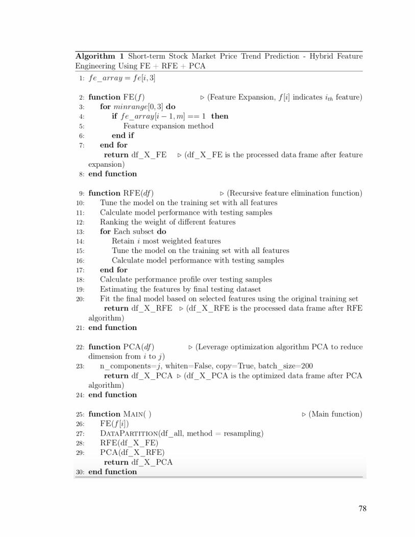
78

79
4.6.2 Algorithm 2: Price Trend Prediction Model Using LSTM
After the principal component extraction, we will get the scale-reduced matrix, which
means i most effective features are converted into j principal components for training the
prediction model.
We exploit an LSTM model, and added a conversion procedure for our stock price
dataset. The detail algorithm design is illustrated in Alg 2.
The function TIMESERIESCONVERSION () converts the principal components matrix
into time series by shifting the input data frame according to the number of time steps i.e.
term length in this project. The processed dataset consists of input sequence and forecast
sequence. In this project, the parameter of lag is 1, because the model is detecting the
pattern of features fluctuation in daily basis. Meanwhile, the NTIMESTEPS is varied from
1 trading day to 10 trading days.
We omit the function description of DATAPARTITION (), FITMODEL (), EVALUATE
MODE () since the functions above are regular steps without customization.
The NN structure design, optimizer decision and other parameters are illustrated in
function MODELCOMPILE ().

80

81
4.7 Use Case of Proposed Solution
In this section, we elaborate the use case of our proposed solution, i.e., how we
implement the proposed solution as an application.
The major purpose of this use case is to build a lite, easy-to-access application;
meanwhile, we prefer an all-python implementation to retain the consistency of system
components.
The overall architecture of the use case design is illustrated in Figure 4.
The application consists of three layers: data collection & storage, data processing,
graphical user interface (GUI).
To achieve the purpose of building an easy-to-access application, we prefer to build a
web application, so that users can access the application anywhere anytime with the URL.
The first layer is the basic layer of this web application, data collection & storage. For the
demo application, we only apply the code of data storage part, while it would be easy to
slightly modify the data collection code and collect daily stock data from Tushare API
then store to the database.
The second layer is data processing. In this layer, deploy the python codes from Chapter
4.6.
The third layer is the graphical user interface for user input and result output. Demo
version web application has a GUI for users to fill in the stock ID, trade date, prediction
time range, with an output of the prediction result.
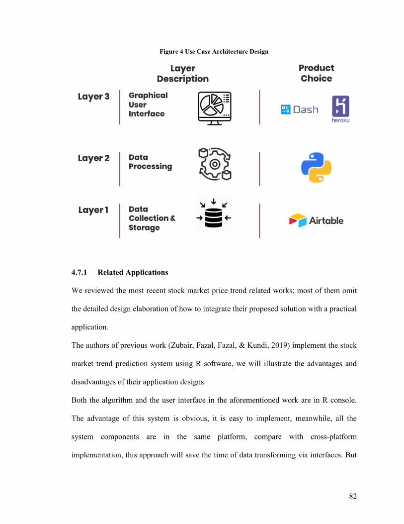
82
Figure 4 Use Case Architecture Design
4.7.1 Related Applications
We reviewed the most recent stock market price trend related works; most of them omit
the detailed design elaboration of how to integrate their proposed solution with a practical
application.
The authors of previous work (Zubair, Fazal, Fazal, & Kundi, 2019) implement the stock
market trend prediction system using R software, we will illustrate the advantages and
disadvantages of their application designs.
Both the algorithm and the user interface in the aforementioned work are in R console.
The advantage of this system is obvious, it is easy to implement, meanwhile, all the
system components are in the same platform, compare with cross-platform
implementation, this approach will save the time of data transforming via interfaces. But
83
implement all the components within R console also causes some weaknesses in the
meantime. The user interface of their recommendation system is difficult to understand
for the users who are not familiar with R software, and it is impossible to access their
recommend system without all the algorithms and components being deployed locally.
4.7.2 Application Deployment and GUI Explanation
This section illustrates the application decision-making and the reasons for choosing
certain products.
For data storage, we choose Airtable (Airtable, 2019) as it can store different types of
data, even image. In the start-up stage, it would be more flexible if we plan to add more
types of data into the database to further extend the application functionalities. For
instance, if we plan to construct a CNN model to analyze the price trend line graphs, we
can get the training data straight from the same database without linking the data from a
different source. Another advantage of using Airtable as a database is that the data
structure of Airtable is flexible. We can regard Airtable as a No-SQL database with a
comprehensive GUI since the data are in json format. The flexibility of Airtable provides
us the convenience to test the data structure, and it is the first step of making the decision
of dataset architecture for a mature product.
We choose Heroku (Heroku, 2019) to deploy the web application, and use Plotly Dash
(Dash, 2019) to develop the user interface layer.
Plotly Dash is a python-based library, it can integrate very well with Pandas data frame.
For integrating Airtable with Plotly Dash, we also exploit a python library called airtable-
84
python-wrapper. And by using HTML, CSS and JavaScript, user can easily style the web
application via the normal procedure for web page development.
The Figure 5 is the GUI of our use case web application.
First of all, select the start date of the price trend prediction period, then select the
prediction time range from three options: every other day, weekly, bi-weekly. Then fill in
the stock ID of which the user would like to predict and click the Submit button.
The result will show in the Prediction Result section.
4.7.3 Potential of the Use Case
This section is a discussion about the potential of this use case. From the current available
function, we can see, actually, there is a high potential in extending the application
functionalities.
Since Plotly Dash is a powerful library for data visualization; meanwhile, data
visualization also plays an important role in stock analysis. We can add line graphs for
stock price and technical indices in the future as previous products since our web
application has already embedded the price trend prediction functionality which distinct
from other existed stock market analysis products.
Moreover, it is also possible to upgrade the data collection and storage layer. As we
mentioned in previous section, flexibility is the major reason that we choose Airtable as
the database product, because our product is still in the start-up stage, the data structure is
not maturely defined yet. While as the application develops, it would be better to store
the stock market price data into a relational database. Heroku also offers the Postgres
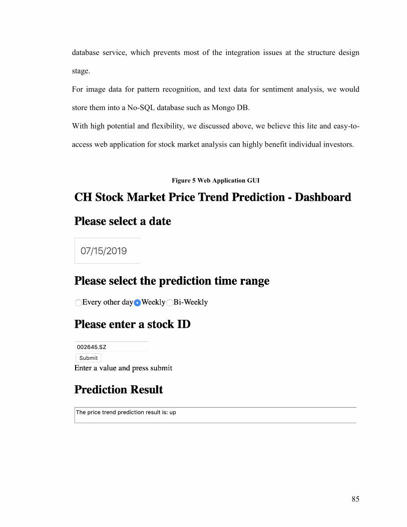
85
database service, which prevents most of the integration issues at the structure design
stage.
For image data for pattern recognition, and text data for sentiment analysis, we would
store them into a No-SQL database such as Mongo DB.
With high potential and flexibility, we discussed above, we believe this lite and easy-to-
access web application for stock market analysis can highly benefit individual investors.
Figure 5 Web Application GUI

86
Chapter 5: Evaluation
Some procedures impact the efficiency but do not affect the accuracy or precision and
vice-versa, while other procedures may affect both efficiency and prediction result. To
fully evaluate our algorithm design we structure the evaluation part by main procedures,
and evaluate how each procedure affects the algorithm performance.
We evaluated the entire algorithm on a macOS laptop with 2.2 GHz Intel Core i7
processor, embedded 16 GB 1600 MHz DDR3 memory.
In this section, we introduce the evaluation part in detail. In the implementation part, we
know that we have expanded 20 features into 54 features, while we retain 30 features that
are the most effective. In this section, we record the evaluation detail of feature selection
part.
The contents of this section are split into three main parts for each step in implementation.
While before the detail illustration of evaluation procedures, we begin this part with
introducing how we split the dataset. Test procedure including two parts, one testing
dataset is for feature selection and another one is for models testing. We note the feature
selection dataset and model testing dataset as DS_test_f and DS_test_m, respectively.
We randomly select two thirds of the stock data by stock ID for RFE training and notes
the dataset as DS_train_f, all the data consist of full technical indices and expanded
features throughout 2018. The estimator of RFE algorithm is SVR with linear kernels.
We rank the 54 features by voting and get 30 effective features then process them using
PCA algorithm to perform dimension reduction and reduce the features into 20 principal
components. The rest of stock data forms the testing dataset DS_test_f to validate the
effectiveness of principal components we extracted from selected features.

87
We reform all the data from 2018 as the training dataset of the data model and noted as
DS_train_m.
The model testing dataset DS_test_m consists of the first 3 months of data in 2019, which
has no overlap with the dataset we exploited in previous steps. This approach is to
prevent the hidden problem caused by overfitting.
5.1 Term Length
To build an efficient prediction model, instead of the approach of modeling the data to
time series, we determined to use one day ahead indices data to predict the price trend of
the next day.
We tested the RFE algorithm on a range of short-term from one day to two weeks (ten
trading days), to evaluate how commonly used technical indices correlated to the price
trend.
For evaluating the prediction term length, we fully expanded the features as the Table 17
above, and feed them to RFE.
During the test, we found that different length of term has a different level of sensitive-
ness to the same indices set.
We get the close price of the first trading date, and compare it with the close price of the
n_th trading date. Since we are predicting the price trend, we do not consider the term
lengths if the cross-validation score is below 0.5. And after the test, as we can see from
the Fig 4, there are three term lengths that are most sensitive to the indices we selected
from the related works. They are n = {2, 5, 10}, which indicates that price trend
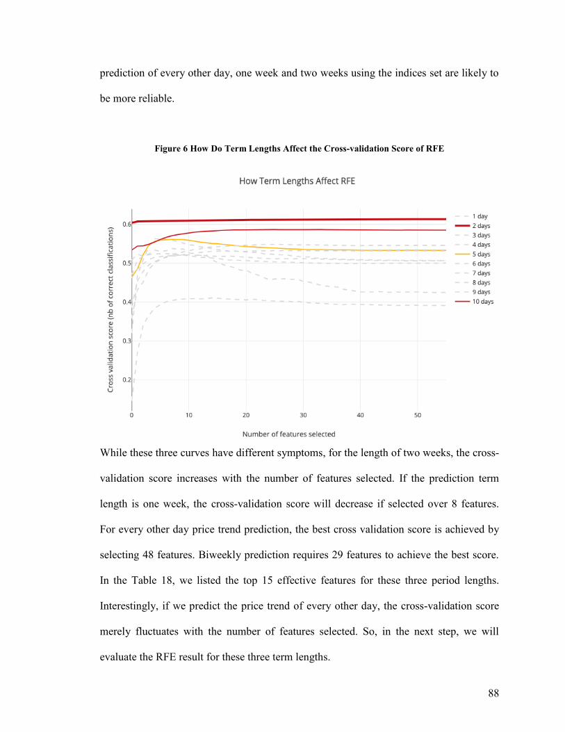
88
prediction of every other day, one week and two weeks using the indices set are likely to
be more reliable.
Figure 6 How Do Term Lengths Affect the Cross-validation Score of RFE
While these three curves have different symptoms, for the length of two weeks, the cross-
validation score increases with the number of features selected. If the prediction term
length is one week, the cross-validation score will decrease if selected over 8 features.
For every other day price trend prediction, the best cross validation score is achieved by
selecting 48 features. Biweekly prediction requires 29 features to achieve the best score.
In the Table 18, we listed the top 15 effective features for these three period lengths.
Interestingly, if we predict the price trend of every other day, the cross-validation score
merely fluctuates with the number of features selected. So, in the next step, we will
evaluate the RFE result for these three term lengths.
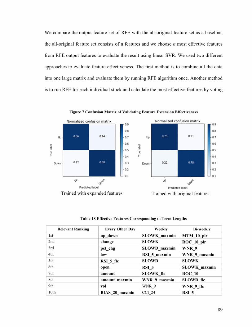
89
We compare the output feature set of RFE with the all-original feature set as a baseline,
the all-original feature set consists of n features and we choose n most effective features
from RFE output features to evaluate the result using linear SVR. We used two different
approaches to evaluate feature effectiveness. The first method is to combine all the data
into one large matrix and evaluate them by running RFE algorithm once. Another method
is to run RFE for each individual stock and calculate the most effective features by voting.
Figure 7 Confusion Matrix of Validating Feature Extension Effectiveness
Table 18 Effective Features Corresponding to Term Lengths
Relevant Ranking Every Other Day Weekly Bi-weekly
1st up_down SLOWK_maxmin MTM_10_plr
2nd change SLOWK ROC_10_plr
3rd pct_chg SLOWD_maxmin WNR_9
4th low RSI_5_maxmin WNR_9_maxmin
5th RSI_5_flc SLOWD SLOWK
6th open RSI_5 SLOWK_maxmin
7th amount SLOWK_flc ROC_10
8th amount_maxmin WNR_9_maxmin SLOWD_flc
9th vol WNR_9 WNR_9_flc
10th BIAS_20_maxmin CCI_24 RSI_5
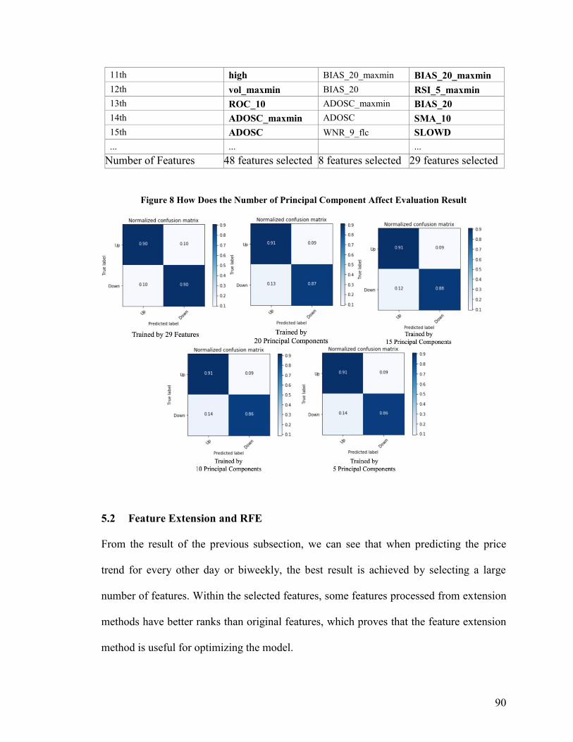
90
11th high BIAS_20_maxmin BIAS_20_maxmin
12th vol_maxmin BIAS_20 RSI_5_maxmin
13th ROC_10 ADOSC_maxmin BIAS_20
14th ADOSC_maxmin ADOSC SMA_10
15th ADOSC WNR_9_flc SLOWD
... ... ...
Number of Features
Selected
48 features selected 8 features selected 29 features selected
Figure 8 How Does the Number of Principal Component Affect Evaluation Result
5.2 Feature Extension and RFE
From the result of the previous subsection, we can see that when predicting the price
trend for every other day or biweekly, the best result is achieved by selecting a large
number of features. Within the selected features, some features processed from extension
methods have better ranks than original features, which proves that the feature extension
method is useful for optimizing the model.

91
The feature extension affects both precision and efficiency, while in this part, we only
discuss the precision aspect and leave efficiency part in the next step since PCA is the
most effective method for training efficiency optimization in our design. We involved an
evaluation of how feature extension affects RFE, and use the test result to measure the
improvement of involving feature extension.
In this subsection, we would test the effectiveness of feature extension: if polarize, max-
min scale and calculate fluctuation percentage works better than original technical indices.
The best case to leverage this test is the weekly prediction since it has the least effective
feature selected. From the result we got from the last section, we know the best cross-
validation score appears when selecting 8 features. The test consists of two steps, the first
step is to test the feature set formed by original features only, in this case, only SLOWK,
SLOWD, and RSI_5 are included. Next step is to test the feature set of all 8 features we
selected in the previous subsection. We leveraged the test by defining the simplest DNN
model with three layers.
The normalized confusion matrix of testing the two feature sets are illustrated in Figure 7.
The left one is the confusion matrix of the feature set with expanded features, and the
right one besides is the test result of using original features only.
Both precision of true positive and true negative has been improved by 7% and 10%
respectively, which proves that our feature extension method design is reasonably
effective.
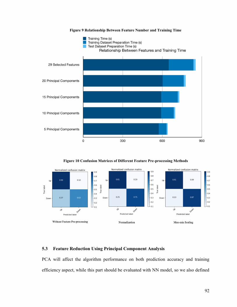
92
Figure 9 Relationship Between Feature Number and Training Time
Figure 10 Confusion Matrices of Different Feature Pre-processing Methods
5.3 Feature Reduction Using Principal Component Analysis
PCA will affect the algorithm performance on both prediction accuracy and training
efficiency aspect, while this part should be evaluated with NN model, so we also defined
93
a simplest DNN model with three layers as we used in the previous step to perform the
evaluation.
This part introduces the evaluation method and result of the optimization part of the
model from computational efficiency and accuracy impact perspectives.
Table 19 Relationship Between the Number of Principal Components and Training Efficiency
Number of
Features
Training Dataset
Preparation Time (s)
Test Dataset
Preparation Time (s)
Training
Time (s) Sum (s)
29 Selected
Features
187.46 16.30 648.53 852.29
20 Principal
Components
160.29 14.24 602.68 777.21
15 Principal
Components
125.20 12.18 591.93 729.31
10 Principal
Components
96.54 10.37 590.76 697.67
5 Principal
Components
59.37 8.22 572.88 640.47
Table 20 How Does the Number of Selected Features Affect the Prediction Accuracy
Number of
Selected
Features
5 Principal
Components
10 Principal
Components
15 Principal
Components
20 Principal
Components
29 Selected
Features
Accuracy 89.03% 89.35% 89.39% 89.30% 90.29%

94
In this section, we will choose bi-weekly prediction to perform a use case analysis, since
it has a smoothly increasing cross validation score curve, moreover, unlike every other
day prediction, it has excluded more than 20 ineffective features already. In the first step,
we select all 29 effective features and train the NN model without performing PCA. It
creates a baseline of the accuracy and training time for comparison. To evaluate the
accuracy and efficiency, we keep the number of principal component as 5, 10, 15, 20, 25.
The Table 19 recorded how number of features affect the model training efficiency, then
use the stack bar chart in Figure 9 to illustrate how PCA affect the training efficiency.
We also listed the confusion matrix of each test in Figure 8.
The stack bar chart shows that the overall time spends on training the model is decreasing
by the number of selected features, while the PCA method is significantly effective on
optimizing training dataset preparation. For the time spent on training stage, PCA is not
as effective as data preparation stage. While there is the possibility that the optimization
effect of PCA is not drastic enough because of the simple structure of NN model.
Table 20 indicates that the overall prediction accuracy is not drastically affected by
reducing the dimension. However, the accuracy could not fully support if the PCA has no
side effect to model prediction, so we looked into the confusion matrices of test results
95
Table 21 Accuracy and Efficiency Analysis on Feature Pre-processing Procedures
Feature Pre-
processing
Overall
Accuracy (%)
Training Dataset
Preparation Time
(s)
Testing Dataset
Preparation
Time(s)
Training Time
(s)
Sum
(s)
Max-min Scaling 89.30 160.28 14.24 602.68 777.20
Normalization 78.17 157.63 14.73 596.22 768.58
N/A 78.88 142.17 13.00 595.52 750.69
using different number of selected features. From Figure 8 we can conclude that PCA
does not have a severe negative impact on prediction precision. The true positive rate and
false positive rate are barely be affected, while the false negative and true negative rate
are influenced by 2% to 4%.
Besides evaluating how the number of selected features affects the training efficiency and
model performance, we also leveraged a test upon how data pre-processing procedures
affect the training procedure and predicting result. Normalizing and max-min scaling are
the most commonly seen data pre-procedure performed before PCA, since the measure
units of features are varied and it is said that it could increase the training efficiency
afterwards.
We leveraged another test on adding pre-procedures before extracting 20 principal
components from original dataset, and make the comparison in the aspects of time elapse
of training stage and prediction precision.
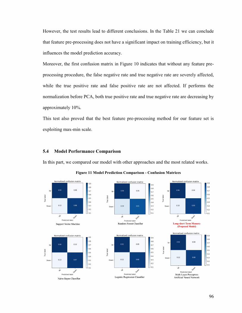
96
However, the test results lead to different conclusions. In the Table 21 we can conclude
that feature pre-processing does not have a significant impact on training efficiency, but it
influences the model prediction accuracy.
Moreover, the first confusion matrix in Figure 10 indicates that without any feature pre-
processing procedure, the false negative rate and true negative rate are severely affected,
while the true positive rate and false positive rate are not affected. If performs the
normalization before PCA, both true positive rate and true negative rate are decreasing by
approximately 10%.
This test also proved that the best feature pre-processing method for our feature set is
exploiting max-min scale.
5.4 Model Performance Comparison
In this part, we compared our model with other approaches and the most related works.
Figure 11 Model Prediction Comparison - Confusion Matrices
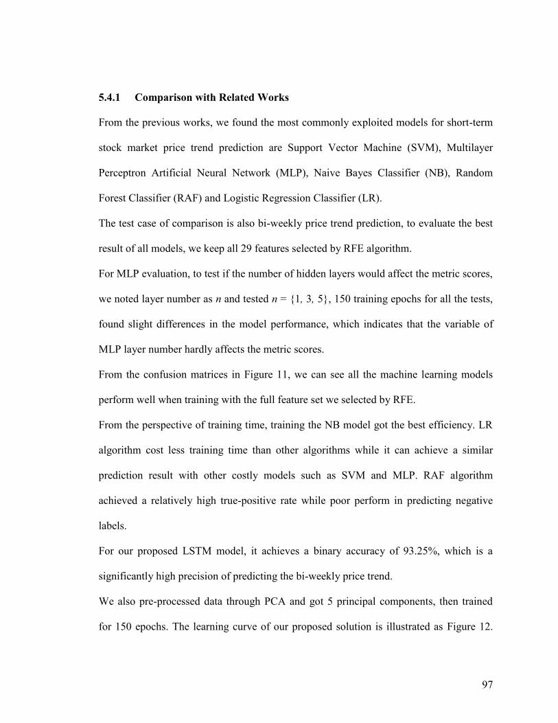
97
5.4.1 Comparison with Related Works
From the previous works, we found the most commonly exploited models for short-term
stock market price trend prediction are Support Vector Machine (SVM), Multilayer
Perceptron Artificial Neural Network (MLP), Naive Bayes Classifier (NB), Random
Forest Classifier (RAF) and Logistic Regression Classifier (LR).
The test case of comparison is also bi-weekly price trend prediction, to evaluate the best
result of all models, we keep all 29 features selected by RFE algorithm.
For MLP evaluation, to test if the number of hidden layers would affect the metric scores,
we noted layer number as n and tested n = {1, 3, 5}, 150 training epochs for all the tests,
found slight differences in the model performance, which indicates that the variable of
MLP layer number hardly affects the metric scores.
From the confusion matrices in Figure 11, we can see all the machine learning models
perform well when training with the full feature set we selected by RFE.
From the perspective of training time, training the NB model got the best efficiency. LR
algorithm cost less training time than other algorithms while it can achieve a similar
prediction result with other costly models such as SVM and MLP. RAF algorithm
achieved a relatively high true-positive rate while poor perform in predicting negative
labels.
For our proposed LSTM model, it achieves a binary accuracy of 93.25%, which is a
significantly high precision of predicting the bi-weekly price trend.
We also pre-processed data through PCA and got 5 principal components, then trained
for 150 epochs. The learning curve of our proposed solution is illustrated as Figure 12.
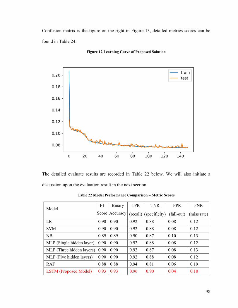
98
Confusion matrix is the figure on the right in Figure 13, detailed metrics scores can be
found in Table 24.
Figure 12 Learning Curve of Proposed Solution
The detailed evaluate results are recorded in Table 22 below. We will also initiate a
discussion upon the evaluation result in the next section.
Table 22 Model Performance Comparison – Metric Scores
Model F1
Score
Binary
Accuracy
TPR
(recall)
TNR
(specificity)
FPR
(fall-out)
FNR
(miss rate)
LR 0.90 0.90 0.92 0.88 0.08 0.12
SVM 0.90 0.90 0.92 0.88 0.08 0.12
NB 0.89 0.89 0.90 0.87 0.10 0.13
MLP (Single hidden layer) 0.90 0.90 0.92 0.88 0.08 0.12
MLP (Three hidden layers) 0.90 0.90 0.92 0.87 0.08 0.13
MLP (Five hidden layers) 0.90 0.90 0.92 0.88 0.08 0.12
RAF 0.88 0.88 0.94 0.81 0.06 0.19
LSTM (Proposed Model) 0.93 0.93 0.96 0.90 0.04 0.10
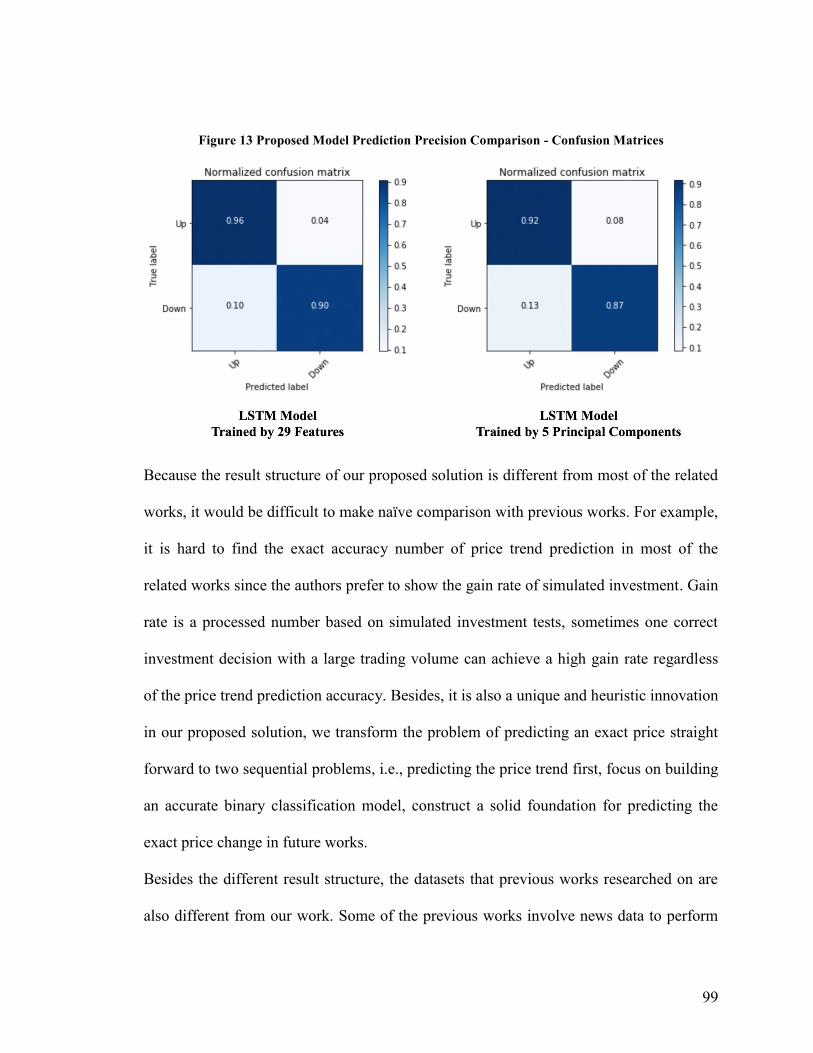
99
Figure 13 Proposed Model Prediction Precision Comparison - Confusion Matrices
Because the result structure of our proposed solution is different from most of the related
works, it would be difficult to make naïve comparison with previous works. For example,
it is hard to find the exact accuracy number of price trend prediction in most of the
related works since the authors prefer to show the gain rate of simulated investment. Gain
rate is a processed number based on simulated investment tests, sometimes one correct
investment decision with a large trading volume can achieve a high gain rate regardless
of the price trend prediction accuracy. Besides, it is also a unique and heuristic innovation
in our proposed solution, we transform the problem of predicting an exact price straight
forward to two sequential problems, i.e., predicting the price trend first, focus on building
an accurate binary classification model, construct a solid foundation for predicting the
exact price change in future works.
Besides the different result structure, the datasets that previous works researched on are
also different from our work. Some of the previous works involve news data to perform

100
sentiment analysis and exploit SE part as another system component to support their
prediction model.
The latest related work that can compare is (Zubair et al., 2019), the authors take multiple
r-square for model accuracy measurement. Multiple r-square is also called the coefficient
of determination, it shows the strength of predictor variables explaining the variation in
stock return (Nagar, Anurag; Hahsler, 2012). They used three datasets (KSE 100 Index,
Lucky Cement Stock, Engro Fertilizer Limited) to evaluate the proposed multiple
regression model, and achieved 95%, 89% and 97% respectively. Except for KSE 100
Index, the dataset choice in this related work is individual stocks; thus, we choose the
evaluation result of the first dataset of their proposed model.
We listed the leading stock price trend prediction model performance in Table 23, from
the comparable metrics, the metric scores of our proposed solution are generally better
than other related works. Instead of concluding arbitrarily that our proposed model
outperformed other models in related works, we first look into the dataset column of
Table 23. By looking into the dataset used by each work (Khaidem & Dey, 2016) only
trained and test their proposed solution on three individual stocks, which is difficult to
prove the generalization of their proposed model. (Ayo, 2014) leveraged analysis on the
stock data from New York Stock Exchange (NYSE), while the weakness is they only
performed analysis on closing price, which is a feature embedded with high noise.
(Zubair et al., 2019) trained their proposed model on both individual stocks and index
price, but as we have mentioned in the previous section, index price only consists of
limited number of features and stock IDs, which will further affect the model training
quality. For our proposed solution, we collected sufficient data from Chinese stock
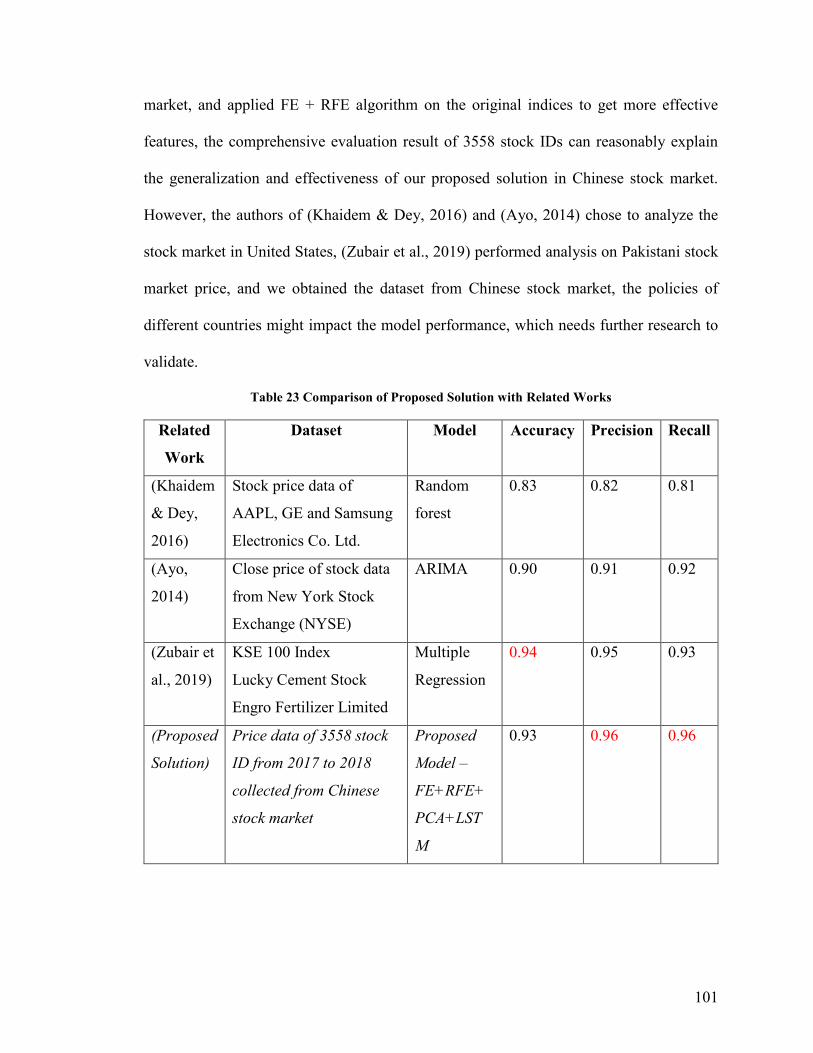
101
market, and applied FE + RFE algorithm on the original indices to get more effective
features, the comprehensive evaluation result of 3558 stock IDs can reasonably explain
the generalization and effectiveness of our proposed solution in Chinese stock market.
However, the authors of (Khaidem & Dey, 2016) and (Ayo, 2014) chose to analyze the
stock market in United States, (Zubair et al., 2019) performed analysis on Pakistani stock
market price, and we obtained the dataset from Chinese stock market, the policies of
different countries might impact the model performance, which needs further research to
validate.
Table 23 Comparison of Proposed Solution with Related Works
Related
Work
Dataset Model Accuracy Precision Recall
(Khaidem
& Dey,
2016)
Stock price data of
AAPL, GE and Samsung
Electronics Co. Ltd.
Random
forest
0.83 0.82 0.81
(Ayo,
2014)
Close price of stock data
from New York Stock
Exchange (NYSE)
ARIMA 0.90 0.91 0.92
(Zubair et
al., 2019)
KSE 100 Index
Lucky Cement Stock
Engro Fertilizer Limited
Multiple
Regression
0.94 0.95 0.93
(Proposed
Solution)
Price data of 3558 stock
ID from 2017 to 2018
collected from Chinese
stock market
Proposed
Model –
FE+RFE+
PCA+LST
M
0.93 0.96 0.96
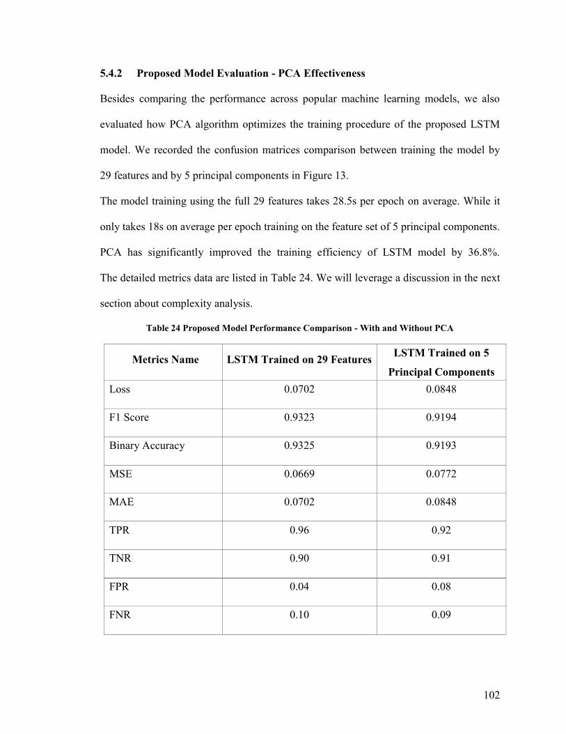
102
5.4.2 Proposed Model Evaluation - PCA Effectiveness
Besides comparing the performance across popular machine learning models, we also
evaluated how PCA algorithm optimizes the training procedure of the proposed LSTM
model. We recorded the confusion matrices comparison between training the model by
29 features and by 5 principal components in Figure 13.
The model training using the full 29 features takes 28.5s per epoch on average. While it
only takes 18s on average per epoch training on the feature set of 5 principal components.
PCA has significantly improved the training efficiency of LSTM model by 36.8%.
The detailed metrics data are listed in Table 24. We will leverage a discussion in the next
section about complexity analysis.
Table 24 Proposed Model Performance Comparison - With and Without PCA
Metrics Name LSTM Trained on 29 Features LSTM Trained on 5
Principal Components
Loss 0.0702 0.0848
F1 Score 0.9323 0.9194
Binary Accuracy 0.9325 0.9193
MSE 0.0669 0.0772
MAE 0.0702 0.0848
TPR 0.96 0.92
TNR 0.90 0.91
FPR 0.04 0.08
FNR 0.10 0.09

103
5.5 Discussions and Implications
In this section, we will discuss the findings from the results we got from the evaluations
above. The discussion contents are formed by the related findings and answers back to
the research questions.
5.5.1 RQ1: How does feature engineering benefit model prediction accuracy?
As we illustrated in the proposed solution part, the algorithm for feature engineering in
this project was RFE. The curves in Figure 6 obviously show that when the feature
number reaches a certain threshold, the cross-validation score will no longer increase and
would even drop with more features selected. The thresholds are varied from different
term lengths.
This finding shows that over selected features will only overload the hardware resources
and increasing training time but not contributes to the model prediction accuracy and
might have a negative impact on the prediction task.
From the confusion matrices of different model prediction precision in Figure 11 we can
also conclude that with a well-selected feature set, even a simple classifier such as Naive
Bayes Classifier can also achieve a relatively accurate prediction result. It also proved
that the feature engineering plays an important role in data preparation and model design
part.
5.5.2 RQ2: How do findings from financial domain benefit prediction model
design?

104
We translated the most helpful findings from financial domain into technical processing,
which could benefit our research project. We called this procedure as feature extension.
Table 18 records the top 15 features that selected by RFE after feature extension
procedures. From the effective features of three different time lengths, we can see that the
top feature of weekly and biweekly price trend prediction is both extended features.
Meanwhile, for biweekly prediction, 8 of the top 15 effective features are expanded
features.
Besides, none of the three feature extension methods is an extravagant pre-processing.
They are useful in different level when predicting the price trend of varied term lengths.
The confusion matrices in 5 illustrate that by applying the feature extension technique,
the recall and specificity have been improved by 7% and 10% respectively. This result
indicates that the knowledge we extracted from financial domain then converted them
into technical procedures significantly benefits the model performance.
5.5.3 RQ3: What is the best algorithm for predicting short-term price trend?
From the test result, we got from the evaluation section, the confusion matrices in 9 and
detailed metrics score in Table 22, our proposed LSTM model has outperformed other
models in all metrics scores.
In predicting up labels, only RAF got a competitive recall of 0.94. While RAF also got
the lowest specificity among all the prediction models. Other models exploited from
related works got almost the same metric scores, which also proves that our RFE
algorithm plays a crucial role in guarantee the prediction accuracy.

105
The LSTM model proposed in this research project has outperformed other models in
overall binary accuracy by 3% to 5%. As the prediction accuracy getting higher, the
wrongly predicted labels might be contradicted to the normal pattern and are difficult to
be recognized by only applying ML techniques. Hence it would be tougher for improving
the prediction accuracy when the FN and FP labels fall in unusual patterns and difficult to
learn. While our proposed model even outperforms other models in predicting TP labels
by 2% to 6% and the recall has reached a rate as high as 96%, which is a very promising
result. Our proposed model also improved recognition accuracy on down price trend and
is the only model whose specificity has reached 90% among all the models used by most
related works.
There are reasons why the LSTM model has an outstanding performance in predicting
short-term price trend.
LSTM can model much more time steps than RNN does, meanwhile, without suffering
from the vanishing gradient problem, while the drawback of LSTM is that the dimension
of training data matrix will grow fast with the number of time steps.
For long-term predictions, the computational complexity grows crazily when the feature
set is already too large. While for short-term prediction the training data matrix
dimension is still in an acceptable range.
Another reason for the LSTM model outperforms than other models are because the price
trend prediction is a time-series problem. LSTM model retains the time dependencies of
some features, which is the advantage that other models lack.
5.5.4 Complexity Analysis of Proposed Solution

106
This section analyzes the complexity of our proposed solution.
The Long Short-term Memory is different other NNs, it is a variant of standard RNN
which also has time steps with memory and gate architecture. In the previous work
(Zhang, 2016), the author performed an analysis of the RNN architecture complexity.
They introduced a method to regard RNN as a directed acyclic graph, and proposed a
concept of recurrent depth which helps perform the analysis on the intricacy of RNN.
The recurrent depth is a positive rational number, we denote it as 𝑑𝑟𝑐. As the growth of n,
𝑑𝑟𝑐 measures the nonlinear transformation average maximum number of each time step.
We then unfold the directed acyclic graph of RNN and denote the processed graph as 𝑔𝑐,
meanwhile, denote 𝐶(𝑔𝑐) as the set of directed cycles in this graph. For the vertex v, we
note 𝜎𝑠(𝑣) as the sum of edge weights and 𝑙(𝑣) as the length. The equation below is
proved under a mild assumption which could be found in the appendix of (Zhang, 2016).
𝑑𝑟𝑐 = 𝑚𝑎𝑥𝑣∈𝐶(𝑔𝑐)𝑙(𝑣)
𝜎𝑠(𝑣)
They also found that another crucial factor that impacts the performance of LSTM, which
is the recurrent skip coefficients. We note 𝑠𝑟𝑐 as the reciprocal of recurrent skip
coefficient. Please be aware that 𝑠𝑟𝑐 is also a positive rational number.
𝑠𝑟𝑐 = 𝑚𝑖𝑛𝑣∈𝐶(𝑔𝑐)𝜎𝑠(𝑣)
𝑙(𝑣)
According to the above definition, our proposed model is a 2-layers stacked LSTM which
𝑑𝑟𝑐 = 2 and 𝑠𝑟𝑐 = 1. From the experiments performed in previous work, the authors also
found that when facing the problems of long-term dependency, LSTMs may benefit from
decreasing the reciprocal of recurrent skip coefficients and from increasing recurrent

107
depth. The empirical findings above mentioned are useful to enhance the performance of
our proposed model further.
5.5.5 Other Findings
5.5.5.1 Choose a proper pre-processing method for the feature set
Since our feature set was based on feature extension using three different methods, not
only the measure units of different features are varied, but also the scale.
Back to the Figure 10, if train the model without feature pre-processing, the specificity
would be extremely poor. With adding a normalization procedure, recall and specificity
were greatly balanced but still not ideal. By performing max-min scale as the pre-
processing method, we eventually got the highest precision score, which stressed the
importance of choosing the right data-preprocessing method before performing
dimension reduction or model training.
5.5.5.2 Term length significantly affects the price trend prediction result
The impact brought by term lengths is also a heuristic finding from our evaluation part.
At the beginning of the research, we determined to define a general model for predicting
the price trend of short-term (from one day ahead to bi-weekly). While as the RFE result
shown in the Figure 6, the feature selection procedure is most effective in predicting price
trend of every other day, weekly and biweekly. Meanwhile, one day ahead price trend is
proved to be highly unpredictable. The cross-validation score of one day ahead price
trend prediction could never reach 50%, which appears to be worse than random guessing.
108
From the features selected by RFE in Table 18 shows that some of the selected features
are related to the term length. Below is a discussion based on three cases:
For every other day, the RFE effectiveness is not significant, but the features which have
the highest covariance are price changes from the previous trading date. One assumption
of this symptom is that the price trend has inertia brought from the previous trading day,
other features have far less impact on price trend.
For weekly and bi-weekly price trend prediction, some of the selected features are
calculated based on the data of the same term length of prediction timespan. Another
assumption of increasing the generalization of prediction model is to add the flexibility of
calculating the indices based on user-defined term lengths before performing RFE, in
another word, define the term length as a parameter and calculate some of the indices
based on this parameter and put into feature pool.
5.5.5.3 How does PCA algorithm affect the model performance
The objective of introducing PCA algorithm into the model design is to improve the
training efficiency of data model, meanwhile, eliminate the side effect on evaluation
metrics.
By testing the PCA procedure on MLP model, we got the timing data in the Table 19.
Despite significant time saving on data preparation procedure but look into the training
procedure only, from training the model on a full feature set, performing the training on 5
principal components improves the efficiency by 11.66%.
For our proposed LSTM model, it even improved the training efficiency by 36.8%, which
apparently to be a significant optimization on data model training.
109
While every coin has two sides, by performing a dimension reduction from 29 features to
5 principal components is almost an extreme operation. In the aspect of binary accuracy,
the binary accuracy of MLP has dropped from 90.29% to 89.03%, and for LSTM it has
dropped from 93.25% to 91.93%. If we analyze more detailed metrics, we can see the
specificity of MLP has dropped by 4%, meanwhile, the recall of LSTM has dropped by
4%. It might be costly for sacrificing the prediction precision if the training time is still
acceptable.
5.5.5.4 Lower rate of TN than TP
From all the evaluation results, the recalls are higher than specificities. One possible
cause is the imbalanced label since we have 10:7 positive label to negative label. In our
approach, sampling the data is not an appropriate approach since it will break the time
series. Sampling by stocks which has the balanced label of price trend will also cause
other problems, such as insufficient training data.

110
Chapter 6: Future Work
Though we have achieved a decent prediction result from our proposed model, this
research project still has much potential in future research.
First of all, the objective of building the model to perform short-term price trend
prediction is to complete the very first step of stock market price prediction. With a
reliable trend prediction, we can perform the price prediction in a more reliable way.
While what threats our proposed model the most is 10% of FPR. The next step is to look
into the data of 10% FP labels and try to address the issue of the wrong prediction and
optimize the model by either add a rule-based layer or keep researching and find a better
parameter set of our proposed model.
During the evaluation procedure, we also found that the RFE algorithm is not sensitive to
the term lengths other than two-day, weekly, biweekly. Get more in-depth research into
what technical indices would influence the irregular term lengths would be one possible
future research direction.
During our research, we only involved some knowledge from the financial domain but
already got a promising improvement, it proved that the related financial domain
knowledge cooperates with technical indices will benefit the price trend prediction
greatly. Thus, we plan to build filters for pre-classify different kinds of stocks and see if
this approach can further optimize the prediction result.
Moreover, by combining the sentiment analysis technique like the algorithm in previous
work (Nagar, Anurag; Hahsler, 2012) with our proposed deep learning model, there is
also a high potential to develop a more comprehensive prediction system which is trained
by diverse types of information such as Tweets, news, and other text-based data.

111
Chapter 7: Conclusion
This work consists of three parts: the Chinese stock market dataset, stock price trend
prediction model, use case of the proposed solution. There are three major contributions
of this research work. First, by researching into the techniques often used by real-world
investors, we develop a new algorithm component and name it as Feature Extension
which is proved to be effective. Second, we apply the FE algorithm with RFE followed
by PCA to build a feature engineering procedure which is both effective and efficient.
The system is customized by assembling the aforementioned feature engineering
procedure with an LSTM prediction model, achieved a significant high prediction
accuracy that outperforms the leading models in most related works. The third
contribution is the comprehensive evaluation in this work. By comparing the most
frequently used machine learning models with our proposed LSTM model under the
feature engineering part of our proposed system, we conclude many heuristic findings
that could be future research questions in both technical and financial research domains.
Besides the three major contributions above, we also have other contributions: 1) We
made a dataset contribution. In this project, after doing a comprehensive literature review
in financial domain we determine the information segments that are useful for stock
market analysis, then we collect, clean-up and structure the two years of Chinese stock
market data for future research. 2) We developed a web application based on the
proposed solution as a use case, the advantage of this web application is expansible,
flexible, and easy-to-access. There is a high potential to develop this web application into
a mature product for individual investors.

112
Our proposed solution is unique from previous works because rather than propose a state-
of-the-art LSTM model, we proposed a fine-tuned deep learning prediction system. By
researching into the observations from previous works, we fill in the gaps between
investors and researchers by proposing a feature extension algorithm before RFE and get
a noticeable improvement in the whole model performance. Thus, this work proves the
significant contribution of feature engineering in data pre-processing for training machine
learning models.
113
References
Airtable, I. (2019). Airtable Support Center. Retrieved July 20, 2019, from
https://support.airtable.com/hc/en-us
Alvarez-Ramirez, Jose, Alvarez, J., Rodriguez, E., & Fernandez-Anaya, G. (2008). Time-
varying Hurst exponent for US stock markets. Physica A: Statistical Mechanics and
Its Applications, 387(24), 6159–6169.
Atsalakis, G. S., & Valavanis, K. P. (2009). Expert Systems with Applications
Forecasting stock market short-term trends using a neuro-fuzzy based methodology.
Expert Systems With Applications, 36(7), 10696–10707.
https://doi.org/10.1016/j.eswa.2009.02.043
Ayo, C. K. (2014). Stock Price Prediction Using the ARIMA Model. In 2014 UKSim-
AMSS 16th International Conference on Computer Modelling and Simulation.
https://doi.org/10.1109/UKSim.2014.67
Caglayan, M. O., Celiker, U., & Sonaer, G. (2018). Hedge fund vs. non-hedge fund
institutional demand and the book-to-market effect. Journal of Banking and Finance,
92, 51–66. https://doi.org/10.1016/j.jbankfin.2018.04.021
Dash, C. (2019). Documentation of Dash Plotly.
Eapen, J., Automation, A., & Market, S. (2019). Novel Deep Learning Model with CNN
and Bi-Directional LSTM for Improved Stock Market Index Prediction. 2019 IEEE
9th Annual Computing and Communication Workshop and Conference (CCWC),
264–270. https://doi.org/10.1109/CCWC.2019.8666592
Fischer, T., & Krauss, C. (2018). Deep learning with long short-term memory networks
for financial market predictions. European Journal of Operational Research, 270(2),
114
654–669. https://doi.org/10.1016/j.ejor.2017.11.054
Gul, F. A., Kim, J. B., & Qiu, A. A. (2010). Ownership concentration, foreign
shareholding, audit quality, and stock price synchronicity: Evidence from China.
Journal of Financial Economics, 95(3), 425–442.
https://doi.org/10.1016/j.jfineco.2009.11.005
Hafezi, R., Shahrabi, J., & Hadavandi, E. (2015). A bat-neural network multi-agent
system (BNNMAS) for stock price prediction: Case study of DAX stock price.
Applied Soft Computing Journal, 29, 196–210.
https://doi.org/10.1016/j.asoc.2014.12.028
Hassan, M. R., & Nath, B. (2005). Stock market forecasting using Hidden Markov Model:
A new approach. Proceedings - 5th International Conference on Intelligent Systems
Design and Applications 2005, ISDA ’05, 2005, 192–196.
https://doi.org/10.1109/ISDA.2005.85
Hendricks, K. B., & Singhal, V. R. (2009). An Empirical Analysis of the Effect of Supply
Chain Disruptions on Long-Run Stock Price Performance and Equity Risk of the
Firm. Production and Operations Management, 14(1), 35–52.
https://doi.org/10.1111/j.1937-5956.2005.tb00008.x
Heroku, I. (2019). Dev Center of Heroku. Retrieved July 20, 2019, from
https://devcenter.heroku.com/
Hsu, C. M. (2013). A hybrid procedure with feature selection for resolving stock/futures
price forecasting problems. Neural Computing and Applications, 22(3–4), 651–671.
https://doi.org/10.1007/s00521-011-0721-4
Huang, C. F., Chang, B. R., Cheng, D. W., & Chang, C. H. (2012). Feature selection and
115
parameter optimization of a fuzzy-based stock selection model using genetic
algorithms. International Journal of Fuzzy Systems, 14(1), 65–75.
https://doi.org/10.1016/J.POLYMER.2016.08.021
Huang, C. L., & Tsai, C. Y. (2009). A hybrid SOFM-SVR with a filter-based feature
selection for stock market forecasting. Expert Systems with Applications, 36(2
PART 1), 1529–1539. https://doi.org/10.1016/j.eswa.2007.11.062
Idrees, S. M., Alam, M. A., & Agarwal, P. (2019). A Prediction Approach for Stock
Market Volatility Based on Time Series Data. IEEE Access, 7, 17287–17298.
https://doi.org/10.1109/ACCESS.2019.2895252
Ince, H., & Trafalis, T. B. (2008). Short term forecasting with support vector machines
and application to stock price prediction, 1079.
https://doi.org/10.1080/03081070601068595
Jeon, S., Hong, B., & Chang, V. (2018). Pattern graph tracking-based stock price
prediction using big data. Future Generation Computer Systems, 80, 171–187.
https://doi.org/10.1016/j.future.2017.02.010
Kara, Y., Acar Boyacioglu, M., & Baykan, Ö. K. (2011). Predicting direction of stock
price index movement using artificial neural networks and support vector machines:
The sample of the Istanbul Stock Exchange. Expert Systems with Applications, 38(5),
5311–5319. https://doi.org/10.1016/j.eswa.2010.10.027
Khaidem, L., & Dey, S. R. (2016). Predicting the direction of stock market prices using
random forest, 00(00), 1–20.
Kim, K., & Han, I. (2000). Genetic algorithms approach to feature discretization in
artificial neural networks for the prediction of stock price index, 19, 125–132.
116
https://doi.org/10.1016/S0957-4174(00)00027-0
Lee, H. S., & Lee, H. S. (2006). International transmission of stock market movements : a
wavelet analysis International transmission of stock market movements : a wavelet
analysis, 4851. https://doi.org/10.1080/1350485042000203850
Lee, M. C. (2009). Using support vector machine with a hybrid feature selection method
to the stock trend prediction. Expert Systems with Applications, 36(8), 10896–10904.
https://doi.org/10.1016/j.eswa.2009.02.038
Lei, L. (2018). Wavelet Neural Network Prediction Method of Stock Price trend Based
on Rough Set Attribute Reduction. Applied Soft Computing Journal, 62, 923–932.
https://doi.org/10.1016/j.asoc.2017.09.029
Lin, X., Yang, Z., & Song, Y. (2009). Expert Systems with Applications Short-term stock
price prediction based on echo state networks. Expert Systems With Applications,
36(3), 7313–7317. https://doi.org/10.1016/j.eswa.2008.09.049
Liu, G., & Wang, X. (2019). Engineering Applications of Artificial Intelligence A new
metric for individual stock trend prediction ✩. Engineering Applications of Artificial
Intelligence, 82(March), 1–12. https://doi.org/10.1016/j.engappai.2019.03.019
Liu, S., Zhang, C., & B, J. M. (2017). CNN-LSTM Neural Network Model for
Quantitative Strategy Analysis in Stock Markets, 1, 198–206.
https://doi.org/10.1007/978-3-319-70096-0
Long, W., Lu, Z., & Cui, L. (2018). prediction Deep Learning-Based Feature Engineering
for Stock Price Movement Prediction. Knowledge-Based Systems, 164, 163–173.
https://doi.org/10.1016/j.knosys.2018.10.034
Mai, F., Shan, Z., Bai, Q., Wang, X. (Shane), & Chiang, R. H. L. (2018). How Does

117
Social Media Impact Bitcoin Value? A Test of the Silent Majority Hypothesis.
Journal of Management Information Systems, 35(1), 19–52.
https://doi.org/10.1080/07421222.2018.1440774
Malkiel, B. G., & Fama, E. F. (1970). Efficient capital markets: A review of theory and
empirical work. The Journal of Finance, 25(2), 383–417.
McNally, S., Roche, J., & Caton, S. (2018). Predicting the Price of Bitcoin Using
Machine Learning. Proceedings - 26th Euromicro International Conference on
Parallel, Distributed, and Network-Based Processing, PDP 2018, 339–343.
https://doi.org/10.1109/PDP2018.2018.00060
Mohammad, S., Afshar, I. M., & Parul, A. (2018). A Study of Big Data and its
Challenges. International Journal of Information Technology.
https://doi.org/10.1007/s41870-018-0185-1
Nagar, Anurag; Hahsler, M. (2012). News sentiment analysis using R to predict stock
market trends. Retrieved July 20, 2019, from
http://past.rinfinance.com/agenda/2012/talk/Nagar+Hahsler.pdf
Nekoeiqachkanloo, H., Ghojogh, B., Pasand, A. S., & Crowley, M. (2019). Artificial
Counselor System for Stock Investment. ArXiv Preprint ArXiv:1903.00955.
Ni, L. P., Ni, Z. W., & Gao, Y. Z. (2011). Stock trend prediction based on fractal feature
selection and support vector machine. Expert Systems with Applications, 38(5),
5569–5576. https://doi.org/10.1016/j.eswa.2010.10.079
Pang, X., Zhou, Y., Wang, P., Lin, W., & Chang, V. (2018). An innovative neural
network approach for stock market prediction. The Journal of Supercomputing.
https://doi.org/10.1007/s11227-017-2228-y

118
Paranjape-Voditel, Preeti, & Deshpande, U. (2013). A stock market portfolio
recommender system based on association rule mining. Applied Soft Computing
Journal, 2, 1055–1063.
Pimenta, A., Nametala, C. A. L., Guimarães, F. G., & Carrano, E. G. (2018). An
Automated Investing Method for Stock Market Based on Multiobjective Genetic
Programming. Computational Economics, 52(1), 125–144.
https://doi.org/10.1007/s10614-017-9665-9
Piramuthu, S. (2004). Evaluating feature selection methods for learning in data mining
applications. European Journal of Operational Research, 156(2), 483–494.
https://doi.org/10.1016/S0377-2217(02)00911-6
Rosenstein, S., & Wyatt, J. G. (1997). Inside directors, board effectiveness, and
shareholder wealth. Journal of Financial Economics, 44(2), 229–250.
https://doi.org/10.1016/S0304-405X(97)00004-4
Shih, D. (2019). A Study of Early Warning System in Volume Burst Risk Assessment of
Stock with Big Data Platform. 2019 IEEE 4th International Conference on Cloud
Computing and Big Data Analysis (ICCCBDA), 244–248.
Sirignano, J., & Cont, R. (2018). Universal Features of Price Formation in Financial
Markets: Perspectives From Deep Learning. Ssrn, 1–20.
https://doi.org/10.2139/ssrn.3141294
Thakur, M., & Kumar, D. (2018). A hybrid financial trading support system using multi-
category classifiers and random forest. Applied Soft Computing Journal, 67, 337–
349. https://doi.org/10.1016/j.asoc.2018.03.006
Tripwire. (2019). Price vs. Cost: What the Stock Market Teaches Us about Data Breaches.
119
Retrieved September 1, 2019, from https://www.tripwire.com/state-of-
security/security-data-protection/stock-price-data-breach/
Tsai, C. F., & Hsiao, Y. C. (2010). Combining multiple feature selection methods for
stock prediction: Union, intersection, and multi-intersection approaches. Decision
Support Systems, 50(1), 258–269. https://doi.org/10.1016/j.dss.2010.08.028
Tushare API. (2018). Retrieved July 1, 2019, from https://github.com/waditu/tushare
Wang, X., & Lin, W. (n.d.). Stock Market Prediction Using Neural Networks: Does
Trading Volume Help in Short-term Prediction?
Weng, B., Lu, L., Wang, X., Megahed, F. M., & Martinez, W. (2018). Predicting short-
term stock prices using ensemble methods and online data sources. Expert Systems
with Applications, 112, 258–273. https://doi.org/10.1016/j.eswa.2018.06.016
Wermers, R., Daniel, K., Huffman, A., Kramer, L., Lakonishok, J., Longstaff, F., … Tor-,
W. (1999). Mutual Fund Herding and the Impact on Stock Prices, LIV(2).
Yahoo. (2018). NIFTY 50 (NSEI)/S&P BSE SENSEX (BSESN). Retrieved February 1,
2019, from https://in.finance.yahoo.com
Yahoo. (2019). S&P 500 Stock Data. Retrieved February 1, 2019, from
https://finance.yahoo.com/quote/%5EGSPC/history?p=%5EGSPC
Yao, J., Ma, C., & He, W. P. (2014). Investor herding behaviour of Chinese stock market.
International Review of Economics and Finance, 29, 12–29.
https://doi.org/10.1016/j.iref.2013.03.002
Ye, M., Jiang, N., Yang, H., & Yan, Q. (2017). Security analysis of Internet-of-Things: A
case study of august smart lock. In 2017 IEEE Conference on Computer
Communications Workshops (INFOCOM WKSHPS) (pp. 499–504).

120
https://doi.org/10.1109/INFCOMW.2017.8116427
Yoshihiro, I., Yamaguchi, T., Shingo, M., Hirasawa, K., & Hu, J. (2006). Trading rules
on the stock markets using genetic network programming with candlestick chart. In
2006 IEEE International Conference on Evolutionary Computation (pp. 2362–2367).
Zhang, S. (2016). Architectural Complexity Measures of Recurrent Neural Networks,
(Nips), 1–9.
Zubair, M., Fazal, A., Fazal, R., & Kundi, M. (2019). Development of stock market trend
prediction system using multiple regression. Computational and Mathematical
Organization Theory. Springer US. https://doi.org/10.1007/s10588-019-09292-7


![f &A c c o u ntin ournal of Accounting & Mo · Stock Trend Prediction with Technical Indicators using SVM is the title of Di [9] study. His focus was to predict the stock trend of](https://static.fdocuments.us/doc/165x107/5f0b11127e708231d42eaf7a/f-a-c-c-o-u-ntin-ournal-of-accounting-mo-stock-trend-prediction-with.jpg)