Integrating piecewise linear representation and ensemble neural network for stock price prediction

Md. Asaduzzaman*, Md. Shahjahan**, Fatema Johera Ahmed , Md. Monirul Islam***,

Kazuyuki Murase*

*Department of Human and Artificial Intelligence Systems, Graduate School of Engineering, University of Fukui 3-9-1 Bunkyo, Fukui 910-8507, Japan

E-mail: murase@u-fukui.ac.jp

**Department of Electrical & Electronic Engineering, KUET, Bangladesh

*** Department of Computer Science & Engineering, BUET, Bangladesh

Abstract

Stock Prices are considered to be very dynamic and susceptible to quick changes because of the

underlying nature of the financial domain, and in part because of the interchange between known

parameters and unknown factors. Of late, several researchers have used Piecewise Linear

Representation (PLR) to predict the stock market pricing. However, some improvements are needed to

avoid the appropriate threshold of the trading decision, choosing the input index as well as improving

the overall performance. In this paper, several techniques of data mining are discussed and applied for

predicting price movement. For example, a new technique named Local Saturation Method (LSM) has

been used to find the PLR; the weighted moving average has been applied to find recent price moves;

the Shannon entropy has been used for measuring the data set complexity or nature; an intelligent

system is used to select the new and important technical indexes; and finally, Ensemble Neural

Networks (ENN) have been used in order to improve the overall performance. Our method has been

tested by thirty problems, including up trade, down trade and steady state features. By applying all

those techniques, the proposed algorithm shows good predictions with a hit rate of about 60 percent.

Key Words: Stock data, Ensemble neural network, Decision Tree, PLR method, Shannon Entropy

1. Introduction Stock price movement is an essential issue for traders and shareholders. By being able to

generate a proper prediction those concerned can engage in effective decision-making,

planning, organizing, controlling the opening price, scheduling, policy making and so on. A

number of factors influence the stock price such as exchange rate, interest rate, political issue,

natural disaster, government policy, and the international stock market and so on. Therefore,

the stock market’s atmosphere is very difficult, dynamic and nonlinear, and depends on the

customer’s mentality. Predicting stock data with traditional time series analysis has proven to

be difficult [1, 2].

The need for tools to monitor as well as control risk levels has become obvious for both

industrial companies and financial institutions. The question of predictability in the stock

markets is, therefore, important even outside the trading rooms. A lot of research had been

done to predict the stock market movement. Stock market prediction is always an interesting

field for traders and shareholders, and it is difficult to know when one should be selling the

shares, buying the shares and holding shares. Very little survey or research had been done

about share decision rules.

Linkai Luo, Xi Chen in [3] has integrated PLR and weighted support vector machine to

forecast the stock trading signals recently. Support vector machine (SVM) performance

depends on many key parameters; it is a difficult task to decide correctly. In order to get

satisfactory results, one needs to engage in several experiments by altering the setting.

However, they used a fixed number of threshold values, which is not good for any time series.

A fixed threshold value may be fit for specific time series, but it is not suited for any time

series. Also, their experimental results revealed poor accuracy. Ours is a method that can be

applied for any time series analysis.

Chang et al. [4] proposed intelligent PLR with Back Propagation Neural Network (BPN)

to predict stock trading decision of whether to sell, buy or hold. They used the fixed threshold

value to find the turning point for PLR. Genetic algorithm (GA) was then applied to tune the

threshold value. Stepwise regression analysis was used to identify the influencing factors for

any trade. While their method is appropriate for finding the trading market, our proposal

suggests some improvements to theirs. Furthermore, the use of GA is time-consuming. Firstly,

we do not use the GA to tune the threshold value and we propose an ensemble neural network

in order to improve performance. There is a possibility that the use of GA may divide the

transactions of buy and sell in some parts because GA does not follow the entire sequence. To

avoid this problem, Chang et al. used dynamic threshold values [5]. The basic difference in

between Chang [4] and [5] is the threshold optimizing techniques.

The daily Istanbul Stock Exchange National 100 data set was predicted using the direction

of movement [6]. Two classification tools, artificial neural network (ANN) and SVM was

used, and ten technical indicators of both the networks were selected. Their contributions to

research in stock market prediction exhibits and verifies the predictability of the stock price

index direction. The simple 10 days MA and the weighted 10 days MA are used as technical

indexes. They also showed better performance of ANN over SVM. The average performance

of the neural network (NN) model was reported to be 75.74, and the average performance of

SVM model was reported to be 71.52. Chin-Fong T. et al. [7] used majority voting and

bagging for stock price prediction. They concluded that ensemble classifiers had shown better

performance than single classifiers. They claimed that there was no difference between the

homogeneous and heterogeneous classifier ensembles in terms of majority voting and bagging.

Abdulsalam S. O. et al. [8] used a data mining (DM) tool called a moving average (MA)

method to uncover patterns and relationships, and to predict the future values of the time

series data. The moving average method is a device that reduces fluctuations and obtains trend

values with a fair degree of accuracy. They employed their method to describe the trends of

stock market prices and predict the future stock market prices of three banks sampled.

With the development of neural networks, researchers and investors are hoping that the

market mysteries can be unraveled. Although it is not an easy job due to its nonlinearity and

uncertainty, many trials using various methods have been proposed. We used a new piecewise

linear representation (PLR) technique called local saturation method (LSM) to find the

accurate time to sell, buy and hold. The weighted moving average (WMA) carries more

importance in current price movement. So, the WMA reacts more quickly to price

changes than the native moving average. Data set complexity is measured by entropy value.

The decision tree algorithm is used to select important influencing factors considering the

customer profit. We integrate PLR and Ensemble Neural Network (ENN) to predict the stock

market (PLR-ENN). Our model provides the solution for almost all kinds of forecasting

problems.

The rest of this paper is organized such that Section 2 presents a review of the literature,

including some related survey papers. The entire methodology is given in Section 3. This

section’s subsection is outlined in the following pattern: Data preprocessing, PLR, Input

selection, and Ensemble neural networks. Section 4 presents the numerical results, graphical

paradigm, and a comprehensive description of the findings. In this section, the thirty stock

data are presented, which covers the three biggest stock markets, namely, NASDAQ Stock

Market, Tokyo Stock Market, and Shanghai Stock Market. The details are provided in Section

5. Finally, conclusions and future directions of the research are provided.

2. Literature Review Stock price forecasting has been in operation since the 1980s. The objective of long-term

analysis is to gain profit from the financial market. Until now, stock pricing or financial time

series forecasting is still considered one of the most complicated applications of modern time

series forecasting.

J.G. De Gooijer, R.J. Hyndman [9] reviewed research into time series forecasting from

1982 to 2005. It was published in the silver jubilee volume of the international journal of the

forecasting, on the 25th founding date of the International Institute of Forecasters (IIF). This

review covered over 940 papers. The paper examined exponential smoothing, ARIMA,

seasonality, state space and structural models, nonlinear models, long memory models,

ARCH-GARCH method. They compiled the reported advantages and disadvantages of each

methodology and pointed out the potential future research fields.

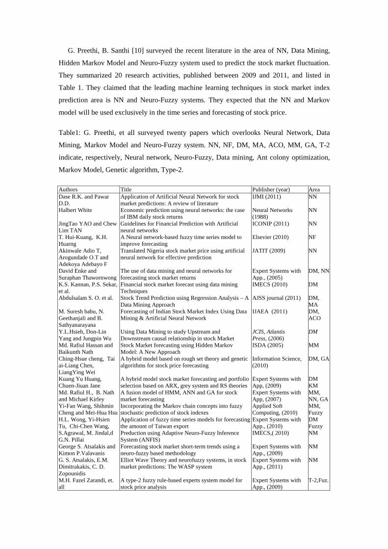
G. Preethi, B. Santhi [10] surveyed the recent literature in the area of NN, Data Mining,

Hidden Markov Model and Neuro-Fuzzy system used to predict the stock market fluctuation.

They summarized 20 research activities, published between 2009 and 2011, and listed in

Table 1. They claimed that the leading machine learning techniques in stock market index

prediction area is NN and Neuro-Fuzzy systems. They expected that the NN and Markov

model will be used exclusively in the time series and forecasting of stock price.

Table1: G. Preethi, et all surveyed twenty papers which overlooks Neural Network, Data

Mining, Markov Model and Neuro-Fuzzy system. NN, NF, DM, MA, ACO, MM, GA, T-2

indicate, respectively, Neural network, Neuro-Fuzzy, Data mining, Ant colony optimization,

Markov Model, Genetic algorithm, Type-2.

Authors Title Publisher (year) Area Dase R.K. and Pawar D.D.

Application of Artificial Neural Network for stock market predictions: A review of literature

IJMI (2011) NN

Halbert White Economic prediction using neural networks: the case of IBM daily stock returns

Neural Networks (1988)

NN

JingTao YAO and Chew Lim TAN

Guidelines for Financial Prediction with Artificial neural networks

ICONIP (2011) NN

T. Hui-Kuang, K.H. Huarng

A Neural network-based fuzzy time series model to improve forecasting

Elsevier (2010) NF

Akinwale Adio T, Arogundade O.T and Adekoya Adebayo F

Translated Nigeria stock market price using artificial neural network for effective prediction

JATIT (2009) NN

David Enke and Suraphan Thawornwong

The use of data mining and neural networks for forecasting stock market returns

Expert Systems with App., (2005)

DM, NN

K.S. Kannan, P.S. Sekar, et al.

Financial stock market forecast using data mining Techniques

IMECS (2010) DM

Abdulsalam S. O. et al. Stock Trend Prediction using Regression Analysis – A Data Mining Approach

AJSS journal (2011) DM, MA

M. Suresh babu, N. Geethanjali and B. Sathyanarayana

Forecasting of Indian Stock Market Index Using Data Mining & Artificial Neural Network

IJAEA (2011) DM, ACO

Y.L.Hsieh, Don-Lin Yang and Jungpin Wu

Using Data Mining to study Upstream and Downstream causal relationship in stock Market

JCIS, Atlantis Press, (2006)

DM

Md. Rafiul Hassan and Baikunth Nath

Stock Market forecasting using Hidden Markov Model: A New Approach

ISDA (2005) MM

Ching-Hsue cheng, Tai ai-Liang Chen, LiangYing Wei

A hybrid model based on rough set theory and genetic algorithms for stock price forecasting

Information Science, (2010)

DM, GA

Kuang Yu Huang, Chuen-Jiuan Jane

A hybrid model stock market forecasting and portfolio selection based on ARX, grey system and RS theories

Expert Systems with App, (2009)

DM KM

Md. Rafiul H., B. Nath and Michael Kirley

A fusion model of HMM, ANN and GA for stock market forecasting

Expert Systems with App, (2007)

MM, NN, GA

Yi-Fan Wang, Shihmin Cheng and Mei-Hua Hsu

Incorporating the Markov chain concepts into fuzzy stochastic prediction of stock indexes

Applied Soft Computing, (2010)

MM, Fuzzy

H.L. Wong, Yi-Hsien Tu, Chi-Chen Wang,

Application of fuzzy time series models for forecasting the amount of Taiwan export

Expert Systems with App., (2010)

DM Fuzzy

S.Agrawal, M. Jindal,d G.N. Pillai

Preduction using Adaptive Neuro-Fuzzy Inference System (ANFIS)

IMECS,( 2010) NM

George S. Atsalakis and Kimon P.Valavanis

Forecasting stock market short-term trends using a neuro-fuzzy based methodology

Expert Systems with App., (2009)

NM

G. S. Atsalakis, E.M. Dimitrakakis, C. D. Zopounidis

Elliot Wave Theory and neurofuzzy systems, in stock market predictions: The WASP system

Expert Systems with App., (2011)

NM

M.H. Fazel Zarandi, et. all

A type-2 fuzzy rule-based experts system model for stock price analysis

Expert Systems with App., (2009)

T-2,Fuz.

Yuehui C. et al. [11] investigated the seemingly chaotic behavior of stock markets using

the flexible neural tree ensemble technique. They examined the 7-year Nasdaq-100 main

index values and 4-year NIFTY index values. Evolutionary algorithm and particle swarm

optimization algorithm were used to optimize the structure and parameter of a flexible neural

tree. They claimed that the most prominent parameters that affect share prices were their

immediate opening and closing values. Chang et al. [12] also applied their methods in the

ensemble neural network. They used AdaBoost algorithm ensembles and two different kinds

of neural net, traditional BPN neural networks and evolving neural networks. Between [12]

and [4], the basic difference is the use of ensemble NN instead of NN. Iffat A. Gheyas et

al.[13] proposed a homogeneous NN ensemble to forecast the time series. They optimized

their method through the generalized regression NN ensemble. Their method was suitable

both for short-term and long-term time series.

3. Methodology The main purpose of this research is to develop a framework that will enable one to

benefit from share market. In order to meet this requirement, a simple and effective method is

proposed. Also, the method is user-friendly and easy to implement. Our method has some

steps, which includes data preprocessing, PLR, input selection, and ensemble neural network.

Stock price prediction has always been a subject of interest for most investors and financial

analysts, but clearly, finding the best time to buy or sell has remained a very difficult task for

investors because there are numerous other factors that may influence the stock price [14, 15].

The entire flowchart is shown in Figure 1. Stock price depends on many factors. For this

reason, the stock price always fluctuates positively or negatively. The prices also vary during

the length of a day. Firstly, the raw data is taken from any stock market, and applied to the

pre-processing steps. Once this is done, the turning point is found. We select some important

technical indexes or some combination of technical indexes using a decision tree algorithm.

The ensemble neural network is used to predict the stock market. If the output of ensemble

neural network does not earn the targetted profit, the decision tree algorithm selects other

indexes. The decision tree algorithm is used as an intelligent formula. Finally, the processes

are stopped.

Fig. 1. Flowchart of entire proposal

3.1 Data Preprocessing

Data preprocessing has been divided into four sub-steps, including data collection, data

rescaling, complexity measure, and data division, which is clearly shown in Figure 2. Each

sub-step is discussed in brief in the following section.

Fig. 2: Data preprocessing steps

3.1.1 Data Collection

The data was collected mainly from three big share markets, namely the Shanghai stock

market (SSM), the Tokyo stock market (TSM), and the NASDAQ100 stock market. Seven

data sets were collected from the Shanghai stock market. The Shanghai stock data covered a

time period from 04/01/2010 to 18/08/2011, and contains approximately 391 days of

Start

Data Pre-processing

PLR

Input Selection

Ensemble NN

Desired Profit

End

Yes

No

Data Collection

Data Rescaling

Complexity Measure

Data Division

transaction data. This data includes up trade, down trade and steady state. From the ten shares,

four are divided into the downturn (Code: 600488, 600054, 600019, 600058), three into

steady trend (Code: 600881, 600228, 600697), and the remaining three are classified as

uptrend (Code: 600051, 600163, 600167) [3]. Ten data sets were collected from the Tokyo

stock market. The Tokyo stock data covered a time period from 10/05/2011 to 15/03/2013,

and approximately 450 days of transaction data. These data hark from five sectors, namely

automotive, communication, electrical machinery, chemicals, and machinery. The selecting

stock indexes are TYO: 7203, TYO: 7267, TYO: 9984, TYO: 9437, TYO: 7751, TYO: 6502,

TYO: 3407, TYO: 4188, TYO: 6305; TYO: 7011, TYO: 6302. We gathered ten stock data

sets arbitrary from NASDAQ100. The data covered a time period from 01/06/2011 to

15/03/2013, covering about 450 days of transaction data. The stock index selecting from the

NASDAQ stock market are AAPL, AMZN, CSCO, COST, ESRX, FB, GILD, GOOG, NXPI,

MSFT, and STX.

3.1.2 Data Rescaling

Stock data have nonlinear characteristic. But, it has some minimum value in a certain

period. We should consider either the time variant data or the frequency data. The time variant

data retains the whole characteristics of data. For this reason, only the upper portion or time

variant data is taken for further analysis. What should be noted is that, if we consider all the

data, the nonlinear behavior effect will be very small in any network. We use the following

equation to normalize all the data in the interval (0,1). 𝑋𝑜𝑜𝑜 ,𝑋𝑚𝑚𝑚 , & 𝑋𝑚𝑚𝑚 are the original,

maximum and minimum values of the raw data respectively, and 𝑋𝑚𝑛𝑛 represents the normalized form

of 𝑋𝑜𝑜𝑜 .

𝑋𝑚𝑛𝑛 =𝑋𝑜𝑜𝑜 − 𝑋𝑚𝑚𝑚

𝑋𝑚𝑚𝑚 − 𝑋𝑚𝑚𝑚

3.1.3 A complexity measure for stock time series

The main purpose behind researching the complexity of the stock market is to contract the

finding into a relation that expresses the proper turning point. Also, the complexity or

simplicity of the time series is gauged by knowing this information. A number of studies have

been conducted to find the complexity for any time series and predict their behavior such as

regular, chaotic, uncertainty, size, etc. The main types of complexity parameters are entropies,

fractal dimensions, Lyapunov exponents [16]. Ahmad kazem et al. [17] used the false nearest

neighbor method to find the minimum sufficient embedding dimension, and the time series

phase was reconstructed to reveal its hitherto unseen dynamics. We chose the Shannon

entropy from these methods to find stock price complexity. Teixeira A. et al. [18] showed that

Shannon entropy effectively measured the expected value. The Shannon entropy is a basic

measure in information theory by calculating uncertainty. The Shannon entropy is calculated

by the following formula

𝐻 = −�𝑝(𝑥𝑚)log𝑏p (𝑥𝑚)𝑚

𝑚=1

Where Shannon entropy is denoted by 𝐻, 𝑥𝑚 is a discrete value from the time series of 𝑋.

The finite number of data is 𝑛 , and 𝑝(𝑥𝑚) shows the probability density function of the

outcome of 𝑥𝑚 . We can say that the complexity of a system is due to the amount of

information. Bigger entropy shows higher complexity for any time series while smaller

entropy shows lower complexity to any time series. It also depends on the size. For this

reason, the average entropy for hundred data is calculated from all data set. According to the

entropy value, the data set is classified as high and low complexity, and this information is

used in the next section. There is a strong relation between entropy and information for any

data set. The Shannon entropy is good for any time series analysis. The average Shannon’s

entropy of 100 data is shown in table 2, where five data sets are chosen arbitrary. Table 2: Average entropy of each 100 data in the data set

Data set Shannon’s Entropy Toyota 6.0824 Mazda 5.0714

Softbank 6.3117 Apple 6.6239 Yahoo 6.2182

3.2 PLR In our proposed PLR measurement, the calculation has been slightly modified from

previous researches. It is very close to the local minimum and local maximum finding method

or local saturation method (LSM). PLR reduces the high frequency and provides a certain

decision for a certain period. Akisato Kimura et al. [19] used PLR to reduce the feature

dimension from long audio signal. PLR is used to find the turning point whether it is the buy,

sell or hold point. Our method also represents buy and sell, respectively, the local minimum

and the local maximum. Many researchers have tended to use many methods, namely Top-

Down, Down-Top and Sliding Window are popular [3].

Let us consider a time series,𝑦 = {𝑦0,𝑦1,𝑦2, … … ,𝑦𝑚}, From this time series, we will find the

approximate piecewise straight lines through the following

𝑦𝑝𝑜𝑝 = {𝐿1(𝑦0,𝑦1, … ,𝑦𝑚𝑛1),𝐿2(𝑦0𝑛2,𝑦1𝑛2, … ,𝑦𝑚𝑛2), …

, 𝐿𝑚(𝑦0𝑛𝑚,𝑦1𝑛𝑚, … ,𝑦𝑚𝑛𝑚)}

Where 𝐿1,𝐿2, … , 𝐿𝑚 represents the line and 𝑚 represents the number of lines, and

𝐿1 = 𝑡1 ∗ 𝑥1 + 𝑐 1, 𝐿2 = 𝑡2 ∗ 𝑥2 + 𝑐 1, 𝐿𝑚 = 𝑡𝑚 ∗ 𝑥𝑚 + 𝑐 1

Here, the slope or gradient 𝑡 and the line 𝑐 intercept (where the line crosses the Y axis)

3.2.1 Finding Turning Point by Local Saturation Methods (LSD)

Local Saturation Method is used to find the proper buying, selling and holding time. LSM

is explained using the following steps. A complete flow chart for LSD is shown in figure 3.

Step1: We have taken the closing stock price in order to find the PLR. The Weighted

Moving Average method is used to smooth the data. The WMA places more importance on

recent stock price moves and less weight on past data. The WMA is calculated by

multiplying each of the previous day’s data by a weight. This is why the WMA responds

rapidly to the stock price movement [20]. The WMA works well to find the proper turning

point. It helps to find big price variation points. The data sets are smoothed by reducing noise.

Step2: We perceive the tangent over the time series. These tangent points act as temporary

turning points. The number of tangent points depends on how much data was taken during the

data smoothing process. If we implement more data smoothing, it will lessen the number of

tangent points or turning points, and vice-versa. We are taking less than ten data smoothing

(such as 3 data points, 5 data points, and 7 data points smoothing).

Step 3: In this step, we identify the immature turning point. If two consecutive data points

show two turning points, we consider these points as immature turning points. Then, the total

immature turning points over the series are reduced. Now, we get mature turning points and

straight lines are drawn from these mature turning points.

The first point and the last point are considered the default turning points. The tangent

points and turning point are calculated from smoothing data, but PLR is drawn from the raw

data. We calculate the slope of each straight line because of the classification class (either buy

or sell or hold). Ethical examples are shown in the fig. 4 where 5 data points’ smoothing are

taken.

0 10 20 30 40 50 60 70 80 90

0.4

0.5

0.6

0.7

0.8

0.9

1

Number of days

No

rma

lize

d P

rice

Step 1

Raw dataSmoothing data

0 10 20 30 40 50 60 70 80 900

0.2

0.4

0.6

0.8

1

Number of Days

Nor

mal

ized

Pric

e

Step 2

Smoothing DataTangent Points

Fig. 3: Graphical representation of LSM steps

The method faces a problem when it comes to finding the appropriate moving average

number. The information or the complexities of time series are used to find the accurate

turning point or proper trade. We know that the complexity depends on the information of any

time series. So, we wanted to establish a relationship between the MA value and the

complexity value. According to the data information, we can deduce two statements:

1. If the data set has high entropy, we will take a high MA number

2. If the data set has low entropy, we will take a low MA number

The main purpose behind measuring the entropy value is to predict the MA number.

Firstly, PLR has been employed to take the MA value through a few fixed numbers. Now,

there is some evidence that the MA value has been taken.

Fig. 4: Complete flow chart for LSM

Our technique is one of the easiest ways to find an accurate PLR. The method we propose

has a few advantages over previous ones. Firstly, there is no need to take threshold values.

Threshold values maintain the full trade such as sell, buy or hold condition. This value is very

sensitive to any kind of time series. We can avoid threshold selection in our method. Secondly,

the optimization of the threshold values is time-consuming when effective learning is

considered. If we avoid this, our learning procedure will be very easy and the learning time

will be reduced. Thirdly, the Shannon entropy is used to find the complexity of the time series

method, considering that the complexity of the moving average number can be automatic.

Fourthly, the WMA is used to implement PLR, which helps to identify proper turning points.

Fifthly, it is very easy to understand, implement and compare with the other methods. A

complete flow chart for PLR is shown in Figure 4.

3.3 Input selection

0 10 20 30 40 50 60 70 80 900.3

0.4

0.5

0.6

0.7

0.8

0.9

1

Number of Days

Nor

mal

ized

Pric

e

PLR

PLRRaw Data

0 10 20 30 40 50 60 70 80 900

0.2

0.4

0.6

0.8

1

Number of Days

Nor

mal

ized

Pric

e

Step 3

Smoothing DataMature Turning Point

Start Stock data

Complexity measure

Local minimum & maximum

measure

MA according complexity

Delete immature tuning point End

3.3.1 Technical indexes Selecting input is another key factor of time series forecasting. A number of factors

influence the stock market. Also, the stock markets have some data regarding their daily stock

price. It is a challenging job to find the accurate technical index combination for forecasting.

The stock market is affected by a number of factors. Many researchers have investigated the

many technical indicators that help to predict the trading signal [21,22,23]. There are some

common factors, such as moving average, transaction volume, bias, related strength. Still, it is

unknown which combination is fit for the stock market predictions.

We propose four new technical indexes which are closely related to the closing transaction

price, and are an effective means to predict the stock price. Firstly, the slope of the time series

can be proposed as a technical index. This technical index is very effective and essential. A

positive slope reflects a positive value, and a negative slope reflects a negative value. Positive

and negative values are very close to buying and selling transaction. The second proposal is a

ten-day MA value of the volume of transaction. The third proposal is a ten-day MA of the

amplitude of the price movement. The second and third proposed indexes are very close to the

closing price transaction. Fig. 5 charts their transaction. The last proposal is the difference

between the normal moving average value and the weighted moving average value. The

difference in value reveals a very significant effect to finding the turning point. If the

difference is high, this effect should be a turning point, and if the difference is small, this

effects no action. Also, if the difference is positive, the turning point should buy point and the

difference is negative, the turning point should sell point.

Fig. 5: Comparison graph for three technical indexes for arbitrary selected stock

3.3.2 Decision Tree

Decision Trees are common algorithms, which are used in various disciplines such as

statistics, machine learning, pattern recognition, and data mining [24]. Decision trees are

0 50 100 150 200 250 300 350 4000

0.1

0.2

0.3

0.4

0.5

0.6

0.7

0.8

0.9

1

Volume (10 data smooting)High-Low (10 data smooting)closing price (3 data smooting)

classifiers on a target attribute in the form of a tree structure. The observations to classify are

composed of attributes and their target value. The nodes of the tree can be decision nodes and

leaf nodes. Decision nodes test a single attribute-value to determine which branch of the sub-

tree applies. Leaf nodes indicate the value of the target attribute [25]. There are many

algorithms for decision tree induction: Hunt Algorithm, CART, ID3, C4.5, SLIQ, and

SPRINT to maintain the most common. The recursive Hunt algorithm, which is one of the

easiest to understand, relies on the test condition applied to a given attribute that discriminates

the observations by their target values.

In most cases, decision tree implementations use pruning. This is a method where a node is

not further split if its impurity measure or the number of observations in the node is below a

certain threshold. The decision tree is a common situation, according to the knowledge–based

recommenders. The existing knowledge domain can be incorporated in the models. The main

advantages of building a classifier using a decision tree are that it is inexpensive to construct,

and it is extremely fast at classifying unknown instances. Another appreciated aspect of the

decision tree is that they can be used to produce a set of rules that are easy to interpret while

maintaining accuracy when compared to other basic classification techniques. The decision

trees are used as an intelligent technical indexes selector. The specific trees are selected for

the specific data sets. The decision tree depends on the value of the profit values. Chang, et al.

[4, 26] has shown a number of technical indices affecting the stock price movement. We use

some input indexes, and in Table 3 presents some input indexes.

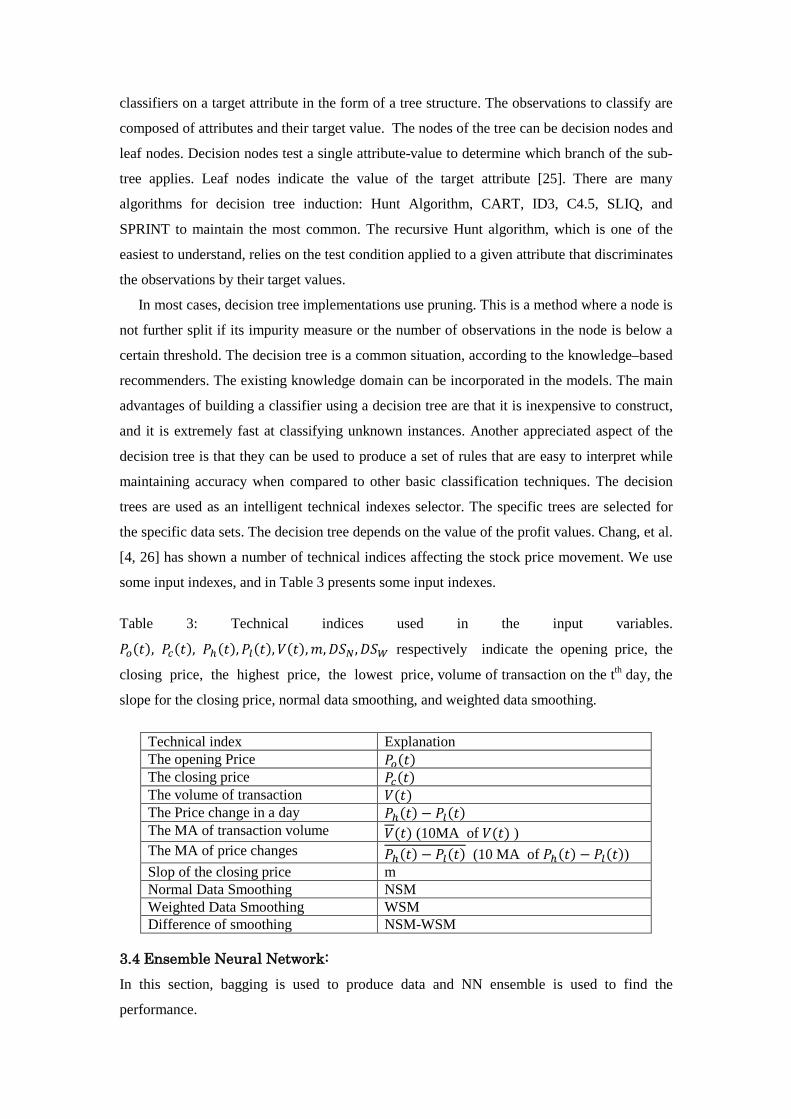
Table 3: Technical indices used in the input variables.

𝑃𝑜(𝑡), 𝑃𝑐(𝑡), 𝑃ℎ(𝑡),𝑃𝑜(𝑡),𝑉(𝑡),𝑚,𝐷𝐷𝑁,𝐷𝐷𝑊 respectively indicate the opening price, the

closing price, the highest price, the lowest price, volume of transaction on the tth day, the

slope for the closing price, normal data smoothing, and weighted data smoothing.

Technical index Explanation The opening Price 𝑃𝑜(𝑡) The closing price 𝑃𝑐(𝑡) The volume of transaction 𝑉(𝑡) The Price change in a day 𝑃ℎ(𝑡) − 𝑃𝑜(𝑡) The MA of transaction volume 𝑉(𝑡) (10MA of 𝑉(𝑡) ) The MA of price changes 𝑃ℎ(𝑡) − 𝑃𝑜(𝑡) (10 MA of 𝑃ℎ(𝑡) − 𝑃𝑜(𝑡)) Slop of the closing price m Normal Data Smoothing NSM Weighted Data Smoothing WSM Difference of smoothing NSM-WSM

3.4 Ensemble Neural Network: In this section, bagging is used to produce data and NN ensemble is used to find the

performance.

3.4.1 Bagging Bagging, a shortened version of Bootstrap Aggregating, is a method that will improve the

unstable prediction or classification task. Leo Breiman [27] introduced the concept of bagging

to construct ensembles. The bootstrap is based on the statistical procedure of sampling with

replacement. New data is created to train each classifier by bootstrapping from the original

data. In the new data, many of the unique patterns may be repeated and many may be left out.

Normally, the data size remains the same. Hence, diversity is obtained with the re-sampling

procedure by the usage of different data subsets. Finally, when an unknown instance is

presented to each individual classifier, a majority or weighted vote is used to infer the class,

and when it is presented to predict, averaging is used to predict values. Table II shows the

Bagging Algorithm steps.

Table 4: Bagging Algorithm

Given training set 𝐷, bagging works in the following

Step 1. Create n bootstrap samples {𝐷0,𝐷1,𝐷2, … … , 𝐷𝑚} of 𝐷 as follows

For each 𝐷𝑚: Randomly drawing |𝐷| examples from 𝐷 with replacement

Step 2. For each 𝑖 = 0,1,2, … ,𝑛 ℎ𝑚 = 𝑙𝑙𝑙𝑙𝑛 (𝐷𝑚)

Step 3. Output 𝐻 =< {ℎ0,ℎ1, … ,ℎ𝑚 } majority vote or averaging

There is a chance that a particular instance will be picked each time the probability is 1/𝑛,

and will not be picked each time probability is 1 − 1/𝑛. Multiply these probabilities together

for a sufficient number of picking opportunities, n, and the result is a formula of

(1 − 1/𝑛)𝑚 ≈ 𝑙−1 = 0.368

On average, about 36.8% of the instances are not present in the bootstrap sample. So, each

bootstrap sample contains only approximately ((1 − 0.368) = 0.632) 63.2% of the instances.

If the learning algorithm is unstable, then bagging almost always improves the performance.

Breiman [28] showed that bagging is effective in “unstable” learning algorithms where small

changes in the training set result in large changes in predictions. Neural networks and decision

trees are examples of unstable learning algorithms. Ten data sets are generated from every

unit in stock market data by Bootstrap aggregation. Bagging reduces the variance, and hence

improves the accuracy.

3.3.2 Neural Network

The ensemble neural network is also known as Committee Methods, Model Combiner.

The ensemble is a learning model where many neural networks are used together to solve a

problem to facilitate better prediction or better classification over a single neural network.

There are two major concerns in this instance: firstly, the individual data sets build techniques

from the unitary patterns; secondly, the question of how output is going to be combined from

every data set. Many methods are available to build individual data sets. Bagging and

boosting are the most popular methods. Bagging generates a diverse ensemble of classifiers

by introducing randomness into the learning algorithm’s input [29].

By applying bagging, we created ten individual sets from every stock data. The complete

ensemble process that was used in our stock market forecasting purpose is shown in Fig. 6.

PLR is created by using a number of straight lines, where each line is represented by an

individual slope. Getting class, we consider a very small threshold value (nearly zero). Three

classes are distinguished by the following ways

If slope value is greater than threshold class 1 [ 𝑚 > 𝑇 Class 1]

If slope value is in between as threshold class 2 [−𝑇 ≤ 𝑚 ≥ 𝑇 Class 2]

Otherwise class 3 [ 𝑚 > −𝑇 Class 3]

[Here,𝑚 and 𝑇 consider as the slope value and the threshold value respectively]

Therefore, majority voting is considered as output class. Also, our network is trained by

supervised NN.

Fig. 6: Ensemble Neural Network

4. Results The most important issue for stock market prediction is the profit or benefit for the

customer or trader. To find the profit, the following formula is used

Profit, 𝑃 = �∑ {(1−𝑚−𝑐).𝑆𝑖−(1+𝑏).𝐵𝑖}(1+𝑏).𝐵𝑖

𝑚𝑚=1 �

Where 𝑙, 𝑏 stands for the transition cost of selling and buying of the 𝑖𝑡ℎ transaction, 𝑐

refers to the tax rate of the 𝑖𝑡ℎ transaction. 𝐷𝑚 ,𝐵𝑚 represents the selling and buying price of the

…..

Stock Data

Bagging Bagging

NN 1

Data 1 Data 2 Data 10 …..

….. NN 2 NN 10

Out 1 Out 2 Out 10

Majority Vote Output

Bagging

𝑖𝑡ℎ transaction, and 𝑛 signifies the number of the transition. Profit is calculated for a single

share. In my methodology, a transaction is complete when the shareholder engages in the

process of minimum buying and selling. Many methods do not make a profit if they do not

consider the tax rate and the transition costs associated with selling and buying.

Two main factors are considered when evaluating our methods, which includes accuracy

and profit. Both are considered in conjunction with customers or shareholders. To evaluate

our method, seven shares are taken from the Shanghai Stock Exchange. Firstly, three shares

are subjected to downtrend, two shares to the steady trend and the last two to uptrend. Table 5,

6, 7 shows the performance results of PLR-ENN. 𝑁𝐵&𝑁𝑆 represents a number of buyers and

sellers, respectively.

During testing, some important considerations are made which are discussed below:

a) Two consecutive buying: It is possible, because investors can buy two times or more. But

at times of sale, investors can sell all their shares at the same time.

b) Two consecutive selling: It is impossible, because investors cannot sell more without

stock. The first sale is considered as a sell point, and the next one is considered as an

unnecessary turning point.

c) First turning point: The first turning point should represent the buy point. If the first

turning point is the sell point, it will be considered an immature turning point. Also, we

are unable to sell shares without buying shares.

d) Last turning point: Last turning point should be the sell point. If instead the last turning

point is the buy point, then the last point of the trade will be considered as a sell point.

e) Two turning points: If the two consecutive turning points represent two transactions days,

it will be considered as an immature turning point. These two turning points should be

reduced by our method. After one sell/buy decision, a minimum of two days are

considered where there is no action.

The most important issue when it comes to predicting the share market is to profit from

the stock market. Our method inclines towards the investor/shareholder. By considering the

above condition, our method works very well. Whenever any investment is made in terms of

money/any decision/any sectors, some time will be consumed in taking further decisions. Our

method has found the more accurate turning points and made a significant amount of profit.

The parameter setting of the ENN, including the number of networks, transfer function,

learning rate, etc. is listed in Table 5. These parameters influence the network performances.

Table 5: Parameters setting for Ensemble Neural network

Number of network

Transfer function

Learning Rate

Iteration Momentum Hidden Layer

Bias Hidden neuron

10 Sigmoid 0.1 1000 1.0 01 1 3-5

The performances of the PLR-ENN are listed in Table 6,7,8 in Shanghai stock market, the

Tokyo stock market, and Nasdaq stock market respectively. We evaluate our method by

calculating the profit, accuracy, the number of buy points (𝑁𝐵), and number of sell point (𝑁𝑆).

From table 6, the Shanghai stock data covered a time period from 04/01/2010 to

18/08/2011 and the last 120 transaction data are used for the test. Among the listed stock from

SSM, the index 600051 shows the highest profit, and that is 108.95% profit. The highest

accuracy as shown in Table 6 is 85.12. There is no negative profit margin.

Table 6: Prediction results of SSM data by PLR-ENN

Indexes 600488 600054 600019 600058 600881 600228 600697 600051 600163 600167 Profit 21.36 14.94 23.34 62.43 33.79 76.31 37.70 108.95 80.89 97.54 Accu. 82.24 74.14 70.85 84.12 78.43 85.12 76.91 84.24 83.12 81.87

𝑁𝐵 6 5 2 8 5 6 6 7 6 6 𝑁𝑆 6 5 2 8 5 6 6 7 6 6

In Table 7, ten data results are presented, which is collected from TSM. TSM is the second

largest stock exchange in the world by aggregate market capitalization of its listed companies.

The collected data from TSM covering from 10/05/2011 to 15/03/2013 time period and the

last 150 transaction data are tested. The highest and lowest profit margins, as shown in the

table, are 113.08% and 38.31% for index 6502 and index 9437, respectively. The height and

lowest accuracy are 88.23% and 68.25%. Our method shows very good outcome.

Table 7: Prediction results of TSM data by PLR-ENN

Indexes 7203 7267 3407 4188 9984 9437 7751 6502 6305 7011 Profit 79.52 85.27 64.49 101.50 56.89 38.31 82.70 113.08 83.32 85.16 Accu. 88.23 75.62 79.16 83.45 68.25 73.14 81.21 87.91 80.98 80.12 𝑁𝐵 6 6 3 6 12 5 11 4 4 3 𝑁𝑆 6 6 3 6 12 6 11 4 4 3

The prediction results of the NASDAQ100 stock market are shown in Table 8. The

historic data cover the financial time-series data from 01/06/2011 to 15/03/2013 and almost

450 transaction data. The last 150 transaction data are taken to evaluate the performances.

NASDAQ100 stocks data also show very good outcome. The percentage of profit cover 22.85

to 77.18 and the percentage of accuracy are 73.15 to 85.21.

Table 8: Prediction results of NASDAQ100 data by PLR-ENN

Indexes AAPL AMZN CSCO COST ESRX GILD GOOG MSFT NXPI STX Profit 28.11 22.85 40.24 32.04 34.82 59.01 36.73 32.52 73.25 77.18 Accu. 77.12 75.13 82.12 80.12 82.12 85.21 75.74 73.64 82.45 73.15 𝑁𝐵 7 7 7 8 7 4 4 12 4 6 𝑁𝑆 7 7 7 8 7 4 4 12 4 6

The graphical representation for nine data set, including closing price and their predicted

trading signal are shown in Figure 7. The data are chosen arbitrarily from three stock markets

(each three). The experiment results show PLR–ENN can mine the hidden knowledge. We

can say that PLR-ENN has a powerful tool for stock price prediction and has excellent

generalization capability.

Fig. 7: Graphical example of predicting turning points.

5. Discussion The comparison results for the Shanghai Stock Market are represented in Table 9. We can

see that PLR-ENN shows the best performance. When it comes to predicting with accuracy,

the PLR-ENN representation is almost double for every case. Our method does not yield any

negative profit compared to the others. PLR-BPN, PLR-WSVM, and PLR-ENN shows that

the minimum profit are -37.05%, -15.32%, and 14.94%, respectively, and the maximum profit

are 22.61%, 50.17%, and 118.95%, respectively. Our method ensures the highest profit and

the highest accuracy. So, PLR-ENN shows a higher generalized ability than PLR–WSVM and

PLR–BPN.

Table 9: The comparison of values vis-à-vis PLR–WSVM, PLR–BPN and PLR-ENN. The

best results are indicated in the bold font.

Indexes Method 𝐴𝐴𝐴 Profit 𝑁𝐵 𝑁𝑆 600488 𝑃𝐿𝑃 − 𝐵𝑁𝑃 33.88 -25.06 3 3

𝑃𝐿𝑃 −𝑊𝐷𝑉𝑊 35.52 -15.32 1 1 𝑃𝐿𝑃 − 𝐸𝑁𝑁 82.24 21.36 6 6

600054 𝑃𝐿𝑃 − 𝐵𝑁𝑃 30.21 -23.87 3 3 𝑃𝐿𝑃 −𝑊𝐷𝑉𝑊 40.63 -2.40 3 3 𝑃𝐿𝑃 − 𝐸𝑁𝑁 74.14 14.94 5 5

6000019 𝑃𝐿𝑃 − 𝐵𝑁𝑃 27.98 -26.46 6 6 𝑃𝐿𝑃 −𝑊𝐷𝑉𝑊 34.72 -13.36 3 3 𝑃𝐿𝑃 − 𝐸𝑁𝑁 70.85 23.34 2 2

600058 𝑃𝐿𝑃 − 𝐵𝑁𝑃 33.51 -37.05 3 3 𝑃𝐿𝑃 −𝑊𝐷𝑉𝑊 44.50 22.16 1 1 𝑃𝐿𝑃 − 𝐸𝑁𝑁 84.12 66.43 8 8

0 20 40 60 80 100 1204.5

5

5.5

6

6.5

7

Days

Code: 600488

Closing PriceBuying PointsSelling Points

0 20 40 60 80 100 1208

9

10

11

12

13

14

Days

Code: 600228

Closing PriceBuying PointsSelling Points

0 20 40 60 80 100 120

10

12

14

16

18

Days

Code: 600051

Closing PriceBuying PointsSelling Points

0 50 100 150

2400

2600

2800

3000

3200

3400

3600

Days

TYO: 7751

Closing PriceBuying PointSelling Point

0 50 100 150300

350

400

450

500

550

Days

TYO: 7011

Closing PriceBuying pointSelling Point

0 50 100 150

400

600

800

000

200

400

600

800

Days

TYO: 7267

Closing PriceBuying pointSelling point

0 50 100 150400

450

500

550

600

650

700

750

Days

AAPL

Closing PriceBuying PointSelling Point

0 50 100 15090

95

100

105

110

Days

COST

Closing PriceBuying PriceSelling Price

0 50 100 15020

25

30

35

Days

NXP

Closing PriceBuying PointSelling pont

600881 𝑃𝐿𝑃 − 𝐵𝑁𝑃 33.15 1.45 7 7 𝑃𝐿𝑃 −𝑊𝐷𝑉𝑊 33.16 4.43 2 2 𝑃𝐿𝑃 − 𝐸𝑁𝑁 39.79 78.43 5 5

600228 𝑃𝐿𝑃 − 𝐵𝑁𝑃 31.02 4.61 8 8 𝑃𝐿𝑃 −𝑊𝐷𝑉𝑊 39.04 33.17 2 2 𝑃𝐿𝑃 − 𝐸𝑁𝑁 85.12 86.31 6 6

600697 𝑃𝐿𝑃 − 𝐵𝑁𝑃 31.02 4.01 7 7 𝑃𝐿𝑃 −𝑊𝐷𝑉𝑊 39.04 33.17 5 5 𝑃𝐿𝑃 − 𝐸𝑁𝑁 76.91 37.70 6 6

600051 𝑃𝐿𝑃 − 𝐵𝑁𝑃 33.16 22.61 2 2 𝑃𝐿𝑃 −𝑊𝐷𝑉𝑊 36.32 50.17 3 3 𝑃𝐿𝑃 − 𝐸𝑁𝑁 84.24 118.95 7 7

600163 𝑃𝐿𝑃 − 𝐵𝑁𝑃 27.84 11.13 6 6 𝑃𝐿𝑃 −𝑊𝐷𝑉𝑊 35.23 9.65 2 2 𝑃𝐿𝑃 − 𝐸𝑁𝑁 83.12 80.89 6 6 600167 𝑃𝐿𝑃 − 𝐵𝑁𝑃 37.82 -2.03 4 4 𝑃𝐿𝑃 −𝑊𝐷𝑉𝑊 44.56 18.64 4 4 𝑃𝐿𝑃 − 𝐸𝑁𝑁 81.87 105.54 6 6

Shannon’s entropy numbers are used as a moving average number. But we cannot say that

this technique is the most effective for every dataset. The stock data set information or

entropy depends on time. It does not show the same entropy value throughout a certain

period. The complexity value depends on the entropy value. It is a difficult task to find the

accurate or exact number of moving averages, but the entropy measurement technique helps

us to find the most accurate moving average number of predictions.

The decision tree algorithm is used as a technical index selector or more effective indexes

for the specific dataset. We know that the decision tree algorithm is a knowledge-based

algorithm. So, there are times when it is difficult to find effective indexes or group of indexes.

It is also possible that the training period suits some indexes, but the testing period witnesses

a decrease in the performance. The decision trees or decision rule algorithms are an effective

method to find a group of dataset for the stock price prediction. The general advantages of

decision trees are that they are well-understood, have been successfully applied in many

domains, and represent a model that can be interpreted relatively easily [30].

The immature data are reduced when PLR is measured. There is little scope to delete an

important turning point. In most cases, manual inspection reveals that our method can find

turning points successfully. Furthermore, the weighted data smoothing, normal data

smoothing, and decision rule will be applied combinely to find this solution.

Undoubtedly, the ensemble neural network has a strong predictive capability. Bagging

creates data diversity, so all necessary information can train the neural network. The network

will be suited to forecasting after the training. If anyone can reprocess their data properly, he

or she can get a significant profit from the stock market. Also, longer time is needed to find

the money that can be invested in order to get the profit. Our method does not work

adequately when it comes to short term prediction.

6. Conclusion

Many researchers have investigated on how to predict the stock market trades properly as

they wanted to present the benefit to the consumer or shareholder. We have charted a

methodology that will foster a simple way for the consumer or shareholder considering which

strategy of buy/sell/hold they can reap the advantage from. Our method shows better results

than PLR-BNP and PLR-WSVM. Firstly, we employed a very simple method to measure

PLR, and this method is also more useful than others. Secondly, our method improves on

previous claims of accuracy. Thirdly, in most cases, our results yielded a higher margin of

profit compared to other methods. Fourthly, we proposed four new technical indexes, which

are very effective for finding turning point or buy/ sell/ hold point.

In the future, the proposed system can be explored by adding other factors or other soft

computing techniques. Areas for further investigations are listed as follows:

1. The data smoothing number will be automatic or will approach a theoretical

background. We will consider more theoretical background to find the appropriate

smoothing number.

2. This paper considered the weighted moving average method of data smoothing.

Furthermore, the general smoothing average, the weighted moving average, and

exponential smoothing average will combine to find more proper turning point or

trade point.

3. Only three stock markets are considered for this research. In the future, we will

consider more well-known stock markets. Anyone can apply our method to any

market and can reap a profit.

4. There are many forecasting models available. We will apply a hybrid intelligent

system for prediction such as Neuro-Fuzzy, NN & Data mining, Fuzzy & Data

Mining etc.

References [1] Tae H. R. “Forecasting the Volatility of Stock Price Index”, Expert Systems with

Applications, 33 (2007), 916-922.

[2] Tsanga, P.M., Kwoka, P., Choya, S.O., Kwanb, R., Nga, S.C., Maka, J., Tsangc, J.,

Koongd K. and Wong, T.L. “Design and Implementation of NN5 for Hong Stock Price

Forecasting”, Engineering Applications of Artificial Intelligence, 20( 2007), 453-461.

[3]Linkai Luo, Xi Chen, “Integrating piecewise linear representation and weighted

support vector machine for stock trading signal prediction”, Journal of Applied Soft

Computing, 13(2013), 806-816.

[4] P.C. Chang, C.Y. Fan, C.H. Liu, “Integrating a piecewise linear representation method and

a neural network model for stock trading points prediction,”IEEE Transactions on Systems,

Man, and Cybernetics, Part C: Applications and Reviews, 39 (2009), 80-92.

[5] P.C. Chang, T.W. Liao, J.J. Lin, C.Y. Fan, “A dynamic threshold decision system for

stock trading signal detection,”Applied Soft Computing, 11(2011), 3998–4010.

[6] Yakup K., M. A. Boyacioglub, Ö. K. Baykanc, “Predicting direction of stock price index

movement using artificial neural networks and support vector machines: The sample of the

Istanbul Stock Exchange,” Expert Systems with Applications, 38 (2011), 5311-5319.

[7] Chih-Fong Tsai, Yuah-Chiao Lin, David C. Yen, Yan-Min Chen, “Predicting stock returns

by classifier ensembles,” Applied soft computing, 11(2011), 2452–2459.

[8] S AbdulsalamSulaimanOlaniyi, Adewole, Kayode S. , Jimoh, R. G, “Stock Trend

Prediction Using Regression Analysis – A Data Mining Approach,”ARPN Journal of Systems

and Software, 1(2011), 154-157.

[9] Gooijer, J. G. D., & Hyndman R. J., “25 years of time series forecasting,” International

Journal of Forecasting, 22 (2006), 443–473.

[10] G. Preethi, B. Santhi, “Stock market forecasting techniques: a survey,”Journal of

Theoretical and Applied Information Technology, 46 (2012), 24-30.

[11] Yuehui Chen, Bo Yang, and Ajith Abraham, “Flexible neural trees ensemble for stock

index modeling,”Neurocomputing, 70 (2006), 697-703.

[12] P. C. Chang, C. H. Liu, C.Y. Fan, J. L. Lin and C. M. Lai, “An Ensemble of Neural

Networks for Stock Trading Decision Making,”ICIC 2, volume 5755(2009) of Lecture Notes

in Computer Science, 1-10.

[13] Gheyas IA & Smith L, “A Novel Neural Network Ensemble Architecture for Time Series

Forecasting,”Neurocomputing, 74 (2011), 3855-3864.

[14] Weckman, G.R., Lakshminarayanan, S., Marvel, J.H., Snow, A., “An integrated stock

market forecasting model using neural networks,” Int. J. Business Forecasting and Marketing

Intelligence, 1 (2008), 30–49.

[15] Chang, P.C. and Liu, C.H., “A TSK type fuzzy rule based system for stock price

prediction,” Expert Systems with Applications, 34 (2008), 135-144.

[16] Christoph Bandt and Bernd Pompe, Permutation Entropy: A Natural Complexity

Measure for Time Series, Physical review letters, 88 (2002), 174102-1-174102-4.

[17] Ahmad Kazem, Ebrahim S., F. Khadeer Hussainb, M. Saberi, O. K. Hussain, “Support

vector regression with chaos-based firefly algorithm for stock market price forecasting,”

Applied soft computing, 13(2013), 947-958.

[18] Teixeira A, Matos A, Souto A, Antunes L. Entropy Measures vs. Kolmogorov

Complexity, Entropy, 13 (2011), 595-611.

[19] A. Kimura, K. Kashino, T. Kurozumi, H. Murase, “A quick search method for

audiosignals based on a piecewise linear representation of feature

trajectories,”IEEETransactions on Audio, Speech and Language Processing, 16 (2008), 396–

407.

[20] http://www.onlinetradingconcepts.com/TechnicalAnalysis/MAWeighted.html

[21] Kyoung-jae Kim, Financial time series forecasting using support vector machines,

Neurocomputing, 55 (2003), 307–319.

[22] Pei-Chann Chang and Chin-Yuan Fan, “A Hybrid System Integrating a Wavelet and

TSK Fuzzy Rules for Stock Price Forecasting,” IEEE SMC Transactions Part C., 38 (2008),

802-815.

[23] Yung-Keun Kwon and Byung-Ro Moon, “A Hybrid Neurogenetic Approach for Stock

Forecasting,”IEEE Transactions on Neural Networks, 18 (2007), 851-864.

[24] L. Rokach and O. Maimon, "Top Down Induction of Decision Trees Classifiers: A

Survey", IEEE SMC Transactions Part C., 35 (2005), 476-487.

[25] Ricci, F.; Rokach, L.; Shapira, B., Kantor, P.B., Recommender Systems Handbook,

Springer, May 2010.

[26] P.C. Chang, Wang, Y.W., Yang, W.N., “An Investigation of the Hybrid Forecasting

Models for Stock Price Variation in Taiwan,” Journal of the Chinese Institute of Industrial

Engineering, 21 (2004), 358–368.

[27] Breiman L., “Bagging predictors,” Machine Learning, 24 (1996), 123–140.

[28] Breiman L., “Stacked regressions,” Machine Learning, 24 (1996), 49-64.

[29] Ian H. Witten, Eibe Frank, and Mark A. Hall, Data Mining: Practical Machine Learning

Tools and Techniques. Morgan Kaufmann, Burlington, MA, third edition, 2011.

[30] Dietmar J. , M. Zanker , A. Felfernig, G. Friedrich , Recommender System: An

Introduction, Cambridge University Press, 2012.

*Corresponding author: Kazuyuki Murase, Ph.D.

Graduate School of Engineering

University of Fukui

3-9-1 Bunkyo, Fukui 910-8507, Japan.

Phone: (+81)(0)776-27-8774, 8735; Fax: (+81)(0)776-27-8420

E-mail: murase@u-fukui.ac.jp

Md. Asaduzzaman is a Ph.D student at the Department of Human and Artificial

Intelligence Systems, University of Fukui, Japan. He has completed his M.Sc. in Electrical

and Electronic Engineering from Khulna University of Engineering and Technology (KUET),

Bangladesh in 2009, and B.Sc. in Electrical and Electronic Engineering from Chittagong

University of Engineering and Technology (CUET), Bangladesh in 2006. His research interest

includes artificial neural networks, Chaos, customer behaviour analysis, and financial time

series.

Md. Shahjahan is working as a Professor at the Department of Electrical and Electronic

Engineering, Khulna University of Engineering and Technology (KUET), Bangladesh. He

received the B.E. degree in Electrical and Electronic Engineering (EEE) from KUET,

Bangladesh, in 1995, the M.E. degree and the Doctoral degree in Information Science

Engineering from University of Fukui, Japan, in 2003 and 2006 respectively. He received the

best student award from IEICE, Hokuriku, Japan, in 2003. His research interest includes

evolutionary robotics, machine learning, feature analysis, human motion analysis, chaotic

neural networks, and pattern recognition.

Fatema Johera Ahmed received her BA (Hons) in English from Lady Shri Ram College

for Women, University of Delhi, India, in 2009, and her MA in English degree in Literature

from BRAC University, Dhaka, Bangladesh, in 2011. Her area of interest includes feminism,

cultural studies, creative writing and editing

Md. Monirul Islam received a B.E. degree in electrical and electronic engineering from

the Bangladesh Institute of Technology (BIT), Khulna, Bangladesh, in 1989, an M.E. degree

in computer science and engineering from Bangladesh University of Engineering and

Technology (BUET), Dhaka, Bangladesh, in 1996, and a Ph.D. degree in evolutionary

robotics from Fukui University, Fukui, Japan, in 2002. From 1989 to 2002, he was a Lecturer

and Assistant Professor with the Department of Electrical and Electronic Engineering, BIT,

Khulna. In 2003, he moved to BUET as an Assistant Professor in the Department of

Computer Science and Engineering, where he is now a Professor. His research interests

include evolutionary robotics, evolutionary computation, neural networks, and pattern

recognition.

Kazuyuki Murase is a Professor in the Department of Human and Artificial Intelligence

Systems, Graduate School of Engineering, University of Fukui, Fukui, Japan, since 1999. He

received an M.E. in Electrical Engineering from Nagoya University in 1978, and a Ph.D. in

Biomedical Engineering from Iowa State University in 1983. He joined as a Research

Associate at the Department of Information Science at Toyohashi University of Technology

in 1984, as an Associate Professor at the Department of Information Science of Fukui

University in 1988, and became a professor in 1992. He is a member of the Institute of

Electronics, Information and Communication Engineers, the Japanese Society for Medical

and Biological Engineering, the Japan Neuroscience Society, and the Society for

Neuroscience. He has served on the Board of Directors of the Japan Neural Network Society,

a Councilor of the Physiological Society of Japan, and a Councilor of the Japanese

Association for the Study of Pain.