Short-Term Inflation Forecasting Models for Nigeria Sani I ...

CBN Journal of Applied Statistics Vol. 4 No.2 (December, 2013) 1

Short-Term Inflation Forecasting Models for Nigeria

1Sani I. Doguwa and Sarah O. Alade

Short-term inflation forecasting is an essential component of the monetary

policy projections at the Central Bank of Nigeria. This paper proposes four

short-term headline inflation forecasting models using the SARIMA and

SARIMAX processes and compares their performance using the pseudo-out-

of-sample forecasting procedure over July 2011 to September 2013.

According to the results the best forecasting performance is demonstrated by

the model based on the all items CPI estimated using the SARIMAX model.

This model is, therefore, recommended for use in short-term forecasting of

headline inflation in Nigeria. The forecasting performance up to eight months

ahead, of the models based on the weighted sum of all items CPI components

is relatively bad. For forecast of food inflation up to ten months ahead

SARIMA is recommended, but for eleven to twelve months ahead the

SARIMAX model performs better. However, the SARIMA model for core

inflation consistently outperforms the SARIMAX model and should therefore

be used to forecast core inflation.

Keywords: Consumer Price Index, SARIMA Process, SARIMAX Process,

Statistical Loss Function, Forecast Evaluation

JEL Classification: C22, E17, E31

1.0 Introduction

The monetary authorities of a large number of countries including Nigeria

have decided that price stability, that is, a low and stable inflation rate, is the

main contribution that monetary policy can give to economic growth.

Accordingly, predicting the future course of inflation in a precise manner is a

crucial objective to maintain this goal, especially in inflation targeting

environment. The Central Bank of Nigeria has the maintenance of monetary

and price stability as one of its mandate. Various monetary policy instruments

are deployed by the Bank to achieve this mandate and the effect of applying

any particular instrument can be felt only after a certain period of time.

Therefore, the Bank is attempting to develop and improve models that will

1 The authors are staff of the Economic Policy Directorate of the Central Bank of Nigeria,

Abuja. The views expressed in this paper are those of the authors and do not necessarily

represent the official views of the Bank. The authors are particularly grateful to O.N. Edem

for the provided research assistance and the anonymous referees whose comments led to the

improvement of the paper.

2 Short-Term Inflation Forecasting Models for Nigeria Doguwa & Alade

provide relatively precise and reliable forecast of the headline, food and core

inflation so that it can react in time and neutralize inflationary or deflationary

pressures that could appear in the future.

Short-term inflation forecasting is an indispensable component of the

monetary policy projection, and therefore, continuous efforts are made to

improve the process at the Central Bank of Nigeria. One way is to improve the

model of short-term forecasting of the Consumer Price Index (CPI) with both

seasonal ARIMA and seasonal ARIMAX processes, where, along with direct

forecasting of the all items CPI, an attempt will also be made to forecast

changes in the 12 international classification of individual consumption by

purpose (COICOP) divisional indices of the CPI. This approach may provide

a more detailed insight into the sources of future inflationary or deflationary

pressures. It will also allow for the determination of whether a forecast of

developments in the CPI obtained by the weighted sum of the index’s

components forecasts is more reliable than a direct forecast.

In this paper, we estimate series of forecasting models that are frequently used

in the short-term forecasting studies of most central banks. While working

with the forecasting models, we employ the all items CPI and its various

components as well as the food and core CPI, as our main variables of

interest. A forecasting model with a good in-sample fit does not necessarily

imply that it will have a good out-of-sample performance. This paper

therefore applies pseudo out-of-sample forecasting technique to evaluate the

forecasting performance of the estimated models.

The objective of this paper is to critically examine the proposed short-term

forecasting models with the view to assessing their pseudo out-of-sample

forecast accuracy using three classical statistical loss functions: - the mean

absolute error (MAE), the root mean squared error (RMSE) and the mean

absolute percent error (MAPE); to determine which of the models are more

precise and reliable over the 12 months forecast horizon. In general, the

smaller the value of the statistical loss function the better the forecast.

For ease of exposition, the paper is structured into seven sections; with section

one as the introduction. Section two reviews both the theoretical and empirical

literature. While section three discusses the methodology, the empirical

analysis and results are presented in section four. Performance evaluations of


the estimated models are contained in section five. Section six provides 12

month forecast of inflation types conditional on the future paths of the

exogenous variables. The final section concludes the paper.

2.0 Review of Theoretical and Empirical Literature

An empirical analysis of causes of inflation in Nigeria by Asogu (1991)

indicated that real output, money supply, domestic food prices, exchange rate

and net exports were the major determinants of inflation in Nigeria. Moser

(1995) and Fakiyesi (1996) studied Nigeria’s headline inflation using both the

long-run and the dynamics error correction model and autoregressive

distributed lag approaches, respectively. Their results confirmed that the basic

findings of Asogu (1991) and agro-climatic conditions were the major factors

influencing inflation in Nigeria. Also, using the framework of error correction

mechanism, Olubusoye and Oyaromade (2008) found that the lagged CPI,

expected inflation, petroleum prices and real exchange rate significantly

propagate the dynamics of inflationary process in Nigeria. More recently,

Adebiyi et al (2010) examined the different types of inflation forecasting

models including ARIMA and showed that ARIMA models were modestly

successful in explaining inflation dynamics in Nigeria.

A lot of empirical research has been conducted in the area of short-term

forecasting using ARIMA models. Akdogan et.al (2012) produced short-term

forecasts for inflation in Turkey, using a large number of econometric models

such as the univariate ARIMA models, decomposition based models, a

Phillips curve motivated time varying parameter model, a suit of VAR and

Bayesian VAR models and dynamic factor models. Their result suggests that

the models which incorporate more economic information outperformed the

random walk model at least up to two quarters ahead.

Mordi et al (2012) developed a short-term inflation forecasting framework to

serve as a tool for analyzing inflation risks in Nigeria. Their framework

follows mostly a structural time series model for each CPI component

constructed at a certain level of disaggregation. Short term forecasts of the all

items CPI is made as a weighted sum of the twelve CPI components forecasts.

Thereafter, the all items CPI and the twelve CPI components are used to

calculate short-term inflation forecasts. The framework is intended to serve as

a tool for analyzing inflation risks with the aid of fan charts and given its


disaggregated nature, appears informative and capable of improving the

credibility of the policy maker.

Pufnik and Kunovac (2006) provided a method of forecasting the Croatia’s

CPI by using univariate seasonal ARIMA models and forecasting future

values of the variables from past behavior of the series. Their paper attempts

to examine whether separate modeling and aggregating of the sub-indices

improves the final forecast of the all items index. The analysis suggests that

given a somewhat longer time horizon (three to twelve months), the most

precise forecasts of all items CPI developments are obtained by first

forecasting the index’s components and then aggregating them to obtain the

all items index.

Alnaa and Ferdinand (2011) used ARIMA approach to estimate inflation in

Ghana using monthly data from June 2000 to December 2010. They found

that ARIMA (6,1,6) is best for forecasting inflation in Ghana. Also, Suleman

and Sarpong (2012) employed an empirical approach to modeling monthly

CPI data in Ghana using the seasonal ARIMA model. Their result showed that

ARIMA (3,1,3) (2,1,1)[12] model was appropriate for modeling Ghana’s

inflation rate. Diagnostic test of the model residuals with the ARCH LM test

and Durbin Watson test indicates the absence of autocorrelations and ARCH

effect in the residuals. The forecast results inferred that Ghana was likely to

experience single digit inflation values in 2012.

Akhter (2013) forecasted the short-term inflation rate of Bangladesh using the

monthly CPI from January 2000 to December 2012. The paper employs the

seasonal ARIMA models proposed by Box et al (1994). Because of the

presence of structural break in the CPI, the study truncates the series and using

data from September 2009 to December 2012 fitted the seasonal ARIMA

(1,1,1) (1,0,1)[12] model. The forecasted result suggests an increasing pattern

and high rates of inflation over the forecasted period of 2013.

Omane-Adjepong et al (2013) examined the most appropriate short-term

forecasting method for Ghana’s inflation. The monthly dataset used was

divided into two sets, with the first set used for modeling and forecasting,

while the second set was used as test. Seasonal ARIMA and Holt-Winters

approaches are used to obtain short-term out of sample forecast. From the

results, they concluded that an out of sample forecast from an estimated


seasonal ARIMA (2,1,2)(0,0,1)[12] model far supersedes any of the Holt-

Winters’ approach with respect to forecast accuracy.

Meyler et al (1998) outlined the practical steps which need to be undertaken

to use ARIMA time series models for forecasting Irish inflation. They

considered two alternative approaches to the issue of identifying ARIMA

models – the Box Jenkins approach and the objective penalty function

methods. The approach they adopted is ‘unashamedly’ one of model mining

with the aim of optimizing forecast performance.

3.0 Methodology

The method of analysis adopted in this study is the Box and Jenkins (1976)

and Box et al (1994) procedure for fitting seasonal ARIMA model. The Box

et al (1994) define the time series {yt}tϵZ as a seasonal ARIMA (p,d,q)

(P,D,Q)[S] process if it satisfies the following equation:

( ) ( )( ) ( ) ( ) ( ) ( )

where L is the standard backward shift operator, φ and Θ are the seasonal

autoregressive (AR) and moving average (MA) polynomials of order P and Q

in variable Ls:

( )

( )

( )

( )

The functions Ø and θ are the standard autoregressive (AR) and moving

average (MA) polynomials of order p and q in variable L:

( )

( )

( )

( )

As an illustration, the SARIMA (1,1,1)(1,0,1)[12] model is a multiplicative

model of the form:

( )( ) ( )(

) ( )

Using the properties of operator L, it follows that equation (6) can be

expressed as:


where Δ is the difference operator. Also d and D are orders of integration and

{ϵt} tϵZ is a Gausian white noise with zero mean and constant variance. Ideally

S equals 12 for monthly data and 4 for quarterly data. The details of ARIMA

modeling procedure are contained in Box and Jenkins (1976), Pankratz (1983)

Box et al (1994) and Asteriou and Hall (2007). For the CPI series under

study, the estimates of the parameters which meet the stationarity and

invertibility conditions are obtained using the Eviews software. The Box et al

(1994) procedure outlined above assumes that (i) the underlying distribution

of the series under study is normal, (ii) the variance is constant and (iii) that

the relationship between the seasonal and non – seasonal components is

multiplicative. When one or all of these conditions are violated the fitted

model may be inadequate for the series under study.

The SARIMAX (or structural SARIMA) process differs from the SARIMA

process ostensibly because it takes cognizance of an exogenous input, which

consists of additional exogenous variables that could explain the behavior of

the dependent variable. Thus, we define the time series {yt}tϵZ as a SARIMAX

(p,d,q) (P,D,Q)[S] process if it satisfies the following equation:

( ) ( )( ) ( ) ( ) ( ) ( ) ( )

The vector Xt constitutes other relevant exogenous variables that are

difference stationary and is the vector of parameter values. As an

illustration, the seasonal ARIMAX (1,1,1) (1,0,1)[12] model with r exogenous

and integrated variables {xit, i=1,2…r} is a multiplicative model of the form:

∑

( )

with the autoregressive term { t} tϵZ satisfying the following condition:

( )( ) ( )(

) ( )


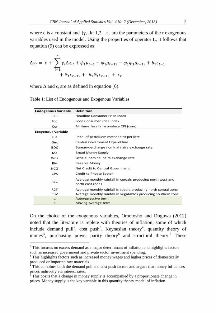
where c is a constant and {γk, k=1,2…r} are the parameters of the r exogenous

variables used in the model. Using the properties of operator L, it follows that

equation (9) can be expressed as:

∑

where Δ and ϵt are as defined in equation (6).

Table 1: List of Endogenous and Exogenous Variables

On the choice of the exogenous variables, Omotosho and Doguwa (2012)

noted that the literature is replete with theories of inflation, some of which

include demand pull2, cost push

3, Keynesian theory

4, quantity theory of

money5, purchasing power parity theory

6 and structural theory.

7 These

2 This focuses on excess demand as a major determinant of inflation and highlights factors

such as increased government and private sector investment spending. 3 This highlights factors such as increased money wages and higher prices of domestically

produced or imported raw materials 4 This combines both the demand pull and cost push factors and argues that money influences

prices indirectly via interest rates. 5 This posits that a change in money supply is accompanied by a proportionate change in

prices. Money supply is the key variable in this quantity theory model of inflation

Endogenous Variable

CPI

Fod

Cor

Exogenous Variable

Fue

Gex

BDC

M2

Wds

RM

NCG

CPS

R1C

R2T

R3V

μ

ɛ Moving Average term

Reserve Money

Net Credit to Central Government

Autoregressive term

Average monthly rainfall in vegatables producing southern zone

Credit to Private Sector

Average monthly rainfall in cereals producing north west and

north east zones

Average monthly rainfall in tubers producing north central zone

Bureau-de-change nominal naira exchange rate

Broad Money Supply

Official nominal naira exchange rate

Definition

Headline Consumer Price Index

Food Consumer Price Index

Price of petroluem motor spirit per litre

Central Government Expenditure

All items less farm produce CPI (core)


theories and earlier empirical studies of inflation in Nigeria by Asogu (1991),

Fakiyesi (1996), Moser (1995) and Olubusoye and Oyaromade (2008) guide

the choice of the exogenous variables used in this paper. Overall, the

exogenous variables considered for inclusion in the short-term forecasting

models are selected based on their theoretical, empirical and situational

relevance. Presented in Table 1 is the list of considered endogenous and

exogenous variables.

The sample for the estimation and forecast evaluation spans the period July

2001 to September 2013 (147 observations) and is divided into two parts. The

first part is the training sample, which includes all monthly data up to June

2011 (120 observations), and the second part is the forecasting sample, which

includes the remaining data from July 2011 to September 2013 (27

observations). The paper uses the training sample to estimate the parameters

of the forecasting models, while the forecasting sample is used for forecast

evaluation.

In the spirit of Meyler et al (1998), Pufnik and Kunovac (2006) and Akdogan

et al (2012), this paper applies a pseudo out-of-sample forecast technique,

which is aimed at replicating the experience that a forecaster faces in a

forecasting practice to evaluate the forecasting performance of the proposed

models. The paper uses the training sample to estimate the parameters of the

forecasting models and as a first step in our forecasting practice obtain one to

twelve months ahead forecasts starting from July 2011 up to June 2012 from

these models. The paper stores these forecasts by putting the first forecast

(July 2011) as first entry in the series 1 step ahead, the second forecast

(August 2011) as the first entry in the series 2 steps ahead and so on to the

twelfth forecast (June 2012) as the first entry in the series 12 steps ahead.

The actual data for July 2011 is added to the training sample after which the

parameters of the models are re-estimated. Using the re-estimated models, we

forecast the values from August 2011 up to July 2012. We then store these

forecasts by putting the first forecast (August 2011) as the second entry in the

series 1 step ahead, the second forecast (September 2011) as the second entry

in the series 2 steps ahead and so on to the twelfth forecast (July 2012) as the

second entry in the series 12 steps ahead.

6 This emphasises the role of exchange rate in the inflationary process, especially in countries

practicing flexible exchange rate regime. 7 This explains that inflation can be caused by structural rigidities in the economy. These

include land tenure, lack of storage facilities, poor harvest, and overdependence on rainfall.


The above exercise is performed repeatedly until we reach the end of the

pseudo out-of-sample period (September 2013). In this way, each of the

forecast exercise yielded 12 series obtained as forecasts from one month

ahead to 12 months ahead, which are then stored accordingly. A series of 16

observations was generated for each time horizon. We tested the quality of the

obtained forecasts using three classical statistical loss functions: Mean

Absolute Error (MAE), Mean Absolute Percent Error (MAPE) and Root Mean

Squared Error (RMSE), defined as follows. Let the series y1t, y2t,..., y16t be the

actual inflation numbers and ŷ1t, ŷ2t, …, ŷ16t be the forecast values for the

forecast horizon t = 1, 2, 3,….12, then:

∑| |

( )

∑

| ( )|

( )

√

{∑( )

} ( )

The two scaled-dependent statistical loss functions: MAEt and RMSEt and the

scaled-independent measure MAPEt for the t forecast horizon (t=1, 2 .., 12)

are used to compare the forecast performances of the estimated short-term

forecasting models.

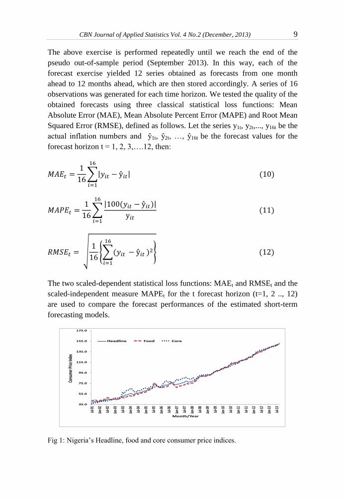
Fig 1: Nigeria’s Headline, food and core consumer price indices.

35.0

55.0

75.0

95.0

115.0

135.0

155.0

175.0

Jul-0

1

Jan-02

Jul-0

2

Jan-03

Jul-0

3

Jan-04

Jul-0

4

Jan-05

Jul-0

5

Jan-06

Jul-0

6

Jan-07

Jul-0

7

Jan-08

Jul-0

8

Jan-09

Jul-0

9

Jan-10

Jul-1

0

Jan-11

Jul-1

1

Jan-12

Jul-1

2

Jan-13

Jul-1

3

Cons

umer

Price

Inde

x

Month/Year

Headline Food Core


4.0 Empirical Analysis and Results

This paper uses actual CPI data from the National Bureau of Statistics (NBS)

covering the period July 2001 to September 2013. Fig 1 shows the trends in

headline; core and food CPI used in the study period for model selection,

parameter estimation and forecast evaluation. A detailed trend analysis of

Nigeria’s inflation and its volatility has been done recently in Omotosho and

Doguwa (2012) and Mordi, et al (2012). The overall basket of products for

calculating the CPI by the NBS is divided into 12 basic product groups in

accordance with COICOP. So the all items CPI is a weighted sum of the 12

basic sub-indices such as food and non-alcoholic beverages; alcoholic

beverages, tobacco and kola; clothing and footwear; amongst others. Thus,

∑

∑

( )

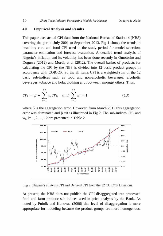
where β is the aggregation error. However, from March 2012 this aggregation

error was eliminated and β =0 as illustrated in Fig 2. The sub-indices CPIi and

wi, i= 1, 2 …, 12 are presented in Table 2.

Fig 2: Nigeria’s all items CPI and Derived CPI from the 12 COICOP Divisions.

At present, the NBS does not publish the CPI disaggregated into processed

food and farm produce sub-indices used in price analysis by the Bank. As

noted by Pufnik and Kunovac (2006) this level of disaggregation is more

appropriate for modeling because the product groups are more homogenous,

-4.00

-3.00

-2.00

-1.00

0.00

1.00

2.00

3.00

4.00

35.00

55.00

75.00

95.00

115.00

135.00

155.00

Jul-0

1

Feb-

02

Sep-

02

Apr-

03

Nov-

03

Jun-

04

Jan-

05

Aug-

05

Mar

-06

Oct

-06

May

-07

Dec-

07

Jul-0

8

Feb-

09

Sep-

09

Apr-

10

Nov-

10

Jun-

11

Jan-

12

Aug-

12

Mar

-13

Aggr

egat

ion

Erro

r

All I

tem

s Co

nsum

er P

rice

Inde

x

Month/Year

CPI wCPI β


while in the 12 COICOP classifications, very different products and services

are placed in the same group. For example, the transport group includes oil

derivatives, whose price changes depend on changes in the price of crude oil

in the international market, and vehicles, whose price changes greatly depend

on the exchange rate and market competition.

Table 2: Headline CPI Sub-Indices and their Weights in the Basket of Products

Checking the order of integration of included variables is crucial in any time

series modeling. The Augmented Dickey Fuller (ADF) and Philips Perron

tests are used to test the stationarity properties of the data. Both tests indicate

that all the variables listed in Tables 1 and 2 are first difference stationary,

except R2T that is level stationary. Box and Jenkins argue that parsimonious

models produce much better forecasts than over parameterized models. They

introduced a three-stage method at selecting a parsimonious seasonal ARIMA

model for the purpose of estimating and forecasting a univariate time series.

The three stages comprise: identification, estimation and diagnostic checking.

The three stage approach was used in this paper. Furthermore, all the

endogenous and exogenous variables used in the paper are in their natural

logarithmic form, except Wds, BDC, NCG, R1C, R2T and R3V.

Before using these parsimonious models for statistical inference, the residuals

ϵt are generally examined for evidence of serial correlation. The Breusch-

Godfrey serial correlation LM test is used to test the null hypothesis of no

serial correlation up to a specific order in the residuals. Also to test the null

hypothesis that there is no autoregressive conditional heteroskedasticity

(ARCH) effect in the residuals, we employ the ARCH LM test. Accepting the

null hypothesis will indicate that there is no ARCH effect in the residuals.

Sub Index Denoted by Weight

CPI1 Fna 0.5180

CPI2 Abt 0.0109

CPI3 Cft Clothing and Footwear 0.0765

CPI4 hwe Housing, Water, Electricity, Gas and other Fuels 0.1673

CPI5 Fhe Furnishing, Household Equipment and Maintenance 0.0503

CPI6 Hea Health 0.0300

CPI7 Trp Transport 0.0651

CPI8 Coc Communication 0.0068

CPI9 Rct Recreation and Culture 0.0069

CPI10 Edu Education 0.0394

CPI11 Rsh Restaurant and Hotels 0.0121

CPI12 Mgs Miscellaneous Goods and Services 0.0166

All Items CPI 1.000

Index Definition

Food and Non-Alcoholic Beverages

Alcoholic beverages, tobacco and kola nuts


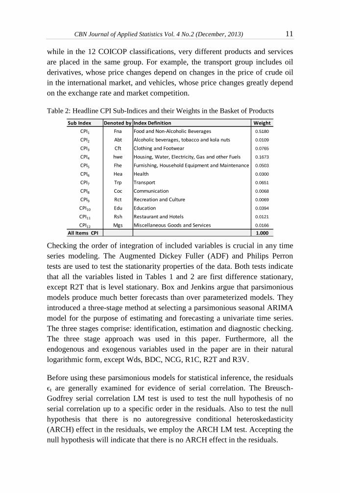
Table 3: Parameter Estimates of the ΔSMhcpit and ΔSXhcpit models

4.1 Parsimonious Headline Inflation Models

In this section we shall provide parsimonious models of the headline CPI

directly using SARIMA and SARIMAX processes. The training sample data

from July 2001 to June 2011 consisting of 120 monthly observations will be

used in the model estimation.

Estimated Models:

Parameter EstimateStandard

ErrorEstimate

Standard

Error

c 0.0089a 0.0004 0.0005a 0.0002

γ1 0.3764a0.0126

γ2 0.5896a0.011

γ3 -0.0034 0.0038

γ4 -0.0044 0.0034

γ5 1.92E-05a6.47E-06

γ6 -8.15E-06c

4.87E-06

γ7 -8.51E-06b4.29E-06

Ø1 0.7528a

0.0744 0.2271a0.0165

Ø2 0.3224a

0.0944

φ1 -0.2856a0.0758 -0.5474a

0.0805

θ1 - 0.6277a

0.0981 -0.9999a0.0262

θ2 -0.0069 0.0941

θ3 -0.3574a0.0892

Θ10.9310a

0.0221 0.8748a0.0234

BG LM Test 1.1385 1.0166

P-Value (0.325) (0.366)

AIC -6.021 -8.906

SC -5.845 -8.569

ARCH LM Test 1.0433 1.0973

P-Value (0.309) (0.297)

Adjusted R - Squared 0.4979 0.9717

a = significant at 1 per cent level

b = significant at 5 per cent level

c = significant at 10 per cent level

All variables are in log form except NCG, R1C, R2T, R3V, Wds, Bdc

ΔSMhcpit ΔSXhcpit


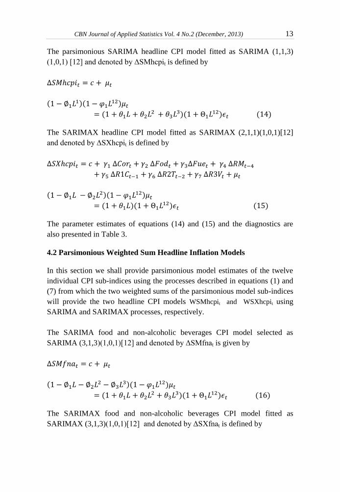
The parsimonious SARIMA headline CPI model fitted as SARIMA (1,1,3)

(1,0,1) [12] and denoted by ΔSMhcpit is defined by

( )(

) (

)(

) ( )

The SARIMAX headline CPI model fitted as SARIMAX (2,1,1)(1,0,1)[12]

and denoted by ΔSXhcpit is defined by

( )(

)

( )( ) ( )

The parameter estimates of equations (14) and (15) and the diagnostics are

also presented in Table 3.

4.2 Parsimonious Weighted Sum Headline Inflation Models

In this section we shall provide parsimonious model estimates of the twelve

individual CPI sub-indices using the processes described in equations (1) and

(7) from which the two weighted sums of the parsimonious model sub-indices

will provide the two headline CPI models WSMhcpit and WSXhcpit using

SARIMA and SARIMAX processes, respectively.

The SARIMA food and non-alcoholic beverages CPI model selected as

SARIMA (3,1,3)(1,0,1)[12] and denoted by ΔSMfnat is given by

(

)( )

(

)( ) ( )

The SARIMAX food and non-alcoholic beverages CPI model fitted as

SARIMAX (3,1,3)(1,0,1)[12] and denoted by ΔSXfnat is defined by


(

)( )

(

)( ) ( )

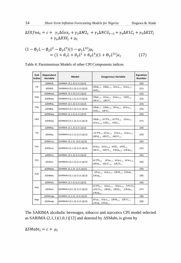
Table 4: Parsimonious Models of other CPI Components indices

The SARIMA alcoholic beverages, tobacco and narcotics CPI model selected

as SARIMA (2,1,1)(1,0,1)[12] and denoted by ΔSMabtt is given by

Sub

Index

Dependent

VariableModel Exogenous Variable

Equation

Number

ΔSMcftt SARIMA (3,1,3) (1,0,1)[12] (20)

ΔSXcftt SARIMAX (3,1,3) (1,0,1)[12] ΔBdct-3, ΔBdct-5, ΔGext-3, ΔGext-7,

ΔM2t-1

(21)

ΔSMhwet SARIMA (4,1,3) (1,0,1)[12] (22)

ΔSXhwet SARIMAX (1,1,1) (1,0,1)[12] ΔBdct-1, ΔFuet-1, ΔGext-3, ΔM2t-2,

ΔR1Ct-1 , ΔR3Vt

(23)

ΔSMfhet SARIMA (3,1,3) (1,0,1)[12] (24)

ΔSXfhet SARIMAX (3,1,3) (1,0,1)[12] ΔBdct-3, ΔBdct-4, ΔFuet-2, ΔGext-2,

ΔM2t-3 , ΔR1Ct

(25)

ΔSMheat SARIMA (2,1,2) (1,0,1)[12] (26)

ΔSXheat SARIMAX (2,1,3) (1,0,1)[12] ΔBdct-2, ΔCPSt-1, ΔCPSt-2, ΔGext-7,

ΔGext-10, ΔM2t-2 , ΔM2t-5

(27)

ΔSMtrpt SARIMA (2,1,2) (1,0,1)[12] (28)

ΔSXtrpt SARIMAX (2,1,1) (1,0,1)[12] ΔCPSt-1, ΔFuet-2, ΔGext-3, ΔGext-9,

ΔRMt-1, ΔR2Tt-2, ΔR3Vt-2

(29)

ΔSMcoct SARIMA (3,1,3) (0,0,1)[12] (30)

ΔSXcoct SARIMAX (1,1,4) (1,0,1)[12] ΔGext, ΔGext-9, ΔM2t, ΔM2t-2,

ΔR1Ct-1, ΔR2Tt-2 , ΔWdst-3, ΔWdst-4

(31)

ΔSMrctt SARIMA (3,1,3) (1,0,1)[12] (32)

ΔSXrctt SARIMAX (3,1,2) (1,0,1)[12] ΔCPSt-4, ΔFuet-1, ΔGext-1, ΔGext-3,

ΔRMt-2, ΔR1Ct-3, ΔR2Tt-1

(33)

ΔSMedut SARIMA (2,1,3) (1,0,1)[12] (34)

ΔSXedut SARIMAX (2,1,3) (1,0,1)[12]

ΔFuet-3, ΔGext-2, ΔRMt-2, ΔWdst,

ΔWdst-1 (35)

ΔSMrsht SARIMA (4,1,4) (1,0,1)[12] (36)

ΔSXrsht SARIMAX (3,1,3) (1,0,1)[12]

ΔCPSt-3, ΔGext-1, ΔGext-8, ΔNCGt,

ΔNCGt-5, ΔRMt-2 ΔRMt-3, ΔWdst-1,

ΔWdst-4

(37)

ΔSMmgst SARIMA (1,1,2) (1,0,1)[12] (38)

ΔSXmgst SARIMAX (3,1,3) (1,0,1)[12] ΔFuet, ΔGext-2, ΔRMt-4, ΔR1Ct-1,

ΔWdst, ΔWdst-1

(39)

Coc

Rct

Edu

Rsh

Mgs

Cft

hwe

Fhe

Hea

Trp


( )(

) ( )( ) ( )

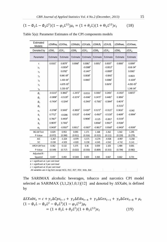
Table 5(a): Parameter Estimates of the CPI components models

The SARIMAX alcoholic beverages, tobacco and narcotics CPI model

selected as SARIMAX (3,1,2)(1,0,1)[12] and denoted by ΔSXabtt is defined

by

(

)( )

( )(

) ( )

Estimated

Models:ΔSMfnat ΔSXfnat ΔSMabtt ΔSXabtt ΔSMcftt ΔSXcftt ΔSMhwet ΔSXhwet

Denoted by ΔSM1 ΔSX1 ΔSM2 ΔSX2 ΔSM3 ΔSX3 ΔSM4 ΔSX4

Parameter Estimate Estimate Estimate Estimate Estimate Estimate Estimate Estimate

c 0.0101a 0.0079a 0.0068a 0.0081a 0.0051a 0.0037c 0.0083a 0.0099a

γ1 -0.0034b -0.0388b -0.0013a -8.6E-04a

γ2 0.0782a -0.1447a -0.0009a 0.0365c

γ3 9.84E-09b 0.0038a -0.0042c0.0023

γ4 1.43E-04a 0.0065a 0.0086a -0.1029a

γ5 -6.87E-05b 0.0676c -4.05E-05b

γ6 5.23E-05b 1.24E-04a

Ø1 -0.5213a 0.3842b -1.2472a0.0153 0.3301a 0.2401c -0.1923c 0.8072a

Ø2 -0.5898a -0.5139a -0.3274a -0.4346a 0.2475a 0.4481a 0.3856a

Ø3 -0.7434a -0.3244c -0.2943a -0.7581a -0.5844a 0.4674a

Ø4 -0.3131a

φ1 -0.3768a 0.5043a -0.3833a 0.4187a 0.5172a -0.3121a 0.3616a-0.042

θ1 0.7712a-0.0286 0.9133a -0.4546a -0.4567a -0.5150a 0.4699a -0.9994a

θ2 0.7667a 0.4459a 0.9696a-0.125 -0.2817 -0.3159a

θ3 0.9870a 0.7302a 0.8566a 0.9027a -0.9184a

Θ1 0.9439a -0.9507a 0.9011a -0.9307a -0.9817a 0.9569a -0.9459a -0.9599a

BG LM Test 0.029 0.953 0.093 1.171 1.168 2.262 1.542 1.295

P-Value (0.972) (0.390) (0.911) (0.316) (0.315) (0.111) (0.220) (0.279)

AIC -5.267 -5.324 -4.979 -5.571 -4.274 -4.928 -4.997 -5.258

SC -5.038 -4.929 -4.828 -5.238 -4.045 -4.542 -4.742 -5.141

ARCH LM Test 0.362 0.132 5.375 0.36 0.059 1.103 1.484 0.001

P-Value (0.549) (0.717) (0.022) (0.550) (0.809) (0.315) (0.704) (0.982)

Adjusted R -

Squared 0.437 0.492 0.5343 0.603 0.365 0.667 0.662 0.731






The selected SARIMA and SARIMAX models for the remaining ten all items

CPI sub-indices are presented in Table 4 as equations (20) to (39).

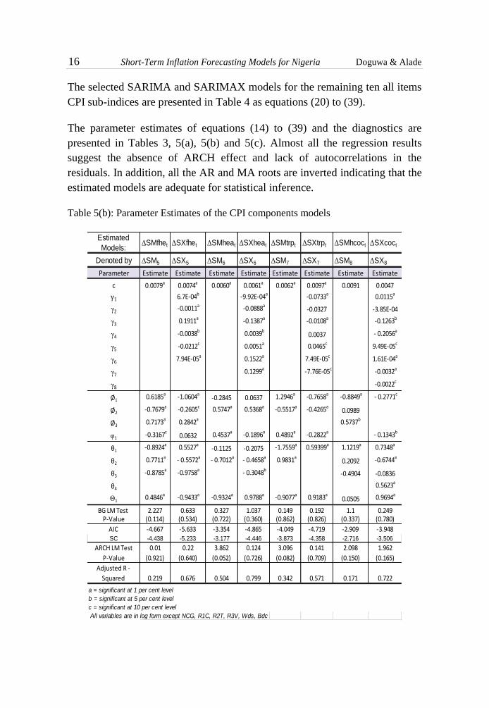
The parameter estimates of equations (14) to (39) and the diagnostics are

presented in Tables 3, 5(a), 5(b) and 5(c). Almost all the regression results

suggest the absence of ARCH effect and lack of autocorrelations in the

residuals. In addition, all the AR and MA roots are inverted indicating that the

estimated models are adequate for statistical inference.

Table 5(b): Parameter Estimates of the CPI components models

Estimated

Models:ΔSMfhet ΔSXfhet ΔSMheat ΔSXheat ΔSMtrpt ΔSXtrpt ΔSMhcoct ΔSXcoct



c 0.0079a 0.0074a 0.0060a 0.0061a 0.0062a 0.0097a 0.0091 0.0047

γ1 6.7E-04b -9.92E-04a -0.0733a 0.0115a

γ2 -0.0011a -0.0888a-0.0327 -3.85E-04

γ3 0.1911a -0.1387a -0.0108a -0.1263b

γ4 -0.0038b 0.0039b0.0037 - 0.2056a

γ5 -0.0212c 0.0051a 0.0465c 9.49E-05c

γ6 7.94E-05a 0.1522a 7.49E-05c 1.61E-04a

γ7 0.1299a -7.76E-05c -0.0032a

γ8 -0.0022c

Ø1 0.6185a -1.0604a-0.2845 0.0637 1.2946a -0.7658a -0.8849a - 0.2771c

Ø2 -0.7679a -0.2605c 0.5747a 0.5368a -0.5517a -0.4265a0.0989

Ø3 0.7173a 0.2842a 0.5737b

φ1 -0.3167c0.0632 0.4537a -0.1896a 0.4892a -0.2822a - 0.1343b

θ1 -0.8924a 0.5527a-0.1125 -0.2075 -1.7559a 0.59399a 1.1219a 0.7348a

θ2 0.7711a - 0.5572a - 0.7012a - 0.4658a 0.9831a0.2092 -0.6744a

θ3 -0.8785a -0.9758a - 0.3048b-0.4904 -0.0836

θ4 0.5623a

Θ1 0.4846a -0.9433a -0.9324a 0.9788a -0.9077a 0.9183a0.0505 0.9694a

BG LM Test 2.227 0.633 0.327 1.037 0.149 0.192 1.1 0.249P-Value (0.114) (0.534) (0.722) (0.360) (0.862) (0.826) (0.337) (0.780)

AIC -4.667 -5.633 -3.354 -4.865 -4.049 -4.719 -2.909 -3.948SC -4.438 -5.233 -3.177 -4.446 -3.873 -4.358 -2.716 -3.506

ARCH LM Test 0.01 0.22 3.862 0.124 3.096 0.141 2.098 1.962

P-Value (0.921) (0.640) (0.052) (0.726) (0.082) (0.709) (0.150) (0.165)

Adjusted R -

Squared 0.219 0.676 0.504 0.799 0.342 0.571 0.171 0.722






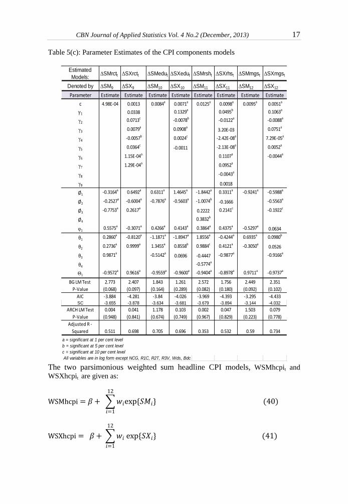
Table 5(c): Parameter Estimates of the CPI components models

The two parsimonious weighted sum headline CPI models, WSMhcpit and

WSXhcpit are given as:

∑ * +

( )

∑ *

+ ( )

Estimated

Models:ΔSMrctt ΔSXrctt ΔSMedut ΔSXedut ΔSMrsht ΔSXrhst ΔSMmgst ΔSXmgst



c 4.98E-04 0.0013 0.0084a 0.0071a 0.0125a 0.0098a 0.0095a 0.0051a

γ1 0.0338 0.1329a 0.0495b 0.1063a

γ2 0.0713c -0.0078b -0.0122a -0.0088a

γ3 0.0079a 0.0908a3.20E-03 0.0751a

γ4 -0.0057b 0.0024c -2.42E-08a 7.29E-05a

γ5 0.0364c-0.0011 -2.13E-08a 0.0052a

γ61.15E-04a 0.1107a -0.0044a

γ71.29E-04a 0.0952a

γ8 -0.0043a

γ9 0.0018

Ø1 -0.3164a 0.6492a 0.6311a 1.4645a -1.8442a 0.3311a -0.9241a -0.5988a

Ø2 -0.2527a -0.6004a -0.7876a -0.5603a -1.0074b

-0.1666 -0.5563a

Ø3 -0.7753a 0.2617a0.2222 0.2141c -0.1922c

Ø40.3832b

φ1 0.5575a -0.3071a 0.4266a 0.4143a 0.3864a 0.4375a -0.5297a 0.0634

θ1 0.2860a -0.8120a -1.1871a -1.8947a 1.8556a -0.4244a 0.6935a 0.0980b

θ2 0.2736a 0.9999a 1.3455a 0.8558b 0.9884c 0.4121a -0.3050a0.0526

θ3 0.9871a -0.5142a0.0696 -0.4447 -0.9877a -0.9166a

θ4 -0.5774a

Θ1 -0.9572a 0.9616a -0.9559a -0.9600a -0.9404a -0.8978a 0.9711a -0.9737a

BG LM Test 2.773 2.407 1.843 1.261 2.572 1.756 2.449 2.351

P-Value (0.068) (0.097) (0.164) (0.289) (0.082) (0.180) (0.092) (0.102)

AIC -3.884 -4.281 -3.84 -4.026 -3.969 -4.393 -3.295 -4.433SC -3.655 -3.878 -3.634 -3.681 -3.679 -3.894 -3.144 -4.032

ARCH LM Test 0.004 0.041 1.178 0.103 0.002 0.047 1.503 0.079

P-Value (0.948) (0.841) (0.674) (0.749) (0.967) (0.829) (0.223) (0.778)

Adjusted R -

Squared 0.511 0.698 0.705 0.696 0.353 0.532 0.59 0.734






where wi are the component weights, ΔSMi and ΔSXi (i=1, 2, …, 12) are

given in Tables 5 (a), (b) and (c) and β is as defined in equation (13).

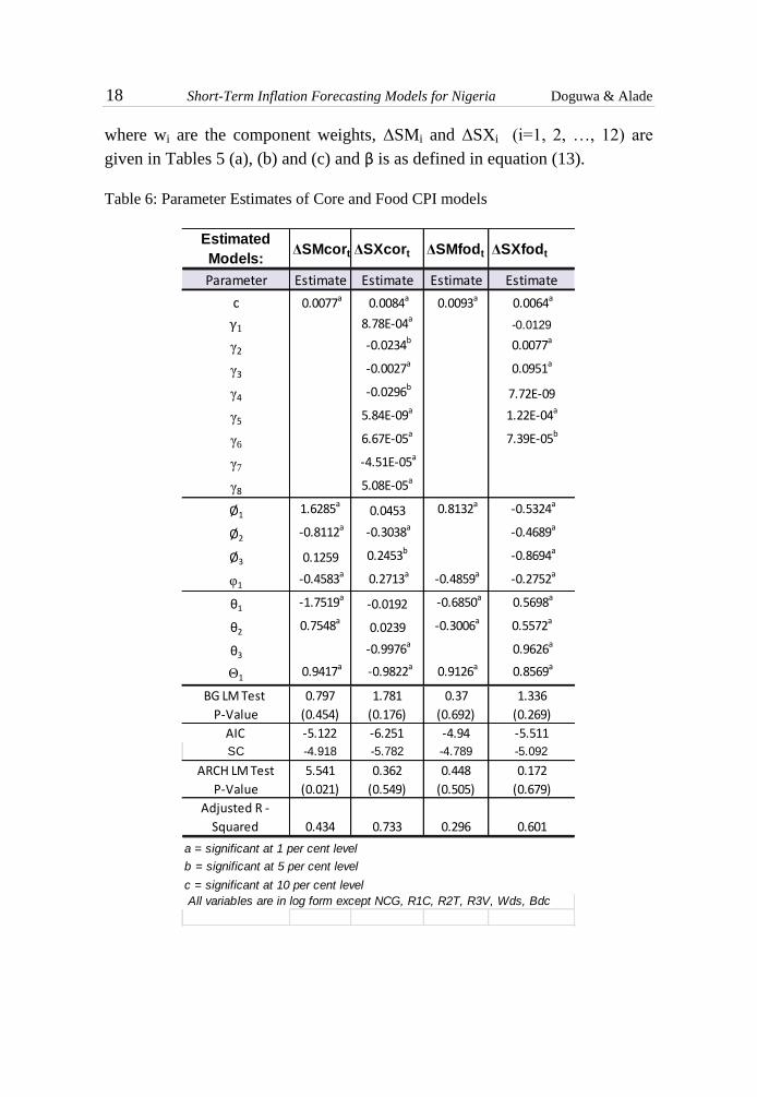
Table 6: Parameter Estimates of Core and Food CPI models

Estimated

Models:ΔSMcort ΔSXcort ΔSMfodt ΔSXfodt

Parameter Estimate Estimate Estimate Estimate

c 0.0077a 0.0084a 0.0093a 0.0064a

γ1 8.78E-04a-0.0129

γ2 -0.0234b 0.0077a

γ3 -0.0027a 0.0951a

γ4 -0.0296b7.72E-09

γ5 5.84E-09a 1.22E-04a

γ66.67E-05a 7.39E-05b

γ7 -4.51E-05a

γ8 5.08E-05a

Ø1 1.6285a0.0453 0.8132a -0.5324a

Ø2 -0.8112a -0.3038a -0.4689a

Ø3 0.1259 0.2453b -0.8694a

φ1 -0.4583a 0.2713a -0.4859a -0.2752a

θ1 -1.7519a-0.0192 -0.6850a 0.5698a

θ2 0.7548a0.0239 -0.3006a 0.5572a

θ3 -0.9976a 0.9626a

Θ1 0.9417a -0.9822a 0.9126a 0.8569a

BG LM Test 0.797 1.781 0.37 1.336

P-Value (0.454) (0.176) (0.692) (0.269)

AIC -5.122 -6.251 -4.94 -5.511

SC -4.918 -5.782 -4.789 -5.092

ARCH LM Test 5.541 0.362 0.448 0.172

P-Value (0.021) (0.549) (0.505) (0.679)

Adjusted R -

Squared 0.434 0.733 0.296 0.601






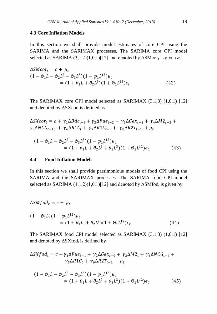
4.3 Core Inflation Models

In this section we shall provide model estimates of core CPI using the

SARIMA and the SARIMAX processes. The SARIMA core CPI model

selected as SARIMA (3,1,2)(1,0,1)[12] and denoted by ΔSMcort is given as

(

)( )

( )(

) ( )

The SARIMAX core CPI model selected as SARIMAX (3,1,3) (1,0,1) [12]

and denoted by ΔSXcort is defined as

(

)( )

(

)( ) ( )

4.4 Food Inflation Models

In this section we shall provide parsimonious models of food CPI using the

SARIMA and the SARIMAX processes. The SARIMA food CPI model

selected as SARIMA (1,1,2)(1,0,1)[12] and denoted by ΔSMfodt is given by

( )( )

( )(

) ( )

The SARIMAX food CPI model selected as SARIMAX (3,1,3) (1,0,1) [12]

and denoted by ΔSXfodt is defined by

(

)( )

(

)( ) ( )


The parameter estimates of equations (42) to (45) and the diagnostics

presented in Table 6 suggest the absence of ARCH effect (except for core

SARIMA) and lack of autocorrelation in the residuals. Also, the assumption

that the AR and MA roots are inverted is satisfied inferring that the fitted

models are adequate for statistical inference.

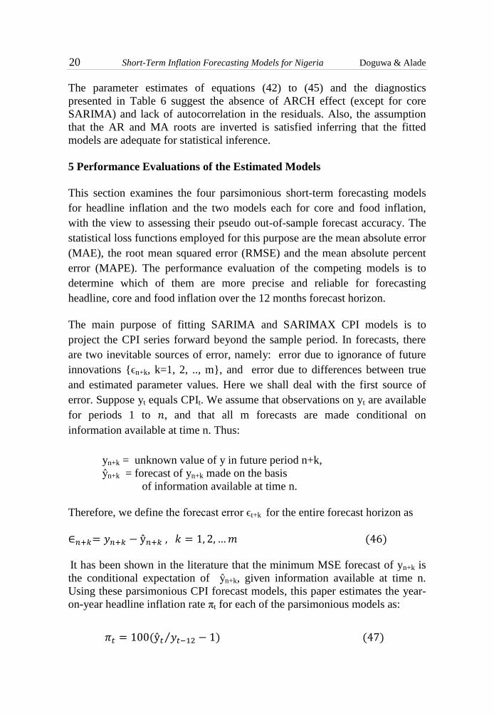
5 Performance Evaluations of the Estimated Models

This section examines the four parsimonious short-term forecasting models

for headline inflation and the two models each for core and food inflation,

with the view to assessing their pseudo out-of-sample forecast accuracy. The

statistical loss functions employed for this purpose are the mean absolute error

(MAE), the root mean squared error (RMSE) and the mean absolute percent

error (MAPE). The performance evaluation of the competing models is to

determine which of them are more precise and reliable for forecasting

headline, core and food inflation over the 12 months forecast horizon.

The main purpose of fitting SARIMA and SARIMAX CPI models is to

project the CPI series forward beyond the sample period. In forecasts, there

are two inevitable sources of error, namely: error due to ignorance of future

innovations {ϵn+k, k=1, 2, .., m}, and error due to differences between true

and estimated parameter values. Here we shall deal with the first source of

error. Suppose yt equals CPIt. We assume that observations on yt are available

for periods 1 to , and that all m forecasts are made conditional on

information available at time n. Thus:

yn+k = unknown value of y in future period n+k,

ŷn+k = forecast of yn+k made on the basis

of information available at time n.

Therefore, we define the forecast error ϵt+k for the entire forecast horizon as

( )

It has been shown in the literature that the minimum MSE forecast of yn+k is

the conditional expectation of ŷn+k, given information available at time n.

Using these parsimonious CPI forecast models, this paper estimates the year-

on-year headline inflation rate πt for each of the parsimonious models as:

( )⁄ ( )


where

ŷt = forecast of CPIt obtained from the

parsimonious CPI model.

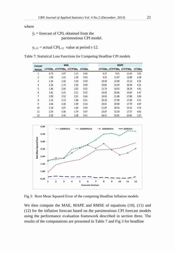
yt-12 = actual CPIt-12 value at period t-12. Table 7: Statistical Loss Functions for Competing Headline CPI models

Fig 3: Root Mean Squared Error of the competing Headline Inflation models

We then compute the MAE, MAPE and RMSE of equations (10), (11) and

(12) for the inflation forecast based on the parsimonious CPI forecast models

using the performance evaluation framework described in section three. The

results of the computations are presented in Table 7 and Fig 3 for headline

ΔSMhlint ΔSMWhlint ΔSXWhlint ΔSXhlint ΔSMhlint ΔSMWhlint ΔSXWhlint ΔSXhlint

1 0.73 1.07 1.31 0.46 6.27 9.31 11.65 3.91

2 1.09 1.41 1.59 0.54 9.25 11.97 13.89 4.58

3 1.24 1.56 1.50 0.50 10.44 13.00 13.12 4.25

4 1.26 1.73 1.92 0.49 10.85 14.29 16.94 4.21

5 1.46 2.05 2.02 0.52 12.74 16.92 18.29 4.41

6 1.81 2.41 2.21 0.52 16.03 20.66 19.65 4.47

7 2.09 2.52 2.01 0.46 19.05 21.80 17.80 3.93

8 2.16 3.13 1.98 0.51 20.18 27.90 17.69 4.51

9 2.06 3.30 1.99 0.53 20.01 29.90 17.79 4.97

10 2.18 3.07 1.60 0.50 21.87 28.34 15.01 4.76

11 2.24 3.36 1.74 0.47 23.07 32.50 17.57 4.62

12 2.50 3.35 2.28 0.51 26.51 32.81 23.65 5.27

MAE MAPEForecast

Horizon

0.50

1.00

1.50

2.00

2.50

3.00

3.50

4.00

1 2 3 4 5 6 7 8 9 10 11 12

Root

Mea

n Sq

uare

d Er

ror

Forecast Horizon

ΔSMhlint ΔSMWhlint ΔSXWhlint ΔSXhlint


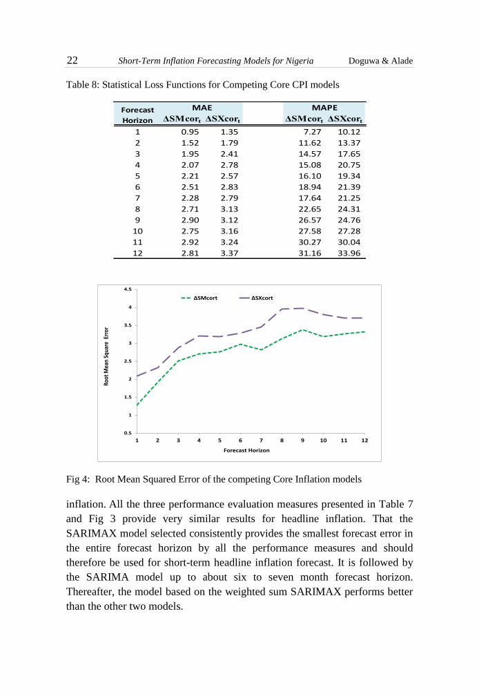
Table 8: Statistical Loss Functions for Competing Core CPI models

Fig 4: Root Mean Squared Error of the competing Core Inflation models

inflation. All the three performance evaluation measures presented in Table 7

and Fig 3 provide very similar results for headline inflation. That the

SARIMAX model selected consistently provides the smallest forecast error in

the entire forecast horizon by all the performance measures and should

therefore be used for short-term headline inflation forecast. It is followed by

the SARIMA model up to about six to seven month forecast horizon.

Thereafter, the model based on the weighted sum SARIMAX performs better

than the other two models.

ΔSMcort ΔSXcort ΔSMcort ΔSXcort

1 0.95 1.35 7.27 10.12

2 1.52 1.79 11.62 13.37

3 1.95 2.41 14.57 17.65

4 2.07 2.78 15.08 20.75

5 2.21 2.57 16.10 19.34

6 2.51 2.83 18.94 21.39

7 2.28 2.79 17.64 21.25

8 2.71 3.13 22.65 24.31

9 2.90 3.12 26.57 24.76

10 2.75 3.16 27.58 27.28

11 2.92 3.24 30.27 30.04

12 2.81 3.37 31.16 33.96

MAE MAPEForecast

Horizon

0.5

1

1.5

2

2.5

3

3.5

4

4.5

1 2 3 4 5 6 7 8 9 10 11 12

Root

Mea

n Sq

uare

Err

or

Forecast Horizon

ΔSMcort ΔSXcort


While the MAE measure presented in Table 8 for core inflation suggests that

the SARIMA model performed better in the entire forecast horizon, the

MAPE measure indicates that for nine and ten months forecast horizon, the

SARIMAX model maybe preferred. However, the RMSE measure given in

Fig 4 indicates that the SARIMA based model has consistently return a lower

error than the SARIMAX and is therefore recommend for use in forecasting

core inflation in the 12 months forecast horizon.

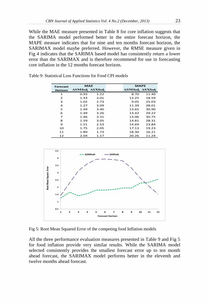
Table 9: Statistical Loss Functions for Food CPI models

Fig 5: Root Mean Squared Error of the competing food Inflation models

All the three performance evaluation measures presented in Table 9 and Fig 5

for food inflation provide very similar results. While the SARIMA model

selected consistently provides the smallest forecast error up to ten month

ahead forecast, the SARIMAX model performs better in the eleventh and

twelve months ahead forecast.

ΔSMfodt ΔSXfodt ΔSMfodt ΔSXfodt

1 0.93 1.22 8.70 11.40

2 1.33 2.01 12.25 18.59

3 1.02 2.73 9.05 25.03

4 1.27 3.09 11.39 28.01

5 1.49 3.40 13.65 30.90

6 1.49 3.26 13.42 29.22

7 1.46 3.31 13.06 30.75

8 1.59 3.05 14.81 28.31

9 1.51 2.53 14.69 23.84

10 1.75 2.05 17.13 19.23

11 1.89 1.73 18.30 16.21

12 2.04 1.17 20.26 11.24

MAE MAPEForecast

Horizon

0.5

1

1.5

2

2.5

3

3.5

4

4.5

1 2 3 4 5 6 7 8 9 10 11 12

Root

Mea

n Sq

uare

Err

or

Forecast Horizon

ΔSMfodt ΔSXfodt


6. Twelve Months Forecast

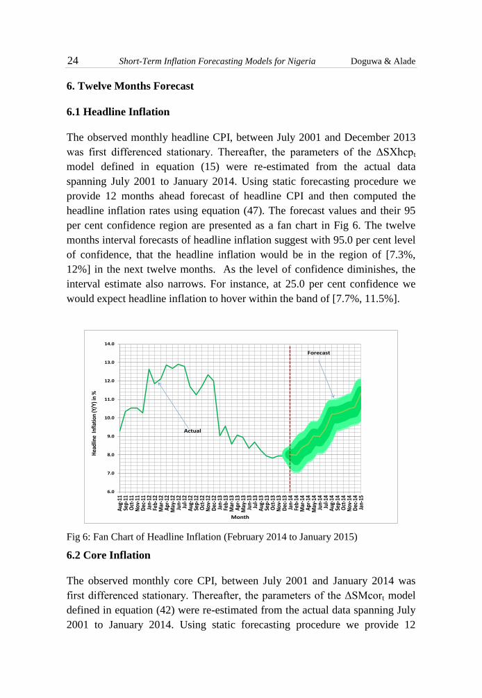
6.1 Headline Inflation

The observed monthly headline CPI, between July 2001 and December 2013

was first differenced stationary. Thereafter, the parameters of the ΔSXhcpt

model defined in equation (15) were re-estimated from the actual data

spanning July 2001 to January 2014. Using static forecasting procedure we

provide 12 months ahead forecast of headline CPI and then computed the

headline inflation rates using equation (47). The forecast values and their 95

per cent confidence region are presented as a fan chart in Fig 6. The twelve

months interval forecasts of headline inflation suggest with 95.0 per cent level

of confidence, that the headline inflation would be in the region of [7.3%,

12%] in the next twelve months. As the level of confidence diminishes, the

interval estimate also narrows. For instance, at 25.0 per cent confidence we

would expect headline inflation to hover within the band of [7.7%, 11.5%].

Fig 6: Fan Chart of Headline Inflation (February 2014 to January 2015)

6.2 Core Inflation

The observed monthly core CPI, between July 2001 and January 2014 was

first differenced stationary. Thereafter, the parameters of the ΔSMcort model

defined in equation (42) were re-estimated from the actual data spanning July

2001 to January 2014. Using static forecasting procedure we provide 12

6.0

7.0

8.0

9.0

10.0

11.0

12.0

13.0

14.0

Aug

-11

Sep-

11O

ct-1

1N

ov-1

1D

ec-1

1Ja

n-12

Feb-

12M

ar-1

2A

pr-1

2M

ay-1

2Ju

n-12

Jul-1

2A

ug-1

2Se

p-12

Oct

-12

Nov

-12

Dec

-12

Jan-

13Fe

b-13

Mar

-13

Apr

-13

May

-13

Jun-

13Ju

l-13

Aug

-13

Sep-

13O

ct-1

3N

ov-1

3D

ec-1

3Ja

n-14

Feb-

14M

ar-1

4A

pr-1

4M

ay-1

4Ju

n-14

Jul-1

4A

ug-1

4Se

p-14

Oct

-14

Nov

-14

Dec

-14

Jan-

15

Hea

dlin

e In

flati

on (Y

/Y) i

n %

Month

Actual

Forecast


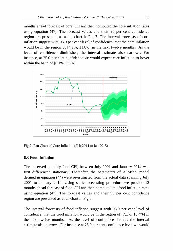
months ahead forecast of core CPI and then computed the core inflation rates

using equation (47). The forecast values and their 95 per cent confidence

region are presented as a fan chart in Fig 7. The interval forecasts of core

inflation suggest with 95.0 per cent level of confidence, that the core inflation

would be in the region of [4.2%, 11.8%] in the next twelve months. As the

level of confidence diminishes, the interval estimate also narrows. For

instance, at 25.0 per cent confidence we would expect core inflation to hover

within the band of [6.1%, 9.8%].

Fig 7: Fan Chart of Core Inflation (Feb 2014 to Jan 2015)

6.3 Food Inflation

The observed monthly food CPI, between July 2001 and January 2014 was

first differenced stationary. Thereafter, the parameters of ΔSMfodt model

defined in equation (44) were re-estimated from the actual data spanning July

2001 to January 2014. Using static forecasting procedure we provide 12

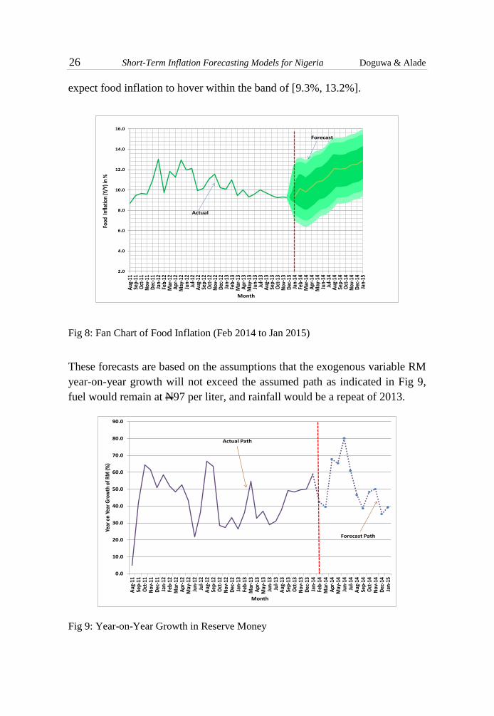
months ahead forecast of food CPI and then computed the food inflation rates

using equation (47). The forecast values and their 95 per cent confidence

region are presented as a fan chart in Fig 8.

The interval forecasts of food inflation suggest with 95.0 per cent level of

confidence, that the food inflation would be in the region of [7.1%, 15.4%] in

the next twelve months. As the level of confidence shrinks, the interval

estimate also narrows. For instance at 25.0 per cent confidence level we would

2.0

4.0

6.0

8.0

10.0

12.0

14.0

16.0

Aug

-11

Sep-

11O

ct-1

1N

ov-1

1D

ec-1

1Ja

n-12

Feb-

12M

ar-1

2A

pr-1

2M

ay-1

2Ju

n-12

Jul-1

2A

ug-1

2Se

p-12

Oct

-12

Nov

-12

Dec

-12

Jan-

13Fe

b-13

Mar

-13

Apr

-13

May

-13

Jun-

13Ju

l-13

Aug

-13

Sep-

13O

ct-1

3N

ov-1

3D

ec-1

3Ja

n-14

Feb-

14M

ar-1

4A

pr-1

4M

ay-1

4Ju

n-14

Jul-1

4A

ug-1

4Se

p-14

Oct

-14

Nov

-14

Dec

-14

Jan-

15

Core

Infla

tion

(Y/Y

) in

%

Month

Actual

Forecast


expect food inflation to hover within the band of [9.3%, 13.2%].

Fig 8: Fan Chart of Food Inflation (Feb 2014 to Jan 2015)

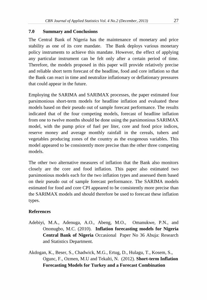
These forecasts are based on the assumptions that the exogenous variable RM

year-on-year growth will not exceed the assumed path as indicated in Fig 9,

fuel would remain at N97 per liter, and rainfall would be a repeat of 2013.

Fig 9: Year-on-Year Growth in Reserve Money

2.0

4.0

6.0

8.0

10.0

12.0

14.0

16.0A

ug-1

1Se

p-11

Oct

-11

Nov

-11

Dec

-11

Jan-

12Fe

b-12

Mar

-12

Apr

-12

May

-12

Jun-

12Ju

l-12

Aug

-12

Sep-

12O

ct-1

2N

ov-1

2D

ec-1

2Ja

n-13

Feb-

13M

ar-1

3A

pr-1

3M

ay-1

3Ju

n-13

Jul-1

3A

ug-1

3Se

p-13

Oct

-13

Nov

-13

Dec

-13

Jan-

14Fe

b-14

Mar

-14

Apr

-14

May

-14

Jun-

14Ju

l-14

Aug

-14

Sep-

14O

ct-1

4N

ov-1

4D

ec-1

4Ja

n-15

Food

Inf

lati

on (Y

/Y) i

n %

Month

Actual

Forecast

0.0

10.0

20.0

30.0

40.0

50.0

60.0

70.0

80.0

90.0

Aug

-11

Sep-

11O

ct-1

1N

ov-1

1D

ec-1

1Ja

n-12

Feb-

12M

ar-1

2A

pr-1

2M

ay-1

2Ju

n-12

Jul-1

2A

ug-1

2Se

p-12

Oct

-12

Nov

-12

Dec

-12

Jan-

13Fe

b-13

Mar

-13

Apr

-13

May

-13

Jun-

13Ju

l-13

Aug

-13

Sep-

13O

ct-1

3N

ov-1

3D

ec-1

3Ja

n-14

Feb-

14M

ar-1

4A

pr-1

4M

ay-1

4Ju

n-14

Jul-1

4A

ug-1

4Se

p-14

Oct

-14

Nov

-14

Dec

-14

Jan-

15

Year

on

Year

Gro

wth

of R

M (%

)

Month

Actual Path

Forecast Path


7.0 Summary and Conclusions

The Central Bank of Nigeria has the maintenance of monetary and price

stability as one of its core mandate. The Bank deploys various monetary

policy instruments to achieve this mandate. However, the effect of applying

any particular instrument can be felt only after a certain period of time.

Therefore, the models proposed in this paper will provide relatively precise

and reliable short term forecast of the headline, food and core inflation so that

the Bank can react in time and neutralize inflationary or deflationary pressures

that could appear in the future.

Employing the SARIMA and SARIMAX processes, the paper estimated four

parsimonious short-term models for headline inflation and evaluated these

models based on their pseudo out of sample forecast performance. The results

indicated that of the four competing models, forecast of headline inflation

from one to twelve months should be done using the parsimonious SARIMAX

model, with the pump price of fuel per liter, core and food price indices,

reserve money and average monthly rainfall in the cereals, tubers and

vegetables producing zones of the country as the exogenous variables. This

model appeared to be consistently more precise than the other three competing

models.

The other two alternative measures of inflation that the Bank also monitors

closely are the core and food inflation. This paper also estimated two

parsimonious models each for the two inflation types and assessed them based

on their pseudo out of sample forecast performance. The SARIMA models

estimated for food and core CPI appeared to be consistently more precise than

the SARIMAX models and should therefore be used to forecast these inflation

types.

References

Adebiyi, M.A., Adenuga, A.O., Abeng, M.O., Omanukwe, P.N., and

Ononugbo, M.C. (2010). Inflation forecasting models for Nigeria

Central Bank of Nigeria Occasional Paper No 36 Abuja: Research

and Statistics Department.

Akdogan, K., Beser, S., Chadwick, M.G., Ertug, D., Hulagu, T., Kosem, S.,

Ogunc, F., Ozmen, M.U and Tekalti, N. (2012). Short-term Inflation

Forecasting Models for Turkey and a Forecast Combination


Analysis, Turkiye Cumhuriyet Merkez Bankasi Working Paper No

12/09.

Akhter, T (2013). Short-term Forecasting of Inflation in Bangladesh with

Seasonal ARIMA Processes Munich Personal RePEc Archive Paper

No 43729 http://mpra.ub.uni-muenchen.de/43729

Alnaa, S.E. and A. Ferdinanad (2011). ARIMA Approach to Predicting

Inflation in Ghana. J. Econ. Int. Finance, Vol 3 no 5, 328-336

Asogu, J.O. (1991). An Econometric Analysis of the Nature and Causes of

Inflation in Nigeria. Central Bank of Nigeria Economic and

Financial Review, 29, 19-30.

Asteriou, D. and Hall, S.G. (2007). Applied Econometrics: A Modern

Approach Using EViews and Microfit. Revised edition, Palgrave

Macmillan

Box, G.E.P. and Jenkins, G.M. (1976). Time Series Analysis: Forecasting

and Control. San Francisco: Holden-Day.

Box, G.E.P., Jenkins G.M and Reinsel, G.C (1994) Time series Analysis;

forecasting and control, Prentice-Hall, New Jersey

Fakiyesi, O.M. (1996). Further Empirical Analysis of Inflation in Nigeria.

Central Bank of Nigeria Economic and Financial Review 34, 489-

499.

Meyler A., Kenny, G., and Quinn, T (1998). Forecasting Irish Inflation

Using ARIMA Models, Technical Paper Series 3/RT/98, Central

Bank and Financial Services Authority of Ireland, 1-48

Mordi, C.N.O., Adebiy, M.A., and Adamgbe, E.T (2012). Short-term

inflation forecasting for monetary policy in Nigeria, Central Bank

of Nigeria Occasional Paper No 42

Moser, G. (1995). The main determinants of inflation in Nigeria. IMF Staff

Papers 42.

http://mpra.ub.uni-muenchen.de/43729


Omane-Adjepong, M., F.T. Oduro., and S.D. Oduro (2013). Determining the

Better Approach for Short-Term Forecasting of Ghana’s Inflation:

Seasonal ARIMA Vs Holt-Winters. International Journal of

Business, Humanities and Technology Vol. 3 No. 1: 69-79

OLubusoye, O.E. and Oyaromade, R (2008). Modeling the Inflation Process

in Nigeria: http://www.aercafrica.org/documents/RP182.pdf

Omotosho, B.S. and S.I. Doguwa (2012). Understanding the Dynamics of

Inflation Volatility in Nigeria: A GARCH Perspective, CBN Journal

of Applied Statistics, Vol.3 No 2: 51-74

Pankratz, A., (1983). Forecasting with Univariate Box-Jenkins Model,

(New York: John Wiley and Sons).

Pufnik, A. and D. Kunovac (2006). Short-Term Forecasting of Inflation in

Croatia with Seasonal ARIMA Processes. Working Paper, W-16,

Croatia National Bank.

Suleman, N. and S. Sarpong (2012). Empirical Approach to Modeling and

Forecasting Inflation in Ghana. Current Research Journal of

Economic Theory Vol. 4, no 3 : 83-87.

http://www.aercafrica.org/documents/RP182.pdf

Short-Term Inflation Forecasting Models for Nigeria Sani I ...

Documents

Transcript of Short-Term Inflation Forecasting Models for Nigeria Sani I ...