Shills and Snipes

Subir Bose, University of Leicester, UK

Arup Daripa, Birkbeck, University of London

Working Paper No. 14/12

September 2014

Shills and Snipes

Subir BoseUniversity of Leicester

sb345@leicester.ac.uk

Arup Daripa

Birkbeck, University of London

a.daripa@bbk.ac.uk

September 2014

Abstract

Online auctions with a fixed end-time often experience a sharp increase in bidding

towards the end despite using a proxy-bidding format. We provide a novel explana-

tion of this phenomenon under private values. We study a correlated private values

environment in which the seller bids in her own auction (shill bidding). Bidders se-

lected randomly from some large set arrive randomly in an auction, then decide when

to bid (possibly multiple times) over a continuous time interval. A submitted bid ar-

rives over a continuous time interval according to some stochastic distribution. The

auction is a continuous-time game where the set of players is not commonly known,

a natural setting for online auctions. Our results are robust with respect to the seller’s

and the bidders’ priors regarding the set of bidders arriving at the auction. We show

that there is a late-bidding equilibrium in which bids are delayed to the latest instance

involving no sacrifice of probability of bid arrival, but shill bids fail to arrive with pos-

itive probability, and in this sense optimal late bidding serves to snipe the shill bids.

We show conditions under which the equilibrium outcome is unique. Further, if these

conditions do not hold, and there are any equilibria with a different outcome, they are

necessarily characterized by early bidding. Any such equilibria are Pareto dominated

for the bidders compared to the late-bidding equilibrium. Finally, our results suggest

that under private values, the case against shill-bidding might be weak.

JEL CLASSIFICATION: D44

KEYWORDS: Online auctions, correlated private values, last-minute bidding, sniping,

shill bidding, random bidder arrival, continuous bid time, continuous bid arrival pro-

cess.

1 Introduction

Online auctions on eBay as well as many other platforms have a pre-announced fixed endtime (“hard end” time), and in many such auctions there is a noticeable spike in biddingactivity right at the end, a phenomenon often called “last minute bidding.” In an Englishauction in which bidding is meant to be done incrementally, such behavior clearly makessense: by bidding just before the auction closes, a bidder might be able to foreclose furtherbids–a practice known as sniping–and win at a low price. To prevent such behavior, eBayallows bidders to use a proxy bidding system.1

Of course, in common value environments, e.g. coin auctions, bidders might have an in-centive to delay their bids even in a proxy bidding auction format in order to optimallyhide the information content of their bids from other bidders.2 However, a large fractionof auctions on online platforms such as eBay fit the private values paradigm well, andexperience significant amount of sniping.3,4 What explains such bidder behavior in a pri-vate values setting? This is the question we address in this paper, and suggest a novelsolution. In contrast with the literature, our analysis establishes the equilibrium bid time

1Under a proxy bidding system, a bidder submits a maximum price, and the proxy bid system then bidsincrementally on behalf of the bidder up to the maximum price. The advantage of the system is that theproxy-bot cannot be sniped: so long as the highest bid of others is lower then the maximum price that abidder has submitted to the proxy bid system, the latter wins.

2See Bajari and Hortacsu (2003), Ockenfels and Roth (2006).3See, for example, Roth and Ockenfels (2002) and Wintr (2008) for evidence of late bidding in eBay

auctions for items such as computers, PC components, laptops, monitors etc. Wintr reports that on eBay,around 50% of laptop auctions and 45% of auctions for monitors receive their last bid in the last 1 minute,while around 25% of laptop auctions and 22% of monitor auctions receive their last bid in the last 10 sec-onds. These items are fairly standardized products and would seem to fit the private values frameworkmuch better than a common values one. While the quality of, say, a laptop may indeed vary affecting in asimilar fashion the payoff of anyone who buys it, the crucial point is that it is unlikely that some bidders arebetter informed about the quality than others. With items such as coins, on the other hand, some biddersmay have greater expertise than others in recognizing the true worth of the items. In such auctions, biddingbehavior of experts may give away valuable information to the non-experts, prompting late bidding by theexperts.

4It is the fixed ending that makes sniping possible. One way to submit a late bid is to use a sniping ser-vice. Several online sites offer this service, and have active user bases. See sites such as auctionsniper.com,gixen.com, ezsniper.com, bidsnapper.com. From site-provided lists of recent auctions won using its service,comments on the discussion forum, or user testimonials it is clear that there is an active market for snipingservices.

1

using a framework in which bid times are chosen in a continuous manner and bid arrivaltimes are continuous but random. Further, we allow for random bidder arrival and, asin the case with real life online auctions, neither the identities nor the actual number ofbuyers is assumed to be common knowledge.

We show that there is an equilibrium with a “late-bidding” outcome that is both natu-ral and intuitive. Moreover, such an outcome is unique under a monotonicity condition(discussed below) on bidder strategies. Further, in the absence of monotonicity, if thereis any equilibrium with a different outcome, it is Pareto dominated for bidders comparedto an equilibrium with late bidding. Importantly, the results are unaffected by either theset of bidders who participate or by the exact nature of the random arrival process. Norare they affected by the exact nature of the priors over these. Therefore the results have a“robustness” with respect to aspects of the environment about which at least the modeler,and also perhaps the seller and the bidders, are unlikely to have precise information.

While we consider private value online auctions, the framework that we develop canbe adapted usefully to other online auction settings, or more generally to settings likebargaining with deadlines and randomly arriving outside options. Let us clarify howthe framework differs from the literature. The literature on sniping in online auctions(considering private and common values and other richer settings) typically assume adiscontinuous timing setting where a certain “last point of time” plays a special role. Allbids arrive with probability 1 before the last point of time, irrespective of how close tothis last point of time they have been made. Bids made at the last point of time fail toarrive with some exogenously given probability. Further, other bidders can respond to abid made before the last point in time with certainty but are completely unable to respondif the bid is placed at the last point. In contrast, in our model, there is a fixed end timefor the auction which is no different from other, regular, times, and the bidders choosehow close to the fixed end time they would like to place their bid. In other words, thearrival probability of bids - as also how much time one leaves for one’s rivals to react toone’s action - is a matter of endogenous choice. The questions addressed in the literaturecould be analyzed in the more natural continuous setting of our framework and whilesome of the results would continue to hold, there are others that depend crucially on adiscontinuity between regular time and the last point of time and would unravel if thisdiscontinuous arrival process of bids is removed. We discuss this further later.

Our analysis starts by considering another phenomenon that occurs in online auctions.

2

Sellers often put in bids assuming different identities and/or get others to bid on theirbehalf. While the practice–known as “shill bidding”–is illegal, and frowned upon by theonline auction community, prevention requires verification, which is obviously problem-atic. Legal or not, shill bidding is reported to be widespread in online auctions.5

The principal characteristic of a shill bid–the one that presumably generates all the pas-sion surrounding the issue–is that the seller submits bids above own value in order toraise the final price. In this sense, of course, any non-trivial reserve price (i.e. any re-serve price that is strictly higher than the seller’s own value) in a standard auction is anopenly-submitted shill bid. We know from Myerson (1981) that the optimal reserve priceis positive even when the seller has no value for the object for sale. However, in a stan-dard private-value auction with a known distribution of values, the optimal reserve priceis also the optimal shill bid. In other words, there is no other higher bid that the seller cansubmit (openly or surreptitiously) that would improve revenue.6

In our model, a seller uses an online auction site (like eBay) to try to sell an item. Theauction format used is proxy bidding. The important point of departure is that the sellerfaces some uncertainty about the distribution from which bidder valuations are drawn.In such a setup, bids convey useful information to the seller and–since it is not typicallypossible to openly adjust the reserve price mid-auction–allows scope for profitable shillbidding.

We show that late bidding by bidders is directly related to shill bidding by the seller. Thebidders bid late not because they want to snipe the bids of other bidders but becausethey want to snipe the shill bids. The continuous choice gives rise to interesting resultson bid-timing and efficiency. To clarify, consider the model we analyze. We assume thatthe auction takes place over a time interval stretching from −T to 1. The interval [−T, 0)is the “early” period and [0, 1] is the “last minute” (with evolving technology this is inpractice a short interval of time, perhaps a few seconds rather than an actual minute).A random selection (from some large set) of bidders enter randomly over [−T, 0], and

5See, for example, the The Sunday Times (2007) report on shill bidding on eBay. See also the BBCNewsbeat report Whitworth (2010). In Walton (2006) the author describes how he and his colleagues placeda large number of shill bids on their eBay auctions.

6There might be scenarios – for example if cancelling bids is not costly – where the seller would havean incentive to shill bid even when the distribution is known. While this is not the focus here, it is worthpointing out that the bid-time choice problem of bidders in such scenarios is likely to be similar to that inour model. Footnote 23 comments further on this issue.

3

can submit proxy bids at any time after they enter. Bidders can submit one or more bidsleading up to time 0, and also choose to make a bid inside the last minute (at some pointt ∈ (0, 1)). The arrival time of a bid made at time t is uniformly distributed on [t, t + 1] solong as t 6 0 (so that t + 1 is within end time 1). In other words, early bids made at somet 6 0 arrive eventually with certainty. The last point of time at which this property holdsis time 0. This is the cusp of the last minute. A bid made after time 0 is made at sometime t “inside” the last minute (i.e. at a time t ∈ (0, 1)). Any such bid fails to arrive withprobability t. Bidders could bid at time 0, or sacrifice some arrival probability by pushingtheir bid times to later than 0. These strategies have different implications for revenueand efficiency. We are therefore interested in determining the precise time of bidding.7

The seller chooses an initial reserve price; this is part of the description of the auction.The seller’s strategy consists of submitting shill bids at a finite number of time points.

We show that in any equilibrium, so as to reduce the chances of the seller submitting shillbids successfully, the bidders optimally bid at the very last possible time such that theirbids reach with probability 1. As noted above, in our model this is time 0. Indeed, bid-ding exactly at time 0 is an equilibrium outcome, one that is unique under a monotonicitycondition. Therefore, whenever the auction results in a sale, there is no loss of efficiency.Further, we show that as a result of the bid-time selection by bidders, all shill bids nec-essarily arrive with probability strictly less than 1. Thus the shill bidder is sniped in thesense that there is a positive probability that some or all shill bids do not arrive.

As mentioned earlier, shill bidding is generally considered harmful to bidders’ interests.However, it follows from our results that a clear conclusion cannot be drawn. As al-ready noted, all genuine bids eventually arrive resulting in the sale being efficient whenit happens (efficiency “at the top”). Second, the fact that the seller can increase (prob-abilistically) the reserve price while the auction is ongoing means that the seller mightchoose a lower initial reserve price compared to the case where shill bids are ruled out.This, combined with the fact that some or all shill bids may fail to arrive implies that insome cases the auction with shills realizes trading gains that would be lost in the stan-dard case without shill bids. Thus the auction with shills may be more efficient “at thebottom.”

7Of course, if bidders do not arrive by time 0, they would necessarily bid after time 0. Since our focus ison studying the choice to bid early or late rather than forced late bidding from late arrival, we assume thatall bidders arrive before time 0.

4

Let us now discuss the specific results of our paper. We first show that the seller’s equi-librium strategy involves submitting shill bids only at times when the auction registerssome activity (the reserve price is met or auction price jumps up). To see why this mat-ters, consider the following example of a “threat” strategy by the seller to induce earlybidding by the bidders: the seller submits a “high” shill bid if there has been no activitytill some time t < 0. If the bidders believe this threat then that might induce them to bidearly, allowing the seller to shill bid more successfully. Our result shows that such threatsare not credible. In addition to being of some independent interest, this result plays animportant role in the analysis that follows.

Next, we show that it is suboptimal for the bidders to only bid at a time t > 0 (i.e. onlybid “inside” the last minute). This establishes the crucial result that it is not worthwhileto sacrifice probability-of-bid-arrival in order to snipe shill bids.

Given these results characterizing equilibria, the natural next step is to establish that anequilibrium does exist. We show that there is indeed an equilibrium in simple strategies:submit a truthful bid at time t = 0 irrespective of history up to time 0, and remain inactivethereafter. We also define a monotonicity condition under which bidding at time 0 byall bidders (of types above the initial reserve price) is the unique equilibrium outcome. Ifthere is any equilibrium with early bidding (bidding at some time t < 0), it must thereforeinvolve non-monotonic strategies. The final result shows that from the viewpoint of thebidders, any such equilibrium is Pareto dominated by the one involving bidding at time0.

Since the property of monotonicity of strategies plays a crucial role in some of our results,we now describe it and explain the intuition behind the role it plays.

Suppose strategies have the following simple structure: at any time t, there is a triggerprice pi

t for bidder i, who bids at t if and only if the auction price at t equals or exceedspi

t. We call such strategies “monotonic.” Consider a simple setting with two bidders. Let“bidding early” denote bidding at any time before 0. If bidder 2 follows a monotonicstrategy, bidder 1 cannot be induced to bid early. To see why, note that bidding earlyimplies 1’s bid would arrive early and trigger a shill bid early with positive probability.Also, bidding early implies 2 might bid early (if the auction price reaches p2

t at an earlyt), which in turn might again trigger a shill bid early. Since delaying bidding till time 0involves no loss of bid-arrival probability, but delays triggering shill bids, early biddingby bidder 1 is suboptimal.

5

Can bidders be induced to bid early in an equilibrium? This can happen only if theexpected payoff from deviating (and not bidding early) is sufficiently bad. But how canthat happen? We have argued that it is not possible for the seller to induce early biddingin a credible way. Hence the only way for a bidder (1 say) to bid early in equilibrium isfor bidder 2 to have a strategy in which 2 bids at some time t < 0 if the auction priceis lower than some threshold level but not bid if it is higher. The first part acts as thepunishment against deviation. A sufficiently harmful punishment would induce bidder1 to bid early to raise the probability that the auction price crosses the threshold at time t.Note however, that this (somewhat strange) strategy of player 2 violates monotonicity.8

Since it is suboptimal for bidders to delay bidding beyond time 0 and since under mono-tonicity they do not bid before time 0, it follows that the unique outcome is to bid attime 0. Further, the strategies we propose to show existence are monotonic by construc-tion. Therefore any deviation by a bidder is contemplated in a setting where others adoptmonotonic strategies. It follows that the logic that guarantees uniqueness also provesexistence.

To see how our results differ from the literature, it helps to compare our setting to thatof Ockenfels and Roth (2006) who also provide a rationale for last minute bidding underprivate values. They assume that there exists a “last point” in time (let us call it tL) withthe following property: a bid made at the point tL reaches with probability 0 < p < 1;further, no one can react to such a bid if it reaches. On the other hand, a bid made at timetL − ε for any ε > 0, reaches with probability 1 and the other bidder has time to reactand submit a counter bid which also reaches with probability 1. Given this setup, theyshow that there is a “collusive” equilibrium in which the bidders bid at time tL becauseby doing so each takes a chance that his own bid will go through while the other bidder’sbid will not - allowing the former to win and pay a low price. If anyone deviates and bidsbefore tL, the other retaliates and bids before tL also, and a standard outcome follows.So long as the collusive price is low enough deviations are not profitable. Note however,that if we drop the discontinuity in bid arrival and make the arrival probability of bids acontinuous function of time (a bid made at t < tL reaches with a probability that goes tozero as t→ tL), then starting from the situation where bidders are supposed to be biddingat time tL, each bidder will have an incentive to bid “a little early,” which then unravels

8In other words, any early bidding equilibrium necessarily involves threats to each bidder from otherssaying in effect “bid early or face a higher chance that we will bid earlier than otherwise and facilitate shillbids.”

6

the sniping equilibrium.

Turning to a different feature of the auctions we consider, note that a “hard” end time iscrucial here as it allows bidders to snipe the shill bidder by delaying bids. Alternatively,an auction could have a “soft” ending so that if a bid arrives in the last 5 minutes (say),the end time is automatically extended until there is no bidding activity for 5 continuousminutes - a format used by uBid.com. A soft ending precludes sniping. As Roth andOckenfels (2002) report, the contrast between the two formats gives rise to interestingdifferences in bidding data across auctions. Auctions on eBay, which uses a hard end time,have substantially greater late bidding compared to Amazon auctions (these auctions,now defunct, used a soft ending). Since the purpose of late bidding in our model isto snipe the shill bid, and since this is not possible under a soft ending, our results areconsistent with this finding.9

Relating to the Literature

In our paper, bidders want to delay bids optimally to hide information from the seller.Other papers have considered reasons for bidders to delay bids to hide information fromother bidders. Bajari and Hortacsu (2003) consider a common values setting and assume a(discontinuous) timing structure that implies that an eBay auction is a two stage auction:up to time tL − ε it is an open ascending auction, and for the rest of the time it is a sealedbid auction (i.e. in this stage all bids arrive, but no one can respond to any one else’s bid).Under this structure, they show that all bidders bidding only at the second stage is anequilibrium. Ockenfels and Roth (2006) study a second model of last minute bidding setin a common values environment with two bidders: an expert and a non-expert. Only theexpert knows whether an item is genuine or fake. However the non-expert has a highervalue for a genuine item compared to the expert. The expert does not bid if the item isfake. If the item is genuine, it is then clear that the expert might not want to bid earlyas such bids might reveal to the non-expert that the item is genuine. Assuming the sametiming structure as in their “collusion” theory discussed above, they show that if the priorprobability that the object is fake is high enough, there is an equilibrium in which only the

9In our formal model, all buyers arrive before time t = 0 to avoid trivial last minute bidding. If buyerscan arrive after time 0, there would be some late bidding even in soft end proxy auctions. Holding con-stant buyer arrival rate, one would nevertheless expect more late bidding in hard end rather than soft endauctions which is what the data seems to suggest.

7

expert bids, and bids only at a “last point of time” time tL, thus not giving the non-expertthe chance to react to this information.

Our approach differs from these ideas in that, first, we have a standard private valuessetting in which (ex ante) symmetric bidders know their own valuations and have no in-centive to hide information from other bidders. The reason for late bidding is the desireto reduce the probability that shill bids arrive successfully. Another difference arises be-cause we allow bid times to be chosen continuously. This implies a further connection tothe literature. We could ask how the results in the literature would be modified in ourcontinuous timing framework.

As noted above, the “collusive” equilibrium of Ockenfels and Roth (2006) cannot arise ina framework of continuous bid and arrival times. But other types of equilibria discussedabove–late bidding in a common values framework to discourage aggressive bidding,or an expert bidding late to hide information–could also arise using our continuous-bid-and-arrival-time framework. An interesting question then is to determine the optimal bidtime in these cases.10

Finally, consider the question of shill bidding. Engelberg and Williams (2009) analyzean incremental shill-bidding strategy to discover the high value when bidders, presum-ably due to behavioral biases, bid in predictable units. Here too late bidding would bebeneficial in reducing the scope for successful shill bidding, but obviously such calcula-tions need not apply when behavioral biases or naive decision-making dictate bid-timeselection. In such contexts, our work can be seen as a benchmark model with rational bid-ders, and explaining any observed departures from our conclusions would then requireincorporating more complex environments or behavioral biases.

Chakraborty and Kosmopoulou (2004), Lamy (2009) examine shill bidding in environ-ments with common values or interdependent values, and show that the presence of shillbidding can reduce the information content of the observed auction prices, and reducethe seller’s revenue. Lamy shows how a “shill bidding effect” arises with interdepen-dent values that goes against the usual linkage principle, and therefore favors first priceauctions (immune to shill bids) against second price auctions in revenue ranking. How-ever, unless the seller can credibly commit to abstain from shill bidding, such bids arise

10Rasmusen (2006) models a private values setting in which a high value bidder hides information froma bidder who does not know own value by bidding at a discontinuous last minute. This, too, could beanalyzed using our continuous approach.

8

in equilibrium.

The rest of the paper is organized as follows. The next section presents the model. Sec-tion 3 presents characterization results under monotonicity. Section 4 then proves ourmain results on equilibrium bid-timing under shill bidding. Finally, section 5 concludes.Proofs not in the body of the paper are collected in the appendix.

2 The Model

A seller is interested in selling a single unit of an indivisible object and uses an onlineauction site to try to sell the item. The seller’s own value for the object is zero. Theauction format is proxy bidding with a hard (i.e. fixed) end time. This is a second-priceauction. The seller can post a reserve price at the beginning and also submit shill bidsduring the auction.

Bidders are drawn randomly from some large set N of potential bidders. Bidder arrivalin the auction is allowed to be random. The seller as well as each bidder therefore faces arandom subset of other bidders. The arrival process is independent of the distribution ofvaluations or actual bidder valuations.

While most of standard auction theory assumes the number of bidders to be commonknowledge, it is difficult to justify this assumption for online auctions. In our model thearrival of bidders to the auction is stochastic and private information and consequentlyneither the seller nor the bidders observe the actual number of bidders. While our modelinvolves standard Bayesian rational agents who therefore have priors over different sub-sets of arriving bidders, the equilibrium outcome we are interested in holds irrespectiveof which subset arrives. Thus the prior belief plays no role in our proofs implying thatthe exact nature of the prior belief is unimportant. Therefore our results have a certainrobustness property not often found in (perfect) Bayesian Nash equilibria of many otherauction models.

9

Bidder valuation We analyze shill bidding under a correlated private values setting.Let F denote a set of distributions F1, . . . , FH, where each distribution has support [v, v],where 0 6 v < v < ∞.11 Nature chooses a distribution Fk from the set F and the bidders’values are determined according to independent draws from the distribution Fk. Eachbidder privately observes its own value. Neither the bidders nor the seller observes Fk

but has some prior belief over F .12 We assume that the distributions are ordered in termsof likelihood ratio property. In other words, a higher value of v is more likely to havebeen generated from a distribution Fk′′ than the distribution Fk′ for k′′ > k′. Since dom-inance in terms of likelihood ratio implies dominance in terms of hazard rates, this alsoimplies that the optimal reserve price will be higher for distribution Fk′′ than for Fk′ . Thisis important in providing a reason for shill bidding. If - as in second price auctions - bidsreflect true values, increase in current price (current second highest bid) in the auctionresults in updated posterior beliefs inducing the seller to either maintain status quo or,with positive probability, to want to raise the reserve price.

11We use the word “support” a bit loosely. We allow for intervals [vk, vk] for k ∈ {1, 2, · · · , H} to bedifferent, and then define v = min vk and v = max vk, the union of the supports of the distribution. Howeverwe continue to call [v, v] as the support and this should cause no confusion.

12We need to emphasize that we assume that bidders do not know the distribution only because wethink it is more realistic; however, none of our results would be affected if we had assumed that bidders doknow the distribution. Bidder valuations in our model is private and correlated; the alternative assumptionwould have made them, in addition, conditionally independent. What is crucial is that the seller does notknow the distribution.

10

-

0−T 1

tt tt + 1

Early� - LastMinute

� -

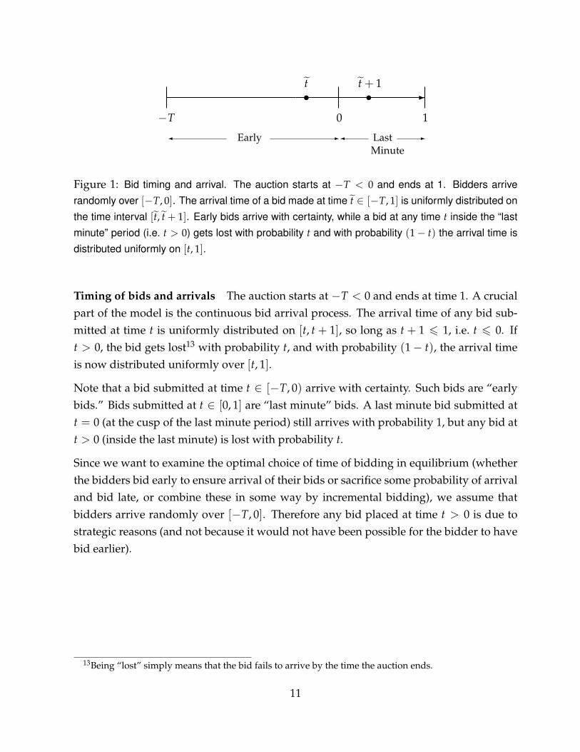
Figure 1: Bid timing and arrival. The auction starts at −T < 0 and ends at 1. Bidders arrive

randomly over [−T, 0]. The arrival time of a bid made at time t ∈ [−T, 1] is uniformly distributed on

the time interval [t, t + 1]. Early bids arrive with certainty, while a bid at any time t inside the “last

minute” period (i.e. t > 0) gets lost with probability t and with probability (1− t) the arrival time is

distributed uniformly on [t, 1].

Timing of bids and arrivals The auction starts at −T < 0 and ends at time 1. A crucialpart of the model is the continuous bid arrival process. The arrival time of any bid sub-mitted at time t is uniformly distributed on [t, t + 1], so long as t + 1 6 1, i.e. t 6 0. Ift > 0, the bid gets lost13 with probability t, and with probability (1− t), the arrival timeis now distributed uniformly over [t, 1].

Note that a bid submitted at time t ∈ [−T, 0) arrive with certainty. Such bids are “earlybids.” Bids submitted at t ∈ [0, 1] are “last minute” bids. A last minute bid submitted att = 0 (at the cusp of the last minute period) still arrives with probability 1, but any bid att > 0 (inside the last minute) is lost with probability t.

Since we want to examine the optimal choice of time of bidding in equilibrium (whetherthe bidders bid early to ensure arrival of their bids or sacrifice some probability of arrivaland bid late, or combine these in some way by incremental bidding), we assume thatbidders arrive randomly over [−T, 0]. Therefore any bid placed at time t > 0 is due tostrategic reasons (and not because it would not have been possible for the bidder to havebid earlier).

13Being “lost” simply means that the bid fails to arrive by the time the auction ends.

11

2.1 Strategy of bidders

A bidder arriving at time s ∈ [−T, 0] can bid one or more (finite number of) bids overtime t ∈ [s, 0]. Further, a bidder can also submit a bid at some point inside the “lastminute,” i.e. at some point q ∈ (0, 1) which then reaches with probability (1− q). Notethat given the continual improvement of technology and connection speeds, the “lastminute” represented here by the unit interval should be thought of as representing ashort period of time over which the bidder can choose to make a bid which might fail toarrive.

For any t ∈ [−T, 1], let ht denote the public history of auction prices up to (but not includ-ing) time t. When the first bid above the reserve price arrives, the reserve price becomesactive.14 Note that the public history ht is thus a step function over the interval [−T, t).

Upon arriving at the auction at s, a bidder can observe ht for all t > s. At any t > s bidderalso observes own valuation, arrival time, as well as the history of own bids up to t. Thesealong with the public history ht form a bidder’s private history at t.

At every instant t, a bidder’s feasible set of actions is to either remain inactive or beactive and submit a bid higher than the current auction price. A strategy of a bidder is asequence of maps, for each time t, from the bidder’s private history to the set of feasibleactions.

Note that types below R0 never win. Further, since type R0 necessarily gets a 0 payoff, it isindifferent across all bid-times. Since we cannot possibly impose any equilibrium restric-tions on the bid-time choice of type R0, we simply break indifference of type R0 in favorof non-participation so that only types v > R0 (types with a strictly positive expectedsurplus) participate, and derive results about the bidding behavior of participating types(R0, v].

14In some auctions, this may not be the case. The first activity that is registered in that case is when thesecond bid above the reserve price arrives. We assume the other variation as the more general one, butnothing in our analysis depends on whether the first activity occurs when the first or second bid above thereserve price arrives.

12

2.2 Strategy of the seller

Next, consider the strategy of the seller. The seller starts with a reserve price of R0. Thisis the seller’s optimal reserve price given the prior information on the distribution fromwhich bidders draw values.

The starting reserve price is part of the stated mechanism. The strategy of the seller refersto submission of shill bids. We assume upfront that the seller submits bids through afinite number of agents and the number of shill bids that can be submitted over the timeinterval [0, 1] is finite.15

In general, the strategy of the seller is similar to that of any buyer. At any time t the sellerobserves the public history ht defined above. The seller also observes the history of ownbids up to t. These form the seller’s private history at t.

At every instant t, a seller’s feasible set of actions is to either remain inactive or be activeand submit a shill bid higher than the current auction price. A strategy of the seller is asequence of maps, for each time t, from the seller’s private history to the set of feasibleactions.

Note that history at time t consists of a set of discrete instants of time at which eitherthe auction became active (reserve price was met) or the auction price jumped. At allother times the auction was inactive. Proposition 1 below shows that the seller optimallysubmits shill bids only when some activity occurs (either reserve met or auction pricejumps). This result is useful in understanding how bidders behave in equilibrium.

Proposition 1. Let any time t be called “active” if either the reserve price is met at t or the pricein the auction changes at t. All other times are called “inactive.” In any equilibrium, the sellersubmits shill bids only at active times.

Proof: Suppose there is an equilibrium in which the seller’s strategy involves submittinga shill bid S at some time t even if no bids arrive until t (so that the reserve price is notmet at t, i.e. there is no discernible activity in the auction). Let R1 be the first shill bid theseller makes when the reserve price is met. We consider two separate cases, S = R1 andS > R1.

15The seller presumably operates through a number of agents - submitting several bids through multipleaccounts from the same IP address can be detected by auction platforms.

13

Consider first the case when S > R1. For this to be the seller’s optimal response at time t,it must be that given no bids arrive until time t, the seller’s belief puts higher weight onhigher valuation distributions compared to the initial belief.16 We now show that suchbeliefs cannot be part of any equilibrium.

For such beliefs to be part of an equilibrium, they must be consistent with the bidders’strategies. Specifically, it must be true that in equilibrium lower valuation bidders bidearlier than higher valuation bidders so that non-arrival of any bid by time t signals ahigher probability of higher values compared to the prior.

However, in that case the strategies of the higher types are not best responses. Note thatsince bidders arrive randomly up to time 0, for any t ∈ [−T, 1) a history with no bidsarriving until t can occur with strictly positive probability.17 A profitable deviation forhigher types is to pool with lower types, since, by following the strategy of the lowertypes the higher types can reduce the probability of facing the shill bid S. This constitutesa profitable deviation from their supposed equilibrium strategies. Therefore the sellerbidding S > R1 when no bids have arrived cannot be part of an equilibrium.

Consider now the situation where no bid has arrived till time t (and hence the reserveprice has not been met) and the seller chooses to submit a shill bid S = R1. For this to beoptimal, the seller’s updated beliefs must be the same upon observing arrival of a bid asalso upon observing non-arrival of any bid .18 However, if it is optimal to submit shill bidS – in effect, increase the reserve price from R0 – irrespective of history the seller observes,then that contradicts the fact that the original reserve price R0 was optimally chosen.

The argument that the seller does not shill bid at any inactive time is similar and weskip the details. Essentially, if it is optimal for the seller to submit a shill bid at anyinactive time t, that would imply either that the strategies of some bidder types are notbest responses or that the action chosen by the seller at the last active time before time twas not optimally chosen.‖

16In other words, the seller attaches a higher probability to higher values being drawn compared to theprior belief.

17No bidder with a value above R0 might arrive. This happens with strictly positive probability. Further,for any t < 1, any bidder with type above R0 might arrive in (t − 1, 0) and so even if such a type bidsimmediately after arrival the bid does not reach by t with strictly positive probability.

18Note that for the seller’s updated beliefs to be the same for these two events, it is a necessary conditionthat the high and the low bidders do not pool.

14

The result shows that the seller submits shill bids only at active times, and for the pur-pose of shill bidding we can ignore inactive times. Note that the seller’s strategy has a“Markovian” property that comes naturally from repeated round of Bayesian updating:the mapping from seller’s private history to actions could alternatively be characterizedas mapping from the (cartesian product of the) seller’s updated beliefs and current priceto actions. The updated belief incorporates all the useful information from past pricechanges and past shill bids.

3 Monotonicity

For some of the results, we need to introduce a further restriction on strategies. This isintroduced below.

Definition 1. (Monotonicity) A strategy of a bidder of type v is monotonic if the followingproperty holds: if the bidder submits a bid of v′ 6 v at time t if the auction price at t is p < v′,then the bidder also submits the bid for any other auction price p′ ∈ (p, v′].

This essentially rules out strategies that involve bidding at some point of time t if pricedoes not exceed p, but refraining from bidding if it does exceed p. Monotonicity hasthe following useful implication. Suppose in some proposed equilibrium, a bidder (saybidder 1) is supposed to submit a bid at time t. Suppose bidder 1 deviates and submits thebid at t′ > t. Monotonicity implies that this deviation cannot strictly increase the chanceof a bid (by some other bidder) being triggered at any future point of time. The later bidweakly reduces the chance of the auction price crossing any given threshold, which inturn weakly delays the next bid being triggered, which again weakly reduces the chanceof the auction price crossing any threshold and so on. Assuming monotonicity gives usthe following results .

Proposition 2. Suppose bidders other than 1 use monotonic strategies. In any equilibrium, forbidder 1 of any type v > R0, bidding at t < 0 is suboptimal.

Proof: From Proposition 1 we know that in any equilibrium the seller’s strategy involvessubmitting a shill bid only at active times (i.e. times when the auction reserve price ismet or auction price jumps). It follows that if the bid-arrival-time distribution shifts tothe right, the distribution of shill bidding times also shifts to the right, which strictly re-

15

duces the probability of successful arrival of shill bids and strictly improves the expectedsurplus of any serious bidder.

Now suppose there is an equilibrium in which some types of bidders submit bids beforetime 0. Suitably rename bidders so that bidder 1 of type v > R0 is among these, andsubmits a serious bid of v′ (a bid that exceeds the current auction price if the reserve pricehas already been met, or exceeds the reserve price if the auction is not yet active) at timet < 0. Consider a deviation by bidder 1 in which the bid of v′ is submitted at time 0. Inboth cases the bid arrives with certainty before the end of the auction. So the deviationdoes not lose any probability of arrival. Further, as discussed above, the assumptionof monotonicity implies that, starting from an equilibrium strategy, if a bidder deviatesand bids later, this cannot increase the chance of a bid by some other bidder type beingtriggered at any future point of time. It follows that shifting bidder 1’s bidding time to0 shifts the bid-arrival-time distribution to the right, which raises bidder 1’s expectedsurplus. Therefore the deviation is profitable, which is a contradiction.‖

The result shows that if there is any equilibrium in which some types bid early, it must bethat bidders use non-monotonic strategies. As discussed in the introduction, this essen-tially involves using strategies that threaten to bid early if the auction price is lower thansome threshold at some point t < 0 (this is a threat because early bids trigger shill bidsearly with greater probability) but delay bidding if auction price crosses the threshold att. In effect others must say to each early-bidding-type: bid early or face a higher probabil-ity that we will bid early. Such threats would work so long the shill bidding consequenceof the punishment is worse than that from conforming. Note that, as discussed before,the seller cannot do anything to induce early bidding. The bidders themselves must usenon-monotonic strategies to threaten each other to sustain early bidding. Once we ruleout non-monotonic strategies, such threats are removed, which is sufficient to remove thepossibility of early bidding.

Let us now show that if others use monotonic strategies, a bidder’s best response cannotinvolve incremental bidding. Proposition 2 rules out bidding before time 0 in this case.However, this still leaves open the possibility that a bidder submits a bid at time 0 andanother inside the “last minute.” So a bidder with value v (say) can submit a bid v1 at time0 and v2 at time q ∈ (0, 1) where v1 < v2 6 v. The next result shows that such incrementalbidding is suboptimal. The bidder should bid either only at 0 or only at some q ∈ (0, 1).

16

Proposition 3. Suppose bidders other than 1 use monotonic strategies. In any equilibrium, forbidder 1 of type v > R0, it is optimal to submit a single bid of v either at time 0 or at some pointof time q ∈ (0, 1). In other words, incremental bidding is suboptimal, and in any equilibrium abidder bids exactly once, and submits a truthful bid, at some point of time in [0,1).

The formal proof is in the appendix. The idea is quite simple: if v1 is a winning bid,adding a bid later can only reduce expected payoff. This is because the bid of v1 arriveswith certainty - so the second bid adds nothing to arrival probability. However, the sec-ond bid arrives before the first bid with strictly positive probability, and when it does,with strictly positive probability it triggers a shill bid. But this shill bid is triggered earlierthan necessary (i.e. earlier than the time at which v1 arrives), thus raising the probabilitythat the shill bid actually arrives, which in turn reduces expected payoff. Thus if it isoptimal not to sacrifice any probability of bid reaching, it is best to bid v at 0 and noth-ing further. If, on the other hand, it is optimal to sacrifice some probability of winning,it is best to bid v at some q > 0. In this case adding a bid of v1 at 0 reduces payoff, as,with strictly positive probability, it arrives earlier than the arrival time of the bid at q andtriggers a shill bid.

4 The main results

First, we rule out the possibility of an equilibrium in which bidders wait beyond time 0to submit bids. This implies that in any equilibrium, bidders do not sacrifice probability-of-bid-arrival in order to snipe the shill bidder. Further, standard weak dominance argu-ments imply that a bidder must submit a truthful bid (i.e., a bid equal to true valuation).It follows then that despite the presence of shill bidding, the auction is efficient “at thetop”: whenever the object is allocated to a genuine bidder, it goes to the highest valuebidder. Further, since the shill bids might not arrive, the auction might even have greaterefficiency “at the bottom”: fewer types may be excluded compared to the auction withoutshill bidding. It follows that under private values, the case against shill-bidding is weakerthan one might expect.

Proposition 4. There is no equilibrium in which any type of any bidder bids after 0.

Proof: Suppose there is an equilibrium in which some type v of some bidder is supposedto bid at time t > 0 under some history. Note that the expected payoff of the bidder con-

17

ditional on the bid arriving at time s > t depends only on s. The time of bid submission isnot part of public history, so the continuation histories conditional on the bid arriving ats are exactly the same whether the bid is submitted at t or some other t′.19 Let π(s) be theexpected payoff conditional on the bid reaching at s.20 Also, note that a bid at t arriveswith probability (1− t). The expected payoff in the purported equilibrium can then bewritten as

P(t) = (1− t)∫ 1

tπ(s)

11− t

ds =∫ 1

tπ(s)ds.

Now consider a deviation to bidding at an earlier time t− ∆ > 0. As noted above, givenany arrival time s > t, the payoff is the same as before. Therefore

P(t− ∆)− P(t) =∫ t

t−∆π(s)ds

Now consider the expected payoff π(s) for any arrival time s ∈ [t− ∆, t). The worst casefor bidder 1 is when such a deviation is detectable with certainty.21 In that case, the worstpossible punishment is that other bidders all bid v at s.22 Since bidder 1 bids at mostown value v, the expected payoff π(s) cannot be negative for any value of s. Further,with strictly positive probability no other bidder draws a value above R0, and even whensome others do draw values above R0, with strictly positive probability no such bid ofv arrives. Similarly, the worst shill bid - a shill bid strictly greater than v - fails to reachwith strictly positive probability. Thus the payoff is always nonnegative, and is strictlypositive with strictly positive probability. Since this is true in the worst case, this is truefor all cases. It follows that for any arrival time s ∈ [t − ∆, t), π(s) > 0. Therefore,P(t− ∆)− P(t) > 0, and the deviation is beneficial, which gives us a contradiction. Thiscompletes the proof.‖

19Bidding at t or t′ would result in different probabilities that the bid reaches at any given s > max{t, t′}but conditional on the bid reaching at s, the expected payoff of the bidder would be exactly the same.

20The realized payoff depends on the history at time s and the subsequent future histories following thehistory at time s. The expected payoff π(s) is an expectation of the realized payoffs taken with respect toall these histories.

21For example, suppose t is the earliest equilibrium bid time for any bidder, or the equilibrium bid timesare such that no bid is supposed to arrive at any point of time in [t − ∆, t). In such cases, a deviation isdetected with certainty.

22Such a punishment might not be credible, but we are simply showing that even under the worst pos-sible punishment the payoff exceeds zero. Therefore, for any other punishment the payoff exceeds zero aswell.

18

We now prove the main results of the paper.

Theorem 1. There exists an equilibrium in which every arriving bidder of any type v ∈ (R0, v]bids once, and truthfully, at time 0.

To prove this, we consider the best bid-time of bidder 1 of type v when some subset ofother bidders arrive. As we show, the optimal bid-time is invariant across all such subsetsand therefore the result does not rely on any knowledge of the precise number of biddersarriving in the auction by any bidder or the seller.

Proof: Consider the following bidder strategies. All bidders of all types remain inactive –i.e., do not submit any bids – for all histories for t ∈ [−T, 0). At t = 0, and for any history,bidder with valuation v submits a bid equal to v if the auction price at time 0 is less thanv; otherwise the bidder remains inactive. For any t ∈ (0, 1], any bidder with valuationv remain inactive if the history of the bidder is such that the bidder has submitted bidequal to v at time 0. For any history such that the bidder has not submitted bid equal tov at time 0, the bidder immediately submits a bid equal to v if the current auction price isstrictly less than v, and remains inactive if the auction price is (weakly) greater than v.

It is clear that if the above is an equilibrium, the resulting outcome would be that all ar-riving bidders would bid for the first time their value of the object at time t = 0. Hence,the remaining task is to check that the above is indeed an equilibrium. It is obvious thatdeviating and bidding at some time t < 0 is not a profitable deviation. Since the strategiesare monotonic by construction, this follows directly from Proposition 2. Consider now adeviation where a bidder submits an additional bid at some t > 0. Again, since the strate-gies are monotonic by construction, it follows from Proposition 3 that this is unprofitable.Finally, It follows from Proposition 4 that deviating and bidding at some time t > 0 isunprofitable. This completes the proof.‖

Next, we consider uniqueness. Let us refer to the time at which bids are submitted inequilibrium as the “equilibrium outcome.” We now show the following.

Theorem 2. If we restrict attention to monotonic strategies, all bidders of all types above R0

bidding at time 0 is the unique equilibrium outcome.

Proof: Proposition 2 rules out bid times before time 0. From Proposition 3, we know thatbidders submit truthful bids once either at 0 or at some point of time in (0, 1). Finally,

19

Proposition 4 rules out the latter. Therefore all types above R0 of all bidders bidding attime 0 is the unique equilibrium outcome.‖

The general properties below follow immediately from the results above.

Proposition 5. Any equilibrium that involves bidding earlier than time 0 must involve non-monotonic strategies by some types (above R0) of some bidders. For the bidders, any such equilib-rium is Pareto dominated compared to an equilibrium where all bidders of all types (above R0) bidat time 0.

Proof: The first part follows directly from Proposition 4. Next, suppose there is an equi-librium in non-monotonic strategies in which some types above R0 of some bidders bidbefore time 0 in equilibrium. This results in the seller’s shill bids being triggered earlierthan an equilibrium in which all types above R0 bid at time 0. Since all bids at time 0 orearlier reach with certainty, bidding before 0 confers no benefits to the bidders, but sinceshill bids arrive with strictly higher probability when bids reach early, the equilibrium innon-monotonic strategies generates a strictly lower expected payoff for all serious typesof all bidders. This completes the proof.‖

5 Conclusion

Last minute bidding is a widely observed phenomenon in online auctions, many of whichfit the private values model well. We provide an explanation for such bidding behaviorthat does not rely on any discontinuity of the bid arrival process. We allow a continuouschoice of bid times and a continuous arrival process for submitted bids. The frameworkcan also be useful for analyzing online auctions under common values or other richervaluation environments. Indeed, some of the results in the literature that depend on anassumption of discontinuity unravel in a continuous framework.

In our model, bidders’ private values are correlated, implying that shill bidding is usefulsince it essentially allows the seller to adjust the reserve price mid-auction.23 As we show,

23In our model shill bids are used to update reserve prices. As noted before, under independent privatevalues, shill bids are irrelevant and there is no reason for bidders to delay their bids either. Other reasons forlate bidding can arise even under independent private values drawn from a known distribution if bids can

20

the seller can only react when the auction registers activity. This in turn implies thatbidders have an incentive to delay events that lead to the seller learning about the valuedistribution, reducing the chance of successful shill bids. In other words, bidders bid latenot because they want to snipe other bidders, but the shill bidder.

Our result shows that all bidders bidding at the last point of time at which their bid stillreaches with probability 1 constitutes an equilibrium. The equilibrium is Pareto dominantfor bidders. Further, we show that the equilibrium bid time is unique if we restrict atten-tion to monotonic strategies. Unlike much of the literature, knowledge of actual numberof bidders is immaterial for our results. We can therefore allow for random entry, so thatneither bidders nor the seller know the precise number of bidders - a setting natural foronline auctions.

As noted in the introduction, shill bidding is illegal and universally frowned on. Theliterature on shill bidding in common value auctions justify such status by showing howshill bids might reduce the seller’s payoff in equilibrium by impeding information aggre-gation. However, our results suggest that the case against shill bidding is much weakerunder private values. We show that there are no equilibria that involve bidding later thantime 0. An implication of this is that in all equilibria, when the object is sold to a genuinebidder, it goes to the bidder with the highest value. Therefore there is no efficiency loss“at the top.” Further, the option of shill bidding might lead the seller to post a lower initialreserve price compared to the case where such an option is not available.24 Subsequently,given sniping by bidders, some or all updates might not arrive, making the auction withshill bids more efficient ex post compared to auctions without shill bidding.

The auction we consider has a fixed end time. We can also consider efficiency compar-isons with auctions that have a flexible end time. In the latter, all shill bids necessarily

be cancelled after submission. For example the seller might attempt the following: submit a high shill bidto discover the highest genuine bid, cancel the high shill bid and submit instead a shill bid just below thehighest genuine bid (essentially trying to extract the first price in a second-price auction). In such situations,it is reasonable to suppose that the bidders will, in turn, delay submitting their bids in order to delay value-discovery and snipe the seller’s shill bids. While a full blown analysis of such alternative motives for latebidding is beyond the scope of the paper, it is possible that the resulting outcome would be similar to theequilibrium outcome from our model, namely that the bidders would delay bid-submission to lower thechance of successful shill bids, but not delay to an extent that would involve sacrificing any probability oftheir own bid arriving before the auction closes.

24Such cases are likely when, for example, the prior over distributions puts sufficient weight on bothlower (in stochastic dominance ranking) and higher distributions.

21

reach. On the other hand, the initial reserve price would be lower than that under a fixedend-time auction. Thus there are two conflicting effects. A flexible end-time auction offersa lower initial reserve price but all shill bids reach, so it is possible that the seller “over-shoots,” i.e. submits a shill bid that is too high relative to the optimal reserve price if thetrue distribution were known. A fixed-end time auction may have a higher reserve price,but the shill bids might not reach, so it suffers less from the overshooting problem. Onemight conjecture that given distributions ranked by first-order stochastic dominance, ifthe bidders are from a distribution with low mean, they would gain from a flexible end-time auction relative to a fixed end-time one, as the lower initial reserve price effect islikely to outweigh the overshooting effect. Similarly, bidders from high mean distribu-tions are likely to prefer fixed end-time auctions. The highest mean distribution is likelyto face a higher expected reserve price under a flexible end-time auction compared to afixed end-time one.

Which auction is better for the seller? While this is beyond the scope of our analysis, webelieve that the key to this lies in entry incentives. Since, ceteris paribus, buyers froma higher distribution are likely to obtain more surplus from auctions with a fixed end-time, such an auction would be more attractive to them, and less attractive to the seller.However, with endogenous buyer entry, buyers from a high distribution might self-selectinto a fixed-end-time auction, and then it is not clear that a flexible end-time auction nec-essarily generates more expected revenue for the seller. Studying competition amongstonline auction sites using different auction mechanisms in environments characterizedby endogenous entry by buyers and sellers should be an interesting and important topicfor future research.

22

Appendix

A.1 Proof of Proposition 3

Consider the problem of bidder 1 of type v. Consider an incremental bidding strategy v1

at time 0 and v2 at time q ∈ (0, 1), where v1 < v2 6 v.

In what follows, the term “positive probability” means probability strictly greater thanzero.

Step 1: Let P0(v1, v2) be the expected payoff given that v1 is a winning bid and giventhat v1 reaches.

Since v1 reaches with certainty, the bid of v2 serves in this case only to trigger a shill bidearlier than necessary with positive probability. To see this, suppose v1 arrives at t > q(an event that occurs with positive probability). In the absence of the bid of v2 at q, ashill bid would be triggered by bidder 1’s bid only at t. However, if the bid of v2 arrivesbefore t (which happens with positive probability), a shill bid is triggered earlier thannecessary (note that an earlier shill bid has a greater chance of reaching, thereby reducingthe expected payoff of bidder 1). Further, monotonicity of strategies of bidders other than1 implies that if a bid from 1 arrives later, this cannot increase the chance of a bid (by someother bidder) being triggered at any future point of time. Therefore dropping the bid atq must also weakly delay the shill bids triggered by arrival of bids by other bidders. Itfollows that the payoff given v1 is a winning bid can be improved by dropping the bid atq:

P0(v1, v2) < P0(v1). (A.1)

Here P0(v1) is the expected payoff of bidder 1 given v1, submitted at time 0, wins (andthere are no other bids).

Next, note that if v1 is a winning bid, so is any bid greater than v1. In particular, v is awinning bid. Further, if we raise v1, the payoff given v1 wins does not change. This isa standard property of second price auctions - raising the winning bid does not changeauction price (in other words, any higher bid is observationally equivalent: it has thesame impact on auction price and triggers shill bids in exactly the same way). So the

23

payoff given v1 wins (P0(v1)) is the same as the payoff given v wins, i.e.

P0(v1) = P0(v). (A.2)

Step 2: Next, let EPq(v1, v2) denote the expected payoff when v1 is a losing bid and v2

reaches. Note that v2 gets lost with positive probability - so the bidder’s expected payoffis a product of the actual expected payoff given v2 wins and v1 loses, and the probabilityof arrival of the bid of v2.

Now, if v2 < v, EPq(v1, v2) can be raised by setting v2 = v since when v2 wins, whetherv2 < v or v2 = v makes no difference to payoff, but in cases where v2 loses and v wins,the payoff gets raised. It follows that

EPq(v1, v2) 6 EPq(v1, v). (A.3)

Step 3: The expected payoff from the incremental bidding strategy is given by:

πinc = Pr(v1 wins)P0(v1, v2) + Pr(v1 loses, v2 wins)EPq(v1, v2).

Using the inequalities (A.1) to (A.3),

πinc < π = Pr(v1 wins)P0(v) + Pr(v1 loses, v wins)EPq(v1, v).

Next, let

α(v1) =Pr(v1 wins)Pr(v wins)

.

Note that as v1 → v, α → 1. Also, if v1 is dropped (or, equivalently, v1 is set to a valuelower than the initial reserve price R0), α = 0. For the purpose of the proof, let us repre-sent dropping v1 as setting v1 = 0. Then v1 ∈ {0} ∪ [R0, v]. Further, if v1 is raised to v,α = 1. Then we can write

π = Pr(v wins)[

α(v1)P0(v) + (1− α(v1))EPq(v1, v)]

(A.4)

If we can show that the convex combination inside the square brackets is maximizedeither if v1 = 0 or v1 = v, that would prove that incremental bidding is suboptimal andthe optimal strategy is either to bid only at 0 or to bid only at some point q > 0. Further,since bidding exactly once is optimal, the optimal bid is indeed v. This would completethe proof.

24

We now show that the convex combination inside the square brackets is indeed maxi-mized at a corner.

Consider the term inside the square brackets. As v1 decreases, α decreases. Further,the payoff given v1 is a losing bid (EPq(v1, v)) increases. This is because the bid of v1,which reaches with certainty, reaches before the winning bid with positive probability,and therefore triggers shill bids earlier than necessary (i.e. earlier than shill bids triggeredby arrival of the winning bid) with positive probability. A lower v1 still reaches before thewinning bid with the same probability, but upon reaching triggers a shill bid with lowerprobability, thereby raising payoff.

It follows that the payoff given v1 is a losing bid and v arrives is maximized when v1 isdropped altogether:

EPq(v1, v) < EPq(v) (A.5)

Consider the convex combination α(v1)P0(v) + (1− α(v1))EPq(v1, v). As specified above,v1 ∈ {0} ∪ [R0, v], where v1 = 0 represents dropping the bid of v1. As v1 varies, P0(v)does not change while EPq(v1, v) is strictly decreasing in v1.

The two corner values of the convex combination are P0(v) and EPq(v), corresponding tov1 = v and v1 = 0 respectively. Now suppose there is an interior value of v1 (i.e. somev1 ∈ [R0, v)) that maximizes the convex combination. For that interior value, we haveα(v1)P0(v) + (1− α(v1))EPq(v1, v) > max[P0(v), EPq(v)], or writing it out, we have,

α(v1)P0(v) + (1− α(v1))EPq(v1, v) > P0(v), (A.6)

α(v1)P0(v) + (1− α(v1))EPq(v1, v) > EPq(v). (A.7)

Since 1− α(v1) 6= 0, we have from (A.6) that

P0(v) 6 EPq(v1, v). (A.8)

From (A.7), we have

α(v1)(P0(v)− EPq(v1, v)) > EPq(v)− EPq(v1, v) > 0,

where the last inequality follows from (A.5). Since v1 is an interior point, we have α(v1) >

0. Therefore, the above implies P0(v) > EPq(v1, v), which contradicts (A.8).

It follows that the expression α(v1)P0(v) + (1− α(v1))EPq(v1, v) cannot be maximized atan interior value of v1 - it is maximized either by bidding only at 0 or by bidding only

25

at some point q > 0. Therefore incremental bidding is suboptimal, and the only relevantquestion is whether the bidder should bid at 0 or wait until some point q > 0 to bid.Since bidding exactly once is optimal, it also follows from standard second-price auctionlogic that truthful bidding is optimal (bidding anything other than true value is weaklydominated). This completes the proof.‖

26

References

Bajari, Patrick and Ali Hortacsu, “The Winner’s Curse, Reserve Prices, and EndogenousEntry: Empirical Insights from eBay Auctions,” Rand Journal of Economics, 2003, 34 (2),329–355. 1, 7

Chakraborty, Indranil and Georgia Kosmopoulou, “Auctions with shill bidding,” Eco-nomic Theory, 2004, 24, 271–287. 8

Engelberg, Joseph and Jared Williams, “eBays proxy bidding: A license to shill,” Journalof Economic Behavior and Organisation, 2009, 72, 509–526. 8

Lamy, Laurent, “The Shill Bidding Effect versus the Linkage Principle,” Journal of Eco-nomic Theory, 2009, 144, 390–413. 8

Myerson, Roger, “Optimal Auctions,” Mathematics of Operations Research, 1981, 6, 58–63.3

Ockenfels, Axel and Alvin E. Roth, “Late and multiple bidding in second price Internetauctions: Theory and evidence concerning different rules for ending an auction,” Gamesand Economic Behavior, 2006, 55, 297–320. 1, 6, 7, 8

Rasmusen, Eric Bennett, “Strategic Implications of Uncertainty over One’s Own PrivateValue in Auctions,” Advances in Theoretical Economics, B E Journal of Theoretical Economics,2006, 6 (1). 8

Roth, Alvin E. and Axel Ockenfels, “Last-Minute Bidding and the Rules for EndingSecond-Price Auctions: Evidence from eBay and Amazon Auctions on the Internet,”American Economic Review, 2002, 92 (4), 1093–1103. 1, 7

The Sunday Times, “Revealed: how eBay sellers fix auctions,” 2007. January 28. 3

Walton, Kenneth, Fake: Forgery, Lies, & eBay, Gallery Books, 2006. 3

Whitworth, Dan, “Man fined over fake eBay auctions (BBC Newsbeat),” 2010. July 5. 3

Wintr, Ladislav, “Some Evidence on Late Bidding in eBay auctions,” Economic Inquiry,2008, 46 (3), 369–379. 1

27