Several Variable Differential Calculus

1 Motivations

The aim of studying the functions depending on several variables is to understand the

functions which has several input variables and one or more output variables. For example,

the following are Real valued functions of two variables x, y:

(1) f(x, y) = x2 + y2 is a real valued function defined over IR2.

(2) f(x, y) = xyx2+y2

is a real valued function defined over IR2\{(0, 0)}The real world problems like temperature distribution in a medium is a real valued function

with more than 2 variables. The temperature function at time t and at point (x, y) has

3 variables. For example, the temperature distribution in a plate, (unit square) with zero

temperature at the edges and initial temperature (at time t = 0)T0(x, y) = sin πx sin πy, is

T (t, x, y) = e−π2kt sin πx sin πy.

Another important problem of physics is Sound waves and water waves. The function

u(x, t) = A sin(kx − ωt) represents the traveling wave of the initial wave front sin kx.

The Optimal cost functions, for example a manufacturing company wants to optimize the

resources, for their produce, like man power, capital expenditure, raw materials etc. The

cost function depends on these variables. Earning per share for Apple company (2005-

2010) has been modeled by z = 0.379x − 0.135y − 3.45 where x is the sales and y is the

share holders equity.

2 Limits

Let IR2 denote the set of all points (x, y) : x, y ∈ IR. The open ball of radius r with center

(x0, y0) is denoted by

Br((x0, y0)) = {(x, y) :√(x− x0)2 + (y − y0)2 < r}.

Definition: A point (a, b) is said to be interior point of a subset A of IR2 if there exists r

such that Br((a, b)) ⊂ A. A subset Ω is called open if each point of Ω is an interior point

of Ω. A subset is said to be closed in its compliment is an open subset of IR2. For example

(1). The open ball of radius δ: Bδ((0, 0)) = {(x, y) ∈ IR2 : x2 + y2 < 1} is an open set

1

(2). Union of open balls is also an open set.

(3). The closed ball of radius r : Br((0, 0)) = {(x, y) :√|x|2 + |y|2 ≤ r} is closed.

A sequence {(xn, yn)} is said to converge to a point (x, y) in IR2 if for ε > 0, there exists

N ∈ IN such that √|xn − x|2 + |yn − y|2 < ε, for all n ≥ N.

Definition: Let Ω be a open set in IR2, (a, b) ∈ Ω and let f be a real valued function

defined on Ω except possibly at (a, b). Then the limit lim(x,y)→(a,b)

f(x, y) = L if for any ε > 0

there exists δ > 0 such that

√(x− a)2 + (y − b)2 < δ =⇒ |f(x, y)− L| < ε.

Using the triangle inequality (as in one variable limit), one can show that if limit exists,

then it is unique. That is, the limit is independent of choice path (xn, yn)→ (a, b).

1. Examples

(a) Consider the function f(x, y): f(x, y) =4xy2

x2 + y2. This function is defined in

IR2\{(0, 0)}. Let ε > 0. Then 4|xy2| ≤ 2(x2 + y2)(√x2 + y2). Therefore δ = ε

For such δ, |f(x, y)− 0| < ε

Figure 1:

(b) Finding limit through polar coordinates

Consider the function f(x, y) =x3

x2 + y2. This function is defined in IR2\{(0, 0)}.

2

Taking x = r cos θ, y = r sin θ, we get

|f(r, θ)| = |r cos3 θ| ≤ r → 0 as r → 0.

Figure 2:

2. Example of function which has different limits along different straight lines.

Consider the function f(x, y) f(x, y) =xy

x2 + y2. Then along the straight lines y =

mx, we get f(x,mx) = m1+m2 . Hence limit does not exist.

Figure 3:

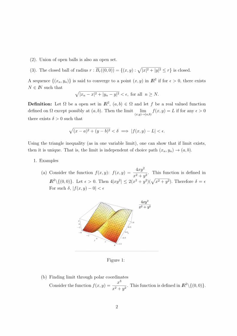
3. Example function where polar coordinates seem to give wrong conclusions

Consider the function f(x, y) =2x2y

x4 + y2. Taking the path, y = mx2, we see that the

3

limit does not exist at (0, 0). Now taking x = r cos θ, y = r sin θ, we get

f(r, θ) =2r cos2 θ sin θ

r2 cos4 θ + sin2 θ.

For any r > 0, the denominator is > 0. Since | cos2 θ sin θ| ≤ 1, we tend to think for

Figure 4:

a while that this limit goes to zero as r → 0. So if we take the path r sin θ = r2 cos2 θ,

(i.e., r = sin θcos2 θ

), we get

f(r, θ) =2 sin2 θ

2 sin2 θ= 1.

3 Continuity and Partial derivatives

Let f be a real valued function defined in a ball around (a, b). Then

Definition: f is said to be continuous at (a, b) if

lim(x,y)→(a,b)

f(x, y) = f(a, b)

4

Example: The function

f(x, y) =

⎧⎨⎩

xy√x2+y2

x2 + y2 = 0

0 x = y = 0

Let ε > 0. Then |f(x, y)− 0| = |x| |y|√x2+y2

≤ |x|. So if we choose δ = ε, then |f(x, y)| ≤ ε.

Figure 5:

Therefore, f is continuous at (0, 0).

Partial Derivatives: The partial derivative of f with respect to x at (a, b) is defined as

∂f

∂x(a, b) = lim

h→0

1

h(f(a+ h, b)− f(a, b)) .

similarly, the partial derivative with respect to y at (a, b) is defined as

∂f

∂y(a, b) = lim

k→0

1

k(f(a, b+ k)− f(a, b)) .

Example: Consider the function

f(x, y) =

⎧⎨⎩

xyx2+y2

(x, y) ≡ (0, 0)

0 (x, y) ≡ (0, 0)

5

As noted earlier, this is not a continuous function, but

fx(0, 0) = limh→0

f(h, 0)− f(0, 0)

h= lim

h→0

0− 0

h= 0.

Similarly, we can show that fy(0, 0) exists.

Also for a continuous function, partial derivatives need not exist. For example f(x, y) =

Figure 6:

|x|+ |y|. This is a continuous function at (0, 0). Indeed, for any ε > 0, we can take δ < ε/2.

But partial derivatives do not exist at (0, 0)

Sufficient condition for continuity:

Theorem: Suppose one of the partial derivatives exist at (a, b) and the other partial

derivative is bounded in a neighborhood of (a, b). Then f(x, y) is continuous at (a, b).

Proof: Let fy exists at (a, b). Then

f(a, b+ k)− f(a, b) = kfy(a, b) + ε1k,

where ε1 → 0 as k → 0. Since fx exists and bounded in a neighborhood of at (a, b),

f(a+ h, b+ k)− f(a, b) =f(a+ h, b+ k)− f(a, b+ k) + f(a, b+ k)− f(a, b)

=hfx(a+ θh, b+ k) + kfy(a, b) + ε1k

≤hM + k|fy(a, b)|+ ε1k

→ 0 as h, k → 0.

6

Directional derivatives, Definition and examples

Let p = p1i + p2j be any unit vector. Then the directional derivative of f(x, y) at (a, b)

in the direction of p is

Dpf(a, b) = lims→0

f(a+ sp1, b+ sp2)− f(a, b)

s.

Example f(x, y) = x2 + xy at P (1, 2) in the direction of unit vector u = 1√2i+ 1√

2j.

Dpf(1, 2) = lims→0

f(1 + s√2, 2 + s√

2)− f(1, 2)

s

= lims→0

1

s

(s2 + s(2

√2 +

1√2)

)= 2√2 +

1√2

The existence of partial derivatives does not guarantee the existence of directional

derivatives in all directions. For example take

f(x, y) =

⎧⎨⎩

xyx2+y2

x2 + y2 = 0

0 x = y = 0.

Let −→p = (p1, p2) such that p21 + p22 = 1. Then the directional derivative along p is

Dpf(0, 0) = limh→0

f(hp1, hp2)− f(0, 0)

h= lim

h→0

p1p2h(p21 + p22)

exist if and only if p1 = 0 or p2 = 0.

The existence of all directional derivatives does not guarantee the continuity of the

function. For example take

f(x, y) =

⎧⎨⎩

x2yx4+y2

(x, y) ≡ (0, 0)

0 x = y = 0.

7

Let −→p = (p1, p2) such that p21 + p22 = 1. Then the directional derivative along p is

Dpf(0, 0) = lims→0

f(sp1, sp2)− f(0, 0)

s

= lims→0

s3p21p2s(s4p41 + s2p22)

=p21p2p22

if p2 = 0

In case of p2 = 0, we can compute the partial derivative w.r.t y to be 0. Therefore all the

directional derivatives exist. But this function is not continuous (y = mx2 and x→ 0).

4 Differentiability

Let D be an open subset of IR2. Then

Definition: A function f(x, y) : D → IR is differentiable at a point (a, b) of D if there

exists ε1 = ε(h, k), ε2 = ε2(h, k) such that

f(a+ hb+ k)− f(a, b) = hfx(a, b) + kfy(a, b) + hε1 + kε2,

where ε1, ε2 → 0 as (h, k)→ (0, 0).

Problem: Show that the following function f(x, y) is is not differentiable at (0, 0)

f(x, y) =

⎧⎨⎩x sin

1x+ y sin 1

y, xy = 0

0 xy = 0

Solution: |f(x, y)| ≤ |x|+ |y| ≤ 2√x2 + y2 implies that f is continuous at (0, 0). Also

fx(0, 0) = limh→0

f(h, 0)− f(0, 0)

h= 0.

fy(0, k) = limk→0

f(0, k)− f(0, 0)

k= 0.

If f is differentiable, then there exists ε1, ε2 such that

f(h, k)− f(0, 0) = ε1h+ ε2k

8

Figure 7:

where ε1, ε2 → 0 as h, k → 0. Now taking h = k, we get

f(h, h) = (ε1 + ε2)h =⇒ 2h sin1

h= h(ε1 + ε2).

So as h→ 0, we get sin 1h→ 0, a contradiction.

Problem: Show that the function f(x, y) =√|xy| is not differentiable at the origin.

Solution: Easy to check the continuity (take δ = ε).

fx(0, 0) = limh→0

0− 0

h= 0, and similar calculation shows fy(0.0) = 0

So if f is differentiable at (0, 0), then there exist, ε1, ε2 such that

f(h, k) = ε1h+ ε2k.

Taking h = k, we get

|h| = (ε1 + ε2)h.

This implies that (ε1 + ε2) → 0.

Notations:

1. Δf = f(a+ h, b+ k)− f(a, b), the total variation of f

2. df = hfx(a, b) + kfy(a, b), the total differential of f .

3. ρ =√h2 + k2

9

Equivalent condition for differentiability:

Theorem: f is differentiable at (a, b) ⇐⇒ limρ→0

Δf − df

ρ= 0.

Proof. Suppose f(x, y) is differentiable. Then, there exists ε1, ε2 such that

f(a+ h, b+ k)− f(a, b) = hfx(a, b) + kfy(a, b) + hε1 + kε2,

where ε1, ε2 → 0 as (h, k)→ (0, 0).

Therefore, we can writeΔf − df

ρ= ε1(

h

ρ) + ε2(

k

ρ),

where df = hfx(a, b) + kfy(a, b) and ρ =√h2 + k2. Now since |h

ρ| ≤ 1, k

ρ≤ 1 we get

limρ→0

Δf − df

ρ= 0.

On the other hand, if limρ→0Δf−df

ρ= 0, then

Δf = df + ερ, ε→ 0 as h, k → 0.

ερ =ερ

|h|+ |k| |h|+ερ

|h|+ |k| |k|

=ερ sgn(h)

|h|+ |k| h+ερ sgn(k)

|h|+ |k| k

Therefore, we can take ε1 =ερ sgn(h)|h|+|k| and ε2 =

ερ sgn(k)|h|+|k| .

Example: Consider the function f(x, y) =

⎧⎨⎩

x2y2

x2+y2(x, y) ≡ (0, 0)

0 x = y = 0.

Partial derivatives exist at (0, 0) and fx(0, 0) = 0, fy(0, 0) = 0. By taking h = ρ cos θ, k =

Figure 8:

10

ρ sin θ, we getΔf − df

ρ=h2k2

ρ3=ρ4 cos2 θ sin θ

ρ3= ρ cos2 θ sin θ.

Therefore,∣∣∣Δf−df

ρ

∣∣∣ ≤ ρ→ 0 as ρ→ 0. Therefore f is differentiable at (0, 0).

Example: Consider f(x, y) =

⎧⎨⎩

x2yx2+y2

(x, y) ≡ 0

0 x = y = 0.

Partial derivatives exist at (0, 0) and fx(0, 0) = fy(, 0) = 0. By taking h = ρ cos θ, k =

ρ sin θ, we getΔf − df

ρ=h2k

ρ3=ρ3 cos2 θ sin θ

ρ3= cos2 θ sin θ.

The limit does not exist. Therefore f is NOT differentiable at (0, 0).

The following theorem is on Sufficient condition for differentiability:

Theorem: Suppose fx(x, y) and fy(x, y) exist in an open neighborhood containing (a, b)

and both functions are continuous at (a, b). Then f is differentiable at (a, b).

Proof. Since ∂f∂y

is continuous at (a, b), there exists a neighborhood N(say) of (a, b) at

every point of which fy exists. We take (a+ h, b+ k), a point of this neighborhood so that

(a+ h, b), (a, b+ k) also belongs to N .

We write

f(a+h, b+k) − f(a, b) = {f(a+h, b+k) − f(a+h, b)} + {f(a+h, b) − f(a, b)}.

Consider a function of one variable φ(y) = f(a+ h, y).

Since fy exists in N, φ(y) is differentiable with respect to y in the closed interval [b, b+ k]

and as such we can apply Lagrange’s Mean Value Theorem, for function of one variable y

in this interval and thus obtain

φ(b+ k) − φ(b) = kφ′(b+ θk), 0 < θ < 1

= kfy(a+ h, b+ θk)

f(a+ h, b+ k) − f(a+ h, b) = kfy(a+ h, b+ θk), 0 < θ < 1.

11

Now, if we write

fy(a+ h, b+ θk) − fy(a, b) = ε2 (a function of h, k)

then from the fact that fy is continuous at (a,b). we may obtain

ε2 → 0 as (h, k)→ (0, 0).

Again because fx exists at (a, b) implies

f(a+ h, b) − f(a, b) = hfx(a, b) + ε1h,

where ε1 → 0 as h→ 0. Combining all these we get

f(a+ h, b+ k) − f(a, b) = k[fy(a, b) + ε2] + hfx(a, b) + ε1h

= hfx(a, b) + kfy(a, b) + ε1h + ε2k

where ε1, ε2 are functions of (h, k) and they tend to zero as (h, k)→ (0, 0).

This proves that f(x, y) is differentiable at (a, b).

Remark: The above proof still holds if fy is continuous and fx exists at (a, b).

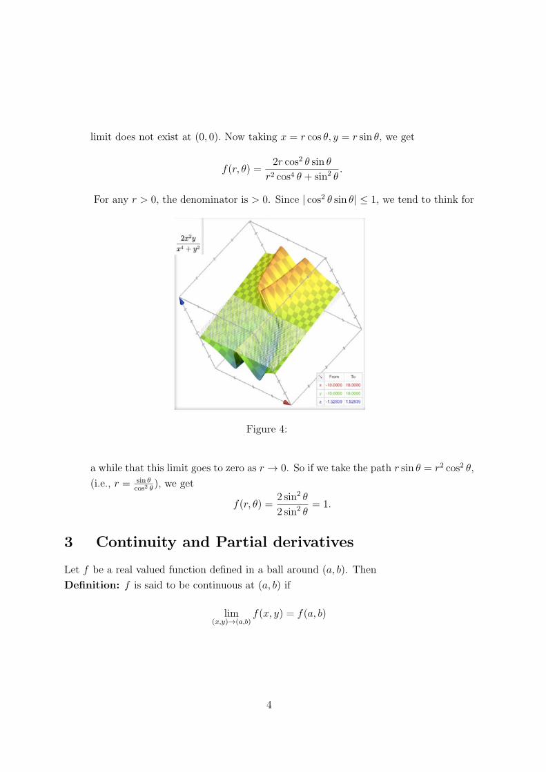
There are functions which are Differentiable but the partial derivatives need not be con-

tinuous. For example, consider the function

f(x, y) =

⎧⎨⎩x

3 sin 1x2 + y3 sin 1

y2xy = 0

0 xy = 0.

Then

fx(x, y) =

⎧⎨⎩3x2 sin 1

x2 − 2 cos 1x2 xy = 0

0 xy = 0

Also fx(0, 0) = limh→0f(h,0)−f(0,0)

h= 0. So partial derivatives are not continuous at (0, 0).

f(Δx,Δy) = (Δx)3 sin1

(Δx)2+ (Δy)3 sin

1

(Δy)2

= 0 + 0 + ε1Δx+ ε2Δy

12

Figure 9:

where ε1 = (Δx)2 sin 1(Δx)2

and ε2 = (Δy)2 sin 1(Δy)2

. It is easy to check that ε1, ε2 → 0. So

f is differentiable at (0, 0).

There are functions for which directional derivatives exist in any direction, but the

function is not differentiable.

Example: Consider the function

f(x, y) =

⎧⎨⎩

y|y|√x2 + y2 y = 0

0 y = 0

(Exercise problem)

Chain rule:

Partial derivatives of composite functions: Let z = F (u, v) and u = φ(x, y), v = ψ(x, y).

Then z = F (φ(x, y), ψ(x, y)) as a function of x, y. Suppose F, φ, ψ have continuous partial

derivatives, then we can find the partial derivatives of z w.r.t x, y as follows: Let x be

increased by Δx, keeping y constant. Then the increment in u is Δxu = u(x + Δx, y) −u(x, y) and similarly for v. Then the increment in z is (as z is differentiable as a function

of u, v )

Δxz := z(x+Δx, y +Δy)− z(x, y) =∂F

∂uΔxu+

∂F

∂vΔxv + ε1Δxu+ ε2Δxv

Now dividing by Δx

Δxz

Δx=∂F

∂u

Δxu

Δx+∂F

∂v

Δxv

Δx+ ε1

Δxu

Δx+ ε2

Δxv

Δx

13

Taking Δx→ 0, we get

∂z

∂x=∂F

∂u

∂u

∂x+∂F

∂v

∂v

∂x+ ( lim

Δx→0ε1)

∂u

∂x+ ( lim

Δx→0ε2)

∂v

∂x

=∂F

∂u

∂u

∂x+∂F

∂v

∂v

∂x

similarly, one can show∂z

∂y=∂F

∂u

∂u

∂y+∂F

∂v

∂v

∂y.

Example: Let z = ln(u2 + v2), u = ex+y2 , v = x2 + y.

Then zu = 2uu2+v

, zv =1

u2+v, ux = ex+y2 , vx = 2x. Then

zx =2u

u2 + vex+y2 +

2x

u2 + v

Derivative of Implicitly defined function

Let y = y(x) be defined as F (x, y) = 0, where F, Fx, Fy are continuous at (x0, y0) and

Fy(x0, y0) = 0. Then dydx

= −Fx

Fyat (x0, y0).

Increase x by Δx, then y receives Δy increment and F (x+Δx, y +Δy) = 0. Also

0 = ΔF = FxΔx+ FyΔy + ε1Δx+ ε2Δy

where ε1, ε2 → 0 as Δx→ 0. This is same as

Δy

Δx= −Fx + ε1

Fy + ε2

Now taking limit Δx→ 0, we get dydx

= −Fx

Fy.

Example: The function y = y(x) as ey − ex + xy = 0. Then Fx = −ex + y, Fy = ey + x.

Then dydx

= ex−yey+x

.

Proposition If f(x, y) is differentiable, then the directional derivative in the direction p

at (a, b)is

Dpf(a, b) = ∇f(a, b) · p.Proof: Let p = (p1, p2). Then from the definition,

lims→0

f(a+ sp1, b+ sp2)− f(a, b)

s= lim

s→0

f(x(s), y(s))− f(x(0), y(0))

s

14

where x(s) = a+ sp1, y(s) = b+ sp2.

From the chain rule,

lims→0

f(x(s), y(s))− f(x(0), y(0))

s=∂f

∂x(a, b)

dx

ds+∂f

∂y(a, b)

dy

ds= ∇f(a, b) · (p1, p2).

Using the directional derivatives, we can also find the Direction of maximum rate of change.

Properties of directional derivative for differentiable function

Dpf = ∇f · p = |∇f | cos θ. So the function f increases most rapidly when cos θ = 1 or

when p is the direction of ∇f . The derivative in the direction ∇f|∇f | is equal to |∇f |.

Similarly, f decreases most rapidly in the direction of −∇f . The derivative in this direction

is Dpf = −|∇f |. Finally, the direction of no change is when θ = π2. i.,e., p ⊥ ∇f .

Problem: Find the direction in which f = x2/2 + y2/2 increases and decreases most

rapidly at the point (1, 1). Also find the direction of zero change at (1, 1).

Example Functions for which all directional derivatives exist but not differentiable.

Consider the function

f(x, y) =

⎧⎨⎩

y|y|√x2 + y2, y = 0

0 y = 0

Dpf(a, b) = lims→0

f(sp1, sp2)− f(0, 0)

s=

p2|p2| .

fx(0, 0) = limh→0

0− 0

h= 0, fy(0, 0) = lim

k→0

k|k|√k2

k= 1.

In this case, both Dpf(a, b) and ∇f(a, b) · p exists but not equal.

Tangents and Normal to Level curves

Let f(x, y) be differentiable and consider the level curve f(x, y) = c. Let −→r (t) = g(t)i +

h(t)j be its parametrization. for example f(x, y) = x2 + y2 has x(t) = a cos t, y(t) = a sin t

as level curve x2 + y2 = a2, which is a circle of radius a. Now differentiating the equation

f(x(t), y(t)) = a2 with respect to t, we get

fxdx

dt+ fy

dy

dt= 0.

Now since −→r ′(t) = x′(t)i+ y′(t)j is the tangent to the curve, we can infer from the above

equation that ∇f is the direction of Normal. Hence we have

Equation of Normal at (a, b) is x = a+ fx(a, b)t, y = b+ fy(a, b)t, t ∈ IREquation of Tangent is (x− a)fx(a, b) + (y − b)fy(a, b) = 0.

15

Example Find the normal and tangent to x2

4+ y2 = 2 at (−2, 1).

Solution: We find ∇f = x2i + 2yj (−2,1) = −i + 2j. Therefore, the Tangent line through

Figure 10:

(−2, 1) is −(x+ 2) + 2(y − 1) = 0.

Tangent Plane and Normal lines

Let −→r (t) = g(t)i + h(t)j + k(t)k is a smooth level curve(space curve) of the level surface

f(x, y, z) = c. Then differentiating f(x(t), y(t), z(t)) = c with respect to t and applying

chain rule, we get

∇f(a, b, c) · (x′(t), y′(t), z′(t)) = 0

Now as in the above, we infer the following:

Normal line at (a, b, c) is x = a+ fxt, y = b+ fyt, z = c+ fzt.

Tangent plane: (x− a)fx + (y − b)fy + (z − c)fz = 0.

Example: Find the tangent plane and normal line of f(x, y, z) = x2 + y2 + z − 9 = 0 at

(1, 2, 4).

∇f+2xi+2yj+k at (1,2,4) is = 2i+4j+k and tangent plane is 2(x−1)+4(y−2)(z−4) = 0.

Figure 11:

Then normal line is x = 1 + 2t, y = 2 + 4t, z = 4 + t.

16

Problem: Find the tangent line to the curve of intersection of two surfaces f(x, y, z) =

x2 + y2 − 2 = 0, z ∈ R, g(x, y, z) = x+ z − 4 = 0.

Solution: The intersection of these two surfaces is an an ellipse on the plane g = 0.

Figure 12:

The direction of normal to g(x, y, z) = 0 at (1, 1, 3) is i+ k and normal to f(x, y, z) = 0 is

2i+2j. The required tangent line is orthogonal to both these normals. So the direction of

tangent is

v = ∇f ×∇g = 2i− 2j − 2k.

Tangent through (1, 1, 3) is x = 1 + 2t, y = 1− 2t, z = 3− 2t.

Linearization: Let f be a differentiable function in a rectangle containing (a, b). The

linearization of a function f(x, y) at a point (a, b) where f is differentiable is the function

L(x, y) = f(a, b) + fx(a, b)(x− a) + fy(a, b)(y − b).

The approximation f(x, y) ∼ L(x, y) is the standard linear approximation of f(x, y) at

(a, b). Since the function is differentiable,

E(x, y) = f(x, y)− L(x, y) = ε1(x− a) + ε2(y − b)

where ε1, ε2 → 0 as x→ a, y → b. The error of this approximation is

|E(x, y)| ≤ M

2(|x− a|+ |y − b|)2.

where M = max{|fxx|, |fxy|, |fyy|}.Example: Find the linearization and error in the approximation of f(x, y, z) = x2− xy+12y2 + 3 at (3, 2).

17

f(3, 2) = 8, fx(3, 2) = 4, fy(3, 2)− 1. So

L(x, y) = 8 + 4(x− 3)− (y − 2) = 4x− y − 2

Also max{|fxx|, |fxy|, |fyy|} = 2 and

|E(x, y)| ≤ (|x− 3|+ |y − 2|)2

If we take the rectangle R : |x− 3| ≤ 0.1, |y − 2| ≤ 0.1.

5 Taylor’s theorem

Higher order mixed derivatives:

It is not always true that the second order mixed derivatives fxy =∂∂x(∂f∂y) and fyx = ∂

∂y(∂f∂x)

are equal. The following is the example

Example: f(x, y) =

⎧⎨⎩

xy(x2−y2)x2+y2

, x = 0, y = 0

0 x = y = 0.

Then

Figure 13:

fy(h, 0) = limk→0

f(h, k)− f(h, 0)

k= lim

k→0

1

k

hk(h2 − k2)

h2 + k2= h

18

Also fy(0, 0) = 0. Therefore,

fxy(0, 0) = limh→0

fy(h, 0)− fy(0, 0)

h

= limh→0

h− 0

h= 1

Now

fx(0, k) = limh→0

f(h, k)− f(0, k)

h= lim

h→0

1

h

hk(h2 − k2)

h2 + k2= −k

and

fyx(0, 0) = limh→0

fx(0, k)− fx(0, 0)

k= −1.

///

The following theorem is on the sufficient condition for equality of mixed derivatives. We

omit the proof.

Theorem: If f, fx, fy, fxy, fyx are continuous in a neighbourhood of (a, b). Then fxy(a, b) =

fyx(a, b). But this is not a necessary condition as can be seen from the following example

Example: fxy, fyx not continuous but mixed derivatives are equal.

Consider the function f(x, y) =

⎧⎨⎩

x2y2

x2+y2x = 0, y = 0

0 x = y = 0.

Here fxy(0, 0) = fyx(0, 0) but they are not continuous at (0, 0) (Try!).

Taylor’s Theorem:

Theorem: Suppose f(x, y) and its partial derivatives through order n+ 1 are continuous

throughout an open rectangular region R centered at a point (a, b). Then, throughout R,

f(a+ h, b+ k) =f(a, b) + (hfx + kfy)(a,b) +1

2!(h2fxx + 2hkfxy + k2fyy)(a,b)

+1

3!(h3fxxx + 3h2kfxxy + 3hk2fxyy + k3fyyy)(a,b)

+ ...+1

n!(h

∂

∂x+ k

∂

∂y)nf (a,b) +

1

(n+ 1)!(h

∂

∂x+ k

∂

∂y)n+1f (a+ch,b+ck)

where (a+ ch, b+ ck) is a point on the line segment joining (a, b) and (a+ h, b+ k).

Proof. Proof follows by applying the Taylor’s theorem, Chain rule on the one dimensional

function φ(t) = f(x+ ht, y + kt) at t = 0.

The function f(x, y) =√|xy| does not satisfy the hypothesis of Taylor’s theorem around

19

(0, 0). Indeed, the first order partial derivatives are not continuous at (0, 0).

Error estimation:

problem: The function f(x, y) = x2 − xy + y2 is approximated by a first degree Taylor’s

polynomial about (2, 3). Find a square |x− 2| < δ, |y3| < δ such that the error of approxi-

mation is less than or equal to 0.1.

Solution: We have fx = 2x− y, fy = 2y−x, fxx = −1, fxy = −1, fyy = 2. The maximum

Figure 14:

error in the first degree approximation is

|R| ≤ B

2(|x− 2|+ |y − 3|)2

where B = max{|fxx|, |fxy|, |fyy|} = max 2, 1, 2 = 2. Therefore, we want to determine δ

such that

|R| ≤ 2

2(δ + δ)2 < 0.1 or 4δ2 < 0.1, or δ <

√0.025

6 Maxima and Minima

Derivative test:

From our discussion on one variable calculus, it is enough to determine the sign of Δf =

f(a+Δx, b+Δy)− f(a, b). Now by Taylor’s theorem,

Δf =1

2

(fxx(a, b)(Δx)

2 + 2fxy(a, b)ΔxΔy + fyy(a, b)(Δy)2)+ α(Δρ)3

20

where Δρ =√

(Δx)2 + (Δy)2. We use the notation

A = fxx, B = fxy, C = fyy

In polar form,

Δx = Δρ cosφ,Δy = Δρ sinφ

Then we have

Δf =1

2(Δρ)2

(A cos2 φ+ 2B cosφ sinφ+ C sin2 φ+ 2αΔρ

).

Suppose A = 0, then

Δf =1

2(Δρ)2

((A cosφ+B sinφ)2 + (AC − B2) sin2 φ

A+ 2αΔρ

)

Now we consider the 4 possible cases:

Case 1: Let AC − B2 > 0, A < 0. Then (A cosφ+B sinφ)2 ≥ 0, sin2 φ ≥ 0 implies

Δf =1

2(Δρ)2

(−m2 + 2αΔρ)

where m is independent of Δρ, αΔρ→ 0 as Δρ→ 0. Hence for Δρ small, Δf < 0. Hence

the point (a, b) is a point of local maximum

Case 2: Let AC − B2 > 0, A > 0.

In this case

Δf =1

2(Δρ)2(m2 + αΔρ)

So Δf > 0. Hence the point (a, b) is a point of local minimum.

Case 3:

1. Let AC − B2 < 0, A > 0. When we move along φ = 0, we have

Δf =1

2(Δρ)2(A+ 2αΔρ) > 0.

for Δρ small. When we move along tanφ0 = −A/B, then

Δf =1

2(Δρ)2

(AC − B2

Asin2 φ0 + 2αΔρ

)< 0

for Δρ small. so we don’t have constant sign along all directions. Hence (a, b) is

21

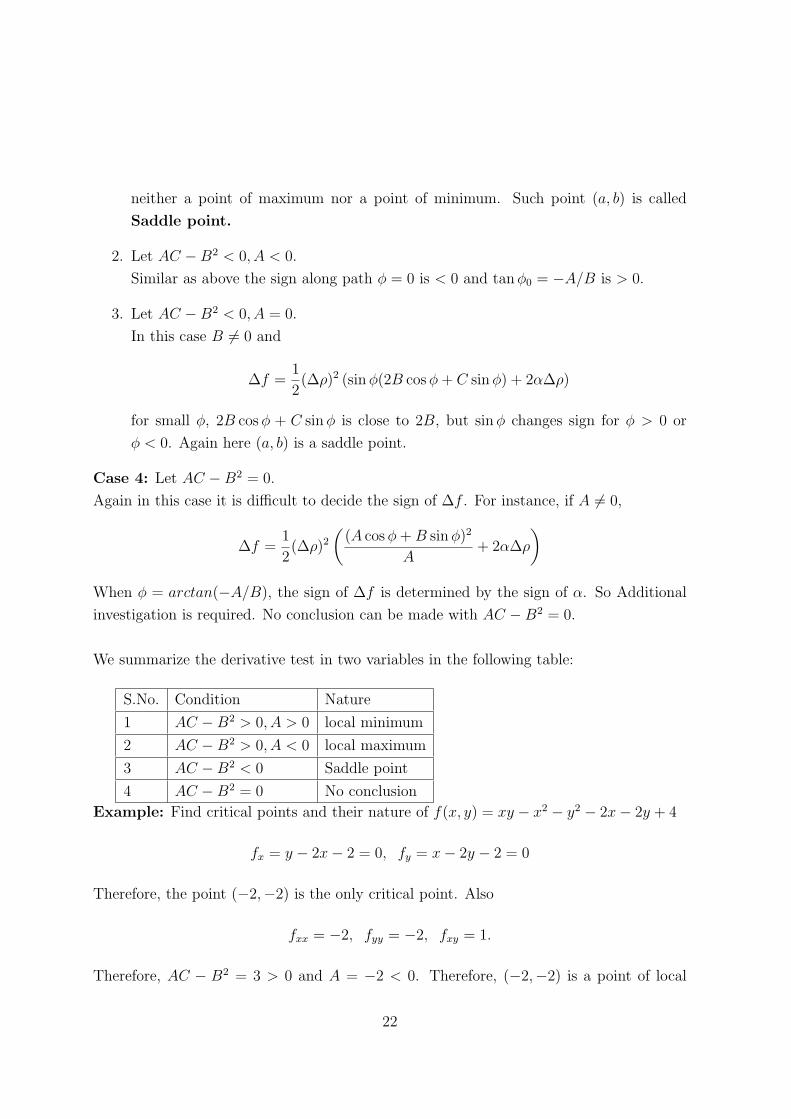
neither a point of maximum nor a point of minimum. Such point (a, b) is called

Saddle point.

2. Let AC − B2 < 0, A < 0.

Similar as above the sign along path φ = 0 is < 0 and tanφ0 = −A/B is > 0.

3. Let AC − B2 < 0, A = 0.

In this case B = 0 and

Δf =1

2(Δρ)2 (sinφ(2B cosφ+ C sinφ) + 2αΔρ)

for small φ, 2B cosφ + C sinφ is close to 2B, but sinφ changes sign for φ > 0 or

φ < 0. Again here (a, b) is a saddle point.

Case 4: Let AC − B2 = 0.

Again in this case it is difficult to decide the sign of Δf . For instance, if A = 0,

Δf =1

2(Δρ)2

((A cosφ+B sinφ)2

A+ 2αΔρ

)

When φ = arctan(−A/B), the sign of Δf is determined by the sign of α. So Additional

investigation is required. No conclusion can be made with AC − B2 = 0.

We summarize the derivative test in two variables in the following table:

S.No. Condition Nature

1 AC − B2 > 0, A > 0 local minimum

2 AC − B2 > 0, A < 0 local maximum

3 AC − B2 < 0 Saddle point

4 AC − B2 = 0 No conclusion

Example: Find critical points and their nature of f(x, y) = xy − x2 − y2 − 2x− 2y + 4

fx = y − 2x− 2 = 0, fy = x− 2y − 2 = 0

Therefore, the point (−2,−2) is the only critical point. Also

fxx = −2, fyy = −2, fxy = 1.

Therefore, AC − B2 = 3 > 0 and A = −2 < 0. Therefore, (−2,−2) is a point of local

22

Figure 15:

maximum.

The following is an example where the derivative test fails.

Example: Consider the function f(x, y) = (x − y)2, then fx = 0, fy = 0 implies x = y.

Also, AC − B2 = 0. Moreover, all third order partial derivatives are zero. so no further

information can be expected from Taylor’s theorem.

Global/Absolute maxima and Minima on closed and bounded domains:

1. Find all critical points of f(x, y). These are the interior points where partial deriva-

tives can be defined.

2. Restrict the function to the each piece of the boundary. This will be one variable

function defined on closed interval I(say) and use the derivative test of one variable

calculus to find the critical points that lie in the open interval and their nature.

3. Find the end points of these intervals I and evaluate f(x, y) at these points.

4. The global/Absolute maximum will be the maximum of f among all these points.

5. Similarly for global minimum.

Example: Find the absolute maxima and minima of f(x, y) = 2 + 2x + 2y − x2 − y2 on

the triangular region in the first quadrant bounded by the lines x = 0, y = 0, y = 9− x.

Solution: fx = 2− 2x = 0, fy = 2− 2y = 0 implies that x = 1, y = 1 is the only critical

point and f(1, 1) = 4. fxx = −2, fyy = −2, fxy = 0. Therefore, AC − B2 = 4 > 0 and

A < 0. So this is local maximum.

23

case 1: On the segment y = 0, f(x, y) = f(x, 0) = 2 + 2x − x2 defined on I = [0, 9].

f(0, 0) = 2, f(9, 0) = −61 and the at the interior points where f ′(x, 0) = 2 − 2x = 0. So

x = 1 is the only critical point and f(1, 0) = 3.

case 2: On the segment x = 0, f(0, y) = 2+ 2y− y2 and fy = 2− 2y = 0 implies y = 1

and f(0, 1) = 3.

Case 3: On the segment y = 9− x, we have

f(x, 9− x) = −61 + 18x− 2x2

and the critical point is x = 9/2. At this point f(9/2, 9/2) = −41/2.finally, f(0, 0) = 2, f(9, 0) = f(0, 9) = −61. so the global maximum is 4 at (1, 1) and

minimum is −61 at (9, 0) and (0, 9).

7 Constrained minimization

First, we describe the substitution method. Consider the problem of finding the shortest

distance from origin to the plane z = 2x+ y − 5.

Here we minimize the function f(x, y, z) = x2 + y2 + z2 subject to the constraint 2x+ y−z − 5 = 0. Substituting the constraint in the function, we get

h(x, y) = f(x, y, 2x+ y − 5) = x2 + y2 + (2x+ y − 5)2.

The critical points of this function are

hx = 2x+ 2(2x+ y − 5)(2) = 0, hy = 2y + 2(2x+ y − 5) = 0.

This leads to x = 5/3, y = 5/6. Then z = 2x+ y− 5 implies z = −5/6. We can check that

AC − B2 > 0 and A > 0. So the point (5/3, 5/6,−5/6) is a point of minimum.

Does this substitution method always work? The answer is NO. The following

example explains

Example: The shortest distance from origin to x2 − z2 = 1.

This is minimizing f(x, y, z) = x2 + y2 + z2 subject to the constraint x2 − z2 = 1. Then

substituting z2 = x2 − 1 in f , we get

h(x, y) = f(x, y, x2 − 1) = 2x2 + y2 − 1

24

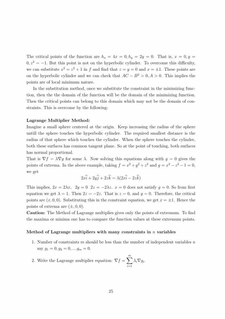
The critical points of the function are hx = 4x = 0, hy = 2y = 0. That is, x = 0, y =

0, z2 = −1. But this point is not on the hyperbolic cylinder. To overcome this difficulty,

we can substitute x2 = z2 + 1 in f and find that z = y = 0 and x = ±1. These points are

on the hyperbolic cylinder and we can check that AC − B2 > 0, A > 0. This implies the

points are of local minimum nature.

In the substitution method, once we substitute the constraint in the minimizing func-

tion, then the the domain of the function will be the domain of the minimizing function.

Then the critical points can belong to this domain which may not be the domain of con-

straints. This is overcome by the following:

Lagrange Multiplier Method:

Imagine a small sphere centered at the origin. Keep increasing the radius of the sphere

untill the sphere touches the hyperbolic cylinder. The required smallest distance is the

radius of that sphere which touches the cylinder. When the sphere touches the cylinder,

both these surfaces has common tangent plane. So at the point of touching, both surfaces

has normal proportional.

That is ∇f = λ∇g for some λ. Now solving this equations along with g = 0 gives the

points of extrema. In the above example, taking f = x2 + y2 + z2 and g = x2− z2− 1 = 0,

we get

2xi+ 2yj + 2zk = λ(2xi− 2zk)

This implies, 2x = 2λx, 2y = 0 2z = −2λz. x = 0 does not satisfy g = 0. So from first

equation we get λ = 1. Then 2z = −2z. That is z = 0, and y = 0. Therefore, the critical

points are (x, 0, 0). Substituting this in the constraint equation, we get x = ±1. Hence thepoints of extrema are (±, 0, 0).Caution: The Method of Lagrange multiplies gives only the points of extremum. To find

the maxima or minima one has to compare the function values at these extremum points.

Method of Lagrange multipliers with many constraints in n variables

1. Number of constraints m should be less than the number of independent variables n

say g1 = 0, g2 = 0, ....gm = 0.

2. Write the Lagrange multiplier equation: ∇f =m∑i=1

λi∇gi.

25

(a) Lagrange multipliers

Figure 16:

3. Solve the set of m+ n equations to find the extremal points

∇f =m∑i=1

λi∇gi, gi = 0, i = 1, 2, ...m

4. Once we have extremum points, compare the values of f at these points to determine

the maxima and minima.

Refereces:

1. Thomas Calculus Chapter 14

2. N. Piskunov, Differential and Integral calculus

26