Sequential Monte Carlo samplers - Oxford Statisticsdoucet/delmoral_doucet... · following two...
26
2006 Royal Statistical Society 1369–7412/06/68411 J. R. Statist. Soc. B (2006) 68, Part 3, pp. 411–436 Sequential Monte Carlo samplers Pierre Del Moral, Universit´ e Nice Sophia Antipolis, France Arnaud Doucet University of British Columbia, Vancouver, Canada and Ajay Jasra University of Cambridge, UK [Received January 2003. Final revision January 2006] Summary. We propose a methodology to sample sequentially from a sequence of probability distributions that are defined on a common space, each distribution being known up to a nor- malizing constant. These probability distributions are approximated by a cloud of weighted ran- dom samples which are propagated over time by using sequential Monte Carlo methods. This methodology allows us to derive simple algorithms to make parallel Markov chain Monte Carlo algorithms interact to perform global optimization and sequential Bayesian estimation and to compute ratios of normalizing constants. We illustrate these algorithms for various integration tasks arising in the context of Bayesian inference. Keywords: Importance sampling; Markov chain Monte Carlo methods; Ratio of normalizing constants; Resampling; Sequential Monte Carlo methods; Simulated annealing 1. Introduction Consider a sequence of probability measures {π n } n∈T that are defined on a common measurable space .E, E /, where T = {1,..., p}. For ease of presentation, we shall assume that each π n .dx/ admits a density π n .x/ with respect to a σ-finite dominating measure denoted dx. We shall refer to n as the time index; this variable is simply a counter and need not have any relationship with ‘real’ time. We also denote, by E n , the support of π n , i.e. E n = {x ∈ E : π n .x/ > 0}. In this paper, we are interested in sampling from the distributions {π n } n∈T sequentially, i.e. first sampling from π 1 , then from π 2 and so on. This problem arises in numerous applications. In the context of sequential Bayesian infer- ence, π n could be the posterior distribution of a parameter given the data collected until time n, e.g. π n .x/ = p.x|y 1 ,..., y n /. In a batch set-up where a fixed set of observations y 1 ,..., y p is available, we could also consider the sequence of distributions p.x|y 1 ,..., y n / for n p for the following two reasons. First, for large data sets, standard simulation methods such as Markov chain Monte Carlo (MCMC) methods require a complete ‘browsing’ of the observations; in contrast, a sequential strategy may have reduced computational complexity. Second, by includ- ing the observations one at a time, the posterior distributions exhibit a beneficial tempering effect (Chopin, 2002). Alternatively, we may want to move from a tractable (easy-to-sample) Address for correspondence: Arnaud Doucet, Department of Statistics and Department of Computer Science, University of British Columbia, 333-6356 Agricultural Road, Vancouver, British Columbia, V6T 1Z2, Canada. E-mail: [email protected]
Transcript of Sequential Monte Carlo samplers - Oxford Statisticsdoucet/delmoral_doucet... · following two...
2006 Royal Statistical Society 1369–7412/06/68411
J. R. Statist. Soc. B (2006)68, Part 3, pp. 411–436
Sequential Monte Carlo samplers
Pierre Del Moral,
Universite Nice Sophia Antipolis, France
Arnaud Doucet
University of British Columbia, Vancouver, Canada
and Ajay Jasra
University of Cambridge, UK
[Received January 2003. Final revision January 2006]
Summary. We propose a methodology to sample sequentially from a sequence of probabilitydistributions that are defined on a common space, each distribution being known up to a nor-malizing constant. These probability distributions are approximated by a cloud of weighted ran-dom samples which are propagated over time by using sequential Monte Carlo methods. Thismethodology allows us to derive simple algorithms to make parallel Markov chain Monte Carloalgorithms interact to perform global optimization and sequential Bayesian estimation and tocompute ratios of normalizing constants. We illustrate these algorithms for various integrationtasks arising in the context of Bayesian inference.
Keywords: Importance sampling; Markov chain Monte Carlo methods; Ratio of normalizingconstants; Resampling; Sequential Monte Carlo methods; Simulated annealing
1. Introduction
Consider a sequence of probability measures {πn}n∈T that are defined on a common measurablespace .E, E/, where T={1, . . . , p}. For ease of presentation, we shall assume that each πn.dx/
admits a density πn.x/ with respect to a σ-finite dominating measure denoted dx. We shall referto n as the time index; this variable is simply a counter and need not have any relationship with‘real’ time. We also denote, by En, the support of πn, i.e. En ={x∈E :πn.x/> 0}. In this paper,we are interested in sampling from the distributions {πn}n∈T sequentially, i.e. first samplingfrom π1, then from π2 and so on.
This problem arises in numerous applications. In the context of sequential Bayesian infer-ence, πn could be the posterior distribution of a parameter given the data collected until timen, e.g. πn.x/=p.x|y1, . . . , yn/. In a batch set-up where a fixed set of observations y1, . . . , yp isavailable, we could also consider the sequence of distributions p.x|y1, . . . , yn/ for n�p for thefollowing two reasons. First, for large data sets, standard simulation methods such as Markovchain Monte Carlo (MCMC) methods require a complete ‘browsing’ of the observations; incontrast, a sequential strategy may have reduced computational complexity. Second, by includ-ing the observations one at a time, the posterior distributions exhibit a beneficial temperingeffect (Chopin, 2002). Alternatively, we may want to move from a tractable (easy-to-sample)
Address for correspondence: Arnaud Doucet, Department of Statistics and Department of Computer Science,University of British Columbia, 333-6356 Agricultural Road, Vancouver, British Columbia, V6T 1Z2, Canada.E-mail: [email protected]
412 P. Del Moral, A. Doucet and A. Jasra
distribution π1 to a distribution of interest, πp, through a sequence of artificial intermediatedistributions (Neal, 2001). In the context of optimization, and in a manner that is similar tosimulated annealing, we could also consider the sequence of distributions πn.x/∝π.x/φn for anincreasing schedule {φn}n∈T.
The tools that are favoured by statisticians, to sample from complex distributions, are MCMCmethods (see, for example, Robert and Casella (2004)). To sample from πn, MCMC meth-ods consist of building an ergodic Markov kernel Kn with invariant distribution πn by usingMetropolis–Hastings (MH) steps and Gibbs moves. MCMC algorithms have been successfullyapplied to many problems in statistics (e.g. mixture modelling (Richardson and Green, 1997)and changepoint analysis (Green, 1995)). However, in general, there are two major drawbackswith MCMC methods. It is difficult to assess when the Markov chain has reached its stationaryregime and it can easily become trapped in local modes. Moreover, MCMC methods cannot beused in a sequential Bayesian estimation context.
In this paper, we propose a different approach to sample from {πn}n∈T that is based onsequential Monte Carlo (SMC) methods (Del Moral, 2004; Doucet et al., 2001; Liu, 2001).Henceforth, the resulting algorithms will be called SMC samplers. More precisely, this is a com-plementary approach to MCMC sampling, as MCMC kernels will often be ingredients of themethods proposed. SMC methods have been recently studied and used extensively in the contextof sequential Bayesian inference. At a given time n, the basic idea is to obtain a large collection ofN weighted random samples {W.i/
n , X.i/n } .i = 1, . . . , N, W.i/
n > 0;ΣNi=1W.i/
n = 1) named particleswhose empirical distribution converges asymptotically (N →∞) to πn, i.e. for any πn-integrablefunction ϕ : E→R
N∑i=1
W.i/n ϕ.X.i/
n /→Eπn.ϕ/ almost surely
where
Eπn.ϕ/=∫
E
ϕ.x/πn.x/dx: .1/
These particles are carried forward over time by using a combination of sequential importancesampling (IS) and resampling ideas.
Standard SMC algorithms in the literature do not apply to the problems that were describedabove. This is because these algorithms deal with the case where the target distribution of inter-est, at time n, is defined on Sn with dim.Sn−1/ < dim.Sn/, e.g. Sn = En. Conversely, we areinterested in the case where the distributions {πn}n∈T are all defined on a common space E.Our approach has some connections with adaptive IS methods (West, 1993; Oh and Berger,1993; Givens and Raftery, 1996), resample–move (RM) strategies (Chopin, 2002; Gilks andBerzuini, 2001), Annealed IS (AIS) (Neal, 2001) and population Monte Carlo methods (Cappeet al., 2004) which are detailed in Section 3. However, the generic framework that we presenthere is more flexible. It allows us to define general moves and can be used in scenarios wherepreviously developed methodologies do not apply (see Section 5). Additionally, we can developnew algorithms to make parallel MCMC runs interact in a simple way, to perform global opti-mization or to solve sequential Bayesian estimation problems. It is also possible to estimateratios of normalizing constants as a by-product of the algorithm. As for MCMC sampling, theperformance of these algorithms is highly dependent on the target distributions {πn}n∈T andproposal distributions that are used to explore the space.
This paper focuses on the algorithmic aspects of SMC samplers. However, it is worth notingthat our algorithms can be interpreted as interacting particle approximations of a Feynman–Kac
Monte Carlo Samplers 413
flow in distribution space. Many general convergence results are available for these approxima-tions and, consequently, for SMC samplers (Del Moral, 2004). Nevertheless, the SMC samplersthat are developed here are such that many known estimates on the asymptotic behaviour ofthese general processes can be greatly improved. Several of these results can be found in DelMoral and Doucet (2003). In this paper we provide the expressions for the asymptotic variancesthat are associated with central limit theorems.
The rest of the paper is organized as follows. In Section 2, we present a generic sequential IS(SIS) algorithm to sample from a sequence of distributions {πn}n∈T. We outline the limitationsof this approach which severely restricts the way that we can move the particles around the space.In Section 3, we provide a method to circumvent this problem by building an artificial sequenceof joint distributions which admits fixed marginals. We provide guidelines for the design ofefficient algorithms. Some extensions and connections with previous work are outlined. Theremaining sections describe how to apply the SMC sampler methodology to two importantspecial cases. Section 4 presents a generic approach to convert an MCMC sampler into an SMCsampler to sample from a fixed target distribution. This is illustrated on a Bayesian analysis offinite mixture distributions. Finally, Section 5 presents an application of SMC samplers to asequential, transdimensional Bayesian inference problem. The proofs of the results in Section 3can be found in Appendix A.
2. Sequential importance sampling
In this section, we describe a generic iterative SIS method to sample from a sequence of distri-butions {πn}n∈T. We provide a review of the standard IS method; then we outline its limitationsand describe a sequential version of the algorithm.
2.1. Importance samplingLet πn be a target density on E such that
πn.x/=γn.x/=Zn
where γn : E→R+ is known pointwise and the normalizing constant Zn is unknown. Let ηn.x/
be a positive density with respect to dx, referred to as the importance distribution. IS is basedon the identities
Eπn.ϕ/=Z−1n
∫E
ϕ.x/wn.x/ηn.x/dx, .2/
Zn =∫
E
wn.x/ηn.x/dx, .3/
where the unnormalized importance weight function is equal to
wn.x/=γn.x/=ηn.x/: .4/
By sampling N particles {X.i/n } from ηn and substituting the Monte Carlo approximation
ηNn .dx/= 1
N
N∑i=1
δX
.i/n
.dx/
(with δ denoting Dirac measure) of this distribution into equations (2) and (3), we obtain anapproximation for Eπn.ϕ/ and Zn.

414 P. Del Moral, A. Doucet and A. Jasra
In statistics applications, we are typically interested in estimating equation (1) for a largerange of test functions ϕ. In these cases, we are usually trying to select ηn ‘close’ to πn as thevariance is approximately proportional to 1 + varηn{wn.Xn/} (see Liu (2001), pages 35–36).Unfortunately, selecting such an importance distribution is very difficult when πn is a non-standard high dimensional distribution. As a result, despite its relative simplicity, IS is almostnever used when MCMC methods can be applied.
2.2. Sequential importance samplingTo obtain better importance distributions, we propose the following sequential method. At timen = 1, we start with a target distribution π1 which is assumed to be easy to approximate effi-ciently by using IS, i.e. η1 can be selected such that the variance of the importance weights (4) issmall. In the simplest case, η1 =π1. Then, at time n=2, we consider the new target distributionπ2. To build the associated IS distribution η2, we use the particles sampled at time n = 1, say{X
.i/1 }. The rationale is that, if π1 and π2 are not too different from one another, then it should
be possible to move the particles {X.i/1 } in the regions of high probability density of π2 in a
sensible way.At time n−1 we have N particles {X
.i/n−1} distributed according to ηn−1. We propose to move
these particles by using a Markov kernel Kn : E × E → [0, 1], with associated density denotedKn.x, x′/. The particles {X.i/
n } that are obtained this way are marginally distributed accordingto
ηn.x′/=∫
E
ηn−1.x/Kn.x, x′/dx: .5/
If ηn can be computed pointwise, then it is possible to use the standard IS estimates of πn andZn.
2.3. Algorithm settingsThis SIS strategy is very general. There are many potential choices for {πn}n∈T leading to vari-ous integration and optimization algorithms.
2.3.1. Sequence of distributions {πn}
(a) In the context of Bayesian inference for static parameters, where p observations .y1, . . . ,yp/ are available, we can consider
πn.x/=p.x|y1, . . . , yn/: .6/
See Chopin (2002) for such applications.(b) It can be of interest to consider an inhomogeneous sequence of distributions to move
‘smoothly’ from a tractable distribution π1 = µ1 to a target distribution π through asequence of intermediate distributions. For example, we could select a geometric path(Gelman and Meng, 1998; Neal, 2001)
πn.x/∝π.x/φnµ1.x/1−φn .7/
with 0�φ1 < . . . <φp =1.Alternatively, we could simply consider the case where πn =π for all n ∈ T. This has
been proposed numerous times in the literature. However, if π is a complex distribution,it is difficult to build a sensible initial importance distribution. In particular, such algo-

Monte Carlo Samplers 415
rithms may fail when the target is multimodal with well-separated narrow modes. Indeed,in this case, the probability of obtaining samples in all the modes of the target is verysmall and an importance distribution that is based on these initial particles is likely tobe inefficient. Therefore, for difficult scenarios, it is unlikely that such approaches will berobust.
(c) For global optimization, as in simulated annealing, we can select
πn.x/∝π.x/φn .8/
where {φn}n∈T is an increasing sequence such that φp →∞ for large p.(d) Assume that we are interested in estimating the probability of a rare event, A∈E , under
a probability measure π (π.A/≈ 0). In most of these applications, π is typically easy tosample from and the normalizing constant of its density is known. We can consider thesequence of distributions
πn.x/∝π.x/ IEn.x/
where En ∈E ∀n∈T, IA.x/ is the indicator function for A∈E and E1 ⊃E2 ⊃ . . .⊃Ep−1 ⊃Ep, E1 =E and Ep =A. An estimate of π.A/ is given by an estimate of the normalizingconstant Zp:
2.3.2. Sequence of transition kernels {Kn}It is easily seen that the optimal proposal, in the sense of minimizing the variance of the impor-tance weights, is Kn.x, x′/ = πn.x′/. As this choice is impossible, we must formulate sensiblealternatives.
2.3.2.1. Independent proposals. It is possible to select Kn.x, x′/ = Kn.x′/ where Kn.·/ is astandard distribution (e.g. Gaussian or multinomial) whose parameters can be determined byusing some statistics based on ηN
n−1. This approach is standard in the literature, e.g. West (1993).However, independent proposals appear overly restrictive and it seems sensible to design localmoves in high dimensional spaces.
2.3.2.2. Local random-walk moves. A standard alternative consists of using for Kn.x, x′/ arandom-walk kernel. This idea has appeared several times in the literature where Kn.x, x′/ isselected as a standard smoothing kernel (e.g. Gaussian or Epanechikov), e.g. Givens and Raftery(1996). However, this approach is problematic. Firstly, the choice of the kernel bandwidth isdifficult. Standard rules to determine kernel bandwidths may indeed not be appropriate here,because we are not trying to obtain a kernel density estimate ηN
n−1Kn.x′/ of ηn−1.x′/ but todesign an importance distribution to approximate πn.x′/. Secondly, no information about πn istypically used to build Kn.x, x′/.
Two alternative classes of local moves exploiting the structure of πn are now proposed.
2.3.2.3. Markov chain Monte Carlo moves. It is natural to set Kn as an MCMC kernel ofinvariant distribution πn. In particular, this approach is justified if either Kn is fast mixing and/orπn is slowly evolving so that we can expect ηn to be reasonably close to the target distribution.In this case, the resulting algorithm is an IS technique which would allow us to correct for thefact that the N inhomogeneous Markov chains {X.i/
n } are such that ηn =πn. This is an attractive
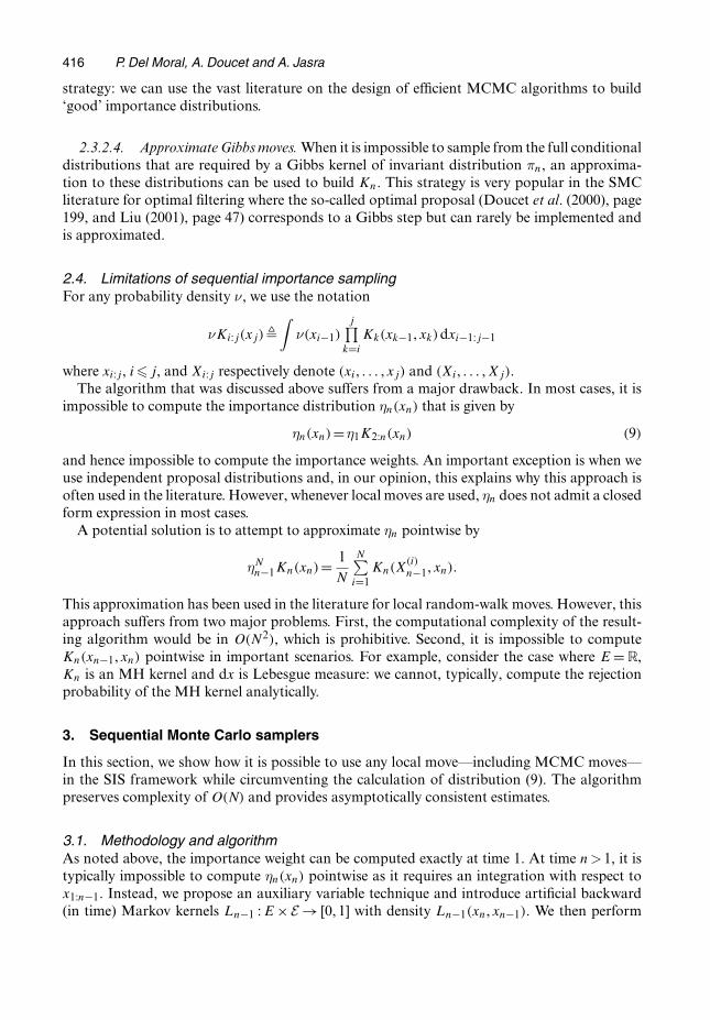
416 P. Del Moral, A. Doucet and A. Jasra
strategy: we can use the vast literature on the design of efficient MCMC algorithms to build‘good’ importance distributions.
2.3.2.4. Approximate Gibbs moves. When it is impossible to sample from the full conditionaldistributions that are required by a Gibbs kernel of invariant distribution πn, an approxima-tion to these distributions can be used to build Kn. This strategy is very popular in the SMCliterature for optimal filtering where the so-called optimal proposal (Doucet et al. (2000), page199, and Liu (2001), page 47) corresponds to a Gibbs step but can rarely be implemented andis approximated.
2.4. Limitations of sequential importance samplingFor any probability density ν, we use the notation
νKi:j.xj/�∫
ν.xi−1/j∏
k=i
Kk.xk−1, xk/dxi−1:j−1
where xi:j, i� j, and Xi:j respectively denote .xi, . . . , xj/ and .Xi, . . . , Xj/.The algorithm that was discussed above suffers from a major drawback. In most cases, it is
impossible to compute the importance distribution ηn.xn/ that is given by
ηn.xn/=η1K2:n.xn/ .9/
and hence impossible to compute the importance weights. An important exception is when weuse independent proposal distributions and, in our opinion, this explains why this approach isoften used in the literature. However, whenever local moves are used, ηn does not admit a closedform expression in most cases.
A potential solution is to attempt to approximate ηn pointwise by
ηNn−1Kn.xn/= 1
N
N∑i=1
Kn.X.i/n−1, xn/:
This approximation has been used in the literature for local random-walk moves. However, thisapproach suffers from two major problems. First, the computational complexity of the result-ing algorithm would be in O.N2/, which is prohibitive. Second, it is impossible to computeKn.xn−1, xn/ pointwise in important scenarios. For example, consider the case where E = R,Kn is an MH kernel and dx is Lebesgue measure: we cannot, typically, compute the rejectionprobability of the MH kernel analytically.
3. Sequential Monte Carlo samplers
In this section, we show how it is possible to use any local move—including MCMC moves—in the SIS framework while circumventing the calculation of distribution (9). The algorithmpreserves complexity of O.N/ and provides asymptotically consistent estimates.
3.1. Methodology and algorithmAs noted above, the importance weight can be computed exactly at time 1. At time n > 1, it istypically impossible to compute ηn.xn/ pointwise as it requires an integration with respect tox1:n−1. Instead, we propose an auxiliary variable technique and introduce artificial backward(in time) Markov kernels Ln−1 : E × E → [0, 1] with density Ln−1.xn, xn−1/. We then perform

Monte Carlo Samplers 417
IS between the joint importance distribution ηn.x1:n/ and the artificial joint target distributiondefined by
πn.x1:n/= γn.x1:n/=Zn
where
γn.x1:n/=γn.xn/n−1∏k=1
Lk.xk+1, xk/:
As πn.x1:n/ admits πn.xn/ as a marginal by construction, IS provides an estimate of this distribu-tion and its normalizing constant. By proceeding thus, we have defined a sequence of probabilitydistributions {πn} whose dimension is increasing over time; i.e. πn is defined on En. We are thenback to the ‘standard’ SMC framework that was described, for example, in Del Moral (2004),Doucet et al. (2001) and Liu (2001). We now describe a generic SMC algorithm to samplefrom this sequence of distributions based on SIS resampling methodology.
At time n−1, assume that a set of weighted particles {W.i/n−1, X
.i/1:n−1} .i=1, . . . , N/ approxi-
mating πn−1 is available,
πNn−1.dx1:n−1/=
N∑i=1
W.i/n−1δX
.i/1:n−1
.dx1:n−1/, .10/
W.i/n−1 =wn−1.X
.i/1:n−1/
/N∑
j=1wn−1.X
.j/1:n−1/:
At time n, we extend the path of each particle with a Markov kernel Kn.xn−1, xn/. IS is thenused to correct for the discrepancy between the sampling distribution ηn.x1:n/ and πn.x1:n/. Inthis case the new expression for the unnormalized importance weights is given by
wn.x1:n/= γn.x1:n/=ηn.x1:n/ .11/
=wn−1.x1:n−1/ wn.xn−1, xn/
where the so-called (unnormalized) incremental weight wn.xn−1, xn/ is equal to
wn.xn−1, xn/= γn.xn/Ln−1.xn, xn−1/
γn−1.xn−1/Kn.xn−1, xn/: .12/
As the discrepancy between ηn and πn tends to increase with n, the variance of the unnormal-ized importance weights tends to increase, resulting in a potential degeneracy of the particleapproximation. This degeneracy is routinely measured by using the effective sample size (ESS)criterion {ΣN
i=1.W.i/n /2}−1 (Liu and Chen, 1998). The ESS takes values between 1 and N. If the
degeneracy is too high, i.e. the ESS is below a prespecified threshold, say N=2, then each par-ticle X
.i/1:n is copied N.i/
n times under the constraint ΣNi=1N.i/
n =N, the expectation of N.i/n being
equal to NW.i/n such that particles with high weights are copied multiple times whereas particles
with low weights are discarded. Finally, all resampled particles are assigned equal weights. Thesimplest way to perform resampling consists of sampling the N new particles from the weighteddistribution πN
n ; the resulting {N.i/n } are distributed according to a multinomial distribution of
parameters {W.i/n }. Stratified resampling (Kitagawa, 1996) and residual resampling can also be
used and all of these reduce the variance of N.i/n relatively to that of the multinomial scheme.
A summary of the algorithm is described in the next subsection. The complexity of thisalgorithm is in O.N/ and it can be parallelized easily.

418 P. Del Moral, A. Doucet and A. Jasra
3.1.1. Algorithm: sequential Monte Carlo sampler
Step 1: initialization—set n=1;for i=1, . . . , N draw X
.i/1 ∼η1;
evaluate {w1.X.i/1 /} by using equation (4) and normalize these weights to obtain {W
.i/1 }.
Iterate steps 2 and 3.Step 2: resampling—
if ESS <T (for some threshold T ), resample the particles and set W.i/n =1=N.
Step 3: sampling—set n=n+1; if n=p+1 stop;for i=1, . . . , N draw X.i/
n ∼Kn.X.i/n−1, ·/;
evaluate {wn.X.i/n−1:n/} by using equation (12) and normalize the weights
W.i/n =W
.i/n−1 wn.X
.i/n−1:n/
/ N∑j=1
W.j/n−1 wn.X
.j/n−1:n/:
Remark 1. If the weights {W.i/n } are independent of {X.i/
n }, then the particles {X.i/n } should
be sampled after the weights {W.i/n } have been computed and after the particle approximation
{W.i/n , X
.i/n−1} of πn.xn−1/ has possibly been resampled. This scenario appears when {Ln} is given
by equation (30) in Section 3.3.2.3.
Remark 2. It is also possible to derive an auxiliary version of algorithm 1 in the spirit of Pittand Shephard (1999).
3.2. Notes on algorithm3.2.1. Estimates of target distributions and normalizing constantsAt time n, we obtain after the sampling step a particle approximation {W.i/
n , X.i/1:n} of πn.x1:n/.
As the target πn.xn/ is a marginal of πn.x1:n/ by construction, an approximation of it is givenby
πNn .dx/=
N∑i=1
W.i/n δ
X.i/n
.dx/: .13/
The particle approximation {W.i/n−1, X
.i/n−1:n} of πn−1.xn−1/Kn.xn−1, xn/ that is obtained after
the sampling step also allows us to approximate
Zn
Zn−1=
∫γn.xn/dxn∫
γn−1.xn−1/ dxn−1
by
Zn
Zn−1=
N∑i=1
W.i/n−1wn.X
.i/n−1:n/: .14/
To estimate Zn=Z1, we can use the product of estimates of the form (14) from time k = 2 tok =n. However, if we do not resample at each iteration, a simpler alternative is given by

Monte Carlo Samplers 419
Zn
Z1=
rn−1+1∏j=1
Zkj
Zkj−1
,
with
Zkj
Zkj−1
=N∑
i=1W
.i/kj−1
kj∏m=kj−1+1
wm.X.i/m−1:m/ .15/
where k0 =1, kj is the jth time index at which we resample for j> 1. The number of resamplingsteps between 1 and n−1 is denoted rn−1 and we set krn−1+1 =n.
There is a potential alternative estimate for ratios of normalizing constants that is based onpath sampling (Gelman and Meng, 1998). Indeed, consider a continuous path of distributions
πθ.t/ =γθ.t/=Zθ.t/
where t ∈ [0, 1], θ.0/ = 0 and θ.1/ = 1. Then, under regularity assumptions, we have the pathsampling identity
log(Z1
Z0
)=
∫ 1
0
dθ.t/
dt
∫d[log{γθ.t/.x/}]
dtπθ.t/.dx/dt:
In the SMC samplers context, if we consider a sequence of p + 1 intermediate distributionsdenoted here πθ.k=P/, k=0, . . . , p, to move from π0 to π1 then the above equation can be approxi-mated by using a trapezoidal integration scheme and substituting πN
θ.k=P/.dx/ for πθ.k=P/.dx/.Some applications of this identity in an SMC framework are detailed in Johansen et al. (2005)and Rousset and Stoltz (2005).
3.2.2. Mixture of Markov kernelsThe algorithm that is described in this section must be interpreted as the basic element of morecomplex algorithms. It is to SMC sampling what the MH algorithm is to MCMC sampling. Forcomplex MCMC problems, one typically uses a combination of MH steps where the J compo-nents of x say .x1, . . . , xJ / are updated in subblocks. Similarly, to sample from high dimensionaldistributions, a practical SMC sampler can update the components of x via subblocks and amixture of transition kernels can be used at each time n.
Let us assume that Kn.xn−1, xn/ is of the form
Kn.xn−1, xn/=M∑
m=1αn,m.xn−1/Kn,m.xn−1, xn/ .16/
where αn,m.xn−1/� 0, ΣMm=1αn,m.xn−1/= 1 and {Kn,m} is a collection of transition kernels. In
this case, the incremental weights can be computed by the standard formula (12). However, thiscould be too expensive if M is large. An alternative, valid, approach consists of considering abackward Markov kernel of the form
Ln−1.xn, xn−1/=M∑
m=1βn−1,m.xn/Ln−1,m.xn, xn−1/ .17/
where βn−1,m.xn/ � 0, ΣMm=1βn−1,m.xn/ = 1 and {Ln−1,m} is a collection of backward transi-
tion kernels. We now introduce, explicitly, a discrete latent variable Mn taking values in M={1, . . . , M} such that P.Mn =m/=αn,m.xn−1/ and perform IS on the extended space E×E×M.
420 P. Del Moral, A. Doucet and A. Jasra
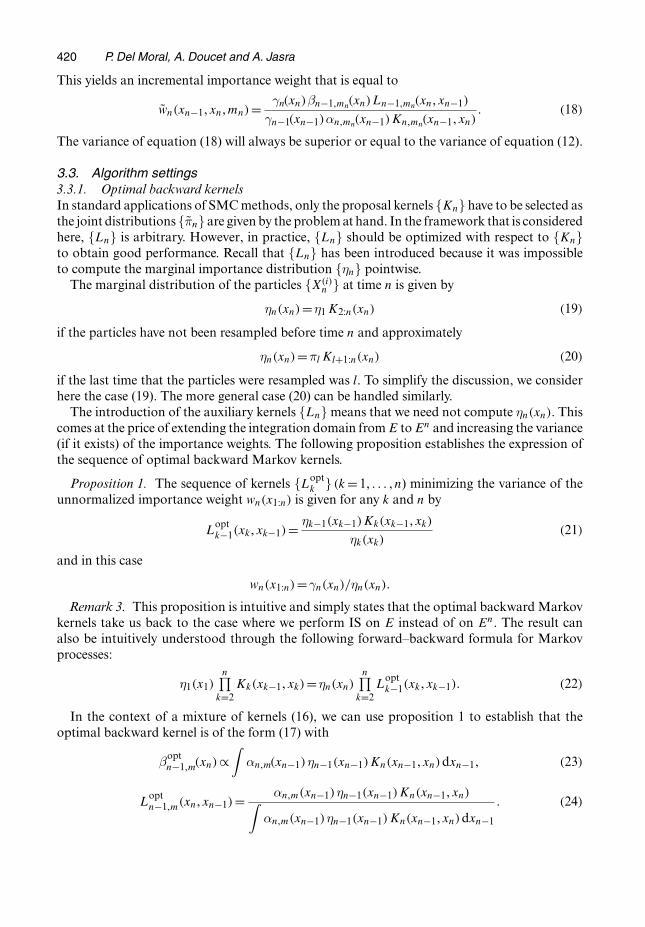
This yields an incremental importance weight that is equal to
wn.xn−1, xn, mn/= γn.xn/βn−1,mn.xn/Ln−1,mn.xn, xn−1/
γn−1.xn−1/αn,mn.xn−1/Kn,mn.xn−1, xn/: .18/
The variance of equation (18) will always be superior or equal to the variance of equation (12).
3.3. Algorithm settings3.3.1. Optimal backward kernelsIn standard applications of SMC methods, only the proposal kernels {Kn} have to be selected asthe joint distributions {πn} are given by the problem at hand. In the framework that is consideredhere, {Ln} is arbitrary. However, in practice, {Ln} should be optimized with respect to {Kn}to obtain good performance. Recall that {Ln} has been introduced because it was impossibleto compute the marginal importance distribution {ηn} pointwise.
The marginal distribution of the particles {X.i/n } at time n is given by
ηn.xn/=η1 K2:n.xn/ .19/
if the particles have not been resampled before time n and approximately
ηn.xn/=πl Kl+1:n.xn/ .20/
if the last time that the particles were resampled was l. To simplify the discussion, we considerhere the case (19). The more general case (20) can be handled similarly.
The introduction of the auxiliary kernels {Ln} means that we need not compute ηn.xn/. Thiscomes at the price of extending the integration domain from E to En and increasing the variance(if it exists) of the importance weights. The following proposition establishes the expression ofthe sequence of optimal backward Markov kernels.
Proposition 1. The sequence of kernels {Loptk } .k = 1, . . . , n) minimizing the variance of the
unnormalized importance weight wn.x1:n/ is given for any k and n by
Loptk−1.xk, xk−1/= ηk−1.xk−1/Kk.xk−1, xk/
ηk.xk/.21/
and in this case
wn.x1:n/=γn.xn/=ηn.xn/:
Remark 3. This proposition is intuitive and simply states that the optimal backward Markovkernels take us back to the case where we perform IS on E instead of on En. The result canalso be intuitively understood through the following forward–backward formula for Markovprocesses:
η1.x1/n∏
k=2Kk.xk−1, xk/=ηn.xn/
n∏k=2
Loptk−1.xk, xk−1/: .22/
In the context of a mixture of kernels (16), we can use proposition 1 to establish that theoptimal backward kernel is of the form (17) with
βoptn−1,m.xn/∝
∫αn,m.xn−1/ηn−1.xn−1/Kn.xn−1, xn/dxn−1, .23/
Loptn−1,m.xn, xn−1/= αn,m.xn−1/ηn−1.xn−1/Kn.xn−1, xn/∫
αn,m.xn−1/ηn−1.xn−1/Kn.xn−1, xn/dxn−1
: .24/

Monte Carlo Samplers 421
3.3.2. Suboptimal backward kernelsIt is typically impossible, in practice, to use the optimal kernels as they themselves rely on mar-ginal distributions which do not admit any closed form expression. However, this suggests thatwe should select {Lk} to approximate equation (21). The key point is that, even if {Lk} is differ-ent from expression (21), the algorithm will still provide asymptotically consistent estimates.Some approximations are now discussed.
3.3.2.1. Substituting πn−1 for ηn−1. One point that is used recurrently is that equation (12)suggests that a sensible, suboptimal, strategy consists of using an Ln which is an approximationof the optimal kernel (21) where we have substituted πn−1 for ηn−1, i.e.
Ln−1.xn, xn−1/= πn−1.xn−1/Kn.xn−1, xn/
πn−1 Kn.xn/.25/
which yields
wn.xn−1, xn/= γn.xn/∫E
γn−1.xn−1/Kn.xn−1, xn/dxn−1
: .26/
It is often more convenient to use equation (26) than equation (21) as {γn} is known analyti-cally, whereas {ηn} is not. If particles have been resampled at time n − 1, then ηn−1 is indeedapproximately equal to πn−1 and thus equation (21) is equal to equation (25).
3.3.2.2. Gibbs-type updates. Consider the case where x= .x1, . . . , xJ / and we only want toupdate the kth (k ∈{1, . . . , J}) component xk of x, denoted xn,k, at time n. It is straightforwardto establish that the proposal distribution minimizing the variance of equation (26) conditionalon xn−1 is a Gibbs update, i.e.
Kn.xn−1, dxn/= δxn−1, −k.dxn,−k/πn.dxn,k|xn,−k/ .27/
where xn,−k = .xn,1, . . . , xn,k−1, xn,k+1, . . . , xn,J /. In this case equations (25) and (26) are givenby
Ln−1.xn, dxn−1/= δxn,−k.dxn−1, −k/πn−1.dxn−1, k|xn−1,−k/,
wn.xn−1, xn/= γn.xn−1, −k, xn,k/
γn−1.xn−1, −k/πn.xn,k|xn−1,−k/:
When it is not possible to sample from πn.xn,k|xn−1, −k/ and/or to compute
γn−1.xn−1,−k/=∫
γn−1.xn−1/dxn−1,k
analytically, this suggests using an approximation πn.xn,k|xn−1,−k/ to πn.xn,k|xn−1,−k/ to sam-ple the particles and another approximation πn−1.xn−1,k|xn−1,−k/ to πn−1.xn−1,k|xn−1,−k/ toobtain
Ln−1.xn, dxn−1/= δxn,−k.dxn−1,−k/ πn−1.dxn−1,k|xn−1,−k/, .28/
wn.xn−1, xn/= γn.xn−1,−k, xn,k/ πn−1.xn−1,k|xn−1,−k/
γn−1.xn−1/ πn.xn,k|xn−1,−k/: .29/

422 P. Del Moral, A. Doucet and A. Jasra
3.3.2.3. Markov chain Monte Carlo kernels. A generic alternative approximation to equa-tion (25) can also be made when Kn is an MCMC kernel of invariant distribution πn. It is givenby
Ln−1.xn, xn−1/= πn.xn−1/Kn.xn−1, xn/
πn.xn/.30/
and will be a good approximation to equation (25) if πn−1 ≈πn; note that equation (30) is thereversed Markov kernel that is associated with Kn: In this case, we have unnormalized incre-mental weight
wn.xn−1, xn/=γn.xn−1/=γn−1.xn−1/: .31/
Contrary to equation (25), this approach does not apply in scenarios where En−1 ⊂ En andEn ∈E ∀n∈T as discussed in Section 5. Indeed, in this case
Ln−1.xn, xn−1/= πn.xn−1/Kn.xn−1, xn/∫En−1
πn.xn−1/Kn.xn−1, xn/dxn−1
.32/
but the denominator of this expression is different from πn.xn/ as the integration is over En−1and not over En.
3.3.2.4. Mixtures of kernels. Practically, we cannot typically compute expressions (23)and (24) in closed form and so approximations are also necessary. As discussed previously, onesuboptimal choice consists of replacing ηn−1 with πn−1 in expressions (23) and (24) or usingfurther approximations like equation (30).
3.3.3. Summarizing remarksTo conclude this subsection, we emphasize that selecting {Ln} as close as possible to {L
optn } is
crucial for this method to be efficient. It could be tempting to select {Ln} in a different way.For example, if we select Ln−1 =Kn then the incremental importance weight looks like an MHratio. However, this ‘aesthetic’ choice will be inefficient in most cases, resulting in importanceweights with a very large or infinite variance.
3.4. Convergence resultsUsing equation (13), the SMC algorithm yields estimates of expectations (1) via
EπNn
.ϕ/=∫
E
ϕ.x/πNn .dx/: .33/
Using equation (14), we can also obtain an estimate of log.Zn=Z1/:
log(
Zn
Z1
)=
n∑k=2
log(
Zk
Zk−1
): .34/
We now present a central limit theorem, giving the asymptotic variance of these estimates in two‘extreme’ cases: when we never resample and when we resample at each iteration. For simplicity,we have considered only the case where multinomial resampling is used (see Chopin (2004a) foranalysis using residual resampling and also Kunsch (2005) for results in the context of filtering).The asymptotic variance expressions (33) and (34) for general SMC algorithms have previously

Monte Carlo Samplers 423
been established in the literature. However, we propose here a new representation which clarifiesthe influence of the kernels {Ln}:
In the following proposition, we denote by N .µ, σ2/ the normal distribution with mean µand variance σ2, convergence in distribution by ‘⇒’,
∫πn.x1:n/dx1:k−1 dxk+1:n by πn.xk/ and∫
πn.x1:n/dx1:k−1 dxk+1:n−1=πn.xk/ by πn.xn|xk/.
Proposition 2. Under the weak integrability conditions that were given in Chopin (2004a),theorem 1, or Del Moral (2004), section 9.4, pages 300–306, we obtain the following results.When no resampling is performed, we have
N1=2{EπNn
.ϕ/−Eπn.ϕ/}⇒N{0, σ2IS,n.ϕ/}
with
σ2IS,n.ϕ/=
∫πn.x1:n/2
ηn.x1:n/{ϕ.xn/−Eπn.ϕ/}2 dx1:n .35/
where the joint importance distribution ηn is given by
ηn.x1:n/=η1.x1/n∏
k=2Kk.xk−1, xk/:
We also have
N1=2{
log(
Zn
Z1
)− log
(Zn
Z1
)}⇒N .0, σ2
IS,n/
with
σ2IS,n =
∫πn.x1:n/2
ηn.x1:n/dx1:n −1: .36/
When multinomial resampling is used at each iteration, we have
N1=2{EπNn.ϕ/−Eπn.ϕ/}⇒N{0, σ2
SMC,n.ϕ/}where, for n�2,
σ2SMC,n.ϕ/=
∫πn.x1/2
η1.x1/
{∫ϕ.xn/ πn.xn|x1/dxn −Eπn.ϕ/
}2
dx1
+n−1∑k=2
∫ {πn.xk/Lk−1.xk, xk−1/}2
πk−1.xk−1/Kk.xk−1, xk/
{∫ϕ.xn/ πn.xn|xk/dxn −Eπn.ϕ/
}2
dxk−1:k
+∫ {πn.xn/Ln−1.xn, xn−1/}2
πn−1.xn−1/Kn.xn−1, xn/{ϕ.xn/−Eπn.ϕ/}2 dxn−1:n .37/
and
N1=2{
log(
Zn
Z1
)− log
(Zn
Z1
)}⇒N .0, σ2
SMC,n/
where
σ2SMC,n =
∫πn.x1/2
η1.x1/dx1 −1+
n−1∑k=2
[∫ {πn.xk/Lk−1.xk, xk−1/}2
πk−1.xk−1/Kk.xk−1, xk/dxk−1:k −1
]
+∫ {πn.xn/Ln−1.xn, xn−1/}2
πn−1.xn−1/Kn.xn−1, xn/dxn−1:n −1: .38/

424 P. Del Moral, A. Doucet and A. Jasra
Remark 4. In the general case, we cannot claim that σ2SMC,n.ϕ/ <σ2
IS,n.ϕ/ or σ2SMC,n <σ2
IS,n.This is because, if the importance weights do not have a large variance, resampling is typicallywasteful as any resampling scheme introduces some variance. However, resampling is beneficialin cases where successive distributions can vary significantly. This has been established theoreti-cally in the filtering case in Chopin (2004a), theorem 5: under mixing assumptions, the varianceis shown to be upper bounded uniformly in time with resampling and to go to ∞ without it.The proof may be adapted to the class of problems that is considered here, and it can be shownthat for expression (8)—under mixing assumptions on {Kn} and using equations (25) or (30) for{Ln}—the variance σ2
SMC,n.ϕ/ is upper bounded uniformly in time for a logarithmic schedule{φn} whereas σ2
IS,n.ϕ/ goes to ∞ with n. Similar results hold for residual resampling. Finally wenote that, although the resampling step appears somewhat artificial in discrete time, it appearsnaturally in the continuous time version of these algorithms (Del Moral, 2004; Rousset andStoltz, 2005).
3.5. Connections with other workTo illustrate the connections with, and differences from, other published work, let us considerthe case where we sample from {πn} using MCMC kernels {Kn} where Kn is πn invariant.
Suppose that, at time n−1, we have the particle approximation {W.i/n−1, X
.i/n−1} of πn−1. Sev-
eral recent algorithms are based on the implicit or explicit use of the backward kernel (30). Inthe case that is addressed here, where all the target distributions are defined on the same space,it was used for example in Chopin (2002), Jarzynski (1997) and Neal (2001). In the case wherethe dimension of the target distributions increases over time, it was used in Gilks and Berzuini(2001) and MacEachern et al. (1999).
For the algorithms that are listed above, the associated backward kernels lead to the incre-mental weights
wn.X.i/n−1, X.i/
n /∝πn.X.i/n−1/=πn−1.X
.i/n−1/: .39/
The potential problem with expression (39) is that these weights are independent of {X.i/n }
where X.i/n ∼ Kn.X
.i/n−1, ·/. In particular, the variance of expression (39) will typically be high
if the discrepancy between πn−1 and πn is large even if the kernel Kn mixes very well. Thisresult is counter-intuitive. In the context of AIS (Neal, 2001) where the sequence of p targetdistributions (7) is supposed to satisfy πn−1 ≈ πn, this is not a problem. However, if succes-sive distributions vary significantly, as in sequential Bayesian estimation, this can become asignificant problem. For example, in the limiting case where Kn.xn−1, xn/ =πn.xn/, we wouldend up with a particle approximation {W.i/
n , X.i/n } of πn where the weights {W.i/
n } have a highvariance whereas {X.i/
n } are independent and identically distributed samples from πn; this isclearly suboptimal.
To deal with this problem, RM strategies were used by (among others) Chopin (2002) andGilks and Berzuini (2001). RM corresponds to the SMC algorithm that is described in Sec-tion 3 using the backward kernel (30). RM resamples the particle approximation {W.i/
n , X.i/n−1}
of πn.xn−1/ if the variance (that is measured approximately through the ESS) is high and onlythen do we sample {X.i/
n } to obtain a particle approximation {N−1, X.i/n } of πn, i.e. all parti-
cles have an equal weight. This can be expected to improve over not resampling if consecutivetargets differ significantly and the kernels {Kn} mix reasonably well; we demonstrate this inSection 4.
Proposition 1 suggests that a better choice (than equation (30)) of backward kernels is givenby equation (25) for which the incremental weights are given by

Monte Carlo Samplers 425
wn.X.i/n−1, X.i/
n /∝ πn.X.i/n /
πn−1Kn.X.i/n /
: .40/
Expression (40) is much more intuitive than expression (39). It depends on Kn and thus theexpression of the weights (40) reflects the mixing properties of the kernel Kn. In particular, thevariance of expression (40) decreases as the mixing properties of the kernel increases.
To illustrate the difference between SMC sampling using expression (40) instead of expres-sion (39), consider the case where x = .x1, . . . , xJ / and we use the Gibbs kernel (27) to updatethe component xk so that expression (40) is given by
wn.X.i/n−1, X.i/
n /∝πn.X.i/n−1,−k/=πn−1.X
.i/n−1,−k/: .41/
By a simple Rao–Blackwell argument, the variance of expression (41) is always smaller than thevariance of expression (39). The difference will be particularly significant in scenarios where themarginals πn−1.x−k/ and πn.x−k/ are close to each other but the full conditional distributionsπn.xk|x−k/ and πn−1.xk|x−k/ differ significantly. In such cases, SMC sampling using expres-sion (39) resamples many more times than SMC sampling using expression (41). Such scenariosappear for example in sequential Bayesian inference as described in Section 5 where each newobservation only modifies the distribution of a subset of the variables significantly.
It is, unfortunately, not always possible to use equation (25) instead of equation (30) as anintegral appears in expression (40). However, if the full conditional distributions of πn−1 andπn can be approximated analytically, it is possible to use equations (28) and (29) instead.
Recent work of Cappe et al. (2004) is another special case of the framework proposed. Theyconsidered the homogeneous case where πn = π and Ln.x, x′/ = π.x′/. Their algorithm cor-responds to the case where Kn.x, x′/=Kn.x′/ and the parameters of Kn.x′/ are determined byusing statistics over the entire population of particles at time n−1. Extensions of this work formissing data problems are presented in Celeux et al. (2006).
Finally Liang (2002) presented a related algorithm where πn =π and Kn.x, x′/=Ln.x, x′/=K.x, x′/.
4. From Markov chain Monte Carlo to sequential Monte Carlo samplers
4.1. MethodologyWe now summarize how it is possible to obtain an SMC algorithm to sample from a fixed targetdistribution π, using MCMC kernels or approximate Gibbs steps to move the particles aroundthe space. The procedure is
(a) build a sequence of distributions {πn}, n= 1, . . . , p, such that π1 is easy to sample fromor to approximate and πp =π,
(b) build a sequence of MCMC transition kernels {Kn} such that Kn is πn invariant or Kn isan approximate Gibbs move of invariant distribution πn,
(c) on the basis of {πn} and {Kn}, build a sequence of artificial backward Markov kernels{Ln} approximating {L
optn } (two generic choices are equations (25) and (30); for approxi-
mate Gibbs moves, we can use equation (28)) and(d) use the SMC algorithm that was described in the previous section to approximate {πn}
and to estimate {Zn}.
4.2. Bayesian analysis of finite mixture distributionsIn the following example, we consider a mixture modelling problem. Our objective is to illustratethe potential benefits of resampling in the SMC methodology.

426 P. Del Moral, A. Doucet and A. Jasra
4.2.1. ModelMixture models are typically used to model heterogeneous data, or as a simple means of den-sity estimation; see Richardson and Green (1997) and the references therein for an overview.Bayesian analysis of mixtures has been fairly recent and there is often substantial difficulty insimulation from posterior distributions for such models; see Jasra et al. (2005b) for example.
We use the model of Richardson and Green (1997), which is as follows; data y1, . . . , yc areindependent and identically distributed with distribution
yi|θr ∼r∑
j=1ωj N .µj, λ−1
j /
where θr = .µ1:r, λ1:r, ω1:r/, 2� r<∞ and r known. The parameter space is E=Rr × .R+/r ×Sr
for the r-component mixture model where Sr = {ω1:r : 0 � ωj � 1 ∩ Σrj=1 ωj = 1}. The priors,
which are the same for each component j = 1, . . . , r, are taken to be µj ∼ N .ξ, κ−1/, λj ∼Ga.ν, χ/, ω1:r−1 ∼D.ρ/, where D.ρ/ is the Dirichlet distribution with parameter ρ and Ga.ν, χ/
is the gamma distribution with shape ν and scale χ. We set the priors in an identical manner tothose in Richardson and Green (1997), with the χ-parameter set as the mean of the hyperpriorthat they assigned that parameter.
One particular aspect of this model, which makes it an appropriate test example, is the featureof label switching. As noted above, the priors on each component are exchangeable, and con-sequently, in the posterior, the marginal distribution of µ1 is the same as µ2, i.e. the marginalposterior is equivalent for each component-specific quantity. This provides us with a diagnosticto establish the effectiveness of the simulation procedure. For more discussion see, for example,Jasra et al. (2005b). It should be noted that very long runs of an MCMC sampler targeting πp
could not explore all the modes of this distribution and failed to produce correct estimates (seeJasra et al. (2005b)).
4.2.2. Sequential Monte Carlo samplerWe shall consider AIS and SMC samplers. Both algorithms use the same MCMC kernels Kn
with invariant distribution πn and the same backward kernels (30). The MCMC kernel is acomposition of the following update steps.
(a) Update µ1:r via an MH kernel with an additive normal random-walk proposal.(b) Update λ1:r via an MH kernel with a multiplicative log-normal random-walk proposal.(c) Update ω1:r via an MH kernel with an additive normal random-walk proposal on the
logit scale.
For some of the runs of the algorithm, we shall allow more than one iteration of the aboveMarkov kernel per time step. Finally, the sequence of densities is taken as
πn.θr/∝ l.y1:c; θr/φn f.θr/
where 0�φ1 < . . . <φp =1 are tempering parameters and we have denoted the prior density asf and likelihood function as l.
4.2.3. Illustration4.2.3.1. Data and simulation parameters. For the comparison, we used the simulated data
from Jasra et al. (2005b): 100 simulated data points from an equally weighted mixture of four(i.e. r =4) normal densities with means at (−3,0,3,6) and standard deviations 0.55. We ran SMCsamplers and AIS with MCMC kernels with invariant distribution πn for 50, 100, 200, 500 and
Monte Carlo Samplers 427
1000 time steps with 1 and 10 MCMC iterations per time step. The proposal variances for theMH steps were the same for both procedures and were dynamically falling to produce an aver-age acceptance rate in .0:15, 0:6/. The initial importance distribution was the prior. The C++code and the data are available at http://www.cs.ubc.ca/∼arnaud/smcsamplers.html.
We ran the SMC algorithm with N =1000 particles and we ran AIS for a similar central pro-cessor unit time. The absence of a resampling step allows AIS to run for a few more iterationsthan SMC sampling. We ran each sampler 10 times (i.e. for each time specification and itera-tion number, each time with 1000 particles). For this demonstration, the resampling thresholdwas 500 particles. We use systematic resampling. The results with residual resampling are verysimilar.
We selected a piecewise linear cooling schedule {φn}. Over 1000 time steps, the sequenceincreased uniformly from 0 to 15=100 for the first 200 time points, then from 15=100 to 40=100for the next 400 and finally from 40=100 to 1 for the last 400 time points. The other time spec-ifications had the same proportion of time attributed to the tempering parameter setting. Thechoice was made to allow an initially slow evolution of the densities and then to allow morecomplex densities to appear at a faster rate. We note that other cooling schedules may be imple-mented (such as logarithmic or quadratic) but we did not find significant improvement withsuch approaches.
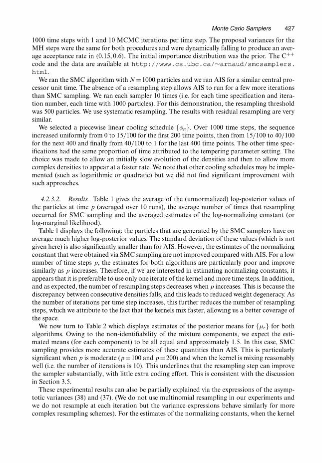
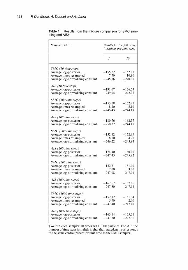
4.2.3.2. Results. Table 1 gives the average of the (unnormalized) log-posterior values ofthe particles at time p (averaged over 10 runs), the average number of times that resamplingoccurred for SMC sampling and the averaged estimates of the log-normalizing constant (orlog-marginal likelihood).
Table 1 displays the following: the particles that are generated by the SMC samplers have onaverage much higher log-posterior values. The standard deviation of these values (which is notgiven here) is also significantly smaller than for AIS. However, the estimates of the normalizingconstant that were obtained via SMC sampling are not improved compared with AIS. For a lownumber of time steps p, the estimates for both algorithms are particularly poor and improvesimilarly as p increases. Therefore, if we are interested in estimating normalizing constants, itappears that it is preferable to use only one iterate of the kernel and more time steps. In addition,and as expected, the number of resampling steps decreases when p increases. This is because thediscrepancy between consecutive densities falls, and this leads to reduced weight degeneracy. Asthe number of iterations per time step increases, this further reduces the number of resamplingsteps, which we attribute to the fact that the kernels mix faster, allowing us a better coverage ofthe space.
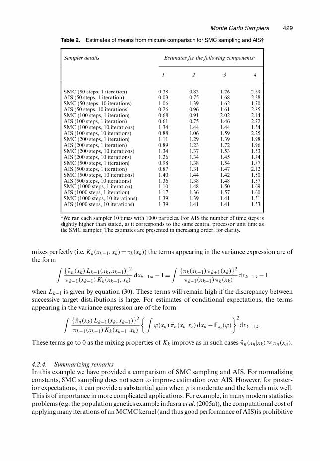
We now turn to Table 2 which displays estimates of the posterior means for {µr} for bothalgorithms. Owing to the non-identifiability of the mixture components, we expect the esti-mated means (for each component) to be all equal and approximately 1.5. In this case, SMCsampling provides more accurate estimates of these quantities than AIS. This is particularlysignificant when p is moderate (p=100 and p=200/ and when the kernel is mixing reasonablywell (i.e. the number of iterations is 10). This underlines that the resampling step can improvethe sampler substantially, with little extra coding effort. This is consistent with the discussionin Section 3.5.
These experimental results can also be partially explained via the expressions of the asymp-totic variances (38) and (37). (We do not use multinomial resampling in our experiments andwe do not resample at each iteration but the variance expressions behave similarly for morecomplex resampling schemes). For the estimates of the normalizing constants, when the kernel
428 P. Del Moral, A. Doucet and A. Jasra
Table 1. Results from the mixture comparison for SMC sam-pling and AIS†
Sampler details Results for the followingiterations per time step:
1 10
SMC (50 time steps)Average log-posterior −155.22 −152.03Average times resampled 7.70 10.90Average log-normalizing constant −245.86 −240.90
AIS (50 time steps)Average log-posterior −191.07 −166.73Average log-normalizing constant −249.04 −242.07
SMC (100 time steps)Average log-posterior −153.08 −152.97Average times resampled 8.20 5.10Average log-normalizing constant −245.43 −244.18
AIS (100 time steps)Average log-posterior −180.76 −162.37Average log-normalizing constant −250.22 −244.17
SMC (200 time steps)Average log-posterior −152.62 −152.99Average times resampled 8.30 4.20Average log-normalizing constant −246.22 −245.84
AIS (200 time steps)Average log-posterior −174.40 −160.00Average log-normalizing constant −247.45 −245.92
SMC (500 time steps)Average log-posterior −152.31 −151.90Average times resampled 7.00 3.00Average log-normalizing constant −247.08 −247.01
AIS (500 time steps)Average log-posterior −167.67 −157.06Average log-normalizing constant −247.30 −247.94
SMC (1000 time steps)Average log-posterior −152.12 −151.94Average times resampled 5.70 2.00Average log-normalizing constant −247.40 −247.40
AIS (1000 time steps)Average log-posterior −163.14 −155.31Average log-normalizing constant −247.50 −247.36
†We ran each sampler 10 times with 1000 particles. For AIS thenumber of time steps is slightly higher than stated, as it correspondsto the same central processor unit time as the SMC sampler.
Monte Carlo Samplers 429
Table 2. Estimates of means from mixture comparison for SMC sampling and AIS†
Sampler details Estimates for the following components:
1 2 3 4
SMC (50 steps, 1 iteration) 0.38 0.83 1.76 2.69AIS (50 steps, 1 iteration) 0.03 0.75 1.68 2.28SMC (50 steps, 10 iterations) 1.06 1.39 1.62 1.70AIS (50 steps, 10 iterations) 0.26 0.96 1.61 2.85SMC (100 steps, 1 iteration) 0.68 0.91 2.02 2.14AIS (100 steps, 1 iteration) 0.61 0.75 1.46 2.72SMC (100 steps, 10 iterations) 1.34 1.44 1.44 1.54AIS (100 steps, 10 iterations) 0.88 1.06 1.59 2.25SMC (200 steps, 1 iteration) 1.11 1.29 1.39 1.98AIS (200 steps, 1 iteration) 0.89 1.23 1.72 1.96SMC (200 steps, 10 iterations) 1.34 1.37 1.53 1.53AIS (200 steps, 10 iterations) 1.26 1.34 1.45 1.74SMC (500 steps, 1 iteration) 0.98 1.38 1.54 1.87AIS (500 steps, 1 iteration) 0.87 1.31 1.47 2.12SMC (500 steps, 10 iterations) 1.40 1.44 1.42 1.50AIS (500 steps, 10 iterations) 1.36 1.38 1.48 1.57SMC (1000 steps, 1 iteration) 1.10 1.48 1.50 1.69AIS (1000 steps, 1 iteration) 1.17 1.36 1.57 1.60SMC (1000 steps, 10 iterations) 1.39 1.39 1.41 1.51AIS (1000 steps, 10 iterations) 1.39 1.41 1.41 1.53
†We ran each sampler 10 times with 1000 particles. For AIS the number of time steps isslightly higher than stated, as it corresponds to the same central processor unit time asthe SMC sampler. The estimates are presented in increasing order, for clarity.
mixes perfectly (i.e. Kk.xk−1, xk/=πk.xk/) the terms appearing in the variance expression are ofthe form∫ {πn.xk/Lk−1.xk, xk−1/}2
πk−1.xk−1/Kk.xk−1, xk/dxk−1:k −1=
∫ {πk.xk−1/πk+1.xk/}2
πk−1.xk−1/πk.xk/dxk−1:k −1
when Lk−1 is given by equation (30). These terms will remain high if the discrepancy betweensuccessive target distributions is large. For estimates of conditional expectations, the termsappearing in the variance expression are of the form∫ {πn.xk/Lk−1.xk, xk−1/}2
πk−1.xk−1/Kk.xk−1, xk/
{∫ϕ.xn/ πn.xn|xk/dxn −Eπn.ϕ/
}2
dxk−1:k:
These terms go to 0 as the mixing properties of Kk improve as in such cases πn.xn|xk/≈πn.xn/.
4.2.4. Summarizing remarksIn this example we have provided a comparison of SMC sampling and AIS. For normalizingconstants, SMC sampling does not seem to improve estimation over AIS. However, for poster-ior expectations, it can provide a substantial gain when p is moderate and the kernels mix well.This is of importance in more complicated applications. For example, in many modern statisticsproblems (e.g. the population genetics example in Jasra et al. (2005a)), the computational cost ofapplying many iterations of an MCMC kernel (and thus good performance of AIS) is prohibitive
430 P. Del Moral, A. Doucet and A. Jasra
and thus the usage of the resampling step can enhance the performance of the algorithm.In the situations for which the kernels mix quickly but p is small (i.e. where SMC sampling
outperforms AIS for the same N) we might improve AIS by reducing N and increasing p toobtain similar computational cost and performance. The drawback of this approach is that itoften takes a significant amount of investigation to determine an appropriate trade-off betweenN and p for satisfactory results, i.e. SMC sampling is often easier to calibrate (to specify simu-lation parameters) than AIS.
For more complex problems, say if r �5, it is unlikely that SMC sampling will explore all ther! modes for a reasonable number of particles. However, in such contexts, the method could pro-vide a good indication of the properties of the target density and could be used as an exploratorytechnique.
5. Sequential Bayesian estimation
In the following example we present an application of SMC samplers to a sequential, trans-dimensional inference problem. In particular, we demonstrate our methodology in a case wherethe supports of the target distributions are nested, i.e. En−1 ⊂En. Such scenarios also appear innumerous counting problems in theoretical computer science, e.g. Jerrum and Sinclair (1996).
5.1. ModelWe consider the Bayesian estimation of the rate of an inhomogeneous Poisson process, sequen-tially in time. In the static case, a similar problem was addressed in Green (1995). In the sequentialcase, related problems were discussed in Chopin (2004b), Fearnhead and Clifford (2003), Godsilland Vermaak (2005) and Maskell (2004).
We suppose that we record data y1, . . . , ycn up to some time tn with associated likelihood
ln[y1:cn |{λ.u/}u�tn ]∝{
cn∏j=1
λ.yj/
}exp
{−
∫ tn
0λ.u/du
}:
To model the intensity function, we follow Green (1995) and adopt a piecewise constant func-tion, defined for u� tn:
λ.u/=k∑
j=0λj I[τj ,τj+1/.u/
where τ0 =0, τk+1 = tn and the changepoints (or knots) τ1:k of the regression function follow aPoisson process of intensity ν whereas for any k> 0
f.λ0:k/=f.λ0/k∏
j=1f.λj|λj−1/
with λ0 ∼Ga.µ, υ/ and λj|λj−1 ∼Ga.λ2j−1=χ, λj−1=χ/.
At time tn we restrict ourselves to the estimation of λ.u/ on the interval [0, tn/. Over thisinterval the prior on the number k of changepoints follows a Poisson distribution of parameterνtn,
fn.k/= exp.−νtn/.νtn/k
k!,
and, conditionally on k, we have

Monte Carlo Samplers 431
fn.τ1:k/= k!tkn
IΘn,k .τ1, . . . , τk/
where Θn,k ={τ1:k : 0 < τ1 < . . . < τk < tn}. Thus at time tn we have the density
πn.λ0:k, τ1:k, k/∝ ln[y1:cn |{λ.u/}u�tn ]f.λ0/
{k∏
j=1f.λj|λj−1/
}fn.τ1:k/fn.k/:
5.2. Sequential Monte Carlo samplerWe shall consider a sequence of strictly increasing times {tn}. For the problem that was consid-ered above, we have defined a sequence of distributions on spaces:
En = ⋃k∈N0
[{k}× .R+/k+1 ×Θn,k],
i.e. our densities are defined on a sequence of nested transdimensional spaces, En−1 ⊂ En. Asnoted in Section 3.3.2, previously developed methodologies such as AIS and RM cannot beapplied in such scenarios. Additionally, we must be careful, as in Green (1995), to constructincremental weights which are indeed well-defined Radon–Nikodym derivatives.
As noted in the transdimensional MCMC and SMC literatures (e.g. Green (2003), Carpenteret al. (1999), Doucet et al. (2000) and Pitt and Shephard (1999)) and in Section 3.3.2, a poten-tially good way to generate proposals in new dimensional spaces is to use the full conditionaldensity. We shall use a similar idea to generate the new changepoints.
5.2.1. Extend moveIn the extend move, we modify the location of the last changepoint, i.e. we use the Markovkernel
Kn.x, dx′/= δτ1:k−1,λ0:k ,k{d.τ ′1:k−1, λ′
0:k, k′/}πn.dτ ′k|τ1:k−1, λ0:k, k/:
The backward kernel (25) is used.In the context of the present problem, the full conditional density is given by
πn.τ ′k|τ1:k−1, λ0:k, k/∝λ
n[τk−1,τ ′k
/
k−1 λn[τ ′
k, tn/
k exp{−τ ′k.λk−1 −λk/} I[τk−1,tn/.τ
′k/
where n[a,b/ =Σcn
j=1 I[a,b/.yj/. It is possible to sample exactly from this distribution through com-position. It is also possible to compute in closed form its normalizing constant, which is requiredfor the incremental weight (26).
5.2.2. Birth moveWe also adopt a birth move which is simulated as follows. We generate a new changepointτ ′
k+1 from a uniform distribution on [τk, tn/ and conditionally on this generate a new intensityaccording to its full conditional:
πn.λ′k+1|τ ′
k+1, λk/∝λ′k+1n[τ ′
k+1, tn/+λ2k=χ−1
exp{−λ′k+1.tn − τ ′
k+1/+λk=χ}:
All other parameters are kept the same. This leads to incremental weight
πn.k +1, τ ′1:k+1, λ′
0:k+1/.tn − τk/
πn−1.k, τ1:k+1, λ0:k+1/πn.λ′k+1|τ ′
k+1, λk/:
5.2.3. The samplerWe thus adopt the following SMC sampler.

432 P. Del Moral, A. Doucet and A. Jasra
(a) At time n make a random choice between the extend move (chosen with probability αn.x/)or birth move. Clearly no extend move is possible if k =0.
(b) Perform the selected move.(c) Choose whether or not to resample and do so.(d) Perform an MCMC sweep of the moves that were described in Green (1995), i.e. we retain
the same target density and thus the incremental weight is 1, owing to the invariance ofthe MCMC kernel.
5.3. IllustrationTo illustrate the approach that was outlined above we use the popular coal-mining disaster dataset that was analysed in (among others) Green (1995). The data consist of the times of coal-min-ing disasters in the UK, between 1851 and 1962. We assume that inference is of interest annuallyand so we define 112 densities (i.e. the nth density is defined up to time tn =n). For illustration wetake prior parameters as µ=4:5, υ =1:5, χ=0:1 and ν =20=112. For this example, the extendmove performed better than the birth move; thus we let αn.x/ equal 1 if k �1 and 0 otherwise.The backward probability is taken as equal to αn.x/ when k �1 (as this is the only state that itis evaluated in).
We ran our SMC sampler with 10000 particles and resampling threshold 3000 parti-cles, using the systematic resampling approach. The initial (importance) distribution was theprior. The C++ code and the data are available at http://www.cs.ubc.ca/∼arnaud/smcsamplers.html.
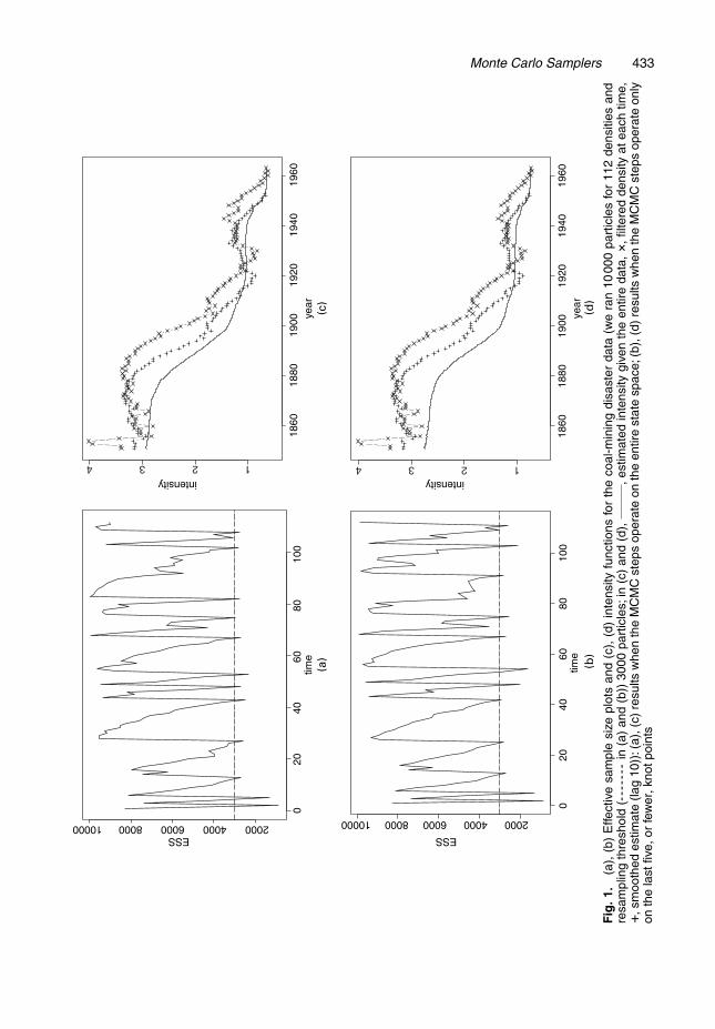
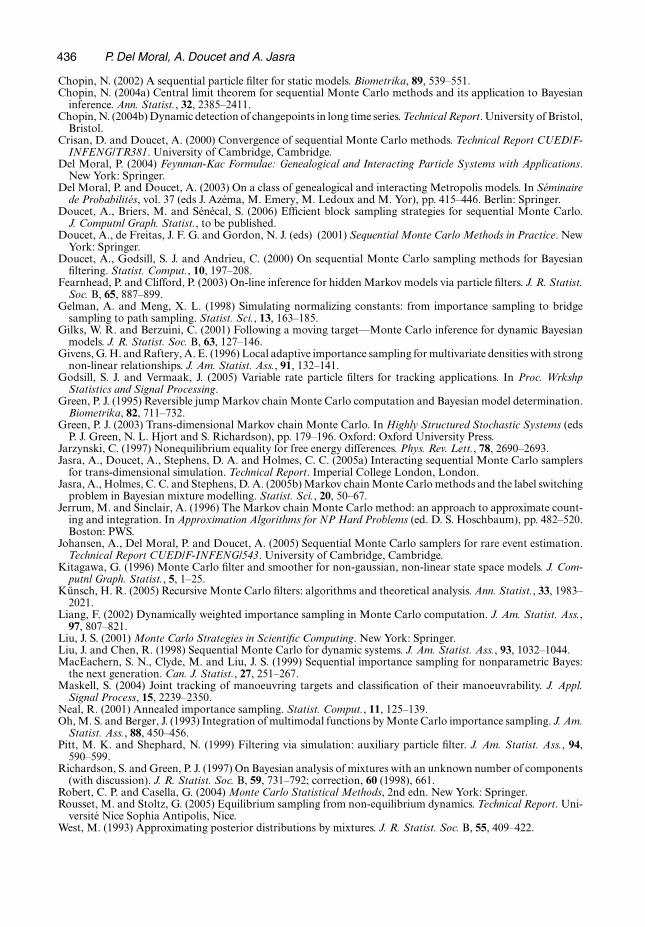
Fig. 1(a) demonstrates the performance of our algorithm with respect to weight degener-acy. Here we see that, after the initial difficulty of the sampler (due to the initialization fromthe prior, and the targets’ dynamic nature—we found that using more MCMC sweeps did notimprove the performance) the ESS never drops below 25% of its previous value. Additionally,we resample, on average, every 8.33 time steps. These statements are not meaningless whenusing resampling. This is because we found, for less efficient forward and backward kernels,that the ESS would drop to 1 or 2 if consecutive densities had regions of high probability massin different areas of the support. Thus the plot indicates that we can indeed extend the space inan efficient manner.
Fig. 1(c) shows the intensity function for the final density (full curve) in the sequence, thefiltered density at each time point (i.e. E{λ.tn/|y1:cn}, the crosses) and the smoothed estimate,up to lag 10 (E{λ.tn/|y1:cn+10}, the pluses). We can see, as expected, that the smoothed intensityapproaches the final density, with the filtered intensity displaying more variability. We foundthat the final rate was exactly the same as Green’s (1995) transdimensional MCMC sampler forour target density.
Figs 1(b) and 1(d) illustrate the performance when we only allow the MCMC steps to operateon the last five knot points. This will reduce the amount of central processor unit time that isdevoted to sampling the particles and will allow us to consider a truly realistic on-line imple-mentation. This is of interest for large data sets. Here, we see (in Fig. 1(b)) a similar number ofresampling steps to those in Fig. 1(a). In Fig. 1(d), we observe that the estimate of the intensityfunction suffers (slightly), with a more elongated structure at later times (in comparison withFig. 1(c)), reflecting the fact that we cannot update the values of early knots in light of new data.
5.4. Summarizing remarksIn this example we have presented an application of SMC samplers to a transdimensional,sequential inference problem in Bayesian statistics. We successfully applied our methodologyto the coal-mining disaster data set.
Monte Carlo Samplers 433
year
intensity
1860
1880
1900
1920
1940
1960
(b)
(d)
(c)
(a)
ESS
200040006000800010000
year
intensity
1860
1880
1900
1920
1940
1960
time
ESS
020
4060
8010
0
time
020
4060
8010
0
200040006000800010000
Fig
.1.
(a),
(b)
Effe
ctiv
esa
mpl
esi
zepl
ots
and
(c),
(d)
inte
nsity
func
tions
for
the
coal
-min
ing
disa
ster
data
(we
ran
1000
0pa
rtic
les
for
112
dens
ities
and
resa
mpl
ing
thre
shol
d(-
----
--in
(a)
and
(b))
3000
part
icle
s;in
(c)
and
(d),
,est
imat
edin
tens
itygi
ven
the
entir
eda
ta,�
,filte
red
dens
ityat
each
time,
C,sm
ooth
edes
timat
e(la
g10
)):(
a),(
c)re
sults
whe
nth
eM
CM
Cst
eps
oper
ate
onth
een
tire
stat
esp
ace;
(b),
(d)
resu
ltsw
hen
the
MC
MC
step
sop
erat
eon
lyon
the
last
five,
orfe
wer
,kno
tpoi
nts
434 P. Del Moral, A. Doucet and A. Jasra
One point of interest is the performance of the algorithm if we cannot use the backwardkernel (25) in the extend step for alternative likelihood functions. We found that not performingthe integration and using the approximation idea in equations (28) and (29) could still lead togood performance; this idea is also useful for alternative problems such as optimal filtering fornon-linear, non-Gaussian state space models (Doucet et al., 2006).
6. Conclusion
SMC algorithms are a class of flexible and general methods to sample from distributions andto estimate their normalizing constants. Simulations demonstrate that this set of methods ispotentially powerful. However, the performances of these methods are highly dependent on thesequence of targets {πn}, forward kernels {Kn} and backward kernels {Ln}.
In cases where we want to use SMC methods to sample from a fixed target π, it would beinteresting—in the spirit of path sampling (Gelman and Meng, 1998)—to obtain the optimalpath (in the sense of minimizing the variance of the estimate of the ratio of normalizing constants)for moving from an easy-to-sample distribution π1 to πp =π. This is a very difficult problem.Given a parameterized family {πθ.t/}t∈.0,1/ such that πθ.0/ is easy to sample and πθ.1/ = π, amore practical approach consists of monitoring the ESS to move adaptively on the path θ.t/;see Johansen et al. (2005) for details.
Finally, we have restricted ourselves here to Markov kernels {Kn} to sample the particles.However, it is possible to design kernels whose parameters are a function of the whole set ofcurrent particles as suggested in Crisan and Doucet (2000), Cappe et al. (2004), Chopin (2002)or West (1993). This allows the algorithm to scale a proposal distribution automatically. Thisidea is developed in Jasra et al. (2005a).
Acknowledgements
The authors are grateful to their colleagues and the reviewers for their comments which allowedus to improve this paper significantly. The second author is grateful to the Engineering andPhysical Sciences Research Council and the Institute of Statistical Mathematics, Tokyo, Japan,for their support. The third author thanks Dave Stephens and Chris Holmes for funding andadvice related to this paper.
Appendix A
A.1. Proof of proposition 1The result follows easily from the variance decomposition formula
var{wn.X1:n/}=E[var{wn.X1:n/|Xn}]+var[E{wn.X1:n/|Xn}]: .42/
The second term on the right-hand side of equation (42) is independent of the backward Markov kernels{Lk} as
E{wn.X1:n/|Xn}=γn.Xn/=ηn.Xn/
whereas var{w.X1:n/|Xn} is equal to 0 if we use equation (21).
A.2. Proof of proposition 2Expression (35) follows from the delta method. Expression (37) follows from a convenient rewriting of thevariance expression that was established in Del Moral (2004), proposition 9.4.2, page 302; see also Chopin(2004a), theorem 1, for an alternative derivation. The variance is given by
Monte Carlo Samplers 435
σ2SMC,n.ϕ/=Eη1 [w2
1 Q2:n{ϕ−Eπn .ϕ/}2]+n∑
k=2Eπk−1Kk
[w2k Qk+1:n{ϕ−Eπn .ϕ/}2] .43/
where the semigroup Q is defined as Qn+1:n.ϕ/=ϕ,
Qk+1:n.ϕ/=Qk+1 ◦ . . .◦Qn.ϕ/
and
Qn.ϕ/.xn−1/=EKn.xn−1, ·/{wn.xn−1, Xn/ϕ.Xn/}where
wn.xn−1, xn/= πn.xn/Ln−1.xn, xn−1/
πn−1.xn−1/Kn.xn−1, xn/
= Zn−1
Zn
wn.xn−1, xn/:
Expression (43) is difficult to interpret. It is conveniently rearranged here. The key is to note that
Qn.ϕ/.xn−1/=EKn.xn−1,·/{wn.xn−1, Xn/ϕ.Xn/}
=∫
Kn.xn−1, xn/πn.xn/Ln−1.xn, xn−1/
πn−1.xn−1/Kn.xn−1, xn/ϕ.xn/ dxn
= 1πn−1.xn−1/
∫ϕ.xn/πn.xn/Ln−1.xn, xn−1/ dxn
= πn.xn−1/
πn−1.xn−1/
∫ϕ.xn/ πn.xn|xn−1/ dxn:
Similarly, we obtain
Qn−1:n.ϕ/=Qn−1{Qn.ϕ/}.xn−1/
=EKn−1.xn−2,·/{wn−1.xn−2:n−1/Qn.ϕ/.xn−1/}
= 1πn−2.xn−2/
∫ {1
πn−1.xn−1/
∫ϕ.xn/πn.xn/Ln−1.xn, xn−1/ dxn
}πn−1.xn−1/Ln−2.xn−1, xn−2/ dxn−1
= 1πn−2.xn−2/
∫ {∫ϕ.xn/ πn.xn−1:n|xn−2/ dxn−1:n
}πn−2.xn−2/ dxn−1
= πn−1.xn−2/
πn−2.xn−2/
∫ϕ.xn/ πn.xn|xn−2/ dxn
and, by induction, we obtain
Qk+1:n.ϕ/= 1πk.xk/
∫· · ·
∫ϕ.xn/πn.xn/
n−1∏i=k
Li.xi, xi−1/ dxk+1:n .44/
= πn.xk/
πk.xk/
∫ϕ.xn/ πn.xn|xk/ dxn:
The expression of σ2SMC,n.ϕ/ that is given in equation (37) follows now directly from equations (44) and
(43). Similarly we can rewrite the variance expression that was established in Del Moral (2004), proposition9.4.1, page 301, and use the delta method to establish equation (38).
References
Cappe, O., Guillin, A., Marin, J. M. and Robert, C. P. (2004) Population Monte Carlo. J. Computnl Graph. Statist.,13, 907–930.
Carpenter, J., Clifford, P. and Fearnhead, P. (1999) An improved particle filter for non-linear problems. IEE Proc.Radar Sonar Navign, 146, 2–7.
Celeux, G., Marin, J. M. and Robert, C. P. (2006) Iterated importance sampling in missing data problems. To bepublished.
436 P. Del Moral, A. Doucet and A. Jasra
Chopin, N. (2002) A sequential particle filter for static models. Biometrika, 89, 539–551.Chopin, N. (2004a) Central limit theorem for sequential Monte Carlo methods and its application to Bayesian
inference. Ann. Statist., 32, 2385–2411.Chopin, N. (2004b) Dynamic detection of changepoints in long time series. Technical Report. University of Bristol,
Bristol.Crisan, D. and Doucet, A. (2000) Convergence of sequential Monte Carlo methods. Technical Report CUED/F-
INFENG/TR381. University of Cambridge, Cambridge.Del Moral, P. (2004) Feynman-Kac Formulae: Genealogical and Interacting Particle Systems with Applications.
New York: Springer.Del Moral, P. and Doucet, A. (2003) On a class of genealogical and interacting Metropolis models. In Seminaire
de Probabilites, vol. 37 (eds J. Azema, M. Emery, M. Ledoux and M. Yor), pp. 415–446. Berlin: Springer.Doucet, A., Briers, M. and Senecal, S. (2006) Efficient block sampling strategies for sequential Monte Carlo.
J. Computnl Graph. Statist., to be published.Doucet, A., de Freitas, J. F. G. and Gordon, N. J. (eds) (2001) Sequential Monte Carlo Methods in Practice. New
York: Springer.Doucet, A., Godsill, S. J. and Andrieu, C. (2000) On sequential Monte Carlo sampling methods for Bayesian
filtering. Statist. Comput., 10, 197–208.Fearnhead, P. and Clifford, P. (2003) On-line inference for hidden Markov models via particle filters. J. R. Statist.
Soc. B, 65, 887–899.Gelman, A. and Meng, X. L. (1998) Simulating normalizing constants: from importance sampling to bridge
sampling to path sampling. Statist. Sci., 13, 163–185.Gilks, W. R. and Berzuini, C. (2001) Following a moving target—Monte Carlo inference for dynamic Bayesian
models. J. R. Statist. Soc. B, 63, 127–146.Givens, G. H. and Raftery, A. E. (1996) Local adaptive importance sampling for multivariate densities with strong
non-linear relationships. J. Am. Statist. Ass., 91, 132–141.Godsill, S. J. and Vermaak, J. (2005) Variable rate particle filters for tracking applications. In Proc. Wrkshp
Statistics and Signal Processing.Green, P. J. (1995) Reversible jump Markov chain Monte Carlo computation and Bayesian model determination.
Biometrika, 82, 711–732.Green, P. J. (2003) Trans-dimensional Markov chain Monte Carlo. In Highly Structured Stochastic Systems (eds
P. J. Green, N. L. Hjort and S. Richardson), pp. 179–196. Oxford: Oxford University Press.Jarzynski, C. (1997) Nonequilibrium equality for free energy differences. Phys. Rev. Lett., 78, 2690–2693.Jasra, A., Doucet, A., Stephens, D. A. and Holmes, C. C. (2005a) Interacting sequential Monte Carlo samplers
for trans-dimensional simulation. Technical Report. Imperial College London, London.Jasra, A., Holmes, C. C. and Stephens, D. A. (2005b) Markov chain Monte Carlo methods and the label switching
problem in Bayesian mixture modelling. Statist. Sci., 20, 50–67.Jerrum, M. and Sinclair, A. (1996) The Markov chain Monte Carlo method: an approach to approximate count-
ing and integration. In Approximation Algorithms for NP Hard Problems (ed. D. S. Hoschbaum), pp. 482–520.Boston: PWS.
Johansen, A., Del Moral, P. and Doucet, A. (2005) Sequential Monte Carlo samplers for rare event estimation.Technical Report CUED/F-INFENG/543. University of Cambridge, Cambridge.
Kitagawa, G. (1996) Monte Carlo filter and smoother for non-gaussian, non-linear state space models. J. Com-putnl Graph. Statist., 5, 1–25.
Kunsch, H. R. (2005) Recursive Monte Carlo filters: algorithms and theoretical analysis. Ann. Statist., 33, 1983–2021.
Liang, F. (2002) Dynamically weighted importance sampling in Monte Carlo computation. J. Am. Statist. Ass.,97, 807–821.
Liu, J. S. (2001) Monte Carlo Strategies in Scientific Computing. New York: Springer.Liu, J. and Chen, R. (1998) Sequential Monte Carlo for dynamic systems. J. Am. Statist. Ass., 93, 1032–1044.MacEachern, S. N., Clyde, M. and Liu, J. S. (1999) Sequential importance sampling for nonparametric Bayes:
the next generation. Can. J. Statist., 27, 251–267.Maskell, S. (2004) Joint tracking of manoeuvring targets and classification of their manoeuvrability. J. Appl.
Signal Process, 15, 2239–2350.Neal, R. (2001) Annealed importance sampling. Statist. Comput., 11, 125–139.Oh, M. S. and Berger, J. (1993) Integration of multimodal functions by Monte Carlo importance sampling. J. Am.
Statist. Ass., 88, 450–456.Pitt, M. K. and Shephard, N. (1999) Filtering via simulation: auxiliary particle filter. J. Am. Statist. Ass., 94,
590–599.Richardson, S. and Green, P. J. (1997) On Bayesian analysis of mixtures with an unknown number of components
(with discussion). J. R. Statist. Soc. B, 59, 731–792; correction, 60 (1998), 661.Robert, C. P. and Casella, G. (2004) Monte Carlo Statistical Methods, 2nd edn. New York: Springer.Rousset, M. and Stoltz, G. (2005) Equilibrium sampling from non-equilibrium dynamics. Technical Report. Uni-
versite Nice Sophia Antipolis, Nice.West, M. (1993) Approximating posterior distributions by mixtures. J. R. Statist. Soc. B, 55, 409–422.