Semi-Numerical Method for Calculation of Loss in Foil ... · Semi-Numerical Method for Calculation...

IEEJ Journal of Industry ApplicationsVol.4 No.4 pp.301–309 DOI: 10.1541/ieejjia.4.301

Paper

Semi-Numerical Method for Calculation of Loss in Foil WindingsExposed to an Air-Gap Field

David Leuenberger∗a)Non-member, Jurgen Biela∗ Non-member

(Manuscript received July 28, 2014, revised Dec. 22, 2014)

The calculation of eddy current losses in foil windings exposed to a 2-D fringing field is a complex task becauseof the current displacement along the height of the foil. For model-based optimization of magnetic components, losscalculation with 2-D finite element method simulation is not an option because of the high computational effort. Theexisting alternative calculation methods with low computational effort, rely on approximations applicable only to a cer-tain geometrical arrangement of the windings and the air gap. Therefore, in this study, a new semi-numerical methodwas developed to overcome these limitations. The method is based on the mirroring method and is applicable to ar-bitrary air gaps and winding arrangements. The accuracy of the new method was verified by measurements, and thedeviation of the model results from the measured losses was found to be below 15%.

Keywords: air-gap fringing field, eddy current losses, foil winding, magnetic components

1. Introduction

Foil windings feature better thermal properties and a highercopper filling factor than Litz or round wires. On the otherhand, foil windings exposed to a 2-D magnetic fringing fieldare subject to current displacement in two directions, alongthe thickness thck as well as the width wdth of the foil, seethe example of a foil-inductor in Fig. 1(a) and (b). Calcu-lation methods neglecting the influence of this current dis-placement suffer from poor modeling accuracy (1) (2), as shownfor the foil-inductor in Fig. 1(c). To accurately predict thelosses in the foil windings, the current displacement must betaken into account, which requires a 2-D field calculation inthe winding window. A finite element simulation (FEM) isthe most commonly applied approach to perform this 2-Dfield calculation. Though FEM suffers from long calculationtimes and difficult parametrization (1). The work in (3), whichapplied a genetic algorithm to optimize a transformer withfoil windings, reported calculation times of 20 hours evenfor a simplified FEM model considering only one harmoniccomponent. However, for most applications it is inevitableto consider more than one harmonic component for accurateloss prediction. Therefore, FEM is not considered to be anideal option for automatized model-based optimization. Var-ious alternative methods are proposed in literature to considerthe effect of 2-D fringing fields. They can be categorized intotwo distinct approaches.

The first approach is to derive analytical formulas, whichtake into account the losses caused by the fringing field andallow for very high calculation speed. The derived formulas

This work has been published at the IPEC-Hiroshima ECCEAsia, May 18th–21th, 2014 under the same title.

a) Correspondence to: David Leuenberger. E-mail: [email protected]∗ Laboratory for High Power Electronic Systems (HPE)

ETH Zurich, Physikstrasse 3, CH-8092, Switzerland

Fig. 1. FEM Simulation of foil windings in a windingwindow of a gapped magnetic core (I f oil = 5 A/30 kHz):(a) Magnetic field (b) Non-homogeneous current densityalong foil 1 (see cut-line in Fig. 1(a). The homogeneouscurrent density would be 2.5e6 A/m2) (c) Losses in thefoil winding at 5 Arms sinusoidal winding current at dif-ferent frequencies in comparison to a simple 1D calcula-tion method (4) and the DC-losses

rely on an analytical solution of the Maxwell equations inthe winding-window. However, to obtain analytically solv-able differential-equations, approximations and restrictionsto simple geometries are required. The solid-conductor-method proposed in (1), (2) and the method proposed by (5),(6) are the most known methods of this kind. The solid-conductor-method approximates the layers of a foil-windingas one unified solid conductor. The model is shown to be

c© 2015 The Institute of Electrical Engineers of Japan. 301

Semi-Numerical Method for Calculation of Loss in Foil Windings Exposed to an Air-Gap Field（David Leuenberger et al.）

accurate for low frequencies, but at high frequencies the ac-curacy decreases, because the solid conductor exhibits differ-ent eddy currents, than a foil winding would actually have.The method described in (5), (6) approximates the eddy cur-rent as line-current-density located at the surface of the foilclosest to the gap. This foil is assumed to absorb the wholefringing field. The air-gap is also modelled as line-current-density (by Fourier-decomposition in space). For either ofthese two methods, the air-gaps must be located at the in-ner core-leg and the area between the air-gap and the foil-winding must be filled with air or a spacer only (no additionalround-conductor winding).The second approach is often referred to as semi-empiricalor semi-numerical. A closed-form formula for the losses isderived from a set of prior FEM simulations. This approachtries to combine the advantages of the FEM-approach - highaccuracy and no geometrical restrictions - and the advan-tages of the analytical-approach - high calculation speed. Thesquared-field-derivative method, proposed in (7) for round-wires is an example of such a method. The work in (8) derivesa modified Dowells-formula (4) for losses in the foil-windingof a high-frequency transformer. The formula contains addi-tional parameters, used to curve-fit the losses from 2-D FEMsimulations and enables fast calculation of winding losses.Though, it is restricted to a certain geometry, analyzed priorby FEM simulations.To be able to effectively perform model-based optimizationof magnetic components with foil windings, a method isneeded, which features much lower calculation times than aFEM-simulation and on the same time is not subject to re-strictions on air-gap and winding arrangement as the existinganalytical and semi-numerical approaches. To fulfil this need,in this work a novel, semi-numerical method is developed,which can be applied to arbitrary winding and air-gap geome-tries. Regarding calculation times, the new method is in be-tween the FEM- and the existing semi-empirical approaches.The developed method can be combined with the mirroringmethod and is a true 2-D field approximation for foil wind-ings. The method is described in Sect. 2 and its validation isgiven in Sect. 3.

2. Foil- to Square-Conductor Method

In the following the principle of the calculation method isexplained with the example of an inductor with foil wind-ings. Figure 1(a) shows a 2-D finite element simulation ofan inductor with a sinusoidal winding current of Iz, f oil =

5 A@30 kHz. |H| is the amplitude of the 2-D magnetic fieldintroduced by the air-gap. The x-component of the H-field,which is perpendicular to the foils, causes an eddy currentflowing in the y-z plane. The existence of the eddy currentsresults in an inhomogeneous current distribution Jz, which isshown in Fig. 1(b) for the foil closest to the air-gap. For accu-rate loss modelling, the investigated method must determinethe non-homogeneous Jz of every foil of the winding.The routine to perform this task, consists of two major parts.The first part is the calculation of the non-homogeneous cur-rent density Jz, f oil in a single foil by the following stepsshown in Fig. 2:

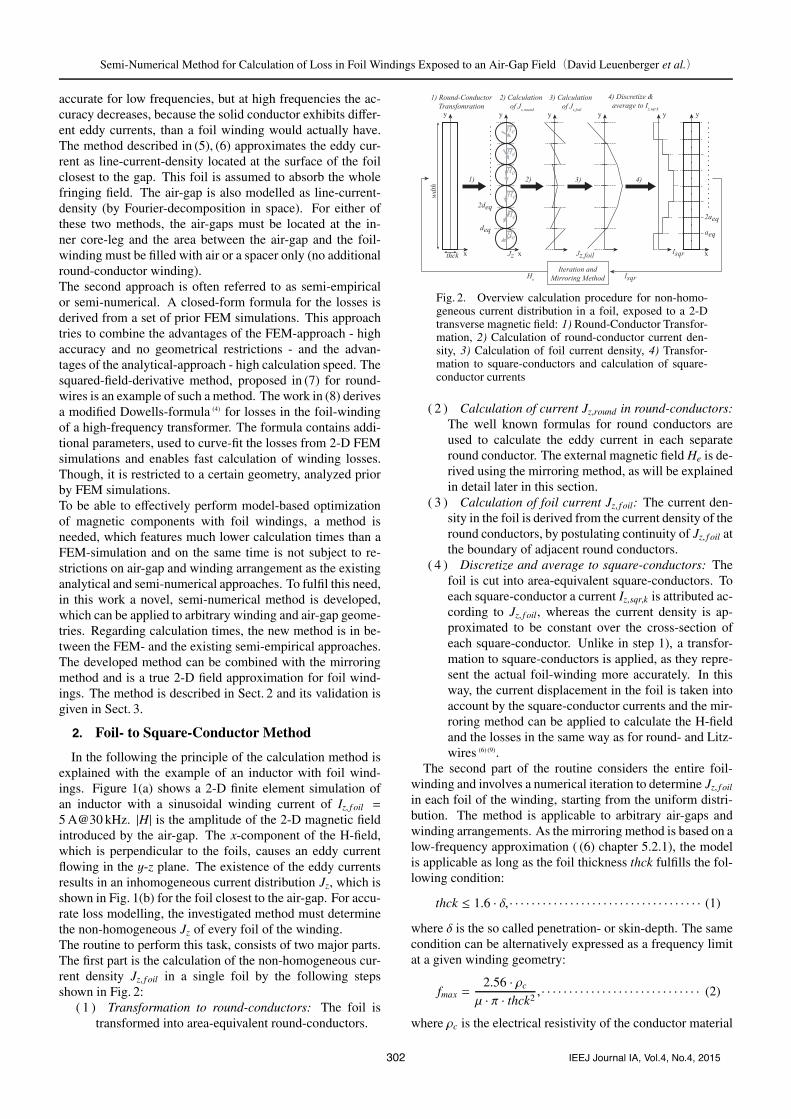
( 1 ) Transformation to round-conductors: The foil istransformed into area-equivalent round-conductors.

Fig. 2. Overview calculation procedure for non-homo-geneous current distribution in a foil, exposed to a 2-Dtransverse magnetic field: 1) Round-Conductor Transfor-mation, 2) Calculation of round-conductor current den-sity, 3) Calculation of foil current density, 4) Transfor-mation to square-conductors and calculation of square-conductor currents

( 2 ) Calculation of current Jz,round in round-conductors:The well known formulas for round conductors areused to calculate the eddy current in each separateround conductor. The external magnetic field He is de-rived using the mirroring method, as will be explainedin detail later in this section.

( 3 ) Calculation of foil current Jz, f oil: The current den-sity in the foil is derived from the current density of theround conductors, by postulating continuity of Jz, f oil atthe boundary of adjacent round conductors.

( 4 ) Discretize and average to square-conductors: Thefoil is cut into area-equivalent square-conductors. Toeach square-conductor a current Iz,sqr,k is attributed ac-cording to Jz, f oil, whereas the current density is ap-proximated to be constant over the cross-section ofeach square-conductor. Unlike in step 1), a transfor-mation to square-conductors is applied, as they repre-sent the actual foil-winding more accurately. In thisway, the current displacement in the foil is taken intoaccount by the square-conductor currents and the mir-roring method can be applied to calculate the H-fieldand the losses in the same way as for round- and Litz-wires (6) (9).

The second part of the routine considers the entire foil-winding and involves a numerical iteration to determine Jz, f oil

in each foil of the winding, starting from the uniform distri-bution. The method is applicable to arbitrary air-gaps andwinding arrangements. As the mirroring method is based on alow-frequency approximation ( (6) chapter 5.2.1), the modelis applicable as long as the foil thickness thck fulfills the fol-lowing condition:

thck ≤ 1.6 · δ, · · · · · · · · · · · · · · · · · · · · · · · · · · · · · · · · · · · (1)

where δ is the so called penetration- or skin-depth. The samecondition can be alternatively expressed as a frequency limitat a given winding geometry:

fmax =2.56 · ρc

μ · π · thck2, · · · · · · · · · · · · · · · · · · · · · · · · · · · · · (2)

where ρc is the electrical resistivity of the conductor material

302 IEEJ Journal IA, Vol.4, No.4, 2015


and μ the permeability of the material.The following two sections describe both parts of the routinein detail.2.1 Non-Homogeneous Current Density in a 2-D

Transverse Field The inhomogeneous foil current den-sity Jz, f oil caused by the 2-D transverse field He is calculatedwith the procedure shown in Fig. 2, which consists of foursteps:2.1.1 Transformation to Round-conductors The

foil-winding is transformed into a series of aligned equiv-alent round-conductors, using the equivalent DC-resistancetransformation ((6), chapter 5.4.1 and (10)) and postulatingequivalent width wdth of the transformed winding, see Fig. 2,1). The constraints on surface and width can be expressed bywdth · thck = ncond · π · (deq/2)2 and ncond · deq = wdth fromwhich follows:

deq =4 ∗ thckπ. · · · · · · · · · · · · · · · · · · · · · · · · · · · · · · · · · · (3)

2.1.2 Calculation of Current J z,round in Round-conductors With the foil decomposed into aligned roundconductors, the eddy current caused by the external magnetic

field−→He in a round conductor can be calculated using the for-

mula derived in (11) formula (7-45):

Jz(r, ϕ) = 4μ2He j32 k

J1( j32 kr)

F( j32 kreq)

sin(ϕ − ϕHe). · · · · · · · (4)

where

F( j32 kreq) = (μ1 + μ2)J0( j

32 kreq) + (μ1 − μ2)J2( j

32 kreq)

· · · · · · · · · · · · · · · · · · · · (5)

k =√

(2π f )ρ1μ1 · · · · · · · · · · · · · · · · · · · · · · · · · · · · · · · (6)

andμ1 magnetic permeability of the conductor materialρ1 conductivity of the conductor materialμ2 magnetic permeability of material around the conduc-

tor−→He sinusoidal transverse magnetic field vector with am-

plitude He and ϕHe

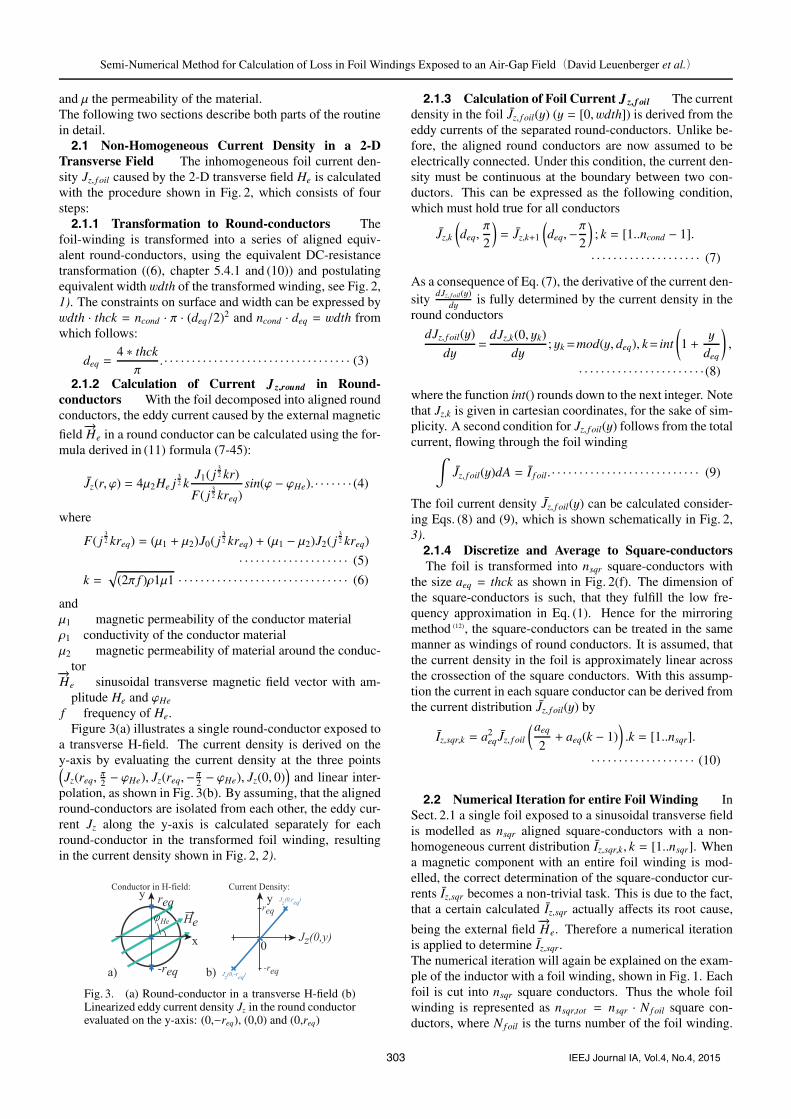
f frequency of He.Figure 3(a) illustrates a single round-conductor exposed to

a transverse H-field. The current density is derived on they-axis by evaluating the current density at the three points(Jz(req,

π2 − ϕHe), Jz(req,− π2 − ϕHe), Jz(0, 0)

)and linear inter-

polation, as shown in Fig. 3(b). By assuming, that the alignedround-conductors are isolated from each other, the eddy cur-rent Jz along the y-axis is calculated separately for eachround-conductor in the transformed foil winding, resultingin the current density shown in Fig. 2, 2).

Fig. 3. (a) Round-conductor in a transverse H-field (b)Linearized eddy current density Jz in the round conductorevaluated on the y-axis: (0,−req), (0,0) and (0,req)

2.1.3 Calculation of Foil Current J z, f oil The currentdensity in the foil Jz, f oil(y) (y = [0, wdth]) is derived from theeddy currents of the separated round-conductors. Unlike be-fore, the aligned round conductors are now assumed to beelectrically connected. Under this condition, the current den-sity must be continuous at the boundary between two con-ductors. This can be expressed as the following condition,which must hold true for all conductors

Jz,k

(deq,π

2

)= Jz,k+1

(deq,−π2

); k = [1..ncond − 1].

· · · · · · · · · · · · · · · · · · · · (7)

As a consequence of Eq. (7), the derivative of the current den-sity dJz, f oil(y)

dy is fully determined by the current density in theround conductors

dJz, f oil(y)

dy=

dJz,k(0, yk)dy

; yk=mod(y, deq), k= int

(1 +

y

deq

),

· · · · · · · · · · · · · · · · · · · · · · · (8)

where the function int() rounds down to the next integer. Notethat Jz,k is given in cartesian coordinates, for the sake of sim-plicity. A second condition for Jz, f oil(y) follows from the totalcurrent, flowing through the foil winding∫

Jz, f oil(y)dA = I f oil. · · · · · · · · · · · · · · · · · · · · · · · · · · · (9)

The foil current density Jz, f oil(y) can be calculated consider-ing Eqs. (8) and (9), which is shown schematically in Fig. 2,3).2.1.4 Discretize and Average to Square-conductorsThe foil is transformed into nsqr square-conductors with

the size aeq = thck as shown in Fig. 2(f). The dimension ofthe square-conductors is such, that they fulfill the low fre-quency approximation in Eq. (1). Hence for the mirroringmethod (12), the square-conductors can be treated in the samemanner as windings of round conductors. It is assumed, thatthe current density in the foil is approximately linear acrossthe crossection of the square conductors. With this assump-tion the current in each square conductor can be derived fromthe current distribution Jz, f oil(y) by

Iz,sqr,k = a2eq Jz, f oil

(aeq

2+ aeq(k − 1)

).k = [1..nsqr].

· · · · · · · · · · · · · · · · · · · (10)

2.2 Numerical Iteration for entire Foil Winding InSect. 2.1 a single foil exposed to a sinusoidal transverse fieldis modelled as nsqr aligned square-conductors with a non-homogeneous current distribution Iz,sqr,k, k = [1..nsqr]. Whena magnetic component with an entire foil winding is mod-elled, the correct determination of the square-conductor cur-rents Iz,sqr becomes a non-trivial task. This is due to the fact,that a certain calculated Iz,sqr actually affects its root cause,

being the external field−→He. Therefore a numerical iteration

is applied to determine Iz,sqr.The numerical iteration will again be explained on the exam-ple of the inductor with a foil winding, shown in Fig. 1. Eachfoil is cut into nsqr square conductors. Thus the whole foilwinding is represented as nsqr,tot = nsqr · Nf oil square con-ductors, where Nf oil is the turns number of the foil winding.



Fig. 4. Overview numerical iteration for calculation of the non-homogeneous current distribution in foilwindings

Fig. 5. Numeric iteration for the current in foil 1 of the inductor with foil-winding (shown in Fig. 1): Isqr,k andIsqr,calc at different iteration-steps in comparison to the current distribution Isqr,FEM derived from the 2-D FEMsimulation of the inductor

For the winding loss calculation, an arbitrary winding currentwaveform i f oil(t) is decomposed into its complex spectrumby means of the Fourier transform. For each harmonic I f oil

at frequency fh, the iteration must be performed separately.The complex array Isqr of size (1 x nsqr,tot) contains the cur-rent amplitudes of all square conductors. The starting pointof the iteration is the uniform current-distribution:

Isqr,0 =

[I f oil

nsqr. . .

I f oil

nsqr

]. · · · · · · · · · · · · · · · · · · · · · · · · · (11)

Figure 4 shows the overview of the numeric iteration. At thekth iteration, the latest current-distribution Isqr,k is used as in-put to the mirroring method, to calculate the external H-fieldat the position of each square conductor He,x and He,y. Withthe foil-to-square-conductor method described in Sect. 2.1,the current distribution Isqr,calc, that is caused by this exter-nal field, is calculated. The expression

Isqr,k = Isqr,calc. · · · · · · · · · · · · · · · · · · · · · · · · · · · · · · · · · (12)

is a sufficient condition for the correct current distribution.It describes the situation, where the physical root cause andits effect are in balance. Due to the miscellaneous approxi-mations involved in this method, condition Eq. (12) can notbe exactly fulfilled. The goal of the iteration is therefore tominimize the error

esqr =| Isqr,calc − Isqr,k | . · · · · · · · · · · · · · · · · · · · · · · · · · (13)

This minimization could as well be treated as a purelymathematical problem and state of the art algorithms could beused to determine Isqr. Though the investigation of such algo-rithms and the comparison of their performance to the appliediteration-method is out of scope for this work. The applied it-erative calculation method for Isqr is based on a control-loop

analogy. Further it is taken advantage of the fact, that the cal-culated current distribution Isqr,calc exhibits, apart from a pro-portional scaling factor, approximately the same waveform asthe correct current distribution Isqr,end. This makes it possibleto adjust Isqr,k by adding an increment Isqr,incr derived fromesqr at each iteration. Figure 5 illustrates this on the exampleof the inductor, shown in Fig. 1. The norm of the current dis-tributions in foil 1, |Isqr,k | and |Isqr,calc | are shown at the verybeginning of the iteration and after 5 and 10 iteration steps.The current distribution, |Isqr,FEM |, derived from a 2-D FEMsimulation, is shown as comparison. From the first iterationstep on, |Isqr,calc| and |Isqr,FEM | exhibit similar waveforms and|Isqr,k | approaches |Isqr,FEM | with advancing iteration.

The detailed function to determine Iincr from esqr is splitinto three parts, shown in Fig. 4, which are described in thefollowing:• Variable Gain Controller: To iteratively reduce the error

esqr, the current distribution is incremented byΔIsqr = pk · esqr. · · · · · · · · · · · · · · · · · · · · · · · · · · · (14)

•Gain Adjustment: The proportional gain pk is adjusted ineach iteration step, in order to limit the maximal currentincrement per iteration step to Istep,max,k, hence

pk =Istep,max,k

max(esqr). · · · · · · · · · · · · · · · · · · · · · · · · · · · (15)

The limit Istep,max,k is initialized to the uniform currentdistribution

Istep,max,0 =I f oil

nsqr. · · · · · · · · · · · · · · · · · · · · · · · · · · (16)

During iteration Istep,max,k is stepwise reduced to ensure,that esqr converges. If the averaged error over the wholewinding esqr,avg,k =

∑esqr,k/nsqr,tot did not diminish com-

pared to the error at the last iteration esqr,avg,k−1, thanIstep,max is adjusted:



(esqr,avg,k > esqr,avg,k−1)⇒Istep,max,k+1 =

Istep,max,k

2.· · · · · · · · · · · · · · · · · · (17)

• Phase Decoupling: The feedback-loop introducesa phase-shift, see equation 4 of the foil-to-square-conductor method. To ensure, that the current incre-ment ΔIsqr will actually compensate for the error esqr,the phase-shift of the current increment must be com-pensated by:

Iincr = ΔIsqr · e− jϕcalc . · · · · · · · · · · · · · · · · · · · · · · · (18)where ϕcalc is the phase-shift of the foil-to-square-conductor method given by:ϕcalc = ∠Isqr,calc − ∠Isqr,k. · · · · · · · · · · · · · · · · · · · (19)

The iteration loop is executed and the current distributionis adjusted by

Isqr,k+1 = Isqr,k + Iincr · · · · · · · · · · · · · · · · · · · · · · · · · · · (20)

until esqr converges to a negligible small value, having aninsignificant influence on the calculated winding losses. Al-ternatively the winding losses in the whole foil winding canbe directly taken as convergence criteria.

Pf oil,tot,k =

nsqr,tot∑k=1

Psqr,k, · · · · · · · · · · · · · · · · · · · · · · · · · (21)

ΔP,k = 100|Pf oil,tot,k − Pf oil,tot,k−1 |

|Pf oil,tot,k | · · · · · · · · · · · · · · · (22)

where Psqr,k are the eddy current losses in the kth square-conductor calculated as described in (6). The iteration isstopped, if ΔP,k stays below a certain threshold over 5 iter-ations:

max(ΔP,k−5, . . . ,ΔP,k) ≤ 0.1%⇒ Stop · · · · · · · · · · · (23)

3. Validation of the Proposed Method

The proposed method is validated on the example of aflyback-transformer for a PV-inverter. The whole calcula-tion routine, including the foil-to-square-conductor method,is implemented as software program. The losses in the con-ductors are calculated according to (13), for Litz-wires, and(6), for square-conductors. The air-gap fringing field is mod-elled according to (12). The Fourier decomposition of theflyback winding-currents is performed according to (10).

It is important to keep in mind, that the mirroring methodrestricts the validity of the calculated losses. For accurate cal-culation of the magnetic field in the winding window Eq. (1)must be fulfilled. This constraint results in a frequencylimit fmax, that can be calculated for the considered flyback-transformer using Eq. (2). Above this frequency limit the mir-roring method overestimates the magnetic field in the wind-ing window and hence the calculated winding losses are sub-ject to a modeling error. Note that a transformer or inductordesign, optimized for low winding losses, generally fulfillsEq. (1). Hence Eqs. (1), (2) do not restrict the applicability ofthe proposed method for a practical design.

The validation is performed twofold, first with a FEMsimulation and second with measured losses of a flyback-transformer.

Table 1. Parameters 2-D flyback transformer with foilsand Litz-wire

Core a = 15 mm, c = 7 mm, d = 11 mm

Winding Cu foil and Litz wiresN1=5, thckw1=0.2 mm, wdthw1 =10 mm

N2 = 50, ds,w2 = 0.1 mm, Ns = 7

Air-gap lairgap = 1mm

Fig. 6. 2-D Flyback transformer with foils and Litzwires: E-core with air-gap and ‘sps’ interleaved windingswith foils on the primary and Litz wire for the secondary

Fig. 7. Flyback-Transformer as specified in Table 1,with sinusoidal excitation of the foil-winding (Iw1 =5 A) and open circuit on the secondary: 2D FEM sim-ulation results compared to losses derived from thefoil-to-square-conductor method and the 1D calculationmethod (4)

3.1 Validation with FEM Simulation The model forfoil-winding losses is compared to the conduction losses de-rived from a 2-D FEM simulation. The specification of themodelled transformer is given in Table 1 and the 2-D wind-ing arrangement is illustrated in Fig. 6. The range of validityfor the low frequency approximation of the mirroring methodgiven by Eq. (2), is fmax,w1 = 270 kHz for the foil winding andfmax,w2 = 1 MHz for the Litz-wire winding.A first validation of the loss calculation is performed for thecase of a sinusoidal current of 5 A and various frequenciesfrom 10 kHz to 10 MHz flowing through the foil winding.Whereas winding two is an open circuit. The deviation ofthe new loss model to the 2D FEM simulation is shown inFig. 7 (in percentage, normed to the FEM simulation values).The losses calculated with the new loss model exhibit goodaccordance to the 2D FEM simulation. The difference is be-low 7%, as long as the low frequency approximation is valid,and up to 15% in the whole considered frequency range. Fig-ure 7 further shows the foil losses derived from the simple 1Dcalculation method (4). In the frequency range up to 400 kHz,where a typical flyback converter would operate, this methodexhibits deviations up to 40% compared to the FEM simula-tion. For the investigated transformer geometry, the influenceof the airgap becomes negligible in the MHz-range with thetwo methods predicting approximately the same losses.



Fig. 8. Loss-calculation for flyback-transformer as spec-ified in Table 1: Iteration convergence of the windinglosses in the foil winding Pf oil,totk,k (see Eq. (21)) and theerror in the current distribution esqr,avg,k (averaged over allharmonics and normed to I f oil,rms, the foil rms-current, seeEq. (13))

Table 2. Comparison foil-to-square-conductor methodto 2D FEM simulation for flyback transformer windinglosses

Calculation Method2D FEM Foil-to-Square-Cond.

Simulation Method

ComputerLaptop, Intel-Core

[email protected] GHzCalculation time 320 s 19 s 113 s

Number of Harmonics 20 20 100Number of Iterations - 43 42

Winding Losses Pw1 1.32 W 1.28 W 1.33 WWinding Losses Pw2 0.576 W 0.575 W 0.67 W

The second validation is done by considering actual wind-ing current waveforms of a DC-DC flyback converter oper-ating in boundary conduction mode (BCM) at a switchingfrequency of 100 kHz (8 A peak, 0.75 duty cycle). To limitthe FEM calculation time, only harmonics from 100 kHz to2 MHz are considered. Figure 8 shows the convergence ofthe error in the non-homogeneous current density esqr,avg,k

and the total foil winding losses Pf oil,tot,k during the itera-tion (see Sect. 2.2). The error esqr,avg,k converges step-by-stepand decreases below 3% after 40 iterations. Simultaneouslythe calculated losses converge to the final value. After 43iterations the convergence criteria for the calculated lossesEq. (23) is fulfilled. The final value is 1.28 W, which cor-responds to a difference of 3.5% compared to the 2D FEMsimulation, see Table 2. To demonstrate the increase in cal-culation time, a second calculation-run of the foil-to-square-conductor method is performed and also listed in Table 2, tak-ing into account a larger number of harmonics from 100 kHz–10 MHz. The winding losses in the foil increase marginallyby 4% due to the higher order harmonic currents.3.2 Validation with Measured Flyback TransformerThe model for foil-winding losses is verified by measure-

ments on a flyback transformer. The transformer is builtwith a gapped RM low-profile core and foil windings onthe primary and Litz wire on the secondary. First, the mea-surement setup is described in the following paragraph. Themeasurement results and the comparison are presented in3.2.2.

Fig. 9. Experimental setup for winding loss measure-ment of the flyback transformer.

Fig. 10. Overview measurement method for core- andwinding-loss measurement of a magnetic component, ac-cording to (14)

Table 3. Winding loss measurement setup: used equip-ment

Waveform Generator Agilent 33522APower Amplifier AE Techtron 7224

Oscilloscope LeCroy WaveSurfer 24MXSBVoltage Probes LeCroy PP008Current Probe LeCroy AP015

3.2.1 Winding Loss Measurement Method and SetupThe measurement-methods proposed in (14) are applied

for this verification, which allow to derive the losses in thefoil-winding at a sinusoidal winding-current. Figure 9 showsthe measurement setup consisting of the flyback transformerand a resonance capacitor. The schematic of the entire mea-surement setup is shown in Fig. 10 and the applied measure-ment equipment is listed in Table 3. The primary windingis put in series with a capacitor Cres to form a resonant cir-cuit together with the transformers magnetizing inductance.A sinusoidal voltage source, realised with a signal generatorand a power amplifier, drives the test current Itest through theprimary winding. The secondary Litz-winding is left opencircuit. The transformer has an additional sensing-winding(0.1 mm2 Cu round-wire) having the same turns-ratio as theprimary winding, which is used for voltage measurementsonly. Hence no net current is flowing through the sensing-winding. The losses in the sensing winding are negligiblysmall, due to the low turns-number and the small conductordiameter.

The schematic in Fig. 10 shows the T-equivalent circuit ofthe transformer, the parasitic cable inductance LCable and theresonance capacitor series resistance RCES R. The equivalentcomponents of the sensing winding are not relevant, becausethe winding does not carry any current. Lσ and Lmag arethe magnetizing- and stray-inductance referred to the primary



winding. The resistors RCore and Rwdg model the losses in thecore and the primary winding. The aim of the setup is to de-termine the resistive losses in Rwdg. This can be achieved bytwo distinct measurements.• The Resonant Method as proposed in (15) and described

in (14) section 1.2.4, allows to determine the total re-sistive losses of the resonant-circuit by operating thevoltage-source at

fr =1

2π√

(Lmag + Lσ)Cr

. · · · · · · · · · · · · · · · · · · ·(24)

At this operating point the voltage over Lσ, Lmag and Cr

cancel out and the voltage measured at the input of theresonant circuit VLC only contains the resistive parts

VLC = VR,wdg + VR,core + VR,C,ES R. · · · · · · · · · · · (25)Consequently, the losses in the resonance circuit can besplit into three parts

PLC = PR,wdg + PR,core + PR,C,ES R. · · · · · · · · · · (26)The losses caused by the resonance current PLC, f r can becalculated from the measured voltage VLC and current IT

by

PLC, f r =12

IT, f rVLC, f r cos(ϕI,T, f r − ϕV,LC, f r),

· · · · · · · · · · · · · · · · · (27)where IT, f r, ϕI,T, f r and VLC, f r, ϕV,LC, f r are the amplitudeand phase at the resonance frequency derived from thefourier transform.• The Capacitive Cancellation Core Loss Method pro-

posed in (14) Sect. 2.1.2, can be applied to measure thecore losses separately. Unlike the resonant method,where the winding losses are included in the measuredlosses. The voltage Vcore is measured between the up-per port of the sensing winding to ground, as shown inFig. 10. Note that the lower port of the sensing windingis connected to the resonance capacitor and hence Vcore

can be expressed asVcore = VR,core + VL,mag + VR,C,ES R + VC,r.

· · · · · · · · · · · · · · · · · (28)The frequency of the voltage-source is chosen, such thatVL,mag = −VC,r, which is the case at

fr =1

2π√

LmagCr

. · · · · · · · · · · · · · · · · · · · · · · · · · (29)

The measured voltage only contains the resistive partsVcore = VR,core + VR,C,ES R and the resistive losses causedby the resonance current can be calculated by:

Pcore, f r =12

IT, f rVcore, f r cos(Δϕ f r), · · · · · · · · · · (30)

withΔϕ f r = ϕI,T, f r − ϕV,core, f r. · · · · · · · · · · · · · · · · · · (31)

The losses consists of the following two partsPcore, f r = PR,core, f r + PR,C,ES R, f r. · · · · · · · · · · · · (32)

To obtain the magnetic losses PR,wdg, f m at a certain fre-quency fm the losses PLC, f m and Pcore, f m are measured as ex-plained above. For the measured transformer the stray in-ductance Lσ is much smaller than Lmag and hence the sameresonant capacitance Cr can be used for both measurements.The magnetic losses can be obtained from the measurementswith Eqs. (27) and (32) by:

PR,wdg, f m � PLC, f m − Pcore, f m. · · · · · · · · · · · · · · · · · · · (33)

The losses in RC,ES R cancel out, though RC,ES R should not

be much higher than Rwdg to obtain a good resolution of themeasurement.

The accuracy of the performed loss measurements causedby the deviations in the current Δi, voltage- Δu and phase-angle measurements Δϕ can be deducted from Eqs. (27),(30) using the second-order Taylor-series of the cosine(cos(x) = 1 − x2

2

)and neglecting deviation-coefficients of

third order:

Δpmeas = ΔvI + VΔi + ΔvΔi − P2Δϕ2. · · · · · · · · · · · (34)

The phase-deviation follows from the time-delay between thevoltage- and current-probe by

Δϕ = 2π · 16ns · fmeas, · · · · · · · · · · · · · · · · · · · · · · · · · · (35)

whereas the time-delay is derived from a reference-measurement using a shunt-resistor. Voltage and current de-viation are found to be

Δv � 80μV,Δi � 1 mA. · · · · · · · · · · · · · · · · · · · · · · · · · (36)

This is above their theoretical resolution-limit of 63 μV and313 μA, due to the low signal-to-noise ratio at high scale-factors of the oscilloscope. An additional measurement er-ror introduced by the parasitic inter-winding capacitance, de-scribed in (14) (2.11), is found to be negligible small, due tothe relatively low measuring frequencies. The deviation inthe measured winding losses follows from Eq. (33)

Δpwdg � ΔpLC + Δpcore, · · · · · · · · · · · · · · · · · · · · · · · · (37)

where Δpcore and ΔpLC are calculated with Eq. (34).3.2.2 Loss Measurements and Comparison The

flyback transformer loss model is parameterized to modelthe measured flyback transformer. The frequency limit, upto which the low-frequency 2-D field approximation used forwinding loss calculation applies, is determined by Eq. (2) andequals

fmax,low, f req = 172 kHz · · · · · · · · · · · · · · · · · · · · · · · · · · (38)

for the investigated flyback transformer geometry. Above thisfrequency the modelled winding losses are subject to an in-creasing modelling error. In Table 4 the measured windinglosses are compared to the losses calculated with the modelat three different measuring points: 50 kHz, 100 kHz and200 kHz. Further the accuracy of the measured losses is de-termined with Eq. (37). The model exhibits a good accor-dance to the measured losses. The winding losses predictedby the model show a deviation below 15% for the measuringpoints at 50 kHz and 100 kHz. The measuring frequency of200 kHz is above fmax,low, f req and accordingly the deviationincreases to a value of 21%.

Table 4. Flyback transformer winding loss model vali-dation by comparison to measured losses

Frequency: Loss Measurements: Loss Model: Deviation:fmeas Pwdg Δpwdg Pwdg Δmodel

50 kHz 0.0136 W < ±3.9% 0.0132 W −2.6%100 kHz 0.0046 W < ±6.2% 0.0052 W 14.9%200 kHz 0.0022 W < ±7.5% 0.0026 W 21.3%



Fig. 11. Flyback transformer model (specification as inTable 1 at DC-DC BCM operation with harmonics from100 kHz to 2 MHz): calculation complexity analysis

3.3 Calculation Time and Complexity Reducingthe calculation speed was a major motivation to develop thefoil-to-square-conductor method. The achieved evaluationtime for the whole loss-model of a flyback-transformer inDC-DC BCM operation (see 3.1 and Table 1 for specifica-tions), is 19 s and 113 s for a considered number of higher or-der harmonics of nh = 20 and nh = 100 on a laptop computerequipped with an [email protected] GHz. In com-parison, the speed optimized FEM model, using the softwareFEMM 4.2, exhibits a calculation time of 320s for nh = 20,see Table 2 for details. Figure 11 shows the relative calcu-lation time of the most dominant tasks of the loss-model.The calculation complexity of the foil-to-square-conductormethod and the mirroring method scales linearly with nh andthe number of conductors, being nsqr,tot for the foil-to-squareand nsqr,tot +nwdg,2 for the mirroring method (nwdg,2 is the sec-ondary turns number). Note, that all dominant tasks are inthe iteration loop (see Fig. 4). Thus the iteration itself is themost time-consuming part of the loss-model, whose calcula-tion time depends linearly on the number of iterations nnum,it.Evaluations with different parameters showed, that the devel-oped numerical iteration needs an average of nnum,it � 45 toconverge. To further reduce calculation time, an improvediteration-method would be most effective. While nsqr,tot andnwdg,2 follow from the specifications, the number of harmon-ics nh can be chosen as low as possible, depending on the con-sidered current waveform. A further speed improvement canbe achieved in the mirroring method by reducing the num-ber of mirroring below the currently implemented 11x11 mir-rored basic winding windows.

4. Conclusion

A new semi-numerical method is developed for loss cal-culation in foil windings exposed to a 2-D fringing field.Compared to existing calculation methods it features the ad-vantage of much faster calculation speed compared to FEMsimulations. For the considered example the calculation timeis reduced by a factor of 16. At the same time the new methodis not restricted to certain geometric arrangements as the ex-isting analytical and semi-empirical methods. The analysis ofthe calculation complexity discloses the potential of furtherspeed improvement. The accuracy of the method is validatedon the example of a flyback transformer by both FEM simula-tions and measurements on a test-setup. The method exhibitsdeviations below 15% in comparison to the measured losses.

References

( 1 ) P. Wallmeier: “Improved analytical modeling of conductive losses ingapped high-frequency inductors”, IEEE Trans. on Ind. Appli., Vol.37, No.4,pp.1045–1054 (2001)

( 2 ) ——: “Automatisierte Optimierung von induktiven Bauelementen fur Strom-richteranlagen”, Ph.D. dissertation, Universitat Paderborn (2001), Shaker-Verlag, ISBN 3-8265-8777-4.

( 3 ) J. Zwysen, R. Gelagaev, J. Driesen, S. Gooossens, W. Vanvlasselaer,K. Symens, and B. Schuyten: “Multi-objective design of a close-coupled in-ductor for a three-phase interleaved 140kw dc-dc converter”, in 39th IECON,Vienna (2013)

( 4 ) P. Dowell: “Effects of eddy currents in transformer windings”, Proc. of theInstitution of Electrical Engineers, Vol.113, No.8, pp.1387–1394 (1966)

( 5 ) A. Van den Bossche and V. Valchev: “Eddy current losses and inductanceof gapped foil inductors”, in IEEE, 28th IECON An. Conference, Vol.2,pp.1190–1195 (2002)

( 6 ) ——, Inductors and Transformers for Power Electronics, CRC Press, Taylorand Francis Group (2005)

( 7 ) C. Sullivan: “Computationally efficient winding loss calculation withmultiple windings, arbitrary waveforms, and two-dimensional or three-dimensional field geometry”, IEEE Trans. on Power Electronics, Vol.16,No.1, pp.142–150 (2001)

( 8 ) F. Robert, P. Mathys, and J.-P. Schauwers: “A closed-form formula for 2Dohmic losses calculation in SMPS transformer foils”, in IEEE 14th APEC,Vol.1, pp.199–205 (1999)

( 9 ) J. Muehlethaler, J.W. Kolar, and A. Ecklebe: “Loss modeling of inductivecomponents employed in power electronic systems”, in Proc. IEEE 8th IPEC(ECCE Asia), pp.945–952 (2011)

(10) J. Zhang, W. Yuan, H. Zeng, and Z. Qian: “Simplified 2-d analytical modelfor winding loss analysis of flyback transformers”, Journal of Power Elec-tronics, Vol.12, No.6, pp.960–973 (2012)

(11) J. Lammeraner and M. Stafl: Eddy Currents, I. B. LTD, Ed. SNTL Publisherof Technical Literature (1966)

(12) J. Muehlethaler, M. Schweizer, B. Robert, J. Kolar, and A. Ecklebe: “Op-timal design of LCL harmonic filters for three-phase PFC rectifiers”, IEEETrans. on Power Electronics, Vol.28, No.7, pp.3114–3125 (2013)

(13) F. Tourkhani and P. Viarouge: “Accurate analytical model of winding lossesin round litz wire windings”, IEEE Trans. on Magnetics, Vol.37, pp.538–543(2001)

(14) M. Mingkai: “High frequency magnetic core loss study”, Ph.D. dissertation,Virginia Polytechnic Institute and State University (2013)

(15) F. Dong Tan, J. Vollin, and S. Cuk: “A practical approach for magnetic core-loss characterization”, IEEE Trans. on Power Electronics, Vol.10, pp.124–130 (1995)



David Leuenberger (Non-member) studied electrical engineering atthe Swiss Federal Institute of Technology (ETH)Zurich focusing on Power Electronics and ElectricalDrives. After receiving his MSc degree in 2008 heworked as engineer in the area of propulsion controlfor railway application. Since May 2011 he is pursu-ing his Ph.D. at the Laboratory for High Power Elec-tronic Systems, focusing on inverters for grid connec-tion of PV systems.

Jurgen Biela (Non-member) received the Diploma (with honors)from Friedrich-Alexander Universitaet Erlangen-Nuernberg, Germany, in 1999 and the Ph.D. degreefrom ETH Zurich, Switzerland, in 2006. Duringhis studies, he dealt in particular with resonant dc-link inverters at the University of Strathclyde, Glas-gow, U.K., and the active control of series-connectedIGCTs at the Technical University of Munich, Ger-many. In 2000, he joined the Research Department,Siemens A&D, Erlangen, where he worked on invert-

ers with very high switching frequencies, SiC components, and EMC. InJuly 2002, he joined the Power Electronic Systems Laboratory (PES), ETHZurich, for working toward his Ph.D. degree, focusing on optimized elec-tromagnetically integrated resonant converters. From 2006 to 2007, he wasa Postdoctoral Fellow with PES and a Guest Researcher with the Tokyo In-stitute of Technology, Japan. From 2007 to 2010, he was a Senior ResearchAssociate with PES. Since 2010, he has been an Associate Professor in high-power electronic systems with ETH Zurich. His current research is focusedon the design, modeling, and optimization of PFC, dc-dc and multilevel con-verters with emphasis on passive components, the design of pulsed-powersystems, and power electronic systems for future energy distribution.


Semi-Numerical Method for Calculation of Loss in Foil ... · Semi-Numerical Method for Calculation...

Documents

Transcript of Semi-Numerical Method for Calculation of Loss in Foil ... · Semi-Numerical Method for Calculation...