Semester Thesis:

Semantic Understanding of Location and Movement Informationcollected by a Mobile Application

Author: Manuel Baumannmanubaum@ee.ethz.ch

Advisor: Michael KuhnFabio Magagna

Tutor: Prof. Dr. Roger Wattenhofer

Date: January 14, 2009

Abstract

The past few years mobile devices emerged to a very important and ubiquitous communi-cation medium. They are able to handle email, multimedia contents, websites, etc. Thesame time the idea of the Web 2.0 came up. The spirit behind the Web 2.0 is thateverybody is invited to share his/her knowledge1 with the rest of the world. One logicalconsequence is the melt down of these two technologies. Social platforms on mobile de-vices will be the killer application of mobile devices. We aim to build a framework forthe location and movement awareness of these devices. This adds further value to ourmobile devices, because we could gain lots of information about a user’s situation. Thisthesis focuses on processing real-time logged data consisting of WLAN occurrences, GSMcells and GPS data for finding out how a user moves and where he/she is located. Allthe computations are done on a server. We compute five characteristical metrics whichthen are used for movement estimation by three different approaches. We try to classifythe data in 4 different kinds of movement: standing, walking, moving by car and movingby train. To evaluate the performance of the algorithms, their classifications are testedagainst a hand kept journal. The best performing movement estimation algorithm showsa classification accuracy of 85 % and locations are recognized 87% of the time.

1In form of videos or media in general, social networking, wikis and so on.

CONTENTS I

Contents

1 Introduction 1

2 Related Work 3

3 Project Setup 4

3.1 Mobile Application . . . . . . . . . . . . . . . . . . . . . . . . . . . . . . . 4

3.2 Application Overview . . . . . . . . . . . . . . . . . . . . . . . . . . . . . . 4

3.3 Log Format . . . . . . . . . . . . . . . . . . . . . . . . . . . . . . . . . . . 5

4 Data Sources 7

4.1 Wireless Local Area Network . . . . . . . . . . . . . . . . . . . . . . . . . 7

4.1.1 Identification . . . . . . . . . . . . . . . . . . . . . . . . . . . . . . 7

4.1.2 Notation . . . . . . . . . . . . . . . . . . . . . . . . . . . . . . . . . 7

4.1.3 Availability . . . . . . . . . . . . . . . . . . . . . . . . . . . . . . . 8

4.1.4 Precision . . . . . . . . . . . . . . . . . . . . . . . . . . . . . . . . . 8

4.1.5 Remarks . . . . . . . . . . . . . . . . . . . . . . . . . . . . . . . . . 8

4.2 GSM . . . . . . . . . . . . . . . . . . . . . . . . . . . . . . . . . . . . . . . 8

4.2.1 Identification . . . . . . . . . . . . . . . . . . . . . . . . . . . . . . 8

4.2.2 Notation . . . . . . . . . . . . . . . . . . . . . . . . . . . . . . . . . 9

4.2.3 Availability . . . . . . . . . . . . . . . . . . . . . . . . . . . . . . . 9

4.2.4 Precision . . . . . . . . . . . . . . . . . . . . . . . . . . . . . . . . . 9

4.2.5 Remarks . . . . . . . . . . . . . . . . . . . . . . . . . . . . . . . . . 9

4.3 GPS . . . . . . . . . . . . . . . . . . . . . . . . . . . . . . . . . . . . . . . 10

4.3.1 Identification . . . . . . . . . . . . . . . . . . . . . . . . . . . . . . 10

4.3.2 Availability . . . . . . . . . . . . . . . . . . . . . . . . . . . . . . . 11

4.3.3 Precision . . . . . . . . . . . . . . . . . . . . . . . . . . . . . . . . . 11

4.3.4 Remarks . . . . . . . . . . . . . . . . . . . . . . . . . . . . . . . . . 11

4.4 Notation . . . . . . . . . . . . . . . . . . . . . . . . . . . . . . . . . . . . . 11

4.4.1 Definition of the Measuring Point . . . . . . . . . . . . . . . . . . . 11

4.4.2 Definition of Estimation . . . . . . . . . . . . . . . . . . . . . . . . 11

5 Data Visualization 12

5.1 Web Frontend . . . . . . . . . . . . . . . . . . . . . . . . . . . . . . . . . . 12

5.2 Manual Data Collection . . . . . . . . . . . . . . . . . . . . . . . . . . . . 13

II CONTENTS

6 Data Gathering 14

6.1 GSM,WLAN Positions . . . . . . . . . . . . . . . . . . . . . . . . . . . . . 14

6.2 WLAN Connectivity Graph . . . . . . . . . . . . . . . . . . . . . . . . . . 14

6.3 WLAN Position Approximation . . . . . . . . . . . . . . . . . . . . . . . . 14

7 Location Estimation 16

7.1 Definition of Location . . . . . . . . . . . . . . . . . . . . . . . . . . . . . 16

7.2 Location Acquisition . . . . . . . . . . . . . . . . . . . . . . . . . . . . . . 17

7.3 Implementation . . . . . . . . . . . . . . . . . . . . . . . . . . . . . . . . . 17

8 Movement Estimation 18

8.1 Movement Measurements by GPS . . . . . . . . . . . . . . . . . . . . . . . 18

8.1.1 Map Data Format . . . . . . . . . . . . . . . . . . . . . . . . . . . . 18

8.1.2 Distance to Railroads and Streets . . . . . . . . . . . . . . . . . . . 18

8.1.3 Speed Estimation . . . . . . . . . . . . . . . . . . . . . . . . . . . . 20

8.2 Movement Metrics by WLAN . . . . . . . . . . . . . . . . . . . . . . . . . 20

8.2.1 Problem Description . . . . . . . . . . . . . . . . . . . . . . . . . . 20

8.2.2 Approximation . . . . . . . . . . . . . . . . . . . . . . . . . . . . . 21

8.2.3 Practical Implementation . . . . . . . . . . . . . . . . . . . . . . . . 22

8.2.4 Summary . . . . . . . . . . . . . . . . . . . . . . . . . . . . . . . . 22

8.2.5 Remarks . . . . . . . . . . . . . . . . . . . . . . . . . . . . . . . . . 23

8.3 Movement Metrics by GSM . . . . . . . . . . . . . . . . . . . . . . . . . . 23

8.4 Movement Suggestion . . . . . . . . . . . . . . . . . . . . . . . . . . . . . . 23

8.4.1 Greedy Algorithm . . . . . . . . . . . . . . . . . . . . . . . . . . . . 24

8.4.2 Support Vector Machine Approach . . . . . . . . . . . . . . . . . . 24

8.4.3 k-Nearest Neighbor Algorithm . . . . . . . . . . . . . . . . . . . . . 25

9 Performance Analysis 26

9.1 Location Estimation Analysis . . . . . . . . . . . . . . . . . . . . . . . . . 26

9.2 Movement Estimation Analysis . . . . . . . . . . . . . . . . . . . . . . . . 26

9.2.1 Notation . . . . . . . . . . . . . . . . . . . . . . . . . . . . . . . . . 26

9.2.2 Greedy Algorithm . . . . . . . . . . . . . . . . . . . . . . . . . . . . 27

9.2.3 Support Vector Machine Classification . . . . . . . . . . . . . . . . 27

9.2.4 k Nearest Neighborhood Classification . . . . . . . . . . . . . . . . 28

10 Conclusion 30

CONTENTS III

11 Future Work 31

11.1 Massive Data Gathering . . . . . . . . . . . . . . . . . . . . . . . . . . . . 31

11.2 Mobile Application . . . . . . . . . . . . . . . . . . . . . . . . . . . . . . . 31

11.3 Server Application . . . . . . . . . . . . . . . . . . . . . . . . . . . . . . . 31

11.4 Improvement of the Classification Algorithms . . . . . . . . . . . . . . . . 31

12 Acknowledgments 32

13 Appendix 34

13.1 WLAN Range Histogram . . . . . . . . . . . . . . . . . . . . . . . . . . . . 34

13.2 WLAN Connectivity Graph Example . . . . . . . . . . . . . . . . . . . . . 34

1

1 Introduction

The success of mobile devices in the past few years and the shift of the internet towardsa platform-like information medium changed our way of communication. Many peopleprovide personal information about their daily life on social plattforms. It seems to beobvious that this kind of information exchange will be done more and more using mobiledevices.

The future services and applications on the mobile phone will be on one hand similar ason the personal computer; but must be adapted to the special features of mobile phonesto minimize the limitations and maximize the advantages of mobile phones. Some of thelimitations of mobile phones are the relatively small screen and input interface; whereassome of the advantages of mobile phones are to provide the opportunity for users to be”always online” and ”traceable”. Note that the latter advantage may also create privacyconcerns. Nevertheless, all of the advantages of mobile phone open new opportunities inthe design of service applications via mobile phone. Among the many possible serviceapplications, some experts argue that the location-based services (LBS) will become the”killer application” in the near future. Indeed, the market size for LBS has been growingin an exponential rate. The market size is estimated to be 447 Mio US$ in Asia, 622 MioUS$ in Europe and 1.3 Bio US$ in USA 2010. [9]

This semester thesis aims to extend a framework for location based services. Theseservices can and will improve the way we socialize today. They add further value to ourubiquitous mobile devices, because socializing can be improved by the knowledge aboutour current location. Much of the daily social information for example where we are,where we are going and even who we are meeting can be retrieved automatically. Amultitude of possible applications could be built on top of the framework.

The basis of our work is a project called Abakabar (Indonesian for “how are you?”) andwas founded by Fabio Magagna in a former semester thesis [1]. It does not aim to providea kind of website for mobile socializing but only the core application which consists ofa mobile software and a web service which is accessed through websites by API calls.This makes this framework interesting for other developers. From the former projecteverything but the software on the mobile phone was reimplemented for the sake of theprogrammers deeper understanding of the system.

The main topic of this thesis is movement recognition. We defined four classes of move-ment we want to distinguish: standing, walking, moving by car and moving by train. Thisis done by analyzing the occurrences of WLANs, GSM cells and, if available, GPS co-ordinates. To reach this, five metrics were introduced. The first two are measures fora user’s speed gained by analyzing WLAN and GSM occurrences. These measures arejustified by a simple mathematical model. The other three measures are retrieved fromGPS coordinates. The most intuitive measure is the user’s speed. The other two variablesare the distances to railroads and streets. These five values, later called feature-vectors,are then processed by three different algorithms for movement estimation.

2 1 INTRODUCTION

The thesis is structured as follows: First we describe the former project called Abakabar.Then follows a short overview of the basics of how the mobile software works and thenwe proceed to the later used definitions. After showing how the data is visualized, thelocation estimation part is explained. The main part deals with movement estimation. Atthe end of the thesis, we evaluate and compare the performance of the three algorithms.

3

2 Related Work

There are dozens of applications for mobile phones which try to improve sozializing.They use different approaches for doing that. Some of them rely only on the WLAN orBluetooth devices they see to distinguish which user are close-by (e.g. Geode, iCloseBy,...[11]). Other act as improved interface to a social-network. They are able to capture theuser’s activity like sitting, walking, meeting friends, etc. (CenceMe [11]). One uses a builtin accelerometer to distinguish between the actions sitting, walking and running.

We do not cover the analysis of patterns in a user’s daily life. So there is no statementwhether the user is on the way to work, or visiting a friend. Nevertheless, it is a veryinteresting topic and was analyzed in another paper. [4]

A mobile phone manufacturer looks at this topic form another aspect. They look at themobile devices as the world’s most distributed and pervasive sensing instrument. Alsobecause there are more and more built-in sensors. [10]

4 3 PROJECT SETUP

3 Project Setup

3.1 Mobile Application

As this thesis is based on an other semester-thesis written by Fabio Magagna [1], thispart shows the premises of my thesis. The system consists of a mobile application whichlogs occurrences of wireless access-points, the CGIs (Cell Global Identifier) from GSMantennas and, if available, coordinates measured by GPS in 10 second intervals. Thisdata is then transferred to a server. The application has two modes of operation. Thefirst one submits the new data every 10 seconds (online modus) using UMTS while theother mode stores all data and only transmits the data if requested by the user (offlinemode). This mode is very suitable for long time logging and allows cheap uploadingthrough WLAN. The application is written in C and runs on Symbian based mobilephones.

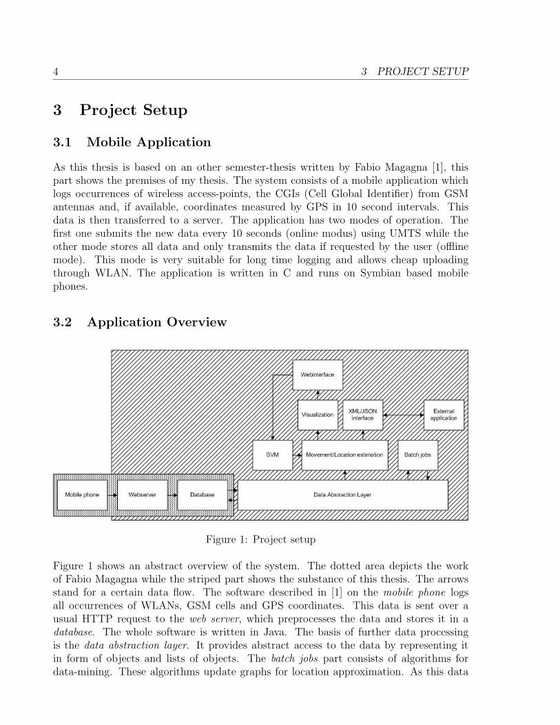
3.2 Application Overview

Figure 1: Project setup

Figure 1 shows an abstract overview of the system. The dotted area depicts the workof Fabio Magagna while the striped part shows the substance of this thesis. The arrowsstand for a certain data flow. The software described in [1] on the mobile phone logsall occurrences of WLANs, GSM cells and GPS coordinates. This data is sent over ausual HTTP request to the web server, which preprocesses the data and stores it in adatabase. The whole software is written in Java. The basis of further data processingis the data abstraction layer. It provides abstract access to the data by representing itin form of objects and lists of objects. The batch jobs part consists of algorithms fordata-mining. These algorithms update graphs for location approximation. As this data

3.3 LOG FORMAT 5

is not mandatory for the live part of the system, this data structures are only updateddaily. The Movement/Location estimation part is the core of the application. There aretwo interfaces attached to the core. The Visualization part provides visual inspection ofthe data gathered for a certain user and during a certain interval which can be displayedin any web browser. It is used to implement and verify the software. The SVM providedby libsvm [2] provides a second approach for movement estimation. The XML/JSONinterface allows access to the data in realtime for external applications.

3.3 Log Format

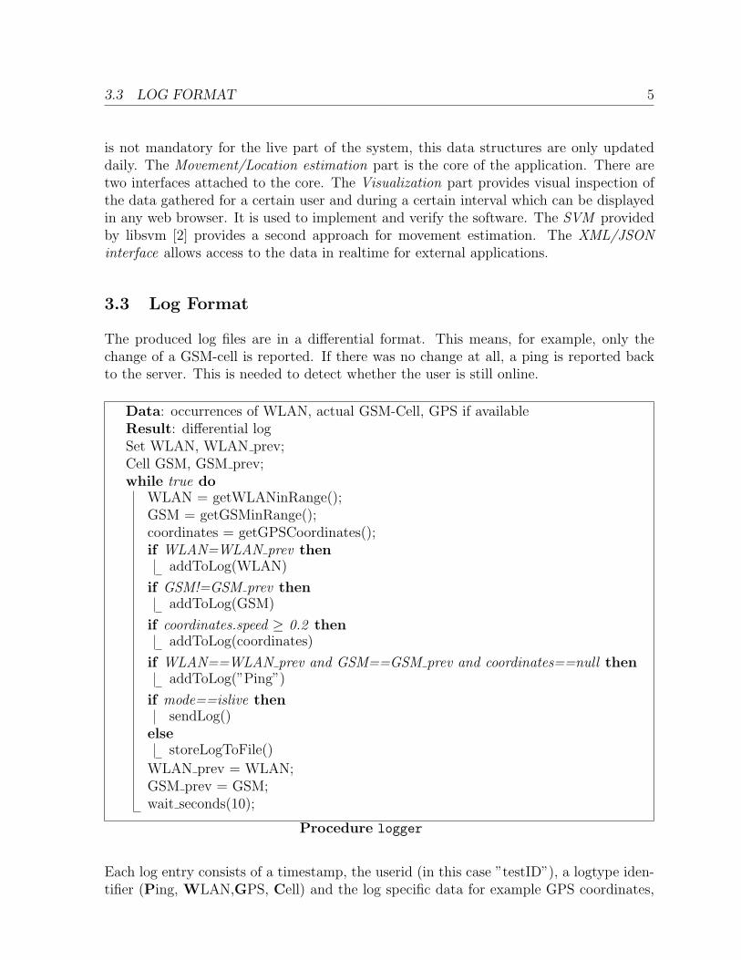
The produced log files are in a differential format. This means, for example, only thechange of a GSM-cell is reported. If there was no change at all, a ping is reported backto the server. This is needed to detect whether the user is still online.

Data: occurrences of WLAN, actual GSM-Cell, GPS if availableResult: differential logSet WLAN, WLAN prev;Cell GSM, GSM prev;while true do

WLAN = getWLANinRange();GSM = getGSMinRange();coordinates = getGPSCoordinates();if WLAN=WLAN prev then

addToLog(WLAN)

if GSM!=GSM prev thenaddToLog(GSM)

if coordinates.speed ≥ 0.2 thenaddToLog(coordinates)

if WLAN==WLAN prev and GSM==GSM prev and coordinates==null thenaddToLog(”Ping”)

if mode==islive thensendLog()

elsestoreLogToFile()

WLAN prev = WLAN;GSM prev = GSM;wait seconds(10);

Procedure logger

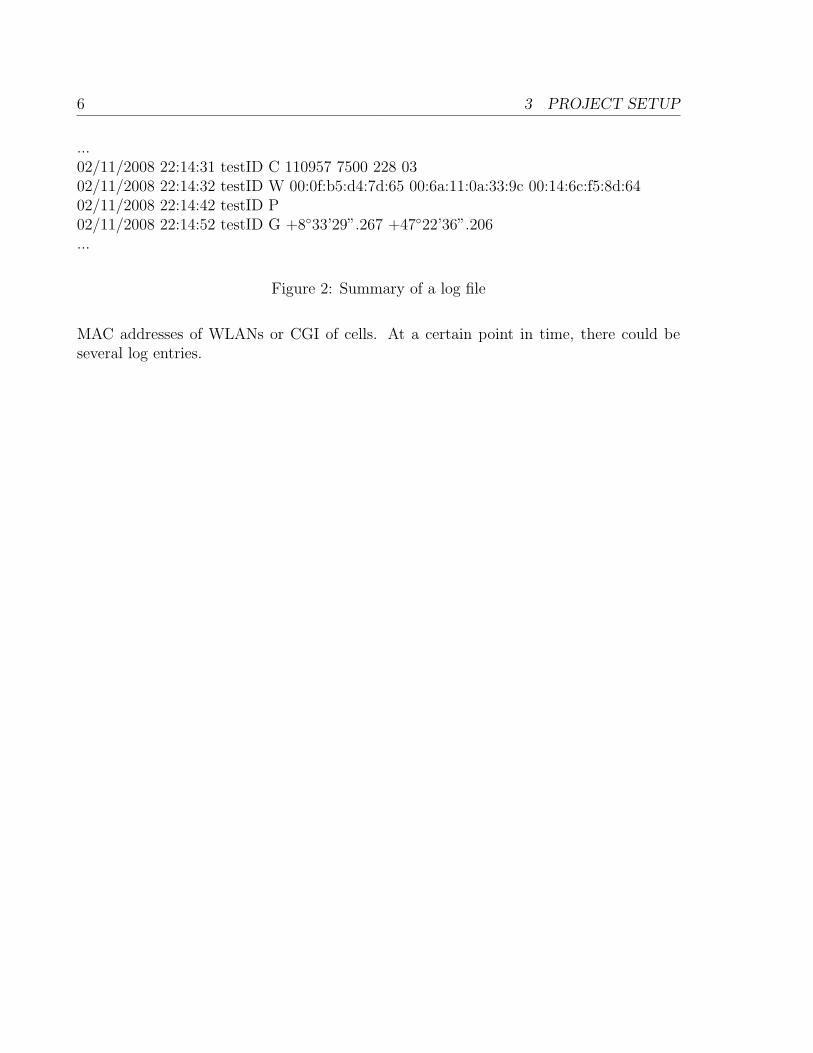
Each log entry consists of a timestamp, the userid (in this case ”testID”), a logtype iden-tifier (Ping, WLAN,GPS, Cell) and the log specific data for example GPS coordinates,

6 3 PROJECT SETUP

...02/11/2008 22:14:31 testID C 110957 7500 228 0302/11/2008 22:14:32 testID W 00:0f:b5:d4:7d:65 00:6a:11:0a:33:9c 00:14:6c:f5:8d:6402/11/2008 22:14:42 testID P02/11/2008 22:14:52 testID G +8◦33’29”.267 +47◦22’36”.206...

Figure 2: Summary of a log file

MAC addresses of WLANs or CGI of cells. At a certain point in time, there could beseveral log entries.

7

4 Data Sources

In this part the three data sources of the data logger are discussed in a short manner.There is no rigorous discussion about the technology itself since these issues are coveredin other literature.

4.1 Wireless Local Area Network

4.1.1 Identification

Each WLAN has a globally unique identifier called MAC address2. The usual notationis in form of 6 hex values in the range 0x00-0xff, spread by a colon. Fortunately, it doesnot matter whether a WLAN base station has some access restrictions. The WLAN isdetected, as long as it broadcasts beacons. A WLAN occurrence is always in conjunctionwith the detection of a MAC address.

4.1.2 Notation

In order to describe a set of MAC addresses by their occurrences, the following notationis introduced. The time instance tn denotes the start of an interval of 10s. Therefore itholds tn − tn−1 = 10sec ∀n.

mac1mac2

t0 t1 t2

Figure 3: Notation

A =

(1 0 11 1 1

)Figure 3 shows two different MAC addresses on the ordinate. If a certain MAC addresswas seen at a time instant, the square is filled in gray. In our example the mac1 was seenat the time instances t0 and t2 and mac2 at the time instances t0, t1 and t2. This notationwas also used to implement the algorithms for motion detection. A occurrences matrixwith the same design was introduced. Every element in the matrix A is either 0 or 1,where 0 denotes the absence and 1 the occurrence of a WLAN.

2There are devices which allow changing their MAC address.

8 4 DATA SOURCES

4.1.3 Availability

With the emergence of broadband internet access, the private use of WLAN became verypopular. Therefore many households have their own WLAN base station which replacesthe router and switches. This makes it very suitable for detecting a user’s position. Thedensity of public WLAN access points is very dependent on the location. In a city thereare many more public access points than in rural areas.

4.1.4 Precision

As the range of a WLAN access point heavily depends on the surroundings, it is notpossible to make a general statement about it. But in comparison to GSM, WLAN is muchmore fine-meshed and therefore allows a more precise location estimation. Measurementsin Figure 13.1 show that 80 % of the logged WLANs have a range of 60 - 240 meters. Therange is the maximum distance between two GPS coordinates where the same WLAN wasseen.

4.1.5 Remarks

A WLAN provides very precious information concerning the location detection of a userbecause the range is limited and can directly map the user to his/her location.

4.2 GSM

4.2.1 Identification

Every GSM antenna is identified by the CGI (Cell Global Identity). The CGI consists offour parts:

• MCC: Mobile Country Code (MCC = 228 for Switzerland)

• MNC: Mobile Network Code (identifies the network operator)

• LAC: Location Area Code

• CI: Cell identifier

More information about the CGI is found in the semester thesis by Fabio Magagna [1, p.17].

4.2 GSM 9

cgi1cgi2

t0 t1 t2

Figure 4: Notation

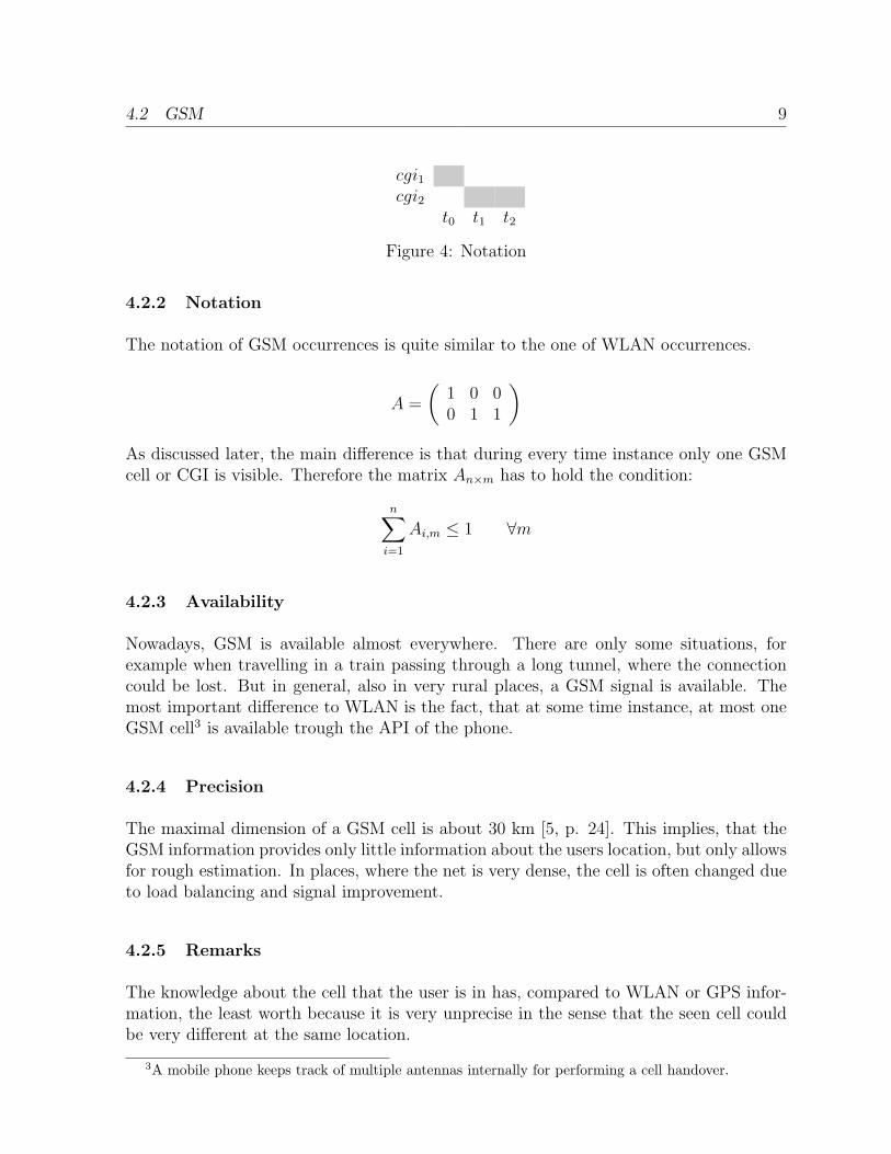
4.2.2 Notation

The notation of GSM occurrences is quite similar to the one of WLAN occurrences.

A =

(1 0 00 1 1

)As discussed later, the main difference is that during every time instance only one GSMcell or CGI is visible. Therefore the matrix An×m has to hold the condition:

n∑i=1

Ai,m ≤ 1 ∀m

4.2.3 Availability

Nowadays, GSM is available almost everywhere. There are only some situations, forexample when travelling in a train passing through a long tunnel, where the connectioncould be lost. But in general, also in very rural places, a GSM signal is available. Themost important difference to WLAN is the fact, that at some time instance, at most oneGSM cell3 is available trough the API of the phone.

4.2.4 Precision

The maximal dimension of a GSM cell is about 30 km [5, p. 24]. This implies, that theGSM information provides only little information about the users location, but only allowsfor rough estimation. In places, where the net is very dense, the cell is often changed dueto load balancing and signal improvement.

4.2.5 Remarks

The knowledge about the cell that the user is in has, compared to WLAN or GPS infor-mation, the least worth because it is very unprecise in the sense that the seen cell couldbe very different at the same location.

3A mobile phone keeps track of multiple antennas internally for performing a cell handover.

10 4 DATA SOURCES

4.3 GPS

The global positioning system provides very precise information about the location andthe speed of an object. A GPS device receives the exact position and timestamp frommultiple satellites (at least four) which enables it to calculate the exact position of anobject.

4.3.1 Identification

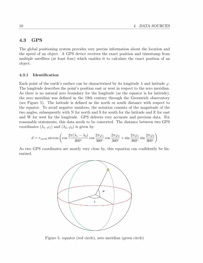
Each point of the earth’s surface can be characterized by its longitude λ and latitude ϕ.The longitude describes the point’s position east or west in respect to the zero meridian.As there is no natural zero boundary for the longitude (as the equator is for latitude),the zero meridian was defined in the 19th century through the Greenwich observatory(see Figure 5). The latitude is defined as the north or south distance with respect tothe equator. To avoid negative numbers, the notation consists of the magnitude of thetwo angles, subsequently with N for north and S for south for the latitude and E for eastand W for west for the longitude. GPS delivers very accurate and precious data. Forreasonable statements, this data needs to be converted. The distance between two GPScoordinates (λ1, ϕ1) and (λ2, ϕ2) is given by:

d = rearth arccos

(cos

2π(λ1 − λ2)

360◦cos

2πϕ1

360◦cos

2πϕ2

360◦+ sin

2πϕ1

360◦sin

2πϕ2

360◦

)As two GPS coordinates are mostly very close by, this equation can confidently be lin-earized.

Figure 5: equator (red circle), zero meridian (green circle)

4.4 NOTATION 11

4.3.2 Availability

In general, GPS is freely available worldwide. But in this context, the term availabilitybetter covers the fact, that the GPS reception is mostly only possible outdoors. There arerare situations where a GPS signal can be received indoors. But in general, the receptionis ideal within a clear line of sight to the sky.

4.3.3 Precision

GPS has a accuracy of a few meters [3]. Our practical experience however, shows thatthis accuracy is achieved only in the best case. It mainly depends on the speed of theusers movement and the actual number of satellites receiving information. Sometimes theeffective location is up to 100 m away from the GPS measurement.

4.3.4 Remarks

A GPS measuring point is in this context the most valuable data. It provides preciseknowledge about the user’s location without further knowledge or data processing. Havingseveral of them allows for a very accurate distance and speed calculation.

4.4 Notation

4.4.1 Definition of the Measuring Point

A measuring point is defined by one piece of information consisting of a WLAN MACaddress, a GSM cell CGI or coordinates from GPS. It always has a timestamp and acorrelating userid, which maps the information to a specific user.

4.4.2 Definition of Estimation

Both location and movement estimation are done by analyzing an interval of 5 minutes.Logging every 10 seconds, we potentially have 30 time instances with one or more measur-ing points. This is a key parameter of the system. Making the interval too long, decreasesthe resolution of the estimation. Reducing the interval makes an estimation of movementhard.

12 5 DATA VISUALIZATION

5 Data Visualization

5.1 Web Frontend

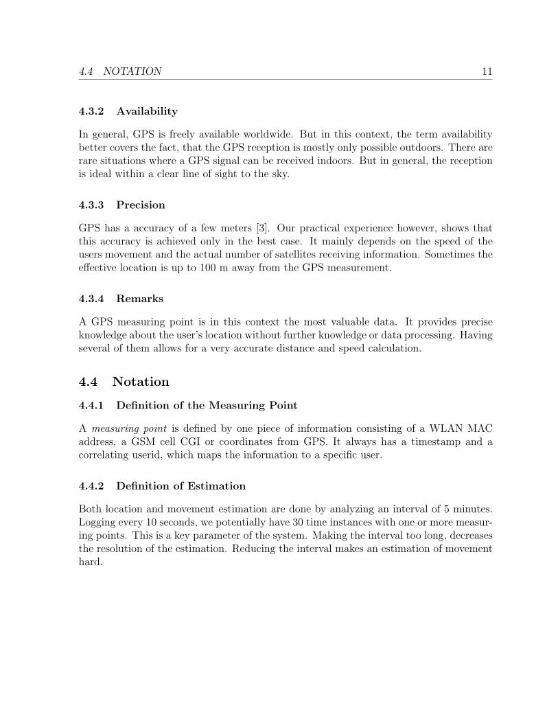
To visualize the measured data, a web frontend was implemented. It has many advantagesover images, because Javascript adds a lot of features for direct interaction. Figure 6 showsa screenshot of the site. The red, green and blue dots denote the occurrences of somemeasuring points. For convenience, they are ordered by their first occurrence. All of thesepoints provide additional information when one hovers over them with the mouse. Theabscissa represents the time evolving in 1 minute steps indicated by the distance betweentwo black bars. For each time instance (interval of 10 seconds) the ordinate depicts themeasuring point seen at this time. The points among the time line depict the locationand movement estimations.

Figure 6: data visualization in a web browser

The header of the diagram 1) shows the weekday and the exact start and end of thevisualized data. The green dots 2) depict WLAN occurrences, where the red ones 3)show the seen GSM cell for each time instance . The blue dots 4) indicate, that there are

5.2 MANUAL DATA COLLECTION 13

available GPS measurements. As mentioned above, the black bars 5) indicate the timein one minute steps. The yellow dot 6) provides information about the location whenhovered by the mouse. 7) denotes the movement type (if any), which was found in thejournal. 8),9),10) are the suggestions from three different movement detection algorithms(the symbols denote classes), while 11) provides functionality for training the SVM.

5.2 Manual Data Collection

For later use it is very important to have reference data depicted by some time intervalswhere a location and/or movement is/are defined. This data is important for the laterevaluation of the algorithm’s performances. For training the classifier the web frontendin Figure 6 is used. Such a training-vector only consist of a timestamp and the kind ofmovement (standing, walking, moving by train, moving by car). The journal used for theperformance analysis always consist of a timestamp, a location and/or a movement type.This data is collected using a simple website.

14 6 DATA GATHERING

6 Data Gathering

This part discusses some data structures, which could be derived from the log data inorder to approximate the users location or movement. Because many of these algorithmstake a lot of time to be computed, they are computed in a daily batch mode.

6.1 GSM,WLAN Positions

When GPS coordinates are available the locations of WLAN and GSM can be estimated.If there are multiple coordinates available for a cell or WLAN, the known coordinatesare averaged. The estimation accuracy grows with the number of measuring points. Thisrough position estimation could then be used for determining the user’s environment.

6.2 WLAN Connectivity Graph

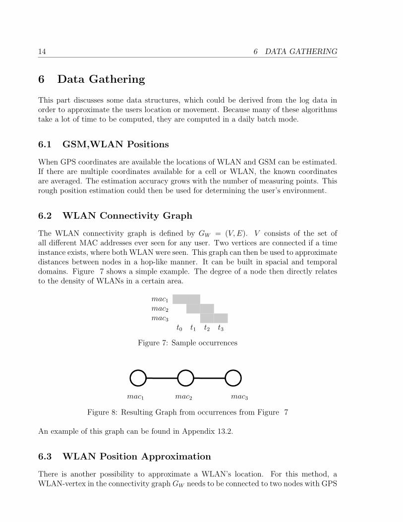
The WLAN connectivity graph is defined by GW = (V,E). V consists of the set ofall different MAC addresses ever seen for any user. Two vertices are connected if a timeinstance exists, where both WLAN were seen. This graph can then be used to approximatedistances between nodes in a hop-like manner. It can be built in spacial and temporaldomains. Figure 7 shows a simple example. The degree of a node then directly relatesto the density of WLANs in a certain area.

mac1mac2mac3

t0 t1 t2 t3

Figure 7: Sample occurrences

mac1 mac2 mac3

Figure 8: Resulting Graph from occurrences from Figure 7

An example of this graph can be found in Appendix 13.2.

6.3 WLAN Position Approximation

There is another possibility to approximate a WLAN’s location. For this method, aWLAN-vertex in the connectivity graph GW needs to be connected to two nodes with GPS

6.3 WLAN POSITION APPROXIMATION 15

information. This approximation is rather imprecise but allows a rough approximationof the WLANs location. Like before, the coordinates of the two outer WLANs are justaveraged.

16 7 LOCATION ESTIMATION

7 Location Estimation

The preceding Abakabar application already had a location estimation feature. It allowedadding personal places, which then were recognized. But the system was not able tocapture structures for example having different rooms in one building.

7.1 Definition of Location

In our context, a location is a hierarchically defined and categorized place of a certaindimension. Each location has a parent location. The root of this tree is the world. Alllocations are arranged in categories. These categories are sorted by size and are definedby:

• Country

• Region

• Village

• Area

• Building

• Room

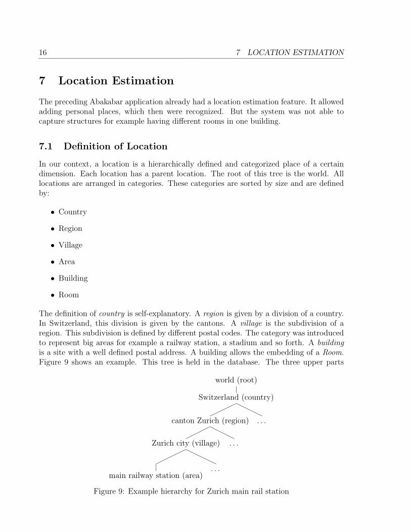
The definition of country is self-explanatory. A region is given by a division of a country.In Switzerland, this division is given by the cantons. A village is the subdivision of aregion. This subdivision is defined by different postal codes. The category was introducedto represent big areas for example a railway station, a stadium and so forth. A buildingis a site with a well defined postal address. A building allows the embedding of a Room.Figure 9 shows an example. This tree is held in the database. The three upper parts

world (root)

Switzerland (country)

canton Zurich (region)

Zurich city (village)

main railway station (area). . .

. . .

. . .

Figure 9: Example hierarchy for Zurich main rail station

7.2 LOCATION ACQUISITION 17

(Country,Region, Village) are up to now hand maintained. By using third party providers,the handling of the tree could be automated by coming up with suggestions for locations.

7.2 Location Acquisition

The locations are learned from the user’s input. The user can decide if a location is public(for example a railway station) or if it is private (for example his/her accomodation). Newplaces can be added online over the mobile device. If a place is tagged as location, allthe concerning log information is stored as characteristical for that place. For places withdimensions larger than the range of a WLAN, the data of the WLAN connectivity graph(see section 6.2) is taken into account. This means that WLANs which are 1 hop (forbuildings) or 2 hops (for areas) away are taken into the set of characteristical WLANs.Up to now only the leaves of the tree are taken into account for location estimation.

7.3 Implementation

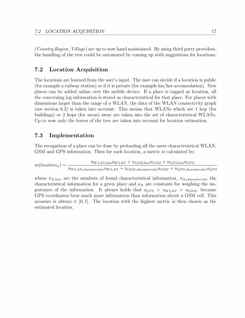
The recognition of a place can be done by preloading all the users characteristical WLAN,GSM and GPS information. Then for each location, a metric is calculated by:

m(locationn) =nWLAN,hitsaWLAN + nGSM,hitsaGSM + nGPS,hitsaGPS

nWLAN,characteristicaWLAN + nGSM,characteristicaGSM + nGPS,characteristicaGPS

where nX,hits are the numbers of found characteristical information, nX,characteristic thecharacteristical information for a given place and aX are constants for weighing the im-portance of the information. It always holds that aGPS > aWLAN > aGSM , becauseGPS coordinates bear much more information than information about a GSM cell. Thismeasure is always ∈ [0, 1]. The location with the highest metric is then chosen as theestimated location.

18 8 MOVEMENT ESTIMATION

8 Movement Estimation

One main goal of the project is to make statements about the user’s movement. As far aspossible, these statements should not base upon third party imported data4. The possiblekinds of movements (later called classes) were refined to:

• standing (c = 1)

• walking (c = 2)

• moving by car (c = 3)

• moving by train (c = 4)

Each of these classes has its characteristics. Standing for example, can be detected veryeasily just by looking for a WLAN that appeared constantly over a given time. This alsomeans that statements about standing are pretty reliable, because there is no ambiguity.Walking or moving in general is more complicated, because different kinds of movementlead to similar patterns. Having GPS data is very helpful because the exact speed andplace where somebody is going is known.

8.1 Movement Measurements by GPS

This is the only part of the project which uses data from a third party provider tomake a statement about the user’s movement. It is further important that the followingalgorithm is only applicable if the exact position of a user is known, which means thatGPS is available over a certain period. The idea is to check the users position against amap to determine whether the user moves by train or by car. The data is provided byopenstreetmap [7], which is a free-to-use map provider and the information is availablefor the whole world. For performance reasons, only the data of the Swiss railsystem wasused.

8.1.1 Map Data Format

Both streets and railroads are given by subsequent points in form of GPS coordinates.This means that every subsequent pair of points forms a vector.

8.1.2 Distance to Railroads and Streets

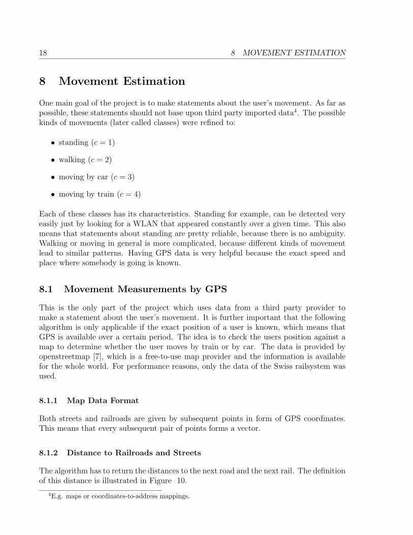
The algorithm has to return the distances to the next road and the next rail. The definitionof this distance is illustrated in Figure 10.

4E.g. maps or coordinates-to-address mappings.

8.1 MOVEMENT MEASUREMENTS BY GPS 19

Figure 10: The striped spots are the known locations of a railroad or street, where thedotted ones identify GPS measurements.

If the point lies within the perpendicular boundaries of two railroad/street-points, thedistance is defined by the perpendicular distance. If this point lies outside these bound-aries, the distance is given by the shortest gap to a railroad/street-point. Figure 11 showsthe distance to railsroad/street in details.

The vector pointing from (x1, y1) to (x2, y2) is given by

~r12 =

(x2 − x1

y2 − y1

)The vector from (x1, y1) to (x0, y0) is represented as

~r1 =

(x0 − x1

y0 − y1

)Building the vector ~p which is perpendicular to ~r12 can be retrieved by rotating ~r12 by 90degrees:

~p =

(cosα − sinαsinα cosα

)~r12 =

(y1 − y2

x2 − x1

)for α = π

2. The distance d is now given by the length of the projection of ~r1 onto ~p:

drail,road =~r1 · ~p|~p|

=|(x0 − x1)(y1 − y2) + (y0 − y1)(x2 − x1)|√

(x2 − x1)2 + (y1 − y2)2

20 8 MOVEMENT ESTIMATION

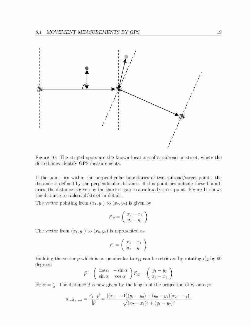
Figure 11: Detailed view

To detect if the point is lying inside the defined perpendicular boundaries the point hasto fulfill the following inequation:

sgn(~r12 · ~r1) 6= sgn(~r12 · ~r2)

This means, that the scalar products onto the vector ~r12 have different signs. If thisinequation is not fulfilled, one just take the distance to the nearest railroad/street point.

8.1.3 Speed Estimation

Having n logs in a given time interval with GPS coordinates, the average speed can becalculated as:

vGPS =1

n− 1

n−2∑i=0

d(λi+1, λi, ϕi+1, ϕi)

∆t(i+ 1, i)

8.2 Movement Metrics by WLAN

This part describes an approach for speed estimation using only WLAN occurrences. Themain problem is that there is no a-priori knowledge about the WLAN densities.

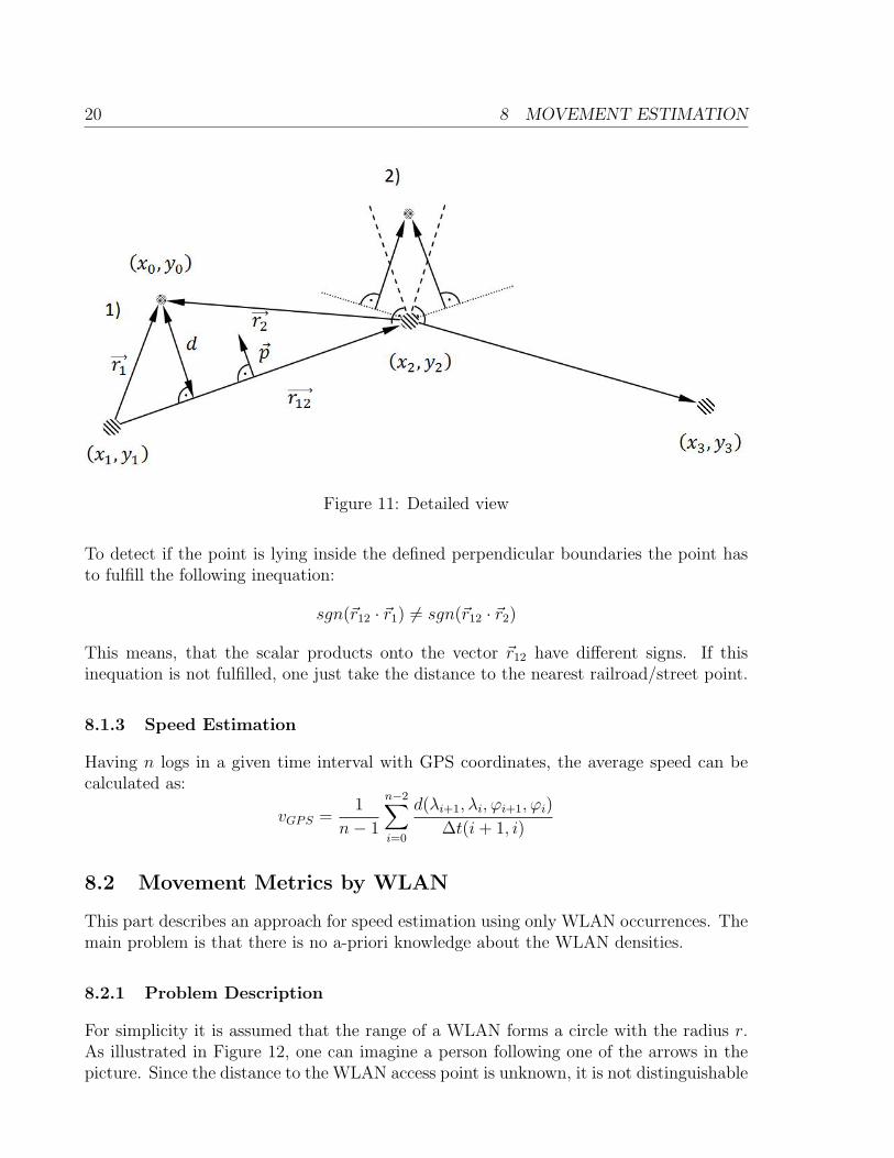
8.2.1 Problem Description

For simplicity it is assumed that the range of a WLAN forms a circle with the radius r.As illustrated in Figure 12, one can imagine a person following one of the arrows in thepicture. Since the distance to the WLAN access point is unknown, it is not distinguishable

8.2 MOVEMENT METRICS BY WLAN 21

which arrow (1 or 2) the user is following. The only thing that is measurable is the timeduration during which the WLAN was seen.

Figure 12: WLAN access point indicated by the cross

8.2.2 Approximation

Introducing the random variable D ∼ U(0, r) which expresses the perpendicular distanceto the WLAN passing through the range, and defining the random variable L as the lengthof seeing the WLAN crossing the range and is given by:(

L

2

)2

+D2 = r2

L = 2√r2 −D2

E[L] = 2E[√r2 −D2] =

∫ r

0

2

r

√r2 − x2dx =

rπ

2

This leads to the conclusion that in average a WLAN is seen in rπ2

of its length. So, atleast in average, the speed can be stated as:

vapprox =rπ

2tWLAN

(1)

where tWLAN can be extracted directly out of the logs, and r is a statistically revealedconstant. As seen later, it suffices to take tWLAN into account for movement recognition.The assumption that the reception area of a WLAN is a circle is very naive. Even in freespace the directional characteristic of the antenna would not be spheric. But to keep thecalculations simple, the circle is always the easiest choice. Also the choice of the randomvariable D is held as simple as possible.

22 8 MOVEMENT ESTIMATION

8.2.3 Practical Implementation

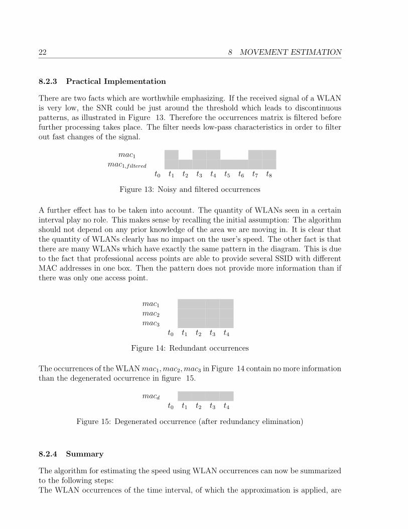
There are two facts which are worthwhile emphasizing. If the received signal of a WLANis very low, the SNR could be just around the threshold which leads to discontinuouspatterns, as illustrated in Figure 13. Therefore the occurrences matrix is filtered beforefurther processing takes place. The filter needs low-pass characteristics in order to filterout fast changes of the signal.

mac1mac1,filtered

t0 t1 t2 t3 t4 t5 t6 t7 t8

Figure 13: Noisy and filtered occurrences

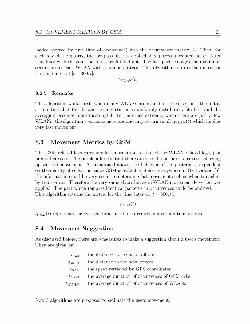
A further effect has to be taken into account. The quantity of WLANs seen in a certaininterval play no role. This makes sense by recalling the initial assumption: The algorithmshould not depend on any prior knowledge of the area we are moving in. It is clear thatthe quantity of WLANs clearly has no impact on the user’s speed. The other fact is thatthere are many WLANs which have exactly the same pattern in the diagram. This is dueto the fact that professional access points are able to provide several SSID with differentMAC addresses in one box. Then the pattern does not provide more information than ifthere was only one access point.

mac1mac2mac3

t0 t1 t2 t3 t4

Figure 14: Redundant occurrences

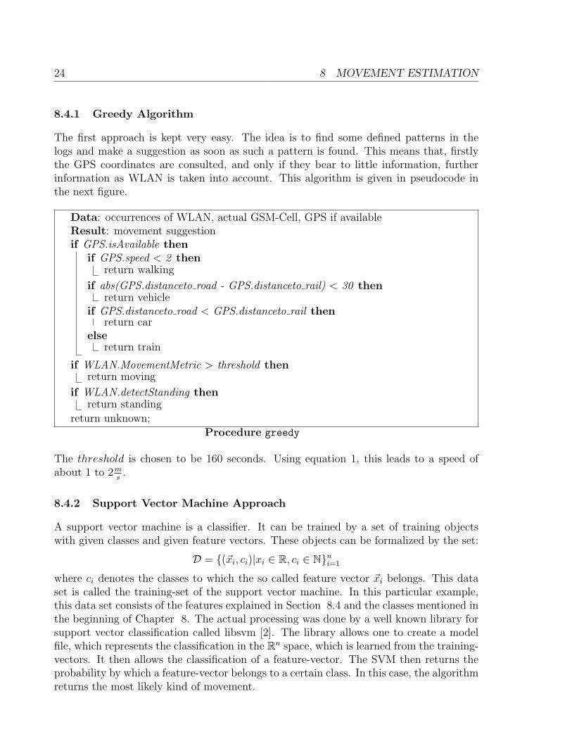
The occurrences of the WLANmac1,mac2,mac3 in Figure 14 contain no more informationthan the degenerated occurrence in figure 15.

macdt0 t1 t2 t3 t4

Figure 15: Degenerated occurrence (after redundancy elimination)

8.2.4 Summary

The algorithm for estimating the speed using WLAN occurrences can now be summarizedto the following steps:The WLAN occurrences of the time interval, of which the approximation is applied, are

8.3 MOVEMENT METRICS BY GSM 23

loaded (sorted by first time of occurrence) into the occurrences matrix A. Then, foreach row of the matrix, the low-pass filter is applied to suppress unwanted noise. Afterthat lines with the same patterns are filtered out. The last part averages the maximumoccurrence of each WLAN with a unique pattern. This algorithm returns the metric forthe time interval [t− 300, t]:

tWLAN(t)

8.2.5 Remarks

This algorithm works best, when many WLANs are available. Because then, the initialassumption that the distance to any station is uniformly distributed, fits best and theaveraging becomes more meaningful. In the other extreme, when there are just a fewWLANs, the algorithm’s variance increases and may return small tWLAN(t) which impliesvery fast movement.

8.3 Movement Metrics by GSM

The GSM related logs carry similar information to that of the WLAN related logs, justin another scale. The problem here is that there are very discontinuous patterns showingup without movement. As mentioned above, the behavior of the patterns is dependenton the density of cells. But since GSM is available almost everywhere in Switzerland [5],the information could be very useful to determine fast movement such as when traviellngby train or car. Therefore the very same algorithm as in WLAN movement detection wasapplied. The part which removes identical patterns in occurrences could be omitted.This algorithm returns the metric for the time interval [t− 300, t]:

tGSM(t)

tGSM(t) represents the average duration of occurrences in a certain time interval.

8.4 Movement Suggestion

As discussed before, there are 5 measures to make a suggestion about a user’s movement.They are given by:

drail the distance to the next railroads

dstreet the distance to the next streets

vGPS the speed retrieved by GPS coordinates

tGSM the average duration of occurrences of GSM cells

tWLAN the average duration of occurrences of WLANs

Now 3 algorithms are proposed to estimate the users movement.

24 8 MOVEMENT ESTIMATION

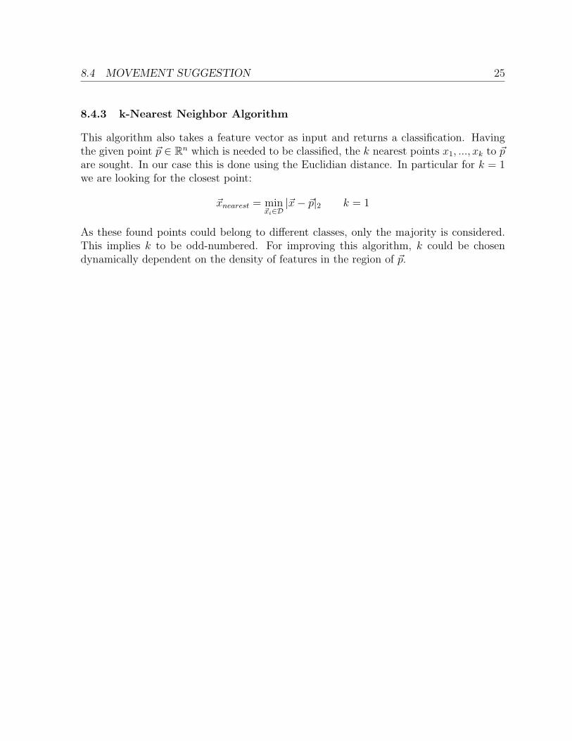
8.4.1 Greedy Algorithm

The first approach is kept very easy. The idea is to find some defined patterns in thelogs and make a suggestion as soon as such a pattern is found. This means that, firstlythe GPS coordinates are consulted, and only if they bear to little information, furtherinformation as WLAN is taken into account. This algorithm is given in pseudocode inthe next figure.

Data: occurrences of WLAN, actual GSM-Cell, GPS if availableResult: movement suggestionif GPS.isAvailable then

if GPS.speed < 2 thenreturn walking

if abs(GPS.distanceto road - GPS.distanceto rail) < 30 thenreturn vehicle

if GPS.distanceto road < GPS.distanceto rail thenreturn car

elsereturn train

if WLAN.MovementMetric > threshold thenreturn moving

if WLAN.detectStanding thenreturn standing

return unknown;

Procedure greedy

The threshold is chosen to be 160 seconds. Using equation 1, this leads to a speed ofabout 1 to 2m

s.

8.4.2 Support Vector Machine Approach

A support vector machine is a classifier. It can be trained by a set of training objectswith given classes and given feature vectors. These objects can be formalized by the set:

D = {(~xi, ci)|xi ∈ R, ci ∈ N}ni=1

where ci denotes the classes to which the so called feature vector ~xi belongs. This dataset is called the training-set of the support vector machine. In this particular example,this data set consists of the features explained in Section 8.4 and the classes mentioned inthe beginning of Chapter 8. The actual processing was done by a well known library forsupport vector classification called libsvm [2]. The library allows one to create a modelfile, which represents the classification in the Rn space, which is learned from the training-vectors. It then allows the classification of a feature-vector. The SVM then returns theprobability by which a feature-vector belongs to a certain class. In this case, the algorithmreturns the most likely kind of movement.

8.4 MOVEMENT SUGGESTION 25

8.4.3 k-Nearest Neighbor Algorithm

This algorithm also takes a feature vector as input and returns a classification. Havingthe given point ~p ∈ Rn which is needed to be classified, the k nearest points x1, ..., xk to ~pare sought. In our case this is done using the Euclidian distance. In particular for k = 1we are looking for the closest point:

~xnearest = min~xi∈D|~x− ~p|2 k = 1

As these found points could belong to different classes, only the majority is considered.This implies k to be odd-numbered. For improving this algorithm, k could be chosendynamically dependent on the density of features in the region of ~p.

26 9 PERFORMANCE ANALYSIS

9 Performance Analysis

To make clear statements about the algorithm’s performance, a test bench was needed.To do that a journal had to be kept by hand. This data is then fed into the databasefor later evaluation of the three algorithms. An entry in the journal consist of the timeand of the place or the movement. The time span for which the diary is available is theniterated and compared against the movement estimations of the three algorithms and thelocation estimation.

9.1 Location Estimation Analysis

The location estimation lead to a accuracy of about 87%. This means that 87% of thetime the estimation matched the given location in the journal. As the test bench was putinto context, where most of the locations were tagged this value is not a surprise. Thisvalue shows that if user depending locations are tagged, they are recognized.

9.2 Movement Estimation Analysis

9.2.1 Notation

Later used percentages called precision and recall are defined by:

Precision =tp

tp+ fp∈ [0, 1]

Recall =tp

tp+ fn∈ [0, 1]

The number tp (true-positive) depicts the items correctly labeled as belonging to the class(the journal entry corresponds to the estimation of the algorith). fp (false-positive) is thenumber wronlgy classified as belonging to a class (altough it does not belong to) and fn(false-negative) is the count of items not labeled as belonging to a class altough it doesbelong to. [8]

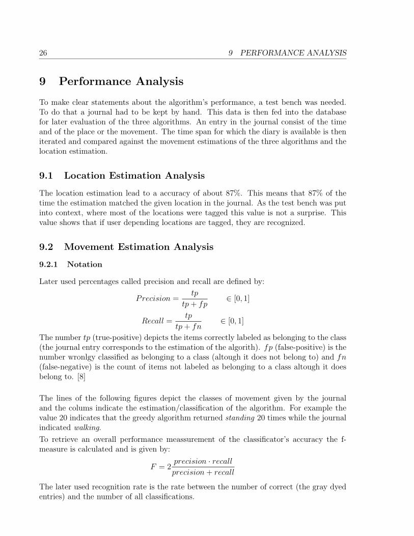
The lines of the following figures depict the classes of movement given by the journaland the colums indicate the estimation/classification of the algorithm. For example thevalue 20 indicates that the greedy algorithm returned standing 20 times while the journalindicated walking.

To retrieve an overall performance meassurement of the classificator’s accuracy the f-measure is calculated and is given by:

F = 2precision · recallprecision+ recall

The later used recognition rate is the rate between the number of correct (the gray dyedentries) and the number of all classifications.

9.2 MOVEMENT ESTIMATION ANALYSIS 27

9.2.2 Greedy Algorithm

unknown standing walking car train precisionstanding 2 244 16 1 0 93%walking 14 20 32 0 0 48%car 0 0 2 9 0 82%train 1 1 2 1 8 62%recall 92% 62% 82% 100%

Figure 16: performance of the Greedy Algorithm

average precision 71 %average recall 84 %F-measure 77 %recognition rate 82 %

Figure 17: overall performance of the Greedy Algorithm

The greedy algorithm shows good performance detecting standing, moving by train andmoving by car. Especially the last two classes are detected very reliable because thealgorithm never will propose these two classes without having some GPS informations.Also in estimating standing it shows high precision and recall. This is not a surprisebecause standing is the easiest recognizable class. The main weakness of the algorithm isfound in estimating the class walking. This comes from the fact that the decision betweenwalking and standing is mostly5 done by analyzing the WLAN occurrences. The reasonfor clasify standing wrongly as walking comes from the fact that at some locations certainWLANs are visible very sporadicly.The reason why the greedy algorithms performs better than the other two algorithmsdestinguishing between train and car is due the fact that the greedy algorithm has a returnvalue vehicle. If this estmation shows up the software decides for the given movement inthe journal.

9.2.3 Support Vector Machine Classification

As expected, also the support vector machine approach shows good performance in de-tecting standing. The reason for this is the fact that standing is specified only by onefeature-vector6 which is very different (in a Eucledian distance manner) to feature-vectorsof other classes.The classification of walking is in comparison to the greedy algorithm better because theSVM approach does not depend on a given threshold and also takes GSM informationinto account.

5Because no GPS data is available.6All WLAN and GSM cells were see all the time and the GPS data indicates no movement

28 9 PERFORMANCE ANALYSIS

standing walking car train precisionstanding 226 35 2 0 86%walking 5 60 0 1 91%car 0 1 8 2 73%train 0 3 4 6 46%recall 98% 61% 57% 67%

Figure 18: performance of the Support Vector Machine Classification

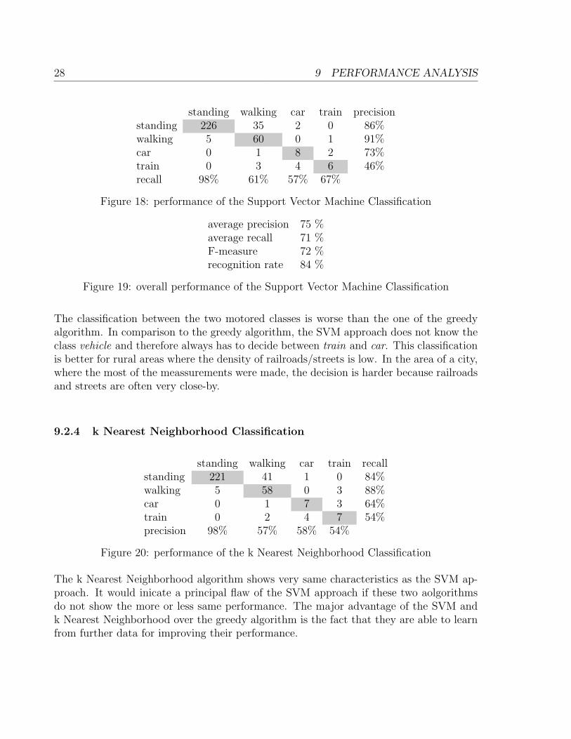
average precision 75 %average recall 71 %F-measure 72 %recognition rate 84 %

Figure 19: overall performance of the Support Vector Machine Classification

The classification between the two motored classes is worse than the one of the greedyalgorithm. In comparison to the greedy algorithm, the SVM approach does not know theclass vehicle and therefore always has to decide between train and car. This classificationis better for rural areas where the density of railroads/streets is low. In the area of a city,where the most of the meassurements were made, the decision is harder because railroadsand streets are often very close-by.

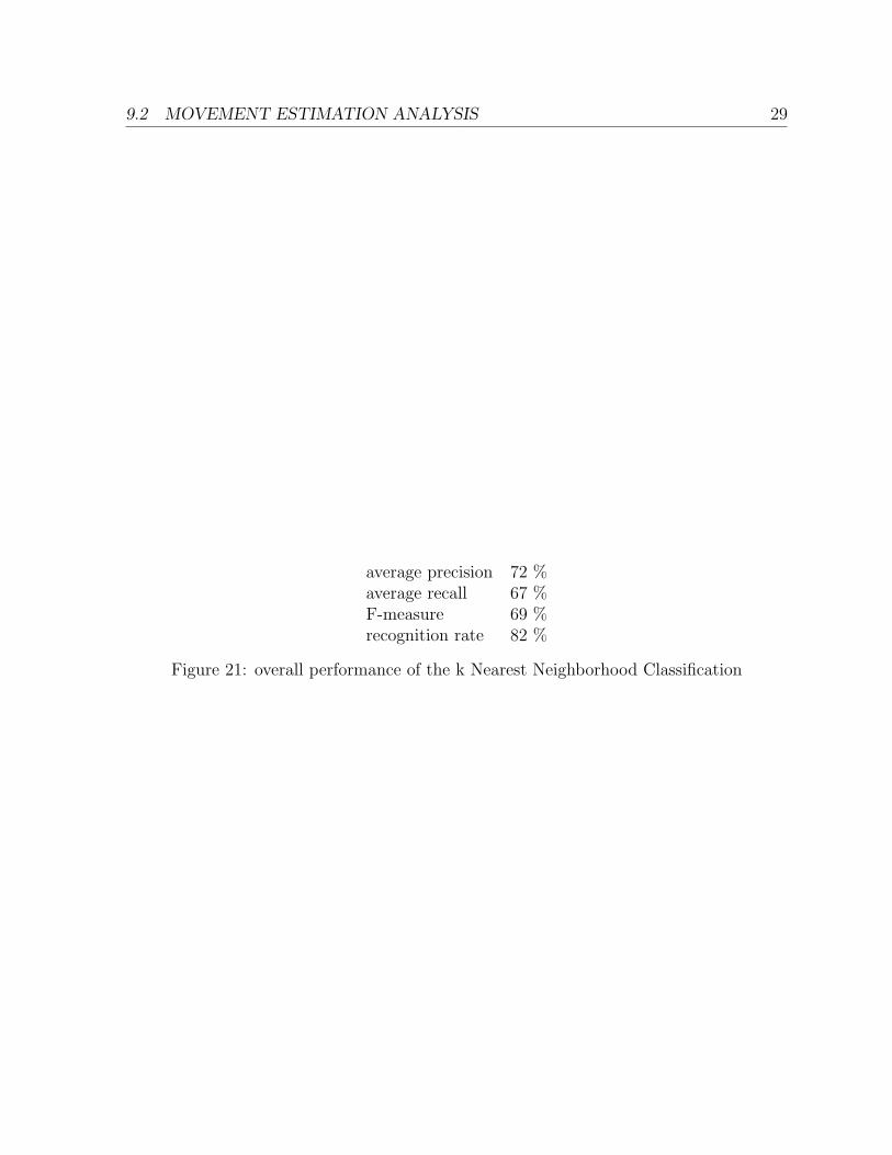
9.2.4 k Nearest Neighborhood Classification

standing walking car train recallstanding 221 41 1 0 84%walking 5 58 0 3 88%car 0 1 7 3 64%train 0 2 4 7 54%precision 98% 57% 58% 54%

Figure 20: performance of the k Nearest Neighborhood Classification

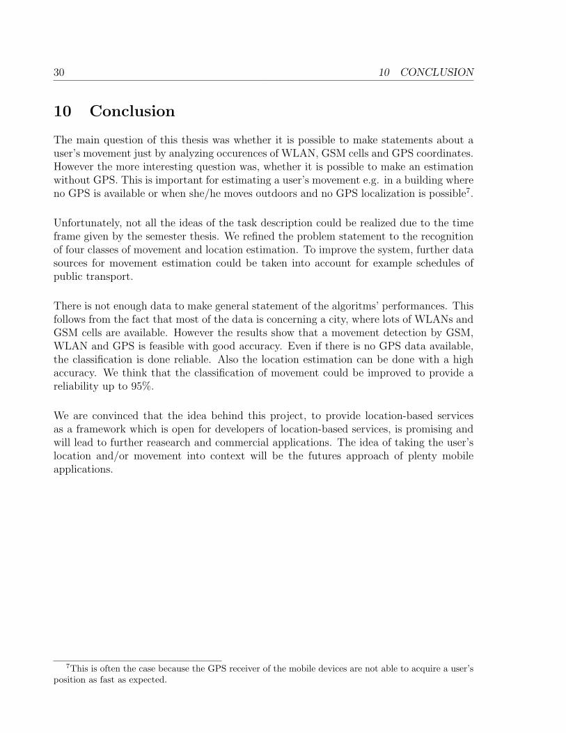
The k Nearest Neighborhood algorithm shows very same characteristics as the SVM ap-proach. It would inicate a principal flaw of the SVM approach if these two aolgorithmsdo not show the more or less same performance. The major advantage of the SVM andk Nearest Neighborhood over the greedy algorithm is the fact that they are able to learnfrom further data for improving their performance.

9.2 MOVEMENT ESTIMATION ANALYSIS 29

average precision 72 %average recall 67 %F-measure 69 %recognition rate 82 %

Figure 21: overall performance of the k Nearest Neighborhood Classification

30 10 CONCLUSION

10 Conclusion

The main question of this thesis was whether it is possible to make statements about auser’s movement just by analyzing occurences of WLAN, GSM cells and GPS coordinates.However the more interesting question was, whether it is possible to make an estimationwithout GPS. This is important for estimating a user’s movement e.g. in a building whereno GPS is available or when she/he moves outdoors and no GPS localization is possible7.

Unfortunately, not all the ideas of the task description could be realized due to the timeframe given by the semester thesis. We refined the problem statement to the recognitionof four classes of movement and location estimation. To improve the system, further datasources for movement estimation could be taken into account for example schedules ofpublic transport.

There is not enough data to make general statement of the algoritms’ performances. Thisfollows from the fact that most of the data is concerning a city, where lots of WLANs andGSM cells are available. However the results show that a movement detection by GSM,WLAN and GPS is feasible with good accuracy. Even if there is no GPS data available,the classification is done reliable. Also the location estimation can be done with a highaccuracy. We think that the classification of movement could be improved to provide areliability up to 95%.

We are convinced that the idea behind this project, to provide location-based servicesas a framework which is open for developers of location-based services, is promising andwill lead to further reasearch and commercial applications. The idea of taking the user’slocation and/or movement into context will be the futures approach of plenty mobileapplications.

7This is often the case because the GPS receiver of the mobile devices are not able to acquire a user’sposition as fast as expected.

31

11 Future Work

11.1 Massive Data Gathering

To improve the proposed algorithms for estimating the locations of WLANs and GSMcells, it is very important to have as much information as possible. Up to now, thereare only a bit more than 2 weeks of logs concerning only one user. The available data issufficient to implement algorithms but not to show the functionality of the system in alarge scale.

11.2 Mobile Application

Today’s mobile devices provide more information about their environment than used inthis project. There is a tendency to equip the mobile devices with more and more sensors,e.g. accelerometers. This enables the detection of movement from another aspect. Forexample walking up stairs, using an elevator or similar moevements. Another approach isusing the microphone to “hear” whether the user is for example moving in a train or car.These features are better implemented directly onto the mobile device but could surelyimprove the accuracy of our estimations.

11.3 Server Application

In order to provide much more information about a user’s location or movement, severalfree web services could be taken into account to improve this service. As an example,there is a commercial product which provides a coordinates-to-address mapping. Thiscould be used to provide proposals to the user’s location for easier tagging of a place. Toimprove the movement detection, one could try to directly map a train ride to the actualtimetable of the trains. This could then lead to further estimations, where a user will bein future, because the system learned from the past, that the user left a train at a certainstation at a certain time and weekday.

11.4 Improvement of the Classification Algorithms

The support vector machine and the k Nearest Neighborhood Algorithms could be ex-tended with more features. Further features could be the maximal and minimal velocityover a certain period of time to distinguish more precisely between walking and driving acar that is stuck in traffic.A further approach is to take into account more than five minutes of a user’s movement.For example a period of 20-30 minutes. This allows a better detection of a fast movinguser by considering the GSM cells.

32 12 ACKNOWLEDGMENTS

12 Acknowledgments

I would like to thank my advisor, Michael Kuhn, whose knowledge and patience addedconsiderably to my semester thesis. A special thanks goes to Fabio Magagna, who sup-ported me during the thesis and shared his experience with me.

REFERENCES 33

References

[1] Semester Thesis of Fabio Magagna

[2] LibSVM – A library for Support Vector Machines

[3] Erreichbare Genauigkeit bei GPS-Positionsbestimungen

[4] Eigenbehaviors: Identifying Structure in Routine

[5] Ad Hoc and Sensor Networks, Chapter 14, Mobility

[6] Magizne ’explore’, p. 18

[7] Openstreetmap

[8] Precision and recall - Wikipedia, the free encyclopedia

[9] Berg Insight. Strategic analysis of the European mobile LBS market. Berg InsightBRG1352742, 2006

[10] Sensing the World with Mobile Devices

[11] Apple - iPhone - App Store und Programme fur das iPhone

34 13 APPENDIX

13 Appendix

13.1 WLAN Range Histogram

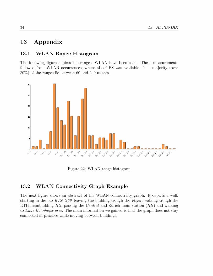
The following figure depicts the ranges, WLAN have been seen. These measurementsfollowed from WLAN occurrences, where also GPS was available. The majority (over80%) of the ranges lie between 60 and 240 meters.

Figure 22: WLAN range histogram

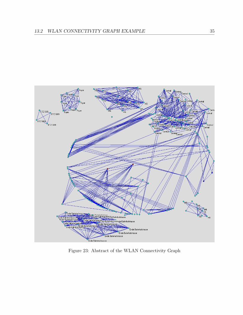
13.2 WLAN Connectivity Graph Example

The next figure shows an abstract of the WLAN connectivity graph. It depicts a walkstarting in the lab ETZ G69, leaving the building trough the Foyer, walking trough theETH mainbuilding HG, passing the Central and Zurich main station (HB) and walkingto Ende Bahnhofstrasse. The main information we gained is that the graph does not stayconnected in practice while moving between buildings.

13.2 WLAN CONNECTIVITY GRAPH EXAMPLE 35

Figure 23: Abstract of the WLAN Connectivity Graph