Self-organisation of Protein Patterns - arXiv

Self-organisation of Protein Patterns— Lecture Notes for Les Houches 2018 Summer School on“Active Matter and Nonequilibrium Statistical Physics” —

Erwin Frey∗and Fridtjof BraunsArnold Sommerfeld Center for Theoretical Physics,

Ludwig–Maximilians–Universitat Munchen,Theresienstraße 37, D-80333 Munchen, Germany

∗ [email protected]

arX

iv:2

012.

0179

7v1

[ph

ysic

s.bi

o-ph

] 3

Dec

202

0

2

Contents1 Introduction 3

2 Protein patterns 62.1 Intracellular protein patterns . . . . . . . . . . . . . . . . . . . 62.2 General biophysical principles of intracellular pattern formation 92.3 Reaction-diffusion equations in cellular geometry . . . . . . . . 11

3 Protein reaction kinetics 193.1 Rate equations for well-mixed biochemical systems . . . . . . . 193.2 One-component systems . . . . . . . . . . . . . . . . . . . . . . 213.3 General two-component systems . . . . . . . . . . . . . . . . . 35

4 Spatially extended two-component systems 474.1 Classical Turing system . . . . . . . . . . . . . . . . . . . . . . 494.2 Mass-conserving two-component reaction–diffusion systems . . 554.3 Linear stability analysis of mass-conserving systems . . . . . . 584.4 Mass-redistribution instability . . . . . . . . . . . . . . . . . . . 614.5 Stationary states, flux balance, and landmark points . . . . . . 68

5 The role of bulk-boundary coupling for membrane patterns 785.1 Elementary examples in column geometry . . . . . . . . . . . . 785.2 Linear stability analysis in box geometry . . . . . . . . . . . . . 885.3 Pattern formation without a lateral instability . . . . . . . . . . 94

6 Control space dynamics 996.1 The control space concept . . . . . . . . . . . . . . . . . . . . . 996.2 Control space attractors of the in vitro Min system . . . . . . . 101

7 Conclusions and Outlook 1097.1 Conclusions . . . . . . . . . . . . . . . . . . . . . . . . . . . . . 1097.2 Outlook . . . . . . . . . . . . . . . . . . . . . . . . . . . . . . . 115

3

1 IntroductionOne of the most striking manifestations of biological self-organisation is thespatial organisation of cells. Key cellular and intracellular processes, like celldivision and migration, positioning of organelles, as well as differentiation andproliferation, depend on a cell’s ability to dynamically organise its intracel-lular space. A prerequisite for all of these processes is a non-uniform spatialdistribution of proteins, which acts as an organising template for downstreamprocesses. Remarkably, even the interior of bacterial cells — lacking a nucleusand other organelles found in eukaryotic cells — is highly organised [1, 2].For example, so-called Min proteins in E. coli cells oscillate back and forthbetween the two cell poles and thereby establish a time-averaged concentra-tion minimum of MinC at midcell [3, 4]. This gradient (among possible otherfactors) guides the localisation of the FtsZ ring to midplane [5], which initi-ates cell wall synthesis by recruiting the cell division machinery there. Thispositioning mechanism ensures division into equally sized daughter cells [6].Apart from the placement of the cell division site, protein pattern formationin bacterial cells also plays a crucial role in correct chromosome and plasmidsegregation and the positioning of chemotactic protein clusters and flagella [2].

Generic design features shared by the diverse biochemical interaction net-works underlying protein pattern formation in cells include: (i) The dynamics(approximately) conserves the mass of each individual protein species: on thetime scale of pattern formation neither protein production nor protein degra-dation are significant processes. (ii) The biochemical networks contain one orseveral NTPases that can switch between active (NTP-bound) and inactive(NDP-bound) states driven by the chemical energy provided by NTP hydrol-ysis [7, 8]; see Fig. 1. These chemical processes continually drive the systemaway from thermal equilibrium (i.e. they break detailed balance). Therefore,(stationary) protein patterns are non-equilibrium steady states. (iii) The bio-chemical reactions are characterised by (positive and negative) feedback mech-anisms such that the chemical rate equations describing the dynamics of thesereactions are generically nonlinear. (iv) The proteins are either transportedby diffusive fluxes or by molecular motors along cytoskeletal filaments. Inthese lecture notes we will (mostly) confine ourselves to diffusive dynamics.Then, the spatiotemporal dynamics of protein patterns is described by mass-

4

NDP NTPinactive active

Figure 1. Illustration of an NTPase switch/cycle. NTPases consume freeenergy to switch between active (NTP-bound) and inactive (NDP-bound) states.Proteins that bind and hydrolyse nucleoside tri-phosphates (NTP) to nucleoside di-phosphates (NDP) are crucial for almost all aspects of life [9].

conserving reaction-diffusion (MCRD) equations. This will be the centraltopic of these lecture notes.

What are the principles underlying self-organisation in such reaction-diffusionprocesses that result in diverse protein patterns? Though the term ‘self-organisation’ is frequently employed in the context of complex systems, just aswe do here, we would like to emphasise that there is no universally acceptedtheory of self-organisation that explains how in general order and structureemerge from the interaction between a system’s components. The field whichhas arguably contributed most to a deeper understanding of emergent phe-nomena is Nonlinear Dynamics, especially with concepts such as ‘catastro-phes’ [10], ‘Turing instabilities’ [11], and ‘nonlinear attractors’ [12]. However,although pattern formation and its underlying concepts have found their wayinto textbooks [13, 14], we are far from answering the above question in acomprehensive and convincing way. Mass conservation, which is generic forintracellular protein dynamics, is typically not considered in the classical lit-erature on pattern formation. These lecture notes give a fresh perspective onpattern formation in mass-conserving systems by formulating their spatiotem-poral dynamics in terms of geometric concepts in phase space.

We will highlight some of the recent progress in the field, but also addresssome of the fascinating questions that remain open. In the following sectionwe will start with giving some biological background on protein-based patternformation at a rather conceptual level. This is followed by introducing thegeneral mathematical formulation of reaction-diffusion systems in cellular ge-ometry. Section 3 serves a twofold purpose. First, we discuss protein reactionkinetics of well-mixed systems. Second, we introduce the basic mathemati-

5

cal methods for analysing nonlinear systems (ordinary differential equations)in phase space. Even though this is largely textbook material, we include aconcise presentation and put a special emphasis on mass-conserving systems.

In Section 4, we analyse spatially extended two-component reaction–diffu-sion systems. We start with a concise recapitulation of the pioneering work byAlan Turing [11]. This serves to introduce the method of linear stability analy-sis for spatially extended systems, but also to highlight the differences betweensystems that do and do not conserve total protein mass. The remainder ofthe section gives a comprehensive analysis of two-component MCRD systems,which borrows from a recent detailed analysis of such systems [15]. There, wewill show that the dynamics of these systems can be understood on the basis ofa single underlying principle: moving local (reactive) equilibria — controlledby local protein masses — lead to the formation of concentration gradientswhich in turn drive the diffusive redistribution of globally conserved masses.Moreover, we will discuss how this dynamic interplay can be embedded in thephase plane of the reaction kinetics. In this phase plane, reaction and diffu-sion are represented by simple geometric objects: the reactive nullcline andthe diffusive flux-balance subspace. On this phase-space level, physical insightcan be gained from geometric criteria and graphical constructions. In par-ticular, we will show that the pattern-forming ‘Turing instability’ in MCRDsystems is a mass-redistribution instability and that the features and bifur-cations of stationary patterns can be obtained by a graphical construction inthe phase-space of the reaction kinetics.

An important aspect not captured in the discussion presented in Section 4is the role of the spatially extended cytosol. Generically, the attachment–detachment kinetics at the membrane surface lead to cytosolic gradients nor-mal to the membrane. Section 5 discusses the basic aspects of this bulk-boundary coupling, and introduces the linear stability analysis of laterally ho-mogeneous steady states in systems with extended bulk. Moreover, we showthat cytosolic gradients normal to the membrane can lead to geometry-inducedpattern formation. In Section 6, we will discuss the dynamics in control space,i.e. the space of conserved protein species, exemplified by the dynamics of Minproteins in reconstituted systems. We will show how the ideas of geometricallycharacterising the dynamics of MCRD systems can be generalised to complex

6

biochemical systems with more than one conserved protein species. The fi-nal section will give a concise overview over the main theoretical conceptsintroduced in these lecture notes and provide an outlook on how to generalisethe theoretical framework of MCRD systems and apply these ideas to othernon-equilibrium pattern forming systems.

2 Protein patternsIn this section, we first discuss some biological background for a set of paradig-matic, intracellular protein patterns, focusing on the underlying biochemicalnetworks. This is followed by an overview of what we believe are the generaldesign principles common to all these systems. On that basis we introduce ageneral mathematical formulation of mass-conserving reaction-diffusion equa-tions (MCRD) in cellular geometry.

2.1 Intracellular protein patternsThe Min system in E. coli. Cell division in E. coli requires a mechanismthat reliably directs the assembly of the Z-ring division machinery (FtsZ) tomidcell [16]. How cells solve this task is one of the most striking examples forintracellular pattern formation: the pole-to-pole Min protein oscillation [4].The Min protein system consists of three proteins, MinD, MinE, and MinC.In its ATP-bound form, the ATPase MinD associates cooperatively with thecytoplasmic membrane (see Fig. 2a). Membrane-bound MinD forms a com-plex with MinC, which inhibits Z-ring assembly. Thus, to form a Z-ring atmidcell, MinCD complexes must accumulate in the polar zones of the cell butnot at midcell. The dissociation of MinD from the membrane is mediatedby its ATPase Activating Protein (AAP) MinE, which is also recruited tothe membrane by MinD, forming MinDE complexes. In this complex, MinEtriggers the ATPase activity of MinD, thus initiating the detachment of bothMinD-ADP and MinE. Subsequently, MinD-ADP undergoes nucleotide ex-change in the cytosol such that its ability to bind to the membrane is restored(see Fig. 2a). The joint action of MinD and MinE gives rise to oscillatorydynamics: MinD accumulates at one cell pole, detaches due to the action ofMinE, diffuses, and accumulates at the opposite pole. The oscillation period

7

Bem1-GEF mediatedCdc42 recuritment

and activation

Cdc42-GDP

GDI

Bem1 GEF

Cdc42-GTP recruits Bem1-GEFmembrane

cytosol

Cdc42 GTPase cycle

MinD-ATP MinD-ADP

MinE

mutual detachmentof aPAR and pPAR

aPAR pPAR

MinD recruitsitself and MinE

MinDE-complexdetachment

a

c

b

D

T

NEFNAP

NDP

NTP

P

D

PhosphataseKinase

Phosphorylated

Dephosphorylated

dA

B

Switch regulators

State A

State B

Figure 2. Biochemical interaction networks of three model systems for self-organisedintracellular pattern formation. (a) The Min system of E. coli [17, 18]. (b) Cdc42 sys-tem of S. Cerevisiae [19–21]. (c) PAR system of C. elegans [22]. (d) Switching betweentwo conformal states of the proteins involved is a recurring theme in the biochemicalnetworks (a–c). Cycling between membrane-bound and cytosolic states is driven bythe ATPase/GTPase cycle of MinD and Cdc42 respectively, while the PAR-proteinseach cycle between different phosphorylation states. In general we expect switchingbetween distinct conformal states — catalysed by “switch regulators” such as NTPase-activating proteins (NAPs), nucleotide exchange factors (NEFs), phophatases, andkinases — to be a core element of biochemical networks that mediate intracellularpattern formation. Adapted from [23].

is about one minute, and during that time almost the entire mass of MinDand MinE is redistributed through the cytosol from one end of the cell to theother and back.

The Cdc42 system in S. cerevisiae. Budding yeast (S. cerevisiae) cells arespherical and divide asymmetrically by growing a daughter cell from a lo-calised bud. The GTPase Cdc42 spatially coordinates bud formation andgrowth via its downstream effectors. To that end, Cdc42 must accumulatewithin a restricted region of the plasma membrane (a single Cdc42 cluster)[24]. Formation of a Cdc42 cluster, i.e. cell polarisation, is achieved in a self-

8

organised fashion from a uniform initial distribution even in the absence ofspatial cues (symmetry breaking) [25]. Like all other GTPases, Cdc42 switchesbetween an active GTP-bound state, and an inactive GDP-bound state. Bothactive and inactive Cdc42 forms associate with the plasma membrane, withCdc42-GTP having the higher membrane affinity. Furthermore, Cdc42-GDPis preferentially extracted from the membrane by its Guanine Nucleotide Dis-sociation Inhibitor (GDI) Rdi1, which enables it to diffuse in the cytoplasm(see Fig. 2b) [26, 27]. Switching between GDP- and GTP-bound states is catal-ysed by two classes of proteins: Guanine nucleotide Exchange Factors (GEFs)catalyse the replacement of GDP by GTP, switching Cdc42 to its active state;GTPase Activating Proteins (GAPs) enhance the slow intrinsic GTPase ac-tivity of Cdc42, i.e. hydrolysis of GTP to GDP [19]. Cdc42 in budding yeasthas only one known GEF, Cdc24, and four GAPs: Bem2, Bem3, Rga1, andRga2. A key player of the Cdc42 polarisation machinery is the scaffold proteinBem1 which is recruited to the membrane by Cdc42-GTP, and itself recruitsCdc42’s GEF (Cdc24) to form a Bem1–GEF complex (Fig. 2b) [28–30]. Inturn, Bem1–GEF complexes recruit Cdc42 to the membrane and activate itthere, thus closing a positive feedback look (mutual recruitment) that drivesCdc42 polarisation.

The PAR system in C. elegans. So far we have discussed examples for in-tracellular pattern formation in unicellular prokaryotes (Min oscillations in E.coli) and in eukaryotes (Cdc42 polarisation in S. cerevisiae). A well studiedinstance of intracellular pattern formation in multicellular organisms is the es-tablishment of the anterior-posterior axis in the C. elegans zygote [22, 31, 32].The key players here are two groups of PAR proteins: The aPARs (PAR-3, PAR-6, and aPKC) localise in the anterior half of the cell. The pPARs(PAR-1, PAR-2, and LGL) localise in the posterior half. In the wild type,polarity is established upon fertilisation by cortical actomyosin flow orientedtowards the posterior centrosomes, in other words by active transport of pPARproteins [22, 32]. After polarity establishment, this flow ceases, but polarityis maintained. In addition, it has been shown that polarity can be estab-lished without flow [22]. These results suggest that PAR protein polarity inC. elegans is based on a reaction-diffusion mechanism. The protein dynam-

9

ics are based on the antagonism between membrane-bound aPAR and pPARproteins, mediated by mutual phosphorylation which initiates membrane de-tachment at the interface between aPAR and pPAR domains near midcell (seeFig. 2c). Thus, PAR-based pattern formation is driven by (mutual) detach-ment where opposing zones come into contact, and is therefore quite differentthan the attachment (recruitment) based systems discussed above.

2.2 General biophysical principles of intracellular pattern formationIn all examples discussed above the biological function associated with therespective pattern is mediated by membrane-bound proteins alone, in otherwords: an important class are intracellular patterns are membrane-bound pat-terns. Furthermore, the diffusion coefficients of membrane-bound proteins aregenerically at least two orders of magnitude lower than those of their cytosoliccounterparts, e.g. a typical value for diffusion along a membrane would bebetween 0.01 µm2 s−1 and 0.1 µm2 s−1, while a typical cytosolic protein has adiffusion coefficient of about 10 µm2 s−1, see e.g. [33, 34].

The key unifying feature of all protein interaction systems is switching be-tween different protein states or conformations. The conformation (state) ofa protein can change as a consequence of interactions with other biomolecules(lipids, nucleotides, or other proteins). Likewise, the interactions available toa protein are determined by its conformation. This can be summarised asthe switching paradigm of proteins (Fig. 2d), which is best exemplified forNTPases such as MinD or Cdc42 whose dynamics are in essence driven bydeactivation and reactivation through nucleotide exchange. The phosphory-lation and dephosphorylation of PAR proteins by kinases and phosphatases,respectively, exemplifies the same principle. In all these cases, switching istied to membrane affinity, and thus to the flux of proteins into and out of thecytosol.

Dynamics based on conformational switching conserve the copy number ofthe protein. Therefore, intracellular protein dynamics are generically rep-resented by mass-conserving reaction–diffusion systems — and pattern for-mation in a mass-conserving system can only be based on transport (redis-tribution), it cannot depend on production or degradation of proteins. Inthe absence of active transport mechanisms (such as vesicle trafficking) the

10

membrane

feedback

cytosolreactive boundary conditions

Figure 3. Illustration of general biophysical principles of intracellular pat-tern formation. At the heart of intracellular pattern-forming systems are NTPasesthat can switch between active and inactive states; here indicated by green-filledand blue-filled spheres. Proteins cycle between membrane-bound and cytosolic statesconserving the total mass of each protein species. Local conservation of protein massrequires reactive boundary conditions such that the net reactive fluxes of a givenprotein state between membrane and cytosol equal the diffusive fluxes of the respec-tive proteins in the cytosol. In each of the compartments, the protein dynamics isdescribed by a set of coupled reaction–diffusion equations, as indicated in the graph.The reaction kinetics is mass-conserving: on the time scale of pattern formation bothprotein production and protein degradation are negligible.

only available transport process is molecular diffusion. Given that membrane-bound proteins barely diffuse, we can assert that the biophysical role of the cy-tosol in these systems is that of a (three-dimensional) ‘transport layer’. Hence,the (functionally relevant) membrane-bound protein pattern must originatefrom redistribution via the cytosol, i.e. the coupling of membrane detachmentin one spatial region of the cell to membrane attachment in another region,through the maintenance of a diffusive flux in the cytosol (Fig. 3). However,transport by diffusion eliminates concentration gradients. Hence, if a diffusiveflux is to be maintained, a gradient needs to be sustained. Note that due tofast cytosolic diffusion, this gradient can be rather shallow and still induce theflux necessary to establish the pattern (the flux is simply given by the diffusioncoefficient times the gradient).

11

2.3 Reaction-diffusion equations in cellular geometryBased on the above general biophysical principles we now formulate a generalset of mass-conserving reaction-diffusion equations in cellular geometry.

Cellular geometry: membrane and cytosol. Figure 4 illustrates the geome-try of a rod-shaped prokaryotic cell. It is comprised of three main compart-ments: the cell membrane, the cytosol, and the nucleoid. There are two majorfacts that are relevant for intracellular pattern formation. First, the diffusionconstants in the cytosol and on the cell membrane are vastly different. Typicalvalues are of the order of Dc ≈ 10 µm s−1, in the cytosol and Dm ≈ 0.01 µm s−1

on the membrane. Second, due to the rod-like shape, the ratio of cytosolicvolume to membrane area differs markedly between polar and midcell regions.Beyond this local variation of volume to surface ratio, the overall ratio ofcytosol volume to membrane area depends on the shape of the cell.

cytosol

cell membrane

nucleoid

Figure 4. Schematic representation of the geometry of a rod-shaped bac-terial cell. There are three main cellular compartments: cell membrane, cytosol,and nucleoid. The diffusion constants in these compartments are in general different.Adapted from [35].

Consider now a set of proteins that can take different conformational states.As an example, think of the Min system that has two proteins, MinD andMinE, each of which can be in chemically different conformations, for instance,MinD-ATP, MinD-ADP, and the MinDE heterodimer. As proteins maybeeither membrane-bound or cytosolic, we explicitly distinguish cytosolic stateswith concentrations c(x, t) = {cα(x, t)}α and states bound to the membranesurface S with the concentrations m(σ, t) = {mβ(σ, t)}β with σ ∈ S. Theindices α and β indicate a protein in a certain conformational state in thecytosol and on the membrane respectively. We will collectively refer to the

12

protein concentrations as u = (m, c).

Dynamics in the cytosolic volume (3d). In a general form, the reaction-diffusion equations for proteins diffusing in the cytosol read

∂tc(x, t) = Dc∇2c(x, t) + Rcyt (c(x, t)) , (1)

where for simplicity we have assumed that the diffusion constants of all pro-teins in the cytosol have the same value Dc. The terms collected in the vectorRcyt characterise the chemical reactions taking place in the cytosol. Typically,these reactions are only between different cytosolic proteins, and therefore thefunctions Rcyt depend only on the cytosolic concentrations c. As an examplewe take the biochemical reaction scheme for Min proteins as shown in Fig. 2a.In this scheme there is only one MinE conformation with volume concentra-tion cE(x, t), and two MinD conformations corresponding to active MinD-ATPand inactive MinD-ADP with volume concentrations cDT(x, t), and cDD(x, t),respectively. There is only one cytosolic reaction, namely the reactivationof cytosolic MinD-ADP by nucleotide exchange (with rate λ) to MinD-ATP.Hence, the set of reaction-diffusion equations read:

∂tcDD(x, t) = Dc∇2cDD − λ cDD , (2a)∂tcDT(x, t) = Dc∇2cDT + λ cDD , (2b)∂tcE(x, t) = Dc∇2cE . (2c)

A more complex and biochemically more realistic reaction scheme could in-clude two different cytosolic states of MinE, a reactive state and a latentstate [36]. Then, Eq. (2c), generalises to

∂tcEr(x, t) = Dc∇2cEr − µ cEr ,

∂tcEl(x, t) = Dc∇2cEl + µ cEr .

This extension of the reaction scheme actually has important implications onthe robustness of the patterns formed [36].

13

Dynamics on the membrane surface (2d). The reaction-diffusion equationsfor membrane-bound proteins are more complex for two reasons. First, dif-fusion is constrained to the membrane surface σ ∈ S with ∇2

S the Laplace–Beltrami operator on that surface. Second, the reactions in general dependon both the concentration of proteins on the membrane m(σ, t) and the cy-tosolic concentrations in the immediate vicinity of the membrane surface,c|S := c((x), t)|x∈S :

∂tm(σ, t) = Dm∇2Sm(σ, t) + Rmem

(m(σ, t), c|S(σ, t)

), (3)

where we have for simplicity assumed that the diffusion constants Dm of allmembrane-bound conformations of all proteins are equal. As an example,we again take the Min reaction network illustrated in Fig. 2a. There aretwo different protein conformations on the membrane: active MinD-ATP withareal density md(σ, t), and heterodimers comprised of active MinD and MinEwith areal density mde(σ, t). As illustrated in Fig. 2 the chemical reactionsare [17, 18]:

• Spontaneous attachment of active MinD to the membrane (with at-tachment rate kD) and recruitment of cytosolic MinD-ATP by alreadymembrane-bound active MinD (with rate kdDmd):

R+d = (kD + kdDmd) cDT|S .

The superscript (+) indicates that this reaction leads to an increase ofproteins on the membrane, i.e. we have a protein flux from the cytosolto the membrane. In the following we call kdD the recruitment rate.

• Recruitment of cytosolic MinE by membrane-bound MinD-ATP (withrate kdEmd):

R+de = kdEmd cE|S .

Similar as above this is a flux towards the membrane. We assume thatafter recruitment MinD-ATP and MinE form a membrane-bound MinDEcomplex.

14

Figure 5. Illustration of reactive boundary conditions. For a given proteinstate, the net reactive flux from the membrane into the cytosol, jreact, has to equalthe cytosolic diffusive flux of that protein state right at the membrane, jdiff. Thisguarantees local mass conservation: an equal number of proteins flow into and out ofthe infinitesimal volume indicated by the blue dashed box. The arrow signified with⊥ indicates the inward normal on the membrane.

• As MinE is an ATPase activating protein (AAP) it stimulates ATP hy-drolysis (with hydrolysis rate kde) turning active MinD-ATP into inac-tive MinD-ADP which leads to detachment and decay of the membrane-bound MinDE complexes into cytosolic MinD-ADP and MinE:

R−de = kdemde .

As this amounts to a loss of proteins from the membrane into the cytosolwe indicate this with a superscript (−).

Taken together, the reaction-diffusion equations on the membrane read

∂tmd(σ, t) = Dm∇2Smd +R+

d (m, c|S)−R+de(m, c|S), (4a)

∂tmde(σ, t) = Dm∇2Smde +R+

de(m, c|S)−R−de(m, c|S) . (4b)

Extending this so called skeleton model of the Min system to include theswitching of MinE between two cytosolic states gives [36]

R+de → R+

recruit,El +R+recruit,Er =

(kl

dE cEl|S + krdE cEr|S

)md ,

where krdE and kl

dE are the recruitment rates for reactive and latent MinErespectively.

15

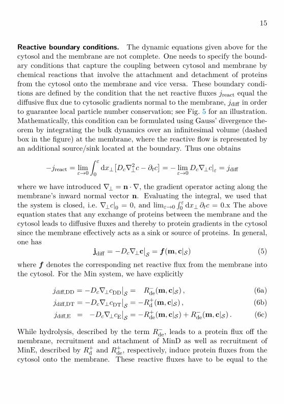
Reactive boundary conditions. The dynamic equations given above for thecytosol and the membrane are not complete. One needs to specify the bound-ary conditions that capture the coupling between cytosol and membrane bychemical reactions that involve the attachment and detachment of proteinsfrom the cytosol onto the membrane and vice versa. These boundary condi-tions are defined by the condition that the net reactive fluxes jreact equal thediffusive flux due to cytosolic gradients normal to the membrane, jdiff in orderto guarantee local particle number conservation; see Fig. 5 for an illustration.Mathematically, this condition can be formulated using Gauss’ divergence the-orem by integrating the bulk dynamics over an infinitesimal volume (dashedbox in the figure) at the membrane, where the reactive flow is represented byan additional source/sink located at the boundary. Thus one obtains

−jreact = limε→0

∫ ε

0dx⊥

[Dc∇2

⊥c− ∂tc]

= − limε→0

Dc∇⊥c|ε = jdiff

where we have introduced ∇⊥ = n · ∇, the gradient operator acting along themembrane’s inward normal vector n. Evaluating the integral, we used thatthe system is closed, i.e. ∇⊥c|0 = 0, and limε→0

∫ ε0 dx⊥ ∂tc = 0.x The above

equation states that any exchange of proteins between the membrane and thecytosol leads to diffusive fluxes and thereby to protein gradients in the cytosolsince the membrane effectively acts as a sink or source of proteins. In general,one has

jdiff = −Dc∇⊥c∣∣S = f(m, c|S) (5)

where f denotes the corresponding net reactive flux from the membrane intothe cytosol. For the Min system, we have explicitly

jdiff,DD = −Dc∇⊥cDD∣∣S = R−de(m, c|S) , (6a)

jdiff,DT = −Dc∇⊥cDT∣∣S = −R+

d (m, c|S) , (6b)jdiff,E = −Dc∇⊥cE

∣∣S = −R+

de(m, c|S) +R−de(m, c|S) . (6c)

While hydrolysis, described by the term R−de, leads to a protein flux off themembrane, recruitment and attachment of MinD as well as recruitment ofMinE, described by R+

d and R+de, respectively, induce protein fluxes from the

cytosol onto the membrane. These reactive fluxes have to be equal to the

16

diffusive fluxes of the corresponding protein species. Equation (6a) states thatdetachment of MinD-ADP following hydrolysis on the membrane, jreact,DD =R−de = kdemde > 0, is balanced by gradients of MinD-ADP in the cytosol,jdiff,DD = −Dc∇⊥cDD|S . This means that there is a negative gradient of cDDfrom the membrane into the cytosol, i.e. a surplus of inactive MinD closeto the membrane. For active MinD there is a depletion zone close to themembrane as attachment and recruitment imply a flux of proteins from thecytosol onto the membrane. Finally, the diffusive fluxes of MinE in the cytosolequals the difference in the reactive flux due to hydrolysis and the reactive fluxcorresponding to MinE recruitment by MinD. As the reactive fluxes for therespective protein states in the cytosol play a similar role as the reactionterms Rmem for the protein states on the membrane, we have introduced thenotation: jdiff. Accounting for the reactive and latent MinE states individuallythe last of the above boundary conditions generalises to

−Dc∇⊥cEr∣∣S = −R+

recruit,Er(m, c|S) +R−de(m, c|S) ,−Dc∇⊥cEl

∣∣S = −R+

recruit,El(m, c|S) .

In most of the following, we do not account for the extended bulk but studydynamics where gradients normal to the membrane can be neglected. Still, itis important to keep in mind that this is not always possible. We will later,in Sec. 5, come back to the discuss situations where these gradients, inducedby the bulk-boundary coupling, play an important role.

Mass-conservation. The coupled reaction-diffusion dynamics on the mem-brane and in the cytosol conserve the protein numbers

ND =∫V

d3x cDD + cDT +∫S

d2xmd +mde , (7a)

NE =∫V

d3x cE +∫S

d2xmde . (7b)

It will turn out later, that mass conservation will be essential in arriving at asystematic understanding of the mechanisms leading to pattern formation.

17

b bulk

x

yz

membrane

MinD membrane density

hcytosol

membrane

ain vivo in vitro

pole-to-poleoscillations

Figure 6. Simulation snapshots of the Min system (performed in COMSOL Multi-physics using the parameters given in Table 1). The rod shape of E. coli is approxi-mated by an ellipse in a reduced two-dimensional geometry, where the third spatialdimension is integrated out. The green arrow indicates the propagation direction oftraveling waves in vitro. Note the vast difference in spatial scale between the twoscenarios. For details and movies of the dynamics see [18] and [37] respectively.

Finite element simulations. Reaction–diffusion models with bulk-surface cou-pling can be simulated numerically using finite element methods. For illus-tration, Fig. 6 shows snapshots from simulation results of the Min system[Eqs. (2), (4), (6)] for a reduced two-dimensional in vivo geometry [18] and athree-dimensional in vitro box geometry [37]. The model parameter used forthe in vitro setup are listed in Tab. 1.

The main insights obtained from the numerical analysis of the effective two-dimensional in vivo model were the following [18]: Four molecular processes— membrane recruitment of MinD, formation of MinDE complexes by recruit-ment of MinE, detachment of MinDE complexes, and nucleotide exchange ofMinD in the cytosol — suffice to reproduce all oscillatory patterns as well astheir observed temperature dependence. The essential nonlinearities in thesystem come from cooperative recruitment of cytosolic MinD and MinE to themembrane by membrane-bound MinD. Two conditions turn out to be crucialfor robust pattern formation. First, MinD recruitment cannot be too weak in

18

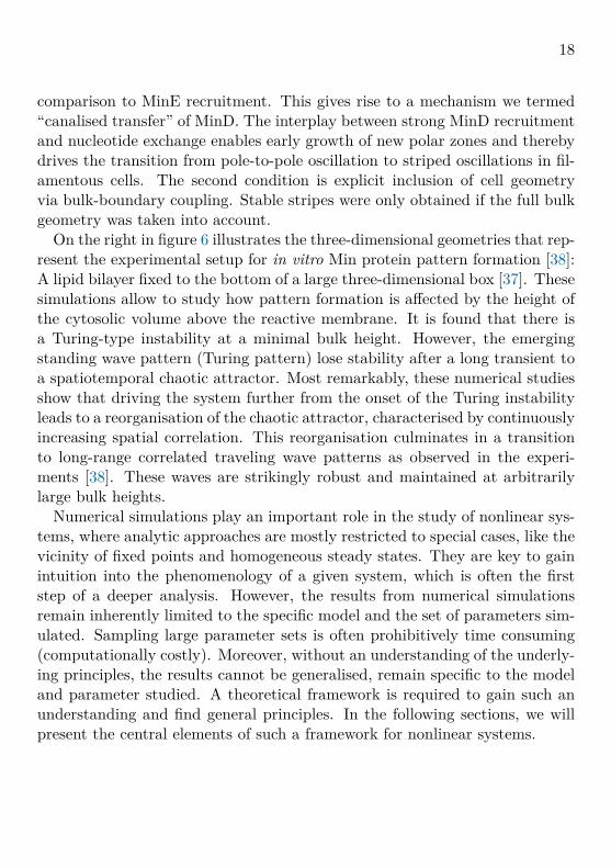
comparison to MinE recruitment. This gives rise to a mechanism we termed“canalised transfer” of MinD. The interplay between strong MinD recruitmentand nucleotide exchange enables early growth of new polar zones and therebydrives the transition from pole-to-pole oscillation to striped oscillations in fil-amentous cells. The second condition is explicit inclusion of cell geometryvia bulk-boundary coupling. Stable stripes were only obtained if the full bulkgeometry was taken into account.

On the right in figure 6 illustrates the three-dimensional geometries that rep-resent the experimental setup for in vitro Min protein pattern formation [38]:A lipid bilayer fixed to the bottom of a large three-dimensional box [37]. Thesesimulations allow to study how pattern formation is affected by the height ofthe cytosolic volume above the reactive membrane. It is found that there isa Turing-type instability at a minimal bulk height. However, the emergingstanding wave pattern (Turing pattern) lose stability after a long transient toa spatiotemporal chaotic attractor. Most remarkably, these numerical studiesshow that driving the system further from the onset of the Turing instabilityleads to a reorganisation of the chaotic attractor, characterised by continuouslyincreasing spatial correlation. This reorganisation culminates in a transitionto long-range correlated traveling wave patterns as observed in the experi-ments [38]. These waves are strikingly robust and maintained at arbitrarilylarge bulk heights.

Numerical simulations play an important role in the study of nonlinear sys-tems, where analytic approaches are mostly restricted to special cases, like thevicinity of fixed points and homogeneous steady states. They are key to gainintuition into the phenomenology of a given system, which is often the firststep of a deeper analysis. However, the results from numerical simulationsremain inherently limited to the specific model and the set of parameters sim-ulated. Sampling large parameter sets is often prohibitively time consuming(computationally costly). Moreover, without an understanding of the underly-ing principles, the results cannot be generalised, remain specific to the modeland parameter studied. A theoretical framework is required to gain such anunderstanding and find general principles. In the following sections, we willpresent the central elements of such a framework for nonlinear systems.

19

Symbol Unit Value Description

h µm 30 Bulk heightnD µm−3 638 Total MinD densitynE µm−3 410 Total MinE densityDm µm2 s−1 0.013 Membrane diffusionDc µm2 s−1 60 Cytosol diffusionλ s−1 6 Nucleotide exchangekD µm s−1 0.065 Spontaneous MinD attachmentkdD µm3 s−1 0.098 MinD self-recruitmentkdE µm3 s−1 0.126 Recruitment of MinE by MinDkde s−1 0.34 MinDE complex dissociation

Table 1. Standard parameters for the Min skeleton model in the in vitro setting.

3 Protein reaction kineticsThis chapter serves as an introduction to the most important concepts ofdynamic system theory. It builds on material discussed in standard textbooks[39, 40], but tries to put an emphasis on those concepts that are needed forthe analysis of mass-conserving systems.

3.1 Rate equations for well-mixed biochemical systemsA network of biomolecular reactions typically consists of a set of elementaryreactions including processes like degradation (A −→ ∅), production (∅ −→ A),birth/autocatalysis (A −→ 2A), dimer formation (A + B −→ AB) and con-formational changes (A −→ A∗). Here we are interested in protein reactionnetworks of the type illustrated in Fig. 2. In this section we will discusshow to analyse the dynamics of such networks in well-mixed systems, i.e. weassume that the size of the reaction compartment is much smaller than alldiffusive length scales. Then, given a set S of chemical species with concen-trations u = {ui(t)}i∈S , the dynamics is given by a system of coupled ordinary

20

differential equations (ODEs)

∂tu(t) = f(u(t);µ

), (8)

where the parameters µ ∈ RNp denote the kinetic rate constants for the variouschemical processes; Np is the number of kinetic parameters. For a given bio-chemical reaction scheme, one can readily find these equations, called chemicalrate equations, using the law of mass action.1 We have seen examples alreadywhen we discussed the reaction scheme for the Min system in Section 2.3.

There is an elaborate mathematical theory, called dynamic system theory,that allows to analyse systems of coupled nonlinear ordinary differential equa-tions. The basic idea of this theory, going back to the pioneering work ofPoincare [41], is to characterise the system’s dynamics in terms of geomet-ric structures in the phase space spanned by the set of dynamic variables{ui(t)}. In the following we will give a concise overview of dynamic systemtheory, restricting ourselves to simple systems with only one or two dynamicvariables. The interested reader will find further information in introductorytextbooks [39, 40] or more advanced monographs [12, 42].

A solution u(t) of the ordinary differential equation Eq. (8) is a curve in R|S|parametrised by time t (also called orbit in phase space). One may specify aninitial condition u(t0) = u0 at some time t0, which is often (for autonomoussystems) conveniently chosen as t0 = 0. A set of curves u(t) corresponding toa set of different initial conditions is called a flow in phase space, cf. examplesshown in Fig. 7. The goal of dynamic systems theory is to find a geometricalcharacterisation of the flow in phase space, which is sometimes also calledthe phase portrait. In other words, one would like to answer questions of thetype: How does an orbit u(t) depend on the initial condition u0? How doesthe phase portrait change qualitatively under variation of control parameterslike the kinetic rates µ? What ‘types’ of flow profiles are possible, i.e. can wegeometrically classify the phase portraits? What is the asymptotic behaviourof the orbits as t → ∞, i.e. what are the ‘attractors’ of the dynamics? Canone characterise and classify transitions between attractors?

1 The law of mass action by Guldberg-Waage assumes that the rate of a chemical reactionsis directly proportional to the product of the densities of the reacting species. In general,it is only valid if correlations can be neglected.

21

0 2

2

0u

v

0 4

4

0u

v

Figure 7. Visualisation of the phase space flow for two-variable dynamic systemsproduced by Mathematica’s StreamPlot function. (Left) The system defined by ∂tu =−u + u2v, and ∂tv = u − v has a saddle point at (u, v) = (1, 1) and a stable fixedpoint at (u, v) = (0, 0). (Right) The ‘Brusselator’ defined by ∂tu = µ+u2v− (λ+ 1)uand ∂tv = λu− u2v with µ = 1 and λ = 2.3 exhibits limit cycle oscillations (red line)and has an unstable fixed point at (u, v) = (1, λ/µ).

3.2 One-component systemsTo familiarise ourselves with some basic concepts of nonlinear dynamics westudy one-dimensional systems, i.e. ordinary differential equations with a sin-gle dynamical variable u and a single control parameter µ:

∂tu(t) = f(u(t), µ

), (9)

where f(u, µ) is some nonlinear function; an example is shown in Fig. 8.Graphically it is trivial to find the fixed points (equilibria) of Eq. (9), andcharacterise their stability: The fixed points u∗ are given by the intersectionsof f(u) with the u-axis, f(u∗) = 0, and it is simply the sign of f(u) whichdetermines whether the dynamic variable u decreases or increases; for an illus-tration see Fig. 8. Generically, at the fixed points, the function f has a finiteslope f ′(u∗) 6= 0. Only at specific values of the control parameter µ, the firstor higher order derivatives of f at fixed points may vanish. These special pa-

22

rameter values mark bifurcations where the flow changes qualitatively. This isillustrated by the dashed curve in Fig. 8. At this special point the function f istangential to the u-axis such that f ′(u∗) = 0. Upon further shifting the curvef down the two rightmost fixed points are lost. This is called a saddle-nodebifurcation and will be discussed in more detail below.

Before we continue with a discussion of the possible bifurcation scenarios,let us briefly remark that one-dimensional systems are special as the dynamicscan always be written in the form

∂tu = −∂uV (u) .

where V (u) = −∫

duf(u). This equation can be interpreted as the dynamics ofan overdamped particle (with friction coefficient ζ = 1) moving in a potentiallandscape given by V (u), c.f. Fig. 8. Locally stable and unstable fixed pointsthen correspond to local minima and maxima of the potential V (u). In general,this analogy only holds for one-dimensional systems. For higher dimensionalsystems certain conditions have to be met for the dynamics to be formulated interms of a dynamics in a potential landscape. If such a formulation is possible,

∂tu = f(u)

u

V (u)

u

Figure 8. Illustration of flow and fixed points for a one-component dynamical system.(Left) Flow diagram: The blue arrows indicate the direction of the velocity ∂tu of thedynamic variable u. Filled and open symbols correspond to stable and unstable fixedpoints (equilibria), respectively. (Right) Potential landscape: The dynamics can beinterpreted as particles rolling into the minima of a potential V (u). Changes in thecontrol parameter µ lead to abrupt and qualitative changes in the flow of the dynamicvariable u (the particle’s dynamics) at some threshold values, called bifurcation points(see dashed curves).

23

u = f(u;µ < 0)

u

u = f(u;µ = 0)

u

u = f(u;µ > 0)

u

Figure 9. Normal form of a saddle-node bifurcation, f(u, µ) = −µ + u2, forcontrol parameters µ < 0 (left), 0 (center), and µ > 0 (right). The flow changesqualitatively at the bifurcation point µc = 0.

then the dynamics is called relaxational dynamics.

Saddle-node bifurcation. Consider the ordinary differential equation

∂tu = −µ+ u2 , (10)

with f(u, µ) = −µ + u2 shown in Fig. 9 for different values of the controlparameter µ. While for µ < 0 there are no intersections of f(u) with theu-axis and hence no fixed points, there are two fixed points at u∗ = ±√µ forµ > 0. At µ = 0, these fixed points coalesce into a half-stable fixed point atu∗ = 0. We say that a bifurcation occurs at the threshold (or critical) valueµc = 0 since the vector field in phase space is qualitatively different for µ > 0and µ < 0.

The stability of the fixed points can either be directly read off from the signof f(u) in Fig. 9, or by performing a linear stability analysis. To this end weconsider small deviations δu := u − u∗ from a given fixed point u∗ and askwhether the dynamics drives the system back to this fixed point or away fromit. Upon Taylor expanding f(u) close to the fixed point one finds

∂t δu = f ′(u∗) δu+O(δu2) ,

where f ′(u∗) = ∂uf∣∣u∗

= 2u∗ = ±2√µ. Hence u∗ = −√µ is a linearlystable, and u∗ = √µ a linearly unstable fixed point as the corresponding valuesof f ′(u∗) are negative and positive, respectively. This type of bifurcationat µc = 0 is called a saddle-node bifurcation, since at the bifurcation point

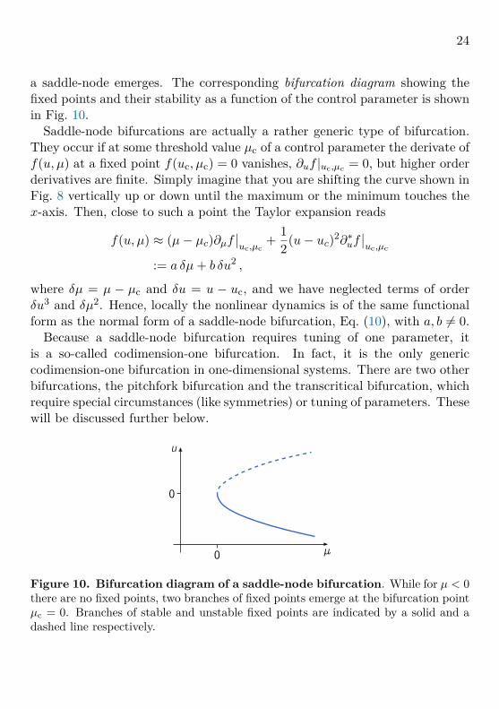
24

a saddle-node emerges. The corresponding bifurcation diagram showing thefixed points and their stability as a function of the control parameter is shownin Fig. 10.

Saddle-node bifurcations are actually a rather generic type of bifurcation.They occur if at some threshold value µc of a control parameter the derivate off(u, µ) at a fixed point f(uc, µc) = 0 vanishes, ∂uf |uc,µc = 0, but higher orderderivatives are finite. Simply imagine that you are shifting the curve shown inFig. 8 vertically up or down until the maximum or the minimum touches thex-axis. Then, close to such a point the Taylor expansion reads

f(u, µ) ≈ (µ− µc)∂µf∣∣uc,µc

+ 12(u− uc)2∂∗uf

∣∣uc,µc

:= a δµ+ b δu2 ,

where δµ = µ − µc and δu = u − uc, and we have neglected terms of orderδu3 and δµ2. Hence, locally the nonlinear dynamics is of the same functionalform as the normal form of a saddle-node bifurcation, Eq. (10), with a, b 6= 0.

Because a saddle-node bifurcation requires tuning of one parameter, itis a so-called codimension-one bifurcation. In fact, it is the only genericcodimension-one bifurcation in one-dimensional systems. There are two otherbifurcations, the pitchfork bifurcation and the transcritical bifurcation, whichrequire special circumstances (like symmetries) or tuning of parameters. Thesewill be discussed further below.

0

0

Figure 10. Bifurcation diagram of a saddle-node bifurcation. While for µ < 0there are no fixed points, two branches of fixed points emerge at the bifurcation pointµc = 0. Branches of stable and unstable fixed points are indicated by a solid and adashed line respectively.

25

(a) (b)

Figure 11. Graphical analysis of fixed points for the cusp normal form. Theintersection of the graphs for y1(u) = −h (red) and y2(u) = ru− u3 (blue) determinethe location of the fixed points, and stability can be inferred from the slope of y2(u).(a) For r < 0, there is only one stable fixed point (filled circle), independent of themagnitude of h. (b) For r ≥ 0, there are up to three fixed points depending on themagnitude of h. While for |h| > hc(r), there is only one stable fixed point, there arethree fixed points in the regime |h| < hc(r): stable fixed points on the left and rightbranch u∗±(h) indicated by the solid circles, and an intermediate unstable fixed pointu∗0(h), indicated by the open circle. At |h| = hc(r) there are saddle-node bifurcations.

The cusp bifurcation, bistability, and catastrophes. Next, we discuss anexample of a codimension-two bifurcation, the so called cusp, whose normalform is given by

∂tu = ru− u3 + h , (11)

where r and h are control parameters. As we will see, it has a close relationshipwith the saddle-node bifurcation. One may also rewrite the dynamics Eq. (11)in terms of a potential V (u) which has the form of a Landau free energy foran Ising model in an external magnetic field h: V (u) = −1

2ru2 + 1

4u4 − hu.

The fixed points of Eq. (11) can be determined graphically as the intersec-tions between the functions y1(u) = −h and y2(u) = ru − u3, as illustratedby the red and blue curves in Fig. 11, respectively. For r < 0 (‘paramagneticphase’), the function y2(u) = ru − u3 is monotonically decreasing in u, andhence there is only one stable fixed point u∗, given by u∗ ≈ −h/r for smallh. In contrast, for r > 0, there may be up to three fixed points dependingon the magnitude of the control parameter h. For large values of |h|, there is

26

only one fixed point and it is stable. Upon lowering h, there are saddle-nodebifurcations when y1(u) = −h becomes tangential to y2(u) = ru − u3. Thiscondition determines two lines of saddle-node bifurcations, h = ±hc(r), in theparameter plane, with hc(r) = 2 (r/3)3/2.

In the parameter regime |h| < hc(r), the dynamics is bistable with two stablefixed points u∗±(h) separated by an unstable fixed point u∗0(h). The bistableregime ends in a cusp at (r, h) = (0, 0), where the two lines h = ±hc(r)meet. This bifurcation scenario is visualized in Fig. 12a, showing the surfaceof fixed points u∗(r, h) over the (r, h) parameter plane. The line of saddle-nodebifurcations (blue line) is where the slope of the surface becomes vertical. Thecusp point is where the line of saddle-node bifurcations itself becomes vertical.

While for r < 0 (‘paramagnetic phase’) one may continuously change thefixed point value from positive to negative values upon lowering h, this is notpossible for r > 0 (‘ferromagnetic phase’). Here, starting with a fixed pointon the upper branch and lowering h there is a threshold value −hc(r) wherethe upper branch disappears (saddle-node bifurcation), and as a consequencethe dynamic variable changes abruptly to the lower branch (see Fig. 12b).This is sometimes also called a ‘catastrophe’ [10]. Increasing h again after thecatastrophe, the system will remain in the lower branch up to the saddle-nodebifurcation at hc(r). This behaviour is called hysteresis.

A new type of bifurcation, called pitchfork bifurcation, takes place if onepasses exactly through the cusp point, tangentially to the saddle-node linesmeeting there in the parameter plane. Here, this corresponds to keeping h = 0constant and varying r (see Fig. 12c). In this case there is inversion symmetryin u. Any h 6= 0 breaks this symmetry such that the system undergoes asaddle-node bifurcation instead of a pitchfork bifurcation (this is sometimesreferred to as ‘imperfect pitchfork bifurcation’ [39]). In general, a pitchforkbifurcation requires fine tuning or the presence of a symmetry. In the cuspnormal form Eq. (11), tuning h = 0 encompasses both, as it corresponds to asituation where a symmetry (u→ −u) is present.

27

u

r

h

SN

SN

cusp

0 0r

0

u

(a)

(c)

(b)u

h0

SN

SN0

0

Figure 12. Cusp bifurcation scenario. (a) Surface of fixed point u∗(r, h). Twolines of saddle-node bifurcations (SN, blue lines) emanate from the cusp point at(r, h) = (0, 0). In the regime enclosed by the saddle-node bifurcations (shaded in grayin the parameter plane), the system is bistable, while it is monostable everywhere else.(b) Bifurcation diagram u∗(h) for r > 0: For |h| > hc(r) the system is monostable,and becomes bistable in the domain |h| < hc(r) with two stable fixed points separatedby an unstable fixed point. Upon first increasing h through one of the SN bifurcationsand then back again, there is hysteresis as indicated by the red arrows. (c) Pitchforkbifurcation in r for the special case h = 0, where the system is symmetric underu→ −u. In general, a system undergoes a pitchfork bifurcation if one passes throughthe cusp tangentially to the SN lines meeting there.

28

Transcritical bifurcation. Consider the following reaction scheme

M + C λ−→ M + M ,

M δ−→ C .

This may be viewed as the dynamics of a one-protein system, where the proteincan be in two distinct states M and C. These states may be considered as activeand inactive states or as membrane-bound (M) and cytosolic (C) states. Inthe latter case, one may read the first reaction as a recruitment process wheremembrane-bound proteins recruit cytosolic proteins to the membrane witha rate λ, and the second reaction as detachment of these membrane-boundproteins back into the cytosol with rate δ. The corresponding rate equationsread (assuming a well-mixed compartment)

∂tm(t) = λmc− δ m ,

∂tc(t) = −λmc+ δ m ,

where m and c denote the number of proteins on the membrane and in the cy-tosol, respectively. The process defined by the reaction scheme above can alsobe interpreted as a contact process, a model for the dynamics of an infection.2Then C is a healthy person infected by a sick person M, λ is the infection rate,and δ is the recovery rate.

The dynamics conserves the total number of individuals, as the total numbern = m+ c remains invariant: ∂tn = 0. Thus the dynamics reduces to a singleequation

∂tm = λm(n−m)− δ m =: f(m) .

The fixed points (∂tm = 0) are given by

m∗1 = 0 , m∗2 = n− δ

λ,

2 Instead of a disease spreading in a population you may also consider the spreading ofopinions. Of course, spreading of diseases and opinions in a population is affected bya plethora of factors, e.g. the spatial distribution of people, how they are connectedthrough social networks, and physical constitution resp. personality.

29

m∗

nnc =

δλ

m∗

δ

λ

n

n

Figure 13. Bifurcation diagram of the contact process. (Left) As a function ofpopulation size the infection spreads only if the size exceeds a threshold size given bync = δ/λ. (Right) For a given population size n, the infection spreads if the recoveryrate is smaller than the infection rate, δ/λ < n.

corresponding to a state where there are no proteins on the membrane and astate where a finite fraction of proteins is on the membrane. We may easilycheck their stability upon calculating the first derivative f ′(m) = λ (n−2m)−δat the respective fixed points. One finds

f ′(m∗1) = λn− δ ,f ′(m∗2) = δ − λn ,

such that m∗2 is stable while m∗1 is unstable for n > δ/λ and vice versa forn < δ/λ, i.e. the fixed points interchange their stability at nc = δ/λ. This iscalled a transcritical bifurcation; see Fig. 13.

This result may be interpreted in various ways. First, let’s say that the re-cruitment (infection) rate and the detachment (recovery) rate are both fixed.Then nc = δ/λ denotes a threshold value for the protein number (popula-tion size), above which proteins start to attach to the membrane (an infectionspreads in the population). The number of membrane-bound proteins (sickpeople) is then given by m∗ = n − δ/λ. Below the threshold nc, the wholepopulation will eventually become healthy. Second, for a given protein num-ber (population size) n, it depends on the ratio of detachment (recovery) torecruitment (infection) rate whether proteins attach to the membrane (theinfection may spread in the population). While for low detachment (recovery)

30

rate µ/λ < n protein bind to the membrane (the infection spreads), the mem-brane remains devoid of proteins (the infection will be eliminated) for highdetachment (recovery) rate, δ/λ > n.

Exercise 1. Perform a bifurcation analysis of the set of equations

∂tm(t) = λm2 c− δ m∂tc(t) = −λm2 c+ δ m

where a stronger nonlinearity than above has been assumed for the re-cruitment term. What kind of bifurcation does the system exhibit?

Exercise 2. Consider a basic model of a growing microtubule with alimited amount L of tubulin dimers in the confined volume of a cell. Tostudy the dynamics of the microtubule length l in an elementary sce-nario, assume that the depolymerisation rate δ is constant while thepolymerisation rate is resource limited, γ(l) = γ0(L−l). Then the growthdynamics of the microtubule is given by

∂t l(t) = γ(l)− δ .

Discuss the dynamics as a function of the reaction rates γ0 and δ as wellas the amount of limited resources (tubulin dimers) L. What kind ofbifurcation does the system exhibit? What does this imply for the possi-bility of controlling the length of a microtubule?

General two-component systems with mass conservation. We consider ageneral two-component system with mass conservation

∂tm(t) = +f(m, c) , (12a)∂tc(t) = −f(m, c) . (12b)

31

In the biological context of cell polarisation, the nonlinear kinetics term f(m, c)is typically of the form

f(m, c) = a(m) c− d(m)m,

where the non-negative terms a(m) and d(m) denote the rates of attachmentof proteins from the cytosol to the membrane and detachment back into thecytosol, respectively. For example, one may assume a reaction kinetics withautocatalytic recruitment (Michaelis–Menten kinetics with Hill coefficient 2)and linear detachment [43]

f(m, c) =(kon + kfb

m2

K2d +m2

)c− koff m. (13)

Measuring time in units of the inverse off-rate k−1off , and densities in units of

Kd, this expression can be made non-dimensional

f(m, c) =(κ+ κfb

m2

1 +m2

)c−m, (14)

with κfb := kfb/koff and κ := kon/koff . In the following, we will for illustra-tion purposes often use the case κfb = 1, leaving κ as the only free kineticparameter.

The reaction kinetics, Eq. (12), can be analysed in (m, c)-phase space usinggeometric reasoning; see Fig. 14. As the dynamics conserve the total proteinnumber (protein mass), the flow in phase space is constrained to subspaces(1-simplices) where m+ c = n, henceforth called reactive subspaces (Fig. 14a).The flow in phase space vanishes along the reactive nullcline (NC) f = 0. Fora given protein mass n, the fixed points (m∗, c∗) are given by the intersectionsof the reactive nullcline f(m∗, c∗) = 0 with the reactive subspace m∗+ c∗ = n.Because the fixed points are determined by a balance of reactive flows, we callthem (reactive) equilibria.3 The dynamics (reactive flow) within each mass-conserving subspace is organised by the position, number, and stability of thereactive equilibria, as illustrated in Fig. 14.

3 The term equilibria in the sense of dynamical systems, as we use it here, is not to beconfused with thermal equilibria.

32

n

c

m

c(m,c)-phase space bifurcation diagram

reactive flow

reactive phase spaces

(un)stable reactive equilibria( )

SN

SN

Figure 14. Phase space and bifurcation structure of a well-mixed, mass-conserving two-component system. The total density n is a control parameterof mass-conserving reactions. The properties (number, position, and stability) of thereactive equilibria depend on the total density (mass) in a well-mixed compartment.The conservation law m+ c = n is geometrically represented by 1-simplexes in phasespace, where each value of the total density corresponds to a unique 1-simplex. Werefer to these subspaces as reactive phase spaces (local phase spaces in context ofspatially extended systems). Local reactions interconvert the conformational statesof the proteins and hence change their densities, giving rise to a flow in phase space(red arrows) which, due to mass conservation, is confined to the reactive phase spaces.The flow vanishes along the reactive nullcline f(m, c) = 0 (black line) which is a lineof reactive equilibria. Each intersection of a reactive phase space with the reactivenullcline is a reactive equilibrium (m∗(n), c∗(n)) for a given total density n (shownas disks, •/◦, for three different values n1, n2, and n3). The (m, c)-phase portraitcan be transformed into a bifurcation diagram c∗(n) by the (skew) transformationn = m + c. Because of the conservation law, the well-mixed system has only onedegree of freedom, so the only possible bifurcations are saddle-node bifurcations (SN)where the reactive nullcline is tangential to a reactive phase space. Adapted from[15].

33

Using mass conservation, the reaction dynamics can be written solely interms of m(t):

∂tm(t) = f(m(t), n−m(t)

).

This form makes explicit that in addition to the chemical rates also the totalprotein density n is a control parameter. In the vicinity of an equilibrium m∗

the linearised reactive flow reads

∂tm ≈ (fm − fc) ·(m−m∗(n)

)=: σloc(n) ·

(m−m∗(n)

),

with the eigenvalue given by σloc(n) := fm − fc and the partial derivativesdefined as fm,c := ∂m,cf |(m∗,c∗); in the above formulas we have also madeexplicit that both the position and the stability of the equilibria depend onthe protein mass n. The equilibria are stable if σloc(n) < 0 and unstable ifσloc(n) > 0. The stability condition can be given a geometric interpretationin terms of the slope snc(n) of the reactive nullcline that is given by

snc(n) = ∂mc∗(m)

∣∣n

= −fmfc

∣∣∣n. (15)

For specificity consider the case of an attachment–detachment kinetics wherefc = a(m) > 0. Then, the condition for linear stability (σloc(n) < 0) can bewritten as

snc(n) = −fm/fc > −1 . (16)

Geometrically, this means that local equilibria are stable if the tangent to thereactive nullcline cuts the simplex of the reactive phase space from below, andunstable otherwise. For the example shown in Figure 14a, the dynamics ismainly monostable with only one stable fixed point (•) except for a windowof protein masses (near n2) where the dynamics exhibits bistability with oneunstable (◦) and two stable fixed points (•).

Given this geometric criterion it is straightforward to construct the bifur-cation diagram of the (reactive) equilibrium c∗(n) as a function of the totaldensity n, cf. Fig. 14b. This reiterates a point we have made earlier, namelythat the total protein density is a control parameter of the dynamics. Varyingthe total protein density, the position and number of equilibria as well as thestability of these equilibria change. This fact will turn out to be a key element

34

for understanding the mass-conserving reaction–diffusion dynamics [15, 37],as we will discuss later in these lecture notes.

Above we have analysed the well-mixed system within the reactive sub-space for a given fixed protein mass n. For the discussion of the spatiallyextended systems it will turn out to be informative to perform this analysisin the two-dimensional phase plane (m, c), as the total protein density mightbe spatially heterogeneous. Then, to study the linear stability one definesthe displacement vector δu := (m−m∗, c− c∗)T and considers the linearisedsystem corresponding to Eq. (12),

∂t δu = J δu ,

with the Jacobian given by

J =(

fm fc−fm −fc

),

with fm,c defined as above. Using the ansatz u(t) = eσt e one finds the eigen-values

σ(1) = 0 ,σ(2) = fm − fc ,

and the corresponding (not normalized) eigenvectors,

e(1) = (fc,−fm)T ,

e(2) = (1,−1)T .

The first eigenpair defines a center space that is spanned by the eigenvector e(1)

which is tangent to the line of fixed points given by the nullcline f(m, c) = 0.This also explains why the associated eigenvalue σ(1) is zero. The secondeigenpair defines the stability of the equilibrium (fixed point) against pertur-bations that preserve the total particle density n; note that the eigenvector e(2)

spans a simplex in phase space defined by the mass conservation constraintm+ c = n. The eigenvalue agrees with the one obtained above, σ(2) = σloc.

35

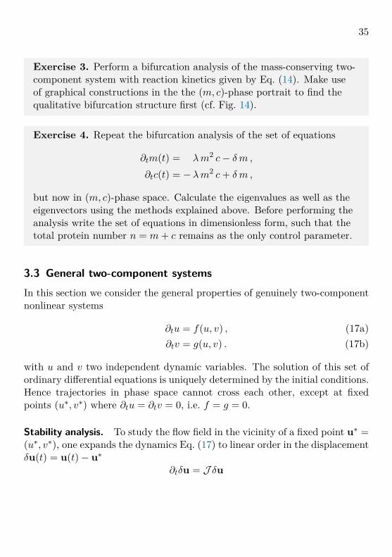
Exercise 3. Perform a bifurcation analysis of the mass-conserving two-component system with reaction kinetics given by Eq. (14). Make useof graphical constructions in the the (m, c)-phase portrait to find thequalitative bifurcation structure first (cf. Fig. 14).

Exercise 4. Repeat the bifurcation analysis of the set of equations

∂tm(t) = λm2 c− δ m ,

∂tc(t) = −λm2 c+ δ m ,

but now in (m, c)-phase space. Calculate the eigenvalues as well as theeigenvectors using the methods explained above. Before performing theanalysis write the set of equations in dimensionless form, such that thetotal protein number n = m+ c remains as the only control parameter.

3.3 General two-component systemsIn this section we consider the general properties of genuinely two-componentnonlinear systems

∂tu = f(u, v) , (17a)∂tv = g(u, v) . (17b)

with u and v two independent dynamic variables. The solution of this set ofordinary differential equations is uniquely determined by the initial conditions.Hence trajectories in phase space cannot cross each other, except at fixedpoints (u∗, v∗) where ∂tu = ∂tv = 0, i.e. f = g = 0.

Stability analysis. To study the flow field in the vicinity of a fixed point u∗ =(u∗, v∗), one expands the dynamics Eq. (17) to linear order in the displacementδu(t) = u(t)− u∗

∂tδu = J δu

36

where the Jacobian at the fixed point is given by

J = Df |0 =(∂uf ∂vf∂ug ∂vg

)∣∣∣∣∣u∗

=:(fu fvgu gv

).

The solutions of this linear system can be fully classified. We are seekingsolutions of the form δu(t) ∝ eσt e with eigenvalues σ and eigenvectors e. Thecharacteristic equation for the eigenvalues is given by det(J − σ1) = 0 andresults in a quadratic equation σ2 − τσ+ δ = 0, where τ = tr J = fu + gv andδ = detJ = fugv − fvgu. Hence the eigenvalues of J read

σ1/2 = 12(τ ±

√τ2 − 4δ

)= 1

2(τ ±√

∆),

with ∆ := τ2− 4δ the discriminant. There are three cases for the eigenvalues:

(i) σ1, σ2 ∈ R (σ1 6= σ2) if ∆ > 0(ii) σ1 = σ2 ∈ R if ∆ = 0(iii) σ1,2 complex conjugate if ∆ = 0

Moreover, the signs of Reσ1,2, which determine the stability of the fixed point,can be inferred from the signs of τ and δ. The corresponding linear flows closeto a fixed point are classified as follows (see Fig. 15). For δ < 0, the eigenvaluesσ1/2 are real and have opposite signs; hence the fixed point is a saddle point.For δ > 0, the eigenvalues σ1/2 are real with the same sign (nodes), or complexconjugates (spirals and centers). For ∆ > 0 the fixed point is a node, for∆ < 0 it is a spiral. The parabola ∆ = 0 marks the border between nodesand spirals, where so called star nodes and degenerate nodes are the respectiveborder cases. The stability of the nodes and spirals is determined by τ . Forτ < 0, both eigenvalues have negative real parts, so the fixed point is stable.Unstable spirals and nodes have τ > 0. On the half line τ = 0, δ >= 0, theeigenvalues are purely imaginary such that the fixed point is neutrally stable(called a center).

Phase-portrait analysis: nullclines and invariant manifolds.. While linearstability analysis facilitates a general classification as presented above, it only

37

saddles saddles

unstable nodesstable nodes

stable spirals unstable spirals

center

Figure 15. Classification of fixed points for two-dimensional nonlinear systems. Asa function of the Jacobian’s trace τ and determinant δ.

informs about the local properties of the flow close to fixed points. How canone gain insight into the dynamics far away from fixed points, that is, the flow’sglobal structure? It is instructive to consider the nullclines f(u, v) = 0 andg(u, v) = 0 where the flow becomes fully vertical (∂tu = 0) or horizontal (∂tv =0), respectively. Nullclines intersect at the system’s fixed points. Moreover,they partition the phase space into regions where ∂tu and ∂tv have differentsigns. This makes it possible to infer the qualitative structure of the phasespace flow.

In Fig. 16, we illustrate the basic ideas of such a phase-portrait analysis foran elementary example

∂tu = −u+ u2v , (18a)∂tv = u− v , (18b)

The nullclines are given by v = 1/u and v = u; there is also a trivial branch off = 0 where u = 0. Hence, the fixed points are given by (u∗, v∗) = (0, 0) and(u∗, v∗) = (1, 1). The nullclines partition the phase space into four quadrants

38

0 2

2

0u

v

0 2

2

0u

v

Figure 16. Illustration of a phase portrait. (Left) Nullclines of the reactionkinetics Eq. (18), shown as blue (f = 0) and orange (g = 0) lines. Their intersectionsmark two fixed points, a saddle (◦), and a stable node (•). As ∂tu and ∂tv switch signupon crossing the respective nullcline, the qualitative flow structure can be inferredfrom the nullclines as indicated by the gray arrows. (Right) Visualization of the phasespace flow with nullclines and invariant stable (green) and unstable (red) manifoldscorresponding to the saddle point.

with the gray arrows indicating the direction of flow, i.e. the signs in thevelocities ∂tu and ∂tv. These suggest that the fixed point at (u∗, v∗) = (0, 0) isstable, and the fixed point at (u∗, v∗) = (1, 1) is a saddle point. Taken togethera sketch of the flow as obtained from the nullclines (Fig. 16, left) already givesa rather decent picture of the actual flow shown in Fig. 16 on the right.

The phase portrait in Fig. 16b also shows another set of important geometriccharacteristics of the flow — stable and unstable invariant manifolds, shownas green and red lines respectively. The defining properties of these manifoldsare that they are (i) invariant under the flow and (ii) tangential to the stable/ unstable eigenspaces at fixed points. These eigenspaces are spanned bythe sets of eigenvectors associated to the sets of stable / unstable eigenvalues

39

(Reσ < 0 / Reσ > 0) respectively.4 The flow in the vicinity of the unstablemanifold is directed away from the manifold. It therefore plays the role ofa separatrix that separates the basins of attraction of different stable fixedpoints of the dynamics. Saddle points lie at the intersection of stable andunstable manifolds.

Invariant manifolds play a paramount role in the mathematical analysis ofdynamical systems — in particular in the classification and characterisationof their bifurcations — in higher dimensions. Interested readers are referredto classical, advanced textbooks on dynamical systems theory [12, 42].

Nonlinear oscillators and limit cycles. Nonlinear oscillators are genuinelydifferent from harmonic oscillators we know from classical mechanics. Tohighlight the difference let’s recall the basic results for a classical harmonicoscillator.

Harmonic oscillator. Newton’s equation of motion for a harmonic oscillatorwith mass m and spring constant k

m∂2t x = −kx

can be rewritten as a set of two first order differential equations for the positionx and the velocity v:

∂tx = v ,

∂tv = − kmx .

The steady state is x∗ = v∗ = 0, and its stability is given by the eigenvaluesof the characteristic equation∣∣∣∣∣−σ 1

− km −σ

∣∣∣∣∣ = 0 ⇒ σ± = ±i√k

m.

4 When there are neutral eigenvalues (Reσ = 0), there is also a center manifold, spannedby the eigenvectors associated to the neutral eigenvalues. The ‘reactive phase spaces’in Fig. 14 are a trivial example for center manifolds.

40

In the terminology of the previous section this corresponds to a center. Thisis related to the fact that for a harmonic oscillator the total energy is strictlyconserved,

12mv

2 + 12kx

2 = E ,

and hence the orbits in the phase plane (x, v) are cycles around the origin,each with a given energy. While the frequency ω =

√k/m is an intrinsic

feature of the harmonic oscillator, the amplitude is not since it depends onthe initial conditions x0 and v0. Moreover, in real life there is nothing like aharmonic oscillator. There is always some kind of damping such that the sumof potential and kinetic energy is actually not conserved but transformed intoheat. 5 Therefore, in order to achieve sustained oscillations in a technical or abiological system the harmonic oscillator can not be used. In the following wewill discuss how nonlinear systems give rise to robust self-sustained oscillations.

Hopf bifurcation. Before discussing biological examples, we begin by analysingnonlinear oscillations in their simplest mathematical form, also known as thenormal form [42]

∂tu = ρu− ωv + (µu− λv) (u2 + v2)∂tv = ρv + ωu+ (µv + λu) (u2 + v2) .

The origin u = v = 0 is always a fixed point, with the Jacobian given by

J = Df |0 =(ρ −ωω ρ

)with eigenvalues σ± = ρ ± iω. Here, we can have a situation where theeigenvalue’s real part passes through zero while the imaginary part ω 6= 0.

The set of dynamic equations can be considerably simplified using polarcoordinates u = c cos θ, and v = c sin θ:

∂tc = ρ c+ µ c3 , (19a)∂tθ = ω + λ c2 . (19b)

5 In the language of nonlinear dynamics, the equation of motion for the harmonic oscillatoris structurally unstable. That means, upon adding a generic small term to the equationthe dynamics change qualitatively.

41

(a) (b)

Figure 17. Hopf bifurcation. Supercritical (a) and subcritical (b) Hopf bifurca-tion. Stable and unstable fixed points and limit cycles (red) are indicated by solidand dashed lines, respectively.

The time evolution of c and θ depends only on c but not on θ. Hence wehave reduced the dynamics of c to a one-component problem as discussed inSection 3.2. Introducing a potential V (c) = −1

2ρ c2 − 1

4µ c4 corresponding to

a Ginzburg-Landau free energy function, it can also be written as Model Adynamics (for a spatially uniform system) [44]

∂tc = − ∂cV (c) . (20)

For ρ > 0 and µ < 0, it corresponds to the non-conserved gradient dynamicsof an Ising system below the critical temperature exhibiting a second orderphase transition at ρ = 0 with ρ > 0 corresponding to the low temperaturephase (see Fig. 8). Changing the sign of µ to positive values leads to unstablepotentials making it necessary to complement the potential by a c6 term witha positive coefficient. The ensuing phase transition is then a first order phasetransition. As discussed next, these features have their analogues as sub- andsupercritical pitchfork bifurcations.

Supercritical Hopf bifurcation. — We start our discussion with the caseµ < 0, where the potential V (c) has a double well form for ρ > 0 and a singleminimum for ρ < 0. Then, there is always a fixed point c∗0 = 0 whose stabilitychanges from stable at ρ < 0 to unstable at ρ > 0; compare Fig. 17a for anillustration. While for ρ < 0 this is the only fixed point of the dynamics, twonew fixed points c∗± = ±

√ρ/(−µ) emerge for ρ > 0, leading to a qualitative

change in the flow. The point ρ = 0 is called a pitchfork bifurcation. Ingeneral, both branches may have significance. For the present case, however,

42

stable LC

stable FP unstable FP

unstable LC

–0.500.5

1

0

Figure 18. Subcritical Hopf bifurcation. Bifurcation diagram for the nonlinearsystem described by Eq. (21a). The fixed point c∗0 = 0 (red line) corresponds to afixed point of the full dynamical system, Eq. (21). It is stable / unstable for ρ < 0 /ρ > 0. Including the angular variable θ, the fixed points c∗± correspond to stable andunstable limit cycles, respectively. In the parameter window ρsn = − 1

4 < ρ < 0 thedynamics is bistable: excitations of a finite magnitude are required to trigger limitcycle oscillations. Starting from ρ < 0 in the fixed point c = 0 and slowly increasingρ, a limit cycle of finite amplitude arises discontinuously upon passing through ρ = 0.

only c∗+ is relevant as c denotes a radial variable. Its linear stability can bedetermined by linearising Eq. (19a) with respect to the fixed point c∗+. Toleading order one finds for δc = c− c∗+:

∂tδc = −2ρ δc .

Hence the fixed point c∗+ is stable for ρ > 0; this is also evident from theform of the potential V (c) that exhibits two local minima at c∗± (Fig. 8).The defining feature of such a supercritical Hopf bifurcation (or, supercriticalpitchfork bifurcation if both branches are considered) is that a stable fixedpoint solution c∗+ =

√ρ/|µ| continuously branches off from the solution c∗0 = 0

at ρ = 0. This is the same phenomenology as found in continuous (secondorder) phase transitions. In the present case, combined with the solution ofthe radial equation, a closed orbit emerges for ρ ≥ 0 that traces out a circlewith radius c∗+ =

√ρ/|µ| at an angular velocity ω + λ (c∗+)2.

Subcritical Hopf bifurcation. — For the opposite case, µ > 0, the fixed pointc∗0 = 0 changes stability as before, but now the fixed points c∗± = ±

√−ρ/µ

exist only for ρ < 0. Moreover, as one can easily check, both branches c∗± are

43

unstable. This is called a subcritical Hopf (subcritical pitchfork) bifurcation,and is illustrated in Fig. 17b. The feature that the fixed point c∗+ is unstableleads to a runaway flow for c > c∗+. In order to stabilize the dynamics onemay generalise the radial equation by introducing a higher order term (forsimplicity we set µ and the prefactor of the quintic term to unity)

∂tc = ρ c+ c3 − c5 , (21a)∂tθ = ω + λ c2 . (21b)

This corresponds to a potential

V (c) = −12ρ c

2 − 14c

4 + 16c

6 ,

i.e. a Landau free-energy potential describing a first order phase transition.The fixed points for non-negative c are given by c∗0 = 0 and (c∗+)2 = 1

2±√ρ+ 1

4 .Performing a linear stability analysis (left as an exercise) yields Fig. 18. Theadditional quintic term (c5) prevents the blowup of solutions and gives rise toa new stable branch c∗+ shown as the solid blue line in Fig. 18. As a result,a limit cycle is created in a saddle node bifurcation at ρsn = −1/4. The fixedpoint at c∗0 = 0 becomes unstable at ρc = 0. Taken together, this gives rise totwo new phenomena: (i) Hysteresis: Starting from the fixed point c∗0 = 0, thisfixed point becomes unstable at ρ = 0, and the amplitude of the limit cycleoscillations discontinuously jumps to a finite value c∗+ = 1; see gray arrow inFig. 18. Then, upon reducing the control parameter ρ below 0 these limitcycle oscillations persist until one reaches ρsn = −1/4, where it then jumpsback to the stable state at c∗0 = 0 (in a saddle-node backward bifurcation). (ii)Bistability: In the parameter window ρsn < ρ < ρ < 0 the dynamics is bistable— a stable fixed point (c∗0 = 0) and a stable limit cycle (c∗+) coexist in phasespace. The unstable limit cycle at c∗− acts as a separatrix between the basinsof attraction of the fixed point and the stable limit cycle. If a system at c∗0is perturbed with a magnitude δc > c∗−, it will leave the basin of attractionof c∗0 and approach the limit cycle at c∗+. In other words, a sufficiently largestimulus is required to trigger the limit cycle oscillations in this regime.

Rho GTPase oscillators. Limit cycle oscillations are important for a range ofcellular processes, especially for controlling diverse cellular rhythms [45, 46].

44

membraneRhoGDP RhoGTP

RhoGDP

cytosolkon koff

kGEF

kGAP

Figure 19. Schematic of a Rho GTPase cycle. Inactive Rho-GDP can attachto and detach from the membrane with rates kon and koff , respectively. On themembrane, Rho gets activated by GEFs, effectively described by an autocatalyticprocess with rate kGEF = kbasal + kautom

2T. When Rho-GTP is hydrolysed with a

rate kGAP it is assumed to detach from the membrane.

Here we discuss a basic model for limit cycle oscillations of Rho GTPases,an important class of proteins that play a central role in the regulation ofcell polarity and signal transduction pathways [47]. In Section 2.1 we havealready discussed the Cdc42 system of budding yeast which is the centralprotein responsible for the self-organised establishment of a defined locationfor daughter cell growth (bud formation). Cdc42 belongs to the larger classof Rho GTPases which all share the GTPase cycle between a GDP-bound(‘inactive’) state and a GTP-bound (‘active’) state regulated by two mainclasses of proteins: Guanine nucleotide exchange factors (GEFs) promotingthe exchange of GDP for GTP, and GTPase activating proteins (GAPs) thatfacilitate hydrolysis of GTP to GDP.

Figure 19 shows a simplified reaction scheme for a Rho GTPase cycle wherethe action of the regulatory proteins is accounted for effectively [48]. Cy-tosolic, inactive Rho can attach to and detach from the membrane with rateskon and koff , respectively. On the membrane, the inactive Rho conforma-tion can get activated, either with a basal rate kbasal or mediated by GEFs.As these GEFs are typically recruited to the membrane by active Rho, thiscan be accounted for effectively by an autocatalytic process. Here we choosekGEF(mT) = kbasal + kautom

2T, where mT denotes the density of membrane-

bound Rho-GTP; other choices for the nonlinearity are possible as well. Inthe active state, Rho can undergo hydrolysis, mediated by a GAP, with ratekGAP. We assume that Rho-GTP immediately detaches from the membraneafter it is hydrolysed. The reaction rates in the model are effective rates and

45

depend on the concentrations of the regulatory proteins. The nucleotide ex-change rates will depend on the GEF concentration, and the hydrolysis rateon the GAP concentration. The above reaction scheme is a simplification ofactual biological systems for several reasons: First, the regulatory proteins areonly accounted for effectively. Second, Rho as well as the regulatory proteinsin general form interaction networks with a multitude of other proteins. Here,we disregard all these effects, as our main interest is to present a biologicallyplausible but still pedagogical example for a limit cycle oscillator.

Mathematically, the reaction network (in a well-mixed system) can be writ-ten as

∂tmT = −kGAPmT + kGEF(mT)mD , (22a)∂tmD = kon cD − koff mD − kGEF(mT)mD , (22b)∂tcD = −kon cD + koff mD + kGAPmT , (22c)

where cD denotes the cytosolic density of inactive Rho, an mD and mT themembrane density of inactive and active Rho, respectively. Mass conservationrequires that the total protein number n remains fixed:

n = cD +mD +mT . (23)

In the following we analyse a simplified version with koff = 0. We choosethe time scale such that kon = 1, and rescale n → n/

√kauto. Then, using

mass-conservation, the dimensionless form of the reaction kinetics reads

∂tmT = −µmT +(λ+m2

T)mD ,

∂tmD = n−mD −mT −(λ+m2

T)mD ,

where µ = kGAP/kon and λ = kbasal/kon. For simplicity, we specify λ = 1.Then the nullclines are given by

mD = µmT

1 +m2T

and mD = n−mT2 +m2

T, (24)

respectively (see blue and orange lines in Fig. 20b). The intersection of thenullclines defines the fixed point (reactive equilibrium). Its position and sta-bility can be changed by varying the overall protein number n (protein mass)

46

0 40

120

010 20 30

30

60

90

0 6

12

0

H

limit cycles

(a) (b)

Figure 20. Limit cycle oscillations for Rho GTPases. (a) Bifurcation dia-gram as a function of the hydrolysis rate µ and the total protein density n. In theregime shaded in blue, enclosed by a Hopf bifurcation (H), one observes limit cycleoscillations; the gray, dashed lines indicate upper and lower bounds to the stabilityboundaries as discussed in the main text. (b) Phase space portrait for n = 35 andµ = 15 (red dot in (a)). The blue and orange lines indicate the nullclines ∂tmT = 0and ∂tmD = 0, respectively. The thick, red line shows the limit cycle.

and the hydrolysis rate µ. As discussed above, the stability of the fixed pointis determined by the sign of the trace of the Jacobian:

τ = −µ+ 2m∗Tm∗D − 2− (m∗T)2 .

Solving the fixed point equations ∂tmT = ∂tmD = 0 together with the Hopfbifurcation criterion τ = 0 one obtains the locus of the Hopf bifurcation inparametric form

µHopf = 2 + 3m2T +m4

Tm2

T − 1 , nHopf = mT (3 + 5m2T +m4

T)m2

T − 1 .

The Hopf bifurcation encloses a parameter regime with τ > 0 where the reac-tion kinetics exhibits limit cycle oscillations (Fig. 20); note that within this do-main, the determinant of the Jacobian δ = (3+4m2

T+4m4T+m6

T)/(m2T−1) > 0

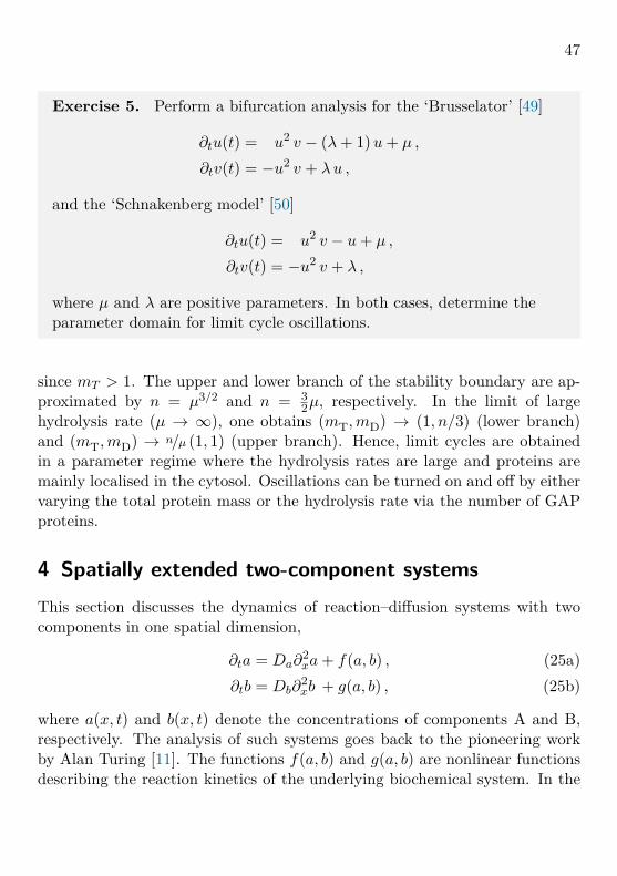
47

Exercise 5. Perform a bifurcation analysis for the ‘Brusselator’ [49]

∂tu(t) = u2 v − (λ+ 1)u+ µ ,

∂tv(t) = −u2 v + λu ,

and the ‘Schnakenberg model’ [50]

∂tu(t) = u2 v − u+ µ ,

∂tv(t) = −u2 v + λ ,

where µ and λ are positive parameters. In both cases, determine theparameter domain for limit cycle oscillations.

since mT > 1. The upper and lower branch of the stability boundary are ap-proximated by n = µ3/2 and n = 3

2µ, respectively. In the limit of largehydrolysis rate (µ → ∞), one obtains (mT,mD) → (1, n/3) (lower branch)and (mT,mD) → n/µ (1, 1) (upper branch). Hence, limit cycles are obtainedin a parameter regime where the hydrolysis rates are large and proteins aremainly localised in the cytosol. Oscillations can be turned on and off by eithervarying the total protein mass or the hydrolysis rate via the number of GAPproteins.

4 Spatially extended two-component systemsThis section discusses the dynamics of reaction–diffusion systems with twocomponents in one spatial dimension,

∂ta = Da∂2xa+ f(a, b) , (25a)

∂tb = Db∂2xb + g(a, b) , (25b)

where a(x, t) and b(x, t) denote the concentrations of components A and B,respectively. The analysis of such systems goes back to the pioneering workby Alan Turing [11]. The functions f(a, b) and g(a, b) are nonlinear functionsdescribing the reaction kinetics of the underlying biochemical system. In the

48

original paper by Turing [11] and subsequent analysis [51, 52], the functionsf and g were assumed to be independent. In these lecture notes, we areinterested in mass-conserving systems, where the spatial average of the totalprotein density n(x, t) := a(x, t) + b(x, t) is a conserved quantity:

n = 1L

∫ L

0dxn(x, t) = const.

Then, the nonlinear functions can no longer be independent but must berelated: g(a, b) = −f(a, b). Such two-component mass-conserving reaction–diffusion (MCRD) systems have been considered in the literature as ‘null-models’ of protein pattern forming systems [43, 53–62]. They have also beenstudied in the context of slime mold aggregation [63], cancer cell migration(glioma invasion) [64], precipitation patterns [65], and simple contact pro-cesses [66, 67]. Furthermore, non-isothermal solidification models [68] can alsobe rewritten in the form of MCRD equations; see e.g. Refs. [69, 70]. As willbe discussed in the following, these MCRD systems are qualitatively differentfrom models where the functions f and g are genuinely independent. Morebroadly, we will argue that reaction–diffusion systems with a mass-conserving‘core’

∂ta(x, t) = Da∂2xa+ f(a, b) + ε s1(a, b) , (26a)

∂tb(x, t) = Db∂2xb − f(a, b) + ε s2(a, b) , (26b)

are a general class of models, whose dynamics is generically driven by theinterplay between the spatiotemporal redistribution of total protein densityn(x, t) and moving local equilibria. Here, the parameter ε describes the de-gree to which mass-conservation is broken by processes like production anddegradation of proteins encoded in the source terms s1,2. For example, thereaction kinetics of the Brusselator may be written as

∂ta = −λ a+ a2 b+ ε (µ− a) , (27a)∂tb = λ a− a2 b , (27b)

where the additional terms in the dynamics of species A can be interpreted assupply of particles A from an abundant resource (εµ) and degradation (−εa).

49

As a preparation, we will recap Turing’s classical linear stability analysis forgeneral two-component reaction diffusion systems (25). This analysis showsthat diffusion can induce an instability in a system with locally stable reactionkinetics. We then turn to mass-conserving two-component systems, startingwith a brief description of their generic phenomenology, as obtained by numer-ical simulations. In particular, we illustrate how the dynamics of the spatiallyextended system can be visualized in the (m, c)-phase portrait introduced inFig. 14 and point out several key observations that motivate the subsequentanalysis in terms of phase-space geometry. As a first step to gain a deeperunderstanding of the dynamics of MCRD systems, we then repeat the linearstability in this specific case, highlighting the effect of mass-conservation onthe linear stability properties (dispersion relation and associated eigenvectors).

Both the phenomenology observed in numerical simulations and the lin-ear stability analysis suggest that lateral redistribution of the total densityn(x, t) plays a crucial role in the dynamics. Based on this insight, we dis-cuss a thought experiment that elucidates the key concept that arises frommass conservation and underlies our framework: local (reactive) equilibria.Revisiting the linear stability analysis once again, we use the local equilib-ria to explain the physical mechanism that underlies the Turing instabilityin MCRD systems. Finally, we show how an analysis based on phase-spacegeometry in (m, c)-phase space allows us to go beyond linear stability analy-sis and characterise the dynamics and final steady state (stationary pattern)in the highly nonlinear regime. The key geometric object will be a linearsubspace, called flux-balance subspace, that represents the steady-state bal-ance of diffusive fluxes in (m, c)-phase space. Intersection points between thereactive nullcline and the flux-balance subspace will act as landmark pointsfor the construction of stationary patterns. Moreover, we will show that thebalance of reactive turnovers that arises as a stationarity condition is (approx-imately) represented by a balance of areas in the (m, c)-phase portrait, akinto a Maxwell construction.

4.1 Classical Turing systemWhile an analysis of the classical Turing case can be found in many textbooks,we will still give a concise discussion here, mainly to contrast it with the mass-

50

à

`b

inhibition inhibition

activation

Figure 21. Density profiles of species A and B after some initial local perturbationin the absence of reaction kinetics. Since the diffusion constants are different, theseperturbations spread out to different length scales `b > à, leading to ‘de-mixing’ ofthe species. In an ‘activator-inhibitor’ scenario, the density profile of the activator getsself-enhanced on short scales and inhibited on large scales, indicated by the arrows.

conserving systems. Let us start with a heuristic argument. Assume that thespatially homogeneous state with uniform densities a∗ and b∗ is stable withrespect to small spatially uniform perturbations, i.e. (a∗, b∗) is a stable fixedpoint of the reaction kinetics. Henceforth, we will refer to this as local stabilityas it is a property of the local reaction kinetics. For the sake of the argument,we also assume that the reaction kinetics is characterised by a single typicaltime scale τ . Then, during that reaction time, components A and B will diffuseover diffusion length scales

à/b :=√Da/b τ .

If these length scales are approximately the same, à ≈ `b, components A andB diffuse at the same ‘speed’ such that one expects that the system remainswell-mixed and it will return back to a spatially homogeneous steady state aftersmall spatially heterogeneous perturbations. If one species, however, spreadsmuch faster (say Db � Da) then, after some reaction time τ , a local spatialperturbation will lead to largely different spatial distributions for componentsA and B with widths `b � à. In other words, diffusion leads to a ‘de-mixing’of the species as illustrated in Fig. 21.

What emerges out of this ‘de-mixing’ depends on the reaction kinetics. Con-sider the following ‘activator–inhibitor’ scenario [51]: (i) The ‘activator’ A isauto-catalytic, and also enhances the inhibitor B. (ii) The inhibitor B slows

51

down the activation process of A, i.e. there is a negative feedback. (iii) Finally,A and B also decay at some rate. The consequences of this reaction scheme onthe concentration profile of the activator are the following: In the core regionof the spatial perturbation, ` . `a, there is a surplus of activator A since theinhibitor B has spread out faster than the activator. As a consequence, theactivator concentration grows (and is finally levelled off by nonlinear terms inthe reaction kinetics). On the other hand, in the outer region ` ∼ `b there isa surplus of inhibitor leading to a depletion of the activator. Taken togetherthis leads to a density profile for the activator illustrated in Fig. 21. Sincethe region of enhanced activator concentration is surrounded by a cloud ofinhibitors, the ensuing spatial profile is argued to be rather robust to externalperturbations. For such type of reaction kinetics, the Turing mechanism issometimes also summarised as ‘short-range activation with long-range inhibi-tion leads to pattern formation’ [51, 52].

This heuristic line of argument, however, does not specify the exact con-ditions on the diffusion constants and the reaction rates that lead to patternformation. These arguments merely state that one needs some kind of ‘demix-ing’ driven by unequal diffusion constants onto which a nonlinear feedbackmechanisms can act to produce a stable pattern.

To quantify the above ideas mathematically one has to use a formal linearstability analysis, asking whether the spatially uniform steady state (a∗, b∗) isstable or unstable with respect to spatially heterogeneous perturbations, termedlateral (in)stability. To this end, we expand the reaction–diffusion equations,Eq. (25), to linear order in the deviation from the steady state, δu := (a −a∗, b− b∗)T:

∂tδu = J δu +D ∂2xδu , (28)

whereJ =

(∂af ∂bf∂ag ∂bg

)∣∣∣∣∣(a0,b0)

=:(fa fbga gb

)(29)

denotes the Jacobian of the reaction kinetics at the uniform steady state(a∗, b∗), and D = diag (Da, Db) is the diffusion matrix. Stability of (a∗, b∗)to uniform perturbations (local stability) requires that both eigenvalues σ1

52

and σ2 of the Jacobian J are negative, i.e. (compare Section 3.3)

τ0 = tr J = σ1 + σ2 = fa + gb < 0 ,δ0 = det J = σ1 · σ2 = fagb − gafb > 0 .

To study the stability against spatially inhomogeneous perturbations (lat-eral stability), the linear reaction–diffusion equations, Eq. (28), are solved byexpanding δu(x, t) in terms of the eigenmodes φq(x) of the Laplacian, fulfillingthe eigenmode equation ∂2

xφq(x) = −q2φq(x),6

δu(x, t) =∑i

∑q

A(i)q e(i)

q φq(x) exp(σ(i)q t), (30)

resulting in the eigenvalue problem

σqeq = (J −D q2)eq =: Jqeq . (31)

The eigenvalues σ(i)q are obtained from the characteristic equation

det(Jq − σqI

)= 0 . (32)

For each Fourier mode q one finds two eigenvalues

σ(±)q = 1

2(τq ±

√τ2q − 4δq

), (33)

where τq = trJq and δq = det Jq are the trace and determinant of the ma-trix Jq = J − Dq2, respectively. The eigenvalues σ(i)

q as a function of thewavenumber q constitute the so called dispersion relation. Often one is pri-marily interested in the eigenvalue with largest real part for each q since thisdetermines the stability of the cos(qx) mode.

To find the parameter regime where the homogeneous steady state is unsta-ble against spatial perturbations, we seek a condition that guarantees that oneeigenvalue σ±q is non-negative. Since we demand that the fixed point (a∗, b∗)

6 Note that the eigenmodes of the Laplacian depend on the domain geometry and theboundary conditions. This will play a critical role in Sec. 5.2 where linear stabilityanalysis is performed for bulk-surface coupled systems.

53

(a) (b)

Figure 22. (a) Determinant δq = det(J − Dq2) as a function of q2. (b) Dispersion

relation σ+q . There is a critical value for the ratio of the diffusion constants, Dcrit,

where the mode corresponding to the wavenumber qc becomes marginally stable. ForD>Dcrit, there is a band of wavenumbers [q2

1 , q22 ] where δq < 0, and, therefore, one

eigenvalue becomes positive and thereby the dynamics becomes unstable. (The plotswere generated for the Jacobian J = ((1,−1), (3, 2))T, Da = 1, and Db = 5, 7.45, 10for the gray, blue, and red line respectively.)

of the spatially uniform system is stable against uniform perturbations, wehave trJ < 0, and thus

τq := trJq = trJ − q2 trD < 0 .Hence the eigenvalue with the larger real part, σ+

q , becomes positive only if

δq = detJq =(fa −Daq

2)(gb −Dbq2)− gafb < 0 .

As shown in Fig. 22a, the δq is a parabola in q2 that opens upwards. At q= 0it takes the value δ0> 0 which is always positive since the spatially uniformstate is stable.

In order to determine when δq changes sign, we ask when the minimumvalue of this parabola first becomes negative. Setting the derivative of δq withrespect to q2 to zero, we learn that the minimum occurs at the wave number

q2∗ = faDb + gbDa

2DaDb.

The corresponding value of δq at this minimum is

δq∗ = δ0 −(faDb + gbDa)2

4DaDb.

54

This expression is negative if the inequality

faDb + gbDa >√

4DaDbδ0 (34)

is satisfied (Segel–Jackson condition [52]). This condition is necessary andsufficient for the emergence of a Turing instability. Upon defining D :=Db/Da

we may rewrite the Turing condition, Eq. (34), as faD+gb > 2√D δ0, i.e. only

the relative strength D of the diffusion constants matters. There is a criticalvalue for D (at given kinetic parameters) where the Turing instability occurs

faDcrit + gb = 2√Dcrit δ0 .

At this threshold value Dcrit, the critical wave number is

q2c = faDcrit + gb

2Dcrit=√

δ0Dcrit

.

Above this threshold value, D>Dcrit, the dispersion relation σq exhibits aband [q1, q2] of unstable modes (see Fig. 22b). While the above conditionsmathematically specify the parameter space where pattern formation is pos-sible, they do not provide conceptual insights into the underlying mechanismresponsible for the Turing instability.

Exercise 6. Perform a linear stability analysis for the Schnakenbergmodel [50]

∂ta(x, t) = Da∂2xa+ µ+ a2b− a ,

∂tb(x, t) = Db∂2xb + λ− a2b ,

where µ and λ are positive constants. Discuss the regimes of local andlateral stability. You may also want to write a computer program thatsimulates the dynamics of the model beyond the regime of linear insta-bility. What does one find?

55

4.2 Mass-conserving two-component reaction–diffusion systemsNow we turn to the analysis of two-component mass-conserving reaction–diffusion (MCRD) systems. As in Section 3.2, we consider two chemicalspecies, M and C, and refer to them as membrane-bound proteins and cytosolicproteins. Compared to an actual cellular system or reconstituted experimen-tal model system, we again use a simplified one-dimensional geometry whereproteins are confined to a domain [0, L]. The fact that membrane-bound andcytosolic proteins experience different fluid environments is accounted for bytwo different diffusion constants Dm and Dc respectively. With m(x, t) andc(x, t) denoting the local densities of components M and C, respectively, thereaction–diffusion equations read

∂tm(x, t) = Dm∂2xm+ f(m, c) , (35a)

∂tc(x, t) = Dc∂2xc − f(m, c) , (35b)

where the nonlinear function f(m, c) accounts for all chemical reactions. With-out loss of generality we assume that the relative diffusion constant D :=Dm/Dc ≥ 1. In the following we will restrict ourselves to no-flux boundaryconditions7

∂xm|0 = ∂xm|L = 0 ,∂xc|0 = ∂xc|L = 0 .

Recall from our analysis of well-mixed two-component systems with mass con-servation in Section 3.2 that the equilibria are given by the intersection of thenullcline (f = 0) with the reactive phase space (n = m+ c) for a given proteinmass n.

Phenomenology of the spatiotemporal dynamics. Before we embark on amathematical analysis, let us look at the results of a numerical simulation ofEq. (35) for a toy model with

f(m, c) =(k + m2

1 +m2

)c−m. (36)

7 Periodic boundaries can be treated analogously.

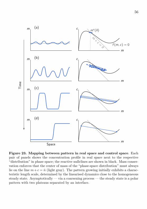
56

Spacem

cm

Tim

e

m

m

m

m

c

m

c

m

c(a)

(b)

(c)

(d)

Figure 23. Mapping between pattern in real space and control space. Eachpair of panels shows the concentration profile in real space next to the respective“distribution” in phase space; the reactive nullclines are shown in black. Mass conser-vation enforces that the center of mass of the “phase-space distribution” must alwayslie on the line m+ c = n (light gray). The pattern growing initially exhibits a charac-teristic length scale, determined by the linearised dynamics close to the homogeneoussteady state. Asymptotically — via a coarsening process — the steady state is a polarpattern with two plateaus separated by an interface.

57

Our intention is to show the phenomenology of pattern formation in real spaceand how these patterns are represented in phase space. To this end, similaras above the one-dimensional domain is dissected into a set of compartments,and the time evolution of the membrane and cytosolic density in each of thesecompartments is monitored in (m, c) phase space leading to a cloud of phasespace points. Figure 23 shows a series of snapshots that sets side by side thespatial membrane density and the corresponding distribution of phase spacepoints.

The initial concentration for the simulation displayed in Fig. 23a is a small(random) perturbation with respect to a spatially homogeneous stationarystate (m∗, c∗), indicated by the dashed line in the real space plot on the right.This steady state corresponds to the fixed point determined by the intersec-tion of the nullcline with the reactive phase space m+ c = n (gray line) in thephase portrait on the right. Initially, the dynamics exhibits a Turing insta-bility which (exponentially) amplifies the small perturbations (Fig. 23b). Theensuing initial pattern is a periodic pattern with a characteristic wavelengththat will later turn out to be the fastest growing mode as obtained from alinear stability analysis. The growing pattern entails redistribution of proteinmass, i.e. a spatially heterogeneous total density n(x, t) := m(x, t)+c(x, t). Asa consequence, the corresponding cloud of points in the phase portrait startsdeviating from the subspace m+ c = n (gray line).

After this initial phase, one observes that the points in phase space becomeconstrained to an affine subspace (i.e. a straight line) in phase space (Fig. 23c),which will later turn out to be the so-called flux-balance subspace. Withinthat subspace, the pattern’s phase-space distribution extends from one branchof the nullcline to the other. On even longer timescales the pattern profileundergoes slow coarsening dynamics until it reaches a polarised steady statewith a high and a low density separated by an interface, as shown in Fig. 23d.During the coarsening process, the distribution in phase space remains veryclose to the flux-balance subspace.

These phenomenological observations raise a set of fundamental questions:What is the mechanism underlying the pattern-forming instability from a spa-tially homogeneous state? What is driving the coarsening process from theinitial periodic pattern to the final polar pattern? Is there a way to generalise

58

the geometric phase space ideas for well-mixed systems to spatially extendedsystems? Is there a relation between the real space patterns and the attractorsobserved in phase space? What are the physical principles that determine theattractors in phase space? In the following we will address these questions.

Exercise 7. Perform numerical simulations with the reaction kinetics

f = m2c−m

from Exercise 1 and visualize the dynamics in real space and in phasespace as shown in Fig. 23. What are the qualitative differences betweenthe cases Dm � Dc and Dm . Dc? How do your findings compare to asystem with reaction kinetics given by Eq. (36)?

4.3 Linear stability analysis of mass-conserving systemsAs we have learned in the previous section, linear stability analysis of areaction–diffusion system is performed by linearising the equations with re-spect to the homogeneous steady state (m∗, c∗) and expanding a spatial per-turbation in the eigenbasis of the diffusion operator (Laplacian) in the geom-etry of the system. For a one-dimensional system with reflective boundaryconditions at x = 0 and x = L, the eigenfunctions of the Laplacian are thediscrete Fourier modes cos(qkx) where qk = kπ/L are a discrete set of wavenumbers with k ∈ N. For simplicity of notation, we suppress the subindex kin the following. The amplitudes of the Fourier modes, δmq(t), then obey thelinearised dynamics

∂t

(δmq(t)δcq(t)

)= Jq

(δmq(t)δcq(t)

)with the Jacobian

Jq =(−Dmq

2 + fm fc−fm −Dcq

2 − fc

),

where fm,c = ∂m,cf |(m∗,c∗). The eigenvalues of the Jacobian yield the growthrates σ(i)

q of the respective eigenmodes such that the time evolution of a per-

59

0

Figure 24. Turing instability in a MCRD system. Generic dispersion relationof the two-component MCRD system in a laterally unstable regime, showing the twobranches σ(1,2)

q . In the limit q → 0, the spectra σ(1,2)q reduce to the eigenvalues

σloc = fm − fc and 0 of the local stability problem, as indicated in the graph. Forfast cytosolic diffusion Dc →∞ the second branch approaches σ(2)

q → fm−Dmq2 for

q > 0 (dashed gray line), and the upper bound qmax of the band of unstable modes isgiven by

√fm/Dm. Parameters: fm = 0.7, fc = 1, Dm = 1, Dc = 10. Adapted from

[15].

turbation in the spatial eigenfunction cos(qx) is given by (cf. Eq. (30))(δmq(t)δcq(t)

)=∑i=1,2

A(i)q e(i)

q exp(σ(i)q t) cos(qx),

with the eigenvectors e(i)q associated to the eigenvalues σ(i)

q . For a given initialcondition (perturbation), the coefficients A(i)

q are determined by projecting theinitial condition onto the eigenbasis e(i)

q cos(qx). Analogous to the analysis inSec. 4.1, the eigenvalues of the Jacobian Jq can be expressed in terms of itstrace τq and determinant δq:

σ(1,2)q = 1

2(τq ±

√τ2q − 4δq

),

60

where

τq = fm − fc − (Dm +Dc)q2 = σloc − (Dm +Dc)q2 ,

δq = q2DmDc

(q2 + fc

Dc− fmDm

)= q2DmDc

(q2 − q2

max

),

and we have defined q2max = (fm/Dm)− (fc)(Dc).

We are looking for a Turing instability, i.e. for a parameter regime where oneof the eigenvalues σ(1,2)

q becomes positive at a finite value of the wave numberq, given that the homogeneous steady state is locally stable (σloc < 0). Sinceτq = σ

(1)q + σ

(2)q < 0 for all q, this is possible only if δq = σ

(1)q · σ(2)

q < 0.Hence, the discriminant ∆q = τ2

q − 4δq > 0 such that all eigenvalues must bereal. This implies that an oscillatory instability for q > 0 is excluded for alocally stable homogeneous steady state. Moreover, the instability conditionδq < 0 immediately yields the band of unstable modes [0, qmax]. Figure 24shows the two branches of eigenvalues σ(1,2)

q for such a laterally unstable case.In the limit q → 0, the first branch connects to the eigenvalue of a well-mixedsystem σ

(1)0 = σloc < 0 (cf. Sec. 3.2). The corresponding eigenvector lies in

the reactive phase space for q = 0, and hence respects mass conservation. Thesecond branch σ

(2)q remains positive as it approaches zero in the limit q→ 0.8

What is the meaning of the neutral eigenvalue σ(2)0 = 0 at q = 0? The

associated eigenvector e(2)0 points along the reactive nullcline, and thus rep-

resents homogeneous perturbations that change the average total density inthe system. The perturbed system cannot relax to the former steady state, asthis would break the conservation law. Instead, the steady state shifts alongthe reactive nullcline to a new steady state with mass n + δn. This behaviorcorresponds to the neutral eigenvalue. Importantly however, this eigenvalueis not relevant for the dynamics of a closed system since perturbations inthis case must conserve the average total mass. The homogeneous stability

8 This case is called ‘type II’ instability in the Cross–Hohenberg classification scheme [71].While type II instability is generic for two-component MCRD systems, this is not truefor systems with more components and/or multiple conserved species, where the bandof unstable modes can be bound away from zero (‘type I’ in Cross–Hohenberg scheme);see e.g. [37].

61

of closed systems is solely determined by the eigenvalue σ(1)0 whose associ-

ated eigenvector points along the reactive phase space where total density isconserved.

Spatially inhomogeneous perturbations (q 6= 0), on the other hand, redis-tribute mass laterally, such that the masses change locally. As we shall see inthe next section, introducing the notion of local reactive equilibria based onthese local masses enables us to understand the physical mechanism underly-ing the Turing instability in mass-conserving systems.

Exercise 8. Perform a linear stability analysis for the following MCRDsystem

∂tm(x, t) = Dm∂2xm+ λmac− µm ,

∂tc(x, t) = Dc∂2xc − λmac+ µm ,

for exponents a = 1 and a = 2; the parameters µ and λ are positive.Discuss the regimes of local and lateral stability. You may also want towrite a computer program that simulates the dynamics of the modelbeyond the regime of linear instability. What does one find? What hap-pens if one weakly breaks mass conservation in the linear term of thereaction kinetics or by adding an external source?

4.4 Mass-redistribution instabilityFrom the above analysis we have learned how to formally calculate the con-ditions for patterns to form spontaneously using linear stability analysis. Butwhat is the physics underlying the lateral instability driving pattern forma-tion?

Local reactive equilibria. From the mathematical linear stability analysis inthe previous section, we learned that the branch of unstable modes emergingfrom q = 0 is associated with spatial redistribution of mass, as revealed bythe direction of the corresponding eigenvector. To gain some intuition into theconsequences of lateral mass redistribution, imagine the system to be dissected

62

(a) without mass conservation

m

x

n

separate compartments

n

c

m

(m∗x, c

∗x) single global

equilibrium

(b) with mass conservation

m

x

n

separate compartments

n

c

m

(m∗x, c

∗x)

localequilibria

Figure 25. Illustration of the concept of local equilibria. Spatially extendedreaction–diffusion system dissected into small compartments (boxes) with gray scaleindicating the local protein mass n(x, t) = m(x, t) + c(x, t). Now suppose the com-partments are isolated from one another by ‘shutting off’ diffusion (indicated by solidlines between compartments). (a) In a (monostable) system without mass conser-vation, the concentrations in each compartment return to the same reactive equilib-rium, corresponding to the homogeneous steady state of the system. (b) In contrast,in a mass-conserving system the equilibrium concentrations depend on the masses(total densities) in the compartments which will in general not be distributed ho-mogeneously. This notion of local equilibria is a key concept in understanding thedynamics of mass-conserving reaction–diffusion systems (local equilibria theory).

63

into a set of small, well-mixed compartments that are coupled by diffusion;see Fig. 25 for an illustration. To highlight the role of mass conservation, wecontrast between systems that conserve mass, described by Eq. (35), and thosethat do not conserve mass, e.g. the Schnakenberg model or the Brusselator.At a given instant in time, individual protein densities as well as the totalprotein density will be spatially heterogeneous. In Fig. 25 this is illustratedby a snapshot of the density profiles for m(x, t0) and the grey scales of thecompartments for the total density n(x, t0) = m(x, t0) + c(x, t0).9

What happens if mass transport through diffusive coupling between thesecompartments is switched off? For a system without mass conservation, eachcompartment relaxes back to one and the same equilibrium (m∗, c∗) givenby the fixed point of the reaction kinetics (assuming, for simplicity, locallymonostable dynamics) with a spatially uniform mass given by n∗ = m∗ + c∗.In contrast, for mass-conserving reaction–diffusion systems, each compartmentwill remain in the local phase space determined by the local mass n(x, t0) atthe time diffusive coupling was turned off. As the masses in the differentreaction compartments are different, the dynamics will approach the reactiveequilibria (m∗x, c∗x) corresponding to the local masses n(x, t0) in each of thesecompartments; see Fig. 25. We term these equilibria local (reactive) equilibria.They are obtained from the conditions of local stationarity f(m∗x, c∗x) = 0,and local mass conservation m∗x + c∗x = n(x, t0). As in the analysis of well-mixed systems (Secs. 3.2 and 3.3), local reactive equilibria and their linearstability act as proxies for the local reactive flow within each compartment.Diffusive coupling redistributes mass laterally between the compartments, thusshifting their position in phase space and potentially changing their stability.Understanding reaction–diffusion dynamics in terms of this interplay betweenlateral mass-redistribution and moving local equilibria is the defining ideabehind local equilibria theory.

Mass-redistribution instability. Equipped with the concept of local reactiveequilibria, let us now return to the question of the physics underlying lateralinstability in MCRD systems. Consider the dynamics of the total (mass)

9 Note that we here use m and c as dynamic variables for systems with as well as withoutmass conservation.

64

density gradients: ∂xm, ∂xc mass redistribution: ∂tn

local equilibria: c∗(n(x, t)

), m∗(n(x, t)

)

Figure 26. Schematic of the interplay between mass redistribution andmoving local equilibria. Gradients in the protein densities on the membrane andin the cytosol drive the redistribution of mass which leads to a change in the localreactive equilibria. Shifted local equilibria change the local reactive flows that drivethe changes of the density gradients.

density n(x, t) = c(x, t) + m(x, t), simply obtained by adding the equationsof the membrane and cytosolic density in Eq. (35). As the reaction kineticsconserve the total density, the time evolution of the total density is driven onlyby diffusion due to spatial gradients in the concentrations c(x, t) and m(x, t):

∂tn(x, t) = Dc ∂2xc(x, t) +Dm ∂

2xm(x, t) . (37)

The spatial redistribution of protein mass also leads to a change in the con-centrations c∗(n(x, t)) and m∗(n(x, t)) of the local reactive equilibria. Theseshifting local equilibria represent the change of the local reactive flow, which— assuming stable equilibria — is directed towards them. The local reactivedynamics alter the spatial gradients in c(x, t) and m(x, t), which — in turn— drive the dynamics of the total protein density, closing the loop, as illus-trated in Fig. 26. This intricate coupling between redistribution of total mass,reactive flows, and diffusive flows drives pattern formation.

The equation for the total mass density, Eq. (37), is not closed. In orderto determine the time evolution of the total density, one needs to know thedynamics of both the membrane and the cytosolic densities. Let’s assume thatthe relaxation of the local concentrations towards the local reactive equilibriais fast compared to the lateral redistribution of protein mass. In this limit,one can make the local quasi-steady state approximation (LQSSA)

c(x, t)→ c∗(n(x, t)

), m(x, t)→ m∗

(n(x, t)

). (38)

65

which yields a closed equation for the mass density,

∂tn(x, t) ≈ Dc ∂2xc∗(n) +Dm ∂

2xm∗(n) . (39)

While this local-quasi-steady state approximation is in general not strictlyvalid, it actually becomes exact close to the onset of lateral instability sincewe have a long wavelength instability where the mass redistribution dynamicsbecomes slow; cf. Section 4.3. Moreover and more importantly, it captures theessence of the dynamics even if there is no strict separation of timescales [15].

Let’s start our analysis with the limiting case that membrane diffusion ismuch slower than cytosolic diffusion Dm � Dc (which is typical for proteinpatterns). Then, linearisation of Eq. (37) for n(x, t) = n+δn(x, t) and applyingthe chain rule yields

∂tδn(x, t) ≈ (∂nc∗|n)Dc ∂2xδn .

This is a diffusion equation with the effective diffusion coefficient Dc ∂nc∗|n

that depends on the slope of the nullcline c∗(n) at n, i.e. on how the equi-librium concentration c∗ depends on the mass n. If the equilibrium cytosolicconcentration increases with increasing mass, ∂nc∗|n > 0, the effective diffu-sion constant is positive and hence the dynamics of the total mass is stable. Incontrast, if ∂nc∗|n < 0, we have a negative effective diffusion constant whichimplies that one has a mass-redistribution instability. This shows that theinterplay between transport of mass and how the local masses changes thelocal equilibria is the core mechanism driving the dynamics and thereby pat-tern formation. This mass-redistribution instability is the physical mechanismunderlying the Turing instability found in Sec. 4.3 by a formal linear stabilityanalysis.

Figure 27 illustrates this mechanism in both real space (left panel) and inphase space (right panel) in a way that makes it intuitive. Consider a small-amplitude, long-wavelength density modulation n+ δn(x), shown as the solidpurple line in the left panel of Fig. 27. In phase space, we show the reac-tive phase spaces corresponding to the maximum and minimum values of thisdensity modulation; see the solid purple lines in the right panel of Fig. 27.As diffusive relaxation for long wavelengths is slow compared to the reactionkinetics (adiabatic limit), both the membrane and the cytosolic densities will

66

c

mSpace

Conc

entra

tion m

c

1 1 23

2

3

4

4

Figure 27. Illustration of mass-redistribution instability. Consider a smallamplitude modulation of the total density (purple line in the real space plot) on alarge length scale (1). As diffusion is slow on large scales, the system will locally relaxto its reactive equilibrium (2). The resulting cytosolic density profile is shown by theblue line in the real space plot. If the cytosolic equilibrium density decreases due to anincrease of total density, the ensuing diffusive fluxes in the cytosol (3) will amplify themodulation of the total density profile (4), thus driving an instability. The membranegradient is opposite to the cytosolic one, such that membrane diffusion counteractsthe instability. However, in the limit Dm � Dc this is negligible. In the (m, c)-phaseportrait, the criterion for this instability is that the slope of the reactive nullclinemust be negative.

first relax towards the local equilibrium values determined by the respectivelocal total protein density, as indicated by the red arrows in Fig. 27, giving riseto a modulation of the cytosolic protein density c∗(n+δn) ≈ c∗(n)+∂nc∗|n δn.For a negative nullcline slope ∂nc∗|n < 0 the modulation of the cytosolic den-sity will be in anti-phase with respect to the modulation of the total density.Hence, diffusive relaxation, according to Fick’s law, will lead to a decrease ofcytosolic density in the peaks of the total density and an increase of cytoso-lic densities where the total density is low. In addition, since Dm � Dc, themembrane density remains nearly unchanged during diffusive relaxation of thecytosolic density, such that the cytosolic diffusive fluxes translate directly intochanges of the total density; see blue arrows in Fig. 27. As a consequence, wehave a further increase in regions of high total density and a further decrease inregions of low total density. In other words, the density modulation is ampli-

67

fied, thus driving the mass-redistribution instability. Conversely, for positivenullcline slope, ∂nc∗|n < 0, the cytosolic density modulation will be in phasewith respect to the total density modulation, leading to diffusive fluxes thatcounteract the initial total density modulation. On an even more heuristiclevel, mass-redistribution instability can be understood as the self-organisedformation of spatially separated attachment and detachment zones [23].

Nullcline slope criterion for mass-redistribution instability. In the generalcase, including the effect of membrane diffusion, Eq. (37) can be rewritten as

∂tn(x, t) ≈ ∂x[(Dc ∂nc

∗ +Dm ∂nm∗) ∂xn]

which can be interpreted as a diffusion equation for the total density n(x, t)with an effective diffusion constant that depends on n(x, t). For specificity,consider the case of an attachment–detachment kinetics where fc > 0; for aconsideration of the general case please refer to [15]. Recall that then the con-dition for linear stability (σloc(n) < 0) can be written as snc(n) = −fm/fc >−1. Assuming locally stable equilibria, the effective diffusion constant willbecome negative if

∂nc∗

∂nm∗= snc(n) = −fm

fc< −Dm

Dc, (40)

where snc(n) = ∂mc∗(m)|n is the slope of the reactive nullcline c∗(m) (cf.

Eq. (15)). Hence, starting from a homogenous steady state (m∗(n), c∗(n)),lateral instability due to effective anti-diffusion takes place if (and only if)snc(n) < −Dm/Dc. This inequality translates into the geometric criterionthat the slope of the nullcline must be steeper than −Dm/Dc. Below, we willsee that this negative ratio of the diffusion constants is the slope of the socalled diffusive flux-balance subspace that geometrically encodes a balance ofdiffusive fluxes on the membrane and in the cytosol.

How do these results compare with the instability criterion obtained fromlinear stability analysis? There we found that the dispersion relation exhibitsa band of unstable modes for 0 < q < qmax, with

q2max = fm

Dm− fcDc

(41)

68

if and only if fm/Dm > fc/Dc, which is exactly the above slope criterion,Eq. (40). Importantly, the slope criterion for the mass-redistribution instabil-ity, Eq. (40), shows that the diffusion constants Dm and Dc are not requiredto be vastly different when the nullcline slope is sufficiently steep. In fact,when snc is close to −1, a ratio Dm/Dc slightly different from unity is suf-ficient. This means that the mass-redistribution instability is not hard toachieve. Nullclines with a section of negative slope, for instance, N-shapednullclines, generically arise as a consequence of nonlinear reaction kinetics andare encountered in a broad range of classical nonlinear systems.

Exercise 9. Graphically analyse the following MCRD model

f(m, c) =(k +m2) c−m

using the above geometric conditions for the existence of a mass–redis-tribution instability, i.e. draw the nullcline in (m, c) phase space and usethe slope criterion Eq. (40) for a Turing instability and the criterion forlocal stability Eq. (16). In addition, use the mathematical conditionsfor lateral stability to calculate the stability diagram as a function ofthe total protein mass n and the ratio of the diffusion constants D =Dm/Dc for two typical values of k in the locally monostable regime.

4.5 Stationary states, flux balance, and landmark pointsThe linear stability analysis performed in the previous two sections 4.3 and 4.4informs about parameter regimes where the spatially homogeneous steadystate is unstable to small spatial perturbations. This analysis, however, doesnot inform us about the dynamics beyond the initial transient close to a homo-geneous steady state. Nonlinear interactions become important with growingamplitudes of the linearly unstable modes. What are the conditions that de-termine spatially inhomogeneous stationary patterns m(x), c(x)? Our starting

69

point is the set of steady-state equations,

Dm∂2xm+ f(m, c) = 0 , (42a)

Dc∂2xc − f(m, c) = 0 , (42b)

which have to be solved given the no-flux boundary conditions and the con-straint of mass conservation.

Flux-balance subspace. Upon adding the stationarity conditions, Eq. (42),one obtains Dm∂

2xm(x) = −Dc∂

2xc(x). Using the no-flux boundary condi-

tions this can be integrated over the domain [0, x] to give a local flux-balancecondition

Dm∂xm(x) = −Dc∂xc(x) ,which is stating that locally the diffusive fluxes on the membrane and in thecytosol are equal and opposite. Integrating this relation once more over theinterval [0, x] results in a linear relation between m(x) and c(x)

Dm

Dcm(x) + c(x) = η0 . (43)

The constant of integration, η0, is implicitly determined by integrating one ofthe stationarity conditions, Eq. (42a), over the whole domain [0, L]∫ L

0dx f

(m(x), η0 −Dmm(x)/Dc

)= 0 . (44)

This implicit equation for η0 states that, in the stationary state, all reactiveprocesses (“total reactive turnover”) must balance.

We conclude that in phase space, any stationary pattern must lie on astraight line with slope −Dm/Dc, given by the ratio of the diffusion con-stants on the membrane and in the cytosol; for an illustration see Fig. 28. Asit represents the balance of diffusive fluxes in steady state, we call this theflux-balance subspace (FBS). Its intercept η0 is determined by the balance ofreactive turnovers.

An immediate consequence of the flux-balance condition is that, wheneverthe diffusion constants Dm and Dc are unequal, a stationary protein pat-tern entails spatially non-uniform distribution of the total density n(x) =

70

1

2

3

1 23

plateauinterface

plateau

inflection point

0 Lx m

c

Figure 28. Illustration of the flux-balance construction for stationary patterns.(Left) Membrane density profile of a stationary “mesa” pattern composed of twoplateaus (highlighted in purple) connected by an interface. (Right) In phase space,the stationary pattern (blue, solid line) is embedded a flux-balance subspace (blue,dashed line). The three intersection points between the reactive nullcline, f = 0,(black line) and the flux-balance subspace, correspond to the two plateaus (1, 3) andthe inflection point (2) of the pattern profile. The offset of the flux-balance subspace,η0, is determined by a balance of reactive turnovers on either side of the inflectionpoint. This balance approximately corresponds to a balance of the areas enclosed byflux-balance subspace and the reactive nullcline (shaded in red).

m(x) + c(x), since the flux-balance subspace has a slope −Dm/Dc differentfrom −1, i.e. does not coincide with a reactive phase space. Hence, the processleading from a spatially uniform initial state towards the final stationary statemust redistribute mass.10 This is process is the mass-redistribution instabilityintroduced in Sec. 4.3.

Local equilibria and stationary patterns. The intersection points of the FBSand the reactive nullcline in phase space correspond to the plateaus and theinflection point of the density profile in real space (see labels 1–3 in Fig. 28).To understand this, consider the system dissected into small notional com-partments. The net diffusive flux ∂x(Dm∂xm) in and out of a compartmentvanishes for compartments in the plateaus, where ∂xm ≈ 0, and at the inflec-

10 The only exception to this is the case Dm = Dc, where η = n such that the dynamicsof the total density decouple and are purely diffusive, approaching n(x) = n.

71

tion point, where ∂xm2 = 0. Therefore, in these compartments, stationarityrequires that the reactive flow must vanish too, meaning that the concen-trations lie on the reactive nullcline in phase space. In other words, in theplateaus and at the inflection point, the real space pattern coincides with thelocal (reactive) equilibria (m∗x, c∗x) corresponding to the local mass n(x). Inregions where the concentration profile is curved (i.e. ∂xm 6= 0), the net diffu-sive flux in and out of a compartment does not vanish and must be balancedby the reactive flow in that compartment (cf. Eq. (42))

∂x(Dm∂xm

)= −f(m, c) .

Hence, the reactive equilibria (m∗x, c∗x) deviate from the stationary pattern[m(x), c(x)] in these regions. In phase space, this deviation is visible as thedistance between the FBS and the reactive nullcline.

Peak patterns. A pattern type qualitatively different from mesas forms ifthe third intersection point between the FBS and the nullcline is at muchhigher densities, or doesn’t exist at all. Then maximum density of the patterndoes not saturate in a plateau and forms a ‘peak’ instead [15]. A typical casewhere peaks can form is when attachment to the membrane does not saturatefor high membrane concentrations such that the reactive nullcline approachesc = 0 for large m instead of curving up again. In addition, the formation ofpeak patterns requires that the ratio of the diffusion constants Dm/Dc is closeto zero, such that the flux-balance subspace has a shallow slope. Increasingthe average mass in a system exhibiting a peak pattern will lead to an increaseof the peak amplitude. Eventually, the maximum concentration will reach thethird FBS-intersection point with the nullcline such that a plateau starts toform, giving rise to a mesa pattern. Further increasing the average mass willshift the interface position of the mesa pattern.

Reactive turnover balance. To close the graphical construction in phasespace, we need a geometric interpretation of the FBS offset η0, which implic-itly ist determined by a balance of total reactive turnover, Eq. (44). Can weunderstand this total-turnover balance in phase space? Above, we alreadyargued that the deviation of the stationary pattern (embedded in the FBS)

72

from the reactive equilibria (which lie on the nullcline in phase space), servesas a proxy for the local reactive flow. Intuitively, the total reactive turnovertherefore (approximately) corresponds to the areas difference of the two ar-eas enclosed by the FBS and the nullcline (shaded in red in Fig. 28). Thestationarity condition of total reactive turnover balance therefore correspondsto an (approximative) balance of areas in phase space, akin to a Maxwellconstruction.

To obtain this approximate condition mathematically, we multiply Eq. (42a)with ∂xm(x) before integrating, to obtain∫ m(L)

m(0)dmf(m, η0) = 0 , (45)

where f(m, η) := f(m, η − (Dm/Dc)m

). This formulation of total turnover

balance does not depend on the full density profile m(x), but only on the den-sities at the boundaries, m(0) and m(L). Geometrically, this total turnoverbalance can be interpreted as a kind of (approximate) Maxwell construction(balance of areas) in the (m, c)-phase plane, under the following approxima-tions: First, we linearise the reactive flow around the reactive nullcline (cf.Sec. 3.3):

f(m, η0

)≈ σloc

(n(m)

)·[m−m∗

(n(m)

)],

where n(m) := η0 + (1 − Dm/Dc)m because the pattern is embedded in theflux-balance subspace, cf. Eq. (43). The expression in the square brackets issimply the distance of the reactive nullcline from the flux-balance subspacemeasured along the respective local phase space. Further, suppose for themoment that the local eigenvalue σloc(n) is approximately constant in therange of total densities attained by the pattern. Turnover balance, Eq. (45), isthen represented by a balance of the areas between nullcline and flux-balancesubspace on either side of the inflection point (see areas shaded in red (lightgray) in Fig. 28(b)): ∫ m(L)

m(0)dm[m−m∗

(n(m)

)]= 0 .

For a spatial domain of size L much larger than the interface width, one canapproximate the plateau concentrations by FBS-NC intersections: m(0) ≈

73

m−(η0) and m(L) ≈ m+(η0). In this case, Eq. (45) is closed and can be solvedfor η0, either numerically or geometrically using the approximate area-balancecondition, akin to a Maxwell construction.

What is still missing from the above characterisation of stationary patternsis the width of the interface connecting the two plateaus. An argument basedon the linearisation of the dynamics in the vicinity of the pattern’s inflectionpoint relates the interface to the right-hand edge of the dispersion relation.For details on this, we refer the interested reader to [15].

Mass-redistribution potential. Motivated by the insight that the stationarystate lies in a flux-balance subspace in phase space (cf. Eq. (43)), we definethe field

η(x, t) := Dm

Dcm(x, t) + c(x, t) , (46)

describe the spatiotemporal dynamics in terms of n(x, t) and η(x, t) (cf. Refs. [54,61, 72]) instead of the membrane density m(x, t) and the cytosolic densityc(x, t). The corresponding equations read

∂tn(x, t) = Dc∂2xη(x, t) , (47)

and∂tη(x, t) = (Dm +Dc) ∂2

xη(x, t)−Dm∂2xn(x, t)

−(

1− Dm

Dc

)f(m(n, η), c(n, η)

).

(48)

As gradients in η(x, t) drive the redistribution of mass n(x, t), we call it amass-redistribution potential. It plays a role analogous to the chemical po-tential in near equilibrium systems (e.g. Model B dynamics [44]). However,it does not follow from a free energy density, but instead obeys a dynamicequation, Eq. (48). The mass-redistribution potential allows us to write thecondition for lateral instability Eq. (40) in the compact form

∂nη∗|n < 0. (49)

This follows immediately from applying the local quasi-steady state approxi-mation η(x, t) ≈ η∗(n(x, t)) to Eq. (47), and using the chain rule to obtain

∂tn(x, t) = Dc∂x(∂nη

∗(n)∂xn). (50)

74

For ∂nη∗ < 0 the effective diffusion coefficient Dc∂nη∗ is negative, resulting in

an instability.An analogous reasoning can be employed to study the stability of periodic

stationary patterns against competition for mass between neighboring highdensity domains (mesas or peaks) [73]. Here, the local quasi-steady state ap-proximation is replaced by a quasi-steady state approximation on the level ofthe individual elementary patterns that constitute the periodic pattern (i.e.individual mesas or peaks, respectively). The stability of periodic station-ary patterns is central to the question of wavelength selection far away fromthe onset of pattern formation. It turns out that two-component MCRD sys-tems generically exhibit uninterrupted coarsening, meaning that all periodicpatterns with a wavelength shorter than the system size are unstable due tocompetition for mass between neighboring high density domains [73]. As aresult, the wavelength selected in the final steady state is equal to the systemsize. Source terms that break mass conservation or coupling to additional com-ponents can counteract the competition for mass and thus interrupt and evenreverse the coarsening process resulting in the selection of finite wavelengthpatterns.

Bifurcations of patterns. Now that we have understood the relationship be-tween stationary patterns and geometric objects in (m, c)-phase space, we turnto study bifurcations where the patterns change structurally or in stability. Wewill perform the analysis using the phase space concepts introduced above, fo-cusing on large systems, i.e. where the system size is much larger than theinterface width and the distance of the interface from the domain boundaries.In that case the position η∞0 of the FBS is independent of n and L.

Bifurcations in average protein density. — We start our analysis by askinghow patterns change as we change the average total density of proteins n inthe system, through gene regulation, for instance. From the linear stabilityanalysis as well as from the local quasi-steady state approximation we havelearned that there is a Turing instability, i.e. a band of linearly unstable modes,[0, qmax], if the NC-slope snc(n) is negative and steeper than the FBS-slope,−Dm/Dc; cf. Eq. (40). Geometrically this corresponds to the mass range(n−lat, n

+lat), indicated by the green-shaded region in Fig. 29.

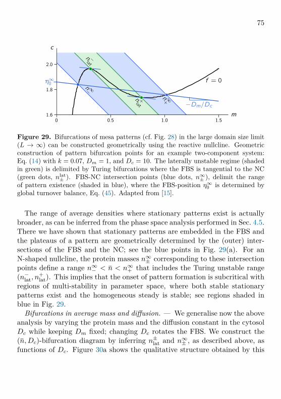
75

1.60 1.5

2.0

c

m0.5 1.0

1.8

Figure 29. Bifurcations of mesa patterns (cf. Fig. 28) in the large domain size limit(L → ∞) can be constructed geometrically using the reactive nullcline. Geometricconstruction of pattern bifurcation points for an example two-component system:Eq. (14) with k = 0.07, Dm = 1, and Dc = 10. The laterally unstable regime (shadedin green) is delimited by Turing bifurcations where the FBS is tangential to the NC(green dots, nlat

± ). FBS-NC intersection points (blue dots, n∞± ), delimit the rangeof pattern existence (shaded in blue), where the FBS-position η∞0 is determined byglobal turnover balance, Eq. (45). Adapted from [15].

The range of average densities where stationary patterns exist is actuallybroader, as can be inferred from the phase space analysis performed in Sec. 4.5.There we have shown that stationary patterns are embedded in the FBS andthe plateaus of a pattern are geometrically determined by the (outer) inter-sections of the FBS and the NC; see the blue points in Fig. 29(a). For anN-shaped nullcline, the protein masses n∞± corresponding to these intersectionpoints define a range n∞− < n < n∞+ that includes the Turing unstable range(n−lat, n

+lat). This implies that the onset of pattern formation is subcritical with

regions of multi-stability in parameter space, where both stable stationarypatterns exist and the homogeneous steady is stable; see regions shaded inblue in Fig. 29.

Bifurcations in average mass and diffusion. — We generalise now the aboveanalysis by varying the protein mass and the diffusion constant in the cytosolDc while keeping Dm fixed; changing Dc rotates the FBS. We construct the(n,Dc)-bifurcation diagram by inferring n±lat and n∞± , as described above, asfunctions of Dc. Figure 30a shows the qualitative structure obtained by this

76

(b)(a)

Figure 30. (n,Dc)-bifurcation diagram of stationary patterns for a system withmonostable kinetics (same color code as in Fig. 29). (a) The bifurcation diagramfor a large system (L → ∞) is obtained by tracking the geometrically constructedbifurcation points n±lat and n∞± as Dc, and thus the slope and position of the FBS, arevaried (cf. Fig. 29). The onset of lateral instability (Turing bifurcation shown as greendash-dotted line) is generically subcritical since there exist stationary patterns outsidethe range of lateral instability (n−lat, n

+lat); in the blue regions, the system is multi-

stable (both the stationary patterns and the homogenous steady state are stable).The regime where patterns exist, delimited by n∞± emerges from the critical point(ninf, D

minc ) (red point). (b) This critical point corresponds to the inflection point

of the nullcline at ninf where the nullcline slope −fm/fc reaches its extremal valuesnc(ninf). This determines the minimal cytosolic diffusion Dmin

c = −Dm/snc(ninf) (cf.Eq. (51)). At Dmin

c , the plateaus’ scaffolds m± bifurcate in a supercritical pitchforkbifurcation from the nullcline inflection point minf (see inset). Adapted from [15].

graphical construction.As Dc is decreased, the flux balance subspace becomes steeper, and thus the

bifurcation points n±lat and n∞± start to converge (see Fig. 30; cf. Fig. 29). Theymeet in the inflection point of the reactive nullcline, ninf, where the nullclineslope snc(ninf) is extremal (∂nsnc|ninf = 0). The extremal nullcline slope at thenullcline inflection point determines the minimal cytosolic diffusion constant,

Dminc := Dm

−snc(ninf), (51)

above which there are three FBS–NC intersection points. When the ‘criti-

77

Exercise 10. Determine the bifurcation diagram of a two-componentMCRD system with reaction kinetics f =

(1/4 + m2) c−m as a function

of the total protein mass n and the ratio of diffusion constants Dc/Dm.Indicate the boundaries of the Turing unstable regime as well as theboundaries of the regime where stationary patterns exist. Find closedanalytical expressions for both boundaries in the vicinity of the criticalpoint where both boundaries touch, i.e. at the inflection point minf ofthe nullcline c∗(m) = m/(1/4 + m2). Before starting a formal mathe-matical analysis familiarize yourself with the system’s behavior using agraphical analysis in (m, c)-phase space.

cal’ point (ninf, Dminc ) is traversed in Dc -direction, the FBS–NC intersections

bifurcate in a (supercritical) pitchfork bifurcation; see Fig. 30(b). Since theFBS–NC intersection points m± are the scaffolds for the plateaus (in short:plateau scaffolds; cf. Fig. 28), this bifurcation at the critical point (ninf, D

minc ) is

a bifurcation of the scaffold itself. Importantly, the actual pattern is boundedby the plateau scaffolds. Thus, if there are no plateau scaffolds (i.e. only oneFBS-NC intersection point), there cannot be stationary patterns. For L→∞,patterns emerge slaved to the plateau scaffold, such that the pattern bifurca-tion is supercritical at the nullcline inflection point (n = ninf). Away fromthe nullcline inflection point (n 6= ninf), the lateral instability bifurcation isalways subcritical for L→∞ because the range (n∞− , n∞+ ) where patterns existalways exceeds the range (n−lat, n

+lat) of lateral instability, as we learned above

(cf. Fig. 29).For clarity and simplicity we have confined the above analysis to the large

system size limit. As shown in [15] using weakly nonlinear analysis, for finiteL, the bifurcation is actually supercritical in the vicinity of the nullcline inflec-tion point. The transition from super- to sub-criticality depends on a subtleinterplay of diffusive and reactive flow.

Strikingly, our geometric reasoning shows that the physics implied by thebifurcation diagram is the same as in phase separation kinetics (binodal andspinodal regimes) for all N-shaped nullclines, and far away from the criticalpoint. This includes also cases where a mathematical equivalence of the under-

78

lying dynamics (e.g. in terms of a mapping to gradient dynamics) has not yetbeen found. This suggests that there might be a deeper connection betweentwo-component MCRD systems and phase separation kinetics near thermalequilibrium.

5 The role of bulk-boundary coupling for membranepatterns

The dynamics of most intracellular pattern forming systems involves a cou-pling between dynamics on the membrane surface and in the cytosolic volume(bulk). We exemplified this in Sec. 2.1 for the Min-protein dynamics, wherebiochemical interactions (with the exception of nucleotide exchange) are con-fined to the immediate vicinity of the membrane. At first glance, one mighttherefore suppose that it is straightforward to eliminate the cytosolic bulkfrom the dynamics and consider it simply as a passive particle reservoir. Al-though there are certain limits where this is indeed possible, in general, thebulk dynamics plays a key role for the spatiotemporal dynamics and can notbe disregarded. In the following we will illustrate the underlying physics fortwo simple analytically tractable cases, and discuss general implications forreaction–diffusion systems with bulk–boundary coupling. Moreover, we willdiscuss the implications of this coupling for the linear stability analysis andexplicitly show how such an analysis can be implemented for a box geome-try. Finally, in the last section we discuss how cytosolic gradients impact theformation of patterns and show how they lead to to geometry-induced patternformation.

5.1 Elementary examples in column geometryThis subsection illustrates the relevance of cytosolic density gradients for thedynamics of reaction-diffusion systems that couple reactions on a membraneand in the cytosol (bulk) through attachment and detachment of proteins. Tosimplify the calculations and highlight the role of gradients normal to the mem-brane we consider a simplified one-dimensional geometry: a narrow ‘column’of height h, with a membrane ‘point’ at the bottom (z = 0) and a reflective

79

column

cytosol

membrane

z

x

Figure 31. Illustration of a box and column geometry. For a conceptualanalysis of mass-conserving reaction-diffusion systems it is instructive to consider arectangular box geometry with the membrane considered as a one-dimensional line(x) and the cytosol as a two-dimensional rectangular box with vertical dimensionz ∈ [0, h]. An even simpler geometry is a narrow column where the membrane isconsidered as a point and the cytosol as a line.

boundary at z = h. By laterally coupling such ‘columns’ one obtains a ‘boxgeometry’, with a one-dimensional membrane and a two-dimensional cytosolicvolume as illustrated in Fig. 31. This is a simple, prototypical geometry tostudy reaction–diffusion systems with bulk-boundary coupling.

The exchange of proteins between membrane and cytosol (through variouskinds of chemical reactions as discussed in Sec. 2.2) needs to be balanced bydiffusive fluxes in the cytosol, otherwise local mass conservation would be vio-lated. Hence, on these very general grounds, there must be spatial gradients inthe cytosolic protein density. In this section we will answer the following ques-tions: What determines the magnitude and spatial extent of these cytosolicgradients? Under what conditions are these gradients essential for understand-ing the reaction-diffusion dynamics and when can they be neglected? What, inparticular, is the role of nucleotide exchange in the cytosol and the detachmentand attachment kinetics at the membrane?

Protein attachment causes cytosolic gradients. We start with analyzingthe effect of protein exchange between membrane and cytosol on the densityprofile c(z, t) in the cytosol. To keep the analysis simple we consider a singleprotein species which diffuses in the cytosol

∂tc(z, t) = Dc ∂2zc(z, t) , (52)

80

and that can attach to the membrane with rate kon

∂tm(t) = kon c(0, t) , (53)

where m signifies the density (number) of the proteins on the membrane.To complete the dynamics, one needs to specify boundary conditions. Thedynamics on the membrane and in the cytosol are coupled such that the over-all protein density is conserved locally. This requires that at the membranethe diffusive flux of proteins in the cytosol, jdiff = −Dc ∂zc(z, t)|z=0, and thereactive flux of proteins from the cytosol to the membrane (due to proteinattachment), jon = −kon c(0, t), need to match:

−Dc∂zc(z, t)|z=0 = −kon c(0, t) . (54)

This ‘reactive’ boundary condition is also called a ‘Robin’ boundary condition(see Sec. 2.1). It implies that the protein flux from the cytosol to the membraneleads to a depletion zone of proteins in the cytosol close to the membrane, i.e. agradient in the cytosolic density. The length scale (diffusion length) on whichthe profile relaxes back to the bulk protein level can be read off (by simpledimensional analysis) from Eq. (54) as11

`on :=√Dc/kon .

These considerations generalise to more complex reaction kinetics, for exampleby including a detachment flux jdetach = koffm(t), and clearly show that anyreactive coupling between the cytosol and the membrane inevitably leads todensity gradients in the cytosol. The set of dynamic equations is completedby the non-flux (reflective) boundary condition at z = h:

Dc ∂zc|z=h = 0 . (55)

Under what conditions can one disregard cytosolic gradients? Before start-ing with a formal analysis let’s start with some heuristic argument: the diffu-sive dynamics normal to the reactive membrane can be neglected if the time

11 Please note that the on-rate kon has dimension length/time since the cytosolic proteindensity is a line density and the membrane protein ‘density’ is actually a protein number.

81

scale of cytosolic mixing, τdiff ∼ h2/Dc, is much smaller than the typical time aprotein suspended in the bulk needs to attach to the membrane, τon ∼ h/kon.This yields the condition

h� òn ,

Only if this condition is obeyed, cytosolic gradients can be disregarded andthe cytosol be considered as a well-mixed particle reservoir.

It is also instructive to show this with a formal analysis. We are looking fora dynamic equation for the spatial average of the cytosolic protein density

c(t) = 1h

∫ h

0dz c(z, t) .

One finds, combining the cytosolic diffusion equation, Eq. (52), with bothboundary conditions, Eq. (54) and (55):

∂tc(t) = −konhc(0, t) .

This reduces to an equation for the concentration at the membrane c0(t) :=c(0, t) only if one can approximate the average density by the density at themembrane, c0(t) ≈ c(t). Then one gets a closed equation for the cytosolicdensity on the membrane (equivalently, the average cytosolic density)

∂tc0(t) ≈ −konhc0(t) . (56)

This equation is solved by c0(t) = c0(0) e−t/τon , an exponentially decayingreservoir of cytosolic particles, where the relaxation time is given by

τon := h/kon .

This approximation requires the absence of significant gradients in the cytosoland is valid only if the penetration depth òn is much larger than the heighth of the column, h � òn. This can also be seen explicitly because the con-sidered linear reaction-diffusion system is exactly solvable by the separation

82

ansatz c(z, t) = T (t)Z(z). With the separation constant σ, one finds a set ofdecoupled linear equations

∂tT (t) = σ T (t) ,Dc∂

2zZ(z) = σ Z(z) ,

which are solved by the ansatz

T (t) = T (0) eσt ,Z(z) = Z(h) cos

(p(h− z)

),

This shows that the separation constant σ plays the role of a growth rate. Wehave chosen the spatial part Z(z) such that it already respects the reflectiveboundary condition at z = h, Eq. (55). The wavenumber p is connected tothe growth rate σ via the dispersion relation

σp = −Dc p2 .

The possible values of p are determined by the reactive boundary conditionEq. (54), which upon substitution of the above ansatz yields

hp tan(hp) = h

òn. (57)

This type of transcendental equation makes the analysis of linear problemswith reactive boundary conditions coupling two compartments more involvedthan boundary value problems with reflective or Dirichlet boundary condi-tions.

Closed form solutions to the characteristic equation (57) exist in asymptoticlimits only. For h � òn, one can approximate tan(hp) ≈ hp to find thesmallest eigenvalue as p1 ≈ 1/

√hòn. Using the relation σp = −Dc p

2 fromabove, the corresponding relaxation rate is τ1 = 1/|σ1| turns out to be identicalto τon defined above.

After the decay of initial transients, corresponding to faster decaying smallerwavelengths, the dominant wavelength is

λmax = 2πp1

= 2π√hòn .

83

Since h � lon, one has λmax � 2πh, such that gradients on the scale of thecolumn can be neglected on time scales comparable and larger than τon. Onthat time scale, the dynamics of the longest wavelength mode then correspondsto the dynamics of the average cytosolic concentration, Eq. (56), c(z, t) ∝e−t/τ1 cos(p1(h − z)); note that cos(p1(h − z)) hardly shows any dependenceon the spatial coordinate z as p1 � h.

In the opposite limit of a large column height h � `on, the eigenvalues areapproximately given by pj ≈ (j−1/2)π/h with j ∈ N. Then, the largest wave-length λmax = 4h is comparable in size with column height h and gradients aresignificant. Hence, the cytosolic dynamics is an integral part of the system’sdynamics and can not effectively be described as some passive reservoir. Thereis an intricate interplay between protein dynamics in the vertically extendedcytosol and on the membrane.

A concrete biological example where this interplay plays an important roleis the Min system. The ‘bulk height’ in the cell geometry, given by the cellradius of approximately 0.5 µm, is magnitudes of order smaller than the typicalbulk heights from tens to several hundreds of micrometers in most in vitrosetups [38, 74–78]. This suggests that the bulk height is a key parameter thatdistinguishes the two scenarios and is responsible for the qualitative differencein phenomenology between in vivo and in vitro. Indeed, qualitatively differentmechanisms underlie pattern formation in these two regimes [79]. Pole-to-poleoscillations in cells and the patterns found at low bulk height (in the rangeof 1–5 µm) in the reconstituted system are driven by the same lateral mass-redistribution instability. In contrast, at large bulk heights the local equilibriacan become locally unstable. This oscillatory local instability is a consequenceof the extended bulk volume, where the bulk far away from the membraneeffectively acts as a reservoir that facilitates the local oscillations. In Sec. 6.2,we discuss how the local instabilities, triggered by lateral mass redistribution,play a key role for the Min pattern formation at large bulk heights.

Nucleotide exchange causes cytosolic gradients. Another important fac-tor that limits the elimination of cytosolic protein dynamics is nucleotide ex-change. As explained in Sec. 2.2, NTPases can switch between active (NTP-bound) and inactive (NDP-bound) states. The chemical reaction turning in-

84

active into active states is called nucleotide exchange. For instance, in the Minsystem, after MinE-cyatalyzed MinD-hydrolysis, MinD is released into the cy-tosol in its ADP-bound form. Reactivation by nucleotide exchange happensat a rate λ that is estimated to be λ ≈ 6 s−1; c.f. [18, 34]. Recently it hasbeen shown that even MinE shows switch-like behavior that is relevant for therobustness of pattern formation in the Min system [36].

Detachment of a protein from the membrane into the cytosol with a subse-quent change in conformation can be viewed as a ‘source-degradation’ process:the membrane acts as a MinD-ADP source, and nucleotide exchange corre-sponds to the ‘degradation’ process. This implies that the MinD-ADP densitydecays exponentially into the cytosol with a penetration depth given by thediffusion length

` :=√Dc/λ . (58)

Since typical values of the cytosolic diffusion constant Dc for proteins is invitro of the order Dc ≈ 60 µm2 s−1 [38], one estimates ` ≈ 3 µm, which is muchsmaller than typical system heights h used in in vitro experiments [38, 74]. Aswe will show next, these protein density gradients normal to the membranecritically influence the stationary density profiles at the membrane.

Consider again a one-dimensional column of height h with a simplified formof the MinD dynamics to illustrate the effect of nucleotide exchange in thebulk. The bulk dynamics of MinD-ATP and MinD-ADP are given by thereaction-diffusion equations

∂tcDD(z, t) = Dc ∂2zcDD − λ cDD , (59a)

∂tcDT(z, t) = Dc ∂2zcDT + λ cDD , (59b)

where cDD(z, t) and cDT(z, t) denote the cytosolic density of MinD-ADP andMinD-ATP, respectively. These are linear equations that can readily be solvedby a separation ansatz as above. In general, active MinD-ATP can bind to themembrane through some nonlinear attachment process, specified by a func-tion fon(m, cDT|z=0), that depends both on the density of membrane-boundMinD-ATP, m, and the cytosolic density of MinD-ATP close to the membranecDT|z=0. For simplicity, we do not model MinE explicitly but only effectivelythrough a detachment rate from MinD-ATP to cytosolic MinD-ADP specified

85

by the detachment rate koff. Then, the dynamics on the well-mixed membrane‘point’ reads

∂tm(t) = fon(m, cDT|z=0

)− koffm. (60)

At the membrane (z = 0), we use boundary conditions that reflect local massconservation: the diffusive fluxes for each protein state (active and inactive)have to match the corresponding reactive fluxes between membrane and cy-tosol:

−Dc ∂zcDD∣∣z=0 = koffm, (61a)

−Dc ∂zcDT∣∣z=0 = −fon

(m, cDT|z=0

). (61b)

In addition, we assume reflective boundary conditions at z = h:

Dc ∂zcDD∣∣z=h = 0 ,

Dc ∂zcDT∣∣z=h = 0 .

While the above analysis can be carried through for the full time-dependentproblem, we now focus on the analysis of the steady state. Then the setof stationary diffusion equations reads `2 ∂2

zcDD,DT = ∓cDD and, using thereflective boundary conditions at z = h, is solved by

c∗DD(z) = c∗DD,0cosh((h− z)/`)

cosh(h/`) , (62a)

c∗DT(z) = c∗DT,0 + c∗DD,0

(1− cosh ((h− z)/`)

cosh (h/`)

), (62b)

Note that the total cytosolic density of MinD is spatially uniform: c∗D(z) =c∗DD(z) + c∗DT(z) = const. As shown in Fig. 32, the MinD-ADP concentra-tion cDD(z) has its largest value at the membrane and then decays expo-nentially into the bulk where it saturates at c∗DD,0/ cosh(h/`). In contrast,the MinD-ATP concentration increases from c∗DT,0 to the saturation valuec∗DT,0 + c∗DD,0[1−1/ cosh(h/`)]. Hence, active MinD — the state of MinD thatcan attach to the membrane — is depleted close to the membrane and reachesits saturation value only at a distance ` away from the membrane. Takentogether this shows that within a layer of size `, active MinD is depleted whileinactive MinD is enhanced with respect to their respective bulk values.

86

z

h0

cDD,DT

cDD + cDT

1

0

MinD-ADP

MinD-ATP

Figure 32. Illustration of cytosolic density profiles of active and inactiveMinD. As one moves away from the membrane at z = 0, the density of inactive MinDis decreasing and the density of active MinD is increasing, mediated by nucleotideexchange, on a diffusive length scale ` =

√Dc/λ.

What determines the equilibrium protein concentrations (c∗DD,0, c∗DT,0, andm∗) at the membrane? It is the balance of the chemical reactions on themembrane, Eq. (60), local mass conservation, i.e. the matching between thereactive dynamics and diffusive fluxes at the membrane, Eq. (61), and globalmass conservation:

fon(m∗, c∗DT,0) = koffm∗ , (63a)

òff`

tanh (h/`) = m∗

c∗DD,0 òff, (63b)

c∗DT,0 + c∗DD,0 +m∗/h = n , (63c)

where we have defined a second diffusive length scale òff :=√Dc/koff, and n

signifies the mean total protein density.In the limit where the penetration depth ` is much smaller than the column

height, `�h, Eq. (63b) reduces to

òff`

= m∗

c∗DD,0 òff.

Since the total mass density n is an upper bounded for the bulk densities,n>cD,0, this implies that the stationary membrane density m∗ remains bound

87

from above in the limit h→∞

limh→∞

m∗ < n`2off`

= n

√Dcλ

koff.

Hence, one concludes that the combined effect of detachment kinetics andnucleotide exchange leads to a saturation effect for the membrane density,even in the absence of an explicit saturation term in the reaction kinetics.12

Notably, this emergent saturation effect only depends on the linear reactionkinetics but is completely independent of the attachment dynamics fon thatcould be highly cooperative. Moreover, this also limits the stationary proteinflux onto the membrane fon(m, cDT,0) = koffm <

√Dcλn [37].

The saturation effect strictly requires the extended bulk dimension. Tosee this we consider the analogous set of reaction equations with reducedbulk dimension, obtained — as in our first example above — by assuminga spatially homogeneous cytosolic protein density. Then one finds for thespatially averaged cytosolic densities ci(t) = 1

h

∫ h0 dz ci(z, t)

∂tcDD(t) = koffm/h− λ cDD , (64a)∂tcDT(t) = −fon(m, cDT)/h+ λ cDD (64b)∂tm(t) = fon(m, cDT)− koffm, (64c)

For the stationary state, one obtains from Eq. (64a)

m∗ = hλ

koffc∗DD .

which is obviously unbounded (for any finite c∗DD) as h → ∞. Hence, forlarge bulk heights, mass-conserving diffusion-reaction systems with nucleotideexchange in the cytosol, prohibit a naive elimination of the cytosol. If, however,the bulk height is small compared to the reactivation length scale, h � `,

12 This emergent saturation effect explains the surprising observation that models using asimplified (unsaturated) recruitment term kdDmdcDT reproduce both the Min dynamicsin vivo as well as in vitro with essentially the same kinetic parameters — despite thefact that membrane densities in vitro are two orders of magnitude higher than in vivo.

88

one has tanh(h/`) ≈ h/` such that using Eq. (63b) the reactive boundaryconditions, Eqs. (61a) and (61b), for the stationary bulk profiles reduce to

−Dc∂zcDD∣∣z=0 = −λ c∗DD,0 h = −koffm

∗ ,

−Dc∂zcDT∣∣z=0 = λ c∗DD,0 h = fon(m∗, c∗DT) .

This set of boundary conditions are identical to the stationarity condition inthe reduced system obtained from Eqs. (64a) and (64b) by setting the lefthand sides to zero. In summary, nucleotide exchange, a generic feature of allNTPase reaction cycles, prohibits an elimination of the cytosol unless h� `.

For typical experimental setups studying the Min system in vitro one hash/` = O(103) [38]. Hence one is actually in the opposite limit h� ` where bulkdynamics is essential. Neglecting nucleotide exchange or reducing the bulkdimension if the condition h� ` is not met would be an invalid approximationas it misses the saturation of membrane attachment.

5.2 Linear stability analysis in box geometryLet us not turn to laterally extended systems with bulk-boundary couplingand perform a linear stability analysis. As we will see, there are two key dif-ferences to the linear stability analysis in one spatial dimension (see Sec. 4.1).First, there may be vertical gradients in the bulk in steady state even if themembrane concentrations are laterally uniform. This has to be taken into ac-count when calculating the laterally homogeneous steady state around whichthe dynamics is linearised for stability analysis. Second, the algebraic problemthat results by solving the linearised dynamics in terms of the spatial eigen-modes is no longer an eigenvalue problem. Instead, one obtains a solvabilitycondition (‘characteristic equation’) which must be solved to find the growthrates corresponding to each eigenmode. Above, we already encountered anelementary form of such a solvability condition in the linear stability analysisfor a single column (see Eq. (57)).

As a simple geometry, consider the box-geometry that is formed by later-ally coupling vertical bulk-columns, each with a membrane point at its bot-tom (Fig. 31). This captures the physics of laterally extended systems withbulk-boundary coupling but avoids the mathematical complexity of the lin-ear stability analysis in a more realistic geometry like an ellipsoid [18] or a

89

sphere [21, 80]. In the box geometry, we simply have the diffusion operators∇2 = (∂2

x + ∂2z ) in the bulk and ∇2

m = ∂2x on the membrane, and the gradient

operator along the membrane’s inward normal ∇⊥ = ∂z.

Two-component system. To illustrate the basic procedure of linear stabilityanalysis in bulk-surface coupled systems, we first consider a system with only asingle cytosolic component c(x, z, t) and a single membrane componentm(x, t).For simplicity, we consider purely diffusive bulk dynamics

∂tc(x, z, t) = Dc(∂2x + ∂2

z )c, (65)

together with the reactive boundary condition (cf. Eq. (5))

−Dc∂zc|z=0 = −f(m, c|z=0), (66)

and no-flux conditions ∂xc|x=0,L = ∂zc|z=h = 0 at the remaining boundaries.The membrane dynamics are

∂tm(x, t) = Dm∂2xm+ f(m, c|z=0), (67)

with reflective boundaries ∂xmx=0,L = 0. These dynamics conserve the averagemass

n = 1L · h

∫ L

0dxm(x, t) +

∫ L

0dx∫ h

0dz c(x, z, t) . (68)

Exercise 11. In the limit of small bulk height, map the dynamics inbox geometry, Eqs. (65)–(67) to a 1d description (‘line geometry’) byapproximating the cytosol concentration at the membrane by the verti-cal average c(x, z = 0, t) ≈ 〈c(x, z, t)〉z. Under which conditions is suchan approximation valid?

The starting point of a linear stability analysis is the computation of asteady state around which the system can be linearised. For systems in 1dgeometry we studied in Sec. 4.3, we considered the stability of a homogeneoussteady state. The analog to this in a box geometry is a steady state that isspatially uniform along the membrane (i.e., in the lateral direction). However,

90

as we have learned from the analysis of the columnar geometry above, thecorresponding cytosolic densities can have vertical gradients while they arelaterally homogenous.

Because homogeneity along the membrane implies ∂xci = 0 in the entirebulk, the vertical bulk profiles of a laterally homogeneous steady state canbe obtained by the same reasoning as in Sec. 5.1. In the case of purely dif-fusive bulk dynamics, Eq. (65), the steady state bulk profile is determinedby ∂2

zc∗(z) = 0 and therefore homogeneous also in the vertical direction,

c∗(z) = c∗0; a constant gradient is prohibited by the no-flux boundary con-dition at the box’s ceiling z = h). The laterally homogeneous steady state ofEqs. (65)–(67) is therefore simply determined by

f(m∗, c∗0) = 0 and c∗0 +m∗/h = n. (69)

The linearised dynamics of a small perturbation c(x, z, t) = c∗(z)+δc(x, z, t),m(x, t) = m∗ + δm(x, t) is given by

∂tδc(x, z, t) = Dc(∂2x + ∂2

z )δc , (70a)−Dc∂zδc|z=0 = −fmδm− fcδc|z=0 , (70b)∂tδm(x, t) = Dm∂

2xδm+ fmδm+ fcδc|z=0 , (70c)

with the usual convention fm,c = ∂m,cf |(m∗,c∗0). To solve these equations, welook for solutions of the form

δc(x, z, t) = δm eσt cos(qx)Z(z;σ, q) , (71a)δm(x, t) = δc eσt cos(qx) , (71b)

where we used separation of variables for x, z, and t, and anticipated thatFourier modes will diagonalize the Laplace operator in the lateral direction(along the membrane) as in 1d geometry; cf. Sec. 4.3. Our goal is to find pairs(q, σ) for which this ansatz solves the linearised dynamics Eq. (70). Rewrittenin the form σ(q) these pairs constitute the dispersion relation that informsabout the growth rate(s) σ of perturbations with lateral wavenumber q.

First, the vertical eigenmode profiles Z(z) are obtained by substituting theseparation ansatz into Eq. (70a)

σZ(z;σ, q) = Dc q2 Z(z;σ, q) +DcZ

′′(z;σ, q) , (72)

91

which is solved by

Z(z;σ, q) = cosh(√

q2 + σ/Dc (h− z))/

cosh(√

q2 + σ/Dc h

). (73)

With this, the linearised bulk-surface coupling and the membrane dynamicsbecome a set of linear algebraic equations which are conveniently written inmatrix form (

Dc Γ(σ, q)− fc −fmfc −σ − q2Dm + fm

)︸︷︷︸

=: L(σ, q)

(δcδm

)= 0 , (74)

with the bulk-surface coupling coefficient

Γ(σ, q) := ∂zZ(z = 0;σ, q) = −√q2 + σ/Dc tanh

(√q2 + σ/Dc h

).

Solutions to the Equation (74) exist only if the solvability condition (char-acteristic equation)

detL(σ(q), q

)= 0 (75)

is fulfilled. This is the analog to the characteristic equation Eq. (32) of theeigenvalue problem Eq. (31) in 1d geometry. Because Γ(σ, q) is not linear inσ (here, it is actually non-algebraic), the matrix equation Eq. (74) does notconstitute an eigenvalue problem, though. To determine the dispersion rela-tion σ(q), we solve the characteristic equation (75) numerically, using iterativemethods like Newton’s method. An implementation of the above analysis inMathematica — computing the laterally homogeneous steady state and its lin-ear stability — is provided in the repository https://github.com/f-brauns/reaction-diffusion-stability [81].

Note that Eq. (75), has infinitely many solutions σi(q) for each q, corre-sponding to the set of vertical bulk-eigenmodes which form basis functions forthe bulk perturbations. This was discussed in more detail for the elementaryexample of a simple attachment process from a cytosolic column to a mem-brane ‘point’ above; see the discussion below Eq. (57). In particular, it wasshown that bulk perturbations with short wavelength modulations quickly de-cay owing to fast cytosolic diffusion. Thus the respective eigenvalues have a

https://github.com/f-brauns/reaction-diffusion-stability


92

large and negative real part. For linear stability analysis, we are typically onlyinterested in the solution σi(q) with the largest real part, which indicates thestability of the respective lateral mode cos(qx).

For growth rates close to zero, more precisely |σ| � q2Dc, one can expandthe coupling coefficient Γ to linear order in σ. Then Eq. (74) becomes an(approximate) eigenvalue problem the solutions of which provide good ini-tial guesses for iterative (Newton) methods to solve the exact characteristicequation (75).

Exercise 12. Show that in the limit h→ 0, Eq. (74) maps to the eigen-value problem Eq. (31) of the two-component MCRD system in 1d ge-ometry. The result should agree with the linear stability analysis of theapproximate dynamics in 1d geometry obtained in Exercise 11.

Min skeleton model. As a practical and slightly more complex example, werepeat the calculation of laterally homogeneous steady states and their linearstability analysis for the Min skeleton model [18, 37, 79]. The procedure isanalogous to the two-component case above. Some slight modifications arerequired to account for the nucleotide exchange of MinD in the bulk.

To simplify the analysis, we rewrite the MinD bulk dynamics in terms ofthe total bulk density cD = cDD + cDT together with the density of inactiveMinD, cDD. Together, the cytosolic densities are c = (cD, cDD, cE) while themembrane densities are m = (md,mde) as before. With these new variables,the reactive bulk-boundary fluxes (cf. Eq. (6)) read

f(m, c) =

−(kD + kdDmd)(cD − cDD)kdemde

kdemde − kdEmdcE

,and the membrane reactions (cf. Eq. (4)) are given by

Rmem(m, c) =(

(kD + kdDmd)(cD − cDD)− kdEmdcEkdEmdcE − kdemde

).

93

The advantage of the new variables is that the bulk equations decouple

∂tcD(x, z, t) = Dc∇2cD ,

∂tcDD(x, z, t) = Dc∇2cDD − λcDD ,

∂tcE(x, z, t) = Dc∇2cE ,

which immediately yields that the bulk profiles of the laterally homogeneoussteady state are uniform for cD and cE: c∗D,E(z) = c∗D,E(0). The bulk profilefor cDD is given by

c∗DD(z) = c∗DD(0)cosh

((h− z)/`D

)cosh(h/`D) ,

where `D =√Dc/λ; cf. Eq. (62a). The steady state bulk concentrations at the

membrane c∗D,DD,E(0) and the membrane concentrations m∗d,de are determinedvia the reactive boundary conditions; cf. Eq. (6),

fD = 0 , fE = 0 ,

fDD = −Dc

`Dtanh(h/`D) ,

and the condition that the membrane reactions are balanced

Rmem = 0 .

Moreover, global mass conservation enforces

nD = c∗D(0) + (m∗d +m∗de)/h ,nE = c∗E +m∗de/h .

For linear stability analysis, we again consider perturbations c = c∗(z) +δc∗(x, z, t), m = m∗ + δm∗(x, t), with the separation ansatz Eq. (71). Thebulk eigenmode equations for δcD and δcE are identical to Eq. (72), while wehave to replace σ → σ + λ to account for the linear degradation term in thelinearised bulk dynamics of δcDD. The bulk eigenmodes are thus given by

ZD,E(σ, q) = Z(σ, q) , ZDD(σ, q) = Z(σ + λ, q) ,

94

with Z(σ, q) defined by Eq. (73). Substituting the separation ansatz with thesebulk eigenmodes into the linearised bulk-boundary coupling and membranedynamics (cf. Eqs. (6) and (4)), we obtain the matrix equation(

Dc Γ(σ, q)− fc −fmRmem

c −σ − q2Dm + Rmemm

)︸︷︷︸

=: L(σ, q)

(δcδm

)= 0 ,

with the bulk-surface coupling coefficient matrix

Γ(σ, q) = diag(Γ(σ, q),Γ(σ + λ, q),Γ(σ, q)

),

and the linearised reaction terms

fm,c := ∂m,cf∣∣(m∗,c∗|S) ,

Rmemm,c := ∂m,cRmem

∣∣(m∗,c∗|S) .

Analogously to the two-component system above, the dispersion relationis determined by the characteristic equation detL

(σ(q), q

)= 0, which can

be solved numerically. An implementation of this analysis in Mathematica isprovided in the public repository [81].

Exercise 13. As a further generalisation, repeat the linear stabilityanalysis for the extended Min model that includes the MinE switch [36].Explore how fast switching between two MinE states affects the regimeof instability in the (nD, nE) parameter plane. To that end, write aprogram to numerically determine the homogeneous steady states andsolve the characteristic equation for the growth rates σ(q). You can usethe implementation for the Min skeleton model, provided in the onlinerepository [81], as a starting point.

5.3 Pattern formation without a lateral instabilityThis section serves to illustrate the importance of bulk-boundary coupling byshowing that it can facilitate the formation of patterns even in the absence of

95

membranecytosol

Total membraneconcentration

low highmembrane

cytosol

MinD-ATP MinD-ADP

(a) (b)

hydrol

ysis

nucleotideexchange

Figure 33. Geometry-induced pattern formation by proteins cycling be-tween membrane-bound and cytosolic states. (a) Generic interaction networkof an ATPase, like MinD, that can attach to the membrane, detaches from the mem-brane after hydrolysis, and undergoes nucleotide exchange in the cytoplasm. Self-recruitment (indicated by dashed arrows) enhances the geometry sensing but is notessential. (b) Nucleotide exchange in the cytosol with rate λ results in a layer of depth` =

√Dc/λ in which MinD-ADP is enriched. In regions where the radius of mem-

brane curvature is smaller than the penetration depth ` (illustrated by orange shad-ing), the MinD-ADP enrichment is enhanced due to the lower ratio of bulk-volume tomembrane-surface. This enhancement translates to increased (resp. decreased) mem-brane concentration in regions of high curvature if the membrane attachment of MinDis stronger (resp. weaker) in the ADP-bound state compared to the ATP-bound state.

any lateral instability [82]. To this end, we consider a basic reaction modulethat comprises a single type of NTPase which cycles between a NDP-boundand a NTP-bound state; see Fig. 33a. It is assumed that both protein confor-mations can attach to the membrane either directly with rates k+

D and k+T , or

cooperatively by forming homo-dimers with corresponding recruitment rateskdD and ktT for the NDP- and the NTP-bound state, respectively. Membrane-bound, inactive proteins can detach into the cytosol with detachment rate k−d ,while active proteins detach only after hydrolysis with rate k−t . In the cytosol,inactive proteins are transformed into active ones by nucleotide exchange withrate λ. As discussed in [82], this reaction network serves as a model for thebipolar pattern of AtMinD in E. coli cells [83].

In elliptical geometry, as illustrated in Fig. 33b, this reaction module is

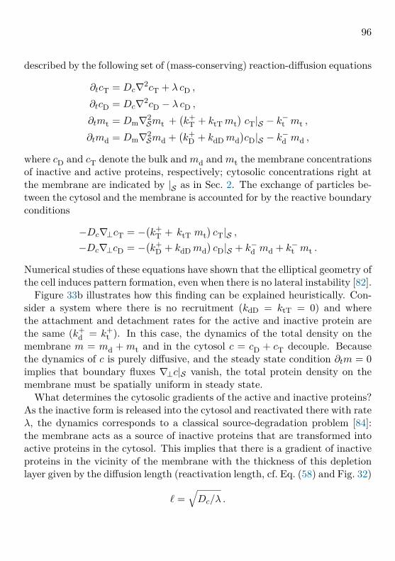
96

described by the following set of (mass-conserving) reaction-diffusion equations

∂tcT = Dc∇2cT + λ cD ,

∂tcD = Dc∇2cD − λ cD ,

∂tmt = Dm∇2Smt +

(k+

T + ktTmt)cT|S − k−t mt ,

∂tmd = Dm∇2Smd +

(k+

D + kdDmd)cD|S − k−d md ,

where cD and cT denote the bulk and md and mt the membrane concentrationsof inactive and active proteins, respectively; cytosolic concentrations right atthe membrane are indicated by |S as in Sec. 2. The exchange of particles be-tween the cytosol and the membrane is accounted for by the reactive boundaryconditions

−Dc∇⊥cT = −(k+

T + ktT mt)cT|S ,

−Dc∇⊥cD = −(k+

D + kdDmd)cD|S + k−d md + k−t mt .

Numerical studies of these equations have shown that the elliptical geometry ofthe cell induces pattern formation, even when there is no lateral instability [82].

Figure 33b illustrates how this finding can be explained heuristically. Con-sider a system where there is no recruitment (kdD = ktT = 0) and wherethe attachment and detachment rates for the active and inactive protein arethe same (k+

d = k+t ). In this case, the dynamics of the total density on the

membrane m = md + mt and in the cytosol c = cD + cT decouple. Becausethe dynamics of c is purely diffusive, and the steady state condition ∂tm = 0implies that boundary fluxes ∇⊥c|S vanish, the total protein density on themembrane must be spatially uniform in steady state.

What determines the cytosolic gradients of the active and inactive proteins?As the inactive form is released into the cytosol and reactivated there with rateλ, the dynamics corresponds to a classical source-degradation problem [84]:the membrane acts as a source of inactive proteins that are transformed intoactive proteins in the cytosol. This implies that there is a gradient of inactiveproteins in the vicinity of the membrane with the thickness of this depletionlayer given by the diffusion length (reactivation length, cf. Eq. (58) and Fig. 32)

` =√Dc/λ .

97

Since these gradients overlap at the cell poles, one expects an increased con-centration of inactive proteins there; for an illustration see Fig. 33b. Themagnitude of this effect depends on the ratio of this diffusion length withrespect to the cell length L, and should vanish as ` � L. These argumentsexplain why the local ratio of the reaction volume for nucleotide exchange (cy-tosolic volume) to the available membrane surface facilitates geometry-inducedpattern formation.

To gain a deeper conceptual understanding of these heuristic results it isinstructive to map the spatially extended model onto a system with a set ofdiscretized nodes (Fig. 34a). The idea of the mapping is that the placementand number of nodes is chosen such that it faithfully accounts for the differentratios of membrane area to bulk volume at the cell poles and at mid-cell.Due to the elliptical symmetry, this system can be further reduced to onequadrant of the ellipse, leaving one with a network of one membrane nodeat a pole and one at mid-cell, two nodes representing the interface betweenmembrane and cytosol, and three cytosolic nodes. The corresponding set ofordinary differential equations can be found in the Supplementary Materialof [82]. Solving these equations leads to two main insights: First, the simpleNTPase model indeed leads to polarisation between cell pole and mid-cell,corresponding to a bipolar pattern in the whole cell (Fig. 34b). Second, onecan perform a standard bifurcation analysis which shows that the steady statesdo not undergo any bifurcation. One finds only one physically possible solutionwith positive protein density on the membrane and this density increases withrecruitment rate.13 This implies that the reaction module exhibits a robustmechanism for geometry-induced pattern formation amplified by nonlinearfeedback but without an underlying Turing instability.

13 Only in the limiting (non-generic) case where the attachment rate of inactive proteinvanishes, does one find a transcritical bifurcation. Hence one concludes, that a geneticNTPase reaction module shown in Fig. 33a generically has an imperfect transcriticalbifurcation.

98

PNDP

membrane border cytosol

mid-cellpole

membraneborder

0.11

0.02

(a)

(b)

Figure 34. Spatial domain reduction to set of nodes. (a) The dynamics ofa spatially extended system, described in terms of partial differential equations, canbe approximately reduced to a set of ordinary differential equations describing thedynamics on a network of coupled nodes. The nodes are considered as well mixedand diffusion corresponds to exchange of proteins between these nodes. The set ofnodes is chosen such that it approximately represent the bulk-to-surface ratio at thecell poles and at midcell. Here, we only consider symmetric stationary states, suchthat we only need to consider a single quadrant explicitly. (b) Illustration of thereduced model with two membrane nodes at the pole and at mid-cell, two bordernodes connecting membrane and cytosol, as well as three cytosolic nodes. Note thatthe top-right cytosolic node (dark blue) accounts for the increased ratio of membranearea to bulk volume at mid-cell. This network of nodes polarises with the color of thenodes indicating the density of inactive proteins PNDP.

99

6 Control space dynamics6.1 The control space conceptConsider a multi-component, mass-conserving reaction-diffusion (MCRD) sys-tem as discussed in section 2.3. It is described in terms of the densities of allthe components (states of protein species) in the biochemical reaction networkui(x, t) with i ∈ {1, . . . , N}. In general, the number N of these components islarge compared to the number S of protein species with mass densities nα(x, t)where α ∈ {1, . . . , S}; see the reaction networks shown in Fig. 2. How can onereduce the complexity of such large multi-component systems?

From the analysis of two-component MCRD systems in Section 4 we gainedthe following key insights. Pattern formation is mainly driven by the spa-tiotemporal dynamics of protein masses. While the average values for eachprotein mass nα are fixed by mass conservation, their local values nα(x, t)are in general spatially inhomogeneous and can change over time. Dynamicsof protein masses inevitably leads to moving local equilibria since at a givenspatial location x (and given time t) the value of the fixed point (equilibrium)u∗i (x, t) of the underlying biochemical network is determined by the corre-

charaterizationand classificationin control spacelocal stability

concentration gradients mass transport

local equilibria

Figure 35. Conceptualization of MCRD dynamics. Deneralisation of thescheme shown in Fig. 26, to an arbitrary number of components ci and conservedmasses nα. In addition to moving, i.e. changing position in phase space, the localequilibria c∗i can also change their stability as indicated by the leading local eigenvalueσloc. The information about the position and stability of local equilibria as a functionof the masses nα is encoded in the bifurcation structure in control space; see Fig. 36for an example.

100

sponding set of local values for the protein masses: u∗i (x, t) = u∗i ({nα(x, t)}).In other words, the local protein masses act as dynamic control variables, incontrast to the reaction rates of the biochemical network that are global andfixed control parameters. These local equilibria drive local reactive fluxes thatchange the gradients in the densities of the various components of the proteinnetwork, which in turn drive diffusive fluxes that lead to a redistribution ofprotein masses (Fig. 26). This suggests that the essential dynamics of a multi-component system should be captured already in terms of the local densitiesof the conserved protein masses. We will refer to the space spanned by thesecontrol variables as control space; for an illustration see Fig. 35.

In that control space it is straightforward to perform a linear stability anal-ysis of both the local and lateral stability of the spatially homogeneous state.Figure 36 illustrates the result of such a bifurcation analysis for a system withtwo conserved protein species with mass densities n1 and n2. The regionsshaded in red and green show the domains of local and lateral stability, re-spectively. The lilac spot indicates the average masses n1 and n2 of the twoprotein species. Imagine now that the spatially extended system is dissectedinto a set of small (well-mixed) compartments which are represented as pointsin control space. While for a spatially uniform state all of these points arecondensed into the point corresponding to the average protein densities, theybecome spread out in phase space as soon as there is a spatially heterogeneousdistribution of protein masses.

In Fig. 36, the average mass densities n1 and n2 are chosen such that it liesin a domain of lateral instability but local stability; see lilac point in Fig. 36.Hence, any small perturbation of a spatially uniform state will lead to a patternthat initially is dominated by the wavelength (in the band of unstable modes)with the largest (positive) eigenvalue. In control space this implies that the setof phase space points representing the spatially extended system form a cloudwith a center of mass given by the phase space point marking the spatiallyhomogeneous state. As the amplitude of the pattern grows, there are twodistinct scenarios. Either, the amplitude of the pattern (deviation of the localmasses from the average masses) stays bounded and remains in the domain oflocal stability (Fig. 36, left), or the amplitude becomes so large that eventuallythe dynamics becomes locally unstable in some of the compartments (Fig. 36,

101

locally unstable

stable

laterally unstable

locally unstable

stable

laterally unstable

Figure 36. Concept of control space. Performing a linear stability analysis of aspatially extended system (using the proper eigenmodes for the geometry under con-sideration) one finds domains in control space (n1, n2) which are locally unstable (redregion) or laterally unstable (green region). Starting from a spatially homogeneoussystem in a domain of lateral instability but local stability (lilac point correspondingto average masses (n1, n2)) there are two distinct scenarios: Either the amplitude ofthe patterns stays bounded and the system does not enter the domain of local insta-bility (left, supercritical case), or the amplitude grows large and enters the domain oflocal instability (right, subcritical case).

right). The first case is typical for a supercritical instability, where uponapproaching the onset of instability the amplitude of the pattern continuouslygoes to zero. In contrast, for a subcritical system, the amplitude of the patterngrows to large amplitude even at onset. Hence, it does not remain boundedin a small domain of control space but may extend into the regime of localinstability. This can lead to a complex spatiotemporal dynamics, as we willillustrate in the next section for the specific example of the Min system.

6.2 Control space attractors of the in vitro Min systemWe illustrate the control space concept for the Min system in box geome-try, which is frequently used in experimental studies of the reconstituted Minsystem on supported lipid bilayers [36, 38, 74–78, 85]. The spiral patterns

102

observed in experiments are reproduced by numerical simulations of the Minskeleton model as discussed in Section 2.3, see Fig. 6. The membrane is lo-cated at the bottom of the box and the height h of the bulk volume is used asa control parameter.

For simplicity we consider a two-dimensional slice geometry with the mem-brane given by a line of finite length L and the bulk (cytosol) as a slice withthe same length L and height h; see Fig. 6. For the Min system there aretwo globally conserved chemical species, MinD and MinE, with local densitiesnD(x, z, t) and nE(x, z, t), respectively. We define the local total densities inthe immediate vicinity of the membrane (z = 0), normalised with respect totheir time-independent spatial averages as

D(x, t) = nD(x, z = 0, t)nD

,

E(x, t) = nE(x, z = 0, t)nE

.

The total densities right at the membrane, rather than, for instance, theirvertical averages, are the proper control variables, because only these densitiesparticipate in the nonlinear dynamics at the membrane at each instant t. Fordetails on this so called ‘adiabatic extrapolation’ please refer to [37].

As coordinates in the control space spanned by the total densities, we usethe local MinD-MinE ratio

∆(x, t) := E(x, t)/D(x, t)

and the local root mean-square sum of protein densities Σ(x, t), defined as

Σ(x, t) := 1√2

(E2(x, t) +D2(x, t)

)1/2.

For specificity, we choose the Min skeleton model aas the reaction scheme(Fig. 2), resulting in the set of dynamic equations specified in Section 2.3;the parameters for the reaction rates, diffusion constants, and the averageprotein densities are given in Table 1. Performing a linear stability analysiswith respect to a spatially homogeneous state in box geometry [37, 79], oneobtains a stability diagram in control space that contains domains of local

103

0 2

1.3

0.9

1

1

(a) (b)

0.003

0.60locally unstable

laterally unstable

stable

Figure 37. Linear stability analysis of the Min system. (a) Stability diagramin the parameter space of total densities of MinD and MinE, parametrized by Σ and ∆(defined in text). Note that the ratio of MinE to MinD mass, ∆, is the key parameter,while Σ is almost irrelevant. (b) Dispersion relation at the point (Σ,∆) = (1, 1), whichlies very close to the onset of lateral instability. (Bulk height h = 20 µm, remainingparameters as in Table 1.)

and lateral instability. Figure 37a shows the stability diagram obtained forh = 20 µm which is chosen such that the spatially homogeneous state is slightlyabove the rim of lateral instability. The corresponding dispersion relation(for the real part of the largest eigenvalue), shown in Fig. 37b, exhibits anarrow band of unstable modes, where q denotes the wave vector in lateraldirection x. This dispersion relation implies that a spatially homogeneous stateis (barely) unstable and initially a periodic pattern will form with a wavelengthdetermined by the fastest growing mode. However, it does not inform us aboutthe ensuing spatiotemporal dynamics far away from the homogeneous steadystate.

To learn about the nature of these highly nonlinear dynamics, we followthe dynamics both in real space and in control space starting from a slightlyperturbed, homogeneous steady state, similar as for the two-component sys-tem. Snapshots of the control space distribution at four different time pointstogether with a spatiotemporal ‘waterfall plot’ of the MinD membrane densityare shown in Fig. 39. The control space plots show the euclidean distance Astate

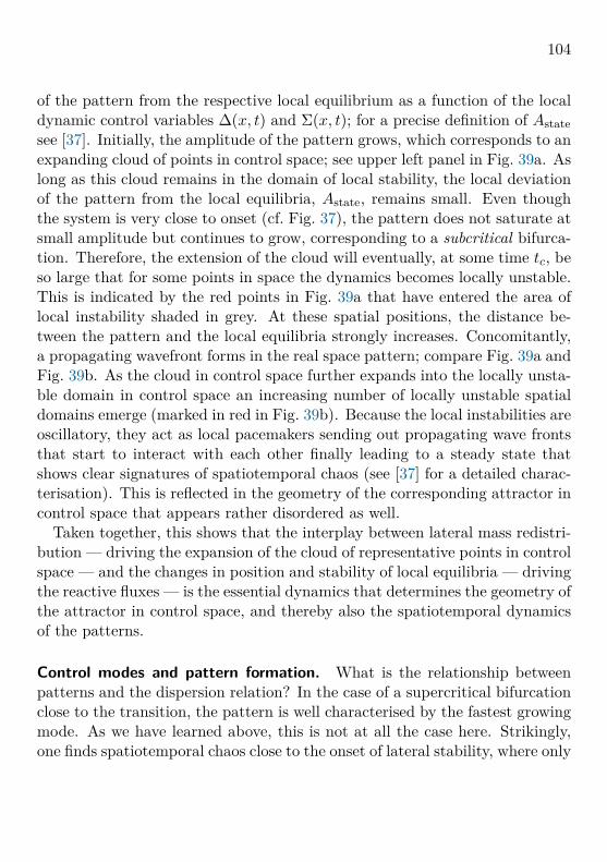
104

of the pattern from the respective local equilibrium as a function of the localdynamic control variables ∆(x, t) and Σ(x, t); for a precise definition of Astatesee [37]. Initially, the amplitude of the pattern grows, which corresponds to anexpanding cloud of points in control space; see upper left panel in Fig. 39a. Aslong as this cloud remains in the domain of local stability, the local deviationof the pattern from the local equilibria, Astate, remains small. Even thoughthe system is very close to onset (cf. Fig. 37), the pattern does not saturate atsmall amplitude but continues to grow, corresponding to a subcritical bifurca-tion. Therefore, the extension of the cloud will eventually, at some time tc, beso large that for some points in space the dynamics becomes locally unstable.This is indicated by the red points in Fig. 39a that have entered the area oflocal instability shaded in grey. At these spatial positions, the distance be-tween the pattern and the local equilibria strongly increases. Concomitantly,a propagating wavefront forms in the real space pattern; compare Fig. 39a andFig. 39b. As the cloud in control space further expands into the locally unsta-ble domain in control space an increasing number of locally unstable spatialdomains emerge (marked in red in Fig. 39b). Because the local instabilities areoscillatory, they act as local pacemakers sending out propagating wave frontsthat start to interact with each other finally leading to a steady state thatshows clear signatures of spatiotemporal chaos (see [37] for a detailed charac-terisation). This is reflected in the geometry of the corresponding attractor incontrol space that appears rather disordered as well.

Taken together, this shows that the interplay between lateral mass redistri-bution — driving the expansion of the cloud of representative points in controlspace — and the changes in position and stability of local equilibria — drivingthe reactive fluxes — is the essential dynamics that determines the geometry ofthe attractor in control space, and thereby also the spatiotemporal dynamicsof the patterns.

Control modes and pattern formation. What is the relationship betweenpatterns and the dispersion relation? In the case of a supercritical bifurcationclose to the transition, the pattern is well characterised by the fastest growingmode. As we have learned above, this is not at all the case here. Strikingly,one finds spatiotemporal chaos close to the onset of lateral stability, where only

105

(a) (b) (c)

Figure 38. Illustration of the dispersion relation as a function of bulkheight. At h = hSW, the right edge of the band of unstable modes (unstable modewith the shortest wavelength), qmax, becomes commensurate with the fastest growingmode qc.

very few modes are unstable. Generally, patterns emerging from a subcriticalbifurcation cannot be characterised in terms of the dispersion relation alone.However, a systematic numerical study of the dynamics as one increases thebifurcation parameter h shows that there is a remarkable relation between thedispersion relation and the observed pattern.

Upon increasing the height, one observes a transition from turbulence-like patterns to spatially coherent standing wave patterns, at threshold valuehSW≈ 23.5 µm. This transition coincides precisely with the point where theunstable mode qmax with the shortest wavelength (right side of the band ofunstable modes) becomes commensurable with the critical (fastest growing)mode qc: qmax = 2qc; see Fig. 38. Increasing the height even further, both thecritical mode qc and its commensurate mode qr = 2qc < qmax are linearly un-stable and one observes travelling waves. Heuristically, this can be explainedas the coordinated interplay of the fastest growing mode qc, which controls thedistribution of wave sources and sinks by triggering local instabilities, and itscommensurate mode qr which drives the mass-redistribution between the wavenodes [37]. However, a systematic understanding of this route from chaos toorder and the associated commensurability criterion remains elusive. The roleof the local instabilities that act as pacemakers and are periodically triggeredby lateral mass redistribution suggests that the local oscillatory instability isa key requirement.

In control space, the transition between patterns is reflected in a change in

106

the type of attractor (Fig. 40). The control-space attractor corresponding tothe turbulence-like state for h < hSW has no discernible structure. Standingwaves undergo amplitude modulations on large spatial scales. Therefore thedistribution in control space appears as a broad band. In contrast to thecontrol attractor corresponding to chemical turbulence, the standing waveattractor is highly ordered. The spatial and temporal periodicity of travelingwaves is reflected in a collapse of the control space distribution onto a singleclosed orbit, which corresponds to the cycle traversed by the concentrationsat each point in space during one wave period.

The prediction of turbulence-like dynamics at the onset of lateral instabil-ity and coherent patterns deeper in the unstable regime has recently beenconfirmed in experiments with the in vitro Min system [36]. Moreover, lo-cal oscillations of the Min proteins between membrane and bulk have beenobserved in vesicles (radius ∼ 10 µm) [86, 87]. Together, these experimen-tal findings suggest that the mechanisms identified by the theoretical analysisindeed underlie the dynamics in the experimental system.

107

Fig

ure

39.

Tim

eev

olut

ion

ofa

chao

tic

patt

ern

inco

ntro

lspa

ce.

(a)S

naps

hots

ofth

eco

ntro

lspa

cedi

strib

utio

nat

four

times

.St

artin

gfro

ma

near

lyho

mog

eneo

usin

itial

stat

e(i.

e.a

poin

tin

cont

rols

pace

),th

edi

strib

utio

nex

pand

sdr

iven

byla

tera

lins

tabi

lity

alon

eun

til,a

ta

timet c

,it

star

tsto

ente

rth

ere

gim

eof

loca

lins

tabi

lity

(top

right

pane

l).In

the

loca

llyun

stab

lere

gim

e(s

hade

din

grey

),th

epa

tter

nis

driv

enaw

ayfro

mth

elo

cale

quili

bria

resu

lting

ina

stro

ngin

crea

seinA

stat

e.(b

)Spa

tiote

mpo

ralw

ater

fall

plot

ofth

eM

inD

mem

bran

ede

nsity

.R

edpo

ints

mar

klo

catio

nsw

here

the

loca

lequ

ilibr

ium

isun

stab

le.

(Par

amet

ersa

sin

Fig.

37;a

dapt

edfro

m[3

7].)

108

0

1.5

0

1.2

0

1.0

Chem

ical t

urbu

lence

Stan

ding

wav

eTr

aveli

ng w

ave

Fig

ure

40.

Snap

shot

sof

the

dens

itypr

ofile

san

dth

eco

rres

pond

ing

cont

rols

pace

dist

ribut

ions

ofth

ein

vitr

oM

insy

stem

with

bulk

heig

htsh

=21,3

0,an

d35

µm,f

rom

left

torig

ht;

rem

aini

ngpa

ram

eter

sas

inTa

ble

1.T

here

gim

eof

loca

lins

tabi

lity

issh

aded

inre

din

the

cont

rols

pace

plot

s.N

ote

how

the

incr

easin

gsp

atia

lcoh

eren

cein

the

patt

ern

profi

les

isre

flect

edin

anin

crea

sein

orde

ran

dde

crea

sein

dim

ensio

nalit

yof

the

cont

rols

pace

attr

acto

rs.

109

7 Conclusions and OutlookIn this final section we will not only give an overview of the theoretical con-cepts that we introduced, but also provide an outlook on open questions. Theconclusions will summarise generic design aspects of protein-interaction net-works for pattern formation, and emphasise the overarching ideas underlyingthe theoretical analysis of the mathematical models describing such systems:MCRD equations. In a nutshell this theory includes the local reactive concept,the mechanism of the mass-redistribution instability, a flux-balance construc-tion in the phase plane of the reaction kinetics, and the control space concept.In addition, we briefly discuss the consequences of cytosolic gradients nor-mal to the membrane that arise generically from the bulk-boundary couplingbetween cytosol and membrane.

In the outlook we will discuss some recent ideas on how to apply and gen-eralise the theory of MCRD systems. In the context of (conceptual) two-component systems, we discuss forthcoming works on the question of lengthscale selection (coarsening), the role of cytosolic flow, the role of heterogene-ity in the spatial domain serving as a ‘template’, and the role of a verticallyextended cytosol. Moreover, we give a perspective on the generalisation oflocal equilibria theory beyond two-component models and strict mass con-servation, focussing on the topics of model classification and model reduc-tion. Finally we propose to revisit classical pattern-forming systems like theBelousov–Zhabotinsky reaction, treating them as nearly mass conserving sys-tems.

7.1 ConclusionsGeneric design of pattern-forming protein networks. The reaction-diffusionequations describing the spatiotemporal dynamics of proteins in cells exhibitseveral characteristic features:

• The underlying biochemical reaction networks have one or several NTP-ase cycles as core modules. These cycles consume free energy by con-verting NTP to NDP thereby breaking detailed balance such that thedynamics is genuinely non–equilibrium in nature. Additional key ele-ments of the reaction networks include proteins that activate and deac-

110

tivate the NTPases, termed NEFs and NAPs, as well as various types offeedback mechanisms.

• On the timescale of pattern formation and maintenance, protein produc-tion and degradation that break the conservation of mass for each proteinspecies are typically negligible. Hence protein dynamics is described bymass-conserving reaction–diffusion equations. Production and degrada-tion of proteins slowly change the average protein masses that play therole of control parameters for these dynamics.

• The proteins diffuse on the membrane and in the cytosol, i.e. on a two-dimensional closed surface and in a three-dimensional confined bulk vol-ume. Most chemical reactions are confined to the membrane, whilethe cytosol mainly serves as a (spatially non-uniform) particle reser-voir. Chemical reactions in the cytosol are largely linear processes likenucleotide exchange such that the reaction–diffusion equations in thecytosol can be solved in closed form using eigenfunctions of the diffusion(Laplace) operator appropriate for the particular cell geometry.

• The diffusion constant for proteins in the membrane and the cytosol dif-fer by orders of magnitude. While this is important for the quantitativeanalysis of a given system, the pattern formation mechanism that wediscussed only require that these diffusion constants are different.

• Proteins are exchanged between membrane and cytosol respecting localconservation of protein masses. Reactive fluxes between membrane andcytosol necessarily lead to spatial protein gradients in the cytosol. Due tothese gradients, the spatial geometry of the system (e.g. the cell shape)can play an essential role for the formation of patterns. This entailsthat the cytosol can, in general, not be considered as a well-mixed par-ticle reservoir, but rather one has to account for its full spatiotemporaldynamics.

Phase-space geometry of nonlinear systems. The overarching idea in thedescription of nonlinear systems is their characterisation in terms of ‘geomet-ric structures’ in phase space, a key mathematical insight going back to the

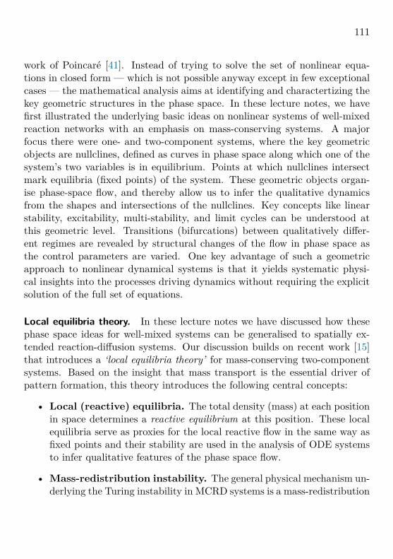
111

work of Poincare [41]. Instead of trying to solve the set of nonlinear equa-tions in closed form — which is not possible anyway except in few exceptionalcases — the mathematical analysis aims at identifying and charactertizing thekey geometric structures in the phase space. In these lecture notes, we havefirst illustrated the underlying basic ideas on nonlinear systems of well-mixedreaction networks with an emphasis on mass-conserving systems. A majorfocus there were one- and two-component systems, where the key geometricobjects are nullclines, defined as curves in phase space along which one of thesystem’s two variables is in equilibrium. Points at which nullclines intersectmark equilibria (fixed points) of the system. These geometric objects organ-ise phase-space flow, and thereby allow us to infer the qualitative dynamicsfrom the shapes and intersections of the nullclines. Key concepts like linearstability, excitability, multi-stability, and limit cycles can be understood atthis geometric level. Transitions (bifurcations) between qualitatively differ-ent regimes are revealed by structural changes of the flow in phase space asthe control parameters are varied. One key advantage of such a geometricapproach to nonlinear dynamical systems is that it yields systematic physi-cal insights into the processes driving dynamics without requiring the explicitsolution of the full set of equations.

Local equilibria theory. In these lecture notes we have discussed how thesephase space ideas for well-mixed systems can be generalised to spatially ex-tended reaction-diffusion systems. Our discussion builds on recent work [15]that introduces a ‘local equilibria theory’ for mass-conserving two-componentsystems. Based on the insight that mass transport is the essential driver ofpattern formation, this theory introduces the following central concepts:

• Local (reactive) equilibria. The total density (mass) at each positionin space determines a reactive equilibrium at this position. These localequilibria serve as proxies for the local reactive flow in the same way asfixed points and their stability are used in the analysis of ODE systemsto infer qualitative features of the phase space flow.

• Mass-redistribution instability. The general physical mechanism un-derlying the Turing instability in MCRD systems is a mass-redistribution

112

instability. It is based on a feedback loop between lateral redistributionof mass and moving local equilibria. As local masses change, the lo-cal equilibria shift, thus driving the formation of gradients, which inturn lead to further redistribution of mass. In two-component MCRDsystems, the condition for this instability can be phrased as a simplegeometric criterion: negative slope of the reactive nullcline in the phase-portrait of the reaction kinetics. generalising the mechanism of a mass-redistribution instability beyond reaction–diffusion systems reveals ananalogy between a Turing instability and Ostwald ripening [88].

• Diffusive flux balance. In a stationary pattern, the diffusive fluxeson the membrane and in the cytosol have to balance at each position inspace. This condition implies that a stationary pattern must lie in anaffine subspace (i.e. a straight line) in phase space.

• Flux-balance construction. Combining the concepts of local equilib-ria and diffusive flux balance enables one to construct stationary patterns(and their bifurcation diagrams) in the phase portrait of the reaction ki-netics. This construction can be pictured as an analog to the Maxwellconstruction (also known as ‘common tangent construction’ [89]) used tofind the equilibrium phases in the phase separation of binary mixtures.

• Concept of regions. In general, patterns can be understood as con-sisting of distinct spatial regions (e.g. plateaus with high/low density,interfaces, etc.), which correspond to different regions in phase space.This general idea can be employed to rigorously derive specific propertiesof the pattern, like the interface width and the threshold perturbationfor stimulus-induced pattern formation, from the geometric phase-spaceanalysis. For a more in-depth analysis of this idea we refer the interestedreader to [15].

• Control variables and control space. Total densities play the roleof control parameters for the local reactive dynamics while they are vari-ables of the spatially extended system. We therefore refer to them ascontrol variables and introduce the control space, which is the phasespace spanned by the control variables. The control space and the bifur-

113

cation structure in it (obtained by linear stability analysis) can be usedto characterise and classify the MCRD dynamics.

Bulk-boundary coupling. A general property of intracellular protein patternsis the coupling between protein dynamics on the membrane and protein dy-namics in the cytosol. There is an exchange of proteins between both compart-ments due to linear and cooperative attachment and detachment processes. Animmediate consequence of this coupling is the existence of protein gradients inthe cytosol, whose extent depends on the cytosolic diffusion constant as well ason some characteristic rates for the exchange of proteins between membraneand cytosol or the reactivation of proteins in the cytosol (Sec. 5). For exam-ple, nucleotide exchange in the bulk leads to depletion zones of active proteinswithin a layer of size ` =

√Dc/λ. These cytosolic gradients are responsible

for the geometry dependence of the ensuing protein patterns [82, 90, 91]. Areduced description in terms of surface variables (membrane concentrationsand cytosolic concentrations at the membrane) by elimination of the cytoso-lic dynamics normal to the membrane is possible only if the diffusion lengthcorresponding to the gradients is much larger than the size of a cell or theheight of a microfluidic device in vitro [79]. Finally, we introduced the basicelements of linear stability analysis for systems with bulk-boundary couplingwhich complicates the linear stability analysis of the laterally homogeneoussteady states (Sec. 5.2). The key step there is to find a common set of spatialeigenmodes that diagonalises the diffusion operator on the membrane, in thecytosol, and in the bulk-boundary coupling simultaneously. These eigenmodesthen play an analogous role to the Fourier modes in the classical linear stabilityanalysis of one-dimensional systems.

Dynamics in control space. The control space concept can be used to char-acterise and to rationalise numerically obtained dynamics as we demonstratedin Sec. 6.2 for the in vitro Min system. There, we have summarised the find-ings of recent papers [36, 37, 79]. The analysis in control space reveals thatthe lateral redistribution of mass locally triggers destabilisation of the localequilibria. This local destabilisation is responsible for the development of spa-tiotemporal chaos close to the onset of lateral instability. This prediction from

114

numerical simulations has recently been confirmed in experiments [36]. Fur-ther away from onset, standing and travelling waves emerge from an interplaybetween commensurable ‘control modes’ that synchronise the points in timeand space where local instabilities are triggered. A systematic understandingof this route from spatiotemporal chaos to order remains elusive. Nonetheless,the progress made so far demonstrates how the control space concept helps tobridge the gap between linear stability analysis and highly nonlinear dynamicsfar away from the homogeneous steady state.

The Min system. Throughout these lecture notes, the Min system of E. colihas served as a paradigmatic example for protein-based pattern formation.This reflects the important role of the Min system in the field, both for exper-imental and theoretical research on intracellular pattern formation; see e.g.[23] and references cited therein. A major experimental milestone was thereconstitution of the Min system in vitro by [38]. These experiments clearlydemonstrated, that only two proteins, MinE and MinD, and chemical fuel inthe form of ATP are required for pattern formation on a lipid bilayer thatmimics the cell membrane. This reconstitution provides a minimal systemthat enables precise control of reaction parameters and geometrical constrains[36, 38, 74–78, 85, 86, 92–94]. These studies show that, despite its molecularsimplicity, the Min system exhibits a remarkable variety of phenomena.

The rich phenomenology of the Min system, and the relative simplicityof its protein-interaction network, also make it an ideal testing ground fortheoretical ideas such as the control space analysis [36, 37] and the role of cellgeometry [18, 90, 95]. In addition, upon engineering the interaction networkby modifying the protein domains one can address the relevance of specificprocesses in the reaction network for the ability of the system to robustlyform patterns [36] and design minimal pattern-forming systems [85].

Despite the significant progress there still remain several important openquestions. First, the precise biomolecular mechanism underlying MinD’s self-recruitment still remains elusive. A possible mechanism based on indirectmechano-chemical interactions has recently been suggested by [96] but has yetto be tested experimentally. Second, there are striking differences betweenthe dynamics in cells and in reconstituted systems, both qualitatively (pole-

115

to-pole- and stripe-oscillations vs. spiral waves, uniform oscillations, quasi-stationary patterns, etc.) and quantitatively concerning the characteristiclength- and timescales of the patterns. In a forthcoming publication, we willaddress this long standing puzzle and show that the ratio of bulk-volume tosurface-area (i.e. the bulk height) is the key parameter that distinguishes thein vivo regime from classical in vitro setups [79]. A characterisation of thedynamics in control space shows that there is no local instability at low bulkheights, such that patterns are driven by lateral instabilities alone. Localinstabilities only come into play at sufficiently large bulk heights, where theygive rise to the phenomena characteristic for the in vitro system, as discussedin Sec. 6.2. A third open question is the mechanism underlying the quasi-stationary patterns observed in recent experiments using reconstituted MinEwith the purification tag removed [78]. Further extensions of the skeletonmodel [17, 18] may be required to account for this phenomenon.

The future looks bright! With new advances in microfluidics and proteinchemistry, we expect the Min system as well as other reconstituted proteinsystems to even gain importance as model systems for testing new theoreticalideas on self-organisation in biological systems. In particular, these systemswill be instrumental in further extending and generalising the ideas and con-cepts presented in these lecture notes and our recent publications [15, 37].

7.2 OutlookTwo-component MCRD systems were instrumental in developing general phasespace concepts like the flux-balance subspace and the physics of the under-lying pattern forming mechanism, namely the mass-redistribution instability.These systems have also been instrumental in identifying the total proteinmass and the mass-redistribution potential as key quantities for a conceptualunderstanding of the mechanisms driving pattern formation and leading tothe formation of stationary states. However, there still remain a series ofopen questions. These include the coarsening dynamics, the role of hetero-geneities in the spatial domain that act as ‘templates’ or ‘pre-patterns’ andcytoplasmic advective flows, and generalisations that explicitly take into ac-count the extended bulk and the accompanying reactive boundary conditions(bulk-boundary coupling).

116

Coarsening in two-component models. While we now have a rather com-plete understanding of the instability mechanism and the final polar patternof two-component MCRD systems, the mechanism responsible for the coars-ening process from an initially periodic pattern towards the polar patternremains elusive. The discussion in Sec. 4.5, where we introduced the mass-redistribution potential hints towards a possible solution. Indeed, coarseningcan be understood as a mass-redistribution instability driven by gradients inthe mass-redistribution potential between spatial regions, each containing anelementary pattern (a single ‘peak’ or ‘mesa’) [73]. Using elementary geo-metric arguments that build on the phase-portrait analysis presented here,we show that uninterrupted coarsening is indeed generic in two-componentreaction–diffusion systems with mass conservation [73].

The question of coarsening is a particular case of the more general problemof length-scale selection far away from the homogeneous steady state. In ourview, this is one of the key open challenges in the field. Previous attemptsto find a general theory remain restricted to one-component systems [97, 98].Our analysis of two-component MCRD systems shows that the spatial redis-tribution of globally conserved quantities plays a key role in the coarseningdynamics. Combining mathematical tools like multi-scale analysis, renormal-isation group theory, and singular perturbation theory with the physical con-cepts of local equilibria theory a new approach to coarsening dynamics has tobe developed that can be generalised to multi-component systems.

Cytoplasmic advective flows. Cytoplasmic advective flows play an impor-tant role in cellular systems [99–101]. The influence of bulk flow on protein-based pattern formation has also been studied in the reconstituted Min system[74, 76]. Conceptually this can be studied by straightforward generalisation ofthe two-component system discussed in Sec. 4, illustrated in Fig. 41a, namelyby adding an advection term to the cytosolic dynamics:

∂tc(x, t) + v ∂xc(x, t) = Dc∂2xc(x, t) + f(m, c) . (76)

How does this affect the formation of patterns? Does this induce moving pat-terns and how is the direction of pattern motion correlated with the directionof cytoplasmic flow? In [102], these questions are addressed using the concepts

117

membrane

cytosol(a) (b)

membrane

cytosol advective flow

steplike template

Figure 41. Illustration of two-component MCRD systems with cytoplasmic advec-tive flow (a) and with a steplike spatial template (b).

of local equilibria theory [15, 37] discussed in Sec. 4. In particular, it is shownthat in two-component systems, cytoplasmic flow generically induces motionof high-density regions upstream (i.e. against the flow direction). In contrast,preliminary results indicate that systems with more components exhibit bothupstream and downstream propagation in response to cytoplasmic flow. Thedirection of propagation induced by the flow is found to depend sensitivelyon the underlying protein-interaction network, suggesting that externally im-posed flows can be used to probe the molecular details of pattern-formingsystems in experiments.

Patterns forming patterns. In his seminal paper on reaction-diffusion sys-tems Turing pointed out [11] that “most of an organism, most of the time,is developing from one pattern into another, rather than from homogeneityinto a pattern.” While it is not fully clear what he was referring to with thisstatement, there are several biological scenarios for such a hierarchy or se-quence of patterns. In one scenario, previously formed protein patterns canacts as a spatial template for the formation of subsequent protein patterns byaffecting their local reaction kinetics. A more intriguing scenario is a fullyself-organised temporal sequence of protein patterns with increasing complex-ity, as recently observed in starfish ooctyes [48]. Another striking exampleof this is the morphogenesis of the drosophila embryo, where the positionalinformation provided by the (maternal) bicoid gradient is precisely read outand translated into a complex gene expression pattern via a hierarchy of generegulatory circuits [103]. While, patterns in drosophila appear to be highly

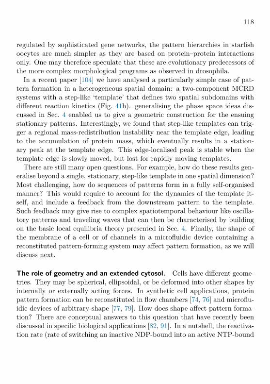
118

regulated by sophisticated gene networks, the pattern hierarchies in starfishoocytes are much simpler as they are based on protein–protein interactionsonly. One may therefore speculate that these are evolutionary predecessors ofthe more complex morphological programs as observed in drosophila.

In a recent paper [104] we have analysed a particularly simple case of pat-tern formation in a heterogeneous spatial domain: a two-component MCRDsystems with a step-like ‘template’ that defines two spatial subdomains withdifferent reaction kinetics (Fig. 41b). generalising the phase space ideas dis-cussed in Sec. 4 enabled us to give a geometric construction for the ensuingstationary patterns. Interestingly, we found that step-like templates can trig-ger a regional mass-redistribution instability near the template edge, leadingto the accumulation of protein mass, which eventually results in a station-ary peak at the template edge. This edge-localised peak is stable when thetemplate edge is slowly moved, but lost for rapidly moving templates.

There are still many open questions. For example, how do these results gen-eralise beyond a single, stationary, step-like template in one spatial dimension?Most challenging, how do sequences of patterns form in a fully self-organisedmanner? This would require to account for the dynamics of the template it-self, and include a feedback from the downstream pattern to the template.Such feedback may give rise to complex spatiotemporal behaviour like oscilla-tory patterns and traveling waves that can then be characterised by buildingon the basic local equilibria theory presented in Sec. 4. Finally, the shape ofthe membrane of a cell or of channels in a microfluidic device containing areconstituted pattern-forming system may affect pattern formation, as we willdiscuss next.

The role of geometry and an extended cytosol. Cells have different geome-tries. They may be spherical, ellipsoidal, or be deformed into other shapes byinternally or externally acting forces. In synthetic cell applications, proteinpattern formation can be reconstituted in flow chambers [74, 76] and microflu-idic devices of arbitrary shape [77, 79]. How does shape affect pattern forma-tion? There are conceptual answers to this question that have recently beendiscussed in specific biological applications [82, 91]. In a nutshell, the reactiva-tion rate (rate of switching an inactive NDP-bound into an active NTP-bound

119

state) defines a depletion zone of active NTPases close to the membrane; seeSec. 5.1. It will then depend on the local ratio of membrane surface to cytoso-lic volume how likely proteins of the different conformations reencounter themembrane, which affects pattern formation. How can one formalise this heuris-tic argument such that the local equilibria theory can be used to study patternformation? This requires to extend the techniques explained in Sec. 4 to ex-plicitly account for an extended cytosolic volume and the reactive couplingbetween membrane and cytosol; cf. Sec. 5. Is it possible to find a reductionscheme that eliminates the extended cytosol and reduces the reaction-diffusiondynamics to an effectively one-dimensional system? What are the conditionsfor such a reduction scheme to work? Preliminary studies indicate that it is ac-tually possible to answer these questions informing about the role of geometryand bulk-boundary coupling for MCRD systems [105, 106]. In this context, itis the geometry induced spatial distribution of masses that drives or inhibitspattern formation. As another distinct mechanism, a mechano-chemical feed-back between biochemical reaction networks and the shape of the surroundinggeometry can lead to a variety of complex dynamics [96].

Model classification and reduction One of the key insights underlyinglocal equilibria theory is that mass-redistribution is the key driver of the dy-namics. In other words, total densities are the essential degrees of freedom.This provides a new perspective for model reduction and the classification ofpattern forming systems.

For instance, it has been suggested that the generic bifurcation scenario forcell polarity is a cusp bifurcation [60]. In fact we were recently able to showthat patterns in two-component MCRD systems — which are the conceptualand elementary case for polar pattern formation — generically unfolds from acusp bifurcation [15]. This bifurcation scenario generally arises for N-shapedreactive nullclines (or, more generally, nullclines with a section of negativeslope), which are necessary and sufficient for pattern formation in theses sys-tems.

More complex phenomenology can arise in multi-component models withmore than one conserved quantity — such that the control space becomesmulti-dimensional — and/or due to more complex bifurcation scenarios in

120

control space. The Min system encompasses both these scenarios. The pole-to-pole oscillations in vivo arise due to mass redistribution of MinE betweenthe cell poles, periodically switching the direction of MinD polarisation. Im-portantly, the local equilibria remain stable at all times during this oscillationcycle. This allows one to map the in vivo Min-protein dynamics to relaxationoscillations in the two-dimensional control space by generalising the principleof scaffolding by local equilibria [107]. The much richer phenomenology of thereconstituted Min system (in vitro) emerges as a consequence of a more com-plex bifurcation scenario in control space, involving the destabilisation of localequilibria in Hopf bifurcations that give rise to local limit cycle oscillations (cf.Sec. 6.2). Motivated by these results, we anticipate that new model reductionapproaches and a systematic classification scheme for MCRD systems can bederived based on the dynamics and bifurcation scenarios in control space.

Beyond strict mass conservation: revisiting classical systems. The classof nearly mass-conserving reaction–diffusion systems comprises many widelystudied (classical) pattern-forming systems, including the Belusov–Zhabotinsky(BZ) reaction [108, 109], oxidation of carbon monoxide on platinum surfaces(short PtCO system) [110, 111], and intracellular calcium (Ca2+) oscillations[112, 113]. It is likely that each of these systems exhibits a mass-conservingcore, meaning that their capability to form patterns and key features of thesepatterns are captured by a mass-conserving subset of their reaction kinetics.This makes these systems potentially amenable to local equilibria theory andthe tools and concepts presented in Sec. 4 and Sec. 6. The reactions breakingmass-conservation may then be treated as perturbations to the core systemthat modify the patterns.

As an example, take the Brusselator model, which can be rewritten as amass-conserving two-component system (its ‘core’), perturbed by a constantproduction and a linear degradation term (cf. Eq. (27)). Pattern formationis driven by a mass-redistribution instability of the core system, and the sta-tionary patterns of the core system can be constructed by the phase-portraitanalysis presented in Sec. 4. The production and degradation terms perturbthese core patterns on large length- and timescales. In particular, they inter-rupt the coarsening process at a finite length scale [114, 115]. Applying this

121

approach to more classical pattern-forming systems is an exiting perspectivefor future research and might provide a deeper understanding of their richphenomenology.

Acknowledgements. We would like to thank all of our collaborators thatover the years have shaped our understanding of pattern formation in bio-logical systems, especially Silke Bergeler, Jonas Denk, Raphaela Geßele, An-driy Goychuk, Jacob Halatek, Tobias Hermann, Ben Klunder, Ching Yee Le-ung, Tobias Reichenbach, Steffen Rulands, Dominik Thalmeier, Henrik Weyer,Manon Wigbers, Laeschkir Wurthner, and Alexander Ziepke. Without themit would have been impossible to get to the state of writing lecture notes onthis topic. Our special thanks also goes to our experimental collaborationpartners from the laboratories of Cees Dekker, Nikta Fakhri, Liedewij Laan,and Petra Schwille. They are a continuous source of stimulation and inspira-tion for our theoretical work. Finally, we would like to gratefully acknowledgefinancial support from the Deutsche Forschungsgemeinschaft (DFG, GermanResearch Foundation).

References[1] G. Laloux and C. Jacobs-Wagner. How do bacteria localize proteins

to the cell pole? Journal of Cell Science, 127(1):11–19, 2013. doi:10.1242/jcs.138628.

[2] L. Shapiro, H. H. McAdams, and R. Losick. Why and how bacterialocalize proteins. Science, 326(5957):1225–1228, 2009. doi: 10.1126/science.1175685.

[3] P. A. de Boer, R. E. Crossley, and L. I. Rothfield. A division inhibitor anda topological specificity factor coded for by the minicell locus determineproper placement of the division septum in e. coli. Cell, 56(4):641–649,1989. doi: 10.1016/0092-8674(89)90586-2.

[4] D. M. Raskin and P. A. J. de Boer. Rapid pole-to-pole oscillation of aprotein required for directing division to the middle of escherichia coli.

122

Proceedings of the National Academy of Sciences, 96(9):4971–4976, 1999.doi: 10.1073/pnas.96.9.4971.

[5] B. E. Walker, J. Mannik, and J. Mannik. Transient membrane-linked ftszassemblies precede z-ring formation in escherichia coli. Current Biology,30(3):499–508.e6, 2020. doi: 10.1016/j.cub.2019.12.023.

[6] H. P. Erickson, D. E. Anderson, and M. Osawa. FtsZ in bacte-rial cytokinesis: Cytoskeleton and force generator all in one. Mi-crobiology and Molecular Biology Reviews, 74(4):504–528, 2010. doi:10.1128/mmbr.00021-10.

[7] B. Alberts, A. Johnson, J. Lewis, M. Raff, K. Roberts, and P. Walter.Molecular Biology of the Cell. Garland Science, New York, 5th edition,2007.

[8] R. Phillips. Physical Biology of the Cell. Garland Science, London :New York, NY, 2nd edition, 2013. ISBN 978-0-8153-4450-6.

[9] D. D. Leipe, Y. I. Wolf, E. V. Koonin, and L. Aravind. Classification andevolution of p-loop gtpases and related atpases. Journal of MolecularBiology, 317(1):41–72, 2002. doi: 10.1006/jmbi.2001.5378.

[10] R. Thom. Structural Stability And Morphogenesis. Addison-Wesley,1975. Translated from the French edition by D. H. Fowler.

[11] A. M. Turing. The chemical basis of morphogenesis. Philosophical Trans-actions of the Royal Society B: Biological Sciences, 237(641):37–72, 1952.doi: 10.1098/rstb.1952.0012.

[12] J. Guckenheimer and P. Holmes. Nonlinear Oscillations, Dynamical Sys-tems, and Bifurcations of Vector Fields. Number 42 in Applied Mathe-matical Sciences. Springer, New York, 1983.

[13] M. Cross and H. Greenside. Pattern Formation and Dynamics inNonequilibrium Systems. Cambridge University Press, 2009.

123

[14] J. D. Murray. Mathematical Biology II: Spatial Models and Biomed-ical Applications, volume 17 of Interdisciplinary Applied Mathematics.Springer, New York, 3 edition, 2003. ISBN 0-387-95228-4.

[15] F. Brauns, J. Halatek, and E. Frey. Phase-Space Geometry of Mass-Conserving Reaction-Diffusion Dynamics. Physical Review X, 10(4):041036, 2020. doi: 10.1103/PhysRevX.10.041036.

[16] J. Lutkenhaus. Assembly dynamics of the bacterial MinCDE system andspatial regulation of the Z ring. Annual Review of Biochemistry, 76(1):539–562, 2007. doi: 10.1146/annurev.biochem.75.103004.142652.

[17] K. C. Huang, Y. Meir, and N. S. Wingreen. Dynamic structures inescherichia coli: Spontaneous formation of mine rings and mind polarzones. Proceedings of the National Academy of Sciences, 100(22):12724–12728, 2003. doi: 10.1073/pnas.2135445100.

[18] J. Halatek and E. Frey. Highly canalized MinD transfer and MinE se-questration explain the origin of robust MinCDE-protein dynamics. CellReports, 1(6):741–752, 2012. doi: 10.1016/j.celrep.2012.04.005.

[19] E. Bi and H.-O. Park. Cell polarization and cytokinesis in budding yeast.Genetics, 191(2):347–387, 2012. doi: 10.1534/genetics.111.132886.

[20] T. Freisinger, B. Klunder, J. Johnson, N. Muller, G. Pichler, G. Beck,M. Costanzo, C. Boone, R. A. Cerione, and E. Frey. Establishmentof a robust single axis of cell polarity by coupling multiple positivefeedback loops. Nature Communications, 4(1):1807 PE, 2013. doi:10.1038/ncomms2795.

[21] B. Klunder, T. Freisinger, R. Wedlich-Soldner, and E. Frey. GDI-mediated cell polarization in yeast provides precise spatial and tem-poral control of Cdc42 signaling. PLoS Computational Biology, 9(12):e1003396, 2013. doi: 10.1371/journal.pcbi.1003396.

[22] N. W. Goehring, P. K. Trong, J. S. Bois, D. Chowdhury, E. M. Nicola,A. A. Hyman, and S. W. Grill. Polarization of PAR proteins by advective

124

triggering of a pattern-forming system. Science, 334(6059):1137–1141,2011. doi: 10.1126/science.1208619.

[23] J. Halatek, F. Brauns, and E. Frey. Self-organization principles of in-tracellular pattern formation. Philosophical Transactions of the RoyalSociety B: Biological Sciences, 373(1747):20170107, 2018. doi: 10.1098/rstb.2017.0107.

[24] D. I. Johnson. Cdc42: An essential Rho-type GTPase controlling eu-karyotic cell polarity. Microbiol Mol Biol Rev, 63(1):54–105, 1999.

[25] J. Chant and I. Herskowitz. Genetic control of bud site selection in yeastby a set of gene products that constitute a morphogenetic pathway. Cell,65(7):1203–12, 1991.

[26] G. Koch, K. Tanaka, T. Masuda, W. Yamochi, H. Nonaka, and Y. Takai.Association of the rho family small GTP-binding proteins with Rho GDPdissociation inhibitor (Rho GDI) in saccharomyces cerevisiae. Oncogene,15(4):417–22, 1997. doi: 10.1038/sj.onc.1201194.

[27] J. L. Johnson, J. W. Erickson, and R. A. Cerione. New insights intohow the rho guanine nucleotide dissociation inhibitor regulates the in-teraction of Cdc42 with membranes. Journal of Biological Chemistry,284(35):23860–23871, 2009. doi: 10.1074/jbc.m109.031815.

[28] I. Bose, J. E. Irazoqui, J. J. Moskow, E. S. Bardes, T. R. Zyla, and D. J.Lew. Assembly of scaffold-mediated complexes containing Cdc42p, theexchange factor Cdc24p, and the effector Cla4p required for cell cycle-regulated phosphorylation of Cdc24p. J. Biol. Chem., 276(10):7176–86,2001.

[29] A.-C. Butty, N. Perrinjaquet, A. Petit, M. Jaquenoud, J. E. Segall,K. Hofmann, C. Zwahlen, and M. Peter. A positive feedback loop stabi-lizes the guanine-nucleotide exchange factor Cdc24 at sites of polariza-tion. EMBO J., 21(7):1565–76, 2002.

125

[30] J. E. Irazoqui, A. S. Gladfelter, and D. J. Lew. Scaffold-mediated sym-metry breaking by Cdc42p. Nature Cell Biology, 5(12):1062–1070, 2003.doi: 10.1038/ncb1068.

[31] C. Hoege and A. A. Hyman. Principles of par polarity in caenorhabditiselegans embryos. Nature Reviews Molecular Cell Biology, 14(5):315–322,2013. doi: 10.1038/nrm3558.

[32] E. Munro, J. Nance, and J. R. Priess. Cortical flows powered by asym-metrical contraction transport PAR proteins to establish and maintainanterior–posterior polarity in the early C. elegans embryo. Developmen-tal Cell, 7(3):413–424, 2004. doi: 10.1016/j.devcel.2004.08.001.

[33] F. O. Bendezu, V. Vincenzetti, D. Vavylonis, R. Wyss, H. Vogel, andS. G. Martin. Spontaneous Cdc42 polarization independent of GDI-mediated extraction and actin-based trafficking. PLOS Biology, 13(4):e1002097, 2015. doi: 10.1371/journal.pbio.1002097.

[34] G. Meacci, J. Ries, E. Fischer-Friedrich, N. Kahya, P. Schwille, andK. Kruse. Mobility of Min-proteins in escherichia coli measured by fluo-rescence correlation spectroscopy. Physical Biology, 3(4):255–263, 2006.doi: 10.1088/1478-3975/3/4/003.

[35] E. Frey, J. Halatek, S. Kretschmer, and P. Schwille. Protein Pattern For-mation, pages 229–260. Springer International Publishing, 2018. ISBN9783030006303. doi: 10.1007/978-3-030-00630-3 10.

[36] J. Denk, S. Kretschmer, J. Halatek, C. Hartl, P. Schwille, and E. Frey.MinE conformational switching confers robustness on self-organized Minprotein patterns. Proc. Natl. Acad. Sci. U.S.A., page 201719801, 2018.doi: 10.1073/pnas.1719801115.

[37] J. Halatek and E. Frey. Rethinking pattern formation in reaction–diffusion systems. Nature Physics, 14(5):507–514, 2018. doi: 10.1038/s41567-017-0040-5.

[38] M. Loose, E. Fischer-Friedrich, J. Ries, K. Kruse, and P. Schwille.Spatial regulators for bacterial cell division self-organize into surface

126

waves in vitro. Science, 320(5877):789–792, 2008. doi: 10.1126/science.1154413.

[39] S. H. Strogatz. Nonlinear Dynamics and Chaos. Westview Press, 2ndedition, 2014.

[40] E. M. Izhikevich. Dynamical systems in neuroscience: the geometry ofexcitability and bursting. The MIT Press, Cambridge, Massachusetts,2007. ISBN 978-0-262-09043-8.

[41] H. Poincare. Les methodes nouvelles de la mecanique celeste, volume 1–3. Gauthiers-Villars, Paris, 1892, 1893, 1899. English translation editedby D. Goroff, published by the American Institute of Physics, New York,1993.

[42] S. Wiggins. An Introduction to Applied Nonlinear Dynamical Systemsand Chaos. Springer, New York, 2nd edition, 2003.

[43] Y. Mori, A. Jilkine, and L. Edelstein-Keshet. Wave-pinning and cellpolarity from a bistable reaction-diffusion system. Biophysical Journal,94(9):3684–3697, 2008. doi: 10.1529/biophysj.107.120824.

[44] P. C. Hohenberg and B. I. Halperin. Theory of dynamic criticalphenomena. Reviews of Modern Physics, 49(3):435–479, 1977. doi:10.1103/revmodphys.49.435.

[45] J. E. Ferrell, T. Y.-C. Tsai, and Q. Yang. Modeling the cell cycle:Why do certain circuits oscillate? Cell, 144(6):874–885, 2011. doi:10.1016/j.cell.2011.03.006.

[46] B. Novak and J. J. Tyson. Design principles of biochemical oscillators.Nature Reviews Molecular Cell Biology, 9(12):981–991, 2008. doi: 10.1038/nrm2530.

[47] S. Etienne-Manneville and A. Hall. Rho GTPases in cell biology. Nature,420(6916):629–635, 2002.

127

[48] M. C. Wigbers, T. H. Tan, F. Brauns, Z. S. Schwartz, E. Frey, andN. Fakhri. A hierarchy of protein patterns robustly decodes cell shapeinformation. Accepted in Nature Physics, 2020.

[49] I. Prigogine and R. Lefever. Symmetry breaking instabilities in dissi-pative systems. ii. The Journal of Chemical Physics, 48(4):1695–1700,1968. doi: 10.1063/1.1668896.

[50] J. Schnakenberg. Simple chemical reaction systems with limit cycle be-haviour. Journal of Theoretical Biology, 81(3):389–400, 1979.

[51] A. Gierer and H. Meinhardt. A theory of biological pattern formation.Kybernetik, 12(1):30–39, 1972. doi: 10.1007/bf00289234.

[52] L. A. Segel and J. L. Jackson. Dissipative structure: An explanationand an ecological example. Journal of Theoretical Biology, 37(3):545–559, 1972. doi: 10.1016/0022-5193(72)90090-2.

[53] S. Ishihara, M. Otsuji, and A. Mochizuki. Transient and steady stateof mass-conserved reaction-diffusion systems. Phys. Rev. E, 75:015203,2007. doi: 10.1103/PhysRevE.75.015203.

[54] M. Otsuji, S. Ishihara, C. Co, K. Kaibuchi, A. Mochizuki, and S. Kuroda.A mass conserved reaction–diffusion system captures properties of cellpolarity. PLoS Computational Biology, 3(6):e108, 2007. doi: 10.1371/journal.pcbi.0030108.

[55] A. B. Goryachev and A. V. Pokhilko. Dynamics of Cdc42 network em-bodies a Turing-type mechanism of yeast cell polarity. FEBS Letters,582(10):1437–43, 2008. doi: 10.1016/j.febslet.2008.03.029.

[56] S. J. Altschuler, S. B. Angenent, Y. Wang, and L. F. Wu. On thespontaneous emergence of cell polarity. Nature, 454(7206):886–889, 2008.doi: 10.1038/nature07119.

[57] A. Jilkine and L. Edelstein-Keshet. A comparison of mathemati-cal models for polarization of single eukaryotic cells in response toguided cues. PLoS Computational Biology, 7(4):e1001121, 2011. doi:10.1371/journal.pcbi.1001121.

128

[58] A. Jilkine, S. B. Angenent, L. F. Wu, and S. J. Altschuler. A density-dependent switch drives stochastic clustering and polarization of signal-ing molecules. PLoS Computational Biology, 7(11):e1002271, 2011. doi:10.1371/journal.pcbi.1002271.

[59] L. Edelstein-Keshet, W. R. Holmes, M. Zajac, and M. Dutot. From sim-ple to detailed models for cell polarization. Philosophical Transactions ofthe Royal Society B: Biological Sciences, 368(1629):20130003–20130003,2013. doi: 10.1098/rstb.2013.0003.

[60] P. K. Trong, E. M. Nicola, N. W. Goehring, K. V. Kumar, and S. W.Grill. Parameter-space topology of models for cell polarity. New Journalof Physics, 16(6):065009, 2014. doi: 10.1088/1367-2630/16/6/065009.

[61] J.-G. Chiou, S. A. Ramirez, T. C. Elston, T. P. Witelski, D. G. Schaeffer,and D. J. Lew. Principles that govern competition or co-existence inRho-GTPase driven polarization. PLoS Computational Biology, 14(4):e1006095, 2018. doi: 10.1371/journal.pcbi.1006095.

[62] L. Hubatsch, F. Peglion, J. D. Reich, N. T. L. Rodrigues, N. Hirani,R. Illukkumbura, and N. W. Goehring. A cell-size threshold limits cellpolarity and asymmetric division potential. Nature Physics, 15:1078–1085, 2019. doi: 10.1038/s41567-019-0601-x.

[63] E. F. Keller and L. A. Segel. Initiation of slime mold aggregation viewedas an instability. Journal of Theoretical Biology, 26(3):399–415, 1970.doi: 10.1016/0022-5193(70)90092-5.

[64] K. Pham, A. Chauviere, H. Hatzikirou, X. Li, H. M. Byrne, V. Cristini,and J. Lowengrub. Density-dependent quiescence in glioma inva-sion: instability in a simple reaction–diffusion model for the mi-gration/proliferation dichotomy. Journal of Biological Dynamics, 6(Suppl. 1):54–71, 2012. doi: 10.1080/17513758.2011.590610.

[65] R. N. Goh, S. Mesuro, and A. Scheel. Spatial wavenumber selection inrecurrent precipitation. SIAM Journal on Applied Dynamical Systems,10(1):360–402, 2011. doi: 10.1137/100793086.

129

[66] F. van Wijland, K. Oerding, and H. Hilhorst. Wilson renormalizationof a reaction–diffusion process. Physica A: Statistical Mechanics andits Applications, 251(1-2):179–201, 1998. doi: 10.1016/s0378-4371(97)00603-1.

[67] D. A. Kessler and H. Levine. Fluctuation-induced diffusive instabilities.Nature, 394(6693):556–558, 1998. doi: 10.1038/29020.

[68] G. Caginalp. An analysis of a phase field model of a free boundary.Archive for Rational Mechanics and Analysis, 92(3):205–245, 1986. doi:10.1007/bf00254827.

[69] Y. Morita and T. Ogawa. Stability and bifurcation of nonconstant solu-tions to a reaction–diffusion system with conservation of mass. Nonlin-earity, 23(6):1387–1411, 2010. doi: 10.1088/0951-7715/23/6/007.

[70] A. Pogan and A. Scheel. Layers in the presence of conservation laws. J.Dyn. Differ. Equ., 24:249–287, 2012. doi: 10.1007/s10884-012-9248-3.

[71] M. C. Cross and P. C. Hohenberg. Pattern formation outside ofequilibrium. Reviews of Modern Physics, 65(3):851–1112, 1993. doi:10.1103/revmodphys.65.851.

[72] Y. Mori, A. Jilkine, and L. Edelstein-Keshet. Asymptotic and bifur-cation analysis of wave-pinning in a reaction-diffusion model for cellpolarization. SIAM Journal on Applied Mathematics, 71(4):1401–1427,2011. doi: 10.1137/10079118x.

[73] F. Brauns, H. Weyer, J. Halatek, J. Yoon, and E. Frey. Coarseningin (nearly) mass-conserving two-component reaction diffusion systems.arXiv:2005.01495 [nlin, physics:physics], 2020.

[74] M. Ivanov, V. Popkov, and J. Krug. Anticoarsening and complex dy-namics of step bunches on vicinal surfaces during sublimation. Phys.Rev. E, 82:011606, 2010. doi: 10.1103/PhysRevE.82.011606.

[75] K. Zieske and P. Schwille. Reconstitution of self-organizing protein gra-dients as spatial cues in cell-free systems. eLife, 3:e03949, 2014. doi:10.7554/elife.03949.

130

[76] A. G. Vecchiarelli, M. Li, M. Mizuuchi, and K. Mizuuchi. Differentialaffinities of MinD and MinE to anionic phospholipid influence min pat-terning dynamicsin vitro. Molecular Microbiology, 93(3):453–463, 2014.doi: 10.1111/mmi.12669.

[77] Y. Caspi and C. Dekker. Mapping out min protein patterns in fullyconfined fluidic chambers. eLife, 5:e19271, 2016. doi: 10.7554/elife.19271.

[78] P. Glock, B. Ramm, T. Heermann, S. Kretschmer, J. Schweizer,J. Mucksch, G. Alagoz, and P. Schwille. Stationary patterns in a two-protein reaction–diffusion system. ACS Synthetic Biology, 8(1):148–157,2018. doi: 10.1021/acssynbio.8b00415.

[79] F. Brauns, G. Pawlik, J. Halatek, J. Kerssemakers, E. Frey, andC. Dekker. Bulk-surface coupling reconciles Min-protein pattern forma-tion in vitro and in vivo. bioRxiv, page doi:10.1101/2020.03.01.971952,2020. doi: 10.1101/2020.03.01.971952.

[80] H. Levine and W.-J. Rappel. Membrane-bound Turing patterns. Phys.Rev. E, 72(6), 2005. doi: 10.1103/PhysRevE.72.061912.

[81] F. Brauns. reaction-diffusion-stability: Mathematica code implementinglinear stability analysis for reaction–diffusion systems., 2020. https://github.com/f-brauns/reaction-diffusion-stability.

[82] D. Thalmeier, J. Halatek, and E. Frey. Geometry-induced protein pat-tern formation. Proc. Natl. Acad. Sci. U.S.A., 113(3):548–553, 2016.doi: doi.org/10.1073/pnas.1515191113.

[83] M. Zhang, Y. Hu, J. Jia, H. Gao, and Y. He. A plant MinD homologuerescues escherichia coli HL1 mutant (∆MinDE) in the absence of MinE.BMC Microbiology, 9(1):101, 2009. doi: 10.1186/1471-2180-9-101.

[84] O. Wartlick, A. Kicheva, and M. Gonzalez-Gaitan. Morphogen gradientformation. Cold Spring Harbor Perspectives in Biology, 1(3):a001255–a001255, 2009. doi: 10.1101/cshperspect.a001255.



131

[85] P. Glock, F. Brauns, J. Halatek, E. Frey, and P. Schwille. Design ofbiochemical pattern forming systems from minimal motifs. eLife, 8:e48646, 2019. doi: 10.7554/eLife.48646.

[86] T. Litschel, B. Ramm, R. Maas, M. Heymann, and P. Schwille. Beat-ing vesicles: Encapsulated protein oscillations cause dynamic membranedeformations. Angewandte Chemie International Edition, 57(50):16286–16290, 2018. doi: 10.1002/anie.201808750.

[87] E. Godino, J. N. Lopez, D. Foschepoth, C. Cleij, A. Doerr, C. F. Castella,and C. Danelon. De novo synthesized Min proteins drive oscillatory lipo-some deformation and regulate FtsA-FtsZ cytoskeletal patterns. NatureCommunications, 10(1):4969, 2019. doi: 10.1038/s41467-019-12932-w.

[88] C. Wagner. Theorie der Alterung von Niederschlagen durch Umlosen(Ostwald-Reifung). Zeitschrift fur Elektrochemie, 65(7):581–591, 1961.doi: 10.1002/bbpc.19610650704.

[89] M. E. Cates and E. Tjhung. Theories of binary fluid mixtures: fromphase-separation kinetics to active emulsions. Journal of Fluid Mechan-ics, 836:P1, 2017. doi: 10.1017/jfm.2017.832.

[90] F. Wu, J. Halatek, M. Reiter, E. Kingma, E. Frey, and C. Dekker.Multistability and dynamic transitions of intracellular Min protein pat-terns. Molecular Systems Biology, 12(6):873, 2016. doi: 10.15252/msb.20156724.

[91] R. Geßele, J. Halatek, L. Wurthner, and E. Frey. Geometric cuesstabilise long-axis polarisation of PAR protein patterns in C. ele-gans. Nature Communications, 11(1):539, 2020. doi: 10.1038/s41467-020-14317-w.

[92] A. G. Vecchiarelli, M. Li, M. Mizuuchi, L. C. Hwang, Y. Seol, K. C.Neuman, and K. Mizuuchi. Membrane-bound minde complex acts as atoggle switch that drives min oscillation coupled to cytoplasmic depletionof mind. Proceedings of the National Academy of Sciences, 113(11):E1479–E1488, 2016. doi: 10.1073/pnas.1600644113.

132

[93] P. Glock, J. Broichhagen, S. Kretschmer, P. Blumhardt, J. Mucksch,D. Trauner, and P. Schwille. Optical control of a biological reaction–diffusion system. Angewandte Chemie International Edition, 57(9):2362–2366, 2018. doi: 10.1002/anie.201712002.

[94] S. Kohyama, N. Yoshinaga, M. Yanagisawa, K. Fujiwara, and N. Doi.Cell-sized confinement controls generation and stability of a protein wavefor spatiotemporal regulation in cells. eLife, 8:e44591, 2019. doi: 10.7554/elife.44591.

[95] F. Wu, B. G. C. van Schie, J. E. Keymer, and C. Dekker. Symmetry andscale orient Min protein patterns in shaped bacterial sculptures. NatureNanotechnology, 10(8):719–726, 2015. doi: 10.1038/nnano.2015.126.

[96] A. Goychuk and E. Frey. Protein recruitment through indirectmechanochemical interactions. Physical Review Letters, 123(17):178101,2019. doi: 10.1103/physrevlett.123.178101.

[97] P. Politi and C. Misbah. When does coarsening occur in the dynamicsof one-dimensional fronts? Physical Review Letters, 92(9):090601, 2004.doi: 10.1103/physrevlett.92.090601.

[98] P. Politi and C. Misbah. Nonlinear dynamics in one dimension: A cri-terion for coarsening and its temporal law. Physical Review E, 73(3):036133, 2006. doi: 10.1103/physreve.73.036133.

[99] A. Mogilner and A. Manhart. Intracellular fluid mechanics: Cou-pling cytoplasmic flow with active cytoskeletal gel. Annual Re-view of Fluid Mechanics, 50(1):347–370, 2018. doi: 10.1146/annurev-fluid-010816-060238.

[100] M. Mittasch, P. Gross, M. Nestler, A. W. Fritsch, C. Iserman, M. Kar,M. Munder, A. Voigt, S. Alberti, S. W. Grill, and et al. Non-invasive perturbations of intracellular flow reveal physical principlesof cell organization. Nature Cell Biology, 20(3):344–351, 2018. doi:10.1038/s41556-017-0032-9.

133

[101] P. Gross, K. V. Kumar, N. W. Goehring, J. S. Bois, C. Hoege,F. Julicher, and S. W. Grill. Guiding self-organized pattern formationin cell polarity establishment. Nature Physics, 15:293–300, 2018. doi:10.1038/s41567-018-0358-7.

[102] M. C. Wigbers, F. Brauns, C. Y. Leung, and E. Frey. Flow InducedSymmetry Breaking in a Conceptual Polarity Model. Cells, 9(6):1524,2020. doi: 10.3390/cells9061524.

[103] C. Nusslein-Volhard and E. Wieschaus. Mutations affecting segmentnumber and polarity in Drosophila. Nature, 287:795–801, 1980. doi:10.1038/287795a0.

[104] M. C. Wigbers, F. Brauns, T. Hermann, and E. Frey. Pattern localiza-tion to a domain edge. Physical Review E, 101(2):022414, 2020. doi:10.1103/PhysRevE.101.022414.

[105] A. Ziepke, S. Martens, and H. Engel. Wave propagation in spatially mod-ulated tubes. The Journal of Chemical Physics, 145(9):094108, 2016. doi:10.1063/1.4962173.

[106] A. Ziepke and E. Frey. In preparation, 2020.

[107] F. Brauns, J. Halatek, and E. Frey. Diffusive coupling of two well-mixedcompartments elucidates elementary principles of protein-based patternformation. 2010.15095 [nlin, physics:physics], 2020.

[108] B. P. Belousov. Periodically acting reaction and its mechanism. Collec-tion of Short Papers on Radiation Medicine, page 145, 1959.

[109] A. M. Zhabotinsky. Periodical oxidation of malonic acid in solution (astudy of the Belousov reaction kinetics). Biofizika, (9):306–311, 1964.

[110] M. Eiswirth and G. Ertl. Kinetic oscillations in the catalytic CO oxi-dation on a Pt(110) surface. Surface Science, 177(1):90–100, 1986. doi:10.1016/0039-6028(86)90259-1.

134

[111] H. H. Rotermund, W. Engel, M. Kordesch, and G. Ertl. Imaging ofspatio-temporal pattern evolution during carbon monoxide oxidation onplatinum. Nature, 343(6256):355–357, 1990. doi: 10.1038/343355a0.

[112] M. J. Berridge, P. Lipp, and M. D. Bootman. The versatility and uni-versality of calcium signalling. Nature Reviews Molecular Cell Biology,1(1):11–21, 2000. doi: 10.1038/35036035.

[113] M. Falcke. Reading the patterns in living cells—the physics of Ca2+

signaling. Advances in Physics, 53(3):255–440, 2004. doi: 10.1080/00018730410001703159.

[114] T. Kolokolnikov, T. Erneux, and J. Wei. Mesa-type patterns in theone-dimensional brusselator and their stability. Physica D: NonlinearPhenomena, 214(1):63–77, 2006. doi: 10.1016/j.physd.2005.12.005.

[115] T. Kolokolnikov, M. Ward, and J. Wei. Self-replication of mesa patternsin reaction–diffusion systems. Physica D: Nonlinear Phenomena, 236(2):104–122, 2007. doi: 10.1016/j.physd.2007.07.014.

Self-organisation of Protein Patterns - arXiv

Documents

Transcript of Self-organisation of Protein Patterns - arXiv