Model Assessment, Selection and Averaging Presented by: Bibhas Chakraborty.

Self-Employment and Child Labour: Theory
and Evidence
Sarmistha Pal ∗ Bibhas Saha†
May 25, 2012
Abstract
This paper analyses the implications of self-employment opportu-
nities in a child labour model as developed by Basu and Van (1998,
American Economic Review, 88: 412-27). First theoretically it is
shown that the child labour equilibrium can be eliminated by empow-
ering a proportion of the parents with a self-employment opportunity.
Then it is shown that if these parents completely abstain from the
labour market and in addition treat their own children as a potential
alternative to outside labour, then a reverse pattern of child labour
emerges. Children of self-employed parents receive full schooling at
low wages, but work at high wages. Both scenarios (low or high wage)
are possible in equilibrium, and child labour may occur only in the
self-employment sector. We then consider recent Indian data on child
labour and school enrolment, and provide preliminary estimates of the
probability of a child working when parents are self-employed. Though
the empirical work is at a very early stage, there seems to be a signif-
icantly positive correlation between child labour and self-employment
status of the parents.
Keywords: Self-employment, child labour, empowerment
JEL Classification Nos: J20, D13, O17
∗Faculty of Business, Economics and Law, University of Surrey, Guildford GU2
7XH,UK; E-mail:[email protected]†School of Economics, University of East Anglia, Norwich, NR4 7TJ, UK; E-mail:
1

1 Introduction
Basu and Van (1998) (henceforth BV) offered a multiple equilibrium based
explanation of child labour, in which low income of the parent is the main
cause of child labour. Despite several other explanations, such as the negative
externality argument in Baland and Robinson (2000), parental selfishness
and external bargaining in Gupta (2000), and credit constraintz in Ranjan
(2001) and Jafarey and Lahiri (2002), the BV model has remained the main
force behind the subsequent theoretical and empirical investigations in this
literature.
BV implicitly assumed that parents do not have any self-employment op-
portunity. I relax this assumption and show that if a fraction of the house-
holds are endowed with such opportunity, the child labour equilibrium will
be eliminated. The idea is that self-employment puts a natural lower bound
on income. At low wages parents can switch to self-employment and pro-
tect their children from the adverse effects of low income. Their withdrawal
from wage employment causes the labour supply curve to shift inward and
fall short of the labour demand curve at low wages, leading to an avoidance
of the child labour equilibrium as well as strengthening of the high wage
equilibrium.
While this idea is simple and easily implementable, it runs into an em-
pirical counter evidence. Parikh and Sadouler (2005) have found from their
Brazilian study that children of self-employed households are more likely to
work than the children of wage workers. Bhalotra and Heady (2003) have
found that land-rich families in rural Ghana and Pakistan exhibit greater
child labour than land-poor families. Recently Basu et al (2009) have made
a similar observation for India. These empirical observations may prompt one
to argue that children should be barred from working in their parents’ self-
employment activities. I show that participation of a child into parent’s self-
employment per se does not reverse the positive effects of self-employment.
But if the parent completely switches to self-employment and also regards his
child an alternative to outside labour for his self-employment activity, then a
different pattern of child labour will emerge. At low wages, the self-employed
households will use outside labour and will keep their children at school full
time. But at high wages, they will employ their own children. In equilibrium
2

the wage may be high or low. When it is high the household’s income from
self-employment can exceed the wage, and the parent may feel indifferent be-
tween staying in self-employment and switching to wage employment. Then
self-employment will involve child labour, while wage employment will be
child labour free. Essentially, self-employment tends to insulate the house-
hold from labour market; at low wages this is a boon, but at high wages it
will be a curse if adults cannot or do not switch to wage employment.
It has been argued by Bhalotra and Heady (2003) as well as by Basu et al
(2009) that imperfections in land, labour and capital markets all contribute to
the so-called inverted U-curve phenomenon of child labour; i.e. child labour
is initially increasing in family assets, such as land, and then decreasing
after a point. Typically, land (or any such assets) should have a positive
wealth effect reducing the child labour if parents could generate sufficient
income from it or borrow at a lower rate to finance child’s schooling. In
effect, the pressure of poverty diminishes. But on the other hand, if there
is imperfection in the labour market hiring outside labour may give rise to
moral hazard problems; in this case, there will be temptation to use own
child labour. In addition, starting to work in family farms gives some early
work experience that could be advantageous in future. This incentive effect
tends to increase child labour. It is usually believed that at low levels of
the family assets, the incentive effect dominates, while at high levels of the
wealth effect dominates making way for the luxury axiom of Basu and Van.
One may speculate that in non-farm self-employment sectors parents may
be responding to similar market imperfections in credit and labour markets.
Here there is no tangible assets as such; but one may argue that in small busi-
nesses knowledge capital (e.g. specific technology, knowledge of how to find
a niche market or how to respond to competition) and access to credit are
crucial ingredients for success. Presevering such ‘intangible capital’ within
family is important. Moreover, in the absence of any tangible wealth the lux-
ury axiom will have to work via the income generated by self-employment.
In our theoretical model, though we do not explicitly model market imper-
fections, we show that it is a combination of high wage (which weakens the
income effect by reducing profit from self-employment) and modest produc-
tivity of self-employment which generates child labour. As is the case with
sufficiently land-rich families in Basu et al (2009), here too child labour dis-
3

appears from self-employment if self-employment becomes highly productive.
Empirically, it remains to be seen whether the incidence of child labour is
higher or lower in self-employed families compared to ‘employee’ or ‘employer’
families. We propose to do an in-depth study of it by using the data from
the Indian Human Development Survey 2005 (IHDS2 hereafter). The survey
collected very detailed information on children’s schooling and work along
with a variety of household level and village level data. At this stage we
report preliminary results from an analysis of the determinants of child labour
among 5-14 year olds in rural India. Univariate probit estimates suggest
that parents’ self-employment status has a significant positive effect on the
probability of their children working, similar to that of Parikh and Sadoulet
(2005) for Brazil. Note however that these estimates do not take account
of the child’s school enrolment/attendance. When we estimate the bivariate
probit model of children being attended/enrolled in school and engaging in
work, parents’ self-employment status continues to exert positive influence
on child labour. We also see that the probability of children working is
significantly lower in those families which rely on hired workers. This may
be seen as an evidence of the luxury axiom. Parental education also has a
robust negative effect on child labour. Clearly, we need to investigate further,
particularly the wealth effect coming from land owned, and also the analysis
needs to be extended to urban sector.
The next section reproduces the BV model and introduces self-employment
under the assumption that the parent uses only his own labour. In Section
3 we relax this assumption, and allow the hiring of own child. Section 4
presents an empirical analysis. Section 5 concludes.
2 The model
We consider the same setup as in BV with N households, each of which
consists of one parent and one child. They are identical except in one respect:
α proportion of them have self-employment opportunity, while the remaining
(1−α) proportion is entirely dependent wage employment. We call the former
as ‘self-employed’ and the latter as ‘wage worker’. Each household has an
endowment of 1 unit of adult labour and 1 unit of child labour. The wage
worker parents inelastically supply their adult labour to earn w each. The
4

self-employed parents, on the other hand, have the option of splitting up their
time between wage employment and self-employment. Let the time devoted
to wage employment be denoted as l and the income from devoting 1− l unit
of time to self-employment be given by a concave function z = θR(1 − l).
For simplicity, self-employment does not involve any other production costs.
Thus, the total income of a self-employed parent is y(w) = wl + θR(1− l).The child’s labour supply decisions are made in the same way as in the
BV model. In both types of households the child’s time is divided between
outside work e and schooling (1− e). The child wage is denoted as ω. Note
that we are initially assuming that children are not employed in the self-
employment sector. Later in Section 3 we relax this assumption.
Households must meet a subsistence consumption s to value education
(Luxury axiom). Thus, for both groups the objective function is same:
U = (c− s)(1− e) if c ≥ s (1)
= (c− s) if c < s,
where c is parent’s consumption and βc is child’s consumption ( β < 1).
The budget constraint for the wage worker group is
w + eω ≥ c(1 + β), (2)
and the same for the self-employed group is
wl +R(1− l) + eω ≥ c(1 + β). (3)
Parents maximize their objective function with respect to (e, c) or (e, c, l)
(depending on whether wage worker or self-employed) subject to their re-
spective budget constraint.
There is a set of competitive firms, who employ both child and adult
labour as (imperfect) substitutes (Substitution axiom). Let the aggregate
labour demand curve (expressed in adult unit) be denoted as LD = LD(w, ω)
which is declining in both (w, ω). Following BV we also assume that 1 unit
of child labour is equivalent to γ unit of adult labour, and for both types of
labour to be used the relation ω = γw must hold (the ridge-line equilibrium
condition of BV).
5

L
w
N(1+γ)N
σ/(1-γ)
σ/(1+γ)
Fig. 1: Multiple equilibria
G
BwB
LSLD
wU
U
wG
LU
2.1 Absence of self-employment opportunity and mul-
tiple equilibria
The BV model of multiple equilibria corresponds to the case of all households
being wage worker. We reproduce from BV the child labour supply as
eW = 0 for w >σ
1− γ,
=1
2+σ − w2γw
, for w ∈ [σ
1 + γ,
σ
1− γ], (4)
= 1 for w <σ
1 + γ,
where σ = s(1 + β), and the aggregate labour supply (expressed in adult
labour unit) as LS = N(1 + γeW )
Suppose the labour demand curve is such that there are three equilibria,
of which two are stable and one is unstable as shown in Fig. 1. Let the
6

stable equilibria be denoted as (wG, N) and (wB, N(1 + γ)) (points G and B
respectively in Fig. 1), and the unstable equilibrium be denoted as (wU , LU),
point U in Fig. 1. As wG > σ1−γ , it does not involve any child labour;
it is rightly called the good equilibrium. On the other hand, wB(< σ1+γ
)
corresponds to the bad equilibrium, as it involves full time child labour. The
unstable equilibrium is discarded, but note that between wU and wB, labour
supply exceeds labour demand.
2.2 The self-employment option
We show that in the presence of the self-employment option, the excess supply
between wU and wB can be eliminated and that suffices to eliminate the bad
equilibrium.1 We begin by assuming the following.
Assumption 1 (i) R(1− l) is increasing and strictly concave in 1− l. (ii)
R′(1) ≥ 0 and R′(0) <∞. (iii) θR(1) < σ.
Strict concavity of R(.) is to ensure that l(w) is a function. R′(1) ≥ 0
ensures that at w = 0 a self-employed parent devotes all his time to self-
employment. R′(0) <∞ will imply that if w rises sufficiently the parent will
fully switch to the labour market. The third assumption is made to restrict
the advantage of self-employment so that the analysis is non-trivial. If θ is
too large, the child may never be sent to work.
Now let us derive the first order conditions for l and e.
−θR′(1− l) + w = 0, (5)
σ + γw − y(w)− 2γwe = 0. (6)
From (5) one derives the adult labour supply curve l(w) which is contin-
uous and increasing (with a slope l′(w) = − 1θR′′(.)
> 0).
Now consider (6). For e = 0, σ + γw − y(w) = 0. Let w̄ implicitly solve
σ + γw − y(w) = 0. Similarly, let w implicitly solve σ − γw − y(w) = 0
1The self-employment option has some similarity with minimum wage regulation, which
also proides a floor to the adult workers’ earning. But minimum wage unfortunately in-
creases unemployment. Basu (2000) has shown that this may have some adverse conse-
quence for child labour.
7

at which optimal e = 1. These allow us to write the child labour supply
function as
eS = 0 for w > w̄
=1
2+σ − y(w)
2γwfor w ∈ [w, w̄] (7)
= 1 for w < w.
Child labour is non-increasing in w. In particular at w ∈ [w, w̄], ∂eS∂w
=
−σ−θR(1−l)2γw2 < 0 due to Assumption 1.iii. Combine (7) with the adult labour
supply l(w) to derive the total labour supply of a self-employed household
(measured in adult labour unit) as lS = l(w) + eS. Now we make several
observations, the first of which is central to our argument.
Observation 1 y(w) ≥ Max [w, θR(1)].
This follows from the fact that l(w) is a global maximizer of both U(.)
and y(w). Self-employment puts a lower bound on the household’s income,
θR(1), which the parent can earn by fully switching to it.
Observation 2 (i) Assumption 1.iii implies that at all w ≥ w̄, l(w) > γ.
(ii) An increase in θ will reduce both l(w) and eS, and also the two critical
values of w, w and w̄.
Proof: (i) For e = 0 we must have w ≥ w̄ or σ ≤ θR(1 − l) + (l − γ)w.
By Assumption (1.iii) θR(1− l) < σ; then we must have l > γ.
(ii) From (5) one obtains ∂l∂θ
= R′(.)θR′′(.)
< 0, and from (7) ∂eS∂θ
= −R(1−l)2γw
< 0.
Further, ∂w∂θ
= −R(1−l)l+γ
< 0, and ∂w̄∂θ
= −R(1−l)l−γ < 0, since l > γ. ||
Observation 2 says that in order to provide complete schooling, the parent
must fully offset the child’s wage income (γw) by supplying more than γ unit
of labour. If the self-employment becomes more remunerative, the labour
supply of both the parent and the child will fall; attaining complete schooling
also becomes easier.
Observation 3 (i) At all w ∈ [w, w̄], lS < lW . (ii) ∂lS∂w
> 0, at some w < w
and some w > w̄. But at w ∈ [w, w̄], ∂lS∂w
= l′(w) − σ−θR(1−l)2w2 which could be
positive, negative or zero depending on w.
8

The total labour supply of a self-employed household is strictly less than
the labour supply of a wage worker household, because eS < eW and l(w) ≤ 1.
This is a key requirement for eliminating the bad equilibrium. Also unlike a
wage owrker household’s labour supply curve, the labour supply curve of the
self-employed household may not necessarily be downward sloping between
w and w̄, and above w̄ and below w it is strictly increasing at some w. If at
all w ∈ [w, w̄] ∂lS∂w
< 0, then labour supply achieves its maximum at w, and
the peak of the labour supply curve will be a kink. Otherwise the maximum
of the labour supply will occur at some w > w with the regular condition∂lS∂w
= 0.
2.3 Elimination of the bad equilibrium
Starting from Fig. 1 (which corresponds to the case α = 0 or q = 0) we
first try to determine the minimum size of θ needed to eliminate the bad
equilibrium. For this purpose we consider the scenario where all households
are self-employed, i.e. α = 1. We then incrementally raise θ starting from
0, so that the aggregate labour supply curve, LS, gradually shifts inward,
especially the segment below σ1−γ (see Fig.1) and we stop when over the
entire range [wU , wB] the LS curve has moved to the left of the LD curve.
The θ at which we stop will be the lowest θ necessary to eliminate the bad
equilibrium. Let this θ be denoted as θ. At θ, LS ≤ LD at all w ∈ [wB, wU ].2
If the LS curve has a regular peak, then θ is such that the slope of LS and
the slope of LD will be equal, as well as LS(w; θ) = LD(w) as shown in Fig.
2a. Conversely, if the LS curve has a kinked peak in which case we know
that the peak occurs at w, then θ will be such that LS(w(θ); θ) = LD(w(θ)),
as shown in Fig. 2b.
Having identified θ, it is now straight forward to see if the self-employment
technology is more remunerative than θ, then it is not necessary to empower
2That θ exists can be seen as follows. First note that as α = 1 is assumed, LS = nlS .
We know at θ = 0, by assumption LS > LD at all w ∈ [wB , wU ]. Now we can show
that there exists a high value of θ at which no child works at any wage above or equal to
wB . Let this θ be denoted as θ̄. Let θ̄ be such that w̄(θ̄) = wB . Since w̄ is continuous
and declining in θ, θ̄ exists. Since in this economy all households have a self-employment
technology θ̄, child labour cannot occur. Therefore, by the intermediate value theorem, θ
must exist between 0 and θ̄ (assuming α = 1).
9

γN N N(1+γ) L
w LD LS
_
w
γN N N(1+γ)L
wLD
LS
_
w
Fig. 2.a, 2.b: Elimination of the bad equilibrium
−w
−w
G’G’
B B
G G
10

all the households. Only a fraction of them can be empowered; but the
fraction needs to be just enough to maintain LS = LD. When the households
are mixed, LS = N [αlS + (1 − α)lW ]. If θ = θ and α = 1, LS = LD at
w = w(θ) < w̄ and LS < LD at all w 6= w(θ) (provided w < wG). Now if
θ increases while α is still held at 1, LS must be strictly less than LD at all
w < wG. Therefore, to regain the equality of LS and LD at some w, α must
be reduced appropriately. Let this α be denoted as α̂(θ).
Proposition 1 If the self-employment parameter θ is greater than θ, and if
this technology is available to the α̂(θ) fraction (or more) households, then
the economy will have only the good equilibrium under the prevailing demand
condition.
The policy implication of this result is dramatic. To eliminate child
labour, all households need not be targeted for intervention. All we need is
to intervene up to a critical proportion, provided the self-employment tech-
nology is not too unattractive, and microfinance can be viewed as a powerful
policy instrument in this respect. Before we conclude this section it is worth-
while to stress that the parent’s simultaneous participation in both markets
is not crucial for our result. One can allow indivisibility in time use; as long
as the parent can choose which sector to work in, the income effect will go
thorough and the bad equilibrium will be eliminated.
3 Child employed by parent
So far we have assumed away child’s participation in parent’s self-employment.
But there is a fair amount of evidence that self-employed households prefer
their children to work at home rather than outside. This tends to mani-
fest in aggregate greater incidence of child labour among the self-employed
than the wage workers. Parikh and Sadouler (2005) find from their Brazil-
ian study that children of self-employed parents have greater likelihood of
working, than the children of wage workers. See also Bhalotra and Heady
(2003) and Basu et al (2009) for child labour in land-rich families in Ghana
and Pakistan, and India respectively. How do we reconcile these observations
with our result within the framework of BV?
11

First, let us note that allowing the child to work for his parent per se does
not cause the problem. Suppose in a self-employed household (as described in
Section 2) the child works only for his parent. It can be shown that the child
labour will perfectly substitute the adult labour, so that the self-employed
household will continue to reap the benefit of the higher outside wage via
income effect. Therefore, for child labour to prevail in the self-employment
sector the following requirements seem important. (i) The income effect must
be sufficiently weakened (if not entirely cut-off) at higher wages, (ii) the child
is employed in the household sector when the outside wage is high, and (iii)
the parent will not find it profitable to switch to wage employment which in
equilibrium may involve less or no child labour.
To meet these requirements, we modify our model as follows. Suppose
the parent exclusively works for himself, and in addition he hires an outside
worker or his own child. The child does not work for outside firms.3 Self-
employment activity is still moderately remunerative (to be made precise
soon). To adapt our model to this situation we modify Assumption 1.
Assumption 2 R(x) is strictly increasing at all x, where x belongs to the
set of real numbers. In particular, R′(1) > 0.
Consider first the case of hiring an outside worker and keeping the child
full time at school. The parent maximizes (1) subject to θR(1 + n)− wn ≥c(1+β), where n is the number of hours the outside worker will work. Optimal
n is given by θR′(1 + n) = w. The indirect utility of the parent, V (w), is
simply declining in w (as ∂V∂w
= − n1+β
).
Next, consider the option of employing his own child. He then maximizes
(1) subject to θR(1 + γeS) ≥ c(1 + β). Optimal eS is given by
θR′(1 + γeS)γ(1− eS)− θR(1 + γeS) + σ = 0. (8)
For eS > 0 we must have σ + θR′(1)γ − θR(1) > 0, or equivalently
σ > θR(1)[1− εγ], (9)
where ε = R′(.)R(.)
(1 + γeS) < 1 is the elasticity of the R(.) function which is
evaluated at eS = 0. Due to concavity of R, ε < 1. So θ must not be too
large to satisfy this condition.
3Allowing child to work outside as well does not change the qualitative results.
12

Indirect utility of the parent under this option is not dependent on w.
We can compare the indirect utility functions from the two options on the
(w, V ) space and conclude that at low values of w hiring the outside worker
will be optimal, while at high values of w employing the child is optimal.
Let the cutoff wage be denoted as w̃, above which the child is employed, and
below which the outside labour is employed and the child remains full time
at school.
Note the contrast here. Now at low wages the child receives full school-
ing, but at high wages he turns into a child worker. At low wages self-
employment generates a strong income effect, as the parent acts like a cap-
italist entrepreneur. But at high wages he regards his child a substitute for
expensive outside labour; at the same time being confined to self-employment
he gets cut off from the income effect that the labour market could generate.
There are two immediate implications for the labour market. First, the
labour supply curve shifts inward everywhere reflecting a contraction in sup-
ply to the proportion of α. Second, at wages below w̃ the labour demand
curve shifts outward (with discontinuity at w̃) reflecting the fact that self-
employed households will hire outside workers. This is shown in Fig. 3.
Here two scenarios are worth considering. Suppose α is positive but small,
so that the bad equilibrium does not get eliminated. Suppose the wage in the
bad equilibrium is below w̃. Then a comparison between the wage worker
households and the self-employed households will paint a contrasting picture.
The children in self-employed households get full schooling, while the children
of wage workers work full time. On the other hand, suppose α is large enough
to eliminate the bad equilibrium as shown in Fig. 3. The good equilibrium
posts a higher wage and permits the children of the wage workers attend full
schooling. But the self-employed households make their children work. This
outcome matches with the observation made by Parikh and Sadouler (2005).
Of course, one should ask: why don’t the self-employed households then
switch to wage employment, as that is socially more efficient. Indeed they
will, if there is no cost in doing so and if such a switch will make them better
off.4 But it is not hard to see that there are two potential problems. First,
4In reality there might be significant exit costs. Self-employment in many societies
improves one’s social status, not to mention the insurance value of it when market uncer-
tainties can be great, which we have ignored in our model. Reentering the labour market
may also require renewing contacts and networks.
13

if switching back to wage employment entails an irreversible loss of the self-
employment option in future, switch may not occur. Second, switch may not
always be privately optimal even if there is no exit cost. If so, then in equi-
librium the self-employed households must be indifferent between (or better
off) staying in self-employment and (than) switching to wage employment.
In equilibrium, we then require α to be high and such that VS(θ) ≥VW (w∗G(α)) where w∗G(α) represents the wage in the good equilibrium when
α proportion of the households are self-employed. More explicitly, we denote
α as α∗ which solves the indifference condition
(θR(1 + γe∗S(θ))− σ)(1− e∗S(θ))
1 + β=
(w∗G(α)− σ)
1 + β. (10)
It is clear that for this equality to hold we must have θR(1 + γeS) > w∗G.
Total income from self-employment must be greater than the outside wage to
compensate for the loss in utility due to child’s incomplete schooling. Since
w∗G >σ
1−γ we need to verify that condition (10) does not contradict condition
(9). Two conditions together leads to the following inequality:
θR(1 + γeS)
[1− εγ eS(1− eS)
1 + eSγ
]>
σ
1− γ> σ > θR(1)[1− εγ] (11)
which does not show any contradiction for 0 < γ < 1. When inequality (11)
holds and α < α∗(θ) the self-employed households are strictly better off and
no one will switch to wage employment; on the other hand, if α > α∗, then
(α− α∗) households will switch to wage employment.
But if inequality (11) does not hold at any values of α, then no households
will stay at self-employment and child labour will be eliminated. In such
cases, the explanation of child labour in the self-employment sector must
rely on institutional factors that create barriers to exit from self-employment
and barriers to enter into wage employment.
Proposition 2 Suppose the parent and the child of a self-employed house-
hold do not participate in the outside labour market; but the parent may
employ his child as opposed to hiring outside labour. Then a reverse pattern
of child labour emerges from these households. At low wages the child will be
kept at school full time and at high wages he will be employed. If α is large we
14

L
w
N(1+γ)(1- α)N(1+γ)
σ/(1-γ)
σ/(1+γ)
Fig. 3: Child labor under self-employment
G’
B
LS
LD
w* G
~
w
may have an equilibrium where child labour occurs only in self-employment.
However, if α is small, child labour will occur only in wage employment.
Finally, we consider the effect of an increase in θ. If θ is sufficiently large,
condition (11) will be violated and the child will not be employed at any w.
Also, when the child is employed an increase in θ will reduce the demand for
child labour eS, as ∂eS∂θ
= R(.)[1−εγ(1−eS)1+γeS
]/U ′′(eS) < 0 since ε < 1. Therefore,
if self-employment becomes sufficiently remunerative, it will be child labour
free. This is somewhat similar to the inverted-U curve of Basu et al (2009),
which represents a relationship between a family’s landholding and its use of
own child labour. However, their explanation is based on twin imperfections
in labour and land markets. In our case, it is not the market imperfections,
rather a combination of insufficient productivity of self-employment and high
external wage that causes child labour.
15

4 Empirical evidence
For empirical evidence we turn to India, which has the largest number of
child workers in the world. According to the 2001 Indian census, there are
12.6 million children in India under the age of 14 engaged in child labour.
This is surely a conservative estimate as the government estimates do not
acknowledge the millions of children working in agriculture. Civil society
places the number of child labour at a more realistic 40 million or so. Ap-
proximately 70 per cent of child workers are in agriculture. Therefore, we
focus on the rural sector.
We make use of the data from the Indian Human Development Survey
2005 (IHDS2 hearafter). This is a nationally representative, multi-topic sur-
vey of 41,554 households in 1,503 villages and 971 urban neighbourhoods
across India collected by the National Council of Applied Economic Research
and the University of Maryland. The survey collected information on health,
education, employment, economic status, marriage, fertility, gender relations,
and social capital. The survey was conducted between November 2004 and
October 2005 with a response rate of more than 90 percent. Following the
ILO definition child labour is defined as those aged 5-14 years who partici-
pate in paid/unpaid employment. Out of a total sample of 89481, about 26
percent are rural children aged 5-14 years.
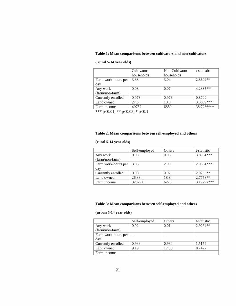
In Table 1 we compare the means of some important variables between
cultivating and non-cultivating households for rural 5-14 year olds. Table 1
shows that on an average a child aged 5-14 years from cultivating households
tend to have significantly higher likelihood of being employed, and also tend
to have higher hours of participation in family farm.
In Tables 2 and 3 we compare the means of hours worked by children aged
5-14 and other variables between self-employed households and other house-
holds for the rural and urban sector respectively. We consider self-employed
houesholds, Self-employed households are those engaged in cultivation, allied
agriculture, petty trade, business and artisanship. Others refer to various
types of employees including agricultural/non-agricultural labourers, salaried
persons, professionals, those on pensions and others. In the rural sector as
with cultivating households, 5-14 year old children from self-employed fam-
ilies are more likely to be working in our sample. In the urban sector also
16

the self-employed households have a higher number of hours worked (which
is statistically significant), though the mean itself is much smaller than the
rural sector means.
Table 4 presents the descriptive statistics of the children, along with their
socio-economic characeristics, such as castes and religion and their parents’
education.
Insert Tables 1-4 here.
4.1 Econometric modelling
Our main interest is to examine what determines the probability of a child
(aged 5-14 years) working. As indicated earlier, we focus on the rural sector.
Let Y1 be a binary variable that takes a value 1 if the child works and 0
otherwise.
Our central hypothesis is to examine the effect of parental self-employment
(measured by a binary variable SE) on Y1. Note however that a self-employed
household may or may not hire labourers (measured by a second binary vari-
able HL) from the market. We also include an interaction between SE and
HL to account for the differential effect of self-employed households on the
probability of Y1 when non-family labourers are hired from the market. Thus
for the i-th child aged 5-14 years from the j-th household residing in the s-th
state, the latent variable denoting propensity to work in the rural sector is
given by
Y ∗1ijs = γESEj + γHHLj + γEHSEj ∗HLj + γ′xX1ij + φs + u1ij (12)
where Y ∗1ij is not observable. We only observe Y1ij where Y1ij = 1 if Y ∗1ij > 0;
Y1ij = 0 otherwise. φs refers to any unobserved state fixed effects and u1
is an iid error term assumed to be distributed with zero mean and constant
variance. X1 refers to all other individual, household or community specific
factors that may affect Y1. Thus after controlling for all other factors, we
focus on the estimates γE, γH , and γEH to test the central hypotheses.
However, the propensity to work for a child aged 5-14 year old cannot be
dissociated from the child’s decision to attend school. So the estimates γE,
17

γH , and γEH are likely to be biased if we ignore the child’s decision to go to
school as well. Let Y2 denote the child’s propensity to attend a school such
that
Y ∗2ijs = β′X2ijs + θs + u2ij. (13)
We only observe Y2ij where Y2ij = 1 if Y ∗2ij > 0; Y2ij = 0 otherwise. Here X2
is a set of individual/child or community specific explanatory variables and
θs is the state fixed effects.
When we individually determine equations (12) and (13), we assume that
the error terms u1 and u2 in (12) and (13) are uncorrelated. Given that we
argue that a child’s participation in school and work are inter-related, we
cannot assume that the two errors are uncorrelated. So we use a bivariate
probit model which allows for the possibility that the two errors in these
two equations are correlated: suppose ρ denotes the correlation between
the two errors. Thus a bivariate probit model will not only determine the
coefficient estimates for the two sets of explanatory variables in (12) and
(13), but will also produce an estimate of ρ. The statistical significance of
the estimated ρ provides a test for the goodness of fit of the bivariate (as
opposed to individual) probit equations for (12) and (13). Note that the
consistent estimates of a bivariate probit model requires that we have some
identifying variables in equations (12) and (13). While we include SE, HL
and also SE∗HL in equation (12), these variables are excluded from equation
(13).
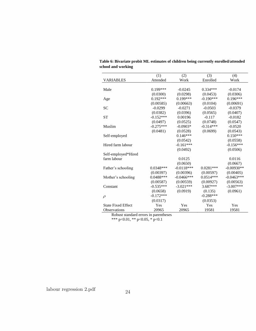
Table 5 shows the univariate probit estimates of equations (12) and (13)
while Table 6 shows the corresponding bivariate probit joint estimates of
propensity to participate in work and school. Columns (1) and (2) of Table
6 show the joint estimates of current enrolment and work participation while
columns (3) and (4) show those for school attendance and work participation.
The significance of ρ in each case justifies the use of bivariate probit model
and hence we couch our discussion in terms of the bivariate probit model.
While estimated coefficient of self-employment SE is positive and significant,
that of HL is negative in the bivariate probit model. However, the interaction
between SE and HL turns out to be negative, though remains insignificant.
In other words, ceteris paribus, children from self-employed households are
more likely to participate in work while those from households hiring outside
labour are less likely to do so. Given that the interaction term is negative
18

(though insignificant), the positive effect of self-employment on incidence of
child labour is muted for the self-employed households who are hiring labour
from the market.
Insert Tables 5 and 6 here.
5 Conclusion
In this paper we demonstrate that in the child labour model of Basu and Van
(1998) the socially inefficient equilibrium which involves the employment of
child labour can be eliminated if some households are empowered with self-
employment opportunities. In equilibrium, the self-employed parents will
split their time between self-employment and a well-paying labour market.
We then also show that if the self-employed parents exclusively work for
themselves and in addition hire their own children as a substitute for outside
labour, they will generate a reverse pattern of child labour. The child will
work when the outside wage is high and stay at school when the outside wage
is low, quite in contrast to the wage workers’ children. Either situation can
emerge in equilibrium depending on the proportion of households engaged in
self-employment. Thus, we provide an explanation of greater child labour in
the self-employment sector, which has been evidenced by data.
The key intuition of this study is that modestly remunerative self-employment
works well at low wages as it implements an income floor. But at higher
wages, it is unattractive and the parent needs to switch back to wage em-
ployment. If he cannot or does not do so, self-employment can be a curse.
From the policy point of view it may be said that measures to promote
self-employment will in general have a good effect. However, it is important
to ensure that self-employment projects are sufficiently remunerative. They
must generate sufficiently large incomes to generate adequate income effects.
Given paucity of public funds, policy makers may have to choose between
how much assistance to be provided per individual as opposed to how many
individuals to be assisted. The overall impact is more beneficial if fewer
people are given a sizable fund each to switch to self-employment, rather
than giving a smaller fund each to a large number of individuals.
19

References
1. Baland, J-M. and Robinson, J. A. (2000) Is child labor inefficient?
Journal of Political Economy 108: 663-79.
2. Basu, K. (2000) The intriguing relation between adult minimum wage
and child labour. Economic Journal 110 (462): C50-61.
3. Basu, K. and Van, P. H. (1998) The Economics of child labor. American
Economic Review 88: 412-27.
4. Basu, K., Das, S. and Dutta, B. (2009) Child labor and household
wealth: Theory and empirical evidence of an inverted-U. Journal of De-
velopment Economics forthcoming, doi:10.1016/j.jdeveco.2009.91.006.
5. Bhalotra, S. and Heady, C. (2003) Child farm labor: The wealth para-
dox. World Bank Economic Review 17: 197-227.
6. Gupta, M. R. (2000) Wage determination of a child worker: A theoret-
ical analysis. Review of Development Economics 4: 219-28.
7. Jafarey, S. and Lahiri, S. (2002) Will trade sanctions reduce child
labour? The role of credit markets. Journal of Development Economics
68: 137-56
8. Parikh, A. and Sadoulet, E. (2005) The effects of parents’ occupation
on child labor and school attendance in Brazil.
http://are.berkeley.edu/ sadoulet/papers/Childlabour.pdf
9. Ranjan, P. (2001) Credit constraints and the phenomenon of child la-
bor. Journal of Development Economics 64: 81-102.
20
labour descriptives 1.pdf
Table 1: Mean comparisons between cultivators and non-cultivators
( rural 5-14 year olds)
Cultivator
households
Non-Cultivator
households
t-statistic
Farm work-hours per
day
3.38 3.04 2.8694**
Any work
(farm/non-farm)
0.08 0.07 4.2335***
Currently enrolled 0.978 0.976 0.8799
Land owned 27.5 18.8 3.3639***
Farm income 40752 6859 38.7236***
*** p<0.01, ** p<0.05, * p<0.1
Table 2: Mean comparisons between self-employed and others
(rural 5-14 year olds)
Self-employed Others t-statistic
Any work
(farm/non-farm)
0.08 0.06 3.8904***
Farm work-hours per
day
3.36 2.99 2.9864***
Currently enrolled 0.98 0.97 2.0255**
Land owned 26.33 18.8 2.7778**
Farm income 32879.6 6273 30.9297***
Table 3: Mean comparisons between self-employed and others
(urban 5-14 year olds)
Self-employed Others t-statistic
Any work
(farm/non-farm)
0.02 0.01 2.9264**
Farm work-hours per
day
- - -
Currently enrolled 0.988 0.984 1.5154
Land owned 9.19 17.38 0.7427
Farm income - - -
21

labour descriptives 2.pdf
Table 4: Means of children’s characteristics (Rural)
Variable Obs. Mean
Std.
Dev.
If currently enrolled 21944 0.977397 0.148638
If doing any work 23511 0.071286 0.257307
Male 23511 0.520097 0.499607
Age (years) 23511 9.699077 2.784947
Scheduled Caste 23511 0.222619 0.416014
Scheduled Tribe 23511 0.093403 0.291003
Muslim 23511 0.121645 0.326883
Weight (kg) 9184 22.29277 6.986225
Self-employed hh 23511 0.509123 0.499927
If hired any farm-labour 23511 0.743312 0.436815
If selfemp and hired
outside farm labour 23511 0.372634 0.483516
Father's schooling (years) 21290 5.394974 4.567116
Mother's schooling
(years) 22682 2.702584 3.791032
Source: IHDS 2005-2006 sample, authors’ calculation
22

labour regression1.pdf
Table 5: Univariate Probit estimates of school attended, currently
enrolled and any work among enrolled, rural 15-14 year olds
(2) (3) (9)
VARIABLES Attended
school
Currently
enrolled
Doing any
work
Male 0.225*** 0.135 -0.0305*
(0.0542) (0.112) (0.0178)
Age 0.415*** 0.0318 0.205***
(0.0219) (0.0434) (0.00475)
SC 0.0314 0.0491 -0.0280
(0.0708) (0.139) (0.0406)
ST -0.148 -0.0697 0.00324
(0.0976) (0.195) (0.0575)
Muslim -0.189** -0.0727 -0.0852**
(0.0961) (0.149) (0.0360)
Self-employed 0.150**
(0.0592)
Hired farm labour -0.157***
(0.0374)
Self-employed*Hired
farm labour
0.00539
(0.0525)
Father’s schooling (yrs) 0.0362*** 0.0185 -0.0130***
(0.00734) (0.0137) (0.00372)
Mother’s schooling (yrs) 0.0569*** 0.00838 -0.0466***
(0.0101) (0.0198) (0.00211)
Weight (kg) 0.0196** -0.0118**
(0.00783) (0.00546)
Constant -2.483*** 2.338*** -3.072***
(0.167) (0.425) (0.0522)
State Fixed Effect Yes Yes Yes
Observations 8230 7164 20528
Robust standard errors in parentheses
** p<0.01, ** p<0.05, * p<0.1
23
labour regression 2.pdf
Table 6: Bivariate probit ML estimates of children being currently enrolled/attended
school and working
(1) (2) (3) (4)
VARIABLES Attended Work Enrolled Work
Male 0.199*** -0.0245 0.334*** -0.0174
(0.0300) (0.0298) (0.0453) (0.0306)
Age 0.192*** 0.199*** -0.190*** 0.196***
(0.00585) (0.00663) (0.0104) (0.00691)
SC -0.0299 -0.0271 -0.0503 -0.0379
(0.0382) (0.0396) (0.0565) (0.0407)
ST -0.152*** 0.00196 -0.117 -0.0182
(0.0497) (0.0525) (0.0748) (0.0547)
Muslim -0.275*** -0.0903* -0.314*** -0.0520
(0.0481) (0.0528) (0.0699) (0.0543)
Self-employed 0.146*** 0.150***
(0.0542) (0.0558)
Hired farm labour -0.161*** -0.156***
(0.0492) (0.0506)
Self-employed*Hired
farm labour
0.0125
0.0116
(0.0650) (0.0667)
Father’s schooling 0.0348*** -0.0118*** 0.0281*** -0.00930**
(0.00397) (0.00396) (0.00597) (0.00405)
Mother’s schooling 0.0488*** -0.0466*** 0.0514*** -0.0463***
(0.00587) (0.00559) (0.00927) (0.00563)
Constant -0.535*** -3.021*** 3.687*** -3.007***
(0.0658) (0.0919) (0.135) (0.0961)
-0.172*** -0.288***
(0.0317) (0.0353)
State Fixed Effect Yes Yes Yes Yes
Observations 20965 20965 19581 19581
Robust standard errors in parentheses
*** p<0.01, ** p<0.05, * p<0.1
24