Structured eigenvalue condition numbers and

linearizations for matrix polynomials∗

Bibhas Adhikari† Rafikul Alam‡ Daniel Kressner§.

Abstract. This work is concerned with eigenvalue problems for structured matrix polynomials,

including complex symmetric, Hermitian, even, odd, palindromic, and anti-palindromic matrix poly-

nomials. Most numerical approaches to solving such eigenvalue problems proceed by linearizing the

matrix polynomial into a matrix pencil of larger size. Recently, linearizations have been classified

for which the pencil reflects the structure of the original polynomial. A question of practical impor-

tance is whether this process of linearization significantly increases the eigenvalue sensitivity with

respect to structured perturbations. For all structures under consideration, we show that this cannot

happen if the matrix polynomial is well scaled: There is always a structured linearization for which

the structured eigenvalue condition number does not differ much. This implies, for example, that

a structure-preserving algorithm applied to the linearization fully benefits from a potentially low

structured eigenvalue condition number of the original matrix polynomial.

Keywords. Eigenvalue problem, matrix polynomial, linearization, structured condition num-ber.

AMS subject classification(2000): 65F15, 15A57, 15A18, 65F35.

1 Introduction

Consider an n× n matrix polynomial

P(λ) = A0 + λA1 + λ2A2 + · · ·+ λmAm, (1)

with A0, . . . , Am ∈ Cn×n. An eigenvalue λ ∈ C of P, defined by the relation det(P(λ)) = 0,is called simple if λ is a simple root of the polynomial det(P(λ)).

This paper is concerned with the sensitivity of a simple eigenvalue λ under perturbationsof the coefficients Ai. The condition number of λ is a first-order measure for the worst-caseeffect of perturbations on λ. Tisseur [35] has provided an explicit expression for this conditionnumber. Subsequently, this expression was extended to polynomials in homogeneous form byDedieu and Tisseur [10], see also [1, 5, 9], and to semi-simple eigenvalues in [24]. In themore general context of nonlinear eigenvalue problems, the sensitivity of eigenvalues andeigenvectors has been investigated in, e.g., [3, 26, 27, 28].

Loosely speaking, an eigenvalue problem (1) is called structured if there is some distinctivestructure among the coefficients A0, . . . , Am. For example, much of the recent research onstructured polynomial eigenvalue problems was motivated by the second-order T -palindromiceigenvalue problem [20, 29]

A0 + λA1 + λ2AT0 ,

where A1 is complex symmetric: AT1 = A1. In this paper, we consider the structures listedin Table 1. To illustrate the notation of this table, consider a T -palindromic polynomial∗Revision dated January 18, 2011.†Department of Mathematics, Indian Institute of Technology Guwahati, India, E-mail: bibhas@iitg.ernet.in‡Department of Mathematics, Indian Institute of Technology Guwahati, India, E-mail: rafik@iitg.ernet.in,

rafikul@yahoo.com, Fax: +91-361-2690762/2582649.§Seminar for Applied Mathematics, ETH Zurich, Switzerland. E-mail: kressner@sam.math.ethz.ch

Structured Polynomial P(λ) =∑mi=0 λ

iAi

Structure Condition m = 2

symmetric PT (λ) = P(λ) P(λ) = λ2A0 + λA1 +A2,

AT0 = A0, AT1 = A1, A

T2 = A2

Hermitian PH(λ) = P(λ) P(λ) = λ2A0 + λA1 +A2,

AH0 = A0, AH1 = A1, A

H2 = A2

?-even P?(λ) = P(−λ) P(λ) = λ2A+ λB + C,

A? = A,B? = −B,C? = C

?-odd P?(λ) = −P(−λ) P(λ) = λ2A+ λB + C,

A? = −A,B? = B,C? = −C?-palindromic P?(λ) = λmP(1/λ) P(λ) = λ2A+ λB +A?, B? = B

?-anti-palindromic P?(λ) = λmP(−1/λ) P(λ) = λ2A+ λB −A?, B? = −B

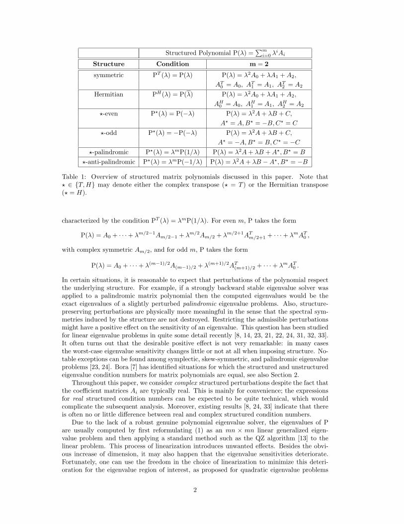
Table 1: Overview of structured matrix polynomials discussed in this paper. Note that? ∈ {T,H} may denote either the complex transpose (? = T ) or the Hermitian transpose(? = H).

characterized by the condition PT (λ) = λmP(1/λ). For even m, P takes the form

P(λ) = A0 + · · ·+ λm/2−1Am/2−1 + λm/2Am/2 + λm/2+1ATm/2+1 + · · ·+ λmAT0 ,

with complex symmetric Am/2, and for odd m, P takes the form

P(λ) = A0 + · · ·+ λ(m−1)/2A(m−1)/2 + λ(m+1)/2AT(m+1)/2 + · · ·+ λmAT0 .

In certain situations, it is reasonable to expect that perturbations of the polynomial respectthe underlying structure. For example, if a strongly backward stable eigenvalue solver wasapplied to a palindromic matrix polynomial then the computed eigenvalues would be theexact eigenvalues of a slightly perturbed palindromic eigenvalue problems. Also, structure-preserving perturbations are physically more meaningful in the sense that the spectral sym-metries induced by the structure are not destroyed. Restricting the admissible perturbationsmight have a positive effect on the sensitivity of an eigenvalue. This question has been studiedfor linear eigenvalue problems in quite some detail recently [8, 14, 23, 21, 22, 24, 31, 32, 33].It often turns out that the desirable positive effect is not very remarkable: in many casesthe worst-case eigenvalue sensitivity changes little or not at all when imposing structure. No-table exceptions can be found among symplectic, skew-symmetric, and palindromic eigenvalueproblems [23, 24]. Bora [7] has identified situations for which the structured and unstructuredeigenvalue condition numbers for matrix polynomials are equal, see also Section 2.

Throughout this paper, we consider complex structured perturbations despite the fact thatthe coefficient matrices Ai are typically real. This is mainly for convenience; the expressionsfor real structured condition numbers can be expected to be quite technical, which wouldcomplicate the subsequent analysis. Moreover, existing results [8, 24, 33] indicate that thereis often no or little difference between real and complex structured condition numbers.

Due to the lack of a robust genuine polynomial eigenvalue solver, the eigenvalues of Pare usually computed by first reformulating (1) as an mn × mn linear generalized eigen-value problem and then applying a standard method such as the QZ algorithm [13] to thelinear problem. This process of linearization introduces unwanted effects. Besides the obvi-ous increase of dimension, it may also happen that the eigenvalue sensitivities deteriorate.Fortunately, one can use the freedom in the choice of linearization to minimize this deteri-oration for the eigenvalue region of interest, as proposed for quadratic eigenvalue problems

2

in [11, 19, 35]. For the general polynomial eigenvalue problem (1), Higham et al. [18, 16] haveidentified linearizations with minimal eigenvalue condition number/backward error among theset of linearizations described in [30]. For structured polynomial eigenvalue problems, ratherthan using any linearization it is of course advisable to use one which has a similar structure.For example, it was shown in [29] that a palindromic matrix polynomial can usually be lin-earized into a palindromic or anti-palindromic matrix pencil, offering the possibility to applystructure-preserving algorithms to the linearization. It is natural to ask whether there is alsoa structured linearization that has no adverse effect on the structured condition number. Fora small subset of structures from Table 1, this question has already been discussed in [18]. Inthe second part of this paper, we extend the discussion to all structures from Table 1.

The rest of this paper is organized as follows. In Section 2, we first review the derivationof the unstructured eigenvalue condition number for a matrix polynomial and then provideexplicit expressions for structured eigenvalue conditions numbers. In Section 4, we applythese results to find good choices from the set of structured linearizations described in [29].

2 Structured condition numbers for matrix polynomials

Before discussing the effect of structure on the sensitivity of an eigenvalue, we briefly reviewexisting results on eigenvalue condition numbers for matrix polynomials. Assume that λ is asimple finite eigenvalue of the matrix polynomial P defined in (1) with normalized right andleft eigenvectors x and y:

P(λ)x = 0, yHP(λ) = 0, ‖x‖2 = ‖y‖2 = 1. (2)

The perturbation

(P +4P)(λ) = (A0 + E0) + λ(A1 + E1) + · · ·+ λm(Am + Em)

moves λ to an eigenvalue λ of P +4P. A useful tool to study the effect of 4P is the firstorder perturbation expansion

λ = λ− 1yHP′(λ)x

yH4P(λ)x+O(‖4P‖2), (3)

which can be derived, e.g., by applying the implicit function theorem to (2), see [10, 35]. Notethat yHP′(λ)x 6= 0 because λ is simple [3].

To measure the sensitivity of λ we first need to specify a way to measure 4P. Given amatrix norm ‖·‖M on Cn×n, a monotone vector norm ‖·‖V on Cm+1 and non-negative weightsω0, . . . , ωm, we define

‖4P‖ :=∥∥∥∥[ 1ω0‖E0‖M,

1ω1‖E1‖M, . . . ,

1ωm‖Em‖M

]∥∥∥∥V

. (4)

A relatively small weight ωi means that ‖Ei‖M will be small compared to ‖4P‖. In theextreme case ωi = 0, we define ‖Ei‖M/ωi = 0 for ‖Ei‖M = 0 and ‖Ei‖M/ωi = ∞ otherwise.If all ωi are positive then (4) defines a norm on Cn×n × · · · × Cn×n, see [2, 1] for more onnorms of matrix polynomials.

We are now ready to introduce a condition number for the eigenvalue λ of P with respectto the choice of ‖4P‖ in (4):

κP(λ) := limε→0

sup{ |λ− λ|

ε: ‖4P‖ ≤ ε

}, (5)

where λ is the eigenvalue of P +4P closest to λ. An explicit expression for κP(λ) can befound in [35, Thm. 5] for the case ‖ · ‖V ≡ ‖ · ‖∞ and ‖ · ‖M ≡ ‖ · ‖2. In contrast, the approach

3

used in [10] requires an accessible geometry on the perturbation space and thus facilitates thenorms ‖ · ‖V ≡ ‖ · ‖2 and ‖ · ‖M ≡ ‖ · ‖F . Lemma 2.1 below is more general and includes bothsettings. For stating our result, we recall that the dual to the vector norm ‖ · ‖V is defined as

‖w‖D := sup‖z‖V≤1

|wT z|,

see, e.g., [15].

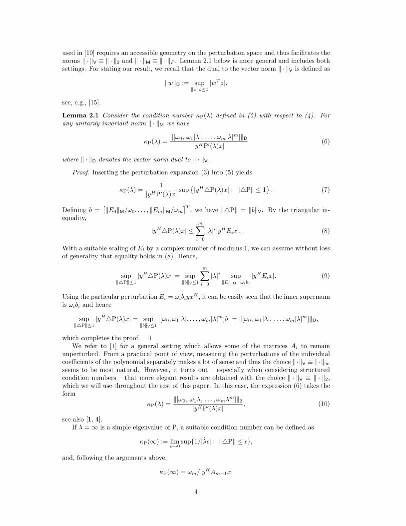
Lemma 2.1 Consider the condition number κP(λ) defined in (5) with respect to (4). Forany unitarily invariant norm ‖ · ‖M we have

κP(λ) =‖[ω0, ω1|λ|, . . . , ωm|λ|m]‖D

|yHP′(λ)x|(6)

where ‖ · ‖D denotes the vector norm dual to ‖ · ‖V.

Proof. Inserting the perturbation expansion (3) into (5) yields

κP(λ) =1

|yHP′(λ)x|sup

{|yH4P(λ)x| : ‖4P‖ ≤ 1

}. (7)

Defining b =[‖E0‖M/ω0, . . . , ‖Em‖M/ωm

]T , we have ‖4P‖ = ‖b‖V. By the triangular in-equality,

|yH4P(λ)x| ≤m∑i=0

|λ|i|yHEix|. (8)

With a suitable scaling of Ei by a complex number of modulus 1, we can assume without lossof generality that equality holds in (8). Hence,

sup‖4P‖≤1

|yH4P(λ)x| = sup‖b‖V≤1

m∑i=0

|λ|i sup‖Ei‖M=ωibi

|yHEix|. (9)

Using the particular perturbation Ei = ωibiyxH , it can be easily seen that the inner supremum

is ωibi and hence

sup‖4P‖≤1

|yH4P(λ)x| = sup‖b‖V≤1

∣∣[ω0, ω1|λ|, . . . , ωm|λ|m]b∣∣ = ‖[ω0, ω1|λ|, . . . , ωm|λ|m]‖D,

which completes the proof.We refer to [1] for a general setting which allows some of the matrices Ai to remain

unperturbed. From a practical point of view, measuring the perturbations of the individualcoefficients of the polynomial separately makes a lot of sense and thus the choice ‖·‖V ≡ ‖·‖∞seems to be most natural. However, it turns out – especially when considering structuredcondition numbers – that more elegant results are obtained with the choice ‖ · ‖V ≡ ‖ · ‖2,which we will use throughout the rest of this paper. In this case, the expression (6) takes theform

κP(λ) =‖[ω0, ω1λ, . . . , ωmλ

m]‖2|yHP′(λ)x|

, (10)

see also [1, 4].If λ =∞ is a simple eigenvalue of P, a suitable condition number can be defined as

κP(∞) := limε→0

sup{1/|λε| : ‖4P‖ ≤ ε},

and, following the arguments above,

κP(∞) = ωm/|yHAm−1x|

4

for any (Holder) p-norm ‖ · ‖V. Note that this discrimination between finite and infiniteeigenvalues disappears when homogenizing P as in [10] or measuring the distance betweenperturbed eigenvalues with the chordal metric as in [34]. In order to keep the presentationsimple, we have decided not to use these concepts.

The rest of this section is concerned with quantifying the effect on the condition num-ber when the perturbation 4P is restricted to a subset S of the space of all n × n matrixpolynomials of degree at most m.

Definition 2.2 Let λ be a simple finite eigenvalue of a matrix polynomial P with normalizedright and left eigenvectors x and y. Then the structured condition number of λ with respectto S is defined as

κSP(λ) := lim

ε→0sup

{|λ− λ|ε

: 4P ∈ S, ‖4P‖ ≤ ε

}(11)

For a simple infinite eigenvalue λ, κSP(∞) := lim

ε→0sup{1/|λε| : 4P ∈ S, ‖4P‖ ≤ ε}.

If S is a star-shaped set [12] with respect to 0, the expansion (3) can be used to show

κSP(λ) =

1|yHP′(λ)x|

sup{|yH4P(λ)x| : 4P ∈ S, ‖4P‖ ≤ 1

}(12)

andκS

P(∞) =1

|yHAm−1x|sup

{|yHEmx| : 4P ∈ S, ‖Em‖M ≤ ωm

}. (13)

The formulation (12) is the starting point to derive explicit expressions for κSP under

particular choices of S. To proceed, one can employ results by Karow [21] on the geometryof the set {yHEx : E ∈ E, ‖E‖M ≤ 1} with respect to some matrix structures E ⊆ Cn×ninduced by the polynomial structure S. Such an approach was proposed by Bora [7], whoalso derived explicit expressions and bounds on κS

P for the structures considered in this paper.Our expressions are of a similar nature and we therefore defer the derivations to Appendix A.The major difference is that we use ‖ · ‖V ≡ ‖ · ‖2 while [7] uses ‖ · ‖V ≡ ‖ · ‖∞ for combiningthe norm of perturbations in the polynomial coefficients, see (4). We deliberately choose the2-norm setting as this allows simpler explicit expressions for structured eigenvalue conditionnumbers. This in turn enables easy comparison of structured eigenvalue condition numbersof structured polynomials with those of the structured linearizations discussed in Section 4.

2.1 Complex symmetric matrix polynomials

No or only an insignificant decrease of the condition number can be expected when imposingcomplex symmetries on the perturbations of a matrix polynomial.

Lemma 2.3 Let S denote the set of complex symmetric matrix polynomials. Then for a finiteor infinite, simple eigenvalue λ of a matrix polynomial P,

1. κSP(λ) = κP(λ) for ‖ · ‖M ≡ ‖ · ‖2, and

2. κSP(λ) =

√1+|yT x|2√

2κP(λ) for ‖ · ‖M ≡ ‖ · ‖F .

2.2 T -even and T -odd matrix polynomials

To describe the structured condition numbers for T -even and T -odd polynomials in a conve-nient manner, we introduce the vector

Λω =[ωmλ

m, ωm−1λm−1, . . . , ω1λ, ω0

]T (14)

5

along with the even coefficient projector

Πe : Λω 7→ Πe(Λω) :=

{ [ωmλ

m, 0, ωm−2λm−2, 0, . . . , ω2λ

2, 0, ω0

]T, if m is even,[

0, ωm−1λm−1, 0, ωm−3λ

m−3, . . . , 0, ω0

]T, if m is odd.

(15)

The odd coefficient projection is defined analogously and satisfies Πo(Λω) = Λω −Πe(Λω).

Lemma 2.4 Let S denote the set of all T -even matrix polynomials. Then for a finite, simpleeigenvalue λ of a matrix polynomial P,

1. κSP(λ) =

√1− |yTx|2 ‖Πo(Λω)‖22

‖Λω‖22κP(λ) for ‖ · ‖M ≡ ‖ · ‖2, and

2. κSP(λ) = 1√

2

√1− |yTx|2 ‖Πo(Λω)‖22−‖Πe(Λω)‖22

‖Λω‖22κP(λ) for ‖ · ‖M ≡ ‖ · ‖F .

For an infinite, simple eigenvalue,

3. κSP(∞) =

{κP(∞), if m is even,√

1− |yTx|2 κP (∞), if m is odd,for ‖ · ‖M ≡ ‖ · ‖2, and

4. κSP(∞) =

{1√2

√1 + |yTx|2κP(∞), if m is even,

1√2

√1− |yTx|2κP(∞), if m is odd,

for ‖ · ‖M ≡ ‖ · ‖F .

Remark 2.5 Note that the statement of Lemma 2.4 does not assume that P itself is T -even.If we impose this condition then, for odd m, P has a simple infinite eigenvalue only if alsothe size of P is odd, see, e.g., [24]. In this case, the skew-symmetry of Am forces the infiniteeigenvalue to be preserved under arbitrary structure-preserving perturbations. This is reflectedby κS

P(∞) = 0.

Lemma 2.4 reveals that the structured condition number can only be significantly lowerthan the unstructured one if |yTx| and the ratio

‖Πo(Λω)‖22‖Λω‖22

=

∑i odd

ω2i |λ|2i∑

i=0,...,m

ω2i |λ|2i

= 1−

∑i even

ω2i |λ|2i∑

i=0,...,m

ω2i |λ|2i

are close to one. The most likely situation for the latter ratio to become close to one is whenm is odd, ωm does not vanish, and |λ| is large.

Example 2.6 ([33]) Let

P(λ) = I + λ0 + λ2I + λ3

0 1− φ 0−1 + φ 0 i

0 −i 0

with 0 < φ < 1. This matrix polynomial has one eigenvalue λ∞ = ∞ because of the highestcoefficient, which is – as any odd-sized skew-symmetric matrix – singular. The following tableadditionally displays the eigenvalue λmax of largest magnitude, the eigenvalue λmin of smallestmagnitude, as well as their unstructured and structured condition numbers for the set S ofT -even matrix polynomials. We have chosen ωi = ‖Ai‖2 and ‖ · ‖M ≡ ‖ · ‖2.

φ 100 10−3 10−9

κ(λ∞) 1 1.4× 103 1.4× 109

κSP(λ∞) 0 0 0|λmax| 1.47 22.4 2.2× 104

κP(λmax) 1.12 3.5× 105 3.5× 1017

κSP(λmax) 1.12 2.5× 104 2.5× 1013

|λmin| 0.83 0.99 1.00κP(λmin) 0.45 5.0× 102 5.0× 108

κSP(λmin) 0.45 3.5× 102 3.5× 108

6

The entries 0 = κSP(λ∞) � κP(λ∞) reflect the fact that the infinite eigenvalue stays intact

under structure-preserving but not under general perturbations. For the largest eigenvalues,we observe a significant difference between the structured and unstructured condition numbersas φ→ 0. In contrast, this difference becomes negligible for the smallest eigenvalues.

Remark 2.7 For even m, the structured eigenvalue condition number of a T -even polynomialis usually close to the unstructured one. For example if all weights are equal, ‖Πo(Λ)‖22 ≤‖Λ‖22/2 implying κS

P(λ) ≥ κP(λ)/√

2 for ‖ · ‖M ≡ ‖ · ‖2.

For T -odd polynomials, we obtain the following analogue of Lemma 2.4 by simply ex-changing the roles of odd and even in the proof.

Lemma 2.8 Let S denote the set of all T -odd matrix polynomials. Then for a finite, simpleeigenvalue λ of a matrix polynomial P,

1. κSP(λ) =

√1− |yTx|2 ‖Πe(Λω)‖22

‖Λω‖22κP(λ) for ‖ · ‖M ≡ ‖ · ‖2, and

2. κSP(λ) = 1√

2

√1− |yTx|2 ‖Πe(Λω)‖22−‖Πo(Λω)‖22

‖Λω‖22κP(λ) for ‖ · ‖M ≡ ‖ · ‖F .

For an infinite, simple eigenvalue,

3. κSP(∞) =

{κP(∞), if m is odd,0, if m is even, for ‖ · ‖M ≡ ‖ · ‖2, and

4. κSP(∞) =

{1√2

√1 + |yTx|2κP(∞), if m is odd,

0, if m is even,for ‖ · ‖M ≡ ‖ · ‖F .

Similar to the discussion above, the only situation for which κSP(λ) can be expected to become

significantly smaller than κP(λ) when |yTx| ≈ 1 and λ ≈ 0.

2.3 T -palindromic and T -anti-palindromic matrix polynomials

For a T -palindromic polynomial it is sensible to require that the weights in the choice of‖4P‖, see (4), satisfy ωi = ωm−i. This condition is tacitly assumed throughout the entiresection. The Cayley transform for polynomials introduced in [29, Sec. 2.2] defines a mappingbetween palindromic/anti-palindromic and odd/even polynomials. As already demonstratedin [24] for the case m = 1, this idea can be used to transfer the results from the previoussection to the (anti-)palindromic case. For the mapping to preserve the underlying norm wehave to restrict ourselves to the case ‖ · ‖M ≡ ‖ · ‖F . The coefficient projections appropriatefor palindromic polynomials are given by Π± : Λω 7→ Π±(Λω) with

Π±(Λω) :=

{[ω0

λm±1√2, . . . , ωm/2−1

λm/2+1±λm/2−1√

2, ωm/2

λm/2±λm/22

]T if m is even,[ω0

λm±1√2, . . . , ω(m−1)/2

λ(m+1)/2±λ(m−1)/2√

2

]T, if m is odd.

(16)

Note that ‖Π+(Λω)‖22 + ‖Π−(Λω)‖22 = ‖Λω‖22.

Lemma 2.9 Let S denote the set of all T -palindromic matrix polynomials. Then for a finite,simple eigenvalue λ of a matrix polynomial P, with ‖ · ‖M ≡ ‖ · ‖F ,

κSP(λ) =

1√2

√1 + |yTx|2 ‖Π+(Λω)‖22 − ‖Π−(Λω)‖22

‖Λω‖22κP(λ).

For an infinite, simple eigenvalue, κSP(∞) = κP(∞).

7

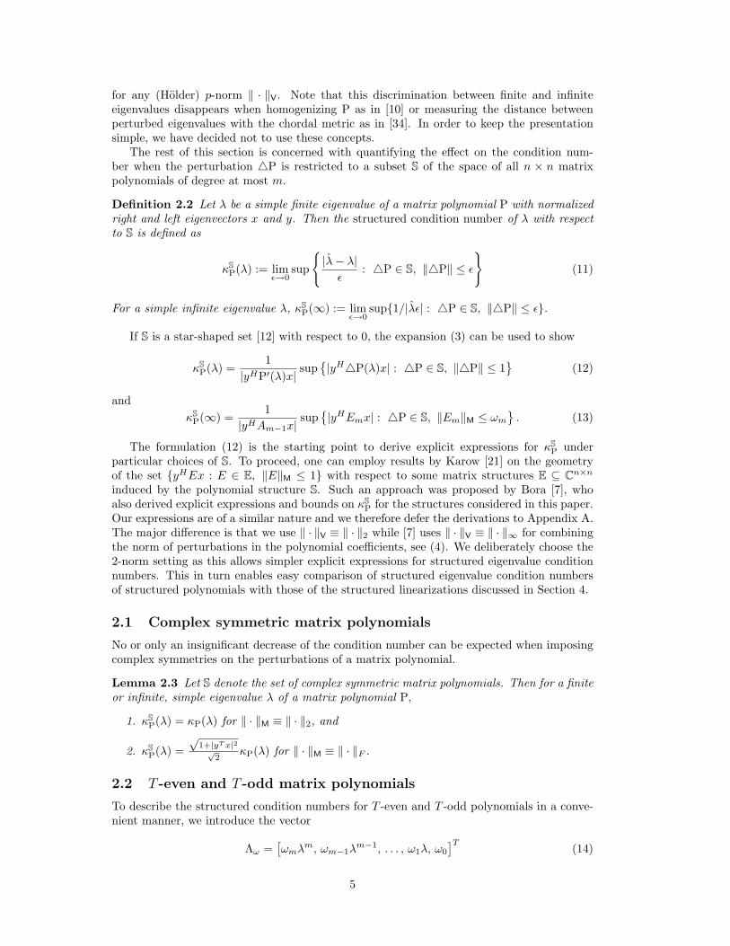
From the result of Lemma 2.9 it follows that a large difference between the structuredand unstructured condition numbers for T -palindromic matrix polynomials may occur when|yTx| is close to one, and ‖Π+(Λω)‖2 is close to zero. Assuming that all weights are positive,the latter condition implies that m is odd and and λ ≈ −1. An instance of such a case isgiven by a variation of Example 2.6.

Example 2.10 Consider the T -palindromic matrix polynomial

P(λ) =

1 1− φ 0−1 + φ 1 i

0 −i 1

+ λI + λ2I − λ3

1 1− φ 0−1 + φ 1 i

0 −i 1

with 0 < φ < 1. An odd-sized T -palindromic matrix polynomial, P has the eigenvalue λ−1 =−1. The following table additionally displays one eigenvalue λclose closest to −1, an eigenvalueλmin of smallest magnitude, as well as their unstructured and structured condition numbers forthe set S of T -palindromic matrix polynomials. We have chosen ωi = ‖Ai‖F and ‖·‖M ≡ ‖·‖F .

φ 10−1 10−4 10−8

κ(λ−1) 20.9 2.2× 104 2.2× 108

κSP(λ−1) 0 0 0

|1 + λclose| 0.39 1.4× 10−2 1.4× 10−4

κP(λclose) 11.1 1.1× 104 1.1× 108

κSP(λclose) 6.38 2.5× 102 2.6× 104

|1 + λmin| 1.25 1.41 1.41κP(λmin) 7.92 7.9× 103 7.9× 107

κSP(λmin) 5.75 5.6× 103 5.6× 107

The entries 0 = κSP(λ−1) � κP(λ−1) reflect the fact that the eigenvalue −1 remains intact

under structure-preserving but not under general perturbations. Also, eigenvalues close to −1benefit from a significantly lower structured condition numbers as φ→ 0. In contrast, only apractically irrelevant benefit is revealed for the eigenvalue λmin not close to −1.

Results analogous to Lemma 2.9 hold for T -anti-palindromic matrix polynomials.

Lemma 2.11 Let S denote the set of all T -anti-palindromic matrix polynomials. Then for afinite, simple eigenvalue λ of a matrix polynomial P, with ‖ · ‖M ≡ ‖ · ‖F ,

κSP(λ) =

1√2

√1− |yTx|2 ‖Π+(Λω)‖22 − ‖Π−(Λω)‖22

‖Λω‖22κP(λ).

For an infinite, simple eigenvalue, κSP(∞) = κP(∞).

2.4 Hermitian matrix polynomials

For reasons explained in Section A.2, the structured eigenvalue condition numbers for Hermi-tian matrix polynomials do not admit a simple explicit expression. Therefore, the followinglemma rather presents a bound implying that the unstructured and structured eigenvaluecondition numbers are nearly the same.

Lemma 2.12 Let S denote the set of all Hermitian matrix polynomials. Then for a finite orinfinite, simple eigenvalue of a matrix polynomial P,

1.√

1− 12 |yHx|2 κP(λ) ≤ κS

P(λ) ≤ κP(λ) for ‖ · ‖M ≡ ‖ · ‖2, and

2. κP(λ)/√

2 ≤ κSP(λ) ≤ κP(λ) for ‖ · ‖M ≡ ‖ · ‖F .

8

Remark 2.13 Since Hermitian and skew-Hermitian matrices are related by multiplicationwith i, which simply rotates the first-order perturbation set by 90 degrees, a slight modificationof the proof shows that the statement of Lemma 2.12 remains true when S denotes the spaceof H-odd or H-even polynomials. This can in turn be used – as in the proof of Lemma 2.9– to show that also for H-(anti-)palindromic polynomials there is at most an insignificantdifference between the structured and unstructured eigenvalue condition numbers.

3 Condition numbers for linearizations

As already mentioned in the introduction, polynomial eigenvalue problems are often solved bylinearizing the matrix polynomial into a larger matrix pencil. Of the classes of linearizationsproposed in the literature, the vector spaces introduced in [30] are particularly amenable tofurther analysis, while offering a degree of generality that is often sufficient in applications.

Definition 3.1 Let Λm−1 = [λm−1, λm−2 . . . λ, 1]T and let P be a matrix polynomial ofdegree m. Then a matrix pencil L(λ) = λX +Y ∈ Cmn×mn is in DL(P) if there is a so calledansatz vector v ∈ Cm satisfying

L(λ) · (Λm−1 ⊗ I) = v ⊗ P (λ) and (ΛTm−1 ⊗ I) · L(λ) = vT ⊗ P (λ).

It is easy to see that the ansatz vector v is uniquely determined by L ∈ DL(P). In [30,Thm. 6.7] it has been shown that L ∈ DL(P) is a linearization of P if and only if none of theeigenvalues of P is a root of the polynomial

p(µ; v) = v1µm−1 + v2µ

m−2 + · · ·+ vm−1µ+ vm (17)

associated with the ansatz vector v. If P has eigenvalue ∞, this condition should be readas v1 6= 0. Apart from this elegant characterization, probably the most important propertyof DL(P) is that it leads to a simple one-to-one relation between the eigenvectors of P andL ∈ DL(P). To keep the notation compact, we define Λm−1 as in Definition 3.1 for finite λbut let Λm−1 = [1, 0, . . . , 0]T for λ =∞.

Theorem 3.2 ([30]) Let P be a matrix polynomial and L ∈ DL(P) with ansatz vector v.Then x 6= 0 is a right eigenvector of P associated with an eigenvalue λ if and only if Λm−1⊗xis a right eigenvector of L associated with λ. Similarly, y 6= 0 is a left eigenvector of Passociated with an eigenvalue λ if and only if Λm−1 ⊗ y is a left eigenvector of L associatedwith λ.

As a matrix pencil L(λ) = λX+Y is a special case of a matrix polynomial, we can use theresults of Section 2 to study the (structured) eigenvalue condition numbers of L. To simplifythe analysis, we will assume that the weights ω0, . . . , ωm in the definition of ‖4P‖ are all equalto 1 for the rest of this paper. This assumption is only justified if P is not badly scaled, i.e.,the norms of the coefficients of P do not vary significantly. To a certain extent, bad scalingcan be overcome by rescaling the matrix polynomial before linearization, see [6, 11, 16, 18, 19].Moreover, we assume that ‖ · ‖M is an arbitrary but fixed unitarily invariant matrix norm.The same norm is used for measuring perturbations 4L(λ) = 4X+λ4Y to the linearizationL. To summarize

‖4P‖ =√‖E0‖2M + ‖E1‖M + · · ·+ ‖Em‖2M, (18)

‖4L‖ =√‖4X‖2M + ‖4Y ‖2M, (19)

for the rest of this paper. For unstructured eigenvalue condition numbers, Lemma 2.1 togetherwith Theorem 3.2 imply the following formula.

9

Lemma 3.3 Let λ be a finite, simple eigenvalue of a matrix polynomial P with normalizedright and left eigenvectors x and y. Then the eigenvalue condition number κL(λ) for a lin-earization L ∈ DL(P) with ansatz vector v satisfies

κL(λ) =

√1 + |λ|2|p(λ; v)|

· ‖Λm−1‖22|yHP ′(λ)x|

=

√1 + |λ|2 ‖Λm−1‖22|p(λ; v)| ‖Λm‖2

κP(λ).

Proof. A similar formula for the case ‖ · ‖V ≡ ‖ · ‖1 can be found in [18, Section 3]. Theproof for our case ‖ · ‖V ≡ ‖ · ‖2 is almost identical and therefore omitted.

To allow for a simple interpretation of the result of Lemma 3.3, we define the quantity

δ(λ; v) :=‖Λm−1‖2|p(λ; v)|

(20)

for a given ansatz vector v and with p(λ; v) defined as in (17). Obviously δ(λ; v) ≥ 1. Since Lis assumed to be a linearization, p(λ; v) 6= 0 and hence δ(λ; v) <∞. Using the straightforwardbound

1 ≤√

1 + |λ|2‖Λm−1‖2‖Λm‖2

≤√

2, (21)

the result of Lemma 3.3 yields

δ(λ; v) ≤ κL(λ)κP(λ)

≤√

2 δ(λ; v). (22)

This shows that the process of linearizing P invariably increases the condition number of asimple eigenvalue of P at least by a factor of δ(λ; v) and at most by a factor of

√2δ(λ; v). In

other words, δ(λ; v) serves as a growth factor for the eigenvalue condition number.Since p(λ; v) = ΛTm−1v, it follows from the Cauchy-Schwarz inequality that among all

ansatz vectors with ‖v‖2 = 1 the vector v = Λm−1/‖Λm−1‖2 minimizes δ(λ; v) and, hence,for this particular choice of v we have δ(λ; v) = 1 and

κP(λ) ≤ κL(λ) ≤√

2κP(λ).

Let us emphasize that this result is primarily of theoretical interest as the optimal choiceof v depends on the (typically unknown) eigenvalue λ. A practically more useful recipe isto choose v = [1, 0, . . . , 0]T if |λ| ≥ 1 and v = [0, . . . , 0, 1]T if |λ| ≤ 1. In both cases,δ(λ; v) = ‖Λm−1‖2

|p(λ;v)| ≤√m and therefore κP(λ) ≤ κL(λ) ≤

√2mκP(λ).

In the following section, the discussion above shall be extended to structured linearizationsand condition numbers.

4 Structured condition numbers for linearizations

If the polynomial P is structured then it is desirable that its linearization also reflects thisstructure. It is a fact that structured linearizations impose conditions on ansatz vectors.These conditions can be found in [17, Thm 3.4] for symmetric polynomials, in [17, Thm. 6.1]for Hermitian polynomials, and in [29, Tables 6.1, 6.2] for ?-even/odd, ?-palindromic/anti-palindromic polynomials with ? ∈ {T,H}.

If, for example, a structure-preserving method is used for computing the eigenvalues ofa structured linearization L then the structured condition number of L is an appropriatemeasure for the influence of roundoff error on the accuracy of the computed eigenvalues. Itis therefore of interest to choose L such that the structured condition number is minimized.

Let us recall our choice of norms (18)–(19) for measuring perturbations. A first general

result can be obtained from combining the identity κSLL (λ)

κSPP (λ)

= κSLL (λ)

κL(λ)κP(λ)

κSPP (λ)

κL(λ)κP(λ) with (22):

κratioP,L (λ) · δ(λ; v) ≤

κSLL (λ)κSP

P (λ)≤√

2κratioP,L (λ) · δ(λ; v), κratio

P,L (λ) :=κSLL (λ)κL(λ)

κP(λ)κSP

P (λ). (23)

10

We will make frequent use of (23) to obtain tight bounds for specific structures. The generalstrategy will be to first show κratio

P,L (λ) ≈ 1, if possible. Then the vector v determining thelinearization is chosen to minimize δ(λ; v), provided that there is freedom in the choice of v.All bounds presented in the following are only shown for the case of a simple finite eigenvalueλ. However, since the bounds will not depend on λ, they carry over to a simple infiniteeigenvalue by a continuity argument.

Finally, we let the symmetric matrices Σ ∈ Rm×m and R ∈ Rm×m be defined by

Σ = diag{

(−1)m−1, (−1)m−2, . . . , (−1)0}, R =

1. . .

1

. (24)

4.1 Complex symmetric matrix polynomials

For a complex symmetric matrix polynomial P, any ansatz vector v yields a complex sym-metric linearization L ∈ DL(P), see [17, Thm 3.4]. Thus, we are free to use the optimalchoice v = Λm−1/‖Λm−1‖2 from Section 3.

Theorem 4.1 Let S denote the set of complex symmetric matrix polynomials. Let λ be afinite or infinite, simple eigenvalue of a matrix polynomial P. Then for the linearizationL ∈ DL(P) corresponding to an ansatz vector v, we have

δ(λ; v) ≤ κSL(λ)κS

P(λ)≤√

2 δ(λ; v)

for ‖ · ‖M ≡ ‖ · ‖2 and ‖ · ‖M ≡ ‖ · ‖F . In particular, for v = Λm−1/‖Λm−1‖2, we have

κSP(λ) ≤ κS

L(λ) ≤√

2κSP(λ).

Proof. Lemma 2.3 shows we have κSP(λ) = κP(λ) and κS

L(λ) = κL(λ) for ‖ · ‖M ≡ ‖ · ‖2.Hence the result follows directly from (23). For ‖·‖M ≡ ‖·‖F , the additional factors appearingin Lemma 2.3 are the same for κS

P(λ) and κSL(λ). This can be seen as follows. According

to Theorem 3.2, the normalized right and left eigenvectors of the linearization take the formx = Λm−1 ⊗ x/‖Λm−1‖2, y = Λm−1 ⊗ y/‖Λm−1‖2. Thus,

yT x =ΛT

m−1Λm−1

‖Λm−1‖22yTx = yTx,

concluding the proof.

4.2 T -even and T -odd matrix polynomials

For T -even and T -odd polynomials it is in general not possible to find a structure-preservinglinearization within the class DL(P). Following [29], we instead require for a structuredlinearization L that (Σ⊗ I)L ∈ DL(P). Further conditions need to be imposed on the ansatzvector Σv for (Σ⊗ I)L, see Table 2.

As a consequence of Theorem 3.2, we have that x ∈ Cn and y ∈ Cn are right and lefteigenvectors of P belonging to an eigenvalue λ if and only if x = Λm−1⊗x and y = ΣΛm−1⊗yare right and left eigenvectors of L belonging to the same eigenvalue. In particular,

|yT x| =|ΛHm−1ΣΛm−1|‖Λm−1‖22

|yTx|. (25)

Note that κL(λ) = κ(Σ⊗I)L(λ) because unstructured eigenvalue condition numbers of matrixpencils do not change under orthogonal transformations. Hence, we obtain from (23),

κratioP,L (λ) · δ(λ; Σv) ≤

κSLL (λ)κSP

P (λ)≤√

2κratioP,L (λ) · δ(λ; Σv), κratio

P,L (λ) :=κSLL (λ)κL(λ)

κP(λ)κSP

P (λ). (26)

11

Structure of P Structure of L Condition on Σv

?-even ?-even Σv = (v?)T

?-odd Σv = −(v?)T

?-odd ?-even Σv = −(v?)T

?-odd Σv = (v?)T

Table 2: Conditions on ansatz vector Σv for (Σ⊗ I)L ∈ DL(P) such that L is ?-even / ?-oddfor a ?-even / ?-odd polynomial P. Taken from [29, Table 6.2].

These results will be instrumental in proving the following bounds on the ratio between thestructured eigenvalue condition numbers for P and L.

Theorem 4.2 Let Se and So denote the sets of T -even and T -odd polynomials, respectively.Let λ be a finite or infinite, simple eigenvalue of a T -even matrix polynomial P of degree m.Then the following statements hold for ‖ · ‖M ≡ ‖ · ‖2.

1. If Le is a T -even linearization corresponding to the ansatz vector Σv = v then

for odd m and |λ| ≤ 1: δ(λ; v) ≤κSeLe

(λ)

κSeP (λ)

≤ 2 δ(λ; v)

for odd m and |λ| ≥ 1: δ(λ; v) ≤κSeLe

(λ)

κSeP (λ)

≤√

10 δ(λ; v)

for even m and |λ| ≤ 1: δ(λ; v) ≤κSeLe

(λ)

κSeP (λ)

≤ 2 δ(λ; v).

2. If Lo is a T -odd linearization corresponding to the ansatz vector Σv = −v then

for even m and |λ| ≥ 1: δ(λ; v) ≤κSoLo

(λ)

κSeP (λ)

≤ 2 δ(λ; v).

Proof. The proof makes use of δ(λ; Σv) = δ(λ; v) when Σv = ±v and the basic relation

|λ|2

1 + |λ|2≥ ‖Πo(Λm)‖22

‖Λm‖22, with equality for odd m. (27)

1 (a). Let m be odd. Then (27) implies – together with Lemma 2.4 and (25) – the equality

κratioP,Le(λ) =

√1− |yTx|2 |λ|2

1+|λ|2|ΛHm−1ΣΛm−1|2‖Λm−1‖42√

1− |yTx|2 ‖Πo(Λm)‖22‖Λm‖22

(28)

=

√1− |yTx|2 |λ|2

1+|λ|2|ΛHm−1ΣΛm−1|2‖Λm−1‖42√

1− |yTx|2 |λ|21+|λ|2

.

The inequality |ΛHm−1ΣΛm−1| ≤ ‖Λm−1‖22 implies, on the one hand, κratioP,Le

(λ) ≥ 1 and,on the other hand,

κratioP,Le(λ) ≤

√1− |λ|2

1+|λ|2|ΛHm−1ΣΛm−1|2‖Λm−1‖42√

1− |λ|21+|λ|2

=

√1 + |λ|2 − |λ|2

|ΛHm−1ΣΛm−1|2

‖Λm−1‖42.

12

For |λ| ≤ 1, we clearly obtain κratioP,Le

(λ) ≤√

2. For |λ| ≥ 1, a tedious algebraic manipu-lation is necessary to show

1 + |λ|2 − |λ|2|ΛHm−1ΣΛm−1|2

‖Λm−1‖42= 5−

9∑m−1i=1 |λ|4i−2 + 10

∑m−2i=1 |λ|4i + 4

‖Λm−1‖42,

which implies κratioP,Le

(λ) ≤√

5.

1 (b). Let m be even and |λ| ≤ 1. Inserting ‖Πo(Λm)‖22‖Λm‖22

≤ |λ|21+|λ|2 ≤

12 from (27) into (28) yields

κratioP,Le

(λ) ≤√

2. For the other direction, we note that once again (27) implies

ΛHm−1ΣΛm−1

‖Λm−1‖22=‖Λm−1‖22 − 2‖Πo(Λm−1)‖22

‖Λm−1‖22=

1− |λ|2

1 + |λ|2for even m. (29)

Combined with

‖Πo(Λm)‖22‖Λm‖22

=‖Πo(Λm−1)‖22‖Λm‖22

=|λ|2

1 + |λ|2‖Λm−1‖22‖Λm‖22

≥ |λ|2

(1 + |λ|2)2≥ |λ|

2(1− |λ|2)2

(1 + |λ|2)3,

(30)this shows

|λ|2

1 + |λ|2|ΛHm−1ΣΛm−1|2

‖Λm−1‖42≤ ‖Πo(Λm)‖22

‖Λm‖22,

which implies κratioP,Le

(λ) ≥ 1 by (28).

2. Now, let m be even, |λ| ≥ 1, and suppose that a T -odd linearization is used. ThenLemma 2.8 combined with (29) yields

κratioP,Lo(λ) =

√1− |yTx|2 1

1+|λ|2|ΛHm−1ΣΛm−1|2‖Λm−1‖42√

1− |yTx|2 ‖Πo(Λm)‖22‖Λm‖22

=

√1− |yTx|2 (1−|λ|2)2

(1+|λ|2)3√1− |yTx|2 ‖Πo(Λm)‖22

‖Λm‖22

.

Using ‖Πo(Λm)‖22‖Λm‖22

≤ 11+|λ|2 ≤

12 , we immediately obtain κratio

P,Lo(λ) ≤

√2. The other

direction, κratioP,Lo

(λ) ≥ 1, is shown similarly as in 1 (b) from

‖Πo(Λm)‖22‖Λm‖22

=|λ|2

1 + |λ|2‖Λm−1‖22‖Λm‖22

≥ |λ|2

(1 + |λ|2)2≥ (1− |λ|2)2

(1 + |λ|2)3.

By Theorem 4.2, obtaining a nearly optimally conditioned linearization requires finding themaximum of |p(λ; v)| = |ΛTm−1v| among all v with Σv = ±v and ‖v‖2 ≤ 1. This maximizationproblem can be addressed by the following basic linear algebra result.

Proposition 4.3 Let ΠV be an orthogonal projector onto a linear subspace V of Fm withF ∈ {C,R}. Then for A ∈ Fl×m,

maxv∈V‖v‖2≤1

‖Av‖2 = ‖AΠV‖2.

For a T -even linearization we have V = {v ∈ Cm : Σv = v} and the orthogonal projector ontoV is given by the even coefficient projector Πe defined in (15). Hence, by Proposition 4.3,

maxv=Σv‖v‖2≤1

|p(λ; v)| = maxv=Σv‖v‖2≤1

|ΛTm−1v| = ‖Πe(Λm−1)‖2

13

where the maximum is attained by v = Πe(Λm−1)/‖Πe(Λm−1)‖2. Similarly, for a T -oddlinearization,

maxv=−Σv‖v‖2≤1

|p(λ; v)| = ‖Πo(Λm−1)‖2

with the maximum attained by v = Πo(Λm−1)/‖Πo(Λm−1)‖2.

Corollary 4.4 Under the assumptions of Theorem 4.2, consider the specific T -even and T -odd linearizations corresponding to the ansatz vectors v = Πe(Λm−1)/‖Πe(Λm−1)‖2 and v =Πo(Λm−1)/‖Πo(Λm−1)‖2, respectively. Then the following statements hold.

1. If m is odd and |λ| ≤ 1: κSeP (λ) ≤ κSe

Le(λ) ≤ 2

√2κSe

P (λ).

2. If m is odd and |λ| ≥ 1: κSeP (λ) ≤ κSe

Le(λ) ≤

√20κSe

P (λ).

3. If m is even and |λ| ≤ 1: κSeP (λ) ≤ κSe

Le(λ) ≤ 2

√2κSe

P (λ).

4. If m is even and |λ| ≥ 1: κSeP (λ) ≤ κSo

Lo(λ) ≤ 2

√2κSe

P (λ).

Proof. Note that, by definition, δ(λ; v) ≥ 1 and hence all lower bounds are direct conse-quences of Theorem 4.2. To show δ(λ; v) ≤

√2 for the upper bounds of statements 1 and 2,

we make use of the inequalities

‖Πe(Λm−1)‖ ≤ ‖Λm−1‖2 ≤√

2‖Πe(Λm−1)‖, (31)

which hold if eitherm is odd orm is even and |λ| ≤ 1. For statement 4, the bound δ(λ; v) ≤√

2is a consequence of (27).

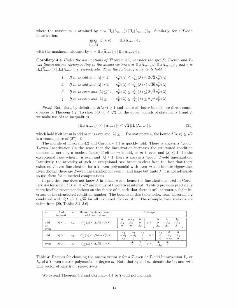
The morale of Theorem 4.2 and Corollary 4.4 is quickly told: There is always a “good”T -even linearization (in the sense that the linearization increases the structured conditionnumber at most by a modest factor) if either m is odd, or m is even and |λ| ≤ 1. In theexceptional case, when m is even and |λ| ≥ 1, there is always a “good” T -odd linearization.Intuitively, the necessity of such an exceptional case becomes clear from the fact that thereexists no T -even linearization for a T -even polynomial with even m and infinite eigenvalue.Even though there are T -even linearization for even m and large but finite λ, it is not advisableto use them for numerical computations.

In practice, one does not know λ in advance and hence the linearizations used in Corol-lary 4.4 for which δ(λ; v) ≤

√2 are mainly of theoretical interest. Table 3 provides practically

more feasible recommendations on the choice of v, such that there is still at worst a slight in-crease of the structured condition number. The bounds in this table follow from Theorem 4.2combined with δ(λ; v) ≤

√m for all displayed choices of v. The example linearizations are

taken from [29, Tables 3.4–3.6].

m λ of v Bound on struct. cond. Exampleinterest of linearization

oddoreven

|λ| ≤ 1 em κSeLe

(λ) ≤ 2√mκSe

P (λ)

24 0 −A3 0A3 A2 00 0 A0

35+ λ

24 0 0 A30 −A3 −A2A3 A2 A1

35

odd |λ| ≥ 1 e1 κSeLe

(λ) ≤√

10mκSeP (λ)

24 A2 A1 A0−A1 −A0 0A0 0 0

35+ λ

24 A3 0 00 A1 A00 −A0 0

35even |λ| ≥ 1 e1 κSo

Lo(λ) ≤ 2

√mκSe

P (λ)

»A2 00 A0

–+ λ

»A1 A0−A0 0

–

Table 3: Recipes for choosing the ansatz vector v for a T -even or T -odd linearization Le orLo of a T -even matrix polynomial of degree m. Note that e1 and em denote the 1st and mthunit vector of length m, respectively.

We extend Theorem 4.2 and Corollary 4.4 to T -odd polynomials.

14

Theorem 4.5 Let λ be a finite or infinite, simple eigenvalue of a T -odd matrix polynomialP of degree m. Then the following statements hold for ‖ · ‖M ≡ ‖ · ‖2.

1. If Lo is a T -odd linearization corresponding to the ansatz vector Σv = v then

for odd m and |λ| ≤ 1: δ(λ; v) ≤κSoLo

(λ)

κSoP (λ)

≤√

10 δ(λ; v)

for odd m and |λ| ≥ 1: δ(λ; v) ≤κSoLo

(λ)

κSoP (λ)

≤ 2 δ(λ; v)

for even m and |λ| ≤ 1: δ(λ; v) ≤κSoLo

(λ)

κSoP (λ)

≤√

10 δ(λ; v).

2. If Le is a T -even linearization corresponding to the ansatz vector v = −Σv then

for even m and |λ| ≥ 1: δ(λ; v) ≤κSeLe

(λ)

κSoP (λ)

≤√

10 δ(λ; v).

Proof. Recall that δ(λ; v) = δ(λ; Σv) holds for Σv = ±v.

1 (a). Let m be odd. Then Lemma 2.8 combined with (25) yields

κratioP,Lo(λ) =

√1− |yTx|2 1

1+|λ|2|ΛHm−1ΣΛm−1|2‖Λm−1‖42√

1− |yTx|2 ‖Πe(Λm)‖22‖Λm‖22

. (32)

Let θ = λ−1 and define Θm−1 = [θm−1, θm−2 . . . θ, 1]T . Then it is not hard to see that

κratioP,Lo(λ) = κratio

P,Lo(θ−1) =

√1− |yTx|2 |θ|2

1+|θ|2|ΘHm−1ΣΘm−1|2‖Θm−1‖42√

1− |yTx|2 ‖Πo(Θm)‖22‖Θm‖22

.

The right-hand side coincides with the starting expression (28) in the proof of Theo-rem 4.2.1 (a), only with λ replaced by θ. In particular, this implies 1 ≤ κratio

P,Lo(λ) ≤

√5

for |θ| ≥ 1 and 1 ≤ κratioP,Lo

(λ) ≤√

2 for |θ| ≤ 1.

1 (b). Let m be even and |λ| ≤ 1. Using (29), we obtain

1− 11 + |λ|2

|ΛHm−1ΣΛm−1|2

‖Λm−1‖42= 1− (1− |λ|2)2

(1 + |λ|2)3=

5|λ|2 + 2|λ|4 + |λ|6

(1 + |λ|2)3

≤ 5|λ|2(1 + |λ|2)

(1 + |λ|2)3= 5

|λ|2

(1 + |λ|2)2

(30)

≤ 5‖Πo(Λm)‖22‖Λm‖22

= 5(

1− ‖Πe(Λm)‖22‖Λm‖22

).

From (32), we therefore obtain

κratioP,Lo(λ) ≤

√1− 1

1+|λ|2|ΛHm−1ΣΛm−1|2‖Λm−1‖42√

1− ‖Πe(Λm)‖22‖Λm‖22

≤√

5.

The other direction, κratioP,Lo

(λ) ≥ 1, follows from combining (32) with ‖Πe(Λm)‖22‖Λm‖22

≥ 11+|λ|2 ,

see (27).

15

2. Now, let m be even, |λ| ≥ 1, and suppose that a T -even linearization Le is used. ThenLemmas 2.4 and 2.8 imply

κratioP,Le(λ) =

√1− |yTx|2 |λ|2

1+|λ|2|ΛHm−1ΣΛm−1|2‖Λm−1‖42√

1− |yTx|2 ‖Πe(Λm)‖22‖Λm‖22

= κratioP,Le(θ

−1) =

√1− |yTx|2 1

1+|θ|2|ΘHm−1ΣΘm−1|2‖Θm−1‖42√

1− |yTx|2 ‖Πe(Θm)‖22‖Θm‖22

and hence the result follows from 1 (b).

Corollary 4.6 Under the assumptions of Theorem 4.5, consider the specific T -odd and T -even linearizations Lo, Le corresponding to the ansatz vectors v = Πe(Λm−1)/‖Πe(Λm−1)‖2and v = Πo(Λm−1)/‖Πo(Λm−1)‖2, respectively. Then the following statements hold.

1. If m is odd and |λ| ≤ 1: κSoP (λ) ≤ κSo

Lo(λ) ≤

√20κSo

P (λ).

2. If m is odd and |λ| ≥ 1: κSoP (λ) ≤ κSo

Lo(λ) ≤ 2

√2κSo

P (λ).

3. If m is even and |λ| ≤ 1: κSoP (λ) ≤ κSo

Lo(λ) ≤

√20κSo

P (λ).

4. If m is even and |λ| ≥ 1: κSoP (λ) ≤ κSe

Le(λ) ≤

√20κSo

P (λ).

Proof. The proof is similar to that of Corollary 4.4 and follows from Theorem 4.5 and (31).

Finally, we mention that Table 3 has a corresponding analogue for a T -odd matrix polynomial.

4.3 T -palindromic matrix polynomials

Turning to (anti-)palindromic matrix polynomials, we require that a structured linearizationL satisfies (R ⊗ I)L ∈ DL(P) with the flip permutation matrix R, see (24). Again, furtherconditions need to be imposed on the ansatz vector Rv for (R⊗ I)L, see Table 4.

Structure of P Structure of L Condition on Rv

?-palindromic ?-palindromic Rv = (v?)T

?-anti-palindromic Rv = −(v?)T

?-anti-palindromic ?-palindromic Rv = −(v?)T

?-anti-palindromic Rv = (v?)T

Table 4: Conditions on ansatz vector Rv for (R ⊗ I)L ∈ DL(P) such that L is ?-(anti)-palindromic for a ?-(anti)-palindromic polynomial P. Taken from [29, Table 6.1].

As above, we obtain from Theorem 3.2

|yT x| =|ΛHm−1RΛm−1|‖Λm−1‖22

|yTx| = (m+ 1)|λ|m

‖Λm−1‖22|yTx|, (33)

where x = Λm−1 ⊗ x and y = RΛm−1 ⊗ y are the right/left eigenvectors of L correspondingto right/left eigenvectors x, y of P. Also, (26) has an (anti-)palindromic analogue:

κratioP,L (λ) · δ(λ;Rv) ≤

κSLL (λ)κSP

P (λ)≤√

2κratioP,L (λ) · δ(λ;Rv). (34)

16

This result is again instrumental for bounding the ratio between the structured eigenvaluecondition numbers for P and L.

Theorem 4.7 Let Sp and Sa denote the sets of T -palindromic and T -anti-palindromic poly-nomials, respectively. Let λ be a finite or infinite, simple eigenvalue of a T -palindromic matrixpolynomial P of degree m. Then the following statements hold for ‖ · ‖M ≡ ‖ · ‖F .

1. If Lp is a T -palindromic linearization corresponding to the ansatz vector Rv = v then

for odd m and Re(λ) ≥ 0:κ

SpLp

(λ)

κSpP (λ)

≤ 4 δ(λ; v)

for odd m and Re(λ) ≤ 0:κ

SpLp

(λ)

κSpP (λ)

≤ 2 δ(λ; v)

for even m and Re(λ) ≥ 0:κ

SpLp

(λ)

κSpP (λ)

≤ 4 δ(λ; v).

2. If La is a T -anti-palindromic linearization corresponding to the ansatz vector Rv = −vthen

for even m and Re(λ) ≤ 0:κSaLa

(λ)

κSpP (λ)

≤ 4 δ(λ; v).

Proof. Clearly, δ(λ; v) = δ(λ;Rv) for Rv = ±v.

1 (a). Let m be odd and Re(λ) ≥ 0. Lemma 2.9 together with (33) imply

κratioP,Lp(λ) =

√1 + |yTx|2 |1+λ|2−|1−λ|2

2(1+|λ|2)

|ΛHm−1RΛm−1|2‖Λm−1‖42√

1 + |yTx|2 ‖Π+(Λm)‖22−‖Π−(Λm)‖22‖Λm‖22

. (35)

For ‖Π+(Λm)‖22 ≤ ‖Π−(Λm)‖22, we obtain from Lemma B.1.1 that

κratioP,Lp(λ) ≤

√2√

1 + ‖Π+(Λm)‖22−‖Π−(Λm)‖22‖Λm‖22

=‖Λm‖2

‖Π+(Λm)‖2≤ 2√

2,

where we also used ‖Π+(Λm)‖22 +‖Π−(Λm)‖22 = ‖Λm‖22. For ‖Π+(Λm)‖22 ≥ ‖Π−(Λm)‖22,we obtain κratio

P,Lp(λ) ≤

√2 trivially from (35). Hence, the desired bound follows from (34).

1 (b). Let m be odd and Re(λ) ≤ 0. With the notation of Lemma B.1.2, the relation (35)reads

κratioP,Lp(λ) =

√1 + |yTx|2α√1 + |yTx|2β

.

Since β > −1 and |yTx| ≤ 1, the inequality α − 2β ≤ 1 shown in Lemma B.1.2 gives|yTx|2α ≤ 1 + 2|yTx|2β which is equivalent to 1+|yT x|2α

1+|yT x|2β ≤ 2. Hence the desired boundfollows from (34).

1 (c). The case of even m and Re(λ) ≥ 0 follows – analogously as in 1 (a) – from Lemma B.1.3.

2. Let m be even, Re(λ) ≤ 0, and suppose that a T -anti-palindromic linearization La isused. Then Lemma 2.9, Lemma 2.11 and (33) imply

κratioP,La(λ) =

√1− |yTx|2 |1+λ|2−|1−λ|2

2(1+|λ|2)

|ΛHm−1RΛm−1|2‖Λm−1‖42√

1 + |yTx|2 ‖Π+(Λm)‖22−‖Π−(Λm)‖22‖Λm‖22

.

17

Since the sign in the numerator is not relevant for the arguments in 1 (a) and 1 (c), theresult follows in the same way from Lemma B.1.3.

Remark 4.8 Similar to the proof of Theorem 4.7, it can be shown that the bound for anti-palindromic linearization holds for Re(λ) ≥ 0 as well, provided that m is even. Further,κratio

P,Lp(λ) ≥ 1√

2when Re(λ) ≥ 0 and κratio

P,La(λ) ≥ 1√

2when Re(λ) ≤ 0.

Motivated by the result of Theorem 4.7, a good linearization should belong to an ansatzvector that attains a small δ(λ; v) or, equivalently, a large |p(λ; v)|. By Proposition 4.3,

maxv=Rv‖v‖2≤1

|p(λ;Rv)| = ‖Π+(Λm−1)‖2,

where the maximum is attained by v+ defined as

v± =

[λm−1±1

2 , . . . , λm/2+1±λm/2

2 , λm/2+1±λm/2

2 , . . . , λm−1±1

2

]T‖Π±(Λm−1)‖2

(36)

if m is even and as

v± =

[λm−1±1

2 , . . . , λ(m−1)/2±λ(m−1)/2

2 , . . . , λm−1±1

2

]T‖Π±(Λm−1)‖2

(37)

if m is odd. Similarly,maxv=−Rv‖v‖2≤1

|p(λ;Rv)| = ‖Π−(Λm−1)‖2,

with the maximum attained by v−.

Corollary 4.9 Under the assumptions of Theorem 4.7, consider the specific T -palindromicand T -anti-palindromic linearizations Lp, La belonging to the ansatz vectors v+ and v−, re-spectively, defined in (36)–(37). Then the following statements hold.

1. If m is odd: κSpLp

(λ) ≤ 8√

2κSpP (λ).

2. If m is even and Re(λ) ≥ 0: κSpLp

(λ) ≤ 8√

2κSpP (λ).

3. If m is even and Re(λ) ≤ 0: κSaLa

(λ) ≤ 8√

2κSpP (λ).

Proof. Recall that δ(λ; v) = ‖Λm−1‖2|p(λ;v)| . All results then follow in a straightforward fashion

from Theorem 4.7 and Lemma B.1.Again, Theorem 4.7 and Corollary 4.9 admit a simple interpretation. If either m is odd

or m is even and λ has nonnegative real part, it is OK to use a T -palindromic linearization;there will be no significant increase of the structured condition number. In the exceptionalcase, when m is even and λ has negative real part, a T -anti-palindromic linearization shouldbe preferred. This is especially true for λ = −1, in which case there is no T -palindromiclinearization.

In practice, when λ is unknown, it is preferable to work with the heuristic choices listedin Table 5. The bounds listed in the table are proved in the following lemma. To providerecipes for even m larger than 2, one would need to discriminate further between |λ| close to1 and |λ| far away from 1, similarly as for odd m.

Lemma 4.10 The upper bounds on κSpLp

(λ) and κSaLa

(λ) listed in Table 5 are valid.

18

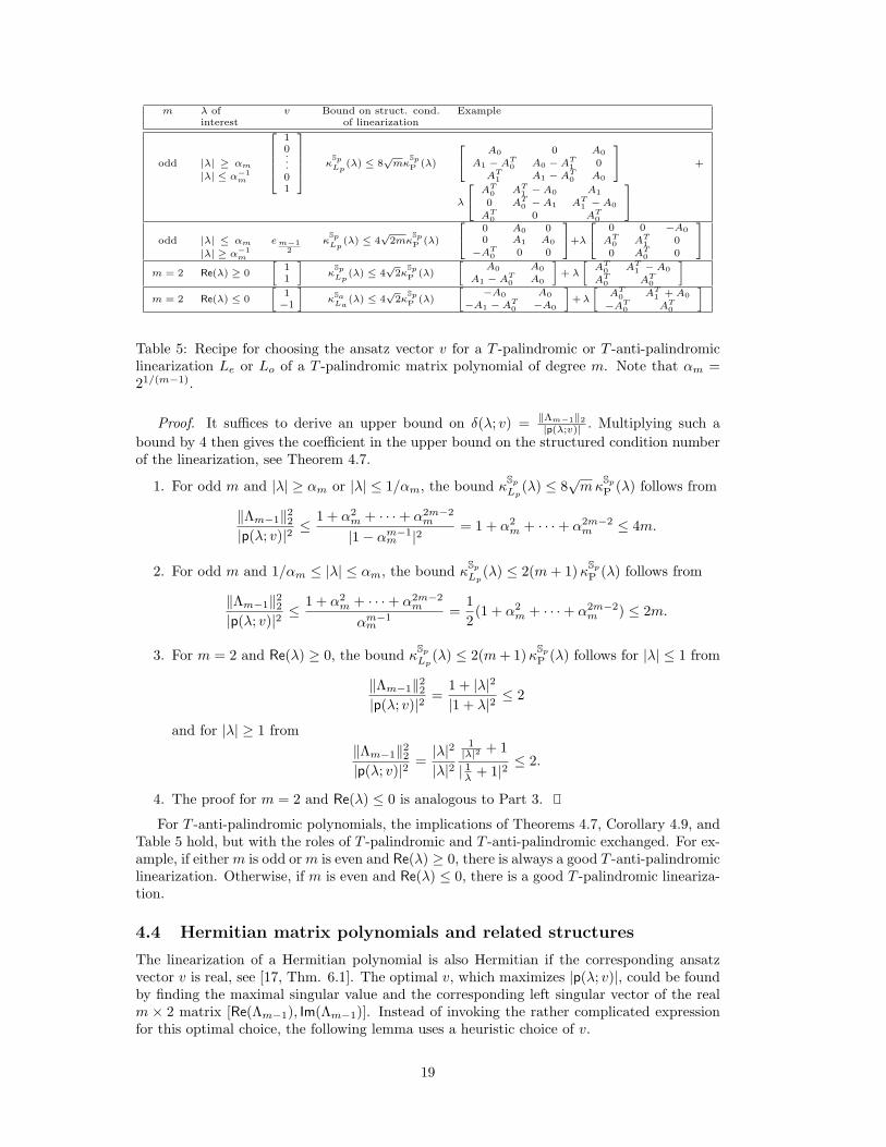
m λ of v Bound on struct. cond. Exampleinterest of linearization

odd |λ| ≥ αm|λ| ≤ α−1

m

26666410...01

377775 κSpLp

(λ) ≤ 8√mκ

SpP (λ)

24 A0 0 A0

A1 − AT0 A0 − AT1 0

AT1 A1 − AT0 A0

35 +

λ

24 AT0 AT1 − A0 A1

0 AT0 − A1 AT1 − A0

AT0 0 AT0

35odd |λ| ≤ αm

|λ| ≥ α−1m

em−12

κSpLp

(λ) ≤ 4√

2mκSpP (λ)

24 0 A0 00 A1 A0

−AT0 0 0

35+λ

24 0 0 −A0

AT0 AT1 0

0 AT0 0

35m = 2 Re(λ) ≥ 0

»11

–κ

SpLp

(λ) ≤ 4√

2κSpP (λ)

»A0 A0

A1 − AT0 A0

–+ λ

»AT0 AT1 − A0

AT0 AT0

–m = 2 Re(λ) ≤ 0

»1−1

–κSaLa

(λ) ≤ 4√

2κSpP (λ)

»−A0 A0

−A1 − AT0 −A0

–+λ

»AT0 AT1 + A0

−AT0 AT0

–

Table 5: Recipe for choosing the ansatz vector v for a T -palindromic or T -anti-palindromiclinearization Le or Lo of a T -palindromic matrix polynomial of degree m. Note that αm =21/(m−1).

Proof. It suffices to derive an upper bound on δ(λ; v) = ‖Λm−1‖2|p(λ;v)| . Multiplying such a

bound by 4 then gives the coefficient in the upper bound on the structured condition numberof the linearization, see Theorem 4.7.

1. For odd m and |λ| ≥ αm or |λ| ≤ 1/αm, the bound κSpLp

(λ) ≤ 8√mκ

SpP (λ) follows from

‖Λm−1‖22|p(λ; v)|2

≤ 1 + α2m + · · ·+ α2m−2

m

|1− αm−1m |2

= 1 + α2m + · · ·+ α2m−2

m ≤ 4m.

2. For odd m and 1/αm ≤ |λ| ≤ αm, the bound κSpLp

(λ) ≤ 2(m+ 1)κSpP (λ) follows from

‖Λm−1‖22|p(λ; v)|2

≤ 1 + α2m + · · ·+ α2m−2

m

αm−1m

=12

(1 + α2m + · · ·+ α2m−2

m ) ≤ 2m.

3. For m = 2 and Re(λ) ≥ 0, the bound κSpLp

(λ) ≤ 2(m+ 1)κSpP (λ) follows for |λ| ≤ 1 from

‖Λm−1‖22|p(λ; v)|2

=1 + |λ|2

|1 + λ|2≤ 2

and for |λ| ≥ 1 from‖Λm−1‖22|p(λ; v)|2

=|λ|2

|λ|21|λ|2 + 1

| 1λ + 1|2≤ 2.

4. The proof for m = 2 and Re(λ) ≤ 0 is analogous to Part 3.

For T -anti-palindromic polynomials, the implications of Theorems 4.7, Corollary 4.9, andTable 5 hold, but with the roles of T -palindromic and T -anti-palindromic exchanged. For ex-ample, if either m is odd or m is even and Re(λ) ≥ 0, there is always a good T -anti-palindromiclinearization. Otherwise, if m is even and Re(λ) ≤ 0, there is a good T -palindromic lineariza-tion.

4.4 Hermitian matrix polynomials and related structures

The linearization of a Hermitian polynomial is also Hermitian if the corresponding ansatzvector v is real, see [17, Thm. 6.1]. The optimal v, which maximizes |p(λ; v)|, could be foundby finding the maximal singular value and the corresponding left singular vector of the realm × 2 matrix [Re(Λm−1), Im(Λm−1)]. Instead of invoking the rather complicated expressionfor this optimal choice, the following lemma uses a heuristic choice of v.

19

Lemma 4.11 Let Sh denote the set of Hermitian polynomials. Let λ be a finite or infinite,simple eigenvalue of a Hermitian matrix polynomial P. Then the following statements holdfor ‖ · ‖M ≡ ‖ · ‖F .

1. If |λ| ≥ 1 then the linearization L corresponding to the ansatz vector v = [1, 0, . . . , 0] isHermitian and satisfies κSh

L (λ) ≤ 2√mκSh

P (λ).

2. If |λ| ≤ 1 then the linearization L corresponding to the ansatz vector v = [0, . . . , 0, 1] isHermitian and satisfies κSh

L (λ) ≤ 2√mκSh

P (λ).

Proof. Assume |λ| ≥ 1. Lemma 2.12 together with Lemma 3.3 and (21) imply

κShL (λ)κSh

P (λ)≤√

2κLp(λ)κP(λ)

=√

2‖Λm−1‖2|p(λ; v)|

≤ 2√m|λ|m

|λ|m= 2√m.

The proof for |λ| ≤ 1 proceeds analogously.H-even and H-odd matrix polynomials are closely related to Hermitian matrix polyno-

mials, see Remark 2.13. In particular, Lemma 4.11 applies verbatim to H-even and H-oddpolynomials. Note, however, that in the case of even m the ansatz vector v = [1, 0, . . . , 0]yields an H-odd linearization for an H-even polynomial, and vice versa. Similarly, the recipesof Table 5 can be extended to H-palindromic polynomials.

5 Summary and conclusions

We have derived relatively simple expressions for the structured eigenvalue condition numbersof certain structured matrix polynomials. These expressions have been used to analyze thepossible increase of the condition numbers when the polynomial is replaced by a structuredlinearization. At least in the case when all coefficients of the polynomial are perturbed to thesame extent, the result is very positive: There is always a structured linearization such thatthe condition numbers increase at most by a factor linearly depending on m. We have alsoprovided recipes for structured linearizations, which do not depend on the exact value of theeigenvalue, and for which the increase of the condition number is still negligible. Hence, theaccuracy of a strongly backward stable eigensolver applied to the structured linearization willfully enjoy the benefits of structure on the sensitivity of an eigenvalue for the original matrixpolynomial.

6 Acknowledgments

The authors thank Shreemayee Bora for inspiring discussions on the subject of this paperand the referees for their constructive remarks. Parts of this work was performed while thefirst author was staying at ETH Zurich. The financial support by the Indo Swiss BilateralResearch Initiative (ISBRI), which made this visit possible, is gratefully acknowledged.

References

[1] S. S. Ahmad. Pseudospectra of Matrix Pencils and Their Applications in PerturbationAnalysis of Eigenvalues and Eigendecompositions. PhD thesis, Department of Mathe-matics, IIT Guhawati, India, 2007.

[2] S. S. Ahmad and R. Alam. Pseudospectra, critical points and multiple eigenvalues ofmatrix polynomials. Linear Algebra Appl., 430:1171–1195, 2009.

[3] A. L. Andrew, E. K.-W. Chu, and P. Lancaster. Derivatives of eigenvalues and eigenvec-tors of matrix functions. SIAM J. Matrix Anal. Appl., 14(4):903–926, 1993.

20

[4] F. S. V. Bazan. Eigenvalues of Matrix Polynomials, Sensitivity, Computation and Ap-plications (in Portuguese). IMPA, Rio de Janeiro, Brazil, 2003.

[5] M. Berhanu. The Polynomial Eigenvalue Problem. PhD thesis, School of Mathematics,The University of Manchester, UK, 2005.

[6] T. Betcke. Optimal scaling of generalized and polynomial eigenvalue problems. SIAM J.Matrix Anal. Appl., 30(4):1320–1338, 2008.

[7] S. Bora. Structured eigenvalue condition number and backward error of a class of poly-nomial eigenvalue problems. SIAM J. Matrix Anal. Appl., 31(3):900–917, 2009.

[8] R. Byers and D. Kressner. On the condition of a complex eigenvalue under real pertur-bations. BIT, 44(2):209–215, 2004.

[9] E. K.-W. Chu. Perturbation of eigenvalues for matrix polynomials via the Bauer-Fiketheorems. SIAM J. Matrix Anal. Appl., 25(2):551–573, 2003.

[10] J.-P. Dedieu and F. Tisseur. Perturbation theory for homogeneous polynomial eigenvalueproblems. Linear Algebra Appl., 358:71–94, 2003.

[11] H.-Y. Fan, W.-W. Lin, and P. Van Dooren. Normwise scaling of second order polynomialmatrices. SIAM J. Matrix Anal. Appl., 26(1):252–256, 2004.

[12] T. W. Gamelin and R. E. Greene. Introduction to Topology. Dover, Mineola, NY, secondedition, 1999.

[13] G. H. Golub and C. F. Van Loan. Matrix Computations. Johns Hopkins University Press,Baltimore, MD, third edition, 1996.

[14] D. J. Higham and N. J. Higham. Structured backward error and condition of generalizedeigenvalue problems. SIAM J. Matrix Anal. Appl., 20(2):493–512, 1999.

[15] N. J. Higham. Accuracy and Stability of Numerical Algorithms. SIAM, Philadelphia, PA,second edition, 2002.

[16] N. J. Higham, R.-C. Li, and F. Tisseur. Backward error of polynomial eigenproblemssolved by linearization. SIAM J. Matrix Anal. Appl., 29(4):1218–1241, 2007.

[17] N. J. Higham, D. S. Mackey, N. Mackey, and F. Tisseur. Symmetric linearizations formatrix polynomials. SIAM J. Matrix Anal. Appl., 29(1):143–159, 2007.

[18] N. J. Higham, D. S. Mackey, and F. Tisseur. The conditioning of linearizations of matrixpolynomials. SIAM J. Matrix Anal. Appl., 28(4):1005–1028, 2006.

[19] N. J. Higham, D. S. Mackey, F. Tisseur, and S. D. Garvey. Scaling, sensitivity andstability in the numerical solution of quadratic eigenvalue problems. Internat. J. Numer.Methods Engrg., 73(3):344–360, 2008.

[20] A. Hilliges, C. Mehl, and V. Mehrmann. On the solution of palindromic eigenvalueproblems. In Proceedings of ECCOMAS, Jyvaskyla, Finland, 2004.

[21] M. Karow. µ-values and spectral value sets for linear perturbation classes defined by ascalar product, 2007. Submitted.

[22] M. Karow. Structured pseudospectra and the condition of a nonderogatory eigenvalue,2007. Submitted.

[23] M. Karow, D. Kressner, and F. Tisseur. Structured eigenvalue condition numbers. SIAMJ. Matrix Anal. Appl., 28(4):1052–1068, 2006.

21

[24] D. Kressner, M. J. Pelaez, and J. Moro. Structured Holder condition numbers for multipleeigenvalues. SIAM J. Matrix Anal. Appl., 31(1):175–201, 2009.

[25] A. Kurzhanski and I. Valyi. Ellipsoidal calculus for estimation and control. Systems &Control: Foundations & Applications. Birkhauser Boston Inc., Boston, MA, 1997.

[26] P. Lancaster, A. S. Markus, and F. Zhou. Perturbation theory for analytic matrix func-tions: the semisimple case. SIAM J. Matrix Anal. Appl., 25(3):606–626, 2003.

[27] H. Langer and B. Najman. Remarks on the perturbation of analytic matrix functions.II. Integral Equations Operator Theory, 12(3):392–407, 1989.

[28] H. Langer and B. Najman. Leading coefficients of the eigenvalues of perturbed analyticmatrix functions. Integral Equations Operator Theory, 16(4):600–604, 1993.

[29] D. S. Mackey, N. Mackey, C. Mehl, and V. Mehrmann. Structured polynomial eigen-value problems: good vibrations from good linearizations. SIAM J. Matrix Anal. Appl.,28(4):1029–1051, 2006.

[30] D. S. Mackey, N. Mackey, C. Mehl, and V. Mehrmann. Vector spaces of linearizationsfor matrix polynomials. SIAM J. Matrix Anal. Appl., 28(4):971–1004, 2006.

[31] V. Mehrmann and H. Xu. Perturbation of purely imaginary eigenvalues of Hamiltonianmatrices under structured perturbations. Electron. J. Linear Algebra, 17:234–257, 2008.

[32] S. Noschese and L. Pasquini. Eigenvalue condition numbers: zero-structured versustraditional. J. Comput. Appl. Math., 185(1):174–189, 2006.

[33] S. M. Rump. Eigenvalues, pseudospectrum and structured perturbations. Linear AlgebraAppl., 413(2-3):567–593, 2006.

[34] G. W. Stewart and J.-G. Sun. Matrix Perturbation Theory. Academic Press, New York,1990.

[35] F. Tisseur. Backward error and condition of polynomial eigenvalue problems. LinearAlgebra Appl., 309(1-3):339–361, 2000.

A Derivation of results given in Section 2

This section contains the proofs of the results on structured eigenvalue condition numbersgiven in Section 2. As mentioned before, the starting point to derive explicit expressions forstructured eigenvalue condition number is the formulation (12).

A.1 Structured first-order perturbation sets

To proceed from the characterization (12) of the structured eigenvalue condition number, weneed to find the maximal absolute magnitude of elements from the set{

yH4P(λ)x = yHE0x+ λyHE1x+ · · ·λmyHEmx : 4P ∈ S, ‖4P‖ ≤ 1}

(38)

It is therefore of interest to study the nature of the set {yHEx : E ∈ E, ‖E‖M ≤ 1} withrespect to some E ⊆ Cn×n. The following theorem by Karow [21] provides explicit descriptionsof this set for certain E. Note that the symbol ∼= is used to denote the natural isomorphismbetween C and R2.

22

Theorem A.1 Let K(E, x, y) := {yHEx : E ∈ E, ‖E‖M ≤ 1} for x, y ∈ Cn with ‖x‖2 =‖y‖2 = 1 and some E ⊆ Cn×n. Provided that ‖ · ‖M ∈ {‖ · ‖2, ‖ · ‖F }, the set K(E, x, y) is anellipse taking the form

K(E, x, y) ∼= K(α, β) :={K(α, β)ξ : ξ ∈ R2, ‖ξ‖2 ≤ 1

}, K(α, β) ∈ R2×2, (39)

for the cases that E consists of all complex (E = Cn×n), real (E = Rn×n), Hermitian(E = Herm), complex symmetric (E = symm), and complex skew-symmetric (E = skew),real symmetric (only for ‖ · ‖M ≡ ‖ · ‖F ), and real skew-symmetric matrices. The matrixK(α, β) defining the ellipse in (39) can be written as

K(α, β) =[

cosφ/2 sinφ/2− sinφ/2 cosφ/2

] [ √α+ |β| 0

0√α− |β|

](40)

with some of the parameter configurations α, β listed in Table 6, and φ = arg(β).

‖ · ‖M ≡ ‖ · ‖2 ‖ · ‖M ≡ ‖ · ‖FE α β α β

Cn×n 1 0 1 0Herm 1− 1

2 |yHx|2 1

2 (yHx)2 12

12 (yHx)2

symm 1 0 12 (1 + |yTx|2) 0

skew 1− |yTx|2 0 12 (1− |yTx|2) 0

Table 6: Parameters defining the ellipse (39).

Note that (39)–(40) describes an ellipse with semiaxes√α+ |β|,

√α− |β|, rotated by the

angle φ/2. The Minkowski sum of ellipses is still convex but in general not an ellipse [25].Finding the maximal element in (38) is equivalent to finding the maximal element in theMinkowski sum.

Lemma A.2 Let K(α0, β0), . . . ,K(αm, βm) be ellipses of the form (39)–(40). Define

σ := supb0,...,bm∈Rb20+···+b2m≤1

sup{‖s‖2 : s ∈ b0K(α0, β0) + · · ·+ bmK(αm, βm)

}(41)

using the Minkowski sum of sets. Then

σ = ‖[K(α0, β0), . . . ,K(αm, βm)]‖2, (42)

and √α0 + · · ·+ αm ≤ σ ≤

√2√α0 + · · ·+ αm. (43)

Proof. By the definition of K(αj , βj), it holds that

σ = supbi∈R

b20+···+b2m≤1

supξi∈R2

‖ξi‖2≤1

∥∥b0K(α0, β0)ξ0 + · · ·+ bmK(αm, βm)ξm∥∥

2

= supbi∈R

b20+···+b2m≤1

supξi∈R2

‖ξi‖2≤bi

∥∥K(α0, β0)ξ0 + · · ·+K(αm, βm)ξm∥∥

2

= supξi∈R2

‖ξ0‖22+···+‖ξm‖22≤1

∥∥K(α0, β0)ξ0 + · · ·+K(αm, βm)ξm∥∥

2

=∥∥[K(α0, β0), . . . , K(αm, βm)

]∥∥2,

23

applying the definition of the matrix 2-norm. The inequality (43) then follows from thewell-known bound

1√2‖[K(α0, β0), . . . ,K(αm, βm)]‖F ≤ σ ≤ ‖[K(α0, β0), . . . ,K(αm, βm)]‖F

and using the fact that:

‖[K(α0, β0), . . . ,K(αm, βm)]‖2F =m∑i=0

‖K(αi, βi)‖2F =m∑i=0

2αi.

It is instructive to rederive the expression (10) for the unstructured condition number fromLemma A.2. Starting from Equation (7), we insert the definition (4) of ‖4P‖ for ‖·‖M ≡ ‖·‖2,‖ · ‖V ≡ ‖ · ‖2, and obtain

σP(λ) := sup{|yH4P(λ)x| : ‖4P‖ ≤ 1

}= sup

b20+···+b2m≤1

‖E0‖2≤b0,...,‖Em‖2≤bm

∣∣∣ m∑i=0

ωiλiyHEix

∣∣∣= sup

b20+···+b2m≤1

sup{|s| : s ∈

m∑i=0

biωiλiK(Cn×n, x, y)}. (44)

By Theorem A.1, K(Cn×n, x, y) ∼= K(1, 0) and, since a disk is invariant under rotation,ωiλ

iK(Cn×n, x, y) ∼= K(ω2i |λ|2i, 0). Applying Lemma A.2 yields

σP(λ) =∥∥[K(ω2

0 , 0),K(ω21 |λ|2, 0), . . . ,K(ω2

m|λ|2m, 0)]∥∥

2=∥∥[ω0, ω1λ, . . . , ωmλ

m]∥∥

2,

which together with (7) results in the known expression (10) for κP(λ).In the following, it will be shown that expressions for structured condition numbers follow

in a similar way from Lemma A.2. To keep the notation compact, we define

σSP(λ) = sup

{|yH4P(λ)x| : 4P ∈ S, ‖4P‖ ≤ 1

}.

for a star-shaped set S. By (12), κSP(λ) = σS

P(λ)/|yHP′(λ)x|.

A.2 Proofs

Proof of Lemma 2.3 (S = complex symmetric matrix polynomials) Along the lineof arguments leading to (44),

σSP(λ) = sup

b20+···+b2m≤1

{|s| : s ∈

m∑i=0

biωiλiK(symm, x, y)

}for finite λ. As in the unstructured case, K(symm, x, y) ∼= K(1, 0) for ‖ · ‖M ≡ ‖ · ‖2 byTheorem A.1, and thus κP(λ) = κS

P(λ). For ‖ · ‖M ≡ ‖ · ‖F we have

K(symm, x, y) ∼= K((1 + |yTx|2)/2, 0) =

√1 + |yTx|2√

2K(1, 0),

showing the second part of the statement. The proof for infinite λ is entirely analogous.

24

Proof of Lemma 2.4 (S = T -even matrix polynomials) By definition, the even coef-ficients of a T -even polynomial are symmetric while the odd coefficients are skew-symmetric.Thus, for finite λ,

σSP(λ) = sup

b20+···+b2m≤1

sup{|s| : s ∈

∑i even

biωiλiK(symm, x, y) +

∑i odd

biωiλiK(skew, x, y)

}.

Applying Theorem A.1 and Lemma A.2 yields for ‖ · ‖M ≡ ‖ · ‖2,

σSP(λ) =

∥∥∥[Πe(Λω)T ⊗K(1, 0), Πo(Λω)T ⊗K(1− |yTx|2, 0)]∥∥∥

2

=∥∥∥[Πe(Λω)T ,

√1− |yTx|2Πo(Λω)T

]∥∥∥2

=√‖Λω‖22 − |yTx|2‖Πo(Λω)‖22,

once again using the fact that a disk is invariant under rotation. Similarly, it follows for‖ · ‖M ≡ ‖ · ‖F that

σSP(λ) =

1√2

∥∥∥[√1 + |yTx|2Πe(Λω)T ,√

1− |yTx|2Πo(Λω)T]∥∥∥

2

=1√2

√‖Λω‖22 + |yTx|2

(‖Πe(Λω)‖22 − ‖Πo(Λω)‖22

).

The result for infinite λ follows in an analogous manner.

Proof of Lemma 2.9 (S = T -palindromic matrix polynomials) Assume m is odd.For 4P ∈ S,

4P(λ) =(m−1)/2∑i=0

λiEi +(m−1)/2∑i=0

λm−iETi

=(m−1)/2∑i=0

λi + λm−i√2

Ei + ETi√2

+(m−1)/2∑i=0

λi − λm−i√2

Ei − ETi√2

.

Let us introduce the auxiliary polynomial

4P(µ) =(m−1)/2∑i=0

µ2iSi +(m−1)/2∑i=0

µ2i+1Wi, Si =Ei + ETi√

2, Wi =

Ei − ETi√2

.

Then P ∈ S, where S denotes the set of T -even polynomials. Since symmetric and skew-symmetric matrices are orthogonal to each other with respect to the matrix inner product〈A,B〉 = trace(BHA), we have ‖A‖2F + ‖AT ‖2F = ‖(A + AT )/

√2‖2F + ‖(A − AT )/

√2‖2F for

25

any A ∈ Cn×n and hence ‖4P‖ = ‖4P‖ for ‖ · ‖M ≡ ‖ · ‖F . This allows us to write

σSP(λ) = sup

{|yH4P(λ)x| : 4P ∈ S, ‖4P‖ ≤ 1

}= sup

{∣∣∣∣∑ λi + λm−i√2

yHSix+∑ λi − λm−i√

2yHWix

∣∣∣∣ : 4P ∈ S, ‖4P‖ ≤ 1}

=1√2

supb20+···+b2m≤1

{|s| : s ∈

∑biωi(λi + λm−i)K(symm, x, y)

+∑

b(m−1)/2+iωi(λi − λm−i)K(skew, x, y)}

=12

√(1 + |yTx|2)

∑ω2i |λi + λm−i|2 + (1− |yTx|2)

∑ω2i |λi − λm−i|2

=1√2

√(1 + |yTx|2)‖Π+(Λω)‖22 + (1− |yTx|2)‖Π−(Λω)‖22

=1√2

√‖Λω‖22 + |yTx|2(‖Π+(Λω)‖22 − ‖Π−(Λω)‖22),

where we used Theorem A.1 and Lemma A.2.For even m the proof is almost identical; with the only difference that the transformation

leaves the complex symmetric middle coefficient Am/2 unaltered.For λ = ∞, observe that the corresponding optimization problem (13) involves only a

single, unstructured coefficient of the polynomial and hence palindromic structure has noeffect on the condition number.

The derivations above were greatly simplified by the fact that the first-order perturbationsets under consideration were disks. For the set of Hermitian perturbations, however, yHEixforms truly an ellipse. Still, a computable expression is provided by (42) from Lemma A.2.However, the explicit formulas derived from this expression take a very technical form andprovide little immediate intuition on the difference between the structured and unstructuredcondition number. Therefore, the result of Lemma 2.12 is based on the bound (43) instead.

Proof of Lemma 2.12 (S = Hermitian matrix polynomials) Let ‖ · ‖M ≡ ‖ · ‖F . ThenTheorem A.1 states

K(Herm, x, y) ∼= K(1/2, (yHx)2/2).

Consequently,ωiλ

iK(Herm, x, y) ∼= K(ω2i |λ|2i/2, ω2

i λ2i(yHx)2/2),

which implies

σSP(λ) = sup

b20+···+b2m≤1

{‖s‖2 : s ∈

m∑i=0

biK(ω2i λ

2i/2, ω2i λ

2i(yHx)2/2)}.

By Lemma A.2,1√2‖Λω‖2 ≤ σS

P(λ) ≤ ‖Λω‖2.

The proof for the case ‖ · ‖M ≡ ‖ · ‖2 is analogous.

B Auxiliary results for T -palindromic matrix polynomi-als

The following lemma summarizes some auxiliary results needed in the proofs given in Sec-tion 4.3 concerning the condition number growth for linearizations of T -palindromic matrixpolynomials.

26

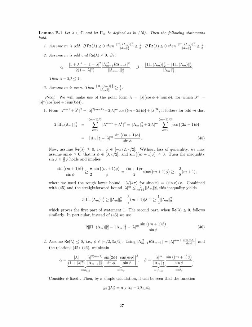
Lemma B.1 Let λ ∈ C and let Π± be defined as in (16). Then the following statementshold.

1. Assume m is odd. If Re(λ) ≥ 0 then ‖Π+(Λm)‖22‖Λm‖22

≥ 18 . If Re(λ) ≤ 0 then ‖Π−(Λm)‖22

‖Λm‖22≥ 1

8 .

2. Assume m is odd and Re(λ) ≤ 0. Set

α =|1 + λ|2 − |1− λ|2

2(1 + |λ|2)|ΛHm−1RΛm−1|2

‖Λm−1‖42, β =

‖Π+(Λm)‖22 − ‖Π−(Λm)‖22‖Λm‖22

.

Then α− 2β ≤ 1.

3. Assume m is even. Then ‖Π+(Λm)‖22‖Λm‖22

≥ 18 .

Proof. We will make use of the polar form λ = |λ|(cosφ + i sinφ), for which λk =|λ|k(cos(kφ) + i sin(kφ)).

1. From |λm−k+λk|2 = |λ|2(m−k) +2|λ|m cos((m−2k)φ

)+ |λ|2k, it follows for odd m that

2‖Π+(Λm)‖22 =(m−1)/2∑k=0

|λm−k + λk|2 = ‖Λm‖22 + 2|λ|m(m−1)/2∑k=0

cos((2k + 1)φ

)= ‖Λm‖22 + |λ|m

sin((m+ 1)φ

)sinφ

. (45)

Now, assume Re(λ) ≥ 0, i.e., φ ∈ [−π/2, π/2]. Without loss of generality, we mayassume sinφ ≥ 0, that is φ ∈ [0, π/2], and sin

((m + 1)φ

)≤ 0. Then the inequality

sinφ ≥ 2πφ holds and implies

sin((m+ 1)φ

)sinφ

≥ π

2sin((m+ 1)φ

)φ

=(m+ 1)π

2sinc

((m+ 1)φ

)≥ −3

8(m+ 1),

where we used the rough lower bound −3/(4π) for sinc(x) = (sinx)/x. Combinedwith (45) and the straightforward bound |λ|m ≤ 2

m+1‖Λm‖22, this inequality yields

2‖Π+(Λm)‖22 ≥ ‖Λm‖22 −38

(m+ 1)|λ|m ≥ 14‖Λm‖22

which proves the first part of statement 1. The second part, when Re(λ) ≤ 0, followssimilarly. In particular, instead of (45) we use

2‖Π−(Λm)‖22 = ‖Λm‖22 − |λ|msin((m+ 1)φ

)sinφ

. (46)

2. Assume Re(λ) ≤ 0, i.e., φ ∈ [π/2, 3π/2]. Using |ΛHm−1RΛm−1| = |λ|m−1∣∣∣ sin(mφ)

sinφ

∣∣∣ andthe relations (45)–(46), we obtain

α =|λ|

(1 + |λ|2)|λ|2(m−1)

‖Λm−1‖42︸ ︷︷ ︸=:α|λ|

sin(2φ)sinφ

∣∣∣∣ sin(mφ)sinφ

∣∣∣∣2︸ ︷︷ ︸=:αφ

, β =|λ|m

‖Λm‖22︸ ︷︷ ︸=:β|λ|

sin((m+ 1)φ

)sinφ︸ ︷︷ ︸=:βφ

.

Consider φ fixed . Then, by a simple calculation, it can be seen that the function

gφ(|λ|) = α|λ|αφ − 2β|λ|βφ

27

tends to zero for |λ| → 0 and |λ| → ∞. Moreover, gφ(|λ|) is either completely zero orhas precisely one extremum at |λ| = 1. Hence, gφ(|λ|) is bounded from above by themaximum between zero and its value at 1:

gφ(1) =sin(2φ)2 sinφ

∣∣∣∣ sin(mφ)m sinφ

∣∣∣∣2 − 2sin((m+ 1)φ

)(m+ 1) sinφ

.

The maximal value of gφ(1) is attained at φ = π, for which gπ(1) = 1. This proves thedesired result.

3. As in part 1, the expression

2‖Π+(Λm)‖22 = ‖Λm‖22 + |λ|msin((m+ 1)φ

)sinφ

can be shown to also hold for even m. As above, we have

sin((m+ 1)φ

)sinφ

≥ −38

(m+ 1), for φ ∈ [−π/2, π/2]. (47)

Combined with the straightforward bound |λ|m ≤ 2m+2‖Λm‖

22 ≤ 2

m+1‖Λm‖22, this shows

the lower bound when Re(λ) ≥ 0, as in part 1. It remains to discuss the case Re(λ) ≤ 0,that is φ ∈ [π/2, 3π/2]. Since m is even, it follows for φ := φ−π ∈ [−π/2, π/2] from (47)that

sin((m+ 1)φ

)sinφ

=− sin

((m+ 1)φ

)− sin φ

=sin((m+ 1)φ

)sin φ

≥ −38

(m+ 1).

The desired lower bound follows from this inequality as above.

28