Segmentation of white matter lesions from multimodal MRI in

small vessel disease

Ana Isabel da Silva Loução Graça

Dissertation to obtain the Master of Science Degree in Biomedical Technologies

Mestrado Bolonha em Tecnologias Biomédicas

Supervisor: Prof. Patrícia Margarida Piedade Figueiredo

Dr. Pedro Ferro Vilela

Jury

Chairperson: Prof. Ana Luísa Nobre Fred

Supervisor: Prof. Patrícia Margarida Piedade Figueiredo

Members of the Committee: Prof. Rita Homem de Gouveia Costanzo Nunes

December 2016

Adoramos a perfeição, porque não a podemos ter;

repugna-la-íamos, se a tivéssemos.

O perfeito é desumano porque o humano é imperfeito

Bernardo Soares

in Livro do Desassossego

Acknowledgements

Over these last months some people had a fundamental role to the success of this dissertation.

Firstly I have to thank my supervisor, Prof. Patrícia Figueiredo, for all the kindness that she

demonstrated when accepting to work with me in the middle of the semester. Also, it is important do not

forget all the help that she gave me and the patience that she had during all this process.

I would also like to thank to Dr. Pedro Vilela. All the remarks that he gave, promoted more correct

results based on the clinical experience.

I would like to thank Joana Pinto for the fundamental tips that helped a lot in some steps. I think

that without them I would have a lot of difficulties to get to some conclusions.

To my parents, Lurdes and António, my brother Carlos and my aunt Paula that are always present

and understand all my bad moods and my absence for these last months.

Special thanks to Sandra Raquel Rodrigues, João Roma, Marisa Cruz and Nuno Antunes for all

the support, not only psychological but also for all the help that they gave me to write this thesis in a much

proper English. It is important to mention other friends that are always there for me, even when my

absence last for months. This thanks goes to Joana Oliveira, Constantino Santos, Ricardo Carvalho, Sara

Martins, Tiago Fernandes, Cristiana Alves, André Rodrigues, Vilma Franco, Nuno Rodrigues, António

Antunes.

I would like to thank to my nuclear medicine co-workers António Vieira Marques and Eduarda

Silva that always try to relieve me from some work in the nuclear medicine department and gave me full

support during this process.

To all my friends that show me that I am capable to overtake all the problems and finish this

dissertation in time. All these people show me that we are not alone and friendship is fundamental if we

want to accomplish our life objectives, especially, our dreams.

Thank you all!

Abstract

Cerebral Small Vessels Disease (SVD) is one of the main causes of cognitive impairment.

Magnetic Resonance Image (MRI) has a high diagnostic and prognostic value for this kind of pathology.

White matter lesions (WML) are one of the disease characteristic lesion types, which are most robustly

detected as hyperintensities on images acquired using Fluid Attenuation Inversion Recovery (FLAIR) MRI.

The WML load has high clinical relevance, and it is usually evaluated using qualitative scales by the

neuroradiologist. However, a clear correlation cannot be found between WML load evaluated using these

scales and disease progression. It would therefore been desirable to perform the segmentation of the

WML’s and subsequently quantify their volume. However, although several studies have addressed this

issue, there is yet no standard, automatic method for WML segmentation.

In this work, we propose an automatic WML segmentation methodology, which is based on the

use of a common tissue segmentation algorithm available on a freeware software package for image

processing – FSL – applied to multimodal MRI acquisitions, namely a FLAIR image and a T1-weighted

image (T1-W). After pre-processing, the FAST algorithm was used for tissue segmentation into three

tissue classes with a multi-channel approach taking both the FLAIR and T1-W images as input. Both

images were co-registration to the standard MNI, and the white matter (WM) mask obtained by tissue

segmentation of the MNI standard T1-W image was subtracted from the WM mask obtained by the

individual tissue segmentation in each patient: the difference between these two WM masks should

correspond to the WML’s in each patient.

The proposed methodology was applied to images collected from a group of 16 patients with

SVD. Sensitivity, specificity and accuracy were computed for each patient, through comparison with the

ground truth obtained by manual segmentation of the WMLs. The Dice coefficient between the automatic

and manual segmentation results was also computed. The average results belong to the best parameter

set and were: sensitivity 40,73%; specificity 95,33%; Dice coefficient 0,23.

In summary, our proposed methodology, relying on standard and freeware tissue segmentation

and co-registration tools, was able to achieve a WML segmentation with good sensitivity, specificity, and it

may therefore yield a useful approach to WML quantification in SVD. Future work should investigate

whether WML quantification obtained in this way may contribute a useful biomarker of SVD.

Key-words: Small Vessels Disease, White Matter Lesion, FLAIR, Segmentation, FSL

Resumo

A Doença dos Pequenos Vasos (SVD) do cérebro é uma das principais causas de défice

cognitivo. A imagem de Ressonância Magnética (MRI) tem um alto valor de diagnóstico e de prognóstico

para esta patologia. As lesões da substância branca são lesões características da SVD e podem ser

detetadas através do hiper sinal das imagens da Fluid Attenuation Inversion Recovery (FLAIR) na MRI. A

carga de lesões da substância branca tem relevância clínica. Esta é habitualmente avaliada através do

uso de escalas qualitativas por neurorradiologistas. Contudo, não existe uma correlação clara entre a

carga das WML e a progressão da doença. Assim, pode ser preferível realizar a segmentação da WML e

depois quantificar o seu volume. Apesar de vários estudos abordarem este assunto, não existe ainda um

método automático padrão de segmentar as WML.

Este trabalho apresenta uma metodologia de segmentação automática das WML. Esta tem por

base o algoritmo de segmentação de tecidos existente no software livre de processamento de imagem –

FSL – aplicando aquisições multimodais (imagem FLAIR e imagem T1-ponderado (T1-W)). Após o pré-

processamento, utilizou-se o algoritmo FAST para a segmentação dos tecidos em três classes utilizando

múltiplos canais, ou seja as imagens do FLAIR e do T1-W como entradas. Ambas as imagens estão co-

registadas com o padrão (MNI). As máscaras da substância branca foram obtidas através da

segmentação da imagem do MNI que foi, por sua vez, subtraída à máscara obtida através da

segmentação dos tecidos em cada doente. A diferença entre estas duas máscaras corresponde à WML

de cada doente.

A metodologia proposta foi aplicada às imagens adquiridas de um grupo de 16 doentes com

SVD. A sensibilidade, especificidade e exatidão foram calculadas para cada doente e comparadas com

um padrão das lesões obtido através da segmentação manual das WML. O coeficiente de Dice foi

calculado através da comparação deste padrão manual com a segmentação automática. A média dos

resultados apresentada pertence ao conjunto de parâmetros mais viável: sensibilidade 40,73%;

especificidade 95,33%; coeficiente de Dice 0,23.

A metodologia proposta tem por base a utilização de ferramentas de segmentação e co-registo

de uso livre. Estas permitiram alcançar resultados razoáveis em relação à sensibilidade e especificidade,

podendo ser, futuramente, uma abordagem útil na quantificação da SVD. Para trabalhos futuros pode ser

importante investigar a quantificação da WML de modo a obter um possível biomarcador das SVD.

Palavras-chave: Doença dos pequenos vasos, Lesões da matéria branca, FLAIR, Segmentação, FSL

Contents

Chapter 1 – Introdution .................................................................................................................... 1

1.1. Small Vessel Disease............................................................................................................. 1

1.2. Magnetic Resonance Imaging ................................................................................................ 3

1.2.1. Basic Principles .............................................................................................................. 3

1.2.2. T1-Weighted imaging ...................................................................................................... 5

1.2.3. T2-Weighted imaging ...................................................................................................... 6

1.2.4. Inversion recovery .......................................................................................................... 6

1.2.5. MRI in SVD..................................................................................................................... 7

1.3. Lesion segmentation .............................................................................................................. 9

1.3.1. Lesion segmentation in SVD ......................................................................................... 10

1.4. Goals and outline ................................................................................................................. 12

Chapter 2 – Methodology ............................................................................................................... 14

2.1. Study Population ............................................................................................................... 14

2.2. Acquisition Protocol .............................................................................................................. 14

2.3. Image Processing ................................................................................................................ 15

2.3.1. Pre-processing: skull stripping ...................................................................................... 15

2.3.2. Image registration ......................................................................................................... 15

2.3.3. Tissue segmentation ..................................................................................................... 17

2.3.4. Lesion segmentation ..................................................................................................... 18

2.4. Performance Evaluation ....................................................................................................... 18

Chapter 3 – Results ....................................................................................................................... 20

3.1. Pre-processing: skull stripping .............................................................................................. 20

3.2. Image registration ................................................................................................................ 21

3.3. Tissue segmentation ............................................................................................................ 23

3.4. Lesion segmentation ............................................................................................................ 23

Chapter 4 – Discussion .................................................................................................................. 37

Chapter 5 – Conclusion .................................................................................................................. 41

References .................................................................................................................................... 42

List of Figures

Figure 1: Different sequences based on TE and TR [14] .......................................................................... 6

Figure 2: FLAIR sequence image [14] ..................................................................................................... 7

Figure 3: WML present in T1-W and FLAIR image ................................................................................... 8

Figure 4: Skull stripping. Comparative image before and after FLAIR application. In A it was observed a

region that do not belong to brain tissue (arrow). In B the BET tool do not contemplate some brain tissue

(arrow). .................................................................................................................................................. 20

Figure 5: Registration results. Comparison between FLIRT registrations. A – FLAIR; B - WM from T1-W to

FLAIR registration with FLIRT and DOF 6 ; C - WM from T1-W to FLAIR registration with FLIRT and DOF

12; D – Overlap of WM from FLIRT DOF 12 and FLIRT DOF 6............................................................. 21

Figure 6: Registration results. Comparison between the WM from different registrations. A - WM from T1-

W to FLAIR registration with FLIRT DOF12; D - WM from MNI to FLAIR registration with FLIRT DOF 12; C

- WM from MNI to FLAIR registration with FNIRT ; D - WM from MNI to FLAIR registration with FNIRT with

lambda=8; E – Comparison between WM T1-W to FLAIR registration and WM MNI to FLAIR registration

with FLIRT DOF 12; F – Comparison between WM T1-W to FLAIR registration and WM MNI to FLAIR

registration with FNIRT; G – Comparison between WM T1-W to FLAIR registration and WM MNI to FLAIR

registration with FNIRT lambda=8; H - Comparison between WM MNI to FLAIR registration to FNIRT and

WM MNI to FLAIR registration with FNIRT lambda=8. ............................................................................ 22

Figure 7: Segmentation Results: A – FLAIR image; B –FLAIR segmentation in 3 classes; C - FLAIR

segmentation in 4 classes; D – FLAIR and T1-W segmentation in 3 classes; C – FLAIR and T1-W

segmentation in 4 classes ...................................................................................................................... 23

Figure 8: WML segmentation results obtained by different methods........................................................ 24

Figure 9: Group average sensitivity results (error bars represent standard deviation (SD)). .................... 25

Figure 10: Group average specificity results (error bars represent SD). ................................................. 27

Figure 11: Group average accuracy results (error bars represent SD). ................................................... 29

Figure 12: Group average DC results (error bars represent SD). ........................................................... 31

Figure 13: Group average percentage of lesions that are not detected (error bars represent SD) ........... 35

Figure 14: Comparison between the different performance measures for the different pipeline options

tested. Grey line divided the results obtained by using different BET in FNIRT standard and in FNIRT

lambda=8. .............................................................................................................................................. 36

List of Tables

Table 1: MRI acquisition parameters .............................................................................................. 14

Table 2: FNIRT Parameters ........................................................................................................... 16

Table 3: Sensitivity, for each patient. ............................................................................................. 25

Table 4: Specificity for each patient. .............................................................................................. 27

Table 5: Accuracy for each patient. ................................................................................................ 29

Table 6: Dice Coefficient results, for each patient........................................................................... 31

Table 7: Lesion identification percent error, for each patient. .......................................................... 33

Table 8: Lesion volume that it is not identified, for each patient. ..................................................... 34

Table 9: Different DC results from papers ...................................................................................... 39

List of Abbreviations

ANN Artificial Neural Networks

ASL Arterial Spin Labelling

BET Brain Extraction Tool

BOLD-fMRI fMRI based on blood oxygenation level-dependent contrast

CADASIL Cerebral Autosomal Dominant Arteriopathy with Subcortical Infarcts and

Leucoencephalopathy

11C Carbone -11

11C-PiB 11C-Pittsburg compound B

CSF Cerebrospinal Fluid

DC Dice Coefficient

DOF Degrees of freedom

DTI Diffusion Tensor Imaging

EM Expectation Maximization

18F Fluorine-18

18F-FDG 18F-Fluordesoxyglucose

FLAIR Fluid-attenuated Inversion Recovery

FAST FMRIB’s Automated Segmentation Tool

FCM Fuzzy c-Means

FID Free Induction Decay

FLD Fisher’s Linear Discriminant

FLIRT FMRIB’s Linear Image Registration Tool

FN False Negative

FNIRT FMRIB’s Nonlinear Image Registration Tool

FP False Positive

fMRI Functional MRI

FMRIB Functional MRI of the Brain

GM Grey Matter

H Hydrogen

99mTc-HMPAO 99mTc-hexamethylpropyleneamineoxime

HMRF Hidden Markov Random Field

IR Inversion recovery

ISR Institute for Systems and Robotics

k-NN k-Nearest Neighbor

LINDA Lesion Identification with Neighborhood Data Analysis

MAP Maximum a Posteriori

MNI-152 Montreal Neurologic Institute

ML Maximum Likelihood

MRF Markov Random Field

mm Millimeter

MR Magnetic Resonance

MRI Magnetic Resonance Image

Ms Millisecond

NMC Nearest Mean Classifier

NNC Nearest-Neighbor Classifier

PD Proton Density

PET Positron Emission Tomography

PROSPER Prospective Study of Pravastatin in the Elderly at Risk

RF Radiofrequencies

ROI Region of Interest

SD Standard Desviation

SPECT Single Photon Emission Computer Tomography

SVD Small Vessels Disease

SVM Support Vector Machine

SWI Susceptibility Weighted Imaging

VBM Voxel–Based Morphometry

T1-W T1-weighted imaging

T2-W T2-weighted imaging

TE Echo Time

99mTc Technetium-99m

TI Inversion Time

TN True Negative

TP True Positive

TR Time Repetition

WM White Matter

WML White Matter Lesions

WMLL White Matter Lesions Load

1

Chapter 1 – Introdution

1. 1

Cerebral small vessels disease (SVD) is responsible for 20% of strokes worldwide and it is also

the most common cause of dementia syndromes such as Alzheimer disease [1], [2]. The diagnostic and

the staging of SVD pathologies are based on using different techniques; however the identification and

classification of white matter lesions (WML) in magnetic resonance image (MRI) is transversal to all SVD

pathologies and important for clinical evaluation. In particular, neuroradiologists use semiquantitative

scales such as the Fazekas scale in order to quantify the WML load (WMLL), which can be correlated with

the clinical and neuropsychological evaluation of the patients. For this reason, the segmentation of WMLs

is fundamental for the diagnosis and monitoring of SVD pathologies.

This dissertation was developed in the scope of the research project Neurophysim (Noninvasive

quantitative imaging of cerebral physiology: application to normal aging and small vessel diseases), led by

the Institute for Systems and Robotics, Lisbon (ISR-Lisbon), in collaboration with Hospital da Luz. This

project comprised the study of two patient populations: 1) sporadic SVD; and 2) Cerebral Autosomal

Dominant Arteriopathy with Subcortical Infarcts and Leucoencephalopathy (CADASIL). This genetic

pathology is considered a model of vascular dementia.

1.1. Small Vessel Disease

SVD comprises a set of pathological processes that affect the small arteries, arterioles, capillaries

and small veins [1]. In the brain, Miller Fisher, in the 60’s, described classical lacunar syndromes and

vascular pathology under lacunes after the dissection of the post-mortem brain from stroke patients.

Importantly, he observed cognitive decline in the same patients and he concluded that SVD was the basis

for vascular cognitive impairment [1]. Stroke is one of the main symptoms of cerebral SVD; although the

short-term prognostic of this type of stroke are better when compared to other pathologies, the long-term

prognostic is worse, being associated with high mortality and cognitive impairment. Also, SVD patients

have a higher risk when performing some procedures such as cardiovascular surgery or thromboembolic

therapy [3].

All cerebral SVD patients have cerebral damage due to necrosis, blood brain barrier disruption,

local inflammatory processes and oligodendrocyte loss. SVD can be classified as sporadic or genetic.

Almost of SVD is sporadic and influenced by a mix between genetic and cardiovascular risk [4]. However

cerebral SVD can be organized into six categories based on etiology [1]–[3]:

• Arteriolosclerosis: strongly associated with hypertension, diabetes and ageing;

• Cerebral amyloid angiopathy: amyloid deposits in the brain’s small vessels;

2

• Inherited/genetic SVD: the number of inherited/genetic cerebral SVD has been recently raised.

The most common inside this group are CADASIL and Fabry’s disease.

• Inflammatory/immunologically mediated SVD: heterogeneous group that is characterized by the

presence of inflammatory cells in vessels’ walls (vasculitis).

• Venous collagenosis: present an increase in veins thickness near to ventricles [5]

• Others: post-radiation angiopathy that has origin in radiotherapy.

The most prevalent categories are arteriolosclerosis and cerebral amyloid angiopathy [1].

Although CADASIL is not the most prevalent SVD, its characteristics can clarify the physiological

path of these pathologies, and it will now be described in more detail.

CADASIL is a hereditary disease of the small cerebral arteries. Bogaert made the first report of

this disease in 1955, when he observed two sisters that he diagnosed with “Binswanger’s disease with

rapid course”. Later it was concluded that is not Binswanger’s disease as Bogaert had said but CADASIL

[6], [7]. Also, in 1977 when Sourander and Wålinder observed a Swedish family that suffered from

recurrent strokes and cognitive difficulties, they concluded that this family had an apparently hereditary

disease that promoted vascular dementia. Over the years, other clinical reports were presented but only in

1993 this vascular disorder was named CADASIL [8], [9]. There are currently more than 500 families with

a CADASIL diagnosis, but some authors think that this is only the tip of the iceberg and there are other

families with misdiagnosis. It happens because this pathology may have different presentations. For this

reason, the real prevalence of CADASIL is unknown [7], [9].

This disorder is caused by NOTCH3 mutations that are present in chromosome 19p13 [9], [10].

This gene encodes the trans-membrane receptor of 2321 aminoacids and it is only expressed by smooth

muscles from the vascular wall [5]. Clinical presentations in CADASIL can change between and within

families [6]. However, there are some typical symptoms of this disease such as migraine with aura,

subcortical ischaemic events, mood disturbances, apathy and cognitive impairment. Ischaemic strokes are

the most frequent manifestation in CADASIL, diagnosed in 60-85% of the patients [6]. The second most

observed symptom is cognitive impairment and dementia, which becomes more extensive with ageing.

Migraine with aura is present in 20-40% of the patients with CADASIL, and normally it is five times more

aggressive than in the general population [6] . This symptom is the first observed in patients with 28±11

years old of age [7]. Lacunar infarcts are responsible for some of the secondary symptoms, such as

dysarthria (with or non deficit motor or sensitive), ataxia and non fluent aphasia [7]. Mood disturbances

are not so frequent, appearing in 20% of the cases, and they are usually represented by severe

depressive episodes that alternate with maniac episodes [6].

There are some techniques that can be used to confirm CADASIL diagnosis. Microscopically, this

arteriopathy is characterized by thickening of the arterial walls. This promotes lumen stenosis, showing a

non-amyloid granular osmiophilic extracellular material located close to the surface of smooth muscles

cells, which in turn originates smooth muscle degeneration. Mutational screening and skin biopsy have an

3

important diagnostic role [6]. However in a first instance, MRI could be a fundamental tool for the initial

diagnosis because of the presence of WML [6], [9].

The human eye is not able to observe small vessels however it is known that SVD causes

parenchyma lesions (that may be observed in MRI) and this alteration could be used as a tracer for small

vessels analysis. MRI has been used worldwide for the diagnosis of SVD because of its high sensitivity

and specificity for detecting such manifestations [1], [2], [11]. The MRI observations in SVD diagnosis will

be presented more in depth in section 1.2.5.

Others neuroimaging modalities can be used in the diagnosis of SVD, such as Single Photon

Emission Computer Tomography (SPECT) and Positron Emission Tomography (PET). These modalities

can have a role in some SVD especially by identifying metabolic defects such as hypometabolism (18F-

FDG PET image), by establishing amyloid burden (11C-PiB PET image) and by analyzing cerebral

perfusion (99mTc-HMPAO SPECT image) [1].

1.2. Magnetic Resonance Imaging

In 1938 Isidor Isaac Rabi described Nuclear Magnetic Resonance phenomenon and in 1944

received a Nobel Prize in Physics. In the following years other personalities had made important research

in magnetic resonance field but only in 1977 was acquired the first human MRI image [12]. Since its

discovery, MRI has revolutionized the diagnosis of innumerous clinical situations. Techniques around it

have suffered enormous improvements, not only in hardware but also in software. These improvements

originated better image quality and reduced acquisition times [12]. This noninvasive modality allows the

acquisition of structural and functional information [13]. All MRI scanners include essential components

such as magnets to create a polarizing magnetic field, gradients for manipulating secondary fields with the

purpose of defined spatial variations in the polarizing magnetic field and in radiofrequencies (RF),

transmitted coils for applied RF and receiver coils. All the system needs shield to avoid others magnetic

field influence that can disturb it [14].

1.2.1. Basic Principles

Magnetic resonance signal is produced after the release of energy that comes from the return of

excited atomic nuclei to an equilibrium state. Electromagnetic energy is emitted and is absorbed by

nuclear spins. Resonance occurs if the frequency of the electromagnetic radiation matches that of the

natural oscillation frequency of the nuclear spins. If it happens there is an efficient transfer of energy [12].

Hydrogen (1H) is the most abundant atom in the human body and it has a simple nucleus (only a

proton and a neutron). Not only is there a high concentration of H in tissues, but it is also a very mobile

4

atom. Moreover, its nucleus produces a strong MR signal. All these particularities turn this nucleus into the

most useful species for MRI. Because of their electric charge and their spin, nuclei generate a local

magnetic field and behave like magnetic dipoles, characterized by the amplitude and orientation of the

associated magnetic moment [15].

Usually magnetic moments of nuclei have random directions however, when a magnetic field B0 is

applied, they rearrange into a specific direction and assumes a novel form of rotation - precession. The

frequency of this rotation is called Larmor frequency [13], [14]. This frequency is defined by a

gyromagnetic parameter that differs among nuclei and it depends on the microenvironment [15].

After the application of B0 the protons suffer rearrangement. This phenomenon has two quantum

states, parallel and antiparallel, and both have different magnetic energies. They can occupy their most

stable state. The difference of the number of spin between states is very small and is called excess of

population’s spins. It is important to highlight that no individual spin is aligned to the original field but the

net of all spins is aligned and have the same direction in relation to B0 [13], [15]. When all the spins are

measured the result is a small magnetization of the patient also call longitudinal magnetization (vector M).

Vector M has the same direction of B0 and it depends on this field and on the number of 1H in tissues. It is

not possible to measure vector M directly so it is necessary to disturb the vector by an electromagnetic

pulse [15]. This pulse will tilt the vector M and it will leave the direction of applied field B0. The tilt angle

depends on pulse characteristics (duration and strength). After this process it appears a transverse

component in xy plane that can be measured by magnetic induction [15]. A pulse sequence is obtained

when one or more pulses are applied and a signal is measured [14].

1.2.1.1. Spin-lattice relaxation

After excitatory pulses relaxation happens. It means that protons tend to return to their initial state

by transferring the energy to the environment – lattice. The time constant of such spin-lattice relaxation is

called T1. Each tissue has a different T1. Image based on this parameter are called T1-weighted (T1-W).

There is a set of environment characteristics that can change the magnetic fields in each protons’s niche.

When this variation occurs, an exciting spin frequency close to the Larmor frequency resonance can

happen [15].

1.2.1.2. Spin-spin relaxation

The loss of transverse magnetization occurs though a process of spin-spin relaxation, with a time

constant T2 (xy plane). There are forces between close dipoles that change the spins local magnetic

profile and they are moved in random orientations. This is specific for each tissue [15]. In this

phenomenon there is a loss of phase coherence (dephasing). When nuclei are too close they are not able

to avoid the magnetic influence of their neighbors and have a rapid dephasing (short T2 relaxation) [15].

5

1.2.1.3. Proton density

Beyond T1 and T2 relaxation there are other magnetic properties of tissues also important such

as proton density (PD) that can discriminate tissues (PD contrast).This symbolizes the number of protons

per unit of tissue. This number determines the maximum signal that each tissue can produce [15].

1.2.1.4. Repetition time

Repetition time (TR) is the time interval between multiple excitation pulses. With long TR (TR>

3T1) the tissues have time to regain their longitudinal magnetization and with short TR (TR<T1) the tissue

is forced to a new stable state [15].

1.2.1.5. Spin echo and echo time

For cancelling out the effects of the field’s inhomogeneities we need to reverse the direction of the

spin dephasing without affecting its rate [13]. This can happen with the application of a refocusing pulse

(180º pulse). It makes that fast spins will stay behind from the slow ones in the first moment of the

application of this pulse. However the relative speed is preserved and rapidly the fast spins will catch the

slow ones. So, a novel magnetization of xy plane appears and their positions in z axis is equal. This is call

spin-echo and the time between pulse and the echo signal is called echo time (TE). Each echo has a

lower intensity comparing to the previous one. T2 signal relaxation time are represented by the curve that

have the initial point in the initial pulse and end when echo arrived [15]. Spin echo is routinely used in

clinical practice [13].

1.2.2. T1-Weighted imaging

T1-W is based on the differences in the longitudinal magnetization across tissues, at a specific

acquisition time. The application of multiple excitation pulses will affect longitudinal relaxations and the

longitudinal magnetization that is available for the next excitation pulse. Different degrees of signal

recovery within the TR are observed in different tissues. In order to obtain T1 information, TR and TE

should be shorted for T2 component suppression [15]. T1-W imaging is used for visualizing the brain

anatomy, because it provides excellent contrast between gray matter (GM), white matter (WM) and

cerebrospinal fluid (CSF) (Figure 1) [14].

6

1.2.3. T2-Weighted imaging

T2-weighted imaging (T2-W) is based on the T2 variations across tissues. During the time

between the application of the excitation pulse and the measurement of the magnetization in the xy plane,

at the echo time, the relaxation of the transverse magnetization occurs with a time constant T2 (Figure 1)

[14]. T2-W images show changes in tissue intensity that are created by pathological factors [14]. To create

T2-W images, the TR and TE should be long [15].

Figure 1: Different sequences based on TE and TR [14]

1.2.4. Inversion recovery

Inversion recovery (IR) occurs when there is the inversion of the initial magnetization in z axis.

The rest of the process is the same of aforementioned. There is only a new variation, the inversion time

(TI), which represents the delay between the inversion and excitation pulses. This procedure allows the

elimination of normal tissues that can obscure pathological signal. Fluid-attenuated inversion recovery

(FLAIR) is a T2-W sequence based on IR that is used for the suppression of CSF, increasing the contrast

between lesions and normal brain tissues (Figure 2) [13]. The FLAIR contrast in WM is determined by the

attenuation of lipid protons within the myelin [16].

7

Figure 2: FLAIR sequence image [14]

1.2.5. MRI in SVD

In neuroimaging, patients with SVD normally present lacunar and/or ischemic lesions like WML.

Large hemorrhagic lesions are easily identified through conventional neuroimaging and computer

tomography (CT); however other lesions such as microbleeds are only identify by MRI sequences like

gradient-echo sequences [2], [3]. Other characteristics of SVD in MRI are small subcortical infarcts, WM

hyperintensities on FLAIR sequences, lacunes, prominent perivascular spaces and atrophy. Therefore,

the characterization of these lesions not always has agreement between experts, which creates a

research problem. Hyperintensities can also be visualized in subcortical GM, such as basal ganglia or

brainstem [2].

Lacunar infarcts can be characterized on FLAIR sequences. This lesions have a central CSF-like

hypointensity and sometimes with a hyperintense border [2]. On T1-W this same type of lesion is

represented by a hypointense signal. It can be located in the basal ganglia, internal capsule, thalamus or

pons, and it could be related to WML. Although it is important to distinguish this type of lesion from the

perivascular spaces, this is not so obvious sometimes [3].

Cerebral microbleeds are hypointense in T2*-W. Their localization is on the cortico-subcortical

junction, in deep grey and in WM. However it is necessary to be careful during image analysis because

hypointensities smaller than 2 mm2 could be artifacts or other structures that can mimic cerebral

microbleeds such as calcification, iron deposits, hemorrhagic metastases and diffuse axonal injury [2].

New studies present a higher detection of cerebral microbleeds with susceptibility weighted imaging (SWI)

compared with T2*-W (one of the most important sequences for microbleeds detection) [1]. The SWI

sequence is more sensitive to artifacts, especially from patient’s movement that required a careful image

analyses.

8

Other SVD’s mark is superficial cortical siderosis. This evidence can be observed in subarachnoid

bleeding and it means that there are chronic blood products in the superficial cortex under piamater. T2*-

W can identify it and it is characterized as hypointense signal [2].

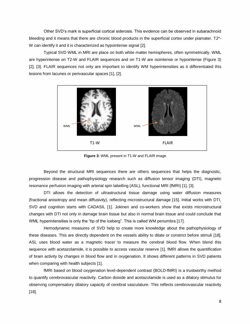
Typical SVD WML in MRI are place on both white matter hemispheres, often symmetrically. WML

are hyperintense on T2-W and FLAIR sequences and on T1-W are isointense or hypointense (Figure 3)

[2], [3]. FLAIR sequences not only are important to identify WM hyperintensities as it differentiated this

lesions from lacunes or perivascular spaces [1], [2].

Figure 3: WML present in T1-W and FLAIR image

Beyond the structural MRI sequences there are others sequences that helps the diagnostic,

progression disease and pathophysiology research such as diffusion tensor imaging (DTI), magnetic

resonance perfusion imaging with arterial spin labelling (ASL), functional MRI (fMRI) [1], [3].

DTI allows the detection of ultrastructural tissue damage using water diffusion measures

(fractional anisotropy and mean diffusivity), reflecting microstructural damage [15]. Initial works with DTI,

SVD and cognition starts with CADASIL [1]. Jokinen and co-workers show that exists microstructural

changes with DTI not only in damage brain tissue but also in normal brain tissue and could conclude that

WML hyperintensities is only the “tip of the iceberg”. This is called WM penumbra [17].

Hemodynamic measures of SVD help to create more knowledge about the pathophysiology of

these diseases. This are directly dependent on the vessels ability to dilate or constrict before stimuli [18].

ASL uses blood water as a magnetic tracer to measure the cerebral blood flow. When blend this

sequence with acetazolamide, it is possible to access vascular reserve [1]. fMRI allows the quantification

of brain activity by changes in blood flow and in oxygenation. It shows different patterns in SVD patients

when comparing with health subjects [1].

fMRI based on blood oxygenation level-dependent contrast (BOLD-fMRI) is a trustworthy method

to quantify cerebrovascular reactivity. Carbon dioxide and acetazolamide is used as a dilatory stimulus for

observing compensatory dilatory capacity of cerebral vasculature. This reflects cerebrovascular reactivity

[18].

T1-W FLAIR

WML WML

9

It is widely accepted that MRI is the most relevant tool for monitoring cerebral CADASIL. SVD MRI

changes usually precede other symptoms 10 to 15 years and normally appear at a mean age of 30 years

[6], [7]. The alterations in WM is observed on T1-W and T2-W MRI sequences in 50% of descendent

subjects that confirmed the autossomic dominant transmission [7].

As other SVD, it presents WM abnormalities in cerebral MRI [9]. All the symptomatic CADASIL

patients and some asymptomatic CADASIL patients have WM abnormalities [10].

The lesions are generally located within periventricular WM, basal ganglia, thalamus, internal

capsule and the pons [9]. Lesions can also appear in brainstem and corpus callosum [6]. Also it presents

T2-W hypersignal that is predominant in periventricular regions and in semi-ovals centers. The lesions

scores tend to increase with age [7].

Diffusion tensor do not have diagnostic value but can be important to define the clinical

importance of the lesions. It has founded to T2-W hyperintensities an increase of the mean diffusivity in

60% [4], [18].

Nowadays, new development on hardware may be have an important role in SVD. One example

is the possibility of microinfarcts study with 7 Tesla MRI [1].

1.3. Lesion segmentation

Segmentation is the classification of a pixel from an image into different groups with the same

features such as intensity or texture [19], so, pixel information is fundamental for this process [20].

Segmentation of MRI brain imaging is a very important issue for some clinical practice situations. It can be

applied in different areas such as surgical planning, surgery navigation, multimodality image registration,

lesions quantification, functional mapping, separating into different cerebral regions CSF, WM,GM), etc

[19], [21]. All over the years experts try to choose the best segmentation methodology for these

applications without success.

Segmentation methodology can be classify based on human intervention: manual segmentation,

semi-automatic segmentation and automatic segmentation [22]. In manual segmentation method the

image is labelled slice-by-slice and segmented by hand. This procedure can be influentiated by artifacts

and image quality. The disadvantages of this method is accuracy, reproducibility errors and time

consuming. So, ideally semi-automatic or automatic methods should be preferred [19]. Manual

segmentation is used nowadays for defining the “ground truth” and it is important on automated

segmentation methods evaluation. It is also used to brain atlas formation [23]. Manual segmentation is not

the only that can be influenced by image quality or images from different sources (different modalities,

sequences, etc). Semi-automatic and automatic segmentation can suffer changes in their performance too

[20].

The research to solve the segmentation problem was promote the creation and improvement of

several algorithms such as: intensity-based, thresholding, region growing, edge detection, classifiers,

10

clustering, statistical models, artificial neural networks, deformable models and atlas-guided approaches.

Some authors, in the attempt to obtain more accurate segmentation results, conjugate different methods

[19].

1.3.1. Lesion segmentation in SVD

In the last years lesions segmentation in MRI had been a challenge that a lot of researchers try,

without success, to solve. There is currently no automatic method that can be generalized for brain MRI

segmentation. Different methods were used as the reported in the topic before, and sometimes

combination methods are also employed. Here will be presented some of the research works that address

the lesions MRI segmentation issue. Some of the papers are not focus only in SVD, however pathologic

lesions presented are similar and some strategy of these methods could be important for apply in SVD in

future.

Freire et al (2016) used an iterative method based on Student’s mixture models and a probabilistic

anatomical atlas for automatic segmentation of multiple sclerosis lesions on MRI FLAIR. This approach

tries to avoid misclassification of the voxels outside the WM tissue but with similar intensities to lesion

voxels. An algorithm limitation is found in image registration because this process sometimes is not

perfect. When some lesions are in places with a bad aligned, the segmentation not have a good

performance. However this limitation could be seen as a strength because it eliminates the lesions outside

WM. Other problem found by the authors was misclassification when voxel has a significant intensity

variability [25].

Other interesting work was proposed by Noureddine et al (2015) that develop a Matlab® algorithm

to extract injured area in MRI images for segmented stroke lesions. This algorithm is based on

morphological imaging processing and region-based segmentation (region growing). The results

presented was good, especially because the authors do not used multiple MRI sequences. Therefore, the

process needs some refinements to increase sensitivity [26]

Admiraal-Behloul et al (2005) present an automatic quantification method for lesions that have

population subjects from PROSPER project (Prospective Study of Pravastatin in the Elderly at Risk). The

authors used prior maps of Montreal Neurological Institute (MNI) that need to registration to the input

images. After the registration process a FCM algorithm was applied. It was concluded that the method are

reproducibility and is robust for differences in FLAIR image slice thickness. It had also a good

performance in images with variable lesion load. However quality control by visual inspection is important

[27].

With the objective to apply wavelet functions in segmentation image Karthik et al (2016) propose a

method for discriminated lesions from normal brain tissue. Between the wavelet functions applied,

11

daubechies and de-meyer present higher differentiation in the discrimination healthy tissue from

pathologic tissue [28].

Javadpour et al. (2016) create an algorithm based on genetic and regional growth. The authors

combing neural networks with fuzzy inference systems for create a perfect nonlinear estimator that they

call neural-fuzzy network. The seeds from the growth approach will be selected automatically. This

method not necessary specify some parameters that can interferated with noise and can detects artifacts

effects. However, artifact signal could be recorded along the original signal. The authors used the SPM

boptimisedQ voxel–based morphometry (VBM). This program needs the registration of images input with

tissue probility maps, that will be represent the prior probability of each location [29].

K-NN was used by Anbeek et al (2004). The authors used a multiple spectral approach (T1-W, IR,

PD, T2-W, FLAIR) and concluded that this technique has a high sensitivity and specificity by ROC curves.

With this method the authors create a probability maps that could be an advantage factor because it is

possible to obtain different binary segmentations and segmentations with a better concordance with

reference can be obtain. This method has better results for patients with large lesion load [30].

Multispectral MRI data were used also by Jokinen et al (2015). They applied a discriminative

clustering for reduce the use of prior information. It can estimate for each voxel tissue probabilities and

characterized the WML evolution in small, intermediate or high proportion of WML. Small probabilities

usually do not enter like lesions in other method therefore can be a symbol of early WML [17].

Chyzhyk et al (2015), for automatic segmentation of stroke lesion, used a predictive capacity of

Random Forests trained associated with an Active Learning. This active learning applies a labeled training

set for build a map of data features and, this way, generated classes. The Randomm Forest classifier

predict the class of each voxel independently and classifies as lesion or no lesion. Accuracy, sensitivity

and specificity have good results for clinical applications, even if few iterations needed[31].

Lee et al (2009) proposed a power transformation method that adjusted to a non Gaussianity

tissue intensity distributions. With this methodology the author try to eliminated partial volume effect. The

big advantage is being computationally simple [32].

Si and Bhattacharjee (2016) develop an algorithm for detect MRI brain lesions without tissues

classification. For solve this problem the authors created a classifier which uses a Multi-Layer Perceptron

neural network that is trained by Levenberg-Marquardt method. Thereby, it is extracted a set of statistical

features from images and this set is used for created the ground truths in the targets images. After the

training, the algorithm classify the voxel in lesions or no lesions. The method present a good results in

specificity, accuracy and dice coefficient. However authors think that better results could be obtain

associated the method to wavelet features [33].

Lesion Identification with Neighborhood Data Analysis (LINDA) was proposed by Pustina et al

(2016). It is a supervised algorithm segmentation that uses information from each voxel and their

neighborhood and promoted hierarchical improvements of lesion estimation [34].

The authors only applied one image modality (T1-W) for analyzed chronic stroke lesions and they

employ a Random Forests approach which leads a good accuracy results. This algorithm shows high

12

sensitive rates from all real brain lesions and can predict areas of subtle intensity changes like a lesion.

Other algorithm advantage is the generation of a graded posterior probability maps that shows the

uncertainty of the model [34].

Zangeneh and Yazdi (2016) proposed a genetic algorithm based on constrain Gaussian mixture

model to segmentation lesions. In the model application the author estimated parameters take in account

some lesions constraints with the objective of incorporated prior information into Gaussian mixture model.

The application of genetic algorithm in this process allows solve nonlinear constrained problems of the

Gaussian mixture model. Gaussian mixture model by itself shows poor performance however the lesions

recognition is more accurate when there are the conjugation of Gaussian mixture with genetic algorithm

[24].

Geometric model was applied by Strumia et al (2016) to lesions segmentation without appeal

atlas registration. They used a topological priors such as the connectivity of GM and apply the Gaussian

mixture models for tissue appearance. A geometric model limitation is some non-corrections in anatomy

and regions that belong to ventricles are no suppress [35].

De et al (2016) had develop, in previous works, an adaptive vector quantization method that has

an excellent performance. These method uses self-organizing maps and vector quantization. In the most

recent research they develop parallel algorithms for use in vector quantization method. The results show

that with the parallel algorithm, computated efficiency improve without changing segmentation

performance [36].

FMRIB's Automated Segmentation Tool (FAST) uses a hidden Markov Random Field model

(HMRF) propose by Zhang et al (2001). The authors uses MRF that do not observe directly the generation

of stochastic process that it produces but can determinate the process from the field observations. Also to

estimate model parameters it was applied EM algorithm. The two approaches together improve the

accuracy and robustness of the algorithm segmentation. Because of different intensities contrast in brain

MRI image some results may not be perfect but in the most of cases analyzed results are stable. Also, this

algorithm seems to be influenced by bias field and is slow algorithm. The framework where this method is

implemented, is able to incorporate other techniques for improve segmentation results [37].

1.4. Goals and outline

WML segmentation in SVD can be time-consuming and can produce inaccurate results. In the last

years more accurate results are searched by using automatic or semi-automatic techniques; however it is

an unsolved problem because there is no optimal method for all pathologies. Nowadays, there is no

recommended method for this issue and new algorithms still be proposed. On the other hand, there are

free tools that can be used for image segmentation, but there are no specific guidelines for their utilization

in WML and SVD.

13

The main aim of this study is to create a WML segmentation pipeline, to be applied to SVD, based on

pre-existing and freely available segmentation algorithms. To accomplish this main object, the following

specific objectives were defined:

• Skull stripping optimization

• Achieved optimal results for inter and intra subjects registration

• Achieved optimal results in tissue segmentation

• Produce an accurate gold standard

The remaining of this dissertation is organized as follows: Chapter 2 presents all the data and

methodology applied to achieve the aim of this study. This also presents the statistical approach used for

results analysis. In Chapter 3 results from the analyze data will be presented. In Chapter 4 the results

obtained will be compared with others and advantages/limitations will be presented for results

improvement in future works. In Chapter 5 future directions will be introduced and conclusions of the study

will be taken.

14

Chapter 2 – Methodology

2.1. Study Population

From January 2015 to January 2016, brain MRI images were acquired at Hospital da Luz, Lisboa,

in the scope of the Neurophysim project, following appropriate inclusion criteria (defined by the

neuroradiologists associated to this project) and upon informed consent from all participants, according to

the approval by the local Ethical Committee.

The study population analyzed in this thesis is composed by sixteen subjects, between 36 and 81

years old (mean 52 ± 11 years old) including 5 men and 11 women. All the subjects have a diagnosis of

SVD, four of them with the subtype CADASIL.

2.2. Acquisition Protocol

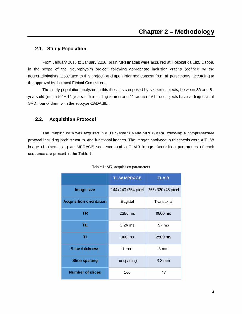
The imaging data was acquired in a 3T Siemens Verio MRI system, following a comprehensive

protocol including both structural and functional images. The images analyzed in this thesis were a T1-W

image obtained using an MPRAGE sequence and a FLAIR image. Acquisition parameters of each

sequence are present in the Table 1.

Table 1: MRI acquisition parameters

T1-W MPRAGE FLAIR

Image size 144x240x254 pixel 256x320x45 pixel

Acquisition orientation Sagittal Transaxial

TR 2250 ms 8500 ms

TE 2.26 ms 97 ms

TI 900 ms 2500 ms

Slice thickness 1 mm 3 mm

Slice spacing no spacing 3.3 mm

Number of slices 160 47

15

2.3. Image Processing

The following processing steps were performed for lesion segmentation, including: pre-processing

by skull stripping and brain extraction; co-registration of MPRAGE and FLAIR images, and normalization

to MNI space; tissue segmentation in three classes (WM, GM and CSF); and finally WML segmentation.

The FSL (FMRIB Software Library v5.0) software package was used for all the steps of image processing.

2.3.1. Pre-processing: skull stripping

Skull stripping and brain extraction is an important step for efficient registration and segmentation.

For this purpose, we used the Brain Extraction Tool (BET) from FSL software [38].

In some images BET did not yield good results in skull striping, so we performed manual brain

extraction. This requires drawing a region of interest (ROI) around the brain in all slices and removing the

information outside of the brain.

2.3.2. Image registration

For multispectral segmentation, co-registration of the multiple input images is required. We

chose to co-register the MPRAGE image to the FLAIR image space, because SVD lesions are located in

WM and they are best visualized in FLAIR images.

For our proposed segmentation process it is necessary to perform, not only this intra-subject

image co-registration (T1-W and FLAIR), but also image normalization, i.e., co-registration with a standard

image or brain template. We chose to co-register each subject’s MPRAGE image with the brain template

from the Montreal Neurologic Institute (MNI-152)).

All registration operations were performed using FMRIB’s Linear Image Registration Tool

(FLIRT). This algorithm uses a cost function for quantify the quality of registration to find the

transformation that gives less cost and interpolations to evaluate the intensity at intermediate locations

[39].

Firstly we register FLAIR in T1-W space by linear transformation using FLIRT. For cost function

corratio is used. For interpolation we use a trilinear function. The angles chosen for the first optimization

step are -90º and +90º for both x and z directions. We tested both 6 and 12 degrees of freedom (DOF).

For the registration of the MPRAGE image with the MNI image, we first employ a linear

registration step using FLIRT, with 12 DOF, and otherwise identical options to the previous registration.

Subsequently, a non-linear registration step is also employed using FMRIB’s nonlinear image registration

16

tool (FNIRT) [40]. A warp is obtained from the FNIRT process. This warp is applied for T1-W creation in

MNI space.

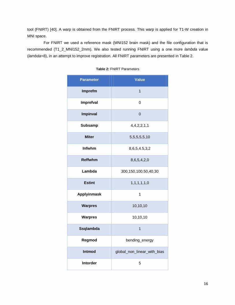
For FNIRT we used a reference mask (MNI152 brain mask) and the file configuration that is

recommended (T1_2_MNI152_2mm). We also tested running FNIRT using a one more lambda value

(lambda=8), in an attempt to improve registration. All FNIRT parameters are presented in Table 2.

Table 2: FNIRT Parameters

Parameter Value

Imprefm 1

Imprefval 0

Impinval 0

Subsamp 4,4,2,2,1,1

Miter 5,5,5,5,5,10

Infwhm 8,6,5,4.5,3,2

Reffwhm 8,6,5,4,2,0

Lambda 300,150,100,50,40,30

Estint 1,1,1,1,1,0

Applyinmask 1

Warpres 10,10,10

Warpres 10,10,10

Ssqlambda 1

Regmod bending_energy

Intmod global_non_linear_with_bias

Intorder 5

17

Biasres 50,50,50

Biaslambda 10000

Refderiv 0

The non-linear warp is inverted, so that it can be applied from MNI to MPRAGE spaces. The

linear transformations between MNI and MPRAGE and between MPRAGE and FLAIR spaces are

concatenated, and subsequently inverted. With these inverted transformation and warp, we are able to

register any image in the MNI standard space into the FLAIR space of each subject (as described in the

subsequent sections).

The segmentation of the MNI template brain image is performed using default options, into GM,

WM and CSF. Because this image corresponds to the standard template brain, it does not present any

WMLs.

2.3.3. Tissue segmentation

Tissue segmentation is performed, based on the patient’s individual images as well as on the MNI

template brain image, using FLS’s tool FAST[41].

For the segmentation of the patient’s individual images, we tested two methodologies: a

multispectral, or multichannel, modality (using both T1-W and FLAIR images) and a one-channel modality

using either T1-W or FLAIR images. It each case, we also tested three or four classification classes.

Initially, we attempted to achieve the automatic separation of WMLs from the three normal tissues,

GM, WM and CSF, by using four classes instead of three, and providing both the FLAIR as well as the

MPRAGE images as input to the multispectral segmentation algorithm. However, this approach was not

successful. In fact, WMLs were systematically classified as GM or CSF, even when four classes were

segmented. Alternatively, we attempted a different approach to obtain a WML segmentation, which

involved the comparison of the patient’s WM mask with that of a template brain, without WMLs.

The segmentation of the MNI template brain image is performed using default options, into GM,

WM and CSF. Because this image corresponds to the standard, template brain, it does not present any

WMLs.

18

2.3.4. Lesion segmentation

To obtain a segmentation of the WMLs, we subtract the WM mask obtained by multichannel

segmentation of T1-W and FLAIR into three classes from the WM mask obtained from the MNI standard

image.

In order to eliminate residual errors of this subtraction in superficial cortical regions, we apply the

BET tool to the WML mask, using an appropriate fractional intensity threshold of 0,8, 0,9 or 1.

2.4. Performance Evaluation

To evaluate the quality of the WML segmentation, we perform a qualitative and a quantitative

analysis. For qualitative measures we observe all the segmented images.

For quantitative evaluation true positive (TP), false positive (FP), true negative (TN) and false

negative (FN) are calculated and we used the following outcome measures, by comparison with a ground

truth, obtained by manual segmentation of WMLs (using the same intensity range in all the cases, 0-

1100):

The Dice coefficient (DC) is calculated by [42], [43]:

DC =2 × (GT ∩ Seg)

GS + Seg

where GT is a ground truth segmentation and Seg is an automated segmentation.

The sensitivity is calculated by [44]:

Sensitivi𝑡y =TP

TP + FN

The specificity is calculated by [44]:

Specificity =TN

TN + FP

The accuracy is calculated by [45]:

Accuracy =TP + TN

TP + FP

19

The percentage of lesion volume that is not detected is calculated by:

% Lesion volume non detected = GT − TP

GT× 100

The volume of the lesion that it is not detected is calculated by:

Lesion volume non detected =GT volume × % Lesion volume non detected

100 (𝑐𝑚3)

A one-way analysis of variance (ANOVA) was performed with factor segmentation method, for

all the performance measures (sensitivity, specificity, accuracy, DC and lesions volume non detected) in

order to test if the results were statistically significantly different. The confidence interval was 95%.

20

Chapter 3 – Results

3.

The methodology implemented has the objective to achieve the optimal result in each step. Bad

results in one step can promote lesion segmentation without quality. The data have a qualitative and

quantitative analysis. In the follow topics each step will be analyzed.

3.1. Pre-processing: skull stripping

Skull stripping was applied to all brain MRI images. More accurate results were obtained changing

the center of gravity of the initial mesh surface in each image. This center should be located between and

slightly above ventricles. Better results were achieved with FLAIR images.

Manual segmentation was required in 6 T1-W and in 3 FLAIR images because BET performance

was not efficient, especially in frontal region and cerebellum.

A B

FLAIR whitout BET

application

FLAIR after BET

application

Figure 4: Skull stripping. Comparative image before and after FLAIR application. In A it was observed a region that do not belong to brain tissue (arrow). In B the BET tool do not contemplate some brain tissue (arrow).

21

3.2. Image registration

Intra-subject registration results with different DOF in FLIRT do not change significantly and has

good correlation between FLAIR and T1-W structures (Figure 5). However inter-subject registration results

differ between using FLIRT or FNIRT (Figure 6). With FLIRT it is observed that the tissue correlation close

to ventricles has some problems that do not appear in FNIRT registration. Despite better registration

results, FNIRT registration bring us another problem. Both FNIRT registrations classify lesions areas as

GM instead of classifying as WM (Figure 6). Figure 6 (H) shows a different WM registration with different

FNIRT parameters. The registration is not optimal, however, adding a lambda=8 there are some

improvements.

Figure 5: Registration results. Comparison between FLIRT registrations. A – FLAIR; B - WM from T1-W to FLAIR

registration with FLIRT and DOF 6 ; C - WM from T1-W to FLAIR registration with FLIRT and DOF 12; D –

Overlap of WM from FLIRT DOF 12 and FLIRT DOF 6

A B C

D

WM from T1-W to FLAIR

registration with FLIRT and dof 6

WM from T1-W to FLAIR

registration with FLIRT and dof 12

22

E F

G H

WM from T1-W to FLAIR registration with FLIRT DOF 12

WM from MNI to FLAIR registration with FLIRT DOF 12

WM from MNI to FLAIR registration with FNIRT

WM from MNI to FLAIR registration with FNIRT with

lambda=8

3

2

1

3

2

2

3

1

2

1 – Overlap of WM’s

2 – WM from T1-W to FLAIR registration

3 – WM from the registration that is analyses in each image

A B C D

Figure 6: Registration results. Comparison between the WM from different registrations. A - WM from T1-W to

FLAIR registration with FLIRT DOF12; D - WM from MNI to FLAIR registration with FLIRT DOF 12; C - WM

from MNI to FLAIR registration with FNIRT ; D - WM from MNI to FLAIR registration with FNIRT with lambda=8;

E – Comparison between WM T1-W to FLAIR registration and WM MNI to FLAIR registration with FLIRT DOF

12; F – Comparison between WM T1-W to FLAIR registration and WM MNI to FLAIR registration with FNIRT;

G – Comparison between WM T1-W to FLAIR registration and WM MNI to FLAIR registration with FNIRT

lambda=8; H - Comparison between WM MNI to FLAIR registration to FNIRT and WM MNI to FLAIR

registration with FNIRT lambda=8.

23

3.3. Tissue segmentation

Different tissue segmentation was proposed. Firstly we used mono-channel segmentation (FLAIR)

in three and four classes. For three classes we can separate WM in almost all cases. In few cases we are

not able to distinguish WM from GM. Lesions are classified as GM in the majority of the cases and

sometimes in CSF. When we applied a four classes the separation of tissues is not distinct.

When we employed a multi-channel strategy (T1-W and FLAIR) the results seems to be more

accurate. In three classes, we are able to separate WM in all cases. WML are also classified as GM in all

cases and sometimes as CSF. However, when we employed a four classes classification the results do

not improve. An example of the segmentation is shown in Figure 7.

3.4. Lesion segmentation

Lesion segmentation is based on multi-channel approach with three classes and is the result of

the subtraction of the WM from MNI and the WM from multi-channel data (FLAIR and T1-W). Qualitatively,

in most cases, lesions close to ventricles are not classified as lesions. Moreover some GM tissue was

classified as lesion. These are two sources of lesions identification error that were found.

A

B C D E

Figure 7: Segmentation Results: A – FLAIR image; B –FLAIR segmentation in 3 classes; C - FLAIR

segmentation in 4 classes; D – FLAIR and T1-W segmentation in 3 classes; C – FLAIR and T1-W

segmentation in 4 classes

24

The subjects with a low WML load had more GM classified as lesion than true lesions. When we

apply BET with a fractional intensity threshold some of the GM tissue disappear. This phenomenon is

bigger with a high threshold value, however with high threshold some lesions are nullified. Figure 8

represent this analysis.

The quantitative results support the qualitative evaluation. Higher sensitivity values were found

when we do not apply BET (FNIRT standard with a mean of 48,89 % ±11,49 % and FNIRT lambda=8

FLAIR Ground Truth

Without BET BET f=0,8 BET f=0.9 BET f=1

Without BET BET f=0,8 BET f=0.9 BET f=1

Figure 8: WML segmentation results obtained by different methods

25

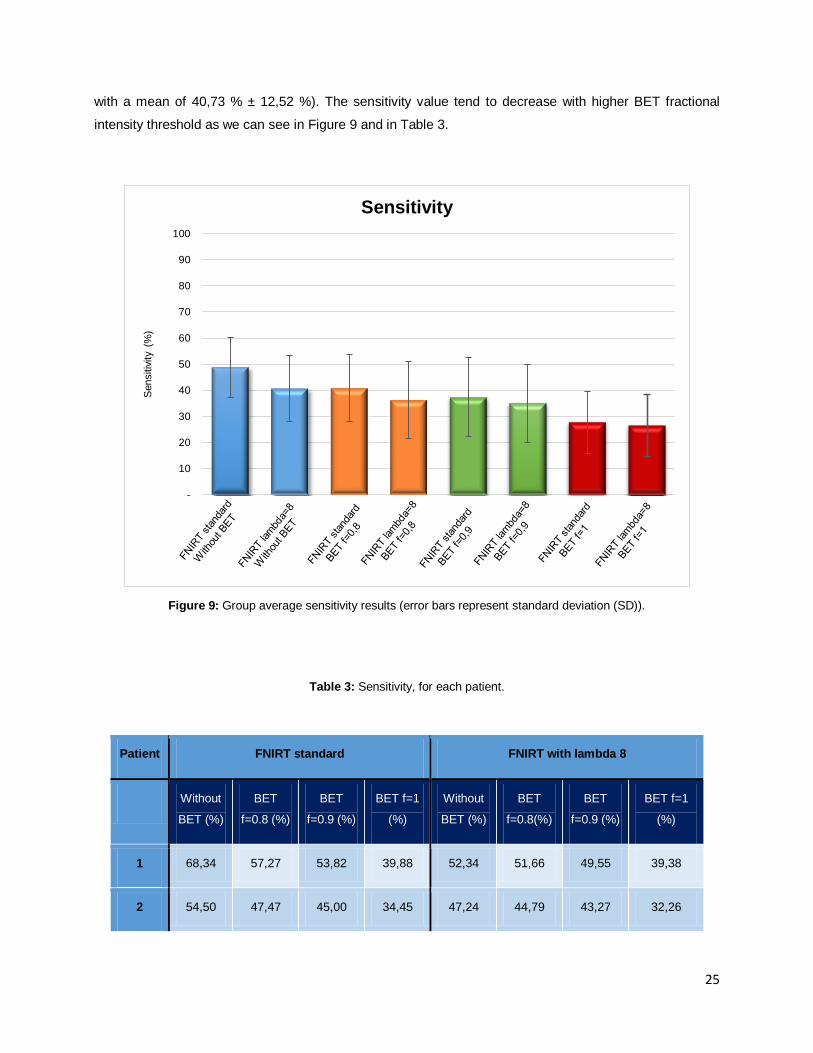
with a mean of 40,73 % ± 12,52 %). The sensitivity value tend to decrease with higher BET fractional

intensity threshold as we can see in Figure 9 and in Table 3.

Figure 9: Group average sensitivity results (error bars represent standard deviation (SD)).

Table 3: Sensitivity, for each patient.

Patient FNIRT standard FNIRT with lambda 8

Without

BET (%)

BET

f=0.8 (%)

BET

f=0.9 (%)

BET f=1

(%)

Without

BET (%)

BET

f=0.8(%)

BET

f=0.9 (%)

BET f=1

(%)

1 68,34 57,27 53,82 39,88 52,34 51,66 49,55 39,38

2 54,50 47,47 45,00 34,45 47,24 44,79 43,27 32,26

-

10

20

30

40

50

60

70

80

90

100

Sensitiv

ity (

%)

…

Sensitivity

26

3 51,26 55,82 56,08 38,26 54,89 52,23 51,92 35,98

4 62,38 59,12 57,33 41,42 60,51 56,12 54,20 40,81

5 55,33 42,39 38,68 25,73 42,92 40,77 38,83 27,55

6 45,02 43,40 40,04 30,70 44,86 41,45 39,53 30,39

7 46,73 38,91 36,95 34,95 38,77 34,99 34,53 32,56

8 40,44 29,33 25,72 24,76 27,71 22,95 22,87 22,16

9 33,13 23,04 18,12 9,94 25,46 19,84 17,56 10,09

10 56,60 48,64 46,06 25,45 48,52 44,44 43,16 22,30

11 55,71 55,26 54,97 45,80 55,81 53,63 53,65 44,20

12 58,13 42,11 39,29 31,49 39,99 35,62 35,19 28,13

13 30,95 23,87 14,02 9,63 23,59 13,46 9,79 6,69

14 54,06 40,86 39,13 27,33 41,37 38,86 38,64 30,63

15 40,66 24,04 17,40 15,33 23,20 14,59 13,80 12,21

16 29,04 22,37 14,82 8,82 24,48 16,24 14,51 9,38

MEAN 48,89 40,87 37,34 27,75 40,73 36,35 35,06 26,54

SD 11,49 12,95 15,14 11,74 12,52 14,65 14,95 11,76

Specificity results and accuracy results have the inverse behavior when comparing with

sensitivity. So, FNIRT with BET and high a fractional intensity threshold present better results. Also the

results are generally higher with FNIRT lambda=8 as observed in Table 4, in Table 5, in Figure 10 and in

Figure 11. For specificity and accuracy the higher value belongs to FNIRT lambda=8 (98,92% ± 0,26%

and 97,08 %±1,71% respectively).

27

Figure 10: Group average specificity results (error bars represent SD).

Table 4: Specificity for each patient.

Patient FNIRT standard FNIRT with lambda 8

Without

BET (%)

BET

f=0.8 (%)

BET

f=0.9 (%)

BET

f=1 (%)

Without

BET (%)

BET

f=0.8(%)

BET

f=0.9 (%)

BET f=1

(%)

1 85,54 95,88 97,32 98,62 95,20 96,31 97,55 98,71

2 84,62 95,61 97,02 98,69 94,93 96,56 97,73 99,07

3 84,11 95,92 97,15 98,85 95,30 96,68 97,76 99,09

-

10

20

30

40

50

60

70

80

90

100

Specific

ity

(%)

Specificity

28

4 83,95 95,67 96,91 98,59 96,11 96,96 97,69 98,88

5 85,11 97,25 98,06 99,08 95,67 97,28 98,07 99,06

6 86,49 96,43 97,74 99,15 95,72 97,43 98,40 99,29

7 82,74 96,47 97,59 98,74 94,96 96,69 97,91 98,94

8 84,11 95,89 96,77 98,44 95,51 96,68 97,46 98,56

9 84,34 94,40 96,74 98,68 93,94 95,41 97,26 98,91

10 84,07 94,91 96,62 98,48 94,04 96,62 97,77 98,90

11 85,94 96,38 97,33 98,72 95,71 97,09 97,97 98,99

12 85,35 96,79 97,24 98,48 95,99 97,34 97,73 98,67

13 84,41 96,63 97,43 98,94 96,23 96,54 97,67 99,03

14 83,05 96,96 97,39 98,46 95,46 96,14 97,21 98,28

15 85,53 96,63 97,88 99,07 95,61 97,44 98,43 99,22

16 83,47 95,59 97,51 99,07 94,94 96,22 97,81 99,15

MEAN 84,55 96,09 97,29 98,75 95,33 96,71 97,78 98,92

SD 1,04 0,76 0,41 0,25 0,66 0,55 0,34 0,26

29

Figure 11: Group average accuracy results (error bars represent SD).

Table 5: Accuracy for each patient.

Patient FNIRT standard FNIRT with lambda 8

Without

BET (%)

BET

f=0.8 (%)

BET

f=0.9 (%)

BET

f=1 (%)

Without

BET (%)

BET

f=0.8(%)

BET

f=0.9 (%)

BET f=1

(%)

1 84,65 93,90 95,16 95,70 93,07 94,09 95,17 95,77

2 84,05 94,70 96,06 97,50 94,03 95,60 96,73 97,84

3 83,63 95,39 96,65 98,09 94,76 96,11 97,18 98,28

4 83,36 94,67 95,88 97,08 95,17 95,88 96,53 97,34

-

10

20

30

40

50

60

70

80

90

100A

ccura

cy (

%)

…

Accuracy

30

5 84,65 96,40 97,20 98,01 94,89 96,45 97,20 98,01

6 85,94 95,72 97,02 98,29 95,04 96,72 97,65 98,41

7 81,08 93,81 94,93 95,90 92,37 93,93 95,08 95,98

8 81,73 92,19 93,05 94,55 91,70 92,78 93,51 94,52

9 83,97 93,91 96,24 98,10 93,46 94,91 96,73 98,32

10 83,98 94,76 96,46 98,25 93,89 96,46 97,60 98,66

11 85,34 95,57 96,53 97,72 94,93 96,25 97,12 97,94

12 84,76 95,57 96,01 97,06 94,75 96,02 96,39 97,17

13 80,40 91,10 91,65 92,74 90,51 90,75 91,55 92,59

14 81,96 94,84 95,31 95,90 93,42 94,06 95,08 95,82

15 85,20 96,06 97,33 98,48 95,05 96,85 97,82 98,60

16 82,71 94,55 96,43 97,89 93,93 95,17 96,71 97,97

MEAN 83,59 94,57 95,74 96,95 93,81 95,13 96,13 97,08

SD 1,61 1,39 1,51 1,60 1,35 1,66 1,69 1,71

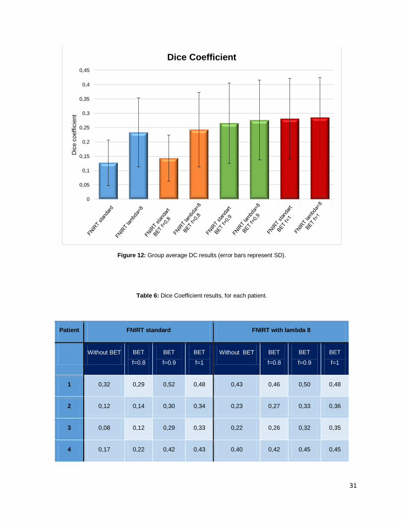
DC results follow the same trend of specificity and accuracy results. Also it is observed that there

is a high difference between the two FNIRT registrations without BET. FNIRT with lambda=8 has a DC

value double than FNIRT standard (0,23±0,12 and 0,13±0,08 respectively). However we are able to

increase this value with the BET application, higher the fractional intensity threshold, higher is DC. The

DC results are present in Figure 12 and Table 6.

31

Figure 12: Group average DC results (error bars represent SD).

Table 6: Dice Coefficient results, for each patient.

Patient FNIRT standard FNIRT with lambda 8

Without BET BET

f=0.8

BET

f=0.9

BET

f=1

Without BET BET

f=0.8

BET

f=0.9

BET

f=1

1 0,32 0,29 0,52 0,48 0,43 0,46 0,50 0,48

2 0,12 0,14 0,30 0,34 0,23 0,27 0,33 0,36

3 0,08 0,12 0,29 0,33 0,22 0,26 0,32 0,35

4 0,17 0,22 0,42 0,43 0,40 0,42 0,45 0,45

0

0,05

0,1

0,15

0,2

0,25

0,3

0,35

0,4

0,45D

ice c

oeff

icie

nt

Dice Coefficient

32

5 0,10 0,12 0,28 0,27 0,20 0,25 0,29 0,29

6 0,08 0,10 0,25 0,31 0,20 0,24 0,30 0,33

7 0,19 0,24 0,39 0,43 0,32 0,34 0,39 0,42

8 0,20 0,19 0,28 0,32 0,28 0,25 0,27 0,30

9 0,03 0,03 0,06 0,06 0,05 0,05 0,07 0,07

10 0,02 0,02 0,07 0,08 0,05 0,07 0,10 0,09

11 0,13 0,16 0,37 0,43 0,30 0,35 0,42 0,45

12 0,14 0,16 0,29 0,31 0,26 0,28 0,29 0,30

13 0,20 0,19 0,19 0,16 0,30 0,17 0,14 0,11

14 0,18 0,23 0,37 0,32 0,33 0,32 0,36 0,35

15 0,04 0,04 0,08 0,12 0,07 0,06 0,08 0,11

16 0,04 0,06 0,10 0,10 0,11 0,08 0,10 0,11

MEAN 0,13 0,14 0,27 0,28 0,23 0,24 0,28 0,29

SD 0,08 0,08 0,14 0,14 0,12 0,13 0,14 0,14

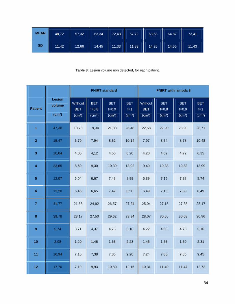
We also analyzed the lesion identification error. The behavior of this evaluated parameter is

similar to sensitivity. So with higher BET fractional intensity threshold parameter higher is the lesion

volume lesion that it is not identified. However all the values are high, with BET fractional intensity

threshold parameter of 1, the percentage of not identified lesions are higher than 70%. The results can be

observed in Figure 13, Table 7 and Table 8.

33

Table 7: Lesion volume non detected (percentage), for each patient.

Patient FNIRT standard FNIRT with lambda 8

Without

BET (%)

BET

f=0.8 (%)

BET

f=0.9 (%)

BET

f=1 (%)

Without

BET (%)

BET

f=0.8(%)

BET

f=0.9 (%)

BET f=1

(%)

1 29,09 40,82 46,18 60,12 47,66 48,34 50,45 60,62

2 43,89 51,33 55,09 65,56 51,53 55,21 56,73 67,74

3 40,42 41,01 45,38 61,74 41,81 46,73 47,05 63,30

4 35,92 39,31 43,93 58,85 39,76 43,88 45,80 59,19

5 41,78 55,24 62,06 74,51 57,08 59,23 61,17 72,45

6 52,91 54,49 60,87 69,64 53,20 58,55 60,47 69,61

7 51,66 59,66 63,63 65,20 59,95 65,01 65,47 67,44

8 58,25 69,14 74,48 75,27 70,57 77,05 77,13 77,84

9 64,66 76,17 82,74 90,16 73,58 80,16 82,44 89,91

10 40,34 49,08 55,02 74,84 48,94 55,56 56,84 77,70

11 42,25 43,53 46,40 54,78 42,73 46,37 46,35 55,80

12 40,63 56,08 61,03 68,64 58,25 64,38 64,81 71,87

13 66,73 73,95 86,06 90,40 73,35 86,54 90,21 93,31

14 44,03 57,47 61,66 72,91 56,89 61,14 61,36 69,37

15 57,63 73,97 83,51 85,07 74,81 85,41 86,20 87,79

16 69,31 75,81 85,36 91,23 73,34 83,76 85,49 90,62

34

MEAN 48,72 57,32 63,34 72,43 57,72 63,58 64,87 73,41

SD 11,42 12,66 14,45 11,33 11,83 14,26 14,56 11,43

Table 8: Lesion volume non detected, for each patient.

Patient

Lesion

volume

(cm3)

FNIRT standard FNIRT with lambda 8

Without

BET

(cm3)

BET

f=0.8

(cm3)

BET

f=0.9

(cm3)

BET

f=1

(cm3)

Without

BET

(cm3)

BET

f=0.8

(cm3)

BET

f=0.9

(cm3)

BET

f=1

(cm3)

1 47,38 13,78 19,34 21,88 28,48 22,58 22,90 23,90 28,71

2 15,47 6,79 7,94 8,52 10,14 7,97 8,54 8,78 10,48

3 10,04 4,06 4,12 4,55 6,20 4,20 4,69 4,72 6,35

4 23,65 8,50 9,30 10,39 13,92 9,40 10,38 10,83 13,99

5 12,07 5,04 6,67 7,48 8,99 6,89 7,15 7,38 8,74

6 12,20 6,46 6,65 7,42 8,50 6,49 7,15 7,38 8,49

7 41,77 21,58 24,92 26,57 27,24 25,04 27,15 27,35 28,17

8 39,78 23,17 27,50 29,62 29,94 28,07 30,65 30,68 30,96

9 5,74 3,71 4,37 4,75 5,18 4,22 4,60 4,73 5,16

10 2,98 1,20 1,46 1,63 2,23 1,46 1,65 1,69 2,31

11 16,94 7,16 7,38 7,86 9,28 7,24 7,86 7,85 9,45

12 17,70 7,19 9,93 10,80 12,15 10,31 11,40 11,47 12,72

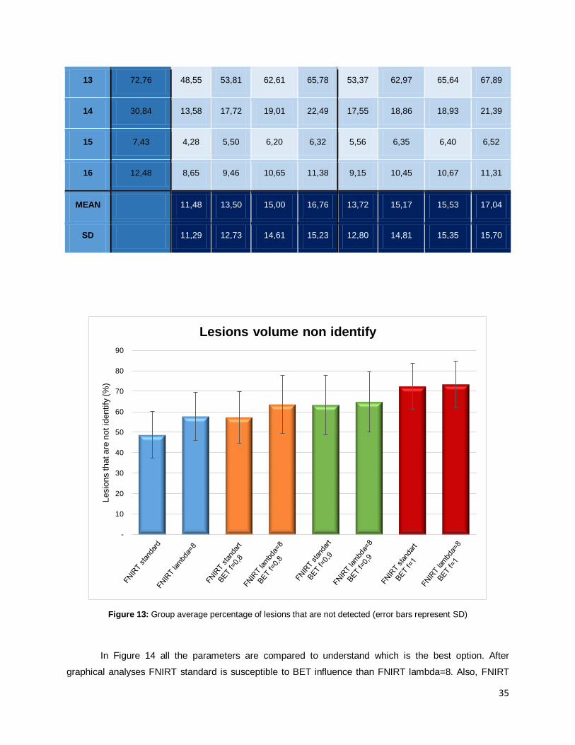
35

13 72,76 48,55 53,81 62,61 65,78 53,37 62,97 65,64 67,89

14 30,84 13,58 17,72 19,01 22,49 17,55 18,86 18,93 21,39

15 7,43 4,28 5,50 6,20 6,32 5,56 6,35 6,40 6,52

16 12,48 8,65 9,46 10,65 11,38 9,15 10,45 10,67 11,31

MEAN 11,48 13,50 15,00 16,76 13,72 15,17 15,53 17,04

SD 11,29 12,73 14,61 15,23 12,80 14,81 15,35 15,70

Figure 13: Group average percentage of lesions that are not detected (error bars represent SD)

In Figure 14 all the parameters are compared to understand which is the best option. After

graphical analyses FNIRT standard is susceptible to BET influence than FNIRT lambda=8. Also, FNIRT

-

10

20

30

40

50

60

70

80

90

Lesio

ns that are

not id

entify

(%

)

Lesions volume non identify

36

lambda=8 without BET application seems to have good results because do not have low accuracy and

specificity and presents an intermediate DC result. Sensitivity results are not reasonable comparing to

others results and the volume of lesion that is not identified by automatic segmentation is not the worst.

Figure 14: Comparison between the different performance measures for the different pipeline options tested. Grey

line divided the results obtained by using different BET in FNIRT standard and in FNIRT lambda=8.

The ANOVA showed that all performance measures improved varied significantly across

segmentation method (F=4,82; p<0.05); specificity (F=991,95; p<0.05); accuracy (F=125,90; p<0.05); DC

(F=4,18; p<0.05); lesion volume non detected (F=06,06; p<0.05).

0

10

20

30

40

50

60

70

80

90

100

FNIRTstandard

FNIRTstandart

BET f=0,8

FNIRTstandart

BET f=0,9

FNIRTstandartBET f=1

FNIRTlambda=8

FNIRTlambda=8BET f=0,8

FNIRTlambda=8BET f=0,9

FNIRTlambda=8BET f=1

Perc

enta

ge (

%)

Camparation between different results

Lesionvolume nonidentify

Sensitivity

Specificity

Accuracy

Dice

37

Chapter 4 – Discussion

This study aimed to develop a pipeline for automatic WML segmentation of MRI images from SVD

patients. All the steps in the pipeline are analyzed carefully because accurate results in each one are

required for optimized lesions segmentation.

The initial step is skull stripping. When this procedure is done manually requires a lot of time to

achieve good results, so an accurate automatic method is important. Our results about this step are not

the best because 9 of 32 images need a manual skull stripping. Popescu et al in the attempt to optimize

parameters to increase BET performance in T1-W images from multiple scleroses concluded that for

some acquisitions protocols the results are not satisfactory and the reason behind is the amount of neck

slices present in the image and spatial intensity inhomogeneity. One of the methods to achieve better

results in BET step is eliminating the neck from our images [46]. Leung et al. compared four methods of

brain extraction and concluded that this protocol tend to exclude temporal and frontal lobe as well as

cerebellum. In our study, bad BET results present the same lake in frontal lobe and cerebellum tissue.

However, comparing with other software protocols BET presents more accurate results and higher median

Jaccard [47].

In our work, registration has the objective to transport T1-W to the FLAIR space to a multichannel

segmentation with FAST. Also registration with MNI is required. We employed FLIRT for T1-W and FLAIR

registration between same individuals and the results are accurate. However, registration between MNI to

FLAIR and MNI to T1-W with FLIRT is not so positive. The reason for these results is the original data.

MNI is a standard image while FLAIR and T1-W are from different patients. Even with 12 DOF of FLIRT

for inter-subjects registration, it may be necessary other functions that can change the brain shape to

adjust the different brain structures. FNIRT registration demonstrates more accurate results than FLIRT

for these cases and seems to more perfect with the application of lambda=8. This parameter is considered

a “fudge factor” in FNIRT registration because it can balance between images similarities and smooth.

However, better results are required to increase the segmentation performance.

Best quality contrast image should be used as a reference in order to achieve accurate

registrations. In this case, MNI is a reference for its registration with the other images and T1-W is a

reference when it registers with FLAIR. If we require one image with more contrast quality in other spaces

(ex. MNI in the FLAIR space) we use the inverse transformation.

Other request for this study is that all the images should be in FLAIR space. The reason is related

with the fact that one of the MRI images characteristics for SVD is hyperintensities in WM on FLAIR

sequence. If the study was not drawn in this space, lesions alteration could be appearing and the results

will suffer a bias. So it is important to work with the data in the original space for more accurate results.

Other step analyzed was tissue segmentation. Three classification classes have better results

when compared with four classes. The main idea to use a four classes approach comes from the

38

possibility that, with a multi-channel registration, lesions appear as a fourth class. WML hyperintensities in

FLAIR can be visualized as hypointense signal in T1-W brain image.

FAST uses a MRF model. This model is characterized by mutual influences between pixel [19]. If

we conjugate the images, maybe the model could identify the hyperintensities in FLAIR in same locations

of hypointensities in T1-W and identifies as another class. However this did not happen, multi-channel

approach could separate the tissues more specifically than when we analyzed only FLAIR segmented

images.

Not always extra features are necessary and can decrease algorithm performance. It is important

to identify an optimal set of features. In this case, integrating both images reduce the uncertainty and

increase the accuracy of segmentation. Admiraal-Behoul et al also uses a multi-channel approach (PD,

T2-W and FLAIR) for the same fact. Other reason is to eliminate hyperintese artifacts from FLAIR images

[33].

In tissue segmentation results, lesions belong to GM in all cases and to GM and CSF in few

cases. One reason that can be behind this result are the intensity similarities from these tissues in FLAIR

images. Thereby, WML can appear like hyperintensities (similar to the intensity of GM on FLAIR image)

and as lacunes that have no signal as CSF [2], [3]. Thus multi-channel image with three classes was used

for SVD lesion segmentation.

We want to isolate WML. Tissue segmentation was required not only to separate WML but also to

separate WM from other classes. So, if we are not able to put WML in a single class we need to change

the approach. Thus, in patient’s WM we know that pixel where lesions are located do not belong to WM

class and if we subtract this WM with the WM of a pattern without lesions (MNI’s WM) we should obtain

the WML images. However, in our research, this is not true. One possibility for this outcome is a not

perfect registration. Almost all the lesions which have an incorrect classification are close to the ventricles

and outside brain regions (GM are incorrectly classified as a lesion). The reason for this result is a non-

optimal that leads to errors classifications in MNI and this missclassified tissue in MNI becomes FN or FP.

Besides that with big lesions FAST classifies MNI images as GM, so when we applied the subtraction

there is no WM in MNI image in the lesion location. This problem is more obvious when we use a better

registration (FNIRT with lambda=8) and can be a reason for less sensitivity in this case.

The results from this step were promising, however too many misclassifications are still present.

Pustina et al have found the same problem [34].

To brush away some misclassified lesions, we used the fractional intensity threshold from BET

parameters. The objective is to eliminate all the GM that was classify as lesion and decrease the FP rate.

The better results were achieved with a threshold of 1 even when compared with the automatic

segmentation lesions image without BET implementation. This parameter determines the location of the

final segmented edge.

This automatic segmentation, with a higher fractional intensity threshold, has high specificity

values, however the sensitivity values are not so satisfactory. The accuracy results are reasonable. The

sensitivity represents the correct lesions identification and decreases when we augment fractional

39

intensity threshold because of some nullified TP pixel. This is also the reason for the results with volume

lesion not identified. These values are lower when sensitivity results are also lower, which is an expected

result. Discrepancies of the sensitivity results between patients are high in all cases [44].

Specificity measures the ability of the method to identify non lesion pixel and the obtained results

are very satisfactory. The reason for higher values with higher fractional intensity threshold is the

elimination of GM tissue that was misclassified [44].

The accuracy represents the true positive pixel, thus with lambda=8 and fractional intensity

threshold of 1, 97,08% of pixels are correctly identified. It is the higher value obtained.

Dice coefficient is an evaluation metric propose by several authors for image segmentation [48],

[49]. It consists on the special overlap index and represents reproducibility. A reasonable DC value is

higher than 0,7 [27], [38]. Our results are very low comparing with this value (all of the DC values are less

than 0,3) and better DC results come from patients with a high WML load.

An important result is the lesion quantification that is not identified by the automatic segmentation.

The values are high and trend to increase when we apply BET. However it is not satisfactory for clinical

practice yet.

FNIRT lambda=8 without BET application seems to be the more consensual when we analyze all

the results. It does not have the best result in any evaluated parameter but when we proceed to the

comparison between all of the methods used it is the methodology that have more true results and it is

capable to identify a high lesion percentage.

When comparing the results with other studies the results are not satisfactory. Anbeek et al [43],

Si et al [33], Admiraal-Behloulet al [27], Jokinen et al[17] Pustina et al [34], Strumia et al [35] concluded

that a small WML load have worse results than with the high lesion load. So this is in agreement with our

results. However the algorithm that these authors proposed have higher DC results than ours. Table 9

shows the different DC results from papers.

Table 9: Different DC results from papers

Papers DC

Anbeek et al 0,81

Si et al 0,87

Admiraal-Behloul et al 0,75

Pustina et al 0,70

Strumia et al 0,520

One reason for low DC in a small WML load could be the small reference area and small prior

probability [43].

40

A study limitation is the gold standard. This reference image is obtained by drawing a ROI in brain

WML. This procedure should be done by an expert however this was not possible. So, we based in

literature information about SVD characterization to obtain this image. Even experts have some

discordance between them. This detail turns this work less accurate because experience in MRI brain

visualization is fundamental to achieve better results. Although, this pipeline is time consuming for some

steps.

Using a free framework is the biggest advantage, because all people can use it. There are other

free frameworks for lesions segmentation and quantification. MSMetrix is available in

https://msmetrix.icometrix.com. The big disadvantage of MSMetrix is that we only have access to the

report of lesion segmentation and we are not able to visualize all the slices. So is a blind user framework

that requires all users to believe in the result that give us.

41

Chapter 5 – Conclusion

Characterization of WM hyperintensites on FLAIR images is an important feature for diagnosis

and prognosis of SVD. There are a lot of researches involving tissue segmentation, tumor brain

segmentation, acute stroke lesions segmentation or for general lesions segmentation. However, in this

specific pathology there are only a few number of researches and no segmentation method defined.

There are two basic requirements for an image segmentation method: one is the segmentation

accuracy that is desired to be as high as possible, and the other is the processing speed that should be

fast. The images processing is done in a slow framework. Also the results are not so good. Towards these

results, changes in the methodology should be done.

For future work, we could apply vertical gradient in fractional intensity threshold when we use this

parameter to eliminate GM misclassification. This can cut off more FP pixels and preserve the TP pixels

eliminated in this procedure. Also, it could be important to investigated if WML quantification obtained in

this way may contribute a useful biomarker of SVD.

Registration of PD images with FLAIR and T1-W can improve tissue segmentation because of

FLAIR hyperintensities artifacts. The application of this registration will produce more accurate tissue

segmentation and maybe more accurate lesion segmentation.

One of the problems report is the inter-subject registration. More accurate registration outcomes

promote a better WML classification. Results from FNIRT are satisfactory but if we change some

parameters such as lambda we believe that a better WM registration is possible from the MNI and FLAIR

images. Also, a more correct WML classification is achieved.

Other possibility is using the GM tissue mask instead of WM, because the majority of

hyperintense WML belongs to GM classification and the other lesions that are not as GM are lacunes and

belongs to CSF. So if our main interest is only hyperintese WML localization, this approach should be

taken.

We think that better results are possible with this free framework. However more parameters

should be analyzed in future works and maybe a more efficient pipeline will be obtained.

42

References

[1] G. Banerjee, D. Wilson, H. R. Jäger, and D. J. Werring, “Novel imaging techniques in cerebral

small vessel diseases and vascular cognitive impairment,” Biochim. Biophys. Acta - Mol. Basis

Dis., vol. 1862, no. 5, pp. 926–938, 2016.

[2] J. M. Wardlaw, E. E. Smith, G. J. Biessels, C. Cordonnier, F. Fazekas, R. Frayne, R. I. Lindley, J.

T. O. Brien, F. Doubal, M. Duering, N. C. Fox, S. Greenberg, V. Hachinski, I. Kilimann, V. Mok, R.

Van Oostenbrugge, L. Pantoni, O. Speck, B. C. M. Stephan, S. Teipel, A. Viswanathan, D.

Werring, C. Chen, and C. Smith, “Neuroimaging standards for research into small vessel disease

and its contribution to ageing and neurodegeneration,” Lancet Neurol., vol. 12, no. 8, pp. 822–838,

2013.

[3] L. Pantoni, “Cerebral small vessel disease : from pathogenesis and clinical characteristics to

therapeutic challenges,” Lancet Neurol., vol. 9, no. 7, pp. 689–701, 2010.

[4] A. Joutel and F. M. Faraci, “Cerebral Small Vessel Disease,” Stroke, vol. 45, no. 4, pp. 1215–1221,

2014.

[5] W. R. Brown, D. M. Moody, V. R. Challa, C. R. Thore, and J. A. Anstrom, “Venous collagenosis

and arteriolar tortuosity in leukoaraiosis,” J. Neurol. Sci., vol. 203–204, pp. 159–163, 2002.

[6] H. Chabriat, A. Joutel, M. Dichgans, E. Tournier-Lasserve, and M. G. Bousser, “Cadasil,” Lancet

Neurol., vol. 8, no. 7, pp. 643–653, 2009.

[7] H. Chabriat and M. Bousser, “CADASIL (‘ cerebral autosomal dominant arteriopathy with

subcortical infarcts and leukoencephalopathy ’) Cerebral autosomal dominant arteriopathy with

subcortical infarcts and leukoencephalopathy ( CADASIL ),” EMC-Neurologie, vol. 1, no. 2, pp.

156–168, 2004.

[8] D. W. Desmond, J. T. Moroney, T. Lynch, S. Chan, S. S. Chin, and J. P. Mohr, “The Natural

History of CADASIL A Pooled Analysis of Previously Published Cases,” Stroke, vol. 30, no. 6, pp.

1230–1233, 1999.

[9] R. N. Kalaria, M. Viitanen, H. Kalimo, M. Dichgans, and T. Tabira, “The pathogenesis of CADASIL:

An update,” J. Neurol. Sci., vol. 226, no. 1–2 SPEC.ISS., pp. 35–39, 2004.

[10] M. Dichgans, M. Mayer, I. Uttner, R. Bruning, J. Muller-hocker, G. Rungger, M. Ebke, T.

Klockgether, and T. Gasser, “The Phenotypic Spectrum of CADASIL : Clinical Findings in 102

Cases,” Ann Neurol, vol. 44, no. 5, pp. 731–739, 1998.

[11] M. O’Sullivan, “Imaging small vessel disease: Lesion topography, networks, and cognitive deficits

investigated with MRI,” Stroke, vol. 41, no. 10 SUPPL. 1, pp. 154–159, 2010.

[12] T. Ai, J. N. Morelli, X. Hu, D. Hao, F. L. Goerner, B. Ager, and V. M. Runge, “A historical overview

of Magnetic Resonance Imaging, focusing on technological innovations.,” Invest. Radiol., vol. 47,

43

no. 12, pp. 725–741, 2012.

[13] M. F. Reiser, W. Semmler, and H. Hricak, Magnetic Resonance Tomography. Springer Science &

Business Media, 2007.

[14] M. Filippi, N. de Stefano, and V. Dousset, MR Imaging in White Matter Diseases of the Brain and

Spinal Cord. New York: Springer Science & Business Media, 2005.

[15] H. S. Chrysikopoulos, Clinical MR Imaging and Physics, Springer. Corfu, 2009.

[16] P. Maillard, O. Carmichael, D. Harvey, E. Fletcher, B. Reed, D. Mungas, and C. Decarli, “FLAIR

and Diffusion MRI Signals Are Independent Predictors of White Matter Hyperintensities,” Am. J.

Neuroradiol., vol. 34, pp. 54–61, 2013.

[17] H. Jokinen, N. Gonçalves, R. Vigário, J. Lipsanen, F. Fazekas, D. Inzitari, L. Pantoni, T. Erkinjuntti,

and S. Group, “Early-Stage White Matter Lesions Detected by Multispectral MRI Segmentation

Predict Progressive Cognitive Decline,” Front. Neurosci., vol. 9, no. December, pp. 1–9, 2015.

[18] M. M. A. Conijn, J. M. Hoogduin, Y. Van Der Graaf, J. Hendrikse, P. R. Luijten, and M. I. Geerlings,

“Microbleeds , lacunar infarcts , white matter lesions and cerebrovascular reactivity — A 7 T study

☆,” Neuroimage, vol. 59, no. 2, pp. 950–956, 2012.

[19] R. Xu, L. Luo, and J. Ohya, “Segmentation of Brain MRI,” in Advances in brain Imaging, V.

Chaudhary, Ed. Shangai: In Tech, 2012, pp. 143–170.

[20] M. W. Khan, “A Survey : Image Segmentation Techniques,” Int. J. Futur. Cumputer Commun., vol.

3, no. 2, pp. 89–93, 2014.

[21] J. A. Shah and S. R. Suralkar, “A Review on Brain Tumor Segmentation Techniques for MRI

Images,” in International Conference on Global Trends in Engineering, Technology and

Management (ICGTETM-2016), 2016, pp. 323–330.

[22] N. M. Zaitoun and M. J. Aqel, “Survey on Image Segmentation Techniques,” Procedia - Procedia

Comput. Sci., vol. 65, no. Iccmit, pp. 797–806, 2015.

[23] I. D. T, B. Goossens, and W. Philips, “MRI Segmentation of the Human Brain : Challenges ,

Methods , and Applications,” Comput. Math. Methods Med., vol. 2015, pp. 1–23, 2015.

[24] D. Zangeneh and M. Yazdi, “Automatic Segmentation of Multiple Sclerosis Lesions in Brain MRI

Using Constrained GMM and Genetic Algorithm,” in 2016 24th Iranian Conference on Electrical

Engineering (ICEE), 2016, pp. 832–837.

[25] P. G. L. Freire and R. J. Ferrari, “Automatic iterative segmentation of multiple sclerosis lesions

using Student ’ s t mixture models and probabilistic anatomical atlases in FLAIR images,” Comput.

Biol. Med., vol. 73, pp. 10–23, 2016.

[26] R. Noureddine, K. Tarhini, and S. Saleh, “Segmentation and Extraction of Brain Injury Lesions from

MRI Images : Matlab Implementation,” in 2015 International Conference on Advances in

Biomedical Engineering (ICABME), 2015, pp. 45–48.

[27] F. Admiraal-Behloul, D. M. J. Van Den Heuvel, H. O. M. J. P. Van Osch, J. Van der Grond, M. A.

van Buchem, and J. H. C. Reiber, “Fully automatic segmentation of white matter hyperintensities in

44

MR images of the elderly,” NeuroIma, vol. 28, no. 3, pp. 607–617, 2005.

[28] R. Karthik and R. Menaka, “Statistical characterization of ischemic stroke lesions from MRI using

discrete wavelet transformation,” ECTI Trans. Eletr. Eng. Electron. Commun., vol. 14, no. 2, pp.

57–64, 2016.

[29] A. Javadpour and A. Mohammadi, “Improving Brain Magnetic Resonance Image (MRI)

Segmentation via a Novel Algorithm based on Genetic and Regional Growth,” J. Biomed. Phys.

Eng., vol. 6, no. 2, pp. 1–14, 2016.

[30] P. Anbeek, K. L. Vincken, M. J. P. Van Osch, R. H. C. Bisschops, and J. Van Der Grond,

“Probabilistic segmentation of white matter lesions in MR imaging,” NeuroImag, vol. 21, no. 3, pp.

1037–1044, 2004.

[31] D. Chyzhyk, R. Dacosta-Aguayo, M. Mataro, and M. Graña, “An active learning approach for stroke

lesion segmentation on multimodal MRI data,” Neuroc, vol. 150, pp. 26–36, 2015.

[32] J. Lee, H. Su, P. E. Cheng, M. Liou, J. A. D. Aston, A. C. Tsai, and C. Chen, “MR Image

Segmentation Using a Power Transformation Approach,” IEEE Trans. Med. Imaging, vol. 28, no. 6,

pp. 894–905, 2009.

[33] T. Si, A. De, and A. K. Bhattacharjee, “Artificial Neural Network based Lesion Segmentation of

Brain MRI,” Commun. Appl. Electron., vol. 4, no. 5, pp. 1–5, 2016.

[34] D. Pustina, H. B. Coslett, P. E. Turkeltaub, N. Tustison, M. F. Schwartz, and B. Avants,

“Automated Segmentation of Chronic Stroke Lesions Using LINDA : Lesion Identification With

Neighborhood Data Analysis,” Hum. Brain Mapp., vol. 1421, no. 4, pp. 1405–1421, 2016.

[35] M. Strumia, F. R. Schmidt, C. Anastasopoulos, C. Granziera, G. Krueger, and T. Brox, “White

Matter MS-Lesion Segmentation Using a Geometric Brain Model,” IEEE Trans. Med. Imaging, vol.

34, no. 7, pp. 1636–1646, 2016.

[36] A. De, Y. Zhang, and C. Guo, “Neurocomputing A parallel adaptive segmentation method based on

SOM and GPU with application to MRI image processing,” Neurocomputing, vol. 198, pp. 180–189,

2016.

[37] Y. Zhang, S. Smith, and M. Brady, “Hidden Markov Random Field Model and Segmentation of

Brain MR Images,” IEEE Trans. Med. Imaging, vol. 20, no. 1, pp. 45–57, 2001.

[38] P. Anbeek, K. L. Vincken, G. S. Van Bochove, M. J. P. Van Osch, and J. Van Der Grond,

“Probabilistic segmentation of brain tissue in MR imaging,” Neuroimage, vol. 27, no. 4, pp. 795–

804, 2005.

[39] M. Jenkinson and S. Smith, “A global optimisation method for robust affine registration of brain

images,” Med. Image Anal., vol. 5, no. 2, pp. 143–156, 2001.

[40] J. L. R. Andersson, M. Jenkinson, and S. M. Smith, “Non-linear optimisation. FMRIB technical

report TR07JA1,” 2007.

[41] Y. Zhang, M. Brady, and S. Smith, “Segmentation of Brain MR Images Through a Hidden Markov

Random Field Model and the Expectation-Maximization Algorithm,” IEEE Trans. Med., vol. 20, no.

1, pp. 45–57, 2001.

45

[42] L. R. Dice, “Measures of the Amount of Ecologic Association Between Species,” Ecology, vol. 26,

no. 3, pp. 297–302, 1945.

[43] P. Anbeek, K. L. Vincken, M. J. P. Van Osch, R. H. C. Bisschops, and J. Van Der Grond,

“Automatic segmentation of different-sized white matter lesions by voxel probability estimation,”

Med. Image Anal., vol. 8, no. 3, pp. 205–215, 2004.

[44] A. G. Lalkhen and A. McCluskey, “Clinical tests: Sensitivity and specificity,” Contin. Educ.

Anaesthesia, Crit. Care Pain, vol. 8, no. 6, pp. 221–223, 2008.

[45] R. H. Riffenburgh, Statistics in Medicine, vol. 1. Acaademic Press, 2012.

[46] V. Popescu, M. Battaglini, W. S. Hoogstrate, S. C. J. Verfaillie, I. C. Sluimer, R. A. van Schijndel,

B. W. van Dijk, K. S. Cover, D. L. Knol, M. Jenkinson, F. Barkhof, N. de Stefano, H. Vrenken, F.

Barkhof, X. Montalban, F. Fazekas, M. Filippi, J. Frederiksen, L. Kappos, D. Miller, J. Palace, C.

Polman, M. Rocca, A. Rovira, and T. Yousry, “Optimizing parameter choice for FSL-Brain

Extraction Tool (BET) on 3D T1 images in multiple sclerosis,” Neuroimage, vol. 61, no. 4, pp.

1484–1494, 2012.

[47] K. K. Leung, J. Barnes, M. Modat, G. R. Ridgway, J. W. Bartlett, N. C. Fox, and S. Ourselin, “Brain

MAPS: An automated, accurate and robust brain extraction technique using a template library,”

Neuroimage, vol. 55, no. 3, pp. 1091–1108, 2011.

[48] K. H. Zou, S. K. Warfield, A. Bharatha, C. M. C. Tempany, M. R. Kaus, S. J. Haker, W. M. Wells, F.

A. Jolesz, and R. Kikinis, “Statistical Validation of Image Segmentation Quality Based on a Spatial

Overlap Index,” Acad. Radiol., vol. 11, no. 2, pp. 178–189, 2004.

[49] K. H. Zou, W. M. Wells, R. Kikinis, and S. K. Warfield, “Three validation metrics for automated

probabilistic image segmentation of brain tumours,” Statistics in Medicine, vol. 23, no. 8. pp. 1259–

1282, 2004.