Segmentation of Magnetic Resonance - DLR...
69
Segmentation of bone structures in Magnetic Resonance Images (MRI) for human hand skeletal kinematics modelling Alexandru Rusu Master Thesis
-
Upload
phungnguyet -
Category
Documents
-
view
221 -
download
2
Transcript of Segmentation of Magnetic Resonance - DLR...

Segmentation of bone structures in Magnetic Resonance Images (MRI) for human hand skeletal kinematics modelling
Alexandru Rusu
Mas
ter
Thes
is

Segmentation of bone structures in Magnetic ResonanceImages (MRI) for human hand skeletal kinematics
modelling
Alexandru Rusu
Supervised by:Dipl. Ing. Georg Stillfried
Institute of Robotics and MechatronicsGerman Aerospace Center (DLR)
Oberpfaffenhofen82234 Wessling, Germany
A Thesis Submitted for the Degree ofMSc Erasmus Mundus in Vision and Robotics (VIBOT)
· 2011 ·
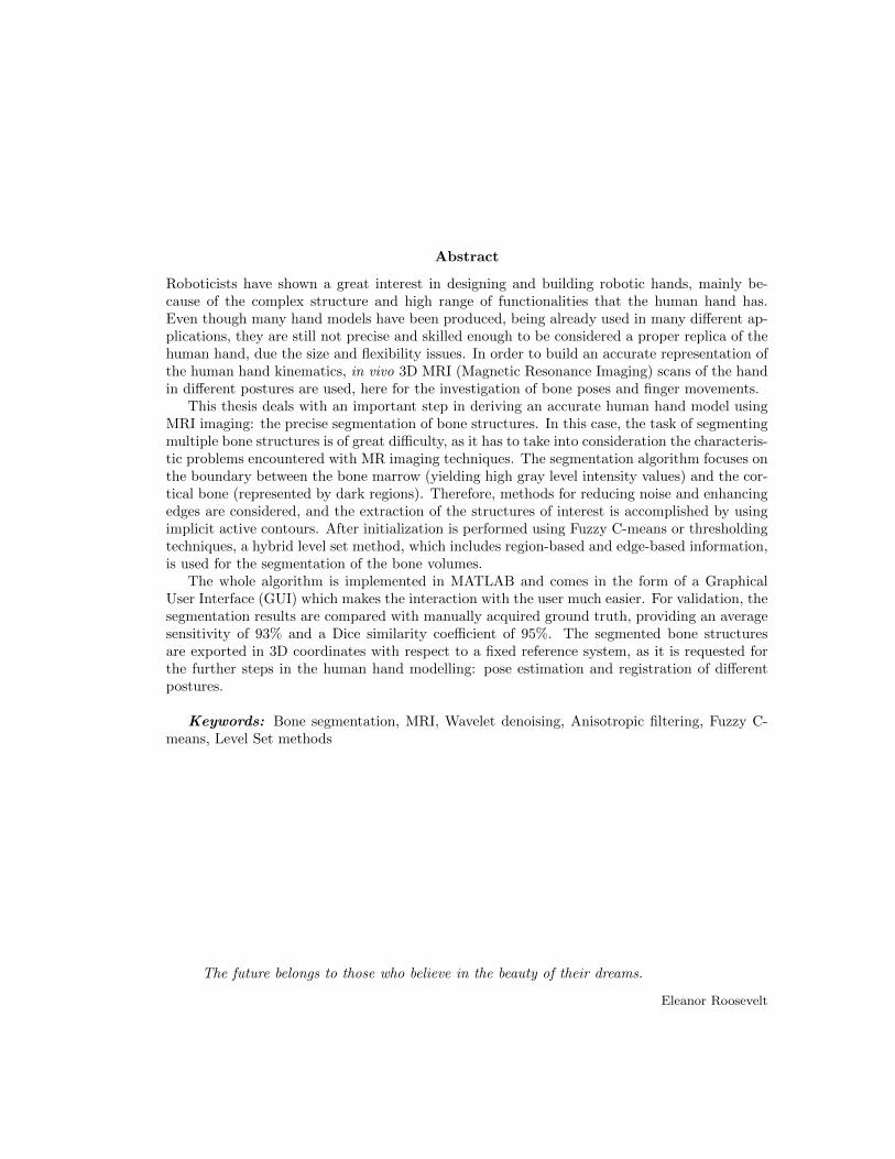
Abstract
Roboticists have shown a great interest in designing and building robotic hands, mainly be-cause of the complex structure and high range of functionalities that the human hand has.Even though many hand models have been produced, being already used in many different ap-plications, they are still not precise and skilled enough to be considered a proper replica of thehuman hand, due the size and flexibility issues. In order to build an accurate representation ofthe human hand kinematics, in vivo 3D MRI (Magnetic Resonance Imaging) scans of the handin different postures are used, here for the investigation of bone poses and finger movements.
This thesis deals with an important step in deriving an accurate human hand model usingMRI imaging: the precise segmentation of bone structures. In this case, the task of segmentingmultiple bone structures is of great difficulty, as it has to take into consideration the characteris-tic problems encountered with MR imaging techniques. The segmentation algorithm focuses onthe boundary between the bone marrow (yielding high gray level intensity values) and the cor-tical bone (represented by dark regions). Therefore, methods for reducing noise and enhancingedges are considered, and the extraction of the structures of interest is accomplished by usingimplicit active contours. After initialization is performed using Fuzzy C-means or thresholdingtechniques, a hybrid level set method, which includes region-based and edge-based information,is used for the segmentation of the bone volumes.
The whole algorithm is implemented in MATLAB and comes in the form of a GraphicalUser Interface (GUI) which makes the interaction with the user much easier. For validation, thesegmentation results are compared with manually acquired ground truth, providing an averagesensitivity of 93% and a Dice similarity coefficient of 95%. The segmented bone structuresare exported in 3D coordinates with respect to a fixed reference system, as it is requested forthe further steps in the human hand modelling: pose estimation and registration of differentpostures.
Keywords: Bone segmentation, MRI, Wavelet denoising, Anisotropic filtering, Fuzzy C-means, Level Set methods
The future belongs to those who believe in the beauty of their dreams.
Eleanor Roosevelt
Contents
Acknowledgments vii
1 Introduction 1
1.1 Motivation . . . . . . . . . . . . . . . . . . . . . . . . . . . . . . . . . . . . . . . 2
1.2 Objectives . . . . . . . . . . . . . . . . . . . . . . . . . . . . . . . . . . . . . . . . 3
2 Problem definition 5
2.1 Magnetic Resonance Imaging . . . . . . . . . . . . . . . . . . . . . . . . . . . . . 5
2.1.1 Noise in MR Imaging . . . . . . . . . . . . . . . . . . . . . . . . . . . . . 6
2.1.2 Partial volume effect . . . . . . . . . . . . . . . . . . . . . . . . . . . . . . 7
2.1.3 Intensity inhomogeneities . . . . . . . . . . . . . . . . . . . . . . . . . . . 8
2.2 The human hand . . . . . . . . . . . . . . . . . . . . . . . . . . . . . . . . . . . . 9
2.3 MRI datasets acquisition . . . . . . . . . . . . . . . . . . . . . . . . . . . . . . . . 10
3 Segmentation techniques applied in medical imaging 12
3.1 Intensity thresholding algorithms . . . . . . . . . . . . . . . . . . . . . . . . . . . 12
3.2 Region growing and Split and Merge algorithms . . . . . . . . . . . . . . . . . . . 14
3.3 Classification techniques . . . . . . . . . . . . . . . . . . . . . . . . . . . . . . . . 14
3.4 Clustering techniques . . . . . . . . . . . . . . . . . . . . . . . . . . . . . . . . . . 15
3.5 Atlas guided approaches . . . . . . . . . . . . . . . . . . . . . . . . . . . . . . . . 16
3.6 Mathematical morphology and Watersheds . . . . . . . . . . . . . . . . . . . . . 17
i
3.7 Active contours . . . . . . . . . . . . . . . . . . . . . . . . . . . . . . . . . . . . . 18
4 Methodology 21
4.1 Image pre-processing . . . . . . . . . . . . . . . . . . . . . . . . . . . . . . . . . . 21
4.1.1 Denoising MRI images using wavelets . . . . . . . . . . . . . . . . . . . . 21
4.1.2 Nonlinear anisotropic filtering . . . . . . . . . . . . . . . . . . . . . . . . . 24
4.2 Initialization . . . . . . . . . . . . . . . . . . . . . . . . . . . . . . . . . . . . . . 28
4.3 Level set methods . . . . . . . . . . . . . . . . . . . . . . . . . . . . . . . . . . . 30
4.3.1 Boundary-based level sets . . . . . . . . . . . . . . . . . . . . . . . . . . . 32
4.3.2 Region-based level sets . . . . . . . . . . . . . . . . . . . . . . . . . . . . . 33
4.3.3 Hybrid level set method . . . . . . . . . . . . . . . . . . . . . . . . . . . . 34
4.3.4 Optimization techniques for level set algorithms . . . . . . . . . . . . . . . 36
5 Results 38
5.1 Implementation . . . . . . . . . . . . . . . . . . . . . . . . . . . . . . . . . . . . . 38
5.2 Quality measures . . . . . . . . . . . . . . . . . . . . . . . . . . . . . . . . . . . . 44
5.3 Exporting the segmentation results . . . . . . . . . . . . . . . . . . . . . . . . . . 46
6 Conclusions 48
6.1 Conclusions . . . . . . . . . . . . . . . . . . . . . . . . . . . . . . . . . . . . . . . 48
6.2 Further work . . . . . . . . . . . . . . . . . . . . . . . . . . . . . . . . . . . . . . 49
Bibliography 57
ii

List of Figures
1.1 Example of an MRI image showing the type of tissues in the hand . . . . . . . . 4
2.1 Example of MRI image with added noise (a) Original MRI image (b) Crop from
the Original MRI image (c) MRI image with added Gaussian noise (d) MRI
image with Rician noise distribution . . . . . . . . . . . . . . . . . . . . . . . . . 7
2.2 Examples of the partial volume effect: (a) Synthetic image - the second image is
corrupted by the PVE, resulting in difficulties for the accurate boundary extrac-
tion between regions. [52], (b) A real MR image of a hand, affected by PVE. In
some regions of the image the boundary between the bone and the surrounding
tissue cannot be decided . . . . . . . . . . . . . . . . . . . . . . . . . . . . . . . . 8
2.3 Intensity inhomogeneities in MRI datasets:(a) Shaded region due to variability
of the magnetic field (white arrow) (b) Intensity distribution with respect to the
variability of the bone tissue . . . . . . . . . . . . . . . . . . . . . . . . . . . . . . 8
2.4 Histograms of the gray-level intensities of the same bone in different postures [61] 9
2.5 Configuration of the human hand [1]. . . . . . . . . . . . . . . . . . . . . . . . . 9
2.6 Configuration for the hand MRI sequence [62] . . . . . . . . . . . . . . . . . . . 10
2.7 Examples of postures of the hand . . . . . . . . . . . . . . . . . . . . . . . . . . . 11
3.1 Shape prediction using active contours . . . . . . . . . . . . . . . . . . . . . . . . 19
4.1 Thresholding of a linear signal using (b) Hard Thresholding or (c) Soft Thresholding 23
iii

4.2 Performance of an active geodesic contour algorithm (developed in Section 4.3.1)
on an image corrupted by Rician noise and its denoised versions using wavelets
and anisotropic diffusion . . . . . . . . . . . . . . . . . . . . . . . . . . . . . . . . 26
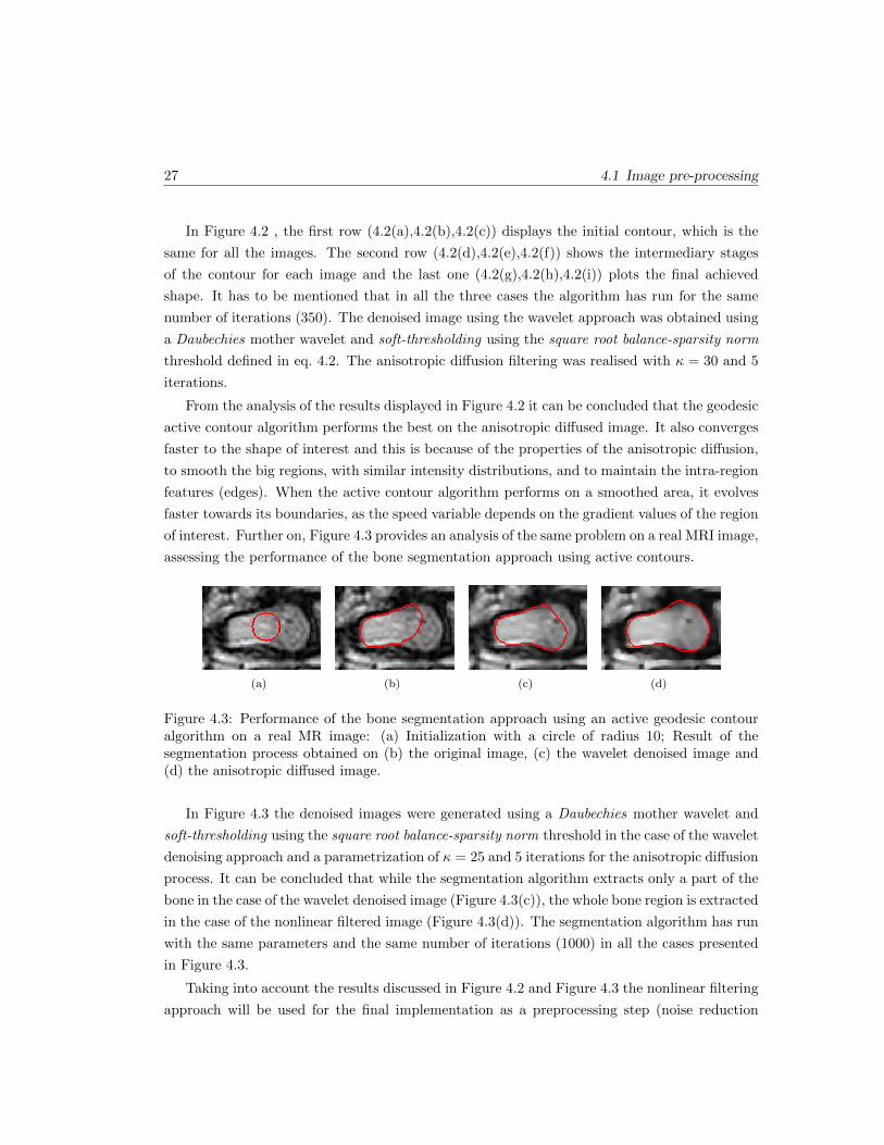
4.3 Performance of the bone segmentation approach using an active geodesic contour
algorithm on a real MR image: (a) Initialization with a circle of radius 10; Result
of the segmentation process obtained on (b) the original image, (c) the wavelet
denoised image and (d) the anisotropic diffused image. . . . . . . . . . . . . . . . 27
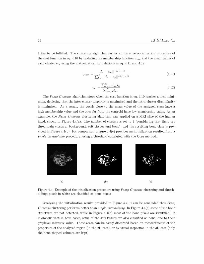
4.4 Example of the initialization procedure using Fuzzy C-means clustering and
thresholding; pixels in white are classified as bone pixels . . . . . . . . . . . . . . 29
4.5 Implicit representation of a circle of radius R, defining the contour Γ, the interior
domain Ω+ and the exterior domain Ω− . . . . . . . . . . . . . . . . . . . . . . . 30
4.6 (a) Level set conventions introduced in eq. 4.15 and 4.16 (b) Evolution of the
contour under the influence of the artificial forces [77] . . . . . . . . . . . . . . . 31
4.7 Comparison of the performances of the Chan Vese model and the proposed hybrid
model for the segmentation of the bone tissues in an MRI 2D slice . . . . . . . . 36
4.8 Example of how the narrow band is defined in the neighbourhood of the contour
and the need for reinitialization after the zero level set evolves . . . . . . . . . . . 36
5.1 Process flow . . . . . . . . . . . . . . . . . . . . . . . . . . . . . . . . . . . . . . . 38
5.2 Graphical User Interface (GUI) for 3D MRI data loading, pre-processing and
initialization . . . . . . . . . . . . . . . . . . . . . . . . . . . . . . . . . . . . . . . 39
5.3 Extraction of bone structures from volumes including bone and soft tissues using
the opening morphological operation . . . . . . . . . . . . . . . . . . . . . . . . . 40
5.4 Intermediate stage in the initialization process . . . . . . . . . . . . . . . . . . . 41
5.5 The result provided by the segmentation algorithm: (a) Initialization, (b) Final
segmentation . . . . . . . . . . . . . . . . . . . . . . . . . . . . . . . . . . . . . . 42
5.6 Grafical User Interface (GUI) for visualization of the MRI slices, the initial 2D
contours and the final segmented bone regions . . . . . . . . . . . . . . . . . . . . 43
iv

5.7 Comparison between the (a) initial contour and (b) the finally segmented bone
structures in a 2D MRI slice . . . . . . . . . . . . . . . . . . . . . . . . . . . . . . 43
5.8 Example defining the basic statistical measures using the comparison between
segmentation results and ground truth . . . . . . . . . . . . . . . . . . . . . . . . 44
5.9 Notations of the bones in the human hand . . . . . . . . . . . . . . . . . . . . . . 45
5.10 Computation of 3D coordinates using the geometry information provided by the
header of the DICOM file . . . . . . . . . . . . . . . . . . . . . . . . . . . . . . . 47
v

List of Tables
5.1 Quality measures for the 3D bone segmentation . . . . . . . . . . . . . . . . . . . 46
vi
Acknowledgments
First and foremost I would like to thank my thesis supervisor, Dipl. Ing. Georg Stillfried, for
allowing me to join the team of the DLR Bionics Group, for his expertise, kindness, and most
of all, for his patience. I found the weekly meetings with him and the Bionics Group very
interesting and constructive. Moreover, the support and pieces of advice received helped me to
successfully complete my master thesis.
I am also deeply grateful to the coordinators of the VIBOT Program: Prof. David Fofi,
Prof. Yohan Fougerolle, Prof. Fabrice Meriaudeau and Prof. Yvan Petillot. They offered me
the chance to join the Erasmus Mundus VIBOT Program, and I am grateful for their guidance
and support over the past 2 years. My gratitude also goes to the staff members involved
in the VIBOT course. Thank you for your cooperation and assistance in solving all kind of
administrative issues during all this period.
I am particularly thankful to Prof. Pere Ridao, who coordinated my internship in the
”Underwater Robotics Research Center” in Girona during the summer of 2010. This was a
significant period for me since I had the opportunity to further develop my technical and
personal skills.
The most special thanks go to my beloved parents, sister and girlfriend Isabel, who supported
and encouraged me during stressful moments. Their unconditional support throughout the
entire period was invaluable and this is the reason for which I devote this thesis to them.
Last but not least, I would like to thank my colleagues in the VIBOT 4 generation whose
spirit made these 2 years the best academic period I had so far. We had a lot of fun in all
vii

the places we visited and being together helped us to ride out all the difficulties (including
assignments, exams) we encountered.
viii

Chapter 1
Introduction
The human hand is one of the most complicated biomechanical structures of the human body.
It consists of bones, articulations, muscles, tendons, fat and skin. During the evolution, the
human hand expanded its functionalities, mainly related to the physical exploitation of the
environment. Due to its complex and delicate structure, it is able to carry out very accurate
grasping tasks (like picking up a needle) but also to accomplish activities which require gross
power skills (such as weight lifting). All these capabilities led to a high interest of roboticists in
designing and building robotic hands, which are able to copy the human hand kinematics and
dynamic characteristics.
A very elaborate and accurate model of the human hand can be applied in different do-
mains: from prostheses (where the human-like motion is of very high interest for cosmetic
reasons) to telemanipulation and service robotics (where the accuracy of the interaction with
the environment is important). Another skill which is widely studied in the literature is related
to the grasping accuracies. For an accurate modelling of the hand kinematics medical imaging
techniques are employed, and several steps have to be undertaken:
• Data acquisition: Firstly MR 3D image volumes have to be recorded in different postures.
The postures have to be as diversified as possible, so all the kinematic range can be
characterized.
• Segmentation: For each posture, extract the information from the 3D MR volume which
belongs to each bone structure.
• Pose estimation: Estimate the position and orientation of each bone with respect to a
reference coordinate system.
• Define the joint axes and identify the hand model: Estimate the type, position and
1
Chapter 1: Introduction 2
orientation of the joint axes, which optimally integrate the bone structures and derive
the kinematic chain based on their combination taking also into account the conciliation
between complexity and accuracy.
In this thesis, the analysis of the human hand structure is made from the medical image seg-
mentation point of view. Medical image segmentation refers to the extraction of the anatomical
structures of interest from digital images. The purpose is to accurately extract the bone struc-
ture of the human hand in different postures in order to be able to model a precise kinematic
model.
Image segmentation is a fundamental field in computer vision and many methods have been
developed with a view to deal with the limitations of the real-world studied datasets and the
varied requirements. Image segmentation algorithms can be easily classified in three groups: for
manual, semi-automatic and automatic segmentation. Manual segmentation is usually the most
precise technique, but it entails domain experts and it is very laborious and time consuming.
Also, the results of the manual segmentation procedures are affected by the subjective analysis
of the expert in charge. While semi-automatic segmentation algorithms need initialization
(some parameters or even regions of interest for the structures to be segmented), the automatic
algorithms have to extract the structures of interest independently, without any input from
the user. Besides, the results of the segmentation algorithms are affected by image artefacts
like noise, intensity inhomogeneities and low contrast between distinct regions. The problems
medical segmentation algorithms have to deal with are detailed in Section 2 and a general
introduction to the segmentation techniques applied in medical images with their advantages
and disadvantages is presented in Section 3.
1.1 Motivation
Most of the kinematic data used for hand modelling have been acquired using optical surface
markers. These surface markers are fastened to the skin and traced by optical measuring
systems (eg. Vicon). The estimated position and orientation of the markers in the calibrated
space, incorporated in a skeletal model, can help developing a good representation of the hand
kinematics. However , this approach experiences several drawbacks, one of the most important
ones being called the skin movement artefacts. It refers to the fact that the movement of
optical markers cannot totally and accurately describe the bone motion, mainly because of the
unmodellable and unstable movement of the soft tissue (skin).
This is the reason for which more accurate hand models are needed, which take into con-
sideration all the internal finger movements. This motivation leaded to conduct measurements
on hand cadavers, but it proved to be unreliable because of the rigidity of muscles or tendons,

3 1.2 Objectives
which would lead to errors in the kinematics representation. In order to handle the quality
requirements for the design of an accurate hand model, modern in vivo imaging techniques are
applied to record a high number of hand postures. The advantage of taking in vivo measure-
ments on awake subjects is that it offers the opportunity to study in detail the movement of
the bones and the behaviour of the soft tissues. Two medical imaging techniques offer high
resolution data essential for this type of analysis: MRI and CT.
Computed tomography (CT) is a non-invasive imaging technique, widely available, and use-
ful for the rapid visualization and localization of anatomic structures. The principle behind
CT scanning is that of conventional X-ray imaging, with ionizing radiation being emitted in
rotatory motion around the patient. This radiation passes through the tissue in multiple di-
rections, X-ray photon detectors measuring the degree of attenuation of the exiting radiation.
Then, the obtained data are integrated to produce images of scanned anatomical structure in
2D or 3D representation. This technique is more suitable for bone imaging, but because of the
radiation exposure it has been discarded.
Magnetic resonance imaging (MRI), on the other hand, is also a non-invasive imaging tech-
nique, which provides greater contrast in soft tissues without exposure to ionizing radiation. It
is based on the application of a powerful steady magnetic field, lining up the hydrogen atoms
in the tissue being imaged, and additional radio frequency fields, used to alter the alignment of
the magnetization, and to produce an effect detectable by the scanner. It is also able to carry
out 3D imaging of biological structures, but slower and at a lower resolution comparing with
CT.
In spite of the disadvantages it has with respect to CT imaging, MRI imaging is chosen
here, taking into account that no ionizing radiation is involved, which could give high risks for
the health of the subjects to be imaged, due to the large acquisition times.
1.2 Objectives
Around 50 hand postures from 3 different subjects were imaged using MRI sequences. The goal
of this thesis is to perform segmentation algorithms for the extraction of bone structures from
the 3D medical image volumes. It is of very high interest to either segment a fixed structure for
each bone in one posture, which is easy to distinguish in all the other datasets, or to segment
accurately each hand posture and then register the bones independently. This is needed for
the next step of the hand modelling, the pose estimation and registration between two different
poses. Usually the general segmentation algorithms are addressing a 2D problem and a special
interest on extending their capabilities to 3D datasets has been confirmed.
Segmenting bone regions in MRI data volumes is not a straightforward task, and the chal-
Chapter 1: Introduction 4
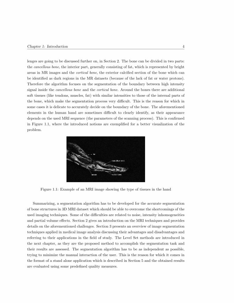
lenges are going to be discussed further on, in Section 2. The bone can be divided in two parts:
the cancellous bone, the interior part, generally consisting of fat, which is represented by bright
areas in MR images and the cortical bone, the exterior calcified section of the bone which can
be identified as dark regions in the MR datasets (because of the lack of fat or water protons).
Therefore the algorithm focuses on the segmentation of the boundary between high intensity
signal inside the cancellous bone and the cortical bone. Around the bones there are additional
soft tissues (like tendons, muscles, fat) with similar intensities to those of the internal parts of
the bone, which make the segmentation process very difficult. This is the reason for which in
some cases it is delicate to accurately decide on the boundary of the bone. The aforementioned
elements in the human hand are sometimes difficult to clearly identify, as their appearance
depends on the used MRI sequence (the parameters of the scanning process). This is confirmed
in Figure 1.1, where the introduced notions are exemplified for a better visualization of the
problem.
Figure 1.1: Example of an MRI image showing the type of tissues in the hand
Summarizing, a segmentation algorithm has to be developed for the accurate segmentation
of bone structures in 3D MRI dataset which should be able to overcome the shortcomings of the
used imaging techniques. Some of the difficulties are related to noise, intensity inhomogeneities
and partial volume effects. Section 2 gives an introduction on the MRI techniques and provides
details on the aforementioned challenges. Section 3 presents an overview of image segmentation
techniques applied in medical image analysis discussing their advantages and disadvantages and
referring to their applications in the field of study. The Level Set methods are introduced in
the next chapter, as they are the proposed method to accomplish the segmentation task and
their results are assessed. The segmentation algorithm has to be as independent as possible,
trying to minimize the manual interaction of the user. This is the reason for which it comes in
the format of a stand alone application which is described in Section 5 and the obtained results
are evaluated using some predefined quality measures.
Chapter 2
Problem definition
2.1 Magnetic Resonance Imaging
MRI is a non-invasive radiology technique generating anatomical and functional images of
the body, and particularly useful for neurological, oncological, cardiovascular, muscular and
skeletal imaging. Images can be obtained in any orientation, rapidly, non-invasively, and without
exposure to ionizing radiation. MRI technology is based on the application of a powerful steady
magnetic field, lining up the hydrogen atoms in the tissue being imaged, and additional radio
frequency fields, used to alter the alignment of the magnetization, and to produce an effect
detectable by the scanner. It allows for the variation of parameters such as repetition time (TR
- the time between two consecutive excitation pulses) and echo time (TE - the time between
the excitation pulse and the recording of the magnetization value).
Many pulse sequences are available in MR imaging techniques which leads to an optimization
problem. Depending on the anatomy of the structures of interest, the optimal pulse sequence has
to be chosen in order to be able to optimally distinguish the tissues of interest and to undertake
the segmentation procedure. For instance, MR imaging of brain tissues requires a specific
setup in comparison to bone analysis. Despite the non-ionizing radiation characteristics, MR
imaging experiences different imaging artefacts which generate difficulties for the segmentation
techniques having considerable effects on their performances [52]. Some of the drawbacks of
this imaging technique are: noise, low contrast between certain tissues, partial volume effects,
and intensity inhomogeneities. These shortcomings shall be discussed further on.
5
Chapter 2: Problem definition 6
2.1.1 Noise in MR Imaging
In magnetic resonance imaging (MRI) there is a trade off between signal-to-noise ratio (SNR),
acquisition time and spatial resolution. The SNR is relatively high in most MRI applications,
and this is accomplished implicitly and explicitly by averaging. The MRI data acquisition
process can be affected by two averaging techniques:
• Spatial volume averaging is required due to the discrete nature of the acquisition process;
• In the case of some applications, the signal for the same k-space location is acquired
several times and averaged in order to reduce noise.
The two averaging methods are interconnected. When a higher sampling rate of the fre-
quency domain is used, higher resolution images are obtained. However, in order to receive a
desired SNR at high spatial resolution a longer acquisition time is required, as additional time
for averaging is necessary. Conversely, the acquisition time, with the subsequent SNR and the
imaging resolution, are practically limited by the patient comfort and the system throughput.
Consequently, high SNR MRI images can be acquired at the expense of constrained temporal
or spatial resolution. Also, high resolution MRI imaging is achievable at a cost of lower SNR
or longer acquisition times.
Another important source of noise in MRI imaging is thermal noise in the human body.
Common MRI imaging involves sampling in the frequency domain (also called ”k-space”), and
the MRI image is computed using the Inverse Discrete Fourier Transform. Signal measurements
have components in both real and imaginary channels and each channel is affected by additive
white Gaussian noise. Thus, the complex reconstructed signal includes a complex white additive
Gaussian noise. Due to phase errors, usually the magnitude of the MRI signal is used for the
MRI image reconstruction. The magnitude of the MRI signal is real-valued and is used for
the image processing tasks, as well for visual inspection. Considering the received MRI signal
y[m,n] in eq. 2.1, where s[m,n] is the complex signal of interest and n[m,n] is the additive
complex Gaussian noise, the magnitude image at the pixel position m,n is computed using eq.
2.2, where θ represents the phase error of the received MRI signal and nr and ni are white
Gaussian noises.
y[m,n] = s[m,n] + n[m,n] (2.1)
x[m,n] = |y[m,n]| =√
(s[m,m] cos θ + nr[m,n])2 + (s[m,n] sin θ + ni[m,n])2 (2.2)
7 2.1 Magnetic Resonance Imaging
The way the magnitude MRI image is reconstructed results in a Rician distribution of the
noise. The main remark is that the Rician noise is signal-dependent, separating the signal
from noise being a very difficult task. In high intensity areas of the magnitude image, Rician
distribution can be approximated to a Gaussian distribution, and in low intensity regions it can
be estimated as a Rayleigh distribution. A practical effect is a reduced contrast of the MRI
image, as the noise increases the mean intensity values of the pixels in low intensity regions.
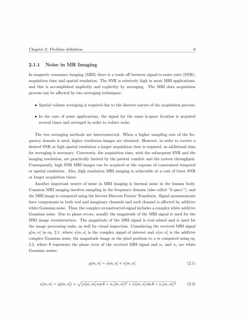
Figure 2.1 displays a comparison between the effect of Rician noise and Gaussian noise
added to a MRI image. It can be also noted that the adding of Gaussian noise produced some
negative data.
Figure 2.1: Example of MRI image with added noise (a) Original MRI image (b) Crop fromthe Original MRI image (c) MRI image with added Gaussian noise (d) MRI image with Riciannoise distribution
As explained, it is a fact that Rician noise degrades the MRI images in both qualitative and
quantitative senses, making image processing, interpretation and segmentation more difficult.
Consequently, it is important to develop an algorithm to filter this type of noise. Section
4.1 gives a comparison of two of the most used methods for MRI noise removal, and their
performances are assessed.
2.1.2 Partial volume effect
The partial volume effect (PVE) is the consequence of the limited resolution of the scanning
hardware and the discretization procedures. It occurs in non-homogeneous areas, where several
anatomical entities contribute to the gray-level intensity of a single pixel/voxel. It results in
blurred intensities across edges, making difficult the task of accurately deciding on the borders
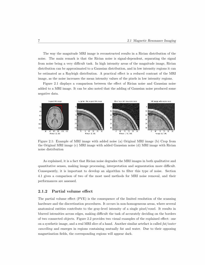
of two connected objects. Figure 2.2 provides two visual examples of the explained effect: one
on a synthetic image, and a real MRI slice of a hand. Another similar artefact is called fat/water
cancelling and emerges in regions containing mutually fat and water. Due to their opposing
magnetisation fields, the corresponding regions will appear dark.
Chapter 2: Problem definition 8
(a) (b)
Figure 2.2: Examples of the partial volume effect: (a) Synthetic image - the second image iscorrupted by the PVE, resulting in difficulties for the accurate boundary extraction betweenregions. [52], (b) A real MR image of a hand, affected by PVE. In some regions of the imagethe boundary between the bone and the surrounding tissue cannot be decided
2.1.3 Intensity inhomogeneities
Another difficulty which has to be handled by segmentation techniques using MR images is the
intensity inhomogeneities shortcoming. The intensity inhomogeneities can be caused by the
imperfections in the RF coil that produces the magnetic field, or by various harms in the signal
acquisition procedures. Also, the magnetic field can have a non-uniform distribution due to
the local magnetic properties of the studied biological structure or because of a movement of
the patient during the acquisition process. This effect can be identified as a shading artefact in
the image data and can have a major consequence on the performances of the intensity based
segmentation algorithms, considering that a certain tissue has a constant intensity distribution
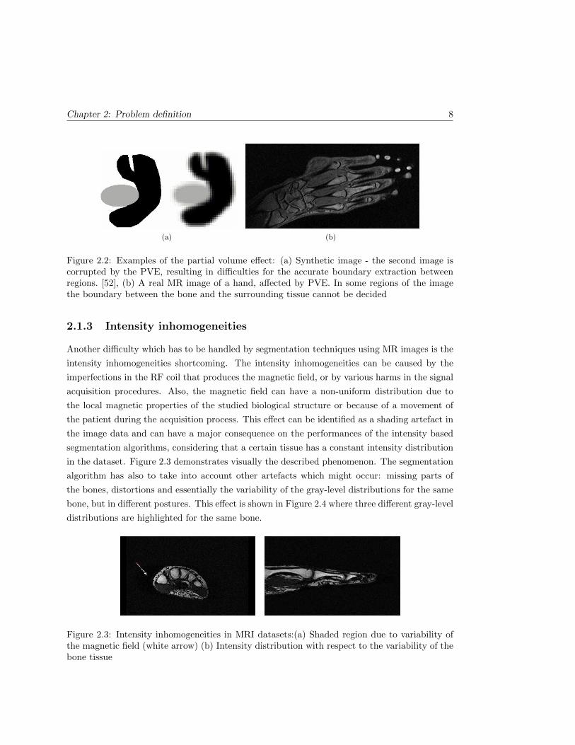
in the dataset. Figure 2.3 demonstrates visually the described phenomenon. The segmentation
algorithm has also to take into account other artefacts which might occur: missing parts of
the bones, distortions and essentially the variability of the gray-level distributions for the same
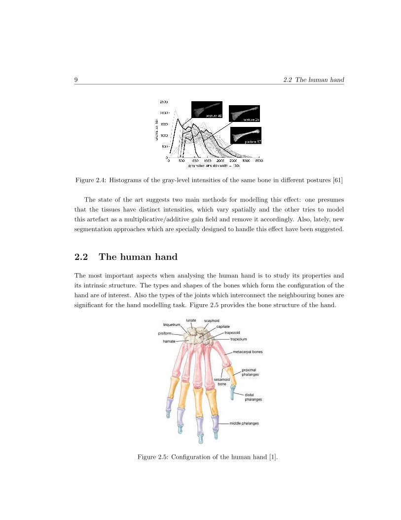
bone, but in different postures. This effect is shown in Figure 2.4 where three different gray-level
distributions are highlighted for the same bone.
Figure 2.3: Intensity inhomogeneities in MRI datasets:(a) Shaded region due to variability ofthe magnetic field (white arrow) (b) Intensity distribution with respect to the variability of thebone tissue
9 2.2 The human hand
Figure 2.4: Histograms of the gray-level intensities of the same bone in different postures [61]
The state of the art suggests two main methods for modelling this effect: one presumes
that the tissues have distinct intensities, which vary spatially and the other tries to model
this artefact as a multiplicative/additive gain field and remove it accordingly. Also, lately, new
segmentation approaches which are specially designed to handle this effect have been suggested.
2.2 The human hand
The most important aspects when analysing the human hand is to study its properties and
its intrinsic structure. The types and shapes of the bones which form the configuration of the
hand are of interest. Also the types of the joints which interconnect the neighbouring bones are
significant for the hand modelling task. Figure 2.5 provides the bone structure of the hand.
Figure 2.5: Configuration of the human hand [1].
Chapter 2: Problem definition 10
The human hand consists of a total of 27 bones, from which eight account for the carpus
(wrist), five are the metacarpal bones (creating the palm region) and the other fourteen are
called phalanges and define the structure of the fingers. The metacarpal bones have a cylindrical
shape and they articulate with the carpal bones on one side, and with the proximal phalanges
on the other side. The phalanges can be classified in 3 categories: five proximal phalanges at
the base of the fingers (the largest bones of the hand), four intermediate phalanges (one for each
finger, except the thumb) and the last, five distal phalanges (at the tip of the hand). Each finger
has a name for discerning reasons. Starting with the one closest to the thumb, they are named:
index, middle, ring and little (pinky) finger. In this thesis only the metacarpal bones and
phalanges are of interest, because they are the important parts of the hand structure providing
the motion functions. For the kinematics modelling analysis, the special configuration of the
joints is of higher importance, as they are essential for the wide range of hand configurations.
2.3 MRI datasets acquisition
Around 50 different postures of the hand on three subjects were scanned using a Philips Achieva
1.5T. A Philips SENSE 8-channel head coil was used for a higher signal-to-noise ratio and a
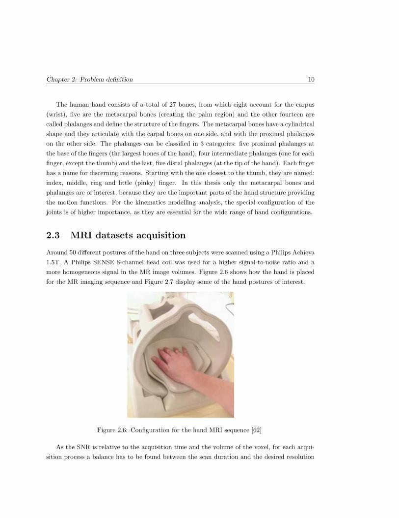
more homogeneous signal in the MR image volumes. Figure 2.6 shows how the hand is placed
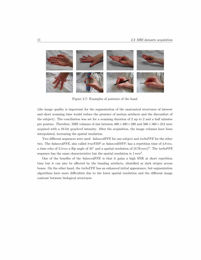
for the MR imaging sequence and Figure 2.7 display some of the hand postures of interest.
Figure 2.6: Configuration for the hand MRI sequence [62]
As the SNR is relative to the acquisition time and the volume of the voxel, for each acqui-
sition process a balance has to be found between the scan duration and the desired resolution
11 2.3 MRI datasets acquisition
Figure 2.7: Examples of postures of the hand
(the image quality is important for the segmentation of the anatomical structures of interest
and short scanning time would reduce the presence of motion artefacts and the discomfort of
the subject). The conciliation was set for a scanning duration of 2 up to 2 and a half minutes
per posture. Therefore, MRI volumes of size between 480× 480× 280 and 560× 560× 212 were
acquired with a 16-bit graylevel intensity. After the acquisition, the image volumes have been
interpolated, increasing the spatial resolution.
Two different sequences were used: balancedFFE for one subject and turboFFE for the other
two. The balancedFFE, also called trueFISP or balancedSSFP, has a repetition time of 4.8ms,
a time echo of 2.4ms a flip angle of 45 and a spatial resolution of (0.76mm)3. The turboFFE
sequence has the same characteristics but the spatial resolution is 1mm3.
One of the benefits of the balancedFFE is that it gains a high SNR at short repetition
time but it can also be affected by the banding artefacts, identified as dark stripes across
bones. On the other hand, the turboFFE has an enhanced initial appearance, but segmentation
algorithms have more difficulties due to the lower spatial resolution and the different image
contrast between biological structures.
Chapter 3
Segmentation techniques applied
in medical imaging
Advanced medical imaging techniques require high performance segmentation algorithms. The
main challenge in medical image segmentation tasks is to extract accurately the structures of
interest. In the case of medical imaging the segmentation process can take place in 2D or
in the 3D image domain. Usually 2D methods are applied on a single-image dataset and 3D
methods are used for volume segmentation. Nevertheless, 2D algorithms can be extended to 3D
medical volumes by being applied successively on the compounding 2D slices [7] [23] [38] [53].
The last approach is in some cases more practical as it is easier to implement, it requires less
memory, and has lower computation complexity. This section gives an overview of the 2D and
3D most common segmentation algorithms applied in medical imaging. An overview for the
implementation of each method is given and the advantages and disadvantages are discussed.
It has to be mentioned that often, depending on the task, several algorithms are combined
together with a view to solve difficult segmentation tasks.
3.1 Intensity thresholding algorithms
Thresholding is one of the easiest segmentation techniques for scalar images and volumes [55].
Mainly, it takes into account only the intensity value of the pixels or voxels and creates a
binary partition of the dataset. Single-threshold algorithms use only one intensity value, called
threshold, which separates the dataset into two classes as follows: intensities higher than the
threshold are clustered in one class and the rest of the pixels (or voxels) are clustered in the
other class. The mathematical formulation of the single-thresholding technique is shown in eq.
12
13 3.1 Intensity thresholding algorithms
3.1, where I is the analysed intensity value and λ is the threshold. This method is also called
binarization.
I =
0 if I ≤ λ1 if I > λ
(3.1)
When the analysed dataset contains more than 2 classes, a multi-thresholding algorithm has
to be applied. In case the dataset (image or volume) has to be clustered in n different classes,
n − 1 thresholds have to be applied. The corresponding formula is displayed in eq. 3.2 where
λ1 . . . λn−1 are the used threshold values for differentiating the dataset in n classes represented
by val1 . . . valn.
I =
val1 if I ≤ λ1
val2 if λ1 < I ≤ λ2
......
valn−1 if λn−2 < I ≤ λn−1
valn if I > λn−1
(3.2)
The difficult task is to determine the threshold values which best differentiate the regions
of interest. A simple case is the one in which the structures to be clustered have contrasting
intensity values (or other features). Practically, the resulting segmentation is very sensitive to
the used thresholds, noise and intensity inhomogeneities (present in MRI images). Another
important drawback of the approach is that it does not take into consideration the spatial
distribution of the intensities. However, this method can be implemented in real-time and it is
often used as an initialization step and combined with other segmentation techniques.
Adaptive thresholding is an approach which aims to improve the performance of the algo-
rithm in images corrupted by noise and intensity inhomogeneities (MRI images). Also called
local or dynamic thresholding methods [59], they compute a distinct threshold for each pixel
or voxel based on the local image properties. Kittler et al. [33] used the image statistics
based on the gradient magnitude for the selection of an automatic threshold, while Kom et.
al [34] applied adaptive threshold in order to segment dense masses in mammograms. Other
medical image segmentation applications include extracting edges and maintain only the ones
which respect some predefined similarity criteria [11], segmenting blood vessels [56], extracting
anatomical structures in MR images [32] and endoscopic images [66] or 3D bone segmentation
in CT scans [76].
Chapter 3: Segmentation techniques applied in medical imaging 14
3.2 Region growing and Split and Merge algorithms
Region growing is a method which uses a predefined ”growing” criteria (connectivity, intensity
distribution, edges in the image) [27] in order to extract a region of interest from a scalar
image or volume. Compared to the thresholding techniques, it includes information related to
the neighbourhood configuration and it is designed to extract homogeneous regions which have
higher probability to correspond to anatomical structures. It requires at least one seed point
for each object to be segmented, from which selects all the belonging pixels or voxels based
on the homogeneity criteria. Therefore, the main disadvantage is that it requires and is very
sensitive to initialization. Results of region growing algorithms are highly influenced by noise
and partial volume effects (specific for MRI images).
As in the case of the thresholding techniques, region growing is usually used in combination
with other more complex algorithms. For example Zhang et. al [76] used region growing as a
post-processing step for the 3D adaptive thresholding of the CT images. Also, CT angiographic
image segmentation has been realised using gradient based region growing [54]. Region growing
has been improved by including topological information for 3D MRI cortex segmentation [43]
or by adapting the algorithm to the fuzzy sets theory [67].
Split and merge algorithms are similar to region growing, but overcome the need of seed
points [44]. Similarly, based on a predefined criteria it successively splits the regions in a certain
number of subregions, and merges only the ones which satisfy the required conditions. The main
drawback of this algorithm is that it requires a pyramidal grid structure of the dataset, which
makes it very computationally expensive and undesirable for the huge array of data nowadays.
3.3 Classification techniques
Classifiers are usually used in pattern recognition tasks and their aim is to label the dataset
based on a feature space [8]. The used features for classification of the dataset is very varied,
some of the most common including image intensities or gradients. The main task when working
with classifiers is to find the feature space, which best describes the dataset and can easily
distinguish between the classes to be detected.
Classification techniques are known as supervised methods as they have to be first trained
with pre-segmented data and then tested on new datasets for the automatic segmentation
task [78]. Some of the most used classifiers in the literature are: k -nearest neighbour(kNN)
(each pixel or voxel is labelled as the same class in the training dataset which is the closest in
the feature space) or Parzen window (the labelling is realised based on a majority vote within a
region centred at the analysed pixel or voxel). These are non-parametric classifiers since in their
15 3.4 Clustering techniques
implementation no assumption is made with respect to the statistical structure of the dataset.
Maximum likelihood or Bayes classifier are common parametric classifiers. It is assumed that
the studied feature space is formed of independent samples which form a mixture of probability
distributions. Usually the distributions are Gaussian and the mixture is called finite mixture
model. When it is trained, the Bayes classifier estimates the K means, covariances and the
mixing coefficients, in the case of Gaussian mixtures. In the segmentation process, each pixel
or voxel receives the label with the highest posterior probability.
As mentioned, it is very important for the classifiers to work with distinct quantifiable fea-
tures. Practically, it is very difficult to find feature spaces which easily distinguish between the
classes to be labelled. Another drawback of these techniques is that they do not perform spatial
modelling, their results being vulnerable to noise corruption [70]. Also, manual interaction and
gathering of the training data are very time consuming and laborious. However, as they are
non-iterative, they are reasonably computationally effective and several feature spaces can be
combined in the classification process.
Maximum likelihood segmentation has been applied on ultrasound images [57] where the
density probability distribution and the smoothness constraints of the graylevel values are used
to define the energy functional. Vrooman et. al [68] implemented the conventional kNN in
combination with manual or atlas-based training for the brain tissue classification in multi-
spectral MRI images.
3.4 Clustering techniques
Clustering algorithms are known as unsupervised methods and perform the same task as
classifiers. The main difference is that they do not need training and they train themselves
using the offered dataset by iterating between segmenting the data and defining the properties
of each class. Common clustering algorithms are: K -means, fuzzy clustering and expectation-
maximization (EM) [16] [8] [40] [36]. The K -means algorithm computes the mean of the feature
space for each class and then allocates every pixel or voxel to the class with the closest feature
vector. The algorithm minimizes the dissimilarity of each class by iteratively reassigning the
pixels or voxels to the iteratively computed classes. Fuzzy c-means is a generalized version of
the K -means algorithm, which allows soft segmentation based on fuzzy set theory [75] [8]. The
expectation-maximization (EM) technique assumes that the data can be modelled as a mixture
of Gaussians and applies the same clustering procedure. It iteratively estimates the means,
covariances, mixing coefficients and computes the posterior probabilities.
Similar to classification techniques, no spatial distribution of the data is taken into account
Chapter 3: Segmentation techniques applied in medical imaging 16
in the clustering process, and thus their outcomes can be easily corrupted by noise and intensity
inhomogeneities. As they require initial parameters, sensitivity to initialization has been shown
in the literature. It also has been proved that EM has a higher initialization sensitivity in
comparison with K -means and fuzzy c-means clustering [74]. Nevertheless, improved robustness
to noise and intensity inhomogeneities has been demonstrated when these methods are combined
with other techniques like Markov random fields and Bayesian approaches [51] [25]. In order to
overcome the noise and inhomogeneity sensitivity, the performance of the clustering methods
has been improved using spatial information in the minimization function [69] [14]. One of the
most common application is the brain tissue segmentation in MR images [69].
Markov Random Field (MRF) Modelling is not a segmentation technique, but a statistical
scheme which is often used with other segmentation techniques for results improvement. The
main aim of the MRFs is to include the spatial information in the segmentation process by
modelling the relationships between neighbouring pixels or voxels [39]. For example, in medical
image processing, this method sets constraints on the interconnectivity between pixels or voxels
representing the same organ. In this case it is considered that most of the pixels or voxels can
be classified the same as their neighbours, because of the very low probability of existing organs
represented by a very low number of pixels/voxels.
The main disadvantages of this approach are the computational cost and the tuning of
the parameters managing the strength of the spatial relationships between pixels/voxels [39].
Selecting too high parameters would result an extremely smoothed segmentation loosing im-
portant details of the structures to be segmented. Nevertheless, these algorithms are widely
used in medical imaging processing, due to their ability to model also intensity inhomogeneities
which are widely present in MR images [28].
3.5 Atlas guided approaches
Atlas guided techniques are widely used in medical image analysis when templates or atlases
are accessible. An atlas is created using the anatomical information of the structure to be seg-
mented. Once the atlas is generated, it is used as a reference for the segmentation algorithm,
translating the process to a registration problem [42]. An initial step is to determine a transfor-
mation which maps a pre-segmented atlas structure to a configuration in the analysed image.
This procedure is called atlas warping and is usually achieved using linear transformations [5].
Occasionally, the algorithm adapts to the anatomical variability of the studied structure by
applying a sequence of linear and nonlinear transformations [15] [17] [18].
MR brain imaging is one of the most common applications of the Atlas guided approaches.
The great advantage is that during the segmentation process, the labels are also transferred to
17 3.6 Mathematical morphology and Watersheds
the studied dataset. On the other hand, these techniques have proved difficulties in segmenting
very complex structures. Also the results provided by these algorithms are affected by the vari-
ability of the anatomical structures between subjects. This is the reason for which their usage
is recommended for structures which are stable over the studied population. An improvement
has been proposed by Thompson and Toga [65] by using probabilistic atlases, but this approach
is more computationally expensive and requires manual interaction.
3.6 Mathematical morphology and Watersheds
Mathematical morphology is a technique for analysing geometrical structures in image process-
ing tasks. Originally defined only for binary datasets, their functions have been later enlarged
for the use on grayscale data. This technique measures how a predefined shape, called structur-
ing element, fits or misses the structures in the studied dataset. Examples of used structuring
elements in medical image analysis are discs, circles and squares (in the 2D case), and spheres
and cubes (in 3D) [58]. The choice of the structuring element is very significant for the seg-
mentation process, as the results strongly depend on the size and shape of the chosen local
neighbourhood template. Summarizing the basic procedures, the two main used morphologic
operations are dilation and erosion [45]. For example, having defined a 3×3 square structuring
element, as shown in eq. 3.3, the related dilation and erosion operations are described in eq. 3.4,
where A denotes the binary image to be analysed, φ is the empty set and y+ S = y+ s|sεS.
S = (i, j)εZ2|i, j = −1, 0, 1 (3.3)
Ds = yεZ2|y + S ∩A 6= φ,
Es = yεZ2|y + S ⊆ A (3.4)
The operators defined in eq. 3.4 can provide useful information on the edges and the bound-
aries of the existing structures in the analysed dataset, which can be further used in the seg-
mentation process. Also, the combination of the two operators provides two additional mor-
phological transformations: opening (erosion followed by dilation using the same structuring
element) and closing (dilation followed by erosion) [10]. Practically, using the closing trans-
formation, small holes or gaps are reduced; while opening removes narrow connectors (can
better distinguish the studied structures) or opens large holes. Morphological operators can
not be considered standalone segmentation techniques, but they are usually used as a step in
the segmentation workflow.
The morphological approach for medical image segmentation merges region growing and
Chapter 3: Segmentation techniques applied in medical imaging 18
edge detection algorithms. Pixels/voxels which are situated close to a regional minima of
the intensity function are grouped together and the borders between two neighbouring groups
are defined along the high gradient values of the image. This method is called watershed
transformation and its applicability has been extended to grayscale images as well. In the case
of a 2D image, based on the intensity value, every pixel can be classified in one of the three
groups:
• a) pixels placed in a local minimum
• b) pixels placed in the neighbourhood of a local minimum
• c) pixels placed equally between several local minimum points
For a particular local minimum, a catchement basin is formed from the set of pixels satisfying
the second condition (also called the watershed of the local minimum). The points belonging to
the third group are defining the watershed lines. The main goal of the watershed segmentation
techniques is to determine the catchement basins, whose local minima represent structures
of interest in the analysed image, and the watershed lines, providing the boundaries of the
structures. The great disadvantage of this approach is that usually it over-segments the images,
particularly in the case of noisy images (MRI datasets). This leads to additional pre-processing
or post-processing stages (for example to merge the resulted regions based on a similarity
criteria) which might require manual interaction, which is time consuming. Therefore, in order
to reduce over-segmentation, Najman and Schmitt [46] suggested the use of morphological
operators.
Dogdas et al. [19] proposed a sequence of morphological operations for the 3D skull segmen-
tation in MR images. Also, morphological operators have been widely used as a pre-processing
step for splitting connected distinct structures (it is also the case of two bones connected due
to the noise in the image dataset) [2]. Watershed techniques using prior information [26] and
probabilistic atlases [63] have been also successfully used in medical image segmentation tasks.
3.7 Active contours
Active contour methods can intuitively be understood as digitally-generated curves operating
within images with the aim of identifying object boundaries. Initially named snakes [31] , they
are energy minimizing splines, moulding a closed contour to image object boundaries by means
of deformation under the influence of image forces, internal forces and external constraint forces.
Considering that the snake (contour) position at time t can be parametrically represented
by v(s, t) = (x(s, t), y(s, t)), the evolution of the deformable model can be represented as shown
in eq. 3.5, where µ(s) and γ(s) control the mass and the damping density of the contour. The
19 3.7 Active contours
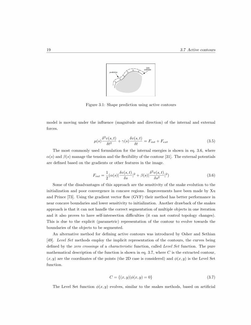
Figure 3.1: Shape prediction using active contours
model is moving under the influence (magnitude and direction) of the internal and external
forces.
µ(s)δ2v(s, t)
δt2+ γ(s)
δv(s, t)
δt= Fint + Fext (3.5)
The most commonly used formulation for the internal energies is shown in eq. 3.6, where
α(s) and β(s) manage the tension and the flexibility of the contour [31]. The external potentials
are defined based on the gradients or other features in the image.
Fint =1
2(α(s)|δv(s, t)
δs|2 + β(s)|δ
2v(s, t)
δs2|2) (3.6)
Some of the disadvantages of this approach are the sensitivity of the snake evolution to the
initialization and poor convergence in concave regions. Improvements have been made by Xu
and Prince [73]. Using the gradient vector flow (GVF) their method has better performance in
near concave boundaries and lower sensitivity to initialization. Another drawback of the snakes
approach is that it can not handle the correct segmentation of multiple objects in one iteration
and it also proves to have self-intersection difficulties (it can not control topology changes).
This is due to the explicit (parametric) representation of the contour to evolve towards the
boundaries of the objects to be segmented.
An alternative method for defining active contours was introduced by Osher and Sethian
[49]. Level Set methods employ the implicit representation of the contours, the curves being
defined by the zero crossings of a characteristic function, called Level Set function. The pure
mathematical description of the function is shown in eq. 3.7, where C is the extracted contour,
(x, y) are the coordinates of the points (the 2D case is considered) and φ(x, y) is the Level Set
function.
C = (x, y)|φ(x, y) = 0 (3.7)
The Level Set function φ(x, y) evolves, similar to the snakes methods, based on artificial
Chapter 3: Segmentation techniques applied in medical imaging 20
forces, which make the front move in the normal direction. The progressing contour can be
extracted at any moment from the zero level set, as shown in eq. 3.7. Some of the advantages of
the Level Sets in comparison with the snakes approach can be concluded: implicit representation
(no parametrization), allows changes in topology of the evolving contour and can easily represent
various geometrical shapes in different number of dimensions (2D and 3D).
Active contour methods have been widely applied in medical image segmentation tasks
[22] [21] [35]. Their ability to adapt contours to structures with irregular shapes made them
applicable for brain segmentation tasks [6] or tumour region detection. They were also used
for segmenting 3D volumetric MRI datasets for image guided surgery tasks [9]. Chunming
Li et al. [37] proposed an improvement of the variational level set methods in the case of
medical datasets corrupted by intensity inhomogeneities which has significant results on bone
segmentation in X-ray images. Jiang [29] combined in his work the active contours approach
with morphological operations for the X-ray bone fracture subtraction. Local structure [71]
and texture [41] descriptors have been also incorporated in the evolution of the active contours
for bone segmentation in CT datasets.
Chapter 4
Methodology
The implemented segmentation algorithm comprises several stages for the successful accom-
plishment of the task. The first step takes into account the pre-processing of the images to be
analysed for reducing the noise and enhancing the features of interest for the subsequent seg-
mentation algorithms. This stage is developed in section 4.1, where two widely used procedures
are compared, while the next section discusses initialization techniques. Finally, level set meth-
ods are introduced, as they are one of the most used techniques in medical image segmentation.
A hybrid level set model is proposed, which uses region and edge information for the contour
propagation, and several methods for speed and quality improvement are suggested. All the
considered procedures described in this chapter are implemented, and their results are shown
and investigated in chapter 5.
4.1 Image pre-processing
4.1.1 Denoising MRI images using wavelets
One of the important applications of wavelets is image denoising and compression. By com-
puting the Discrete Wavelet Transform (DWT) the image content is decomposed in scaling
coefficients (approximation sub-band) and wavelet coefficients (detail sub-band) at different
orientations (horizontal, vertical and diagonal) and resolutions. One of the characteristics of
the DWT is that it tends to concentrate the information contained in the analysed signal into
a relative small number of coefficients. In the case of a noisy image, the DWT will contain a
reduced number of coefficients with high SNR and many coefficients with low SNR. The main
noise reduction algorithm based on DWT decomposition is to discard low SNR coefficients and
to keep the significant ones. After selecting the desired coefficients, the Inverse Discrete Wavelet
21
Chapter 4: Methodology 22
Transform (IDWT) provides the noise suppressed image. Nevertheless, the DWT is not time
space invariant, simple miss-alignments between the signal and the wavelet basis function pro-
viding artefacts in the denoised image. This drawback is solved by using the Shift-invariant
Wavelet Transform (SWT). No development of the wavelet transform analysis will be made in
this section, as the purpose is only the applicability of the wavelet transform for denoising MRI
images. A detailed introduction in the wavelet theory can be found in [30]. Several properties
which make the wavelet transform suitable for the denoising task, are summarised below:
• multiresolution - the multi-level wavelet decomposition allows the analysis of image details
at different scales;
• edge detection - high wavelet coefficients correspond to image edges;
• edge evolution across scales - the wavelet coefficients corresponding to image edges tend
to persist across the scales.
The main task is to find a suitable threshold in order to select the coefficients which best
describe the information in the analysed image and to suppress as much noise as possible. In
the case the threshold is too low, the noise suppression might be unsatisfactory, but loss of
image detail (excessive smoothing) would be visible in the case of a high threshold.
Many techniques have been proposed in the literature with a view to find the best suitable
threshold for the wavelets coefficients and for noise level estimation in MRI images. A survey
of the methods used for noise estimation is given by Aja-Fernandes et al [4]. There are summa-
rized methods which are using background regions in the MRI image for the noise distribution
estimation [60] [3] as well as techniques which model the Rician noise distribution using the
square of the magnitude MRI image [47].
One of the most used method for denoising MRI images by thresholding the wavelet coef-
ficients is the one proposed by Donoho [20]. He showed that a global threshold, defined in eq.
4.1, is asymptotically optimal, where N is the size and σ is the noise standard deviation of the
wavelet coefficient arrays.
λ = σ√
2 logN (4.1)
Taking into account that the universal threshold is computed globally using the coefficients at
all scales, the resulting denoised images are usually over-smoothed. To overcome this problem,
the square root balance-sparsity norm approach can be used for defining an optimal threshold.
A thresholds array t is defined as having all the possible values uniformly distributed . Using
the t array, two curves are defined: the percentage of 2-norm recovery (the measure of the
energy loss after the denoising process using the values in t) and the percentage of the relative

23 4.1 Image pre-processing
sparsity (the number of resulting 0 coefficients in the denoised image). The two curves intersect
at the topt and the square root balance-sparsity norm threshold is defined using eq. 4.2.
λ =√topt (4.2)
After an optimal threshold is computed, it can be applied to the wavelet coefficients in two
different manners:
• Hard thresholding is the simplest method and it sets to zero all the coefficients which
are smaller than the threshold and keeps the others. Considering c the array of wavelet
coefficients to be thresholded, the mathematical definition is shown in eq. 4.3:
ch(k) =
sign(c(k))(|c(k)|) if |c(k)| > λ
0 if |c(k)| ≤ λ(4.3)
• Soft thresholding is an extension of the hard thresholding method, first discarding the
coefficients which are smaller than the threshold, and scaling the remaining ones. This
method has better mathematical properties because it does not create discontinuities at
c(k) = ±λ comparing the the hard procedure which does. The equation defining the soft
shrinkage rule is given in eq. 4.4:
cs(k) =
sign(c(k))(|c(k)| − λ) if |c(k)| > λ
0 if |c(k)| ≤ λ(4.4)
The effects of the thresholding methods defined in eq. 4.3 and 4.4 applied on a linear signal
can be visualized in Figure 4.1 (the used threshold is λ = 1 for a linear signal defined in the
range [0, 2]).
Figure 4.1: Thresholding of a linear signal using (b) Hard Thresholding or (c) Soft Thresholding
The proposed method for MRI image denoising using wavelets is summarised in Algorithm
1 and consists in the following steps:
Chapter 4: Methodology 24
Algorithm 1: MRI image denoising using wavelets
1. Choose a type of wavelet (’Haar’,’Daubechies’,’Symlets’,’Biorthogonal wavelets’) and the
number of levels of decomposition (scales) and compute the DWT (or SWT) of the image
to be denoised.
2. Compute an optimal threshold using eq. 4.1 or 4.2.
3. Select one of the shrinkage methods (eq. 4.3 and 4.4) and apply the threshold to the
wavelet coefficients accordingly.
4. Compute the IDWT (or ISWT) using the thresholded coefficients and determine the
denoised image.
4.1.2 Nonlinear anisotropic filtering
One common technique used in image processing to decrease the noise is the scale-space pro-
cedure firstly introduced by Witkin [72]. It refers to creating a family of images using the
convolution of the original image with an isotropic Gaussian filter of different widths. The
process is called linear diffusion and results in a family of increasingly blurred images, as the
standard deviation of the Gaussian kernel increases. This method has a main drawback as it
reduces the noise, it also degrades the details in the original image.
Perona and Malik [50] proposed a technique, called anisotropic diffusion, which reduces the
image noise but preserves or even enhances the features in the image (e.g. edges, lines) which are
of high interest in image processing tasks. The suggested filter can be expressed as a diffusion
process which gives preference to intra-region instead of inter-region smoothing. The novelty
is that the diffusive procedure is controlled by a variable diffusion coefficient, which limits the
smoothing in areas of interest (edges, boundaries). The general mathematical formulation of
the mentioned technique is given in eq. 4.5, where c(x, y, t) is the diffusion coefficient, I(x, y, t)
is the image intensity and div and ∇ are the divergence and the gradient operators. The spatial
coordinates of the image are represented by x and y (in the 2D case), and t corresponds to the
time parameter, which in discrete implementation is the iteration number.
∂
∂tI(x, y, t) = div(c(x, y, t)∇I(x, y, t)) (4.5)
The main difficulty is to choose the proper diffusion coefficient. It is defined as a positive
monotonically decreasing function of the image gradient which, ideally, has to be 0 at edges and
1 when the filter is located at the interior of a region. Practically, c(x, y, t) has to encourage the
25 4.1 Image pre-processing
forward diffusion inside smooth regions (small variations like noise and useless texture have to
be removed), and backward diffusion at high gradient locations (preserving and even sharpening
the boundaries and the features of interest). Perona and Malik [50] proposed two mathematical
functions for the diffusion coefficient, where the first one (eq. 4.6) advantages the high contrast
edges rather than the low contrast ones, and the second one (eq. 4.7) favours the wide areas
instead of narrow ones.
c1(x, y, t) = exp
(−(|∇I(x, y, t)|
κ
)2)
(4.6)
c2(x, y, t) =1
1 +
(|∇I(x, y, t)|
κ
)2 (4.7)
In eq. 4.6 and 4.7 κ is called the conductance parameter and has to be chosen accordingly
so the anisotropic diffusion process can distinguish between an edge and an intensity value
corrupted by noise. Usually it is selected empirically, or, when it is the case, it is defined using
a noise estimator.
The numerical scheme which implements the eq. 4.5 defines the intensity change at location
(x, y) after one iteration as a sum of contributions of the neighbouring pixels weighted by the
corresponding directed flow components (defined in eq. 4.8), as shown in eq. 4.9.
ΦE(x, y, t) = c(x+dx
2, y, t)[I(x+ dx, y, t)− I(x, y, t)]
ΦW (x, y, t) = c(x− dx
2, y, t)[I(x, y, t)− I(x− dx, y, t)]
ΦN (x, y, t) = c(x, y +dy
2, t)[I(x, y + dy, t)− I(x, y, t)]
ΦS(x, y, t) = c(x, y − dy
2, t)[I(x, y, t)− I(x, y − dy, t)] (4.8)
I(x, y, t+ dt) = I(x, y, t) + dt
[1
dx2[ΦE(x, y, t)− ΦW (x, y, t)] +
1
dy2[ΦN (x, y, t)− ΦS(x, y, t)]
](4.9)
It has to be mentioned that in eq. 4.8 and 4.9 dx and dy represent the pixel spacing in
the intensity image accounting for the anisotropy of the procedure. This suggests that, at a
certain location, closer pixels contribute more than the ones located at a higher distance. Also,
the aforementioned numerical scheme refers to a 4-pixel connectivity. For a better isotropy,
Chapter 4: Methodology 26
it can be easily extended to 8-pixel connectivity, by adding the contribution of the diagonal
neighbouring pixels (placed at a distance√dx2 + dy2) or even to 26-pixel connectivity in the
case of 3D image datasets. In eq. 4.9 the integration constant dt is introduced. For numerical
stability reasons it has to be chosen with respect to a stability criteria. It depends on the
number of neighbouring pixels/voxels and a full list of integration constants, considering the
connectivity structure, is provided in [24] .
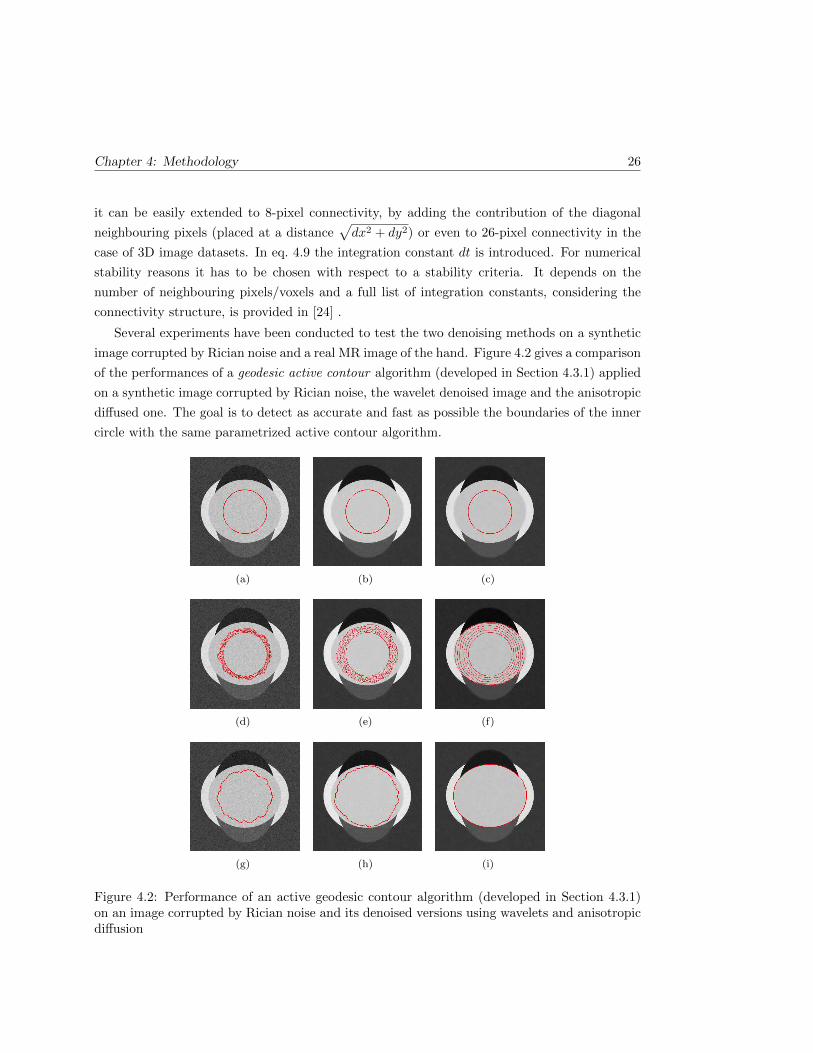
Several experiments have been conducted to test the two denoising methods on a synthetic
image corrupted by Rician noise and a real MR image of the hand. Figure 4.2 gives a comparison
of the performances of a geodesic active contour algorithm (developed in Section 4.3.1) applied
on a synthetic image corrupted by Rician noise, the wavelet denoised image and the anisotropic
diffused one. The goal is to detect as accurate and fast as possible the boundaries of the inner
circle with the same parametrized active contour algorithm.
(a) (b) (c)
(d) (e) (f)
(g) (h) (i)
Figure 4.2: Performance of an active geodesic contour algorithm (developed in Section 4.3.1)on an image corrupted by Rician noise and its denoised versions using wavelets and anisotropicdiffusion
27 4.1 Image pre-processing
In Figure 4.2 , the first row (4.2(a),4.2(b),4.2(c)) displays the initial contour, which is the
same for all the images. The second row (4.2(d),4.2(e),4.2(f)) shows the intermediary stages
of the contour for each image and the last one (4.2(g),4.2(h),4.2(i)) plots the final achieved
shape. It has to be mentioned that in all the three cases the algorithm has run for the same
number of iterations (350). The denoised image using the wavelet approach was obtained using
a Daubechies mother wavelet and soft-thresholding using the square root balance-sparsity norm
threshold defined in eq. 4.2. The anisotropic diffusion filtering was realised with κ = 30 and 5
iterations.
From the analysis of the results displayed in Figure 4.2 it can be concluded that the geodesic
active contour algorithm performs the best on the anisotropic diffused image. It also converges
faster to the shape of interest and this is because of the properties of the anisotropic diffusion,
to smooth the big regions, with similar intensity distributions, and to maintain the intra-region
features (edges). When the active contour algorithm performs on a smoothed area, it evolves
faster towards its boundaries, as the speed variable depends on the gradient values of the region
of interest. Further on, Figure 4.3 provides an analysis of the same problem on a real MRI image,
assessing the performance of the bone segmentation approach using active contours.
(a) (b) (c) (d)
Figure 4.3: Performance of the bone segmentation approach using an active geodesic contouralgorithm on a real MR image: (a) Initialization with a circle of radius 10; Result of thesegmentation process obtained on (b) the original image, (c) the wavelet denoised image and(d) the anisotropic diffused image.
In Figure 4.3 the denoised images were generated using a Daubechies mother wavelet and
soft-thresholding using the square root balance-sparsity norm threshold in the case of the wavelet
denoising approach and a parametrization of κ = 25 and 5 iterations for the anisotropic diffusion
process. It can be concluded that while the segmentation algorithm extracts only a part of the
bone in the case of the wavelet denoised image (Figure 4.3(c)), the whole bone region is extracted
in the case of the nonlinear filtered image (Figure 4.3(d)). The segmentation algorithm has run
with the same parameters and the same number of iterations (1000) in all the cases presented
in Figure 4.3.
Taking into account the results discussed in Figure 4.2 and Figure 4.3 the nonlinear filtering
approach will be used for the final implementation as a preprocessing step (noise reduction
Chapter 4: Methodology 28
and edge enhancement). It has been proved that the anisotropic diffusion has several advan-
tages in comparison to the wavelet denoising procedure. The diffusive technique produces more
smoothed big regions (with similar intensity distributions) which help the active contour algo-
rithm to converge faster. Also it does not have any constraints on the size of the image to be
analysed; the wavelet denoising procedure requests that the image sizes have to be multiple of
2L, where L is the number of decomposition levels (in all the conducted tests, 4 scales were
used). This requirement limits the use of this procedure for cropped images or for analysing
images which do not respect the demanded condition. Finally, the anisotropic filtering method
can be easily expanded to 3D image datasets (26-connectivity).
4.2 Initialization
For a good segmentation of the bone structures in the MRI 3D datasets, an appropriate initial-
ization is required. It does not have to be very accurate, but it has to provide starting contours
(or volumes for the 3D case) for each bone to be segmented. Two elementary approaches
are considered for this stage: thresholding, using the single-thresholding method explained in
Section 3.1, or clustering using Fuzzy C-means.
Thresholding is a straightforward procedure. Based on visual inspection of the distribution
of the graylevel intensity values in the 3D image volume, the user has to select a threshold which
would distinguish the best between bone structures and the surrounding tissues. As mentioned
in Section 3.1, it is very difficult to determine a good threshold value and this process is very
sensitive to noise and intensity inhomogeneities.
Fuzzy C-means clustering is a method which allows the splitting of a dataset into several
classes. The user has to set the number of desired clusters, and every pixel/voxel in the dataset,
based on its features, is assigned to the closest class. This technique has been widely used in
medical image segmentation tasks, and the clustering of the pixels/voxels is derived from their
graylevel intensity values. Considering that each cluster is characterized by its mean value vm
and In is the intensity gray value of a pixel/voxel, Fuzzy C-means clustering implements the
minimization of the cost function in eq. 4.10, where µmn is a membership function, specific to
the fuzzy theory, which defines the degree of membership of the nth pixel/voxel to the mth class
(n = 1..N , where N is the number of pixels/voxels in the dataset and m = 1..C is the cluster
number). The degree of fuzziness of the resulting segmentation is decided by the l parameter,
with 1 ≤ l <∞.
J =
N∑n=1
C∑m=1
µlmn||In − vm||2 (4.10)
The membership function µmn is defined in the [0, 1] interval and the constraint∑Cm=1 µmn =
29 4.2 Initialization
1 has to be fulfilled. The clustering algorithm carries an iterative optimization procedure of
the cost function in eq. 4.10 by updating the membership function µmn and the mean values of
each cluster vm using the mathematical formulations in eq. 4.11 and 4.12.
µmn =||In − vm||−2/(l−1)∑Ck=1 ||In − vk||−2/(l−1)
(4.11)
vm =
∑Nn=1 µ
lmnIn∑N
n=1 µlmn
(4.12)
The Fuzzy C-means algorithm stops when the cost function in eq. 4.10 reaches a local mini-
mum, depicting that the inter-cluster disparity is maximised and the intra-cluster dissimilarity
is minimized. As a result, the voxels close to the mean value of the assigned class have a
high membership value and the ones far from the centroid have low membership value. As an
example, the Fuzzy C-means clustering algorithm was applied on a MRI slice of the human
hand, shown in Figure 4.4(a). The number of clusters is set to 3 (considering that there are
three main clusters: background, soft tissues and bone), and the resulting bone class is pro-
vided in Figure 4.4(b). For comparison, Figure 4.4(c) provides an initialization resulted from a
single-thresholding procedure, using a threshold computed with the Otsu method.
(a) (b) (c)
Figure 4.4: Example of the initialization procedure using Fuzzy C-means clustering and thresh-olding; pixels in white are classified as bone pixels
Analysing the initialization results provided in Figure 4.4, it can be concluded that Fuzzy
C-means clustering performs better than single-thresholding. In Figure 4.4(c) some of the bone
structures are not detected, while in Figure 4.4(b) most of the bone pixels are identified. It
is obvious that in both cases, some of the soft tissues are also classified as bone, due to their
graylevel intensity value. These areas can be easily discarded based on measurements of the
properties of the analysed region (in the 2D case), or by visual inspection in the 3D case (only
the bone shaped volumes are kept).

Chapter 4: Methodology 30
4.3 Level set methods
Level set methods were firstly introduced by Osher and Sethian [49] and have been widely used
in medical image segmentation applications, mainly because of their ability of tracking the
boundaries of the biological structures of interest. Some of their facilities include the intrinsic
representation of the contours which provides flexibility to topological changes, and their su-
perior numerical stability, which make them suitable for the extension of their applicability to
3D datasets.
When referring to implicit representation, it means that a contour Γ(t), which is supposed
to evolve towards the boundaries of the desired object, is defined as the zero level set of an
embedding-function φ(x, y, t) : R3× → R as given in eq. 4.13.
Γ(t) = (x, y)|φ(x, y, t) = 0 (4.13)
Using the contour defined in eq. 4.13, other two domains can be defined: Ω+ = (x, y)|φ(x, y, t) >
0, called the interior of Γ, and Ω− = (x, y)|φ(x, y, t) < 0, named the exterior of Γ.
Figure 4.5: Implicit representation of a circle of radius R, defining the contour Γ, the interiordomain Ω+ and the exterior domain Ω−
In the case of Figure 4.5 the embedding-function is defined on the whole domain as φ =
R2 − x2 + y2 and the contour Γ is defined as the zero level set of φ.
In practice the Level Set function φ(x, y, t) is generated using the signed Euclidean distance
function. The distance d(x, y) is defined as the length of the shortest path form the point (x, y)
to the contour Γ. Therefore, the interface can be defined as shown in eq. 4.14:
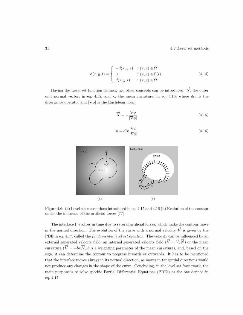
31 4.3 Level set methods
φ(x, y, t) =
−d(x, y, t) : (x, y) ∈ Ω−
0 : (x, y) ∈ Γ(t)
d(x, y, t) : (x, y) ∈ Ω+
(4.14)
Having the Level set function defined, two other concepts can be introduced:−→N , the outer
unit normal vector, in eq. 4.15, and κ, the mean curvature, in eq. 4.16, where div is the
divergence operator and |∇φ| is the Euclidean norm.
−→N = − ∇φ
|∇φ|(4.15)
κ = div∇φ|∇φ|
(4.16)
(a) (b)
Figure 4.6: (a) Level set conventions introduced in eq. 4.15 and 4.16 (b) Evolution of the contourunder the influence of the artificial forces [77]
The interface Γ evolves in time due to several artificial forces, which make the contour move
in the normal direction. The evolution of the curve with a normal velocity−→V is given by the
PDE in eq. 4.17, called the fundamental level set equation. The velocity can be influenced by an
external generated velocity field, an internal generated velocity field (−→V = Vn
−→N ) or the mean
curvature (−→V = −bκ
−→N ; b is a weighting parameter of the mean curvature), and, based on the
sign, it can determine the contour to progress inwards or outwards. It has to be mentioned
that the interface moves always in its normal direction, as moves in tangential directions would
not produce any changes in the shape of the curve. Concluding, in the level set framework, the
main purpose is to solve specific Partial Differential Equations (PDEs) as the one defined in
eq. 4.17.
Chapter 4: Methodology 32
∂φ
∂t+−→V |∇φ| = 0; (4.17)
Due to their applicability in medical image segmentation tasks, several types of active con-
tour models appear in the literature. A rough classification can divide the active contours
models in two classes: boundary-based and region-based. Each of these models have their own
advantages and disadvantages, depending on the segmentation task, which will be further on
explained.
4.3.1 Boundary-based level sets
Boundary-based level set methods are active contours which take into account the image in-
trinsics for the evolution of the curve towards the boundary of the object to be detected. A
representative implementation using this approach is the one proposed by Caselles et. al. [12]
which performs contour length minimization in a Riemannian space making use of intrinsic
geometric data in the image space. One of the advantages of this method is that it is a fusion
of the classical energy minimization approach introduced by snakes (discussed in Section 3.7)
and the theory of contour propagation using geometric information, providing high and stable
boundary localization. The curve evolution PDE proposed by Caselles et. al. [12] is formulated
in eq. 4.18, where I is the image domain and c is a non-negative real constant.
∂φ
∂t= g(I)|∇φ|div
(∇φ|∇φ|
)+ c∇g(I)|∇φ|
= g(I)(c+ κ)|∇φ| (4.18)
The evolution of the curve is influenced by a general-edge detector function, g(I), which
generates an image dependent force. The objective of this term is to accurately lead the
evolution of the curve toward the desired boundaries, and to stop the progress once the borders
are achieved. It can be defined in different manners, depending on the features of interest in
the image, with the condition that it has to be positive defined and monotonically decreasing
such that,
limz→∞
g(z) = 0 (4.19)
One common edge-indicator function, depending on the image gradient, is displayed in eq.
4.20, where Gσ ∗ I(x, y) is a smoothed version of the image using a Gaussian of σ standard
deviation and p ≥ 1 (the higher p, the steeper edge-indicator function). It has to be noted that
g complies with the condition in eq. 4.19. This implies that for high gradients in the image (at
33 4.3 Level set methods
edges), g = 0 and the curve evolution stops as it converges towards the desired boundaries.
g(|∇I(x, y)|) =1
1 + |∇Gσ(x, y) ∗ I(x, y)|p(4.20)
Another term of high importance in eq. 4.18 is (c+κ)|∇φ| which makes the level set moving
in the normal direction of the curve acting as an internal force. The mean curvature κ helps
the smoothing and the length minimization of the interface, as it incorporates geometrical
information, and the constant parameter c creates a balloon force which pulls the front in the
direction of the desired objects and also facilitates the capture of concave shapes.
In this approach the resulting segmented object is influenced only by the gradients in the
image. This can lead to defective results of the segmentation algorithm, as the contour can
stop at a local minimum (as high gradients can be placed anywhere in the image, especially in
the case of noisy images) or can ”leak” out of the structure of interest in a region where the
boundaries are not well defined. For these reasons, this segmentation technique is consistent
when it is applied on datasets where the edges of the structures to be segmented represent the
salient features.
4.3.2 Region-based level sets
Region-based level set methods try to deal with the leakage problem based on the Mumford-
Shah functional which attempts to split the image in two distinct regions (foreground and
background) based on a statistical approach. One of the most representative techniques which
implements level set evolution using region information is the Chan Vese model [13]. The
functional describing this model is shown in eq. 4.21.
ε(φ, µint, µext) = λ1
∫Ω
(I−µint)2H(φ)dΩ+λ2
∫Ω
(I−µout)2(1−H(φ))dΩ+α
∫Ω
H(φ)dΩ+β
∫Ω
|∇H(φ)|dΩ
(4.21)
The first two terms in eq. 4.21 refer to the distribution of the intensity levels in the exterior
and the interior of the level set, which are represented by the mean values of the two regions
(eq. 4.22), the third one refers to the area inside the level set and the last term represents the
length of the curve. H(φ) is the Heaviside function described in eq. 4.23, being 1 in the inner
region and 0 otherwise. The image domain is represented by Ω and α ≥ 0,β ≥ 0,λ1 > 0,λ2 > 0
are fixed parameters.
Chapter 4: Methodology 34
µint =
∫ΩIH(φ)dΩ∫
ΩH(φ)dΩ
µext =
∫ΩI(1−H(φ))dΩ∫
Ω(1−H(φ))dΩ
(4.22)
H(φ) =
0, if φ < 0
1, if φ ≥ 0(4.23)
Using the previously defined functional (eq. 4.21) the associated partial differential equation
describing the evolution of the level set is derived in eq. 4.24, with the Dirac function δ(φ) =∂H(φ)
∂φ.
∂φ
∂t= δ(φ)
[λ2(I − µext)2 − λ1(I − µint)2 − α+ βdiv
(∇φ|∇φ|
)](4.24)
The mean intensity values for the inner and outer regions, µint and µext, of the level set are
not previously defined. They are computed from the initialization of the curve and updated
after each iteration. For each point, the distance to the two mean values is computed, and
the curve is moved in such a way that the point is assigned to the region with the closest
average intensity value. The algorithm is considered to converge when, after the mean values
are updated, no points are reassigned. When the solution acquires the steady state, the contour
which best separates the two regions (background and foreground) is determined by the zero
level set of the embedding function φ.
This approach has many advantages over the edge-based approach. It is robust when seg-
menting regions with high noise, it can identify regions with fuzzy boundaries (very smooth)
and does not need any prior knowledge of the region to be segmented (mean intensity value).
On the other hand, it is limited to the segmentation of two regions (foreground and background)
and the global character of the mean values µint and µext may lead to erroneous segmentation
of objects with complex distributions of the intensity values.
4.3.3 Hybrid level set method
For an accurate segmentation of the bone structures in the MRI datasets, a hybrid level set
approach is employed. The main scope is to combine the capabilities offered by the region-based
and the edge-based level set methods in the interest of obtaining good segmentation results on
real MR images. This procedure was introduced by Zhang et. al [77] and the proposed partial
differential equation which describes the evolution of the contour is given in eq. 4.25, where
35 4.3 Level set methods
µ denotes the lowest graylevel intensity value which distinguishes the object to be segmented
from the background, and g = g(|∇I|) is the edge-indicator function introduced in eq. 4.20.
∂φ
∂t= δ(φ)
[α(I − µ) + βdiv
(g∇φ|∇φ|
)](4.25)
In the PDE given by eq. 4.25 the first term includes the region-based level sets approach,
advancing the contour towards areas with graylevel intensity values higher than µ, and the
second expression comprises the edge-based method which makes the interface evolve in the
direction of high image gradients. The contribution of each term of the PDE to the evolution
of the level set embedding function is weighted using the parameters α and β. Using the
PDE proposed by Zhang et al. in eq. 4.25 and the Chan Vese model proposed in eq. 4.24 the
functional for the aforementioned hybrid model can be defined in eq. 4.26.
∂φ
∂t= δ(φ)
[λ2(I − µext)2 − λ1(I − µint)2 + βdiv
(g∇φ|∇φ|
)](4.26)
This curve evolution described in eq. 4.26 allows the level set algorithm to evolve inside the
object of interest, but restricts the progress at high image gradients and also smooths the curve
at weak edges. Another situation which has to be taken into account when trying to segment
bone structures in MR images is the non-uniform intensity distribution of the graylevel values.
This can be solved by including information regarding the variance of the segmented objects in
the evolution function (as proposed by [48]). The PDE describing the hybrid level set model
which combines boundary and region, as well as, statistical information is given in eq. 4.27,
with the variance mathematical formulations displayed in eq. 4.28.
∂φ
∂t= δ(φ)
[λ2
(I − µext)2
σ2ext
− λ1(I − µint)2
σ2int
− log σ2ext
σ2int
+ βdiv
(g∇φ|∇φ|
)](4.27)
σ2int =
∫Ω
(I − µint)2H(φ)dΩ∫ΩH(φ)dΩ
σ2ext =
∫Ω
(I − µext)2(1−H(φ))dΩ∫Ω
(1−H(φ))dΩ(4.28)
Figure 4.7 provides a visualization of the segmentation results provided by the Chan Vese
model and the proposed hybrid model (which includes both region and edge information). In
Figure 4.7(a) it can be seen that in the case of the first proximal phalanx the segmentation algo-
rithm ”leaks”, including in the segmented area a part of the neighbouring soft tissue (indicated
with the white arrow). This issue is solved in the mathematical formulation of the hybrid level
set as shown in Figure 4.7(b). The term comprising edge-based information is dominant in the
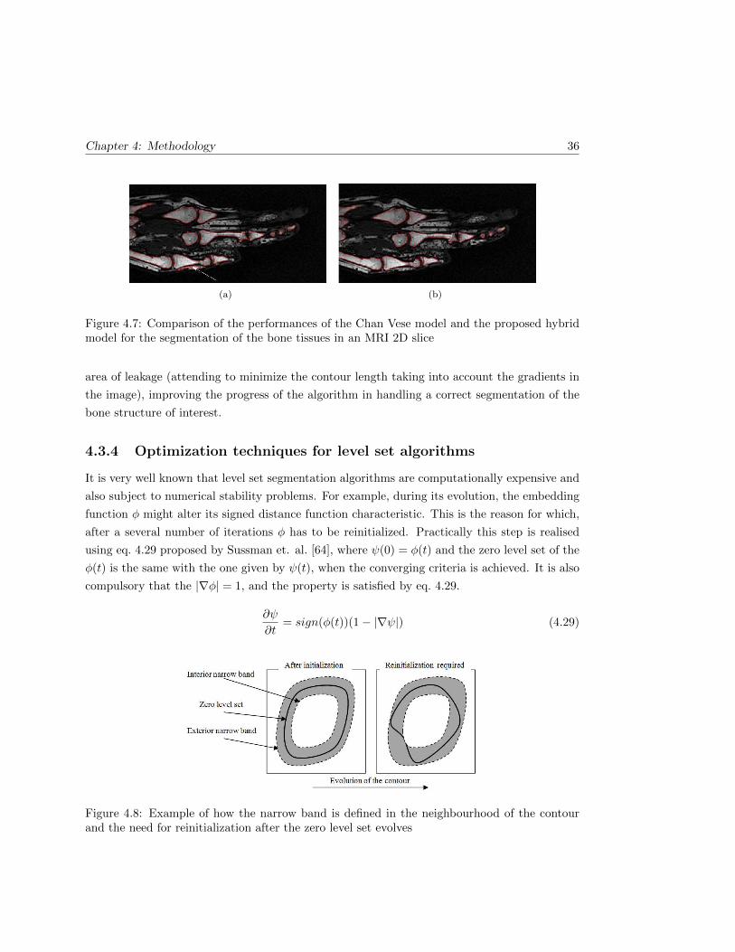
Chapter 4: Methodology 36
(a) (b)
Figure 4.7: Comparison of the performances of the Chan Vese model and the proposed hybridmodel for the segmentation of the bone tissues in an MRI 2D slice
area of leakage (attending to minimize the contour length taking into account the gradients in
the image), improving the progress of the algorithm in handling a correct segmentation of the
bone structure of interest.
4.3.4 Optimization techniques for level set algorithms
It is very well known that level set segmentation algorithms are computationally expensive and
also subject to numerical stability problems. For example, during its evolution, the embedding
function φ might alter its signed distance function characteristic. This is the reason for which,
after a several number of iterations φ has to be reinitialized. Practically this step is realised
using eq. 4.29 proposed by Sussman et. al. [64], where ψ(0) = φ(t) and the zero level set of the
φ(t) is the same with the one given by ψ(t), when the converging criteria is achieved. It is also
compulsory that the |∇φ| = 1, and the property is satisfied by eq. 4.29.
∂ψ
∂t= sign(φ(t))(1− |∇ψ|) (4.29)
Figure 4.8: Example of how the narrow band is defined in the neighbourhood of the contourand the need for reinitialization after the zero level set evolves
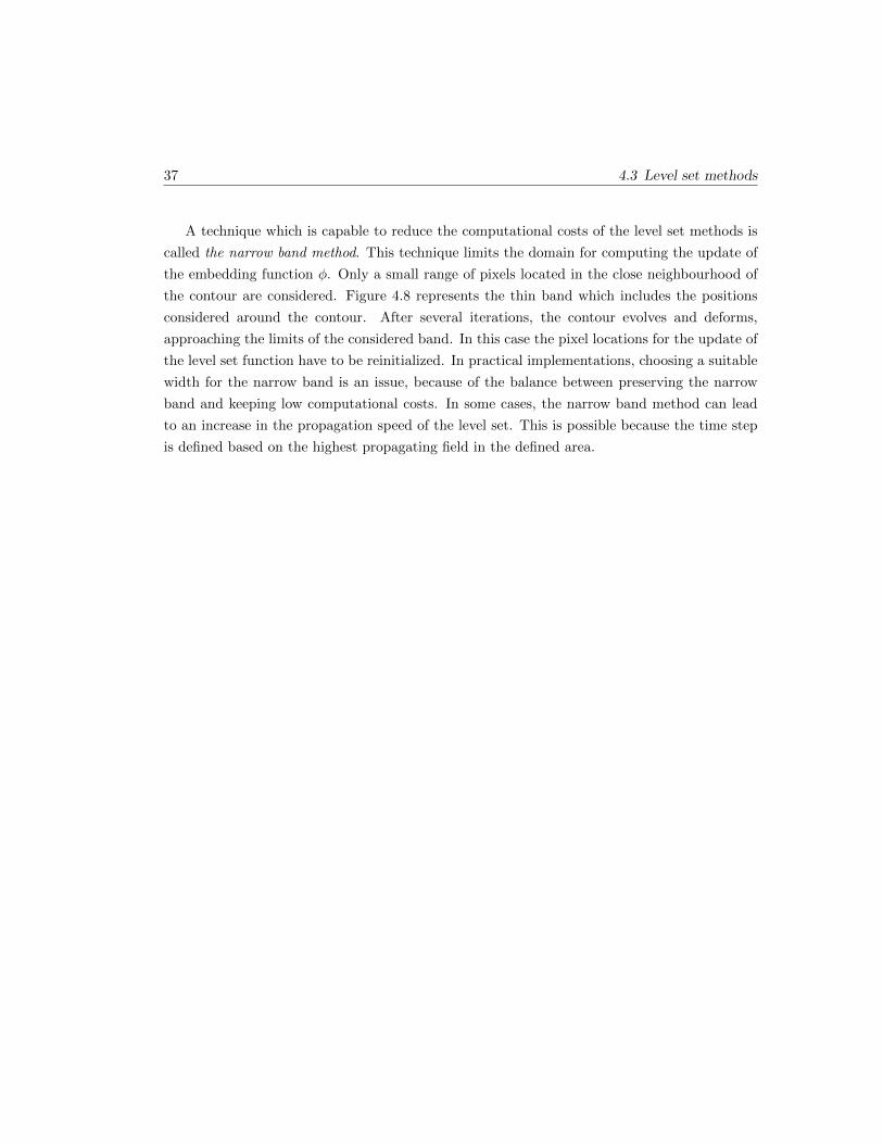
37 4.3 Level set methods
A technique which is capable to reduce the computational costs of the level set methods is
called the narrow band method. This technique limits the domain for computing the update of
the embedding function φ. Only a small range of pixels located in the close neighbourhood of
the contour are considered. Figure 4.8 represents the thin band which includes the positions
considered around the contour. After several iterations, the contour evolves and deforms,
approaching the limits of the considered band. In this case the pixel locations for the update of
the level set function have to be reinitialized. In practical implementations, choosing a suitable
width for the narrow band is an issue, because of the balance between preserving the narrow
band and keeping low computational costs. In some cases, the narrow band method can lead
to an increase in the propagation speed of the level set. This is possible because the time step
is defined based on the highest propagating field in the defined area.
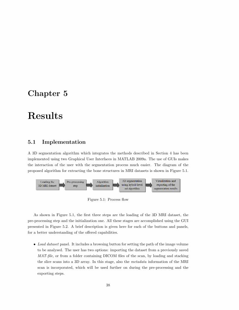
Chapter 5
Results
5.1 Implementation
A 3D segmentation algorithm which integrates the methods described in Section 4 has been
implemented using two Graphical User Interfaces in MATLAB 2009a. The use of GUIs makes
the interaction of the user with the segmentation process much easier. The diagram of the
proposed algorithm for extracting the bone structures in MRI datasets is shown in Figure 5.1.
Figure 5.1: Process flow
As shown in Figure 5.1, the first three steps are the loading of the 3D MRI dataset, the
pre-processing step and the initialization one. All these stages are accomplished using the GUI
presented in Figure 5.2. A brief description is given here for each of the buttons and panels,
for a better understanding of the offered capabilities.
• Load dataset panel. It includes a browsing button for setting the path of the image volume
to be analysed. The user has two options: importing the dataset from a previously saved
MAT-file, or from a folder containing DICOM files of the scan, by loading and stacking
the slice scans into a 3D array. In this stage, also the metadata information of the MRI
scan is incorporated, which will be used further on during the pre-processing and the
exporting steps.
38

39 5.1 Implementation
Figure 5.2: Graphical User Interface (GUI) for 3D MRI data loading, pre-processing and ini-tialization
• Pre-processing step panel. It implements the noise removal and edge enhancement pre-
processing phase using the anisotropic filtering technique developed in Section 4.1.2. As
explained, two parameters are required: the number of iterations the algorithm has to
run and the coefficient which controls the diffusion process.
• Type of initialization. In the initialization step the user has to select the starting regions
for the bone structures. The initialization for the final segmentation algorithm does not
need to be very accurate, but it has to provide only regions inside the structures to
be segmented, and not on their borders or outside them. The K-means approach (as
explained in Section 3.3) is based on the assumption that the 3D dataset can be clustered
in 3 classes: background, soft tissue and bone. After the K-means clustering technique
is run, the initialization 3D volume contains only the pixels considered as bone class. As
an alternative, the user can select to threshold the 3D volume. It is known that bone
structures usually have higher intensity gray levels than those of the surrounding tissues.
Therefore, after visual inspection, the user can select a threshold for binarizing the dataset
into bone and non-bone regions. In this case the single-threshold introduced in eq. 3.1 is
used.
• Volume analysis panel. Using the binary initialization 3D volume produced in the previous
step, having 1 for a bone voxel and 0 for a non-bone voxel, an algorithm for computing
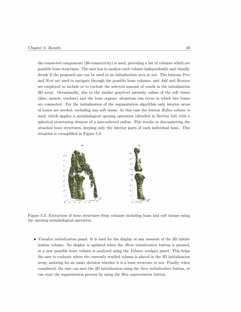
Chapter 5: Results 40
the connected components (26-connectivity) is used, providing a list of volumes which are
possible bone structures. The user has to analyse each volume independently and visually
decide if the proposed one can be used as an initialization area or not. The buttons Prev
and Next are used to navigate through the possible bone volumes, and Add and Remove
are employed to include or to exclude the selected amount of voxels in the initialization
3D array. Occasionally, due to the similar graylevel intensity values of the soft tissue
(skin, muscle, tendons) and the bone regions, situations can occur in which two bones
are connected. For the initialization of the segmentation algorithm only interior areas
of bones are needed, excluding any soft tissue. In this case the button Refine volume is
used, which applies a morphological opening operation (detailed in Section 3.6) with a
spherical structuring element of a user-selected radius. This results in disconnecting the
attached bone structures, keeping only the interior parts of each individual bone. This
situation is exemplified in Figure 5.3.
Figure 5.3: Extraction of bone structures from volumes including bone and soft tissues usingthe opening morphological operation
• Visualize initialization panel. It is used for the display at any moment of the 3D initial-
ization volume. Its display is updated when the Show initialization button is pressed,
or a new possible bone volume is analysed using the Volume analysis panel. This helps
the user to evaluate where the currently studied volume is placed in the 3D initialization
array, assisting for an easier decision whether it is a bone structure or not. Finally, when
considered, the user can save the 3D initialization using the Save initialization button, or
can start the segmentation process by using the Run segmentation button.
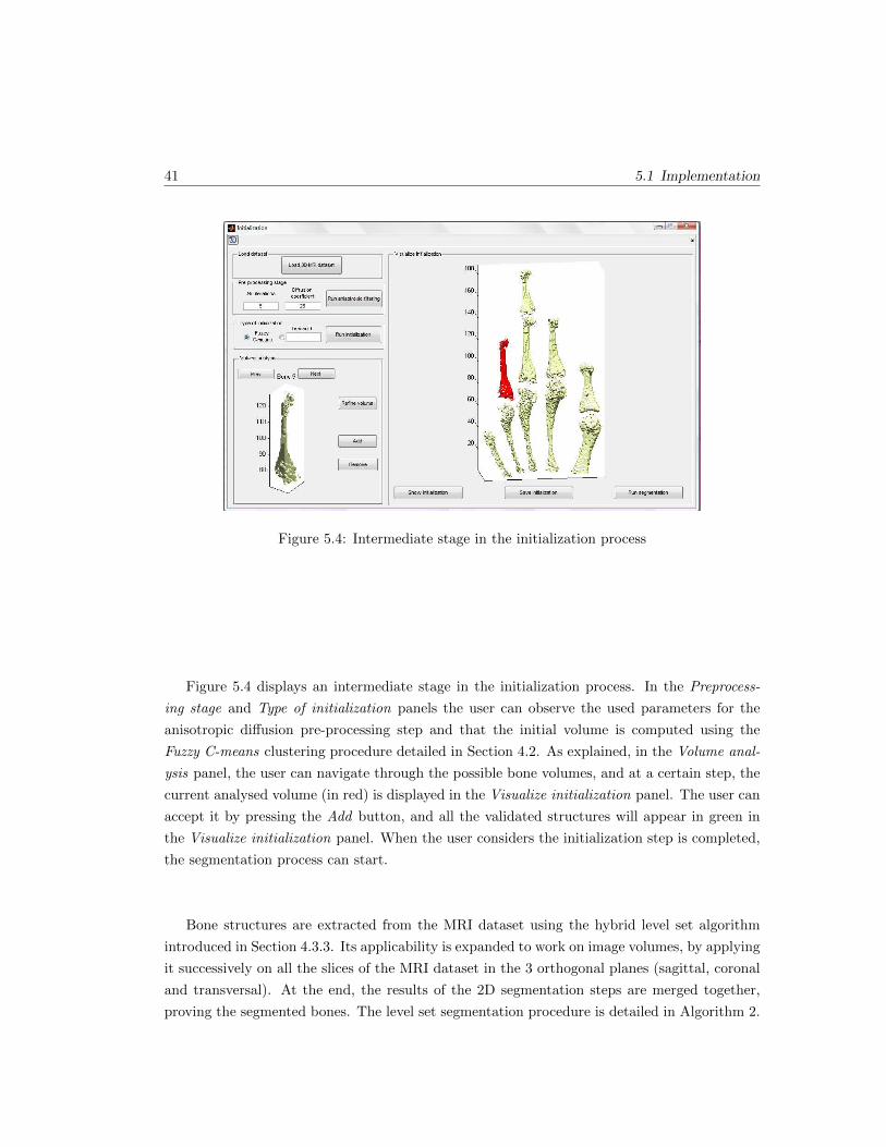
41 5.1 Implementation
Figure 5.4: Intermediate stage in the initialization process
Figure 5.4 displays an intermediate stage in the initialization process. In the Preprocess-
ing stage and Type of initialization panels the user can observe the used parameters for the
anisotropic diffusion pre-processing step and that the initial volume is computed using the
Fuzzy C-means clustering procedure detailed in Section 4.2. As explained, in the Volume anal-
ysis panel, the user can navigate through the possible bone volumes, and at a certain step, the
current analysed volume (in red) is displayed in the Visualize initialization panel. The user can
accept it by pressing the Add button, and all the validated structures will appear in green in
the Visualize initialization panel. When the user considers the initialization step is completed,
the segmentation process can start.
Bone structures are extracted from the MRI dataset using the hybrid level set algorithm
introduced in Section 4.3.3. Its applicability is expanded to work on image volumes, by applying
it successively on all the slices of the MRI dataset in the 3 orthogonal planes (sagittal, coronal
and transversal). At the end, the results of the 2D segmentation steps are merged together,
proving the segmented bones. The level set segmentation procedure is detailed in Algorithm 2.

Chapter 5: Results 42
Algorithm 2: Hybrid level set segmentation
1. Load the current 2D slice and the corresponding initialization.
2. Compute the initial embedding function φ, using a signed distance map (SDF) introduced
in eq. 4.29 and the initial mask which defines the bone regions.
3. Compute the mean values for the interior and exterior regions, as well as the variances,
and generate the edge-detector function.
4. Update the embedding function φk+1 = φk +∂φ
∂tdt, using eq. 4.27 for the computation of
∂φ
∂t.
5. Reinitialize the distance function (SDF) for numerical stability reasons.
6. Repeat steps 3 to 5 until the level set converges (no evolution over several steps).
(a) (b)
Figure 5.5: The result provided by the segmentation algorithm: (a) Initialization, (b) Finalsegmentation
The result of the 3D hybrid level set segmentation algorithm provides a 3D array, having
the same size of the MRI dataset, with values of 1 on voxels classified as part of a bone
structure and 0 otherwise. Figure 5.5 displays the resulting segmentation (Figure 5.5(b) having
as initialization the volume provided in Figure 5.5(a). It can be concluded that the convergence
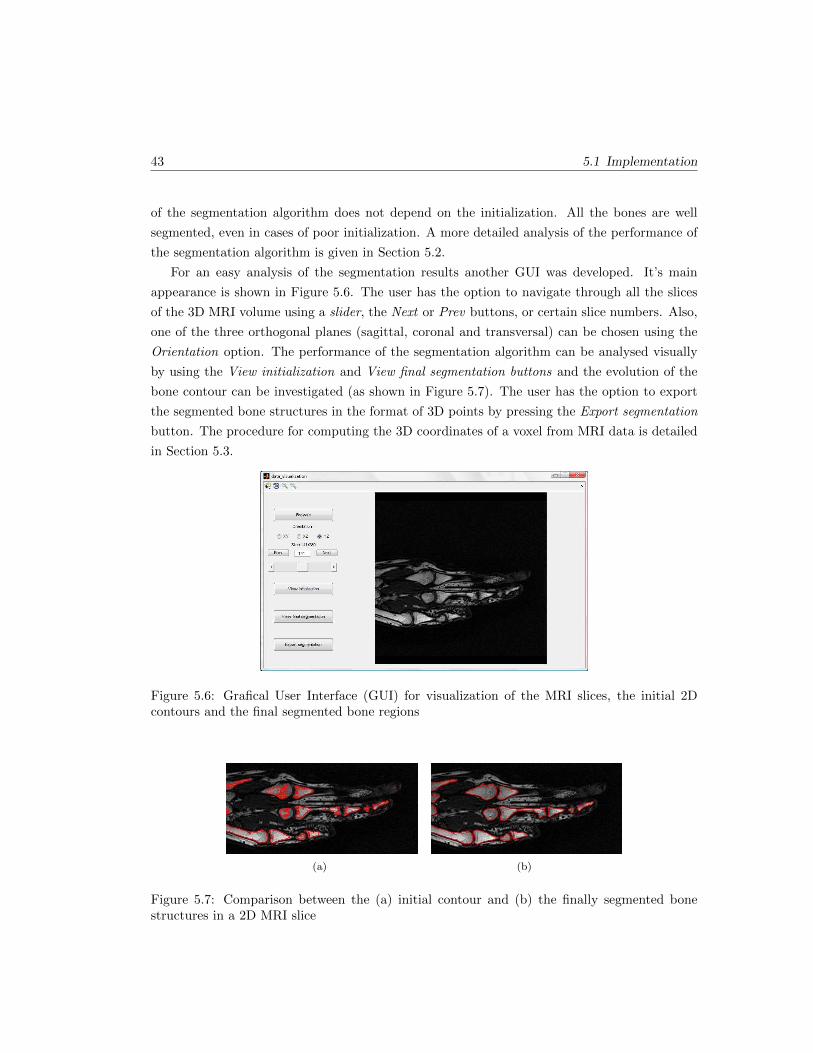
43 5.1 Implementation
of the segmentation algorithm does not depend on the initialization. All the bones are well
segmented, even in cases of poor initialization. A more detailed analysis of the performance of
the segmentation algorithm is given in Section 5.2.
For an easy analysis of the segmentation results another GUI was developed. It’s main
appearance is shown in Figure 5.6. The user has the option to navigate through all the slices
of the 3D MRI volume using a slider, the Next or Prev buttons, or certain slice numbers. Also,
one of the three orthogonal planes (sagittal, coronal and transversal) can be chosen using the
Orientation option. The performance of the segmentation algorithm can be analysed visually
by using the View initialization and View final segmentation buttons and the evolution of the
bone contour can be investigated (as shown in Figure 5.7). The user has the option to export
the segmented bone structures in the format of 3D points by pressing the Export segmentation
button. The procedure for computing the 3D coordinates of a voxel from MRI data is detailed
in Section 5.3.
Figure 5.6: Grafical User Interface (GUI) for visualization of the MRI slices, the initial 2Dcontours and the final segmented bone regions
(a) (b)
Figure 5.7: Comparison between the (a) initial contour and (b) the finally segmented bonestructures in a 2D MRI slice
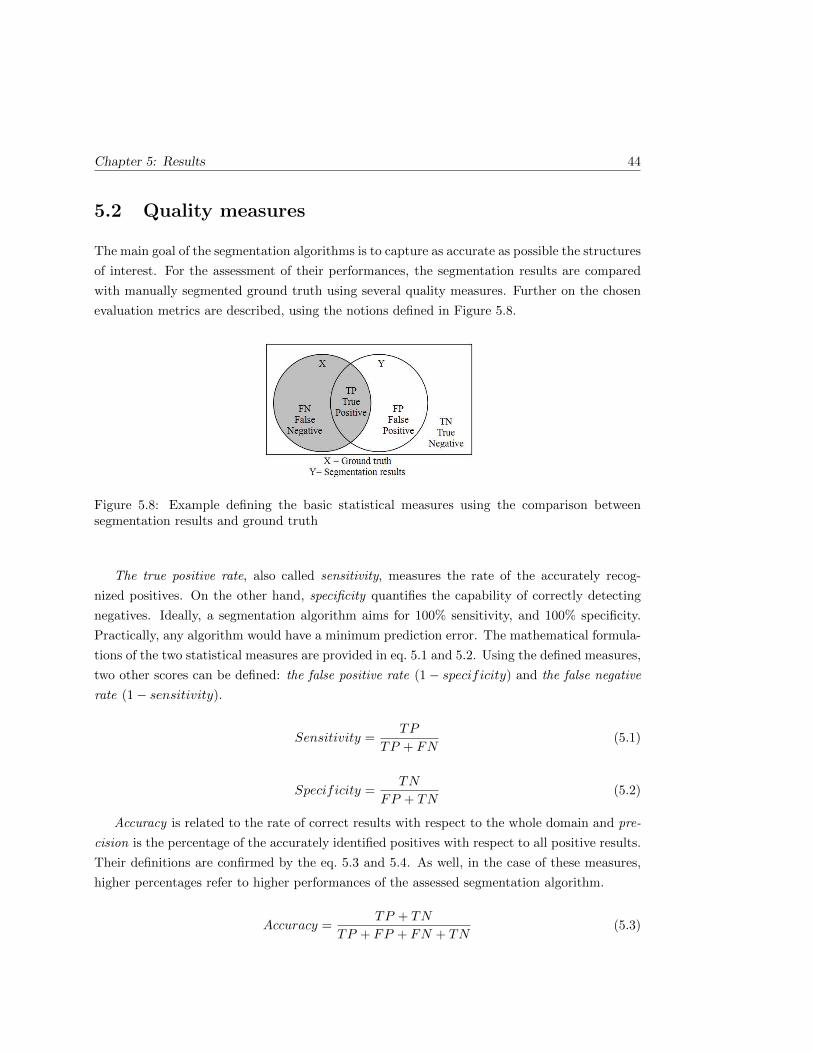
Chapter 5: Results 44
5.2 Quality measures
The main goal of the segmentation algorithms is to capture as accurate as possible the structures
of interest. For the assessment of their performances, the segmentation results are compared
with manually segmented ground truth using several quality measures. Further on the chosen
evaluation metrics are described, using the notions defined in Figure 5.8.
Figure 5.8: Example defining the basic statistical measures using the comparison betweensegmentation results and ground truth
The true positive rate, also called sensitivity, measures the rate of the accurately recog-
nized positives. On the other hand, specificity quantifies the capability of correctly detecting
negatives. Ideally, a segmentation algorithm aims for 100% sensitivity, and 100% specificity.
Practically, any algorithm would have a minimum prediction error. The mathematical formula-
tions of the two statistical measures are provided in eq. 5.1 and 5.2. Using the defined measures,
two other scores can be defined: the false positive rate (1− specificity) and the false negative
rate (1− sensitivity).
Sensitivity =TP
TP + FN(5.1)
Specificity =TN
FP + TN(5.2)
Accuracy is related to the rate of correct results with respect to the whole domain and pre-
cision is the percentage of the accurately identified positives with respect to all positive results.
Their definitions are confirmed by the eq. 5.3 and 5.4. As well, in the case of these measures,
higher percentages refer to higher performances of the assessed segmentation algorithm.
Accuracy =TP + TN
TP + FP + FN + TN(5.3)

45 5.2 Quality measures
Precision =TP
TP + FP(5.4)
The similarity between the ground truth and the segmentation results can be also computed
using the Dice coefficient and is defined as shown in eq. 5.5. A low value for the Dice coefficient
would suggest that there is low similarity between the ground truth and the outcome of the
segmentation algorithm, while a unity coefficient would denote a perfect segmentation.
Dice =2(X ∩ Y )
X + Y
=2TP
(TP + FP ) + (TP + FN)(5.5)
Having described in Figure 5.9 the names of the bones in the human hand, Table 5.1 provides
the quality measures of the 3D segmentation algorithm with respect to a manual segmentation
considered as the ground truth. The analysis of the segmentation measures in Table 5.1 confirms
the good performances of the segmentation algorithm. The high values of the quality measures
approve that the algorithm handles a very good segmentation of the bone structures in the
MRI datasets. The most relevant measures are the Sensitivity, Dice coefficient and Precision
which best describe how much of the ground truth regions are successfully segmented. The high
values for the Specificity and Accuracy are justified by the comparison of the segmentation of
a single bone volume with respect to the whole dataset volume.
Figure 5.9: Notations of the bones in the human hand
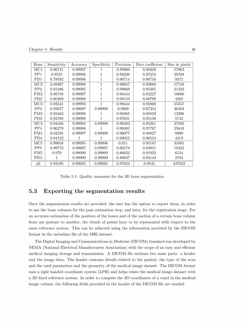
Chapter 5: Results 46
Bone Sensitivity Accuracy Specificity Precision Dice coefficient Size in pixelsMC1 0.96741 0.99997 1 0.99969 0.98329 57963PP1 0.9555 0.99998 1 0.99226 0.97353 29708PD1 0.78592 0.99996 1 0.96714 0.86716 9372MC2 0.88367 0.99988 1 0.99647 0.93668 57743PP2 0.91286 0.99995 1 0.99869 0.95385 31323PM2 0.86748 0.99997 1 0.98444 0.92227 10606PD2 0.80409 0.99998 1 0.99143 0.88799 4202MC3 0.92541 0.99993 1 0.99444 0.95868 55557PP3 0.95677 0.99997 0.99999 0.9909 0.97354 36383PM3 0.93463 0.99998 1 0.98305 0.95823 13396PD3 0.92768 0.99999 1 0.97631 0.95138 5742MC4 0.94166 0.99994 0.99998 0.96383 0.95261 37930PP4 0.96279 0.99998 1 0.99302 0.97767 25643PM4 0.82595 0.99997 0.99999 0.96077 0.88827 8999PD4 0.94122 1 1 0.99052 0.96524 4219MC5 0.99658 0.99995 0.99996 0.911 0.95187 31685PP5 0.99772 0.99997 0.99997 0.90574 0.94951 18322PM5 0.979 0.99999 0.99999 0.86632 0.91922 6134PD5 1 0.99999 0.99999 0.88937 0.94144 2784
all 0.93195 0.99935 0.99985 0.97824 0.9545 447832
Table 5.1: Quality measures for the 3D bone segmentation
5.3 Exporting the segmentation results
Once the segmentation results are provided, the user has the option to export them, in order
to use the bone volumes for the pose estimation step, and later, for the registration stage. For
an accurate estimation of the position of the bones and of the motion of a certain bone volume
from one posture to another, the clouds of points have to be represented with respect to the
same reference system. This can be achieved using the information provided by the DICOM
format in the metadata file of the MRI dataset.
The Digital Imaging and Communications in Medicine (DICOM) standard was developed by
NEMA (National Electrical Manufacturers Association) with the scope of an easy and efficient
medical imaging storage and transmission. A DICOM file encloses two main parts: a header
and the image data. The header contains details related to the patient, the type of the scan
and the used parameters and the geometry of the medical image dataset. The DICOM format
uses a right handed coordinate system (LPH) and helps relate the medical image dataset with
a 3D fixed reference system. In order to compute the 3D coordinates of a voxel in the medical
image volume, the following fields provided in the header of the DICOM file are needed:
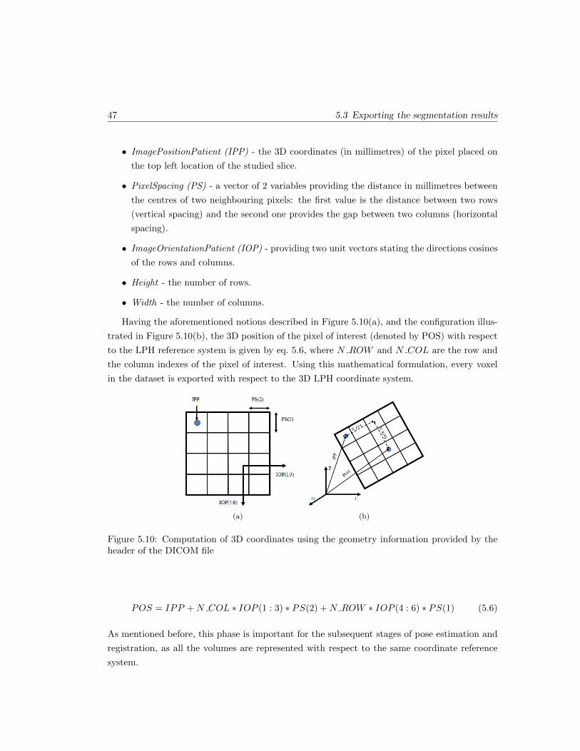
47 5.3 Exporting the segmentation results
• ImagePositionPatient (IPP) - the 3D coordinates (in millimetres) of the pixel placed on
the top left location of the studied slice.
• PixelSpacing (PS) - a vector of 2 variables providing the distance in millimetres between
the centres of two neighbouring pixels: the first value is the distance between two rows
(vertical spacing) and the second one provides the gap between two columns (horizontal
spacing).
• ImageOrientationPatient (IOP) - providing two unit vectors stating the directions cosines
of the rows and columns.
• Height - the number of rows.
• Width - the number of columns.
Having the aforementioned notions described in Figure 5.10(a), and the configuration illus-
trated in Figure 5.10(b), the 3D position of the pixel of interest (denoted by POS) with respect
to the LPH reference system is given by eq. 5.6, where N ROW and N COL are the row and
the column indexes of the pixel of interest. Using this mathematical formulation, every voxel
in the dataset is exported with respect to the 3D LPH coordinate system.
(a) (b)
Figure 5.10: Computation of 3D coordinates using the geometry information provided by theheader of the DICOM file
POS = IPP +N COL ∗ IOP (1 : 3) ∗ PS(2) +N ROW ∗ IOP (4 : 6) ∗ PS(1) (5.6)
As mentioned before, this phase is important for the subsequent stages of pose estimation and
registration, as all the volumes are represented with respect to the same coordinate reference
system.
Chapter 6
Conclusions
This chapter gives a short discussion on the achievements of this work, concluding and evalu-
ating the results and giving suggestions for further work to be undertaken.
6.1 Conclusions
In this thesis, an application is developed to solve the bone segmentation problem in 3D MR
images. The main purpose of developing a standalone application, which interacts with the
user for an accurate segmentation, has been accomplished.
In order to derive a precise kinematic model of the human hand, in vivo scans of different
postures have been obtained. Even though CT imaging would be suitable for this assignment,
it has been discarded because of radiation exposure. Therefore MRI imaging techniques have
been chosen, even though they are slower and provide lower resolutions. Consequently the
designed algorithm has to take into account the problems which might be encountered during
the segmentation process. Investigation for finding a suitable method which removes the noise
in the MRI scans has been conducted. Wavelet-based denoising techniques have been compared
with anisotropic filtering, and the last one has been chosen, as it is the most efficient in removing
the noise and preserving the features of interest for the segmentation algorithm.
A hybrid level set method has been used for the 3D segmentation of the bone structures. It
includes region-based and edge-information, in order to capture the bone contours in cases of
weak boundaries between the bone marrow and the cancellous bone. The approach also takes
into consideration the non-uniform intensity distribution in the bone structures. As level set
methods require initialization, a Fuzzy C-means clustering algorithm is used, considering that
the dataset comprises three main classes: background, soft tissues, bone.
48
49 6.2 Further work
The segmentation algorithm is tested on 50 postures of the hand, on 3 different subjects.
It proved to have high performance in extracting the bone postures and the results have been
compared with manual generated ground truth. Several quality measures have been applied,
providing an average sensitivity of 93% and a Dice similarity coefficient of 95%.
6.2 Further work
This work includes a comprehensive analysis of one of the main stages for hand kinematics
modelling using 3D MRI volumes. Further work can be undertaken to either improving the
segmentation algorithms which are required to extract very accurate the bone structures from
the medical image datasets, or to developing algorithms which would make the task of registering
two postures easier. Each of the approaches is detailed independently.
Related to the segmentation of each bone in each posture of the hand, several aspects can
be improved.
• Extension of the proposed algorithm to work directly on surfaces. This implies to use as
initialization a surface in the 3D volume and to apply the internal and external forces,
which produce the 3D contour evolution, on the mesh points which define the zero level set
of the surface. The main concern in this case is the memory use (avoid ”out of memory”
states) and the computational load, as the 3D MRI datasets are very large.
• Another enhancement of the application would refer to automatically initialize the level set
algorithm. As the algorithm requires for initialization only area inside the bone volumes,
this can be a very difficult task to achieve. In some cases the bone volumes can be easily
identified, based on their shape, but in other cases, as some volumes also include bone and
soft tissue, the method has to decide how to separate the two structures and to solely keep
the valid volumes. Moreover, due to intensity inhomogeneities, a bone can be divided in
several parts, so the shape information cannot be used for the decision.
• An additional suggestion refers to computation time improvement. As it is known that
level set methods are computationally expensive, an extension of the proposed algorithm
to fast level set techniques can be implemented.
Analysing the acquired MRI datasets of the hand in different postures, it can be concluded
that depending on the position and configuration of the hand and also on the MRI signal,
bones have different appearances, shape and gray level distributions. For deriving an accurate
kinematic model of the hand, precise registration of the bones in different postures is required
(which cannot be accomplished when the same bone has different shapes in 2 consecutive

Chapter 6: Conclusions 50
poses). This leads to an approach that carries out the segmentation and registration steps
simultaneously. this would require the segmentation of the bones in a single posture (obtaining
a representative shape for each structure), the creation of an atlas (expected shapes) and the
performance of the registration of the defined profiles in the rest of the scanned postures of the
hand.

Bibliography
[1] Hand. Britannica Encyclopaedia. http://www.britannica.com/EBchecked/media/101313/Bones-
of-the-hand-showing-the-carpal-bones-metacarpal-bones, 2011.
[2] G. B. Aboutanos, J. Nikanne, N. Watkins, and B. M. Dawan. Model creation and defor-
mation for the automatic segmentation of the brain in mr images. IEEE Transactions on
Biomedical Engineering, 46(11):1346–1356, 1999.
[3] S. Aja Fernandez, C. Alberola Lopez, and C.F. Westin. Noise and signal estimation in
magnitude mri and rician distributed images: A lmmse approach. 17(8):1383–1398, August
2008.
[4] Santiago Aja-Fernndez, Antonio Tristn-Vega, and Carlos Alberola-Lpez. Noise estimation
in single- and multiple-coil magnetic resonance data based on statistical models. Magnetic
Resonance Imaging, 27(10):1397–1409, 2009.
[5] N. C. Andreasen, R. Rajarethinam, T. Cizadlo, S. Arndt, V. W. 2nd Swayze, L. A. Flash-
man, D. S. O’Leary, J. C. Ehrhardt, and W. T. Yuh. Automatic atlas-based volume
estimation of human brain regions from MR images. Journal of Computer Assisted To-
mography, 20(1):98–106, February 1996. PMID: 8576490.
[6] M. S. Atkins and B. T. Mackiewich. Handbook of medical imaging. chapter Fully auto-
mated hybrid segmentation of the brain, pages 171–183. Academic Press, Inc., Orlando,
FL, USA, 2000.
[7] K. T. Bae, M. L. Giger, C. T. Chen, and C. E. Jr Kahn. Automatic segmentation of liver
structure in CT images. Medical Physics, 20(1):71–78, February 1993. PMID: 8455515.
[8] J. C. Bezdek, L. O. Hall, and L. P. Clarke. Review of MR image segmentation techniques
using pattern recognition. Medical Physics, 20(4):1033–1048, August 1993. PMID: 8413011.
51
BIBLIOGRAPHY 52
[9] A. Bosnjak, G. Montilla, R. Villegas, and I. Jara. 3d segmentation with an application
of level set-method using mri volumes for image guided surgery. Conference Proceedings
of the International Conference of IEEE Engineering in Medicine and Biology Society,
2007:5263–5266.
[10] M. E. Brummer, R. M. Mersereau, R. L. Eisner, and R. R. J. Lewine. Automatic detection
of brain contours in MRI data sets. IEEE Transactions on Medical Imaging, 12(2):153–166,
1993.
[11] A. J. Burghardt, G. J. Kazakia, and S. Majumdar. A local adaptive threshold strategy for
high resolution peripheral quantitative computed tomography of trabecular bone. Annals
of Biomedical Engineering, 35(10):1678–1686, 2007.
[12] V. Caselles, R. Kimmel, and G. Sapiro. Geodesic active contours. International Journal
of Computer Vision, 22:61–79, 1995.
[13] T. F. Chan and L. A. Vese. Active contours without edges. IEEE Transactions on Image
Processing, 10:266–277, 2001.
[14] S. Chen and D. Zhang. Robust image segmentation using FCM with spatial constraints
based on new kernel-induced distance measure. Systems, Man, and Cybernetics, Part B:
Cybernetics, IEEE Transactions on, 34(4):1907–1916, August 2004.
[15] G. E. Christensen, S. C. Joshi, and M. I. Miller. Volumetric transformation of brain
anatomy. IEEE Transactions on Medical Imaging, 16:864–877, 1997.
[16] G. B. Coleman and H. C. Andrews. Image segmentation by clustering. Proceedings of the
IEEE, 67(5):773–785, 1979.
[17] L. Collins, C. J. Holmes, T. M. Peters, and A. C. Evans. Automatic 3-D model-based
neuroanatomical segmentation. Human Brain Mapping, 3(3):190–208, 1995.
[18] C. Davatzikos. Spatial normalization of 3d brain images using deformable models. Journal
of Computer Assisted Tomography, 20:656–665, 1996.
[19] B. Dogdas, D. Shattuck, and R. M. Leahy. Segmentation of skull in 3d human mr images
using mathematical morphology.
[20] D. L. Donoho. De-noising by soft-thresholding. IEEE Transactions on Information Theory,
41:613–627, 1995.
[21] M. Droske, B. Meyer, M. Rumpf, and K. Schaller. An adaptive level set method for medical
image segmentation, 2001.
53 BIBLIOGRAPHY
[22] A. A. Farag, H. Hassan, R. Falk, and S. G. Hushek. 3d volume segmentation of mra data
sets using level sets.
[23] Y. Ge, J. M. Fitzpatrick, B. M. Dawant, J. Bao, R. M. Kessler, and R. A. Margolin.
Accurate localization of cortical convolutions in MR brain images. IEEE Transactions on
Medical Imaging, 15(4):418–428, 1996. PMID: 18215924.
[24] G. Gerig, O. Kubler, R. Kikinis, and F. A. Jolesz. Nonlinear anisotropic filtering of MRI
data, 1992.
[25] A. F. Goldszal, C. Davatzikos, D. L. Pham, M. X. Yan, R. N. Bryan, and S. M. Resnick.
An image-processing system for qualitative and quantitative volumetric analysis of brain
images. Journal of Computer Assisted Tomography, 22(5):827–837, October 1998. PMID:
9754125.
[26] V. Grau, A. U. J. Mewes, M. Alcaniz, R. Kikinis, and S. K. Warfield. Improved watershed
transform for medical image segmentation using prior information. Medical Imaging, IEEE
Transactions on, 23(4):447–458, April 2004.
[27] R. M. Haralick and L. G. Shapiro. Image segmentation techniques. Computer Vision,
Graphics, and Image Processing, 29(1):100–132, January 1985.
[28] K. Held, E. R. Kops, B.J. Krause, W. M. 3rd Wells, and R. Kikinis. Markov random field
segmentation of brain MR images. IEEE Transactions on Medical Imaging, 16(6):878–886,
December 1997. PMID: 9533587.
[29] Y. Jiang. X-ray bone fracture subtraction using geodesic active contour and mathematical
morphology operations. In CARS, pages 226–231, 2003.
[30] G. Kaiser. A Friendly Guide to Wavelets. Birkhauser, August 1994.
[31] M. Kass, A. Witkin, and D. Terzopoulos. Snakes: Active contour models. INTERNA-
TIONAL JOURNAL OF COMPUTER VISION, 1(4):321–331, 1988.
[32] R. Khayati, M. Vafadust, F. Towhidkhah, and M. Nabavi. Fully automatic segmentation
of multiple sclerosis lesions in brain mr flair images using adaptive mixtures method and
markov random field model. Comput. Biol. Med., 38:379–390, March 2008.
[33] J. Kittler, J. Illingworth, and J. Fglein. Threshold selection based on a simple image
statistic. Computer Vision, Graphics, and Image Processing, 30(2):125–147, May 1985.
[34] G. Kom, A. Tiedeu, and M. Kom. Automated detection of masses in mammograms by
local adaptive thresholding. Computers in Biology and Medicine, 37(1):37–48, 2007.
BIBLIOGRAPHY 54
[35] J. Kratky and J. Kybic. Three-dimensional segmentation of bones from ct and mri using
fast level sets. Proceedings of SPIE, 6914(1):691447–691447–10, 2008.
[36] T. Lei and W. Sewchand. Statistical approach to x-ray CT imaging and its applications
in image analysis. i. statistical analysis of x-ray CT imaging. Medical Imaging, IEEE
Transactions on, 11(1):53–61, March 1992.
[37] C. Li, R. Huang, Z. Ding, C. Gatenby, D. Metaxas, and J. Gore. A variational level
set approach to segmentation and bias correction of images with intensity inhomogene-
ity. In Proceedings of the 11th International Conference on Medical Image Computing and
Computer-Assisted Intervention, Part II, MICCAI ’08, pages 1083–1091, Berlin, Heidel-
berg, 2008. Springer-Verlag.
[38] H. Li, R. Deklerck, B. De Cuyper, A. Hermanus, E. Nyssen, and J. Cornelis. Object recog-
nition in brain CT-scans: knowledge-based fusion of data from multiple feature extractors.
IEEE Transactions on Medical Imaging, 14(2):212–229, 1995. PMID: 18215825.
[39] S. Z. Li. Markov random field models in computer vision. In Proceedings of the third
European conference on Computer Vision (Vol. II), pages 361–370, Secaucus, NJ, USA,
1994. Springer-Verlag New York, Inc.
[40] Z. Liang, J. R. MacFall, and D. P. Harrington. Parameter estimation and tissue segmen-
tation from multispectral MR images. IEEE Transactions on Medical Imaging, 13(3):441–
449, September 1994.
[41] L. M. Lorigo, O. D. Faugeras, W. E. L. Grimson, R. Keriven, and R. Kikinis. Segmentation
of bone in clinical knee mri using texture-based geodesic active contours. In Proceedings of
the First International Conference on Medical Image Computing and Computer-Assisted
Intervention, MICCAI ’98, pages 1195–1204, London, UK, 1998. Springer-Verlag.
[42] J. B. A. Maintz and M. A. Viergever. A survey of medical image registration. Medical
Image Analysis, 2(1):1–36, March 1998.
[43] J. F. Mangin, V. Frouin, I. Bloch, J. Regis, and J. Lopez-Krahe. From 3d magnetic
resonance images to structural representations of the cortex topography using topology
preserving deformations. J. Math. Imaging Vis., 5:297–318, December 1995.
[44] I. N. Manousakas, P. E. Undrill, G. G. Cameron, and T. W. Redpath. Split-and-merge
segmentation of magnetic resonance medical images: performance evaluation and exten-
sion to three dimensions. Computers and Biomedical Research, an International Journal,
31(6):393–412, December 1998. PMID: 9843626.
55 BIBLIOGRAPHY
[45] D. Nadadur and R. M. Haralick. Recursive binary dilation and erosion using digital line
structuring elements in arbitrary orientations. Image Processing, IEEE Transactions on,
9(5):749–759, May 2000.
[46] L. Najman and M. Schmitt. Geodesic saliency of watershed contours and hierarchical
segmentation. IEEE Transactions on Pattern Analysis and Machine Intelligence, 18:1163–
1173, 1996.
[47] R. D. Nowak. Wavelet-based rician noise removal for magnetic resonance imaging, 1998.
[48] S. Osher and N. Paragios. Geometric Level Set Methods in Imaging,Vision,and Graphics.
Springer-Verlag New York, Inc., Secaucus, NJ, USA, 2003.
[49] S. Osher and J. A. Sethian. Fronts propagating with curvature dependent speed: Al-
gorithms based on hamilton-jacobi formulations. JOURNAL OF COMPUTATIONAL
PHYSICS, 79(1):12–49, 1988.
[50] P. Perona and J. Malik. Scale-space and edge detection using anisotropic diffusion. IEEE
Trans. Pattern Anal. Mach. Intell., 12:629–639, July 1990.
[51] D. L. Pham and J. L. Prince. An adaptive fuzzy c-means algorithm for image segmentation
in the presence of intensity inhomogeneities. Pattern Recognition Letters, 20:57–68, 1998.
[52] D. L. Pham, C. Xu, and J. L. Prince. A survey of current methods in medical image
segmentation. In Annual Review of Biomedical Engineering, volume 2, pages 315–338.
2000.
[53] J. L. Prince, A. P. Dagher, C. Xu, and D. Pham. An automated technique for statistical
characterization of brain tissues in magnetic resonance imaging. 1996.
[54] Nair T. R. G. Rai, G. N. H. and. Gradient based seeded region grow method for ct
angiographic image segmentation. CoRR, abs/1001.3735, 2010.
[55] P. K. Sahoo, S. Soltani, A. K. C. Wong, and Y. C. Chen. A survey of thresholding
techniques. Computer Vision, Graphics, and Image Processing, 41:233260, February 1988.
ACM ID: 46079.
[56] N. Sang, H. Li, W. Peng, and T. Zhang. Knowledge-based adaptive thresholding segmen-
tation of digital subtraction angiography images. Image Vision Comput., 25:1263–1270,
August 2007.
BIBLIOGRAPHY 56
[57] A. Sarti, C. Corsi, E. Mazzini, and C. Lamberti. Maximum likelihood segmentation of
ultrasound images with rayleigh distribution. IEEE Transactions on Ultrasonics, Ferro-
electrics and Frequency Control, 52(6):947–960, 2005.
[58] J. Serra. Image Analysis and Mathematical Morphology. Academic Press, Inc., Orlando,
FL, USA, 1983.
[59] L. Shapiro and G. Stockman. Computer Vision. Prentice Hall, January 2001.
[60] J. Sijbers, D. H. J. Poot, A. J. den Dekker, and W. Pintjens. Automatic estimation of
the noise variance from the histogram of a magnetic resonance image. Physics in Medicine
and Biology, 52(5):1335–1348, February 2007.
[61] G. Stillfried, U. Hillenbrand, M. Settles, and P. van der Smagt. MRI based skeletal hand
movement model. Springer Tracts on Advanced Robotics, 2011.
[62] G. Stillfried and P. van der Smagt. Movement model of a human hand based on mag-
netic resonance imaging (MRI). In 1st International Conference on Applied Bionics and
Biomechanics (ICABB) 2010, October 2010.
[63] M. Straka, A. La Cruz, A. Kochl, M. Sramek, M. E. Groller, and D. Fleischmann. 3D
watershed transform combined with a probabilistic atlas for medical image segmentation,
2003.
[64] M. Sussman, P. Smereka, and S. Osher. A level set approach for computing solutions to
incompressible two-phase flow. J. Comput. Phys., 114:146–159, September 1994.
[65] P. M. Thompson and A. W. Toga. Detection, visualization and animation of abnormal
anatomic structure with a deformable probabilistic brain atlas based on random vector field
transformations. Medical Image Analysis, 1(4):271–294, September 1997. PMID: 9873911.
[66] H. Tian, T. Srikanthan, and K. V. Asari. Automatic segmentation algorithm for the
extraction of lumen region and boundary from endoscopic images. Medical & Biological
Engineering & Computing, 39(1):8–14, 2001.
[67] J. K. Udupa and S. Samarasekera. Fuzzy connectedness and object definition: Theory, al-
gorithms, and applications in image segmentation. Graphical Models and Image Processing,
58(3):246–261, May 1996.
[68] H. A. Vrooman. kNN-based multi-spectral MRI brain tissue classification: manual training
versus automated atlas-based training. In Proceedings of SPIE, pages 61443L–61443L–9,
San Diego, CA, USA, 2006.
57 BIBLIOGRAPHY
[69] J. Wang, J. Kong, Y. Lu, M. Qi, and B. Zhang. A modified FCM algorithm for MRI
brain image segmentation using both local and non-local spatial constraints. Computerized
Medical Imaging and Graphics: The Official Journal of the Computerized Medical Imaging
Society, 32(8):685–698, December 2008. PMID: 18818051.
[70] W. M. Wells, W. L. Grimson, R. Kikinis, and F. A. Jolesz. Adaptive segmentation of MRI
data. IEEE Transactions on Medical Imaging, 15(4):429–442, 1996. PMID: 18215925.
[71] C. F. Westin, L. M. Lorigo, O. D. Faugeras, W. E. L. Grimson, S. Dawson, A. Norbash,
and R. Kikinis. Segmentation by adaptive geodesic active contours. In A. M. DiGioia and
S. Delp, editors, Proceedings of MICCAI 2000, Third International Conference on Med-
ical Image Computing and Computer-Assisted Intervention, pages 266–275, Pittsburgh,
October 11-14 2000.
[72] A. P. Witkin. Scale-space filtering. In IJCAI, pages 1019–1022, 1983.
[73] C. Xu and J. L. Prince. Snakes, shapes, and gradient vector flow. IEEE TRANSACTIONS
ON IMAGE PROCESSING, 7(3):359–369, 1998.
[74] M. S. Yang and C. F. Su. On parameter estimation for normal mixtures based on fuzzy
clustering algorithms. Fuzzy Sets Syst., 68:13–28, November 1994.
[75] L. A. Zadeh. Fuzzy sets as a basis for a theory of possibility. Fuzzy Sets and Systems,
1(1):3–28, January 1978.
[76] J. Zhang, C. H. Yan, C. K. Chui, and S. H. Ong. Fast segmentation of bone in CT images
using 3D adaptive thresholding. Computers in Biology and Medicine, 40(2):231–236, 2010.
[77] Y. Zhang, B. J. Matuszewski, L. K. Shark, and C. J. Moore. Medical image segmentation
using new hybrid level-set method. In Proceedings of the 2008 Fifth International Con-
ference BioMedical Visualization: Information Visualization in Medical and Biomedical
Informatics, pages 71–76, Washington, DC, USA, 2008. IEEE Computer Society.
[78] A. P. Zijdenbos and B. M. Dawant. Brain segmentation and white matter lesion detection
in MR images. Critical Reviews in Biomedical Engineering, 22(5-6):401–465, 1994. PMID:
8631195.


![al. et magnetic resonance imaging segmentation ... · which affect the effectiveness of the segmentation methods. Fuzzy C-means method proposed by Dunn [2] is one of the most widely](https://static.fdocuments.us/doc/165x107/5e764eb9b5799e0f2317c4d0/al-et-magnetic-resonance-imaging-segmentation-which-affect-the-effectiveness.jpg)


![arXiv:1902.01977v1 [eess.IV] 5 Feb 2019Technical Considerations for Semantic Segmentation in MRI using Convolutional Neural Networks Submitted to Magnetic Resonance in Medicine Arjun](https://static.fdocuments.us/doc/165x107/5f32e055f64e0d407d43d2fa/arxiv190201977v1-eessiv-5-feb-2019-technical-considerations-for-semantic-segmentation.jpg)