Section 5: Forecast Evaluation and Skill Scores - · PDF fileSection 5: Forecast Evaluation...

Analysis of Climate and Weather Data | Forecast Evaluation and Skill Scores | HS 2013 | christoph.frei [at] meteoswiss.ch 1

Section 5: Forecast Evaluation and Skill Scores


What is Forecast Evaluation ? •  Assessing the quality / error structure of forecasts by

comparison to independent observations

Input / Conditions

Model

Forecast: Statement

about Reality

Reality / Observations

Skill scores: Measures of forecast quality


“Forecasts” •  Weather Forecast

How accurate are temperature forecasts one day ahead?

•  Simulations of Climate Reproduce the distribution of mean summer precipitation in Europe?

•  Spatial analysis Estimate precipitation at a non-instrumented site from observations in the neighbourhood?

•  Remote sensing, …

Räisänen et al. 2004

Obs Model

www.meteoswiss.ch


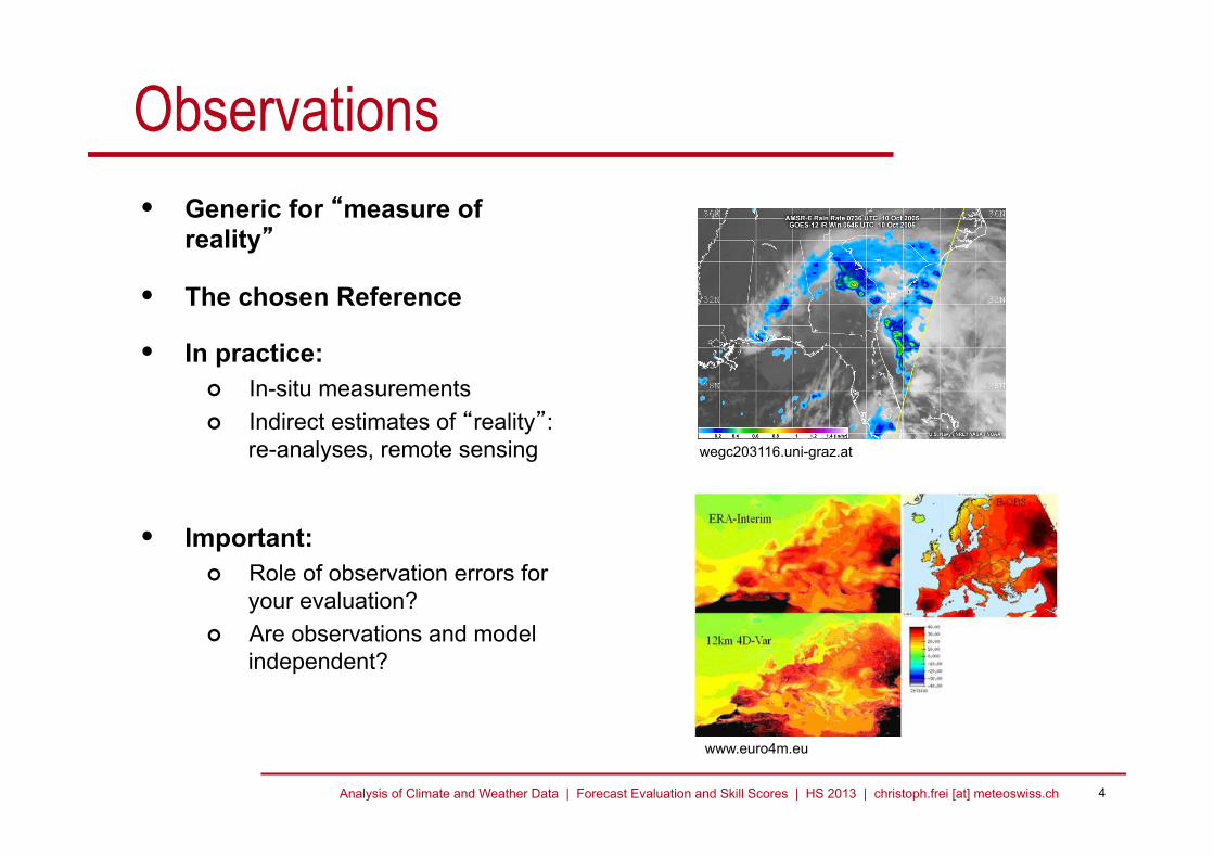
Observations •  Generic for “measure of

reality”

•  The chosen Reference

•  In practice:   In-situ measurements   Indirect estimates of “reality”:

re-analyses, remote sensing

•  Important:   Role of observation errors for

your evaluation?   Are observations and model

independent?

wegc203116.uni-graz.at

www.euro4m.eu


Why Forecast Evaluation? •  Learn how to properly use / interpret forecast

  E.g. the issuing of a public flood warning depends on the frequency with which the forecast produces false alarms

•  Learn how and where to improve forecast   E.g. by comparison of forecast quality for different model parametrizations

•  Justify investments made into models, instruments   E.g. launching of new weather satellites depends on the expected

improvement of weather forecasts (pay-back on investment)


ECMWF MR-Forecast Anomaly correlation of 500 hPa Geopotential

ECMWF 2012


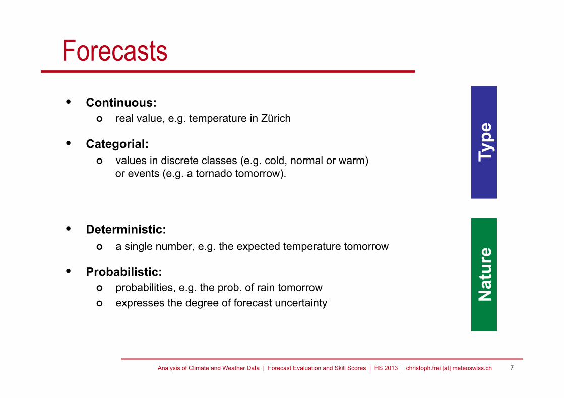
Forecasts •  Continuous:

  real value, e.g. temperature in Zürich

•  Categorial:   values in discrete classes (e.g. cold, normal or warm)

or events (e.g. a tornado tomorrow).

•  Deterministic:   a single number, e.g. the expected temperature tomorrow

•  Probabilistic:   probabilities, e.g. the prob. of rain tomorrow   expresses the degree of forecast uncertainty

Type

N

atur

e


Outline •  Deterministic categorial forecasts

•  Deterministic continuous forecasts

•  Probability forecasts

•  Evaluation based on economic value

•  Material based on:   Wilks 2005, Chap 7, (von Storch & Zwiers 1999, Chap 18)   Richardson 2000, Wilks 2001   Web-Site of WWRP/WGNE WG Forecast Verification Research:

http://www.cawcr.gov.au/projects/verification/


Deterministic Categorial Forecasts



yes no

yes a

hits

b false alarms

a+b

yes fcsts

no c

misses

d correct rejects

c+d no fcsts

a+c yes obs

b+d no obs

N total fcsts

Contingency Table •  Binary Forecasts

  Y = {yes, no}, e.g. events: tomorrow it will (will not) rain   simplest categorial case

•  Contingency Table   Distribution (Y,O) Observation

Fore

cast

Marginal of Obs

Mar

gina

l of F

cst

d

a c

b

obs. evts

fcst. evts


Finley Tornado Forecasts 1884

yes no

yes 28 72 100

no 23 2680 2703

51 2752 2803

Tornados Observed

Torn

ados

fore

cast

ed

U.S. Army forecasts of tornado occurrence east of the Rockies, based on synoptic information

www.photolib.noaa.gov

Galway 1985


Simple Scores •  Bias score:

  B = 1 unbiased, B < 1 underforecast, B > 1 overforecast   depends on marginals only, does not measure ‘correspondence’

•  Probability of detection (hit rate):

  Fraction of all observed events correctly forecasted   0 ≤ POD ≤ 1, best score: POD = 1, best score ≠ perfect fcst   Focus on events. No penalty for false alarms.

d

a

c

b

obs

fcst

B = a+ ba+ c

=forecasted eventsobserved events

POD =a

a+ c=

hitsobserved events


Simple Scores •  False alarm ratio:

  Fraction of forecasted events that were false alarms   0 ≤ FAR ≤ 1, best score: FAR = 0, best score ≠ perfect fcst

•  Probability of false detection (false alarm rate):

  Fraction of all non-events when forecast predicted an event   0 ≤ POFD ≤ 1, best score: POFD = 0 , best score ≠ perfect fc

FAR = ba+ b

=false alarms

forecasted events

POFD =b

b+ d=

false alarmsnon-events

d

a

c

b

obs

fcst


Simple Scores •  Accuracy (fraction correct):

  Fraction of all forecasts that were correct   0 ≤ ACC ≤ 1, best score: ACC = 1, best score = perfect fcst   Events and non-events treated symmetrically   For rare events the score is dominated by non-events   Finley tornado forecast:

•  ACC = (28+2680)/2803 = 0.96 (!) •  But: POD = 28/51 = 0.54 and FAR = 0.72 (!)

ACC = a+ dN

=correct forecasts

all forecasts

d

a

c

b

obs

fcst


Simple Scores •  Threat score (Critical Success Index):

  Fraction of all forecasted or observed events that were correct   0 ≤ TS ≤ 1, best score: TS = 1, best score = perfect fcst   Asymmetric between events and non-events.

  Finley tornado forecast: •  TS = 28/(28+72+23) = 0.23

TS =CSI = aa+ b+ c

=hits

all forecasted or observed events

d

a

c

b

obs

fcst


Limitations of Simple Scores •  How large is a “good” score?

•  Best score not necessarily perfect forecast!

•  Hedging (“Playing”) a score:   Example: Modify Finley’s Forecast --> constant forecast

yes no

yes 28 0 72 0

no 23 51 2680 2752

Observed

Fore

cast

ed

Finley: ACC = 0.96 Constant: ACC = 0.98 (!)


Generic Form of a Skill Score

SS =A! ArefAperf ! Aref

A accuracy score, e.g. ACC or TS Aref accuracy of reference forecast, e.g. random Aperf accuracy of perfect forecast

SS = 1 perfect forecast SS > 0 skillful, better than reference SS < 0 less skillful than reference


Heidke Skill Score •  Generic Score with …

… ACC as A and random forecast as reference

•  Heidke Skill Score

Aperf =1A = a+ dN

!

"#

$

%&

Aref =a+ b( )N

!

"#

$

%&'

a+ c( )N

!

"#

$

%&+

d + c( )N

!

"#

$

%&'

d + b( )N

!

"#

$

%&

HSS = ad ! bca+ c( ) " c+ d( )+ a+ b( ) " b+ d( )( ) 2

!" < HSS #1, HSS # 0 no skill

d

a

c

b

obs

fcst


HSS for Finley Forecast •  HSS

  for Finley forecast: HSS=0.355   for constant forecast: HSS=0.0

  note, ACC is large even for random forecast:

•  HSS (generic form of skill scores) compensates for high random ACC, when events are very rare.

ACCrandom =28+ 722803

!

"#

$

%&'28+ 232803

!

"#

$

%&+

2680+ 232803

!

"#

$

%&'2680+ 722803

!

"#

$

%&= 0.947


Hanssen-Kuipers Discriminant •  Similar to HSS but unbiased ACC in denominator

•  Hanssen-Kuipers (also True Skill Statistic, Pierce Skill Score)

  –1 ≤ HK ≤ 1, HK ≤ 0 no skill,   for unbiased forecasts: HK = HSS   HK(Finley) = 0.523, HK(constant) = 0.0

HK =ad ! bc

a+ c( ) " b+ d( )= POD!POFD

SS = ACC ! ACCrandom

1! ACCunbiased random

ACCunbiased random =a+ c( )2 + b+ d( )2

N 2

d

a

c

b

obs

fcst


24h forecast 48h forecast

U. Damrath (DWD)

Example

LokalModell: Operational NWP model of DWD in 2002, dx = 7 km)

Evaluation for all grid points in

Germany for year 2002 Skill varies between seasons:

E.g. 24h fcst in summer is less accurate than 48h fcst in winter.

Hanssen-Kuipers Score (in %) for daily precipitation occurrence (P>1 mm)


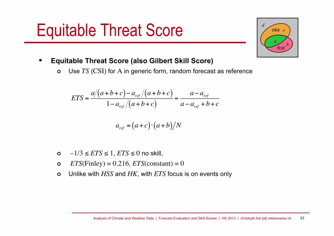
Equitable Threat Score •  Equitable Threat Score (also Gilbert Skill Score)

  Use TS (CSI) for A in generic form, random forecast as reference

  –1/3 ≤ ETS ≤ 1, ETS ≤ 0 no skill,   ETS(Finley) = 0.216, ETS(constant) = 0   Unlike with HSS and HK, with ETS focus is on events only

ETS =a a+ b+ c( )! aref a+ b+ c( )

1! aref a+ b+ c( )=

a! arefa! aref + b+ c

aref = a+ c( ) ! a+ b( ) N

d

a

c

b

obs

fcst


Skill Scores Differ … •  … in the relative importance of systematic and random errors

  E.g. artificially biasing a forecast decreases HK linearly but less than linearly for HSS

•  … in the relative role of events and non-events   ETS values only events <--> HSS, HK value both

•  … in their behaviour for rare events   Most skill scores tend to approach 0 for more and more rare events

•  There is no single best recommendation!


Uncertainty in Scores •  You’ve got 30 event forecasts.

You obtain HSS=0.2. Not too bad but …

•  … what is the probability that such a score is obtained by chance?


Further Remarks •  Sampling uncertainty

  Accuracy of skill scores decreases with sample size   Scores for forecasts of very rare events may be difficult to determine accurately.   Use resampling methods to quantify skill uncertainty.

•  Multi-category skill scores:   2x2 Table --> kxk Table   Extend classical scores to multi-category case.   E.g. ACC is sum of diagonal table elements divided by total forecasts.   Ordered multi-category case: introduce weights to penalize for elements more

far off the diagonal. (Gerrity 1992, see Wilks p. 274)


Deterministic Continuous Forecasts



Notation •  Sample, forecast-observation pairs (real valued)

•  Sample means

•  Sample variance

yi,oi{ }, i =1..N

y = 1N

yii! , o = 1

Noi

i!

sy2 =

1N

yi ! y( )i"

2, so

2 =1N

oi !o( )2i"


Example Data

•  24-h forecasts of T-max Oklahoma City

•  Comparison of:   NWS: Human forecast   NGM, LFM: Numerical model

forecasts with MOS   PER: Persistence forecast

•  Here   2 summers (1993/4, N=182)

Charles Doswell

Brooks & Doswell 1996


Simple Error Scores •  Bias (mean error, systematic error):

  additive, multiplicative

•  Mean absolute error:   Mean of absolute deviations from obs

•  Mean squared error (MSE), root MSE (RMSE):

  Sensitive to outliers, dominated by large deviations   Favors forecasts avoiding large deviations from the mean

Badd = y !o, Bmult = y o

MSE = 1N

yi !oi( )2 , RMSE = MSEi"

MAE = 1N

yi !oii"

0 !MAEMSERMSE

"

#$

%$

&

'$

($<)


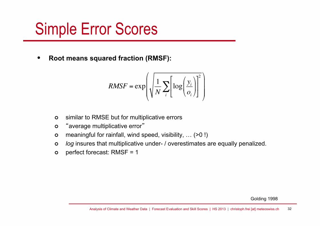
Simple Error Scores •  Root means squared fraction (RMSF):

  similar to RMSE but for multiplicative errors   “average multiplicative error”   meaningful for rainfall, wind speed, visibility, … (>0 !)   log insures that multiplicative under- / overestimates are equally penalized.   perfect forecast: RMSF = 1

RMSF = exp 1N

log yioi

!

"#

$

%&

'

()

*

+,

2

i-

!

"

###

$

%

&&&

Golding 1998


Correlation Skill Score •  Linear correlation coeff.

  –1 ≤ ρ ≤ 1, ρ = 1 best score   A measure of random error

(scatter around best fit)   Insensitive to biases and errors

in variance   ρ2: fraction of variance in obs

explained by “best” linear model

  ρ measures potential skill (see also later)

! =

1N

yi ! y( ) " oi !o( )i

N

#sy " so

Linear Regression:

Data: Brooks&Doswell 1996

1:1

best linear regression fit

NGM

ρ=0.88

oi = ! ! yi + a+"i


Conditional Bias •  Linear regression slope

  β = 1 best score   Deviations of β from 1 measure

conditional bias   β > 1: Large (small) values

tend to be under- (over-) estimated (unless compen-sated by absolute bias).

  β is a function of correlation and fraction of variances

! =sosy!"

Data: Brooks&Doswell 1996

1:1

best fit

NGM

ρ=0.88

β=1.23

Linear Regression:

oi = ! ! yi + a+"i


Decomposition of RMSE •  RMSE’ (debiased RMSE)

•  Geometric interpretation (cosine triangle theorem):

RMSE 2 = y !o( )2 + sy2 + so2 ! 2syso!

Taylor 2001

relative error in variance

degree of correspondence

!RMS "E 2

so2 =

RMSE 2 #B2

so2 =1+

sy2

so2 # 2

syso!

1 RMSE’ / so

sy / so

κ cos κ = ρ


Derivation

RMSE 2 =1N

yi !oi( )2" =1N

yi ! y( )! oi !o( )+ y !o( )( )2"

=1N

yi ! y( )! oi !o( )( )2" +

1N

y !o( )2"= sy

2 + so2 ! 2syso! +B

2

RMSE 2 !B2 = sy2 + so

2 ! 2syso!


Taylor Diagram •  Visualisation of forecast

performance by three related scores in one graph.

•  Ideal for:   Comparing several forecast

models,   Comparing to a reference

forecast   Comparing to several

observation datasets.   Assessing skill uncertainty e.g.

by ensembles.

Taylor 2001

RMSE’ / so sy / so

κ=arccos ρ

ρ


NWS: human forecaster NGM, LFM: numerical models PER: persistence forecast

Taylor Diagram •  Visualisation of forecast

performance by three related scores in one graph.

•  Ideal for:   Comparing several forecast

models,   Comparing to a reference

forecast   Comparing to several

observation datasets.   Assessing skill uncertainty e.g.

by ensembles.

Taylor 2001


Quiz •  How will the points change

with another obs. reference?

Indian Monsoon in global climate models

(AMIP Models) (from Taylor 2001)


Reduction of Variance

  also called Brier score or Nash-Sutcliffe Efficiency (Hydrology)   generic form of skill score with A=MSE and climatological forecast as

reference.   value range:   perfect forecast: SS = 1   climatology forecast: SS = 0   random forecast with same variance and mean like observations: SS = –1   sensitive to biases and errors in variance   Always: SS ≤ ρ2 (see later)   Oklahoma Temperature Forecast (NGM): SS = 0.607 (ρ2 = 0.77)

SS = MSE !MSEclim

MSEperfect !MSEclim

=1! MSEMSEclim

=1!

1N

yi !oi( )2"so2

!" < SS #1


Murphy-Epstein Decomposition •  Decomposition of SS (Reduction of Variance)

MSEMSEclim

=RMSE 2

so2 =

y !o( )2

so2 +1+

sy2

so2 ! 2

syso!

!!syso

"

#$

%

&'2

!!2

! "# $#

! SS =1" MSEMSEclim

= ! 2 " ! "syso

#

$%

&

'(

2

syso

""1( ))

*+

,

-.

2!"# $#

"y "o( )2

so2

linear correspondence “maximum explained variance”

penalty for absolute bias

penalty for conditional bias

Murphy & Epstein 1989

(see previously Taylor diagram)


Murphy-Epstein Decomposition •  Implications

  SS = ρ2 only for absolute and conditionally unbiased forecasts. I.e. ρ2 is a measure of potential skill.

  A non-perfect forcast (ρ2 < 1) can only be conditionally unbiased if sy < so , i.e. if variance is underestimated.

  Conditional bias can be minimized by setting sy/so = ρ, i.e. SS can be “played”!

  Among forecasts with the same ρ and the same absolute bias, SS (and RMSE) favors those with small conditional bias, i.e. too smooth forecasts.

  Forecasts with “good variance” are generally handicaped.


Oklahoma Temperatures

Model ρ2 (Conditional bias)^2

(Absolute bias)^2 SS

NWS 0.824 0.002 0.000 0.822

NGM 0.771 0.026 0.138 0.607

LFM 0.750 0.002 0.000 0.748

PER 0.382 0.141 0.000 0.241 persistence forecast

human forecast

β<1, because sy=so


Summary •  Correlation is a measure of potential skill only.

•  A thorough assessment of forecast quality requires consideration of several skill scores.

•  Frequently used scores favor smooth forecasts. It is difficult to demonstrate skill of high variability forecasts.

•  Use creative graphics (such as the Taylor diagram) to visualize several skill measures.

Section 5: Forecast Evaluation and Skill Scores - · PDF fileSection 5: Forecast Evaluation...

Documents

Transcript of Section 5: Forecast Evaluation and Skill Scores - · PDF fileSection 5: Forecast Evaluation...