- Bogotá - Colombia - Bogotá - Colombia - Bogotá - Colombia - Bogotá - Colombia - Bogotá - Colombia - Bogotá - Colombia - Bogotá - Colombia - Bogotá - Colombia - Bogotá -

On Forecast Evaluation∗

Wilmer Osvaldo Martınez-Rivera†

Manuel Dario Hernandez-Bejarano‡

Juan Manuel Julio-Roman§

Abstract

We propose to assess the performance of k forecast procedures by exploring thedistributions of forecast errors and error losses. We argue that non systematic forecasterrors minimize when their distributions are symmetric and unimodal, and that forecastaccuracy should be assessed through stochastic loss order rather than expected lossorder, which is the way it is customarily performed in previous work. Moreover, sinceforecast performance evaluation can be understood as a one way analysis of variance,we propose to explore loss distributions under two circumstances; when a strict (butunknown) joint stochastic order exists among the losses of all forecast alternatives,and when such order happens among subsets of alternative procedures. In spite of thefact that loss stochastic order is stronger than loss moment order, our proposals are atleast as powerful as competing tests, and are robust to the correlation, autocorrelationand heteroskedasticity settings they consider. In addition, since our proposals do notrequire samples of the same size, their scope is also wider, and provided that theytest the whole loss distribution instead of just loss moments, they can also be used tostudy forecast distributions as well. We illustrate the usefulness of our proposals byevaluating a set of real world forecasts.

Keywords: Forecast evaluation, Stochastic order, Multiple comparison.JEL: C53, C12, C14.

∗First Draft for comments, please do not circulate. We are grateful to Daniel Moreno-Cortes forhis careful proofreading. However, any remaining errors as well as the conclusions and opinions contained inthis paper are the sole responsibility of its authors and do not compromise BANCO DE LA REPUBLICA,its Board of Governors or Universidad Nacional de Colombia.

†wmartiri@banrep.gov.co, Specialized Professional, Statistics Division, Economic Research VP,

BANCO DE LA REPUBLICA, Bogota, Colombia.‡mhernabe@banrep.gov.co, Specialized Professional, Statistics Division, Economic Research VP,

BANCO DE LA REPUBLICA, Bogota, Colombia.§Corresponding author: jjulioro@banrep.gov.co, Senior Researcher, Research Unit, Technical Presi-

dency, BANCO DE LA REPUBLICA, and part time Associate Professor, Department of Statistics, Uni-versidad Nacional de Colombia, Bogota, Colombia.

1

Sobre la Evaluacion de Pronosticos§

Wilmer Osvaldo Martınez-Rivera1

Manuel Dario Hernandez-Bejarano2

Juan Manuel Julio-Roman3

Resumen

Proponemos evaluar el desempeno de k procedimientos de pronostico explorandolas distribuciones de los errores de pronostico y de sus perdidas. Argumentamos que loserrores no sistematicos de pronostico se minimizan cuando su distribucion es simetricay unimodal, y que la precision de los pronosticos debe evaluarse a traves del ordenestocastico de sus perdidas en vez del orden de las perdidas esperadas, que es como sepropone en trabajos anteriores. Adicionalmente, como la evaluacion de pronosticos sepuede entender como un analisis de varianza a una vıa, proponemos explorar las dis-tribuciones de las perdidas bajo dos circunstancias; cuando hay un orden estocasticoconjunto (desconocido) entre las perdidas de los k procedimientos, y cuando este ordenocurre en subconjutos de estos. A pesar de que el orden estocastico es mas fuerteque el orden de las perdidas esperadas, nuestras propuestas son tan potentes comolas competidoras ademas de ser robustas a las correlaciones, autocorrelaciones y het-erogeneidades consideradas para estas. De igual manera, como nuestras propuestasno requieren muestras del mismo tamano, su campo de aplicacion es mas amplio, ycomo exploran la distribucion de la perdida en vez de solo sus momentos, tambien sepueden utilizar para evaluar las distribuciones de pronostico de distintos procedimien-tos. Finalmente, ilustramos la utilidad de nuestras propuestas evaluando un conjuntode pronosticos de la vida real.

Palabras Clave: Evaluacion de pronosticos, Orden estocastico, Comparacionesmultiples.JEL: C53, C12, C14.

§Primera Version para comentarios, por favor no circular. Los autores agradecen a DanielMoreno Cortez por su cuidadosa prueba de lectura. Sin embargo, cualquier error que persista en esteescrito, asi como sus conclusiones y recomendaciones son responsabilidad exclusiva de sus autores y nocomprometen al BANCO DE LA REPUBLICA, su Junta Directiva o la Universidad Nacional de Colombia.

1wmartiri@banrep.gov.co, Profesional Especializado, Division de Estadıstica, Sub Gerencia de Estudios

Economicos, BANCO DE LA REPUBLICA, Bogota, Colombia.2mhernabe@banrep.gov.co, Profesional Especializado, Division de Estadıstica, Sub Gerencia de Estudios

Economicos, BANCO DE LA REPUBLICA, Bogota, Colombia.3Autor Corresponsal: Investigador Principal, Unidad de Investigaciones, Gerencia Tecnica, BANCO DE

LA REPUBLICA y Profesor Asociado, Departamento de Estadıstica, Universidad Nacional de Colombia.Bogota D. C., Colombia. e-mail:jjulioro@banrep.gov.co.

1 Introduction

Forecasting pervades all human endeavors particularly the design of policies in inflationtargeting central banks. In fact, under flexible forecast targeting the most importantoutputs of the central bank are the short to medium term inflation and economic activityforecasts, which arise from a great variety of sources like the central bank’s own suit ofmodels, surveys on external agents and experts, and from internal experts judgment. Theseforecasts are then comprised into the official ones which serve the board of governors asguide to design its policies. See Svensson (2007), for instance.

The summarization above is based on the assessment of the performance of relevantforecast alternatives, which can be based on two types of evaluation procedures; forecastinformation disagreement statistics like RMSE, MAE, MAPE, etc., which rank forecastperformance depending on the values these statistics assume, and formal forecast perfor-mance tests. The former ones are subject to criticism as they lack statistical significanceinterpretation, and therefore there is marked preference for the latter procedures. SeeHyndman and Athanasopoulos (2013) and Diebold and Mariano (1995), for example.

Two statistical tests stand out among the formal methodologies to determine theout of sample performance of a set of k ≥ 2 forecast procedures of an observable processXtt. Consider sample information consisting of k paired sets of size n, Xi1,Xi2, . . . ,Xinof out of sample forecast errors at a fixed horizon h, arising from i = 1, 2, . . . , k fore-cast procedures denoted M1,M2, . . . ,Mk,. Given a concave loss function L(·), and let-ting dt = [d1t, d2t, . . . , dk−1,t] be the loss difference process dit = L(Xit) − L(Xi+1,t),Mariano and Preve (2012), MP, propose to test the null of equal expected loss

H0 : E(dt) = 0 (1)

against the alternative of at least one difference

H1 : E(dt) 6= 0 (2)

using a Wald type statistic SMP = nd′Ω−1d, where Ω is an estimate of the asymptotic

(long run) variance covariance matrix of√n(d− µ

)and d = µ = E [dt]

4. Under the nulland the assumptions that the k ≥ 2 models producing the forecasts are arbitrary and dt is

stationary and has Wold representation, SMPD−→ χ2

(k) as n → ∞. These authors providethe conditions under which this asymptotic behavior is invariant to permutations of theprocedures, and also provide a modified test to correct SMP size in small samples, SMPc.

On the other hand, Giacomini and White (2006), GW, propose two tests; a con-ditional and an unconditional test for k = 2 only. The conditional test determines the

4Mariano and Preve (2012) test is a multivariate version of Diebold and Mariano (1995).In this setting it is customary to consider square, absolute, lin-lin and linex losses, among others.

2

more accurate forecast alternative for a specific horizon while the unconditional testsestablishes which of two alternatives was more accurate. The later test coincides withDiebold and Mariano (1995) test for k = 2. Under weaker assumptions than MP’s, the

unconditional test statistic tT,n,h =dT,n

σn/√nhas an asymptotic standard normal distribution

under H0 above, for k = 2, where T is the sample size used to forecast, dT,n = 1n

∑nt=1 dt,

and σ2n is the long run variance of√n(dt − E[dt]

).

These tests, MP and unconditional GW, have important advantages over previousmethodologies like the possibility of including heterogeneity, time series dependence, andstructural breaks within the forecast sample. However, they have important drawbacks aswell. First, these tests assess the relative performance of competing forecast alternativesthrough expected loss order only. By focusing on these figures many features of the fore-cast error and loss distributions of competing procedures are disregarded, which may leadto sub-optimal choices. Second, their tests statistics have asymptotic rather than exactdistributions under the null, which may lead to considerable size distortions in small sam-ples. And third, they have not been proved to be UMP, i.e. Uniformly Most Powerful.Therefore, room for improvement still remains.

We propose a two step methodology to assess the performance of a set of k ≥ 2forecast procedures by exploring the distribution of forecast errors and error losses. Inthe first step forecast alternatives are chosen to have desirable unconditional forecast errordistribution properties. In the second, the remaining procedures are ranked according tothe stochastic order of error losses. Under the assumption that there is a strict stochas-tic order among the loss functions of all k procedures, we propose to use the maximumJonckheere (1954) test statistic among all alternative order permutations to rank their jointperformance. However, if strict order happens only among subsets of alternatives, multiplecomparisons tests reveal their forecasting ability.

Using Jonckheere’s test for our procedures has several advantages over the afore-mentioned tests as well. First, Jonckheere’s test compares the distribution of error lossesinstead of expected losses. More specifically, the alternative of loss stochastic order isstronger than the alternative of expected loss order, being the former closer to “highly de-sirable” forecast behavior as it takes into account non systematic forecast error departuresfrom optimal forecasts. Second, Jonckheere’s test statistic has exact small sample distribu-tion under the null, which favors its use in many situations, e.g. when moving windows ofsmall size are analyzed as proposed by Fama and MacBeth (1973). Third, Jonckheere’s testis non parametric, that is no distributional sample assumption are imposed before hand.Fourth, if strict stochastic order exists only among subsets of the alternative procedures,the multiple comparisons test version provides their ranking as well. Furthermore, sinceJonckheere’s test works for non paired samples, its scope is wider as paired samples withmissing forecasts can be analyzed. And finally, since Jonckheere’s test probes the wholedistribution rather than just its moments, it may also be useful to assess the performance

3

Bayesian forecast error distributions.

We compare the power of the joint and multiple comparisons tests based on Jonckheere(1954)’s test with the power of the corresponding joint and multiple comparison versionsof Mariano and Preve (2012) test. We implemented two alternative simulation set ups toestimate the power function, the first follows closely Giacomini and White (2006) and thesecond is an adaptation of Mariano and Preve (2012).

Finally, we provide provide an illustration of the use of our tests in a real worldforecasting situation.

The rest of the paper is distributed in 4 sections apart from the introduction. Thesecond discusses the properties of well behaved forecast errors where we favor the use ofnon parametric tests with exact small sample distribution test statistics under the null. Inthe third we describe Jonckheere (1954)’s test and the procedures we propose. The fourthcontains the comparison of power functions and a real world illustration. The last containsthe conclusions and discussion.

2 What makes a good forecast procedure?

The properties of well behaved forecast are well known in the literature. A forecast alter-native is loss optimal if it minimizes the expected loss, i.e. the forecast risk, among forecastalternatives. Clearly, this kind of optimality does not necessarily lead to unbiased forecasts,which arise under squared loss, for instance. However, even in this case the distributionsof forecast errors and error losses might not necessarily be well behaved.

The case for forecast error distribution unimodality and symmetry relates to nonsystematic forecast errors. These types of errors occur when the frequency of forecast errorsin particular subsets of its support are unexpectedly large, e.g. under multi modality withwide gaps between the modes or under skewness. In the former case a higher than expectedfrequency of forecast errors will happen around each mode, and since the modes are wideapart a higher than expected frequency of large errors would arise. In the later case, ahigher than expected frequency of positive or negative forecast errors may also emerge.

These facts however, do not necessarily affect forecast unbiasedness, a systematicdistribution feature. In fact, strong non systematic departures from symmetry, for instance,may lead to forecast bias, but the implication the other way around is not warranted.Therefore, a clear distinction between systematic (e.g. unbiasedness) and non systematic(e.g. multi modality and lack of symmetry) forecast error distribution behaviors comes up,being the later more general and thus preferable than the former.

Under concave loss L(·) and forecast error distribution symmetry and unimodality,

4

the most common measure of forecast “accuracy” relates to expected loss minimization.Let Xi1,Xi2, . . . ,Xin be k size n sets of paired samples of forecast errors arising fromi = 1, 2, . . . , k forecast procedures denoted M1,M2, . . . ,Mk,. Forecast alternative Mi

is said to be “more accurate” than Mj 6= Mi if E[L(Xi,t)] < E[L(Xj,t)], which guidesthe hypotheses (1) and (2). It is also said that Mi is the “most accurate” among all kalternatives if it is “more accurate” than any other alternative.

However, loss optimality is not the only way to measure forecast “accuracy’. Infact, expected loss summarizes the behavior of the distribution of forecast errors throughits first moment only, which may lead, once again, to non-systematic loss deviations thatdepend on the shape of the distribution of error losses. Therefore, a stronger measure of“accuracy” can be obtained by comparing loss distributions as a whole.

We propose to test for loss stochastic order instead of expected losses. More formally,we say that Mi is “strictly more accurate” than Mj 6= Mi if L(Xi,t) ≺ L(Xj,t) where ≺means L(Xi,t) is of strictly smaller stochastic order than L(Xj,t), where “strict stochasticorder” is defined as

P [L(Xi,t) > x] < P [L(Xj,t) > x] ∀x ∈ R, (3)

P [L(Xi,t) > x] = 1 − Gi(x), and Gi(x) is the cumulative distribution function of theloss applied to the forecast errors of Mi. It is known that L(Xi,t) ≺ L(Xj,t) impliesE[L(Xi,t)] < E[L(Xj,t)] but the opposite implication is not warranted, and that (3) isequivalent to

Gj(x) < Gi(x) ∀x ∈ R (4)

For instance, if L(·) ≥ 0 and the bulk of the continuous densities gi and gj corre-sponding to Gi and Gj locate around a point X0 > 0, when gi is higher than gj aroundthe bulk, and the tail of gj is greater than the tail of gi, Mi has a higher frequency oflow losses than Mj , and Mj has a higher frequency of high losses than Mi. Therefore, ≺optimality of Mi with respect to Mj depends on the relative frequency of losses on subsetsof the support of L, in sharp contrast with the comparison of expected losses, which aresystematic features of loss distributions5.

Summarizing, we argue that the behavior of forecasts should not only be evaluatedthrough the comparison of systematic features of forecast error distributions (e.g. unbi-asedness) and expected error losses (e.g. expected losses), but through the comparisonof non systematic distributional features. This way, forecast comparison has to do with

5The statistical term “stochastic order” is known to labor economists as first order “stochastic dom-inance” who apply it to welfare comparison among populations as in Davidson (2008). In this context,several tests for first and higher order, i.e. restricted, stochastic dominance have been developed, whichhave not been considered in this work since their test statistics have asymptotic rather than exact smallsample known distributions under the null. See Davidson and Duclos (2013), for instance.

5

relative frequencies of forecast errors and error losses on subsets of their correspondingsupports rather than on systematic distributional features like moments. Therefore, nonsystematic features like unimodality, symmetry and loss stochastic order play a key role inforecast evaluation.

Testing the unconditional distribution of forecast errors: In order to test for thedesired non systematic behavior of forecast error distributions discussed in 2, availabletest for distribution symmetry, unimodality and (under square loss) zero location werechosen. For these tasks we prefer non-parametric exact small sample distribution teststatistics whenever they are available as they may have superior properties than parametricor asymptotic tests. Our choices are as follows.

1. Mira (2010) proposed a test to detect density lack of symmetry about an unknownmeasure of location, µ. Under the assumption that X1,X2, . . . ,Xn is an i.i.d. samplefrom a population with c.d.f. F (x) = F0(x− µ), the null H0 : F0(x) = 1−F0(−x) forall x ∈ R is rejected when |γ1(Fn)| ≥ an

n1/2Sc(γ1, Fn), where γ1 = 2(X2−Xs:n), X2 andXs:n are the sample mean and median, respectively, an −→ z1−α/2 as n −→ ∞ withz1−α/2 being the 1−α percentile of the standard normal distribution, and S2

c (γ1, Fn)being a weakly consistent estimate of the asymptotic variance of γ1.

2. In turn, Hartigan and Hartigan (1985) dip test seems to be one of the few optionsto test for distribution unimodality. This test measures multimodality in a sampleby calculating the maximum difference between the empirical distribution functionand a unimodal distribution function that minimizes this maximum difference. Thismaximum difference helps test the null of unimodality against multi modality.

3. Under square loss, optimal forecast error distribution should be located around zero,and therefore Wilcoxon (1945) one sample zero location (mean/median) test, H0 :µ = 0, under random sampling might be used. The null is rejected when the signedrank sum statistic W ≥ w1−α/2,n, where w1−α/2 is the 1−α/2 percentile of Wilcoxon(1945) W distribution.

3 A forecast ability test based on stochastic order

3.1 A stochastic order test

Let (X11,X12, . . . ,X1m1),. . . , (Xi1,Xi2, . . . ,Ximi),. . . , (Xk1,Xk2, . . . ,Xkmk

), be k samplesof size m1,m2, . . . ,mi, . . . ,mk, randomly drawn from independent populations with arbi-trary and continuous cumulative distributions F1(x), F2(x), . . ., Fi(x), . . ., Fk(x) respec-tively. Jonckheere (1954) proposed a joint non parametric exact small sample distribution

6

test for the null hypothesis of distribution equality

H0 : F1(x) = F2(x) = . . . = Fk(x) = F (x), ∀x ∈ R (5)

against the alternative of a pre-established stochastic order determined by the first subindex,i in Xij ,

H1 : Fk(x) < Fk−1(x) < . . . < F1(x), ∀x ∈ R (6)

which is equivalent toH1 : X1 ≺ X2 ≺ . . . ≺ Xk

The null (5) is rejected whenever S > s1−α, where s1−α is the 1 − α percentile ofKendall (1962) S distribution. Jonckheere (1954, sec. 4) describes the calculation of theexact distribution percentiles.

To calculate Jonckheere’s test statistic, let

piαijαj =

1 if Xiαi < Xjαj

0 if Xiαi > Xjαj

for i = 1, . . . , k − 1; j = 1 + i; αj = 1, . . . ,mj,

pij =

mi∑

αi=1

mj∑

αj=1

piαijαj ,

and then

S = 2

k−1∑

i=1

k∑

j=i+1

pij −k−1∑

i=1

k∑

j=i+1

mimj (7)

Some care is to be exercised when interpreting the results of this test. When the nullis rejected, stochastic order exists for the particular order the alternative was set up. Nonrejection of the null, however, can not be interpreted as distribution equality directly as itmay also mean that a different stochastic order is present, no stochastic order exists at all,or stochastic order exists only among subsets of the k alternative procedures. Therefore,further exploration might be required if the null is not rejected for a particular order ofthe k forecast alternatives.

3.2 Maximum and multiple comparison forecast performance tests based

on stochastic order

An important drawback of Jonckheere’s test is that the stochastic order under the alter-native is already known, which is not generally true. Thus, a procedure to uncover the

7

unknown stochastic order is required. Acknowledging that forecast evaluation can be un-derstood as a one way analysis of variance, a test for the existence of joint stochastic ordermight provide the answer.

We customize Jonckheere’s test for this task in the following way. Let G1, G2, . . . , Gk

be the c.d.f. of the random variables L(X1), L(X2), . . . , L(Xk) for a concave loss functionL(·). We propose to test the null of distribution equality

H0 : G1(l) = G2(l) = . . . = Gk(l) = G(l), ∀l ∈ R (8)

against the alternative

H1 : Gik(l) < Gik−1(l) < . . . < Gi1(l), for some (i1, i2, . . . , ik) ∈ P, ∀l ∈ R (9)

which is equivalent to test for stochastic order among the k procedures

H1A : L(Xi1) ≺ L(Xi2) ≺ · · · ≺ L(Xik), for some (i1, i2, . . . , ik) ∈ P

whereP = (i1, i2, . . . , ik) : (i1, i2, . . . , ik) is a permutation of (1, 2, . . . , k) (10)

To test these hypotheses we propose the statistic

SJKMax = max(i1,i2,...,ik)∈P

SJK,(i1,i2,...,ik) (11)

where SJK,(i1,i2,...,ik) is the Jonckheere’s test statistic in equation (7) for the particularpermutation (i1, i2, . . . , ik).

Under the assumption that the k! Jonckheere’s test statistics SJK,(i1,i2,...,ik) are a

random sample, the exact distribution under the null becomes FSJKMax= Hk!

S where H isKendall (1962) S distribution above. However, since the random sample assumption mightbe too strong in this case, further correction will be dealt with in the simulations.

This test provides more information than Mariano and Preve (2012) joint test. Infact, since JKMax test runs over all possible permutations, in case of rejection the permu-tation corresponding to the maximum Jonckheere’s test statistic becomes the more likelyjoint stochastic order whereas in case of rejection of Mariano and Preve (2012) null, furtherexploration is required through other types of tests.

However, (9) might be too strong in real life situations, which leads us to assumethat stochastic order happens only for subsets of the k forecast alternatives. To uncoverwhich of these k procedures might be of lower stochastic order, we also propose a multiplecomparisons test over the k alternatives. This test follows a straightforward applicationof (5) and (6) for all possible pairs of alternative forecast procedures, correcting the testsignificance through a Bonferroni procedure.

8

4 Results

In this section we report power comparisons between Mariano and Preve (2012) and ourtests under two settings; (i) dt follows an independent, e.g diagonal, VAR(1) process asin Giacomini and White (2006, sec. 5.2.1), and (ii) dt follows a heterogenous seriallycorrelated and correlated MA(q) process as in Mariano and Preve (2012). We customizedthe the later in such a way that mean losses are increasing and equally spaced under thealternative. In addition to power comparison, we illustrate the use of our procedures on areal world forecast problem.

4.1 Power comparison under GW simulation

Giacomini and White (2006, sec. 5.2.1) proposed an AR(1) model for ∆LT,t:

∆Li,T,t+1 = µi(1− ρ) + ρ∆Li,T,t + εt+1, εi,t+1 ∼ N(0, 1) (12)

for i = 1, 2, 3, . . . , k − 1, where T is the sample size used to obtain the n forecasts weanalyze. We set µ1 = κ and µi = µ for i = 2, 3, . . . , k − 1 such that expected losses areincreasing and equally spaced,

E [Lt+1] = [E(Li,T,t+1)]k×1 = [κ, κ + µ, κ+ 2µ, . . . , κ+ (k − 1)µ]T (13)

for a suitable constant κ > 0 we set at κ = 10.

The size corrected power function of a given test, K(µ) = P [Reject the null | µ], wasestimated as the frequency of rejections under alternative values of µ ∈ 0, 0.05, . . . , 1 inthe following way. Given specific values of ρ ∈ 0, 0.25, k ∈ 2, 3, 4 and n ∈ 12, 30, 100,100.000 samples were simulated from (12) under the null, µ = 0, and the frequency ofrejections was computed. Whenever this frequency differs from the pre-established testsize α = 0.05, the critical value was corrected so that K(0) = α ≈ α as close as possible,thus equalizing the size of all tests in order to compare their power6. Then, 100.000 sampleswere simulated from (12) under each alternative µ ∈ 0.05, . . . , 1, and the size correctedpower function was finally estimated as

K (µ) =# of rejections

100000∀µ ∈ 0, 0.05, . . . , 1 (14)

6Since JK test statistic is discrete, reaching 0.05 is not possible for small n. In this case the tests sizeswere corrected as close as possible to 0.05.

9

4.1.1 The power of joint tests

Figures B.1 to B.3 display the power of the JKMax and MP tests for k = 2, 3, 4 respectively.Figure B.1 reveals that these tests are not only unbiased, but also that power increasesas the sample size increases, with an important power gain when n = 100. In the sameway, this figure also shows that power deteriorates as ρ increases to 0.25, showing thatboth tests, JKMax and MP are equally non-robust to slight forecast error autocorrelation.Moreover, there is no difference whatsoever between the performance of JKMax and MPtests regardless of the fact that JKMax test is stronger and has stronger assumptions thanMP.

Figure B.2 reveals a similar picture as B.1 in terms of power unbiasedness and behav-ior as n and ρ increase. However, an important feature arises by comparing these figures.For n = 12 the power of JKMax test is slightly higher than the power of MP test, but thisdifference vanishes as n increases. Moreover, the power reduction as ρ increases is similarfor both tests and JKMax’s power is never lower than MP’s. Therefore, JKMax seems tobe more powerful than MP for small samples.

Figure B.3 depicts a similar behavior of the test as the preceding ones. However,by comparing it to the previous figures, it shows three important features. First, JKMaxis more powerful than MP for small and moderately small samples, and this differenceincreases with k. Second, JKMax’s power is slightly higher than MP’s power when n = 30and ρ = 0.25. And third, the power of both tests increase as k increases.

Summarizing, under the simulation set up of Giacomini and White (2006), JKMaxis as powerful as MP test. More specifically, both tests share the same features as itcomes to unbiasedness and behavior as n, ρ and k increase. However, JKMax test is morepowerful than MP for small samples, n = 12, and the power difference increases with k.Finally, JKMax test seems to be slightly more powerful than MP for moderate n, highauto-correlation and a big number of forecast alternatives.

4.1.2 The power of multiple comparisons tests

Figures B.4 and B.5 depict the minimum, average and upper bound power functions ofthe JK and MP multiple comparisons tests, for k = 3, 4 and n = 12, 30, 100. Multiplecomparisons were carried out by testing the null H0 : E[Li] = E[Lj ] against the alter-native H1 : E[Li] 6= E[Lj ] in the case of the MP test, and H0 : GLi = GLj againstH1 : Li ≺ Lj for Jonckheere’s test, where the ordered pair (i, j) run along all possiblevalues (i, j) ∈ (i, j) : i < j i, j = 1, 2, . . . , k. From the power of these tests we calcu-late the minimum and average powers. The upper bound power, in turn, is calculated asthe minimum between the upper bound Bonferroni correction and the maximum attainedrejection probability, 1. The minimum, average and maximum powers are identified by

10

the suffixes Min, Avg and Ub respectively in figures B.4 and B.5. This way of presentingmultiple comparison power tests relates to Spjotvoll (1972).

Figures B.4 and B.5 share the following features. First, JK related powers are alwayshigher than the corresponding versions of MP tests. Second, the power of these testsincrease with n. And third, there is a uniform autocorrelation related power reductionon both tests. Moreover, power increases with k uniformly, but power differences reduceas k increases. These results are similar to the findings in section 4.1.1 except for thefact that JK seems to be uniformly most powerful than MP regardless of the degree ofautocorrelation.

4.2 Power comparison under MP simulation

Mariano and Preve (2012) consider the case when the loss difference vector dt = ∆Lt

follows the k−dimensional MA(q) process with Gaussian noise given by

dt = µ+ ǫt +

q∑

i=1

Ψiǫt−1, (15)

where ǫt ∼ N(0,Σ), Σ = ρ1 − (ρ − 1)I, where 1 and I are k × k unity and identitymatrices, respectively, 0 ≤ ρ < 1, Ψi = ψiA, where A is a k × k diagonal matrix withdiagonal entries ajj = 1/

√j for j = 1, 2, . . . , k − 1.

We consider the following parameter values in our simulations; ρ = 0, 0.5, 0.75, ψ =0.5, q = 0, 1, 2 and k = 2, 3, 4. In addition, we set up increasing equally spaced mean lossesas in equation 13, that is,

E [Lt] = [κ, κ+ µ, . . . , κ+ (k − 2)µ, κ + (k − 1)µ]T

for µ = (0, 0.05, . . . , 1) as in section 4.1.

4.2.1 Power of joint tests

Figures B.6 and B.7 display the power of the joint JK and MP tests under. These figuresreveal that power differences are very slight and favor the joint MP test for q = 0, 1.However, the power of the joint JK test is higher than the power of the joint MP test whenq = 2, and the power gap increases with k but reduces as correlation increases. Therefore,the joint MP test is slightly better than the joint JK test when the MA order is low,q = 0, 1, but interestingly the joint JK test becomes better than the joint MP test whenq = 2. However, the power gap reduces as correlation increases.

11

4.2.2 Power of multiple comparisons tests

In the same way, Figures B.8 and B.9 depict the power functions of multiple comparisonstests based on JK and MP tests. These figures might suggest that multiple comparisonstests based on the JK test are more powerful than multiple comparisons tests based onMP. Moreover, the power gap in favor of JK based tests widen as the order of the MAprocess increases as well as when correlation increases.

4.3 A real world application

4.3.1 Background

When forecasting the medium term inflation rate Banco de la Republica, the ColombianCentral Bank, attaches great importance to the behavior of inflation over the short run. Infact, the bank combines the forecast of two sets of models in the following way. The “best”Short Run inflation Forecast, SRF, is obtained from a suit of small non structural models,and the medium term forecast is obtained from big structural models by constraining theirforecast to cross the SRF at the corresponding horizon thus improving the medium termofficial forecast performance. Therefore, a key input for the medium term central bankinflation forecast in this country is the SRF.

The suit of models used to obtain the SRF contains a series of total and core in-flation forecasts that arise from inflation forecasts of CPI sub baskets. These sub basketsinclude each CPI item separately, the main item groups like food, housing, clothing andmiscellaneous, the tradable and non-tradable baskets, as well as the basket of administeredprice items. From these forecasts several aggregated inflation and core inflation forecastsare built using their corresponding weights. We consider initially k0 = 6 forecast alterna-tives for the inflation rate, which are denoted as G6, Artes, Combik, Ave m, TRUNC andAgre ic, as described in Martınez and Gonzalez (2014). Since our interest lies on the SRF,we consider n = 30 consecutive forecasts at a horizon of h = 3 months, where the number3 appears as a procedure name suffix in the remaining graphs and tables.

4.3.2 Testing the distribution of forecast errors

According to our proposal we explore first the shape of the distribution of forecast errors.This is performed in figure B.10 and Table A.1. Figure B.10 contains the kernel estimateof the forecast error density of the k0 forecast alternatives described above. From thisfigure we may see that most of the densities seem to be centered around zero with slightskewness either way, and they look unimodal and seem to have a similar support. However,it can also be observed that G6 3 ’s forecast error density might be off centered and non

12

symmetric, leading to systematic and non systematic positive forecast errors. However,these figures might not be as informative as proper tests, which we show in Table A.1.

Under square loss, L(Xit) = X2it, Table A.1 summarize the results of the tests for

desirable forecast error distribution behavior. This Table contains the p-values for the zerolocation, symmetry and unimodality tests described in section 2. At a 5% significance levelthe null of zero location is rejected by G6 3, leading to discard this forecast alternative.The results in this Table show that there is not enough evidence to reject the remainingforecast alternatives, although the small zero location test p-values related to Artes3 andAve m3 might raise some concern. Therefore, from the initial k0 = 6 forecast alternatives,G6 3 ’s non systematic forecast error behavior leaves us with just k = 5 forecast procedures.

To begin the exploration of the remaining forecast alternatives, we summarized inTable A.2 some elementary forecast statistics. In this Table it can be observed that meanforecast errors can be as high as 13 basis points, and RMSE reach up to 39 basis points,with slightly lower MAE’s of up to 33 basis points. According to RMSE the best forecastalternative might be Agre ic 3 and the worst Combik 3. However, according to MAE thebest forecast alternative is Agre ic 3 and the worst are Combik 3 and Ave m3. Withthese statistics at hand, there is not much to say about forecast performance as they lacksignificance interpretation.

4.3.3 Testing for performance order

We start by exploring the existence of a strict stochastic order among the losses of thek = 5 remaining alternatives along with the exploration of expected error loss differencesin Table A.3. The panel “Model” in this table shows the more likely stochastic ordersuggested by the permutation that reached the maximum JK statistic. In this case thebest forecast alternative coincides with previous results but the worst does not. However,as the “Test” panel of the table reveals, the null is not rejected, thus this particular ordermight not be significantly different from any other, e.g. the one suggested by the RMSEand MAE statistics. It can also be observed in this panel that the joint MP test is notrejected, which suggests that there is no sample evidence in favor of any of the procedureshaving significantly different expected losses than any other.

To explore these results further, we go on testing the multiple comparisons among thek = 5 alternative procedures through JK and MP tests in Table A.4. Pairwise comparisonsbased on JK are one sided, so the upper panel shows all off diagonal p-values correspondingto the alternative H1 : L(Xi) ≺ L(Xj) where (i, j) are the positions in the matrix. Pairwisecomparisons based on the MP test, in turn, are two sided and thus only the upper triangularelements of the panel contain the p-values for the alternative H1 : E[L(Xi)] 6= E[L(Xj)].

At a 5% level the results in Table A.4 show that Agre ic 3 has a stochastically lower

13

loss than Combik 3, Ave m3 and TRUNC3. At a 10% level it also shows that Artes3has a stochastically lower loss than Combik 3, Ave m3 and TRUNC3. At any of theselevels Agre ic 3 and Artes3 loss distribution is not significantly different, and the lossdistributions of Combik 3, Ave m3 and TRUNC3 are also equal. Therefore at a 10% leveltwo well differentiated groups are identified by multiple comparisons based on JK. However,no difference was found among the procedures according to MP tests.

These findings are summarized in Figure B.12 as it is customarily reported in oneway analysis of variance. A line joining two forecast procedures means that the null ofequal distribution was not rejected for either alternative stochastic order, M〉 ≺ M| orM| ≺ M〉. In addition, a disjoint line among two alternatives means that the null of equaldistribution against a particular stochastic order was rejected, lets say M〉 ≺ M|, whereforecast procedures are located in such a way that i < j. Therefore, Figure B.12 containsthe same information as Table A.4.

In order to understand these findings, Figures B.11 and B.13 show the kernel lossdensity estimate and the kernel loss distribution estimate. Figure B.11 compares the densityof Agre ic 3 losses with the loss density of the remaining forecast alternatives.From theupper left panel of this Table, it seems to be clear why the distribution of Agre ic 3 andArtes3 are not significantly different. In fact, the bulk of these densities is quite similarand the tails are somewhat similar as well, with a little bump to the right of Artes3 lossdensity. It is also clear why Agre ic 3 loss is stochastically smaller than the other threealternatives. The bulk of the remaining alternatives is less protruding than the bulk of thedensity of Agre ic 3 loss, which induces a relatively heavier right tail.

Furthermore, Figure B.13 shows the same picture, but this time we can relate thesedistributions in terms of 6. The highest distribution seems to be that of Agre ic 3 loss,followed closely by the distribution of Artes3. The other three distributions are not distin-guishable but on some part of the tail.

Finally, the results of this exercise show the advantage of JK tests under small sam-ples. Mariano and Preve (2012) related tests did not detect any difference whatsoeveramong the whole set of forecast alternatives considered. However, JK related tests not onlydetected significant differences at 5%, but also determined two clearly specified groups ofprocedures. These groups characterize for having no stochastic order within and a clearstochastic order between them, thus providing a clear performance picture among them.

5 Conclusion

Traditional forecast disagreement statistics like RMSE, MAE, MAPE, sMAPE, MASE,Theil’s U, etc., lack statistical significance interpretation, which led statisticians to look for

14

formal statistical tests. Mariano and Preve (2012) and Giacomini and White (2006) tookon this task and proposed tests for the null of expected loss equality. However, there is muchmore to forecast evaluation than just testing for loss moment order. In order to avoid nonsystematic errors the distribution of forecast errors should be symmetric and unimodal,and the distribution of error losses should be the highest among forecast alternatives.Therefore, in addition to testing for forecast error density symmetry and unimodality, wepropose to test for stochastic loss order rather than loss moment order as usually proposedin previous works, e.g. Mariano and Preve (2012) and Giacomini and White (2006).

By acknowledging the similarities between forecast performance evaluation and oneway analysis of variance, we propose two test alternatives. The first tests for strict jointstochastic order among all k forecast procedures through the maximum Jonckheere (1954)test statistic over all possible permutations of the k alternatives. Whenever the null hy-pothesis is rejected, the permutation corresponding to the maximum provides the morelikely stochastic order.

However, if the null is not rejected, several different stochastic orders might not besignificantly different from each other and thus further exploration is required. We proposeto perform this task through multiple (i.e. pairwise) comparisons, which provides a clearpicture about the performance of the k forecast procedures.

In order to compare our proposals with previous work, simulations were carried outunder the settings studied by Giacomini and White (2006) and Mariano and Preve (2012).Under Giacomini and White (2006) loss differences are independent AR(1) processes whileunder Mariano and Preve (2012) the vector of loss differences is a heterogenous VMA(q)process. We customized mean loss differences to be consistent with increasing equallyspaced mean losses as in Giacomini and White (2006).

Power function comparison shows that JK based tests are at leat as powerful as MPbased tests, and under particular circumstances are significantly better. More specifically,the joint JKMax tests is more powerful than MP’s under the Giacomini and White (2006)set up especially for small samples and high auto correlation. In addition, under the samesimulation setup multiple comparison tests based on JK seem to be more powerful thanthose based on MP regardless of any other parameters. However, power differences reducewith sample size. Moreover, JK related tests dominate uniformly MP related ones underthe MP simulation setup. More precisely, JK joint tests are at least as powerful as MPjoint tests under MP’s setup, and become significantly better in small samples, high orderMA loss differences and a high number of forecast procedures to be tested. In the sameway, JK multiple comparison tests seem to dominate MP related ones under MP’s setup.

Therefore, we conclude that JK based tests are more powerful than MP based onesparticularly for small samples and high moving average orders under Mariano and Preve(2012) setting. Under Giacomini and White (2006) settings JK tests are at least as powerful

15

as MP tests, and there is also clear dominance for small samples and high auto correlations.Moreover, the power difference among these tests increases with the number of forecastalternatives considered and reduces with the sample size.

Furthermore, the forecast evaluation illustration of the procedures proposed showthat JK related tests are more sensitive than those derived from MP as the later did notdetect any difference whatsoever among the forecast alternatives considered. As a matterof fact, JK related tests found significant differences at a 5% level, and at 10% they detectedthe existence of two clearly differentiated groups of alternatives. These groups characterizefor having no stochastic order within and a very clear stochastic order between them, thusproviding a clear forecast performance picture of the alternative procedures. This findingis remarkable as well, given that stochastic order is much more stronger than expected lossorder. Finally, by acknowledging that forecast evaluation is similar to a one way analysis ofvariance, results can be nicely reported using multiple comparison graphs as Figure B.12.

16

References

Davidson, R. (2008). Stochastic dominance. In S. N. Durlauf & L. E. Blume (Eds.), Thenew palgrave dictionary of economics. Basingstoke: Palgrave Macmillan.

Davidson, R., & Duclos, J.-Y. (2013). Testing for restricted stochastic dominance. Econo-metric Reviews, 32 (1), 84-125.

Diebold, F., & Mariano, R. (1995). Comparing predictive accuracy. Journal of Business& Economic Statistics, 13 , 134-145.

Fama, E., & MacBeth, J. (1973). Risk, return, and equilibrium: empirical test. Journalof Political Economy , 81 , 607-636.

Giacomini, R., & White, H. (2006). Test of conditional predictive ability. Econometrica,74 , 1545-1578.

Hartigan, J., & Hartigan, P. (1985). The Dip test of unimodality. The Annals of Statistics,13 (1), 70-84.

Hyndman, R., & Athanasopoulos. (2013). Forecasting: principles and practice (1st ed.).Melbourne, Australia: Open-Access textbooks.

Jonckheere, A. R. (1954). A distribution-free k-sample test against ordered alternatives.Biometrika, 41 , 133-145.

Kendall, M. (1962). Rank correlation method (3rd ed.). New York, NY: Hafner publishingcompany.

Mariano, R. S., & Preve, D. (2012). Statistical tests for multiple forecast comparison.Journal of econometrics, 169 , 123-130.

Martınez, W., & Gonzalez, E. (2014). Forecasting inflation from dissaggregated data: thecolombian case. Forthcomming. (mimeo, Banco de la Republica)

Mira, A. (2010). Distribution-free test for symmetry based on bonferroni’s measure.Journal of Applied Statistics, 26 (8), 959-972.

Spjotvoll, E. (1972). Multiple comparison of regression functions. The Annals of Mathe-matical Statistics, 43 (4), 1076-1088.

Svensson, L. (2007). Inflation targeting. Princeton University CEPS Working Paper(144).Wilcoxon, F. (1945). Individual comparisons by ranking methods. Biometrics Bulletin,

1 (6), 80-83.

17

Appendices

A Tables

B Figures

18

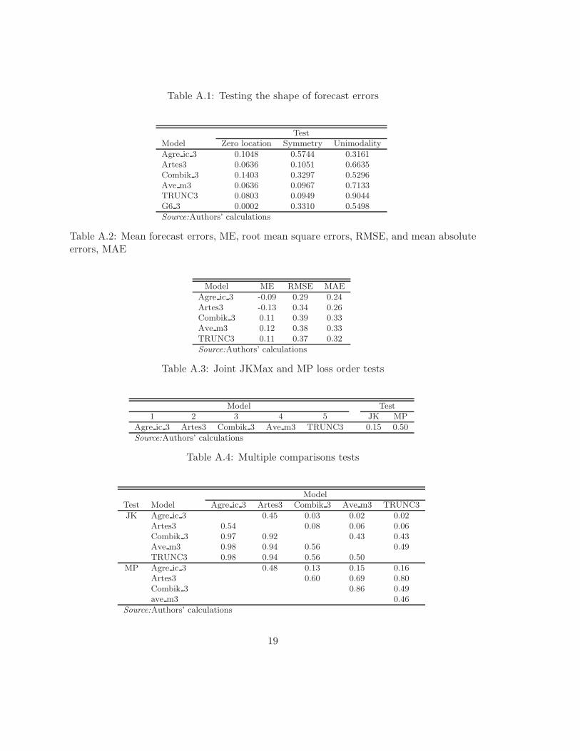
Table A.1: Testing the shape of forecast errors

TestModel Zero location Symmetry Unimodality

Agre ic 3 0.1048 0.5744 0.3161Artes3 0.0636 0.1051 0.6635Combik 3 0.1403 0.3297 0.5296Ave m3 0.0636 0.0967 0.7133TRUNC3 0.0803 0.0949 0.9044G6 3 0.0002 0.3310 0.5498

Source:Authors’ calculations

Table A.2: Mean forecast errors, ME, root mean square errors, RMSE, and mean absoluteerrors, MAE

Model ME RMSE MAE

Agre ic 3 -0.09 0.29 0.24Artes3 -0.13 0.34 0.26Combik 3 0.11 0.39 0.33Ave m3 0.12 0.38 0.33TRUNC3 0.11 0.37 0.32

Source:Authors’ calculations

Table A.3: Joint JKMax and MP loss order tests

Model Test1 2 3 4 5 JK MP

Agre ic 3 Artes3 Combik 3 Ave m3 TRUNC3 0.15 0.50

Source:Authors’ calculations

Table A.4: Multiple comparisons tests

ModelTest Model Agre ic 3 Artes3 Combik 3 Ave m3 TRUNC3

JK Agre ic 3 0.45 0.03 0.02 0.02Artes3 0.54 0.08 0.06 0.06Combik 3 0.97 0.92 0.43 0.43Ave m3 0.98 0.94 0.56 0.49TRUNC3 0.98 0.94 0.56 0.50

MP Agre ic 3 0.48 0.13 0.15 0.16Artes3 0.60 0.69 0.80Combik 3 0.86 0.49ave m3 0.46

Source:Authors’ calculations

19

Figure B.1: Power of JKMax and MP=GW for k = 2: ρ = 0 (left panel) and ρ = 0.25 (right panel)

0.0 0.2 0.4 0.6 0.8 1.0

0.1

0.2

0.3

0.4

0.5

0.6

n = 12

µ

k(µ)

JKmax

MP

0.0 0.2 0.4 0.6 0.8 1.0

0.1

0.2

0.3

0.4

n = 12

µ

k(µ)

JKmax

MP

0.0 0.2 0.4 0.6 0.8 1.0

0.2

0.4

0.6

0.8

1.0

n = 30

µ

k(µ)

JKmax

MP

0.0 0.2 0.4 0.6 0.8 1.0

0.2

0.4

0.6

0.8

n = 30

µ

k(µ)

JKmax

MP

0.0 0.2 0.4 0.6 0.8 1.0

0.2

0.4

0.6

0.8

1.0

n = 100

µ

k(µ)

JKmax

MP

0.0 0.2 0.4 0.6 0.8 1.0

0.2

0.4

0.6

0.8

1.0

n = 100

µk(µ

)

JKmax

MP

Source:Authors’ calculations

Figure B.2: Power of JKMax and MP for k = 3: ρ = 0 (left panel) and ρ = 0.25 (right panel)

0.0 0.2 0.4 0.6 0.8 1.0

0.2

0.4

0.6

0.8

1.0

n = 12

µ

k(µ)

JKmax

MP

0.0 0.2 0.4 0.6 0.8 1.0

0.2

0.4

0.6

0.8

n = 12

µ

k(µ)

JKmax

MP

0.0 0.2 0.4 0.6 0.8 1.0

0.2

0.4

0.6

0.8

1.0

n = 30

µ

k(µ)

JKmax

MP

0.0 0.2 0.4 0.6 0.8 1.0

0.2

0.4

0.6

0.8

1.0

n = 30

µ

k(µ)

JKmax

MP

0.0 0.2 0.4 0.6 0.8 1.0

0.2

0.4

0.6

0.8

1.0

n = 100

µ

k(µ)

JKmax

MP

0.0 0.2 0.4 0.6 0.8 1.0

0.2

0.4

0.6

0.8

1.0

n = 100

µ

k(µ)

JKmax

MP

Source:Authors’ calculations

20

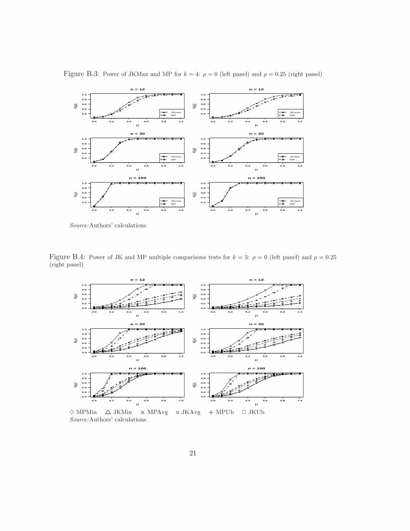
Figure B.3: Power of JKMax and MP for k = 4: ρ = 0 (left panel) and ρ = 0.25 (right panel)

0.0 0.2 0.4 0.6 0.8 1.0

0.2

0.4

0.6

0.8

1.0

n = 12

µ

k(µ)

JKmax

MP

0.0 0.2 0.4 0.6 0.8 1.0

0.2

0.4

0.6

0.8

1.0

n = 12

µ

k(µ)

JKmax

MP

0.0 0.2 0.4 0.6 0.8 1.0

0.2

0.4

0.6

0.8

1.0

n = 30

µ

k(µ)

JKmax

MP

0.0 0.2 0.4 0.6 0.8 1.0

0.2

0.4

0.6

0.8

1.0

n = 30

µ

k(µ)

JKmax

MP

0.0 0.2 0.4 0.6 0.8 1.0

0.2

0.4

0.6

0.8

1.0

n = 100

µ

k(µ)

JKmax

MP

0.0 0.2 0.4 0.6 0.8 1.0

0.2

0.4

0.6

0.8

1.0

n = 100

µ

k(µ)

JKmax

MP

Source:Authors’ calculations

Figure B.4: Power of JK and MP multiple comparisons tests for k = 3: ρ = 0 (left panel) and ρ = 0.25(right panel)

0.0 0.2 0.4 0.6 0.8 1.0

0.0

0.2

0.4

0.6

0.8

1.0

n = 12

µ

k(µ)

0.0 0.2 0.4 0.6 0.8 1.0

0.0

0.2

0.4

0.6

0.8

1.0

n = 12

µ

k(µ)

0.0 0.2 0.4 0.6 0.8 1.0

0.0

0.2

0.4

0.6

0.8

1.0

n = 30

µ

k(µ)

0.0 0.2 0.4 0.6 0.8 1.0

0.0

0.2

0.4

0.6

0.8

1.0

n = 30

µ

k(µ)

0.0 0.2 0.4 0.6 0.8 1.0

0.0

0.2

0.4

0.6

0.8

1.0

n = 100

µ

k(µ)

0.0 0.2 0.4 0.6 0.8 1.0

0.0

0.2

0.4

0.6

0.8

1.0

n = 100

µ

k(µ)

MPMin JKMin × MPAvg JKAvg + MPUb JKUbSource:Authors’ calculations

21

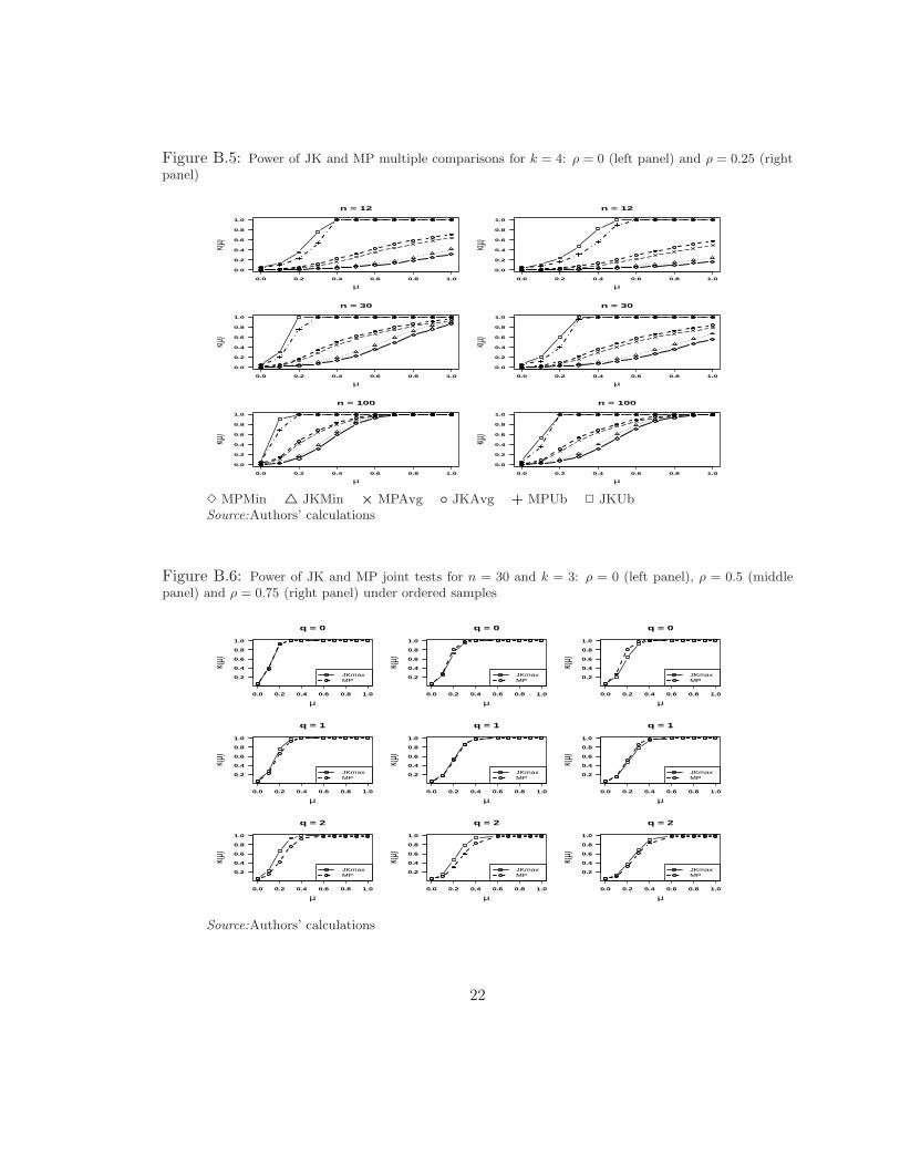
Figure B.5: Power of JK and MP multiple comparisons for k = 4: ρ = 0 (left panel) and ρ = 0.25 (rightpanel)

0.0 0.2 0.4 0.6 0.8 1.0

0.0

0.2

0.4

0.6

0.8

1.0

n = 12

µ

k(µ)

0.0 0.2 0.4 0.6 0.8 1.0

0.0

0.2

0.4

0.6

0.8

1.0

n = 12

µ

k(µ)

0.0 0.2 0.4 0.6 0.8 1.0

0.0

0.2

0.4

0.6

0.8

1.0

n = 30

µ

k(µ)

0.0 0.2 0.4 0.6 0.8 1.0

0.0

0.2

0.4

0.6

0.8

1.0

n = 30

µ

k(µ)

0.0 0.2 0.4 0.6 0.8 1.0

0.0

0.2

0.4

0.6

0.8

1.0

n = 100

µ

k(µ)

0.0 0.2 0.4 0.6 0.8 1.0

0.0

0.2

0.4

0.6

0.8

1.0

n = 100

µk(µ

)

MPMin JKMin × MPAvg JKAvg + MPUb JKUbSource:Authors’ calculations

Figure B.6: Power of JK and MP joint tests for n = 30 and k = 3: ρ = 0 (left panel), ρ = 0.5 (middlepanel) and ρ = 0.75 (right panel) under ordered samples

0.0 0.2 0.4 0.6 0.8 1.0

0.2

0.4

0.6

0.8

1.0

q = 0

µ

k(µ)

JKmaxMP

0.0 0.2 0.4 0.6 0.8 1.0

0.2

0.4

0.6

0.8

1.0

q = 0

µ

k(µ)

JKmaxMP

0.0 0.2 0.4 0.6 0.8 1.0

0.2

0.4

0.6

0.8

1.0

q = 0

µ

k(µ)

JKmaxMP

0.0 0.2 0.4 0.6 0.8 1.0

0.2

0.4

0.6

0.8

1.0

q = 1

µ

k(µ)

JKmaxMP

0.0 0.2 0.4 0.6 0.8 1.0

0.2

0.4

0.6

0.8

1.0

q = 1

µ

k(µ)

JKmaxMP

0.0 0.2 0.4 0.6 0.8 1.0

0.2

0.4

0.6

0.8

1.0

q = 1

µ

k(µ)

JKmaxMP

0.0 0.2 0.4 0.6 0.8 1.0

0.2

0.4

0.6

0.8

1.0

q = 2

µ

k(µ)

JKmaxMP

0.0 0.2 0.4 0.6 0.8 1.0

0.2

0.4

0.6

0.8

1.0

q = 2

µ

k(µ)

JKmaxMP

0.0 0.2 0.4 0.6 0.8 1.0

0.2

0.4

0.6

0.8

1.0

q = 2

µ

k(µ)

JKmaxMP

Source:Authors’ calculations

22

Figure B.7: Power of JK and MP joint tests for n = 30 and k = 4: ρ = 0 (left panel), ρ = 0.5 (middlepanel) and ρ = 0.75 (right panel) under ordered samples

0.0 0.2 0.4 0.6 0.8 1.0

0.2

0.4

0.6

0.8

1.0

q = 0

µ

k(µ)

JKmax

MP

0.0 0.2 0.4 0.6 0.8 1.0

0.2

0.4

0.6

0.8

1.0

q = 0

µ

k(µ)

JKmax

MP

0.0 0.2 0.4 0.6 0.8 1.0

0.2

0.4

0.6

0.8

1.0

q = 0

µ

k(µ)

JKmax

MP

0.0 0.2 0.4 0.6 0.8 1.0

0.2

0.4

0.6

0.8

1.0

q = 1

µ

k(µ)

JKmax

MP

0.0 0.2 0.4 0.6 0.8 1.0

0.2

0.4

0.6

0.8

1.0

q = 1

µ

k(µ)

JKmax

MP

0.0 0.2 0.4 0.6 0.8 1.0

0.2

0.4

0.6

0.8

1.0

q = 1

µ

k(µ)

JKmax

MP

0.0 0.2 0.4 0.6 0.8 1.0

0.2

0.4

0.6

0.8

1.0

q = 2

µ

k(µ)

JKmax

MP

0.0 0.2 0.4 0.6 0.8 1.0

0.2

0.4

0.6

0.8

1.0

q = 2

µ

k(µ)

JKmax

MP

0.0 0.2 0.4 0.6 0.8 1.0

0.2

0.4

0.6

0.8

1.0

q = 2

µ

k(µ)

JKmax

MP

Source:Authors’ calculations

Figure B.8: Power of JK and MP multiple comparisons tests for n = 30 and k = 3: ρ = 0 (left panel),ρ = 0.5 (middle panel) and ρ = 0.75 (right panel) under ordered samples

0.0 0.2 0.4 0.6 0.8 1.0

0.0

0.2

0.4

0.6

0.8

1.0

q = 0

µ

k(µ)

0.0 0.2 0.4 0.6 0.8 1.0

0.0

0.2

0.4

0.6

0.8

1.0

q = 0

µ

k(µ)

0.0 0.2 0.4 0.6 0.8 1.0

0.0

0.2

0.4

0.6

0.8

1.0

q = 0

µ

k(µ)

0.0 0.2 0.4 0.6 0.8 1.0

0.0

0.2

0.4

0.6

0.8

1.0

q = 1

µ

k(µ)

0.0 0.2 0.4 0.6 0.8 1.0

0.0

0.2

0.4

0.6

0.8

1.0

q = 1

µ

k(µ)

0.0 0.2 0.4 0.6 0.8 1.0

0.0

0.2

0.4

0.6

0.8

1.0

q = 1

µ

k(µ)

0.0 0.2 0.4 0.6 0.8 1.0

0.0

0.2

0.4

0.6

0.8

1.0

q = 2

µ

k(µ)

0.0 0.2 0.4 0.6 0.8 1.0

0.0

0.2

0.4

0.6

0.8

1.0

q = 2

µ

k(µ)

0.0 0.2 0.4 0.6 0.8 1.0

0.0

0.2

0.4

0.6

0.8

1.0

q = 2

µ

k(µ)

MPMin JKMin × MPAvg JKAvg + MPUb JKUbSource:Authors’ calculations

23

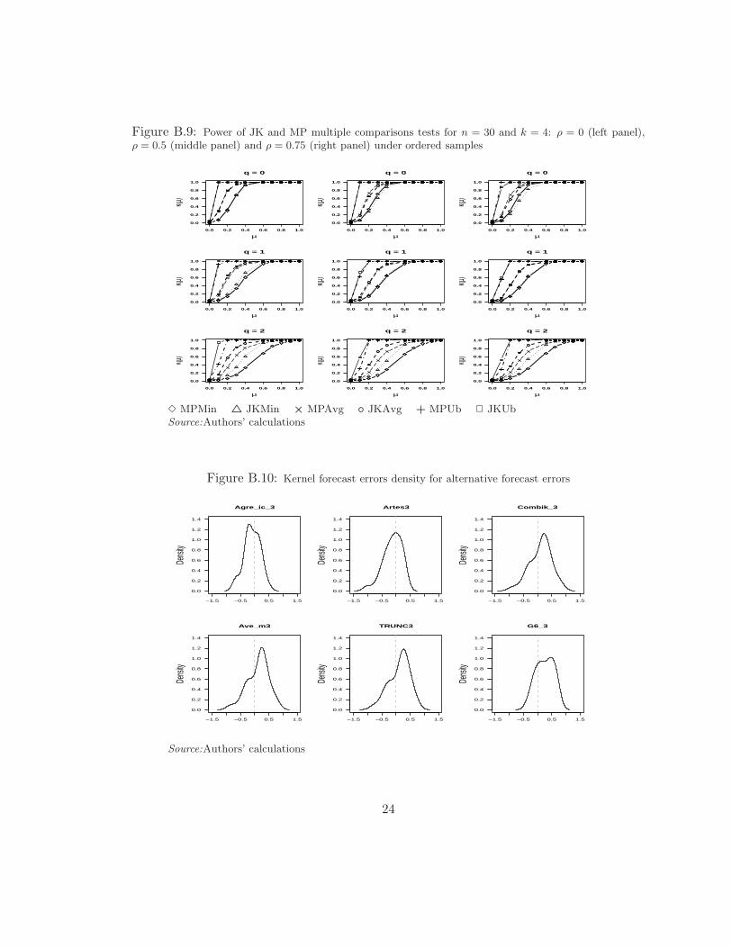
Figure B.9: Power of JK and MP multiple comparisons tests for n = 30 and k = 4: ρ = 0 (left panel),ρ = 0.5 (middle panel) and ρ = 0.75 (right panel) under ordered samples

0.0 0.2 0.4 0.6 0.8 1.0

0.0

0.2

0.4

0.6

0.8

1.0

q = 0

µ

k(µ)

0.0 0.2 0.4 0.6 0.8 1.0

0.0

0.2

0.4

0.6

0.8

1.0

q = 0

µ

k(µ)

0.0 0.2 0.4 0.6 0.8 1.0

0.0

0.2

0.4

0.6

0.8

1.0

q = 0

µ

k(µ)

0.0 0.2 0.4 0.6 0.8 1.0

0.0

0.2

0.4

0.6

0.8

1.0

q = 1

µ

k(µ)

0.0 0.2 0.4 0.6 0.8 1.0

0.0

0.2

0.4

0.6

0.8

1.0

q = 1

µk(µ

)0.0 0.2 0.4 0.6 0.8 1.0

0.0

0.2

0.4

0.6

0.8

1.0

q = 1

µ

k(µ)

0.0 0.2 0.4 0.6 0.8 1.0

0.0

0.2

0.4

0.6

0.8

1.0

q = 2

µ

k(µ)

0.0 0.2 0.4 0.6 0.8 1.0

0.0

0.2

0.4

0.6

0.8

1.0

q = 2

µ

k(µ)

0.0 0.2 0.4 0.6 0.8 1.0

0.0

0.2

0.4

0.6

0.8

1.0

q = 2

µ

k(µ)

MPMin JKMin × MPAvg JKAvg + MPUb JKUbSource:Authors’ calculations

Figure B.10: Kernel forecast errors density for alternative forecast errors

−1.5 −0.5 0.5 1.5

0.0

0.2

0.4

0.6

0.8

1.0

1.2

1.4

Agre_ic_3

Dens

ity

−1.5 −0.5 0.5 1.5

0.0

0.2

0.4

0.6

0.8

1.0

1.2

1.4

Artes3

Dens

ity

−1.5 −0.5 0.5 1.5

0.0

0.2

0.4

0.6

0.8

1.0

1.2

1.4

Combik_3

Dens

ity

−1.5 −0.5 0.5 1.5

0.0

0.2

0.4

0.6

0.8

1.0

1.2

1.4

Ave_m3

Dens

ity

−1.5 −0.5 0.5 1.5

0.0

0.2

0.4

0.6

0.8

1.0

1.2

1.4

TRUNC3

Dens

ity

−1.5 −0.5 0.5 1.5

0.0

0.2

0.4

0.6

0.8

1.0

1.2

1.4

G6_3

Dens

ity

Source:Authors’ calculations

24

Figure B.11: Kernel loss density estimate for alternative forecast procedures

0.0 0.2 0.4 0.6 0.8 1.0 1.2

0

2

4

6

8

loss

Dens

ity

Agre_ic_3Artes3

0.0 0.2 0.4 0.6 0.8 1.0 1.2

0

2

4

6

8

loss

Dens

ity

Agre_ic_3Combik_3

0.0 0.2 0.4 0.6 0.8 1.0 1.2

0

2

4

6

8

loss

Dens

ity

Agre_ic_3Ave_m3

0.0 0.2 0.4 0.6 0.8 1.0 1.2

0

2

4

6

8

loss

Dens

ity

Agre_ic_3TRUNC3

Source:Authors’ calculations

Figure B.12: Multiple comparison stochastic order results through JK pairwise tests

Source:Authors’ calculations

25

Figure B.13: Kernel distribution loss estimate for alternative forecast procedures

0.0 0.2 0.4 0.6 0.8 1.0 1.2

0.0

0.2

0.4

0.6

0.8

1.0

n=30, Bandwidth=0.046

kerne

l den

sity cu

mulat

ive

Agre_ic_3Artes3Combik_3TRUNC3

Source:Authors’ calculations

26