Search Frictions and the Labor Wedge

Andrea Pescatori and Murat Tasci

WP/11/117

© 2011 International Monetary Fund WP/11/117

IMF Working Paper

Research Department

Search Frictions and the Labor Wedge

Prepared by Andrea Pescatori and Murat Tasci1

Authorized for distribution by Abdul de Guia Abiad

May 2011

Abstract

This paper shows that labor market search frictions do not explain fluctuations in the labor wedge per se. However, the introduction of extensive and intensive margin clarifies that measuring the MRS in terms of total hours artificially introduces procyclicality in the MRS. When the MRS is correctly measured in terms of hours per worker, the labor wedge obtained is less variable than the one of the competitive model. Finally, we show that it is possible to measure a strongly procyclical labor wedge when the actual data generating process is a search model that allows for movements in both margins.

JEL Classification Numbers:E24; E32; J64

Keywords: Labor Market Search; Business Cycle Accounting; Labor Wedge

Author’s E-Mail Address: apescatori (at) imf.org; murat.tasci (at) clev.frb.org

This Working Paper should not be reported as representing the views of the IMF. The views expressed in this Working Paper are those of the author(s) and do not necessarily represent those of the IMF or IMF policy. Working Papers describe research in progress by the author(s) and are published to elicit comments and to further debate.

1 Murat Tasci is Research Economist at the Federal Reserve Bank of Cleveland; the views stated herein are those of the authors and are not necessarily those of the Federal Reserve Bank of Cleveland or of the Board of Governors of the Federal Reserve System. The authors would like to thank David Arseneau, Sanjay Chugh, Charles Carlstrom, Tim Fuerst, and seminar participants at the Federal Reserve Bank of Cleveland, the Federal Reserve Bank of Boston, and the Board of Governors of the Federal Reserve System.

- 2 -

Contents

I. Introduction . . . . . . . . . . . . . . . . . . . . . . . . . . . . . . . . . . . . . 3

II. Related Literature . . . . . . . . . . . . . . . . . . . . . . . . . . . . . . . . . 4

III. The prototype real business cycle model . . . . . . . . . . . . . . . . . . . . . . 5

IV. Introducing Search Frictions and Employment Fluctuations . . . . . . . . . . . 7A. Households . . . . . . . . . . . . . . . . . . . . . . . . . . . . . . . . . . . 8B. Firms . . . . . . . . . . . . . . . . . . . . . . . . . . . . . . . . . . . . . . 10C. Employment Contract and the Nash Bargaining . . . . . . . . . . . . . . 11D. Equilibrium . . . . . . . . . . . . . . . . . . . . . . . . . . . . . . . . . . 11E. The Wage Determination . . . . . . . . . . . . . . . . . . . . . . . . . . . 12F. The labor wedge . . . . . . . . . . . . . . . . . . . . . . . . . . . . . . . . 13

V. Results . . . . . . . . . . . . . . . . . . . . . . . . . . . . . . . . . . . . . . . . 16A. Mapping the Models to the U.S. data . . . . . . . . . . . . . . . . . . . . 16B. Mapping with the simulated data . . . . . . . . . . . . . . . . . . . . . . 22

VI. Conclusion . . . . . . . . . . . . . . . . . . . . . . . . . . . . . . . . . . . . . . 24

Appendices . . . . . . . . . . . . . . . . . . . . . . . . . . . . . . . . . . . . . . . . . 241. Appendix 1 . . . . . . . . . . . . . . . . . . . . . . . . . . . . . . . . . . . 25

1. Data . . . . . . . . . . . . . . . . . . . . . . . . . . . . . . . . . . . 252. Appendix 2 . . . . . . . . . . . . . . . . . . . . . . . . . . . . . . . . . . . 25

1. Households’Decision Problem . . . . . . . . . . . . . . . . . . . . . 252. Firms’Decision Problem . . . . . . . . . . . . . . . . . . . . . . . . 263. Details of Employment Contract . . . . . . . . . . . . . . . . . . . . 26

References . . . . . . . . . . . . . . . . . . . . . . . . . . . . . . . . . . . . . . . . . . 27

Tables

1. Moments and Correlations: High Frisch Elasticity . . . . . . . . . . . . . . . . 192. Moments and Correlations: Low Frisch Elasticity . . . . . . . . . . . . . . . . . 223. Simulation Exercise . . . . . . . . . . . . . . . . . . . . . . . . . . . . . . . . . 24

Figures

1. Labor Wedge in the RBC Model . . . . . . . . . . . . . . . . . . . . . . . . . . 72. Total Hours: Extensive vs. Intensive Margin . . . . . . . . . . . . . . . . . . . 153. The MRS and MPL in the Prototype Model . . . . . . . . . . . . . . . . . . . 174. Prototype vs. Search Model: Low Frequency . . . . . . . . . . . . . . . . . . . 185. Prototype vs. Search Model: Business Cycle Frequency . . . . . . . . . . . . . 206. Prototype vs. Search Model: Low Frequancy and low Frisch Elasticity . . . . 207. Prototype vs. Search Model: Business Cycle Frequency and Low Frisch Elasticity 218. Simulated Data: Labor Wedge and Output . . . . . . . . . . . . . . . . . . . . 23

- 3 -

I. Introduction

Real business cycle (RBC) models (i.e. Kydland and Prescott, 1982) impose a strongdiscipline on the choice of consumption and hours, both intertemporally andintratemporally. In these models, the optimal choice of hours is determined in equilibriumsuch that the marginal rate of substitution between consumption and leisure (mrs) isequal to the marginal productivity of labor (mpl). However, the data tell that there is asubstantial wedge between these two quantities that strongly co-varies with the economiccycle. In their seminal work, Chari Kehoe and McGrattan (2007) (henceforth CKM)conclude that, along with the effi ciency wedge, the labor wedge accounts for most of thefluctuations in output, putting it at the center of their business cycle accounting researchprogram.1

We interpret this finding as an indication of a significant misspecification of the prototypeRBC model as it relates to the labor market. Search and matching frictions (Mortensenand Pissarides 1994, Pissarides 2000) introduce a wedge between the wage and both thempl and the mrs, providing a natural framework to address misspecification related to thelabor market imperfections. It is indeed tempting to think that these type of frictions willinduce endogenous movements in the optimal choice of hours that could manifestthemselves as labor wedge. In this paper, we first present a model with labor marketfrictions– in the form of search and matching– that nests a prototype RBC model a laCKM; then, we ask whether the labor wedge, as usually measured, could be an artifact ofthese frictions and if so to what extent.

We find that a model with Nash bargaining between the firm and the marginal worker overhours and wage alter the firm’s perceived benefit of an additional hour at the intensivemargin (i.e. hours per employed worker), which is valued in terms of additional marginaloutput per worker. However, given that search frictions are internalized at the wagebargaining stage the equation that determines the labor wedge is not affected by searchfrictions directly or explicitly. Nevertheless, since fluctuations in total hours can now beattributed to both the intensive and extensive margin, the marginal rate of substitution,and thus the labor wedge, differ from the one implied by the prototype RBC model. Itturns out that the modification is in the right direction, that is the labor wedge we obtainis less variable and procyclical than the prototype labor wedge. This result is sensitive tothe exact parameterization of the labor supply elasticity. We find that, for instance, whenthe Frisch elasticity is relatively high, such as 2.8, as in most macro models, we can get upto 20 percent decline in the variability of the labor wedge– similarly, we find a reductionin the procyclicality. This result is even stronger, a 40 percent reduction, for Frischelasticities that are more consistent with the micro estimates.

We complement our results with a numerical exercise where we treat the search model asthe data generating process and describe the behavior of the labor wedge that aneconometrician would recover in doing business cycle accounting. We show that, even

1The business cycle accounting research program has the goal of identifying promising modeling avenuesfor dynamic general equilibrium models by measuring the "discrepancy" between the data and a prototypereal business cycle model. CKM identify four wedges: the effi ciency, labor, investment and governmentconsumption wedge. The labor and effi ciency wedge are considered the most important, suggesting thatmacro models that would like to explain real macro fluctuations should pay more attention to understandingwhat type of frictions could manifest themselves as these wedges.

- 4 -

though theoretically there is no labor wedge in the simulated data, one can falsely measurea significantly procyclical and variable labor wedge if the underlying search frictions andthe explicit distinction between the intensive and the extensive margin is ignored in themeasurement. About 15 percent of the relative variation in the labor wedge and all itscomovement with output and total hours could be explained by this misspecification.

The next section discusses the related literature, especially that on the business cycleaccounting and the labor wedge. Section 3 presents the idea behind the business cycleaccounting exercise in CKM using US data, and puts our following exercise in a context.Section 4 presents an extension of the prototype RBC model with search frictions anddiscusses how search frictions imply a different labor wedge. Section 5 shows,quantitatively, how search frictions alter the measured wedge, first by using the US dataand focusing on only one equilibrium condition, then by using the model generated dataand analyzing the behavior of labor wedge in these simulations. Section 6 concludes.

II. Related Literature

This paper is part of the vast literature that studies labor market imperfections inconnection with the business cycle, such as in Mortensen and Pissarides (1994), Cole andRogerson (1999), and Shimer (2005), among others. However, the extension of thestandard growth model we use is most closely related to Andolfatto (1996) and Merz(1995, 1999), which embed search frictions into an otherwise standard RBC model.

The focus on the labor wedge makes the paper naturally related to the recent literature onbusiness cycle accounting, which, in different forms, dates back before CKM.2 Forexample, Hall (1997) identifies variations in the marginal rate of substitution as animportant element to explain aggregate fluctuations. Several other studies in theliterature focused on the same equilibrium condition in the labor market and provideddifferent interpretations of it, ranging from changes in labor market institutions,competitive structure of the economy, price-wage markup, changes in regulation, and taxpolicy (see in particular, Cole and Ohanian 2002, Gali, Gertler and Lopez-Salido 2007,Mulligan 2002, Rotemberg and Woodford 1991 and 1999). Chang and Kim (2007), on theother hand, argues that the apparent distortion in the labor market clearing condition asmeasured in the aggregate data might be partly due to aggregation bias. They show thata heterogenous-agent economy with incomplete capital markets and indivisible labor cangenerate this observed wedge. Arseneau and Chugh (2010) also anlayze a generalequilibrium matching model with distortions that map into a measured labor wedge. Eventhough the focus is on optimal tax policy, they show that, as in our paper, labor wedgetakes two different forms with matching frictions, one intratemporal and oneintertemporal.

More recently, Blanchard and Gali (2010), Cheremukhin and Restrepo-Echavarria (2010)and Shimer (2009, 2010) focus on the variation in the labor wedge. Shimer (2009) reviewsthe literature and makes a case for focusing the attention on the labor wedge, as it isrelatively immune to how the model environment is specified and the expectations are

2One can trace the basic idea behind this exercise to early work in the RBC literature as in Prescott(1986) or Ingram, Kocherlakota and Savin (1994).

- 5 -

formed. Cheremukhin and Restrepo-Echavarria (2010) lays out an RBC model withsearch frictions and argues that most of the variation in the labor wedge is attributable tothe residual shock to matching effi ciency, rather than variations in job destruction orimpediments to the bargaining process. Both Blanchard and Gali (2010) and Shimer(2010), differ in their formulation of the search frictions from us, and derive a neutralityresult. This result basically implies that fluctuations in the unemployment rate areindependent of the aggregate productivity. In Blanchard and Gali (2010), this is due tofact that recruitment of firms is not affected by aggregate productivity. As Shimer (2010)argues, this follows when one assumes that recruitment is only labor-intensive, not goodintensive. We favor a more traditional approach, as in Andolfatto (1996) and Merz (1995)and model recruitment as a good-intensive technology and hence firms respond toproductivity shocks by increasing recruitment during booms. We find it reasonable toassume that, at least partially, firms cannot just bear the cost of recruitment by costlesslyswitching workers from production to recruitment in response to productivity shocks.

III. The prototype real business cycle model

In this section we present a prototype business cycle model with perfectly competitivefactor markets. As we will see, when the model is taken to the data, the theoreticalprediction that the marginal rate of substitution between consumption and leisure has tobe equal to the marginal productivity of labor does not hold; following the literature, wename this discrepancy labor wedge.

The economy is populated by a continuum of mass 1 of identical households solving adynamic optimization problem over the choices of consumption (ct), savings (xt) andhours worked (ht). Markets are complete and household utility function is separable inconsumption and leisure. Households maximize their expected utility3

E0∞∑t=0

βt[U (ct) + ψG(ht)], 0 < β < 1, (1)

where β is the subjective discount factor, ct is consumption and ht is per capita hoursworked in period t. Households earn wages wt and receive rental income, rt, from capitalthat they rent out to firms. They can invest xt units each period which adds to newcapital next period, kt+1, net of depreciation, δ. Wedges operate as a tax, following CKMwe introduce a tax on investment and labor earnings, [1 + εx,t] and [1− εl,t], respectively.Finally, in each period, households also receive a lump sum transfer, Tt, from government.Let W h(·) and W f (·) denote the value functions for households and firms respectively.Then, we can summarize the household optimization problem as follows

W h(ωt) = maxct,kt+1,xt,lt

U (ct) + ψG(ht) + βEtW h(ωt+1|ωt) (2)

s.t. ct + xt [1 + εx,t] = wt [1− εl,t]ht + rtkt + Tt (3)

kt+1 = (1− δ)kt + xt (4)

3Usual restricions on the functional form apply, that is Uc (c) > 0 , Ucc (c) ≤ 0 , Gh(h) < 0, and Ghh(h) ≤0 as well as usual Inada conditions. In addition, we normalize G(0) = 0 and impose G(h) < 0, ∀h > 0.

- 6 -

where ωt = kt,Ωt is the set of individual and aggregate state variables, respectively.Optimality requires the net wage to be equal to the marginal rate of substitution betweenconsumption and leisure, mrs; given that all households are identical, this conditionbecomes the relevant labor supply schedule

[1− εl,t]wt = −ψGh(ht)/Uc (ct) ≡ mrst.

Firms hire workers and capital to produce according to a neoclassical production functionεz,tf(kt, lt), where εz,t is the exogenous productivity shock (or effi ciency wedge) and lrepresents total hours demanded by the firm, the product of hours per worker h andemployment n. For future comparison we also write down the static firm optimization in aconsistent way.

W f (ωt) = maxkt,ht,nt

εz,tf(kt, htnt)− wthtnt − rkt (5)

Optimality requires the wage to be equal to the marginal productivity of labor,given thatall firms are identical this condition becomes the relevant labor demand schedule4

wt = εz,tfl(kt, lt) ≡ mplt.

Finally, we assume that the government runs a balanced budget in each period such thattax revenues are equal to government spending Tt + xtεx,t + wtltεl,t = εg,t.

In equilibrium we assume that the labor market is always at full employment, nt = 1;hence, we can replace hours per worker with total hours ht = lt.5 The followingconditions describe the competitive equilibrium

Uc(ct) [1 + εx,t] = βEt[Uc(ct+1)[εz,t+1fk(kt+1, lt+1) + (1− δ) (1 + εx,t+1)]|ωt] (6)

mrst(lt) = −ψGh(lt)/Uc (ct) = mplt [1− εl,t] (7)

εz,tf(kt, lt) = ct + kt+1 − (1− δ)kt + εg,t (8)

along with a set of unique realizations for the vector of exogenous process εt =[εx,t, εl,t, εz,t, εg,t]. Notice that the equation that describes the labor market equilibrium isstatic and is the only one where εl,t appears. Under various functional forms– and once aparametrization is chosen– using data on output (yt), total hours (lt), and consumption(ct) is enough to pin down a unique value for the labor tax rate εl,t. If the actual labor taxrate does not vary substantially at business cycle frequency, [1− εl,t] can be interpreted asa discrepancy between the model and the data: a labor wedge (Shimer 2009). While wedo not attempt to draw causal implication as in CKM, we analyze the statisticalproperties of the labor wedge in relation to business cycles. Figure (1) plots [1− εl,t] overthe period 1959:I to 20010:III (in the figure, the historical realizations of [1− εlt] areaccording to the measurement equation (7) and data on yt, ct, and lt are over the period

4Notice that once the marginal productivity of labor is equal to the wage the firm is also indifferentbetween the extensive and intensive margin.

5 It is worth noting that the household problem could be recast in terms of a big family that equalizesconsumption across its members and maximizes the momentary utility function U (ct) + ψntG(ht). In thebudget constraint labor income would be (1 − εt)wtnth with the additional constraint nt ≤ 1. In general,the full emplyment constraint would be binding and, thus, we would have the same equilibrium conditionsshown in the text. In the next section we will make explicit use of this setting.

- 7 -

Figure 1. Labor Wedge in the RBC Model

1959:1 to 2010:III. Shaded areas indicate NBER recession dates). The labor wedge seemsto have a low frequency movement, which might be explained by changes in the taxes (seefor instance, Ohanian, Rogerson and Raffo, 2008) or changes in the composition of theworkforce and the resulting imperfect household aggregation over-time (Cociuba andUeberfeldt, 2010). However, at the business cycle frequency, there is a lot of variation inthe measured labor wedge that is highly unlikely to be explained by high-frequencychanges in labor tax. Moreover, the figure confirms the well known result that the laborwedge, [1− εl,t], is pro-cyclical (falling during recessions) and is positively correlated withper capita hours worked.

In the next section we explore how a model with frictions in the labor market and with anextensive and intensive labor margin can help explain the observed discrepancy betweenthe marginal rate of substitution and the marginal productivity of labor.

IV. Introducing Search Frictions and EmploymentFluctuations

The model economy is almost identical to the one presented in the preceding sectionexcept for the presence of search and matching frictions in the labor market andmovements in both the intensive and the extensive margin for labor. In other words, eventhough goods and capital are exchanged in perfectly competitive markets, labor marketimperfections allow for unemployment. The model is a decentralized version of Andolfatto(1996) and Merz (1995) and is laid out such that it looks similar to the prototype realbusiness cycle (RBC) model previously described. Search frictions in the model aresummarized at an aggregate level by an aggregate matching function and requirehouseholds and firms to determine employment contracts through Nash bargaining. Wefirst provide the details of the problem for households and firms and then discuss the Nash

- 8 -

bargaining outcome.

A. Households

The economy is populated by a continuum of infinitely-lived worker-householdsdistributed uniformly along the unit interval implying a constant labor force normalized toone. At any point in time, only a mass nt ≤ 1 of households is employed while theremaining 1− nt households are unemployed and searching for a job. Each household hasthe same utility function as in the previous section. Markets are complete providingperfect insurance against unemployment risk, hence, consumption is equalized acrosshouseholds (Andolfatto 1996 and Merz 1995). It is easy to prove that we can recast theproblem in terms of a representative household that maximizes the sum of each individualhousehold expected utility

E0∞∑t=0

βt[U (ct) + ψntG(ht)], 0 < β < 1. (9)

The objective function of the representative household differs from the one of theprototype model because it explicitly takes into account the possibility that employmentmay vary over time– when nt ≡ 1 we are back to the perfectly competitive model.6 Eachunemployed worker exerts some effort, et, to find a job, which costs c(et) units ofresources.7 As a result, the budget constraint of the representative households can bewritten as

ct + xt [1 + τx,t] + c(et)(1− nt) = wt [1− τ l,t]ntht + rtkt + Tt (10)

Note that τ l is the analog of εl in the prototype model, i.e. the fraction of labor earningsnet of taxes.

Given the complete markets assumption it is easy to write the law of motion for aggregatecapital

Kt+1 = (1− δ)Kt +Xt 0 ≤ δ ≤ 1. (11)

When households solve their problems, they are going to take wage, wt, and hours workedht as given, as they will be determined through Nash Bargaining (see next section). Weassume that trade in the labor market is mediated by an aggregate matching function thatdetermines the number of jobs formed in each period as a function of the number of jobvacancies, Vt, and the aggregate search effort of the household/workers, (1−Nt)Et

Mt = τχ,tVγt [(1−Nt)Et]

1−γ (12)

where 0 < γ < 1, τχ,t is the period-t realization of a process that governs the effi ciency ofmatching, and the following intuitive restriction applies Mt ≤ min Vt, 1−Nt. Using thedefinition of the matching function, we can write the probability of finding a job for anunemployed worker as pt = Mt

(1−Nt)Et , which is taken as given at household level.

6Notice that we have made use of the normalization G(0) = 0. Hence the term (1 − nt)ψG(0) does notexplicitely appear in the objective function.

7Cost of search function, c(e), is assumed to be strictly convex and increasing in e.

- 9 -

Job matches that are formed in a period are assumed to become productive in thefollowing period. That is, they only increase employment with a one-period lag. As jobsare created, they are also being destroyed. Letting σ denote the period-t fraction ofexisting jobs destroyed, the law of motion for employment is given by the expression

Nt+1 = (1− σ)Nt +Mt, (13)

where σ ∈ [0, 1]. At the household level, employment nt evolves endogenously according tothe following, slightly modified equation of motion

nt+1 = (1− σ)nt + pt(1− nt)et. (14)

Let’s define the aggregate productivity shock, τ z,t as the analog of εz,t. We can finallywrite down the representative household problem recursively

W h(ωht ) = maxxt,etU (ct) + ψntG(ht) + βEtW h(ωht+1|ωht ) (15)

s.t. ct + xt [1 + τx,t] + c(et)(1− nt) = wt [1− τ l,t]ntht + rtkt + Tt (16)

nt+1 = (1− σ)nt + pt(1− nt)etkt+1 = (1− δ)kt + xt

taking wt = w(Ωt), rt = r(Ωt), pt = p(Ωt), and equations of motion for aggregate statevariables, Kt and Nt as given. For notational simplicity, let ωht = kt, nt,Ωt andΩt = τ t,Kt,Nt denote individual and aggregate state variables for the householdrespectively, with τ t = [τ l,t, τx,t, τ z,t, τ g,t, τκ,t] being the vector of exogenous processesanalogous to εt. This optimization problem leads to two conditions that determine theoptimal savings and search effort recursively for the large household (details are in theappendix):

Uc(ct) [1 + τx,t] = βEt[Uc(ct+1)(rt+1 + (1− δ) [1 + τx,t+1])|ωht

]. (17)

Uc(ct)ce(et)/pt = βEt

[Uc(ct+1)[wt+1 [1− τ l,t+1]ht+1 + c(et+1)]+

ψG(ht+1) + Uc(ct+1)ce(et+1)pt+1

(1− σ − pt+1et+1) |ωht

](18)

The first Euler equation is the standard consumption Euler equation. The second Eulerequation determines the households’optimal search behavior. The left hand side in (18) isthe expected marginal cost of search for the households in current consumption units,which should be equal to the expected marginal gains from search on the right hand side.If search is successful, the household expects to get utility from the net wage payments,wt+1 [1− τ l,t+1]ht+1, and from economizing on future search costs, c(et+1), and to getdisutility from working G(ht+1). The final term in brackets represents the net futurebenefit arising from the expected persistence of a job match.8 Note that, the household

8Given that any single current-period match survives with probability 1−σ, households’expected utilitywill increase simply by reducing expected future recruiting costs by the quantity Uc(ct+1)ce(et+1)

pt+1(1− σ).

The second term in this sum, −pt+1et+1 Uc(ct+1)ce(et+1)pt+1, represents the reduction in the future job-finding

rate, due to the current depletion of the unemployment stock.

- 10 -

decision for optimal saving is exactly identical to the one in the competitive model(equation 6). Hence, all things equal, labor market frictions do not affect the wedgebetween marginal utility of consumption and the expected real rate of return on capital inthe model. Instead, labor market frictions affect the search behavior, hence the laborsupply decision. Next we turn to the demand side and describe firms’problem.

B. Firms

As in the previous section firms operate a constant returns to scale production function,τ z,tf(kt, ntht) However, while capital is rented in a perfectly competitive market, firmsmust undergo a costly search process before jobs are created and output is produced. Foreach job vacancy created in period-t, firms pay κ units of output resulting in period-t“vacancy-posting”costs of κvt. Jobs must be posted as vacancies before they can be filled.We assume that vacancies adjust in equilibrium such that the value of an additionalvacancy is driven to zero. We are going to approach the firms’problem in two steps. Inthe first step, firms decide how much capital to rent and how many jobs to create takingthe rental rate rt, aggregate state variables, the labor contract wt, ht, and theprobability of filling a vacancy, qt, as given9

W f (ωft ) = maxkt,vt,nt+1

τ z,tf(kt, ntht)− wtntht − rtkt − κvt + βtEtWf (ωft+1|ω

ft ) (19)

such that f(kt, ntht) = kαt (ntht)(1−α) (20)

nt+1 = (1− σ)nt + qtvt

where ωft = kt, nt,Ωt, rt = r(Ωt), wt = w(Ωt) with Ωt = τ t,Kt,Nt andβt = βEt

[Uc(ct+1)Uc(ct)

]. Firms’problem in (19) impliesa set of first order conditions that

determine the optimal level of capital stock rented and the number of vacancies posted byfirms.

τ z,tfkt(kt, ntht)− rt = 0 (21)

κ

qt= βtEt

[τ z,t+1flt+1(kt+1, nt+1ht+1)ht+1 − wt+1ht+1 + (1− σ)

κ

qt+1|ωft]

(22)

The first condition is the familiar relation between the rental rate and the marginalproduct of capital. The second condition determines the optimal number of vacanciesposted by firms. It implies that the marginal cost of filling a vacancy should be equal tothe marginal benefit, in expectation. Since each vacancy costs κ and the duration of avacancy is expected to be 1/qt, κ

qtgives the expected marginal cost of filling one vacancy.

On the right hand side, we see how each additional filled job produces its marginalproduct next period net of wage payments, while the third term represents the expectedsaving in terms of future recruitment costs.

9From the aggregate matching function in (12), we know that the probability of filling a vacancy mustbe qt = Mt/Vt.

- 11 -

C. Employment Contract and the Nash Bargaining

Since negotiating a wage has an implicit opportunity cost due to search frictions, we needa mechanism to determine the surplus for each contracting party. It is standard in thesearch literature to use generalized Nash bargaining for this purpose (see for instance,Pissarides 2000). We follow the same approach and assume that each worker’semployment contract, wt, ht, is determined through Nash bargaining between the firmand the household. In a setting like this, where there are multiple workers within a firm,it is not entirely clear how to formulate the bargaining problem. Fortunately, Stole andZwiebel (1996) show that bargaining should happen over the marginal surplus for bothparties.10 11 Assuming that households (firms) have a bargaining power of 1− λ (λ) thegeneralized Nash bargaining problem takes the following form12

maxwt,ht

W hnt(ωt)

1−λW fnt(ωt)

λ (23)

where W hnt(ωt) is the household’s net marginal surplus from having one more worker

employed given household’s optimal behavior, and W fnt(ωt) is the firm’s net marginal

surplus from having one more employee given firm’s optimal behavior. As long as eachparty can extract some surplus, i.e. W h

nt(ωt) > 0 and W fnt(ωt) > 0, this Nash bargaining

problem yields two conditions that determine equilibrium level of hours, ht, and wage perhour, wt (details of the solution are presented in the Appendix)

λW hn (ωt)− (1− λ)(1− τ l,t)Uc(ct)W f

n (ωt) = 0 (24)

Uc(ct) [1− τ l,t] [τ z,tfl(kt, ntht) + τ z,tfll(kt, ntht)ntht] + ψGh(ht) = 0 (25)

Equation (24) is the starting point to determine the hourly wage and basically divides thetotal surplus of the marginal match among the household and the firm. Notice that τ l,texogenously reduces the household’s share of surplus and, at the limit τ l,t = 1, thehousehold’s surplus is zero W h

nt = 0. Household risk aversion adds a time-varyingdimension to the sharing rule: in times of high marginal utility households claim arelatively higher surplus. Equation (25) is the first order condition with respect to hours,as we will see this equation will play a crucial role in the analysis of the labor wedge.Those last two conditions complete the necessary set of equations that fully characterizethe equilibrium. Next, we combine these set of conditions to describe the recursivecompetitive equilibrium.

D. Equilibrium

Since all households and firms are identical, in equilibrium, individually effi cientallocations coincide with the aggregate, i.e. kt = Kt, ct = Ct, lt = Lt, nt = Nt, thereforethe relevant state is Ωt. Then the competitive equilibrium of this economy is

10For examples see Merz (1995), Beauchemin and Tasci (2008), Fujita and Nakajima (2009), and Elsbyand Micheals (2010), among others.11 Implicitly, we assume that the contracted hours apply to every worker. However, given that G(·) is

convex, it is easy to prove that homogenous hours minimize the overall worker disutility.12We drop the distinction between the state variables for the households and the firms, since in equilibrium,

ωht = ωft = ωt.

- 12 -

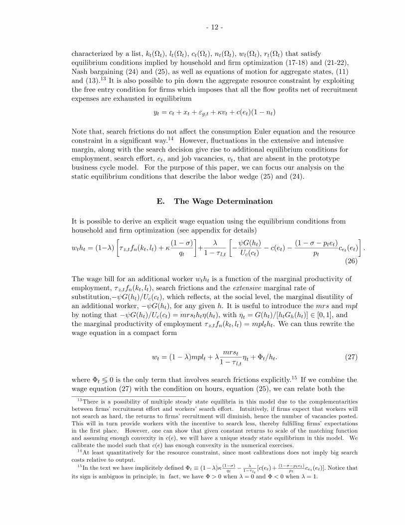
characterized by a list, kt(Ωt), lt(Ωt), ct(Ωt), nt(Ωt), wt(Ωt), rt(Ωt) that satisfyequilibrium conditions implied by household and firm optimization (17-18) and (21-22),Nash bargaining (24) and (25), as well as equations of motion for aggregate states, (11)and (13).13 It is also possible to pin down the aggregate resource constraint by exploitingthe free entry condition for firms which imposes that all the flow profits net of recruitmentexpenses are exhausted in equilibrium

yt = ct + xt + εg,t + κvt + c(et)(1− nt)

Note that, search frictions do not affect the consumption Euler equation and the resourceconstraint in a significant way.14 However, fluctuations in the extensive and intensivemargin, along with the search decision give rise to additional equilibrium conditions foremployment, search effort, et, and job vacancies, vt, that are absent in the prototypebusiness cycle model. For the purpose of this paper, we can focus our analysis on thestatic equilibrium conditions that describe the labor wedge (25) and (24).

E. The Wage Determination

It is possible to derive an explicit wage equation using the equilibrium conditions fromhousehold and firm optimization (see appendix for details)

wtht = (1−λ)

[τ z,tfn(kt, lt) + κ

(1− σ)

qt

]+

λ

1− τ l,t

[−ψG(ht)

Uc(ct)− c(et)−

(1− σ − ptet)pt

cet(et)

].

(26)

The wage bill for an additional worker wtht is a function of the marginal productivity ofemployment, τ z,tfn(kt, lt), search frictions and the extensive marginal rate ofsubstitution,−ψG(ht)/Uc(ct), which reflects, at the social level, the marginal disutility ofan additional worker, −ψG(ht), for any given h. It is useful to introduce the mrs and mplby noting that −ψG(ht)/Uc(ct) = mrsthtη(ht), with ηt = G(ht)/[htGh(ht)] ∈ [0, 1], andthe marginal productivity of employment τ z,tfn(kt, lt) = mpltht. We can thus rewrite thewage equation in a compact form

wt = (1− λ)mplt + λmrst

1− τ l,tηt + Φt/ht. (27)

where Φt ≶ 0 is the only term that involves search frictions explicitly.15 If we combine thewage equation (27) with the condition on hours, equation (25), we can relate both the13There is a possibility of multiple steady state equilibria in this model due to the complementarities

between firms’recruitment effort and workers’search effort. Intuitively, if firms expect that workers willnot search as hard, the returns to firms’recruitment will diminish, hence the number of vacancies posted.This will in turn provide workers with the incentive to search less, thereby fulfilling firms’ expectationsin the first place. However, one can show that given constant returns to scale of the matching functionand assuming enough convexity in c(e), we will have a unique steady state equilibrium in this model. Wecalibrate the model such that c(e) has enough convexity in the numerical exercises.14At least quantitatively for the resource constraint, since most calibrations does not imply big search

costs relative to output.15 In the text we have implicitely defined Φt ≡ (1−λ)κ (1−σ)

qt− λ

1−τlt[c(et)+ (1−σ−ptet)

ptcet(et)]. Notice that

its sign is ambiguos in principle, in fact, we have Φ > 0 when λ = 0 and Φ < 0 when λ = 1.

- 13 -

mrst and the mplt to the wage

wt = mplt[1− λ(1− ηtsLt )] + Φt/ht (28)

wt =mrst

1− τ l,t[1− λ(1− ηtsLt )]

sLt+ Φt/ht (29)

where we have introduced the output elasticity to total hours sLt = 1 + fll(kt,lt)ltfl(kt,lt)

∈ [0, 1],

which is approximately the labor share.16 Those two equations are very instructive andresemble the labor supply and labor demand equations of the perfectly competitive model.However, search frictions coupled with Nash bargaining introduce two time varying wedgesbetween the wage and both the marginal productivity of labor and the marginal rate ofsubstitution. In fact, even if τ l,t were constant, the wage would not perfectly co-vary withthe mpl and the mrs over the cycle, being affected by movements in the search frictionsΦt and in the way the match surplus is split. In general, the wage will be between the mrsand the mpl, however, when λ is small, it might be possible to observe wt > mplt. In partthis is due to the presence of sLt which reduces the firm’s perceived benefit of labor. Infact, firms value the benefit of increasing hours worked h across workers in terms of itseffect on the marginal productivity of an extra worker (not in terms of the average workerproductivity). However, while the cost is still linear in h, the marginal productivity ofemployment is not: as long as there is curvature in the production function, i.e., sL < 1,the marginal productivity of employment increases with h less than one-to-one.

Finally, it is also interesting to note that the firm bargaining power parameter, λ, isinversely related to the wage and enters symmetrically in both equations (28) and (29). Aswe will see, this implies that the bargaining power per se does not affect the labor wedge,as long as there is an interior solution of the Nash Bargaining problem, i.e., λ ∈ (0, 1).

In the following section we describe in more detail our labor wedge and compare it withthe one of the competitive model.

F. The labor wedge

Eliminating the wage from (28) and (29) we have an expression that is analogous to theone of the perfectly competitive model (equation 7).

mrst = mplt [1− τ l,t] sLt (30)

It is striking that while the bargaining process has created a wedge between mrs and mpl,search frictions per se do not appear directly in this equation. Mechanically, this is simplybecause they enter symmetrically and additively in the labor demand and supplyequations, hence, when those are equated search frictions perfectly offset and cancel out.The same is true also for λ and η which affect mrs and mpl exactly in the sameproportion. Intuitively, one reason for this result is that the bargaining processinternalizes search frictions through the wage rather than hours. In part this may be due

16 In the search model, due to the search frictions sL is not exactly the labor share– while it is in theperfectly competitive model.

- 14 -

to the fact that search frictions are inherently intertemporal– i.e. it takes time andresources to match unemployed workers with vacant positions– while the labor wedge isinherently intratemporal. The effects of intertemporal frictions are absorbed bymovements in the wage and the extensive margin, and not in the labor wedge.

In order to understand the effects of search frictions on the extensive margin, it is crucialto observe that the variation in this margin is governed by mainly two decisions; workers’search effort and firms’vacancy posting decision. Optimality conditions for search effortand vacancies (see equations 18 and 22) along with the law of motion for employment willgovern the movements at the extensive margin. Using equations (18) and (22), noting thatthe terms in expectations are each party’s marginal surplus from a match, one can writedown a simple equation that relates market tightness and search effort to movements inthe value of expected surpluses:

κθtetce(et)

=Et[Uc(ct+1)W

fnt+1

]Et[W hnt+1

] . (31)

Variations in the relative values of expected surpluses will determine fluctuations inmarket tightness, θt, and et, implying fluctuations in employment. Note also that theNash bargaining outcome requires a specific sharing rule determining the relation betweenW fnt and W

hnt for all t (see equation 24). Once this is taken into account, it is easy to see

how fundamental parameters related to search frictions explicitly affect the movements inthe extensive margin through search effort and market tightness. Up to a covariance termequation (31) can be written as17

κθtetce(et)

' λ

1− λEt1

1− τ l,t+1(32)

Equation (32) shows, how the labor wedge (that will be pinned down by equation 34below) affects the cost of searching and, thus, employment fluctuations. In turn, since theemployment law of motion has to hold, movements in the labor wedge will probablyinduce fluctuations in the matching function process, τχ, interpretable as the extensivelabor wedge. We leave the study of the extensie wedge to future work and focus on thestatic labor wedge instead.

Going back to the static condition (30), one can see that the only distortion present,summarized by sLt , is induced by the bargaining problem. However, once we assume thatthe production function takes a Cobb-Douglas form, such that fll(k, l)l = −αfl(k, l), themarginal productivity of workers change one-to-one with h, we have that sLt = 1− α.Hence, the wedge introduced by sLt is irrelevant at business cycle frequency. The constant(1− α) acts like a tax on employment, which, in this context, is observationally equivalentto a labor income tax; in the baseline calibration α takes a value of about 0.35 reducingsubstantially the steady state value required for τ l.18

17This is similar to the ‘intertemporal labor wedge’derived by Arseneau and Chugh (2010).18While a different functional form for the production function would imply a time-varying sL, we do not

believe that this will much help in explaining the cyclical properties of the labor wedge.

- 15 -

We can finally compare the two fundamental equations that are used to back out the laborwedge from the data in the competitive and non-competitive labor market model

[1− εl,t] =mrst(lt)

mplt= − ψ

mpltUc(ct)Gh(ntht) (33)

[1− τ l,t] =mrst(ht)

mplt

1

1− α = − ψ

mpltUc(ct)

Gh(ht)

1− α (34)

The major difference between the prototype labor wedge [1− εl,t] and ours is that, in theperfectly competitive RBC model the lack of distinction between the extensive andintensive margin has induced the use of total hours worked in the evaluation of the mrsinstead of hours per worker. Intuitively, the presence of nt in the prototype labor wedgeequation may introduce a strongly procyclical element– given that Gh > 0. Employmentis instead not present in the second equation when we back out our discrepancy, [1− τ l,t].Since movements in both margins are not equally significant in deriving the business cyclefrequency fluctuations in total hours, this distinction about the intensive-extensive marginis clearly important. Figure (2) shows the decomposition of total hours into itscomponents (plots for only employment and hours are generated keeping the respectivemargin moving where the other margin is assumed to be fixed at the historical average.Shaded areas indicate NBER recession dates). Total hours in the U.S. is clearlyprocyclical. When total hours is assumed to follow a path where one of the margins isfixed at its historical average and the other margin is assumed to follow the actual path inthe data, one recognizes the well-known fact that most of the fluctuations in total hourscomes from the extensive margin, not the intensive margin (Shimer 2009). This stylizedfact is particularly relevant when interpreting the results of our exercise.

Figure 2. Total Hours: Extensive vs. Intensive Margin

To see why this might affect the measured labor wedge, consider a simple constant Frischelasticity utility function of the form G(x) = −x(1+φ)/(1 + φ). Then we can write a simplerelation describing the mapping between [1− εl,t] and [1− τ l,t]

[1− εl,t] = (1− τ l,t)(1− α)nφt (35)

- 16 -

This shows how some of the observed procyclicality of [1− εl,t] induced by employmentdoes not have to be present in our labor wedge. In other words, even if we could interpretall the movements in τ l as due to actual changes in labor tax, equation (35) suggests thatwe would still find a strongly procyclical labor wedge [1− εl,t] in the prototype modelmerely because of procycilcal employment fluctuations in the data– the higher φ thestronger the procyclicality.

V. Results

In this section we present the results of our quantitative experiments. The labor wedge isa reduced form expression of a model’s inability to explain the data. Ideally, we wouldlike to have a truly exogenous and small wedge, that, excluding tax movements, behavesas a measurement error. In the first part of the quantitative exercise, we compare thebehavior and statistical properties of the labor wedge in the prototype model with the onein the search model using U.S. data. We show that we can account for somewherebetween 15 to more than 40 percent of the fluctuations in the prototype labor wedge.Next, we generate artificial data from our model and compute the labor wedge as inCKM. In this experiment we show that even though the data generating process does nothave an exogenous labor wedge– we shut down τ l– the econometrician would stillmeasure a strongly procyclical labor wedge as in CKM.

A. Mapping the Models to the U.S. data

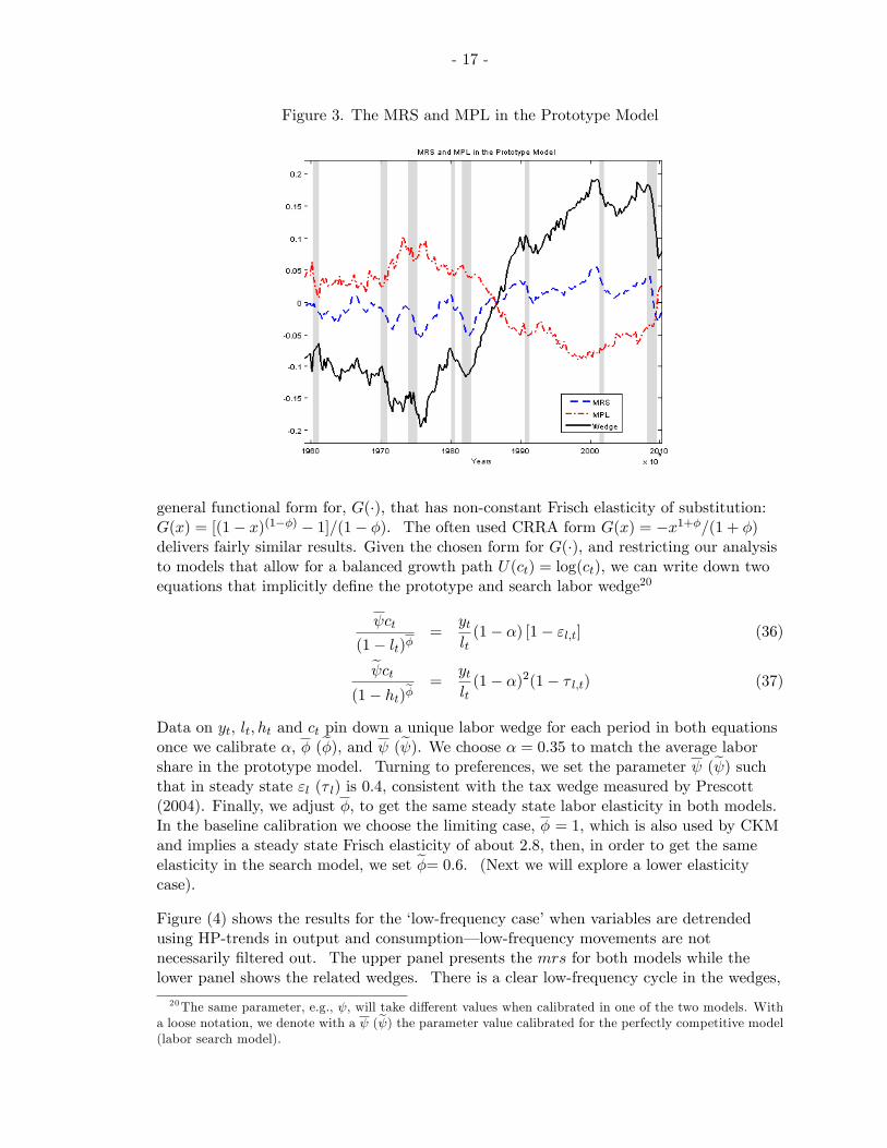
As we mentioned in previous sections, employment fluctuations make the measurement ofthe prototype mrs differ from the one in our search model. This difference is crucial forthe labor wedge, because most of its variation is associated with mrs and not mplfluctuations. Figure (3) plots the log-detrended mrs and mpl jointly with the logdetrended prototype labor wedge. In line with the model, the log mrs, mpl, and [1− εl,t]have been detrended by subtracting the HP-trend of the log of consumption, output, andconsumption-output ratio, respectively (shaded areas indicate NBER recession dates).19

While some low-frequency movements in the labor wedge may be driven by the mpl,particularly between 1982-90, most of the business cycle movements are largely due tofluctuations in the mrs. Hence, seen from the lens of the perfectly competitive model,labor supply is less than implied by the model during expansions and it does not fall asmuch as required by the model during recessions. Given that the search labor wedgedefined in (30) basically modifies the mrs reducing its procyclicality, as we have explainedin the example in (35), the search model points in the right direction.

Quantitative Analysis We recover the labor wedge in the prototype model (theprototype labor wedge) and in the model with labor market search frictions (search laborwedge), from equations (33) and (34), respectively. Conducting this partial accountingexercise requires us to calibrate the disutility of labor, G(·), α, and ψ. We use quite a19The calibration follows strictly the one of CKM. Series are demeaned for ease of comparison.

- 17 -

Figure 3. The MRS and MPL in the Prototype Model

general functional form for, G(·), that has non-constant Frisch elasticity of substitution:G(x) = [(1− x)(1−φ) − 1]/(1− φ). The often used CRRA form G(x) = −x1+φ/(1 + φ)delivers fairly similar results. Given the chosen form for G(·), and restricting our analysisto models that allow for a balanced growth path U(ct) = log(ct), we can write down twoequations that implicitly define the prototype and search labor wedge20

ψct

(1− lt)φ=

ytlt

(1− α) [1− εl,t] (36)

ψct

(1− ht)φ=

ytlt

(1− α)2(1− τ l,t) (37)

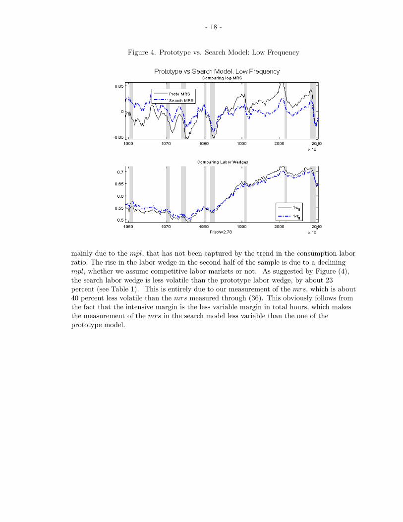
Data on yt, lt, ht and ct pin down a unique labor wedge for each period in both equationsonce we calibrate α, φ (φ), and ψ (ψ). We choose α = 0.35 to match the average laborshare in the prototype model. Turning to preferences, we set the parameter ψ (ψ) suchthat in steady state εl (τ l) is 0.4, consistent with the tax wedge measured by Prescott(2004). Finally, we adjust φ, to get the same steady state labor elasticity in both models.In the baseline calibration we choose the limiting case, φ = 1, which is also used by CKMand implies a steady state Frisch elasticity of about 2.8, then, in order to get the sameelasticity in the search model, we set φ= 0.6. (Next we will explore a lower elasticitycase).

Figure (4) shows the results for the ‘low-frequency case’when variables are detrendedusing HP-trends in output and consumption– low-frequency movements are notnecessarily filtered out. The upper panel presents the mrs for both models while thelower panel shows the related wedges. There is a clear low-frequency cycle in the wedges,

20The same parameter, e.g., ψ, will take different values when calibrated in one of the two models. Witha loose notation, we denote with a ψ (ψ) the parameter value calibrated for the perfectly competitive model(labor search model).

- 18 -

Figure 4. Prototype vs. Search Model: Low Frequency

mainly due to the mpl, that has not been captured by the trend in the consumption-laborratio. The rise in the labor wedge in the second half of the sample is due to a decliningmpl, whether we assume competitive labor markets or not. As suggested by Figure (4),the search labor wedge is less volatile than the prototype labor wedge, by about 23percent (see Table 1). This is entirely due to our measurement of the mrs, which is about40 percent less volatile than the mrs measured through (36). This obviously follows fromthe fact that the intensive margin is the less variable margin in total hours, which makesthe measurement of the mrs in the search model less variable than the one of theprototype model.

- 19 -

Table 1. Moments and Correlations: High Frisch Elasticity

Yt [1− εl,t] [1− τ l,t] mrsprotot mrssearcht

Std. Dev. 0.015 0.015 0.012 0.013 0.010(0.015) (0.074) (0.057) (0.024) (0.014)

Corr(xt, xt−1) 0.862 0.749 0.666 0.893 0.865(0.862) (0.988) (0.983) (0.966) (0.922)

Cross CorrelationsYt Lt C/Y

[1− εl,t] 0.514 0.866 −0.162(0.183) (0.992) (−0.086)

[1− τ l,t] 0.410 0.796 −0.043(0.173) (0.978) (−0.066)

All variables are HP-filtered, except Lt.Moments in () are for the ‘low-frequency’case.

As shown in Table 1 the correlations of the labor wedge with cyclical variables aresubstantially different from zero (excluding the consumption-output ratio). Results areparticularly evident at business cycle frequency– in this case each variable in Table 1, butLt, has been HP-filtered (shown in Figure 5). Given a relatively high Frisch elasticity(about 2.78), at business cycle frequency the search labor wedge is 20 percent less volatilethan the prototype wedge (see Table 1). As in the low-frequency case, the nature of thedecline stems from the measurement of the mrs. Moreover, the correlation with totalhours is reduced by about 8 percent while the one with output by 20 percent.

While the calibration of α and ψ has no implication for our analysis, results are clearlyaffected by the choice of the parameter that governs the Frisch elasticity φ. So far, theFrisch elasticity we have used in the numerical exercises was 2.78, in line with most macromodel and chosen to be comparable with CKM. However, this elasticity is at high end ofthe estimates found in the micro literature (Blundell and MaCurdy 1999). In what followswe will show that our results are indeed amplified when the Frisch elasticity is chosenconsistent with most of the micro estimates.

Low Frisch Elasticity The major problem behind the failure of the prototype model,as well as our extension of it, is that hours do not vary as much in the data as implied byour models. This has been well-recognized in the context of macro models. Higheraggregate micro elasticities tend to produce smaller wedges at the expense of a large microliterature that argues for lower individual labor elasticities. Here, we replicate ourexercise by targeting a Frisch elasticity of 0.5 on average, which is more in line with thesestudies. Figures (6), (7) and Table 2 present our results.21

While the overall volatility is higher across variables, there is a dramatic reduction in the

21This requires φ = 5.54 in (36) and φ = 3.33 in (37) for the given sample averages of L and h.

- 20 -

Figure 5. Prototype vs. Search Model: Business Cycle Frequency

Figure 6. Prototype vs. Search Model: Low Frequancy and low Frisch Elasticity

- 21 -

Figure 7. Prototype vs. Search Model: Business Cycle Frequency and Low Frisch Elasticity

volatility of the labor wedge with search frictions of more than 40 percent, both at lowfrequency (Figure 6) and at business cycle frequency (Figure 7). Once again, thisreduction is entirely due to the lower volatility in mrs as measured by our model. Thereduction in correlation with output is about 22 percent at business cycle frequency. Notehowever, that a lower Frisch elasticity increases the overall standard deviation in bothwedges relative to high elasticity case. Given that wages are not very volatile in the data,most macro models favor a high elasticity. However, while in the prototype model thevolatility of the mrs triples, the mrs volatility in the low elasticity case is only 1.46 timesthe one in the prototype high elasticity case, which makes the labor search model muchmore promising in reconciling micro and macro estimates.

- 22 -

Table 2. Moments and Correlations: Low Frisch Elasticity

Yt [1− εl,t] [1− τ l,t] mrsprotot mrssearcht

Std. Dev. 0.015 0.037 0.021 0.035 0.019(0.015) (0.165) (0.082) (0.114) (0.052)

Corr(xt, xt−1) 0.862 0.818 0.59 0.875 0.732(0.862) (0.99) (0.971) (0.987) (0.962)

Cross CorrelationsYt Lt C/Y

[1− εl,t] 0.721 0.975 -0.452(0.238) (0.998) (−0.153)

(1− τ l,t) 0.56 0.869 -0.283(0.229) (0.813) (−0.132)

All variables are HP-filtered, except Lt.Moments in () are for the ‘low-frequency’case.

Our comparison between the statistical properties of the two wedges, so far points to apotential misspecification in the prototype model. We can argue that an econometricianmeasuring the labor wedge based on (36) might misinterpret some endogenous variation inhours as variation in the labor wedge.

B. Mapping with the simulated data

The previous section has analyzed the labor wedge based solely on one equilibriumcondition. In this section, instead, we use the model as the data generating process andanalyze what it implies for the labor wedge of the prototype RBC model. Morespecifically, we calibrate our model and simulate artificial data by shutting off all theexogenous shocks (and wedges) except the effi ciency wedge, Zt, which means that [1− τ l,t]will be constant at 0.6 over time. Then, using the simulated data on consumption,output and labor, we measure a labor wedge as in CKM using (36). Hence, the nullhypothesis is no movements in the prototype labor wedge, i.e., εl,t = .4 ∀t.

To calibrate parameters related to search frictions we follow an approach that is similar toMerz (1995) and Andolfatto (1996), and target first moments of the labor marketvariables, n and h. We follow a standard approach for parameters that are not related tosearch frictions. More specifically, we set β = 0.99, δ = 0.025, α = 0.36. Note that 1− αis not equal to labor’s share because of the search frictions, but as long as the totalrecruiting costs is a relatively small fraction of output, labor’s share is not far from 1− α.The total recruiting cost share, i.e. κv/y, is set to 1.5 percent. We follow Merz (1995) andassume a strictly convex search cost function c(e) = c0e

µ, where c0 is normalized to 1 andthe output share of search costs born by workers, c(e)(1− n), is targeted to be 0.5 percent.Unfortunately, there is no guidance in the literature over these parameters and we try tominimize the resource cost of search and recruitment by this calibration. It turns out thisis not far from what has been done in the literature before and our results are notsensitive to the exact share of these costs (see Andolfatto 1996). What is more sensitive is

- 23 -

the parameter µ, that determines the degree of convexity in cost of worker’s search effort.As we have argued in section 4.4, in order to have a unique steady state equilibrium weneed to have enough convexity in this function. In particular, as µ converges to 1 we willhave multiplicity of equilibria. In our calibration µ is implied by the relative ratios of thesearch/recruitment costs in output, i.e. µ = 3.22 The elasticity of matching function andbargaining power of workers (firms) are calibrated such that the Hosios (1990) conditionholds, which implies γ = λ. The elasticity of job matches with respect to vacancies, γ, isset to 0.5, which lies in the middle of the range of estimates reported by Petrongolo andPissarides (2001). The quarterly rate of transition from employment to non-employment,σ, is set at 0.15, following calibration of Andolfatto (1996) and references therein. Fiveparameters, µ, φ, ψ, κ and χ are calibrated to match five moments, κv/y = 0.015,c(e)(1− n)/y = 0.005, n = 0.7074, h = 0.3752, and q = 0.9.23

Figure 8. Simulated Data: Labor Wedge and Output .

20 40 60 80 100 120 140 160 180 200

­4

­3

­2

­1

0

1

2

3

4

5

quarters

log­

devi

atio

ns

Simulated Series: Labor Wedge vs. Output

Lab. WedgeOutput

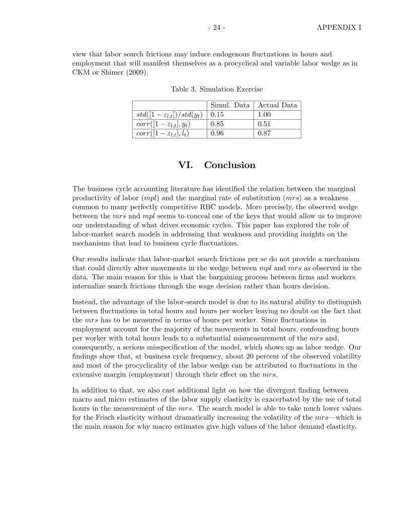
Figure (8) shows simulated output series and the prototype labor wedge derived under thebaseline calibration described above. The standard deviation of εLt relative to output is0.15 which makes the null hypothesis of no fluctuations clearly rejected. In other words,this implies that doing the business cycle accounting as in CKM would falsely detect thepresence of a labor wedge when reality is well described by the labor search model.Moreover, the correlation between the labor wedge is strongly procyclical with acorrelation with output and total hours of about 0.85 and 0.96, respectively. Hence, asimple extension of the prototype RBC model with search frictions is consistent with asignificantly procyclical labor wedge, which could be entirely due to endogenousmovements in both the extensive and the intensive margins. Those results support the

22Our results are essentially same when µ = 1.5.23Note that, in this quantitative exercise, shocks to the matching effi ciency is shut down, as well as τ l and

g,. The latter two parameters are set to 2/5 and 0.16, respectively, following the avergaes in the data andthe measured labor wedge from the previous section. Our targets for n and h are the means for employmentand hours per worker respectively. The calibration target for q follows from the average duration of a postedvacancy based on van Ours and Ridder (1992).

- 24 - APPENDIX I

view that labor search frictions may induce endogenous fluctuations in hours andemployment that will manifest themselves as a procyclical and variable labor wedge as inCKM or Shimer (2009).

Table 3. Simulation Exercise

Simul. Data Actual Datastd([1− εl,t])/std(yt) 0.15 1.00corr([1− εl,t], yt) 0.85 0.51corr([1− εl,t], lt) 0.96 0.87

VI. Conclusion

The business cycle accounting literature has identified the relation between the marginalproductivity of labor (mpl) and the marginal rate of substitution (mrs) as a weaknesscommon to many perfectly competitive RBC models. More precisely, the observed wedgebetween the mrs and mpl seems to conceal one of the keys that would allow us to improveour understanding of what drives economic cycles. This paper has explored the role oflabor-market search models in addressing that weakness and providing insights on themechanisms that lead to business cycle fluctuations.

Our results indicate that labor-market search frictions per se do not provide a mechanismthat could directly alter movements in the wedge between mpl and mrs as observed in thedata. The main reason for this is that the bargaining process between firms and workersinternalize search frictions through the wage decision rather than hours decision.

Instead, the advantage of the labor-search model is due to its natural ability to distinguishbetween fluctuations in total hours and hours per worker leaving no doubt on the fact thatthe mrs has to be measured in terms of hours per worker. Since fluctuations inemployment account for the majority of the movements in total hours, confounding hoursper worker with total hours leads to a substantial mismeasurement of the mrs and,consequently, a serious misspecification of the model, which shows up as labor wedge. Ourfindings show that, at business cycle frequency, about 20 percent of the observed volatilityand most of the procyclicality of the labor wedge can be attributed to fluctuations in theextensive margin (employment) through their effect on the mrs.

In addition to that, we also cast additional light on how the divergent finding betweenmacro and micro estimates of the labor supply elasticity is exacerbated by the use of totalhours in the measurement of the mrs. The search model is able to take much lower valuesfor the Frisch elasticity without dramatically increasing the volatility of the mrs– which isthe main reason for why macro estimates give high values of the labor demand elasticity.

- 25 - APPENDIX II

Appendices

Appendix 1

Data

We use data from NIPA tables to construct our measures for real output (yt),consumption (ct), and government expenditures (εg,t), which also includes net exports24.Labor market variables, employment (nt) and average hours per worker (ht) are takenfrom Cociuba, Prescott and Ueberfeldt (2009). All the data are from 1959:Q2 to through2010:Q3 and seasonally adjusted at an annualized rate when relevant. Output, yt,andsome of its components,ct , and εg,t are all deflated by the GDP deflator. Real output, ytis defined as the quarterly gross domestic product net of sales taxes. Consumption, ct, isthe sum of non-durable goods purchases and services. Finally, government expenditures,εg,t, includes government consumption expenditures (including federal, state and localgovernments) and net exports of goods and services. In effect we lump togethergovernment consumption and net exports. For the purpose of our exercises in this paperthis distinction is not important. For the labor market data, we follow Cociuba, Prescottand Ueberfeldt (2009) and use their data to incorporate military hours and employmentinto total hours and total employment figures as estimated by the Current PopulationSurvey of the BLS.

Appendix 2

Households’Decision Problem

First order necessary conditions and costates for the household’s problem (15)-(16) are,

xt : −Uc(ct) [1 + τx,t] + βEtW hkt+1(ω

ht+1|ωht )

∂kt+1∂xt

= 0 (38)

et : −Uc(ct)ce(et)(1− nt) + βEtW hnt+1(ω

ht+1|ωht )

∂nt+1∂et

= 0 (39)

kt : W hkt(ω

ht |ωht−1) = Uc(ct)rt + βEtW h

kt+1(ωht+1|ωht )

∂kt+1∂kt

(40)

nt : W hnt(ω

ht |ωht−1) = Uc(ct)[wt [1− τ l,t]ht + c(et)] + ψG(ht) + βEtW h

nt+1(ωht+1|ωht )

∂nt+1∂nt

.(41)

Combining (38) and (40) will give the consumption Euler equation in (17). Note that

equation (39) implies that βEtW hnt+1(ω

ht+1|ωht ) =

Uct (ct)cet (et)pt

. Substituting this expression

for βEtW hnt+1(ω

ht+1|ωht ) in (41) and taking expectations using (39) gives the households’

choice of effort in (18).

24We pulled this data from Haver Analytics database.

- 26 -

Firms’Decision Problem

First order necessary conditions and costates for the firms’problem (19)-(20) are,

kt : τ z,tfk(kt, ntht)− rt = 0 (42)

vt : −κ+ qtβEtW f (ωft+1|ωft ) = 0 (43)

kt+1 : W fnt(ω

ft |ω

ft−1) = τ z,tfk(kt, ntht)ht − wtht + (1− σ)βtEtW

fnt+1(ω

ft |ω

ft−1) (44)

Equation (42) gives us the equilibrium rental rate on capital in (21). Note that equation(43) implies that βtEtW

fnt+1(ω

ft+1|ω

ft ) = κ

qt. Substituting this expression for

βtEtWf (ωft+1|ω

ft ) in (44) and taking expectations using (42) gives the firms’choice of

vacancies in (22).

Details of Employment Contract

Employment contract is given by the solution to the problem defined in (23). Note thatwe have the necessary expressions for each party’s marginal surplus from respectivedecision problems. W h

nt(ωt) is defined in (41) and Wfnt(ωt) is defined in (44).

W hnt(ω

ht ) = Uc(ct)[wt [1− τ l,t]ht + c(e)] + ψG(ht) + (1− σ − pte)βEtW h

nt+1(ωht+1|ωht )(45)

W fnt(ω

ft ) = τ z,tflt(kt, ntht)ht − wtht + (1− σ) βtEtW

fnt+1(ω

ft+1|ω

ft ) (46)

As long as there are gains from trade, first order conditions are given by two conditionsthat determine optimal hours and wage.

wt : λW fnw(ωft )

W fn (ωft )

+ (1− λ)W hnw(ωht )

W hn (ωht )

= 0

ht : λW fnh(ωft )

W fn (ωft )

+ (1− λ)W hnh(ωht )

W hn (ωht )

= 0

where the cross-partial derivatives could be evaluated by using (45) and (46) to arrive at(24) and (25) in the text. Then one can use the wage equation, (24), along with (45) and(46) to derive an explicit wage equation in (26). To do so, multiply both sides of (45)with λ and (46) with (1− λ)Uc(ct) [1− τ l,t].

λW hn (ωht ) = λUc(ct)[wt [1− τ lt]ht + c(e)] +

λψG(ht) + λ (1− σ − pte)βEtW hn (ωht+1|ωht )

(1− λ)Uc(ct) [1− τ lt ]W fn (ωft ) = (1− λ)Uc(ct) [1− τ l,t] [εz,tfl(kt, ntht)ht − wtht]

+(1− λ)Uc(ct) [1− τ l,t] (1− σ) βtEtWfn (ωft+1|ω

ft )

Substituting for βEtW hnt+1(ω

ht+1|ωht ) and βEtW

fnt+1(ω

ft+1|ω

ft ) and subtracting the second

line from the first with some additional algebra gives the wage equation expressed in (26).Finally, it is straightforward to see that the optimality in hours from Nash bargainingproblem implies the labor wedge equation expressed in (30).

- 27 -

References

Andolfatto, David. 1996. “Business Cycles and Labor Market Search.”AmericanEconomic Review, 86(1): 112—132.

Arseneau, David M., and Sanjay K. Chugh. 2010. “Tax Smoothing in Frcitional LaborMarkets.”mimeo. Board of Governors of the Federal Reserve.System

Beuchemin Kenneth, and Murat Tasci. 2008. “Diagnosing Labor Market Search Models:A Multiple-Shock Approach.”Working Paper. Federal Reserve Bank of Cleveland.

Blanchard, Olivier Jean, and Jordi Gali. 2010. “Labor Markets and Monetary Policy: ANew Keynesian Model with Unemployment.”American Economic Journal:Macroeconomics, 2: 1—30.

Blundell, Richard and Thomas MaCurdy. 1999. “Labor Supply: A review of alternativeapproaches.” in Handbook of Labor Economics, ed. Orley C. Ashenfelter and DavidCard, 1559—1695. Amsterdam: North-Holland.

Chari, V.V., Patrick Kehoe, and Ellen R. McGratten. 2007. "Business CycleAccounting.”Econometrica, 75(3): 781-836.

Chang, Yongsung, and Sun-Bin Kim. 2007. “Heterogeneity and Aggregation: Implicationsfor Labor Market Fluctuations.”American Economic Review, 97(5): 1939—1956.

Cheremukhin, Anton A., and Paulina Restrepo-Echavarria. 2010. “The Labor Wedge as aMatching Friction.”Working Paper #1004. Federal Reserve Bank of Dallas.

Cociuba, Simona., Alexander Ueberfeldt and Edward C. Prescott. 2009. “U.S. Hours andProductivity Behavior Using CPS Hours Worked Data: 1947-III to 2009-II.”Mimeo.Federal Reserve Bank of Dallas.

Cociuba, Simona, and Alexander Ueberfeldt. 2010. “Trends in U.S. Hours and the LaborWedge.”Mimeo. Federal Reserve Bank of Dallas.

Cole, Harold L., and Richard Rogerson. 1999. “Can the Mortensen-Pissarides Matchingmodel Match the Business Cycle Facts?”International Economic Review, 40(4):933-959.

Cole, Harold L., and Lee E. Ohanian. 2002. “The U.S. and U.K. Great Depressionsthrough the Lens of Neoclassical Growth Theory”American Economic Review:Papers and Proceedings, 92 (2): 28—32.

Elsby, Michael, Ryan Michaels. 2010. “Marginal Jobs, Heterogenous Firms, andUnemployment Flows.”Working Paper. University of Michigan.

Fujita, Shigeru and Makoto Nakajima. 2009. “Worker Flows and Job Flows: AQuantitative Investigation.”Working Paper #09-33. Federal Reserve Bank ofPhiladelphia.

- 28 -

Gali, Jordi, Mark Gertler, and J. David Lopez-Salido. 2007. “Markups, Gaps, and theWelfare Costs of Business Fluctuations.”Review of Economics and Statistics, 89(1):44—59.

Hall, Robert E. 1997. “Macroeconomic Fluctuations and the Allocation of Time.”Journal of Labor Economics, 15(1): 223—250.

Hosios, A. 1990. “On the Effi ciency of Matching and Related Models of Search andUnemployment.”Review of Economic Studies, 57(2): 279—298.

Kydland Finn E., and Edward J. Prescott. 1982. "Time to Build and AggregateFluctuations.”Econometrica, 50(6): 1345-1370.

Ingram, B. F., Narayana Kocherlakota and N. Eugene Savin. 1994. “Explaining BusinessCycles: A multiple-shock approach.”Journal of Monetary Economics, 34(3):415—428.

Merz, Monika. 1995. “Search in the Labor Market and the Real Business Cycle.”Journalof Monetary Economics, 36(2): 269—300.

Merz, Monika. 1999. "Heterogeneous Job-Matches and the Cyclical Behavior of LaborTurnover." Journal of Monetary Economics, 43(1): 91-124.

Mortensen, Dale and Christopher A. Pissarides. 1994. “Job Creation and Job Destructionin the Theory of Unemployment.”Review of Economic Studies, 61(3): 397—415.

Mulligan, Casey B. 2002. “A Century of Labor-Leisure Distortions.”Working Paper8774, National Bureau of Economic Research.

Ohanian, Lee E., Richard Rogerson and Andrea Raffo. 2008. “Long-Term Changes inLabor Supply and Taxes: Evidence from OECD Countries, 1956-2004.”Journal ofMonetary Economics, 55(8): 1353—1362.

Petrongolo, Barbara and Christopher A. Pissarides. 2001. “Looking into the Black Box:A Survey of the Matching Function.”Journal of Economic Literature, 39(2):390—431.

Pissarides, Christopher A. 2000. Equilibrium Unemployment Theory. Cambridge: MITPress.

Prescott, Edward J. 1986. “Theory Ahead of Business Cycle Measurement.”FederalReserve Bank of Minneapolis Quarterly Review, 10: 9—22.

Prescott, Edward J. 2004. “Why Do Americans Work So Much More Than Europeans?”Federal Reserve Bank of Minneapolis Quarterly Review, 28: 2—13.

Rotemberg, Julio J. and Michael Woodford. 1991. “Markups and the Business Cycle.”NBER Macroeconomics Annual, 6: 63—129.

Rotemberg, Julio J. and Michael Woodford. 1999. “The Cyclical Behavior of Prices and

- 29 -

Costs.” in Handbook of Macroeconomics, ed. John Taylor and Michael Woodford,1051—1135. Amsterdam: North-Holland.

Shimer, Robert. 2005. “The Cyclical Behavior of Unemployment and Vacancies:Evidence and Theory.”American Economic Review. 95(1): 25-49.

Shimer, Robert. 2009. “Convergence in Macroeconomics: The Labor Wedge.”AmericanEconomic Journal: Macroeconomics, 1(1): 280—297.

Shimer, Robert. 2010. Labor Markets and Business Cycles. Princeton: PrincetonUniversity Press.

Stole, Lars A. and Jeffrey Zwiebel. 1996. “Inrafirm Bargaining under Non-bindingContracts”Review of Economic Studies, 63(3): 375—410.

van Ours, Jan C., and Geert Ridder. 1992. “Vacancies and the Recruitment of NewEmployees.”Journal of Labor Economics, 10(2): 138—155.