"School Nutrition Programs and the Incidence of … · School Nutrition Programs and the Incidence...
36
NBER WORKING PAPER SERIES SCHOOL NUTRITION PROGRAMS AND THE INCIDENCE OF CHILDHOOD OBESITY Daniel L. Millimet Rusty Tchernis Muna Husain Working Paper 14297 http://www.nber.org/papers/w14297 NATIONAL BUREAU OF ECONOMIC RESEARCH 1050 Massachusetts Avenue Cambridge, MA 02138 September 2008 The authors wish to thank Patricia Anderson, Steven Haider, Elaina Rose, Jayjit Roy, seminar participants at Georgetown University Public Policy Institute, Texas Camp Econometrics, and conference participants at the Western Economic Association International Annual Meetings. The views expressed herein are those of the author(s) and do not necessarily reflect the views of the National Bureau of Economic Research. NBER working papers are circulated for discussion and comment purposes. They have not been peer- reviewed or been subject to the review by the NBER Board of Directors that accompanies official NBER publications. © 2008 by Daniel L. Millimet, Rusty Tchernis, and Muna Husain. All rights reserved. Short sections of text, not to exceed two paragraphs, may be quoted without explicit permission provided that full credit, including © notice, is given to the source.
Transcript of "School Nutrition Programs and the Incidence of … · School Nutrition Programs and the Incidence...

NBER WORKING PAPER SERIES
SCHOOL NUTRITION PROGRAMS AND THE INCIDENCE OF CHILDHOODOBESITY
Daniel L. MillimetRusty TchernisMuna Husain
Working Paper 14297http://www.nber.org/papers/w14297
NATIONAL BUREAU OF ECONOMIC RESEARCH1050 Massachusetts Avenue
Cambridge, MA 02138September 2008
The authors wish to thank Patricia Anderson, Steven Haider, Elaina Rose, Jayjit Roy, seminar participantsat Georgetown University Public Policy Institute, Texas Camp Econometrics, and conference participantsat the Western Economic Association International Annual Meetings. The views expressed hereinare those of the author(s) and do not necessarily reflect the views of the National Bureau of EconomicResearch.
NBER working papers are circulated for discussion and comment purposes. They have not been peer-reviewed or been subject to the review by the NBER Board of Directors that accompanies officialNBER publications.
© 2008 by Daniel L. Millimet, Rusty Tchernis, and Muna Husain. All rights reserved. Short sectionsof text, not to exceed two paragraphs, may be quoted without explicit permission provided that fullcredit, including © notice, is given to the source.

School Nutrition Programs and the Incidence of Childhood ObesityDaniel L. Millimet, Rusty Tchernis, and Muna HusainNBER Working Paper No. 14297September 2008JEL No. C13,H51,I18,I28
ABSTRACT
In light of the recent rise in childhood obesity, the School Breakfast Program (SBP) and National SchoolLunch Program (NSLP) have received renewed attention. Using panel data on over 13,500 primaryschool students, we assess the relationship between SBP and NSLP participation and (relatively) long-runmeasures of child weight. After documenting a positive association between SBP participation andchild weight, and no association between NSLP participation and child weight, we present evidenceindicating positive selection into the SBP. Allowing for even modest positive selection is sufficientto alter the results, indicating that the SBP is a valuable tool in the current battle against childhoodobesity, whereas the NSLP exacerbates the current epidemic.
Daniel L. MillimetSouthern Methodist UniversityDepartment of EconomicsBox 0496Dallas, TX [email protected]
Rusty TchernisDepartment of EconomicsIndiana UniversityWylie Hall 105100 South WoodlawnBloomington, IN 47405and [email protected]
Muna HusainSMU, Department of EconomicsBox 0496Dallas, TX [email protected]

1 Introduction
As is quite evident from recent media reports, childhood obesity is deemed to have reached epidemic
status. Data from the National Health and Nutrition Examination Survey (NHANES) I (1971�1974) and
NHANES 2003�2004 indicate that the prevalence of overweight preschool-aged children, aged 2-5 years,
increased from 5.0% to 13.9% over this time period.1 Among school-aged children, the prevalence has risen
from 4.0% to 18.8% for those aged 6-11; 6.1% to 17.4% for those aged 12-19 years.2
Given this backdrop, policymakers in the US have acted in a number of di¤erent directions, particularly
within schools. Public Law 108-265 requires schools to have a local wellness program by the beginning of the
2006-2007 school year, which must address both nutritional and physical activity goals. The CDC started
the KidsWalk-to-School Program to encourage communities to partner with parents and local public safety
o¢ cials to enable students to safely walk or bicycle to school in groups accompanied by adults. Some schools
have banned soda machines and vending machines containing unhealthy snacks, while others have taken
aggressive measures to ensure the provision of nutritious meals.3 Texas reinstated a physical education
requirement, which had been previously removed in favor of more academic pursuits (Schanzenbach 2007).
In November 2007, the US Department of Health and Human Services (HHS) launched the Childhood
Overweight and Obesity Prevention Initiative.
Aside from these recent policy developments, two federal programs that have long been in existence
have been met with renewed interest: the School Breakfast Program (SBP) and the National School Lunch
Program (NSLP). Given the number of children a¤ected and potentially a¤ected by these programs, com-
bined with the fact that the infrastructure for these programs is already in existence, it is the relationship
between the SBP, NSLP, and child weight that we analyze here. Speci�cally, we have three main objec-
tives. First, assess the relatively long-run relationship between participation in school nutrition programs
and child weight using data collected after the most recent, large-scale reforms of the programs. Second,
analyze the process by which children select into the SBP and NSLP. Finally, assess the impact of such
selection on our ability to infer a causal relationship.
Understanding the relationship between school nutrition programs and child weight is clearly impor-
tant. As the incidence of overweight children has increased, so too has our understanding of the negative
consequences that result. First and foremost, overweight children are signi�cantly more likely to become
obese adults. Serdula et al. (1993) �nd that one-third of overweight preschool-aged children and one-half of
1Overweight is de�ned as an age- and gender-speci�c body mass index (BMI) greater than the 95th percentile based on
growth charts from the Center for Disease Control (CDC).2See http://www.cdc.gov/nccdphp/dnpa/obesity/childhood/prevalence.htm.3Andersen and Butcher (2006) �nd that the elasticity of BMI with respect to junk food exposure in schools is roughly 0.1.
1
overweight school-aged children become obese adults. Second, the adverse health e¤ects of obesity include,
among others, depression, sleep disorders, asthma, cardiovascular and pulmonary complications, and type
II diabetes (Ebbling et al. 2002). In terms of economic costs, Finkelstein et al. (2003) report that medical
spending attributed to obesity was close to $80 billion, or 9% of total medical expenditures, in the US in
1998. Bleich et al. (2007) provide a recent overview of the costs and consequences of adult obesity.
In this study, we utilize panel data on over 13,500 children during early primary school to examine
the relatively long-run e¤ect of participation in both the SBP and NSLP. Speci�cally, we analyze the
relationship between child weight in the spring of third grade and program participation in spring of
kindergarten. Analyzing the long-run impact allows us to capture dynamic e¤ects of program participation
such as nutritional habit formation and resource reallocation within households. In addition, after assessing
the nature of selection into both programs, we examine the sensitivity of the estimated program e¤ects to
non-random selection, borrowing several methods from the program evaluation literature.
Our results are striking, yielding three salient �ndings. First, while SBP participation in kindergarten
is associated with greater child weight in third grade and a greater change in child weight between kinder-
garten and third grade for many children, NSLP participation and child weight are unrelated. However,
we �nd strong evidence of non-random selection into the SBP; children who gained more weight prior
to kindergarten are more likely to participate. Consonant with Schanzenbach (2007), selection bias does
not seem to be a concern when analyzing the NSLP. Finally, in nearly all cases, the positive associations
between SBP participation and child weight are found to be extremely sensitive to non-random selection;
even a modest amount of positive selection is su¢ cient to eliminate, if not reverse, the initial results for
SBP. Moreover, allowing for modest positive selection into the SBP leads to a detrimental e¤ect of NSLP
participation on child weight; ignoring non-random selection into SBP biases the impact of the NSLP
toward zero. Thus, admitting even modest positive selection into the SBP implies that the SBP is a
valuable tool in the current battle against childhood obesity, whereas the NSLP exacerbates the current
epidemic. The bene�cial e¤ect of the SBP, and the deleterious impact of the NSLP, strengthen the �ndings
in Bhattacharya et al. (2006) and Schanzenbach (2007), respectively.
The remainder of the paper is organized as follows. Section 2 provides background information, both
on the school nutrition programs themselves, as well as the previous literature. Section 3 presents a simple
theoretical framework for thinking about school nutrition programs. Section 4 describes the empirical
methodology and the data. Section 5 presents the results, while Section 6 concludes.
2

2 Background
2.1 Institutional Details
The NSLP was developed gradually, and made permanent by the National School Lunch Act in 1946. The
program provides lunch to over 29 million children each school day, covering approximately 99,000 schools
(95% of all public and private schools), with 17.5 million students receiving reduced price or free meals.4
The SBP was established in 1966 by the Child Nutrition Act, and made permanent in 1975. During the
2005-2006 school year, the SBP provided breakfast to roughly 9.6 million children in 82,000 schools, with
7.7 million children receiving reduced price or free breakfasts (Cooper and Levin 2006).
As evidenced by these �gures, the SBP is under-utilized relative to the NSLP. Roughly 83% of schools
participating in the NSLP also participated in the SBP during the 2005-2006 school year, and roughly
45 students qualifying for free or reduced price meals participated in the SBP for every 100 students
participating in the NSLP (Cooper and Levin 2006). That said, SBP participation is on the rise, having
increased in all but three states from the 2004-2005 school year to the 2005-2006 school year.
The SBP and NSLP are similarly organized. Both programs are federally funded. Each is overseen by
the Food and Nutrition Service (FNS) of the US Department of Agriculture (USDA), but administered
by state education agencies. Schools deciding to participate in the programs must o¤er meals that meet
federal nutritional requirements. In addition, students residing in households with family incomes at or
below 130% of the federal poverty line are eligible for free meals, while those in households with family
incomes between 130% and 185% of the federal poverty line are entitled to reduced price meals.5 Eligible
children apply directly to the school, with the same application covering both the SBP and NSLP. In
addition, children from households that receive aid through food stamps, Temporary Assistance for Needy
Families, or the Food Distribution Program on Indian Reservations are automatically eligible for free meals.
All other students pay full price, though meals are subsidized by the federal government to a limited extent.
Schools establish their own prices for full price meals, but prices for reduced price meals are capped.
Schools have �exibility with respect to the speci�c foods served, but are constrained by the fact they
must operate their meal services as non-pro�t programs. In the 2005 �scal year, the NSLP cost the federal
government roughly $7 billion, while federal expenditures on the SBP in �scal year 2006 totalled $2 billion.6
As stated above, reimbursement is conditional on the meals meeting federal nutritional requirements,
established by Congress in 1995 under the �School Meals Initiative for Healthy Children� (SMI). SMI
4See http://www.fns.usda.gov/cnd/lunch/AboutLunch/NSLPFactSheet.pdf.5For the period July 1, 2007, through June 30, 2008, 130% (185%) of the federal poverty line for a family of four is $26,845
($38,203). The maximum price allowed for breakfast (lunch) to students qualifying for reduced price is $0.30 ($0.40).6See http://www.frac.org/pdf/cnnslp.PDF and http://www.frac.org/pdf/cnsbp.PDF.
3

represented the largest reform of the programs since their inception (Lutz et al. 1999). For breakfast, this
entails no more than 30% of the meal�s calories be derived from fat, and less than 10% from saturated
fat. Breakfasts also must provide one-fourth of the Recommended Dietary Allowance (RDA) for protein,
calcium, iron, Vitamin A, Vitamin C, and contain an age-appropriate level of calories. For lunches, the
same restrictions on fat apply. However, lunches must provide one-third of the RDA for protein, calcium,
iron, Vitamin A, Vitamin C, and an age-appropriate level of calories calories. In addition, all meals are
recommended to reduce levels of sodium and cholesterol, as well as increase the level of dietary �ber.
Enforcement of the SMI requirements is handled by requiring states to monitor local school food
authorities through reviews conducted at least once every �ve years. In turn, the FNS monitors state
compliance with this review requirement. The FNS has also begun to provide regional and local training
to ensure adequate overview.
2.2 Literature Review
Given the size and cost of these programs, each has been studied to some extent over the decades. In
the early 1990s, a series of studies were conducted utilizing the 1992 School Nutrition Dietary Assessment
(SNDA-1) study. As part of the study, a random sample of school meals was analyzed, in addition to the
diets of children. Gleason (1995) �nds that SBP availability is not associated with a higher probability of
eating breakfast. Moreover, the author �nds that lunches provided under the NSLP derived an average
of 38% of food energy from fat, exceeding guidelines. Burghardt et al. (1995) report that meals provided
under the NSLP exceeded guidelines for total and saturated fat and sodium, whereas meals provided under
the SBP exceeded guidelines for saturated fat and cholesterol. Gordon et al. (1995) use 24-hour dietary
recall data and conclude that both SBP and NSLP participation are associated with higher intake of fat
and saturated fat, but also some nutrients.
The results of the analyses using the SNDA-1 led to the 1995 SMI discussed above. While the SMI
required schools to follow the nutrition guidelines by the 1996-1997 school year, some schools received a
waiver until the 1998-1999 school year (Lutz et al. 1999). A second study, the SNDA-2, was conducted in
1998-1999. The evidence suggests some e¤ect of the SMI on the nutritional content of meals, but school
lunches in particular still have much room for improvement (Schanzenbach 2007).7
Since the SNDA-1 study, more recent analyses have focused greater attention on identifying the causal
impact of SBP or NSLP participation on child health. Gleason and Suitor (2003) use two nonconsecutive
days of 24-hour dietary recall data to obtain �xed e¤ects estimates of NSLP participation. The authors
�nd that NSLP participation increases intake of nutrients, but also increases intake of dietary fat. Ho¤erth
7See also http://www.iom.edu/Object.File/Master/31/064/Jay%20Hirschman.IOM%20Presentation.Oct%2026%202005.pdf.
4

and Curtin (2005) use data from the 1997 Child Development Supplement of the Panel Study for Income
Dynamics (PSID) and �nd no e¤ect of SBP participation on the probability of being overweight after
controlling for NSLP participation. In addition, instrumental variables estimates � using public school
attendance as the exclusion restriction � indicate no impact of NSLP participation. Bhattacharya et
al. (2006) analyze the e¤ects of SBP availability in the school on nutritional intake using NHANES III,
which spans 1988-1994 (thus pre-dating the SMI). The authors employ a di¤erence-in-di¤erences strategy
(comparing in-school versus out-of-school periods in schools participating and not participating in the
SBP), concluding that SBP availability �has no e¤ect on the total number of calories consumed or on the
probability that a child eats breakfast, but it improves the nutritional quality of the diet substantially�(p.
447). Schanzenbach (2007) utilizes panel data methods, as well as a regression discontinuity (RD) approach
that exploits the sharp income cut-o¤ for eligibility for reduced-price meals, to assess the impact of the
NSLP. Using data from the Early Childhood Longitudinal Study-Kindergarten Class of 1998-99 (ECLS-K),
she �nds that NSLP participation increases the probability of being obese due to the additional calories
provided by school lunches. However, she �nds little substantive di¤erence between the RD estimates and
those based on a panel data approach, suggesting little selection into the NSLP on the basis of unobservables
that vary over time and across schools.
Finally, a few studies o¤er less direct evidence of the possible e¤ects of the SBP and NSLP. For
instance, Long (1991) assesses the crowding-out impact of SBP and NSLP bene�ts on total household
food expenditures. The author �nds that one dollar of NSLP (SBP) bene�ts displaces only $0.60 (none)
of household food expenditures. Thus, both programs increase the total value of food consumed by the
household. von Hippel et al. (2007) show that children are more at-risk of gaining weight during summer
vacation than during the school-year. While this is potentially attributable to children�s propensity to
consume more food while at home, it could also be explained by the lack of access to school meal programs
during the summer for non-summer school attendees.
We add to this literature in four important ways. First, we assess the long-run relationship between
participation in both the SBP and NSLP program and children�s weight. Second, we use data after the
reforms enacted under the SMI should have been fully implemented. Most prior research (to our knowledge)
assesses the contemporaneous relationship between SBP and/or NSLP participation and children�s weight,
typically focuses on only one of the programs (not both), and uses data from before the changes instituted
under the SMI have been fully implemented. Third, we assess the nature of selection into both programs
using data on birthweight and weight at the time of entry into kindergarten. Finally, we examine the
sensitivity of the estimated program e¤ects to non-random selection.
5

3 Theoretical Motivation
To provide some context for the empirical analysis, it is useful to think about the intrahousehold resource
allocation e¤ects of the SBP and NSLP. Figure 1 illustrates a very simple model. Households maximize
utility, U(c; f), where c is non-food consumption and f is food consumption subject to a standard budget
constraint (as well as an implicit biological constraint restricting food consumption from falling below
some threshold). In the �gure, the solid budget constraint represents the initial budget constraint without
school-provided nutrition programs. The corresponding optimal consumption bundle is labelled as point A.
The dashed budget constraint incorporates the SBP and NSLP assuming children in the household receive
an infra-marginal transfer of food for free at school. Thus, the programs lead to a kinked budget constraint,
where the kink point lies to the left of point A given the assumption of an infra-marginal transfer (whereby
the size of the transfer is less than food consumption without the program).
With an infra-marginal transfer, it is well known that the impact of the transfer is equivalent to pure
income transfer. Since the transfer has only an income e¤ect, the household will respond by increasing
consumption of both c and f if both are normal goods. Point B illustrates this possible outcome. However,
if the income elasticity of food consumption is zero, then the household may instead move to point C, in
which case the household utilizes the savings from the transfer program purely to �nance an increase in
non-food consumption. This latter possibility is consistent with the �ndings in Bhattacharya et al. (2006)
with respect to the SBP (as participation does not alter total caloric intake), but the former is consonant
with the earlier �ndings in Long (1991) for both programs and Schanzenbach (2007) with respect to the
NSLP.8
This model, while quite simple, illustrates two key points. First, participation in the SBP and NSLP
may or may not increase food consumption. In the event that food consumption does increase, any health
bene�ts of the SBP and NSLP require the nutritional gains from the food provided under these programs to
more than compensate for the increase in overall food consumption if child health is to be improved. Second,
participation in the SBP and NSLP provides an income bene�t to households that allows households to
increase their non-food consumption. Such an increase in consumption has theoretically ambiguous health
consequences. For example, the e¤ects on child�s health would di¤er if the household uses the additional
resources to buy a video game machine or to fund an extracurricular activity. Thus, in the end, the role
of the SBP and NSLP in the childhood obesity epidemic �positive or negative �is an empirical question.
8Note, the distinction between the results in Bhattacharya et al. (2006) and Schanzenbach (2007) should not be interpreted
as con�icting results across the two studies as the former (latter) focuses on the SBP (NSLP).
6

4 Empirics
4.1 Methodology
To assess the impact of school nutrition programs on child health, we utilize several estimators. To
contrast the estimators in terms of the identi�cation assumptions required, we utilize the potential outcomes
framework often adopted in the program evaluation literature. However, here, we are simultaneously
considering two treatments: SBP and NSLP participation.
To begin, let y1i and y2i denote child health if the child participates in the SBP only (denoted aseD1i = 1) and NSLP only (denoted as eD2i = 1), respectively. Let y3i denote child health if the child
participates in both programs (given by eD3i = 1), and y0i denote child health in the absence of either
treatment (corresponding to eD1i = eD2i = eD3i = 0). In this set-up, the e¤ect of participating in the
SBP only relative to the control of no participation in either program on the health of child i is given by
�1i � y1i � y0i. Similarly, �2i � y2i � y0i and �3i � y3i � y0i measure the e¤ect on the health of child
i of participating in the NSLP only and of participating in both programs, respectively, relative to the
control of no participation in either program. However, given the usual missing counterfactual problem,
only yi = eD1iy1i + eD2iy2i + eD3iy3i + (1� eD1i)(1� eD2i)(1� eD3i)y0i is observable.To proceed, we specify a structural relationship for each potential outcome. De�ne
y0i = �0(xi) + u0i
y1i = �1(xi) + u1i
y2i = �2(xi) + u2i
y3i = �3(xi) + u3i (1)
where E[ydjxi] = �d(xi), d = 0; 1; 2; 3, and xi is a vector of observable attributes of child i (including an
intercept). ud captures the impact of unobservable attributes on child health when D = d, d = 0; 1; 2; 3.
Assuming �d(xi) = xi�d, d = 0; 1; 2; 3, and �0 = �1 = �2 = �3 except for the intercept terms, then one
obtains the following regression model
yi = xi�0 + �1 eD1i + �2 eD2i + �3 eD3i + hu0i + eD1i(u1i � u0i) + eD2i(u2i � u0i) + eD3i(u3i � u0i)i (2)
where �d, d = 1; 2; 3, is the constant treatment e¤ect. Furthermore, if one assumes that the participation
in both programs is additive, such that �3 = �1 + �2 and u3i = u2i + u1i � u0i for all i, then (2) becomes
yi = xi�0 + �1D1i + �2D2i + [u0i +D1i(u1i � u0i) +D2i(u2i � u0i)] (3)
7

where D1i = 1 for all SBP participants (zero otherwise) and D2i = 1 for all NSLP participants (zero
otherwise).9 In other words, D1i = 1 if eD1i = 1 or eD3i = 1, and D2i = 1 if eD2i = 1 or eD3i = 1.For OLS estimation of (3) to yield a consistent estimate of �1 and �2, participation in the SBP and NSLP
must be independent, conditional on x, of unobservables that impact child health without participating,
u0, and unobserved, child-speci�c gains from participation in either program, u1 � u0 and u2 � u0.
In contrast, a consistent estimate of �1 and �2 may be obtained under two alternative sets of assumptions
given the nature of the data (discussed below). First, given data prior to exposure to the SBP and NSLP,
one may express child health in the pre-treatment period, t� 1, and post-treatment period, t, by
yit = xi�0t + �1D1it + �2D2it + [u0it +D1it(u1it � u0it) +D2it(u2it � u0it)] (4)
yi;t�1 = xi�0;t�1 + u0i;t�1 (5)
where the child attributes, x, are time invariant, but the e¤ects of these attributes are allowed to vary over
time. First-di¤erencing yields the following estimating equation
�yi = xi��0 + �1D1i + �2D2i + [�u0i +D1i(u1it � u0it) +D2i(u2it � u0it)] : (6)
where � indicates the change from the pre-treatment period. OLS estimation of (6) yields a consistent
estimate of �1 and �2 if participation in the SBP or NSLP, conditional on x, is uncorrelated with changes
over time in unobservables impacting child health under no participation in either program,�u0, in addition
to the previous identi�cation assumptions.
Second, given data on multiple students from the same school, (3) and (6) may each be augmented
to include school �xed e¤ects, following the strategy employed in Schanzenbach (2007). The bene�t of
including school �xed e¤ects is that it accounts for potential non-random selection into schools based on
the availability of school nutrition programs. This yields a consistent estimate of �1 and �2 if participation
in the SBP or NSLP is uncorrelated with child-level deviations in u or �u, as well as unobserved, child-
speci�c gains from participation, from their respective school-level averages (conditional on deviations of
x from its school-level average).
In addition to the preceding parametric estimators, we also estimate the average treatment e¤ect (ATE)
of each program using propensity score matching (PSM). Now quite commonplace in economics and other
disciplines, it is well known that PSM estimation yields two potential bene�ts over regression methods
9This turns out to be a necessary restriction as there is not su¢ cient variation in the data to seperately identify the
e¤ect of SBP participation in isolation, �1, from SBP participation in conjunction with NSLP participation, �3. Thus, in
our empirical analysis, we are predominantly identifying the impact of SBP participation using variation in outcomes from
children participating in both programs relative to children participating only in the NSLP.
8

(Smith and Todd 2005). First, it is a semi-parametric estimator in that one does not need to specify a
functional form for potential outcomes; �d(xi) is left unspeci�ed for all d. Second, issues of common support
are explicitly addressed. Speci�cally, we estimate the ATE using only those observations for which the
estimated propensity score (i.e., the probability of receiving the treatment given x) lies in the intersection
of the supports for the treatment and control groups. In contrast, regression estimators �based on the
entire sample �may extrapolate across observations with very di¤erent observable attributes. Aside from
these two issues, PSM estimation relies on the same identi�cation assumptions as detailed above.10
Finally, because all of the preceding estimators are susceptible to bias from selection on (at least some
type of) unobservables, we borrow various strategies from the program evaluation literature to assess the
sensitivity of our results to any remaining selection on unobservables. Speci�cally, for the parametric
models, we apply the procedures developed in Altonji et al. (2005). For the PSM models, we assess the
sensitivity of the results using Rosenbaum bounds (Rosenbaum 2002). We discuss these below.
4.2 Data
The data are obtained from the Early Childhood Longitudinal Study-Kindergarten Class of 1998-99 (ECLS-
K). Collected by the US Department of Education, the ECLS-K follows a nationally representative cohort
of children throughout the US from fall and spring kindergarten, fall and spring �rst grade, and spring
third grade. The sample includes 17,565 children from 994 schools.
We measure participation in school nutrition programs at the earliest possible date, which is in spring
kindergarten.11 However, we measure the health status of each child either in spring third grade or as the
change from fall kindergarten to spring third grade. Not only does the nature of the timing improve the
likelihood that the assumptions required for consistent estimation are met, but it also implies that we are
analyzing more of the long-run relationship between child health and participation in the two programs.
The long-run impact may di¤er in magnitude from the contemporaneous e¤ect due to the development of
nutritional habits, leading to a cumulative e¤ect. Alternatively, reallocation of resources within households
in response to any change in child health that may result from program participation or due to the income
e¤ect of program participation may alter the direction and magnitude of the impact.12
10To implement the PSM estimator, we use kernel weighting with the Epanechnikov kernel and �xed bandwidth of 0.10.
Standard errors are obtained using 100 repetitions. We perform the analysis twice, once using SBP participation as the
treatment (i.e., D1) and once using NSLP participation as the treatment (i.e., D2).11The relevant questions were not asked in the fall kindergarten wave.12The long-run e¤ect we seek to estimate also re�ects, at least to some extent, the short-run impact as well; the correlation
coe¢ cients for program participation in spring kindergarten and spring third grade are 0.51 and 0.29 for the SBP and NSLP,
respectively.
9

To measure child health, we utilize data on the age (in months) and gender of each child, as well as
data on the weight and height of each child. The data allow us to construct seven measures of child health:
body mass index (BMI) in levels or logs, growth rate in BMI from fall kindergarten to spring third grade,
BMI percentile, change in BMI percentile from fall kindergarten to spring third grade, and indicators for
overweight and obesity status, where percentiles are determined based on age- and gender-speci�c growth
charts.13 For the sake of expositional convenience, we de�ne overweight (obese) as a BMI above the 85th
(95th) percentile.
To control for parental and environmental factors, the following covariates are included in x: child�s
race (white, black, Hispanic, Asian, and other) and gender, child�s birthweight, household income, mother�s
employment status, mother�s education, number of children�s books at home, mother�s age at �rst birth, an
indicator if the child�s mother received WIC bene�ts during pregnancy, region, city type (urban, suburban,
or rural), and the amount of food in the household. Finally, we also include higher order and interaction
terms involving the continuous variables, as well as fall kindergarten measures of child health.14
Given the nature of our data, children with missing data for gender and race are dropped from our
sample. Missing values for the remaining control variables are imputed and imputation dummies are added
to the control set. However, particular care was needed to clean the data on child age, height, and weight.
In terms of age, children with missing values in all waves are dropped, while missing ages in particular
waves are imputed assuming all fall and all spring interviews were conducted during the same month each
wave, and that spring interviews were conducted six months after fall interviews of the same school year.
For height, we drop students with missing height in at least three waves, students with missing height in
two waves but whose reported height falls at least once over time, and students whose reported height falls
at least twice over time. For the remainder of students, we impute missing height or values of height that
represented a decline from previously reported height by regressing �valid�measures of height on age and
imputing height. If the imputed value of height still represents a decline in height from previously reported
height, the student is dropped. For weight, we begin by identifying suspicious values; those representing
large declines or large gains in weight from the previous wave. Then, we drop students with missing weight
in at least three waves, students with missing weight in two waves but whose reported weight falls by more
than 15 pounds across two waves, and students with missing weight in at least one wave and a suspicious
value in at least one other wave. For the remainder of students, we impute missing weight or suspicious
values of weight by regressing �valid�measures of weight on age and imputing weight. If the imputed value
13Percentiles are obtained using the -zanthro- command in Stata, which computes the age- and gender-speci�c percentiles
based on pre-epidemic distributions summarized in the 2000 CDC growth charts.14Except for maternal employment, all controls come from either the fall or spring kindergarten survey.
10

of weight is still deemed to be suspicious according to our criteria, the student is dropped. As a �nal check,
we drop students if the resulting �clean�data on age, height, and weight implied a change in BMI percentile
of greater than 80 percentile points (in absolute value) from fall kindergarten to spring third grade.
The �nal sample contains 13,534 students, of which 5,423 participate in neither the SBP or NSLP,
2,826 participate in both, and 335 (4,950) participate in the SBP (NSLP) only. Table A1 in the appendix
provides summary statistics. The average BMI during spring third grade is 18.4, up from 16.3 in fall
kindergarten. The average growth rate in BMI over this time span is 11.2%, and the average increase in
BMI percentile is 1.3 (from 61.0 to 62.3). Finally, while 11.4% (25.8%) of entering kindergarten children
were obese (overweight), 17.1% (32.5%) of third grade students were obese (overweight). Also noteworthy,
and particularly relevant for the contrasting the various estimators, is the fact that observable attributes
of participants and non-participants in the school nutrition programs do di¤er, implying that issues of
common support may be important. Speci�cally, participants in both the SBP and NSLP are more likely
to be non-white, reside in the south, live in a poor household with a less educated mother, have fewer
children�s books in the home, and have a mother who was more likely to have given birth while a teenager.
5 Results
5.1 Baseline
The baseline results obtained using the full sample are presented in Table 1. The speci�cation displayed
in Column (1) includes all covariates mentioned in the previous section except terms involving the fall
kindergarten health measures. Column (2) adds pre-treatment values of the dependent variable to the
control set. Column (3) is identical to Column (2) except now we include school �xed e¤ects. Finally,
Column (4) presents the PSM results, utilizing the control set as in Column (2) to estimate the propensity
scores (using probit models).15
While we do not wish to interpret the baseline results in a causal manner, several �ndings are note-
worthy. First, SBP participation in kindergarten is associated with greater child weight in third grade,
robust across all speci�cations and health measures (particularly in Panels I �V). Participation in the
NSLP in kindergarten, on the other hand, has a statistically insigni�cant association with third grade child
weight in all speci�cations. Second, conditioning on lagged child health in fall kindergarten in Column
15Millimet and Tchernis (2007) �nd that propensity score estimators perform better when over-specifying the propensity
score equation. Thus, we follow speci�cation (2) and include higher order and interaction terms involving all of the contin-
uous variables. Moreover, note that because speci�cation (2) includes the corresponding measure of child health from fall
kindergarten, the exact propensity score model is speci�c to each outcome measure.
11

(2), or concentrating on the health measures that represent the change from fall kindergarten to spring
third grade, reduces the coe¢ cients on SBP by roughly one-third in Panels I �V. The decline indicates
positive selection into the SBP: children who weigh more upon entry into kindergarten are more likely to
participate. Third, inclusion of school �xed e¤ects has no qualitative e¤ect on the estimates in Panels
I �V; there is an e¤ect in Panels VI and VII, although this re�ects the switch from a probit model to
a linear probability model.16 This is suggestive that non-random selection into the SBP is occurring at
the student-level, not the school-level. We shall return to this point below. Finally, the PSM estimates
in Column (4) are signi�cantly larger in magnitude for SBP; the estimates for NSLP remain statistically
insigni�cant. The increase ranges from 40% larger in Panel III (BMI growth rate) to over 100% larger in
Panel VII (probability of being obese).
Table 2 relaxes the assumption implicit in (3) and (6) that school nutrition programs (and the control
variables) have identical e¤ects across children, but maintains the assumption of selection on observables
and/or school-level unobservables. Since children entering kindergarten overweight or obese are the most
likely targets of any policies designed to combat the recent rise in childhood obesity, we allow for heteroge-
neous e¤ects by risk type: children entering kindergarten with a BMI below the 85th percentile (�normal�
weight) and students entering with a BMI between above the 85th percentile (�overweight�or �obese�). In
the interest of brevity, we report results for only four health measures (the two based on changes between
fall kindergarten and spring third grade, and the two binary measures). In addition, we only display
estimates from the speci�cations used in Columns (1), (3), and (4) in Table 1.
The results indicate that the inferences drawn from the full sample in Table 1 are driven primarily
by the sample of children entering kindergarten in the normal weight range. Only the PSM estimates
of the SBP association are statistically signi�cant in the overweight and obese sample, and then only in
Panels I and IV. In addition, relative to the full sample results, the PSM estimates for the normal weight
range sample in Column (3) are more similar to the regression estimates given in Column (2) in several
instances. This is consonant with a greater similarity of the treatment and control groups in terms of
observable attributes in this sub-sample. Coe¢ cient estimates for NSLP remain statistically insigni�cant
across all sub-samples and outcome measures.
In sum, the baseline results suggest a remarkably robust positive association between SBP participation
and child weight in the relative long-run, with no corresponding detectable association between NSLP
participation and child weight. In addition, the positive association is mainly attributable to children
entering kindergarten in a healthy weight range. This positive association between SBP participation and
16Estimation of a linear probability model in Column (2) yields coe¢ cient estimates of 0.019 (s.e. = 0.009) and -0.003
(0.008) for SBP and NSLP, respectively, in Panel VI; 0.012 (0.007) and 0.005 (0.006) in Panel VII.
12

child weight contrasts with the results in Bhattacharya et al. (2006) and Ho¤erth and Curtin (2005), but
is consonant with the analysis in Long (1991). The lack of a relationship between NSLP participation and
child weight also diverges from Schanzenbach (2007). However, before placing too much stock in these
results, we need to assess the extent to which they are likely to represent a causal relationship. In the
remainder of the paper, we investigate this issue.
5.2 Non-Random Selection into School Nutrition Programs
Pre-Program Health Outcomes The baseline results indicate two salient points. First, there does
not appear to be any measurable selection bias at the school-level conditional on the covariates, given
the similarity of the results including school �xed e¤ects.17 Second, conditioning on child weight in fall
kindergarten eliminates about one-third of the positive association between SBP participation and child
weight in third grade, indicating fairly strong positive selection on previous child weight in levels. If there
is also positive selection on the basis of expected future changes in child weight, then the results thus far
will not represent a causal relationship. We explore this possibility by examining selection into the SBP
on the basis of weight growth prior to kindergarten.
To proceed, we follow the strategy employed in Schanzenbach (2007) and re-estimate our models using
the change in weight from birth to kindergarten entry as the dependent variable (in both levels and growth
rates). For comparison, we also use weight (in pounds) at kindergarten entry as the dependent variable (in
both levels and logs). We report results for the full sample, as well as the sample partitioned by risk type.
The results are reported in Table 3. The speci�cations displayed are analogous to those used in Table
2, with the addition of child height measured during fall kindergarten (along with corresponding higher
order and interaction terms) and the omission of child birthweight as a covariate in Panels II and IV.18
Viewing the results, four �ndings emerge. First, while the vast majority of the coe¢ cients, on both
SBP and NSLP, are positive, the only statistically signi�cant coe¢ cients are for SBP. Second, all of the
statistically signi�cant SBP coe¢ cients �with the exception of one �occur in Panels II and IV, where
the dependent variable re�ects the change in weight from birth to kindergarten entry. Thus, there is
17A straightforward exercise using the NHANES data from Bhattacharya et al. (2006) also points to a lack of selection
on the basis of school-level unobservables. Speci�cally, we re-estimate their di¤erence-in-di¤erence model with BMI as the
outcome; we also used linear probability models with indicators for overweight and obese as the outcomes. We then assessed
the correlation between the residuals from these equations and the residuals from a treatment equation (which, in their
model, is not actual participation by the student, but rather SBP availability interacted with being in school) using the same
covariates. The correlation is less than 0.03 in absolute value in all cases. Since the treatment in Bhattacharya et al. (2006)
is a school-level measure of availability, this provides further evidence that the selection is not at the school level.18We include controls for child height since the dependent variables are now based on measures of weight, rather than BMI.
13

(statistically) stronger evidence of positive selection into SBP on the basis of weight trajectories (as opposed
to just the level of weight at the time of kindergarten entry). Interestingly, this implies that conditional on
weight at the time of kindergarten entry (and the remaining covariates), children with lower birthweight �
and therefore have gained more weight prior to kindergarten �are more likely to participate in the SBP.
Third, this positive selection on trajectories applies to both sub-samples of children de�ned on the basis of
risk type. Finally, inclusion of school �xed e¤ects does not mitigate the evidence of positive selection into
the SBP, and the PSM estimates of the SBP coe¢ cients continue to be larger in magnitude in many cases.
Given that the positive selection into the SBP occurs at the child-level, it would be informative to know
the precise factors accounting for such selection. Although this is beyond the scope of the current analysis,
we put forth two possible explanations. First, parents of children who consume large breakfasts prior to
kindergarten, leading to a steeper weight trajectory between birth and kindergarten entry, may be more
likely to opt for school provided breakfasts. This preference may arise for two reasons: (i) school meals
are available only in a �xed quantity, and (ii) schools meals, even purchased at full price, are subsidized
to a limited extent. Second, children raised in home environments where parents devote less time to their
children (e.g., due to demanding jobs or simply due to preferences over types of leisure) may be more likely
to be on a steeper weight trajectory between birth and kindergarten entry. In addition, the time allocation
choices of the parents may lead them to opt for more convenient school provided breakfasts. Since the
ECLS-K does not contain data on the household environment prior to kindergarten, we cannot assess these
hypotheses. However, future work utilizing the ECLS-Birth Cohort may shed some light.
These �ndings suggest that the associations presented in Tables 1 and 2 overstate the causal relation-
ship between SBP participation and child weight. Equally important, however, not only does positive
selection into the SBP bias the regression coe¢ cients on SBP participation upward, it most likely biases
the regression coe¢ cients on NSLP participation downward given the positive covariance between SBP
and NSLP participation. Thus, despite the lack of overwhelming evidence of any direct selection bias
associated with NSLP participation, failure to address selection into the SBP biases the estimates of the
NSLP e¤ect.19 To quantify exactly how sensitive the results are to selection into the SBP program, we
turn to several methods proposed in the program evaluation literature useful for assessing sensitivity to
selection on unobservables.19For simplicity, consider the simple regression model y = �+ x� + ", where x includes only SBP and NSLP participation
dummies. The expectation of the OLS estimate, Ehb�i, equals �+(x0x)�1x0". Assuming Cov(SBP; ") > 0 and Cov(NSLP; ") =
0, conditional on the other element of x, and Cov(SBP;NSLP ) > 0, one can show that b�SBP (b�NSLP ) is biased up (down).
14

Bivariate Probit Model To assess the impact of positive selection into the SBP, we employ the bivariate
probit model utilized in Altonji et al. (2005).20 The model is given by
yi = I(xi�0 + �1D1i + �2D2i + "i > 0) (7)
D1i = I(xi�0 + �2D2i + �i > 0)
where I(�) is the indicator function, "; � � N2(0; 0; 1; 1; �), y is a binary measure of child health (overweight
or obesity status), and D1 and D2 represent SBP and NSLP participation, respectively, as in (3). The
correlation coe¢ cient, �, captures the correlation between unobservables that impact child weight and the
likelihood of SBP participation; � > 0 implies positive selection on unobservables.
Given the bivariate normality assumption, the model is technically identi�ed even absent an exclusion
restriction. However, to assess the role of selection into the SBP without formally relying on the distrib-
utional assumption, Altonji et al. (2005) constrain � to di¤erent values and examine the estimates of the
remaining parameters. Here, we set � to 0, 0.1, ..., 0.5, representing increasingly strong levels of positive
selection on unobservables into the SBP. The results for the full sample using the same covariate sets as
in Columns (1) and (2) in Table 1 are presented in Table 4. The results by risk type are relegated to the
appendix, Table A2.21
The results are dramatic. First, across both speci�cations, both outcomes, and all data samples (the
full sample and the sub-samples de�ned by risk type), the positive e¤ect of SBP participation disappears
when � = 0:1, and is negative and statistically signi�cant in the full sample and sub-sample of children
overweight or obese in kindergarten (Tables 4 and A2). When � increases to 0.2, the e¤ect of SBP is
also negative and statistically signi�cant in the sub-sample of children entering kindergarten in the normal
weight range (Table A2). Second, consistent with our earlier hypothesis that positive selection into the
SBP biases the e¤ect of NSLP participation downward, the coe¢ cients on NSLP increase with �; in most
cases, the positive coe¢ cient on NSLP participation is statistically signi�cant for � = 0:2 or 0.3. In the
full sample (Table 4), the e¤ect of NSLP is positive and statistically signi�cant at conventional levels if
� = 0:2.
In sum, the bivariate probit models indicate, �rst and foremost, that the positive associations doc-
umented earlier between SBP participation and child weight are extremely sensitive to selection on un-
observables; even a modest amount of positive selection eliminates or even reverses the previous results.
Equally important, allowing for positive selection into the SBP indicates that NSLP participation leads
20A similar strategy is used in Frisvold (2007) to assess the impact of Head Start participation on childhood obesity.21 In Table A2, we only present results using speci�cation (1) since it is not possible to include indicators of overweight or
obesity status upon kindergarten entry in Panel I.
15

to greater child weight. Thus, conditioning on SBP participation, but allowing for positive selection into
the SBP, yields NSLP e¤ects that are consistent with the contemporaneous relationship documented in
Schanzenbach (2007) using alternative methodologies. Our �ndings are also consistent with �ndings from
the SNDA-2 analysis of school meals conducted in 1998-1999. The SNDA-2 study found that the average
percent of calories derived from fat (saturated fat) was 34% (12%), which still exceeds the requirements
instituted under the SMI. Breakfasts, on average, met the SMI requirements, deriving 26% (9.8%) of
calories from fat (saturated fat).22 Moreover, a vast research touts the importance of eating breakfast
in maintaining a healthy weight; skipping breakfast is associated with overall higher caloric intake (e.g.,
Morgan et al. 1986; Stauton and Keast 1989). On the other hand, the FNS found that even a dietitian
could not select a low fat lunch provided by the NSLP in 10 �35% of schools.
Prior to continuing, a few comments are warranted. First, while the Altonji et al. (2005) approach
is informative, it does provide a di¤erent type of information than applied researchers are accustomed.
Speci�cally, we are not arriving at point estimates of the e¤ects of participation. While that should be
the goal of future work, obtaining consistent point estimates of the e¤ect of participation (as opposed to
program availability, as in Bhattacharya et al. (2006)) requires a valid instrument. While the RD strategy
pursued in Schanzenbach (2007) is promising, one might worry that the treatment e¤ect being identi�ed
is only valid for students near the income thresholds used in the subsidy eligibility rules. Thus, the point
estimates may not apply to a student chosen at random from the population. In light of this, we believe
the preceding analysis to o¤er valuable insight: modest positive selection into the SBP implies a bene�cial
e¤ect of participation on child health, and a bit more than modest positive selection implies an adverse
e¤ect of NSLP participation.
Second, while we do not know the true value of � (and, indeed, cannot know it absent a valid exclusion
restriction or reliance on the bivariate normality assumption), a value around 0.1 does not seem unreason-
able since potentially important factors, such as parental height and weight, family size, and measures of
genetic endowments, are not included in the set of observables. Moreover, we did estimate the bivariate
probit models without constraining �; thus, the models are identi�ed solely from the parametric assump-
tion. For the four models in Table 4, we obtain estimates between 0.17 and 0.43; between 0.16 and 0.68
in the four models in Table A2.23 Finally, we exploited the identi�cation strategy used in Schanzenbach
(2007). Speci�cally, we used binary indicators for having a household income below 130% and 185% of the
22See also http://www.iom.edu/Object.File/Master/31/064/Jay%20Hirschman.IOM%20Presentation.Oct%2026%202005.pdf.23The corresponding estimates for Table 4 are b� = 0:260 and 0:175 for overweight status in speci�cations (1) and (2),
respectively; for obesity status, b� = 0:433 and 0:363. For Table A2, the estimates are b� = 0:164 and 0:373 for overweight andobesity status, respectively, in Panel I; for Panel II, b� = 0:316 and 0:678.
16

federal poverty line as exclusion restrictions; and, we included a fourth order polynomial for the ratio of
household income to the poverty line in both the treatment and outcome equations. The estimates of �
are quite similar, albeit the exclusion restrictions are only statistically signi�cant at conventional levels in
the sub-sample of children entering kindergarten in the normal weight range.24
Extent of Selection on Unobservables Altonji et al. (2005) o¤er an alternative method for assessing
the role of unobservables, applicable to continuous outcomes as well. Intuitively, the idea is to assess how
much selection on unobservables there must be, relative to the amount of selection on observables, to fully
account for the positive association between SBP participation and child weight under the null hypothesis
of no average treatment e¤ect.
The (normalized) amount of selection on unobservables is formalized by the ratio
E["jD1 = 1]� E["jD1 = 0]Var(")
(8)
where D1 denotes SBP participation as above and " captures unobservables in the outcome equation (rep-
resenting the full error term in (3) or (6)). Similarly, the (normalized) amount of selection on observables
is formalized by the ratioE[xoe�jD1 = 1]� E[xoe�jD1 = 0]
Var(xoe�) (9)
where xo is the set of observable controls included in the outcome equation (representing both x and D2 in
(3) and (6)) and e� is the corresponding parameter vector. The goal is to assess how large the selection onunobservables in (8) must be relative to the selection on observables in (9) to fully account for the positive
association between SBP and child weight documented in Tables 1 and 2.
To begin, express actual SBP participation as
D1i = xoi�+ �i (10)
and substitute this into (3) or (6). Equation (3), for example, becomes
yi = xoi(e� + �1�) + �1�i + "i: (11)
The probability limit of the OLS estimator of �1 in (11) is given by
plimb�1 = �1 +Cov(�; ")
Var(�)
= �1 +Var(D1)
Var(�)fE["jD1 = 1]� E["jD1 = 0]g : (12)
24The corresponding estimates for Table 4 are b� = 0:255 and 0:174 for overweight status in speci�cations (1) and (2),
respectively; for obesity status, b� = 0:430 and 0:405. For Table A2, the estimates are b� = 0:167 and 0:436 for overweight andobesity status, respectively, in Panel I; for Panel II, b� = 0:344 and 0:723.
17

Under the assumption that the degree of selection on observables �given by (9) �is equal to the degree
of selection on unobservables �given by (8) �the bias term in (12) is
Cov(�; ")
Var(�)=Var(D1)
Var(�)
(E[xoe�jD1 = 1]� E[xoe�jD1 = 0]
Var(xoe�) Var(")
): (13)
Under the null hypothesis that �1 = 0, e� can be consistently estimated from (11) using either OLS or a
probit model and constraining �1 to be zero. Using the estimated e� and variance of the residual (whichis unity when (11) is estimated via probit), along with sample values of Var(D1) and Var(�) yields an
estimate of the asymptotic bias under equal degrees of selection on observables and unobservables.
Dividing the unconstrained estimate of �1 from (11) by (13) indicates how much larger the extent of
selection on unobservables needs to be, relative to the extent of selection on observables, to entirely explain
the treatment e¤ect. If this ratio is small, the implication is that the treatment e¤ect is highly sensitive to
selection on unobservables. As discussed in Altonji et al. (2005), if one conceptualizes the set of variables
included in xo as a random draw of all factors a¤ecting child weight (with the remaining factors being
captured by ") and no factor (observed or unobserved) plays too large of role in the determination of child
weight, then the treatment e¤ect should be interpreted as not robust if the ratio is less one.
The results for the full sample are shown in Table 5; the results disaggregated by risk type are relegated
to the appendix, Table A3. For the full sample, and for the sub-samples based on risk type, the implied
ratio is never greater than 0.5, rarely above 0.3, and often less than 0.1. Thus, if the (normalized) amount
of selection on unobservables is even half the (normalized) amount of selection on observables, and often
even ten percent, the positive e¤ects of SBP participation are completely explained.
As in the bivariate probit model, this model does not yield point estimates of the treatment e¤ect.
Nonetheless, it provides very useful information; information which con�rms the bivariate probit �ndings:
even a modest amount of selection on unobservables is su¢ cient to explain the entire positive association
between SBP participation and child weight.
Rosenbaum Bounds Our �nal method of assessing the role of selection on unobservables is to return to
the PSM estimates reported in Tables 1 and 2 and utilize Rosenbaum bounds (Rosenbaum 2002). While
there exist other methods of assessing the sensitivity of PSM estimates to selection on unobservables,
Rosenbaum bounds are computationally attractive and also o¤er an intuitively appealing measure of the
way in which unobservables enter the model (Ferraro et al. 2007).
In the interest of brevity, and because Rosenbaum bounds have become more widely used in econometric
analyses of program evaluation, we do not provide the formal details. Instead, we simply note that the
objective of the method is to obtain bounds on the signi�cance level of a one-sided test for no treatment
18

e¤ect under di¤erent assumptions concerning the role of unobservables in the treatment selection process.
Speci�cally, we report upper bounds on the p-value of the null of zero average treatment e¤ect for di¤erent
values of �, where � re�ects the relative odds ratio of two observationally identical children receiving the
treatment. Thus, � is one in a randomized experiment or in non-experimental data free of bias from
selection on unobservables; higher values of � imply an increasingly important role of unobservables. For
example, � = 2 implies that observationally identical children can di¤er in their relative odds of treatment
by a factor of two.
The results for the full sample and by risk type are relegated to the appendix, Table A4. For the full
sample, the positive e¤ects of SBP participation in the full sample are sensitive to hidden bias if � � 1:4
for all outcomes except obesity status, and � � 1:8 for obesity status. Thus, if observationally identical
children di¤er in their odds of participating in the SBP by even 40%, the program e¤ect is sensitive to
hidden bias. In the PSM literature, � = 1:4 is usually interpreted as �small�, implying that our PSM
estimates of the average treatment e¤ect of SBP participation is not free from hidden bias.
When splitting the sample by risk type, we �nd the e¤ects of SBP to be sensitive to hidden bias if
� � 1:6 for all outcomes for both sub-samples except when analyzing obesity status for children entering
kindergarten overweight or obese (here, the estimate is sensitive to hidden bias if � � 2). Again, while
Rosenbaum bounds do not yield point estimates of the treatment e¤ects once hidden bias is taken into ac-
count, these �ndings are consistent with the prior results, indicating that relative modest positive selection
is su¢ cient to account for the positive associations documented in Tables 1 and 2.
Summation The analysis contained herein yields a fairly consistent picture of the e¤ects of school
nutrition programs. First, SBP participation is likely related to unobservables correlated with trajectories
for child weight (in addition to child weight in levels), whereas there is almost no evidence that NSLP
participation is a¤ected by selection on unobservables. Second, ignoring this selection biases estimates of
the average treatment e¤ect of SBP (NSLP) participation upward (downward) regardless of whether one
examines measures of child weight in levels or changes. Finally, allowing for even modest positive selection
into the SBP is su¢ cient to yield a negative (positive) causal a¤ect of SBP (NSLP) participation on child
weight. Thus, consonant with the results in Bhattacharya et al. (2006) and Schanzenbach (2007), we �nd
that the SBP is not a contributing factor to the current obesity epidemic, and may actually constitute a
valuable tool, but the NSLP is contributing to the current epidemic.
19

5.3 Final Robustness Checks
We perform two �nal robustness checks of our analysis. First, because the 335 responses indicating partici-
pation in the SBP, but not the NSLP, may re�ect measurement error, or students su¢ ciently di¤erent from
the remainder of the sample, we re-did the analysis omitting these observations. The results are una¤ected
and are available upon request.
Second, because some students attend full-day kindergarten and others only half-day programs, varia-
tion in participation in the two programs will, in part, re�ect the type of school one attends. To circumvent
this issue, we re-did the all of the preceding analysis measuring participation in the spring �rst grade. All
other aspects of the analysis is unchanged. In particular, we still control for weight at kindergarten entry
when incorporating pre-treatment outcomes, and we still assess selection into the programs by regressing
weight at kindergarten entry or the change in weight from birth to kindergarten entry on the �rst grade
participation decisions.
In sum, measuring participation in �rst grade matters, but does not change our fundamental con-
clusions. Speci�cally, we �nd even stronger evidence that NSLP is detrimental to child health, and we
continue to �nd evidence that SBP is bene�cial once positive selection into the SBP is addressed. Finally,
we continue to �nd little evidence of non-random selection into the NSLP, particularly once we split the
sample by risk type.25
6 Conclusion
Given the vast research on the importance of breakfast, as well as the nutritional requirements imposed on
schools seeking reimbursement under the SBP and the NSLP, these programs are viewed by many as one
potential component of any attempt to reverse the rise in childhood obesity. That said, empirical research
on the impact of these programs on child weight subsequent to the required implementation of the reforms
instituted under the School Meals Initiative for Healthy Children has been lacking. Using panel data on
over 13,500 students from kindergarten through third grade, we assess the relatively long-run relationship
between SBP and NSLP participation and child weight.
Our results are striking, and yield three primary conclusions. First, there is a strong, positive association
between SBP participation in kindergarten and child weight in third grade as well as weight gain between
kindergarten and third grade. There is no association between NSLP participation and child weight in
third grade. However, we �nd evidence of positive selection into the SBP, particularly for children entering
kindergarten in the normal weight range. Consonant with Schanzenbach (2007), selection bias does not
25The full set of results available at http://faculty.smu.edu/millimet/pdf/mth_AppendixB.pdf.
20

seem to be much of a concern when analyzing the NSLP. Finally, positive selection into the SBP of
even modest magnitude is su¢ cient to overturn the initial �ndings: the causal relationship between SBP
participation and child weight becomes negative and statistically meaningful. Moreover, in this case, the
causal relationship between NSLP participation and child weight becomes positive. Thus, admitting even
modest positive selection into the SBP implies that the SBP is a valuable tool in the current battle against
childhood obesity, whereas the NSLP exacerbates the current epidemic.
These results complement the previous �ndings in Bhattacharya et al. (2006) and Schanzenbach (2007),
con�rming the positive (negative) e¤ects of the SBP (NSLP) using data after the reforms of the late 1990s,
employing alternative empirical methodologies, and examining more long-run measures of child health.
21

References
[1] Altonji, J.G., T.E. Elder, and C.R. Taber (2005), �Selection on Observed and Unobserved Variables:
Assessing the E¤ectiveness of Catholic Schools,�Journal of Political Economy, 113, 151-184.
[2] Anderson P.M. and K.F. Butcher (2006), �Reading, Writing, and Refreshments: Are School Finances
Contributing to Children�s Obesity?�Journal of Human Resources, 41, 467-494.
[3] Bhattacharya, J., J. Currie, and S. Haider (2006), �Breakfast of Champions? The School Breakfast
Program and the Nutrition of Children and Families,�Journal of Human Resources, 41, 445-466.
[4] Bleich, S., D. Cutler, C. Murray, and A. Adams (2007), �Why Is The Developed World Obese?�
NBER Working Paper No. 12954.
[5] Burghardt, J.A., A.R. Gordon and T.M. Fraker (1995), �Meals O¤ered in the National School Lunch
Program and the School Breakfast Program,�American Journal of Clinical Nutrition, 61 (Supple-
ment), 187S-198S.
[6] Cooper, R. and M. Levin (2006), School Breakfast Scorecard 2006, Food Research and Action Center,
Washington, D.C.
[7] Ebbling, C.B., D.B. Pawlak, and D.S. Ludwig (2002), �Childhood Obesity: Public-Health Crisis,
Common Sense Cure,�The Lancet, 360, 473-482.
[8] Ferraro, P.J., C. McIntosh, and M. Ospina (2007), �The E¤ectiveness of the US Endangered Species
Act: An Econometric Analysis Using Matching Methods,�Journal of Environmental Economics and
Management, 54, 245-261.
[9] Finkelstein, E.A., I.C. Fiebelkorn, and G. Wang (2003), �National Medical Spending Attributable to
Overweight and Obesity: How Much, and Who�s Paying?�Health A¤airs (Millwood) Supplemental
Web Exclusives, W3-219-26.
[10] Frisvold, D. (2007), �Head Start Participation and Childhood Obesity,� unpublished manuscript,
University of Michigan.
[11] Gleason, P.M. (1995), �Participation in the National School Lunch Program and the School Breakfast
Program,�American Journal of Clinical Nutrition, 61 (Supplement), 213S-220S.
[12] Gleason, P.M. and C.W. Suitor (2003), �Eating at School: How the National School Lunch Program
A¤ects Children�s Diets,�American Journal of Agricultural Economics, 85, 1047-1061.
22

[13] Gordon, A.R., B.L. Devaney, and J.A. Burghardt (1995), �Dietary E¤ects of the National School
Lunch Program and the School Breakfast Program,� American Journal of Clinical Nutrition, 61
(Supplement), 221S-231S.
[14] Ho¤erth, S.L. and S. Curtin (2005), �Poverty, Food Programs, and Childhood Obesity,� Journal of
Policy Analysis and Management, 24, 703-726.
[15] Long, S.K. (1991), �Do School Nutrition Programs Supplement Household Food Expenditures?�Jour-
nal of Human Resources, 26, 654-678.
[16] Lutz, S.M., J. Hirschman, and D.M. Smallwood (1999), �National School Lunch and School Breakfast
Policy Reforms,�in E. Frazao (ed.) America�s Eating Habits: Changes and Consequences, Agriculture
Information Bulletin No. 750, Washington, D.C.: Economic Research Service/USDA.
[17] Millimet, D.L. and R. Tchernis (2007), �On the Speci�cation of Propensity Scores: with Applications
to the Analysis of Trade Policies,�Journal of Business and Economic Statistics, forthcoming.
[18] Morgan, K.J., M.E. Zabik, G.L. Stampley (1986), �The Role of Breakfast in a Diet Adequacy of the
U.S. Adult Population,�Journal of the American College of Nutrition, 5, 551-563.
[19] Rosenbaum, P.R. (2002), Observational Studies, Second Edition. New York: Springer.
[20] Schanzenbach, D.W. (2007), �Does the Federal School Lunch Program Contribute to Childhood Obe-
sity?�Journal of Human Resources, forthcoming.
[21] Serdula, M.K., D. Ivery, R.J. Coates, D.S. Freedman, D.F. Williamson, and T. Byers (1993), �Do
Obese Children Become Obese Adults? A Review of the Literature,� Preventative Medicine, 22,
167-177.
[22] Smith, J.A. and P.E. Todd (2005), �Does Matching Overcome LaLonde�s Critique?�Journal of Econo-
metrics, 125, 305-353.
[23] Stauton, J.L. and D.R. Keast (1989), �Serum Cholesterol, Fat Intake and Breakfast Consumption in
the United States Adult Population,�Journal of the American College of Nutrition, 8, 567-572.
[24] von Hippel, P.T., B. Powell, D.B. Downey, and N.J. Rowland (2007), �The E¤ect of School on Over-
weight in Childhood: Gain in Body Mass Index During the School Year and During Summer Vacation,�
American Journal of Public Health, 97, 696-70
23

Table A1. Summary Statistics
Variable Mean SD Mean SD Mean SD Mean SD Mean SDSBP Participation (1 = Yes) 0.234 0.423 0 0 1 0 0 0 1 0NSLP Participation (1 = Yes) 0.575 0.494 0 0 0 0 1 0 1 0Third Grade Child Weight BMI 18.404 3.861 18.124 3.536 19.155 4.537 18.358 3.873 18.933 4.266 BMI Growth Rate 0.112 0.126 0.104 0.119 0.130 0.132 0.110 0.125 0.128 0.137 BMI percentile 62.326 30.105 60.966 29.867 65.363 30.300 61.686 30.409 65.697 29.739 Change in BMI Percentile 1.295 22.887 0.589 22.473 3.471 23.587 1.048 23.148 2.826 23.054 Overweight (1 = Yes) 0.325 0.468 0.304 0.460 0.397 0.490 0.320 0.466 0.365 0.481 Obese (1 = Yes) 0.171 0.377 0.150 0.357 0.248 0.432 0.172 0.377 0.204 0.403Fall Kindergarten Child Weight BMI 16.265 2.142 16.168 1.977 16.600 2.667 16.259 2.179 16.423 2.295 BMI percentile 61.030 28.452 60.376 28.122 61.892 30.077 60.638 28.840 62.871 28.133 Overweight (1 = Yes) 0.258 0.438 0.244 0.430 0.293 0.456 0.258 0.437 0.282 0.450 Obese (1 = Yes) 0.114 0.318 0.103 0.304 0.185 0.389 0.114 0.318 0.125 0.331Age (in months) 110.767 4.356 110.725 4.347 110.936 4.087 110.749 4.345 110.861 4.424Gender (1 = boy) 0.507 0.500 0.511 0.500 0.522 0.500 0.494 0.500 0.523 0.500White (1 = Yes) 0.579 0.494 0.721 0.449 0.591 0.492 0.587 0.492 0.291 0.454Black (1 = Yes) 0.138 0.345 0.050 0.218 0.122 0.328 0.123 0.328 0.334 0.472Hispanic (1 = Yes) 0.174 0.379 0.125 0.330 0.185 0.389 0.186 0.390 0.246 0.431Asian (1 = Yes) 0.054 0.226 0.058 0.235 0.045 0.207 0.056 0.231 0.041 0.199Child's Birthweight (ounces) 118.284 20.040 120.015 19.510 117.542 21.788 117.970 19.495 115.600 21.407Child's Birthweight (1 = Missing) 0.121 0.326 0.098 0.297 0.143 0.351 0.117 0.322 0.167 0.373Central City (1 = Yes) 0.395 0.489 0.356 0.479 0.310 0.463 0.425 0.494 0.428 0.495Urban Fringe & Large Town (1 = Yes) 0.377 0.485 0.475 0.499 0.340 0.475 0.346 0.476 0.250 0.433Northeast (1 = Yes) 0.182 0.386 0.265 0.441 0.334 0.472 0.134 0.340 0.089 0.285Midwest (1 = Yes) 0.250 0.433 0.293 0.455 0.236 0.425 0.239 0.427 0.189 0.391South (1 = Yes) 0.346 0.476 0.192 0.394 0.278 0.448 0.413 0.492 0.535 0.499Mother's Age at First Birth ≤ 19 Years 0.227 0.419 0.141 0.348 0.290 0.454 0.208 0.406 0.418 0.493 Old (1 = Yes)Mother's Age at First Birth is 20-29 0.522 0.500 0.566 0.496 0.507 0.501 0.544 0.498 0.398 0.490 Years Old (1 = Yes)Mother's Age at First Birth (1 = Missing) 0.104 0.305 0.085 0.279 0.143 0.351 0.102 0.303 0.139 0.346WIC Benefits During Pregnancy (1 = Yes) 0.339 0.473 0.189 0.391 0.504 0.501 0.323 0.468 0.634 0.482WIC Benefits During Pregnancy (1 = Missing) 0.112 0.315 0.095 0.293 0.134 0.342 0.113 0.316 0.141 0.348Mother's Education = High School (1 = Yes) 0.198 0.398 0.172 0.377 0.278 0.448 0.197 0.398 0.239 0.426Mother's Education = Some College(1 = Yes) 0.281 0.450 0.304 0.460 0.301 0.460 0.292 0.455 0.218 0.413Mother's Education = Bachelor's 0.144 0.351 0.198 0.398 0.057 0.232 0.152 0.359 0.038 0.192 Degree (1 = Yes)Mother's Education = Advanced College 0.084 0.277 0.125 0.330 0.027 0.162 0.078 0.268 0.023 0.151 Degree (1 = Yes)Mother's Education (1 = Missing) 0.209 0.407 0.168 0.374 0.221 0.415 0.206 0.405 0.293 0.455
Notes: N = 13,534 (full sample); 5,423 (participation in neither); 335 (SBP only); 4,950 (NSLP only); 2,826 (SBP and NSLP). Data are from from the kindergartenwave of ECLS-K unless otherwise noted. Change in BMI percentile and BMI growth rate calculated using baseline data from fall kindergarten. Omitted category for race is 'other', city type is 'small town & rural', mother's age at first birth is greater than 29 years old, mother's employment is 'missing', mother's education is 'less than high school', and sufficient food is 'sometimes or often there is not enough to eat'.
Participation in Neither in Both
Full Sample Particpation SBP Only NSLP Only
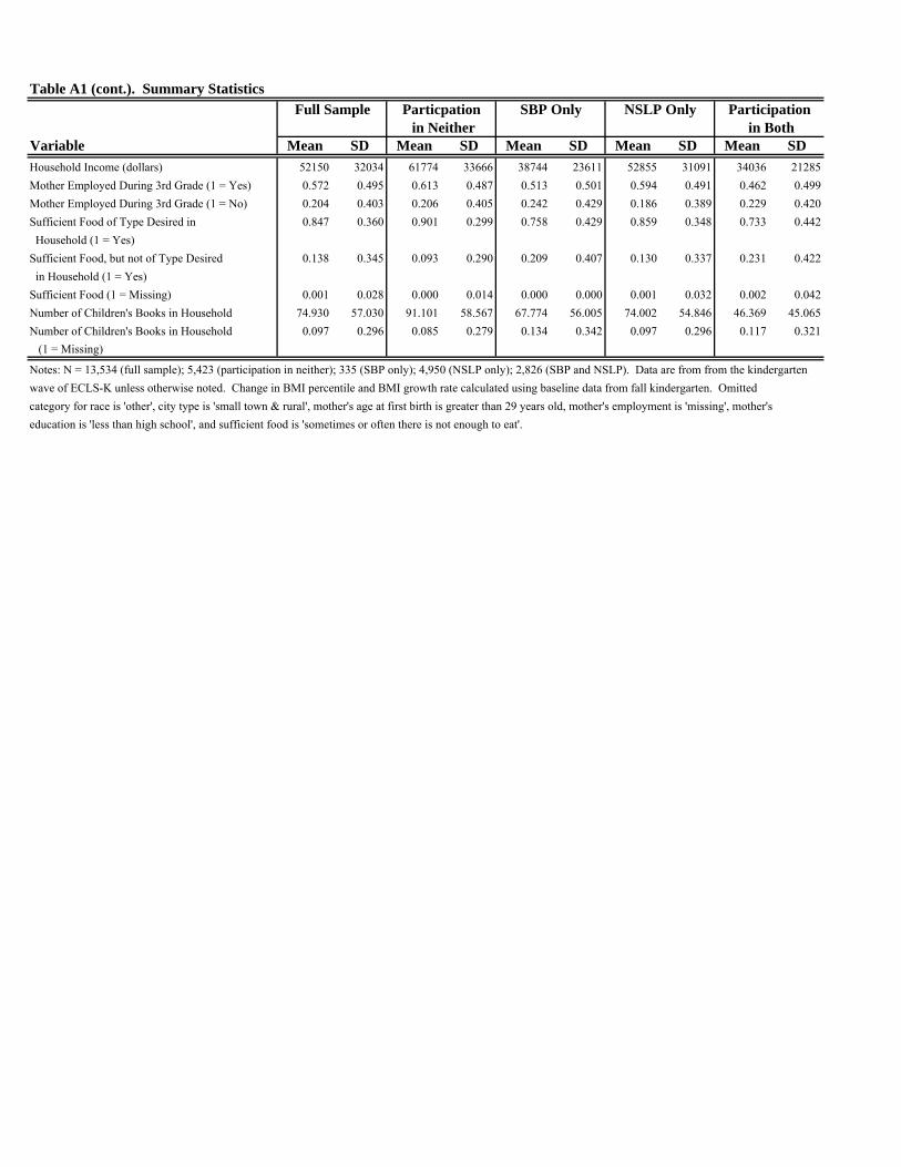
Table A1 (cont.). Summary Statistics
Variable Mean SD Mean SD Mean SD Mean SD Mean SDHousehold Income (dollars) 52150 32034 61774 33666 38744 23611 52855 31091 34036 21285Mother Employed During 3rd Grade (1 = Yes) 0.572 0.495 0.613 0.487 0.513 0.501 0.594 0.491 0.462 0.499Mother Employed During 3rd Grade (1 = No) 0.204 0.403 0.206 0.405 0.242 0.429 0.186 0.389 0.229 0.420Sufficient Food of Type Desired in 0.847 0.360 0.901 0.299 0.758 0.429 0.859 0.348 0.733 0.442 Household (1 = Yes)Sufficient Food, but not of Type Desired 0.138 0.345 0.093 0.290 0.209 0.407 0.130 0.337 0.231 0.422 in Household (1 = Yes)Sufficient Food (1 = Missing) 0.001 0.028 0.000 0.014 0.000 0.000 0.001 0.032 0.002 0.042Number of Children's Books in Household 74.930 57.030 91.101 58.567 67.774 56.005 74.002 54.846 46.369 45.065Number of Children's Books in Household 0.097 0.296 0.085 0.279 0.134 0.342 0.097 0.296 0.117 0.321 (1 = Missing)
Notes: N = 13,534 (full sample); 5,423 (participation in neither); 335 (SBP only); 4,950 (NSLP only); 2,826 (SBP and NSLP). Data are from from the kindergartenwave of ECLS-K unless otherwise noted. Change in BMI percentile and BMI growth rate calculated using baseline data from fall kindergarten. Omitted category for race is 'other', city type is 'small town & rural', mother's age at first birth is greater than 29 years old, mother's employment is 'missing', mother's education is 'less than high school', and sufficient food is 'sometimes or often there is not enough to eat'.
Participation in Neither in Both
Full Sample Particpation SBP Only NSLP Only

Table A2. Sensitivity Analysis: Bivariate Probit Results with Different Assumptions Concerning Correlation Among the Disturbances by Risk Type
ρ = 0 ρ = 0.1 ρ = 0.2 ρ = 0.3 ρ = 0.4 ρ = 0.5I. Normal Weight Entering Kindergarten
School 0.124* -0.043 -0.210* -0.377* -0.543* -0.709* Breakfast (0.042) (0.042) (0.042) (0.041) (0.040) (0.038) School -0.011 0.016 0.046 0.078† 0.112* 0.149* Lunch (0.035) (0.035) (0.035) (0.035) (0.034) (0.034)
School 0.155† -0.013 -0.180* -0.348* -0.516* -0.686* Breakfast (0.061) (0.060) (0.059) (0.058) (0.057) (0.055) School 0.008 0.037 0.070 0.107† 0.147* 0.192* Lunch (0.053) (0.053) (0.052) (0.052) (0.051) (0.050)
II. Obese or Overweight Entering Kindergarten
School -0.046 -0.213* -0.381* -0.548* -0.717* -0.887* Breakfast (0.065) (0.065) (0.065) (0.064) (0.063) (0.061) School -0.016 0.013 0.040 0.066 0.090 0.113† Lunch (0.057) (0.057) (0.057) (0.056) (0.056) (0.056)
School 0.032 -0.135† -0.301* -0.468* -0.633* -0.798* Breakfast (0.058) (0.058) (0.057) (0.057) (0.055) (0.053) School 0.027 0.056 0.086‡ 0.115† 0.145* 0.174* Lunch (0.050) (0.050) (0.050) (0.050) (0.050) (0.049)
NOTES: ‡ p<0.10, † p<0.05, * p<0.01. Standard errors in parentheses. Specification (1) refers to control set used in Column (1) in Table 1. See Tables 1, 4, and text for details.
Correlation of the Disturbances
B. Probability of Being Obese
A. Probability of Being Overweight
B. Probability of Being Obese
A. Probability of Being Overweight
Specification (1)

Table A3. Sensitivity Analysis: Amount of Selection on Unobservables Relative to Selection on Observables Required to Attribute the Entire SBP Effect to Selection Bias by Risk Type
Cov(ε,ν)÷ τ1 Implied Cov(ε,ν)÷ τ1 ImpliedVar(ν) Ratio Var(ν) Ratio
I. Normal Weight Entering Kindergarten BMI: Levels 8.825 0.305 0.035 1.002 0.243 0.242
(0.067) (0.059) BMI: Logs 0.437 0.017 0.038 0.051 0.013 0.261
(0.004) (0.003) BMI: Growth Rates 0.363 0.013 0.035 0.204 0.013 0.065
(0.003) (0.003) Percentile BMI: Levels 76.532 3.077 0.040 7.903 2.198 0.278
(0.798) (0.668) Percentile BMI: Changes 68.900 1.608 0.023 11.741 2.195 0.187
(0.716) (0.668) Probability of Being Overweight 4.561 0.033 0.007
(0.011) Probability of Being Obese 2.633 0.016 0.006
(0.006)
II. Obese or Overweight Entering Kindergarten BMI: Levels 14.461 0.272 0.019 0.837 0.177 0.211
(0.189) (0.131) BMI: Logs 0.561 0.010 0.017 0.037 0.006 0.170
(0.008) (0.006) BMI: Growth Rates 0.396 0.006 0.015 0.225 0.006 0.028
(0.006) (0.006) Percentile BMI: Levels 20.935 -0.081 -0.004 3.058 -0.179 -0.058
(0.620) (0.557) Percentile BMI: Changes 10.621 -0.147 -0.014 7.906 -0.179 -0.023
(0.559) (0.557) Probability of Being Overweight 0.640 -0.013 -0.021 0.640 -0.013 -0.021
(0.019) (0.019) Probability of Being Obese 2.531 0.012 0.005 0.395 0.007 0.017
(0.023) (0.020)
NOTES: Standard errors in parentheses. Specifications (1) and (2) refer to control sets used in Table 1. See Tables 1 and 5 for details.
Specification (1) Specification (2)

Table A4. Propensity Score Matching Sensitivity Analysis by Risk Type: Rosenbaum Bounds (SBP)Γ = 1 Γ = 1.2 Γ = 1.4 Γ = 1.6 Γ = 1.8 Γ = 2 Γ = 2.5 Γ = 3
I. Full Sample BMI: Levels p = 0.000 p = 0.000 p = 0.411 p = 1.000 p = 1.000 p = 1.000 p = 1.000 p = 1.000 BMI: Logs p = 0.000 p = 0.000 p = 0.996 p = 1.000 p = 1.000 p = 1.000 p = 1.000 p = 1.000 BMI: Growth Rates p = 0.000 p = 0.000 p = 0.873 p = 1.000 p = 1.000 p = 1.000 p = 1.000 p = 1.000 Percentile BMI: Levels p = 0.000 p = 0.989 p = 1.000 p = 1.000 p = 1.000 p = 1.000 p = 1.000 p = 1.000 Percentile BMI: Changes p = 0.000 p = 0.000 p = 0.718 p = 1.000 p = 1.000 p = 1.000 p = 1.000 p = 1.000 Prob. of Being Overweight p = 0.071 p = 1.000 p = 1.000 p = 1.000 p = 1.000 p = 1.000 p = 1.000 p = 1.000 Prob. of Being Obese p = 0.000 p = 0.000 p = 0.000 p = 0.000 p = 0.828 p = 1.000 p = 1.000 p = 1.000
II. Normal Weight Entering Kindergarten BMI: Levels p = 0.000 p = 0.000 p = 0.069 p = 1.000 p = 1.000 p = 1.000 p = 1.000 p = 1.000 BMI: Logs p = 0.000 p = 0.000 p = 0.840 p = 1.000 p = 1.000 p = 1.000 p = 1.000 p = 1.000 BMI: Growth Rates p = 0.000 p = 0.000 p = 0.000 p = 0.985 p = 1.000 p = 1.000 p = 1.000 p = 1.000 Percentile BMI: Levels p = 0.000 p = 0.487 p = 1.000 p = 1.000 p = 1.000 p = 1.000 p = 1.000 p = 1.000 Percentile BMI: Changes p = 0.000 p = 0.000 p = 0.610 p = 1.000 p = 1.000 p = 1.000 p = 1.000 p = 1.000 Prob. of Being Overweight p = 0.000 p = 0.000 p = 0.000 p = 0.000 p = 0.000 p = 0.064 p = 1.000 p = 1.000 Prob. of Being Obese p = 0.000 p = 0.000 p = 0.000 p = 0.000 p = 0.000 p = 0.000 p = 0.000 p = 0.000
III. Obese or Overweight Entering Kindergarten BMI: Levels p = 0.000 p = 0.000 p = 0.491 p = 1.000 p = 1.000 p = 1.000 p = 1.000 p = 1.000 BMI: Logs p = 0.000 p = 0.002 p = 0.826 p = 1.000 p = 1.000 p = 1.000 p = 1.000 p = 1.000 BMI: Growth Rates p = 0.000 p = 0.335 p = 1.000 p = 1.000 p = 1.000 p = 1.000 p = 1.000 p = 1.000 Percentile BMI: Levels p = 0.966 p = 1.000 p = 1.000 p = 1.000 p = 1.000 p = 1.000 p = 1.000 p = 1.000 Percentile BMI: Changes p = 1.000 p = 1.000 p = 1.000 p = 1.000 p = 1.000 p = 1.000 p = 1.000 p = 1.000 Prob. of Being Overweight p = 0.527 p = 1.000 p = 1.000 p = 1.000 p = 1.000 p = 1.000 p = 1.000 p = 1.000 Prob. of Being Obese p = 0.000 p = 0.000 p = 0.000 p = 0.000 p = 0.000 p = 0.191 p = 1.000 p = 1.000
NOTES: Rosenbaum critical p-values for test of the null of zero average treatment effect. For controls included in the propensty score, see Table 1.

Figure 1. Theoretical Impact of Infra-Marginal Food Transfer Programs on Food and Non-Food Consumption. NOTES: A – initial consumption point prior to food transfer program. B – final consumption point with food transfer program assuming food and non-food consumption are normal goods. C – final consumption point with food transfer program assuming non-food consumption is a normal good and the income elasticity of food consumption is zero.
Non-food consumption
B
A
C
food
I0I1
I1’
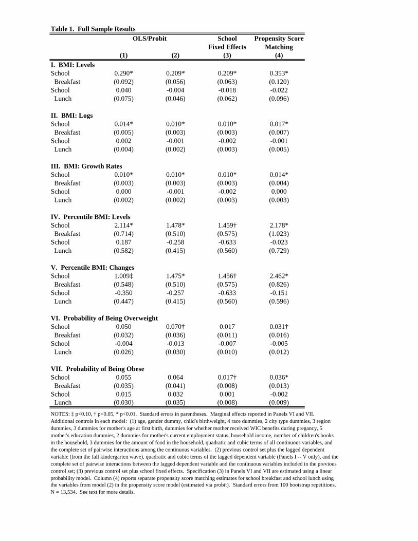
Table 1. Full Sample ResultsSchool Propensity Score
Fixed Effects Matching(1) (2) (3) (4)
I. BMI: LevelsSchool 0.290* 0.209* 0.209* 0.353* Breakfast (0.092) (0.056) (0.063) (0.120)School 0.040 -0.004 -0.018 -0.022 Lunch (0.075) (0.046) (0.062) (0.096)
II. BMI: LogsSchool 0.014* 0.010* 0.010* 0.017* Breakfast (0.005) (0.003) (0.003) (0.007)School 0.002 -0.001 -0.002 -0.001 Lunch (0.004) (0.002) (0.003) (0.005)
III. BMI: Growth RatesSchool 0.010* 0.010* 0.010* 0.014* Breakfast (0.003) (0.003) (0.003) (0.004)School 0.000 -0.001 -0.002 0.000 Lunch (0.002) (0.002) (0.003) (0.003)
IV. Percentile BMI: LevelsSchool 2.114* 1.478* 1.459† 2.178* Breakfast (0.714) (0.510) (0.575) (1.023)School 0.187 -0.258 -0.633 -0.023 Lunch (0.582) (0.415) (0.560) (0.729)
V. Percentile BMI: ChangesSchool 1.009‡ 1.475* 1.456† 2.462* Breakfast (0.548) (0.510) (0.575) (0.826)School -0.350 -0.257 -0.633 -0.151 Lunch (0.447) (0.415) (0.560) (0.596)
VI. Probability of Being OverweightSchool 0.050 0.070† 0.017 0.031† Breakfast (0.032) (0.036) (0.011) (0.016)School -0.004 -0.013 -0.007 -0.005 Lunch (0.026) (0.030) (0.010) (0.012)
VII. Probability of Being ObeseSchool 0.055 0.064 0.017† 0.036* Breakfast (0.035) (0.041) (0.008) (0.013)School 0.015 0.032 0.001 -0.002 Lunch (0.030) (0.035) (0.008) (0.009)
the variables from model (2) in the propensity score model (estimated via probit). Standard errors from 100 bootstrap repetitions. N = 13,534. See text for more details.
NOTES: ‡ p<0.10, † p<0.05, * p<0.01. Standard errors in parentheses. Marginal effects reported in Panels VI and VII. Additional controls in each model: (1) age, gender dummy, child's birthweight, 4 race dummies, 2 city type dummies, 3 region dummies, 3 dummies for mother's age at first birth, dummies for whether mother received WIC benefits during pregancy, 5 mother's education dummies, 2 dummies for mother's current employment status, household income, number of children's books in the household, 3 dummies for the amount of food in the household, quadratic and cubic terms of all continuous variables, and the complete set of pairwise interactions among the continuous variables. (2) previous control set plus the lagged dependent variable (from the fall kindergarten wave), quadratic and cubic terms of the lagged dependent variable (Panels I -- V only), and the complete set of pairwise interactions between the lagged dependent variable and the continuous variables included in the previous control set; (3) previous control set plus school fixed effects. Specification (3) in Panels VI and VII are estimated using a linear probability model. Column (4) reports separate propensity score matching estimates for school breakfast and school lunch using
OLS/Probit

Table 2. Results: Children by Risk Type Entering Kindergarten
OLS/Probit School Propensity OLS/Probit School PropensityFixed Score Fixed Score
Effects Matching Effects Matching(1) (2) (3) (1) (2) (3)
I. BMI: Growth RatesSchool 0.013* 0.014* 0.017* 0.006 0.001 0.012‡ Breakfast (0.003) (0.004) (0.005) (0.006) (0.007) (0.007)School 0.000 -0.004 0.001 0.000 0.000 -0.002 Lunch (0.003) (0.004) (0.003) (0.005) (0.008) (0.006)
II. Percentile BMI: ChangesSchool 1.608† 2.096* 3.211* -0.147 -0.482 0.227 Breakfast (0.716) (0.761) (0.987) (0.559) (0.708) (0.655)School -0.303 -0.800 0.042 -0.397 -0.589 -0.534 Lunch (0.571) (0.719) (0.594) (0.485) (0.750) (0.555)
III. Probability of Being OverweightSchool 0.124* 0.033* 0.032† -0.046 -0.016 0.016 Breakfast (0.042) (0.012) (0.015) (0.065) (0.024) (0.021)School -0.011 -0.010 0.000 -0.016 -0.004 -0.012 Lunch (0.035) (0.012) (0.010) (0.057) (0.025) (0.018)
IV. Probability of Being ObeseSchool 0.155† 0.022* 0.021† 0.032 0.011 0.101* Breakfast (0.061) (0.007) (0.009) (0.058) (0.025) (0.026)School 0.008 -0.004 0.001 0.027 0.003 -0.019 Lunch (0.053) (0.006) (0.005) (0.050) (0.027) (0.022)NOTES: ‡ p<0.10, † p<0.05, * p<0.01. Standard errors in parentheses. N = 10,039 (Normal) and 3,495 (Overweight or Obese). Specification (1) is identical to Specification (1) in Table 1; Specifications (2) and (3) are analagous to Specifications (3) and (4) in Table 1. Specification (2) in Panels III and IV is estimated using a linear probability model; in addition, these models exclude lagged values of the dependent variable in Model A since there is no variation by construction. See Table 1 for additional details.
Entering KindergartenNormal Weight Range Overweight or Obese

Table 3. Selection into School Nutrition Programs
OLS School Propensity OLS School Propensity OLS School PropensityFixed Score Fixed Score Fixed Score
Effects Matching Effects Matching Effects Matching(1) (2) (3) (1) (2) (3) (1) (2) (3)
I. Weight (lbs.)School 0.038 0.053 0.371 0.069 0.065 -0.101 -0.089 0.098 1.034‡ Breakfast (0.154) (0.175) (0.313) (0.091) (0.104) (0.171) (0.328) (0.411) (0.620)School 0.134 0.147 0.003 0.056 0.014 0.108 0.242 -0.081 -0.298 Lunch (0.125) (0.170) (0.210) (0.073) (0.098) (0.137) (0.284) (0.437) (0.526)N
II. Weight (lbs.): Change in LevelsSchool 0.067 0.084 0.402 0.098 0.096 -0.055 -0.074 0.103 1.166‡ Breakfast (0.154) (0.175) (0.274) (0.091) (0.104) (0.177) (0.328) (0.412) (0.651)School 0.137 0.151 0.011 0.058 0.022 0.110 0.196 -0.097 -0.339 Lunch (0.125) (0.171) (0.180) (0.073) (0.099) (0.105) (0.284) (0.437) (0.486)N
III. Weight (lbs.): LogsSchool 0.001 0.001 0.007 0.002 0.002 -0.002 -0.002 0.000 0.016 Breakfast (0.003) (0.003) (0.006) (0.002) (0.002) (0.004) (0.005) (0.007) (0.012)School 0.003 0.003 0.001 0.001 0.000 0.003 0.004 0.000 -0.004 Lunch (0.002) (0.003) (0.004) (0.002) (0.002) (0.003) (0.005) (0.007) (0.008)N
IV. Weight (lbs.): Growth RatesSchool 0.011* 0.012* 0.021* 0.013* 0.014* 0.014 0.004 0.007 0.030‡ Breakfast (0.004) (0.004) (0.009) (0.004) (0.004) (0.009) (0.007) (0.008) (0.016)School 0.002 0.003 0.003 0.001 0.002 0.003 0.003 -0.001 -0.006 Lunch (0.003) (0.004) (0.005) (0.003) (0.004) (0.006) (0.006) (0.009) (0.011)N
NOTES: ‡ p<0.10, † p<0.05, * p<0.01. Standard errors in parentheses. Specification (1) is identical to Specification (1) in Table 1, except all terms involving child's birthweight are omitted in Panels II and IV; Specifications (2) and (3) are similarly analagous to Specifications (3) and (4) in Table 1. In addition, all regressions include controls for child's height in fall kindergarten (plus higher order and interaction terms). See Table 1 and text for details.
Entering Kindergarten Entering Kindergarten
Full Sample Risk TypeNormal Weight Overweight or Obese
13534
13534 10039 3495
10039 3495
13534
13534 10039 3495
10039 3495

Table 4. Sensitivity Analysis: Bivariate Probit Results with Different Assumptions Concerning Correlation Among the Disturbances
ρ = 0 ρ = 0.1 ρ = 0.2 ρ = 0.3 ρ = 0.4 ρ = 0.5 ρ = 0 ρ = 0.1 ρ = 0.2 ρ = 0.3 ρ = 0.4 ρ = 0.5
School 0.050 -0.117* -0.284* -0.449* -0.614* -0.778* 0.070† -0.097* -0.264* -0.431* -0.598* -0.766* Breakfast (0.032) (0.031) (0.031) (0.031) (0.030) (0.029) (0.036) (0.035) (0.035) (0.034) (0.034) (0.033) School -0.004 0.023 0.052† 0.082* 0.113* 0.145* -0.013 0.015 0.044 0.074† 0.106* 0.139* Lunch (0.026) (0.026) (0.026) (0.026) (0.026) (0.026) (0.030) (0.030) (0.029) (0.029) (0.029) (0.029)
School 0.055 -0.112* -0.278* -0.444* -0.608* -0.771* 0.064 -0.103† -0.270* -0.436* -0.603* -0.770* Breakfast (0.035) (0.035) (0.035) (0.034) (0.033) (0.032) (0.041) (0.041) (0.040) (0.040) (0.039) (0.038) School 0.015 0.044 0.075† 0.108* 0.144* 0.182* 0.032 0.061‡ 0.092* 0.125* 0.160* 0.199* Lunch (0.030) (0.030) (0.030) (0.030) (0.029) (0.029) (0.035) (0.035) (0.035) (0.034) (0.034) (0.033)
NOTES: ‡ p<0.10, † p<0.05, * p<0.01. Standard errors in parentheses. Specifications (1) and (2) refer to control sets used in Table 1. See Table 1 and text for details.
B. Probability of Being Obese
Correlation of the DisturbancesSpecification (1) Specification (2)
A. Probability of Being Overweight

Table 5. Sensitivity Analysis: Amount of Selection on Unobservables Relative to Selection on Observables Required to Attribute the Entire SBP Effect to Selection Bias
Cov(ε,ν)÷ τ1 Implied Cov(ε,ν)÷ τ1 ImpliedVar(ν) Ratio Var(ν) Ratio
BMI: Levels 14.625 0.290 0.020 0.453 0.209 0.460(0.092) (0.056)
BMI: Logs 0.654 0.014 0.022 0.024 0.010 0.405(0.005) (0.003)
BMI: Growth Rates 0.490 0.010 0.021 0.175 0.010 0.057(0.003) (0.003)
Percentile BMI: Levels 77.583 2.114 0.027 4.465 1.478 0.331(0.714) (0.510)
Percentile BMI: Changes 57.727 1.009 0.017 7.718 1.475 0.191(0.548) (0.510)
Probability of Being Overweight 3.313 0.019 0.006 0.327 0.019 0.058(0.011) (0.009)
Probability of Being Obese 3.450 0.015 0.004 0.456 0.012 0.027(0.009) (0.007)
NOTES: Standard errors in parentheses. Specifications (1) and (2) refer to control sets used in Table 1, plus NSLP participation. Cov(ε,ν)/Var(ν) refers to the asymptotic bias of the unconstrained estimate under the assumption of equal (normalized) selection on observables and unobservables. τ1 refers to the unconstrained estimate of the
effect of SBP participation. The implied ratio is the latter divided by the former. See Table 1 and text for details.
Specification (1) Specification (2)