Scalar flux profile relationships over the open ocean

J. B. Edson, C. J. Zappa,1 J. A. Ware, and W. R. McGillis2

Woods Hole Oceanographic Institution, Woods Hole, Massachusetts, USA

J. E. Hare3

Environmental Technologies Laboratory, National Oceanic and Atmospheric Administration, Boulder, Colorado, USA

Received 15 May 2003; revised 5 March 2004; accepted 14 May 2004; published 14 August 2004.

[1] The most commonly used flux-profile relationships are based on Monin-Obukhov(MO) similarity theory. These flux-profile relationships are required in indirect methodssuch as the bulk aerodynamic, profile, and inertial dissipation methods to estimate thefluxes over the ocean. These relationships are almost exclusively derived from previousfield experiments conducted over land. However, the use of overland measurements toinfer surface fluxes over the ocean remains questionable, particularly close to the oceansurface where wave-induced forcing can affect the flow. This study investigates the fluxprofile relationships over the open ocean using measurements made during the 2000Fluxes, Air-Sea Interaction, and Remote Sensing (FAIRS) and 2001 GasEx experiments.These experiments provide direct measurement of the atmospheric fluxes along withprofiles of water vapor and temperature. The specific humidity data are used to determineparameterizations of the dimensionless gradients using functional forms of two commonlyused relationships. The best fit to the Businger-Dyer relationship [Businger, 1988] isfound using an empirical constant of aq = 13.4 ± 1.7. The best fit to a formulation that hasthe correct form in the limit of local free convection [e.g., Wyngaard, 1973] is found usingaq = 29.8 ± 4.6. These values are in good agreement with the consensus values fromprevious overland experiments and the Coupled Ocean-Atmosphere Response Experiment(COARE) 3.0 bulk algorithm [Fairall et al., 2003]; e.g., the COARE algorithm usesempirical constants of 15 and 34.2 for the Businger-Dyer and convective forms,respectively. Although the flux measurements were made at a single elevation and localsimilarity scaling is applied, the good agreement implies that MO similarity is validwithin the marine atmospheric surface layer above the wave boundary layer. INDEX

TERMS: 0312 Atmospheric Composition and Structure: Air/sea constituent fluxes (3339, 4504); 1655 Global

Change: Water cycles (1836); 3307 Meteorology and Atmospheric Dynamics: Boundary layer processes; 4247

Oceanography: General: Marine meteorology; KEYWORDS: air-sea fluxes, flux profile relationships, marine

boundary layer

Citation: Edson, J. B., C. J. Zappa, J. A. Ware, W. R. McGillis, and J. E. Hare (2004), Scalar flux profile relationships over the open

ocean, J. Geophys. Res., 109, C08S09, doi:10.1029/2003JC001960.

1. Introduction

[2] Over the ocean, direct measurement of turbulentfluxes is often complicated by platform motion, flowdistortion, and the effects of sea spray. Because of this,marine meteorologists and oceanographers have long reliedon flux profile relationships that relate the turbulence fluxesof momentum, heat, and moisture (or mass) to their respec-tive profiles of velocity, temperature, and water vapor (or

other gases). These flux profile relationships are required inindirect methods such as the bulk aerodynamic, profile, andinertial dissipation methods that estimate the fluxes frommean, profile, and high-frequency spectral measurements,respectively. The flux profile or gradient flux relationshipsare also used extensively in numerical models to providelower boundary conditions and to ‘‘close’’ the model byapproximating higher-order terms from low-order variables.The most commonly used flux-profile relationships arebased on Monin-Obukhov (MO) similarity theory. MOsimilarity theory predicts that the nondimensional gradientof velocity, temperature, and humidity are universal func-tions of atmospheric stability

kzx*

@X

@z¼ fx

z

L

� �ð1Þ

JOURNAL OF GEOPHYSICAL RESEARCH, VOL. 109, C08S09, doi:10.1029/2003JC001960, 2004

1Now at Ocean and Climate Physics Division, Lamont-Doherty EarthObservatory, Columbia University, Palisades, New York, USA.

2Now at Geochemistry Division, Lamont-Doherty Earth Observatory,Columbia University, Palisades, New York, USA.

3Also at Cooperative Institute for Research in Environmental Sciences,University of Colorado, Boulder, Colorado, USA.

Copyright 2004 by the American Geophysical Union.0148-0227/04/2003JC001960$09.00

C08S09 1 of 15

where x = u, q, q denotes velocity, potential temperature,and specific humidity, respectively; x* is the scalingparameter for the variable x; k is von Karman’s constantz; is the height above the surface; X represents the meanof the variable x; and z/L is a stability parameter where Lis the MO length. The stability parameter �z/L representsthe ratio of buoyant production (convection) to mechan-ical production (shear) in a constant flux layer. As such,it is closely related to the flux Richardson number, whichis more commonly used in investigation of the oceanicmixed layer.[3] These flux-profile relationships have been investigated

during overland experiments including the tower studies byDyer and Hicks [1970] and Carl et al. [1973], the land-mark Kansas and International Turbulence Comparision(ITCE) experiments [e.g., Businger et al., 1971; Dyerand Bradley, 1982], and more recently in the experimentdescribed by Hogstrom [1988], Frenzen and Vogel [1992,2001], Oncley et al. [1996], and Poulos et al. [2002]. Theseand other experiments have generated a number of similarsemiempirical functions, with the most commonly usedforms known as the Businger-Dyer formulae [Businger,1988].[4] While the majority of the investigations were con-

ducted over land, several notable exceptions have beenconducted over water. Badgley and Paulson [1972] andPaulson et al. [1972a] describe measurements of wind,temperature, and humidity profiles over the Arabian Seaduring the 1964 International Indian Ocean Expedition.They report results that are consistent with Businger-Dyerformulae. However, they did not directly measure thefluxes, so they could not directly investigate the flux-profilerelationships. Miyake et al. [1970] measured turbulentfluxes and profiles from two masts located in a fetch limitedlocation over the sea. They found the profile and directcovariance estimates to agree well within the experimentalerror using Businger-Dyer formulae. However, they did notattempt to refine the flux-profile relationships, presumablybecause of the limited range of stability. Pond et al. [1971]and Paulson et al. [1972b] measured velocity, temperature,and humidity profiles and their associated fluxes duringBarbados Oceanographic and Meteorological Experiment(BOMEX) aboard the R/P FLIP. However, uncertainty intheir velocity profiles caused by flow distortion aroundFLIP as well as salt contamination of the temperatureprofiles and flux estimates also limited their analyses tocomparisons of profile and direct covariance flux estimatesusing Businger-Dyer formulae.[5] As a result, the semiempirical formulae developed

over land remain widely used in indirect methods such asthe bulk aerodynamic and inertial dissipation methods toestimate the turbulent fluxes over the ocean. However, theuse of overland measurements to infer surface fluxes overthe ocean remains questionable, particularly close to theocean surface where wave-induced forcing can affect theflow. For example, recent investigations of the dimension-less shear over the ocean byMiller et al. [1997], Vickers andMahrt [1999], and Smedman et al. [1999] report wave-induced effects that can cause substantial departure fromMO similarity predictions. Therefore the universality ofthese relationships to all surface layers is a current topicof intense debate.

[6] This paper investigates scalar flux profiles over theopen ocean using data from two field experiments. Theatmospheric stability during these experiments was predom-inantly unstable and the analysis is limited to an investiga-tion of the dimensionless profile functions under theseconditions. A brief description of the underlying principlesused in MO similarity theory followed by a more detaileddiscussion of the semiempirical functions is provided insection 2. The experimental setups used during these twoexperiments are described in section 3. Section 4 presentsthe results from the experiments and compares them withprevious investigations over land and water.

2. Monin-Obukhov Similarity Theory

[7] Monin-Obukhov similarity theory provides a power-ful statistical tool for studies of atmospheric turbulence inthe surface layer. At its foundation is the assumption thatflows with similar ratios of convective to mechanicalgeneration of turbulence at a given height (i.e., similarRichardson numbers) are expected to have similar turbulentstructures. Specifically, MO similarity theory states that thestructure of turbulence in a constant flux layer is determinedby the height above the surface, z; the buoyancy parameter,g/Qv, where is gravity and Qv is the mean virtual potentialtemperature; the friction velocity, u*, and the surface buoy-ancy flux, wqvs, where and qv are the fluctuating verticalvelocity and virtual potential temperature, respectively, andthe subscript denotes the surface value. The friction velocityis derived from the surface stress

u*¼ ts

ra

� �1=2¼ Fu 0ð Þj j1=2 ð2Þ

while the buoyancy flux can be broken down as

wqvs ¼Qh

racpþ 0:61Ts

Qe

raLe¼ Fq 0ð Þ þ 0:61TsFq 0ð Þ ð3Þ

where ts is the surface stress vector, Qh is the surface valueof the sensible heat flux, Qe is the surface value of the latentheat flux, Ts is the surface temperature, cp is the specific heatat constant pressure, Le is the latent heat of vaporization ofwater, and, Fu, Fq and Fq are the kinematic forms [e.g., seeStull, 1988] of the momentum, sensible heat, and latent heatfluxes, respectively. These quantities define the additionalscaling parameters as

x*� �Fx 0ð Þ

u*

ð4Þ

as well as the MO length

L ¼ �Qv

gk

u3*

wqvs¼ Qv

gk

u2*

q*þ 0:61Tsq*

� � ð5Þ

The similarity hypothesis then states that various turbulentstatistics, when normalized by these scaling parameters, areuniversal functions of z/L.

C08S09 EDSON ET AL.: OCEANIC SCALAR FLUX-PROFILE RELATIONSHIPS

2 of 15

C08S09

[8] These functions are commonly used to provide indi-rect estimates of the surface fluxes over the ocean. Forexample, equations (1) and (4) can be combined to provideparameterizations for the fluxes given by

Fx ¼ �u*kz

fx zð Þ@X

@z¼ Kx

@X

@zð6Þ

where, z = z/L, and Kx are the eddy diffusivities as definedusing MO similarity. This parameterization is the basis forthe gradient flux method. Note that the eddy diffusivities formomentum and heat, denoted by Ku and Kq, are morecommonly denoted by Km and Kh. The notation used inequation (6) avoids mixing subscripts and is thereforeemployed for simplicity.[9] These scaling laws are expected to hold and the

derived parameterizations are expected to be universal aslong as the assumptions that govern the MO similarity lawsare valid, i.e., a combination of mechanical and thermalforcing drive the turbulent exchange, the scaling variablesare independent of height in the surface layer, and theturbulence statistics are stationary and horizontally homo-geneous. The constant flux layer constraint is generallyassumed to be valid in the lowest 10% of the unstableatmospheric boundary layer.[10] In highly stratified boundary layers where large flux

divergences are observed even close to the surface, theconstant flux assumption is often relaxed resulting in anextension of MO similarity known as local similarity theory[cf. Mahrt, 1998]. Local similarity uses the local value ofthe fluxes to define scaling parameters that may vary withheight. An accurate implementation of this approachrequires normalization of the gradients using local valuesof the gradient and scaling parameters. This is also the mostaccurate application of MO similarity theory when only onelevel of flux estimates is available, i.e., the local unadjustedvalues of the fluxes are used to scale the local gradientscomputed at the level of the flux estimates. This describesthe experimental setup used in the investigations, i.e., thefluxes are computed at a single elevation. Therefore thispaper uses the local similarity approach to investigatefunctional forms of the dimensionless water vapor profilesgiven by equation (1).[11] Finally, these assumptions can also become invalid in

the lowest 10% of the marine boundary layer when waveinduced flow plays an important role in turbulent exchange.This near surface region of the marine boundary layer isreferred to as the wave boundary layer (WBL). At present,there is no consensus definition for the height of the WBL.For example, many numerical modelers assume that theinfluence of the waves is limited to the region wherez/sH � 1, where sH is the significant wave height of thedominant waves [e.g., Janssen, 1989; Makin et al., 1995].However, recent field campaigns have shown that someturbulent statistics, e.g., the pressure transport term in thekinetic energy budget equation [Hare et al., 1997; Edsonand Fairall, 1998; Hristov et al., 2003], are influenced bywaves up to heights where kpz 2, where is the peak wavenumber of the dominant waves. The latter findings suggest asubstantially thicker WBL for some characteristics of theflow.

[12] Most investigations assume that the transfer of heatand mass is less affected by ocean waves than the transfer ofmomentum and kinetic energy. The physical argumentbehind this assumption is that the momentum flux can becarried by both tangential stress and the normal stress, orform drag, created by interaction between the pressure andwave fields. The form drag and energy input to the wavesappear as source/sink term in the momentum and kineticenergy budgets, respectively [e.g., Edson and Fairall, 1998;Janssen, 1999]. However, the equivalent of a normal stressdoes not exist in the heat or scalar variance budgets due tothe absence of pressure terms. This translates to the absenceof a wave-induced heat or mass flux over waves [Makin etal., 1995].[13] This does not mean that the effect of waves on

heat and mass transfer is necessarily negligible since theeddy diffusivities in equation (6) are expected to bemodulated by waves [e.g., Makin and Mastenbroek,1996]. As a result, the turbulent flux of heat and massis also expected to be modulated by waves. Additionally,the presence of evaporating sea-spray is expected toinfluence the transfer of heat and mass at high winds[e.g., Fairall et al., 1994; Makin, 1998; Andreas andEmanuel, 2001]. However, there is considerable debateabout the type of conditions required to observe asignificant impact on the fluxes.

2.1. Functional Forms for Unstable AtmosphericBoundary Layers

[14] Forty years of experimental dimensionless profileinvestigations have lead to a myriad of parameterizationsand even more investigations to address the universality ofthese functions. However, it has become common practiceto parameterize the dimensionless profiles in unstable con-ditions using

fx zð Þ ¼ gx 1� axzð Þ�Nx ð7Þ

where ax and Nx are numerical constants and gx is the valueof the dimensionless profile under neutral conditions. Thevalues of the dimensionless temperature and humidityprofiles under neutral conditions are closely related to theturbulent Prandtl and Schmidt numbers, respectively. Forexample, the turbulent Schmidt number, Sc, is defined as theratio of the eddy diffusivity for momentum, Ku, over theeddy diffusivity for mass, Kq. MO similarity predicts thatthe ratio of the eddy diffusivities is related to thedimensionless functions as

Sc ¼ Ku

Kq

¼fq zð Þfu zð Þ ð8Þ

Therefore the neutral values of the dimensionless functionare related by

gx

gu¼ Ku z ¼ 0ð Þ

Kx z ¼ 0ð Þ ¼fx 0ð Þfu 0ð Þ ð9Þ

such that by definition the neutral value of the dimension-less shear, gu, is equal to 1. This condition sets the value ofthe von Karman’s constant k. This relationship also equates

C08S09 EDSON ET AL.: OCEANIC SCALAR FLUX-PROFILE RELATIONSHIPS

3 of 15

C08S09

the neutral value of the turbulent Schmidt number, Sc0, withthe neutral value of the dimensionless humidity profile, gq.[15] There is considerable consensus in the meteorolog-

ical community on the value of the exponential constantin equation (7). In unstable conditions over the range �2 <z/L < 0, a number of field experiments [e.g., Dyer andHicks, 1970; Businger et al., 1971; Dyer and Bradley, 1982]have lead to the empirical relationships

Ku

Ky

¼ gyfu zð Þ ð10Þ

and

fu zð Þ ¼ 1� auzð Þ1=4 ð11Þ

where y = q, q and au is the numerical constant for thevelocity profile. The combination of equations (8), (10), and(11) results in a value of 1/2 for Ny in the parameterizationof both fq and fq. The scalar parameterizations using Ny =1/2 have also been shown to give good agreement withpotential temperature observations over the stability range�2 < z/L < 0 by these investigators. This set of functions,i.e., with Nu = 1/4 and Ny = 1/2, are known as Businger-Dyer formulae [Businger, 1988].[16] The dimensionless profiles for all variables are

expected to become proportional to (�z)1/3 in the limit offree convection [Gurvich, 1965;Wyngaard, 1973]. Thereforeseveral formulae withNx = 1/3 have been proposed [e.g.,Carlet al., 1973; Frenzen and Vogel, 2001]. While these formulaeoften give good agreement with data in very unstable con-ditions, they are inferior to the Businger-Dyer formulae nearneutral conditions. The KEYPS equation [e.g., Panofsky etal., 1960] provided a formula that incorporated the observednear neutral conditions with the expected behavior in con-vective limit. However, this equation is difficult to use inpractice to estimate the fluxes from indirect methods. A lesselegant but more easily implemented approach is used in theTropical Ocean-Global Atmosphere (TOGA)-CoupledOcean-Atmosphere Response Experiment (COARE) bulkalgorithm [Fairall et al., 1996]. The algorithm smoothlyblends the Businger-Dyer and convective forms to provide aparameterization with the expected behavior in both near-neutral and convective conditions [Grachev et al., 2000].[17] On the other hand, there remains considerable dis-

agreement on the values for k, gy, au and ay as shown inTable 1. Recent studies by Oncley et al. [1996], Frenzen andVogel [2001], and Andreas et al. [2002] have suggested thatthe von Karman’s constant is actually a variable that depends

on the roughness Reynolds number, Reo = zou*/n, where zo isthe roughness length and is the kinematic viscosity. If true,one would expect to find different values of the numericalconstants at different sites due to the inclusion of the vonKarman’s constant in the definition of L [cf. Yaglom, 1977].Yaglom [1977] and Hogstrom [1988] developed approachestomodify functions from different experiments such that theyused the same values for k and gy. As shown in Table 1,Hogstrom’s [1988] approach reduces the differences betweenthe various formulae after adjustments to the coefficients thatassume gy = 1 and k = 0.4. The inclusion of several fieldprograms since his study provide consensus values of 13.2and 20.5 for ay and au, respectively.

3. Experiment Setup

[18] Direct measurements of the atmospheric fluxes alongwith profiles of water vapor and temperature were madeduring the 2000 Fluxes, Air-Sea Interaction, and RemoteSensing (FAIRS) and 2001 GasEx experiments. The FAIRSexperiment took place from 15 September to 15 October2000 aboard the R/P FLIP. The data used in the presentanalysis were taken during the first leg of the cruise from 23to 30 September (yeardays 267 to 274). The FLIP wasallowed to drift during this experiment and was located about200 km west of the central California coast centered around34N, 124W. The GasEx-01 experiment took place in theequatorial Pacific aboard the National Oceanic and Atmo-spheric Administration (NOAA) R/V Ronald H. Brown. Thedata used in this investigation was collected from 14 to28 February 2001 (yeardays 45 to 60). The R/V Brownoperated just south of the equator at 3S between thelongitudes 122W to 150W.

3.1. Direct Covariance Fluxes

[19] A flux package was deployed during the FAIRSexperiment on a mast that placed the sensors 3 m abovethe port boom as shown in Figure 1. The mast was locatedroughly 15 m from FLIP’s superstructure and 13.3 m abovethe ocean surface. The package included a three-axis sonicanemometer/thermometer (Solent R2), an open path infra-red hygrometer/CO2 sensor (Licor 7500), a three-axisaccelerometer/angular rate sensor (Systron Donner Motion-Pak), magnetic compass (Precision Navigation), and arelative humidity/temperature sensor (Vaisala HMP45).The velocity measurements were motion-corrected usingthe approach given by Edson et al. [1998]. Turbulentfluxes of momentum, heat, and moisture were computedover 15-min intervals. Time series of the turbulent fluxesused in this investigation are shown in Figure 2.

Table 1. Numerical Constants for the Businger-Dyer Formulae From Previous Field Experiments

Investigation

Experimental

AdjustedAccording toYaglom [1977]

AdjustedAccording to

Hogstrom [1988]

k gy au ay au ay au ay

Dyer and Hicks [1970] 0.41 1.0 16 16 16.4 16.4 16 16Businger et al. [1971] 0.35 0.74 15 9 13.1 7.9 20.3 12.2Dyer and Bradley [1982] 0.40 1.0 28 14 28 14 28 14Oncley et al. [1996] 0.37 0.86 15 9 13.7 8.2 17.4 10.5Frenzen and Vogel [2001] 0.38 - 21 - 20.1 - 21 -Average of Values 0.38 0.9 21 12 18.3 11.6 20.5 13.2

C08S09 EDSON ET AL.: OCEANIC SCALAR FLUX-PROFILE RELATIONSHIPS

4 of 15

C08S09

[20] During the GasEx-01 experiment, turbulent fluxmeasurements were made from the end of a boom thatplaced the sensors 10 m upwind of the bow as shown inFigure 3. Turbulent fluxes of momentum, heat, and watervapor were made by two flux packages: one was identical tothe FAIR’s package, while the other used a Solent R3anemometer and Crossbow DMU motion-sensing package.Time series of the fluxes from these packages are shown inFigure 4. The fluxes from the Solent R2 package were usedfor relative wind directions to starboard of bow-on flow,while the fluxes from the Solent R3 package were used forrelative wind directions to port of bow-on flow.

3.2. Profile Measurements

[21] During FAIRS, profile measurements of velocity,temperature, and humidity were computed using a suite ofsensors moving up and down a 12-m mast. The mast was

suspended off of FLIP’s port boom, roughly 15 m from thesuperstructure as shown in Figure 1. The top and bottom ofthe mast were located 4.5 and 16.5 m above the mean seasurface, respectively. The sensor suite included an aspiratedrelative humidity/temperature sensor (Vaisala HMP233), anopen path infrared hygrometer/CO2 sensor (Licor 7500Infrared Gas Analyzer (IRGA)), an aspirated thermocouple(Campbell Scientific Model ASPTC), and a two-axis sonicanemometer (Solent Wind Observer). Additionally, a closedpath infrared hygrometer/CO2 sensor (Licor 6262 IRGA)made measurements by sampling air through a tube attachedto the moving sensor package. A fixed suite of sensors thatincluded aspirated relative humidity and temperature sen-sors was deployed 13.3 m above the sea surface on the 12-mmast. These sensors were used to remove naturally occur-ring variability during the profiling periods as describedbelow.[22] During GasEx-01, a mast at the end of the 10-m

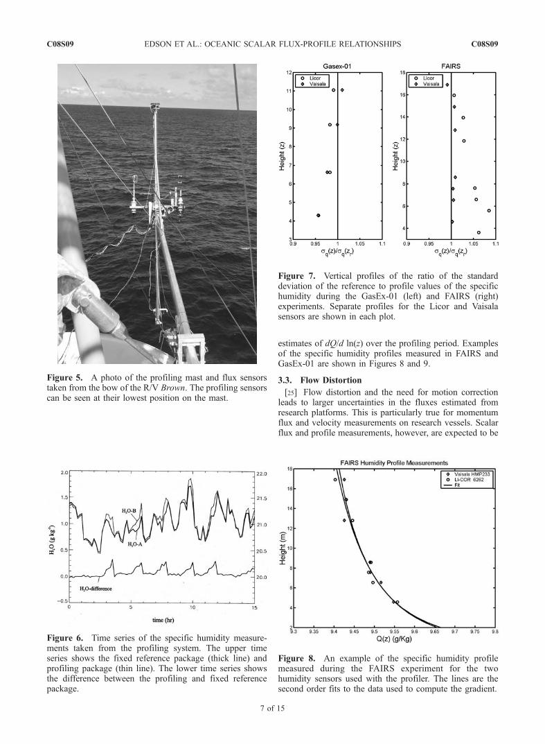
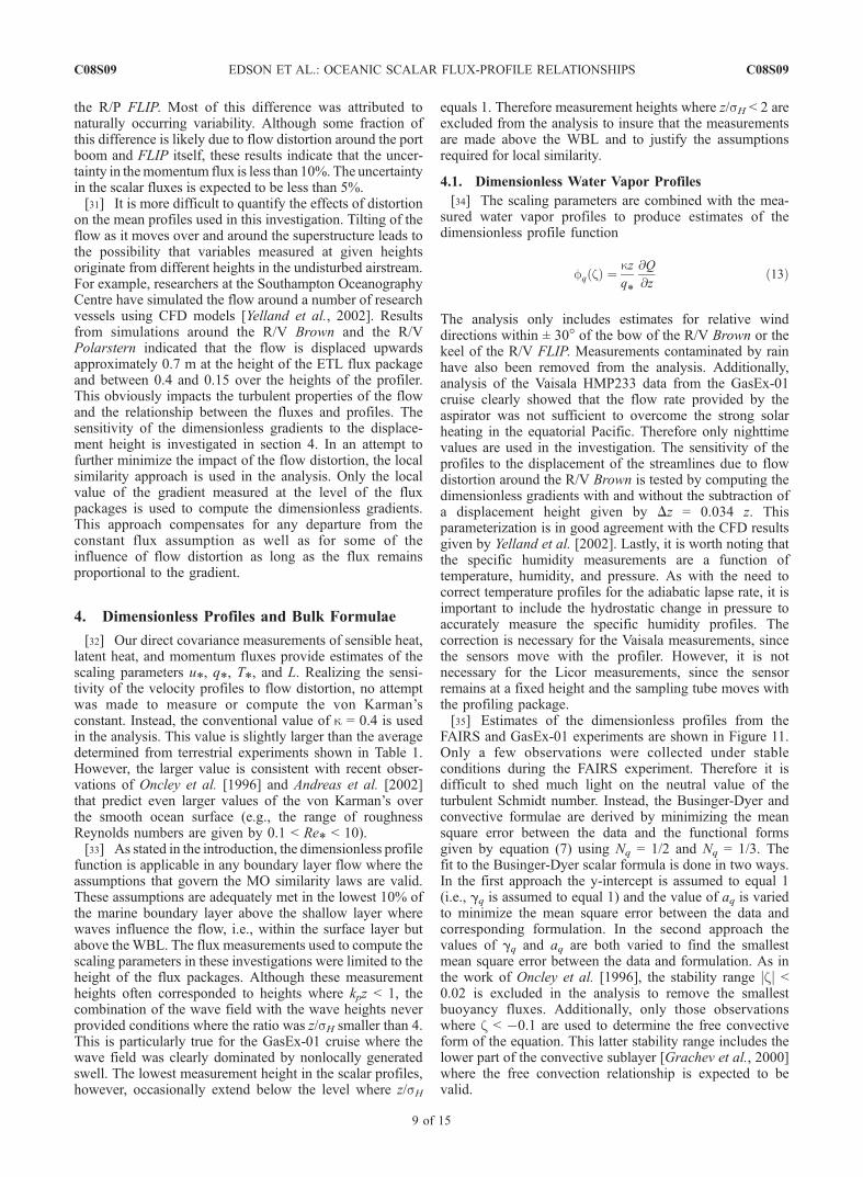
boom supported a profiling system that moved a suite ofsensors between 3 and 12 m above the mean sea level asshown in Figure 5. The sensor suite did not include ananemometer but was otherwise identical to the packageused in FAIRS. As in FAIRS, the moving sensors werereferenced against a fixed suite of sensors located at 9 m. Asingle profile took approximately 1 hour to complete.Naturally occurring temporal variability over this samplingperiod often generated larger differences than the differ-ences due to the gradient as shown in Figure 6. Most of thenaturally occurring temporal variability in water vapor wasremoved by referencing each measurement at a given heightversus a fixed sensor. The difference between the fixedand traveling sensors is shown in the lower time series inFigure 6. The results indicate that this approach removesmost of the temporal variability such that the gradient in thewater vapor profile is clearly visible. The main advantage of

Figure 1. Composite images of the experimental setupused during the Fluxes, Air-Sea Interaction, and RemoteSensing (FAIRS) experiment. The upper left image showsthe three-axis sonic anemometer-thermometer and infraredhygrometer used to compute the fluxes. The central imageshows the profiling mast as deployed on the port boom ofthe R/P FLIP. The lower left image shows the package thattraveled up and down the profiler during the experiment.

Figure 2. Time series of the fluxes derived from the directcovariance and bulk aerodynamic methods during FAIRS.The upper panel is the friction velocity derived from thestress estimates and the middle and lower panels are thelatent heat and sensible heat fluxes, respectively.

C08S09 EDSON ET AL.: OCEANIC SCALAR FLUX-PROFILE RELATIONSHIPS

5 of 15

C08S09

this approach over fixed sensors is that it reduces thecalibration errors that arise between sensors due to driftand degradation at sea.[23] This approach assumes that the temporal variability

is uniform over the measurement heights. To test thisassumption, the ratio of the standard deviation of the profileto reference specific humidity measurements over thecourse of the two experiments is shown in Figure 7. TheFAIRS results are consistent with the observation thatthe Licor measurements were substantially noisier thanthe Vaisala measurements due to difficulties with securingthe sampling tubes, particularly at the lowest levels. TheGasEx-01 measurements show less variability in bothprofiles. However, both experiments indicate that theuncertainty due to this assumption increases near the sur-face. We estimate the uncertainty due to this assumption isapproximately 5–10%.[24] The Vaisala relative humidity and temperature sen-

sors were calibrated before the cruises. A secondary in situcalibration of the profiling sensors (including the closedpath IRGAs) against the reference sensors was conductedduring postanalysis. The secondary calibration amounted toa small correction to the Vaisala sensors and removal of abias in the IRGAs. The vertical profiles were computedfrom a least squares fit to

Q z; tið Þ � Qr tið Þ½ � þ 1

N

XNi¼1

Qr tið Þ ¼ b0 þ b1 ln zð Þ þ b2 ln zð Þ½ �2

ð12Þ

where Qr and Q are the average values at the reference andprofile height z, respectively, over the sampling interval ateach height ti, and N is the total number of samplingintervals. Therefore the last term on the left-hand side is themean value of the humidity over the profiling period. Thegradient is then determined by differentiating the right-handside of equation (12) to find dQ/d ln(z). Individual profilesfrom the Licor and Vaisala sensors are used to compute two

Figure 3. The experiment setup used during the GasEx experiment aboard the R/V Ronald Brown. Themast extended 10 m forward of the bow at its closest point. The figure also shows the flux packagedeployed by National Oceanic and Atmospheric Administration Environmental Technology Laboratoryon the forward jackstaff and the infrared imagery system deployed by University of Washington AppliedPhysics Laboratory on the scaffolding.

Figure 4. As in Figure 2 for the GasEx experiment.

C08S09 EDSON ET AL.: OCEANIC SCALAR FLUX-PROFILE RELATIONSHIPS

6 of 15

C08S09

estimates of dQ/d ln(z) over the profiling period. Examplesof the specific humidity profiles measured in FAIRS andGasEx-01 are shown in Figures 8 and 9.

3.3. Flow Distortion

[25] Flow distortion and the need for motion correctionleads to larger uncertainties in the fluxes estimated fromresearch platforms. This is particularly true for momentumflux and velocity measurements on research vessels. Scalarflux and profile measurements, however, are expected to be

Figure 5. A photo of the profiling mast and flux sensorstaken from the bow of the R/V Brown. The profiling sensorscan be seen at their lowest position on the mast.

Figure 6. Time series of the specific humidity measure-ments taken from the profiling system. The upper timeseries shows the fixed reference package (thick line) andprofiling package (thin line). The lower time series showsthe difference between the profiling and fixed referencepackage.

Figure 7. Vertical profiles of the ratio of the standarddeviation of the reference to profile values of the specifichumidity during the GasEx-01 (left) and FAIRS (right)experiments. Separate profiles for the Licor and Vaisalasensors are shown in each plot.

Figure 8. An example of the specific humidity profilemeasured during the FAIRS experiment for the twohumidity sensors used with the profiler. The lines are thesecond order fits to the data used to compute the gradient.

C08S09 EDSON ET AL.: OCEANIC SCALAR FLUX-PROFILE RELATIONSHIPS

7 of 15

C08S09

less sensitive to flow distortion than the velocity measure-ments [e.g., Wyngaard, 1988; Pedreros et al., 2003]. Forthis reason this investigation focuses on dimensionlessscalar profiles. However, since flow distortion is expectedto adversely affect even the scalar flux and profile measure-ments, this section attempts to quantify the uncertainty inthese measurements using results from previous and currentinvestigations.[26] While the adverse effects of flow distortion around

the superstructure and supporting structures are unavoidableon both the R/P FLIP and R/V Brown, this effect can beminimized through careful design of the mounts and place-ment of the sensors as far away from the superstructure aspractical. For scalars, Wyngaard [1988] results indicate thatthe effect of flow distortion due to the sensor package isnegligible if CD

1/2(r/kz)1/3 � 1, where CD is the dragcoefficient and r is the size of the sensor package. Thiscondition is easily meet even a few meters above the oceansurface owing to the small size (r 0.5 m) of the sensorpackages and the reduced turbulence intensities (asreflected by CD

1/2 0.035) in the marine surface layer.[27] This criteria does not apply to the flow distortion due

to the platform superstructure. Edson et al. [1998] comparedfluxes measured on the R/V Wecoma with those computedon the R/P FLIP, which requires minimal motion correctionand is considered largely distortion-free. Their analysisindicated that the R/V Wecoma momentum fluxes were10–15% larger than those from the R/P FLIP. Aftercorrecting for motion and the systematic increase due toflow distortion, Edson et al. [1998] estimated that theuncertainty ranged from 10 to 20% for the momentumfluxes and 5 to 10% for the scalar fluxes (i.e., the uncer-tainty in u*). Pedreros et al. [2003] derived similar resultsfrom a comparison between the R/V L’Atalante and the R/PASIS (a largely distortion-free spar buoy). They concludedthat the momentum fluxes on the L’Atalante were 18%higher than ASIS, in good agreement with the Wecomaresults. In contrast, the heat fluxes between the L’Atalanteand ASIS compared extremely well, indicating that theywere less affected by flow distortion.

[28] During GasEx-01, three flux packages weredeployed aboard the R/V Brown; the two packages at theend of the bow boom are described above. The thirdpackage was deployed by the Environmental TechnologyLaboratory (ETL) on the forward jackstaff placing thesensors 8.6 m above the bow and 17.6 m above the oceansurface. The ETL velocity measurements have been cor-rected for flow distortion using results from in situ compar-isons and computational fluid dynamics (CFD) models[Yelland et al., 2002]. The ratio of the latent heat fluxes,friction velocity, and humidity scaling parameters measuredat the two vertical locations as a function of relative winddirection is shown in Figure 10. The median value of theseratios over the relative wind directions used in this analysisis 1.07, 1.05, and 1.00 for the latent heat flux, frictionvelocity, and humidity scaling velocity, respectively.[29] Some of the variability in the flux estimates is a

result of naturally occurring processes. For example, someof the difference is likely due to the expected decrease of theflux magnitude with height in a typical atmospheric bound-ary layer. However, the variation in magnitude with relativewind direction is most likely due to flow distortion, and thisvariability is approximately 10%. Of particular interest forthis investigation is the removal of the systematic differencein the humidity scaling parameter after normalization by thefriction velocity. This result suggests that any offset due toflow distortion is largely removed from the scalar compo-nent after normalization.[30] Smaller uncertainties in the flux estimates are

expected on the R/P FLIP owing to its reduced motion,smaller superstructure, and the ability to place the sensorswell away from the superstructure. Edson et al. [1998]found a 9% difference in the momentum flux measuredapproximately 3 m below and 4 m above the port boom on

Figure 9. As in Figure 8 for the GasEx experiment.

Figure 10. The ratio of the latent heat fluxes (top), frictionvelocity (middle), and specific humidity scaling parameter(bottom) measured on the bow boom at 9 m versus thevalues measured on the jackstaff at 18 m as a function of therelative wind direction. In this convention, 180 represents arelative wind direction directly on the bow (i.e., bow tostern). The data shown here represents the range of relativewind directions used in the analysis between 150 and 210.

C08S09 EDSON ET AL.: OCEANIC SCALAR FLUX-PROFILE RELATIONSHIPS

8 of 15

C08S09

the R/P FLIP. Most of this difference was attributed tonaturally occurring variability. Although some fraction ofthis difference is likely due to flow distortion around the portboom and FLIP itself, these results indicate that the uncer-tainty in themomentum flux is less than 10%. The uncertaintyin the scalar fluxes is expected to be less than 5%.[31] It is more difficult to quantify the effects of distortion

on the mean profiles used in this investigation. Tilting of theflow as it moves over and around the superstructure leads tothe possibility that variables measured at given heightsoriginate from different heights in the undisturbed airstream.For example, researchers at the Southampton OceanographyCentre have simulated the flow around a number of researchvessels using CFD models [Yelland et al., 2002]. Resultsfrom simulations around the R/V Brown and the R/VPolarstern indicated that the flow is displaced upwardsapproximately 0.7 m at the height of the ETL flux packageand between 0.4 and 0.15 over the heights of the profiler.This obviously impacts the turbulent properties of the flowand the relationship between the fluxes and profiles. Thesensitivity of the dimensionless gradients to the displace-ment height is investigated in section 4. In an attempt tofurther minimize the impact of the flow distortion, the localsimilarity approach is used in the analysis. Only the localvalue of the gradient measured at the level of the fluxpackages is used to compute the dimensionless gradients.This approach compensates for any departure from theconstant flux assumption as well as for some of theinfluence of flow distortion as long as the flux remainsproportional to the gradient.

4. Dimensionless Profiles and Bulk Formulae

[32] Our direct covariance measurements of sensible heat,latent heat, and momentum fluxes provide estimates of thescaling parameters u*, q*, T*, and L. Realizing the sensi-tivity of the velocity profiles to flow distortion, no attemptwas made to measure or compute the von Karman’sconstant. Instead, the conventional value of k = 0.4 is usedin the analysis. This value is slightly larger than the averagedetermined from terrestrial experiments shown in Table 1.However, the larger value is consistent with recent obser-vations of Oncley et al. [1996] and Andreas et al. [2002]that predict even larger values of the von Karman’s overthe smooth ocean surface (e.g., the range of roughnessReynolds numbers are given by 0.1 < Re* < 10).[33] As stated in the introduction, the dimensionless profile

function is applicable in any boundary layer flow where theassumptions that govern the MO similarity laws are valid.These assumptions are adequately met in the lowest 10% ofthe marine boundary layer above the shallow layer wherewaves influence the flow, i.e., within the surface layer butabove theWBL. The flux measurements used to compute thescaling parameters in these investigations were limited to theheight of the flux packages. Although these measurementheights often corresponded to heights where kpz < 1, thecombination of the wave field with the wave heights neverprovided conditions where the ratio was z/sH smaller than 4.This is particularly true for the GasEx-01 cruise where thewave field was clearly dominated by nonlocally generatedswell. The lowest measurement height in the scalar profiles,however, occasionally extend below the level where z/sH

equals 1. Therefore measurement heights where z/sH < 2 areexcluded from the analysis to insure that the measurementsare made above the WBL and to justify the assumptionsrequired for local similarity.

4.1. Dimensionless Water Vapor Profiles

[34] The scaling parameters are combined with the mea-sured water vapor profiles to produce estimates of thedimensionless profile function

fq zð Þ ¼ kzq*

@Q

@zð13Þ

The analysis only includes estimates for relative winddirections within ± 30 of the bow of the R/V Brown or thekeel of the R/V FLIP. Measurements contaminated by rainhave also been removed from the analysis. Additionally,analysis of the Vaisala HMP233 data from the GasEx-01cruise clearly showed that the flow rate provided by theaspirator was not sufficient to overcome the strong solarheating in the equatorial Pacific. Therefore only nighttimevalues are used in the investigation. The sensitivity of theprofiles to the displacement of the streamlines due to flowdistortion around the R/V Brown is tested by computing thedimensionless gradients with and without the subtraction ofa displacement height given by Dz = 0.034 z. Thisparameterization is in good agreement with the CFD resultsgiven by Yelland et al. [2002]. Lastly, it is worth noting thatthe specific humidity measurements are a function oftemperature, humidity, and pressure. As with the need tocorrect temperature profiles for the adiabatic lapse rate, it isimportant to include the hydrostatic change in pressure toaccurately measure the specific humidity profiles. Thecorrection is necessary for the Vaisala measurements, sincethe sensors move with the profiler. However, it is notnecessary for the Licor measurements, since the sensorremains at a fixed height and the sampling tube moves withthe profiling package.[35] Estimates of the dimensionless profiles from the

FAIRS and GasEx-01 experiments are shown in Figure 11.Only a few observations were collected under stableconditions during the FAIRS experiment. Therefore it isdifficult to shed much light on the neutral value of theturbulent Schmidt number. Instead, the Businger-Dyer andconvective formulae are derived by minimizing the meansquare error between the data and the functional formsgiven by equation (7) using Nq = 1/2 and Nq = 1/3. Thefit to the Businger-Dyer scalar formula is done in two ways.In the first approach the y-intercept is assumed to equal 1(i.e., gq is assumed to equal 1) and the value of aq is variedto minimize the mean square error between the data andcorresponding formulation. In the second approach thevalues of gq and aq are both varied to find the smallestmean square error between the data and formulation. As inthe work of Oncley et al. [1996], the stability range jzj <0.02 is excluded in the analysis to remove the smallestbuoyancy fluxes. Additionally, only those observationswhere z < �0.1 are used to determine the free convectiveform of the equation. This latter stability range includes thelower part of the convective sublayer [Grachev et al., 2000]where the free convection relationship is expected to bevalid.

C08S09 EDSON ET AL.: OCEANIC SCALAR FLUX-PROFILE RELATIONSHIPS

9 of 15

C08S09

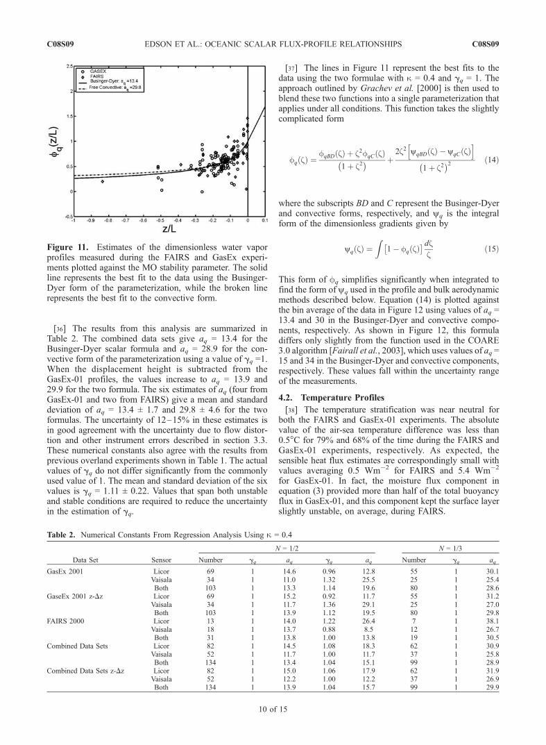
[36] The results from this analysis are summarized inTable 2. The combined data sets give aq = 13.4 for theBusinger-Dyer scalar formula and aq = 28.9 for the con-vective form of the parameterization using a value of gq =1.When the displacement height is subtracted from theGasEx-01 profiles, the values increase to aq = 13.9 and29.9 for the two formula. The six estimates of aq (four fromGasEx-01 and two from FAIRS) give a mean and standarddeviation of aq = 13.4 ± 1.7 and 29.8 ± 4.6 for the twoformulas. The uncertainty of 12–15% in these estimates isin good agreement with the uncertainty due to flow distor-tion and other instrument errors described in section 3.3.These numerical constants also agree with the results fromprevious overland experiments shown in Table 1. The actualvalues of gq do not differ significantly from the commonlyused value of 1. The mean and standard deviation of the sixvalues is gq = 1.11 ± 0.22. Values that span both unstableand stable conditions are required to reduce the uncertaintyin the estimation of gq.

[37] The lines in Figure 11 represent the best fits to thedata using the two formulae with k = 0.4 and gq = 1. Theapproach outlined by Grachev et al. [2000] is then used toblend these two functions into a single parameterization thatapplies under all conditions. This function takes the slightlycomplicated form

fq zð Þ ¼fqBD zð Þ þ z2fqC zð Þ

1þ z2� � þ

2z2 yqBD zð Þ � yqC zð Þh i

1þ z2� �2 ð14Þ

where the subscripts BD and C represent the Businger-Dyerand convective forms, respectively, and yq is the integralform of the dimensionless gradients given by

yq zð Þ ¼Z

1� fq zð Þ� � dz

zð15Þ

This form of fq simplifies significantly when integrated tofind the form of yq used in the profile and bulk aerodynamicmethods described below. Equation (14) is plotted againstthe bin average of the data in Figure 12 using values of aq =13.4 and 30 in the Businger-Dyer and convective compo-nents, respectively. As shown in Figure 12, this formuladiffers only slightly from the function used in the COARE3.0 algorithm [Fairall et al., 2003], which uses values of aq =15 and 34 in the Businger-Dyer and convective components,respectively. These values fall within the uncertainty rangeof the measurements.

4.2. Temperature Profiles

[38] The temperature stratification was near neutral forboth the FAIRS and GasEx-01 experiments. The absolutevalue of the air-sea temperature difference was less than0.5C for 79% and 68% of the time during the FAIRS andGasEx-01 experiments, respectively. As expected, thesensible heat flux estimates are correspondingly small withvalues averaging 0.5 Wm�2 for FAIRS and 5.4 Wm�2

for GasEx-01. In fact, the moisture flux component inequation (3) provided more than half of the total buoyancyflux in GasEx-01, and this component kept the surface layerslightly unstable, on average, during FAIRS.

Figure 11. Estimates of the dimensionless water vaporprofiles measured during the FAIRS and GasEx experi-ments plotted against the MO stability parameter. The solidline represents the best fit to the data using the Businger-Dyer form of the parameterization, while the broken linerepresents the best fit to the convective form.

Table 2. Numerical Constants From Regression Analysis Using k = 0.4

Data Set Sensor

N = 1/2 N = 1/3

Number gq aq gq aq Number gq aq

GasEx 2001 Licor 69 1 14.6 0.96 12.8 55 1 30.1Vaisala 34 1 11.0 1.32 25.5 25 1 25.4Both 103 1 13.3 1.14 19.6 80 1 28.6

GaseEx 2001 z-Dz Licor 69 1 15.2 0.92 11.7 55 1 31.2Vaisala 34 1 11.7 1.36 29.1 25 1 27.0Both 103 1 13.9 1.12 19.5 80 1 29.8

FAIRS 2000 Licor 13 1 14.0 1.22 26.4 7 1 38.1Vaisala 18 1 13.7 0.88 8.5 12 1 26.7Both 31 1 13.8 1.00 13.8 19 1 30.5

Combined Data Sets Licor 82 1 14.5 1.08 18.3 62 1 30.9Vaisala 52 1 11.7 1.00 11.7 37 1 25.8Both 134 1 13.4 1.04 15.1 99 1 28.9

Combined Data Sets z-Dz Licor 82 1 15.0 1.06 17.9 62 1 31.9Vaisala 52 1 12.2 1.00 12.2 37 1 26.9Both 134 1 13.9 1.04 15.7 99 1 29.9

C08S09 EDSON ET AL.: OCEANIC SCALAR FLUX-PROFILE RELATIONSHIPS

10 of 15

C08S09

[39] The small air-sea temperature difference obviouslymakes it difficult to resolve the temperature profiles, whichwere often similar in magnitude to the adiabatic lapse rate.This is illustrated in Figure 13, where the top panel repre-sents the dimensionless profile function using the absolutetemperature profiles and the bottom panel uses the potentialtemperature profiles. These plots show that the dimension-

less profiles estimates are too large when the uncorrectedtemperature profiles (i.e., without correction for the adiabaticlapse rate) are used. Nonetheless, even though these smallgradients and fluxes generate large uncertainties in theseestimates of fq(z), the cluster of points is centered aroundthe results from the humidity profiles as shown in Figure 14.However, further analysis using this data was not warrantedowing to the significant scatter and large experimentaluncertainty in these estimates.

4.3. Bulk Aerodynamic Method

[40] Perhaps the most common use of the dimensionlessprofile functions in physical oceanography and marinemeteorology is to provide indirect estimates of the fluxesthrough the bulk aerodynamic, profile, and inertial dissipa-tion methods. The bulk aerodynamic method is undoubtedlythe most commonly used approach to estimate the surfacefluxes from observations. The method relates the fluxes tothe air-sea differences in velocity, humidity, and potentialtemperature through transfer coefficients as

ts ¼ raCDU2r ð16Þ

Qe ¼ raLeCE Q zoq� �

� Q zð Þ� �

Ur ð17Þ

Qh ¼ racpCH T zoqð Þ �Q zð Þ� �

Ur ð18Þ

where CD is the drag coefficient, Ur is the wind speedrelative to the ocean surface, and CH and CE are the Stantonand Dalton numbers, respectively. Q(zoq) and T(zot) are thevalues of the specific humidity and temperature at thesurface, respectively, where zoq and zot are the thermalroughness lengths [e.g., Liu et al., 1979]. The Stanton and

Figure 12. The data shown in Figure 10 bin averaged bystability. Each bin has the same number of data points. Theerror bars represent the standard error in the measurements.The solid line represents the blended form of the dimension-less shear using the coefficients determined by the bestfits. The broken line is the blended form used in the CoupledOcean-Atmosphere Response Experiment (COARE)3.0 algorithm.

Figure 13. Estimates of the dimensionless temperature(top) and potential temperature (bottom) functions measuredduring the FAIRS and GasEx experiments plotted againstthe MO stability parameter. The lines are the same functionsshown in Figure 10.

Figure 14. A comparison of the dimensionless watervapor (bold symbols) and potential temperature profilesfrom the two experiments. The lines are the same functionsshown in Figure 10.

C08S09 EDSON ET AL.: OCEANIC SCALAR FLUX-PROFILE RELATIONSHIPS

11 of 15

C08S09

Dalton numbers can be defined in terms of the dragcoefficient and their respective scalar transfer coefficients

CH ¼ C1=2D Cq ¼ CuCq ð19Þ

CE ¼ C1=2D Cq ¼ CuCq ð20Þ

As stated above, this approach is advantageous because itallows investigators to separate the drag coefficient, whichis sensitive to both sea state and wave age, from the scalartransfer coefficients, which are expected to be lessinfluenced by the waves. Instead, these transfer coefficientsmay be influenced by additional processes such as wavebreaking and heat exchange from evaporating sea-spray.[41] The drag coefficient, Stanton number, and Dalton

number are often empirically determined as a function ofwind speed [Large and Pond, 1981; Smith, 1988; DeCosmoet al., 1996]. Another common approach is to determine thetransfer coefficients using a semiempirical method based onMO similarity theory. The semiempirical forms are derivedusing the integral form of equation (1) given by

X zð Þ ¼ X zoxð Þ þx*k

lnz

zox

�� yx

z

L

� �þ yx

zox

L

� �� �ð21Þ

where yx(zox/L)is normally ignored because it is typicallymuch smaller than the other terms. The combination ofequation (21) with equations (17) through (20) results infunctional forms of the transfer coefficients that depend onstability and the thermal roughness lengths

Cx z=zox;z� �

¼ k=gxln z

zox

� �� yx zð Þ

24

35 ð22Þ

The use of these forms of the transfer coefficient thereforerequires parameterizations of yx and zox. The integral formof the dimensionless gradient function can be found usingthe approach given by Fairall et al. [1996]. Integration ofequation (14) results in a parameterization with the correctform in the convective limit given by

yx zð Þ ¼ yxBD zð Þ þ z2yxC zð Þ1þ z2

ð23Þ

where the functions form of yxBD and yxC are given byPaulson [1970] and Fairall et al. [1996], respectively.[42] The thermal length scale is commonly parameterized

as a function of the roughness Reynold’s number [e.g., Liuet al., 1979; Fairall et al., 1996]

zoy ¼ f Reoð Þ ð24Þ

Field studies have shown that the transfer coefficients forheat and water vapor show substantial scatter and little windspeed dependence [Liu et al., 1979; Smith, 1988]. In fact,the uncertainty in field estimates of the transfer coefficientsfor temperature and humidity has resulted in the widespreaduse of laboratory-based parameterizations of zot for openocean transfer coefficient models [Liu et al., 1979;Brutsaert, 1982]. However, this is mainly due to theuncertainty in the field measurements rather than anunderstanding of the physical processes driving theexchange.[43] Accurate estimates of the sea-surface temperature

(SST) or skin temperature, T(zot), were computed usinginfrared techniques [Jessup, 2002] during the FAIRS andGasEx-01 experiments. The SST measurements are used toestimate Q(zoq) by computing the saturation value for freshwater with a correction factor of 0.97 to account for salinity[Fairall et al., 1996]. This provides an accurate estimate ofQ(zoq) without the need to model the warm layer and coolskin effects required with estimates of the sea temperaturemeasured beneath the surface.[44] These measurements are then combined with the

profile measurements to provide estimates of the thermalroughness length found by extrapolation of the adjustedprofiles to the surface values. Specifically, the linear fit ofQ(z) � Q(zq) versus ln(z) � yq (z/L) has a slope of k/q

*and a y-intercept of ln(zoq). An example of such a fit andextrapolation to the surface value is shown in Figure 15,where the actual values of Q(z) and Q(zq) are plotted toprovide a sense of the air-sea humidity difference duringGasEx-01. Values of zoq are plotted versus Reo inFigure 16, where the thermal roughness lengths arecomputed using the stability function given by equation (23)with the values of aq determined from this investigation.Individual estimates of the roughness lengths are shownin the top panel, which have been estimated with andwithout subtraction of Dz. The difference is almostundetectable in the semilogarithmic presentation. The datahave been binned into eight ranges where each range hasthe same number of data points, and the mean, median,and log-average are shown for each bin. The median andlog-average values give similar results and show goodagreement with the COARE 3.0 parameterization, i.e., the

Figure 15. An example of the semilogarithmic fit andextrapolation to the sea surface used to estimate the thermalroughness length. The yq function uses the same coeffi-cients found from the best fit analysis.

C08S09 EDSON ET AL.: OCEANIC SCALAR FLUX-PROFILE RELATIONSHIPS

12 of 15

C08S09

parameterization generally lies within the standard errorabout these estimates. The plot also shows that themedian values with and without the subtraction of Dzare very similar. There is some indication that themeasurements are slightly larger than predicted by the

parameterization. However, the large uncertainties in theseestimates require additional measurements to modify thisparameterization.

4.4. Sea State and the WBL for Scalars

[45] The setups used in FAIRS and GasEx-01 were notdesigned to investigate the role of waves on the scalarflux-profile relationships. However, the results can beused to provide evidence that the measurements weremade above the WBL for heat and mass transfer. Forexample, the difference between the individual measure-ments of kz/q*@Q/@z and the best-fit parameterization offq(z) given by equation (14) can be plotted againstseveral commonly used sea-state parameters to investigatewhether the residual is correlated with these parameters.The residual is plotted against z/sH and kpz in Figures 17and 18. The individual points and bin-averaged data inthe upper and lower panel, respectively, show little or nodependence on these wave-related parameters in theswell-dominated wave field often encountered over theopen ocean. These results support the conclusion thatthe measurements are made above the WBL for heat andmass exchange.[46] These results indicate that the turbulence responsi-

ble for transporting heat and mass is locally generated byshear and buoyancy. This is a necessary requirement forapplication of MO similarity. However, these results donot necessary imply that the scalar fluxes are uninflu-enced by waves at all heights. For example, it is wellknown that the momentum flux and u* are expected to bea function of sea state. However, normalization of thefluxes by is expected to significantly reduce the effect ofwaves on the scalar component of the flux, i.e., q* andT*. Investigations of the influence of waves on the scalarfluxes and flux profile relationship therefore require a

Figure 16. Estimates of the thermal roughness lengths forspecific humidity computed from extrapolation to thesurface values. Individual estimates of the roughnesslengths are shown in the top panel estimated with andwithout subtraction of Dz. The bottom panel shows bin-averaged estimates where the symbols represent theaverage, median, and log-average values as indicated andthe error bars are the standard error about the median value.The error bars for points 1 and 6 are less than ±2. The solidline is the COARE 3.0 parameterization.

Figure 17. The difference between the individual mea-surements shown in Figure 10 and the best fit parameter-ization shown in Figure 11 versus the ratio of themeasurement height to significant wave height z/sH.

Figure 18. The difference between the individual mea-surements shown in Figure 10 and the best fit parameter-ization shown in Figure 11 versus the dimensionless height,kpz, which equals the ratio of the measurement height towave length times 2p.

C08S09 EDSON ET AL.: OCEANIC SCALAR FLUX-PROFILE RELATIONSHIPS

13 of 15

C08S09

setup with profiles and fluxes measured much closer tothe air-sea interface.

5. Conclusions

[47] Our open ocean estimates are in good agreementwith commonly used parameterizations based on overlandmeasurements. This indicates that the MO similarityfunctions are applicable over the ocean where appropriate,i.e., in the surface layer above the WBL where thestructure of the turbulence is dominated by the relativeimportance of mechanical (i.e., wind shear) versus ther-mal forcing. In the analysis a value of aq = 13.4 givesgood agreement with the data using Businger-Dyer formsof the equations in near-neutral conditions. Using theapproach outlined by Fairall et al. [1996] and Grachevet al. [2000], the blended parameterization shows goodagreement with the data, using a value of aq = 30 for theconvective component of the dimensionless gradient. Theresulting functions are not significantly different fromthe latest parameterizations of the dimensionless gradientsused in the COARE 3.0 algorithm [Fairall et al., 2003],and the results are in good agreement with the consensusvalues found from previous overland experiments shownin Table 1.[48] Although the fluxmeasurementsweremade at a single

elevation and local similarity scaling is applied, the goodagreement implies that MO similarity is valid within themarine atmospheric surface layer. The results also indicatethat the scalar fluxes are not influenced by wave-inducedeffects at the measurement heights, i.e., the measurementswere taken above the WBL for scalars. As a result, thedimensionless gradients based on MO similarity can be usedto compute scalar fluxes in the region of the surface layerabove the scalar WBL. This region corresponds to typicalmeasurement heights aboard research vessels. To make thissame claim for buoys and other platforms that place thesensors closer to the surface would obviously require profileand flux measurements closer to the surface.[49] The thermal roughness lengths determined from

extrapolation of the semilogarithmic profiles to the surfacevalues are also in good agreement with the COARE 3.0algorithm. There is some indication that the COARE 3.0algorithm overestimates the values of the thermal roughnesslengths at low Reynold’s numbers. However, the largeuncertainty in this extrapolation caused by the accumulatedeffect of the various experimental errors makes it difficult toquantify this observation. The reduction of this uncertaintyis an objective of the recently conducted Coupled BoundaryLayers and Air-Sea Transfer (CBLAST) experiment at theMartha’s Vineyard Coastal Observatory.

[50] Acknowledgments. The FAIRS work was supported by theOffice of Naval Research grant N00014-00-1-0403 while the GasEx workwas supported by the National Science Foundation grant OCE-9986724.The authors wish to recognize the crews of the R/P FLIP and NOAA ShipRonald H. Brown for their outstanding efforts. We would like to thankSteve Faluotico, Sean McKenna, and Glenn McDonald from WHOI fortheir help in developing and maintaining the flux-profile system during theFAIRS and GasEx cruises. We would like to thank Andrew Jessup fromUW/APL and Brian Ward from NOAA/AOML for their assistance with thesea surface and bulk temperature measurements. Finally, we would like tothank Sheila Hurst for her editorial assistance. This is Woods HoleOceanographic Institution contribution 10925.

ReferencesAndreas, E. L., and K. A. Emanuel (2001), Effects of sea spray on tropicalcyclone intensity, J. Atmos. Sci., 58, 3741–3751.

Andreas, E. L., K. J. Claffey, C. W. Fairall, P. S. Guest, R. E. Jordan, andP. O. G. Persson (2002), Evidence from the atmospheric surface layer thatthe von Karman constant isn’t, in Fifteenth Symposium on BoundaryLayers and Turbulence, pp. 418–421, Am. Meteorol. Soc., Boston.

Badgley, F. I., and C. A. Paulson (1972), Profiles of wind, temperature andhumidity over the Arabian Sea I: The observations, Int. Indian OceanExped. Meteor. Mongr., 6, 3–29.

Brutsaert, W. (1982), Evaporation into the Atmosphere, 299 pp., D. Reidel,Norwell, Mass.

Businger, J. A. (1988), A note on the Businger-Dyer profiles, BoundaryLayer Meteorol., 42, 145–151.

Businger, J. A., J. C. Wyngaard, Y. Izumi, and E. F. Bradley (1971), Flux-profile relations in the atmospheric surface layer, J. Atmos. Sci., 28, 181–189.

Carl, M. D., T. C. Tarbell, and H. A. Panofsky (1973), Profiles of wind andtemperature from towers over homogeneous terrain, J. Atmos. Sci., 30,788–794.

DeCosmo, J., K. B. Katsaros, S. D. Smith, R. J. Anderson, W. A. Oost,K. Bumke, and H. Chadwick (1996), Air-sea exchange of water vaporand sensible heat: The Humidity Exchange over the Sea (HEXOS)results, J. Geophys. Res., 101, 12,001–12,016.

Dyer, A. J., and E. F. Bradley (1982), An alternative analysis of flux-gradient relationships at the 1976 ITCE, Boundary Layer Meteorol.,22, 3–19.

Dyer, A. J., and B. B. Hicks (1970), Flux-gradient relationships in theconstant flux layer, Q. J. R. Meteorol. Soc., 96, 715–721.

Edson, J. B., and C. W. Fairall (1998), Similarity relationships in the marinesurface layer, J. Atmos. Sci., 55, 2311–2328.

Edson, J. B., A. A. Hinton, K. E. Prada, J. E. Hare, and C. W. Fairall(1998), Direct covariance flux estimates from mobile platforms at sea,J. Atmos. Ocean. Technol., 15, 547–562.

Fairall, C. W., J. D. Kepert, and G. J. Holland (1994), The effect of seaspray on surface energy transports over the ocean, Global Atmos. OceanSys., 2, 121–142.

Fairall, C. W., E. F. Bradley, D. P. Rogers, J. B. Edson, and G. S. Young(1996), Bulk parameterization of air-sea fluxes for TOGA COARE,J. Geophys. Res., 101, 3747–3764.

Fairall, C. W., E. F. Bradley, J. E. Hare, A. A. Grachev, and J. B. Edson(2003), Bulk parameterization of air-sea fluxes: Updates and verificationfor the COARE algorithm, J. Clim., 16, 571–591.

Frenzen, P., and C. A. Vogel (1992), The turbulent kinetic energy budget inthe atmospheric surface layer: A review and an experimental reexamina-tion in the field, Boundary Layer Meteorol., 60, 49–76.

Frenzen, P., and C. A. Vogel (2001), Further studies of atmospheric turbu-lence in layers near the surface: Scaling the TKE budget above the rough-ness sublayer, Boundary Layer Meteorol., 99, 173–206.

Grachev, A. A., C. W. Fairall, and E. F. Bradley (2000), Convective profileconstants revisited, Boundary Layer Meteorol., 94, 495–515.

Gurvich, A. S. (1965), Vertical temperature and wind velocity profiles inthe atmospheric surface layer, Izv. Acad. Sci. USSR Atmos. OceanicPhys., Engl. Transl., 1, 31–36.

Hare, J. E., T. Hara, J. B. Edson, and J. M. Wilczak (1997), A similarityanalysis of the structure of air flow over surface waves, J. Phys. Ocean-ogr., 27, 1018–1037.

Hogstrom, U. (1988), Non-dimensional wind and temperature profiles in theatmospheric surface layer: A re-evaluation, Boundary Layer Meteorol.,42, 55–78.

Hristov, T. S., S. D. Miller, and C. A. Friehe (2003), Dynamical coupling ofwind and ocean waves through wave-induced air flow, Nature, 422, 55–58.

Janssen, P. A. E. M. (1989), Wave induced stress and the drag of the airflow over sea waves, J. Phys. Oceanogr., 19, 745–754.

Janssen, P. A. E. M. (1999), On the effect of ocean waves on the kineticenergy balance and consequences for the inertial dissipation technique,J. Phys. Oceanogr., 29, 530–534.

Jessup, A. T. (2002), Autonomous shipboard infrared radiometer system forin situ validation of satellite SST, Proc. SPIE, 4814, 222–229.

Large, W. G., and S. Pond (1981), Open ocean momentum flux mea-surements in moderate to strong winds, J. Phys. Oceanogr., 11, 324–336.

Liu, W. T., K. B. Katsaros, and J. A. Businger (1979), Bulk parameteriza-tion of air-sea exchanges of heat and water vapor including the molecularconstraints at the interface, J. Atmos. Sci., 36, 1722–1735.

Mahrt, L. (1998), Stratified atmospheric boundary layers, Boundary LayerMeteorol., 90, 375–396.

Makin, V. K. (1998), Air-sea exchange of heat in the presence of windwaves and spray, J. Geophys. Res., 103, 1137–1152.

C08S09 EDSON ET AL.: OCEANIC SCALAR FLUX-PROFILE RELATIONSHIPS

14 of 15

C08S09

Makin, V. K., and C. Mastenbroek (1996), Impact of waves on air-seaexchange of sensible heat and momentum, Boundary Layer Meteorol.,79, 279–300.

Makin, V. K., V. N. Kudryavtsev, and C. Mastenbroek (1995), Drag of thesea surface, Boundary Layer Meteorol., 73, 159–182.

Miller, S. D., C. A. Friehe, T. S. Hristov, and J. B. Edson (1997), Windand turbulence profiles in the surface layer over the ocean, in TwelfthSymposium on Boundary Layers and Turbulence, pp. 308–309, Am.Meteorol. Soc., Boston.

Miyake, M., M. Donelan, G. McBean, C. Paulson, F. Badgley, andE. Leavitt (1970), Comparison of turbulent fluxes over water determinedby profile and eddy correlation techniques, Q. J. R. Meteorol. Soc., 96,132–137.

Oncley, S. P., C. A. Friehe, J. C. LaRue, J. A. Businger, E. C. Itsweire, andS. S. Cheng (1996), Surface-layer fluxes, profiles, and turbulence mea-surements over uniform terrain under near-neutral conditions, J. Atmos.Sci., 53, 1029–1044.

Panofsky, H. A., A. K. Blackadar, and G. E. McVehil (1960), The diabaticwind profile, Q. J. R. Meteorol. Soc., 86, 495–503.

Paulson, C. A. (1970), Mathematical representation of wind speed andtemperature profiles in the unstable atmospheric surface layer, J. Appl.Meteorol., 9, 857–861.

Paulson, C. A., M. Miyake, and F. I. Badgley (1972a), Profiles of wind,temperature and humidity over the Arabian Sea II: An analysis, Intern.Indian Ocean Exped. Meteor. Mongr., 6, 33–62.

Paulson, C. A., E. Leavitt, and R. G. Fleagle (1972b), Air-sea transfer ofmomentum, heat and water determined from profile measurements duringBOMEX, J. Phys. Oceanogr., 2, 487–497.

Pedreros, R., G. Dardier, H. Dupuis, H. C. Graber, W. M. Drennan, A. Weill,C. Guerin, and P. Nacass (2003), Momentum and heat fluxes via the eddycorrelation method on the R/V L’Atalante and an ASIS buoy, J. Geophys.Res., 108(C11), 3339, doi:10.1029/2002JC001449.

Pond, S., G. T. Phelps, J. E. Paquin, G. McBean, and R. W. Stewart (1971),Measurements of the turbulent fluxes of momentum, moisture and sen-sible heat over the ocean, J. Atmos. Sci., 28, 901–917.

Poulos, G. S., et al. (2002), CASES-99: A comprehensive investigation ofthe stable nocturnal boundary layer, Bull. Am. Meteorol. Soc., 83, 555–581.

Smedman, A., U. Hogstrom, H. Bergstrom, A. Rutgersson, K. K. Kahma,and H. Pettersson (1999), A case study of air-sea interaction during swellconditions, J. Geophys. Res., 104, 25,833–25,851.

Smith, S. D. (1988), Coefficients for sea surface wind stress, heat flux, andwind profiles as a function of wind speed and temperature, J. Geophys.Res., 93, 15,467–15,472.

Stull, R. B. (1988), An Introduction to Boundary Layer Meteorology, 666pp., Kluwer Acad., Norwell, Mass.

Vickers, D., and L. Mahrt (1999), Observations of non-dimensional windshear in the coastal zone, Q. J. R. Meteorol. Soc., 125, 2685–2702.

Wyngaard, J. C. (1973), On surface layer turbulence, in Workshop onMicrometeorology, edited by D. A. Haugen, pp. 101–149, Am. Meteorol.Soc., Boston.

Wyngaard, J. C. (1988), The effects of probe-induced flow distortion onatmospheric turbulence measurements: Extension to scalars, J. Atmos.Sci., 45, 3400–3412.

Yaglom, A. M. (1977), Comments on wind and temperature flux-profilesrelationships, Boundary Layer Meteorol., 11, 89–102.

Yelland, M. J., B. I. Moat, R. W. Pascal, and D. I. Berry (2002), CFD modelestimates of the airflow distortion over research ships and the impact onmomentum flux measurements, J. Atmos. Oceanic Technol., 19, 1477–1499.

�����������������������J. B. Edson and J. A. Ware, Woods Hole Oceanographic Institution,

98 Water Street, Woods Hole, MA 02543, USA. ( jedson@whoi.edu;jware@whoi.edu)J. E. Hare, Environmental Technologies Laboratory, National Oceanic

and Atmospheric Administration, 325 Broadway R/ETL, Boulder, CO80305-3328, USA. ( jeff.hare@noaa.gov)W. R. McGillis, Geochemistry Division, Lamont-Doherty Earth

Observatory, Columbia University, 208 Geoscience, 61 Route 9W, P. O.Box 1000, Palisades, NY 10964-8000, USA. (mcgillis@ldeo.columbia.edu)C. J. Zappa, Ocean and Climate Physics Division, Lamont-Doherty Earth

Observatory, Columbia University, 204D Oceanography, 61 Route 9W, P. O.Box 1000, Palisades, NY 10964-8000, USA. (zappa@ldeo.columbia.edu)

C08S09 EDSON ET AL.: OCEANIC SCALAR FLUX-PROFILE RELATIONSHIPS

15 of 15

C08S09