Scalable methodology for the photovoltaic solar energy potential assessmentbased on available roof surface area: application to Piedmont Region (Italy)

Luca Bergamasco, Pietro Asinari

Department of Energetics, Politecnico di Torino,Corso Duca degli Abruzzi 24, Torino, Italy

Abstract

During the last few years the photovoltaic energy market hasseen an outstanding growth. According to the newDirective on renewable energies of the European Commission(2009/28/EC), the European Union should reach a 20%share of the total energy consumption from renewable sources by 2020. The national overall targets impose for Italya 17% renewable share, in case of failure the gap would be filled by importation of renewable energy from non-UEcountries. The abitious national targets and thus the continuously increasing interest on renewable fuels, requiresimple but reliable methods for the energy potential assessment over large-scale territories. Considering roof-topintegrated PV systems, the assessment of the PV energy potential passes through the evaluation of the roof surfacearea available for installations. In the present paper a methodology for estimating the PV solar energy potential ispresented, together with its application to Piedmont Region (North-Western Italy). The roof area suitable for solarapplications, is calculated through the analysis of available GIS data. The solar radiation maps are taken from thedatabase of the Joint Research Centre of the European Commission. Different solar energy exploitation scenarios areproposed with the relative perspective results and confidence interval. Further developments and applications of thepresented methodology are finally discussed.

Keywords: Photovoltaic; Roof-top PV systems; Renewable Energy; GIS

Nomenclature

N Number of . . . . . . . . . . . . . . . . . [ − ]

S Surface. . . . . . . . . . . . . . . . . . . [ m2 ]

P Population . . . . . . . . . . . . . . . . . [ − ]

D Density . . . . . . . . . . . . . . . . . . . [ ·/km2 ]

C Coefficient . . . . . . . . . . . . . . . . . [ − ]

η Efficiency. . . . . . . . . . . . . . . . . . [ − ]

µ Exp. distribution rate parameter. . . . [ − ]

H Global irradiation . . . . . . . . . . . . [ Wh/m2 ]

T Temperature. . . . . . . . . . . . . . . . [ ◦C ]

Π Electric energy potential . . . . . . . . [ Wh ]

Subscripts & Superscripts

inhab Inhabitants

m Mean

tot Total

avail Available

bui Building

res Resident, residential

ind Industrial

mun Municipality

pro Province

pop Population

mod Module

amb Ambient

MC Mono-crystalline

PC Poly-crystalline

T F Thin Film

Abbreviations

GIS Geographic Information System

BIPV Building integrated PV system

EEA European Environment Agency

CTRN Numerical Technical Regional Map

VMAP Vector Map

DEM Digital Elevation Model

ES RA European Solar Radiation Atlas

IS T AT National Institute for Statistics

HVAC Heating Ventil. and Air Cond. systems

S TC Standard Test Conditions

AM Air mass coefficient

Preprint submitted to Solar Energy September 18, 2010

1. Introduction

The interest on renewable energies is growing day byday, as fossil fuels become always more expensive anddifficult to find. Furthermore, the latest environmentaldisasters caused by the oil drilling and transportation,have further focused the attention of the entire worldon the risks connected to fossil fuels. In the last April2010, the explosion and sinking of theDeepwater Hori-zonoil rig in the Gulf of Mexico, and the start of thesubsequent massive oil leak, is a clear example. Duringthe last years, many attempts have been made to containand control the scale of the environmental disasters, butthe common sensation that fossil resources are “rapidly”going towards the end is widespreading. One of most in-teresting, among the“green resources”, is the solar en-ergy. The employment of the solar radiations has a widerange of applications, nevertheless the interest of so-lar engineering is mainly focused on thermal processesand photovoltaic applications. Particularly, taking intoaccount the photovoltaic solar energy conversion, thebuilding-integrated PV systems (BIPV) hold an impor-tant slice of the energy market (besides other commonapplications, i.e.PV farms). Integrated systems shouldbe in general preferred to massive installations, for arational use of the natural resources. In Italy, the con-tinuous and uncontrolled installation of PV farms overthe territory (highly profitable due to the economic in-centives (Conto Energia 2010, [1])), is indeed jeopar-dizing the natural landscape and occupying more andmore agricultural terrains. The increasing rate of theseinstallations and the subsequent consequences are draw-ing the attention of the public opinion and are cause ofalarm. In Italy, the large exploitation of the photovoltaicsolar energy is at the beginning and actually there existno regulation of the PV installations. The number of in-stallations in Piedmont is growing insomuch as in July(2010) the Regional Council has approved a draft law toregulate the land use and to accommodate photovoltaicsystems on the ground (Regional Council of Piedmontwebsite [2]). This moratorium against the photovoltaicdisfiguring, has been thought to both regulate the instal-lations and promote the BIPV systems. The energy pol-icy of the actual administration indeed foresees to moti-vate the installations on buildings or anyhow on alreadycompromised marginal areas.The incentive to the large scale utilization of buildingintegrated modules however supposes the knowledge ofthe technical and economic territorial potential. Severalworks have been carried out on building integrated PVsystem installations (Castro et al. [3], Sorensen [4]), butgenerally the available roof surface area is assumed to

(a)

(b)

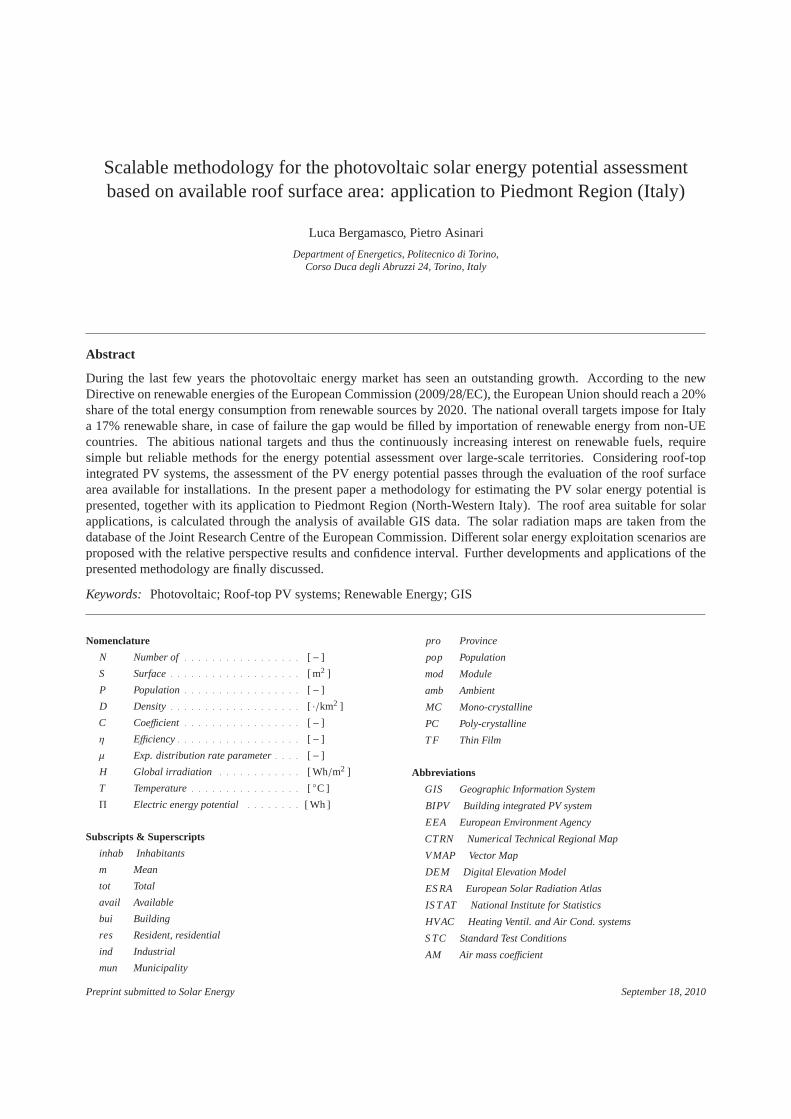
Figure 1: Subdivision of the electric power production [%] by differ-ent module technology (a) and different system-integration (b) overPiedmont Region in 2009 [10].

be an input. Furthermore, the detail of the available sur-face for PV installations is thebuilt-up area, evaluatedthrough maps of the land use (i.e. Corine Land Cover,of the European Environment Agency (EEA website[5])). This lack of methodology for the assessmentof the available roof surface area, has been partiallyfilled by some recent papers. A first scalable method-ology for the roof surface assessment based on crossed-processing and sampling of various GIS data has beenproposed together with its application to Spain in 2008(Izquierdo et al. [6]). Very recent papers discuss similarmethodologies and their relative applications to differ-ent geographical regions (Kabir et al. [7], Wiginton etal. [8]). The increasing literature on the topic reveals thegrowth of interest for the widespread exploitation of thesolar power by means of building-integrated systems.In Italy, in 2009, the total electrical energy consump-tion has been of about 320 TWh ([9],[10]), on the otherhand the total production has been of about 275 TWh,corresponding to a 14% deficit ca. The paucity of theproduction has been balanced through importation fromabroad. The only Piedmont Region in 2009 has seena production of 24.5 TWh ca. against a demand of 26

2

TWh ca. (deficit of 6% ca.). Considering the only pho-tovoltaic production, Piedmont produced 50.2 GWh,corresponding to 7.5% ca. of the total photovoltaic pro-duction in Italy. The energy production is subdividedon different module technologies and different kind ofinstallations/integration1. (Fig. 1(a), 1(b)). It is im-portant to notice that in the only Piedmont, the num-ber of installations and the installed power in 2009 hasbeen more than twice that of 2008 (respectively+118%and+149%), [10]. The present paper deals with thePV solar potential assessment over the Piedmont re-gion through the evaluation of the roof surface availablefor grid connected building-integrated PV installations(BIPV). For the sake of clearness, the term BIPV gen-erally refers to roofs and facades, in the paper we useit to refer to roof-top integrated PV systems only. Thework is organized as follows: the general outlines of themethodology are first presented. Subsequently, the pro-cedure for the assessment is discussed in detail togetherwith the various data processing. The results are pre-sented progressively: from the municipal to the regionalscale. Different scenarios for the solar energy exploita-tion are presented together with their confidence inter-val and finally, the conclusions on the present work aredrawn and perspective developments of the methodol-ogy are proposed.

2. Methodology

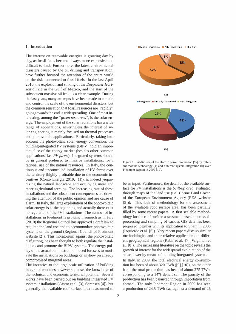
The assessment of the photovoltaic solar energy po-tential requires the evaluation of thephysical potential(useful solar radiation),geographical potential(roofsurface available) andtechnical potential(PV systemefficiency). The estimated theoretical PV potential isachieved proceeding through a hierarchical assessmentmethodology (Fig. 2). Generally, in large scale analy-sis like this, a certain level of approximation has alwaysto be accepted, thus the effort is to be done to containthe errors as much as possible, in order to achieve re-liable results. The evaluation of the various potentialsrequires to take into account a wide range of differentparameters. In the present study, it has been decidedto counter the risk of misleading results evaluating dif-ferent scenarios for each uncertainty, in a sort of para-metrical study. The initial stage of the analysis, corre-sponding to the collection of the various data is of fun-damental importance as the accuracy of the final results

1The level of integration of the PV modules is generally referred tothree main typologies:non-integrated, for ground-mounted systems(i.e. PV farms),partially-integratedif the systems are intallated onbuildings by means of additional structures,integratedif the modulesare intallated directly on building features (i.e. roofs, facades)

Figure 2: Scheme of the hierarchical methodology: the assessmentforesees the estimation of the physical, geographical and technical po-tential (energy exploitation). The theoretical PV potential is achievedaggregating the data obtained through the various levels.

depends in great measure on the precision of the originaldata (as well as on the accuracy of the analysis and onthe number of affecting parameters taken into account).A review of the available data necessary for the analy-sis has allowed an overview on the maximum precisionachievable and on the sources of the various data types.In the matter of solar radiation data, it has been decidedto refer to the maps provided by the Joint Research Cen-tre of the European Commission ([16]) (freely availablefor public use). The geographical and cadastral anal-ysis is carried out basing on the Numerical TechnicalRegional Map of Piedmont CTRN (Carta Tecnica Re-gionale Numerica). The update of the sections of themap is different over the region, the newest (current)version presents updates from 1991 to 2005. This is ac-tually the most precise territorial data available and suit-able for a large scale processing. For the sake of clar-ity, it has to be told that in Italy, all the cadastral dataare held at the municipal level by the local cadastres.There have not been unification of the cadastral data athigher level until now and furthermore, all the data havenot been computerized yet. There are nevertheless someprojects, currently ongoing, aiming to digitalize and as-sociate the cadastral data to the numerical maps. Sucha document would allow the possibility to have all thecadastral information associated to the entities presentin the numerical maps (i.e. height of buildings, numberof resident persons per building, etc.).All the analysis on the maps are performed in a commer-cial GIS software, ESRI ArcGIS 9.3. The data is suc-cessively exported for the processing, which has been

3

performed in MATLAB.

2.1. Solar radiation data

The solar radiation maps for Europe are freely avail-able on the website of the Joint Research Centre (JRC)of the European Commission ([16]). The solar radia-tion database has been developed from the climatologicdata available in theEuropean Solar Radiation Atlas,ESRA(ESRA website [15]), homogenized for Europe.The algorithm used to build the database, accounts forbeam, diffuse and reflected components of solar irradi-ation. Basically, the irradiation is computed by integra-tion of the irradiance values measured at imposed timeintervals during the day. For each time interval the ef-fect of sky obstruction (shadowing by local terrain fea-tures) is computed by means of the Digital ElevationModel (DEM). For the sake of completeness, the calcu-lation steps in the construction of the model are brieflyreported hereafter, for the details on the algorithm referto M. Suri et al. ([11]), M. Suri and Hofierka ([12]),M. Suri et al. ([13]). The model has been developedthrough the following steps:

1. computation of clear-sky global irradiation on ahorizontal surface;

2. calculation and spatial interpolation of clear-skyindex and computation of raster maps of global ir-radiation on a horizontal surface;

3. computation of the diffuse and beam componentsof overcast global irradiation and raster maps ofglobal irradiation on inclined surfaces;

4. accuracy assessment and comparison withESRAinterpolated maps.

On the website it is also possible to interrogate an in-teractive tool, the Photovoltaic Geographical Informa-tion System (PVGIS), and to obtain the solar radia-tion (kW/m2) and the photovoltaic electricity potential(kWh) in a certain location (and for an assigned in-stalled peak power), calculated on the basis of the de-sired parameters (i.e. module technology, mounting op-tions, tracking options, etc.). The utility provides dailyand monthly mean values and the yearly sum. Thedatabase has already been used to analyse regional andnational solar energy resource and to assess the photo-voltaic (PV) potential in European Union member states(MarcelSuri et al., [14]). For the purpose of the presentstudy, in order to obtain the solar radiation data at themunicipal detail, the raster maps are the most suitabletool. Among the available maps on the website, the fol-lowing are taken into account in the present paper:

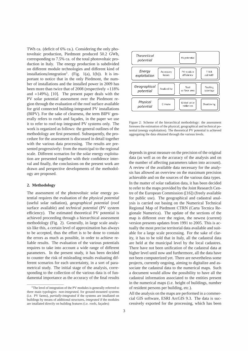
Figure 3: Yearly sum of global irradiation on the Piedmont region[kWh/m2]. The colors refer to the mean global radiation per munici-pality. These values are the interpolated among all the cell-values ofthe solar radiation map falling within the municipality.

• yearly sum of global irradiation on optimally-inclined surface (kW/m2);

• optimum inclination angle of equator-facing PVmodules to maximise yearly energy yields (◦).

The raster maps are in format ESRI ascii grid, andthe original map projection is geographic, ellipsoidWGS84. The rasters cover the extent within the fol-lowing bounds: North 72◦ N, South 32◦30’ N, West27◦ W, East 45◦ E. Each map consists of 474 rows and864 columns, for a total of 409536 cells. The grid cellsize has a resolution of 5 arc-minutes (corresponding to0.083333◦), obtained aggregating the original data with1 km resolution. All the raster maps have been vector-ized and the geo-reference system (and projection) hasbeen modified in order to match that of the Piedmontvector map. Each map has been thus overlayed to thePiedmont numerical map and clipped by the regionalborders (Fig. 3). Each data layer (solar radiation andoptimum inclination angles) has been joined to the Pied-mont vector map assigning to each municipality the cor-responding property. Particularly, the interpolated valueof the pixels within the municipality is taken.

4

(a) (b)

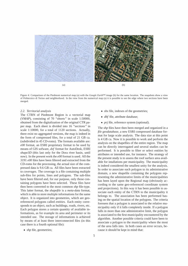
Figure 4: Comparison of the Piedmont numerical map (a) with theGoogle Earth™ image (b) for the same location. The snapshots show a viewof Politecnico di Torino and neighborhood. In the view from the numerical map (a) it is possible to see the edge where two sections have beenmerged.

2.2. Territorial analysisThe CTRN of Piedmont Region is a vectorial map(VMAP), consisting of 70“sheets” in scale 1:50000,obtained from the digitalization of the original CTR pa-per map. Each sheet is divided into 16“sections” inscale 1:10000, for a total of 1120 sections. Actually,there exist no aggregated versions, the map is indeed inthe form of compressed files, for a total of 21 GB ca.(subdivided in 45 CD-roms). The formats available are:e00 format, an ESRI proprietary format to be used bymeans of GIS sofware,dxf format for AutoDesk, ESRIshape3D(this last only for the Dora river basin, untilnow). In the present work thee00format is used. All the3191e00files have been filtered and extracted from theCD-roms for the processing, the actual size of the com-pressed data is 9.6 GB ca. All files have been extractedto coverages. The coverage is a file containing multiplesub-files for points, lines and polygons. The sub-fileshave been filtered and, for our purpose, only those con-taining polygons have been selected. These files havethen been converted to the most commonshpfile-type.This latter format, theshapefileis a meta-dataformat,which is able to store multiple informations for the sameobject. It is organized into geometries, which are geo-referenced polygons calledentities. Each entity corre-sponds to an object, such as buildings, roads, rivers, etc.Each polygon stores a certain quantity of available in-formations, as for example its area and perimeter or itsintended use. The storage of informations is achievedby means of at least three interconnected files (in thiscase there is a fourth optional file):

• shpfile, geometries;

• shxfile, indexes of the geometries;

• dbf file, attribute database;

• prj file, reference system (optional).

Theshpfiles have then been merged and organized in afile geodatabase, a new ESRI compressed database for-mat for large scale analysis. The data size at this pointis 4 GB ca. Now it is possible to work and perform theanalysis on the shapefiles of the entire region. The mapcan be directly interrogated and several studies can beperformed. It is possible to filter or select entities byattributes or intended use, for instance. The strategy ofthe present study is to assess the roof surface area avail-able for intallations per municipality. The municipalityis indeed considered the smallest unity for the analysis.In order to associate each polygon to its administrativedomain, a new shapefile containing the polygons rep-resenting the administrative limits of the municipalitieshas been layed upon the Regional map (obviously ac-cording to the same geo-referenced coordinate systemand projections). In this way it has been possible to as-sociate each entity of the CTRN to the municipality itbelongs to. The association has been performed bas-ing on the spatial location of the polygons. The criteriaforesees that a polygon is associated to the relative mu-nicipality only if it falls completely inside. If a polygonfalls in more than one administrative limit, the polygonis associated to the first municipality encountered by thealgorithm. Another possible criteria could have been toassociate a polygon to the municipality where the mostof the area falls into. In both cases an error occurs, be-cause it should be kept in mind that:

5

• the shape of the polygons representing the admin-istrative limits is slightly simplified;

• an ambiguous building (falling on the administra-tive limit), in the reality, is not necessarily assignedto a certain municipality only basing on the spatiallocation;

• the obtained data cannot be verified, as neither thelocal administrations nor the cadastre, systemati-cally provide this kind of informations.

The entity of the error due to the association algorithmwill be discussed in the section dedicated to the method-ologic uncertainties. After the association of the poly-gons to the municipalities, the entities have been fil-tered to calculate the number of residential and indus-trial buildings per municipality and the total roof sur-face area available. A brief clarification on the term“building” is mandatory. In the paper this term refers toa polygon characterized by a certain intended use (i.e.groups of adjacent residential or industrial structures).

2.3. Residential and industrial roofing

2.3.1. ResidentialIn Italy, especially in the north, the most employed rooftypology is the double-pitched (in the southern regionsflat roofs are also common). Actually, there exist nodata about the roof-type distribution. Here we assumethat the representative residential roofing typology overthe Piedmont Region is double-pitched (Fig. 5(a)). Theslope of the pitch is usually calculated according tothe maximum theoretical snow-load (besides the roof-ing material). The slope of the roofs is indeed steeperin the mountains. In Piedmont the slope of the pitchescan be assumed to range between 30 and 45% (17 to24◦ ca.). This consideration allow to calculate the effec-tive roof surface area. It should indeed be noticed thatthe building areas extrapolated from the CTRN are the2D projections of the real roof surface. These areas arehence supposed to be corrected by their own slope. Weassume a characteristic inclination angle for residentialroofing of 20◦ (θres = 20◦), and correct the area by acos(θres) factor. If we then assume that, given the slopeof the pitched-roof, the fixed installation is realized sothat the best inclination angle, ortilt angle (angle of in-clination of the array from horizontal, 0◦ = horizontal,90◦ = vertical, Fig. 5(b)) is achieved (by means of ap-posite supports), the solar radiation exploitation is max-imized.It should be reminded that an increased tilt will favourthe power output in the winter months, which is often

(a)

(b)

Figure 5: Schematic example of the representative roof typologies forresidential and industrial buildings in Piedmont with roof-top inte-grated PV installations (a). Definition of thetilt andazimuthanglesfor PV applications (b).

desired for solar water heating instead, and a decreasedtilt will favor power output in summer months. The op-timal installation angle is a mean value, calculated tomaximize the yearly energy yield. Another key factorto take into account in order to get the highest energyproduction from a photovoltaic system within a set ge-ographic area has to do with maximizing the exposureto direct sunlight. It is necessary to avoid shade and ex-pose the modules towards the sun, therefore realizingthe module installation according to the bestazimuthangle (angle of the panel with respect to the south, 0◦

= South, Fig. 5(b)). Considering fixed mounted, inte-grated PV systems, the installation azimuth should bethat of the longitudinal roof axis, which is randomlydifferent from the best (towards the south). In order toevaluate the losses due to the incorrect azimuth angleof the installation, the roof axes should be known. Theterritorial/cadastral data available at today, do not pro-vide this kind of information. In order to overcome theproblem, a corrective coefficient has been introduced,the azimuthal coefficient, CAZ. The value of this coef-

6

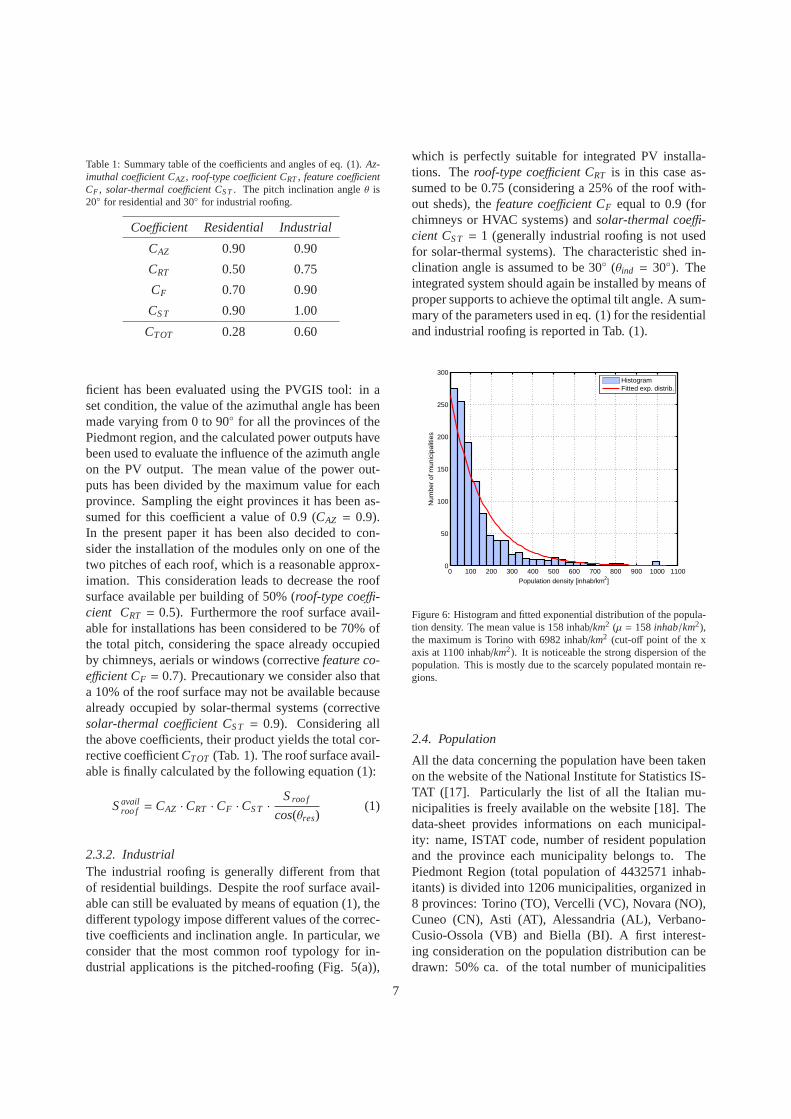
Table 1: Summary table of the coefficients and angles of eq. (1).Az-imuthal coefficient CAZ, roof-type coefficient CRT, feature coefficientCF , solar-thermal coefficient CS T. The pitch inclination angleθ is20◦ for residential and 30◦ for industrial roofing.

Coefficient Residential Industrial

CAZ 0.90 0.90

CRT 0.50 0.75

CF 0.70 0.90

CS T 0.90 1.00

CTOT 0.28 0.60

ficient has been evaluated using the PVGIS tool: in aset condition, the value of the azimuthal angle has beenmade varying from 0 to 90◦ for all the provinces of thePiedmont region, and the calculated power outputs havebeen used to evaluate the influence of the azimuth angleon the PV output. The mean value of the power out-puts has been divided by the maximum value for eachprovince. Sampling the eight provinces it has been as-sumed for this coefficient a value of 0.9 (CAZ = 0.9).In the present paper it has been also decided to con-sider the installation of the modules only on one of thetwo pitches of each roof, which is a reasonable approx-imation. This consideration leads to decrease the roofsurface available per building of 50% (roof-type coeffi-cient CRT = 0.5). Furthermore the roof surface avail-able for installations has been considered to be 70% ofthe total pitch, considering the space already occupiedby chimneys, aerials or windows (correctivefeature co-efficient CF = 0.7). Precautionary we consider also thata 10% of the roof surface may not be available becausealready occupied by solar-thermal systems (correctivesolar-thermal coefficient CS T = 0.9). Considering allthe above coefficients, their product yields the total cor-rective coefficientCTOT (Tab. 1). The roof surface avail-able is finally calculated by the following equation (1):

Savailroo f = CAZ ·CRT ·CF ·CS T ·

Sroo f

cos(θres)(1)

2.3.2. IndustrialThe industrial roofing is generally different from thatof residential buildings. Despite the roof surface avail-able can still be evaluated by means of equation (1), thedifferent typology impose different values of the correc-tive coefficients and inclination angle. In particular, weconsider that the most common roof typology for in-dustrial applications is the pitched-roofing (Fig. 5(a)),

which is perfectly suitable for integrated PV installa-tions. Theroof-type coefficient CRT is in this case as-sumed to be 0.75 (considering a 25% of the roof with-out sheds), thefeature coefficient CF equal to 0.9 (forchimneys or HVAC systems) andsolar-thermal coeffi-cient CS T = 1 (generally industrial roofing is not usedfor solar-thermal systems). The characteristic shed in-clination angle is assumed to be 30◦ (θind = 30◦). Theintegrated system should again be installed by means ofproper supports to achieve the optimal tilt angle. A sum-mary of the parameters used in eq. (1) for the residentialand industrial roofing is reported in Tab. (1).

0 100 200 300 400 500 600 700 800 900 1000 11000

50

100

150

200

250

300

Population density [inhab/km2]

Num

ber

of m

unic

ipal

ities

HistogramFitted exp. distrib.

Figure 6: Histogram and fitted exponential distribution of the popula-tion density. The mean value is 158 inhab/km2 (µ = 158 inhab/km2),the maximum is Torino with 6982 inhab/km2 (cut-off point of the xaxis at 1100 inhab/km2). It is noticeable the strong dispersion of thepopulation. This is mostly due to the scarcely populated montain re-gions.

2.4. Population

All the data concerning the population have been takenon the website of the National Institute for Statistics IS-TAT ([17]. Particularly the list of all the Italian mu-nicipalities is freely available on the website [18]. Thedata-sheet provides informations on each municipal-ity: name, ISTAT code, number of resident populationand the province each municipality belongs to. ThePiedmont Region (total population of 4432571 inhab-itants) is divided into 1206 municipalities, organized in8 provinces: Torino (TO), Vercelli (VC), Novara (NO),Cuneo (CN), Asti (AT), Alessandria (AL), Verbano-Cusio-Ossola (VB) and Biella (BI). A first interest-ing consideration on the population distribution can bedrawn: 50% ca. of the total number of municipalities

7

counts less than 1000 inhabitants. The municipalitieswith more than 50000 inhabitants are only 8, and 1over 150000 (Torino, with 910000 inhabitants ca.). Themean population density is 158 inhabitants perkm2, themaximux belongs to Torino, with 6982 inhabitants perkm2. It is noticeable that the Piedmont region is char-acterized by a very high concentration of the populationin the main cities (Torino by far over the others). Theregion presents a strong dispersion of population out-side the main cities. This disparity is mostly due to ahigh number of municipalities located in the mountainregion of the Alps which are scarcely populated. Fig.6 show the histogram and fitted exponential distributionof the population density over the region. For the sakeof clarity, we briefly remind the definition of the pdf(probability density function) of an exponential distri-bution for a sample x (eq. 2):

f (x | µ) =1µ· e−

xµ (2)

2.5. Energy conversion

At today, the most employed PV module technolo-gies are essentially three:mono-crystalline (single-crystalline), poly-crystalline (multi-crystalline)siliconandthin film (amorphous silicon). The mono-crystallinesilicon is the oldest and more expensive productiontechnique, but it is actually the most efficient sunlightconversion technology available. The poly-crystallinehas a slightly lower conversion efficiency compared tothe mono-crystalline, but the manifacturing costs arealso lower. The thin film is obtained by vaporizationand deposition of the silicon on glass or stainless steel.The production cost of this last technology is lowerthan any other method, but the conversion efficiency isalso low. Generally the PV module manifacturers pro-vide thenominal peak powerat Standard Test Condi-tions (STC), which means at 1000W/m2 solar irradi-ance (H = 1000W/m2), a module temperature of 25◦C(Tmod = 25◦C) and with an air mass 1.5 (AM1.5)2 spec-trum. At today, the PV module market is extremely dy-namic, there is a wide range of technologies (continu-ously changing) and a multiplicity of declared efficien-cies by manifacturers for the various module typologies.For the purpose of the present study, it has been decidedto assume the following representative values: mono-crystallineηMC = 15%, poly-crystallineηPC = 12% andthin film ηT F = 6%. It is well known that the efficiency

2The air mass coefficient characterizes the solar spectrum after thesolar radiation has traveled through the atmosphere.

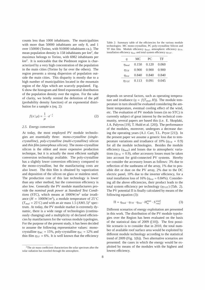
Table 2: Summary table of the efficiencies for the various moduletechnologies: MC mono-crystalline, PC poly-crystalline Silicon andTF thin film. Module efficiency ηmod, atmospheric efficiency ηT H,installation efficiencyηinst and total system efficiencyηTOT.

η MC PC TF

ηmod 0.150 0.120 0.060

ηT H 0.900 0.900 0.900

ηinst 0.840 0.840 0.840

ηTOT 0.113 0.091 0.045

depends on several factors, such as operating tempera-ture and irradiance (η = f (Tmod,H)). The module tem-perature in turn should be evaluated considering the am-bient temperature, eventual cooling effect of the wind,etc. The evaluation of PV module losses (in no STC) iscurrently subject of great interest by the technical com-munity, several papers are based this (i.e. E. Skoplaki,J.A. Palyvos [19], T. Huld et al. [20]). The performanceof the modules, moreover, undergoes a decrease dur-ing the operating years (A.J. Carr, T.L. Pryor [21]). Inthe present paper we assume a generic loss due to tem-perature variations and irradiance of 10% (ηT H = 0.9)for all the module technologies. Besides the moduleefficiency (ηmod) and losses due to atmospheric varia-tions (ηT H = 0.9), other accessory losses must be takeninto account for grid-connected PV systems. Herebywe consider the accessory losses as follows: 3% due toreflection of the sunbeams of the array, 1% due to pos-sible dirt or dust on the PV array, 2% due to the DCelectric panel, 10% due to the inverter efficiency, for atotal installation loss of 16% (ηinst = 0.84%). Consider-ing all the above efficiencies, their product leads to thetotal system efficiency per technology (ηTOT) (Tab. 2).The PV potentialΠ is finally calculated by means of thefollowing equation (3):

Π = ηmod · ηT H · ηinst · Hmunm · Savail

roo f (3)

Different scenarios of energy exploitation are presentedin this work. The distribution of the PV module typolo-gies over the Region has been evaluated on the basisof the statistical data of 2009 ([10]). The first possi-ble scenario is to consider that in 2010, the total num-ber of available roof surface area would be exploited bydifferent module technology according to the statisticaltrend of 2009 (Fig. 1(b)). Two alternative scenarios arepresented: the cases in which the energy would be ex-ploited by means of the modules with the highest andlowest efficiency.

8

AL AT BI CN NO TO VB VC0

2000

4000

6000

8000

10000

12000

Province

Net

ele

ctric

al e

nerg

y co

nsum

ptio

n [G

Wh]

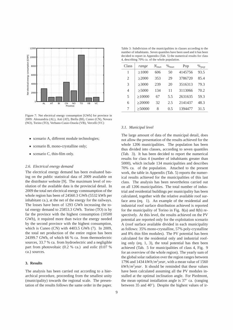
Figure 7: Net electrical energy consumption [GWh] for province in2009: Alessandria (AL), Asti (AT), Biella (BI), Cuneo (CN),Novara(NO), Torino (TO), Verbano-Cusio-Ossola (VB), Vercelli (VC)

• scenario A, different module technologies;

• scenario B, mono-crystalline only;

• scenario C, thin-film only.

2.6. Electrical energy demand

The electrical energy demand has been evaluated bas-ing on the public statistical data of 2009 available onthe distributor website [9]. The maximum level of res-olution of the available data is the provincial detail. In2009 the total net electrical energy comnsumption of thewhole region has been of 24560.3 GWh (5532 kWh perinhabitant ca.), at the net of the energy for the railways.The losses have been of 1293 GWh increasing the to-tal energy demand to 25853.3 GWh. Torino (TO) is byfar the province with the highest consumption (10500GWh), it required more than twice the energy neededby the second province with the highest consumption,which is Cuneo (CN) with 4403.5 GWh (7). In 2009,the total net production of the entire region has been24399.7 GWh, of which 66 % ca. from thermoelectricsources, 33.7 % ca. from hydroelectric and a negligiblepart from photovoltaic (0.2 % ca.) and eolic (0.07 %ca.) sources.

3. Results

The analysis has been carried out according to a hier-archical procedure, proceeding from the smallest unity(municipality) towards the regional scale. The presen-tation of the results follows the same order in the paper.

Table 3: Subdivision of the municipalities in classes according to thenumber of inhabitants. Seven quantiles have been used and it has beendecided to report in Appendix (Tab. 5) the numerical results for class4, describing 70% ca. of the whole population.

Class range Nmun %mun Pop %pop

1 ≥1000 606 50 4145756 93.5

2 ≥2000 353 29 3786720 85.4

3 ≥3000 239 20 3516313 79.3

4 ≥5000 134 11 3113066 70.2

5 ≥10000 67 5.5 2631635 59.3

6 ≥20000 32 2.5 2141437 48.3

7 ≥50000 8 0.5 1394477 31.5

3.1. Municipal level

The large amount of data of the municipal detail, doesnot allow the presentation of the results achieved for thewhole 1206 municipalities. The population has beenthus divided into classes, according to seven quantiles(Tab. 3). It has been decided to report the numericalresults for class 4 (number of inhabitants greater than5000), which include 134 municipalities and describes70% ca. of the population. Attached to the presentwork, the table in Appendix (Tab. 5) reports the numer-ical results achieved for the municipalities of this lastclass. The analysis has been nevertheless carried outon all 1206 municipalities. The total number of indus-trial and residential buildings per municipality has beencalculated, together with the relative available roof sur-face area (eq. 1). An example of the residential andindustrial roof surface distribution achieved is reportedfor the municipality of Torino in Fig. 8(a) and 8(b) re-spectively. At this level, the results achieved on the PVpotential are reported only for the exploitation scenarioA (roof surface available divided in each municipalityas follows: 35% mono-crystalline, 57% poly-crystallineand 8% thin film modules). The PV potential has beencalculated for the residential only and industrial roof-ing only (eq. 1, 3), the total potential has then beenachieved (Tab. 5 for municipalities of class 4, Fig. 9for an overview of the whole region). The yearly sum ofthe global solar radiation over the region ranges between1796 and 1434kWh/m2year, with a mean value of 1560kWh/m2year. It should be reminded that these valueshave been calculated assuming all the PV modules in-stalled at the optimal inclination angle. For Piedmont,the mean optimal installation angle is 37◦ ca. (rangingbetween 35 and 40◦). Despite the highest values of ir-

9

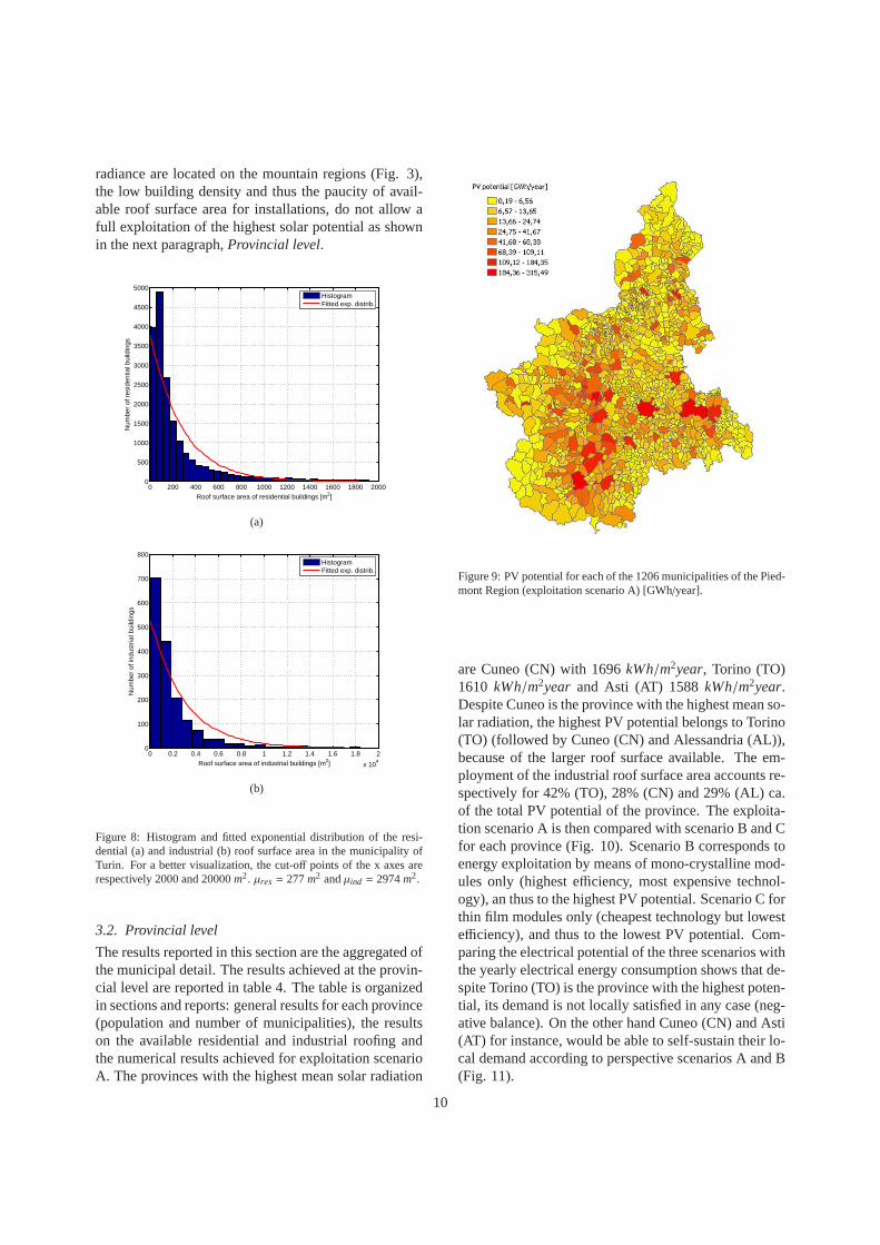
radiance are located on the mountain regions (Fig. 3),the low building density and thus the paucity of avail-able roof surface area for installations, do not allow afull exploitation of the highest solar potential as shownin the next paragraph,Provincial level.

0 200 400 600 800 1000 1200 1400 1600 1800 20000

500

1000

1500

2000

2500

3000

3500

4000

4500

5000

Roof surface area of residential buildings [m2]

Num

ber

of r

esid

entia

l bui

ldin

gs

HistogramFitted exp. distrib.

(a)

0 0.2 0.4 0.6 0.8 1 1.2 1.4 1.6 1.8 2

x 104

0

100

200

300

400

500

600

700

800

Roof surface area of industrial buildings [m2]

Num

ber

of in

dust

rial b

uild

ings

HistogramFitted exp. distrib.

(b)

Figure 8: Histogram and fitted exponential distribution of the resi-dential (a) and industrial (b) roof surface area in the municipality ofTurin. For a better visualization, the cut-off points of the x axes arerespectively 2000 and 20000m2. µres = 277m2 andµind = 2974m2.

3.2. Provincial level

The results reported in this section are the aggregated ofthe municipal detail. The results achieved at the provin-cial level are reported in table 4. The table is organizedin sections and reports: general results for each province(population and number of municipalities), the resultson the available residential and industrial roofing andthe numerical results achieved for exploitation scenarioA. The provinces with the highest mean solar radiation

Figure 9: PV potential for each of the 1206 municipalities of the Pied-mont Region (exploitation scenario A) [GWh/year].

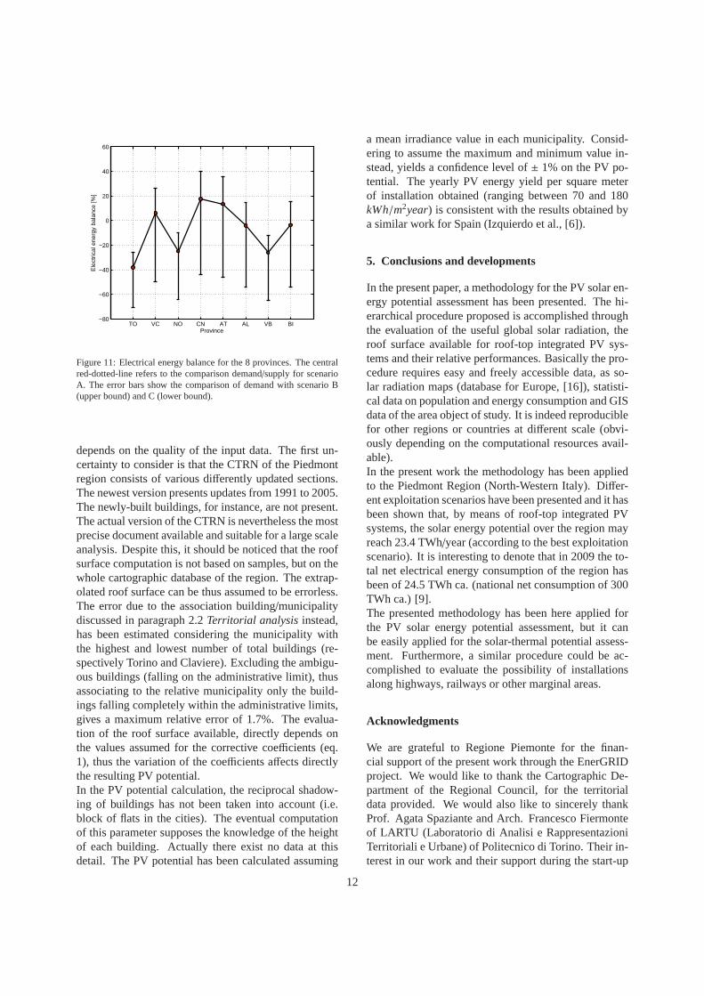
are Cuneo (CN) with 1696kWh/m2year, Torino (TO)1610 kWh/m2year and Asti (AT) 1588kWh/m2year.Despite Cuneo is the province with the highest mean so-lar radiation, the highest PV potential belongs to Torino(TO) (followed by Cuneo (CN) and Alessandria (AL)),because of the larger roof surface available. The em-ployment of the industrial roof surface area accounts re-spectively for 42% (TO), 28% (CN) and 29% (AL) ca.of the total PV potential of the province. The exploita-tion scenario A is then compared with scenario B and Cfor each province (Fig. 10). Scenario B corresponds toenergy exploitation by means of mono-crystalline mod-ules only (highest efficiency, most expensive technol-ogy), an thus to the highest PV potential. Scenario C forthin film modules only (cheapest technology but lowestefficiency), and thus to the lowest PV potential. Com-paring the electrical potential of the three scenarios withthe yearly electrical energy consumption shows that de-spite Torino (TO) is the province with the highest poten-tial, its demand is not locally satisfied in any case (neg-ative balance). On the other hand Cuneo (CN) and Asti(AT) for instance, would be able to self-sustain their lo-cal demand according to perspective scenarios A and B(Fig. 11).

10

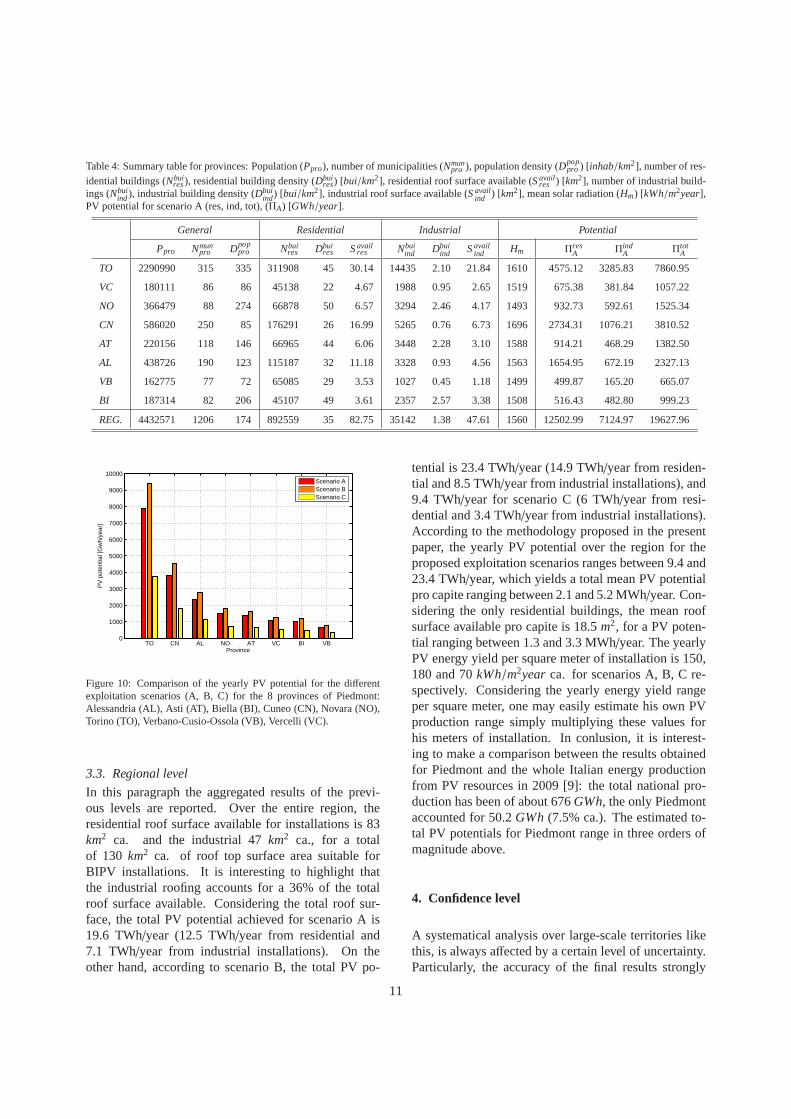
Table 4: Summary table for provinces: Population (Ppro), number of municipalities (Nmunpro ), population density (Dpop

pro ) [inhab/km2], number of res-

idential buildings (Nbuires), residential building density (Dbui

res) [bui/km2], residential roof surface available (Savailres ) [km2], number of industrial build-

ings (Nbuiind), industrial building density (Dbui

ind) [bui/km2], industrial roof surface available (Savailind ) [km2], mean solar radiation (Hm) [kWh/m2year],

PV potential for scenario A (res, ind, tot), (ΠA) [GWh/year].

General Residential Industrial Potential

Ppro Nmunpro Dpop

pro Nbuires Dbui

res Savailres Nbui

ind Dbuiind Savail

ind Hm ΠresA Πind

A ΠtotA

TO 2290990 315 335 311908 45 30.14 14435 2.10 21.84 1610 4575.12 3285.83 7860.95

VC 180111 86 86 45138 22 4.67 1988 0.95 2.65 1519 675.38 381.84 1057.22

NO 366479 88 274 66878 50 6.57 3294 2.46 4.17 1493 932.73 592.61 1525.34

CN 586020 250 85 176291 26 16.99 5265 0.76 6.73 1696 2734.31 1076.21 3810.52

AT 220156 118 146 66965 44 6.06 3448 2.28 3.10 1588 914.21 468.29 1382.50

AL 438726 190 123 115187 32 11.18 3328 0.93 4.56 1563 1654.95 672.19 2327.13

VB 162775 77 72 65085 29 3.53 1027 0.45 1.18 1499 499.87 165.20 665.07

BI 187314 82 206 45107 49 3.61 2357 2.57 3.38 1508 516.43 482.80 999.23

REG. 4432571 1206 174 892559 35 82.75 35142 1.38 47.61 1560 12502.99 7124.97 19627.96

TO CN AL NO AT VC BI VB0

1000

2000

3000

4000

5000

6000

7000

8000

9000

10000

Province

PV

pot

entia

l [G

wh/

year

]

Scenario AScenario BScenario C

Figure 10: Comparison of the yearly PV potential for the differentexploitation scenarios (A, B, C) for the 8 provinces of Piedmont:Alessandria (AL), Asti (AT), Biella (BI), Cuneo (CN), Novara (NO),Torino (TO), Verbano-Cusio-Ossola (VB), Vercelli (VC).

3.3. Regional level

In this paragraph the aggregated results of the previ-ous levels are reported. Over the entire region, theresidential roof surface available for installations is 83km2 ca. and the industrial 47km2 ca., for a totalof 130 km2 ca. of roof top surface area suitable forBIPV installations. It is interesting to highlight thatthe industrial roofing accounts for a 36% of the totalroof surface available. Considering the total roof sur-face, the total PV potential achieved for scenario A is19.6 TWh/year (12.5 TWh/year from residential and7.1 TWh/year from industrial installations). On theother hand, according to scenario B, the total PV po-

tential is 23.4 TWh/year (14.9 TWh/year from residen-tial and 8.5 TWh/year from industrial installations), and9.4 TWh/year for scenario C (6 TWh/year from resi-dential and 3.4 TWh/year from industrial installations).According to the methodology proposed in the presentpaper, the yearly PV potential over the region for theproposed exploitation scenarios ranges between 9.4 and23.4 TWh/year, which yields a total mean PV potentialpro capite ranging between 2.1 and 5.2 MWh/year. Con-sidering the only residential buildings, the mean roofsurface available pro capite is 18.5m2, for a PV poten-tial ranging between 1.3 and 3.3 MWh/year. The yearlyPV energy yield per square meter of installation is 150,180 and 70kWh/m2year ca. for scenarios A, B, C re-spectively. Considering the yearly energy yield rangeper square meter, one may easily estimate his own PVproduction range simply multiplying these values forhis meters of installation. In conlusion, it is interest-ing to make a comparison between the results obtainedfor Piedmont and the whole Italian energy productionfrom PV resources in 2009 [9]: the total national pro-duction has been of about 676GWh, the only Piedmontaccounted for 50.2GWh(7.5% ca.). The estimated to-tal PV potentials for Piedmont range in three orders ofmagnitude above.

4. Confidence level

A systematical analysis over large-scale territories likethis, is always affected by a certain level of uncertainty.Particularly, the accuracy of the final results strongly

11

TO VC NO CN AT AL VB BI−80

−60

−40

−20

0

20

40

60

Province

Ele

ctric

al e

nerg

y ba

lanc

e [%

]

Figure 11: Electrical energy balance for the 8 provinces. The centralred-dotted-line refers to the comparison demand/supply for scenarioA. The error bars show the comparison of demand with scenario B(upper bound) and C (lower bound).

depends on the quality of the input data. The first un-certainty to consider is that the CTRN of the Piedmontregion consists of various differently updated sections.The newest version presents updates from 1991 to 2005.The newly-built buildings, for instance, are not present.The actual version of the CTRN is nevertheless the mostprecise document available and suitable for a large scaleanalysis. Despite this, it should be noticed that the roofsurface computation is not based on samples, but on thewhole cartographic database of the region. The extrap-olated roof surface can be thus assumed to be errorless.The error due to the association building/municipalitydiscussed in paragraph 2.2Territorial analysisinstead,has been estimated considering the municipality withthe highest and lowest number of total buildings (re-spectively Torino and Claviere). Excluding the ambigu-ous buildings (falling on the administrative limit), thusassociating to the relative municipality only the build-ings falling completely within the administrative limits,gives a maximum relative error of 1.7%. The evalua-tion of the roof surface available, directly depends onthe values assumed for the corrective coefficients (eq.1), thus the variation of the coefficients affects directlythe resulting PV potential.In the PV potential calculation, the reciprocal shadow-ing of buildings has not been taken into account (i.e.block of flats in the cities). The eventual computationof this parameter supposes the knowledge of the heightof each building. Actually there exist no data at thisdetail. The PV potential has been calculated assuming

a mean irradiance value in each municipality. Consid-ering to assume the maximum and minimum value in-stead, yields a confidence level of± 1% on the PV po-tential. The yearly PV energy yield per square meterof installation obtained (ranging between 70 and 180kWh/m2year) is consistent with the results obtained bya similar work for Spain (Izquierdo et al., [6]).

5. Conclusions and developments

In the present paper, a methodology for the PV solar en-ergy potential assessment has been presented. The hi-erarchical procedure proposed is accomplished throughthe evaluation of the useful global solar radiation, theroof surface available for roof-top integrated PV sys-tems and their relative performances. Basically the pro-cedure requires easy and freely accessible data, as so-lar radiation maps (database for Europe, [16]), statisti-cal data on population and energy consumption and GISdata of the area object of study. It is indeed reproduciblefor other regions or countries at different scale (obvi-ously depending on the computational resources avail-able).In the present work the methodology has been appliedto the Piedmont Region (North-Western Italy). Differ-ent exploitation scenarios have been presented and it hasbeen shown that, by means of roof-top integrated PVsystems, the solar energy potential over the region mayreach 23.4 TWh/year (according to the best exploitationscenario). It is interesting to denote that in 2009 the to-tal net electrical energy consumption of the region hasbeen of 24.5 TWh ca. (national net consumption of 300TWh ca.) [9].The presented methodology has been here applied forthe PV solar energy potential assessment, but it canbe easily applied for the solar-thermal potential assess-ment. Furthermore, a similar procedure could be ac-complished to evaluate the possibility of installationsalong highways, railways or other marginal areas.

Acknowledgments

We are grateful to Regione Piemonte for the finan-cial support of the present work through the EnerGRIDproject. We would like to thank the Cartographic De-partment of the Regional Council, for the territorialdata provided. We would also like to sincerely thankProf. Agata Spaziante and Arch. Francesco Fiermonteof LARTU (Laboratorio di Analisi e RappresentazioniTerritoriali e Urbane) of Politecnico di Torino. Their in-terest in our work and their support during the start-up

12

phase of the territorial analysis has been really appre-ciated. Thanks to Thomas Huld, of the Joint ResearchCentre of the European Commission, for his hints on thesolar radiation data. We are also thankful to our friendSalvador Izquierdo, who first applied a similar method-ology to Spain ([6]), for our enlightening discussionsand comparisons.

References[1] Conto Energia 2010. GSE S.p.a., Gestore Servizi Energetici.

Publicly-owned company promoting and supporting renewableenergy sources (RES) in Italy. 2010, (www.gse.it).

[2] Regional Council of Piedmont. 2010,(www.regione.piemonte.it).

[3] Castro, M., Delgado, A., Argul, F., Colmenar, A., Yeves, F.,Peire, J.,Grid-connected PV buildings: analysis of future sce-narios with an example of southern Spain, Solar Energy 79(2005) 8695.

[4] Sorensen, B.,GIS management of solar resource data, Solar En-ergy Materials and Solar Cells, 67 (2001)(14), 503509.

[5] EEA, 2010. European Environment Agency(http://www.eea.europa.eu/data-and-maps/).

[6] Izquierdo S, Rodrigues M, Fueyo N.,A method for estimatingthe geographical distribution of the available roof surface areafor large-scale photovoltaic energy-potential evaluations, SolarEnergy 82 (2008) 92939.

[7] Kabir, Md.H., Endlicher, W., Jgermeyr, J.,Calculation ofbright roof-tops for solar PV applications in Dhaka Megacity,Bangladesh, Renewable Energy 35 (8) (2010), pp. 1760-1764.

[8] Wiginton, L.K., Nguyen, H.T., Pearce, J.M.,Quantifyingrooftop solar photovoltaic potential for regional renewable en-ergy policy, Computers, Environment and Urban Systems 34 (4)(2010), pp. 345-357.

[9] Terna S.p.a., 2010. Energy Transmission Grid Operator.Statis-tical Data on electricity in Italy (for 2009), (www.terna.it).

[10] GSE S.p.a., 2010. Gestore Servizi Energetici. Publicly-ownedcompany promoting and supporting renewable energy sources(RES) in Italy.Statistical Data on photovoltaic solar energy inItaly for 2009, (www.gse.it).

[11] MarcelSuri, Thomas Huld, Tomas Cebecauer, Ewan D. Dunlop,Geographic Aspects of Photovoltaics in Europe: Contribution ofthe PVGIS Website, IEEE Journal of Selected Topics in AppliedEarth Observations and Remote Sensing, v 1, n 1, p 34-41, 2008.

[12] Suri M., Hofierka J.,A new GIS-based solar radiation modeland its application to photovoltaic assessments, Transactions inGIS 8, 175190, 2004.

[13] Suri M., Dunlop E. D., Huld T. A., 2005.PV-GIS: A web basedsolar radiation database for the calculation of PV potentialin Europe, International Journal of Sustainable Energy 24 (2),5567.

[14] MarcelSuri, Thomas Huld, Tomas Cebecauer, Ewan D. Dunlop,Heinz A. Ossenbrink,Potential of solar electricity generationin the European Union member states and candidate countries,Solar Energy 81 (2007) 12951305.

[15] ESRA, 2010. European Solar Radiation Atlas(http://www.helioclim.org/esra/).

[16] JRC, 2010. Joint Research Centre of the Euro-pean Commission, IE Institute for Energy.PVGIS,(http://re.jrc.ec.europa.eu/pvgis/).

[17] ISTAT 2010. National Institute for Statistics, (www.istat.it).[18] ISTAT 2010. National Institute for Statistics,

(www.istat.it/strumenti/definizioni/comuni/).[19] E. Skoplaki, J.A. Palyvos,On the temperature dependence of

photovoltaic module electrical performance: A review of effi-

ciency/power correlations, Solar Energy 83 (2009) 614624.[20] Thomas Huld, Ralph Gottschalg, Hans Georg Beyer, Marko

Topic,Mapping the performance of PV modules, effects of mod-ule type and data averaging, Solar Energy 84 (2010) 324338.

[21] A.J. Carr, T.L. Pryor,A comparison of the performance of dif-ferent PV module types in temperate climates, Solar Energy 76(2004) 285294.

13

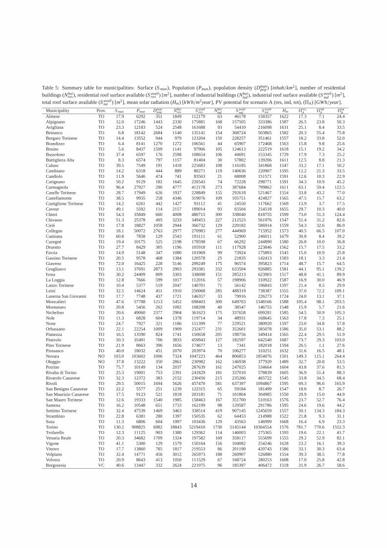
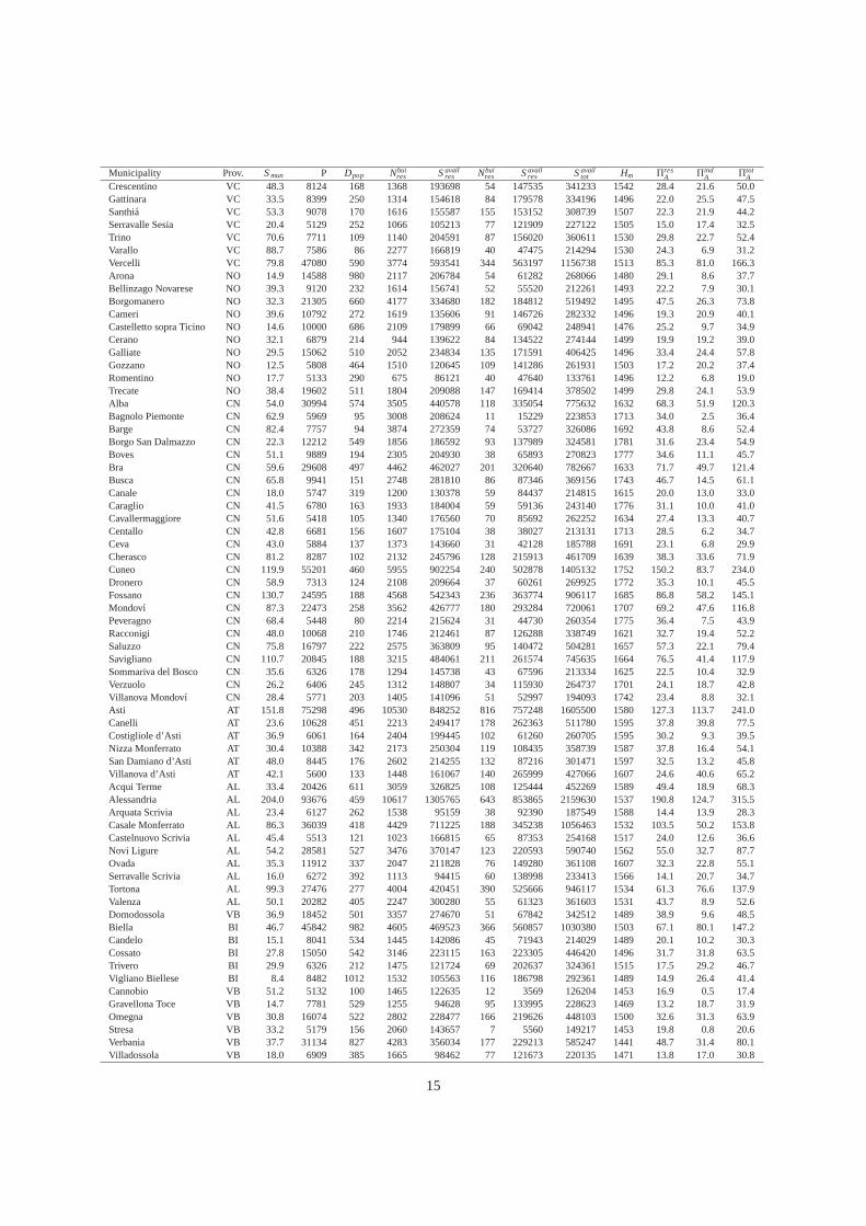
Table 5: Summary table for municipalities: Surface (Smun), Population (Pmun), population density (Dmunpop) [inhab/km2], number of residential

buildings (Nbuires), residential roof surface available (Savail

res ) [m2], number of industrial buildings (Nbuiind), industrial roof surface available (Savail

ind ) [m2],total roof surface available (Savail

tot ) [m2], mean solar radiation (Hm) [kWh/m2year], PV potential for scenario A (res, ind, tot), (ΠA) [GWh/year].

Municipality Prov. Smun Pmun Dmunpop Nbui

res Savailres Nbui

ind Savailind Savail

tot Hm ΠresA Πind

A ΠtotA

Almese TO 17.9 6292 351 1849 112179 63 46178 158357 1622 17.3 7.1 24.4Alpignano TO 12.0 17246 1443 2330 175881 168 157505 333386 1587 26.5 23.8 50.3Avigliana TO 23.3 12183 524 2548 161688 93 54410 216098 1631 25.1 8.4 33.5Beinasco TO 6.8 18142 2684 1140 135141 154 368724 503865 1582 20.3 55.4 75.8Borgaro Torinese TO 14.4 13552 944 979 123204 150 228257 351461 1557 18.2 33.8 52.0Brandizzo TO 6.4 8141 1270 1272 106561 44 65907 172468 1563 15.8 9.8 25.6Bruino TO 5.6 8437 1509 1141 97906 105 124613 222519 1618 15.1 19.2 34.2Bussoleno TO 37.4 6597 176 2598 108654 106 44691 153345 1729 17.9 7.3 25.2Buttigliera Alta TO 8.3 6574 797 1157 81404 30 57802 139206 161112.5 8.8 21.3Caluso TO 39.5 7549 191 1418 225683 108 116185 341868 1547 33.217.1 50.2Cambiano TO 14.2 6318 444 889 80271 119 140636 220907 1595 12.2 21.3 33.5Candiolo TO 11.9 5646 474 741 83563 21 68008 151571 1591 12.6 10.3 22.9Carignano TO 50.2 9129 182 1645 226543 74 72228 298771 1591 34.3 10.9 45.2Carmagnola TO 96.4 27927 290 4777 412178 273 387684 799862 1611 63.1 59.4 122.5Caselle Torinese TO 28.7 17949 626 1937 228849 155 292618 521467 1554 33.8 43.2 77.0Castellamonte TO 38.5 9935 258 4346 319076 109 105751 424827 1565 47.5 15.7 63.2Castiglione Torinese TO 14.2 6261 442 1427 93112 41 24550 1176621569 13.9 3.7 17.5Cavour TO 49.1 5592 114 2157 189014 93 65504 254518 1655 29.7 10.3 40.0Chieri TO 54.3 35849 660 4008 480715 300 338040 818755 1599 73.051.3 124.4Chivasso TO 51.3 25378 495 3233 349453 227 212523 561976 1547 51.4 31.2 82.6Cirie TO 17.8 18827 1058 2944 366732 129 220182 586914 1559 54.3 32.6 86.9Collegno TO 18.1 50072 2763 2977 270983 277 444969 715952 1573 40.5 66.5 107.0Cumiana TO 60.8 7858 129 2543 193111 61 52900 246011 1679 30.8 8.4 39.2Cuorgne TO 19.4 10175 525 2198 178598 67 66292 244890 1580 26.8 10.0 36.8Druento TO 27.7 8429 305 1196 105918 111 117928 223846 1562 15.717.5 33.2Favria TO 14.9 5148 347 1080 101969 99 73924 175893 1545 15.0 10.9 25.8Gassino Torinese TO 20.5 9578 468 1384 120578 25 21835 142413 1583 18.1 3.3 21.4Giaveno TO 72.0 16425 228 5146 299249 175 96574 395823 1714 48.7 15.7 64.5Grugliasco TO 13.1 37691 2873 2903 293381 332 633504 926885 158144.1 95.1 139.2Ivrea TO 30.2 24409 809 3303 338690 151 285213 623903 1517 48.8 41.1 89.9La Loggia TO 12.8 7666 599 1017 112016 57 198906 310922 1587 16.9 30.0 46.9Lanzo Torinese TO 10.4 5377 519 2047 140701 71 56142 196843 1597 21.4 8.5 29.9Leinı TO 32.5 14624 451 1910 250068 285 488319 738387 1555 37.0 72.2 109.1Luserna San Giovanni TO 17.7 7748 437 1721 146357 33 79916 226273 1724 24.0 13.1 37.1Moncalieri TO 47.6 57788 1213 5452 698403 300 649763 1348166 1588105.4 98.1 203.5Montanaro TO 20.8 5456 262 1092 108208 40 38547 146755 1548 15.9 5.7 21.6Nichelino TO 20.6 49060 2377 2904 361623 175 337658 699281 158554.5 50.9 105.3Nole TO 11.3 6828 604 1378 119714 34 48931 168645 1563 17.8 7.325.1None TO 24.7 7927 321 1186 151399 77 229521 380920 1597 23.0 34.8 57.8Orbassano TO 22.1 22254 1009 1909 232477 231 352601 585078 1586 35.0 53.1 88.2Pianezza TO 16.5 13590 824 1741 150658 205 198756 349414 1565 22.429.5 51.9Pinerolo TO 50.3 35491 706 3833 459943 127 182597 642540 1687 73.7 29.3 103.0Pino Torinese TO 21.9 8663 396 1656 174677 13 7341 182018 1594 26.5 1.1 27.6Piossasco TO 40.0 18032 451 2070 203974 70 106277 310251 1632 31.6 16.5 48.1Novara NO 103.0 103602 1006 7324 1047223 464 806853 1854076 1501 149.3 115.1 264.4Oleggio NO 37.8 13222 350 2861 230982 162 146938 377920 1489 32.7 20.8 53.5Poirino TO 75.7 10149 134 2037 287639 161 247025 534664 1604 43.8 37.6 81.5Rivalta di Torino TO 25.3 19001 753 2391 241829 181 337010 578839 1605 36.9 51.4 88.3Rivarolo Canavese TO 32.3 12372 383 2152 230456 215 235266 4657221545 33.8 34.5 68.4Rivoli TO 29.5 50015 1694 5626 457470 581 637397 1094867 159569.3 96.6 165.9San Benigno Canavese TO 22.2 5577 251 1239 122315 65 59184 181499 1547 18.0 8.7 26.7San Maurizio Canavese TO 17.5 9123 521 1818 203181 71 101804 304985 1550 29.9 15.0 44.9San Mauro Torinese TO 12.6 19333 1540 1985 158463 167 351700 5101631576 23.7 52.7 76.4Santena TO 16.2 10548 651 1733 162199 98 129587 291786 1595 24.619.6 44.2Settimo Torinese TO 32.4 47539 1469 3463 338514 419 907145 1245659 1557 50.1 134.3 184.3Strambino TO 22.8 6381 280 1397 150535 62 64453 214988 1522 21.89.3 31.1Susa TO 11.3 6806 604 1997 103436 129 43563 146999 1668 16.4 6.9 23.3Torino TO 130.2 908825 6982 18843 5219410 1730 5145144 10364554 1576 781.7 770.6 1552.3Trofarello TO 12.3 11125 903 1380 129362 114 146003 275365 1593 19.6 22.1 41.7Venaria Reale TO 20.3 34682 1709 1324 197582 169 358117 555699 155529.2 52.9 82.1Vigone TO 41.1 5300 129 1579 150164 156 104082 254246 1628 23.2 16.1 39.3Vinovo TO 17.7 13860 785 1817 219553 86 201190 420743 1586 33.1 30.3 63.4Volpiano TO 32.4 14771 456 3012 265973 188 260907 526880 1554 39.3 38.5 77.8Volvera TO 20.9 8643 413 1050 111529 67 168724 280253 1608 17.0 25.8 42.8Borgosesia VC 40.6 13447 332 2624 221075 96 185397 406472 151831.9 26.7 58.6

14

Municipality Prov. Smun P Dpop Nbuires Savail

res Nbuires Savail

res Savailtot Hm Πres

A ΠindA Πtot

ACrescentino VC 48.3 8124 168 1368 193698 54 147535 341233 1542 28.4 21.6 50.0Gattinara VC 33.5 8399 250 1314 154618 84 179578 334196 1496 22.025.5 47.5Santhia VC 53.3 9078 170 1616 155587 155 153152 308739 1507 22.3 21.944.2Serravalle Sesia VC 20.4 5129 252 1066 105213 77 121909 227122 150515.0 17.4 32.5Trino VC 70.6 7711 109 1140 204591 87 156020 360611 1530 29.8 22.7 52.4Varallo VC 88.7 7586 86 2277 166819 40 47475 214294 1530 24.3 6.9 31.2Vercelli VC 79.8 47080 590 3774 593541 344 563197 1156738 1513 85.3 81.0 166.3Arona NO 14.9 14588 980 2117 206784 54 61282 268066 1480 29.1 8.6 37.7Bellinzago Novarese NO 39.3 9120 232 1614 156741 52 55520 212261 1493 22.2 7.9 30.1Borgomanero NO 32.3 21305 660 4177 334680 182 184812 519492 149547.5 26.3 73.8Cameri NO 39.6 10792 272 1619 135606 91 146726 282332 1496 19.3 20.9 40.1Castelletto sopra Ticino NO 14.6 10000 686 2109 179899 66 69042 248941 1476 25.2 9.7 34.9Cerano NO 32.1 6879 214 944 139622 84 134522 274144 1499 19.9 19.239.0Galliate NO 29.5 15062 510 2052 234834 135 171591 406425 1496 33.4 24.4 57.8Gozzano NO 12.5 5808 464 1510 120645 109 141286 261931 1503 17.2 20.2 37.4Romentino NO 17.7 5133 290 675 86121 40 47640 133761 1496 12.2 6.8 19.0Trecate NO 38.4 19602 511 1804 209088 147 169414 378502 1499 29.8 24.1 53.9Alba CN 54.0 30994 574 3505 440578 118 335054 775632 1632 68.351.9 120.3Bagnolo Piemonte CN 62.9 5969 95 3008 208624 11 15229 223853 1713 34.0 2.5 36.4Barge CN 82.4 7757 94 3874 272359 74 53727 326086 1692 43.8 8.6 52.4Borgo San Dalmazzo CN 22.3 12212 549 1856 186592 93 137989 324581 1781 31.6 23.4 54.9Boves CN 51.1 9889 194 2305 204930 38 65893 270823 1777 34.6 11.1 45.7Bra CN 59.6 29608 497 4462 462027 201 320640 782667 1633 71.7 49.7 121.4Busca CN 65.8 9941 151 2748 281810 86 87346 369156 1743 46.7 14.5 61.1Canale CN 18.0 5747 319 1200 130378 59 84437 214815 1615 20.0 13.0 33.0Caraglio CN 41.5 6780 163 1933 184004 59 59136 243140 1776 31.1 10.0 41.0Cavallermaggiore CN 51.6 5418 105 1340 176560 70 85692 262252 163427.4 13.3 40.7Centallo CN 42.8 6681 156 1607 175104 38 38027 213131 1713 28.5 6.2 34.7Ceva CN 43.0 5884 137 1373 143660 31 42128 185788 1691 23.1 6.829.9Cherasco CN 81.2 8287 102 2132 245796 128 215913 461709 1639 38.3 33.6 71.9Cuneo CN 119.9 55201 460 5955 902254 240 502878 1405132 1752 150.2 83.7 234.0Dronero CN 58.9 7313 124 2108 209664 37 60261 269925 1772 35.3 10.1 45.5Fossano CN 130.7 24595 188 4568 542343 236 363774 906117 1685 86.8 58.2 145.1Mondovı CN 87.3 22473 258 3562 426777 180 293284 720061 1707 69.2 47.6 116.8Peveragno CN 68.4 5448 80 2214 215624 31 44730 260354 1775 36.4 7.5 43.9Racconigi CN 48.0 10068 210 1746 212461 87 126288 338749 1621 32.7 19.4 52.2Saluzzo CN 75.8 16797 222 2575 363809 95 140472 504281 1657 57.3 22.1 79.4Savigliano CN 110.7 20845 188 3215 484061 211 261574 745635 1664 76.5 41.4 117.9Sommariva del Bosco CN 35.6 6326 178 1294 145738 43 67596 213334 1625 22.5 10.4 32.9Verzuolo CN 26.2 6406 245 1312 148807 34 115930 264737 1701 24.1 18.7 42.8Villanova Mondovı CN 28.4 5771 203 1405 141096 51 52997 194093 1742 23.4 8.8 32.1Asti AT 151.8 75298 496 10530 848252 816 757248 1605500 1580 127.3 113.7 241.0Canelli AT 23.6 10628 451 2213 249417 178 262363 511780 1595 37.8 39.8 77.5Costigliole d’Asti AT 36.9 6061 164 2404 199445 102 61260 260705 1595 30.2 9.3 39.5Nizza Monferrato AT 30.4 10388 342 2173 250304 119 108435 358739 158737.8 16.4 54.1San Damiano d’Asti AT 48.0 8445 176 2602 214255 132 87216 301471 1597 32.5 13.2 45.8Villanova d’Asti AT 42.1 5600 133 1448 161067 140 265999 4270661607 24.6 40.6 65.2Acqui Terme AL 33.4 20426 611 3059 326825 108 125444 452269 1589 49.4 18.9 68.3Alessandria AL 204.0 93676 459 10617 1305765 643 853865 21596301537 190.8 124.7 315.5Arquata Scrivia AL 23.4 6127 262 1538 95159 38 92390 187549 1588 14.4 13.9 28.3Casale Monferrato AL 86.3 36039 418 4429 711225 188 345238 1056463 1532 103.5 50.2 153.8Castelnuovo Scrivia AL 45.4 5513 121 1023 166815 65 87353 254168 1517 24.0 12.6 36.6Novi Ligure AL 54.2 28581 527 3476 370147 123 220593 590740 1562 55.0 32.7 87.7Ovada AL 35.3 11912 337 2047 211828 76 149280 361108 1607 32.3 22.8 55.1Serravalle Scrivia AL 16.0 6272 392 1113 94415 60 138998 233413 156614.1 20.7 34.7Tortona AL 99.3 27476 277 4004 420451 390 525666 946117 1534 61.3 76.6 137.9Valenza AL 50.1 20282 405 2247 300280 55 61323 361603 1531 43.7 8.9 52.6Domodossola VB 36.9 18452 501 3357 274670 51 67842 342512 1489 38.9 9.6 48.5Biella BI 46.7 45842 982 4605 469523 366 560857 1030380 1503 67.1 80.1 147.2Candelo BI 15.1 8041 534 1445 142086 45 71943 214029 1489 20.1 10.2 30.3Cossato BI 27.8 15050 542 3146 223115 163 223305 446420 1496 31.7 31.8 63.5Trivero BI 29.9 6326 212 1475 121724 69 202637 324361 1515 17.5 29.2 46.7Vigliano Biellese BI 8.4 8482 1012 1532 105563 116 186798 2923611489 14.9 26.4 41.4Cannobio VB 51.2 5132 100 1465 122635 12 3569 126204 1453 16.9 0.5 17.4Gravellona Toce VB 14.7 7781 529 1255 94628 95 133995 228623 146913.2 18.7 31.9Omegna VB 30.8 16074 522 2802 228477 166 219626 448103 1500 32.6 31.3 63.9Stresa VB 33.2 5179 156 2060 143657 7 5560 149217 1453 19.8 0.8 20.6Verbania VB 37.7 31134 827 4283 356034 177 229213 585247 1441 48.7 31.4 80.1Villadossola VB 18.0 6909 385 1665 98462 77 121673 220135 147113.8 17.0 30.8

15