Numerical Modeling of Mass-Transport

in Solid-Oxide Fuel Cells: an Open Source Library

Valerio Novaresioa,1, Marıa Garcıa-Camprubıb,1, Salvador Izquierdoa,b,Pietro Asinaria,∗, Norberto Fueyob

aDipartimento di Energetica, Politecnico di Torino, Corso Duca degli Abruzzi 24, 1019,Torino, Italy

bArea de Mecanica de Fluidos-LITEC, Universidad de Zaragoza, Marıa de Luna 3,50018, Zaragoza, Spain

Abstract

The generation of direct current electricity using Solid Oxidize Fuel Cells(SOFCs) involves several interplaying transport phenomena. Their simula-tion is crucial for the design and optimization of reliable and competitiveequipment, and for the eventual market deployment of this technology. Anopen-source library for the computational modeling of mass-transport phe-nomena in SOFCs is presented in this article. It includes several multi-component mass-transport models (ie Fickian, Stefan-Maxwell and DustyGas Model), which can be applied both within porous media and in porosity-free domains, and several diffusivity models for gases. The library has beendeveloped for its use with OpenFOAMR©, a widespread open-source code forfluid and continuum mechanics. The library can be used to model any fluidflow configuration involving multi-component transport phenomena and itis validated in this paper against the analytical solution of one-dimensionaltest cases. In addition, it is applied for the simulation of a real SOFC andfurther validated using experimental data.

Keywords: Solid Oxide Fuel Cell, Multicomponent, Mass Transfer, PorousMedia, OpenFoamR©

PROGRAM SUMMARY

∗Corresponding Author: Tel: +39 011 090 4520Email address: pietro.asinari@polito.it (Pietro Asinari)

1These authors contributed equally to this work

Preprint submitted to Computer Physics Communications January 14, 2011

Manuscript Title: Numerical Modeling of Mass-Transport in Solid-Oxide Fuel

Cells: an Open Source Library

Authors: Valerio Novaresio, Marıa Garcıa-Camprubı, Salvador Izquierdo, Pietro

Asinari, Norberto Fueyo

Program Title: multiSpeciesTransportModels

Journal Reference:

Catalogue identifier:

Licensing provisions: GNU General Public License

Programming language: C++

Computer: Any x86 (the instructions reported in the paper consider only the 64

bit case for sake of simplicity)

Operating system: Generic Linux (the instructions reported in the paper consider

only the opensource Ubuntu distribution for sake of simplicity)

Keywords: Solid Oxide Fuel Cell, Multicomponent, Mass Transfer, Porous Media,

OpenFoam R©

Classification: 12

External routines/libraries: OpenFOAMR© (version 1.6-ext) (http://www.extend-

project.de)

Nature of problem:

This software aims to simulate a steady state mass and momentum transport of

multispecies gas mixtures, eventually in porous media. In particular, the software

allows one to investigate the gas distribution in solid oxide fuel cells (SOFC) and

to predict actual performance by the polarization curve.

Solution method:

Standard finite volume method (FVM) is used for solving all the conservation

equations. The pressure-velocity coupling is solved using the SIMPLE algorithm

(eventually adding a porous drag term if required). The mass transport is calcu-

lated using different models, namely Fick, Maxwell-Stefan or dusty gas model. The

code adopts a segregated method to solve the resulting linear system of equations.

A segregated approach is also used to uncouple different regions of the SOFC,

namely gas channels, electrodes and electrolyte.

Restrictions:

When mass fluxes of the species due to Neumann and Robin boundary conditions

are too large, negative values of molar and/or mass fractions could appear and the

numerical results obtained by the library are no more reliable.

Running time:

From seconds to hours depending on the mesh size and number of species. For

example, on a 64 bit machine with Intel Core Duo T8300 and 3 GBytes of RAM,

2

the provided test run (see next) requires less than 1 second.

Contents

1 Introduction 5

2 Theoretical background: SOFC mass-transport modeling 7

2.1 Momentum-conservation equation . . . . . . . . . . . . . . . . 82.2 Mass-conservation equation . . . . . . . . . . . . . . . . . . . 82.3 Chemical-species equation . . . . . . . . . . . . . . . . . . . . 92.4 Diffusion-flux modeling . . . . . . . . . . . . . . . . . . . . . . 9

2.4.1 Fick’s model . . . . . . . . . . . . . . . . . . . . . . . . 102.4.2 Stefan-Maxwell model . . . . . . . . . . . . . . . . . . 122.4.3 Dusty gas model . . . . . . . . . . . . . . . . . . . . . 16

2.5 Diffusion-coefficient modeling . . . . . . . . . . . . . . . . . . 172.5.1 Champan-Enskog model . . . . . . . . . . . . . . . . . 172.5.2 Wilke-Lee model . . . . . . . . . . . . . . . . . . . . . 192.5.3 Fuller-Schettler-Giddings model . . . . . . . . . . . . . 192.5.4 Knudsen model . . . . . . . . . . . . . . . . . . . . . . 20

3 Overview of the software structure 20

4 Description of the individual software components 21

4.1 Multispecies mass-transfer library . . . . . . . . . . . . . . . . 214.1.1 Thermophysical models . . . . . . . . . . . . . . . . . . 214.1.2 Momentum-continuity models . . . . . . . . . . . . . . 224.1.3 Mass-transfer models . . . . . . . . . . . . . . . . . . . 224.1.4 Diffusion-coefficient models . . . . . . . . . . . . . . . 24

4.2 SOFC solver . . . . . . . . . . . . . . . . . . . . . . . . . . . . 24

5 Validation and Results 26

5.1 Validation of the multi-species mass-transfer library . . . . . . 265.1.1 Validation of Fick . . . . . . . . . . . . . . . . . . . . 265.1.2 Validation of MaxwellStefan . . . . . . . . . . . . . . 275.1.3 Validation of dustyGas . . . . . . . . . . . . . . . . . . 28

5.2 SOFC solver results and validation . . . . . . . . . . . . . . . 29

3

6 Practical issues 30

6.1 Installation instructions . . . . . . . . . . . . . . . . . . . . . 306.2 Test run description . . . . . . . . . . . . . . . . . . . . . . . 32

7 Conclusions 33

Acknowledgements 33

Nomenclature 34

References 38

Figures 44

Tables 57

Algorithms 64

4

1. Introduction

Overall energy use is closely linked to population and economic growth.The latest projections imply that total world consumption of marketed en-ergy will increase by 44% from 2006 to 2030 [1]. Environmental concernsassociated to the conventional (thermal) generating technologies, such asglobal warming, underpin the need of finding cleaner energy sources. As aresult, some partial alternatives are emerging, including the use of fuel cells[2].

Fuel cells offer the potential of reducing the environmental impact and,to some extent, the energy dependency associated to the use of fossil fuels.A fuel cell is an electrochemical device that converts the chemical energy ofa fuel directly into electrical energy and heat, offering higher efficiency, loweremissions and lower noise pollution than conventional technologies. In thelast years, the research effort has mainly focused on two types of fuel cell: thepolymer electrolyte fuel cell (PEMFC) and the solid oxide fuel cell (SOFC)[3]. The latter is the aim of the present work.

The term SOFC usually refers to a solid oxide fuel cell stack, a high tem-perature device composed of several single units or cells. A single unit of aSOFC consists of: a solid electrolyte, two porous electrodes, a fuel channel,an oxidant channel and the electrical interconnects. The operating principleof a single cell, depicted in Figure 1, involves several intertwined phenom-ena. As shown in Figure 1, air flows along the air channel and through thecathode until it reaches the cathode-electrolyte interface, where it is reducedto oxygen anions by the electrons present in the cathode. The oxygen an-ions cross the electrolyte to the electrolyte-anode interface. On the otherside of the electrolyte, the fuel flows along the fuel channel and through theanode until it reaches the anode-electrolyte interface, where it is oxidized.At the same time, reaction products flow away from this region through theporous anode to the channel, where they are convected to the outlet. Theelectrons involved in the oxidation reaction flow into the anode, and thenmove from the anode to the cathode producing direct-current electricity inthe external circuit. A deeper insight into the SOFC technology includingcomponent requirements, material properties, cell geometries, stack config-urations, fuel flexibility, mobile and stationary applications, limitations andongoing research goals can be found in several sources in the literature [2–6].

Although there are some pre-commercial SOFC prototypes [7–10], someremaining challenges need to be overcome before their wider commercial

5

availability. In recent years, much of the SOFC development has been di-rected to the search for new materials, to improve the power density and toreduce the operating temperature. However, most of the parameters thataffect the cell performance, such as the species, current density and tem-perature distributions, are difficult to acquire experimentally. Thus, SOFCdevelopers look for the help of modeling tools to gain a fuller understandingof the experimental evidence [11].

Andersson et al (2010) [12] have recently conducted a thorough reviewof the state of the art in SOFC modeling. Their report points out the mul-tiphysics and multiscale nature of a SOFC, where mass, heat, momentumand charge transport take place simultaneously due to a microcatalytic elec-trochemical reaction. Their work also shows a wide agreement about thefundamental equations that describe momentum transport (Navier-Stokes,Darcy’s Law) and charge transport (Ohm’s Law). However, the descriptionof the mass and heat transfer mechanisms is not straightforward.

Regarding mass transfer, three distinct mechanisms are present in aSOFC: convection, molecular diffusion and Knudsen diffusion; the latter isrelevant only in the electrodes, where depending on the values of the poros-ity parameters (dp, τ , ε, B0), one of these mass-transfer mechanisms maygovern the overall mass-transfer process and the rest may become negligible.Moreover, molecular diffusion in the cathode is usually binary (since the ox-idant is air, made up of O2 and N2), while in the anode it may be binaryor multicomponent, depending on the fuel mixture (for pure H2, the mix-ture is H2 +H2O; for hydrocarbons, it is CxHy +H2 +H2O + CO + CO2).Thus, depending on the cell materials and operating conditions, differentmass-transfer models are applicable. As a consequence, there is a wide rangeof models to describe the mass-transfer in a SOFC. Some authors considerall three mechanism [13–17], while other authors neglect the convective massflow in the electrodes [18–21]. With regard to the diffusion constitutive equa-tion, some authors use Fick’s for both binary and multicomponent moleculardiffusion, either in the channels or in the porous media, using an effective dif-fusion coefficient [22, 23]. On the other hand, Stefan-Maxwell equations formulticomponent ordinary diffusion are used in [13, 16] for the channel; whilefor the porous media a modified Stefan-Maxwell model, including Knudseneffects, is employed in [19]. Moreover, the Dusty Gas Model [24] is preferredin [13, 17] to model the global mass transfer in the electrodes, despite itsincreased complexity, because its higher accuracy [20].

Much of the published studies featuring SOFC modeling use three com-

6

mercial codes: FLUENTR© [25, 26], Star-CD R© [23, 27, 28] and COMSOLMultiphysicsR© [15, 16, 29]; there are also some academic and in-house codes[13, 17, 22] only available to the corresponding developers. However, thereis not as yet an open-source code for SOFC modeling. For those SOFC re-searchers lacking advanced programming skills (or indeed time), the leewayfor numerical simulations is limited to the options provided in commercialcodes; and so is the choice of the mass-transfer models.

The aim of the present work is to contribute to build an open sourcecode for SOFC modeling. For this purpose, the authors have implemented acomprehensive mass-transfer library. The results have been validated againstexperimental data, gathered in the laboratory of some of the present authors.

The library is written in C++, and is compatible with the OpenFOAMR©

CFD Toolbox. The OpenFOAMR© (Open Field Operation and Manipulation)CFD Toolbox is a free, open source CFD software package. It has a largeuser base across many areas of Engineering and Science, in both commercialand academic organisations [30, 31]. In this paper, the authors present themodels contained in the library, their implementation in a structured set ofefficient C++ modules and the corresponding validation.

2. Theoretical background: SOFC mass-transport modeling

The global mass-transfer process in a solid-oxide fuel-cell takes place inthree different media: (i) the channels; (ii) the electrodes; and (iii) the elec-trolyte. The molecular mass-transfer of the gases within the channel andelectrodes is studied in this work. The electrolyte mass-transfer mechanismis out of the scope of the library; thus, the conservation of the anions isimposed within the electrolyte.

The equations governing mass-transfer phenomena stem from the appli-cation, to the given gases, of two basic laws of Mechanics: (i) the secondlaw of Newton; and (ii) the mass-conservation principle. The correspond-ing equations are: the momentum-conservation equation and the continuityequation, which for reacting mixtures is extended to the chemical-speciesconservation equations.

7

2.1. Momentum-conservation equation

The momentum-conservation equation of the gas flowing in the channelis, in vector form:

∂ (ρ~v)

∂t+∇ · (ρ~v~v)−∇ ·

~~τ′

= −∇p (1)

where ρ is the fluid density, ~v is the fluid mass-averaged velocity,~~τ ′ is the

viscous stress tensor and p is the pressure. In the electrode domain,considering a porous medium with non-constant porosity (ε), the momen-tum conservation equation of the gas is obtained after volume averaging ofEquation (1):

ε−1∂ (ρ 〈~v〉)∂t

+ ε−1∇ ·(

ε−1ρ 〈~v〉 〈~v〉)

−∇ ·(

ε−1

⟨

~~τ

′

⟩)

=

−∇p− µε−1∇ε · ∇(

ε−1 〈~v〉)

− µ~~B−10 · 〈~v〉 − µ

~~B−10 · ~~F · 〈~v〉 (2)

where µ is fluid viscosity,~~B0 is the porous-medium permeability-tensor,

~~Fis the porous inertia tensor, and 〈~v〉 = ε~v represents the superficial perme-ation velocity of the fluid through the porous media. Equation (2) can bereduced, assuming steady state, Stokes flow, constant and isotropic porosityand negligible viscous effects, to Darcy’s Law:

〈~v〉 = −B0

µ∇p (3)

where B0 is a constant porous-medium permeability-coefficient.

2.2. Mass-conservation equation

The continuity equation for a gas with non-constant density is:

∂ρ

∂t+∇ · (ρ~v) = Sy (4)

where ~v is given by Equation (1) and Sy stands for the volumetric masssources or sinks. In a porous medium with constant porosity, Equation (4)

8

is slightly modified as follows:

∂ (ερ)

∂t+∇ · (ρ 〈~v〉) = Sy (5)

where ε is the porosity of the porous matrix and 〈~v〉 stands for the permeationvelocity, Equation (3).

2.3. Chemical-species equation

The equation for the conservation of the chemical species α in the channelsis written as:

∂ (ρyα)

∂t+∇ · (ρyα~v) +∇ ·~jα = Syα (6)

where ρ is the fluid density (Equation (4)), ~v is the fluid velocity (Equation(1)), yα is the mass fraction of species α, ~jα is the mass diffusion-flux ofspecies α relative to the mass-average velocity, and Syα stands for the vol-umetric sources or sinks of the species α. For the gas flowing through theelectrodes, considering constant porosity, the chemical-species conservationequation is rewritten as follows:

∂ (ερyα)

∂t+∇ · (ρyα 〈~v〉) +∇ ·~jα = Syα (7)

The modeling of the diffusion flux (~jα), either in Equation (6) or in Equa-tion (7), depends on the medium where the diffusion is taking place (ie chan-nel or porous medium), the nature of the gas (ie binary or multicomponentmixture) and the diffusion mechanisms taken into account (ie binary dif-fusion, Knudsen diffusion or both). In Subsection 2.4 the most commonconstitutive equations to model the diffusion fluxes in a SOFC are presented.

2.4. Diffusion-flux modeling

Diffusion plays an important role in the SOFC global mass-transfer be-cause convection is hindered in the electrodes, and hence mass transfer be-comes the limiting mass-transfer mechanism for the cell performance. Hence,to improve the overall accuracy of the SOFC model, the diffusion model mustbe carefully chosen. The mass-transport library presented in this work pro-vides a survey of the diffusion models applicable to a SOFC: Fick and Stefan-Maxwell models for the gas diffusion in the porosity-free domains (channels);

9

and Fick and dusty-gas models for the gas diffusion in porous media (elec-trodes).

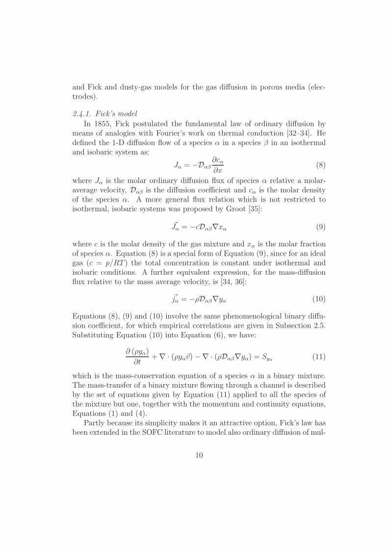
2.4.1. Fick’s model

In 1855, Fick postulated the fundamental law of ordinary diffusion bymeans of analogies with Fourier’s work on thermal conduction [32–34]. Hedefined the 1-D diffusion flow of a species α in a species β in an isothermaland isobaric system as:

Jα = −Dαβ∂cα∂x

(8)

where Jα is the molar ordinary diffusion flux of species α relative a molar-average velocity, Dαβ is the diffusion coefficient and cα is the molar densityof the species α. A more general flux relation which is not restricted toisothermal, isobaric systems was proposed by Groot [35]:

~Jα = −cDαβ∇xα (9)

where c is the molar density of the gas mixture and xα is the molar fractionof species α. Equation (8) is a special form of Equation (9), since for an idealgas (c = p/RT ) the total concentration is constant under isothermal andisobaric conditions. A further equivalent expression, for the mass-diffusionflux relative to the mass average velocity, is [34, 36]:

~jα = −ρDαβ∇yα (10)

Equations (8), (9) and (10) involve the same phenomenological binary diffu-sion coefficient, for which empirical correlations are given in Subsection 2.5.Substituting Equation (10) into Equation (6), we have:

∂ (ρyα)

∂t+∇ · (ρyα~v)−∇ · (ρDαβ∇yα) = Syα (11)

which is the mass-conservation equation of a species α in a binary mixture.The mass-transfer of a binary mixture flowing through a channel is describedby the set of equations given by Equation (11) applied to all the species ofthe mixture but one, together with the momentum and continuity equations,Equations (1) and (4).

Partly because its simplicity makes it an attractive option, Fick’s law hasbeen extended in the SOFC literature to model also ordinary diffusion of mul-

10

ticomponent mixtures in the channels, and to model simultaneously ordinaryand Knudsen diffusion in the electrodes [22, 23, 37]. Both approximationsare detailed below.

The diffusion coefficient of a species α in a multicomponent gas system(Dαm) is given by:

Dαm =1− xα

∑

β 6=α

(

xβ

Dαβ

) (12)

Equation (12) stems from the Stefan-Maxwell equations [38] and was exper-imentally verified by Fairbanks and Wilke [39]. From Equations (10) and(12), the Fickian law for the ordinary diffusion flux of the species α in amulticomponent mixture is:

~jα = −ρDαm∇yα (13)

Replacing Equation (13) into Equation (6), the mass-conservation equationof the species α in a multicomponent mixture, according to a Fickian law ofdiffusion, is given by:

∂ (ρyα)

∂t+∇ · (ρyα~v)−∇ · (ρDαm∇yα) = Syα (14)

Similarly,an effective global-diffusion coefficient of species α in a porousmedium, Dα

eff , may be derived [33] as:

1

Deffα

=1−Υxα

Deffαm

+1

DeffKα

(15)

In previous SOFCs simulation works [22, 23, 37, 38, 40] Υ is assumed tobe zero, despite this being only strictly true for self-diffusion or equimolarcounter transfer [33]; then Equation (15) becomes:

1

Deffα

=1

Deffαm

+1

DeffKα

(16)

Here, Deffαm is the effective binary diffusion coefficient of species α in the

mixture in the porous medium:

Deffαm =

ε

τDαm (17)

11

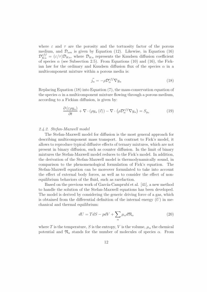
where ε and τ are the porosity and the tortuosity factor of the porousmedium, and Dαm is given by Equation (12). Likewise, in Equation (16)Deff

Kα = (ε/τ)DKα, where DKα represents the Knudsen diffusion coefficientof species α (see Subsection 2.5). From Equations (10) and (16), the Fick-ian law for the ordinary and Knudsen diffusion flux of the species α in amulticomponent mixture within a porous media is:

~jα = −ρDeffα ∇yα (18)

Replacing Equation (18) into Equation (7), the mass-conservation equation ofthe species α in a multicomponent mixture flowing through a porous medium,according to a Fickian diffusion, is given by:

∂ (ερyα)

∂t+∇ · (ρyα 〈~v〉)−∇ ·

(

ρDeffα ∇yα

)

= Syα (19)

2.4.2. Stefan-Maxwell model

The Stefan-Maxwell model for diffusion is the most general approach fordescribing multicomponent mass transport. In contrast to Fick’s model, itallows to reproduce typical diffusive effects of ternary mixtures, which are notpresent in binary diffusion, such as counter diffusion. In the limit of binarymixtures the Stefan-Maxwell model reduces to the Fick’s model. In addition,the derivation of the Stefan-Maxwell model is thermodynamically sound, incomparison to the phenomenological formulation of Fick’s equation. TheStefan-Maxwell equation can be moreover formulated to take into accountthe effect of external body forces, as well as to consider the effect of non-equilibrium behaviors of the fluid, such as rarefaction.

Based on the previous work of Garcıa-Camprubı et al. [41], a new methodto handle the solution of the Stefan-Maxwell equations has been developed.The model is derived by considering the generic driving force of a gas, whichis obtained from the differential definition of the internal energy (U) in me-chanical and thermal equilibrium:

dU = TdS − pdV +∑

α

µαdNα (20)

where T is the temperature, S is the entropy, V is the volume, µα the chemicalpotential and Nα stands for the number of molecules of species α. From

12

Equation (20) we can express the variation of entropy as:

dS =

(

1

T

)

dU +( p

T

)

dV +∑

α

(

−µα

T

)

dNα (21)

where (1/T ), (p/T ) and (−µα/T ) are the thermal, mechanical and chemicaldrivers respectively. Considering an ideal gas, a single component and theEuler’s homogeneous function theorem applied to the extensive thermody-namic variables, Equation (21) yields:

d(µα

T

)

= −Cv,α

TdT +

R

nαdnα (22)

where nα = Nα/V , Cv,α is the heat capacity at constant volume of species α,and R is the ideal-gas law constant. The integration of Equation (22) yields:

−µα

T= Cv,αln

(

T

T0

)

− Rln

(

nα

n0

)

(23)

being n0 and T0 arbitrary constants. The thermodynamic definition of thediffusion driver, for the isothermal case with T0 = T , considering n0 = 1 andlinearizing the solution around T0, is given by: µα/T = Rpα, where pα is thepartial pressure of the species α. Therefore, we obtain:

∇(µα

T

)

T= R∇pα (24)

Notice that this is strictly valid for the isothermal case and for those non-isothermal cases where thermodiffusion is negligible. From an asymptoticexpansion as a function of the Knudsen number [42], the partial-pressuregradient can be expressed as the sum of the pressure gradients due to diffusiveand viscous effects:

∇pα = ∇pdα +∇pvα (25)

An expression for the diffusive effects is obtained from the balance betweenthe driving force and the friction between molecules of different species [43]:

∇pdα = p∑

β 6=α

xαxβDαβ

(~vβ − ~vα) (26)

13

which is the Stefan-Maxwell equation for the diffusive flux of a multicompo-nent mixture, where xα is the molar fraction of species α, ~vα is the velocityof the species α, and α and β stands for all the gaseous components of themixture. On the other hand, the viscous component of the partial-pressuregradient appears in the momentum equation for the species:

ρα

(

D~vαDt

− ν∇2~vα

)

+∇pvα = ρα~aα (27)

where ρα = ρyα, D/Dt is the substantial derivative, ν is the kinematic vis-cosity of the fluid and ~aα is the acceleration of the species α due to thepresence of external forces. The sum, extended to all the species in the fluid,of Equation (27) yields:

ρ

(

D~v

Dt− ν∇2~v

)

+∇p =∑

α

ρα~aα (28)

In the diffusive limit we have:

D~vαDt

− ν∇2~vα ≈ D~v

Dt− ν∇2~v =

1

ρ

(

∑

α

ρα~aα −∇p)

(29)

From Equations (27) and (29), the viscous part of the partial-pressure gra-dient can be thus expressed as:

∇pvα = yα∇p+ ρα

(

~aα −∑

α

yα~aα

)

(30)

From Equation (25), recasting Equation (26) in terms of the molar fluxes(

~Nα = cα~vα

)

and considering Equation (30) for an inertial system (~aα = 0),

we obtain:1

RT∇pα =

∑

β 6=α

xα ~Nβ − xβ ~Nα

Dαβ

+1

RTyα∇p (31)

which is the Stefan-Maxwell equation consistent with the momentum equa-tion, Equation (1). From Equation (31):

~Nα = −ΓSM

α ∇pα + ~υpSM

α pα + ~υNSM

α pα (32)

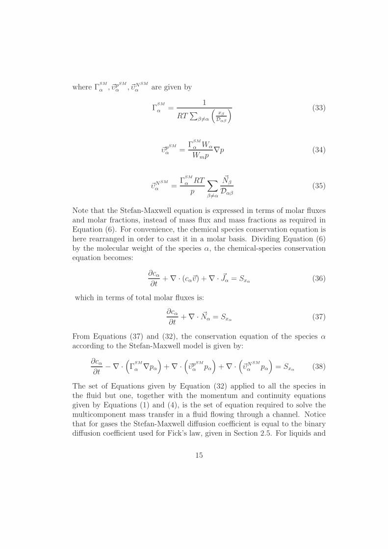
14

where ΓSM

α , ~υpSM

α , ~υNSM

α are given by

ΓSM

α =1

RT∑

β 6=α

(

xβ

Dαβ

) (33)

~υpSM

α =Γ

SM

α Wα

Wmp∇p (34)

~υNSM

α =Γ

SM

α RT

p

∑

β 6=α

~Nβ

Dαβ(35)

Note that the Stefan-Maxwell equation is expressed in terms of molar fluxesand molar fractions, instead of mass flux and mass fractions as required inEquation (6). For convenience, the chemical species conservation equation ishere rearranged in order to cast it in a molar basis. Dividing Equation (6)by the molecular weight of the species α, the chemical-species conservationequation becomes:

∂cα∂t

+∇ · (cα~v) +∇ · ~Jα = Sxα(36)

which in terms of total molar fluxes is:

∂cα∂t

+∇ · ~Nα = Sxα(37)

From Equations (37) and (32), the conservation equation of the species αaccording to the Stefan-Maxwell model is given by:

∂cα∂t

−∇ ·(

ΓSM

α ∇pα)

+∇ ·(

~υpSM

α pα

)

+∇ ·(

~υNSM

α pα

)

= Sxα(38)

The set of Equations given by Equation (32) applied to all the species inthe fluid but one, together with the momentum and continuity equationsgiven by Equations (1) and (4), is the set of equation required to solve themulticomponent mass transfer in a fluid flowing through a channel. Noticethat for gases the Stefan-Maxwell diffusion coefficient is equal to the binarydiffusion coefficient used for Fick’s law, given in Section 2.5. For liquids and

15

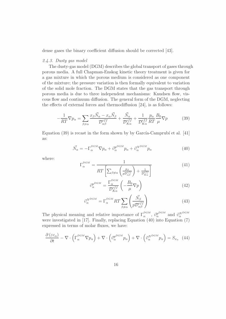
dense gases the binary coefficient diffusion should be corrected [43].

2.4.3. Dusty gas model

The dusty-gas model (DGM) describes the global transport of gases throughporous media. A full Chapman-Enskog kinetic theory treatment is given fora gas mixture in which the porous medium is considered as one componentof the mixture; the pressure variation is then formally equivalent to variationof the solid mole fraction. The DGM states that the gas transport throughporous media is due to three independent mechanisms: Knudsen flow, vis-cous flow and continuum diffusion. The general form of the DGM, neglectingthe effects of external forces and thermodiffusion [24], is as follows:

− 1

RT∇pα =

∑

β 6=α

xβ ~Nα − xα ~Nβ

Deffαβ

+~Nα

DeffKα

+1

DeffKα

pαRT

B0

µ∇p (39)

Equation (39) is recast in the form shown by by Garcıa-Camprubı et al. [41]as:

~Nα = −ΓDGM

α ∇pα + ~υpDGM

α pα + ~υNDGM

α pα (40)

where:

ΓDGM

α =1

RT

[

∑

β 6=α

(

pβ

pDeffαβ

)

+ 1

DeffKα

] (41)

~υpDGM

α =Γ

DGM

α

DeffKα

(

−B0

µ∇p)

(42)

~υNDGM

α = ΓDGM

α RT∑

β 6=α

(

~Nβ

pDeffαβ

)

(43)

The physical meaning and relative importance of ΓDGM

α , ~υpDGM

α and ~υNDGM

α

were investigated in [17]. Finally, replacing Equation (40) into Equation (7)expressed in terms of molar fluxes, we have:

∂ (εcα)

∂t−∇ ·

(

ΓDGM

α ∇pα)

+∇ ·(

~υpDGM

α pα

)

+∇ ·(

~υNDGM

α pα

)

= Sxα(44)

16

which is the chemical-species conservation-equation in the porous media ac-cording to the dusty gas model. Equation (44) applied to all the componentsof the gas mixture represents the complete set of equations for steady-statemass transport, and does not need to be supplemented by any additionalequations of motion [24].

The DGM is considered to be the most convenient approach to model thegas transport through porous media [43] and within the SOFC electrodes[20]. Therefore, it is increasingly used for SOFC modeling [13, 17]. However,it is worth noting that the theoretical basis of the DGM [24] was criticizedby Kerkhof in [44, 45], who as an alternative proposed the binary-frictionmodel (BFM). The experimental data of Evans et al. [46, 47] were used tovalidate the BFM and the DGM; both models showed similar agreement anddiscrepancies with the measured data [44]. Moreover, Vural et al. [48] haverecently reported similar predictions of both models for the concentrationoverpotential of a SOFC.

2.5. Diffusion-coefficient modeling

Experimental data for diffusivities is scarce and the diffusion coefficientsmust be often calculated using the theoretical or empirical correlations intro-duced in this Subsection. Nevertheless, experimental diffusivity values mustbe used, when possible, because measurement errors are typically less thanthose associated with the predictions of empirical or even semi-theoreticalequations [49]. In the present work, the measured data for Dαβ and DKα

may be directly taken as a constant.

2.5.1. Champan-Enskog model

The Chapman-Enskog correlation, based on the Kinetic Theory of Gases,is the most common method for theoretically estimating the binary diffusivity[34, 50]. It has been widely used for SOFC simulation [21, 51, 52]. Theoriginal expression of the Chapman-Enskog correlation is:

Dαβ =0.001858T 1.5

(

1Wα

+ 1Wβ

)0.5

pσ2αβΩD

(45)

where Dαβ is given in square centimeters per second, the temperature inKelvin, the molecular weight of species α in kilogram per kilomole and thetotal pressure in atmospheres; the average collision diameter in angstroms,

17

calculated as:

σαβ =σα + σβ

2(46)

where the value of σα is tabulated for the most common species in [53]; andΩD is the dimensionless collision integral in the Lennard-Jones 12-6 potentialmodel:

ΩD =1.06036

TN0.15610+

0.19300

exp(0.47635TN)+

1.03587

exp(1.52996TN)+

1.76474

exp(3.89411TN)(47)

Here:

TN =T

Eαβ(48)

with T the temperature and Eαβ = εαβ/kB; kB is the Boltzmannn constant,εαβ = (

√εαεβ); and εα is the characteristic Lennard-Jones energy. For the

most common gases the value of Eαβ is tabulated in [53].For convenience we define a new variableWαβ, which represents an equivalentmolecular weight of the species α and β:

Wαβ =

(

1

Wα+

1

Wβ

)−1

=WαWβ

Wα +Wβ(49)

Replacing Equation (49) into Equation (45) we have:

Dαβ =0.001858T 1.5 (Wαβ)

−0.5

pσ2αβΩD

(50)

Because of unit consistency, Equation (50) is modified as follows:

Dαβ = 10.13250.001858T 1.5 (Wαβ)

−0.5

pσ2αβΩD

(51)

Equation (51) differs from Equation (45) in the units of the total pressureand the binary diffusion coefficient; here, SI units apply (Pa, m2s−1).

18

2.5.2. Wilke-Lee model

The Wilke-Lee correlation for the binary diffusion model is given by [54]:

Dαβ =

(

0.0027− 0.0005(

Wα+Wβ

WαWβ

)0.5)

T 1.5(

Wα+Wβ

WαWβ

)0.5

pσ2αβΩD

(52)

where Dαβ is expressed in square centimeters per second, the molecularweight is expressed in kilogram per kilomole, the temperature is in Kelvin,and the pressure is in atmospheres; σαβ is defined in Equation (46) wherethe collision diameters must be introduced in angstroms; and the collisionintegral (dimensionless) is defined by Equation (47).Introducing Equation (49) into Equation (52) we have:

Dαβ =

(

0.0027− 0.0005W−0.5αβ

)

T 1.5W−0.5αβ

pσ2αβΩD

(53)

To convert the units of the binary ordinary-diffusion coefficient and the pres-sure into the SI system (m2s−1, Pa) Equation (53) is modified as follows:

Dαβ = 10.1325

(

0.0027− 0.0005W−0.5αβ

)

T 1.5W−0.5αβ

pσ2αβΩD

(54)

where σαβ is the only parameter that is not expressed in SI system units, asit remains in angstroms.

2.5.3. Fuller-Schettler-Giddings model

The Fuller-Schettler-Giddings empirical correlation is the simplest cor-relation to use and it is reported to be more accurate for the prevailingSOFC operating conditions [55]; it is thus widely used for SOFCs simula-tion [14, 16, 37]. The Fuller-Schettler-Giddings empirical correlation for thebinary diffusivity (Dαβ) of non-polar gases at low pressures is [34, 56]:

Dαβ =0.001T 1.75

(

1Wα

+ 1Wβ

)0.5

p[

(Σv)α1/3 + (Σv)β

1/3]2 (55)

19

where Σv is the diffusion volume, Dαβ is given in square centimeters persecond, the temperature in Kelvin, the molecular weight of the species-α inkilogram per kilomole and the total pressure in atmospheres; the value of thediffusion volume of species α (

∑

vα) is tabulated in [33, 34].Substituting Equation (49) into Equation (55) we have:

Dαβ =0.001T 1.75W−0.5

αβ

p[

(Σv)α1/3 + (Σv)β

1/3]2 (56)

To convert Equation (56) to use consistent units, it is modified as follows:

Dαβ = 10.13250.001T 1.75W−0.5

αβ

p[

(∑

v)α1/3 + (

∑

v)β1/3]2 (57)

where the SI units are now used for all the variables involved. Hence, inEquation (57) the binary diffusion coefficient is expressed in square metersper second, the temperature in Kelvin; the molecular weight in kilogram perkilomole, and the total pressure in Pascal.

2.5.4. Knudsen model

The Kinetic Theory of Gases defines the Knudsen diffusion coefficient as[33, 50]:

DKα=dp3

√

8RT

π Wα

(58)

where DKαis given in SI units if the temperature is expressed in Kelvin, the

molecular weight in kilograms per kilomole, the mean pore diameter (dp) inmeters and the ideal gas law constant in Joule per kilomole per Kelvin. Equa-tion (58) is unanimously used for the calculation of the Knudsen diffusivityin the SOFC related literature.

3. Overview of the software structure

In the modeling and simulation of phenomena of scientific and techno-logical relevance, open source codes offer a collaborative platform for thedissemination of new ideas and methodologies and, simultaneously, fosterthe optimal evolution of state-of-the-art algorithms due to the peer review

20

and control of the source code itself. These benefits speed up the develop-ment of design tools and boost the collaboration between code developersand equipment designers, and their mutual feedback.

The work presented in this paper is based on the OpenFOAMR© toolbox,an open-source platform for the solution of partial differential equations usu-ally encountered in the mathematical description of continuum mechanics ofsolids and fluids. This toolbox is an implementation of fast, robust and accu-rate numerical solvers designed for managing complex geometries using thefinite-volume method. It uses the natural language of continuum mechanics,representing the equations in a straightforward way, as shown in Algorithm 1.

OpenFOAMR© has an object-oriented design and is written in C++, whichprovides one of its most useful features: the extension of the modeling ca-pabilities in the form of libraries, such as the one introduced in this paperand intended to address the simulation of SOFCs. It encompasses two sep-arate items. These are: a library (Section 4.1) embodying the mass-transfermodels; and a solver (Section 4.2), which handles the definition of the SOFCdomains, the SOFC models and their coupling.

4. Description of the individual software components

4.1. Multispecies mass-transfer library

Multispecies mass-transport is not only a key submodel in a SOFC simula-tion but it is also required for the numerical solution of a wide range of indus-trial processes (eg catalytic converters, or chemical-vapor deposition). How-ever, OpenFOAMR© does not include a general multispecies mass-transportcode (as of version 1.6-ext or 1.7.x). To fill this gap, the authors have devel-oped a multispecies mass-transfer library following the OpenFOAMR© conven-tions and philosophy. The library contains the most widely used multispeciesmass-transport models in the literature, which were introduced in Section 2.A graphical description of the library contents and structure is shown inFigure 2; it is is divided in four major blocks described below.

4.1.1. Thermophysical models

The thermoPhysicalModels is the library database, and consists of thefollowing classes: (i) multiComponentMixtureMassBases; and (ii)multiComponentMixtureMolarBases.

Both classes store all the required variables to characterize a mixture ofspecies α (yα , xα , nα , Nα andWm) as well as the functions correct and the

21

functions to update the fluxes (correctMolarFluxes and correctMassFluxesrespectively). As it is shown in Section 2.4, the species mass conservationequation changes depending on the chosen diffusion model, as it also doesthe dependent variable to be solved (yα for fickian models and pα for Stefan-Maxwell and dusty-gas models). Therefore, each diffusion model recalls theproper mixture class (models that use pα are based on multiComponentMixtureMolarBases).The function correct contains the correlations needed to calculate the mix-ture molar weight and the remain composition variables (from mass fractionsto molar fractions for multiComponentMixtureMassBases and from molarfractions to mass fractions for multiComponentMixtureMolarBases). Bothclasses work like a base for a standard OpenFOAMR© thermodynamic modelin witch all mixture properties are defined (cp, α, etc...).

4.1.2. Momentum-continuity models

This block is based on the class momentumTransport, which includes thestructure to account for momentum and mass conservation. The derivedclasses are: (i) SIMPLE; (ii) porousSIMPLE; and (iii) Darcy.

SIMPLE contains the code to solve Equations (1) and (4) using the SIM-PLE velocity-pressure algorithm implemented in rhoSimpleFoam, an stan-dard solver of OpenFOAMR©.

porousSIMPLE solves Equations (2) and (5) as it is done in the standardOpenFOAMR© solver rhoPorousSimpleFoam.

Darcy solves Equations (3) that is the common form of the Darcy Law.

4.1.3. Mass-transfer models

In Algorithm 2, the structure of the class multiSpeciesTransportModelis shown. This handles the solution of the chemical species conservationequation for a given diffusion model (see Section 2.4) either in a channel orin a porous media. The derived classes from multiSpeciesTransportModel,named after the mass-diffusion model, are: (i) Fick ; (ii) MaxwellStefan;and (iii) dustyGas.

The Fick class allows the user to specify which of the three possible Fick-ian species-conservation equations must be considered: Equation (11) for bi-nary mixtures; Equation (14) for multicomponent mixtures; or Equation (19)for multicomponent mixtures in a porous medium. As shown in Algorithm 2,the procedure of this subroutine is as follows: (a) it solves the momentumand continuity equations, calling the class momentumTransport::SIMPLE ormomentumTransport::porousSIMPLE depending on the medium; (b) it solves

22

the selected mass-conservation equation for (N − 1) species; (c) it calculatesthe total mass fluxes, ~nα; (d) it calculates the value of the non-solved-forspecies ensuring continuity; (e) it updates the the molar bases fields, call-ing the update functions of multiComponentMixtureMassBases; and (f) itupdates the diffusion coefficients with the class diffusivityModel.

The MaxwellStefan class allows the solution of the multicomponent mass-transfer in a porosity-free domain. The algorithm, also shown in Algorithm 2,is: (a) the class momentumTransport::SIMPLE is called to solve the momen-tum and continuity equations; (b) Equation (38) is solved for (N−1) species;

(c) the total molar fluxes, ~Nα, are calculated; (d) the value of the non-solved-for species is calculated ensuring continuity; (e) molar fractions are calcu-lated from partial pressures; (f) multiComponentMixtureMolarBases updatefunctions are called to update the mass fields; (g) class diffusivityModelis called to update the diffusion coefficients; and (h) the parameters of thespecies conservation equation (Γ

SM

α , ~υpSM

α , ~υNSM

α ) are recalculated.The dustyGas class contains the algorithm to solve the mass transport

through a porous media according to the dusty-gas model. It differs fromthe ones used in the Fick and MaxwellStefan classes in that it admits onlymomentumTransport::Darcy. The procedure, shown in Algorithm 2 is: (a)Equation (44) is solved for all the species of the gas mixture; (b) the total mo-

lar fluxes, ~Nα, are calculated; (c) the total pressure of the fluid is calculatedas: p =

∑

α pα; (d) molar fractions are calculated from partial pressures;(e) multiComponentMixtureMolarBases update functions are called to up-date the mass fields; (f) the diffusivities are recalculated calling the classdiffusivityModel; (g) Γ

DGM

α , ~υpDGM

α , ~υNDGM

α are updated; and blue(h) thefluid permeation velocity is calculated from Equation (44).

For the proper performance of the library, a new boundary condition,called fixedFlux, is required. fixedFlux is derived from the OpenFOAMR©

basic boundary-condition fixedGradientFvPatchField and its implemen-tation follows the standard OpenFOAMR© conventions in order to obtain ageneric boundary condition applicable for all mass-transport models. Given ageneric mass-flux of a species α normal to a boundary surface (ψα), fixedFluxcalculates the normal gradient of the species (snGradφα

) at that boundaryaccording to the chosen diffusion model:

snGradφα=

(υNα + υpα) φα − ψα

Γα. (59)

23

where φα, ψα, υNα , υpα and Γα for the different diffusion models are given in

Table 1.

4.1.4. Diffusion-coefficient models

The diffusivityModel is the generic class to compute the diffusivity co-efficients. The theoretical or semi-empirical correlations described in Section2.5 have been implemented in the derived classes: (i) constant to intro-duce experimental diffusivity values; (ii) Champan-Enskog to calculate Dαβ

according to Equation (51); (iii) Wilke-Lee to calculate Dαβ according toEquation (54); (iv) Fuller-Schettler-Giddings to calculate Dαβ accord-ing to Equation (57); and (v) Knudsen to calculate DKα, given by Equation(58). The user may select at run time which model to use.

4.2. SOFC solver

The SOFC solver is a CFD tool to simulate the performance of a solidoxide fuel cell. The solver has been also written in C++, taking into accountthe OpenFOAMR© code style and fully ensuring its compatibility. The SOFCsolver represents an example of the capability of the previously describedmulti-species mass-transport library and it can be further extended by linkingit to other libraries (eg an eventual thermal sub-model).

The main feature of the SOFC solver is that it divides the SOFC in fiveadjacent subdomains, according to its different components: (i) fuel channel;(ii) anode; (iii) electrolyte; (iv) cathode; and (v) air channel. The solverrequires one mesh for each of those subdomains to solve the physical phe-nomena taking place in each component; and thus it also requires a couplingalgorithm to transfer information from each mesh to its neighbouring ones.

The SOFC solver structure is based on a virtual class called component,from which two classes are derived: (i) solidComponent to store the proper-ties of a solid material in a class material; and (ii) fluidComponent whichcontains the functions to exchange fluid fields between regions. Since aSOFC component may be a fluid, a solid or a mixture of both (eg fluidflowing through a porous medium), the following classes have been furtherderived to model each of the cell components: (a) channel derived fromfluidComponent to model the gas channels (either air or fuel channel); (b)electrode to model the porous media of the cell (anode or cathode), it isthus derived from both fluidComponent and solidComponent; and (c) aclass electrolyte derived from solidComponent to model the impervioussolid in the cell (the electrolyte).

24

Classes channel and electrode inherit the mass and momentum conser-vation algorithms from classes multiSpeciesTransportModel and momentumTransport(see Section 4.1). Since the electrochemical reaction in a SOFC takes placein a very thin region in the vicinity of the electrode-electrolyte interfaces[57], it is considered to take place on a surface and it is thus modeled as aboundary condition, where the gradient of each component of the mixture iscalculated applying the fixedFlux boundary condition to the molar fluxesgiven by Faraday’s Law:

~Nα,r · ~nr =I

nF(60)

where I is the current density, ~nr is the unit vector normal to the reactionboundary, n is the number of electrons required to convert a single moleculeof species α and F is Faraday’s constant. Since no volumetric reactionsare considered, the following relationships are valid at every cell component:Sxα

= 0, Syα = (SxαWα) = 0, Sy = (

∑

α Syα) = 0. However, when using theboundary condition fixedFlux special care must be taken at the reactionboundaries (electrode-electrolyte interfaces), where the velocity is fixed to

zero (electrolyte is an impervious solid) and then ~Nα,r = ~Jα,r. It should be

noted that∑

α(Wα~Jα,r) 6= 0, ie

∑

α(~jα,r) 6= 0. The reaction boundaries are

mass-diffusion inlet-outlets of the cell. This diffusivity-boundary mass sourceis therefore taken into account when solving the continuity equation in themomentumTransport (surfMassSource).

On the other hand, mass transport is not solved in the electrolyte, wherethe conservation of anions is imposed. Therefore, the class electrolyte doesnot contain any multiSpeciesTransportModel or momentumTransport asthe other components do. However, electrolyte stores the electrochemicalalgorithm to solve the electrochemistry of the cell; it is based on the one de-scribed in [58]. The electrolyte is modeled like a thin plate, where the currentdensity path is normal to the electrolyte-electrode interface. Either the cellcurrent density or the cell voltage is required as an input in the electrolyteclass. If the cell voltage is given, the function updateCurrentDensity()

solves the Butler-Volmer equation and the Ohm law for each element of themesh to find the current density value that satisfies the imposed voltage. If,on the contrary, the average current density is fixed, then a similar subroutineupdateVoltage() calculates the cell voltage.

All the above mentioned classes are combined in a top level solver, namedsofcFoam, that defines the procedure for the solution of the SOFC solver.

25

Figure 3 shows the flow chart of the SOFC solver algorithm and coupling; andTable 2 gathers the boundary conditions required by the solver. Essentially,sofcFoam reads from a file the regions names and creates the respective ob-jects. All these objects are independent and can be independently controlledboth in terms of the selection of submodels and of solution parameters. Thesolution algorithm is segregated and the most convenient order to solve re-gions is starting from the inner of the cell. Thus, the electrolyte is solved first,then the electrodes, and finally the gas channels; the process is repeated untilconvergence. Every time a region is solved, the corresponding elements inthe neighbouring mesh are updated using the OpenFOAMR© autoMap class.

5. Validation and Results

5.1. Validation of the multi-species mass-transfer library

The performance of the mass-transfer library presented in Section (4.1)is here assessed by comparison with analytical solutions of the mass-transfermodels presented in Section 2.4. For this purpose, the well-known StefanTube test case (1D, steady-state, multicomponent mass-transfer at constantpressure) is used. Note that in this section the mass or molar fluxes (either

~nα or ~Nα) are one-dimensional vectors, in the direction of the tube axis;therefore only the magnitude of the vector is used in the derivation of theanalytical solutions (nα or Nα).

5.1.1. Validation of Fick

The analytical solution of Equation (11) for a non-reacting binary mixtureis:

yα(x) =

nαWα

nαWβ+nβWα+ yα(0)Wα

yα(0)(Wβ−Wα)+Wα− nαWα

nαWβ+nβWαe(

(nαWβ+nβWα)RTx

WβWαpDαβ)

1− nα(Wβ−Wα)

nαWβ+nβWα− yα(0)(Wβ−Wα)

yα(0)(Wβ−Wα)+Wα− nα(Wβ−Wα)

nαWβ+nβWαe(

(nαWβ+nβWα)RTx

WβWαpDαβ)

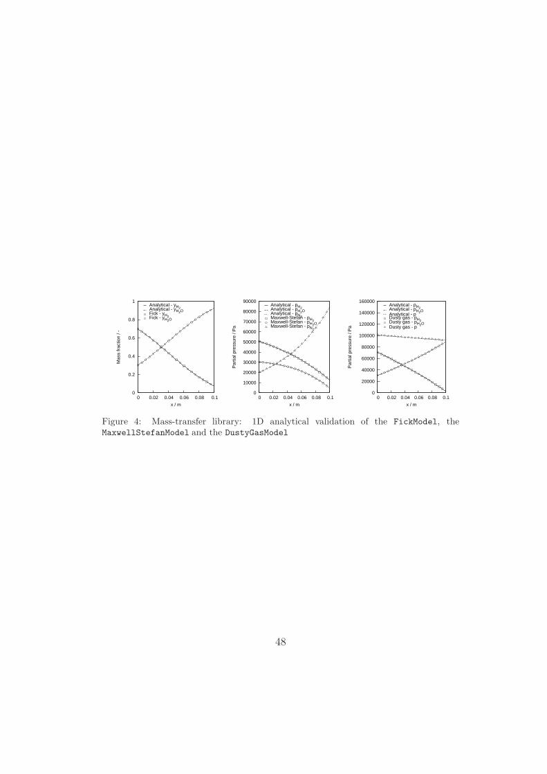
(61)where the following relationships have been used: nα = yαρv − ρDαβ∇yα,yα+yβ = 1, ρ = pWm/(RT ) and Wm =WαWβ/(yα(Wβ−Wα)+Wα). Figure4 shows the comparison between the numerical results obtained with thelibrary and the analytical results calculated with Equation (61), under theconditions given in Table 3.

26

5.1.2. Validation of MaxwellStefan

From Equation (31) the Stefan-Maxwell equations for the steady-statemulticomponent diffusion under constant pressure are:

∇pα = RT∑

β

~Nβ pα − ~Nα pβpDα,β

(62)

For the Stefan Tube test (1D), we can write Equation (62) in matrix formas follows:

dpαdx

= Dα,β pα +Mα (63)

Defining Λα,β = Sα,β Dα,β S−1α,β, where Λα,β is a diagonal matrix containing the

eigenvalues (λα) of the matrix Dα,β, and Sα,β is the corresponding eigenvec-tors matrix, and using the auxiliary variables qα = Sα,β pα andGα = Sα,β Mα,the system of Equations (63) can be written in the form:

dqαdx

= λα qα(x) +Gα (64)

the solution of which is:

qα(x) =

[

qα(0) +Gα

λα

]

exp(λαx)−Gα

λα(65)

In the case of a ternary mixture (species: α, β, γ) in 1D, the system of Equa-tions (62) may be expressed as:

dpαdx

=RT

p

[(

Nα +Nγ

Dαγ

+Nβ

Dαβ

)

pα +

(

Nα

Dαγ

− Nα

Dαβ

)

pβ −Nα

Dαγ

p

]

(66)

dpβdx

=RT

p

[(

Nβ

Dβγ− Nβ

Dαβ

)

pα +

(

Nβ +Nγ

Dβγ+

Nα

Dαβ

)

pβ −Nβ

Dβγp

]

(67)

pγ = p− pα − pβ (68)

27

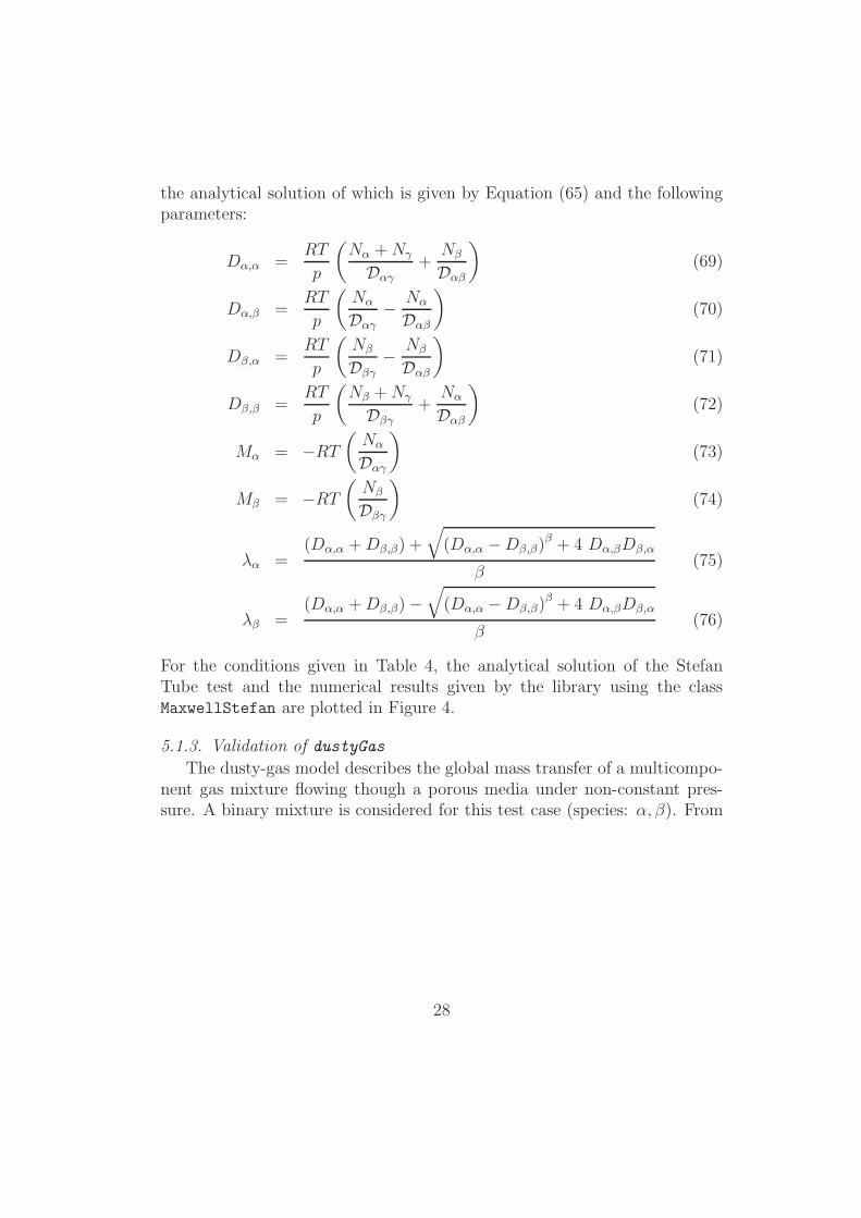
the analytical solution of which is given by Equation (65) and the followingparameters:

Dα,α =RT

p

(

Nα +Nγ

Dαγ+

Nβ

Dαβ

)

(69)

Dα,β =RT

p

(

Nα

Dαγ− Nα

Dαβ

)

(70)

Dβ,α =RT

p

(

Nβ

Dβγ− Nβ

Dαβ

)

(71)

Dβ,β =RT

p

(

Nβ +Nγ

Dβγ+

Nα

Dαβ

)

(72)

Mα = −RT(

Nα

Dαγ

)

(73)

Mβ = −RT(

Nβ

Dβγ

)

(74)

λα =(Dα,α +Dβ,β) +

√

(Dα,α −Dβ,β)β + 4 Dα,βDβ,α

β(75)

λβ =(Dα,α +Dβ,β)−

√

(Dα,α −Dβ,β)β + 4 Dα,βDβ,α

β(76)

For the conditions given in Table 4, the analytical solution of the StefanTube test and the numerical results given by the library using the classMaxwellStefan are plotted in Figure 4.

5.1.3. Validation of dustyGas

The dusty-gas model describes the global mass transfer of a multicompo-nent gas mixture flowing though a porous media under non-constant pres-sure. A binary mixture is considered for this test case (species: α, β). From

28

Equation (39) the following system of equations is obtained:

dp

dx= −

RT(

Nα

DKα+

Nβ

DKβ

)

1 + B0

µ

[

pα

(

1DKα

− 1DKβ

)

+ pDKβ

] (77)

dpαdx

=RT

pD12[pα (Nα +Nβ)− pNα]−

RT

pDKα

Nα − pαB0

µDKα

∇p (78)

dpβdx

=dp

dx− dpα

dx(79)

This system is solved numerically by scripting the solution procedure in Oc-tave [59, 60]. Figure 4 also shows the comparison between the analyticalcurves and the numerical results for the dustyGas for the conditions givenin Table 5.

Figure 5 shows the relative errors (ζ) between the reference solutions(analytical or numerical) and the results calculated in this work for all thetest cases presented in this section and their dependency with the mesh size.The error is calculated as:

ζ =φref − φOpenFOAM

φref

(80)

The results shown in Figure 5 further validate the performance of the library.

5.2. SOFC solver results and validation

The performance of the sofcFoam application introduced in Section 4.2is shown now by comparison with the experimental data of a circular-shape,planar SOFC; the experimental data have been collected in the authors’(VN, PA) laboratory. The geometry and properties of the cell, as well asthe operating conditions, are reported in Table 6. Two approaches for therepresentation of the cell will be considered: (i) 2D simulations assumingaxial symmetry; (iii) full 3D simulations. Figures. 6 and 7 show some detailsof the meshes used for both approaches. The meshes were successively refineduntil the numerical results indicated no dependence on the mesh, as shownin Figure 8.

Figure 9 shows the experimental and numerical I-V curves for the cellgiven in Table 6 at three different operating temperatures. The model fitting

29

parameter is the pre-exponential factor of the cathode current exchange den-sity, which is not kept constant from curve to curve because it is temperaturedependent. Good agreement is reached between numerical and experimentaldata, for both the 2D and 3D simulations.

6. Practical issues

6.1. Installation instructions

The package multiSpeciesTransportModels consists in three folders, namelylib, applications and run and requires a fully functionally installation ofOpenFOAMR© (version 1.6-ext). In order to install the main software easily,under Ubuntu Lucid 10.04 LTS it is sufficient to add the PPA repositorytyping in a terminal (superuser privileges are required):

sudo add-apt-repository ppa:cae-team/ppa

and then

sudo apt-get update

sudo apt-get install openfoam-1.6-ext

sudo apt-get install openfoam-1.6-ext-dev

sudo apt-get install binutils-dev

sudo apt-get install g++

sudo apt-get install cmake

to install the package satisfying all the dependencies. Finally by typing

echo ". /usr/lib/OpenFOAM-1.6-ext/etc/bashrc"

>> ~/.bashrc

echo "export FOAM_USER_APPBIN=

$WM_PROJECT_USER_DIR/applications/bin/$WM_OPTIONS"

>> ~/.bashrc

30

echo "export FOAM_USER_LIBBIN=

$WM_PROJECT_USER_DIR/lib/$WM_OPTIONS"

>> ~/.bashrc

echo "export PATH=$PATH:$FOAM_USER_APPBIN"

>> ~/.bashrc

echo "export LD_LIBRARY_PATH=

$LD_LIBRARY_PATH:$FOAM_USER_LIBBIN"

>> ~/.bashrc

source ~/.bashrc

the installation process will be completed. To install OpenFOAMR© underother operating system or to compile it from the source code one can refer theinstructions reported on the main web site (http://www.extend-project.de).Now for install the multiSpeciesTransportModels create the OpenFOAMR©

user home folder (if not present) and subfolders with the commands

mkdir ~/OpenFOAM

mkdir ~/OpenFOAM/$USER-1.6-ext

mkdir ~/OpenFOAM/$USER-1.6-ext/lib

mkdir ~/OpenFOAM/$USER-1.6-ext/applications

mkdir ~/OpenFOAM/$USER-1.6-ext/run

and extract the package in temporary directory (i.e. ˜/temp-install) with

tar -zxvf multiSpeciesTransportModels.tar.gz

Finally by typing

cp -r ~/temp-install/mstm/lib/*

~/OpenFOAM/$USER-1.6-ext/lib

cp -r ~/temp-install/mstm/applications/*

31

~/OpenFOAM/$USER-1.6-ext/applications

cp -r ~/temp-install/mstm/run/*

~/OpenFOAM/$USER-1.6-ext/run

copy all the files in the right position. To complete the installation the codehas to be compiled. This can be done with the commands

~/OpenFOAM/$USER-1.6-ext/lib/Allwmake-mstm

~/OpenFOAM/$USER-1.6-ext/applications/Allwmake-mstm

6.2. Test run description

The package multiSpeciesTransportModels contains also a test case repro-ducing the first validation case reported in section 5.1 and figure 4. Initialconditions are reported in Table 3. All data and parameters are already cor-rectly set. Figure 10 shows the initial condition file for the hydrogen massfraction. To see it open the file with any text editor. Using nano text editortype in a terminal

nano ~/OpenFOAM/$USER-1.6-ext/run/stefanTube/Fick/0/y_H2

(press ctrl+x to exit from the program). Figure 11 shows the main settingof the multiSpeciesTransportModels library: the diffusion model (Fick), themodel for calculating the binary diffusion coefficients (Fuller), the algorithmfor the momentum equation (SIMPLE) and the name of the species indirecltycalculated (H2O). To run the simulation enter in the case folder with thecommand

cd ~/OpenFOAM/$USER-1.6-ext/run/stefanTube/Fick

then generate the mesh with the command

blockMesh

and finally start the simulation with the command

stefanTube

Figure 12 shows the content of the results file for the hydrogen mass fraction.To compare it with the own one type in a terminal

nano ~/OpenFOAM/$USER-1.6-ext/run/stefanTube/Fick/1/y_H2

or check it with any text editor.

32

7. Conclusions

A new mass transport library has been developed to solve problems in-volving the multicomponent mass transport through porous media and non-porous domains. A new solver to simulate SOFC performance has also beenpresented to illustrate the practical use of the the mass-transport library.

The library includes the following mass-transport models: (i) Fick, formass-transfer of binary mixtures in non-porous domains; (ii) Fick, for mass-transfer of multicomponent mixtures either in non-porous domains or inporous media; (iii) MaxwellStefan, for multicomponent mass-transfer inopen domains; and (iv) dustGas, for multicomponent mass-transfer in porousmedia. The library also includes the velocity-pressure coupling-algorithms:(a) SIMPLE to account for the momentum and mass conservation in non-porous domains; and porousSIMPLE to solve the continuity and momentumequations in porous media.

Details of the code structure, both for the library and for the SOFCapplication, have been provided, paving the way for finding new potentialuses and extensions of the library. The modules written in C++ followingthe standards of OpenFOAMR©, to ensure their compatibility.

The accuracy for the developed models has been checked by comparisonof the numerical results with analytical solutions (when possible) and withexperimental data for actual SOFCs. The satisfactory performance of thelibrary and the SOFC solver has been shown.

Acknowledgements

The authors acknowledge the work of Marco Pieroni concerning the elec-trochemistry modules of the library modeling the electrolyte. VN acknowl-edges support by the MULTISS project funded by “Regione Piemonte”.MG-C acknowledges support by the CAI-Europa programme for mobility.SI acknowledges support by the Spanish Government through its postdoc-toral mobility fellowship programme. This work was partially funded by theSpanish Government under project ENE2008-06683-C03-03.

33

Nomenclature

~aα Acceleration of species α, m s−2

~~B0 Porous-medium permeability-tensor, m2

B0 Porous-medium permeability-coefficient, m2

c Molar density of the mixture, kmol m−3

cα Molar density of the species α, kmol m−3

Cv,α Heat capacity at constant volume of species α, kg m2 s−2 kmol−1 K−1

Dα,β Auxiliary matrix defined in Equation (63)

Dα Global diffusion coefficient of species α in a porous medium, m2 s−1

Dαβ Ordinary diffusion coefficient of species α in species β, m2 s−1

Dαm Ordinary diffusion coefficient of species α in a multicomponent mix-ture, m2 s−1

DKα Knudsen-diffusion coefficient of species α, m2 s−1

dp Mean pore diameter, m

Eαβ Parameter (εαβ/kB), K

F Faraday’s constant, A s kmol−1

~~F Porous inertia-tensor

Gα Auxiliary variable (Sα,β Mβ), see Equation(64)

I Current density, A m−2

~Jα Molar-diffusion flux of species α relative a molar-average velocity,kmol m−2 s−1

~jα Mass diffusion-flux of species α relative to the mass-average velocity,kg m2 s−1

kB Boltzmann constant, kg m2 s−2 K−1

34

Mα Auxiliary variable defined in Equation (63)

n Number of electrons required to convert a single species-α molecule, -

~n Unitary normal vector, −

N Number of species in the gas mixture (or fluid)

~Nα Total molar flux of species α, kmol m−2 s−1

~nα Total mass flux of species α, kg m−2 s−1

Nα Number of molecules of species α, kmol

nα Molecular density of species α, kmol m−3

p Pressure, kg m−1 s−2

pα Patial pressure of species α, kg m−1 s−2

qα Auxiliary variable (Sα,β pα), see Equation(64)

R Ideal gas law constant, kg m2 s−2 kmol−1 K−1

SxαMolar source of sink of the species α, kmol m3 s−1

Syα Mass source or sink of the species α, kg m3 s−1

Sy Global mass source or sink, kg m3 s−1

S Entropy, kg m2 s−2 K−1

Sα,β Matrix containing eigenvectors of Dα,β

T Temperature, K

TN Parameter (T/Eαβ), -

t Time, s

U Internal energy, kg m2 s−2

〈~v〉 Superficial permeation velocity, m s−1

~v Fluid mass-averaged velocity, m s−1

35

~vα Velocity of species α, m s−1

V Volume, m3

Wα Molecular weight of species α, kg kmol−1

Wm Molecular weight of the mixture (fluid), kg kmol−1

Wαβ Equivalent molecular weight of species α and β, kg kmol−1

xα Molar fraction of species α, -

x Distance, m

yα Mass fraction of species α, -

Subscripts

α Species index

β Species index

γ Species index

r Reaction wall

Greek letters

ε Porosity of the porous medium, -

εα characteristic Lennard-Jones energy, kg m2 s−2

ΓDGM

α Dusty-gas model parameter in Equation (40), m2 s−1

ΓSM

α Stefan-Maxwell model parameter in Equation (32), m2 s−1

Λα,β Diagonal matrix containing the eigenvalues of Dα,β

λα Eigenvalue of matrix Dα,β

µ Fluid viscosity, kg m−1 s−1

µα Chemical potential of species α, kg m2 s−2 kmol−1

ν Kinematic viscosity, kg m−1 s−1

36

ΩD Collision integral in Lennard-Jones 12-6 potential model, -

φ Generic variable, several units

ψα Mass/molar flux of species α normal to a boundary, see Equation (59)

ρ Mass density of the fluid, kg m−3

σαβ Average collision diameter in Lennard-Jones 12-6 potential model, A

Σvα Diffusion volume for species α

τ Tortuosity factor of the porous medium, -

~~τ ′ Viscous stress tensor, kg m−1 s−2

Υ Parameter in Equation (15), -

~υNDGM

α Dusty-gas model parameter in Equation (40), m s−1

~υNSM

α Stefan-Maxwell model parameter in Equation (32), m s−1

~υpDGM

α Dusty-gas model parameter in Equation (40), m s−1

~υpSM

α Stefan-Maxwell model parameter in Equation (32), m s−1

ζ Error in the numerical solution with respect to the analytical one, −

Superscripts

d Diffusive effects

eff Effective

v Viscous effects

37

[1] International Energy Outlook, Tech. rep., U.S. Energy Information Ad-ministration (2009).

[2] A. B. Stambouli, E. Traversa, Solid oxide fuel cells (SOFCs): a reviewof an environmentally clean and efficient source of energy, Renewableand Sustainable Energy Reviews 6 (5) (2002) 433 – 455.

[3] S. M. Haile, Fuel cell materials and components, Acta Materialia 51 (19)(2003) 5981 – 6000, the Golden Jubilee Issue. Selected topics in MaterialsScience and Engineering: Past, Present and Future.

[4] S. C. Singhal, Solid oxide fuel cells for stationary, mobile, and militaryapplications, Solid State Ionics 152-153 (2002) 405 – 410.

[5] N. Q. Minh, Solid oxide fuel cell technology–features and applications,Solid State Ionics 174 (1-4) (2004) 271 – 277, solid State Ionics DokiyaMemorial Special Issue.

[6] V. Lawlor, S. Griesser, G. Buchinger, A. Olabi, S. Cordiner, D. Meissner,Review of the micro-tubular solid oxide fuel cell: Part i. stack designissues and research activities, Journal of Power Sources 193 (2) (2009)387 – 399.

[7] M. C. Williams, J. Strakey, W. Sudoval, U.S. DOE fossil energy fuelcells program, Journal of Power Sources 159 (2) (2006) 1241 – 1247.

[8] M. Cali, M. Santarelli, P. Leone, Computer experimental analysis of theCHP performance of a 100 kwe SOFC field unit by a factorial design,Journal of Power Sources 156 (2) (2006) 400 – 413.

[9] SOFCo acquisition helps Rolls-Royce develop SOFC systems, Fuel CellsBulletin 2007 (6) (2007) 5 – 6.

[10] CFCL opens german SOFC manufacturing plant, Fuel Cells Bulletin2009 (10) (2009) 1 – 1.

[11] T. Suzuki, Z. Hasan, Y. Funahashi, T. Yamaguchi, Y. Fujishiro,M. Awano, Impact of Anode Microstructure on Solid Oxide Fuel Cells,Science 325 (5942) (2009) 852–855.

38

[12] M. Andersson, J. Yuan, B. Sunden, Review on modeling developmentfor multiscale chemical reactions coupled transport phenomena in solidoxide fuel cells, Applied Energy 87 (5) (2010) 1461 – 1476.

[13] K. Tseronis, I. Kookos, C. Theodoropoulos, Modelling mass transportin solid oxide fuel cell anodes: a case for a multidimensional dusty gas-based model, Chemical Engineering Science 63 (23) (2008) 5626 – 5638.

[14] D. H. Jeon, J. H. Nam, C.-J. Kim, Microstructural optimization ofanode-supported solid oxide fuel cells by a comprehensive microscalemodel, Journal of The Electrochemical Society 153 (2) (2006) A406–A417.

[15] N. Akhtar, S. Decent, K. Kendall, Numerical modelling of methane-powered micro-tubular, single-chamber solid oxide fuel cell, Journal ofPower Sources In Press, Corrected Proof (2010) –.

[16] M. F. Serincan, U. Pasaogullari, N. M. Sammes, Effects of operatingconditions on the performance of a micro-tubular solid oxide fuel cell(sofc), Journal of Power Sources 192 (2) (2009) 414 – 422.

[17] M. Garcıa-Camprubı, A. Sanchez-Insa, N. Fueyo, Multimodal masstransfer in solid-oxide fuel-cells, Chemical Engineering Science 65 (5)(2010) 1668 – 1677.

[18] R. Suwanwarangkul, E. Croiset, M. Pritzker, M. Fowler, P. Douglas,E. Entchev, Mechanistic modelling of a cathode-supported tubular solidoxide fuel cell, Journal of Power Sources 154 (1) (2006) 74 – 85.

[19] M. Hussain, X. Li, I. Dincer, Mathematical modeling of transport phe-nomena in porous sofc anodes, International Journal of Thermal Sciences46 (1) (2007) 48 – 56.

[20] R. Suwanwarangkul, E. Croiset, M. W. Fowler, P. L. Douglas,E. Entchev, M. A. Douglas, Performance comparison of Fick’s, Dusty-Gas and Stefan-Maxwell models to predict the concentration overpoten-tial of a SOFC anode, J. Power Sources 122 (1) (2003) 9 – 18.

[21] S. H. Chan, K. A. Khor, Z. T. Xia, A complete polarization model of asolid oxide fuel cell and its sensitivity to the change of cell componentthickness, Journal of Power Sources 93 (1-2) (2001) 130 – 140.

39

[22] G. M. Goldin, H. Zhu, R. J. Kee, D. Bierschenk, S. A. Barnett, Multi-dimensional flow, thermal, and chemical behavior in solid-oxide fuel cellbutton cells, Journal of Power Sources 187 (1) (2009) 123 – 135.

[23] T. X. Ho, P. Kosinski, A. C. Hoffmann, A. Vik, Modeling of transport,chemical and electrochemical phenomena in a cathode-supported sofc,Chemical Engineering Science 64 (12) (2009) 3000 – 3009.

[24] E. Mason, A. Malinauskas, Gas Transport in Porous Media: The Dusty-Gas Model, Elsevier, New York, 1983.

[25] Q. Wang, L. Li, C. Wang, Numerical study of thermoelectric character-istics of a planar solid oxide fuel cell with direct internal reforming ofmethane, Journal of Power Sources 186 (2) (2009) 399 – 407.

[26] V. A. Danilov, M. O. Tade, A CFD-based model of a planar SOFCfor anode flow field design, International Journal of Hydrogen Energy34 (21) (2009) 8998 – 9006.

[27] H. Yakabe, T. Ogiwara, M. Hishinuma, I. Yasuda, 3-D model calculationfor planar SOFC, Journal of Power Sources 102 (1-2) (2001) 144 – 154.

[28] H.-C. Liu, C.-H. Lee, Y.-H. Shiu, R.-Y. Lee, W.-M. Yan, Performancesimulation for an anode-supported SOFC using Star-CD code, Journalof Power Sources 167 (2) (2007) 406 – 412.

[29] D. H. Jeon, A comprehensive CFD model of anode-supported solid oxidefuel cells, Electrochimica Acta 54 (10) (2009) 2727 – 2736.

[30] OpenCFD, http://www.openfoam.com (2010).

[31] FoamCFD, http://foamcfd.org (2010).

[32] A. E. Fick, Ueber diffusion, Poggendorff’s Annelen der Physik 94 (1855)59.

[33] J. R. Welty, C. E. Wicks, R. E. Wilson, G. Rorrer, Fundamentals ofMomentum, Heat and Mass Transfer, 4th Edition, John Wiley & Sons,Inc., 2001.

40

[34] E. Cussler, Diffusion: Mass Transfer in Fluid Systems, 2nd Edition,Cambridge Series in Chemical Engineering, Cambridge University Press,1997.

[35] S. Groot, Thermodynamics of Irreversible Processes, North-HollandPublishing Co., Amsterdam, 1951.

[36] R. Bird, W. Steward, E. Lightfoot, Transport Phenomena, revised 2ndEdition, John Wiley & Sons, Inc., Amsterdam, 2006.

[37] D. Bhattacharyya, R. Rengaswamy, C. Finnerty, Dynamic modeling andvalidation studies of a tubular solid oxide fuel cell, Chemical EngineeringScience 64 (9) (2009) 2158 – 2172.

[38] A. L. Hines, R. N. Maddox, Mass Transfer: Fundamentals and Ap-plications, Series in the Physical and Chemical Engineering Sciences,Prentice-Hall, Inc., Englewood Cliffs, New Jersey, 1985.

[39] D. Fairbanks, C. Wilke, Diffusion Coefficients in Multicomponent GasMixtures, Industrial and Engineering Chemistry 42 (3) (1950) 471 – 475.

[40] D. Edwards, V. Denny, A. Mills, Transfer Processes: an introduction todiffusion, convection, and radiation, 2nd Edition, Series in thermal andfluids engineering, Hemisphere Publishing Corporation, McGraw-Hill,1979.

[41] M. Garcıa-Camprubı, H. Jasak, N. Fueyo, Computational Fluid-Dynamics Modeling of H2-fed Solid Oxide Fuel Cells, Proceedings Eu-ropean Fuel Cell Forum 2010, Lucerne, Switzerland (Accepted).

[42] P. Asinari, Lattice Boltzmann scheme for mixture modeling: analysis ofthe continuum diffusion regimes recovering Maxwell-Stefan model andincompressible Navier-Stokes equations, Phys. Rev. E 80 (2009) 056701.

[43] R. Krishna, J. A. Wesselingh, The Maxwell-Stefan approach to masstransfer, Chem. Eng. Sci. 52 (6) (1997) 861 – 911.

[44] P. J. A. M. Kerkhof, A modified maxwell-stefan model for transportthrough inert membranes: The binary friction model, The ChemicalEngineering Journal and the Biochemical Engineering Journal 64 (3)(1996) 319 – 343.

41

[45] P. J. Kerkhof, M. A. Geboers, Analysis and extension of the theory ofmulticomponent fluid diffusion, Chemical Engineering Science 60 (12)(2005) 3129 – 3167.

[46] R. B. Evans, G. M. Watson, J. Truitt, Interdiffusion of Gases in a LowPermeability Graphite at Uniform Pressure, Journal of Applied Physics33 (9) (1962) 2682 –2688.

[47] R. B. Evans, G. M. Watson, J. Truitt, Interdiffusion of Gases in a LowPermeability Graphite. II. Influence of Pressure Gradients, Journal ofApplied Physics 34 (7) (1963) 2020 –2026.

[48] Y. Vural, L. Ma, D. B. Ingham, M. Pourkashanian, Comparison of themulticomponent mass transfer models for the prediction of the concen-tration overpotential for solid oxide fuel cell anodes, Journal of PowerSources 195 (15) (2010) 4893 – 4904.

[49] R. H. Perry, D. W. Green, J. O. Maloney (Eds.), Perry’s chemical en-ginerers’ handbook, 7th Edition, McGraw-Hill, 1997.

[50] S. Chapman, T. Cowling, The Mathematical Theory of Non-UniformGases, 3rd Edition, Cambridge University Press, 1970.

[51] D. Bhattacharyya, R. Rengaswamy, C. Finnerty, Isothermal models foranode-supported tubular solid oxide fuel cells, Chemical EngineeringScience 62 (16) (2007) 4250 – 4267.

[52] H. Yakabe, M. Hishinuma, M. Uratani, Y. Matsuzaki, I. Yasuda, Evalu-ation and modeling of performance of anode-supported solid oxide fuelcell, J. Power Sources 86 (1-2) (2000) 423 – 431.

[53] J. O. Hirschfelder, C. F. Curtiss, R. B. Bird, Molecular Theory of Gasesand Liquids, forth printing Edition, John Willey & Sons, Inc., New York,1967.

[54] C. Wilke, C. Lee, Estimation of diffusion coefficient for gases and vapors,Industrial & Engineering Chemistry 47 (1955) 1253–1257.

[55] B. Todd, J. B. Young, Thermodynamic and transport properties of gasesfor use in solid oxide fuel cell modelling, Journal of Power Sources 110 (1)(2002) 186 – 200.

42

[56] E. N. Fuller, P. D. Schettler, J. C. Giddings, A new method for theprediction of binary gas-phase diffusion coefficients, Industrial & Engi-neering Chemistry 58 (5) (1966) 19–27.

[57] M. Brown, S. Primdahl, M. Mogensen, Structure/Performance Relationsfor Ni/Yttria-Stabilized Zirconia Anodes for Solid Oxide Fuel Cells,Journal of The Electrochemical Society 147 (2) (2000) 475–485.

[58] L. Andreassi, G. Rubeo, S. Ubertini, P. Lunghi, R. Bove, Experimentaland numerical analysis of a radial flow solid oxide fuel cell, InternationalJournal of Hydrogen Energy 32 (17) (2007) 4559 – 4574.

[59] J. W. Eaton, GNU Octave Manual, Network Theory Limited, 2002.

[60] Http://www.octave.org.

43

List of Figures

1 Schematic of a circularly-shaped planar solid oxide fuel cell. . 452 Structure of the mass-transport library for OpenFOAMR©. . . 463 SOFC solver structure for OpenFOAMR©. . . . . . . . . . . . . 474 Mass-transfer library: 1D analytical validation of the FickModel,

the MaxwellStefanModel and the DustyGasModel . . . . . . . 485 Error as a function of the mesh resolution for FickModel,

MaxwellStefanModel and DustyGasModel. . . . . . . . . . . . 496 Details of the 2D SOFC geometry. . . . . . . . . . . . . . . . . 507 Details of the 3D SOFC geometry . . . . . . . . . . . . . . . . 518 Mesh dependence of the numerical results for the cell given in

Table 6 running at a given mean current density of 5000 A m−2. 529 Polarization curves at several temperatures: comparison be-

tween experimental data and OpenFOAMR© results using the2D and 3D approaches. . . . . . . . . . . . . . . . . . . . . . . 53

10 Initial conditions file for hydrogen mass fraction for Fick vali-dation test case. . . . . . . . . . . . . . . . . . . . . . . . . . . 54

11 TransportProperties dictionary file for Fick validation test case. 5512 Results file (partial) for hydrogen mass fraction for Fick vali-

dation test case. . . . . . . . . . . . . . . . . . . . . . . . . . . 56

44

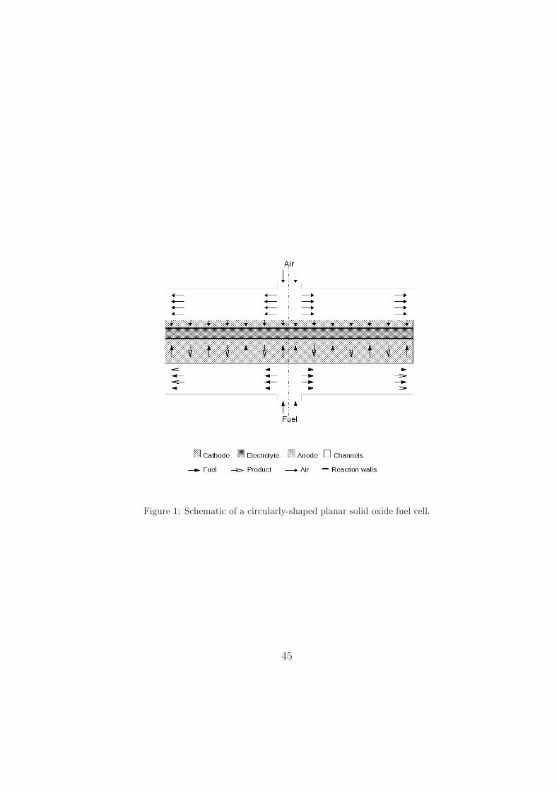
Figure 1: Schematic of a circularly-shaped planar solid oxide fuel cell.

45

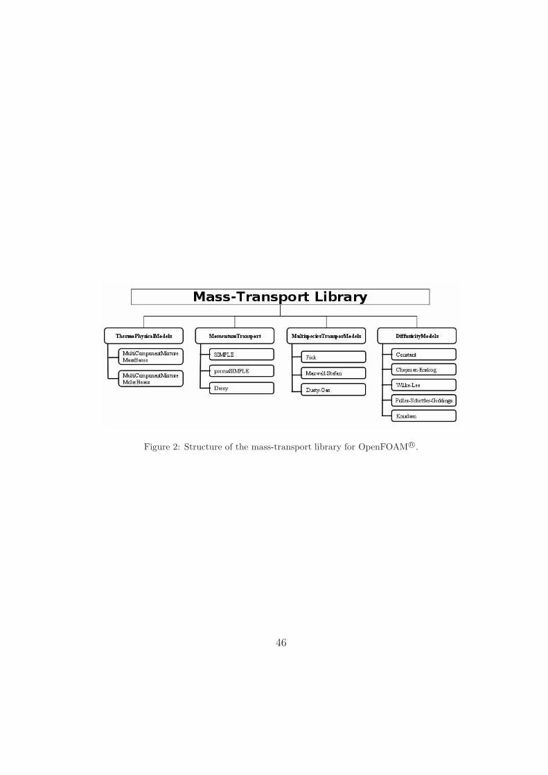
Figure 2: Structure of the mass-transport library for OpenFOAM R©.

46

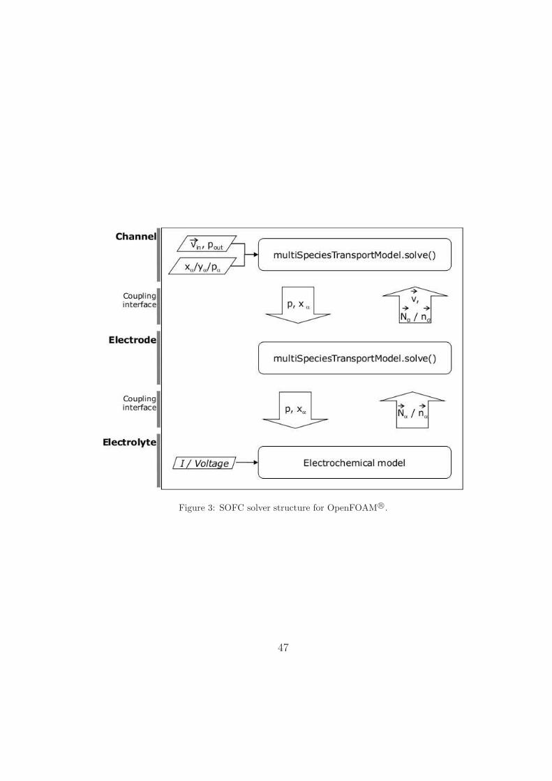
Figure 3: SOFC solver structure for OpenFOAM R©.

47

0

0.2

0.4

0.6

0.8

1

0 0.02 0.04 0.06 0.08 0.1

Mas

s fr

actio

n / -

x / m

Analytical - yH2Analytical - yH2OFick - yH2Fick - yH2O

0

10000

20000

30000

40000

50000

60000

70000

80000

90000

0 0.02 0.04 0.06 0.08 0.1

Par

tial p

ress

ure

/ Pa

x / m

Analytical - pH2Analytical - pH2OAnalytical - pN2Maxwell-Stefan - pH2Maxwell-Stefan - pH2OMaxwell-Stefan - pN2

0

20000

40000

60000

80000

100000

120000

140000

160000

0 0.02 0.04 0.06 0.08 0.1

Par

tial p

ress

ure

/ Pa

x / m

Analytical - pH2Analytical - pH2OAnalytical - pDusty gas - pH2Dusty gas - pH2ODusty gas - p

Figure 4: Mass-transfer library: 1D analytical validation of the FickModel, theMaxwellStefanModel and the DustyGasModel

48

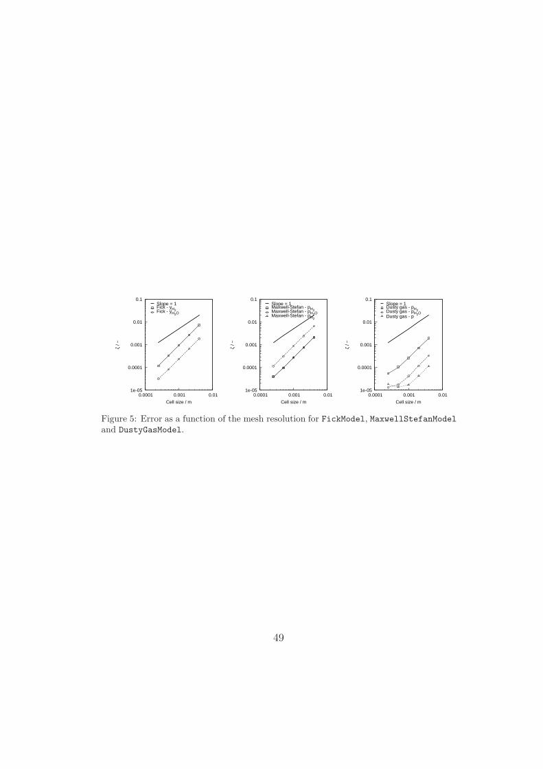
1e-05

0.0001

0.001

0.01

0.1

0.0001 0.001 0.01

ζ / −

Cell size / m

Slope = 1Fick - yH2Fick - yH2O

1e-05

0.0001

0.001

0.01

0.1

0.0001 0.001 0.01

ζ / −

Cell size / m

Slope = 1Maxwell-Stefan - pH2Maxwell-Stefan - pH2OMaxwell-Stefan - pN2

1e-05

0.0001

0.001

0.01

0.1

0.0001 0.001 0.01

ζ / −

Cell size / m

Slope = 1Dusty gas - pH2Dusty gas - pH2ODusty gas - p

Figure 5: Error as a function of the mesh resolution for FickModel, MaxwellStefanModeland DustyGasModel.

49

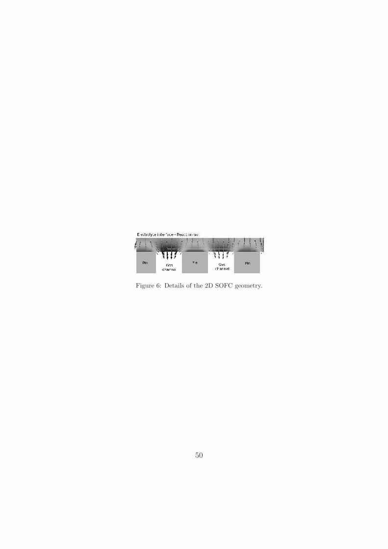
Figure 6: Details of the 2D SOFC geometry.

50

Figure 7: Details of the 3D SOFC geometry

51

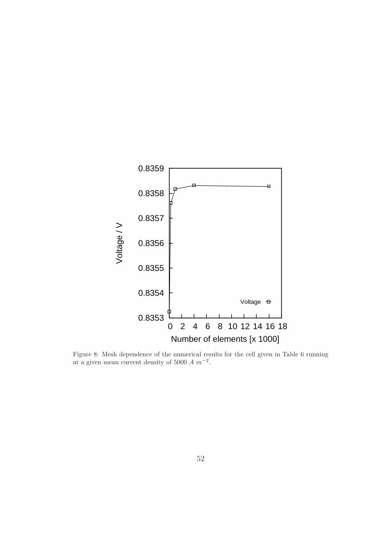
0.8353

0.8354

0.8355

0.8356

0.8357

0.8358

0.8359

0 2 4 6 8 10 12 14 16 18

Vol

tage

/ V

Number of elements [x 1000]

Voltage

Figure 8: Mesh dependence of the numerical results for the cell given in Table 6 runningat a given mean current density of 5000 A m−2.

52

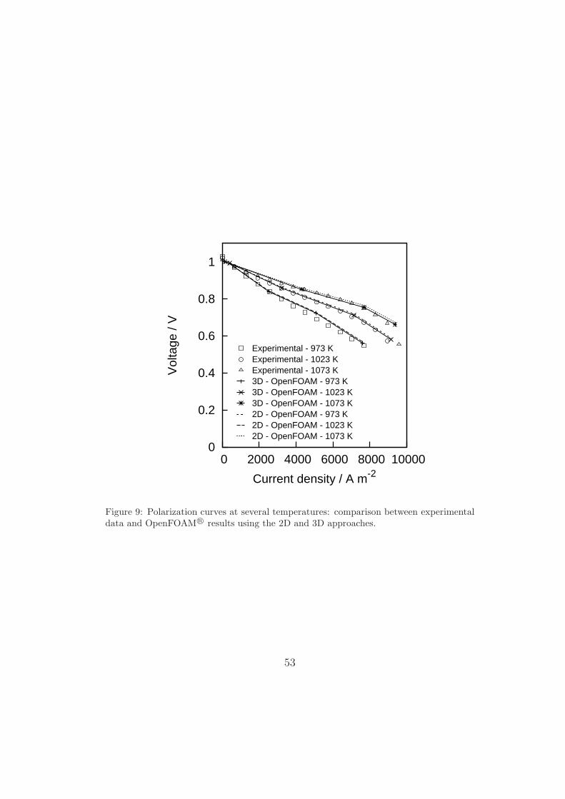
0

0.2

0.4

0.6

0.8

1

0 2000 4000 6000 8000 10000

Vol

tage

/ V

Current density / A m-2

Experimental - 973 KExperimental - 1023 KExperimental - 1073 K3D - OpenFOAM - 973 K3D - OpenFOAM - 1023 K3D - OpenFOAM - 1073 K2D - OpenFOAM - 973 K2D - OpenFOAM - 1023 K2D - OpenFOAM - 1073 K

Figure 9: Polarization curves at several temperatures: comparison between experimentaldata and OpenFOAM R© results using the 2D and 3D approaches.

53

FoamFile

version 2.0;

format ascii;

class volScalarField;

location "0";

object yH2O;

// * * * * * * * * * * * * * * * * * * * * *

dimensions [0 0 0 0 0 0 0];

internalField uniform 0.7;

boundaryField

liquid

type fixedValue;

value uniform 0.7;

exit

type fixedFlux;

gradient uniform 0;

value uniform 0.7;

TreD

type empty;

wall

type zeroGradient;

Figure 10: Initial conditions file for hydrogen mass fraction for Fick validation test case.

54

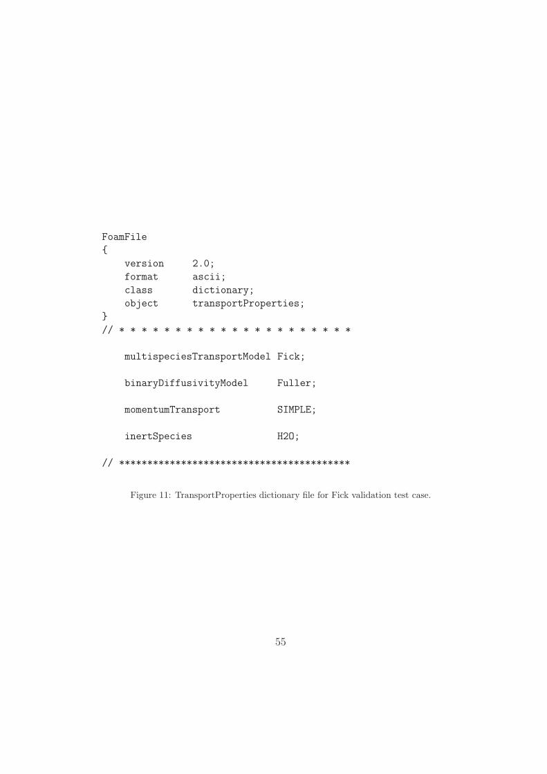
FoamFile

version 2.0;

format ascii;

class dictionary;

object transportProperties;

// * * * * * * * * * * * * * * * * * * * * *

multispeciesTransportModel Fick;

binaryDiffusivityModel Fuller;

momentumTransport SIMPLE;

inertSpecies H2O;

// *****************************************

Figure 11: TransportProperties dictionary file for Fick validation test case.

55

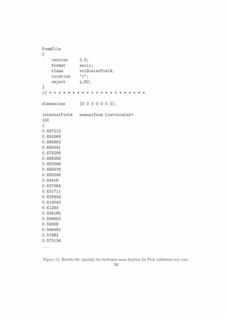
FoamFile

version 2.0;

format ascii;

class volScalarField;

location "1";

object y_H2;

// * * * * * * * * * * * * * * * * * * * * *

dimensions [0 0 0 0 0 0 0];

internalField nonuniform List<scalar>

100

(

0.697212

0.691569

0.685862

0.680091

0.674256

0.668358

0.662398

0.656378

0.650298

0.64416

0.637964

0.631711

0.625404

0.619043

0.61263

0.606165

0.599652

0.59309

0.586482

0.57983

0.573134

...

Figure 12: Results file (partial) for hydrogen mass fraction for Fick validation test case.

56

List of Tables

1 Values of the parameters of the fixedFlux boundary conditionfor the several diffusion models . . . . . . . . . . . . . . . . . 58

2 Boundary conditions required by the SOFC solver . . . . . . . 593 Conditions for the validation of the FickModel for a binary

mixture consisting of H2 and H2O . . . . . . . . . . . . . . . . 604 Conditions for the validation of the MaxwellStefanModel for

a multicomponent mixture consisting of H2, H2O and N2 . . . 615 Conditions for the validation of the DustyGasModel for a bi-

nary mixture consisting of H2, H2O . . . . . . . . . . . . . . . 626 Cell parameters: geometry and operating conditions . . . . . . 63

57

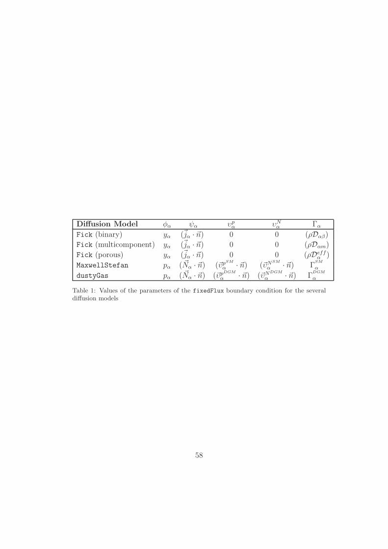
Diffusion Model φα ψα υpα υNα Γα

Fick (binary) yα (~jα · ~n) 0 0 (ρDαβ)

Fick (multicomponent) yα (~jα · ~n) 0 0 (ρDαm)

Fick (porous) yα (~jα · ~n) 0 0 (ρDeffα )

MaxwellStefan pα ( ~Nα · ~n) (~υpSM

α · ~n) (~υNSM

α · ~n) ΓSM

α

dustyGas pα ( ~Nα · ~n) (~υpDGM

α · ~n) (~υNDGM

α · ~n) ΓDGM

α

Table 1: Values of the parameters of the fixedFlux boundary condition for the severaldiffusion models

58

Channel field patch type

Velocity @inlet fixedValue (mass flux)@outlet zeroGradient

@electrode interface fixedValue (from electrode)Pressure @inlet zeroGradient

@outlet fixedValue

@electrode interface zeroGradient

Species concentration @inlet fixedValue (feeding composition)@outlet zeroGradient

@electrode interface fixedFlux (from electrode)Electrode field patch type

Velocity @channel interface zeroGradient@electrolyte interface fixedValue (0 0 0)

Pressure @channel interface fixedValue (from channel)@electrolyte interface zeroGradient

Species concentration @channel interface fixedValue (from channel)@electrolyte interface fixedFlux (Faraday’s Law)

Electrolyte field patch type

Species Concentration @electrode interface fixedValue (from electrode)

Table 2: Boundary conditions required by the SOFC solver

59

Variable Value

Species (α, β) H2, H2OTube length 0.1 mTemperature 1073 KPressure 101325 PayH2(0) 0.7yH2O(0) 0.3nH2(0.1) 5e-4 kg m−2s−1

nH2O(0.1) 0 kg m−2s−1

Dαβ Fuller-Schettler-Giddings

Table 3: Conditions for the validation of the FickModel for a binary mixture consistingof H2 and H2O

60

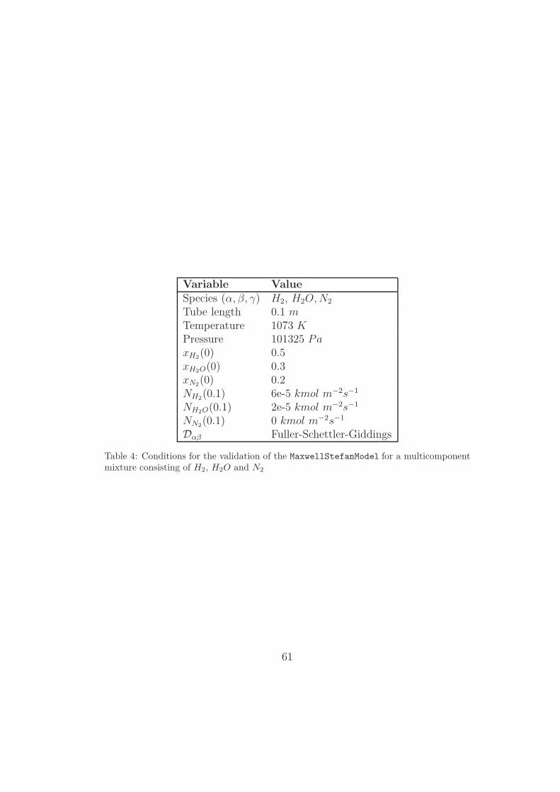
Variable Value

Species (α, β, γ) H2, H2O,N2

Tube length 0.1 mTemperature 1073 KPressure 101325 PaxH2(0) 0.5xH2O(0) 0.3xN2(0) 0.2NH2(0.1) 6e-5 kmol m−2s−1

NH2O(0.1) 2e-5 kmol m−2s−1

NN2(0.1) 0 kmol m−2s−1

Dαβ Fuller-Schettler-Giddings

Table 4: Conditions for the validation of the MaxwellStefanModel for a multicomponentmixture consisting of H2, H2O and N2

61

Variable Value

Species (α, β) H2, H2OTube length 0.1 mTemperature 1073 KPressure 101325 PaxH2(0) 0.7xH2O(0) 0.3NH2(0.1) 5e-6 kmol m−2s−1

NH2O(0.1) -1e-6 kmol m−2s−1

Porosity 0.32Tortuosity 3Pore diameter 1e-6 mDαβ Fuller-Schettler-GiddingsDKα Knudsen

Table 5: Conditions for the validation of the DustyGasModel for a binary mixture consist-ing of H2, H2O

62

Cell Geometry

Cell diameter 78 mmAnode Ni/YSZAnode thickness 520 µmAnode porosity 0.32Anode tortuosity 3Anode permeability 1e-14 520 m2

Cathode LSCFCathode thickness 34 µmCathode porosity 0.32Cathode tortuosity 3Cathode permeability 1e-14 m2

Electrolyte YSZElectrolyte thickness 6 µmActive area 47 cm2

Operating conditions

Pressure 101325 PaTemperature 700, 750, 800 CFuel flow 0.533 Nl min−1

Fuel composition 77 % H2 + 4 % H2O + 19 % N2

Air flow 1.5 Nl min−1

Air composition 21 % O2 + 79 % N2

Table 6: Cell parameters: geometry and operating conditions

63

List of Algorithms

1 Typical implementation of a partial differential equation inOpenFOAMR© . . . . . . . . . . . . . . . . . . . . . . . . . . . 65

2 Structure of the multiSpeciesTransportModel, the segre-gated solver to calculate the species mass-transport . . . . . . 66

64

// Generic equation:

∂ρ~v

∂t+∇ · (ρ~v~v)−∇ · µ (∇~v) = −∇p

// OpenFOAM code:

solve

(

fvm::ddt(rho, U)

+ fvm::div(phi, U)

- fvm::laplacian(mu, U)

==

- fvc::grad(p)

)

Algorithm 1: Typical implementation of a partial differential equation inOpenFOAMR©

65

multiSpeciesTransportModel::solve()

if (Fick or MaxwellStefan)

momentumTransport::momentumLoop()

if (porous)

momentumTransport::porousSIMPLE

else (channels)

momentumTransport::SIMPLE

endif

endif

massTransportLoop()

if (Fick or MaxwellStefan)

for ( α = 1; α < (N − 1); α+ +)speciesEquation.solve() → yα or pαspeciesEquation.flux() → ~nα or ~Nα

endfor

if (Fick)

yN = 1−∑

(α6= N) yα~nN = ρ~v −

∑

(α6= N) ~nα

else (MaxwellStefan)

pN = p− ∑

(α6= N) pα~NN = ρ~vW−1

m− ∑

(α6= N)~Nα

xα = pα / pendif

correct()

calcCoefficients()

else (dustyGas)

for ( α = 1; α < N ; α++)speciesEquation.solve() → pαspeciesEquation.flux() → ~Nα

endfor

p =∑

pαxα = pα / pcorrect()

calcCoefficients()

momentumTransport::Darcy

endif

Algorithm 2: Structure of the multiSpeciesTransportModel, the segre-gated solver to calculate the species mass-transport

66