SAS Enterprise Miner 6.1 Extension Nodes: Developer's Guide

SAS® Enterprise Miner™ 6.1Extension NodesDeveloper’s Guide

TW11117_ColorTitlePage.indd 1 5/20/09 12:30:33 PM

The correct bibliographic citation for this manual is as follows: SAS Institute Inc. 2009.SAS ® Enterprise MinerTM 6.1 Extension Nodes: Developer’s Guide. Cary, NC: SASInstitute Inc.

SAS® Enterprise MinerTM 6.1 Extension Nodes: Developer’s GuideCopyright © 2009, SAS Institute Inc., Cary, NC, USAAll rights reserved. Produced in the United States of America.For a hard-copy book: No part of this publication may be reproduced, stored in aretrieval system, or transmitted, in any form or by any means, electronic, mechanical,photocopying, or otherwise, without the prior written permission of the publisher, SASInstitute Inc.For a Web download or e-book: Your use of this publication shall be governed by theterms established by the vendor at the time you acquire this publication.U.S. Government Restricted Rights Notice. Use, duplication, or disclosure of thissoftware and related documentation by the U.S. government is subject to the Agreementwith SAS Institute and the restrictions set forth in FAR 52.227-19 Commercial ComputerSoftware-Restricted Rights (June 1987).SAS Institute Inc., SAS Campus Drive, Cary, North Carolina 27513.1st electronic book, June 2009SAS® Publishing provides a complete selection of books and electronic products to helpcustomers use SAS software to its fullest potential. For more information about oure-books, e-learning products, CDs, and hard-copy books, visit the SAS Publishing Web siteat support.sas.com/publishing or call 1-800-727-3228.SAS® and all other SAS Institute Inc. product or service names are registered trademarksor trademarks of SAS Institute Inc. in the USA and other countries. ® indicates USAregistration.Other brand and product names are registered trademarks or trademarks of theirrespective companies.

SAS Enterprise Miner 6.1 Extension Nodes: Developer's Guide

Chapter 1: Overview

Chapter 2: Anatomy of an Extension Node

● Icons● XML Properties File● Server Code

Chapter 3: Writing Server Code

● Create Action● Train, Score, and Report Actions● Exceptions● Scoring Code● Modifying Metadata● Results● Model Nodes

Chapter 4: Extension Node Example

Chapter 5: Deploying An Extension Node

Appendix 1: SAS Code Node

Appendix 2: Controls That Require Server Code

Appendix 3: Predictive Modeling

Appendix 4: Allocating Libraries for SAS Enterprise Miner 6.1

Appendix 5: ExtDemo Node

Copyright 2009 by SAS Institute Inc., Cary, NC, USA. All rights reserved.

Chapter 1: Overview Extension nodes provide a mechanism for extending the functionality of a SAS Enterprise Miner installation. Extension nodes can be developed to perform any essential data mining activity (that is, sample, explore, modify, model, or assess [SEMMA]). Although the Enterprise Miner nodes that are distributed by SAS are typically designed to satisfy the needs of a diverse audience, extension nodes provide a means to develop custom solutions.

Developing an extension node is conceptually simple. An extension node consists of the following:

● one or more SAS source code files stored in a SAS library or in external files that are accessible by the Enterprise Miner server

● an XML file defining the properties of the node● two graphic images stored as .gif files.

When properly developed and deployed, an extension node integrates into the Enterprise Miner workspace so that, from the perspective of the end user, it is indistinguishable from any other node in Enterprise Miner. From a developer's perspective, the only difference is the storage location of the files that define an extension node's functionality and appearance. Any valid SAS language program statement can be used in the source code for an extension node, so an extension node's functionality is virtually unlimited.

Although the anatomy of an extension node is fairly simple, the fact that an extension node must function within an Enterprise Miner process flow diagram requires special consideration. An extension node's functionality typically allows for the possibility that the process flow diagram contains predecessor nodes and successor nodes. As a result, your extension node typically includes code designed to capture and process information from predecessor nodes, and to prepare results to pass on to successor nodes. Also, the extension node deployment process involves stopping and restarting the Enterprise Miner server. Because software development is inherently an iterative process, these features introduce obstacles to development not typically encountered in other environments. Fortunately, a solution is readily available: the Enterprise Miner SAS Code node. The SAS Code node provides an ideal environment in which to develop and test your code. You can place a SAS Code node anywhere in a process flow diagram. Using the SAS Code node's Code Editor, you can edit and submit code interactively

while viewing the SAS log and output listings. You can run the process flow diagram path up to and including the SAS Code node and view the Results window without closing the programming interface. Predefined macros and macro variables are readily available to provide easy access to information from predecessor nodes. There are also predefined utility macros that can assist you in generating output for your extension node. In short, you can develop and test your code using a SAS Code node without ever having to actually deploy your extension node.

After you have determined that your server code is robust, you will need to develop and test the XML properties file. The XML properties file is used to populate the extension node's Properties panel, which enables users to set program options for the node's SAS program.

Accessibility Features of SAS Enterprise Miner 6.1 SAS Enterprise Miner 6.1 includes accessibility and compatibility features that improve the usability of the product for users with disabilities. These features are related to accessibility standards for electronic information technology adopted by the U.S. Government under Section 508 of the U.S. Rehabilitation Act of 1973, as amended. SAS Enterprise Miner 6.1 supports Section 508 standards except as noted in the following table.

Section 508 Accessibility Criteria Support Status Explanation

When software is designed to run on a system that has a keyboard, product functions shall be executable from a keyboard where the function itself or the result of performing a function can be discerned textually.

Supported with exceptions.

The software supports keyboard equivalents for all user actions with the following exception:

The Explore action in the data source pop-up menu cannot be invoked directly from the keyboard, but there is an alternative way to invoke the data source explorer using the Variables property in the Properties panel.

Color coding shall not be used as the only means of conveying information, indicating an action, prompting a response, or distinguishing a visual element.

Supported with exceptions.

Node run or failure indication relies on color, but there is always a corresponding message displayed in a pop-up window.

If you have questions or concerns about the accessibility of SAS products, send e-mail to [email protected].

Copyright © 2009 by SAS Institute Inc., Cary, NC, USA. All rights reserved.

Chapter 2: Anatomy of an Extension Node As described in the Overview, an extension node consists of icons, an XML properties file, and a SAS program. To build and deploy an extension node, you must learn the structure of the individual parts as well as how the parts integrate to form a whole. Unfortunately, there is no natural order in which to discuss the individual parts. You cannot learn everything you need to know about one part without first learning something about at least one of the other parts. This chapter provides as complete an introduction to each of the parts as possible without discussing their interdependencies. This chapter also provides the prerequisite knowledge you need to explore the interdependencies in subsequent chapters.

Icons

Each node has two graphical representations. One appears on the SAS Enterprise Miner node Toolbar that is positioned above the process flow diagram. The other graphical representation appears when you drag and drop an icon from the toolbar onto the process flow diagram. The icon that appears on the toolbar requires a 16x16 pixel image and the one that appears in the process flow diagram requires a 32x32 pixel image. Both images should be stored as .gif files. For example, consider the two images here:

When deployed, the 16x16 pixel image appears on the toolbar as follows:

The 32x32 pixel image is used by SAS Enterprise Miner to generate the following icon:

This icon appears on the process flow diagram.

The two .gif files must reside in specific folders on the SAS Enterprise Miner installation's middle-tier server or on the client/server if you are working on a personal workstation installation. The exact path depends on your operating system and where your SAS software is installed, but on all systems the folders are found under the SAS configuration directory. Specifically, the 16x16 image should be stored in the ...\SAS\Config\Levn\analyticsPlatform\apps\EnterpriseMiner\ext\gif16 folder, and the 32x32 image should be stored in the ...\SAS\Config\Levn\analyticsPlatform\apps\EnterpriseMiner\ext\gif32 folder. For example, on a typical Microsoft Windows installation, the full paths are, respectively, as follows:

● C:\SAS\Config\Levn\analyticsPlatform\apps\EnterpriseMiner\ext\gif16● C:\SAS\Config\Levn\analyticsPlatform\apps\EnterpriseMiner\ext\gif32

Both .gif files must have the same filename. Because they are stored in different folders, a name conflict does not arise. You can use any available software to generate the images. The preceding images were generated with Adobe Photoshop Elements 2.0. The 32x32 image was generated first, and then the 16x16 image was created by rescaling the larger image.

XML Properties File

An extension node's XML properties file provides a facility for managing information about the node. The XML file for an extension node is stored under the SAS configuration directory:

...\SAS\Config\Levn\analyticsPlatform\apps\EnterpriseMiner\ext.

The basic structure and minimal features of an XML properties file are as follows:

<?xml version="1.0" encoding="UTF-8"?><!DOCTYPE Component PUBLIC "-//SAS//EnterpriseMiner DTD Components 1.3//EN" "Components.dtd">

<Component type="AF" resource="com.sas.analytics.eminer.visuals.PropertyBundle" serverclass="EM6" name=" " displayName=" " description=" " group=" " icon=" " prefix=" " > <PropertyDescriptors></PropertyDescriptors> <Views></Views>

</Component>

The preceding XML code can be copied verbatim and used as a template for an extension node's XML properties file. XML is case-sensitive, so it is important that the element tags are written as specified in the example. The values for all of the elements' attributes must be quoted strings.

The most basic properties file consists of a single Component element with attributes, a single nested PropertyDescriptors element, and a single nested Views element. In the example properties file depicted here, the PropertyDescriptors and Views elements are empty. As the discussion progresses, the PropertyDescriptors element is populated with a variety of Property elements and Control elements; the Views element is populated with a variety of View elements, Group elements, and PropertyRef elements. Some of these elements are used to integrate the node into the SAS Enterprise Miner application. Some elements link the node with a SAS program that you write to provide the node with computational functionality. Other elements are used to populate the node's Properties panel, which serves as a graphical user interface (GUI) for the node's SAS program.

Component Element

The Component element encompasses all other elements in the properties file. The attributes of the Component element provide information that is used to integrate the extension node into the SAS Enterprise Miner environment. All extension nodes share three common Component attributes: type, resource, and serverclass. These three attributes must have the values that are displayed in the preceding example. The values of the other Component attributes are unique for each extension node. These other Component attributes convey the following information:

● name — the name of the node as it appears on the node's icon in a process flow diagram.● displayName — the name of the node that is displayed in the tooltip for the node's icon on the node Toolbar and in the

tooltip for the node's icon in a process flow diagram. The amount of text that can be displayed on an icon is limited but tooltips can accommodate longer strings.

● description — a short description of the node that appears as a tooltip for the node Toolbar.● group — the SEMMA group where the node appears on the SAS Enterprise Miner node Toolbar. The existing SEMMA

group values are as follows:

�❍ SAMPLE�❍ EXPLORE�❍ MODIFY�❍ MODEL�❍ ASSESS�❍ UTILITY

If you select a value from this list, your extension node's icon appears on the toolbar under that group. However, you can add your own group to the SEMMA toolbar by specifying a value that is not in this list.

● icon — the name of the two .gif files that are used to generate the SAS Enterprise Miner icons. The two .gif files share a common filename.

● prefix — a string used to name files (data sets, catalog, and so on) that are created on the server. The prefix must be a valid SAS variable name and should be as short as possible. SAS filenames are limited to 32 characters, so if your prefix is k characters long, SAS Enterprise Miner is left with 32-k characters with which to name files. The shorter the prefix, the greater the flexibility the application has for generating unique filenames.

Consider the following example:


<Component type="AF" resource="com.sas.analytics.eminer.visuals.PropertyBundle" serverclass="EM6" name="Example" displayName="Example" description="Extension Node Example" group="EXPLORE" icon="Example.gif" prefix="EXMPL" >

<PropertyDescriptors></PropertyDescriptors>

<Views></Views>

</Component>

The displayName="Example" and description="Extension Node Example" attributes together produce the tooltip that appears when you hover your mouse over the extension node's icon on the node Toolbar.

The name="Example" attribute produces the name on the icon in the following example. The displayName="Example" produces the tooltip that is displayed when you hover your mouse over the node's icon in the process flow diagram.

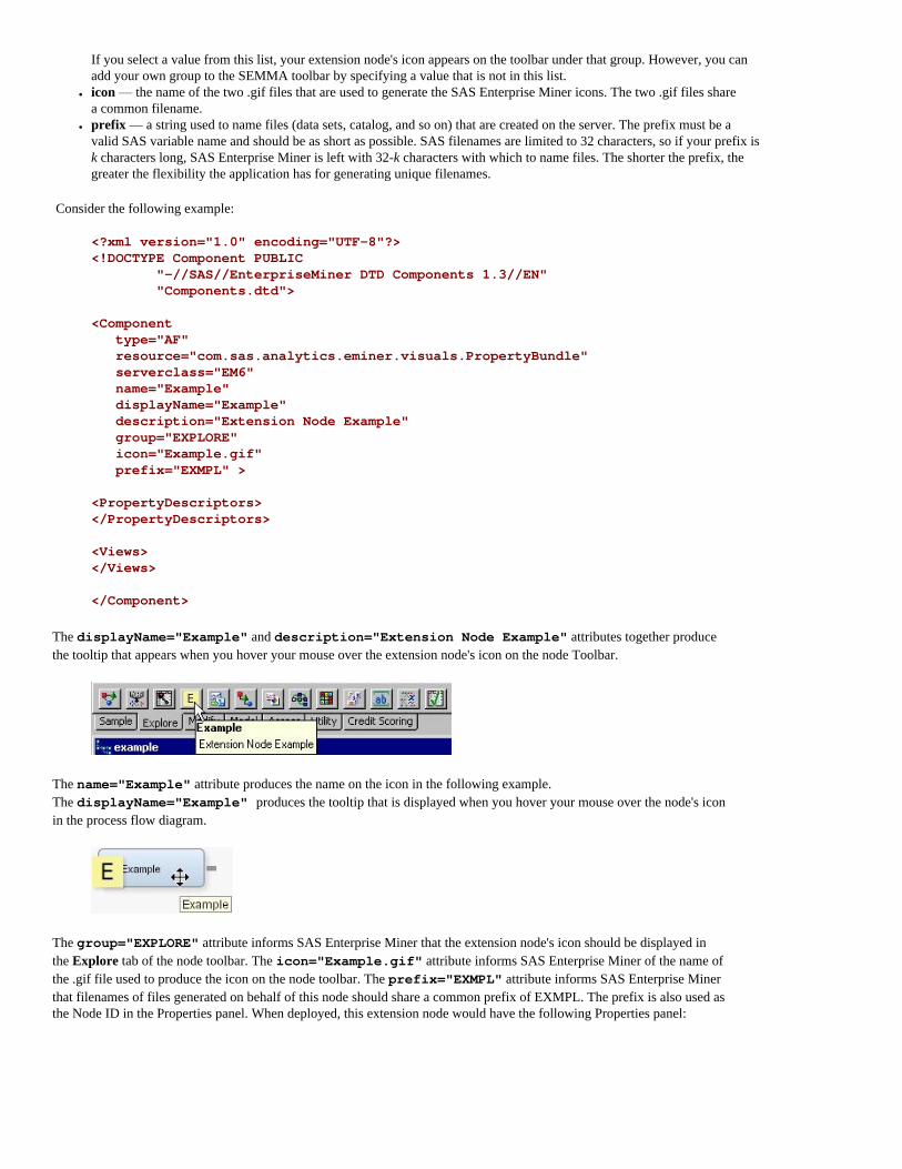
The group="EXPLORE" attribute informs SAS Enterprise Miner that the extension node's icon should be displayed in the Explore tab of the node toolbar. The icon="Example.gif" attribute informs SAS Enterprise Miner of the name of the .gif file used to produce the icon on the node toolbar. The prefix="EXMPL" attribute informs SAS Enterprise Miner that filenames of files generated on behalf of this node should share a common prefix of EXMPL. The prefix is also used as the Node ID in the Properties panel. When deployed, this extension node would have the following Properties panel:

The General properties and Status properties that are displayed here are common to all nodes and are generated automatically by SAS Enterprise Miner.

PropertyDescriptors Element

The PropertyDescriptors element provides structure to the XML document. Having all of the Property elements encompassed by a single PropertyDescriptors element isolates the Property elements from the rest of the file's contents and promotes efficient parsing. The real information content of the PropertyDescriptors element is provided by the individual Property elements that you place within the PropertyDescriptors element. A variety of Property elements can be used in an extension node. Each type of Property element is discussed in detail here. Working examples for each type of Property element are also provided.

Property Elements

The different types of Property elements are distinguished by their attributes. The attributes that are currently supported for extension nodes are as follows:

● type — specifies one of four supported types of Property element. The supported types are as follows:

�❍ String �❍ boolean �❍ int �❍ double

These values are case-sensitive.

● name — a name by which the Property element is referenced elsewhere in the properties file and in the node's SAS code. At run time, SAS Enterprise Miner generates a corresponding macro variable with the name &EM_PROPERTY_name. By default, &EM_PROPERTY_name resolves to the value that is declared in the initial attribute of the Property element. If a user specifies a value for the property in the Properties panel, &EM_PROPERTY_name resolves to that new value. Macro variable names are limited to 32 characters. Twelve characters are reserved for the EM_PROPERTY_ prefix, so the value specified for the name attribute must be 20 characters or less.

● displayName — the name of the Property element that is displayed in the node's Properties panel.● description — the description of the Property element that is displayed in the node's Properties panel.● initial — defines the initial or default value for the property.● edit — indicates whether the user can modify the property's value. Valid values are Y and N.

Some Property elements support all of these attributes, and some support only a subset.

Examples of the syntax for each of the four types of Property elements are provided here. These examples can be copied and used to create your own properties file. All you need to do is change the values for the name, displayName, description, initial, and edit attributes.

String Property

<Property

type="String" name="StringExample" displayName="String Property Example" description="write your own description here" initial="Initial Value" edit="Y" />

The value of a String Property is displayed as a text box that a user can edit. Use a String Property when you want the user to type in a string value. For example, your extension node might create a new variable, and you could allow the user to provide a variable label.

Location and Catalog Properties

The preceding example is typical of a String Property element that corresponds to a specific option or argument of the node's SAS program. However, there are two special String Property elements, referred to as the Location Property and the Catalog Property, that you must include in the properties file. These two special String Property elements are used to inform SAS Enterprise Miner of the location of the node's SAS program. These two Property elements appear as follows:

<Property type="String" name="Location" initial="CATALOG"/> <Property type="String" name = "Catalog" initial="SASHELP.EMEXT.Example.SOURCE"/>

The Location Property should be copied verbatim. The Catalog Property can also be copied. However, you should change the value of the initial attribute to the name of the file that contains the entry point of your SAS program in the Catalog Property. As discussed later in the section on Server Code, your SAS program can be stored in several separate files. However, there must always be one file that contains a main program that executes first. The value of the initial attribute of the Catalog Property should be set to the name of this file. If you want to store the main program in an external file, you still need to create a source file that is stored in a SAS catalog. The contents of that file would then simply have the following form:

filename temp 'file-name'; %include temp; filename temp;

Here, file-name is the name of the external file containing the main program.

Boolean Property

<Property type="boolean" name="BooleanExample" displayName="Boolean Property Example" description="write your own description here" initial="Y" />

The Boolean Property is displayed as a drop-down list; the user can select either Yes or No.

Integer Property

<Property type="int" name="Integer" displayName="Integer Property Example"

description="write your own description here" initial="20" edit="Y"></Property>

The value of an Integer Property is displayed as a text box that a user can edit. Use an Integer Property when you want the user to provide an integer value as an argument to your extension node's SAS program.

Double Property

<Property type="double" name="Double" displayName="Double Property Example" description="write your own description here" initial="0.02" edit="Y"></Property>

The value of a Double Property is displayed as a text box that a user can edit. Use a Double Property when you want the user to provide a real number as an argument to your extension node's SAS program.

Properties of these types appear as depicted in the following Properties panel:

These are the most basic forms of the available Property elements. For some applications, these basic forms are sufficient. In many cases, however, you might want to provide a more sophisticated interface. You might also want to restrict the set of valid values that a user can enter. Such added capability is provided by Control elements.

Note: For this example, all of the newly created properties were placed under the heading Train. That heading was generated using a View element discussed later.

Control Elements

In addition to specifying the attributes for a Property element, you can also specify one of several types of Control elements. Control elements are nested within Property elements. Seven types of Control elements are currently supported for extension nodes. Each type of Control element has its own unique syntax. The seven types of Control elements are listed here:

● ChoiceList — displays a predetermined list of values.● Range — validates a numeric value entered by the user.

● SASTABLE — opens a Select a SAS Table window enabling the user to select a SAS data set.● FileTransfer — provides a dialog box enabling a user to select a registered model.● Dialog — opens a dialog box providing access to a variables table from a predecessor data source node, an external text file,

or a SAS data set.● TableEditor — displays a table and permits the user to edit the columns of the table.● DynamicChoiceList — displays a dynamically generated list of values. This type of Control element is used with

a TableEditor Control element.

Some Control elements require accompanying server code to provide functionality. These include the TableEditor, DynamicChoiceList, Filetransfer, and some Dialog Control elements. Examples of these types of Control elements are presented in a later chapter following a discussion of extension node server code.

Examples of the syntax for each of the four types of Control elements that do not require server code follow. These examples can be copied and used to create your own properties file.

String Property with a ChoiceList Control

<Property type="String" name="ChoiceListExample" displayName="Choice List Control Example" description="write your own description here" initial="SEGMENT"> <Control> <ChoiceList> <Choice rawValue="SEGMENT" displayValue="Segment" /> <Choice rawValue="ID" displayValue="ID" /> <Choice rawValue="INPUT" displayValue="Input" /> <Choice rawValue="TARGET" displayValue="Target" /> </ChoiceList> </Control></Property>

A ChoiceList Control enables you to present the user with a drop-down list containing predetermined values for a property. A String Property with a ChoiceList Control consists of the following items:

● a Property element with attributes.● a single Control element.● a single ChoiceList element.● two or more Choice elements. Each Choice element represents one valid value for a program option or argument.

Each Choice element has the following attributes:

● rawValue — the value that is passed to the node's SAS program.● displayValue — the value that is displayed to the user in the Properties panel. It can be any character string. If no

displayValue is provided, the rawValue is displayed.

Note: Make sure that the value of the initial attribute of the Property element matches the rawValue attribute of one of the Choice elements. The value of the Property element's initial attribute is the default value for the property; it is the value that is passed to your SAS program if the user doesn't select a value from the Properties panel. If the initial attribute does not match the rawValue attribute of one of the Choice elements, you could potentially be passing an invalid value to your SAS program. To avoid case mismatches, it is a good practice to write the rawValue attributes and the initial attribute using all capital letters.

String Property with a Dialog Control

There are three types of Dialog Control elements supported for extension nodes in Enterprise Miner 6.1. The Dialog elements are uniquely distinguished by their class attributes. The class attributes are as follows:

● com.sas.analytics.eminer.visuals.VariablesDialog● com.sas.analytics.eminer.visuals.CodeNodeScoreCodeEditor● com.sas.analytics.eminer.visuals.InteractionsEditorDialog

In each of the three cases, the class attribute must be specified verbatim. The Dialog Control with class=com.sas.analytics.eminer.visuals.VariablesDialog is the only Dialog Control of the three that does not require accompanying server code.

Dialog Control with class=com.sas.analytics.eminer.visuals.VariablesDialog

<Property type="String" name="VariableSet" displayName="Variables" description="Variable Properties"> <Control> <Dialog class="com.sas.analytics.eminer.visuals.VariablesDialog" showValue="N" /> </Control></Property>

This Property element configuration provides access to the variables exported by a predecessor Data Source node. Notice the class attribute of the Dialog element. When you include a Property element of this type, the displayName value is displayed in the Properties panel and an ellipsis icon ( ) is displayed in the Value column.

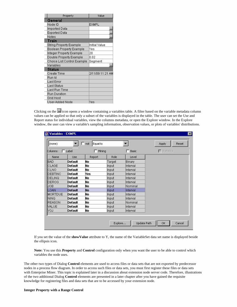
Clicking on the icon opens a window containing a variables table. A filter based on the variable metadata column values can be applied so that only a subset of the variables is displayed in the table. The user can set the Use and Report status for individual variables, view the columns metadata, or open the Explore window. In the Explore window, the user can view a variable's sampling information, observation values, or plots of variables' distributions.

If you set the value of the showValue attribute to Y, the name of the VariableSet data set name is displayed beside the ellipsis icon.

Note: You use this Property and Control configuration only when you want the user to be able to control which variables the node uses.

The other two types of Dialog Control elements are used to access files or data sets that are not exported by predecessor nodes in a process flow diagram. In order to access such files or data sets, you must first register these files or data sets with Enterprise Miner. This topic is explained later in a discussion about extension node server code. Therefore, illustrations of the two additional Dialog Control elements are presented in a later chapter after you have gained the requisite knowledge for registering files and data sets that are to be accessed by your extension node.

Integer Property with a Range Control

<Property type="int" name="Range" displayName="Integer Property with Range Control" description="write your own description here" initial="20" edit="Y"> <Control> <Range min="1" excludeMin="N" max="1000" excludeMax="N"/> </Control></Property>

The addition of the Range Control element to an Integer Property element enables you to restrict the range of permissible values that a user can enter. The Control element has no attributes in this case. Instead, a Range element is nested within the Control element. The Range element has these four attributes:

● min — an integer that represents the minimum of the range of permissible values.● excludeMin — when this attribute is set to Y, the minimum value of the range that is declared in the min attribute is

excluded as a permissible value. When this attribute is set to N, the minimum value is a permitted value.● max — an integer that represents the maximum of the range of permissible values.● excludeMax — when this attribute is set to Y, the maximum value of the range that is declared in the max attribute is

excluded as a permissible value. When this attribute is set to N, the maximum value is a permitted value.

If the user enters a value that is outside the permissible range, the value reverts to the previous valid value.

Double Property with a Range Control

<Property type="double" name="double_range" displayName="Double Property with Range Control" description="write your own description here" initial="0.33" edit="Y"> <Control> <Range min="0" excludeMin="Y" max="1" excludeMax="Y" /> </Control></Property>

The addition of the Range Control element to a Double Property element enables you to restrict the range of permissible values that a user can enter. The Control element has no attributes in this case. Instead, a Range element is nested within the Control element. The Range element has these four attributes:

● min — a real number that represents the minimum of the range of permissible values.● excludeMin — when this attribute is set to Y, the minimum value of the range that is declared in the min attribute is

excluded as a permissible value. When this attribute is set to N, the minimum value is a permitted value.● max — a real number that represents the maximum of the range of permissible values.● excludeMax — when this attribute is set to Y, the maximum value of the range that is declared in the max attribute is

excluded as a permissible value. When this attribute is set to N, the maximum value is a permitted value.

If the user enters a value that is outside the permissible range, the value reverts to the previous valid value.

String Property with a SASTABLE Control

<Property type="String"

name="SASTable" displayName="SASTABLE Control Example" description="write your own description here" initial="" edit="Y"> <Control type="SASTABLE" showValue="Y" showSystemLibraries="Y" noDataSpecified="Y" /></Property>

A SASTABLE Control element enables the user to select the name of a SAS data set. The default value of a String Property element with a SASTABLE Control is a null string.

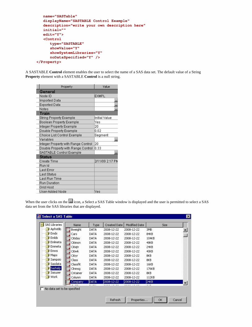
When the user clicks on the icon, a Select a SAS Table window is displayed and the user is permitted to select a SAS data set from the SAS libraries that are displayed.

This Control element has these four attributes:

● type — declares the type of control. This attribute value must be set to "SASTABLE" to produce the effect depicted here.● showValue — when set to Y, this attribute displays the name of the data set selected by the user in the Value column of the

Properties panel. When this attribute is set to N, the Value column of the Properties panel remains empty even when a user has selected a data set.

● showSystemLibraries — when this attribute is set to Y, SAS Enterprise Miner project libraries are displayed in the Select a SAS Table window. When this attribute is set to N, SAS Enterprise Miner project libraries are not displayed in the Select a SAS Table window. For example, in the previous example, notice the SAS Enterprise Miner project libraries Emds, Emlds, Emlmeta, Emmeta, and Emws2. If the showSystemLibraries attribute had been set to N, these SAS Enterprise Miner libraries would not be displayed.

● noDataSpecified — When this attribute is set to Y, a check box with the label "No data set to be specified" appears in the bottom left corner of the Select a SAS Table window. When checked, the SASTABLE Control is cleared and the value of the String Property is set to null. When set to N, this attribute has no effect.

The default values of the property and the corresponding macro variable &EM_PROPERTY_propertyname are null. When a user selects a data set, the name of the data set is assigned to &EM_PROPERTY_propertyname and is displayed in the Value column of the Properties panel. The property's value can be changed to another data set name by clicking on the icon and selecting a new data set. Clicking on the icon and then clicking on the No data set to be specified check box clears the property.

String Property with a TableEditor Control: A Preview

A String Property with a TableEditor Control requires SAS code in order for it to function properly. Because this Control requires server code, which has not yet been discussed, a complete discussion and example of this type of Property and Control configuration is provided in Appendix 2: Controls That Require Server Code. This section provides a preview of the most basic type of table editor. This preview also serves as a reference example for the discussion on server code in the next chapter.

When a String Property with a TableEditor Control is implemented, an ellipsis icon ( ) appears in the Value column of the Properties panel next to the Property name.

Clicking on the icon opens a Table Editor window, which displays a table that is associated with the Control element.

Depending on how the Control element is configured, a user might then edit some or all of the values in the table. You also have the option of writing specially identified blocks of SAS code that execute either when the table first opens or when the table is closed.

Views

The Views element organizes properties in the Properties panel. The following Properties panel contains one of each type of Property element:

Here is the Views element of the XML properties file that generates this Properties panel:

<Views> <View name="Train"> <PropertyRef nameref="StringExample"/> <PropertyRef nameref="BooleanExample"/> <PropertyRef nameref="Integer"/> <PropertyRef nameref="Double"/> <PropertyRef nameref="ChoiceListExample"/> <PropertyRef nameref="VariableSet"/> <PropertyRef nameref="Range"/> <PropertyRef nameref="double_range"/> <PropertyRef nameref="SASTable"/> </View></Views>

Within the Views element, there is a single View element. That View element has a single attribute — name — and its value is Train. Nested within the View element is a collection of PropertyRef elements. There is one PropertyRef element for each Property element in the properties file. Each PropertyRef element has a single nameref attribute. Each nameref has a value that corresponds to the name attribute of one of the Property elements.

When you add the Train View element, SAS Enterprise Miner separates the node's properties into three groups: General, Train, and Status. The General and Status groups are automatically generated and populated by SAS Enterprise Miner. These two groups and the properties that populate them are common to all nodes and do not have to be specified in the extension node's XML properties file. The Train group contains all of the properties that are specified by the PropertyRef elements that are nested within the Train View element.

Now suppose that instead of a single View element, there were three View elements: Train, Score, and Report. Suppose that we also remove some of the PropertyRef elements from the Train View, put some in the Score View, and put the rest in the Report View, as follows:

<Views> <View name="Train"> <PropertyRef nameref="StringExample"/> <PropertyRef nameref="BooleanExample"/> <PropertyRef nameref="Integer"/> <PropertyRef nameref="Double"/> </View> <View name="Score">

<PropertyRef nameref="ChoiceListExample"/> <PropertyRef nameref="VariableSet"/> <PropertyRef nameref="SASTable"/> </View> <View name="Report"> <PropertyRef nameref="Range"/> <PropertyRef nameref="double_range"/> </View></Views>

The following Properties panel would appear as a result:

By convention, SAS Enterprise Miner nodes use only three View elements with the names Train, Score, and Report. However, not all nodes need all three View elements. Although it is recommended, you are not required to follow this convention. Your node can have as many different View elements as you like and you can use any names that you want for the View elements.

Group Elements

You can indicate to the user when a set of Property elements is related by placing the related Property elements in a group. When a group is defined, all of the properties in the group appear as items in an expandable and collapsible list under a separate subheading. This is accomplished by nesting a Group element within a View element and then nesting PropertyRef elements inside of the Group element.

Group elements have two attributes:

● name — uniquely identifies the Group to the Enterprise Miner server.● displayName — the name of the Group that is displayed in the node's Properties panel.● description — the description of the Group that is displayed in the node's Properties panel.

For example, consider the following Views configuration:

<Views> <View name="Train"> <PropertyRef nameref="StringExample" /> <PropertyRef nameref="BooleanExample" /> <Group

name="GroupExample" displayName="Group Example" description="write your own description here"> <PropertyRef nameref="Integer" /> <PropertyRef nameref="Double" /> <PropertyRef nameref="ChoiceListExample" /> </Group> <PropertyRef nameref="VariableSet" /> <PropertyRef nameref="SASTable" /> <PropertyRef nameref="Range" /> <PropertyRef nameref="double_range" /> </View></Views>

The following Properties panel results:

You can click on the + or - sign beside the Group name to expand or collapse, respectively, the list of properties that are included in a group.

You can examine the XML properties files of existing SAS Enterprise Miner nodes and use them as guides to constructing your own properties files. The exact location of these files depends upon your operating system and installation configuration, but they can be found under the SAS configuration directory:

...\SAS\Config\Lev1\AnalyticsPlatform\apps\EnterpriseMiner\conf\components

Be aware, however, that SAS Enterprise Miner nodes can have features that are not supported for extension nodes. If you see an attribute in a SAS node's XML properties file that is not documented here, assume that the attribute is not supported for extension nodes.

SubGroup Elements

You might also encounter situations where your node's SAS program has many options and arguments. In such cases, the list of properties can become too long to conveniently display in the Properties panel. In such situations, you might want to

have related properties in their own separate Properties panel. This is accomplished by using SubGroup elements. SubGroup elements have essentially the same structure as Group elements. That is, SubGroup elements have these three attributes:

● name — uniquely identifies the SubGroup to the Enterprise Miner server.● displayName — the name of the SubGroup that is displayed in the node's Properties panel.● description — the description of the SubGroup that is displayed in the node's Properties panel.

Nest the SubGroup element within a View element, and nest PropertyRef elements within the SubGroup element. When a SubGroup element is used, an icon appears in the Value column of the Properties panel next to the displayName of the SubGroup. Clicking the icon opens a child window. The properties that are nested within the SubGroup element are displayed in that window. The Property elements and Control elements within the SubGroup's Properties panel function the same way that they function in the main Properties panel.

For example, consider the following Views element:

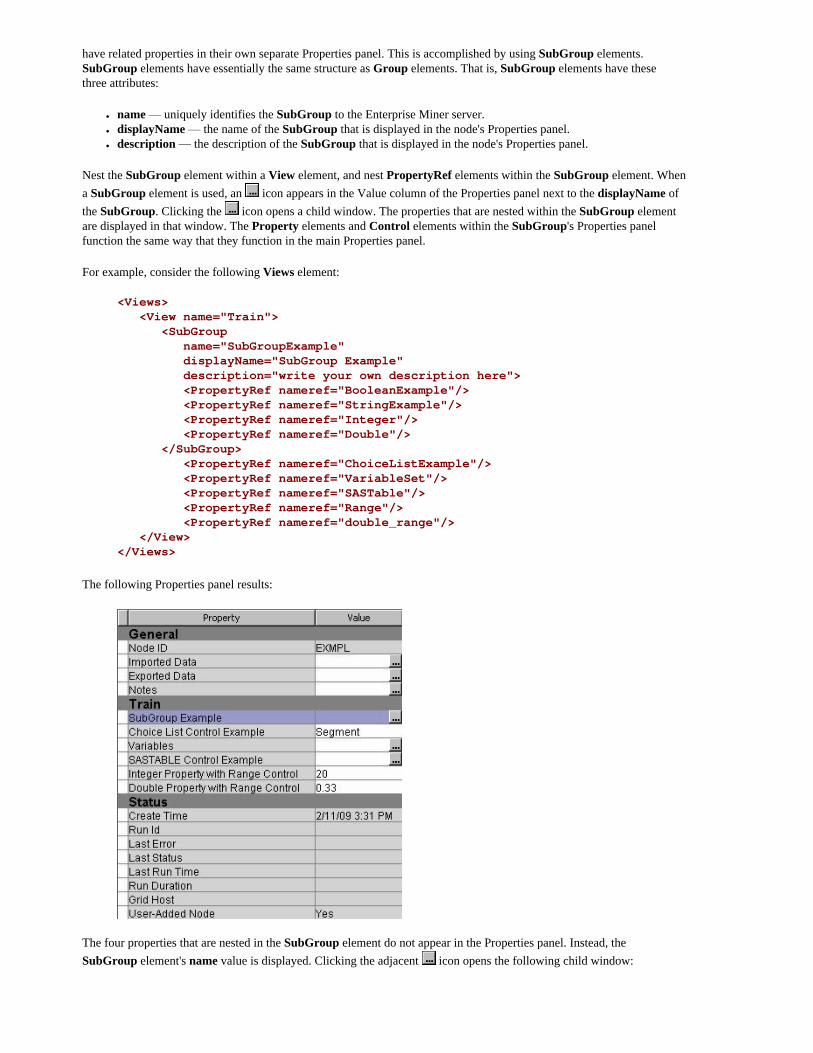
<Views> <View name="Train"> <SubGroup name="SubGroupExample" displayName="SubGroup Example" description="write your own description here"> <PropertyRef nameref="BooleanExample"/> <PropertyRef nameref="StringExample"/> <PropertyRef nameref="Integer"/> <PropertyRef nameref="Double"/> </SubGroup> <PropertyRef nameref="ChoiceListExample"/> <PropertyRef nameref="VariableSet"/> <PropertyRef nameref="SASTable"/> <PropertyRef nameref="Range"/> <PropertyRef nameref="double_range"/> </View></Views>

The following Properties panel results:

The four properties that are nested in the SubGroup element do not appear in the Properties panel. Instead, the SubGroup element's name value is displayed. Clicking the adjacent icon opens the following child window:

Server Code

The specific function of each node is performed by a SAS program that is associated with the node. Thus, when a node is placed in a process flow diagram, it is a graphical representation of a SAS program. An extension node's SAS program consists of one or more SAS source code files residing on the SAS Enterprise Miner server. The source code can be stored in a SAS library or in external files. Any valid SAS statement can be used in an extension node's SAS program. However, you cannot issue statements that generate a SAS windowing environment. The SAS windowing environment from Base SAS is not compatible with SAS Enterprise Miner. For example, you cannot execute SAS/LAB software from within an extension node. As you begin to design your node's SAS program, ask yourself these five questions:

● What needs to occur when the extension node's icon is initially placed in a process flow diagram? ● What is the node going to accomplish at run time? ● Will the node generate Publish or Flow code? ● What types of reports should be displayed in the node's Results window? ● What program options or arguments should the user be able to modify; what should the default values be; and should

the choices, or range of values, be restricted?

SAS Enterprise Miner 5.3 introduced two new features that can significantly enhance the performance of extension nodes: the EM6 server class and the &EM_ACTION macro variable. With these features, a node's code can be separated into the following actions that identify the type of code that is running:

● CREATE — executes only when the node is first placed on a process flow diagram.

● TRAIN — executes the first time the node is run. Subsequently, it executes when one of the following occurs:

�❍ A user runs the node and an input data set has changed.�❍ A user runs the node and the variables table has changed.�❍ A user runs the node and one of the node's Train properties has been changed.

● SCORE — executes the first time the node is run. Subsequently, it executes when one of the following occurs:

�❍ A user runs the node and an input data set has changed.�❍ A user runs the node and one of the node's Score properties has been changed.�❍ The TRAIN action has executed.

● REPORT — executes the first time the node is run. Subsequently, it executes when one of the following occurs:

�❍ A user runs a node and one of the node's Report properties has been changed.�❍ The TRAIN or SCORE action has executed.

To take advantage of this feature, write your code as separate SAS macros. SAS Enterprise Miner executes the macros sequentially, each triggered by an internally generated &EM_ACTION macro variable. That is, the &EM_ACTION macro variable initially resolves to a value of CREATE. When all code associated with that action has completed, the &EM_ACTION macro variable is updated to a value of TRAIN. When all code associated with the TRAIN action has executed, the &EM_ACTION macro variable is updated to a value of SCORE. After all code

associated with the SCORE action has executed, the &EM_ACTION macro variable is updated to a value of REPORT; all code associated with the REPORT action is then executed.

Each Property that you define in the node's XML properties file can be assigned an action value. When a node is placed in a process flow diagram and the process flow diagram is run initially, all of the node's code executes and all executed actions are recorded. When the process flow diagram is run subsequently, the code doesn't have to execute again unless a property setting, the variables table, or data imported from a predecessor node has changed. If a user has changed a property setting, SAS Enterprise Miner can determine what action is associated with that property. Thus, it can begin the new execution sequence with that action value. For example, suppose that a user changes a REPORT property setting. The TRAIN and SCORE code does not have to execute again. This can save significant computing time, particularly when you have large data sets, complex algorithms, or many nodes in a process flow diagram.

You are not required to take advantage of actions, and your code is not required to conform to any particular structure. However, to take full advantage of the actions mechanism, write your SAS code so that it conforms to the following structure:

%macro main;

%if %upcase(&EM_ACTION) = CREATE %then %do;

/*add CREATE code */

%else;

%if %upcase(&EM_ACTION) = TRAIN %then %do;

/*add TRAIN code */

%else;

%if %upcase(&EM_ACTION) = SCORE %then %do;

/*add SCORE code */

%else;

%if %upcase(&EM_ACTION) = REPORT %then %do;

/*add REPORT code */

%mend main;

%main;

Typically, the code associated with the CREATE, TRAIN, SCORE, and REPORT actions consists of four separate macros — %Create, %Train, %Score, and %Report.

All nodes do not have code associated with all four actions. This poses no problem. SAS Enterprise Miner recognizes only the entry point that you declare in the node's XML properties file. It initializes the &EM_ACTION macro variable and submits the main program. If the main program does not include any code that is triggered by a particular action, the &EM_ACTION macro variable is updated to the next action in the sequence. Therefore, if you do not separate your code by actions, all code is treated like TRAIN code; the entire main program must execute completely every time the node is run.

A common practice used for SAS Enterprise Miner nodes is to place the macro, %Main, in a separate file named name.source. name is the name of the node and typically corresponds to the value of the name attribute of the Components element in the XML properties file. name.source serves as the entry point for the extension node's SAS program. It is also common practice to place the source code for the %Create, %Train, %Score, and %Report macros in separate files with names like name_create.source, name_train.source, name_score.source, and name_report.source. There might also be additional files containing other macros or actions with names like name_macros.source and name_actions.source (these types of actions are discussed in Appendix 2: Controls That Require Server Code. To implement this strategy, use FILENAME and %INCLUDE statements in the %Main macro to access the other files. For example, assume that your extension node's SAS program is stored in the Sashelp library in a SAS catalog named Sashelp.Emext and that the catalog contains these five files:

● example.source● example_create.source● example_train.source● example_score.source● example_report.source

Example.source would contain the %Main macro, and it would appear as follows:

/* example.source */ %macro main; %if %upcase(&EM_ACTION) = CREATE %then %do;

filename temp catalog 'sashelp.emext.example_create.source'; %include temp; filename temp; %create; %end;

%else %if %upcase(&EM_ACTION) = TRAIN %then %do;

filename temp catalog 'sashelp.emext.example_train.source'; %include temp; filename temp; %train;

%end;

%else %if %upcase(&EM_ACTION) = SCORE %then %do;

filename temp catalog 'sashelp.emext.example_score.source'; %include temp; filename temp; %score; %end;

%else %if %upcase(&EM_ACTION) = REPORT %then %do;

filename temp catalog 'sashelp.emext.example_report.source'; %include temp; filename temp; %report; %end;

%mend main;

%main;

The other four files would contain their respective macros. There is more to this strategy than simple organizational efficiency; it can actually enhance performance. To illustrate, consider the following scenario. When a node is first placed in a process flow diagram, the entire main program is read and processed. Suppose your TRAIN code contains a thousand lines of code. If the code is contained in the main program, all thousand lines of TRAIN code must be read and processed. However, if the TRAIN code is in a separate file, that code is not processed until the first time the node is run.

A similar situation can occur at run time. At run time, the entire main program is processed. Suppose the node has already

been run once and the user has changed a Report property. The actions mechanism prevents the TRAIN code from executing again. However, if your TRAIN code is stored in a separate file, the TRAIN code does not have to be read and processed. This is the recommended strategy.

To store your code in external files rather than in a SAS catalog, simply alter the FILENAME statements accordingly. However, you must store the entry point file (for example, example.source) in a catalog and place it in a SAS library that is accessible by Enterprise Miner. The simplest way to do this is to include your catalog in the Sashelp library by placing the catalog in the SASCFG folder. The exact location of this folder depends on your operating system and your installation configuration, but it is always found under the root SAS directory and has a path resembling ...\SAS\SASFoundation\9.2\nls\en\SASCFG. For example, on a typical Windows installation, the path is as follows:

C:\Program Files\SAS\SASFoundation\9.2\nls\en\SASCFG.

You can also store the catalog in another folder and then modify the SAS system configuration file Sasv9.cfg so that this folder is included in the Sashelp search path. The Sasv9.cfg file is located under the root SAS directory in ...\SAS\SASFoundation\9.2\nls\en. Putting your code in the Sashelp library enables anyone using that server to access it.

An alternative is to place your code in a separate folder and issue a LIBNAME statement. The library needs to be accessible when a project is opened because a node's main program is read and processed when the node is first placed in a process flow diagram (only the CREATE action is executed). If a LIBNAME statement has not been issued when a project opens and you drop a node in a process flow diagram, the node's main program will not be accessible by Enterprise Miner. See Appendix 4: Allocating Libraries for SAS Enterprise Miner 6.1 for details.


Chapter 3: Writing Server Code In order to integrate a node into a process flow, the SAS Enterprise Miner environment generates and initializes a variety of macro variables and variables macros at run time. As a developer, you can take advantage of these macro variables and variables macros to enable your extension node to function effectively and efficiently within an Enterprise Miner process flow.

● Macro Variables

�❍ General�❍ Properties�❍ Imports�❍ Exports�❍ Files�❍ Number of Variables�❍ Statements�❍ Code Statements

● Variables Macros

These tools are documented in the help file for the SAS Code node. For convenience, the SAS Code node's documentation is reproduced in its entirety in Appendix 1: SAS Code Node.

There is also a collection utility macros that can be invaluable:

● %EM_REGISTER● %EM_REPORT● %EM_MODEL● %EM_DATA2CODE● %EM_DECDATA● %EM_ODSLISTON● %EM_ODSLISTOFF● %EM_METACHANGE● %EM_CHECKERROR● %EM_PROPERTY● %EM_GETNAME

These are documented in the Utility Macros section of the SAS Code node help file. In the discussion that follows, each time a macro is referenced initially, a hyperlink to its documentation is provided rather than providing syntax diagrams within the text. Even so, it is recommended that you read both appendixes before proceeding with this chapter in order to gain an appreciation of the scope of the tools available to you.

There is also another reason why you should read Appendix 1: SAS Code Node in its entirety. The SAS Code node can be used to develop, test, and modify an extension node's code in the context of a process flow diagram without being encumbered by deployment issues. There are also a number of useful examples in the SAS Code node's documentation that can guide you when writing your own code. However, you should be aware that the Score Code pane of the SAS Code node's Code Editor is reserved for what is known as static scoring code. Dynamic scoring code must be included in the Train code pane of the Code Editor (this is discussed in greater detail in the SAS Code node documentation). Therefore, the way you separate your code into Train, Score, and Report actions in an extension node might not directly correspond to the way you separate your code in the Train, Score, and Report code panes of the SAS Code node Code Editor. Also, you cannot develop and test the node's properties file or the node's Create action using the SAS Code node; you must deploy your extension node to perform these tasks.

Create Action

When you first place an extension node on a process flow diagram, SAS Enterprise Miner initializes the

macro variable, &EM_ACTION, with a value of "CREATE"; any code associated with that action is then executed. This action occurs before run time (that is, before the process flow diagram is run) and is the only time the Create action executes. The most common events that can occur before run time are as follows:

● initializing properties● registering data sets, files, catalogs, folders, and graphs● performing DATA steps

You initialize properties using the %EM_PROPERTY macro. Even though you typically provide initial values for properties in the XML properties file, there are two good reasons for initializing the properties using code. The first is that the initial values that you provide in the properties file get validated only if the process flow diagram is run from the SAS Enterprise Miner User Interface. However, a process flow diagram can be run using the %EM5BATCH macro that does not provide a validation mechanism for properties. The second reason is that %EM_PROPERTY allows you to assign an action value to each property. As described in the previous chapter, having properties associated with actions enhances run-time efficiency. To initialize the properties that were developed as examples in the previous chapter, include the following in your Create action code:

%macro create;

%em_property(name="StringExample", value="Initial Value", action="REPORT"); %em_property(name="BooleanExample", value="Y", action="SCORE"); %em_property(name="Integer", value="20", action="TRAIN"); %em_property(name="Double", value="20", action="TRAIN"); %em_property(name="ChoiceListExample", value="SEGMENT", action="TRAIN"); %em_property(name="SASTable", value="SASHELP.COMPANY", action="TRAIN"); %em_property(name="Range", value="20", action="TRAIN"); %em_property(name="double_range", value="0.33", action="TRAIN");

%mend create;

Most nodes generate permanent data sets and files. However, before you can reference a file in your code, you must first register a unique file key using the %EM_REGISTER macro and then associate a file with that key. When you register a key, Enterprise Miner generates a macro variable named &EM_USER_key. You use that macro variable in your code to associate the file with the key. Registering a file allows Enterprise Miner to track the state of the file, avoid name conflicts, and ensure that the registered file is deleted when the node is deleted from a process flow diagram. The information that you provide via %EM_REGISTER is stored in a table on the Enterprise Miner server. You can use %EM_REGISTER in Train, Score, or Report actions. However, registering a key involves an I\O operation on the server, so it is more efficient if you register all keys in your node's Create action.

In the TableEditor example in the previous chapter, if a user clicked on the ellipsis icon ( ), a table constructed from the Sashelp.Company data set is displayed. To make that happen, you must register the key, COMPANY (the value of the TableEditor's key attribute), and then associate that key with the data set Sashelp.Company. That is, you would include the following code in your Create action:

%em_register(type=data, key=COMPANY, property=Y);

data &EM_USER_COMPANY; set sashelp.company;run;

Registering the key, COMPANY, causes Enterprise Miner to generate the macro variable, &EM_USER_COMPANY, which initially resolves to the value EMWS#.node-prefix_COMPANY. After the DATA step is executed, &EM_USER_COMPANY resolves to sashelp.company.

In the example above, the DATA step that associates the registered key with the file is located in the Create action. This was done so that the table would be available to the user from the TableEditor control before run time. That is not always the case. In most cases the registered file is used in a Train, Score, or Report action. When you refer to registered files in your Train, Score, or Report action, you must use the %EM_GETNAME macro to reinitialize the macro variable &EM_USER_key. The reason is that when a process flow diagram is closed, the macro variable &EM_USER_key gets annihilated. When you reopen the process flow diagram and run it, the node's Create action does not execute again, so &EM_USER_key doesn't get initialized. The registered information still resides on the server so you don't have to register the key again, but you must reinitialize the macro variable &EM_USER_key using %EM_GETNAME. You can do this just before referencing &EM_USER_key or you can put all of your calls to %EM_GETNAME together in a single block of code. Be aware, however, that if you are taking advantage of actions, a call to %EM_GETNAME must be made in every source file in which a particular &EM_USER_key is referenced. For example, suppose that in the example above, &EM_USER_COMPANY is referenced in both your Train action and your Report action. You would need a call to %EM_GETNAME in both train.source and report.source. The reason, again, is the action sequence. Suppose a user ran the node, changed a Report property setting, and then ran the node again. In the second run, even if you had a call to %EM_GETNAME in your Train action, you would still need a call to %EM_GETNAME in your Report action; the Train action would not be executed in the second run. Therefore, if you want to put all of the calls to %EM_GETNAME in a single block of code, it is probably best if you put them in a macro and then call that macro in every source file in which any of the registered keys are used.

Train, Score, and Report Actions

When thinking about how to take advantage of the actions mechanism, you might find it useful to think of a node's code as being analogous to a process flow, where your Train, Score, and Report code are separate nodes that always have fixed relative positions.

If you don't take advantage of actions, all of your code would be Train code, so that is your default. The question then becomes: what functionality can you remove from your Train code and put in Score or Report code in order to best take advantage of actions? A node's Train action is typically the most time consuming. Therefore, your objective is to separate your code so that user actions do not cause the Train action to be executed unnecessarily. Keep in mind that the actions mechanism has an impact only if at least one of the following is true:

● a user runs the node and an input data set has changed● a user runs the node and the variables table has changed● a user runs the node and one of the node's properties has been changed. This can include changing the data in a registered

file that has its Property attribute set to Y and its Action attribute set to either TRAIN, SCORE, or REPORT.

An extension node's program typically performs the following:

● input processing● output processing● report processing

Input processing refers to processes like scanning the training data to fit statistical models, performing data transformations, generating descriptive statistics, and so on. This is typically the main function of a node. Input processing is almost always performed in the node's Train action. Output processing refers to processes that prepare the data that is passed to subsequent nodes in a process flow. Typically this involves data scoring or modifying metadata. When possible,

you include output processing in the Score action. However, some output processes induce feedback into an input process. Such output processes would, therefore, be performed in the Train action. For example, suppose your node generates a decision tree (input process). You then allow the user to modify the metadata (output process); in this case, suppose the user is allowed to manually reject input variables. In most situations like this, you would want to regenerate the tree (feedback). Finally, the input process often generates information that you want to report to the user. This information is typically reported in the form of tables or graphs. This reporting process rarely induces feedback into either the input or output processes and is typically performed in the node's Report action.

Exceptions

In many instances a node has data and variable requirements. If those restrictions are not met, then Enterprise Miner needs to be notified so that the client can display an appropriate message. This is accomplished by assigning a value to the macro variable &EMEXCEPTIONSTRING. For example, suppose you write code that does the following:

● uses PROC MEANS to compute descriptive statistics of interval variables.● If class targets are present, then they are used as grouping variables.● saves the output statistics to the STATS output data set.

In the code below, an exception is generated if no interval variables are present.

%em_getname(key=STATS, type=DATA); %macro means; %if %EM_INTERVAL_INPUT %EM_INTERVAL_TARGET eq %then %do; %let EMEXCEPTIONSTRING = ERROR; %put &em_codebar; %put Error: Must use at least one interval input or target.; %put &em_codebar; %goto doendm; %end; proc means data=&EM_IMPORT_DATA; %if %EM_BINARY_TARGET %EM_NOMINAL_TARGET %EM_ORDINAL_TARGET ne %then %do; class %EM_BINARY_TARGET %EM_NOMINAL_TARGET %EM_ORDINAL_TARGET; %end; var %EM_INTERVAL_INPUT %EM_INTERVAL_TARGET; output out=&EM_USER_STATS; run; %doendm:%mend means;%means;

You can literally populate &EMEXCEPTIONSTRING with any non-null string. All that really matters is that it is no longer null after the exception is encountered. The result is the same regardless of the string you use; you see a generic error message:

In the example above, if the input data source contained no interval input or target variables the following message would also appear in the SAS log:

*------------------------------------------------------------*Error: Must use at least one interval input or target.*------------------------------------------------------------*

Scoring Code

Scoring code is SAS code that creates new variables or transforms existing variables. The scoring code is usually, but not necessarily, in the form of a single DATA step. Enterprise Miner recognizes two types of SAS scoring code:

● Flow Scoring Code — This scoring code is used to score data tables within a SAS Enterprise Miner process flow. ● Publish Scoring Code — This scoring code is used to publish a SAS Enterprise Miner model to a scoring system outside of

a process flow.

When the scoring code is generated dynamically by the node, the code must be written to specific files that are recognized by SAS Enterprise Miner. These files are specified by the macro variables &EM_FILE_EMFLOWSCORECODE and &EM_FILE_EMPUBLISHSCORECODE. If the code is to be used only within the process flow, the code is written to the file specified by &EM_FILE_EMFLOWSCORECODE. When scoring external tables, the code is written to the file specified by &EM_FILE_EMPUBLISHSCORECODE. If the scoring code is not pure DATA step code, assign the macro variable, &EM_SCORECODEFORMAT, a value of OTHER. By default, &EM_SCORECODEFORMAT has a value of DATASTEP. If the Flow scoring code and the Publish scoring code are identical, you can just generate the Flow code using the file designated by &EM_FILE_EMFLOWSCORECODE and then assign the macro variable, &EM_PUBLISHCODE, a value of FLOW.

Some SAS modeling procedures have OUTPUT statements that produce output data sets containing newly created variables, and are, therefore, performing the act of scoring. When these methods are used for scoring, the newly generated variables can be exported by the node and imported by successor nodes. However, since this method does not actually generate scoring code, the scoring formula cannot be exported outside of the flow. Also, some SAS Enterprise Miner nodes (for example, the Scoring node) collect and aggregate all of the scoring code that is generated by predecessor nodes in a process flow diagram. Such nodes cannot recognize this form of scoring since no scoring code is generated. Hence, the aggregated scoring code contains no references to the variables that are generated by an OUTPUT statement.

Modifying Metadata

The Metadata node can be used to modify attributes exported by Enterprise Miner nodes. However, you can also modify the metadata programmatically in your extension node's code. This is done by specifying DATA step statements that Enterprise Miner uses to change the metadata exported by the node. The macro variable, &EM_ FILE _CDELTA_TRAIN, resolves to the filename containing the code. For example, you might want to reject an input variable.

filename x “&EM_FILE_CDELTA_TRAIN;data _null_;file x;put ‘if upcase(NAME) = “variable-name” then ROLE=”REJECTED”;’;run;

The code above is writing a SAS DATA step to the file specified by &EM_FILE_CDELTA. You can also use the %EM_METACHANGE macro to perform the same action.

%EM_METACHANGE(name=variable-name, role=REJECTED);

%EM_METACHANGE writes SAS DATA step statements to the same file. You can also modify other attributes such as ROLE, LEVEL, ORDER, COMMENT, LOWERLIMIT, UPPERLIMIT, or DELETE. When DELETE equals Y, the variable is removed from the metadata data set even if the variable is still in the exported data set. This provides a way to hide variables. Since both methods result in SAS code being written to a file, that code can be exported and used outside of the SAS Enterprise Miner environment.

Results

By default, every node inherits a basic set of Results. Once a process flow diagram is run, the user can view the Results for a particular node by right-clicking on the node in the process flow diagram and selecting Results. From the Results

window, the user can select View from the menu and the following menu items are displayed:

● Properties �❍ Settings�❍ Run Status�❍ Variables�❍ Train Code�❍ Notes

● SAS Results �❍ Log�❍ Output�❍ Flow Code�❍ Train Graphs�❍ Report Graphs

● Scoring �❍ SAS Code�❍ PMML Code

● Assessment (modeling nodes) �❍ Fit Statistics

● Custom Reports

All nodes report their Results using this structure. Some items are dimmed and unavailable if the node does not perform the function associated with a particular menu item. Some nodes also have additional menu items. These additional menu items are typically generated when you add reports using the %EM_REPORT macro. The macro enables you to specify the contents of a results window created using a registered data set or file. The report can be a simple view of a data table or a more complex graphical view, such as a lattice of plots. By default, these reports are listed under Custom Reports. You can also generate your own menu items using %EM_REPORT. In that case, the report is listed under that new menu item. Examples using %EM_REPORT are available in the SAS Code node's documentation. When you generate graphs using SAS/GRAPH commands within the Train action, those graphs appear under the menu item Train Graphs. When you generate graphs using SAS/GRAPH commands within the Report action, those graphs appear under the menu item Report Graphs.

Model Nodes

Extension nodes that perform predictive modeling have special requirements. Before proceeding with this section, it is recommended that you read Predictive Modeling documentation. In particular, read the sections entitled Predicted Values and Posterior Probabilities and Input and Output Data Sets. The discussion below assumes familiarity with that subject matter.

Integrating a modeling node into the Enterprise Miner environment requires that you write scoring code that generates predicted or posterior variables with appropriate names. The attributes of the variables and assessment variables for each target variable are stored in SAS data sets. The names of the data sets can be found in WORK.EM_TARGETDECINFO. Consider the following process flow diagram:

The variable BAD is the single target variable and has the following decisions profile:

Say that you add the following code to the Train code of the node:

proc print data=work.em_targetdecinfo;run;

Then you would get the following output:

The output, by default, displays the names of the variables that you want to create. For example, after you train your model, you need to generate two variables that represent the predictions for the target variable, BAD. The output above tells you that the names of the variables, in this example, should be P_BAD1 and P_BAD0; P_BAD1 is the probability that BAD = 1 and P_BAD0 is the probability that BAD = 0. The source of that information is the DECMETA data set for the target, BAD. The result of the PROC PRINT statement that is displayed at the bottom of the output informs us that the name of the DECMETA data set is EMWS8.Ids_BAD_DM. Using Explorer, we can view the data set:

At run time, when there is only one target variable, the &EM_DEC_DECMETA macro variable is assigned the name of the decision metadata data set for the target variable. In this example, &EM_DEC_DECMETA resolves to EMWS8.Ids_BAD_DM. Using &EM_DEC_DECMETA allows you to retrieve the information programmatically. For example, the code below creates two macro arrays, pred_vars and pred_labels, that contain the names and labels, respectively, of the posterior or predicted variables. The numLevels macro variable identifies the number of levels for a class target variable.

data _null_; set &em_dec_decmeta end=eof; where _TYPE_='PREDICTED'; call symput('pred_vars'!!strip(put(_N_,BEST.)), strip(Variable)); call symput('pred_labels'!!strip(put(_N_,BEST.)), strip(tranwrd(Label,"'","''"))); if eof then call symput('numLevels', strip(put(_N_,BEST.)));run;

You can loop through the macro arrays using the numLevels macro variable as the terminal value for the loop.

If more than one target variable is used, then &EM_DEC_DECMETA is blank. In that case you need to retrieve the names of the decisions data sets (one per target) from the WORK.EM_TARGETDECINFO data set. The code below demonstrates how this can be accomplished:

data _null_; set WORK.EM_TARGETDECINFO; where TARGET = 'target-name';

call symput('EM_DEC_DECMETA', decmeta);run;

For example, suppose we modify the attributes of the Home Equity data set making JOB a target variable in addition to the variable BAD. Then suppose we give it the following decision profile:

Note: The profile above is for demonstration purposes only; the values are not intended to represent a realistic decision profile for business purposes.

Suppose you add this code:

data _null_; set work.em_targetdecinfo; where TARGET = "JOB"; call symput("em_dec_decmeta", decmeta);run;

This code then causes the macro variable, &EM_DEC_DECMETA, to resolve to the value, EMWS8.Ids_JOB_DM. Using Explorer once again, you can view the DECMETA data set for the target variable, JOB:

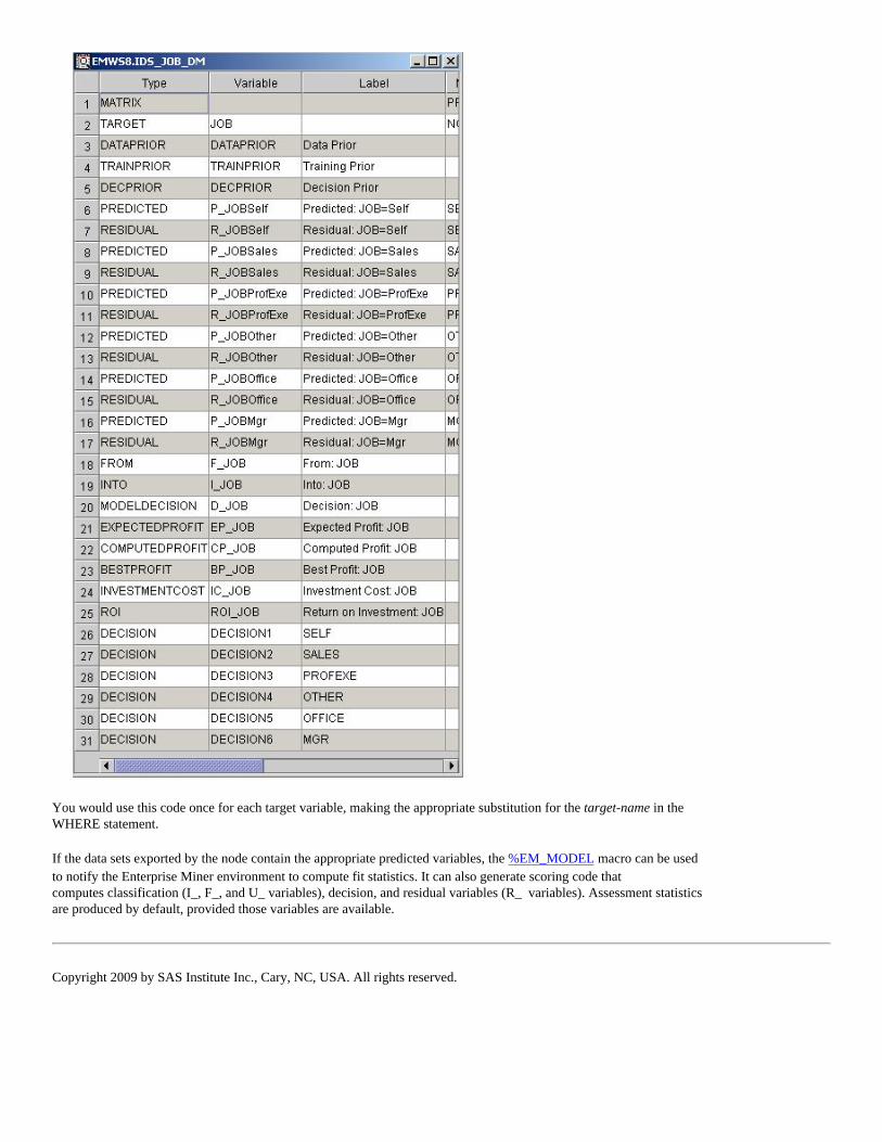
You would use this code once for each target variable, making the appropriate substitution for the target-name in the WHERE statement.

If the data sets exported by the node contain the appropriate predicted variables, the %EM_MODEL macro can be used to notify the Enterprise Miner environment to compute fit statistics. It can also generate scoring code that computes classification (I_, F_, and U_ variables), decision, and residual variables (R_ variables). Assessment statistics are produced by default, provided those variables are available.


Chapter 4: Extension Node Example This example builds an extension node that enables a user to access the functionality provided by the REG procedure of the SAS/STAT software. The node provides the user with the ability to control the selection technique used to fit the model. The user can also control how variables that are excluded from the final model are exported to successor nodes.

Icons

The following 32x32 and 16x16 pixel .gif files are used to generate the extension node icons:

When deployed, the icons appear on the toolbar and a process flow diagram as follows:

XML Properties File

The XML properties file for this example is as follows:


<Component type="AF" resource="com.sas.analytics.eminer.visuals.PropertyBundle" serverclass="EM6" name="Reg" displayName="Linear Regression" description="Fit linear regression model using the REG procedure." group="MODEL" icon="LinearRegressionPlane.gif" prefix="LReg" >

<PropertyDescriptors>

<Views> <View name="Train"> <PropertyRef nameref="Method"/> <PropertyRef nameref="Details"/> </View> <View name="Score"> <PropertyRef nameref="ExcludedVariables"/> </View></Views>

</Component>

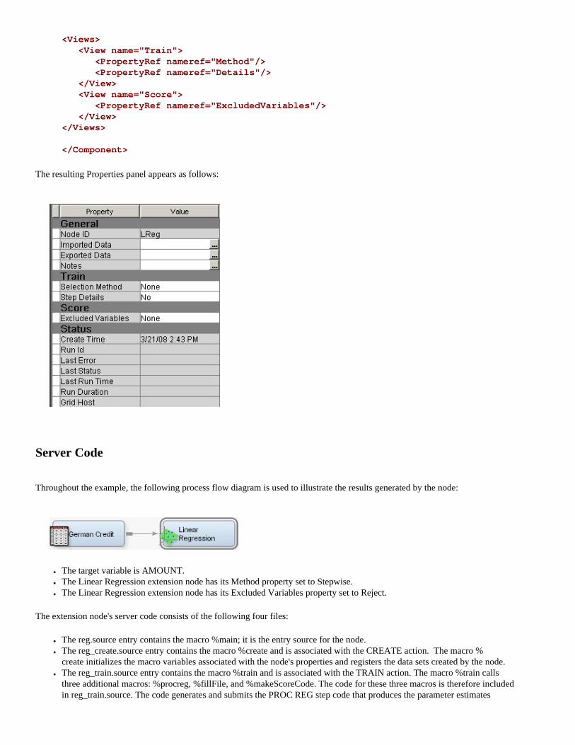
The resulting Properties panel appears as follows:

Server Code

Throughout the example, the following process flow diagram is used to illustrate the results generated by the node:

● The target variable is AMOUNT.● The Linear Regression extension node has its Method property set to Stepwise.● The Linear Regression extension node has its Excluded Variables property set to Reject.

The extension node's server code consists of the following four files:

● The reg.source entry contains the macro %main; it is the entry source for the node.● The reg_create.source entry contains the macro %create and is associated with the CREATE action. The macro %

create initializes the macro variables associated with the node's properties and registers the data sets created by the node. ● The reg_train.source entry contains the macro %train and is associated with the TRAIN action. The macro %train calls

three additional macros: %procreg, %fillFile, and %makeScoreCode. The code for these three macros is therefore included in reg_train.source. The code generates and submits the PROC REG step code that produces the parameter estimates

and generates the FLOW and PUBLISH scoring code. ● The reg_score.source entry contains the macro %score and is associated with the SCORE action. The macro %score

controls how variables that are excluded from the final model are exported from the node.

reg.source

%macro main;

%if %upcase(&EM_ACTION) = CREATE %then %do;

filename temp catalog 'sashelp.em61ext.reg_create.source'; %include temp; filename temp; %create;

%end;

%else %if %upcase(&EM_ACTION) = TRAIN %then %do;

filename temp catalog 'sashelp.em61ext.reg_train.source'; %include temp; filename temp; %train;

%end;

%if %upcase(&EM_ACTION) = SCORE %then %do;

filename temp catalog 'sashelp.em61ext.reg_score.source'; %include temp; filename temp; %score;

%end; %mend main;%main;

CREATE Action

When the CREATE action is called, the following code stored in the reg_create.source entry is submitted:

%macro create;

/* Training Properties */ %em_property(name=Method, value=NONE); %em_property(name=Details, value=N);

/* Scoring Properties */ %em_property(name=ExcludedVariable, value=REJECT, action=SCORE);

/* Register Data Sets */ %EM_REGISTER(key=OUTEST, type=DATA);

%EM_REGISTER(key=EFFECTS, type=DATA);

%mend create;

Using the &EM_PROPERTY macro, we define two Train properties and one Score property:

● Method is a String Property with a ChoiceList Control. The property indicates the model selection method that is used to obtain the final model. The initial value of the Method property is NONE, so by default, no selection method is used. The property has no action associated with it, so it is assumed to be a Train property.

● Details is a boolean Property. When set to Y, it indicates that statistics are to be listed in the output at the end of each step when a model selection method is used.

● ExcludedVariable is a String Property with a ChoiceList Control. The property indicates how the node exports variables that are not selected in the final model when using a model selection technique. By default, the value is REJECT, which means that such variables have their role set to REJECTED. This is a Score property because it does not affect the model or results produced by PROC REG. For performance reasons, we do not need to refit the linear regression model if the user changes the property to NONE or HIDE. By associating the property with a SCORE action, the node skips over the TRAIN action and simply rescores and regenerates the exported metadata.

The %EM_REGISTER macro is used to register the EFFECTS and the OUTEST data sets, which contain the parameter estimates from the linear regression model.

TRAIN Action

When the &EM_ACTION macro variable is set to TRAIN, the reg_train.source entry is executed. This extension node simply executes the REG procedure. The extension node has data requirements:

● There must be a training data set imported by the node. If not, an exception is thrown indicating that the user must specify a training data set. Note: In this example, the exception string has been set to an encoding string that is recognized by the SAS Enterprise Miner client.

● There must be an interval target variable. If not, an exception is thrown indicating that the user must specify an interval target variable.

The %EM_GETNAME macro is called to initialize the &EM_USER_OUTEST and &EM_USER_EFFECTS macro variables. These data sets are used to store the parameter estimates.

%macro train;

%if %sysfunc(index(&EM_DEBUG, SOURCE))>0 or %sysfunc(index(&EM_DEBUG, ALL))>0 %then %do; options mprint; %end;

%if (^%sysfunc(exist(&EM_IMPORT_DATA)) and ^%sysfunc(exist(&EM_IMPORT_DATA, VIEW))) or "&EM_IMPORT_DATA" eq "" %then %do; %let EMEXCEPTIONSTRING = exception.server.IMPORT.NOTRAIN,1; %goto doenda; %end;

%if (%EM_INTERVAL_TARGET eq ) %then %do; %let EMEXCEPTIONSTRING = exception.server.METADATA.USE1INTERVALTARGET; %goto doenda; %end;

%em_getname(key=OUTEST, TYPE=DATA);

%em_getname(key=EFFECTS, type=DATA);

%procreg;

%makeScoreCode;

%em_model(TARGET=&targetvar, ASSESS=Y, DECSCORECODE=Y, FITSTATISTICS=Y, CLASSIFICATION=N, RESIDUALS=Y);

%em_report(key=EFFECTS, viewtype=BAR, TIPTEXT=VARIABLE, X=VARIABLE, Freq=TVALUE, Autodisplay=Y, description=%nrbquote(Effects Plot), block=MODEL);

%doenda:

%mend train;

In the %procreg macro, we fit a linear regression model using the REG procedure:

● Using the ODS system, create the EFFECTS data set containing the parameter estimates.● If the Details property is set to Yes (corresponds to the &EM_PROPERTY_DETAILS macro variable), then the

DETAILS options of the MODEL statement is used.● The model uses all interval and rejected variables with the “Use” attribute set to “Yes”. Those variables are assigned

to the %EM_INTERVAL_INPUT and %EM_INTERVAL_REJECTED macros. ● If a frequency variable is defined, the FREQ statement is used.

%macro procreg;

%global targetVar; %let targetVar = %scan(%EM_INTERVAL_TARGET, 1, );

ods output parameterestimates= &EM_USER_EFFECTS;

proc reg data=&EM_IMPORT_DATA OUTEST=&EM_USER_OUTEST; model &targetVar = %EM_INTERVAL_INPUT %EM_INTERVAL_REJECTED

%if %upcase(&EM_PROPERTY_METHOD) ne NONE %then %do; selection= &EM_PROPERTY_METHOD

%end;

;

%if %EM_FREQ ne %then %do; freq %EM_FREQ; %end; run; ods _all_ close; ods listing;

%mend procreg;

The EFFECTS data set has the following structure:

Model Dependent Variable DF Estimate StdErr tValue Probt

MODEL1 amount Intercept 1 -1130.54625 534.48857 -2.12 0.0347 MODEL1 amount age 1 14.12780 5.53920 2.55 0.0109 MODEL1 amount duration 1 136.22034 5.32411 25.59 <.0001 MODEL1 amount employed 1 -108.10434 52.16738 -2.07 0.0385 MODEL1 amount foreign 1 567.01572 323.58225 1.75 0.0800 MODEL1 amount installp 1 -830.99671 54.44354 -15.26 <.0001 MODEL1 amount job 1 570.83009 103.14025 5.53 <.0001 MODEL1 amount property 1 263.71329 62.04117 4.25 <.0001 MODEL1 amount savings 1 56.29680 38.38939 1.47 0.1428 MODEL1 amount telephon 1 642.84575 135.33767 4.75 <.0001

You can easily generate the scoring code using this data set.

The OUTEST data set contains the parameter estimates for variables in the final model, but also identifies variables that are excluded from the model. It has the following structure:

_MODEL_ _TYPE_ _DEPVAR_ _RMSE_ Intercept age checking coapp depends

MODEL1 PARMS amount 1892.16 -1130.55 14.1278 . . .

The %makeScoreCode macro retrieves the name of the predicted variable using the decision metadata data set. If only one target variable is defined, that data set corresponds to the &EM_DEC_DECMETA macro variable. If multiple target variables are defined, you can retrieve the decision metadata data set from the &EM_TARGETDECINFO data set.

The %fillfile macro processes the EFFECTS data set, generates the scoring code, and saves it in the &EM_FILE_EMPUBLISHSCORECODE and &EM_FILE_FLOWSCORECODE files that correspond to the Publish and Flow scoring code, respectively.

%macro fillFile(type=, predVar=, file=); filename tempf "&file"; data _null_; file tempf; set &EM_USER_EFFECTS end=eof; if _N_=1 then do; put "&predVar = "; if Variable = 'Intercept' then put Estimate; else put Estimate '*' Variable; end; else do; put '+' Estimate '*' Variable; end; if eof then do; put ";"; end; run; filename tempf;%mend fillFile;

%macro makeScoreCode; %let predvar=;

%if &em_dec_decmeta eq %then %do; %if %sysfunc(exist(EM_TARGETDECINFO)) %then %do; data _null_; set EM_TARGETDECINFO; where TARGET="&targetVar"; call symput('em_dec_decmeta', DECMETA); run; %end; %end; %if (&em_dec_decmeta ne ) and %sysfunc(exist(&em_dec_decmeta)) %then %do; data _null_; set &em_dec_decmeta; where _TYPE_ = 'PREDICTED'; call symput('predVar', strip(VARIABLE)); call symput('predLabel', strip(LABEL)); run; %end;

%if &predVar eq %then %goto doendm;

%fillFile(type=publish, predvar=&predVar, file=&EM_FILE_EMPUBLISHSCORECODE); %fillFile(type=flow, predvar=&predVar, file=&EM_FILE_EMFLOWSCORECODE);

%doendm:%mend makeScoreCode;

The generated scoring code has the following form:

P_amount = -1130.54625+14.12780 *age+136.22034 *duration+-108.10434 *employed+567.01572 *foreign+-830.99671 *installp+570.83009 *job+263.71329 *property+56.29680 *savings+642.84575 *telephon;

The %em_model macro is used to generate additional scoring code and to produce assessment reports.

%em_model(TARGET=&targetvar, ASSESS=Y, DECSCORECODE=Y, FITSTATISTICS=Y, CLASSIFICATION=N, RESIDUALS=Y);

● ASSESS=Y — indicates to generate assessment reports (Score Rankings and Score Distribution).● DECSCORECODE=Y — indicates to append score code to generate decision variables when a profit matrix is defined.● FITSTATISTICS=Y — indicates to compute fit statistics associated with the model. Those are computed for the training

data set and for validation and test data sets when applicable.● CLASSIFICATION=N — indicates not to generate report and score code associated with the classification variables (I_).● RESIDUALS=Y — indicates to append the code generating the residual variable (R_) to the flow score code and produce

the residual report.

For example, the Flow scoring code would now appear as follows:

P_amount = -1130.54625+14.12780 *age+136.22034 *duration+-108.10434 *employed+567.01572 *foreign+-830.99671 *installp+570.83009 *job+263.71329 *property+56.29680 *savings+642.84575 *telephon;*------------------------------------------------------------*;*Computing Residual Vars: amount;*------------------------------------------------------------*;Label R_amount = 'Residual: amount';R_amount = amount - P_amount;

The %em_report macro generates a graph of the parameter estimates:

%em_report(key=EFFECTS, viewtype=BAR, TIPTEXT=VARIABLE, X=VARIABLE, Freq=TVALUE, Autodisplay=Y, description=%nrbquote(Effects Plot), block=MODEL);

● Key=EFFECTS — identifies the data set used to produce the chart.● Viewtype=BAR — indicates to generate a BAR graph.● TIPTEXT=VARIABLE — indicates that the variable named VARIABLE is to be used to identify a bar when clicking on it.● X=VARIABLE — indicates that the bar chart should have one bar for each variable.● FREQ=TVALUE — specifies that the variable TVALUE should be used to control the height of the various bar.● AutoDisplay=Y — indicates to display the report whenever the Results viewer of the node is opened.● Description==%nrbquote(Effects Plot) — specifies the title bar of the report.● Block=MODEL — indicates that the report should appear under the “Model” pmenu item.

Score Action

When the &EM_ACTION macro variable is set to SCORE, the reg_score.source entry is executed.

The %em_getname macro is used again to retrieve the &em_user_outest macro variable. This is done because the training code might not be running before executing the SCORE action. For example, if the ExcludedVariable is the only modified property, the TRAIN action would be bypassed.

If the user specifies a model selection method using the Method property and sets the ExcludedVariable property to either HIDE or REJECT, the node generates DATA step code that modifies the metadata that is exported to successor nodes. The DATA step code is saved in the &EM_FILE_CMETA_TRAIN file.

Using PROC TRANSPOSE of Base SAS, the node identifies all the variables with missing parameter estimates. Those are variables excluded from the final model. If the ExcludedVariable property is set to REJECT, then the role of the variables with missing parameter estimates is set to REJECTED. If the ExcludedVariable property is set to HIDE, variables with missing parameter estimates are deleted from the exported metadata so that successor nodes are not exposed to those variables.

%macro score;

/* Delete Code Modifying Exported Metadata */ filename tempd "&EM_FILE_CDELTA_TRAIN"; data _null_; if fexist('tempd') then rc=fdelete('tempd'); run;

%if (%upcase("&EM_PROPERTY_METHOD") ne "NONE") and (%upcase("&EM_PROPERTY_EXCLUDEDVARIABLE") ne "NONE") %then %do;

%em_getname(key=OUTEST, type=DATA); proc transpose data=&EM_USER_OUTEST out=temp(where=(Col1 eq .)); run; data _null_; file tempd; length String $200; set temp end=eof; if _N_=1 then put 'if upcase(NAME) in('; string = quote(strip(upcase(_NAME_))); put string; if eof then do;

%if %upcase("&EM_PROPERTY_EXCLUDEDVARIABLE") eq "REJECT" %then %do; put ') then ROLE="REJECTED";'; %end; %else %do; put ') then delete;'; %end; end; run;

%end;

filename tempd;

%mend score;

For example, the generated “delta code” could have the following form:

if upcase(NAME) in("CHECKING""COAPP""DEPENDS""EXISTCR""HISTORY""HOUSING""MARITAL""OTHER""RESIDENT") then ROLE="REJECTED";


Chapter 5: Deploying An Extension Node This chapter provides a concise reference for all extension node deployment issues.

There are two paths for extension nodes deployment, depending on the SAS Enterprise Miner installation you choose:

● Personal Workstation● Shared Platform Server

The required components for extension nodes are as follows:

● a SAS catalog containing the extension node's entry source file ● two images per node:

�❍ a 16x16 pixel image used on the Enterprise Miner SEMMA toolbar�❍ a 32x32 pixel image used to represent the node in the Enterprise Miner

diagram workspace● an XML properties file

Personal Workstation System

Use the following steps to deploy extension nodes on a SAS Enterprise Miner Personal Workstation installation:

1. Close the Enterprise Miner Client application. 2. Copy the XML properties file to the ext directory that is under the SAS

configuration directory:

...\SAS\Config\Levn\analyticsPlatform\apps\EnterpriseMiner\ext

3. Copy the 16x16 and 32x32 pixel images to the gif16 and gif32 directory, respectively:

...\SAS\Config\Levn\analyticsPlatform\apps\EnterpriseMiner\ext\gif16


4. Place the SAS catalog containing your node's source code entry file in a SAS library that is accessible by the SAS Enterprise Miner server.

5. Restart the Enterprise Miner Client application.

If you make changes to the icon images or the XML properties file, you must close and reopen the client in order for the changes to take effect. You should also close any open diagram before you close the client.

Shared Platform Server

Follow these steps to deploy extension nodes on the Enterprise Miner Shared Analytics Platform Server. You do not need to update each individual end-user client.

1. Notify the users to close their Enterprise Miner Client sessions before you stop the Analytics Platform. Verify that all the client sessions have been shut down.

2. Log on as a System Administrator or as a member of the Administrators group.

3. Stop the Enterprise Miner Analytics Platform. Select Start Programs SAS SAS Configuration Config-Lev1 Analytics Platform-Stop

4. Copy the node's XML properties file to the ext directory that is under the SAS configuration directory.

...\SAS\Config\Levn\analyticsPlatform\apps

\EnterpriseMiner\ext

5. Copy the 16x16 and 32x32 pixel images to the following directories, respectively:



6. Place the SAS catalog containing your node's source code entry file in a SAS library that is accessible by the SAS Enterprise Miner server.

7. Restart the Enterprise Miner Shared Analytics Platform. Select Start Programs SAS SAS Configuration Config-Lev1 Analytics Platform-Start

If you make changes to the icon images or the XML properties file, you must stop and restart the AP server in order for the changes to take effect.

Making Your Server Code Accessible to SAS Enterprise Miner

If you follow the development strategy described in previous chapters, the source code for your extension node consists of multiple files. As a practical matter, it is most convenient for the purposes of development and deployment if all of the files reside in a single SAS catalog. Deploying the code is then just a matter of placing the catalog in a SAS library that is accessible by SAS Enterprise Miner.

The simplest method is to include your catalog in the SASHELP library. This is accomplished in one of three ways. The first way is to use PROC CATALOG. Suppose your catalog is named mylib.mycode. Start a SAS session and issue the commands:

proc catalog cat=mylib.mycode; copy out=sashelp.mycode;

run;

The second way is to manually copy and paste the catalog into the SASCFG folder. The exact location of this folder depends upon your operating system and your installation configuration, but it is always found under the root SAS directory and has a path resembling the following:

C:\Program Files\SAS\SASFoundation\9.2\nls\en\SASCFG

The third way is to store the catalog in another folder and then modify the SAS system configuration file SASV9.CFG. The folder containing the catalog is then included in the SASHELP search path. The SASV9.CFG file is located under the root SAS directory:

C:\Program Files\SAS\SASFoundation\9.2\nls\en

The advantage of putting your code in the SASHELP library is that anyone using that server has access to it.

An alternative is to place your code in a separate folder and issue a LIBNAME statement. The library needs to be accessible when a project is opened. See Appendix 4: Allocating Libraries for SAS Enterprise Miner 6.1 for details on the various ways this can be accomplished. For a shared platform installation, the catalog must reside on the SAS Enterprise Miner server. For a personal workstation installation, the catalog resides on the client, because the client and server are the same machine.

If you have more than one extension node, you can place the code for all of your extension nodes in a single catalog. However, while you are developing an extension node, it is probably better to keep that node's code in a separate catalog. That way, as you are developing or modifying the node's code, you do not have to interrupt the use of other extension nodes.

Batch Mode

SAS Enterprise Miner enables you to execute a process flow in batch mode using the %EM5BATCH macro. As indicated previously, when running in batch mode, Enterprise Miner does not process a node's XML properties file. As such, Enterprise Miner has no way of determining where the source code for an extension node resides. Therefore, if

you plan to use an extension node in a batch process, you must provide Enterprise Miner with a means to locate the source code for your extension node. This is accomplished by creating a SAS data set named Extension. The data set must contain two character variables named Component and Code. There is one observation for each extension node that you create. The Component variable contains the name of the extension node. This should be the same as the value of the name attribute in the Component element of the node's XML properties file. The Code variable contains the name of the source file that serves as the entry point for your extension node. It is the same as the value of the initial attribute of the Catalog Property element of the node's XML properties file. The Extension data set must be stored in a SAS library name Emgmeta. When you use an extension node in a batch process, SAS Enterprise Miner automatically checks for the existence of the Emgmeta library and the Extension data set. When it exists, the Extension data set is read to determine the location of the extension node's entry point source code. For example, if your node is named Reg and the entry point source code is a file named Sashelp.Em61ext.reg.source, the data set Extension has the value of Reg for the Component variable and the value Sashelp.Em61ext.reg.source for the Code variable.


SAS Code Node

● Overview of the SAS Code Node ● SAS Code Node Properties ● Code Editor

�❍ User Interface�❍ Macros�❍ Macro Variables�❍ Code pane

● SAS Code Node Results ● SAS Code Node Examples

Overview of the SAS Code Node

The SAS Code node enables you to incorporate new or existing SAS code into process flow diagrams that were developed using Enterprise Miner. The SAS Code node extends the functionality of Enterprise Miner by making other SAS System procedures available for use in your data mining analysis. You can also write SAS DATA steps to create customized scoring code, conditionally process data, or manipulate existing data sets. The SAS Code node is also useful for building predictive models, formatting SAS output, defining table and plot views in the user interface, and for modifying variables metadata. The SAS Code node can be placed at any location within an Enterprise Miner a process flow diagram. By default, the SAS Code node does not require data. The exported data that is produced by a successful SAS Code node run can be used by subsequent nodes in a process flow diagram.

SAS Code Node Properties

When the SAS Code node is selected in the Diagram Workspace, the Properties panel displays all of the properties that the node uses and their associated values.

● SAS Code Node General Properties ● SAS Code Node Train Properties ● SAS Code Node Score Properties ● SAS Code Node Status Properties

SAS Code Node General Properties

The following general properties are common to all SAS Enterprise Miner nodes.

● Node ID — displays the ID of the node. ● Imported Data — Select the button to open a table of SAS data sets that are imported into the SAS Code node. If

data exists for an imported data source, you can select the row in the imported data table and click one of the following buttons: �❍ Browse — opens a window where you can browse the data set. �❍ Explore — opens a window where you can sample and plot the data. �❍ Properties — opens the Properties panel for the data source. The Properties panel contains a Table tab and a Variables

tab. The tabs contain summary information (metadata) about the table and the variables. ● Exported Data — Select the button to open a table of SAS data sets that are exported data by the SAS Code node. If

data exists for an exported data set, you can select the row in the table and click one of the following buttons: �❍ Browse — opens a window where you can browse the data set. �❍ Explore — opens the Explore window, where you can sample and plot the data. �❍ Properties — opens the Properties panel for the data set. The Properties panel contains a Table tab and a Variables tab.

The tabs contain summary information (metadata) about the table and the variables. ● Notes — Select the button to the right of the Notes property to open a window that you can use to store notes of

interest, such as data or configuration information.

SAS Code Node Train Properties

The following train properties are associated with the SAS Code node.

● Variables — Use the Variables table to specify the status for individual variables that are imported into the SAS Code node. Select the button to open a window containing the variables table. You can set the Use and Report status for individual variables, view the columns metadata, or open an Explore window to view a variable's sampling information, observation values, or a plot of variable distributions. You can apply a filter based on the variable metadata column values so that only a subset of the variables is displayed in the table.

● Code Editor — Select the button to open the Code Editor. You can use the Code Editor to edit and submit code interactively while viewing the SAS log and output listings. You can also run a process flow diagram path up to and including the SAS Code node and view the Results window without closing the programming interface. For more details, see the Code Editor section below.

● Tool Type — specifies the node type using the Enterprise Miner SEMMA framework. Valid values are: �❍ Sample �❍ Explore�❍ Modify�❍ Model�❍ Assess�❍ Utility.

The default setting for the Tool Type property is Utility. When the Tool Type is set to Model, Enterprise Miner creates a target profile for the node is none exists. It will also create a report data model that is appropriate for a modeling node. Doing so allows SAS Enterprise Miner to automatically generate assessment results provided certain variables are found in the scored data set (P_, I_, F_, R_ (depending on the target level)). See Predictive Modeling for more details regarding these variables and other essential information regarding modeling nodes.

● Data Needed — specifies whether the node needs at least one predecessor node. Valid values are Yes and No. The default setting for the Data Needed property is No.

● Rerun — specifies whether the node should rerun each time the process flow is executed, regardless of whether the node has run before or not. Valid values are Yes and No. The default setting for the Rerun property of the SAS Code node is No.

● Use Priors — specifies whether the posterior probability values are adjusted by the prior probability values. Valid values for the Use Priors property are Yes and No. The default setting for the Use Priors property is Yes.

SAS Code Node Score Properties

The following score properties are associated with the SAS Code node.

● Advisor Type — specifies the type of Enterprise Miner input data advisor to be used to set the initial input variable measurement levels and roles. Valid values are

�❍ Basic — any new variables created by the node will inherit Basic metadata attributes. These attributes include:

■ character variables are assigned a Level of Nominal■ numeric variables are assigned a Level of Interval■ variables are assigned a Role of Input

�❍ Advanced — variable distributions and variable attributes are used to determine the variable level and role attributes of

newly created variables. The default setting for the Advisor Type property is Basic. You can also control the metadata programmatically by writing SAS code to the file CDELTA_TRAIN.sas. There is also a feature that permits a user to create a dataset that predefines metadata for specific variable names. This dataset must be named COLUMNMETA and it must be stored in the EMMETA library.

● Publish Code — specifies the file that should be used when collecting the scoring code to be exported. Valid values are

�❍ Flow — Flow scoring code is used to score SAS data tables inside the process flow diagram. The scoring code is written to EMFLOWSCORE.sas.

�❍ Publish — Publish scoring code is used to publish the Enterprise Miner model to a scoring system outside the process flow diagram. The scoring code is written to EMPUBLISHSCORE.sas.

The default setting of the Publish Code property is Publish. It is possible to have scoring code that is used within the process flow (Flow code) and different code that is used used to score external data (Publish code). For example, when generating Flow code for modeling nodes, the scoring code can reference the observed target variable and you can generate residuals from a statistical model. Since Publish code is destined to be used to score external data where the target variable is unobserved, residuals from a statistical model cannot be generated.

● Code Format — specifies the format of the score code to be generated. Valid values are:

�❍ DATA step — The score code contains only DATA step statements.�❍ Other — The score code contains statements other than DATA step statements, such as PROC step statements.

The default setting for the Code Format property is DATA step. It is necessary to make the distinction because nodes such as the Ensemble node and the Score node collect score code from every predecessor node in the process flow diagram. If all of the predecessor nodes generate only DATA step score code, then the score code from all of the nodes in the process flow diagram can simply be appended together. However, if PROC step statements are intermixed in the score code in any of the predecessor nodes, a different algorithm must be employed.

SAS Code Node Status Properties

The following status properties are common to all SAS Enterprise Miner nodes.

● Create Time — displays the time that the SAS Code node was created. ● Run ID — displays the training identifier. A new identifier is created every time the node is run. ● Last Error — displays the error message from the last run. ● Last Status — displays the last reported status of the node. ● Last Run Time — displays the time at which the node was last run. ● Run Duration — displays the length of time of the last node run. ● Grid Host — displays the grid host used for computation. ● User-Added Node — specifies if the node was created by a user as a SAS Enterprise Miner extension node.

Code Editor

You use the Code Editor to enter SAS code that executes when you run the node. The editor provides separate panes for Train, Score, and Report code. You can edit and submit code interactively in all three panes while viewing the SAS log and output listings. You can also run the process flow diagram path up to and including the SAS Code node and view the Results window without closing the programming interface.

The Code Editor provides tables of macros and macro variables that you can use to integrate your SAS code with the Enterprise Miner environment. You use the macro variables and the variables macros to reference information about the imported data sets, the target and input variables, the exported data sets, the files that store the scoring code, the decision metadata, and so on. You use the utility macros, which typically accept arguments, to manage data and format output. You can insert a macro variable, a variables macro, or a utility macro into your code without having to type its name; you simply select an item from the macro variables list or macros table and drag it to the active code pane.

If an imported data set exists, you can access the variables table from the Code Editor. The variables table has the same functionality regardless of whether it is accessed from the Code Editor or the SAS Code node's Properties panel.

You can also access the SAS Code node's Properties panel from the Code Editor. You can specify values for any of the node's properties in the Code Editor's properties interface the same way you would in the SAS Code node's Properties panel.

User Interface

The Code Editor consists of seven components. Some components serve multiple functions:

1. Menu2. Toolbar3. Content Selector Buttons4. Tables Pane

�❍ Macros table�❍ Macro variables table�❍ Variables table

5. Code Pane �❍ Training Code�❍ Score Code�❍ Report Code

6. Results Pane �❍ Output�❍ Log

7. Status Bar

Menu

The Code Editor menu consists of the following items:

● File �❍ Save — save the contents in the current view of the code pane.�❍ Save As — saves any combination of the code, output or log.�❍ Save All — saves the code, output, and log.�❍ Print — print the contents of the pane that currently has the focus.�❍ Exit — close the Code Editor window and return to the Enterprise Miner main workspace.

● Edit �❍ Cut — deletes the selected item and copies it to the clipboard.�❍ Copy — copies the selected item to the clipboard.�❍ Paste — pastes a copied item from the clipboard.�❍ Select All — selects all of the text from the code pane.

�❍ Clear All — clears all of the text from the current code pane.�❍ Find and Replace — opens the Find/Replace dialog box allowing you to search for and replace text in the

code, output, and log.● Run

�❍ Run Code — runs the code in the active code pane. This does not affect the status of the node or the process flow. It is simply a way to validate your code.

�❍ Run Node — runs the SAS Code node and any predecessor nodes in the process flow that have not been executed.

�❍ Results — open the SAS Code node's Results window.�❍ Stop Node — interrupts a currently running process flow.

● View �❍ Training Code — views the Training Code pane.�❍ Score Code — views the Score Code pane.�❍ Report Code — views the Report Code pane.�❍ Properties — open the SAS Code node Properties panel.

Toolbar

● — saves the contents in the current view of the code pane

● — saves the contents of the code pane, the output, and the SAS log

● — prints the contents of the code pane, the output, or the SAS log

● — runs the code in the active code pane

● — runs the SAS Code node and any predecessor nodes in the process flow that have not been executed

● — opens the SAS Code node's Results window

● — stops a currently running process flow diagram

● — resets the workspace

Content Selector Buttons

● — displays the SAS Code node Training Code

● — displays the SAS Code node Score Code

● — displays the SAS Code node Report Code

● — opens the property settings for the SAS Code node

Tables Pane

● Macros — Click the Macros tab to view a table of macros in the Tables pane. The macro variables are arranged in two groups: Utility and Variables. Click on the plus or minus sign on the left of the group name to expand or collapse the list, respectively. You can insert a macro into your code without typing its name by selecting an item from the macros table, and dragging it to the code pane.

● Macro Variables — Click the Macro Variables tab to view a table of macro variables in the Tables pane. You can use the split bar to adjust the width of the columns in the table. For many of the macro variables, you will see the value to which it resolves in the Value column, but in some cases, the value cannot be displayed in the table since those macro variables are populated at run-time.

The macro variables are arranged in groups according to function:

�❍ General — Use general macro variables to retrieve system information. �❍ Properties — Use properties macro variables to retrieve information about the nodes. �❍ Imports — Use imports macro variables to identify the SAS tables that are imported from predecessor

nodes at run time. �❍ Exports — Use exports macro variables to identify the SAS tables that are exported to successor nodes at

run time.�❍ Files — Use files macro variables to identify external files that are managed by Enterprise Miner, such as

log and output listings.�❍ Number of Variables — Use number of variables macro variables for a given combination of the

measurement levels and model roles. �❍ Statements — Use statements macro variables to identify SAS program statements that are frequently

used by Enterprise Miner, such as the decision statement in the modeling procedures.�❍ Code Statements — Use the Code Statements macro variable to identify the file containing the Code

statement.

You can insert a macro variable into your code without typing its name by selecting an item from the macro variables table, and dragging it to the code pane.

● Variables — Click on the Variables tab to view the variables table in the Tables pane. The variables table has the

same functionality regardless of whether it is accessed from the Code Editor or the SAS Code node's Properties panel.

Code Pane

The Code pane has three views: Training Code, Score Code, and Report Code.

Click on the (Training), (Score), or (Report) icons on the toolbar to choose the pane in which you want to work.

The code from the three panes is executed sequentially when you select Run Node ( ). Training code is

executed first, followed by Score code, and then Report code. If you select Run Code ( ), only the code in the visible code pane is executed. For more details, see the Code pane section.

Use the controls to either expand ( ) or collapse ( ) the code pane.

Results Pane

The Results pane has two tabs: Output and Log. Click the Output tab to view the output generated by your code or click

the Log tab to view the SAS Log that was generated by your code. If you run the node ( ), rather than just your code (

), the output and log must be viewed from the SAS Code node's Results window ( ) and not from the Code Editor's Results pane.

Use the controls to either expand ( ) or collapse ( ) the Results pane.

Status Bar

The status bar displays the following:

● SAS User ID — the SAS User ID of the current Enterprise Miner session owner.● User name — the User name that is associated with the current Enterprise Miner session owner.● Project name — the name of the currently open Enterprise Miner project.● Diagram name — the name of the currently open Enterprise Miner diagram.● Node name — the name of the selected node in the current Enterprise Miner diagram workspace.● Current status — the current status of the selected node in the current Enterprise Miner diagram

workspace.● Last status — the last known status of the selected node in the current Enterprise Miner diagram

workspace.

Macros

The Macros table lists the SAS macros that are used to encode multiple values, such as a list of variables, and functions that are already programmed in Enterprise Miner. The macro variables are arranged in two groups: Utility and Variables. Utility macros are used to manage data and format output and Variables macros are used to identify variable definitions at run time. The macros discussion below is organized as follows:

● Utility Macros

�❍ %EM_REGISTER�❍ %EM_REPORT�❍ %EM_MODEL�❍ %EM_DATA2CODE�❍ %EM_DECDATA�❍ %EM_CHECKMACRO�❍ %EM_CHECKSETINIT�❍ %EM_ODSLISTON�❍ %EM_ODSLISTOFF �❍ %EM_METACHANGE�❍ %EM_GETNAME�❍ %EM_CHECKERROR�❍ %EM_PROPERTY

● Variables Macros

Utility Macros

Use utility macros to manage data and format output. The following utility macros are available:

%EM_REGISTER

Use the %EM_REGISTER macro to register a unique file key. When you register a key, Enterprise Miner generates a macro variable named &EM_USER_key. You then use &EM_USER_key in your code to associate a file with the key. Registering a file allows Enterprise Miner to track the state of the file, avoid name conflicts, and insure that the registered file is deleted when the node is deleted from a process flow diagram.

%EM_REGISTER allows the following arguments:

ACTION = < TRAIN | SCORE | REPORT > — associates the registered CATALOG, DATA, FILE, or FOLDER with an action. If the registered object is modified, the associated action is triggered to execute whenever the node is run subsequently. The default value is TRAIN. This is an optional argument. The argument has little use in the SAS Code node but can be of significant value to extension node developers.

AUTODELETE = <Y|N> — Request the delete status of the file prior to the run. This argument is optional.

EXTENSION = <file-extension> — an optional parameter to identify non-standard file extensions (.sas or .txt, for example).

FOLDER = <folder-key> — the folder key where a registered file resides (optional).

KEY = <data-key> — an alias for a filename.

PROPERTY = <Y|N> — an optional argument that indicates that the file is a node property and that when the node or the process flow diagram is exported, the content of the registered file will also be exported with the rest of the properties.

TYPE = <CATALOG | DATA | FILE | FOLDER> — the type of file that is to be registered.

For example, if you want to use the data set Class from the SASHELP library, register the key Class:

%em_register(key=Class, type=data);

Later, in your code, you can use statements like

data &em_user_Class;set Sashelp.Class;

so that references to &EM_USER_Class would resolve to the permanent data set Sashelp.Class.

%EM_REPORT

Use the %EM_REPORT macro to specify the contents of a results window display created using a registered data set. The display contents, or view, can be a data table view or a plot view. Examples of plot types are histogram, bar chart, and line plots. The views (both tables and plots) appear in the results window of the SAS Code node and in any results package files (SPK files).

%EM_REPORT allows the following arguments:

AUTODISPLAY = <Y | N> — specifies whether the report displays automatically when the results viewer is opened.

BLOCK = <group-name> — specifies the group that the report belongs to when the results viewer is opened. The default setting is CUSTOM.

COLOR = <variable-name> — specifies a variable that contains color value.

COMPARE = <Y | N> — specifies whether data in the generated report can be used to compare registered models. The default setting is N.

DESCRIPTION = <window-title-description> — specifies a text string or report description that will appear in the window title.

DISCRETEX = <Y | N> — specifies whether the values on the x-axis will be discrete when the VIEWTYPE is HISTOGRAM.

DISCRETEY = <Y | N> — specifies whether the values on the y-axis will be discrete when the VIEWTYPE is HISTOGRAM.

EQUALIZECOLX = <Y | N> — specifies if the x-axis should be equalized (that is, use a shared common scale and tick marks) across columns of the lattice. The default setting is N.

EQUALIZECOLY = <Y | N> — specifies if the y-axis should be equalized across columns of the lattice. The default setting is N.

EQUALIZEROWX = <Y | N> — specifies if the x-axis should be equalized (that is, use a shared common scale and tick marks) across rows of the lattice. The default setting is N.

EQUALIZEROWY = <Y | N> — specifies if the y-axis should be equalized across rows of the lattice. The default setting is N.

FREQ = <frequency-variable-name> — specifies a frequency variable.

GROUP = <group-variable-name(s)> — specifies one or more grouping variables.

IDVALUE = <data-set-name> — specifies a data set. When a corresponding variable name is specified using the REPORTID argument, a report is generated for each value of the specified variable in the named data set. A report window is created for each unique value.

KEY == <data-key> (required) — specifies the data key. Since this is a required argument, you must assign the data key using %EM_REGISTER before using %EM_REPORT.

LATTICETYPE=<viewtype> — valid viewtypes are:

● Data● Scatter● Lineplot● Bar● Histogram● Pie● Profileview● Gainsplot

LATTICEX =<lattice-row-variable-name> — specifies variables to be used as rows in a lattice.

LATTICEY = <lattice-column-variable-name> — specifies variables to be used as columns in a lattice.

LOCALIZE = <Y | N> — specifies whether the description should be localized or used as-is. The default setting is N.

REPORTID = <variable-name> — specifies a variable name. When a corresponding data set name is specified using the IDVALUE argument, a report is generated for each value of the specified variable in the named data set. A report window is created for each unique value.

SPK = <Y | N> — specifies whether to include the report and data in an SPK package. The default setting is Y.

SUBGROUP = <subgroup-variable-name(s)> — specifies one or more sub-grouping variables.

TIPTEXT = <variable-name> — specifies a variable that contains tooltip text.

TOOLTIP = <variable-name> — specifies a variable containing tooltip text for the Constellation application.

VIEWS = <numeric-value> — assigns a numeric ID to the generated report.

VIEWTYPE = < plot-type > — specifies the type of plot that you want to display. Valid plot types include:

● Data● Bar

● Histogram ● Lineplot● Pie● Profileview● Scatter● Gainsplot ● Lattice● Dendrogram● Constellation

Data is the default value.

WHERE = — specifies an explicit SQL WHERE clause.

X = <x-variable-name> — specifies the x-axis variable.

XREF = <numeric-value> — specifies a reference line on the x-axis.

Y = <y-variable-name> — specifies the y-axis variable.

Yn = <Yn-variable-name> — where n is an integer ranging from 1 to 16. Y1, Y2, ... , Y16 specify variables that are to be plotted and overlayed on the y-axis.

YREF = <numeric-name> — specifies a reference line on the y-axis.

Z = <z-variable-name> — specifies the z-axis variable of a 3-dimensional plot.

Examples using %EM_REPORT are provided below.

%EM_MODEL

The %EM_MODEL macro enables you to control the computations that are performed and the score code that is generated by the Enterprise Miner environment for modeling nodes. The macro supports the following arguments:

TARGET = <target-variable-name> — name of the target (required).

ASSESS = <Y|N> — assess the target. The default is Y.

DECSCORECODE = <Y|N> — generate decision score code. The default is N.

FITSTATISTICS = <Y|N> — compute fit statistics. The default is N.

CLASSIFICATION = <Y|N> — generate score code to generate classification variables (I_, F_, U_) . The default is N.

RESIDUALS = <Y|N> — generate score code to compute residuals. The default is N.

PREDICTED = <Y|N> — indicates if the node generates predicted values. The default is Y.

For example, suppose you have a binary target variable named BAD and your code only generates posterior variables. You can use the %EM_MODEL macro to indicate that you want Enterprise Miner to generate fit statistics, assessment statistics, and to generate score code that computes classification, residual, and decision variables.

%em_model( target=BAD, assess=Y, decscorecode=Y, fitstatistics=Y, classification=Y,

residuals=Y, predicted=Y);

NOTE: %EM_MODEL is available for use in your code but it does not currently appear in the Code Editor's table of macros.

%EM_DATA2CODE

The %EM_DATA2CODE macro converts a SAS data set to SAS program statements. For example, it can be used to embed the parameter estimates that PROC REG creates directly into scoring code. The resulting scoring code can be deployed without need for an EST data set. You must provide the code to use the parameter estimates to produce a model score.

%EM_DATA2CODE accepts the following arguments:

APPEND= <Y | N> — specifies whether to append or overwrite code if the specified file already exists.

DATA= <source-data-name> — specifies the source data.

OUTDATA= <output-data-set-name> — specifies the name of the output data set that is created when the DATA step code runs.

OUTFILE= <output-data-step-code-filename> — specifies the name of the output file that will contain the generated SAS DATA step code.

%EM_DECDATA

The %EM_DECDATA macro uses information that you entered to create the decision data set that is used by Enterprise Miner modeling procedures. %EM_DECDATA copies the information to the WORK library and assigns the proper type (profit, loss, or revenue) for modeling procedures.

%EM_DECDATA accepts the following arguments:

DECDATA = <decision-data-set> — specifies the data set containing the decision data set.

DECMETA = <decision-metadata — specifies the data set containing decision metadata.

NODEID = <node-identifier> — specifies the unique node identifier.

%EM_CHECKMACRO

Use the EM_CHECKMACRO macro to check for the existence of a macro variable. Assigning a value is optional.

%EM_CHECKMACRO accepts the following arguments:

NAME = <macro-variable-name> — specifies the name of the macro variable for which you want to check .

GLOBAL = <Y | N> — specifies whether the named macro variable is a global macro variable.

VALUE = <variable-value> — specifies a value for the macro variable if it has not been previously defined.

%EM_CHECKSETINIT

Use the %EM_CHECKSETINIT macro to validate and view your SAS product licensing information.

%EM_CHECKSETINIT has the following required argument:

PRODUCTID = <product id number> — specifies the product identification number. If the product specified is not licensed, SAS Enterprise Miner will issue an error and halt execution of the program.

%EM_ODSLISTON

Use the %EM_ODSLISTON macro to turn the SAS Output Delivery System (ODS) listing on, and to specify a name for the destination HTML file.

%EM_ODSLISTON accepts the following arguments:

FILE = <destination-file> — specifies the name of an HTML output file that will contain the generated ODS listing.

%EM_ODSLISTOFF

Use the %EM_ODSLISTOFF utility macro to turn SAS ODS listing off. No argument is needed for this macro.

%EM_METACHANGE

Use the %EM_METACHANGE macro to modify the columns metadata data set that is exported by a node. The macro should be called during either the TRAIN or SCORE actions. %EM_METACHANGE allows the following arguments:

NAME = <variable-name> — the name of the variable that you want to modify (required).

ROLE = <variable-role> — assign a new role to the variable (optional).

LEVEL = <UNARY | BINARY | ORDINAL | NOMINAL | INTERVAL> — assign a new measurement level to the variable (optional).

ORDER = <ASC | DESC | FMTASC | FMTDESC> — new level ordering for a class variable (optional).

COMMENT = <string>— string that can be attached to a variable (optional).

LOWERLIMIT = <number> — the lower limit of a numeric variable's valid range (optional).

UPPERLIMIT = <number> — the upper limit of a numeric variable's valid range.

DELETE = <Y|N> — indicate whether the variable should be removed from the metadata (optional).

%EM_GETNAME

Use %EM_GETNAME to retrieve the name of a file or dataset that is registered to a given key. The macro initializes the EM_USER_key macro variable. This macro should be called in actions other than CREATE, rather than call the EM_REGISTER macro. %EM_GETNAME allows the following arguments:

KEY = <data-key> — the registered data key

TYPE = <CATALOG | DATA | FILE | FOLDER | GRAPH> — the type of file that is registered.

EXTENSION = <file-extension> — an optional parameter to identify non-standard file extensions.

FOLDER = <folder-key> — the folder key where a registered file resides (optional).

%EM_CHECKERROR

This macro checks the return code and initializes the &EMEXCEPTIONSTRING macro variable. %EM_CHECKERROR has no arguments.

%EM_PROPERTY

Use %EM_PROPERTY in the CREATE action to initialize the &EM_PROPERTY_name macro variable for the specified property. The macro allows you to specify the initial value to which &EM_PROPERTY_name will resolve. You can also associate the property with a specific action (TRAIN, SCORE, or REPORT). %EM_PROPERTY allows the following arguments:

NAME = <property name> — specify the name of the property that is to be initialized (required). This is case sensitive and must match the property name that is specified in the XML properties file.

VALUE = <initial value> — specify the initial value for the property (required). The value should match the initial attribute that is specified for the property in the XML properties file.

ACTION = <TRAIN | SCORE | REPORT> — specify the action that is associated with the property (optional).

Variables Macros

Use the variables macros to identify variable definitions at run time. Variables appear in these macros only if the variable's Use or Report status is set to Yes.

● %EM_INTERVAL — resolves to the input variables that have an interval measurement level. Interval variables are continuous variables that contain values across a range.

● %EM_CLASS — resolves to the categorical input variables, including all inputs that have a binary, nominal, or ordinal measurement level.

● %EM_TARGET — resolves to the variables that have a model role of target. The target variable is the dependent or the response variable.

● %EM_TARGET_LEVEL — resolves to the measurement level of the target variable. ● %EM_BINARY_TARGET — resolves to the binary variables that have a model role of target. ● %EM_ORDINAL_TARGET — resolves to the ordinal variables that have a model role of ordinal. ● %EM_NOMINAL_TARGET — resolves to the nominal variables that have a model role of nominal. ● %EM_INTERVAL_TARGET — resolves to the interval variables that have a model role of target. ● %EM_INPUT — resolves to the variables that have a model role of input. The input variables are the

independent or predictor variables. ● %EM_BINARY_INPUT — resolves to the binary variables that have a model role of input. ● %EM_ORDINAL_INPUT — resolves to the ordinal variables that have a model role of input. ● %EM_NOMINAL_INPUT — resolves to the nominal variables that have a model role of input. ● %EM_INTERVAL_INPUT — resolves to the interval variables that have a model role of input. ● %EM_REJECTED — resolves to the variables that have a model role of REJECTED.● %EM_BINARY_REJECTED — resolves to the binary variables that have a model role of rejected. ● %EM_ORDINAL_REJECTED — resolves to the ordinal variables that have a model role of rejected.● %EM_NOMINAL_REJECTED — resolves to the nominal variables that have a model role of rejected.● %EM_INTERVAL_REJECTED — resolves to the interval variables that have a model role of rejected.● %EM_ASSESS — resolves to the variables that have a model role of assessment. ● %EM_CENSOR — resolves to the variables that have a model role of censor. ● %EM_CLASSIFICATION — resolves to the variables that have a model role of classification. ● %EM_COST — resolves to the variables that have a model role of cost.

● %EM_CROSSID — resolves to the variables that have a model role of Cross ID. ● %EM_DECISION — resolves to the variables that have a model role of decision. ● %EM_FREQ — resolves to the variables that have a model role of freq. ● %EM_ID — resolves to the variables that have a model role of ID. ● %EM_LABEL — resolves to the variables that have a model role of label. ● %EM_PREDICT — resolves to the variables that have a model role of prediction. ● %EM_REFERRER — resolves to the variables that have a model role of referrer. ● %EM_REJECTS — resolves to the variables that have a model role of REJECTED. This macro is

equivalent to %EM_REJECTED.● %EM_REPORT_VARS — resolves to the variables that have a model role of report. ● %EM_CLASS_REPORT — resolves to the class variables that have a model role of report. ● %EM_INTERVAL_REPORT — resolves to the interval variables that have a model role of report. ● %EM_RESIDUAL — resolves to the variables that have a model role of residual. ● %EM_SEGMENT — resolves to the variables that have a model role of segment. ● %EM_SEQUENCE — resolves to the variables that have a model role of sequence. ● %EM_TEXT — resolves to the variables that have a model role of text. ● %EM_TIMEID — resolves to the variables that have a model role of Time ID.

Macro Variables

The Macro Variables table lists the macro variables that are used to encode single values such as the names of the input data sets. The macro variables are arranged in groups according to function:

● General● Properties● Imports● Exports● Files● Number of Variables● Statements● Code Statements

General

Use general macro variables to retrieve system information.

● &EM_USERID — resolves to the user name. ● &EM_METAHOST — resolves to the host name of SAS Metadata Repository. ● &EM_METAPORT — resolves to the port number of SAS Metadata Repository. ● &EM_LIB — resolves to the numbered EMWS SAS library containing the data sets and SAS catalogs

related to the current process flow diagram. This will be the same as the value of the process flow diagram's ID property.

● &EM_DESP — resolves to the operating system file delimiter, for example, backslash (\) for Windows and slash (/) for UNIX.

● &EM_CODEBAR — resolves to the macro variable that identifies a code separator. ● &EM_VERSION — resolves to the version of Enterprise Miner. ● &EM_TOOLTYPE — resolves to the node type (Sample | Explore | Modify | Model | Assess |Utility). ● &EM_NODEID — resolves to the node ID. ● &EM_NODEDIR — resolves to the path to the node folder. ● &EM_SCORECODEFORMAT — resolves to the format of the score code (DATASTEP | OTHER). ● &EM_PUBLISHCODE — resolves to the Publish Code property (FLOW | PUBLISH). ● &EM_META_ADVISOR — resolves to the Advisor Type property (BASIC | ADVANCED). This is

equivalent to &EM_PROPERTY_MetaAdvisor.● &EM_MININGFUNCTION — resolves to a description of the function of the node.

Properties

Use properties macro variables to retrieve information about the nodes.

● &EM_PROPERTY_ScoreCodeFormat — resolves to the value of the Code Format property.● &EM_PROPERTY_MetaAdvisor — resolves to the value of the Advisor Type property. This is equivalent

to &EM_Meta_Advisor.● &EM_PROPERTY_ForceRun — resolves to Y or N. When set to Y the node and its successors will rerun even

though no properties, variables or imports have changed● &EM_PROPERTY_UsePriors — resolves to the value of the Use Priors property.● &EM_PROPERTY_ToolType — resolves to the value of the Tool Type property. ● &EM_PROPERTY_DataNeeded — resolves to the value of the Data Needed property.● &EM_PROPERTY_VariableSet — resolves to the name of the catalog containing the VariableSet.● &EM_PROPERTY_PublishCode — resolves to the value of the Publish Code property.● &EM_PROPERTY_NotesFile — resolves to the name of the file containing the contents of the Notes Editor.● &EM_PROPERTY_Component — resolves to the Enterprise Miner node name.● &EM_PROPERTY_RunID — resolves to the value of the Run ID property. Each time the node is run a new ID

is generated.

Imports

Use imports macro variables to identify the SAS tables that are imported from predecessor nodes at run time.

● &EM_IMPORT_DATA — resolves to the name of the training data set.● &EM_IMPORT_DATA_CMETA — resolves to the name of the column metadata data set that corresponds to

the training data set.● &EM_IMPORT_VALIDATE — resolves to the name of the validation data set.● &EM_IMPORT_VALIDATE_CMETA — resolves to the name of the column metadata data set that

corresponds to the validation data set.● &EM_IMPORT_TEST — resolves to the name of the test data set.● &EM_IMPORT_TEST_CMETA — resolves to the name of the column metadata data set that corresponds to

the test data set.● &EM_IMPORT_SCORE — resolves to the name of the score data set.● &EM_IMPORT_SCORE_CMETA — resolves to the name of the column metadata data set that corresponds to

the score data set.● &EM_IMPORT_TRANSACTION — resolves to the name of the transaction data set.● &EM_IMPORT_TRANSACTION_CMETA — resolves to the name of the column metadata data set that

corresponds to the transaction data set.● &EM_IMPORT_DOCUMENT — resolves to the name of the document data set.● &EM_IMPORT_DOCUMENT_CMETA — resolves to the name of the column metadata data set that

corresponds to the document data set.● &EM_IMPORT_RULES — resolves to the name of the rules data set that is exported from a predecessor

Association or Path Analysis node.● &EM_IMPORT_REPORTFIT — resolves to the name of the fit statistics data set.● &EM_IMPORT_RANK — resolves to the name of the rank data set.● &EM_IMPORT_SCOREDIST — resolves to the name of the score distribution data set.● &EM_IMPORT_ESTIMATE — resolves to the name of the parameter estimates data set.● &EM_IMPORT_TREE — resolves to the name of the tree data set from a predecessor modeling node.● &EM_IMPORT_CLUSSTAT — resolves to the name of the cluster statistics data set from a predecessor

Cluster node.● &EM_IMPORT_CLUSMEAN — resolves to the name of the cluster mean data set from a predecessor Cluster

node.● &EM_IMPORT_VARMAP — resolves to the name of the data set of variable mapping from a predecessor

Cluster node.● &EM_METASOURCE_NODEID — resolves to the node ID that is providing the variables metadata.● &EM_METASOURCE_CLASS — resolves to the class of the node.● &EM_METASOURCE_CHANGED — resolves to Y or N, indicating whether the source of the metadata has

changed.

Exports

Use exports macro variables to identify the SAS tables that are exported to successor nodes at run time.

● &EM_EXPORT_TRAIN — resolves to the name of the export training data set.● &EM_TRAIN_SCORE — resolves to Y or N, indicating whether SAS Enterprise Miner should score the

training data set.● &EM_TRAIN_DELTA — resolves to Y or N, indicating whether the metadata DATA step code will be used to

modify the training column metadata data set.● &EM_EXPORT_TRAIN_CMETA — resolves to the name of the column metadata data set that corresponds to

the export training data set.● &EM_EXPORT_VALIDATE — resolves to the name of the export validation data set.● &EM_VALIDATE_SCORE — resolves to Y or N, indicating whether the score code will be used to create the

output validation data set.● &EM_VALIDATE_DELTA — resolves to Y or N, indicating whether the metadata DATA step code will be

used to modify the validation column metadata data set.● &EM_EXPORT_VALIDATE_CMETA — resolves to the name of the column metadata data set that

corresponds to the export validation data set. ● &EM_EXPORT_TEST — resolves to the name of the export test data set.● &EM_TEST_SCORE — resolves to Y or N, indicating whether the score code will be used to create the output

test data set.● &EM_TEST_DELTA — resolves to Y or N, indicating whether the metadata DATA step code will be used to

modify the test column metadata data set.● &EM_EXPORT_TEST_CMETA — resolves to the name of the column metadata data set that corresponds to

the export test data set.● &EM_EXPORT_SCORE — resolves to the name of the export score data set.● &EM_SCORE_SCORE — resolves to Y or N, indicating whether the score code will be used to create the

output score data set.● &EM_SCORE_DELTA — resolves to Y or N, indicating whether the metadata DATA step code will be used to

modify the score column metadata data set.● &EM_EXPORT_SCORE_CMETA — resolves to the name of the column metadata data set that corresponds to

the export score data set.● &EM_EXPORT_TRANSACTION — resolves to the name of the export transaction data set.● &EM_TRANSACTION_SCORE — resolves to Y or N, indicating whether the score code will be used to create

the output transaction data set.● &EM_TRANSACTION_DELTA — resolves to Y or N, indicating whether the metadata DATA step code will

be used to modify the transaction column metadata data set.● &EM_EXPORT_TRANSACTION_CMETA — resolves to the name of the column metadata data set that

corresponds to the export transaction data set.● &EM_EXPORT_DOCUMENT — resolves to the name of the export document data set.● &EM_DOCUMENT_SCORE — resolves to Y or N, indicating whether the score code will be used to create the

output document data set.● &EM_DOCUMENT_DELTA — resolves to Y or N, indicating whether the metadata DATA step code will be

used to modify the document column metadata data set.● &EM_EXPORT_DOCUMENT_CMETA — resolves to the name of the column metadata data set that

corresponds to the export document data set.

Files

Use files macro variables to identify external files that are managed by Enterprise Miner, such as log and output listings. Not all nodes create or manage all external files.

● &EM_DATA_IMPORTSET — resolves to the name of the data set containing metadata for the imported data sets.

● &EM_DATA_EXPORTSET — resolves to the name of the data set containing metadata for the exported data sets.

● &EM_DATA_VARIABLESET — resolves to the data set containing metadata for the variables that are available for use with the node.

● &EM_DATA_ESTIMATE — resolves to the name of the parameter estimates data set.● &EM_DATA_EMTREE — resolves to the name of the tree data set.● &EM_DATA_EMREPORTFIT — resolves to the name of the fit statistics data set in columns format.● &EM_DATA_EMOUTFIT — resolves to the name of the fit statistics data set.● &EM_DATA_EMCLASSIFICATION — resolves to the name of the data set that contains classification

statistics for categorical targets.● &EM_DATA_EMRESIDUAL — resolves to the name of the data set that contains summary statistics for

residuals for interval targets.● &EM_DATA_EMRANK — resolves to the name of the data set that contains assessment statistics such as lift,

cumulative lift, and profit.

● &EM_DATA_EMSCOREDIST — resolves to the name of the data set that contains assessment statistics such as mean, minimum, and maximum.

● &EM_DATA_INTERACTION — resolves to the name of the interaction data set.● &EM_DATA_EMTRAINVARIABLE — resolves to the name of the training variable data set.● &EM_CATALOG_EMNODELABEL — resolves to the name of the node catalog.● &EM_FILE_EMNOTES — resolves to the name of the file containing your notes.● &EM_FILE_EMLOG — resolves to the name of the Enterprise Miner output log file.● &EM_FILE_EMOUTPUT — resolves to the name of the Enterprise Miner output data file.● &EM_FILE_EMTRAINCODE — resolves to the name of the file that contains the training code.● &EM_FILE_EMFLOWSCORECODE — resolves to the name of the file that contains the flow score code.● &EM_FILE_EMPUBLISHSCORECODE — resolves to the name of the file that contains the publish score

code.● &EM_FILE_EMPMML — resolves to the name of the PMML file.● &EM_FILE_CDELTA_TRAIN — resolves to the name of the file that contains the DATA step code that is

used to modify the column metadata associated with the training data set that is exported by a node (if one exists).● &EM_FILE_CDELTA_TRANSACTION — resolves to the name of the file that contains the DATA step code

that is used to modify the column metadata associated with the transaction data set that is exported by a node (if one exists).

● &EM_FILE_CDELTA_DOCUMENT — resolves to the name of the file that contains the DATA step code that is used to modify the column metadata associated with the document data set that is exported by a node (if one exists).

Number of Variables

Use number of variables macro variables for a given combination of Level and Role. These macro variables only count variables that have a Use or Report status of Yes.

● &EM_NUM_VARS — resolves to the number of variables.● &EM_NUM_INTERVAL — resolves to the number of interval variables.● &EM_NUM_CLASS — resolves to the number of class variables.● &EM_NUM_TARGET — resolves to the number of target variables.● &EM_NUM_BINARY_TARGET — resolves to the number of binary target variables.● &EM_NUM_ORDINAL_TARGET — resolves to the number of ordinal target variables.● &EM_NUM_NOMINAL_TARGET — resolves to the number of nominal target variables.● &EM_NUM_INTERVAL_TARGET — resolves to the number of interval target variables.● &EM_NUM_BINARY_INPUT — resolves to the number of binary input variables.● &EM_NUM_ORDINAL_INPUT — resolves to the number of ordinal input variables.● &EM_NUM_NOMINAL_INPUT — resolves to the number of nominal input variables.● &EM_NUM_INTERVAL_INPUT — resolves to the number of interval input variables.● &EM_NUM_BINARY_REJECTED — resolves to the number of rejected binary input variables.● &EM_NUM_ORDINAL_REJECTED — resolves to the number of rejected ordinal input variables.● &EM_NUM_NOMINAL_REJECTED — resolves to the number of rejected nominal input variables.● &EM_NUM_INTERVAL_REJECTED — resolves to the number of rejected interval input variables.● &EM_NUM_ASSESS — resolves to the number of variables that have the model role of Assess.● &EM_NUM_CENSOR — resolves to the number of variables that have the model role of Censor.● &EM_NUM_CLASSIFICATION — resolves to the number of variables that have the model role of

Classification.● &EM_NUM_COST — resolves to the number of variables that have the model role of Cost.● &EM_NUM_CROSSID — resolves to the number of variables that have the model role of Cross ID.● &EM_NUM_DECISION — resolves to the number of variables that have the model role of Decision.● &EM_NUM_FREQ — resolves to the number of variables that have the model role of Freq.● &EM_NUM_ID — resolves to the number of variables that have the model role of ID.● &EM_NUM_LABEL — resolves to the number of variables that have the model role of Label.● &EM_NUM_PREDICT — resolves to the number of variables that have the model role of Predict.● &EM_NUM_REFERRER — resolves to the number of variables that have the model role of Referrer.● &EM_NUM_REJECTS — resolves to the number of variables that have the model role of Rejected. ● &EM_NUM_REPORT_VAR — resolves to the number of variables that have the model role of Report.● &EM_NUM_CLASS_REPORT — resolves to the number of class variables that have the model role of Report.● &EM_NUM_INTERVAL_REPORT — resolves to the number of interval variables that have the model role of

Report.● &EM_NUM_RESIDUAL — resolves to the number of variables that have the model role of Residual.● &EM_NUM_SEGMENT — resolves to the number of variables that have the model role of Segment.● &EM_NUM_SEQUENCE — resolves to the number of variables that have the model role of Sequence.● &EM_NUM_TEXT — resolves to the number of variables that have the model role of Text.

● &EM_NUM_TIMEID — resolves to the number of variables that have the model role of Time ID.

Statements

Statements macro variables resolve to values that refer to information regarding decision variables and decision information. These macro variables are empty when there is more than one target variable.

● &EM_DEC_TARGET — resolves to the name of the target variable. ● &EM_DEC_LEVEL — resolves to the event level. ● &EM_DEC_ORDER — resolves to the sorting order of the target levels (ASCENDING | DESCENDING). ● &EM_DEC_FORMAT — resolves to the format of the decision target variable. ● &EM_DEC_DECMETA — resolves to the decision metadata data set of the target variable. ● &EM_DEC_DECDATA — resolves to the decision data set of the target variable. ● &EM_DEC_STATEMENT — resolves to the decision statement.

Code Statements

Use the Code Statements macro variable to identify the file containing the CODE statement.

● &EM_STATEMENT_RESCODE — resolves to the file containing a CODE statement with a residuals option. In effect, this will resolve to the file containing FLOW scoring code (&EM_FILE_EMFLOWSCORECODE).

● &EM_STATEMENT_CODE — resolves to the file for containing a CODE statement does not have a residuals option. In effect, this will resolve to the file containing PUBLISH scoring code (&EM_FILE_EMPUBLISHSCORECODE).

There are also system macro variables that can be set by the user. These are documented in Enterprise Miner Macro Variables.

Code pane

The code pane is where you write new SAS code or where you import existing code from an external source. Any valid SAS language program statement is valid for use in the SAS Code node with the exception that you cannot issue statements that generate a SAS windowing environment. The SAS windowing environment from Base SAS is not compatible with Enterprise Miner. For example, you cannot execute SAS/Lab from within an Enterprise Miner SAS Code node.

The code pane has three views: Training Code, Score Code, and Report Code. You can use either the icons on the toolbar or the View menu to select the editor in which you want to work.

When you enter SAS code in the code pane, DATA steps and PROC steps are presented as collapsible/expandable blocks of code. The code pane itself can be expanded or contracted using the icons located at the bottom left-side of the pane.

You can drag and drop macros and macro variables from their respective tables into the code pane. This speeds up the coding process and prevents spelling errors.

You can import SAS code that is stored as a text file or a source entry in a SAS catalog. If your code is in an external text file, then follow this example:

filename fref "path-name\mycode.sas";%inc fref;filename fref;

If your code is in a catalog, follow this example:

filename fref catalog "libref.mycatalog.myentry.source";%inc fref;filename fref;

The code in the three views is executed sequentially at when the node is run. Training code is executed first, followed by Score code, and finally, Report code. Suppose, for example, that you make changes to your Report code but do not change your Training and Score code. When you run your node from within the Code Editor, Enterprise Miner does not have to rerun the Training and Score code; it just reruns the Report code. This can save considerable time if you have complex code or very large data sets. The three views are designed to be used in the following manner:

● Training Code — Write code that passes over the input training or transaction data to produce some result in the Training Code pane. For example:

proc means data=&em_import_data;output out=m;run;

You should also write dynamic scoring code in the training code pane. Scoring code is code that generates new variables or transforms existing variables. Dynamic scoring code, as opposed to static scoring code, is written such that no prior knowledge of the properties of any particular data set is assumed. That is, the code is not unique to a particular process flow diagram. For example, suppose that you begin your process flow diagram with a particular data source and it is followed by a SAS Code node that contains dynamic scoring code. If you changed the data source in the diagram, the dynamic scoring code should still execute properly. Dynamic scoring code can make use of SAS PROC statements and macros, whereas static scoring code cannot.

● Score Code — Write code that modifies the train, validate, test, or transaction data sets for the successor nodes. The Score view is, however, reserved for static scoring code. Static scoring code makes references to properties of a specific data set, such as variable names, so the code is unique for a particular process flow diagram. For example,

logage= log(age);

If you write dynamic scoring code in the Score Code pane it will not execute. Scoring code that is included in the Score Code pane must be in the form of pure DATA steps. SAS PROC statements and macros will not execute in the Score Code pane.

● Report Code — code that generates output that is displayed to the user. The output can be in the form of graphs, tables, or the output from SAS procedures. For example, statements such as

proc print data=m;run;

Calls to the macro, %EM_REPORT, which are illustrated in Examples using %EM_REPORT, are the most common form of Report code.

You can execute your code in two modes:

● Run Code ( ) — Code will be executed immediately in the current SAS session. Only the code in the active code pane is executed. The log and output will appear in the Code Editor's Results pane. If a block of code is highlighted, only that code is executed. No pre-processing or post-processing will occur. Use this mode to test and debug blocks of code during development.

● Run Node ( ) — The code node and all predecessor nodes will be executed in a separate SAS session, exactly as if the user has closed the editor and run the path. All normal pre-processing and post-processing will occur. Use the Results window to view the log, output, and other results generated by your code.

Most nodes generate permanent data sets and files. However, before you can reference a file in your code, you must first register a unique file key using the %EM_REGISTER macro and then associate a file with that key. When you register a key, Enterprise Miner generates a macro variable named &EM_USER_key. You use that macro variable in your code to associate the file with the key. Registering a file allows Enterprise Miner to track the state of the file and avoid name conflicts.

Use the %EM_GETNAME macro to reinitialize the macro variable &EM_USER_key when referring to a file's key in a code pane other than the one in which it was registered. Using Run Code causes the code in the active code pane to execute in a separate SAS session. If the key was registered in a different pane, &EM_USER_key will not get initialized. The registered information is stored on the server, so you don't have to register the key again, but you must reinitialize &EM_USER_key.

SAS Code Node Results

To view the SAS Code node's Results window from within the Code Editor, click the icon. Alternatively, you can view the Results window from the main Enterprise Miner workspace by right-clicking the SAS Code node in the diagram and selecting Results.

Select View from the main menu in the Results window to view the following results:

● Properties

�❍ Settings — displays a window with a read-only table of the SAS Code node's properties configuration when the node was last run.

�❍ Run Status — displays the status of the SAS Code node run. The Run Start Time, Run Duration, and information about whether the run completed successfully are displayed in this window.

�❍ Variables — display a table of the variables in the training data set. �❍ Train Code — displays the code that Enterprise Miner used to train the node.�❍ Notes — display (in read-only mode) any notes that were previously entered in the Notes editor.

● SAS Results

�❍ Log — the SAS log of the SAS Code node's run. �❍ Output — The SAS Code node's output report, like all other nodes, includes Training Output, Score Output, and

Report Output. The specific contents are determined by the results of the code that you write in the SAS Code node.�❍ Flow Code — the SAS code used to produce the output that the SAS Code node passes on to the next node in the process

flow diagram. �❍ Train Graphs — displays graphs that are generated by SAS\GRAPH commands from within the Train code pane.�❍ Report Graphs — displays graphs that are generated by SAS\GRAPH commands from within the Report code pane.

● Scoring

�❍ SAS Code — the SAS score code that was created by the node. The SAS score code can be used outside of the

Enterprise Miner environment in custom user applications. �❍ PMML Code — the PMML code that was generated by the node. The PMML Code menu item is dimmed and

unavailable unless PMML is enabled.

● Assessment — this item appears only if the Tool Type property is set to MODEL. By default, it contains a submenu item for Fit Statistics. You can, however, generate other items by including the appropriate type code in the node.

● Custom Reports — appears as an item in the menu when you generate custom reports using %EM_REPORT. The title in the menu, by default, is Custom Reports, but that can be changed by specifying the BLOCK argument of the macro %EM_REPORT.

● Table — displays a table that contains the underlying data that is used to produce a chart. ● Plot — use the Graph wizard to modify an existing Results plot or create a Results plot of your own.

SAS Code Node Examples

● Example 1a: Writing New SAS Code● Example 1b: Adding Logical Evaluation● Example 1c: Adding Report Elements● Example 1d: Adding Score Code● Example 1e: Modifying Variables Metadata● Example 2: Writing SAS Code to Create Predictive Models● Examples using %EM_REPORT

Example 1a: Writing New SAS Code

Follow these steps to write SAS code to compare the distributions of interval variables in the training and validation data sets.

1. Define a data source for SAMPSIO.HMEQ. Ensure that the measurement level is binary for BAD, and nominal for JOB and REASON. Other variables have the level of interval.

2. Add an Input Data node by dragging and dropping the HMEQ data source onto the diagram workspace. 3. Add a Data Partition node and connect it to the Input Data node. 4. Run the Data Partition node. 5. Add a SAS Code node and connect it to the Data Partition. Your process flow diagram should look like the following:

6. Select the SAS Code node and click the ellipsis icon that corresponds to the Code Editor property to open the editor. 7. Type the following code in the Training Code pane.

/* perform PROC MEANS on interval variables in training data *//* output the results to data set named t */

proc means data=&em_import_data noprint; var %em_interval; output out=t;run;

/* drop unneeded variables and observations */

data t;set t; drop _freq_ _type_; where _stat_ ne 'N';run;

/* transpose the data set */

proc transpose data=t out=tt; id _stat_;run;

/* add a variable to identify data partition */

data tt;set tt; length datarole $8; datarole='train';run;

/* perform PROC MEANS on interval variables in validation data */

/* output the results to data set named v */

proc means data=&em_import_validate noprint; var %em_interval; output out=v;run;

/* drop unneeded variables and observations */

data v;set v; drop _freq_ _type_; where _stat_ ne 'N';run;

/* transpose the data set */

proc transpose data=v out=tv; id _stat_;run;

/* add a variable to identify data partition */

data tv;set tv; length datarole $8; datarole='valid';run;

/* append the validation data results *//* to the training data results */

proc append base=tt data=tv;run;

/* register the key Comp and *//* create a permanent data set so *//* that the data set can be used *//* later in Report code */

%em_register(key=Comp, type=data);

data &em_user_Comp; length _name_ $12; label _name_ = 'Name'; set tt; cv=std/mean;run;

/* tabulate the results */

proc tabulate data=&em_user_Comp; class _name_ datarole; var min mean max std vc; table _name_*datarole, min mean max std cv; keylabel sum=' '; title 'Distribution Comparison';run;

8. Run the SAS Code node and view the results. In the SAS Code Results window, the Output window displays the tabulated comparison of the variables' distributions of the training and validation data sets.

Example 1b: Adding Logical Evaluation

The SAS code in Example 1a generates error messages if no validation data set exists. You use conditional logic within a macro to make the program more robust. To do so, follow these steps.

1. Open the Code Editor. 2. Add the following code shown in blue in the Training Code pane. The %EVAL function evaluates logical expressions

and returns a value of either 1(for true) or 0 (for false). In this example, it checks whether a value has been assigned to the macro variable &EM_IMPORT_VALIDATE . If a validation data set exists, &EM_IMPORT_VALIDATE will be assigned a value of the name of the validation data set, and the macro variable, &cv, is set to 1. The new code checks the existence of a validation data set before it calculates the values of minimum, mean, max, and standard deviation of variables. If no validation data set exists, it writes a note to the Log window.

%macro intcompare(); %let cv=0; %if "em_import_validate" ne "" and (%sysfunc(exist(&em_import_validate)) or %sysfunc(exist(&em_import_validate, VIEW))) %then %let cv=1;

proc means data=&em_import_data noprint; var %em_interval; output out=t; run;

data t; set t; drop _freq_ _type_; where _stat_ ne 'N'; run;

proc transpose data=t out=tt; id _stat_;

run;

data tt; set tt; length datarole $8; datarole='train'; run;

%if &cv %then %do;

proc means data=&em_import_validate noprint; var %em_interval; output out=v; run;

data v; set v; drop _freq_ _type_; where _stat_ ne 'N'; run;

proc transpose data=v out=tv; id _stat_; run;

data tv; set tv; length datarole $8; datarole='valid'; run;

proc append base=tt data=tv; run; %em_register(key=Comp, type=data); data &em_user_Comp; length _name_ $12; label _name_ = 'Name'; set tt; cv=std/mean; run;

%end; %else %do; %put &em_codebar; %put %str(VALIDATION DATA SET NOT FOUND!); %put &em_codebar; %end;

proc tabulate data=&em_user_Comp; class _name_ datarole; var min mean max std cv; table _name_*datarole, min mean max std cv; keylabel sum=' '; title 'Distribution Comparison'; run;

%mend intcompare;%intcompare();

3. In the Data Partition node's properties panel, change the Data Set Allocation property for the training and validation data sets to 70 and 0, respectively.

4. Run the SAS Code node and view the results. The Output window in the Results window displays statistics for the training data set only. Open the Log window within the Results window and the note that the text VALIDATION DATA SET NOT FOUND! displays in the Log window.

Example 1c: Adding Report Elements

In parts 1a and 1b, the comparison of variables distributions is displayed in the Output window. In addition, you might also want to include the tabulated comparison in a SAS table view and to create a plot of some of the statistics. To do so, follow these steps:

1. In the Data Partition's properties panel, change the Data Set Allocation property for the training and validation data sets back to 40 and 30, respectively.

2. Open the Code Editor. 3. Type the following code in the Report Code pane.

/* initialize the &em_user_Comp macro variable */

%em_getname(key=Comp, type=data);

/*** Save Results with EM Name ***/

proc sortdata=&em_user_Compout=&em_user_Comp; by descending cv;run;

/*** Add to EM Results ***/

%em_report(key=Comp, viewtype=Data, block=Compare, description=Comparison Table);

%em_report(key=Comp, viewtype=Bar, x=_name_, freq=cv, block=Compare, where= datarole eq 'train', autodisplay=Y, description=Training Data CV Plot);

%em_report(key=Comp, viewtype=Bar, x=_name_, freq=cv, block=Compare, where= datarole eq 'valid', autodisplay=Y, description=Validation Data CV Plot);

run;

4. Run the SAS Code node and view results. 5. In the SAS Code Results window, select from the main menu

View Compare Comparison Table. The following Comparison Table window opens. The table is sorted by the values of standard deviation in a descending order.

6. In the Results window, select from the main menu View Compare Training Data CV Plot. The following Training Data CV Plot window opens. The plot displays a bar chart of the coefficient of variation for each variable in the training data set.

In the Results window, select from the main menu View Compare Validation Data CV Plot. The following Validation Data CV Plot window opens. The plot displays a bar chart of the coefficient of variation for each variable in the training data set.

Example 1d: Adding Scoring Code

Suppose you want to generate scoring code to rescale the variables to their deviation from the mean. Enterprise Miner recognizes two types of SAS scoring code, Flow scoring code and Publish scoring code. Flow scoring code is used to score SAS data tables inside the process flow diagram. Publish scoring code is used to publish the Enterprise Miner model to a scoring system outside the process flow diagram. To generate both types of scoring code, follow these steps:

1. Open the Code Editor. 2. Add the following code to your SAS program in the Training Code pane.

/* Add Score Code */

%macro scorecode(file);data _null_; length var $32; filename X "&file"; FILE X; set &em_user_Comp(where=(datarole eq 'train'));

if _N_ eq 1 then do; put '*----------------------------------------------*;'; put '*---------- Squared Variation Scaling ---------*;'; put '*----------------------------------------------*;';end;

var=strip('V_' !! _name_);put var '= (' _name_ '-' mean ')**2 ;' ;run;

%mend scorecode;%scorecode(&em_file_emflowscorecode);%scorecode(&em_file_empublishscorecode);

3. Run the SAS Code node and open the Results window. 4. Select View SAS Results Flow Code from the main menu.

5. To view the publish scoring code, select View Scoring SAS Code from the main menu.

Example 1e: Modifying Variables Metadata

New variables have been added to the model and the original variables need to be removed to avoid duplicating terms in the final model. The variables can be dropped from the incoming tables or they can be given a Role of REJECTED in the exported metadata. You follow these steps to generate SAS code to modify the exported metadata tables. SAS code is used to create rules that can have more than one condition. Even though the training, validation, and test data sets are processed in the flow, you only need to modify the metadata for the exported training data set. You modify the metadata for the validation and test data sets only when different variables are created on the validation or test data set.

1. Open the Code Editor. 2. Add the following code to your SAS program in the Training Code pane.

/* Modify Exported Training Metadata */

data _null_;length string $34;filename X "&em_file_cdelta_train";FILE X;set &em_user_Comp( where=(datarole eq 'train')); /* Reject Original Variable */

string = upcase('"'!!strip(_NAME_)!!'"');put 'if upcase(NAME) eq ' string ' then role="REJECTED" ;' ;

/* Modify New Variables */

var=upcase(strip('V_' !! _name_ ));string = '"'!!strip(var)!!'"';put 'if upcase(NAME) eq ' string ' then do ;' ;put ' role="INPUT" ;' ;put ' level= "INTERVAL" ;' ;put ' comment= "Squared Variation" ;' ;put 'end ;' ;run;

3. Run the SAS Code node and do not view the results. Close the Code Editor.4. From the SAS Code node's General properties, click the icon of the Exported Data property.

Select the Train data set from the Port column of the table. Click on the Properties button at the bottom of the window.

Click on the Variables tab.

The original interval input variables now have a Role of REJECTED. The new variables (V_xxx) have a Role of INPUT.

Example 2: Writing SAS Code to Create Predictive Models

This example shows you additional features of the SAS Code node.

1. Define a data source for SAMPSIO.DMAGECR (German Credit) and set the binary variable GOOD_BAD as the target.

Use the Advanced Advisor and select Yes when you are prompted to build models by using the values of the decisions. 2. Add an Input Data node by dragging and dropping the data source DMAGECR onto the diagram workspace. 3. Add a SAS Code node to the diagram workspace and connect it to the Input Data node. 4. Change the value of the Tool Type property to Model in the Properties panel. 5. Select the SAS Code node and click the icon in the Code Editor property to open the Code Editor. 6. In the Training Code pane, type the following code:

/* Register User Files */

%em_register( key=Fit, type=Data);

%em_register( key=Est, type=Data);

/* Training Regression Model */

/* Create a DMDB database */

%em_dmdb(out=1);

/* Fit logistic regression model *//* using macro %em_dmreg from the *//* sashelp.emutil catalog */

%em_dmreg( selection=Stepwise, outest=&em_user_Est, outselect=Work.Outselect);

/* Work.Outselect contains the names of REJECTED variables *//* &em_user_Est contains parameter estimates and t statistics *//* for each of the stepwise models */

/* Modify Exported Metadata */

data _null_;length string $34;filename X "&em_file_cdelta_train";FILE X;if _N_=1 then do; put "if ROLE in ('INPUT','REJECTED') then do;"; put "if NAME in ("; end; set Work.Outselect end=eof;string = '"'!!trim(left(TERM))!!'"';put string; if eof then do; put ') then role="INPUT";'; put 'else role="REJECTED";'; put 'end;';end;

run;

7. In the Report Code editor, type the following code:

/* Generate Graphs */

proc univariate data=&em_import_data noprint; class &em_dec_target;

histogram %em_interval_input;run;

SAS graphs are automatically copied from the WORK.GSEG catalog and GIF files are created and stored in the node's REPORTGRAPH subfolder. For example, suppose your projects are stored in a folder named C:\EMPROJECTS. If your project name is SASCODE and your diagram ID is EMWS1, the GIF files will be stored in C:\EMPROJECTS\SASCODE\WORKSPACES\EMWS1\EMCODE\REPORTGRAPH.

8. Run the SAS Code node and view the results. Open the Score Distribution chart. The following display shows an example of the SAS Code results window.

Standard results of a model node are displayed. The SAS Code is registered as a MODEL tool at the beginning of the SAS code. Therefore, fit statistics, and plots of score distribution and score rankings are automatically displayed. Select from the main menu: View SAS Results Report Graphs The Report Graphs window opens and displays the output from the PROC UNIVARIATE statement. The PROC UNIVARIATE statement produces histograms of each input interval input for both target levels.

9. Close the Results window. Add another SAS Code node to the diagram workspace and connect it to the Input Data node. 10. Change the value of the Tool Type property to Model in the Properties panel. 11. Open the Code Editor for the newly added SAS Code node and copy the following code in the Training Code editor. The

code is similar to that in step 6, but uses PROC ARBOR to create a decision tree model. The PROC ARBOR step is encapsulated in the %EM_ARBOR macro.

/* Registering User Files */

%em_register(key=MODEL, type=DATA);%em_register(key=IMPORTANCE, type=DATA);%em_register(key=NODES, type=DATA);%em_register(key=LEAFSTATS, type=DATA);

/* Training Decision Tree Model */

%em_arbor( criterion=probchisq, alpha=0.2, outmodel=&EM_USER_MODEL, outimport=&EM_USER_IMPORTANCE, outnodes=&EM_USER_NODES);

/**************************************************************************//* CRITERION = criterion (VARIANCE, PROBF, ENTROPY, GINI, PROBCHISQ) */

/* ALPHA = alpha value; used with criterion = PROBCHISQ or PROBF *//* (default=0.20) *//* OUTMODEL = tree data set; encode info used in the INMODEL option *//* OUTIMPORT = importance data set; contains variable importance *//* OUTNODES = nodes data set; contains node information *//**************************************************************************/

/* Modifying Exported Metadata */

data _null_;length string $200;filename X "&EM_FILE_CDELTA_TRAIN";file X;set &EM_USER_IMPORTANCE end=eof;

if IMPORTANCE =0 then do; string = 'if NAME="'!!trim(left(name))!!'" then do;'; put string; put 'ROLE="REJECTED";'; string = 'COMMENT="'!!"&EM_NODEID"!!': Rejected because of low importance value";'; put string; put 'end;';end;

else do; string = 'if NAME="'!!trim(left(name))!!'" then ROLE="INPUT";'; put string;end;

if ^eof then put 'else';run;

12. Type the following code in the Report Code pane:

/* Generating Reports */

/* Initialize &EM_PRED with the name of the *//* target=1 prediction variable */

data _null_; set &em_dec_decmeta; where _TYPE_ eq "PREDICTED" AND LEVEL eq "GOOD"; call symput("EM_PRED",VARIABLE);run;

/* Reinitialize registered keys */

%em_getname(key=LEAFSTATS, type=data);%em_getname(key=NODES, type=data);%em_getname(key=IMPORTANCE, type=data);

/* retrieve the predicted variables data set */

data &EM_USER_LEAFSTATS; set &EM_USER_NODES( keep=LEAF N NPRIORS P_: I_: U_:); where LEAF ne .; format LEAF 3.;run;

/* plot the target prediction for each leaf */

%EM_REPORT(key=LEAFSTATS, description=STATISTICS,

viewtype=BAR, freq=&EM_PRED, x=LEAF);

/* Generating Graphs */

%em_getname(key=IMPORTANCE, type=data);

/* Plot the Importance of the Individual Variables */

proc gchart data=&EM_USER_IMPORTANCE; vbar name/sumvar=importance discrete descending; title 'Variable Importance';run;title;quit;

13. Run the SAS Code node and open the Results window. Select from the main menu: View Custom Reports Transformation Statistics The Transformation Statistics plot is displayed:

14. Select from the main menu: View SAS Results Report Graphs The Report Graphs window opens and displays the output from the PROC GCHART statement. The PROC GCHART statement produces bar charts of the importance value of each input variable.

Examples using %EM_REPORT

The following examples use the %EM_REPORT utility macro to produce a variety of plots:

● Bar Plot ● Multiple Bar Plot● Multiple Y Plot● Dendrogram● Three Dimensional Components● Simple Lattice of Plots● Constellation Plot

Bar Charts

This example demonstrates how to generate a simple bar chart and progressively add features.

1. Create a new diagram2. Add an input data source to the diagram. Use the Home Equity data set from the SAMPSIO library.3. Add a SAS Code node to the diagram and connect it to the Home Equity node.

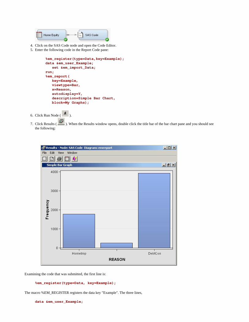
4. Click on the SAS Code node and open the Code Editor.5. Enter the following code in the Report Code pane:

%em_register(type=Data,key=Example);data &em_user_Example; set &em_import_Data;run;%em_report( key=Example, viewtype=Bar, x=Reason, autodisplay=Y, description=Simple Bar Chart, block=My Graphs);

6. Click Run Node ( ).

7. Click Results ( ). When the Results window opens, double click the title bar of the bar chart pane and you should see the following:

Examining the code that was submitted, the first line is:

%em_register(type=Data, key=Example);

The macro %EM_REGISTER registers the data key "Example". The three lines,

data &em_user_Example;

set &em_import_Data;run;

performs a SAS data step. By using the macro variable &em_user_Example for the data set name, the data set name is linked to the data key that was registered previously. So the general form of this macro variable is &em_user_<key>, where <key> is the argument that you supplied to %EM_REGISTER. The macro variable &EM_IMPORT_DATA used in the set statement resolves to the data set that is imported from the Home Equity data node that precedes the SAS Code node in the path. Finally, let's analyze the arguments that were supplied to the macro %EM_REPORT:

%em_report( key=Example, viewtype=Bar, x=Reason, autodisplay=Y, description=Simple Bar Chart, block=My Graphs);

Six arguments were specified. The 1st argument, KEY=Example, links the graph to the data set via the key that was registered previously using %EM_REGISTER; it is a required argument for %EM_REPORT. The 2nd argument, VIEWTYPE=Bar, specifies that a bar chart is the desired type of graph. The 3rd argument, X=Reason, specifies that the variable REASON is to populate the x-axis. By default, the y-axis is the frequency of the variable populating the x-axis, but as will be demonstrated later, this feature of the graph can be changed using the FREQ argument. The variable, Reason, records the reported purpose for the applicant's home equity loan. The 4th argument, AUTODISPLAY=Y, specifies to automatically display the graph in the Results window. Without this option, you would have to use the Results window's View menu to display the graph. The 5th argument, DESCRIPTION=Simple Bar Chart, specifies the text that is to appear in the title bar of the graph pane. The description is also used to populate a View submenu. By default, the View menu will list an item, known as a block, called Custom Reports. The description will be listed in the block's submenu. By including the final option, BLOCK=My Graphs, the block will be labeled "My Graphs" rather than "Custom Reports" and the Description, "Simple Bar Chart" will appear as a menu item under My Graphs.

Our data set includes a variable, JOB, which records the profession of the loan applicant. Suppose you want to see how the frequencies for REASON are distributed across JOB. You can do this by specifying the GROUP option of %EM_REPORT. So, replace the call to %EM_REPORT in your code with the following:

%em_report( key=Example, viewtype=Bar, x=Reason, group=Job, autodisplay=Y, description=REASON grouped by JOB, block=My Graphs);

Save your modified code, click Run Node ( ), and then click Results ( ). You new graph should look like this:

There is a variable in our data set called LOAN that records the dollar amount of the requested loan. Suppose now that instead of displaying the number of loans by type, you want to display the dollar amounts, still grouping by JOB. To do this, add the FREQ argument to %EM_REPORT. Replace the call to %EM_REPORT with the following:

%em_report( key=example, viewtype=Bar, x=Reason, group=Job, freq=Loan, autodisplay=Y, description=REASON grouped by JOB weighted by LOAN, block=My Graphs);

Save your modified code, click Run Node ( ), and then click Results ( ). You new graph should look like this:

Multiple Bar Charts

The previous example, Bar Charts, demonstrated how to generate a single bar chart using %EM_REPORT. Specifically, using the Home Equity data set, a bar chart was generated for the variable REASON, grouped by JOB, and weighted by LOAN. This example extends that example by demonstrating how to generate a combo box that enables you to view different frames of a plot. The example will start where the previous example finished and will add two additional plots; a different weight variable will be used for each frame of the plot. This is accomplished by including the VIEW argument of %EM_REPORT to specify an ID value in multiple calls to %EM_REPORT. The CHOICETEXT argument is also used, enabling you to attach text to each frame that is displayed by the combo box.



%em_register(type=Data, key=Example);data &em_user_Example;set &em_import_data;run; %em_report( key=Example, viewtype=Bar, view=1, x=Reason, group=Job, freq=Loan,

choicetext=Loan, autodisplay=Y, description=Reason by Job with Weights, block=My Graphs);

%em_report( view=1, freq=Value, choicetext=Value); %em_report( view=1, freq=Mortdue, choicetext=Mortdue);

Each call to %EM_REPORT defines a different frame for the graph. There are three things you should notice about the second and third calls to %EM_REPORT. The first is that you must specify the VIEW argument with the same ID number in all three calls to %EM_REPORT. This links the three calls. The second is that except for the VIEW argument, the only other arguments that you need to specify are the ones that have values that differ from the first call to %EM_REPORT. The third is that while arguments can have different values across the multiple calls to %EM_REPORT, you cannot specify different sets of arguments.



Click on the drop-down arrow to choose a different frame to view.

There is no pre-defined limit on the number of frames that you can have. However, as the number of frames grows large, the utility of the combo box declines.

Multiple Y Plot

This example demonstrates how to use the macro %EM_REPORT to generate a line plot with two variables on the y-axis. The technique demonstrated previously, in the example Multiple Bar Charts, for generating multiple frames will also be applied.

1. Create a new diagram2. Add a SAS Code node to the diagram. The data for the example will be simulated.3. Click on the SAS Code node and open the Code Editor.4. Enter the following code in the Report Code pane:

%em_register(type=Data, key=Sample);

/* Simulate the data */

data &em_user_Sample; do X=1 to 100; var1 = 10 + ranuni(1234)*2; var2 = 10 + rannor(1234)*2; var3 = 10 + rannor(1234)*2.5; output; end;run ;

%em_report( key=Sample, viewtype=Lineplot, view=2, x=X, /* specify the x-axis variable */ y1=var1, /* specify the 1st y-axis variable */ y2=var2, /* specify the 2nd y-axis variable */ choicetext=FirstFrame, autodisplay=Y, description= Line Plots, block=My Graphs);

%em_report( view=2, y1=var2, y2=var3, choicetext=SecondFrame);



Click the drop-down arrow and select SecondFrame:

%EM_REPORT allows you to overlay up to16 variables on the y-axis using the Y1=<variable name>, Y2=<variable name>, ... , Y16=<variable name> arguments.

Dendrogram

This example demonstrates how to use the macro %EM_REPORT to generate a dendrogram.


4. Click on the SAS Code node and open the Code Editor5. Enter the following code in the Report Code pane:

%em_register(key=Outtree, type=Data);%em_getname(key=Outtree, type=Data);proc varclus data = &em_import_data hi outtree=&em_user_Outtree;var Clage Clno Debtinc Delinq Derog Loan Mortdue Ninq Value Yoj;run;%em_report( key=OUTTREE, viewtype=DENDROGRAM, autodisplay=Y, block=Dendrogram, name=_Name_, parent=_Parent_, height=_Varexp_);

Note: The macro %EM_GETNAME used in the example code above returns a filename an initializes the macro variable &EM_USER_KEY, where KEY is the data key defined in the call to %EM_REGISTER.


7. Click Results ( ). When the Results window opens, close the output pane and double click the title bar of the OUTTREE pane and you should see the following:

If you click on View in the Results window you will see the item Dendrogram; it will have a submenu item, OUTTREE.

Three Dimensional Components

This example demonstrates how to use %EM_REPORT to generate 3-dimensional scatter, bar, and surface plots.

1. Create a new diagram2. Add a SAS Code node to the diagram. The example uses simulated data and data that is available from the SASHELP

library that is automatically included with your SAS installation.3. Click on the SAS Code node and open the Code Editor.4. Enter the following code in the Report Code pane:

%em_register(key=Data, type=Data);

/* simulate data */

data One;do i = 1 to 100; x= ranuni(0) * 100 * 200; y = ranuni(0) * 100 + 75; z = ranuni(0) * 100 + 10; output; end;run;

data &em_user_data; set Work.One;run;

/* K-Dimensional Scatter Plot */

%em_report( key=Data, viewtype=ThreeDScatter,

x=X, y=Y, z=Z, block=My Graphs, description=3DScatterPlot, autodisplay=Y);

/* K-Dimensional Surface Plot */

%em_report( key=Data, viewtype=Surface, x=X, y=Y, z=Z, block=My Graphs, description=Surface, autodisplay=Y);

%em_register(key=Class, type=Data);

data &em_user_Class; set Sashelp.Class;run;

/* K-Dimensional Bar Chart */

%em_report( key=Class, viewtype=ThreeDBar, x=Name, y=Weight, series=Age, block=My Graphs, description=3DBar, autodisplay=Y);


6. Click Results ( ).

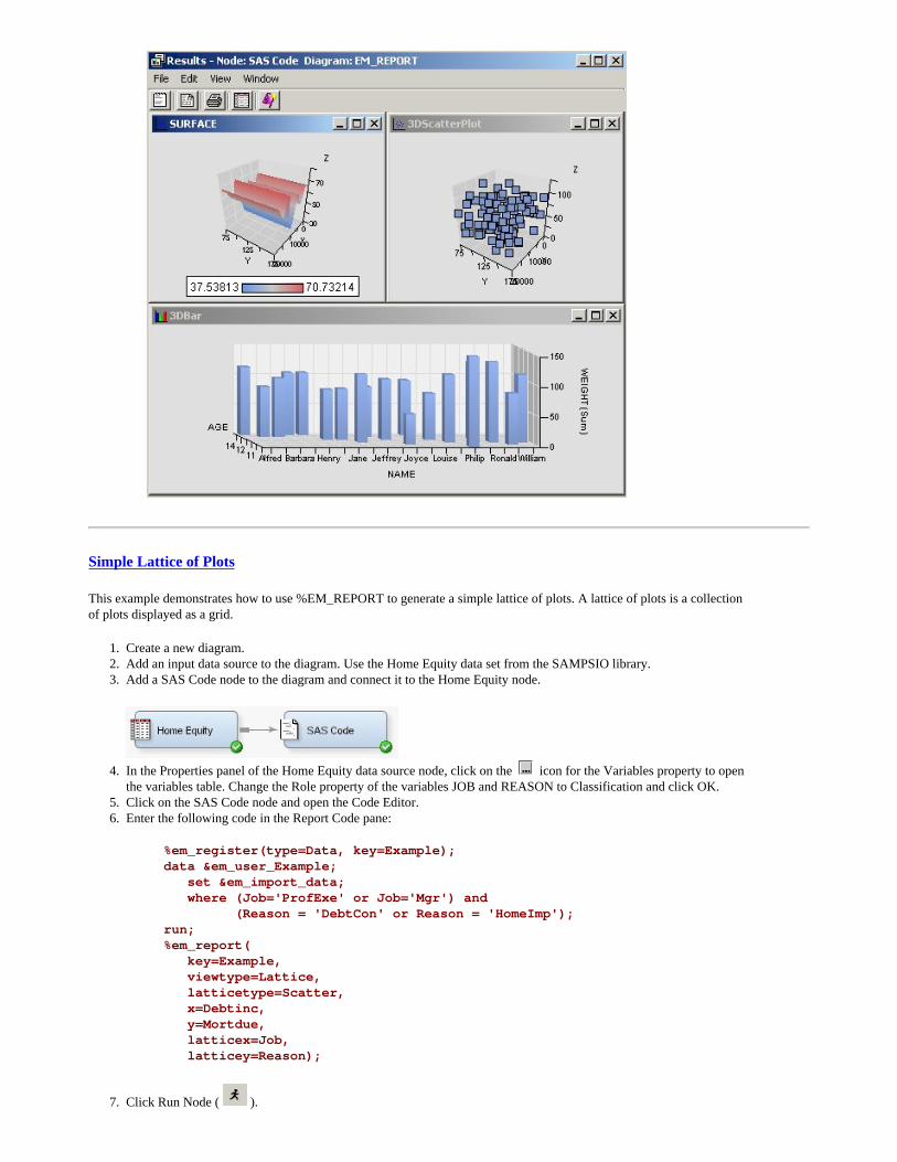
Simple Lattice of Plots

This example demonstrates how to use %EM_REPORT to generate a simple lattice of plots. A lattice of plots is a collection of plots displayed as a grid.

1. Create a new diagram.2. Add an input data source to the diagram. Use the Home Equity data set from the SAMPSIO library.3. Add a SAS Code node to the diagram and connect it to the Home Equity node.

4. In the Properties panel of the Home Equity data source node, click on the icon for the Variables property to open

the variables table. Change the Role property of the variables JOB and REASON to Classification and click OK.5. Click on the SAS Code node and open the Code Editor.6. Enter the following code in the Report Code pane:

%em_register(type=Data, key=Example);data &em_user_Example; set &em_import_data; where (Job='ProfExe' or Job='Mgr') and (Reason = 'DebtCon' or Reason = 'HomeImp');run;%em_report( key=Example, viewtype=Lattice, latticetype=Scatter, x=Debtinc, y=Mortdue, latticex=Job, latticey=Reason);


8. Click Results ( ). When the Results window opens, select View Custom Reports example.

Constellation Plot

This example demonstrates how to use %EM_REPORT to generate a Constellation plot.

1. Create a new diagram.2. Add an input data source to the diagram. Use the Associations data set from the SAMPSIO library.3. Add an Association node to the diagram and connect it to the data source node.4. Add a SAS Code node to the diagram and connect it to the Association node.


%em_register(key=A, type=DATA);%em_register(key=B, type=DATA);

data &em_user_a; set &em_lib..assoc_links;run;

data &em_user_b; set &em_lib..assoc_nodes;run;

%em_report(viewtype=Constellation, linkkey=A, nodekey=B, LINKFROM=FROM, LINKTO=TO, LINKID=linkid, LINKVALUE=CONF, nodeid=item, nodesize=count, nodetip=item);


8. Click Results ( ). When the Results window opens, select View Custom Reports Link Graph.


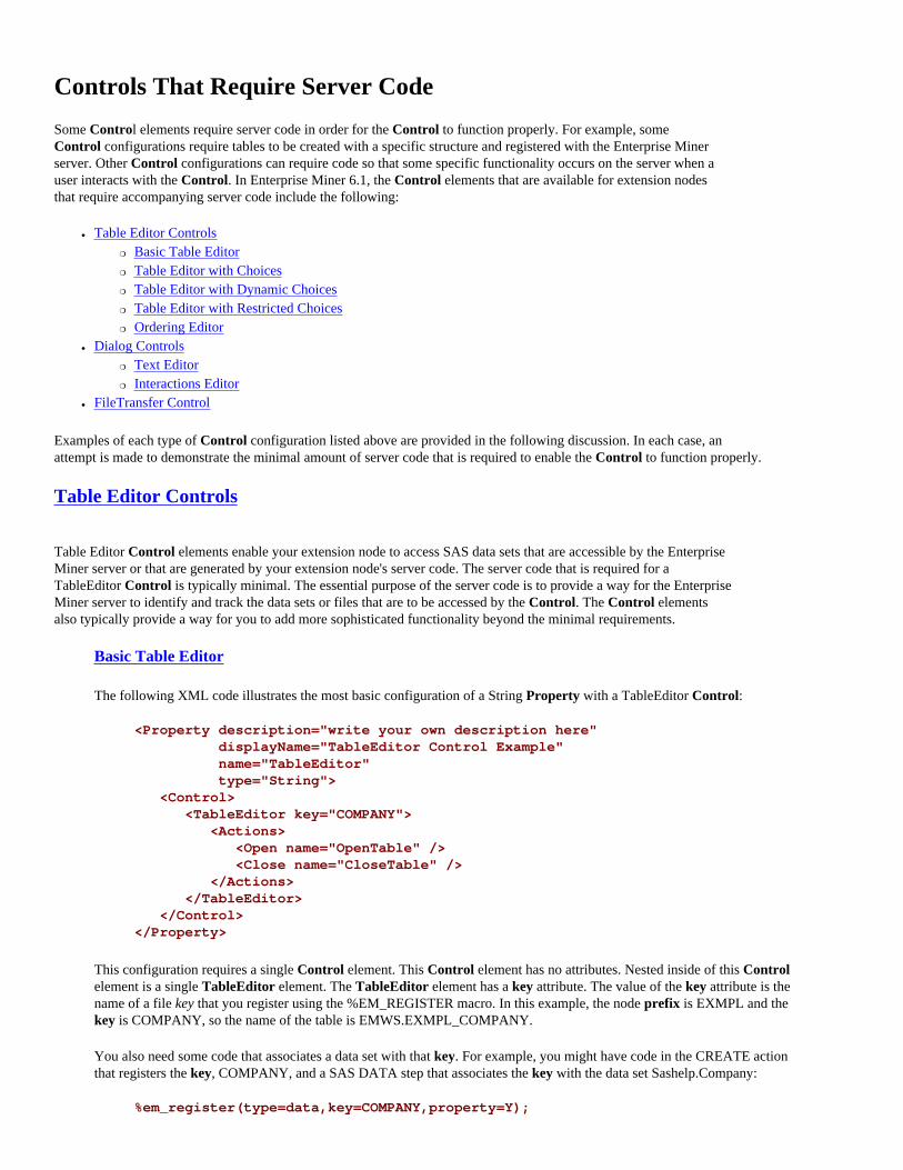
Controls That Require Server CodeSome Control elements require server code in order for the Control to function properly. For example, some Control configurations require tables to be created with a specific structure and registered with the Enterprise Miner server. Other Control configurations can require code so that some specific functionality occurs on the server when a user interacts with the Control. In Enterprise Miner 6.1, the Control elements that are available for extension nodes that require accompanying server code include the following:

● Table Editor Controls �❍ Basic Table Editor�❍ Table Editor with Choices�❍ Table Editor with Dynamic Choices�❍ Table Editor with Restricted Choices�❍ Ordering Editor

● Dialog Controls �❍ Text Editor�❍ Interactions Editor

● FileTransfer Control

Examples of each type of Control configuration listed above are provided in the following discussion. In each case, an attempt is made to demonstrate the minimal amount of server code that is required to enable the Control to function properly.

Table Editor Controls

Table Editor Control elements enable your extension node to access SAS data sets that are accessible by the Enterprise Miner server or that are generated by your extension node's server code. The server code that is required for a TableEditor Control is typically minimal. The essential purpose of the server code is to provide a way for the Enterprise Miner server to identify and track the data sets or files that are to be accessed by the Control. The Control elements also typically provide a way for you to add more sophisticated functionality beyond the minimal requirements.

Basic Table Editor

The following XML code illustrates the most basic configuration of a String Property with a TableEditor Control:

<Property description="write your own description here" displayName="TableEditor Control Example" name="TableEditor" type="String"> <Control> <TableEditor key="COMPANY"> <Actions> <Open name="OpenTable" /> <Close name="CloseTable" /> </Actions> </TableEditor> </Control> </Property>

This configuration requires a single Control element. This Control element has no attributes. Nested inside of this Control element is a single TableEditor element. The TableEditor element has a key attribute. The value of the key attribute is the name of a file key that you register using the %EM_REGISTER macro. In this example, the node prefix is EXMPL and the key is COMPANY, so the name of the table is EMWS.EXMPL_COMPANY.

You also need some code that associates a data set with that key. For example, you might have code in the CREATE action that registers the key, COMPANY, and a SAS DATA step that associates the key with the data set Sashelp.Company:

%em_register(type=data,key=COMPANY,property=Y);

data &EM_USER_COMPANY; set sashelp.company;run;

If you want the table to be available before run time, place the code that associates the data set with the key in the CREATE action. However, in some cases, the table that you are opening with the TableEditor Control is not created until after the node is run. The data set might be created by a process within the TRAIN code. In that case, you could still register the key in your CREATE code, but the code that associates the key with the data set would be in your TRAIN code. If the user attempted to open the table before the node was run, an error message would appear indicating that the table does not exist.

Nested within the TableEditor element is an Actions element. The Actions element associates a block of SAS code with a user action. Inside of the Actions element are an Open element and a Close element; both have a name attribute. In your node's main program, you can add code that might look like this:

%if %upcase(&EM_ACTION) = OPENTABLE %then %do;

filename temp catalog 'sashelp.emext.example_actions.source'; %include temp; filename temp; %OpenTable; %end; %if %upcase(&EM_ACTION) = CLOSETABLE %then %do;

filename temp catalog 'sashelp.emext.example_actions.source'; %include temp; filename temp; %CloseTable; %end;

The values of the name attributes correspond to the names of the actions that are executed when the user either opens or closes the table. The following actions occur when the user opens the table by clicking the ellipsis ( ) icon:

● The &EM_ACTION macro variable is assigned the value of the Open action (for example, OpenTable) before the server code is processed.

● The &EM_TABLE macro variable is initialized; it resolves to the name of the table (for example, EMWS.EXMPL_COMPANY).

● The OpenTable action that is specified in the Open element executes before a copy of the table is returned to the client.

● A temporary table named WORK.key is created (for example, WORK.COMPANY). This table stores any changes that the user makes to the original table.

The following actions occur when the user closes the table:

● The %EM_ACTION macro variable is assigned the value of the Close action (for example, CloseTable) before the server code is processed.

● The &EM_TABLE macro variable is initialized; it resolves to the name of the table (for example, EMWS.EXMPL_COMPANY).

● The &EM_TEMPTABLE macro variable is initialized; it resolves to the name of the temporary table that contains any changes to the table that the user made (for example, WORK.COMPANY).

● The CloseTable action that is specified in the Close element executes. ● The permanent table is overwritten by the temporary table so that any changes made by the user are recorded in the

permanent table.

You must have at least one named action (Open or Close) specified in the XML properties file for a TableEditor Control. However, you are not required to write any code or to include a call to the action in your main program. When you do not have any code that you want to execute when the table is opened or closed, the Actions, Open, and Close elements act as placeholders.

When implemented, the icon appears in the Value column of the Properties panel.

When a user clicks the icon, a SAS Table Editor window opens, displaying the table that is associated with the Control.

In this example, the entire table is displayed when the user clicks the icon and the table cannot be edited. Adding a Columns element with nested Column elements enables you to control which variables appear in the table and whether a variable's values can be edited by the user. In the following example, the Control configuration restricts which variables are displayed in the table and enables the user to edit the values of those variables:

<Property description="write your own description here" displayName="TableEditor Control Example" name="TableEditor" type="String"> <Control> <TableEditor key="COMPANY"> <Actions> <Open name="OpenTable"/> <Close name="CloseTable"/> </Actions> <Columns displayAll="N"> <Column name="DEPTHEAD" type="String" editable="Y"/> <Column name="JOB1" type="String" editable="Y"/> <Column name="LEVEL3" type="String" editable="Y"/> <Column name="N" type="int" editable="Y"/> <Column name="LEVEL4" type="String" editable="Y"/> </Columns> </TableEditor> </Control> </Property>

In the Columns element, the displayAll attribute has a value of N. This indicates that only those variables that are specifically identified by Column elements should appear when the table is opened. Four Column elements are specified. In each Column element, there are three attributes defined as follows:

● name — specifies the name of the variable to display.● type — specifies one of four supported types of variables. The supported types are as follows:

�❍ boolean�❍ String�❍ int�❍ double

Note: These values are case-sensitive.

● editable — indicates whether the user can modify the variable's values. Valid values are Y or N.

When the editable attribute of a Column element is set to Y, the user can edit the values of the corresponding variable by typing a new value in the SAS Table Editor window.

You can also add Range Control elements to restrict the values that can be used to edit the values in the table. For example, suppose you add a Range Control to the N Column element as follows:

<Property description="write your own description here" displayName="TableEditor Control Example" name="TableEditor" type="String"> <Control> <TableEditor key="COMPANY"> <Actions> <Open name="OpenTable" /> <Close name="CloseTable" /> </Actions> <Columns displayAll="N"> <Column name="DEPTHEAD" type="String" editable="Y"> </Column> <Column name="JOB1" type="String" editable="Y"/> <Column name="LEVEL3" type="String" editable="Y"/> <Column name="LEVEL4" type="String"

editable="Y"/> <Column name="N" type="int" editable="Y"> <Control> <Range min="1" max="3" /> </Control> </Column> </Columns> </TableEditor> </Control> </Property>

Now when the user tries to edit the N column of the table, they must enter an integer value between the min and max values specified. If they enter a value that is outside of that range, the value of N is set to missing in that row of the table.

Table Editor with Choices

You can also add a ChoiceList Control to restrict the values that can be used to edit the values in the table. For example, suppose you add a ChoiceList Control to the DEPTHEAD Column element as follows:

<Property description="write your own description here" displayName="TableEditor Control Example" name="TableEditor" type="String"> <Control> <TableEditor key="COMPANY"> <Actions> <Open name="OpenTable" /> <Close name="CloseTable" /> </Actions> <Columns displayAll="N"> <Column name="DEPTHEAD" type="String" editable="Y"> <Control> <ChoiceList> <Choice displayValue="1" rawValue="1"/> <Choice displayValue="2" rawValue="2"/> </ChoiceList> </Control> </Column> <Column name="JOB1" type="String" editable="Y"/> <Column name="LEVEL3" type="String" editable="Y"/> <Column name="LEVEL3" type="String" editable="Y"/> <Column name="N" type="int" editable="Y"> <Control> <Range min="1" max="3" /> </Control> </Column> </Columns> </TableEditor> </Control> </Property>

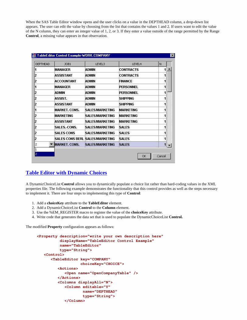
When the SAS Table Editor window opens and the user clicks on a value in the DEPTHEAD column, a drop-down list appears. The user can edit the value by choosing from the list that contains the values 1 and 2. If users want to edit the value of the N column, they can enter an integer value of 1, 2, or 3. If they enter a value outside of the range permitted by the Range Control, a missing value appears in that observation.

Table Editor with Dynamic Choices

A DynamicChoiceList Control allows you to dynamically populate a choice list rather than hard-coding values in the XML properties file. The following example demonstrates the functionality that this control provides as well as the steps necessary to implement it. There are four steps to implementing this type of Control:

1. Add a choiceKey attribute to the TableEditor element.2. Add a DynamicChoiceList Control to the Column element.3. Use the %EM_REGISTER macro to register the value of the choiceKey attribute.4. Write code that generates the data set that is used to populate the DynamicChoiceList Control.

The modified Property configuration appears as follows:

<Property description="write your own description here" displayName="TableEditor Control Example" name="TableEditor" type="String"> <Control> <TableEditor key="COMPANY" choiceKey="CHOICE"> <Actions> <Open name="OpenCompanyTable" /> </Actions> <Columns displayAll="N"> <Column editable="Y" name="DEPTHEAD" type="String"> </Column>

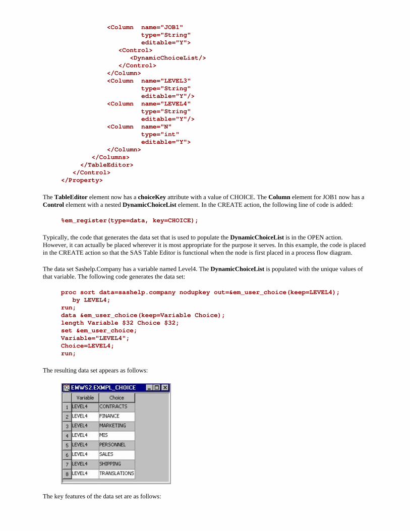
<Column name="JOB1" type="String" editable="Y"> <Control> <DynamicChoiceList/> </Control> </Column> <Column name="LEVEL3" type="String" editable="Y"/> <Column name="LEVEL4" type="String" editable="Y"/> <Column name="N" type="int" editable="Y"> </Column> </Columns> </TableEditor> </Control> </Property>

The TableEditor element now has a choiceKey attribute with a value of CHOICE. The Column element for JOB1 now has a Control element with a nested DynamicChoiceList element. In the CREATE action, the following line of code is added:

%em_register(type=data, key=CHOICE);

Typically, the code that generates the data set that is used to populate the DynamicChoiceList is in the OPEN action. However, it can actually be placed wherever it is most appropriate for the purpose it serves. In this example, the code is placed in the CREATE action so that the SAS Table Editor is functional when the node is first placed in a process flow diagram.

The data set Sashelp.Company has a variable named Level4. The DynamicChoiceList is populated with the unique values of that variable. The following code generates the data set:

proc sort data=sashelp.company nodupkey out=&em_user_choice(keep=LEVEL4); by LEVEL4;run;data &em_user_choice(keep=Variable Choice);length Variable $32 Choice $32;set &em_user_choice;Variable="LEVEL4";Choice=LEVEL4;run;

The resulting data set appears as follows:

The key features of the data set are as follows:

● The name of the data set is contained in the macro variable &EM_USER_choiceKey, where choiceKey is the value of the choiceKey attribute of the TableEditor element.

● The data set has exactly two character variables: Variable and Choice.● Each record of the data set has a value of LEVEL4 in the variable named Variable. LEVEL4 is the value of the name

attribute of the Column element to which the DynamicChoiceList element is applied.● Each record contains a unique value in the Choice variable. These unique values are the choices that populate the

DynamicChoiceList.

In this example, the NODUPKEY option of the SORT procedure ensures that the values are unique.

The DynamicChoiceList element can be applied to multiple Column elements in a TableEditor Control. In such a case, the data set has a repeated measures structure. That is, imagine that there are k Column elements to which you want to apply a DynamicChoiceList. You still create one data set to populate the k lists. The data set has the following structure:

Variable Choice

variable-name_1 value 1_1variable-name_1 value 1_2variable-name_1 ...variable-name_1 value 1_N1variable-name_2 value 2_1variable-name_2 value 2_2variable-name_2 ...variable-name_2 value 2_N2 . . . . . . variable-name_k value k_1variable-name_k value k_2variable-name_k ...variable-name_k value k_Nk

In this example, when the Table Editor window is opened, the user can modify the value for LEVEL4 in any observation by selecting from the list of values that already exist in the data set.

You can provide some additional control over how the data is displayed in the SAS Table Editor window by adding whereClause and whereColumn attributes to the TableEditor element. For example, change the TableEditor element as follows:

<TableEditor key="COMPANY" choiceKey="CHOICE" whereClause="Y" whereColumn="DEPTHEAD">

The whereClause attribute is redundant, but it is required; it should have a value of Y. The whereColumn specifies the name of a variable in the data set. Including these two attributes sorts the data set by the values of the variable specified in the whereColumn attribute. A drop-down list is added at the top of the SAS Table Editor window. The values in the list correspond to the unique values of the variable specified in the whereColumn attribute and the additional value of All. By default, only observations with a value corresponding to the first value in the list are displayed. The user can then select a different value from the drop-down list; the table is refreshed and the observations that correspond to the new value are displayed. If the user selects All, the entire table is displayed.

Table Editor with Restricted Choices

In the example above, the choices for the variable Level4 were populated using a DynamicChoiceList Control. By adding a single new attribute and modifying the accompanying SAS code, you can take advantage of the hierarchical structure of the SASHelp.Company data set to restrict the values that are used to populate the choices. For example, consider the following modified Property configuration:

<Property description="write your own description here" displayName="TableEditor Control Example" name="TableEditor" type="String"> <Control> <TableEditor key="COMPANY" choiceKey="CHOICE" keyVar="LEVEL3" whereClause="Y" whereColumn="DEPTHEAD"> <Actions> <Open name="OpenCompanyTable" /> <Close name="CloseCompanyTable" /> </Actions> <Columns displayAll="N"> <Column editable="Y" name="DEPTHEAD" type="String"/> <Column name="JOB1" type="String" editable="Y"/> <Column name="LEVEL3" type="String" editable="Y"/> <Column name="LEVEL4" type="String" editable="Y"> <Control> <DynamicChoiceList/>

</Control> </Column> <Column name="N" type="int" editable="Y"/> </Columns> </TableEditor> </Control> </Property>

The essential addition to this configuration is the keyVar attribute of the TableEditor Control. In this example, the keyVar attribute is assigned the value of "LEVEL3". This means that when the choices for the variable LEVEL4 are presented for a given row in the table, the choices are conditional on the value of LEVEL3 in the same row of the table. To accomplish this, a table with a hierarchical structure of choices must be generated as follows:

%em_register(type=data, key=CHOICE) proc sort data=sashelp.company nodupkey out=&em_user_choice(keep= LEVEL3 LEVEL4); by LEVEL3 LEVEL4; run; data &em_user_choice(keep=Variable Choice key); length Variable $32 Choice $32 key $32; set &em_user_choice; Variable="LEVEL4"; Choice=LEVEL4; key=LEVEL3; run;

The resulting data set appears as follows:

The key features of the data set are as follows:

● The name of the data set is contained in the macro variable &EM_USER_choiceKey, where choiceKey is the value of the choiceKey attribute of the TableEditor element.

● The data set has exactly three character variables: Variable, Choice, and key.● Each record of the data set has a value of LEVEL4 in the variable named Variable. LEVEL4 is the value of the name

attribute of the Column element to which the DynamicChoiceList is applied.● The data set has a hierarchical structure with the Choice variable nested within the key variable. Therefore, each record

contains a unique combination of the key and Choice variables. These unique values are the choices that populate the DynamicChoiceList.

In this example, when the user clicks on the variable Level4 in a row where the variable Level3 is "ADMIN" they are presented with one set of choices:

However, when the user clicks on the variable Level4 in a row where the variable Level3 is "SALES/MARKETING" they are presented with a different set of choices:

Ordering Editor

An Ordering Editor provides a means by which you can display a table to the user and enable the user to change the order of the variables in the table. A simple example of an ordering editor's XML Property configuration is as follows:

<Property description="write your own description here" displayName="Ordering Editor Control Example" name="OrderingEditor" type="String"> <Control> <TableEditor key="ORDER" isOrderingEditor="Y"> <Actions> <Open name="OpenOrderTable" /> <Close name="CloseOrderTable" /> </Actions>

<Columns displayAll="Y"> <Column editable="N" name="NAME" type="String"/> </Columns> </TableEditor> </Control> </Property>

Notice the two attributes of the TableEditor Control: key and isOrderingEditor. Just as in the other TableEditor Control example, the value of the key attribute must be registered with Enterprise Miner using the %EM_REGISTER macro in your extension node's server code. The isOrderingEditor attribute tells Enterprise Miner that this table editor is, in fact, an ordering editor.

As with other table editors, an ordering editor requires an Actions element and at least one named action nested within it. However, the named action need not have any server code associated with it. You control which variables appear in the table with the Columns element and the nested Column elements. You can have as many columns in the table as you want.

An ordering editor requires minimal server code to make it functional. All that is really required is that you have a table and that the table be registered. For example, you might have server code in the create action that appears as follows:

%em_register(type=data, key=ORDER); proc contents data=sashelp.company out=&em_user_order(KEEP=NAME);run;

When the user opens the table editor the following table appears. The user can select a variable on the left and use the arrows on the right to move the variable to a higher or lower position in the order.

After the user clicks OK and the table is closed, a new version of the table is stored in the EMWS library under the name prefix_key. In this example the prefix is EXMPL and the key is ORDER, so the newly ordered table is stored in Emws.Exmpl_Order.

Dialog Controls

There are two Dialog Control elements that require server code: the Text Editor and Interactions Editor. Examples for both are presented below.

Text Editor

The most common example of a text editor Dialog Control is the Notes editor that is common to all SAS distributed nodes. The notes editor simply provides a text file in which the user might type notes related to a particular node in a particular process flow diagram. This capability has now been extended to extension nodes in Enterprise Miner 6.1. The XML Property configuration for a Property with a text editor Dialog Control is as follows:

<Property description="Example of a text editor which enables you to enter and modify text in an external file." displayName="Text Editor" name="Code" type="String"> <Control> <Dialog showValue="N" allowTyping="Y" class="com.sas.analytics.eminer.visuals.CodeNodeScoreCodeEditor"> <Option name="key" value="CODE"/> </Dialog> </Control></Property>

First, notice the class attribute of the Dialog element. You must copy that value verbatim. Second , notice the Option element. The Option element has two attributes: name and value. The name attribute has a value of "key" and the value attribute has a value of "CODE". This is simply a different syntax for declaring that this Dialog Control has a key="CODE". The explanation for why the syntax for this type of control is different from all the other controls that have a key attribute is beyond the scope of this discussion.

To register the key for this Dialog Control you use the following syntax in your server code:

%em_register(key=CODE, type=FILE, extension=sas, property=Y);

Registering the key this way informs Enterprise Miner that the text that the user enters into the editor is to be stored in a file named CODE.sas. When property="Y", the contents of the editor get copied along if you use a cut-and-paste action to make a copy of the node. When property="N", the contents of the editor are not preserved if you use a cut-and-paste action to make a copy of the node. No other server code is required for this type of Dialog Control.

When the user clicks on the icon next to the text editor property, the following window appears:

The user can then type any text they want in the editor. When the user clicks OK, the file is saved under the name CODE.sas in the extension node's directory for that particular process flow diagram. For example, if the projects directory is c:\emprojects and the project name is "extension nodes", then CODE.sas is created in c:\emprojects\extension nodes\Workspaces\EMWS\EXMPL.

Interactions Editor

When developing statistical models, it is common to include interactions between explanatory variables in your model. For

example, if you have the variables A and B, their interaction is written A*B. An interaction editor provides a way for a user to manually construct a collection of interactions that can be used by your extension node.

The XML Property configuration for a Property with an interactions editor Dialog Control is as follows:

<Property type="String" name="Interaction" displayName="Interactions Editor" description="Example of an Interaction Editor."> <Control> <Dialog showValue="N" allowTyping="N" class="com.sas.analytics.eminer.visuals.InteractionsEditorDialog" > <Option name="Key" value="INTERACTION"/> <Option name="MainEffect" value="N"/> <Option name="MaxTerms" value="2"/> <Option name="Open" value="openInteractionTable"/> <Option name="Close" value="closeInteractionTable"/> <Option name="IntervalVariable" value="N"/> </Dialog> </Control></Property>

The class attribute of the Dialog element uniquely distinguishes this Dialog Control from the other type of Dialog Control elements and must be copied verbatim. Each of the Option elements has two attributes: name and value. These Option elements and their attributes determine the interactions editor's capabilities.

The first Option element has a name attribute of "key" and the value attribute has a value of "INTERACTION". This is simply a different syntax for declaring that this Dialog Control has a key="INTERACTION". The explanation for why the syntax for this type of control is different from all the other controls that have a key attribute is beyond the scope of this discussion.

In the second Option element, name="MainEffect" and value="N". This indicates that the interactions editor is not to create an interaction that consists of just a main effect. That is, all interactions must include at least two terms. If value="Y", then an interaction can consist of a main effect. That is, an interaction can consist of a single term.

In the third Option element, name="MaxTerms" and value="2". This indicates that the maximum number of terms that can be included in an interaction is 2. The value attribute can have a range between 2 and 6.

The third and fourth Option elements represent an alternative syntax for the Actions elements that appeared in other Control elements. You must have at least one of these Option elements. You can write server code that is associated with the name you provide in the value attribute of these Option elements, but it is optional. The explanation for why the syntax for this type of control is different from all the other controls that have Actions elements is beyond the scope of this discussion.

In the final Option element, name="IntervalVariable" and value="N". This indicates that interval variables should not be used to populate the list of variables from which the interactions are generated. When value="Y", then interval variables can be included in the list.

The server code that is required for this Dialog Control consists of the following:

%em_register(key=INTERACTION, type=DATA);

data &em_user_interaction; length key 8 Term $32; stop;run;

The first line of code registers the key that appears in the first Option element in the example XML above. The DATA step programming generates an empty data set that has two variables: a numeric variable named key and a string variable named Term.

Finally, before the interactions editor can be populated with variable names, there must be a data source node preceding your extension node in the process flow diagram. For example, suppose you have the following process flow diagram:

When the user clicks on the icon next to the interactions editor property the following window appears:

When the user constructs interactions, saves them, and clicks OK, Enterprise Miner creates the Emws.Exmpl_interaction data set. For example, suppose the user had selected APRTMNT and GENDER for the first interaction, and NTITLE and TELIND for the second interaction, as depicted above. When the user clicks OK, Emws.Exmpl_interaction appears as follows:

The data set ultimately has a hierarchical structure. The value for Key begins at zero for the first interaction and then increments by one for each additional interaction that is generated by the user.

FileTransfer Control

A FileTransfer Control enables a user to select a registered model. Once the user selects a registered model, a collection of data sets and an external file are generated. These data sets and external file provide you with access to information about the registered model. The XML syntax for this Property and Control configuration is as follows:

<Property type="String" name="ModelSelector" displayName="Model Selector" description="Dialog to select a registered model."> <Control> <FileTransfer action="ImportModel" filename=""/> </Control></Property>

There is a single Control element with a nested FileTransfer element. The FileTransfer element has two attributes: action and filename. Copy the syntax for this Control verbatim.

The following server code is required for a FileTransfer Control. Copy this code verbatim in your extension node's code.

%em_register(key=MODELINFO, type=DATA, property=Y);%em_register(key=MODELINPUT, type=DATA, property=Y); %em_register(key=MODELOUTPUT, type=DATA, property=Y); %em_register(key=MODELSTAT, type=DATA, property=Y); %em_register(key=MODELTRAINING, type=DATA, property=Y); %em_register(key=MODELTARGET, type=DATA, property=Y); %em_register(key=MODELSCORE, type=FILE, extension=sas, property=Y);

When a user clicks on the icon next to the Model Selector property, a dialog box appears that enables them to select a registered model. The name of the registered model then appears in the Value column of the Properties panel next to the Model Selector property. Six SAS data sets and a single external file are created. The SAS data sets are created in the EMWS library for the user's project. The external file is created in the extension node's directory for that particular process flow diagram. For example, if the extension node's prefix is EXMPL, then the following seven data sets and files are created:

● Emws.Exmpl_modelinfo — SAS data set containing metadata for the model● Emws.Exmpl_modelinput — SAS data set containing metadata for the model inputs● Emws.Exmpl_modeloutput — SAS data set containing metadata for the model outputs● Emws.Exmpl_modelstat — SAS data set containing fit statistics for the model● Emws.Exmpl_modeltraining — SAS data set containing metadata for the input data source● Emws.Exmpl_modeltarget — SAS data set containing metadata for the target variable● Modelscore.sas — external file containing the score code of the registered model

Predictive Modeling ● Terminology ● Common Features of Predictive Modeling Nodes

�❍ Table of Common Features �❍ Categorical Variables �❍ Predicted Values and Posterior Probabilities �❍ The Frequency Variable and Weighted Estimation

● Differences among Predictive Modeling Nodes ● Computer Resources● Prior Probabilities ● Decisions ● Decision Thresholds and Profit Charts ● Detecting Rare Classes ● Generalization● Input and Output Data Sets

�❍ Scored Data Sets �❍ Fit Statistics

● Combining Models �❍ Ensembles �❍ Unstable Algorithms

● Scoring New Data ● References

Terminology

Predictive modeling tries to find good rules (models) for guessing (predicting) the values of one or more variables in a data set from the values of other variables in the data set. After a good rule has been found, it can be applied to new data sets (scoring) that may or may not contain the variable(s) that are being predicted. The various methods that find prediction rules go by different names in different areas of research, such as regression, function mapping, classification, discriminant analysis, pattern recognition, concept learning, supervised learning, and so on.

In the present context, prediction does not mean forecasting time series. In time series analysis, an entity is observed repeatedly over time, and past values are used to forecast future values. For the predictive modeling methods in Enterprise Miner, each case in a data set represents a different entity, independent of the other cases in the data set. If the entities in question are, for example, customers, then all of the information pertaining to any one customer must be contained in a single case in the data set. If you have a data set in which each customer is described by multiple cases, you must first rearrange the data to place all of the information regarding any one customer into the same case. It is possible to fit some simple autoregressive models by preprocessing the data using the LAG and DIF functions in the SAS Code node, but Enterprise Miner has no convenient interface for making forecasts.

Enterprise Miner provides a number of tools for predictive modeling. Three of these tools are the Regression node, the Decision Tree node, and the Neural Network node. The methods used in these nodes come from several different areas of research, including statistics, pattern recognition, and machine learning. These different areas use different terminology, so before discussing predictive modeling methods, it will be helpful to clarify the terms used in Enterprise Miner. The following list of terms is in logical, not alphabetical order. A more extensive alphabetical glossary can be found in the Glossary.

Synonym A word having a meaning similar to but not necessarily identical to that of another word in at least one sense.

Case A collection of information regarding one of numerous entities represented in a data set. Synonyms: observation, record, example, pattern, sample, instance, row, vector, pair, tuple, fact.

Variable One of the items of information represented in numeric or character form for each case in a data set. Synonyms: column, feature, attribute, coordinate, measurement.

Target A variable whose value is known in some currently available data, but will be unknown in some future/fresh/operational data set. You want to be able to predict/guess the values of the target variable(s) from other known variables. Synonyms: dependent variable, response, observed values, training values, desired output, correct output, outcome.

Input A variable used to predict/guess the value of the target variable(s). Synonyms: independent variable, predictor, regressor, explanatory variable, carrier, factor, covariate.

Output A variable computed from the inputs as a prediction/guess of the value of the target variable(s) Synonyms: predicted value, estimate, y-hat.

Model A class of formulas or algorithms used to compute outputs from inputs. A statistical model also includes information about the conditional distribution of the targets given the inputs. See also trained model below. Synonyms: architecture (for neural nets), classifier, expert, equation, function.

Weights Numeric values used in a model that are usually unknown or unspecified prior to the analysis. Synonyms: estimated parameters, estimates, regression coefficients, standardized regression coefficients, betas.

Case Weight A nonnegative numeric variable that indicates the importance of each case. There are three kinds of case weights: frequencies, sampling weights, and variance weights. Enterprise Miner supports only frequencies.

Parameters The true or optimal values of the weights or other quantities (such as standard deviations) in a model.

Training The process of computing good values for the weights in a model, or, for tree-based models, choosing good split variables and split values. Synonyms: estimation, fitting, learning, adaptation, induction, growing (trees, that is).

Trained Model A specific formula or algorithm for computing outputs from inputs, with all weights or parameter estimates in the model chosen via a training algorithm from a class of such formulas or algorithms designated by the model. Synonyms: fitted model.

Generalization The ability of a model to compute good outputs from input data not used during training. Synonyms: interpolation and extrapolation, prediction.

Population The set of all cases that you want to be able to generalize to. The data to be analyzed in data mining are usually a subset of the population.

Sample A subset of the population that is available for analysis.

Noise Unpredictable variation, usually in a target variable. For example, if two cases have identical input values but different target values, the variation in those different target values is not predictable from any model using only those inputs, hence that variation is noise. Noise is often assumed to be random, in which case it is inherently unpredictable. Since noise prevents target values from being accurately predicted, the distribution of the noise can be estimated statistically given enough data. Synonym: error.

Signal Predictable variation in a target variable. It is often assumed that target values are the sum of signal and noise, where the signal is a function of the input variables. Synonyms: Function, systematic component.

Training Data Data containing input and target values, used for training to estimate weights or other parameters. Synonyms: Training set, design set.

Test Data Data containing input and target values, not used during training in any way, but instead used to estimate generalization error. Synonyms: Test set (often confused with validation data).

Validation Data Data containing input and target values, used indirectly during training for model selection or early stopping. Synonyms: Validation set (often confused with test data).

Scoring Applying a trained model to data to compute outputs. Synonyms: running (for neural nets), simulating (for neural nets), filtering (for trees), interpolating or extrapolating.

Interpolation Scoring or generalization for cases on or within the convex hull of the training set in the space of the input variables.

Extrapolation Scoring or generalization for cases outside the convex hull of the training set in the space of the input variables.

Operational Data Data to be scored in a practical application, containing inputs but not target values. Scoring operational data is the main purpose of training models in data mining. Synonyms: scoring data.

Categorical Variable

A variable which for all practical purposes has only a limited number of possible values. Synonyms: class variable, label.

Category One of the possible values of a categorical variable. Synonyms: class, level, label.

Class Variable In data mining, pattern recognition, knowledge discovery, neural networks, etc., a class variable means a categorical target variable, and classification means assigning cases to categories of a target variable. In traditional SAS procedures, class variable means simply categorical variable, either an input or a target.

Measurement The process of assigning numbers to things such that the properties of the numbers reflect some attribute of the things.

Measurement Level

One of several different ways in which properties of numbers can reflect attributes of things. The most common measurement levels are nominal, ordinal, interval, log-interval, ratio, and absolute. For details, see the Measurement Theory FAQ at

ftp://ftp.sas.com/pub/neural/measurement.html .

Nominal Variable A numeric or character categorical variable in which the categories are unordered, and the category values convey no additional information beyond category membership.

Ordinal Variable A numeric or character categorical variable in which the categories are ordered, but the category values convey no additional information beyond membership and order. In particular, the number of levels between two categories is not informative, and for numeric variables, the difference between category values is not informative. The results of an analysis that includes ordinal variables will typically be unchanged if you replace all the values of an ordinal variable by different numeric or character values as long as the order is maintained, although some algorithms may use the numeric values for initialization. Enterprise Miner provides no explicit support for continuous ordinal variables, although some procedures in other SAS products do so, such as TRANSREG and PRINQUAL.

Interval Variable A numeric variable for which differences of values are informative.

Ratio Variable A numeric variable for which ratios of values are informative. In Enterprise Miner, ratio and higher-level variables are not generally distinguished from interval variables, since the analytical methods are the same. However, ratio measurements are required for some computations in model assessment, such as profit and ROI measures.

Binary Variable A variable that takes only two distinct values. A binary variable can be legitimately treated as nominal, ordinal, interval, or sometimes ratio.

Common Features of Predictive Modeling Nodes

● Table of Common Features

● Categorical Variables

● Predicted Values and Posterior Probabilities ● The Frequency Variable and Weighted Estimation

Table of Common Features

The predictive modeling nodes are designed to share many common features. The following table lists some features that are broadly applicable to predictive modeling and indicates which nodes have the features. Decision options, output data sets, and score variables are described in subsequent sections of this chapter.

Features of Predictive Modeling Nodes

Neural Network Regression Decision

Tree

Input Data Sets:

Training Yes Yes Yes

Validation Yes Yes Yes

Test Yes Yes Yes

Scoring Yes Yes Yes

Input Variables:

Nominal Yes Yes Yes

Ordinal Yes No# Yes

Interval Yes Yes Yes

Target Variables:

Nominal Yes Yes Yes

Ordinal Yes Yes Yes

Interval Yes Yes Yes

Other Variable Roles:

Frequency Yes Yes Yes

Sampling Weight No* No* No*

Variance Weight No No No

Cost Yes Yes Yes

Decision Options:

Prior Probabilities Yes Yes Yes

Profit or Loss Matrix Yes Yes Yes

Output Data Sets:

Scores Yes Yes Yes

Model (weights, trees) Yes Yes Yes

Fit Statistics Yes Yes Yes

Profit or Loss Summaries Yes Yes Yes

Score Variables:

Output (predicted value, posterior probability)

Yes Yes Yes

Residual Yes Yes Yes

Classify (from, into) Yes Yes Yes

Expected Profit or Loss Yes Yes Yes

Profit or Loss Computed from Target Yes Yes Yes

Decision Yes Yes Yes

Other Features:

Interactive Training Yes No Yes

Save and reuse models Yes Yes Yes

Apply model with missing inputs No No Yes

DATA step code for scoring Yes Yes Yes

# — The Regression node treats ordinal inputs as nominal; it does not preserve the ordering of the levels.

* — Planned for a future release.

Categorical Variables

Categories for nominal and ordinal variables are defined by the normalized, formatted values of the variable. If you have not explicitly assigned a format to a variable, the default format for a numeric variable is BEST12., and the default format for a character variable is $w., where w is the length of the variable. The formatted value is normalized by:

1. Removing leading blanks 2. Truncating to 32 characters 3. Changing lowercase letters to uppercase.

Hence, if two values of a variable differ only in the number of leading blanks and the in the case of their letters, they will be assigned to the same category. Also, if two values differ only past the first 32 characters (after left-justification), they will be assigned to the same category.

Dummy variables are generated for categorical variables in the Regression and Neural Network nodes. If a categorical variable has c categories, the number of dummy variables will be either c or c-1, depending on the role of the variable and what options are specified. The computer time and memory requirements for analyzing a categorical variable with c categories are the same as the requirements for analyzing c or c-1 interval-level variables for the Regression and Neural Network nodes.

When a categorical variable appears in two or more data sets used in the same modeling node, such as the training set (prior to DMDB processing), validation set, and decision data set, the variable is not required to have the same type and length in each data set. For example, a variable named TEMPERAT could be numeric in the training set with values such as 98.6, while a variable by the same name in the validation set could be character with values such as "98.6". As long as the normalized, formatted values from the two data sets agree, the values of the two variables will be matched correctly. In the Neural Network node only, a categorical variable that appears in two or more data sets must have the same formatted length in each data set.

Predicted Values and Posterior Probabilities

For an interval target variable, by default the modeling nodes try to predict the conditional mean of the target given the values of the input variables. The Neural Network node also provides robust error functions that can be used to predict approximately the conditional median or mode of the target.

For a categorical target variable, by default the modeling nodes try to estimate the conditional probability of each class given the values of the input variables. These conditional probabilities are called posterior probabilities. Given the posterior probabilities, each case can be classified into the most probable class.

You can also specify a profit or loss matrix to classify cases according to the business consequences of the decision (see the section below on Decisions). The robust error functions in the Neural Network node can be used to output the approximately most probable class.

When comparing predictive models, it is essential to compare all models using the same cases. If a case is omitted from scoring for one model but not from another (for example, because of missing input variables) you get invalid, "apples-and-oranges" model comparisons. Therefore, Enterprise Miner modeling nodes compute predictions for all cases, even for cases where the model is inapplicable because of missing inputs or other reasons (except, of course, when there are no valid target values).

For cases where the model cannot be applied, the modeling nodes output the unconditional mean (the mean for all cases used for training) for interval targets, or the prior probabilities for categorical targets (see the section below on Prior Probabilities). If you do not specify prior probabilities, implicit priors are used, which are the proportions of the classes among all cases used for training. A variable named _WARN_ in the scored data set indicates why the model could not be applied. If you have lots of cases with missing inputs, you should either use the Decision Tree node for modeling, or use the Impute node to impute missing values prior to using the Regression or Neural Network nodes.

The Frequency Variable and Weighted Estimation

All of the Enterprise Miner modeling nodes allow you to specify a frequency variable. Typically, the values of the frequency variable are nonnegative integers. The data are treated as if each case were replicated as many times as the value of the frequency variable.

Unlike most SAS procedures, the modeling nodes in Enterprise Miner accept values for a frequency variable that are not integers without truncating the fractional part. Thus, you can use a frequency variable to perform weighted analyses.

However, Enterprise Miner does not provide explicit support for sampling weights, noise-variance weights, or other analyses where the weight variable does not represent the frequency of occurrence of each case. If the frequency variable represents sampling weights or noise-variance weights, the point estimates of regression coefficients and neural network weights will be valid. But if the frequency variable does not represent actual frequencies, then standard errors, significance tests, and statistics such as MSE, AIC, and SBC may be invalid.

If you want to do weighted estimation under the usual assumption for weighted least-squares that the weights are inversely proportional to the noise variance (error variance) of the target variable, then you can obtain statistically correct results by specifying frequency values that add up to the sample size.

If you want to use sampling weights that are inversely proportional to the sampling probability of each case, you can get approximate estimates for MSE and related statistics in the Regression and Neural Network nodes by specifying frequencies that add up to the effective sample size. A pessimistic approximation to the effective sample size is provided by

,

where W(i) is a sampling weight for case i. This approximation will not work properly with the Decision Tree node.

Differences Among Predictive Modeling Nodes

The Regression node, the Tree node, and the Neural Network node can all learn complex models from data, but they have different ways of representing complexity in their models. Choosing a model of appropriate complexity is important for making accurate predictions, as discussed in the section below on Generalization. Simple models are best for learning simple functions of the data (as long as the model is correct, of course), while complex models are required for learning complex functions. With all data mining models, one way to increase the complexity of a model is to add input variables. Other ways to increase complexity depend on the type of model:

● In regression models, you can add interactions and polynomial terms. ● In neural networks, you can add hidden units. ● In tree-based models, you can grow a larger tree.

One fundamental difference between tree-based models and both regression and neural net models is that tree-based models learn step functions, whereas the other models learn continuous functions. If you expect the function to be discontinuous, a tree-based model is a good way to start. However, given enough data and training time, neural networks can approximate discontinuities arbitrarily well. Polynomial regression models are not good at learning discontinuities. To model discontinuities using regression, you need to know where the discontinuities occur and construct dummy variables to indicate the discontinuities before fitting the regression model.

For both regression and neural networks, the simplest models are linear functions of the inputs, hence regression and neural nets are both good for learning linear functions. Tree-based models require many branches to approximate linear functions accurately.

When there are many inputs, learning is inherently difficult because of the curse of dimensionality (see the Neural Network FAQ at the URL

ftp://ftp.sas.com/pub/neural/FAQ2.html#A_curse.

To learn general nonlinear functions, all modeling methods require a degree of complexity that grows exponentially with the number of inputs. That is, as the number of inputs increases, the number of interactions and polynomial terms required in a regression model grows exponentially, the number of hidden units required in a neural network grows exponentially, and the number of branches required in a tree grows exponentially. The amount of data and the amount of training time required to learn such models also grow exponentially.

Fortunately, in most practical applications with a large number of inputs, most of the inputs are irrelevant or redundant, and the curse of dimensionality can be circumvented. Tree-based models are especially good at ignoring irrelevant inputs, since trees often use a relatively small number of inputs even when the total number of inputs is large.

If the function to be learned is linear, stepwise regression is good for choosing a small number out of a large set of inputs. For nonlinear models with many inputs, regression is not a good choice unless you have prior knowledge of which interactions and polynomial terms to include in the model. Among various neural net architectures, multilayer perceptrons and normalized radial basis function (RBF) networks are good at ignoring irrelevant inputs and finding relevant subspaces

of the input space, but ordinary radial basis function networks should only be used when all or most of the inputs are relevant.

All of the modeling nodes can process redundant inputs effectively. Adding redundant inputs has little effect on the effective dimensionality of the data; hence the curse of dimensionality does not apply. When there are redundant inputs, the training cases lie close to some (possibly nonlinear) subspace. If this subspace is linear, redundancy is called multicollinearity.

In statistical theory, it is well-known that redundancy causes parameter estimates (weights) to be unstable; that is, different parameter estimates can produce similar predictions. But if the purpose of the analysis is prediction, unstable parameter estimates are not necessarily a problem. If the same redundancy applies to the test cases as to the training cases, the model needs to produce accurate outputs only near the subspace occupied by the data, and stable parameter estimates are not needed for accurate prediction. However, if the test cases do not follow the same pattern of redundancy as the training cases, generalization will require extrapolation and will rarely work well.

If extrapolation is required, decision tree-based models are safest, because trees choose just one of several redundant inputs and produce constant predictions outside the range of the training data. Stepwise linear regression or linear-logistic regression are the next safest methods for extrapolation if a large singularity criterion is used to make sure that the parameter estimates do not become excessively unstable. Polynomial regression is usually a bad choice for extrapolation, because the predictions will often increase or decrease rapidly outside the range of the training data. Neural networks are also dangerous for extrapolation if the weights are large. Weight decay and early stopping can be used to discourage large weights. Normalized radial basis function (RBF) networks are the safest type of neural net architecture for extrapolation, since the range of predictions will never exceed the range of the hidden-to-output weights.

The Decision Tree node can use cases with missing inputs for training and provides several ways of making predictions from cases with missing inputs. The Regression and Neural Network nodes cannot use cases with missing inputs for training; predictions are based on the unconditional mean or prior probabilities (see Predicted Values and Posterior Probabilities).

The Neural Network node can model two or more target variables in the same network. Having multiple targets in the network can be an advantage when there are features common to all the targets; otherwise, it is more efficient to train separate networks. The Regression node and the Decision Tree node process only one target at a time, but the Start Group node can be used to handle multiple targets.

The following figures illustrate the kinds of approximation error that commonly occur with each of the modeling nodes. The noise-free data come from the hill-and-plateau function, which was chosen because it is difficult for typical neural networks to learn. Given sufficient model complexity, all of the modeling nodes can, of course, learn the data accurately. These examples show what happens with insufficient model complexity. The cases in the training set lie on a 21 by 21 grid, while those in the test set are on a 41 by 41 grid.

Computer Resources

The computer time and memory required for an analysis depend on the number of cases, the number of variables, the complexity of the model, and the training algorithm. For many modeling methods, there is a trade-off between time and memory.

For all modeling nodes, memory is required for the operating system, SAS supervisor, and the Enterprise Miner diagram and programs, resulting in an overhead of about 20 to 30 megabytes.

Let:

N be the number of cases.

V be the number of input variables.

I be the number of input terms or units, including dummy variables, intercepts, interactions, and polynomials.

W be the number of weights in a neural network.

O be the number of output units.

D be the average depth of a tree.

R be the number of times the training data are read in logistic regression or neural nets, which depends on the training technique, the termination criteria, the model, and the data. R is typically much larger for neural nets than for logistic regression. In regard to training techniques, R is usually smallest for Newton-Raphson or Levenberg-Marquardt, larger for quasi-Newton, and still larger for conjugate gradients.

S be the number of steps in stepwise regression, or 1 if stepwise regression is not used.

For the Decision Tree node, the minimum additional memory required for an analysis is about 8N bytes. Training will be considerably faster if there is enough RAM to hold the entire data set, which is about 8N(V+1) bytes. If the data will not fit in memory, they must be stored in a utility file. Memory is also required to hold summary statistics for a node, such as means or a contingency table, but this amount is usually much smaller than the amount required for the data.

For the Regression node, the memory required depends on the type of model and on the training technique. For linear regression, memory usage is dominated by the SSCP matrix, which requires 8I2 bytes. For logistic regression, memory usage depends on the training technique as documented in the SAS/OR Technical Report: The NLP Procedure, ranging from about 40I bytes for the conjugate gradient technique to about 8I2 bytes for the Newton-Raphson technique.

For the Neural Network node, memory usage depends on the training technique as documented in the SAS/OR Technical Report: The NLP Procedure. About 40W bytes are needed for the conjugate gradient technique, while 4W2 bytes are needed for the quasi-Newton and Levenberg-Marquardt techniques. For a network with biases and H hidden units in one layer, W = (I+1)H + (H+1)O.

For both logistic regression and neural networks, the conjugate gradient technique, which requires the least memory, must usually read the training data many more times than the Newton-Raphson and Levenberg-Marquardt techniques.

Assuming that the number of training cases is greater than the number of inputs or weights, the time required for training is roughly proportional to:

NI2 for linear regression.

SRNI for logistic regression using conjugate gradients.

SRNI2 for logistic regression using quasi-Newton or Newton-Raphson. Note that R is usually considerably less for these techniques than for conjugate gradients.

DNI for decision tree-based models.

RNW for neural nets using conjugate gradients.

RNW2 for neural nets using quasi-Newton or Levenberg-Marquardt. Note that R is usually considerably less for these techniques than for conjugate gradients.

Prior Probabilities

For a categorical target variable, each modeling node can estimate posterior probabilities for each class, which are defined as the conditional probabilities of the classes given the input variables. By default, the posterior probabilities are based on implicit prior probabilities that are proportional to the frequencies of the classes in the training set. You can specify different prior probabilities via the Target Profile using the Prior Probabilities tab (see the Target Profile chapter). Also, given a previously scored data set containing posterior probabilities, you can compute new posterior probabilities for different priors by using the DECIDE procedure, which reads the prior probabilities from a decision data set.

Prior probabilities should be specified when the sample proportions of the classes in the training set differ substantially from the proportions in the operational data to be scored, either through sampling variation or deliberate bias. For example, when the purpose of the analysis is to detect a rare class, it is a common practice to use a training set in which the rare class is over represented. If no prior probabilities are used, the estimated posterior probabilities for the rare class will be too high. If you specify correct priors, the posterior probabilities will be correctly adjusted no matter what the proportions in the training set are. For more information, see Detecting Rare Classes.

Increasing the prior probability of a class increases the posterior probability of the class, moving the classification boundary for that class so that more cases are classified into the class. Changing the prior will have a more noticeable effect if the original posterior is near 0.5 than if it is near zero or one.

For linear logistic regression and linear normal-theory discriminant analysis, classification boundaries are hyperplanes; increasing the prior for a class moves the hyperplanes for that class farther from the class mean, while decreasing the prior moves the hyperplanes closer to the class mean, but changing the priors does not change the angles of the hyperplanes.

For quadratic logistic regression and quadratic normal-theory discriminant analysis, classification boundaries are quadratic hypersurfaces; increasing the prior for a class moves the boundaries for that class farther from the class mean, while decreasing the prior moves the boundaries closer to the class mean, but changing the priors does not change the shapes of the quadratic surfaces.

To show the effect of changing prior probabilities, the data in the following figure were generated to have three classes, shown as red circles, blue crosses, and green triangles. Each class has 100 training cases with a bivariate normal distribution.

These training data were used to fit a quadratic logistic regression model using the Neural Network engine. Since each class has the same number of training cases, the implicit prior probabilities are equal. In the following figure, the plot on the left shows color-coded posterior probabilities for each class. Bright red areas have a posterior probability near 1.0 for the red circle class, bright blue areas have a posterior probability near 1.0 for the blue cross class, and bright green areas have a posterior probability near 1.0 for the green triangle class. The plot on the right shows the classification results as red, blue, and green regions.

If the prior probability for the red class is increased, the red areas in the plots expand in size as shown in the following figure. The red class has a small variance, so the effect is not widespread. Since the priors for the blue and green classes are still equal, the boundary between blue and green has not changed.

If the prior probability for the blue class is increased, the blue areas in the plots expand in size as shown in the following figure. The blue class has a large variance and has a substantial density extending beyond the high-density red region, so increasing the blue prior causes the red areas to contract dramatically.

If the prior probability for the green class is increased, the green areas in the plots expand as shown in the following figure.

In the literature on data mining, statistics, pattern recognition, and so on, prior probabilities are used for a variety of purposes that are sometimes confusing. In Enterprise Miner, however, the nodes are designed to use prior probabilities in a simple, unambiguous way:

● Prior probabilities are assumed to be estimates of the true proportions of the classes in the operational data to be scored. ● Prior probabilities are not used by default for parameter estimation. This allows you to manipulate the class proportions

in the training set by nonproportional sampling or by a frequency variable in any manner you want. ● If you specify prior probabilities, the posterior probabilities computed by the modeling nodes are always adjusted for the

priors. ● If you specify prior probabilities, the profit and loss summary statistics are always adjusted for priors and therefore

provide valid model comparisons, assuming that you specify valid decision consequences (see the following section on Decisions).

If you do not explicitly specify prior probabilities (or if you specify None for prior probabilities in the target profile), no adjustments for priors are performed by any nodes.

Posterior probabilities are adjusted for priors as follows. Let:

t be an index for target values (classes)

i> be an index for cases

OldPrior(t) be the old prior probability or implicit prior probability for target t

OldPost(i,t) be the posterior probability based on OldPrior(t)

Prior(t) be the new prior probability desired for target t

Post(i,t) be the posterior probability based on Prior(t)

Then:

For classification, each case i is assigned to the class with the greatest posterior probability, that is, the class t for which Post(i,t) is maximized.

Prior probabilities have no effect on estimating parameters in the Regression node, on learning weights in the Neural Network node, or, by default, on growing trees in the Tree node. Prior probabilities do affect classification and decision processing for each case. Hence, if you specify the appropriate options for each node, prior probabilities can affect the choice of models in the Regression node, early stopping in the Neural Network node, and pruning in the Tree node.

Prior probabilities are also used to adjust the relative contribution of each class when computing the total and average profit and loss as described in the section below on Decisions. The adjustment of total and average profit and loss is distinct from the adjustment of posterior probabilities. The latter is used to obtain correct posteriors for individual cases, whereas the former is used to obtain correct summary statistics for the sample. The adjustment of total and average profit and loss is done only if you explicitly specify prior probabilities; the adjustment is not done when the implicit priors based on the training set proportions are used.

Note that the fit statistics such as misclassification rate and mean squared error are not adjusted for prior probabilities. These fit statistics are intended to provide information about the training process under the assumption that you have provided an appropriate training set with appropriate frequencies, hence adjustment for prior probabilities could present a misleading picture of the training results. The profit and loss summary statistics are intended to be used for model selection, and to assess decisions that are made using the model under the assumption that you have provided the appropriate prior probabilities and decision values. Therefore, adjustment for prior probabilities is required for data sets that lack representative class proportions. For more details, see Decisions .

If you specify priors explicitly, Enterprise Miner assumes that the priors that you specify represent the true operational prior probabilities and adjusts the profit and loss summary statistics accordingly. Therefore:

● If you are using profit and loss summary statistics, the class proportions in the validation and test sets need not be the same as in the operational data as long as your priors are correct for the operational data.

● You can use training sets based on different sampling methods or with differently weighted classes (using a frequency variable), and as long as you use the same explicitly specified prior probabilities, the profit and loss summary statistics for the training, validation, and test sets will be comparable across all of those different training conditions.

● If you fit two or more models with different specified priors, the profit and loss summary statistics will not be comparable and should not be used for model selection, since the different summary statistics apply to different operational data sets.

If you do not specify priors, Enterprise Miner assumes that the validation and test sets are representative of the operational data, hence the profit and loss summary statistics are not adjusted for the implicit priors based on the training set proportions. Therefore:

● If the validation and test sets are indeed representative of the operational data, then regardless of whether you specify priors, you can use training sets based on different sampling methods or with differently weighted classes (using a frequency variable), and the profit and loss summary statistics for the validation and test sets will be comparable across all of those different training conditions.

● If the validation and test sets are not representative of the operational data, then the validation statistics may not provide valid model comparisons, and the test-set statistics may not provide valid estimates of generalization accuracy.

If a class has both an old prior and a new prior of zero, then it is omitted from the computations. If a class has a zero old prior, you may not assign it a positive new prior, since that would cause a division by zero. Prior probabilities may not be missing or negative. They must sum to a positive value. If the priors do not sum to one, they are automatically adjusted to do so by dividing each prior by the sum of the priors. A class may have a zero prior probability, but if you use PROC DECIDE to update posterior probabilities, any case having a nonzero posterior corresponding to a zero prior will cause the results for that case to be set to missing values.

To summarize, prior probabilities do not affect:

● Estimating parameters in the Regression node. ● Learning weights in the Neural Network node. ● Growing (as opposed to pruning) trees in the Decision Tree node unless you configure the property Use Prior Probability

in Split Search. ● Residuals, which are based on posteriors before adjustment for priors, except in the Decision Tree node if you choose to

use prior probabilities in the split search. ● Error functions such as deviance or likelihood, except in the Decision Tree node if you choose to use prior probabilities

in the split search. ● Fit statistics such as MSE based on residuals or error functions, except in the Decision Tree node if you choose to use

prior probabilities in the split search.

Prior probabilities do affect:

● Posterior probabilities ● Classification ● Decisions ● Misclassification rate ● Expected profit or loss● Profit and loss summary statistics, including the relative contribution of each class.

Prior probabilities will by default affect the following processes if and only if there are two or more decisions in the decision matrix:

● Choice of models in the Regression node ● Early stopping in the Neural Network node● Pruning trees in the Tree node.

Decisions

Each modeling node can make a decision for each case in a scoring data set, based on numerical consequences specified via a decision matrix and cost variables or cost constants. The decision matrix can specify profit, loss, or revenue. In the GUI, the decision matrix is provided via the Target Profile. With a previously scored data set containing posterior probabilities, decisions can also be made using PROC DECIDE, which reads the decision matrix from a decision data set.

When you use decision processing, the modeling nodes compute summary statistics giving the total and average profit or loss for each model. These profit and loss summary statistics are useful for selecting models. To use these summary statistics for model selection, you must specify numeric consequences for making each decision for each value of the target variable. It is your responsibility to provide reasonable numbers for the decision consequences based on your particular application.

In some applications, the numeric consequences of each decision may not all be known at the time you are training the model. Hence you may want to perform what-if analyses to explore the effects of different decision consequences using the Model Comparison node. In particular, when one of the decisions is to "do nothing," the profit charts in the Model Comparison node provide a convenient way to see the effect of applying different thresholds for the do-nothing decision.

To use profit charts, the do-nothing decision should not be included in the decision matrix; the Model Comparison node will implicitly supply a do-nothing decision when computing the profit charts. When you omit the do-nothing decision from the profit matrix so you can obtain profit charts, you should not use the profit and loss summary statistics for comparing models, since these summary statistics will not incorporate the implicit do-nothing decision. This topic is discussed further in Decision Thresholds and Profit Charts.

The decision matrix contains columns (decision variables) corresponding to each decision, and rows (observations) corresponding to target values. The values of the decision variables represent target-specific consequences, which may be profit, loss, or revenue. These consequences are the same for all cases being scored. A decision data set may contain prior probabilities in addition to the decision matrix.

For a categorical target variable, there should be one row for each class. The value in the decision matrix located at a given row and column specifies the consequence of making the decision corresponding to the column when the target value corresponds to the row. The decision matrix is allowed to contain rows for classes that do not appear in the data being analyzed. For a profit or revenue matrix, the decision is chosen to maximize the expected profit. For a loss matrix, the decision is chosen to minimize the expected loss.

For an interval target variable, each row defines a knot in a piecewise linear spline function. The consequence of making a decision is computed by linear interpolation in the corresponding column of the decision matrix. If the predicted target value is outside the range of knots in the decision matrix, the consequence of a decision is computed by linear extrapolation. Decisions are made to maximize the predicted profit or minimize the predicted loss.

For each decision, there may also be either a cost variable or a numeric cost constant. The values of cost variables represent case-specific consequences, which are always treated as costs. These consequences do not depend on the target values of the cases being scored. Costs are used for computing return on investment as (revenue-cost)/cost.

Cost variables may be specified only if the decision matrix contains revenue, not profit or loss. Hence if revenues and costs are specified, profits are computed as revenue minus cost. If revenues are specified without costs, the costs are assumed to be zero. The interpretation of consequences as profits, losses, revenues, and costs is needed only to compute return on investment. You can specify values in the decision matrix that are target-specific consequences but that may have some practical interpretation other than profit, loss, or revenue. Likewise, you can specify values for the cost variables that are case-specific consequences but that may have some practical interpretation other than costs. If the revenue/cost interpretation is not applicable, the values computed for return on investment may not be meaningful. There are some restrictions on the use of cost variables in the Decision Tree node; see the documentation on the Decision Tree node for more information.

In principle, consequences need not be the sum of target-specific and case-specific terms, but Enterprise Miner does not support such non-additive consequences.

For a categorical target variable, you can use a decision matrix to classify cases by specifying the same number of decisions as classes and having each decision correspond to one class. However, there is no requirement for the number of decisions to equal the number of classes except for ordinal target variables in the Decision Tree node.

For example, suppose there are three classes designated red, blue, and green. For an identity decision matrix, the average profit is equal to the correct-classification rate:

Profit Matrix to Compute the Correct-Classification Rate

Target Value:

Decision:

Red Blue Green

Red 1 0 0

Blue 0 1 0

Green 0 0 1

To obtain the misclassification rate, you can specify a loss matrix with zeros on the diagonal and ones everywhere else:

Loss Matrix to Compute the Misclassification Rate

Target Value:

Decision:

Red Blue Green

Red 0 1 1

Blue 1 0 1

Green 1 1 0

If it is 20 times more important to classify red cases correctly than blue or green cases, you can specify a diagonal profit matrix with a profit of 20 for classifying red cases correctly and a profit of one for classifying blue or green cases correctly:

Profit Matrix for Detecting a Rare (Red) Class

Target Value:

Decision:

Red Blue Green

Red 20 0 0

Blue 0 1 0

Green 0 0 1

When you use a diagonal profit matrix, the decisions depend only on the products of the prior probabilities and the corresponding profits, not on their separate values. Hence, for any given combination of priors and diagonal profit matrix, you can make any change to the priors (other than replacing a zero with a nonzero value) and find a corresponding change to the diagonal profit matrix that leaves the decisions unchanged, even though the expected profit for each case may change.

Similarly, for any given combination of priors and diagonal profit matrix, you can find a set of priors that will yield the same decisions when used with an identity profit matrix. Therefore, using a diagonal profit matrix does not provide you with any power in decision making that could not be achieved with no profit matrix by choosing appropriate priors (although the profit matrix may provide an advantage in interpretability). Furthermore, any two by two decision matrix can be transformed into a diagonal profit matrix as discussed in the following section on Decision Thresholds and Profit Charts.

When the decision matrix is three by three or larger, it may not be possible to diagonalize the profit matrix, and

some nondiagonal profit matrices will produce effects that could not be achieved by manipulating the priors. To show the effect of a nondiagonalizable decision matrix, the data in the upper left plot of the following figure were generated to have three classes, shown as red circles, blue crosses, and green triangles.

Each class has 100 training cases with a bivariate normal distribution. The training data were used to fit a linear logistic regression model using the Neural Network engine. The posterior probabilities are shown in the upper right plot. Classification according to the posterior probabilities yields linear classification boundaries as shown in the lower left plot. Use of a nondiagonalizable decision matrix causes the decision boundaries in the lower right plot to be rotated in comparison with the classification boundaries, and the decision boundaries are curved rather than linear.

Linear Logistic Regression with a Nondiagonal Profit Matrix

The decision matrix that produced the curved decision boundaries is shown in the following table:

Nondiagonal Profit Matrix

Target Value:

Decision:

Red Blue Green

Red 4 0 3

Blue 3 4 0

Green 0 3 4

In each row, the two profit values for misclassification are different, hence it is impossible to diagonalize the matrix by adding a constant to each row. Consider the blue row. The greatest profit is for a correct assignment into blue, but there is also a smaller but still substantial profit for assignment into red. There is no profit for assigning red into blue, so the red/blue decision boundary is moved toward the blue mean in comparison with the classification boundary based on posterior probabilities. The following figure shows the effect of the same nondiagonal profit matrix on a quadratic logistic regression model.

Quadratic Logistic Regression with a Nondiagonal Profit Matrix

For the Neural Network and Regression nodes, a separate decision is made for each case. For the Decision Tree node, a common decision is made for all cases in the same leaf of the tree, so when different cases have different costs, the average cost in the leaf is used in place of the individual costs for each case. That is, the profit equals the revenue minus the average cost among all training cases in the same leaf, hence a single decision is assigned to all cases in the same leaf of a tree.

The decision alternative assigned to a validation, test or scoring case ignores any cost associated with the case. The new data are assumed similar to the training data in cost as well as predictive relations. However, the actual cost values for each case are used for the investment cost, ROI, and quantities that depend on the actual target value.

Decision and cost matrices do not affect:

● Estimating parameters in the Regression node ● Learning weights in the Neural Network node● Growing (as opposed to pruning) trees in the Decision Tree node unless the target is ordinal ● Residuals, which are based on posteriors before adjustment for priors ● Error functions such as deviance or likelihood ● Fit statistics such as MSE based on residuals or error functions ● Posterior probabilities ● Classification ● Misclassification rate.

Decision and cost matrices do affect:

● Growing trees in the Decision Tree node when the target is ordinal ● Decisions ● Expected profit or loss● Profit and loss summary statistics, including the relative contribution of each class.

Decision and cost matrices will by default affect the following processes if and only if there are two or more decisions:

● Choice of models in the Regression node ● Early stopping in the Neural Network node● Pruning trees in the Decision Tree node.

Formulas will be presented first for the Neural Network and Regression nodes. Let:

t be an index for target values (classes)

d be an index for decisions

i be an index for cases

Nd be the number of decisions

Class(t) be the set of indices of cases belonging to target t

Profit(t,d) be the profit for making decision d when the target is t

Loss(t,d) be the loss for making decision d when the target is t

Revenue(t,d)

be the revenue for making decision d when the target is t

Cost(i,d) be the cost for making decision d for case i

Q(i,t,d) be the combined consequences for making decision d when the target is t for case i

Prior(t) be the prior probability for target t

Paw(t) be the prior-adjustment weight for target t

Post(i,t) be the posterior probability of target t for case i

F(i) be the frequency for case i

T(i) be the index of the actual target value for case i

A(i,d) be the expected profit of decision d for case i

B(i) be the best possible profit for case i based on the actual target value

C(i) be the computed profit for case i based on the actual target value

D(i) be the index of the decision chosen by the model for case i

E(i) be the expected profit for case i of the decision chosen by the model

IC(i) be the investment cost for case i for the decision chosen by the model

ROI(i) be the return on investment for case i for the decision chosen by the model.

These quantities are related by the following formulas:

When the target variable is categorical, the expected profit for decision d in case i is:

For each case i, the decision is made by choosing D(i) to be the value of d that maximizes the expected profit:

If two or more decisions are tied for maximum expected profit, the first decision in the user-specified list of decisions is chosen.

The expected profit E(i) is the expected combined consequence for the chosen decision D(i), computed as a weighted average over the target values of the combined consequences, using the posterior probabilities as weights:

The expected loss is the negative of expected profit.

Note that E(i) and D(i) can be computed without knowing the target index T(i). When T(i) is known, two more quantities useful for evaluating the model can also be computed. C(i) is the profit computed from the target value using the decision chosen by the model:

The loss computed from the target value is the negative of C(i). C(i) is the most important variable for assessing and comparing models. The best possible profit for any of the decisions, which is an upper bound for C(i), is:

The best possible loss is the negative of B(i).

When revenue and cost are specified, investment cost is:

And return on investment is:

For an interval target variable, let:

Y(i)

be the actual target value for case i

P(i)

be the predicted target value for case i

K(t)

be the knot value for row tof the decision matrix.

For interval targets, the predicted value is assumed to be accurate enough that no integration over the predictive distribution is required. Define the functions:

Then the decision is made by maximizing the expected profit:

The expected profit for the chosen decision is:

When Y(i) is known, the profit computed from the target value using the decision chosen by the model is:

And the best possible profit for any of the decisions is:

For both categorical and interval targets, the summary statistics for decision processing with profit and revenue matrices are computed by summation over cases with nonmissing cost values. If no adjustment for prior probabilities is used, the sums are weighted only by the case frequencies, hence total profit and average profit are given by the following formulas:

For loss matrices, total loss and average loss are the negatives of total profit and average profit, respectively.

If total and average profit are adjusted for prior probabilities, an additional weight Paw(t)is used:

Total and average profit are then given by:

If any class with a positive prior probability has a total frequency of zero, total and average profit and loss cannot be computed and are assigned missing values. Note that the adjustment of total and average profit and loss is done only if you explicitly specify prior probabilities; the adjustment is not done when the implicit priors based on the training set proportions are used.

The adjustment for prior probabilities is not done for fit statistics such as SSE, deviance, likelihood, or misclassification rate. For example, consider the situation shown in the following table:

Proportion in: Unconditional

Misclassification Rate

Class Operational Data

Training Data

Prior Probability

Conditional Misclassification

RateUnadjusted Adjusted

Rare0.1 0.5 0.1 0.8

0.5 * 0.8 +

0.5 * 0.2 =

0.50

0.1 * 0.8 +

0.9 * 0.2 =

0.26

Common 0.9 0.5 0.9 0.2

There is a rare class comprising 10% of the operational data, and a common class comprising 90%. For reasons discussed in the section below on Detecting Rare Classes, you may want to train using a balanced sample with 50% from each class. To obtain correct posterior probabilities and decisions, you specify prior probabilities of .1 and .9 that are equal to the operational proportions of the two classes.

Suppose the conditional misclassification rate for the common class is low, just 20%, but the conditional misclassification rate for the rare class is high, 80%. If it is important to detect the rare class accurately, these misclassification rates are poor.

The unconditional misclassification rate computed using the training proportions without adjustment for priors is a mediocre 50%. But adjusting for priors, the unconditional misclassification rate is apparently much better at only 26%. Hence the adjusted misclassification rate is misleading.

For the Decision Tree node, the following modifications to the formulas are required. Let Leaf(i) be the set of indices of cases in the same leaf as case i. Then:

The combined consequences are:

For a categorical target, the decision is:

And the expected profit is:

For an interval target:

The decision is:

And the expected profit is:

The other formulas are unchanged.

Decision Thresholds and Profit Charts

There are two distinct ways of using decision processing in Enterprise Miner:

● Making firm decisions in the modeling nodes and comparing models on profit and loss summary statistics. For this approach, you include all possible decisions in the decision matrix. This is the traditional approach in statistical decision theory.

● Using a profit chart to set a decision threshold. For this approach, there is an implicit decision (usually a decision to "do nothing") that is not included in the decision matrix. The decisions made in the modeling nodes are tentative. The profit and loss summary statistics from the modeling nodes are not used. Instead, you look at profit charts (similar to lift or gains charts) in the Model Comparison node to decide on a threshold for the do-nothing decision. Then you use a Transform Variables or SAS Code node that sets the decision variable to "do nothing" when the expected profit or loss is not better than the threshold chosen from the profit chart. This approach is popular for business applications such as direct marketing.

To understand the difference between these two approaches to decision making, you first need to understand the effects of various types of transformations of decisions on the resulting decisions and summary statistics.

Consider the formula for the expected profit of decision d in case i using (without loss of generality) revenue and cost:

Now transform the decision problem by adding a constant to the tth row of the revenue matrix and a constant ci to the ith row

of the cost matrix, yielding a new expected profit A'(i,d):

In the last expression above, the second and third terms do not depend on the decision. Hence this transformation of the decision problem will not affect the choice of decision.

Consider the total profit before transformation and without adjustment for priors:

After transformation, the new total profit, TotalProfit', is:

In the last expression above, the second term does not depend on the posterior probabilities and therefore does not depend on the model. Hence this transformation of the decision problem adds the same constant to the total profit regardless of the model, and the transformation does not affect the choice of models based on total profit. The same conclusion applies to average profit and to total and average loss, and also applies when the adjustment for prior probabilities is used.

For example, in the German credit benchmark data set (SAMPSIO.DMAGECR), the target variable indicates whether the credit risk of each loan applicant is good or bad, and a decision must be made to accept or reject each application. It is customary to use the loss matrix:

Customary Loss Matrix for the German Credit Data

Target Value:

Decision

Accept Reject

Good 0 1

Bad 5 0

This loss matrix says that accepting a bad credit risk is five times worse than rejecting a good credit risk. But this matrix also says that you cannot make any money no matter what you do, so the results may be difficult to interpret (or perhaps you should just get out of business). In fact, if you accept a good credit risk, you will make money, that is, you will have a negative loss. And if you reject an application (good or bad), there will be no profit or loss aside from the cost of processing the application, which will be ignored. Hence it would be more realistic to subtract one from the first row of the matrix to give a more realistic loss matrix:

Realistic Loss Matrix for the German Credit Data

Target Value:

Decision

Accept Reject

Good -1 0

Bad 5 0

This loss matrix will yield the same decisions and the same model selections as the first matrix, but the summary statistics for the second matrix will be easier to interpret.

Sometimes a decision threshold K is used to modify the decision-making process, so that no decision is made unless the maximum expected profit exceeds K. However, making no decision is really a decision to make no decision or to "do nothing." Thus the use of a threshold implicitly creates a new decision numbered Nd+1. Let Dk(i) be the decision based

on threshold K. Thus:

If the decision and cost matrices are correctly specified, then using a threshold is suboptimal, since D(i) is the optimal decision, not Dk(i). But a threshold-based decision can be reformulated as an optimal decision using modified decision and cost

matrices in several ways.

A threshold-based decision is optimal if "doing nothing" actually yields an additional revenue K. For example, K might be the interest earned on money saved by doing nothing. Using the profit matrix formulation, you can define an augmented profit matrix Profit* with Nd+1 columns, where:

Let D*(i) be the decision based on Profit*, where:

Then D*(i) = DK(i). Equivalently, you can define augmented revenue and cost matrices, Revenue*> and Cost*, each with Nd

+1 columns, where:

Then the decision D*(i) based on Revenue* and Cost* is:

Again, D*(i) = DK(i).

A threshold-based decision is also optimal if doing anything other than nothing actually incurs an additional cost K. In this situation, you can define an augmented profit matrix Profit* with Nd+1 columns, where:

This version of Profit* produces the same decisions as the previous version, but the total profit is reduced by

regardless of the model used. Similarly, you can define Revenue* and Cost* as:

Again, this version of the Revenue* and Cost* matrices produces the same decisions as the previous version, but the total

profit is reduced by regardless of the model used.

If you want to apply a known decision threshold in any of the modeling nodes in Enterprise Miner, use an augmented decision matrix as described above. If you want to explore the consequences of using different threshold values to make suboptimal decisions, you can use profit charts in the Model Comparison node with a non-augmented decision matrix. In a profit chart, the horizontal axis shows percentile points of the expected profit E(i). By the default, the deciles of E(i) are used to define 10 bins with equal frequencies of cases. The vertical axis can display either cumulative or noncumulative profit computed from C(i).

To see the effect on total profit of varying the decision threshold K, use a cumulative profit chart. Each percentile point p on the horizontal axis corresponds to a threshold K equal to the corresponding percentile of E(i). That is:

However, the chart shows only p, not K. Since the chart shows cumulative profit, each case with E(i)<K contributes a profit of C(i), while all other cases contribute a profit of zero. Hence the ordinate (vertical coordinate) of the curve is the total profit for the decision rule Dk(i), assuming that the profit for the decision to do nothing is zero:

Transformations that add a constant to the tth row of the revenue matrix or a constant ci to the ith row of the cost matrix

can change the expected profit for different cases by different amounts and therefore can alter the order of the cases along the horizontal axis of a profit chart, producing large changes in the cumulative profit curve.

To obtain a profit chart for the German credit data, you need to:

1. Transform the decision matrix to have a column of zeros, as in the "Realistic Loss Matrix" above. 2. Omit the zero column.

Hence the decision matrix presented to the Model Comparison node should be:

Loss Matrix to Obtain a Profit Chart for the German Credit Data

Target Value:

Decision:

Accept

Good -1

Bad 5

Detecting Rare Classes

In data mining, predictive models are often used to detect rare classes. For example, an application to detect credit card fraud might involve a data set containing 100,000 credit card transactions, of which only 100 are fraudulent. Or an analysis of a direct marketing campaign might use a data set representing mailings to 100,000 customers, of whom only 5,000 made a purchase. Since such data are noisy, it is quite possible that no credit card transaction will have a posterior probability over 0.5 of being fraudulent, and that no customer will have a posterior probability over 0.5 of responding. Hence, simply classifying cases according to posterior probability will yield no transactions classified as fraudulent and no customers classified as likely to respond.

When you are collecting the original data, it is always good to over-sample rare classes if possible. If the sample size is fixed, a balanced sample (that is, a nonproportional stratified sample with equal sizes for each class) will usually produce more accurate predictions than an unbalanced 5% / 95% split. For example, if you can sample any 100,000 customers you want, it would be much better to have 50,000 responders and 50,000 nonresponders than to have 5,000 responders

and 95,000 nonresponders.

Sampling designs like this that are stratified on the classes are called case-control studies or choice-based sampling and have been extensively studied in the statistics and econometrics literature. If a logistic regression model is well-specified for the population ignoring stratification, estimates of the slope parameters from a sample stratified on the classes are unbiased. Estimates of the intercepts are biased but can be easily adjusted to be unbiased, and this adjustment is mathematically equivalent to adjusting the posterior probabilities for prior probabilities.

If you are familiar with survey-sampling methods, you may be tempted to apply sampling weights to analyze a balanced stratified sample. Resist the temptation! In sample surveys, sampling weights (inversely proportional to sampling probability) are used to obtain unbiased estimates of population totals. In predictive modeling, you are not primarily interested in estimating the total number of customers who responded to a mailing, but in identifying which individuals are more likely to respond. Use of sampling weights in a predictive model reduces the effective sample size and makes predictions less accurate. Instead of using sampling weights, specify the appropriate prior probabilities and decision consequences, which will provide all the necessary adjustments for nonproportional stratification on classes.

Unfortunately, balanced sampling is often impractical. The remainder of this section will be concerned with samples where the class sizes are severely unbalanced.

Methods for dealing with the problem of rare classes include:

● Specifying correct decision consequences. This is the method of choice with Enterprise Miner, although in some circumstances discussed below, additional methods may also be needed.

● Using false prior probabilities. This method is commonly used with software that does not support decision matrices. When there are only two classes, the same decision results can be obtained either by using false priors or by using correct decision matrices, but with three or more classes, false priors do not provide the full power of decision matrices. You should not use false priors with Enterprise Miner, because Enterprise Mines adjusts profit and loss summary statistics for priors, hence using false priors may give you false profit and loss summary statistics.

● Over-weighting, or weighting rare classes more heavily than common classes during training. This method can be useful when there are three or more classes, but it reduces the effective sample size and can degrade predictive accuracy. Over-weighting can be done in Enterprise Miner by using a frequency variable. However, the current version of Enterprise Miner does not provide full support for sampling weights or other kinds of weighted analyses, so this method should be approached with care in any analysis where standard errors or significance tests are used, such as stepwise regression. When using a frequency variable for weighting in Enterprise Miner, it is recommended that you also specify appropriate prior probabilities and decision consequences.

● Under-sampling, or omitting cases from common classes in the training set. This method throws away information but can be useful for very large data sets in which the amount of information lost is small compared to the noise level in the data. As with over-weighting, the main benefits occur when there are three or more classes. When using under-sampling, it is recommended that you also specify appropriate prior probabilities and decision consequences. Unless you are using this method simply to reduce computational demands, you should not weight cases (using a frequency variable) in inverse proportion to the sampling probabilities, since the use of sampling weights would cancel out the effect of using nonproportional sampling, accomplishing nothing.

● Duplicating cases from rare classes in the training set. This method is equivalent to using a frequency variable, except that duplicating cases requires more computer time and disk space. Hence, this method is not recommended except for incremental backprop training in the Neural Network node.

A typical scenario for analyzing data with a rare class would proceed as follows:

1. In the Input Data node, open a data set containing a random sample of the population. Specify the prior probabilities in the target profile:

�❍ For a simple random sample, the priors are proportional to the data. �❍ For a stratified random sample, you have to type in numbers for the priors.

Also specify the decision matrix in the target profile, including a do-nothing decision if applicable. The profit for choosing the best decision for a case from a rare class should be larger than the profit for choosing the best decision for a case from a common class.

2. Optionally: �❍ For over-weighting, assign a role of Frequency to the weighting variable in the Data Source wizard

or Metadata node, or compute a weighting variable in the Transform Variables node. �❍ For under-sampling, use the Sampling node to do stratified sampling on the class variable with the

Equal Size option.

3. Use the Data Partition node to create training, validation, and test sets.

4. Use one or more modeling nodes.

5. In the Model Comparison node, compare models based on the total or average profit or loss in the validation set.

6. To produce a profit chart in the Model Comparison node, open the target profile for the model of interest and delete the do-nothing decision.

Specifying correct prior probabilities and decision consequences is generally sufficient to obtain correct decision results if the model you use is well-specified. A model is well-specified if there exist values for the weights and/or other parameters in the model that provide a true description of the population, including the distribution of the target noise. However, it is the nature of data mining that you often do not know the true form of the mechanism underlying the data, so in practice it is often necessary to use misspecified models. It is often assumed that trees and neural nets are only asymptotically well-specified.

Over-weighting or under-sampling can improve predictive accuracy when there are three or more classes, including at least one rare class and two or more common classes. If the model is misspecified and lacks sufficient complexity to discriminate all of the classes, the estimation process will emphasize the common classes and neglect the rare classes unless either over-weighting or under-sampling is used. For example, consider the data with three classes in the following plot:

Data with One Rare Class and Two Common Classes

The two common classes, blue and green, are separated along the X variable. The rare class, red, is separated from the blue class only along the Y variable. A variable selection method based on significance tests, such as stepwise discriminant analysis, would choose X first, since both the R2 and F statistics would be larger for X. But if you were more interested in detecting the rare class, red, than in distinguishing between the common classes, blue and green, you would prefer to choose Y first.

Similarly, if these data were used to train a neural network with one hidden unit, the hidden unit would have a large weight along the X variable, but it would essentially ignore the Y variable, as shown by the posterior probability plot in the following figure. Note that no cases would be classified into the red class using the posterior probabilities for classification. But when a diagonal decision matrix is used, specifying 20 times as much profit for correctly assigning a red case as for correctly assigning a blue or green case, about half the cases are assigned to red, while no cases at all are assigned to blue.

If you weighted the classes in a balanced manner by creating a frequency variable with values inversely proportional to the number of training cases in each class, the hidden unit would learn a linear combination of the X and Y variables that provides moderate discrimination among all three classes instead of high discrimination between the two common

classes. But since the model is misspecified, the posterior probabilities are still not accurate. As the following figure shows, there is enough improvement that each class is assigned some cases.

If the neural network had five hidden units instead of just one, it could learn the distributions of all three classes more accurately without the need for weighting, as shown in the following figure:

Using balanced weights for the classes would have only a small effect on the decisions, as shown in the following figure:

While using balanced weights for a well-specified neural network will not usually improve predictive accuracy, it may make neural network training faster by improving numerical condition and reducing the risk of bad local optima.

While balanced weighting can be important when there are three or more classes, there is little evidence that balance is important when there are only two classes. Scott and Wild (1989) have shown that for a well-specified logistic regression model, balanced weighting increases the standard error of every linear combination of the regression coefficients and therefore reduces the accuracy of the posterior probability estimates. Simulation studies, which will be described in a separate report, have found that even for misspecified models, balanced weighting provides little improvement and often degrades the total profit or loss in logistic regression, normal-theory discriminant analysis, and neural networks.

Generalization

The critical issue in predictive modeling is generalization: how well will the model make predictions for cases that are not in the training set? Data mining models, like other flexible nonlinear estimation methods such as kernel regression, can suffer from either underfitting or overfitting (or as statisticians usually say, oversmoothing or undersmoothing). A model that is not sufficiently complex can fail to detect fully the signal in a complicated data set, leading to underfitting. A model that is too complex may fit the noise, not just the signal, leading to overfitting. Overfitting can happen even with noise-free data and, especially in neural nets, can yield predictions that are far beyond the range of the target values in the training data.

By making a model sufficiently complex, you can always fit the training data perfectly. For example, if you have N training cases and you fit a linear regression with N-1 inputs, you can always get zero error (assuming the inputs are not singular). Even if the N-1 inputs are random numbers that are totally unrelated to the target variable, you will still get zero error on the training set. However, the predictions are worthless for such a regression model for new cases that are not in the training set.

Even if you use only one continuous input variable, by including enough polynomial terms in a regression, you can get zero training error. Similarly, you can always get a perfect fit with only one input variable by growing a tree large enough or by adding enough hidden units to a neural net.

On the other hand, if you omit an important input variable from a model, both the training error and the generalization error will be poor. If you use too few terms in a regression, or too few hidden units in a neural net, or too small a tree,

then again the training error and the generalization error may be poor.

Hence, with all types of data mining models, you must strike a balance between a model that is too simple and one that is too complex. It is usually necessary to try a variety of models and then choose a model that is likely to generalize well.

There are many ways to choose a model. Some popular methods are heuristic, such as stepwise regression or CHAID tree modeling, where the model is modified in a sequence of steps that terminates when no further steps satisfy a statistical significance criterion. Such heuristic methods may be of use for developing explanatory models, but they do not directly address the question of which model will generalize best. The obvious way to approach this question directly is to estimate the generalization error of each model, then choose the model with the smallest estimated generalization error.

There are many ways to estimate generalization error, but it is especially important not to use the training error as an estimate of generalization error. As previously mentioned, the training error can be very low even when the generalization error is very high. Choosing a model based on training error will cause the most complex model to be chosen even if it generalizes poorly.

A better way to estimate generalization error is to adjust the training error for the complexity of the model. In linear least-squares regression, this adjustment is fairly simple if the input variables are assumed fixed or multivariate normal. Let

SSE

be the sum of squared errors for the training set

N be the number of training cases

P be the number of estimated weights including the intercept

Then the average squared error for the training set is SSE/N, which is designated as ASE by Enterprise Miner modeling nodes. Statistical software often reports the mean squared error, MSE=SSE/(N-P).

MSE adjusts the training error for the complexity of the model by subtracting P in the denominator, which makes MSE larger than ASE. But MSE is not a good estimate of the generalization error of the trained model. Under the usual statistical assumptions, MSE is an unbiased estimate of the generalization error of the model with the best possible ("true") weights, not the weights that were obtained by training.

Hence, a stronger adjustment is required to estimate generalization error of the trained model. One way to provide a stronger adjustment is to use Akaike's Final Prediction Error (FPE):

The formula for FPE multiplies MSE by (N+P)/N, so FPE is larger than MSE. If the input variables are fixed rather than random, FPE is an unbiased estimate of the generalization error of the trained model. If inputs and target are multivariate normal, a further adjustment is required:

which is slightly larger than FPE but has no conventional acronym.

The formulas for MSE and FPE were derived for linear least-squares regression. For nonlinear models and for other training criteria, MSE and FPE are not unbiased. MSE and FPE may provide adequate approximations if the model is not

too nonlinear and the number of training cases is much larger than the number of estimated weights. But simulation studies have shown, especially for neural networks, that FPE is not a good criterion for model choice, since it does not provide a sufficiently severe penalty for overfitting.

There are other methods for adjusting the training error for the complexity of the model. Two of the most popular criteria for model choice are Schwarz's Bayesian criterion, (SBC), also called the Bayesian information criterion, (BIC), and Rissanen's minimum description length principle (MDL). Although these two criteria were derived from different theoretical frameworks — SBC from Bayesian statistics and MDL from information theory — they are essentially the same, and in the Enterprise Miner only the acronym SBC is used.

For least-squares training,

.

For maximum-likelihood training,

,

where NLL is the negative log likelihood. Smaller values of SBC are better, since smaller values of SSE or NLL are better. SBC often takes negative values. SBC is valid for nonlinear models under the usual statistical regularity conditions. Simulation studies have found that SBC works much better than FPE for model choice in neural networks.

However, the usual statistical regularity conditions may not hold for neural networks, so SBC may not be entirely satisfactory. In tree-based models, there is no well-defined number of weights, P, in the model, so SBC is not directly applicable. And other kinds of models and training methods exist for which no single-sample statistics such as SBC are known to be good criteria for model choice. Furthermore, none of these adjustments for model complexity can be applied to decision processing to maximize total profit. Fortunately, there are other methods for estimating generalization error and total profit that are very broadly applicable; these methods include split-sample or hold-out validation, cross-validation, and bootstrapping.

Split-sample validation is applicable with any kind of model and any training method. You split the available data into a training set and a validation set, usually by simple random sampling or stratified random sampling. You train the model using only the training set. You estimate the generalization error for each model you train by scoring the validation set. Then you select the model with the smallest validation error. Split-sample validation is fast and is often the method of choice for large data sets. For small data sets, split-sample validation is not so useful because it does not make efficient use of the data.

For small data sets, cross-validation is generally preferred to split-sample validation. Cross-validation works by splitting the data several different ways, training a different model for each split, and then combining the validation results across all the splits. In k-fold cross-validation, you divide the data into k subsets of (approximately) equal size. You train the model k times, each time leaving out one of the subsets from training, but using only the omitted subset to compute the error criterion. If k equals the sample size, this is called "leave-one-out" cross-validation.

"Leave-v-out" is a more elaborate and expensive version of cross-validation that involves leaving out all possible subsets of v cases. Cross-validation makes efficient use of the data because every case is used for both training and validation. But, of course, cross-validation requires more computer time than split-sample validation. In version 3, Enterprise Miner provides leave-one-out cross-validation in the Regression node; k-fold cross-validation can be done easily with SAS macros.

In the literature of artificial intelligence and machine learning, the term "cross-validation" is often applied incorrectly to split-sample validation, causing much confusion. The distinction between cross-validation and split-sample validation is extremely important because cross-validation can be markedly superior for small data sets. On the other hand, leave-one-out cross-validation may perform poorly for discontinuous error functions such as the number of misclassified cases, or

for discontinuous modeling methods such as stepwise regression or tree-based models. In such discontinuous situations, split-sample validation or k-fold cross-validation (usually with k equal to five or ten) are preferred, depending on the size of the data set.

Bootstrapping seems to work better than cross-validation in many situations, such as stepwise regression, at the cost of even more computation. In the simplest form of bootstrapping, instead of repeatedly analyzing subsets of the data, you repeatedly analyze subsamples of the data. Each subsample is a random sample with replacement from the full sample. Depending on what you want to do, anywhere from 200 to 2000 subsamples might be used. There are many more sophisticated bootstrap methods that can be used not only for estimating generalization error but also for estimating bias, standard errors, and confidence bounds.

Not all bootstrapping methods use resampling from the data — you can also resample from a nonparametric density estimate, or resample from a parametric density estimate, or, in some situations, you can use analytical results. However, bootstrapping does not work well for some methods such as tree-based models, where bootstrap generalization estimates can be excessively optimistic.

There has been relatively little research on bootstrapping neural networks. SAS macros for bootstrap inference can be obtained from Technical Support.

When numerous models are compared according to their estimated generalization error (for example, the error on a validation set), and the model with the lowest estimated generalization error is chosen for operational use, the estimate of the generalization error of the selected model will be optimistic. This optimism is a consequence of the statistical principle of regression to the mean. Each estimate of generalization error is subject to random fluctuations. Some models by chance will have an excessively high estimate of generalization error, while others will have an excessively low estimate of generalization error.

The model that wins the competition for lowest generalization error is more likely to be among the models that by chance have an excessively low estimate of generalization error. Even if the method for estimating the generalization error of each model individually provides an unbiased estimate, the estimate for the winning model will be biased downward. Hence, if you want an unbiased estimate of the generalization error of the winning model, further computations are required to obtain such an estimate.

For large data sets, the most practical way to obtain an unbiased estimate of the generalization error of the winning model is to divide the data set into three parts, not just two: the training set, the validation set, and the test set. The training set is used to train each model. The validation set is used to choose one of the models. The test set is used to obtain an unbiased estimate of the generalization error of the chosen model.

The training/validation/test set approach is explained by Bishop (1995, p. 372) as follows:

"Since our goal is to find the network having the best performance on new data, the simplest approach to the comparison of different networks is to evaluate the error function using data which is independent of that used for training. Various networks are trained by minimization of an appropriate error function defined with respect to a training data set. The performance of the networks is then compared by evaluating the error function using an independent validation set, and the network having the smallest error with respect to the validation set is selected. This approach is called the hold out method. Since this procedure can itself lead to some overfitting to the validation set, the performance of the selected network should be confirmed by measuring its performance on a third independent set of data called a test set."

Input and Output Data Sets

● Scored Data Sets

● Fit Statistics

Since Enterprise Miner is intended especially for the analysis of large data sets, all of the predictive modeling nodes are designed to work with separate training, validation, and test sets. The Data Partition node provides a convenient way to split a single data set into the three subsets, using simple random sampling, stratified random sampling, or user defined sampling. Each predictive modeling node also allows you to specify a fourth scoring data set that is not required to contain the target variable. These four different uses for data sets are called the roles of the data sets.

For the training, validation and test sets, the predictive modeling nodes can produce two output data sets: one containing the original data plus scores (predicted values, residuals, classification results, and so on), the other containing various statistics pertaining to the fit of the model (the error function, misclassification rate, and so on). For scoring sets, only the output data set containing scores can be produced.

Scored Data Sets

Output data sets containing scores have new variables with names usually formed by adding prefixes to the name of the target variable(s) and, in some situations, the input variables or the decision data set.

Prefixes Commonly Used in Scored Data Sets:

Prefix Root Description Target Needed?

BL_ Decision data set

Best possible loss of any of the decisions, -B(i)

Yes

BP_ Decision data set

Best possible loss of any of the decisions, -B(i)

Yes

CL_ Decision data set

Loss computed from the target value, -C(i)

Yes

CP_ Decision data set

Profit computed from the target value, C(i)

Yes

D_ Decision data set

Label of the decision chosen by the model

No

E_ Target Error function Yes

EL_ Decision data set

Expected loss for the decision chosen by the model, -E(i)

No

EP_ Decision data set

Expected profit for the decision chosen by the model, E(i)

No

F_ Target Normalized category that the case comes from

Yes

I_ Target Normalized category that the case is classified into

No

IC_ Decision data set

Investment cost, IC(i) No

M_ Variable Missing indicator dummy variable

-

P_ Target or dummy

Outputs (predicted values and posterior probabilities)

No

R_ Target or dummy

Plain residuals: target minus output

Yes

RA_ Target Anscombe residuals Yes

RAS_ Target Standardized Anscombe residuals

Yes

RAT_ Target Studentized Anscombe residuals

Yes

RD_ Target Deviance residuals Yes

RDS_ Target Standardized deviance residuals

Yes

RDT_ Target Studentized deviance residuals

Yes

ROI_ Decision data set

Return on investment, ROI(i)

Yes

RS_ Target Standardized residuals Yes

RT_ Target Studentized residuals Yes

S_ Variable Standardized variable -

T_ Variable Transformed variable -

U_ Target Unformatted category that the case is classified into

No

Usually, for categorical targets, the actual target values are dummy 0/1 variables. Hence the outputs (P_) are estimates of posterior probabilities. Some modeling nodes may allow other ways of fitting categorical targets. For example, when the Regression node fits an ordinal target by linear least squares, it uses the index of the category as the actual target value, and hence does not produce posterior probabilities.

Outputs (P_) are always predictions of the actual target variable, even if the target variable is standardized or otherwise rescaled during modeling computations. Similarly, plain residuals (R_) are always the actual target value minus the output. Plain residuals are not multiplied by error weights or by frequencies.

For least-squares estimation, the error function variable (E_) contains the squared error for each case. For generalized linear models or other methods based on minimizing deviance, the E_ variable is the deviance. For other types of maximum likelihood estimation, the E_ variable is the negative log likelihood. In other words, the E_ variable is whatever the training method is trying to minimize the sum of.

The deviance residual is the signed square root of the value of the error function for a given case. In other words, if you square the deviance residuals, multiply them by the frequency values, and add them up, you will get the value of the error function for the entire data set. Hence if the target variable is rescaled, the deviance residuals are based on the rescaled target values, not on the actual target values. However, deviance residuals cannot be computed for categorical target variables.

For categorical target variables, names for dummy target variables are created by concatenating the target name with the formatted target values, with invalid characters replaced by underscores. Output and residual names are created by adding the appropriate prefix (P_, R_, etc.) to the dummy target variable names. The F_ variable is the formatted value of the target variable. The I_ variable is the category that the case is classified into--also a formatted value. The I_ value is the category with the highest posterior probability. If a decision matrix is used, the D_ value is the decision with the largest estimated profit or smallest estimated loss. The D_ value may differ from the I_ value for two reasons:

● The decision alternatives do not necessarily correspond to the target categories, and

● The I_ depends directly on the posterior probabilities, not on estimated profit or loss.

However, the I_ value may depend indirectly on the decision matrix when the decision matrix is used in model estimation or selection.

Predicted values are computed for all cases. The model is used to compute predicted values whenever possible, regardless of whether the target variable is missing, inputs excluded from the model (for example, by stepwise selection) are missing, the frequency variable is missing, and so on. When predicted values cannot be computed using the model — for example, when required inputs are missing — the P_ variables are set according to an intercept-only model:

● For an interval target, the P_ variable is the unconditional mean of the target variable.

● For categorical targets, the P_ variables are set to the prior probabilities.

Scored output data sets also contain a variable named _WARN_ that indicates problems computing predicted values or making decisions. _WARN_ is a character variable that either is blank, indicating there were no problems, or that contains one or more of the following character codes:

_WARN_ Codes

Code Meaning

C Missing cost variable

M Missing inputs

P Invalid posterior probability (e.g., <0 or >1)

U Unrecognized input category

Regardless of how the P_ variables are computed, the I_ variables as well as the residuals and errors are computed exactly the same way given the values of the P_ variables. All cases with nonmissing targets and positive frequencies contribute to the fit statistics. It is important that all such cases be included in the computation of fit statistics because model comparisons must be based on exactly the same sets of cases for every model under consideration, regardless of which modeling nodes are used.

Fit Statistics

The output data sets containing fit statistics produced by the Regression node and the Decision Tree node have only one record. Since the Neural Network node can analyze multiple target variables, it produces one record for each target variable and one record for the overall fit; the variable called _NAME_ indicates which target variable the statistics are for.

The fit statistics for training data generally include the following variables, computed from the sum of frequencies and ordinary residuals:

Variables Included in Fit Statistics for Training Data

Name Label

_NOBS_ Sum of Frequencies

_DFT_ Total Degrees of Freedom

_DIV_ Divisor for ASE

_ASE_ Train: Average Squared Error

_MAX_ Train: Maximum Absolute Error

_RASE_ Train: Root Average Squared Error

_SSE_ Train: Sum of Squared Errors

Note that _DFT_, _DIV_, and _NOBS_ can all be different when the target variable is categorical.

The following fit statistics are computed according to the error function (such as squared error, deviance, or negative log likelihood) that was minimized:

Fit Statistics Computed According to the Error Function

Name Label

_AIC_ Train: Akaike's Information Criterion

_AVERR_ Train: Average Error Function

_ERR_ Train: Error Function

_SBC_ Train: Schwarz's Bayesian Criterion

For a categorical target variable, the following statistics are also computed:

Additional Statistics Computed for a Categorical Target Variable

Name Label

_MISC_ Train: Misclassification Rate

_WRONG_ Train: Number of Wrong Classifications

When decision processing is done, the statistics in the following table are also computed for the training set. In the variable labels, declab represents the label of the decision data set. The profit variables are computed for a profit or revenue matrix, and the loss variables are computed for a loss matrix:

Additional Statistics Computed for a Decision Processing

Name Label

_PROF_ Train: Total Profit for declab

_APROF_ Train: Average Profit for declab

_LOSS_ Train: Total Loss for declab

_ALOSS_ Train: Average Loss for declab

For a validation data set, the variable names contain a V following the first underscore. For a test data set, the variable names contain a T following the first underscore. Not all the fit statistics are appropriate for validation and test sets, and adjustments for model degrees of freedom are not applicable. Hence ASE and MSE become the same. For a validation set, the following fit statistics are computed:

Fit Statistics Computed for a Validation Set

Name Label

_VASE_ Valid: Average Squared Error

_VAVERR_ Valid: Average Error Function

_VDIV_ Valid: Divisor for VASE

_VERR_ Valid: Error Function

_VMAX_ Valid: Maximum Absolute Error

_VMSE_ Valid: Mean Squared Error

_VNOBS_ Valid: Sum of Frequencies

_VRASE_ Valid: Root Average Squared Error

_VRMSE_ Valid: Root Mean Squared Error

_VSSE_ Valid: Sum of Squared Errors

For a validation set and a categorical target variable, the following fit statistics are computed:

Fit Statistics Computed for a Validation and a Categorical Target Variable

Name Label

_VMISC_ Valid: Misclassification Rate

_VWRONG_ Valid: Number of Wrong Classifications

When decision processing is done, the following statistics are also computed for the validation set, where declab is the label of the decision data set:

Fit Statistics Computed for a Validation Set with Decision Processing

Name Label

_VPROF_ Valid: Total Profit for declab

_VAPROF_ Valid: Average Profit for declab

_VLOSS_ Valid: Total Loss for declab

_VALOSS_ Valid: Average Loss for declab

Cross-validation statistics are similar to the above except that the letter X appears instead of V. These statistics appear in the same data set(s) as fit statistics for the training data.

For a test set, the following fit statistics are computed:

Fit Statistics Computed For a Test Set

Name Label

_TASE_ Test: Average Squared Error

_TAVERR_ Test: Average Error Function

_TDIV_ Test: Divisor for TASE

_TERR_ Test: Error Function

_TMAX_ Test: Maximum Absolute Error

_TMSE_ Test: Mean of Squared Error

_TNOBS_ Test: Sum of Frequencies

_TRASE_ Test: Root Average Squared Error

_TRMSE_ Test: Root Mean Squared Error

_TSSE_ Test: Sum of Squared Errors

For a test set and a categorical target variable, the following fit statistics are computed:

Fit Statistics for a Test Set and a Categorical Target Variable

Name Label

_TMISC_ Test: Misclassification Rate

_TMISL_ Test: Lower 95% Confidence Limit for TMISC

_TMISU_ Test: Upper 95% Confidence Limit for TMISC

_TWRONG_ Test: Number of Wrong Classifications

When decision processing is done, the following statistics are also computed for the test set, where declab is the label of the decision data set:

Fit Statistics Computed for a Test Set with Decision Processing

Name Label

_TPROF_ Test: Total Profit for declab

_TAPROF_ Test: Average Profit for declab

_TLOSS_ Test: Total Loss for declab

_TALOSS_ Test: Average Loss for declab

Combining Models

An average of several measurements is often more accurate than a single measurement. This happens when the errors of individual measurements more often cancel each other than reinforce each other. An average is also more stable than an individual measurement: if different sets of measurements are made on the same object, their averages would be more similar than individual measurements in a single set.

A similar phenomenon exists for predictive models: a weighted average of predictions is often more accurate and more stable than an individual model prediction. Though similar to what happens with measurements, it is less common and

more surprising. A model relates inputs to a target. It seems surprising that a better relationship exists than is obtainable with a single model. Combining the models must produce a relationship not obtainable in any individual model.

An algorithm for training a model assumes some form of the relationship between the inputs and the target. Linear regression assumes a linear relation. Tree-based models assume a constant relation within ranges of the inputs. Neural networks assume a nonlinear relationship that depends on the architecture and activation functions chosen for the network.

Combining predictions from two different algorithms may produce a relationship of a different form than either algorithm assumes. If two models specify different relationships and fit the data well, their average is apt to fit the data better. If not, an individual model is apt to be adequate. In practice, the best way to know is to combine some models and compare the results.

For neural networks, applying the same algorithm several times to the same data may produce different results, especially when early stopping is used, since the results may be sensitive to the random initial weights. Averaging the predictions of several networks trained with early stopping often improves the accuracy of predictions.

Enterprise Miner provides a variety of ways to combine models using the Ensemble node.

● Ensembles ● Unstable Algorithms

Ensembles

An ensemble or committee is a collection of models regarded as one combined model. The ensemble predicts a target value as an average or a vote of the predictions of the individual model. The different individual models may give different weights to the average or vote.

For an interval target, an ensemble averages the predictions. For a categorical target, an ensemble may average the posterior probabilities of the target values. Alternatively, the ensemble may classify a case into the class that most of the individual models classify it. The latter method is called voting and is not equivalent to the method of averaging posteriors. Voting produces a predicted target value but does not produce posterior probabilities consistent with combining the individual posteriors.

Unstable Algorithms

Sometimes applying the same algorithm to slightly different data produces very different models. Stepwise regression and tree-based models behave this way when two important inputs have comparable predictive ability. When a tree creates a splitting rule, only one input is chosen. Changing the data slightly may tip the balance in favor of choosing the other input. A split on one input might segregate the data very differently than a split on the other input. In this situation, all descendent splits are apt to be different.

The unstable nature of tree-based models renders the interpretation of trees tricky. A business may continually collect new data, and a tree created in June might look very different than one created the previous January. An analyst who depended on the January tree for understanding the data is apt to become distrustful of the tree in June, unless he investigated the January tree for instability. The analyst should check the competing splitting rules in a node. If two splits are comparably predictive and the input variables suggest different explanations, then neither explanation tells the whole story.

Scoring New Data

All the predictive modeling nodes allow you to score the training, validation, test, and scoring data sets in conjunction with training. To score other data sets, especially new data not available at the time of training, use the Score node.

Each predictive modeling node generates SAS DATA step code for computing predicted values. The Score node accumulates the code generated by each modeling node that precedes the Score node in the flow diagram. The Score node then packages all the scoring code into a DATA step that can be executed to score new data sets. The scoring code can be saved for use in the SAS System outside of Enterprise Miner.

The Score node also handles:

● code for transformations generated by the Transform Variables node ● code for missing-value imputation generated by the Impute node ● code for cluster assignment generated by the Cluster node ● code for decision processing

You can use a SAS Code node following the Score node to do additional processing of the scored data. For example, if you used the Model Comparison node to choose a decision threshold, you could apply the threshold in a SAS Code node.

References

Bishop, C. M. 1995. Neural Networks for Pattern Recognition. Oxford: Oxford University Press.

Breiman, L. 1996. "Bagging Predictors." Machine Learning 24:123-140.

Breiman, L. 1998. "Arcing Classifiers." Annals of Statistics 26:801-824.

Freund, Y. 1995. "Boosting a weak learning algorithm by majority." Information and Computation 121:256-285.

Freund, Y. and R. Schapire. 1996. "Experiments with a new boosting algorithm." In Machine Learning: Proceedings of the Thirteenth International Conference, 148-156.

Friedman, H. J. 1999. "Greedy Function Approximation: A Gradient Boosting Machine." Technical report in postscript file trebst.ps available from: http://www.stat.stanford.edu/~jhf/ftp.

Friedman, H. J., T. Hastie, and R. Tibshirani. 1998. "Additive Logistic Regression: a Statistical View of Boosting." Technical report available through ftp: ftp://stat.stanford.edu/pub/friedman/boost.ps.Z.

Scott, A. J. and C. J. Wild. 1989. "Selection based on the response variable in logistic regression," In Analysis of Complex Surveys, eds. C. J. Skinner, D. Holt, and T. M. F. Smith, 191-205. New York: John Wiley & Sons.


Allocating Libraries for SAS Enterprise Miner 6.1● Overview: Allocating Libraries

�❍ Allocate Libraries via a SAS Autoexec File�❍ Allocate Libraries via Server Initialization Code�❍ Allocate Libraries via Project Start Code�❍ Allocate Libraries via SAS Management Console

● ERROR: Data Set LIBREF.TABLENAME Does Not Exist

Overview: Allocating Libraries

In SAS Enterprise Miner 6.1, there are several places where LIBNAME statements (or other initialization code) can be specified. The library allocations can be specified in these locations:

● SAS Autoexec Files● Server Initialization Code● Project Start-Up Code● The SAS Management Console Library Manager Plug-In

The general form of the LIBNAME statement is as follows:

LIBNAME libref "path";

For example, you can specify the following statement:

LIBNAME MYDATA "d:\EMdata\testdata";

(Windows path examples are given, but the same principles apply to UNIX systems.)

Allocate Libraries via a SAS Autoexec File

If LIBNAME statements are specified in an autoexec.sas file that resides in the SAS root path, then they execute by default for all SAS processes except those that explicitly specify an autoexec override. You can specify the path to a specific autoexec.sas file by adding the option to the workspace server's SAS launch command or to any sasv9.cfg file:

-autoexec "[full path]"

Note: You cannot use a mapped drive specification to indicate the path to an autoexec.sas file. In most installations, Enterprise Miner uses the configuration file that is located here:

C:\SAS\EMiner\Lev1\SASApp\sasv9.cfg

In this example, EMiner is the installed plan name and might vary from site to site. If you do not designate a plan name, then the default path will is as follows:

C:\SAS\Config\Lev1\SASApp\sasv9.cfg

The sasv9.cfg file in this directory includes the sasv9.cfg file that is located in the SAS root directory:

C:\Program Files\SAS\SASFoundation\9.2\sasv9.cfg

The sasv9.cfg file in the SAS root directory points to the last configuration file located in the nls\en subdirectory:

C:\Program Files\SAS\SASFoundation\9.2\nls\en\sasv9.cfg.

Allocate Libraries via Server Initialization Code

You can also specify LIBNAME statements that are specifically used with SAS Enterprise Miner. These statements are unavailable to other users of the workspace server.

To execute LIBNAME statements for every SAS Enterprise Miner project on a server, follow the instructions in the Enterprise Miner Help in the Installation and Configuration section, "Preparing SAS Enterprise Miner for Use." Also see the Enterprise Miner Help on "Customizing SAS Enterprise Miner Metadata," which explains how to use the Enterprise Miner plug-in to SAS Management Console to specify the path to the file that contains the server initialization code.

Allocate Libraries via Project Start Code

You can use Enterprise Miner project start-up code to issue LIBNAME statements for individual SAS Enterprise Miner 6.1 projects. To modify the start code for an Enterprise Miner project, open the project in Enterprise Miner, go to the Navigation panel, and select the project name at the top of the navigation tree. With the project highlighted in the Navigation panel, go to the Properties panel, locate the Start-Up Code property, and click the button in the Value column. Enter the LIBNAME statement in the Start code window and click OK to save your new project's start code. You can also choose to execute the start code immediately by clicking on the Run Now button. A Log tab is available so that you can view the SAS log after executing your start code.

Allocate Libraries via SAS Management Console

Enterprise Miner data libraries that are used frequently can be allocated for use with SAS Enterprise Miner 6.1 using SAS Management Console.

First, you must define the library for the SAS Enterprise Miner input data set:

1. Open SAS Management Console.

2. Under the Data Library Manager plug-in, right-click on the Libraries folder and select New Library.

3. Select the appropriate engine. If the SAS data set is located on the SAS Workspace Server, your engine should be the SAS base engine. Select SAS Base Library and click Next.

4. Type the name of your library and click Next.

5. Select an available server from the list on the left and click on the right arrow . This will move the selected server

into the adjacent Selected servers pane. Click Next.

6. Enter a libref for the library in the LIBREF field. The libref must be 8 characters or less.

7. Click New and enter the name of the directory where the library is located. Note: This directory must be accessible to the SAS Workspace Server.

8. Click Advanced Options, select the Library is pre-assigned check box, and click OK.

9. Click Next and highlight the SASMain entry in the list.

10. Click Next and review your entries. Text similar to this should be displayed:

Library: My Enterprise Miner data Libref: emdata Location: /Shared Data Assigned to SAS Servers: SASApp Libref: MyData Engine: BASE Path Specification: c:\yourdata <specify correct path to data> Library is pre-assigned: Yes

If this looks correct, click Finish and then OK.

Next, you must grant read permission for the metadata in your new library:

1. In SAS Management Console, click on the Data Library Manager icon.

2. Expand the Libraries folder.

3. Right-click the SAS library that you just created and select Properties from the pop-up menu.

4. In the Library Properties window, go to the Authorization tab and select the PUBLIC group.

5. Select the check box in the Grant column for the Read permission row.

To automatically initialize metadata when a SAS Enterprise Miner client session opens, you can add the METAAUTOINIT option to the SAS Workspace Server definition. To add the METAAUTOINIT option to a workspace server definition that is used by SAS Enterprise Miner, perform the following steps:

1. In SAS Management Console, click on the Server Manager icon.

2. Click on the application server icon (typically, SASApp).

3. Under the expanded application server, click on the logical workspace server icon.

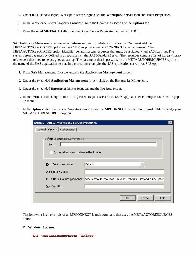
4. Under the expanded logical workspace server, right-click the Workspace Server icon and select Properties.

5. In the Workspace Server Properties window, go to the Commands section of the Options tab.

6. Enter the word METAAUTOINIT in the Object Server Parameter box and click OK.

SAS Enterprise Miner needs resources to perform automatic metadata initialization. You must add the METAAUTORESOURCES option to the SAS Enterprise Miner MPCONNECT launch command. The METAAUTORESOURCES option identifies general system resources that must be assigned when SAS starts up. The system resources must be defined in a repository on the SAS Metadata Server. The resources contain a list of librefs (library references) that need to be assigned at startup. The parameter that is passed with the METAAUTORESOURCES option is the name of the SAS application server. In the previous example, the SAS application server was SASApp.

1. From SAS Management Console, expand the Application Management folder.

2. Under the expanded Application Management folder, click on the Enterprise Miner icon.

3. Under the expanded Enterprise Miner icon, expand the Projects folder.

4. In the Projects folder, right-click the logical workspace server icon (SASApp), and select Properties from the pop-up menu.

5. In the Options tab of the Server Properties window, use the MPCONNECT launch command field to specify your METAAUTORESOURCES option.

The following is an example of an MPCONNECT launch command that uses the METAAUTORESOURCES option:

On Windows Systems:

SAS -metaautoresources "SASApp"

-config "c:\sas\eminer\lev1\sasapp\sasv9.cfg"

On UNIX Systems:

/installdir/EMiner/Lev1/SASApp/sas.sh -metaautoresources "SASApp"

ERROR: Data Set LIBREF.TABLENAME Does Not Exist

In SAS Enterprise Miner 6.1, nodes that follow a SAS Code node or custom node in a process flow diagram can produce an error that indicates that the data set that a node attempted to reference does not exist. You might get this error, even when you are able to successfully create the data source, and can explore the data set in your session. In SAS Enterprise Miner 6.1, each node in a process flow diagram spawns a new SAS session. The currently executing node does not have access to libraries that were allocated via the SAS Program Editor or a predecessor SAS Code node. In order for SAS libraries to be available to all tools and nodes in SAS Enterprise Miner 6.1, the LIBNAME statements must be specified in a location that is executed for each spawned session, such as in the project start code, the server initialization code, or SAS Management Console.


Ext Demo Node

● Overview of the Ext Demo Node● Ext Demo Node Properties● Ext Demo Node Results

Overview of the Ext Demo Node

The Ext Demo node is on the Utility tab of the Enterprise Miner toolbar. The Ext Demo node is designed to illustrate the various property types that can be implemented in Enterprise Miner extension nodes. The properties of an Enterprise Miner node enable users to pass arguments to the node's underlying SAS program. By choosing an appropriate property type, an extension node developer can control how information about the node's arguments are presented to the user and place restrictions on the values of the arguments. The Ext Demo node's results also provide examples of the various types of graphs that can be generated by an extension node using the %EM_REPORT macro.

Ext Demo Node Properties

● Ext Demo Node General Properties● Ext Demo Node Train Properties● Ext Demo Node Status Properties

Ext Demo Node General Properties

The following general properties are associated with the Ext Demo node and are

common to all Enterprise Miner nodes:

● Node ID — the ID of the node.● Imported Data — The Imported Data property provides access to the Imported

Data-Ext Demo window. The Imported Data-Ext Demo window contains a list of the ports that provide data sources to the Ext Demo node. Select the button to the right of the Imported Data property to open a table of the imported data. If data exists for an imported data source, you can select the row in the imported data table and click one of the following buttons:

�❍ Browse to open a window where you can browse the data set.�❍ Explore to open the Explore window, where you can sample and plot the

data.�❍ Properties to open the Properties window for the data source. The

Properties window contains a Table tab and a Variables tab. The tabs contain summary information (metadata) about the table and variables.

● Exported Data — The Exported Data property provides access to the Exported

Data — Ext Demo window. The Exported Data — Ext Demo window contains a list of the output data ports that the Ext Demo node creates data for when it runs. Select the button to the right of the Exported Data property to open a table that lists the exported data sets.

If data exists for an exported data set, you can select the row in the table and click one of the following buttons:

�❍ Browse to open a window where you can browse the data set.�❍ Explore to open the Explore window, where you can sample and plot the

data.�❍ Properties to open the Properties window for the data set. The Properties

window contains a Table tab and a Variables tab. The tabs contain summary information (metadata) about the table and variables.

● Variables — Use the Variables table to specify the status for individual variables that are imported into the Ext Demo Node. Select the button to open a window containing the variables table. You can set the variable status to either Use or Don't Use in the table, view the columns metadata, or open an Explore window to view a variable's sampling information, observation values, or a plot of variable distribution.

Ext Demo Node Train Properties

The Ext Demo Node has the following Train properties:

● Cell Editors �❍ Boolean — an example of a Boolean Property element that enables the

user to assign a value of Y or N to the property.�❍ String — an example of a String Property element that enables the user

to assign a character string to the property by typing the string into a text box.

�❍ Choice List — an example of a String Property element that enables the user to assign a character string to the property by selecting a string from a predetermined choice list. The choice list is implemented using a ChoiceList control.

�❍ Integer — an example of an int Property element that enables the user to assign an integer value to the property by typing the integer value into a text box. If a user types in a non-integer value, the property value is set to missing.

�❍ Integer with Range Control — an example of an int Property element that enables the user to assign a restricted integer value to the property by typing the integer value into a text box. The range is determined by the min and max attributes of the Property element. If a user types in a value that is not an integer or falls outside of the permitted range, the property value reverts back to the property's last valid value.

�❍ Double — an example of a double Property element that enables the user to assign an unrestricted real number to the property by typing a real number value into a text box. If a user types in a non-numeric value, the property's value is set to missing.

�❍ Double with Range Control — an example of a double Property element that enables the user to assign a restricted real number value to the property by typing a real number value into a text box. The range is determined by the min and max attributes of the Property element. If a user types in a value that is not a real number or falls outside of the permitted range, the property value reverts to the property's last valid value.

● Table Editors �❍ Table Editor Control Example — an example of a String Property with

a Table Editor Control. This configuration enables the user to edit or display character or numeric columns.

�❍ Table Editor with Choices — an example of a String Property with a Table Editor Control and a ChoiceList Control. This configuration enables you to restrict the values of character columns to a predetermined list of values.

�❍ Table Editor with Dynamic Choices — an example of a String Property with a Table Editor Control and a DynamicChoiceList Control. This configuration enables you to restrict the values of character columns to values that are dynamically generated by the server.

�❍ Table Editor with Restricted Choices — an example of a String Property with a Table Editor Control and a DynamicChoiceList Control. This configuration enables you to restrict the values of character columns to values that are dynamically generated by the server. In this configuration, the Table Editor Control has an attribute that enables the choice lists to differ, depending on the value of another variable.

�❍ Ordering Editor — an example of a String Property with a Table Editor Control. In this example, the Table Editor Control has an additional isOrderingEditor attribute that distinguishes it from the basic Table Editor Control. This configuration enables the user to change the order of the rows for a table.

�❍ Variables — an example of a String Property element with a Dialog Control. This Property element configuration provides access to the variables exported by a predecessor Data Source node. It is common to all SAS distributed nodes.

�❍ SASTABLE Control — an example of a String Property element with a SASTABLE Control. When the user clicks on the icon, a Select a SAS Table window is displayed and the user is permitted to select a SAS data set from the SAS libraries that are accessible by Enterprise Miner.

�❍ Text Editor — an example of a String Property with a Dialog Control. A Property with this Control configuration enables the user to enter and modify text that is stored in an external file.

�❍ Model Selector — an example of a Model Selector Control that enables the user to select a registered model. When a model is selected using this type of Control, the score code, score input variables, score output variables, target variables, training table, and fit statistics that are associated with the model are saved in the diagram folder and are associated with the node.

● Interaction Editor �❍ Two-Factor — an example of a String Property with a Dialog Control.

A Property with this Control configuration allows the user to specify a two-factor interaction. An interaction editor Control has two attributes

that determine the maximum number of effects that are allowed and whether or not main effects are allowed. This example has the maximum number of effects set to 2 and main effects are not allowed.

�❍ Terms — an example of a String Property with a Dialog Control. A Property with this Control configuration allows the user to specify main effects and up to six factor interactions. An interaction editor Control has two attributes that determine the maximum number of effects that are allowed and whether or not main effects are allowed. This example has the maximum number of effects set to 6 and main effects are allowed.

Ext Demo Node Status Properties

The following status properties are associated with the Ext Demo node and are common to all Enterprise Miner nodes:

● Create Time — displays the time that the node was created.● Run ID — displays the identifier of the run of the node. A new identifier is

created every time the node is run.● Last Error — the error message from the last run.● Last Status — the last reported status of the node.● Last Run Time — the time at which the node was last run.● Run Duration — the length of time required to complete the last node run.● Grid Host — the grid host that was used for computation.● User-Added Node — specifies whether the node was created by a user as a SAS

Enterprise Miner Extension node.

Ext Demo Node Results

You can open the Results window of the Ext Demo node by right-clicking the node and selecting Results from the pop-up menu. For more information about the Results window, see the section on the Results Window in the Enterprise Miner Help.

Select View from the main menu to view the following results in the Results Package:

● Properties �❍ Settings — displays a window with a read-only table of the configuration

information in the Ext Demo Node Properties Panel. The information was captured when the node was last run.

�❍ Run Status — indicates the status of the Ext Demo node run. The Run Start Time, Run Duration, and information about whether the run completed successfully are displayed in this window.

�❍ Variables — a read-only table of variable meta information about the data set submitted to the Ext Demo node. The table includes columns to see the variable name, the variable role, the variable level, and the model used.

�❍ Train Code — the code that Enterprise Miner used to train the node. �❍ Notes — allows users to read or create notes of interest.

● SAS Results �❍ Log — the SAS log of the Ext Demo node run.�❍ Output — the SAS output of the Ext Demo node run. �❍ Flow Code — the SAS code used to produce the output that the Ext Demo

node passes on to the next node in the process flow diagram. ● Scoring

�❍ SAS Code — the Ext Demo node does not generate SAS Code. The SAS Code menu item is dimmed and unavailable in the Ext Demo Results window.

�❍ PMML Code — the Ext Demo node does not generate PMML code. The PMML Code menu item is dimmed and unavailable in the Ext Demo Results window menu.

The Ext Demo node results also include a collection of charts that can be generated using the %EM_REPORT macro. These include the following:

● Bar Chart �❍ Simple �❍ Combo Choices

● Histogram �❍ Simple �❍ Combo Choices

● Line Plot �❍ Simple �❍ Overlay �❍ Reference Lines �❍ Combo Choices �❍ Overlay Combo Choices

�❍ Two Y Axes �❍ Two Y Axes Combo Choices �❍ Line Band �❍ Group

● Scatter Plot �❍ Simple �❍ Overlay �❍ Combo Choices �❍ Overlay Combo Choices �❍ Group

● Pie �❍ Simple

● Lattice �❍ Simple Bar �❍ Bar Combo Choices �❍ Simple Histogram �❍ Histogram Combo Choices �❍ Simple Line Plot �❍ Line Plot Overlay �❍ Line Plot Reference Lines �❍ Line Plot Combo Choices �❍ Pie

● Box Plot �❍ Grouped

● 3-D Graphs �❍ Scatter Plot �❍ Bar �❍ Surface

● Data Specific �❍ Dendrogram �❍ Constellation: Link and Node Data �❍ Constellation: Link Data

If you place an options mprint; statement in your project start code, the calls to %em_report are recorded in the Results log. You can also view the ExtDemo node's source code. It is stored in Sashelp.Emutil.Extdemo.source.


SAS Enterprise Miner 6.1 Extension Nodes: Developer's Guide

Documents

Transcript of SAS Enterprise Miner 6.1 Extension Nodes: Developer's Guide