Sales Forecasting for Manufacturers -...

Sales Forecasting for ManufacturersPrepared by:

Chris Holling, Managing Executive DirectorBusiness Planning Solutions, Advisory Services Division

Joyce BrinnerSenior Principal, Business Planning Solutions

Webcast5 June 2007

Business-to-Business Sales Forecasting

Prepared by:Chris Holling, Managing Executive Director

Business Planning Solutions, Advisory Services Division

5 June 2007

Copyright © 2007 Global Insight, Inc. 3

Understand Your Business Drivers, Forecast Your Sales…

…& Manage Business Cycle Risk.ROI from Forecasting:

Increasing the accuracy of your forecasting or

advance planning process can generate

significant returns


…& Manage Business Cycle Risk.


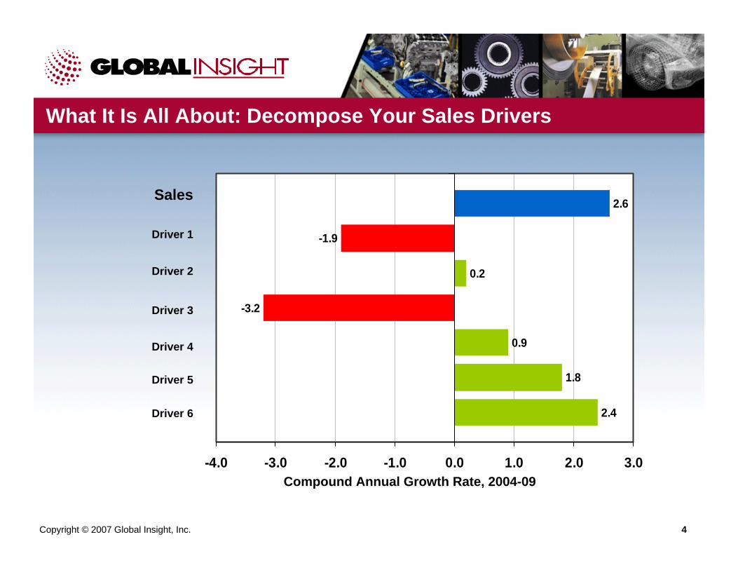
2.4

1.8

0.9

-3.2

0.2

-1.9

2.6

-4.0 -3.0 -2.0 -1.0 0.0 1.0 2.0 3.0

Driver 3

Driver 2

Driver 1

Driver 4

Driver 5

Driver 6

Compound Annual Growth Rate, 2004-09

Sales

What It Is All About: Decompose Your Sales Drivers


From the Strategic to the Tactical (and Back)…

Insight on your business drivers–for telling the story to Wall Street


Keys to Success in Sales Forecasting

Be clear and explicit about how things work. Focus on causality, not correlation.Common sense always trumps econometrics and “sophisticated” statistical techniques.Process is king: developing internal alignment is more important than the model itself.


What Works Best

• The model is anchored by business unit management knowledge of the distribution of their sales across key end-markets—B2B and consumer.

• The system clearly decomposes historical, current, and future sales into:

Market volume growth,Price changes, and Share gains/losses due to new products or competitive initiatives.

• The model is simple and embodies common sense causal relationships.


What Does Not Work

• A forecasting process tied to “black-box”regressions, correlations, data mining, or pressure curves to “explain” the past or forecast the future.

• Models linked to overly “macro” concepts like total GDP, total industrial production and not to the specific, causal drivers that affect the company.


Keep Grounded in Common Sense

• THINK about your common sense expectations about how things work — your “a priori” assumptions.

• LOOK at many time series charts of the dependent and possible independent variables. Develop a basic “story”about what is really going on.

• LEARN from how the equations or models from other projects were structured.

• DESIGN your initial model specification on paper first. Think about ways to normalize data to get at fundamental relationships and control for serial correlation.

• THINK BASIC – focus on the core causal relationships between drivers and sales.


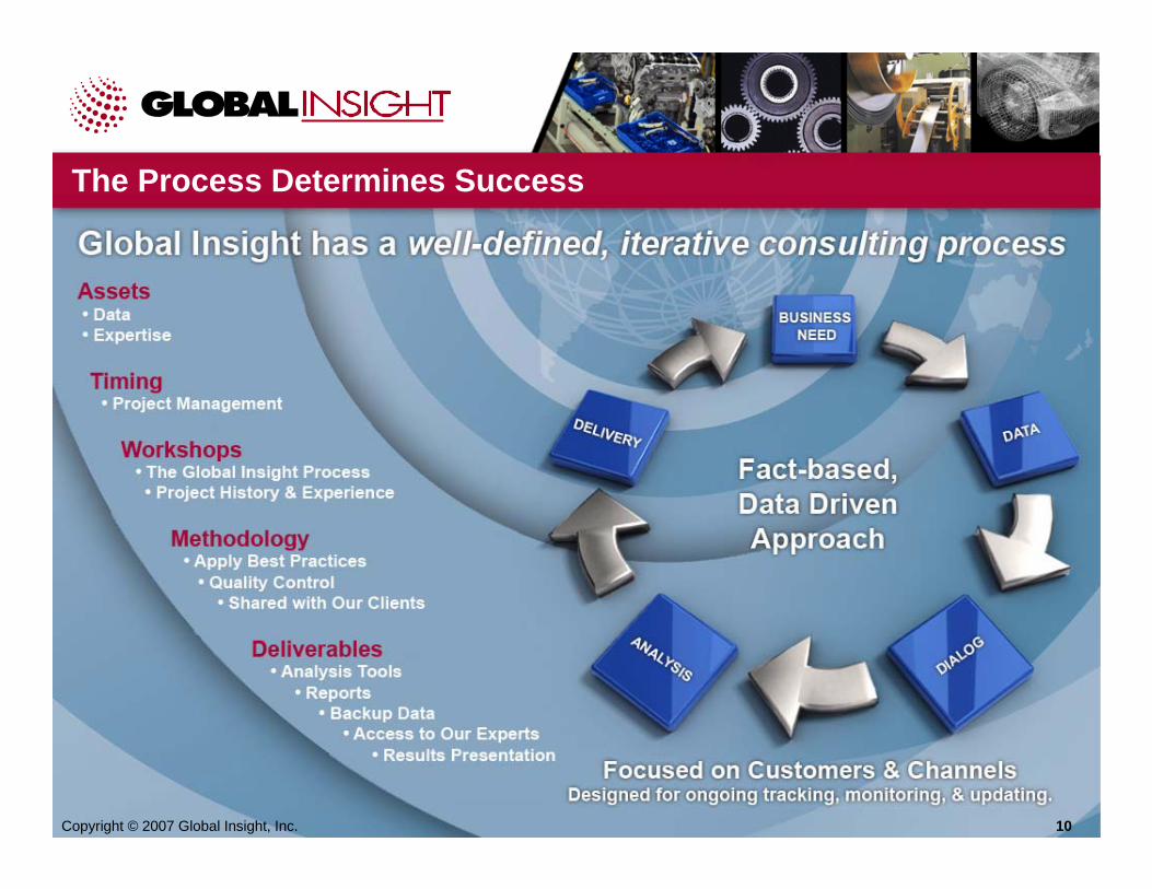
The Process Determines Success



Separate Drivers of New Demand vs. Replacement Demand

• New Demand: OEM production, construction, or retooling of customer manufacturing operations.

• Replacement Demand: product life span, technological change, “wear and tear” parts and products.

New demand tends to be more cyclical than replacement demand.


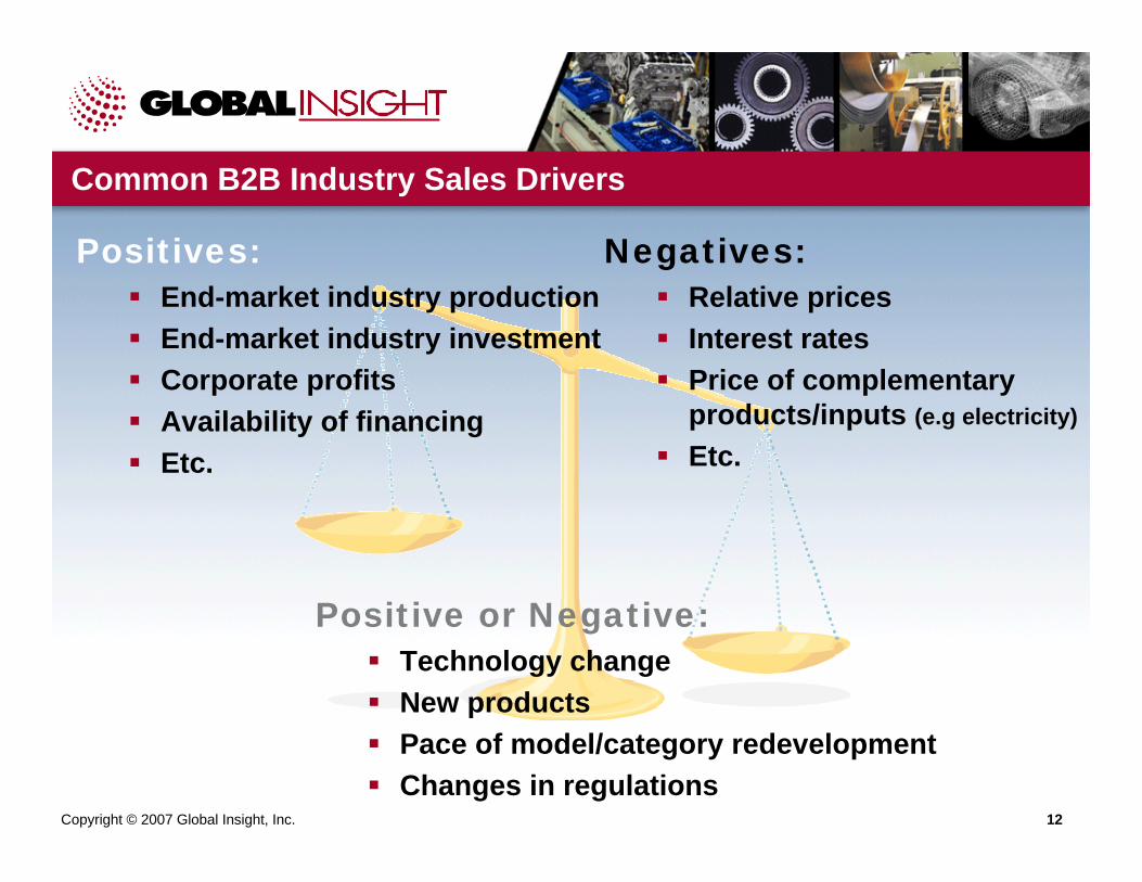
Common B2B Industry Sales Drivers

Positives:End-market industry productionEnd-market industry investmentCorporate profitsAvailability of financingEtc.

Negatives:Relative pricesInterest ratesPrice of complementary products/inputs (e.g electricity)

Etc.

Positive or Negative:Technology changeNew productsPace of model/category redevelopmentChanges in regulations


Common Company Market Share Drivers

• Product positioning/ targeting that is different from the industry average

• Price• Financing activity• Promotion activity• Product rationalization• Sales force/distribution

channel management• Acquisitions/divestitures


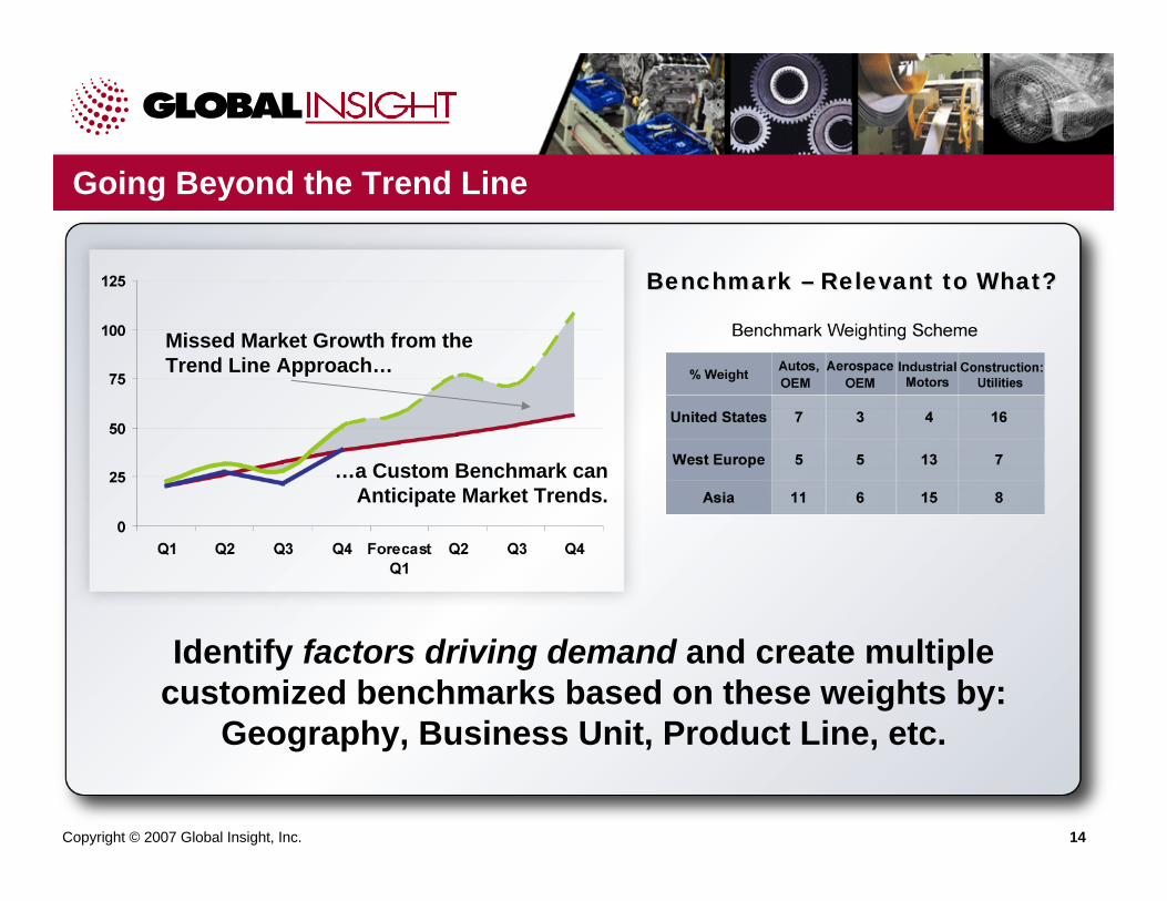
Going Beyond the Trend Line

Identify factors driving demand and create multiple customized benchmarks based on these weights by:

Geography, Business Unit, Product Line, etc.

…a Custom Benchmark can Anticipate Market Trends.

Missed Market Growth from the Trend Line Approach…

Benchmark – Relevant to What?Benchmark – Relevant to What?


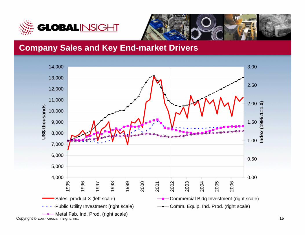
Company Sales and Key End-market Drivers

4,000

5,000

6,000

7,000

8,000

9,000

10,000

11,000

12,000

13,000

14,00019

95

1996

1997

1998

1999

2000

2001

2002

2003

2004

2005

2006

US$

thou

sand

s

0.00

0.50

1.00

1.50

2.00

2.50

3.00

Inde

x (1

995:

1=1.

0)

Sales: product X (left scale) Commercial Bldg Investment (right scale)Public Utility Investment (right scale) Comm. Equip. Ind. Prod. (right scale)Metal Fab. Ind. Prod. (right scale)


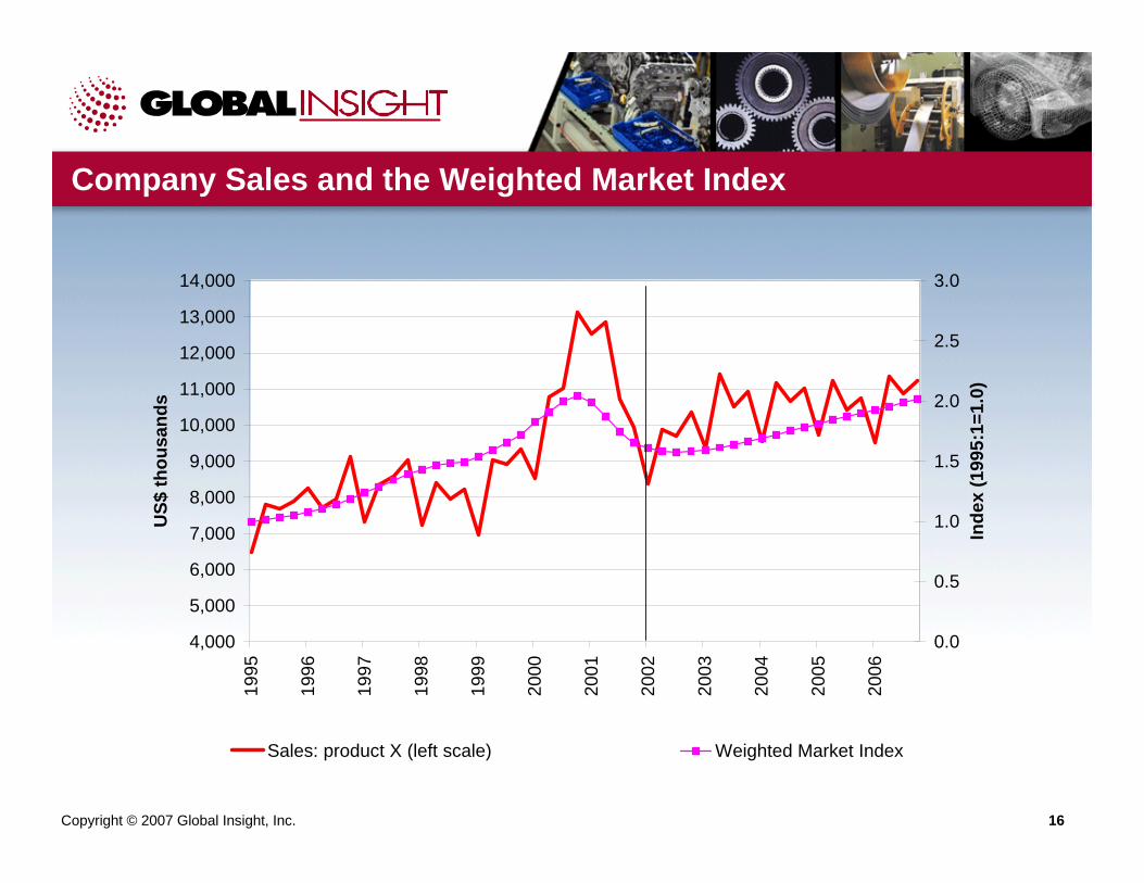
Company Sales and the Weighted Market Index

4,000

5,000

6,000

7,000

8,000

9,000

10,000

11,000

12,000

13,000

14,00019

95

1996

1997

1998

1999

2000

2001

2002

2003

2004

2005

2006

US$

thou

sand

s

0.0

0.5

1.0

1.5

2.0

2.5

3.0

Inde

x (1

995:

1=1.

0)

Sales: product X (left scale) Weighted Market Index


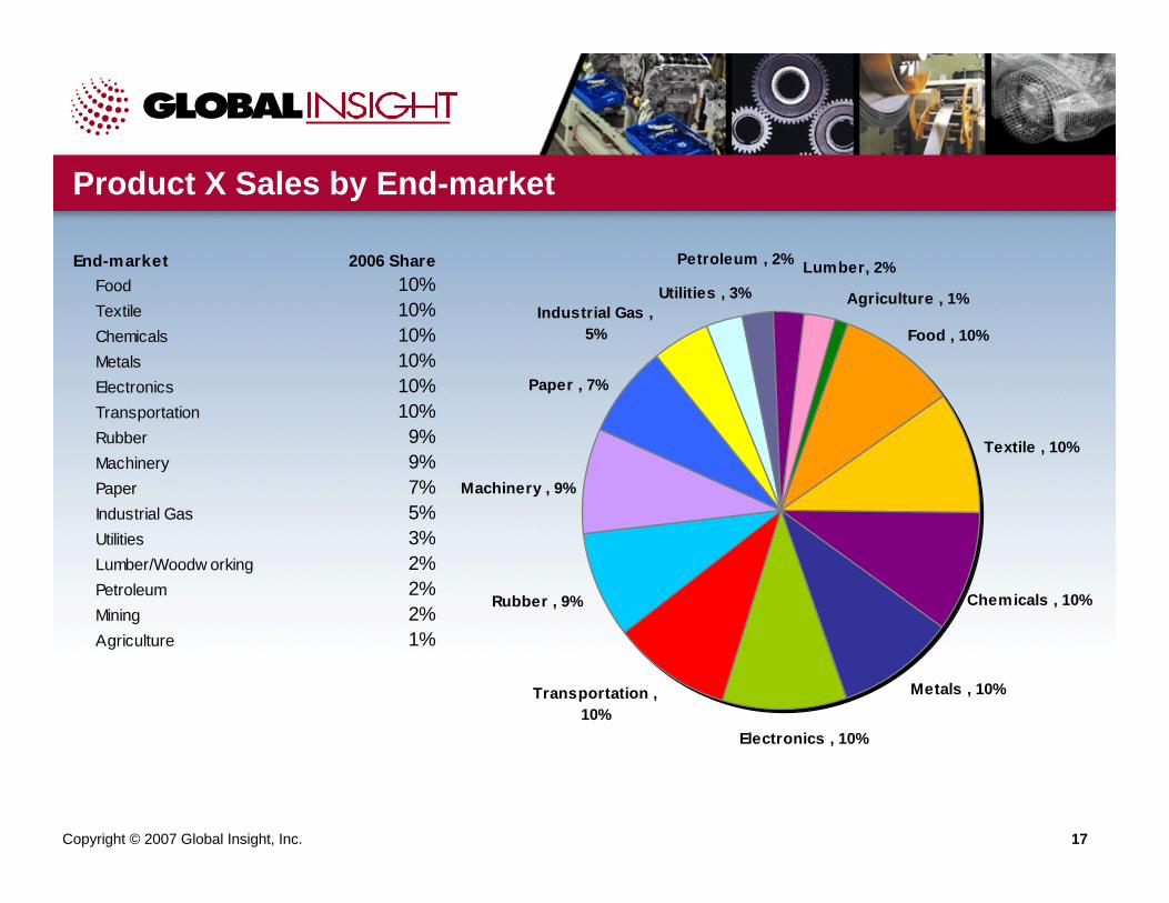
Product X Sales by End-market

Metals , 10%

Textile , 10%

Chemicals , 10%

Petroleum , 2%

Paper , 7%

Machinery , 9%

Utilities , 3% Industrial Gas ,

5%

Lumber, 2%

Agriculture , 1%

Electronics , 10%

Transportation , 10%

Rubber , 9%

Food , 10%

End-market 2006 Share Food 10% Textile 10% Chemicals 10% Metals 10% Electronics 10% Transportation 10% Rubber 9% Machinery 9% Paper 7% Industrial Gas 5% Utilities 3% Lumber/Woodw orking 2% Petroleum 2% Mining 2% Agriculture 1%


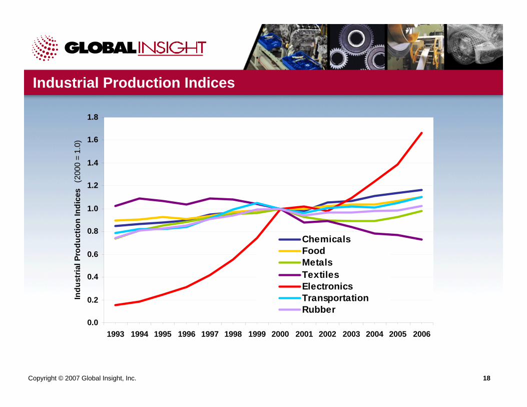
Industrial Production Indices

0.0

0.2

0.4

0.6

0.8

1.0

1.2

1.4

1.6

1.8

1993 1994 1995 1996 1997 1998 1999 2000 2001 2002 2003 2004 2005 2006

Indu

stria

l Pro

duct

ion

Indi

ces

(200

0 =

1.0)

ChemicalsFoodMetalsTextilesElectronicsTransportationRubber


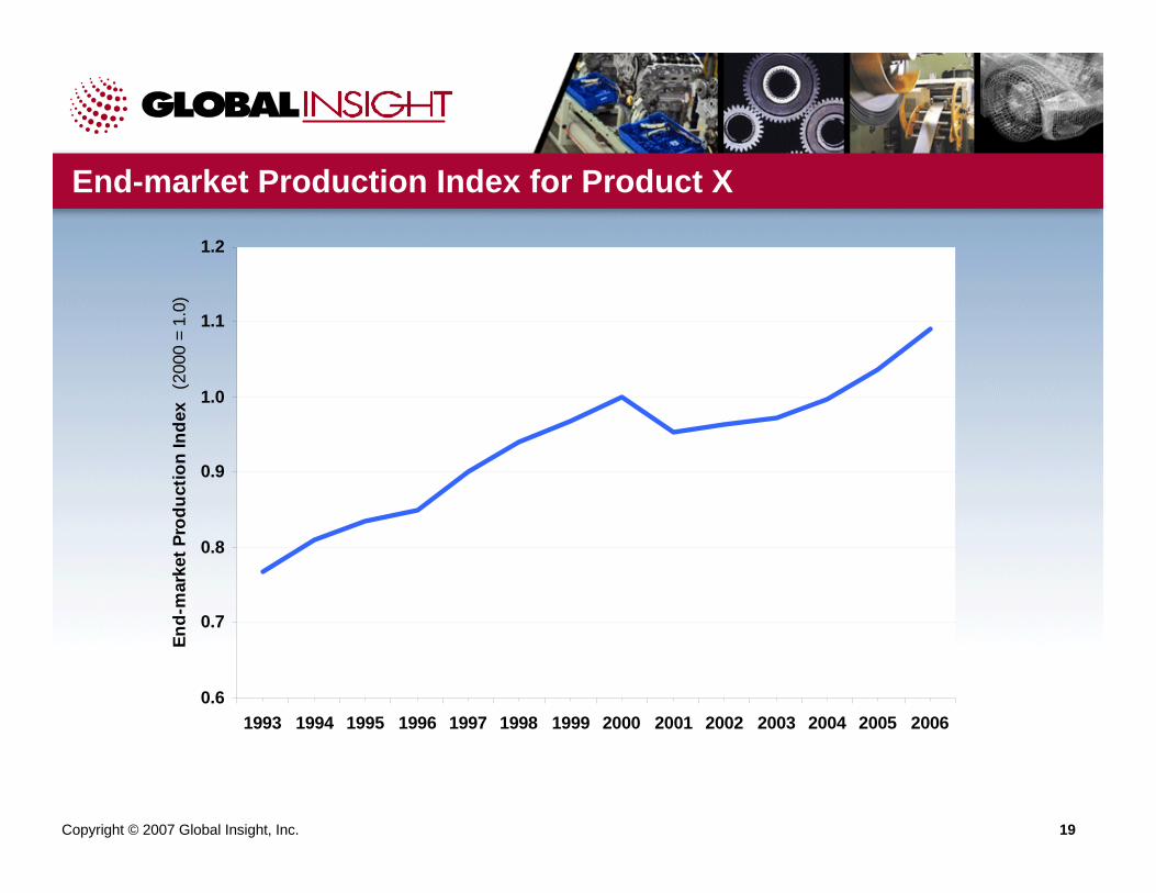
End-market Production Index for Product X

0.6

0.7

0.8

0.9

1.0

1.1

1.2

1993 1994 1995 1996 1997 1998 1999 2000 2001 2002 2003 2004 2005 2006

End-

mar

ket P

rodu

ctio

n In

dex

(200

0 =

1.0)


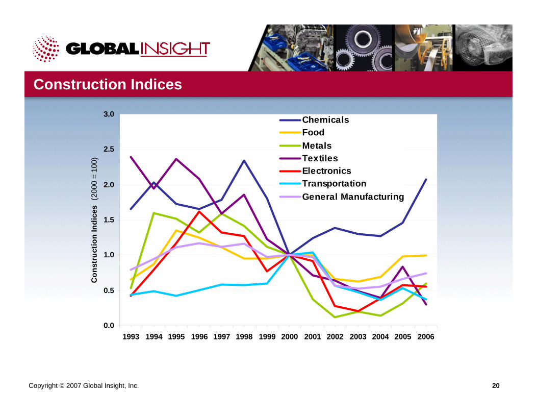
Construction Indices

0.0

0.5

1.0

1.5

2.0

2.5

3.0

1993 1994 1995 1996 1997 1998 1999 2000 2001 2002 2003 2004 2005 2006

Con

stru

ctio

n In

dice

s (2

000

= 10

0)

ChemicalsFoodMetalsTextilesElectronicsTransportationGeneral Manufacturing


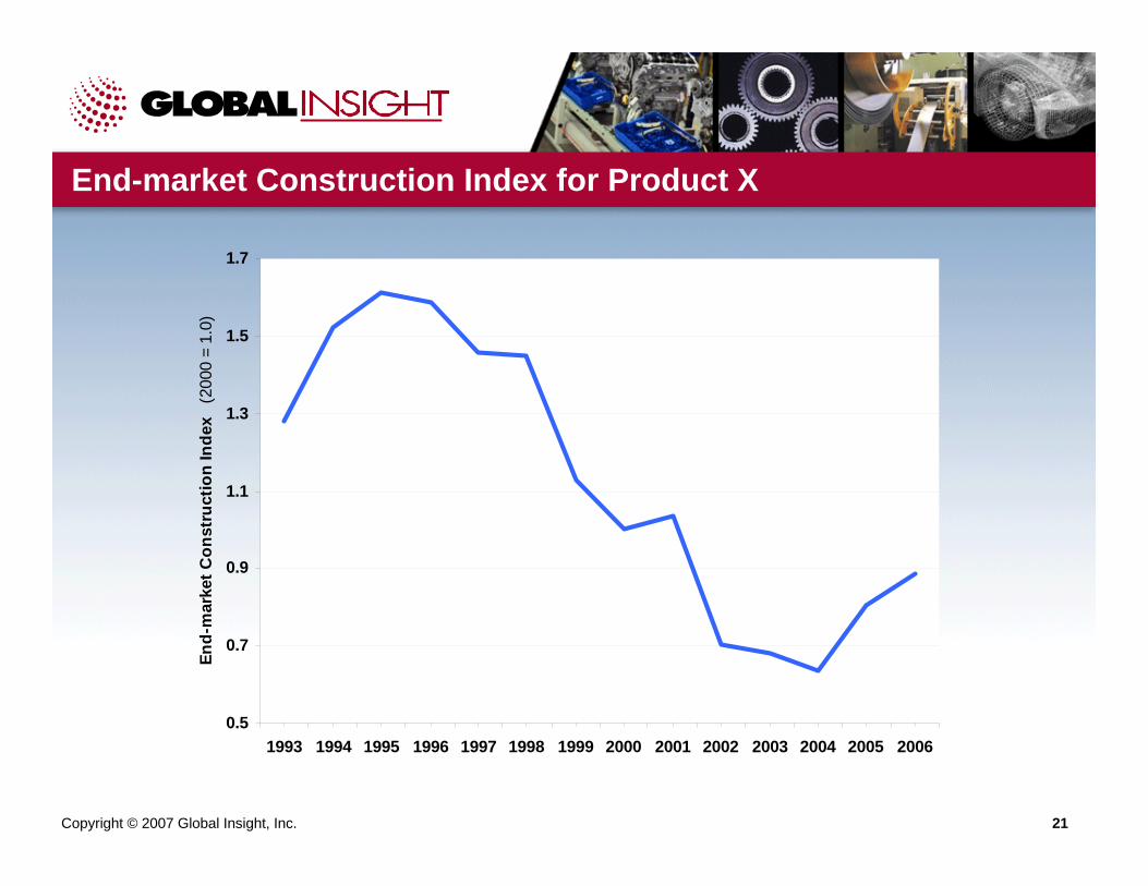
End-market Construction Index for Product X

0.5

0.7

0.9

1.1

1.3

1.5

1.7

1993 1994 1995 1996 1997 1998 1999 2000 2001 2002 2003 2004 2005 2006

End-

mar

ket C

onst

ruct

ion

Inde

x (2

000

= 1.

0)


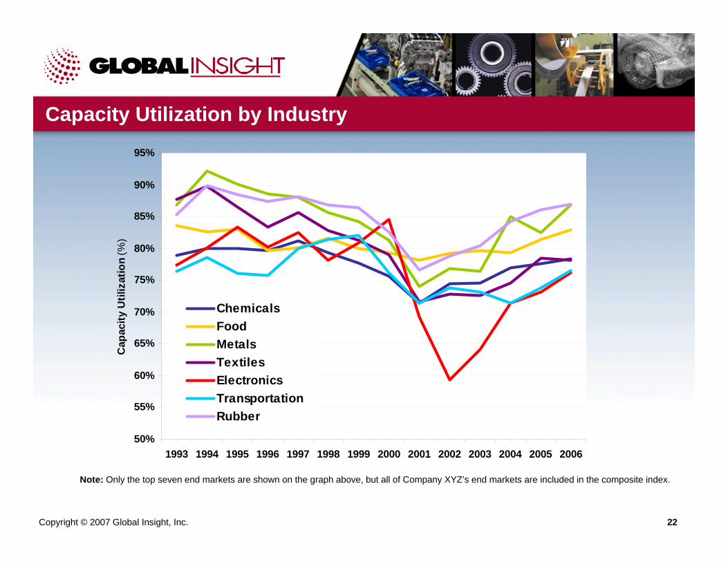
Capacity Utilization by Industry

50%

55%

60%

65%

70%

75%

80%

85%

90%

95%

1993 1994 1995 1996 1997 1998 1999 2000 2001 2002 2003 2004 2005 2006

Cap

acity

Util

izat

ion

(%)

ChemicalsFoodMetalsTextilesElectronicsTransportationRubber

Note: Only the top seven end markets are shown on the graph above, but all of Company XYZ’s end markets are included in the composite index.


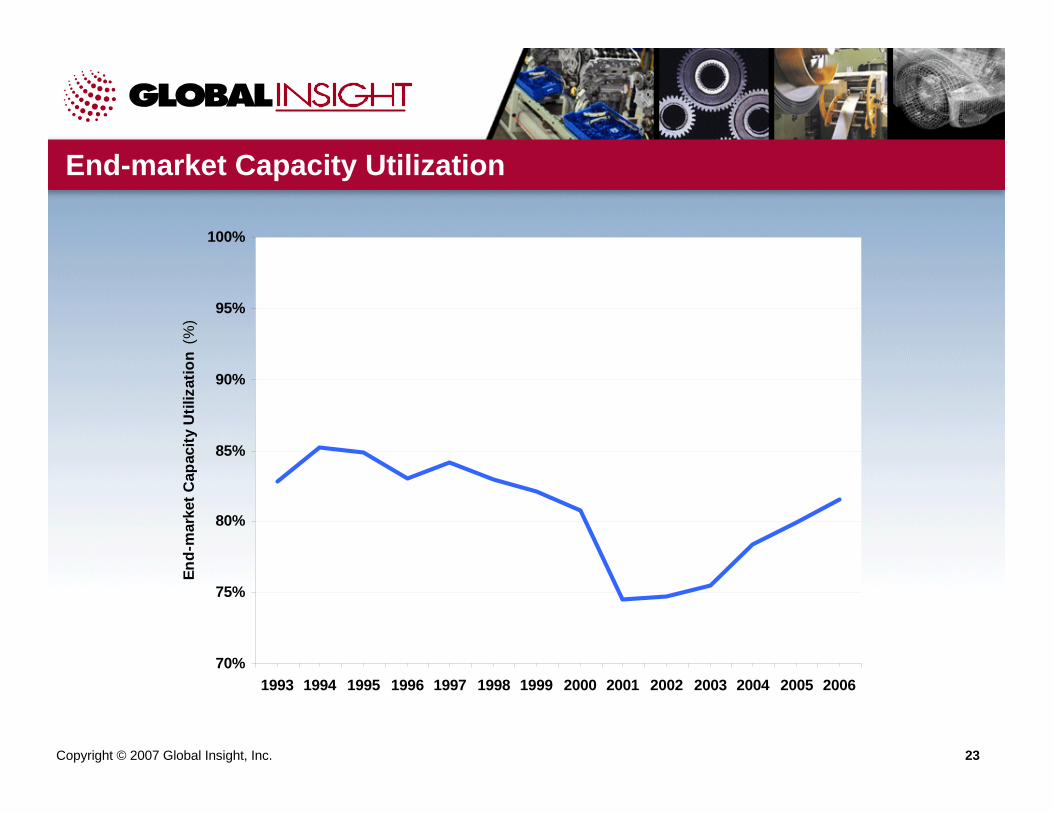
End-market Capacity Utilization

70%

75%

80%

85%

90%

95%

100%

1993 1994 1995 1996 1997 1998 1999 2000 2001 2002 2003 2004 2005 2006

End-

mar

ket C

apac

ity U

tiliz

atio

n (%

)


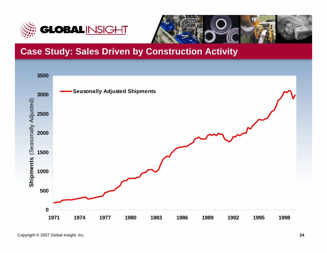
Case Study: Sales Driven by Construction Activity

0

500

1000

1500

2000

2500

3000

3500

1971 1974 1977 1980 1983 1986 1989 1992 1995 1998

Ship

men

ts (

Seas

onal

ly A

djus

ted)

Seasonally Adjusted Shipments


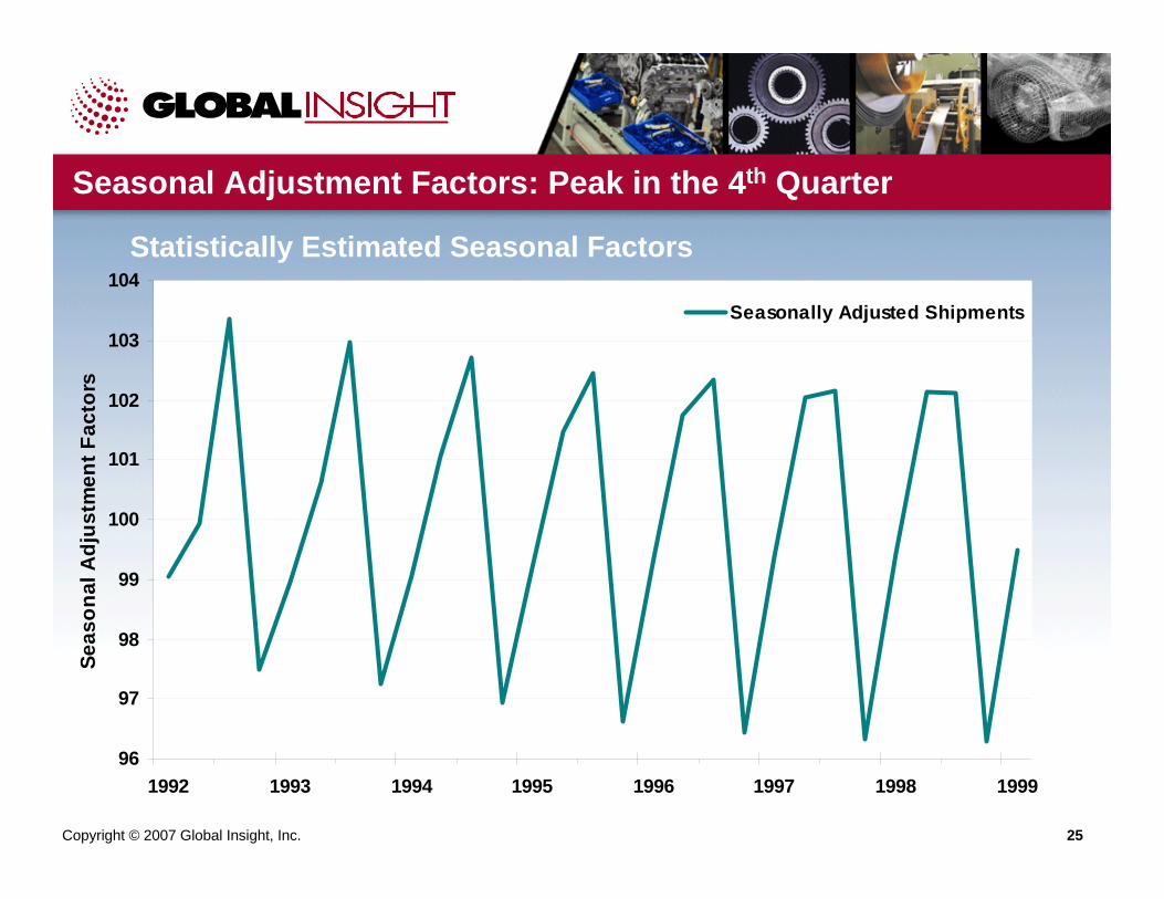
96

97

98

99

100

101

102

103

104

1992 1993 1994 1995 1996 1997 1998 1999

Seas

onal

Adj

ustm

ent F

acto

rs

Seasonally Adjusted Shipments

Seasonal Adjustment Factors: Peak in the 4th Quarter

Statistically Estimated Seasonal Factors


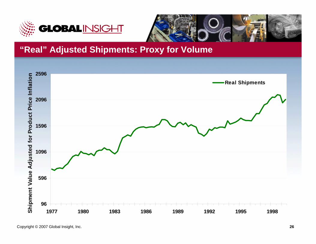
“Real” Adjusted Shipments: Proxy for Volume

96

596

1096

1596

2096

2596

1977 1980 1983 1986 1989 1992 1995 1998Ship

men

t Val

ue A

djus

ted

for P

rodu

ct P

rice

Infla

tion

Real Shipments


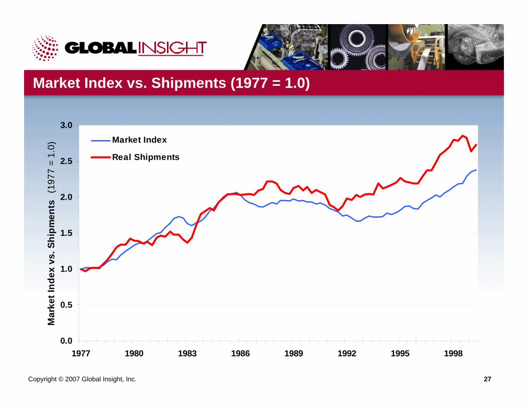
Market Index vs. Shipments (1977 = 1.0)

0.0

0.5

1.0

1.5

2.0

2.5

3.0

1977 1980 1983 1986 1989 1992 1995 1998

Mar

ket I

ndex

vs.

Shi

pmen

ts

(197

7 =

1.0)

Market Index

Real Shipments


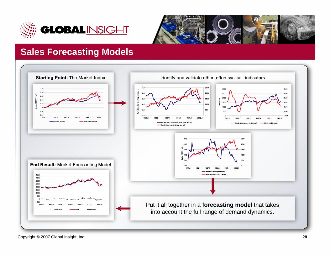
Sales Forecasting Models

Put it all together in a forecasting model that takes into account the full range of demand dynamics.


Econometric Modeling Principles – Some Technical Notes

As you begin regression analysis, consider the following:Each time you run a regression, see if the coefficients match a priori expectations and look at how it forecasts. Remember the goal is not an equation with a high R-squared, it is an equation that forecasts well.Don’t let a regression convince you that basic economic theory is wrong. A positive price elasticity or an income elasticity of 10 is not an exciting new discovery — it is evidence of a mis-specified model.Always look at a time series chart of the residuals and think about how what you see may be a clue to a missing variable.Lagged dependent variable and Autoregressive (AR) corrections may happen only at the very end of a modeling process as a last resort to fine tune — authorized by the Project Director.


Dashboard Reports

30

Implement a sales benchmarking program for each business unitFormalize your market index in the form of a corporate dashboard

Global Consumer Buying Power: Segmentation and Forecasts

Prepared by:Joyce Brinner

Senior Principal, Business Planning Solutions


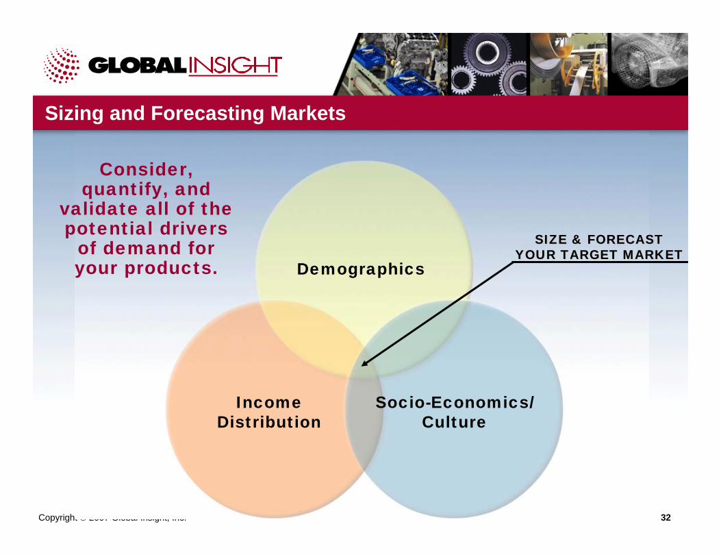
Sizing and Forecasting Markets

Income Distribution

Socio-Economics/Culture

Demographics

SIZE & FORECAST SIZE & FORECAST YOUR TARGET MARKETYOUR TARGET MARKET

Consider, quantify, and

validate all of the potential drivers

of demand for your products.


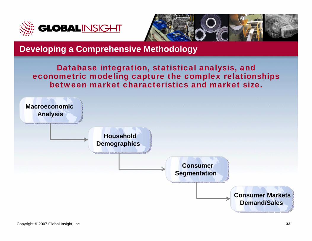
Developing a Comprehensive Methodology

Database integration, statistical analysis, and econometric modeling capture the complex relationships

between market characteristics and market size.

HouseholdDemographics

HouseholdDemographics

Macroeconomic Analysis

Macroeconomic Analysis

ConsumerSegmentation

ConsumerSegmentation

Consumer MarketsDemand/Sales

Consumer MarketsDemand/Sales


The Key to a Successful Model

• Include the appropriate concepts

• Represent the true timing of reactions

• Possess coefficients with the appropriate magnitudes

• Earn the confidence of users

To be successful, a model must:



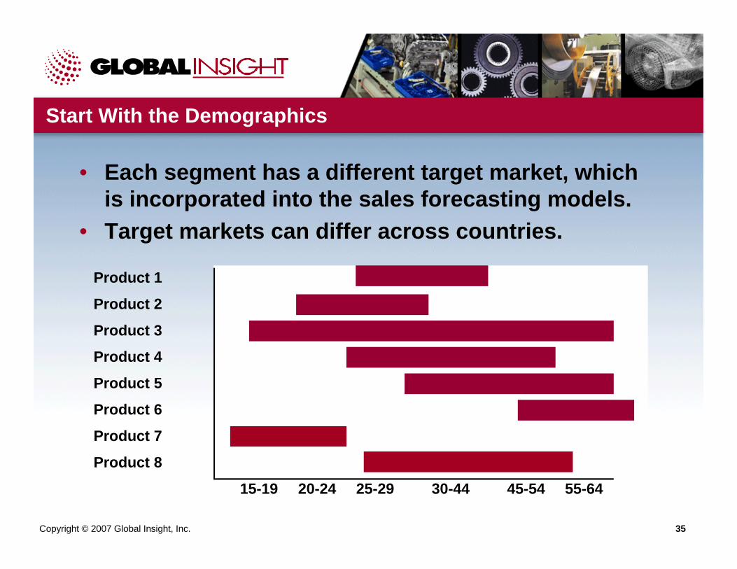
Start With the Demographics

• Each segment has a different target market, which is incorporated into the sales forecasting models.

• Target markets can differ across countries.

Product 1

Product 2

Product 3

Product 4

Product 5

Product 6

Product 7

Product 8

15-19 20-24 25-29 30-44 45-54 55-64


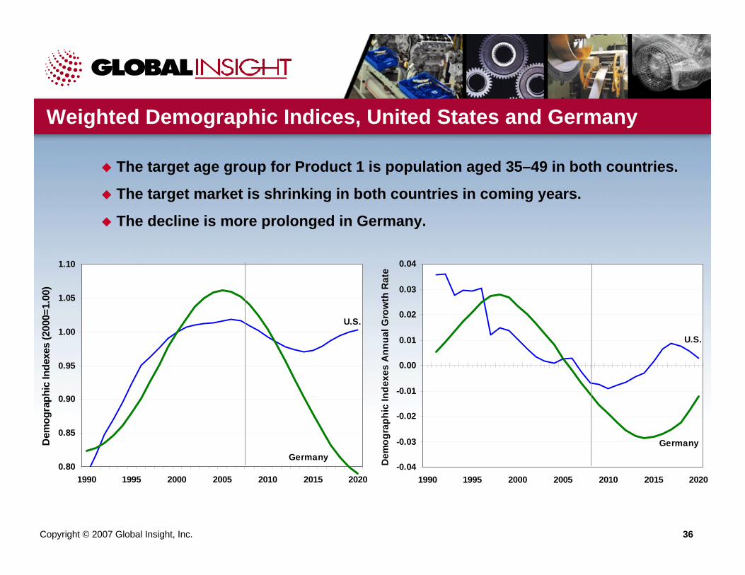
Weighted Demographic Indices, United States and Germany

The target age group for Product 1 is population aged 35–49 in both countries.

The target market is shrinking in both countries in coming years.

The decline is more prolonged in Germany.

0.80

0.85

0.90

0.95

1.00

1.05

1.10

1990 1995 2000 2005 2010 2015 2020

Dem

ogra

phic

Inde

xes

(200

0=1.

00)

U.S.

Germany-0.04

-0.03

-0.02

-0.01

0.00

0.01

0.02

0.03

0.04

1990 1995 2000 2005 2010 2015 2020

Dem

ogra

phic

Inde

xes

Ann

ual G

row

th R

ate

U.S.

Germany


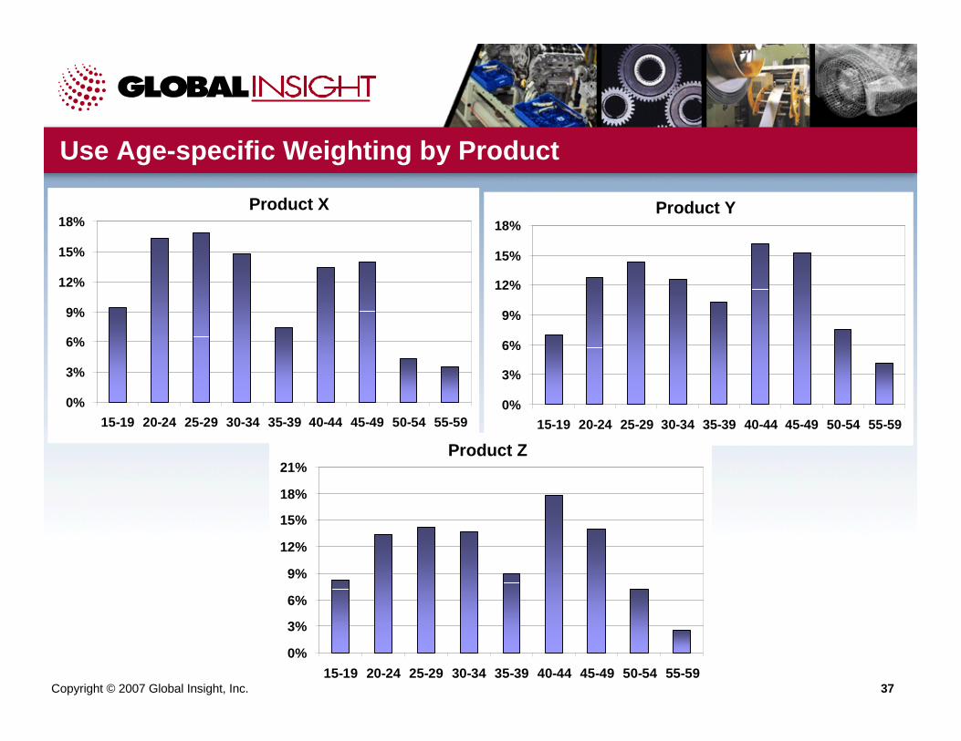
Use Age-specific Weighting by Product

Body

0%

3%

6%

9%

12%

15%

18%

15-19 20-24 25-29 30-34 35-39 40-44 45-49 50-54 55-59

Face

0%

3%

6%

9%

12%

15%

18%

15-19 20-24 25-29 30-34 35-39 40-44 45-49 50-54 55-59

Sun

0%

3%

6%

9%

12%

15%

18%

21%

15-19 20-24 25-29 30-34 35-39 40-44 45-49 50-54 55-59

Product X Product Y

Product Z


Major Appliances

0

100

200

300

400

500

600

700

800

900

All < 25 25-34 35-44 45-54 55-64 65-74 75+

Women's Apparel

0

100

200

300

400

500

600

700

800

900

All < 25 25-34 35-44 45-54 55-64 65-74 75+

Men's Apparel

0

100

200

300

400

500

600

700

800

900

All < 25 25-34 35-44 45-54 55-64 65-74 75+

Furniture

0

100

200

300

400

500

600

700

800

900

All < 25 25-34 35-44 45-54 55-64 65-74 75+

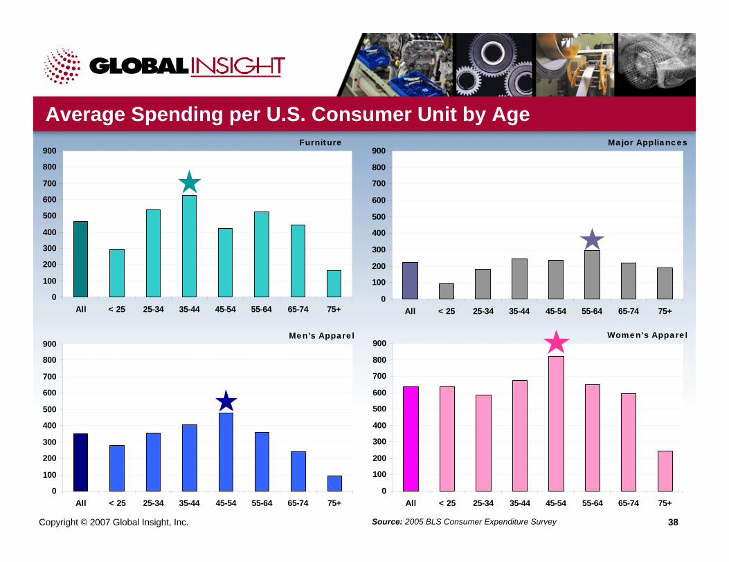
Average Spending per U.S. Consumer Unit by Age

Source: 2005 BLS Consumer Expenditure Survey


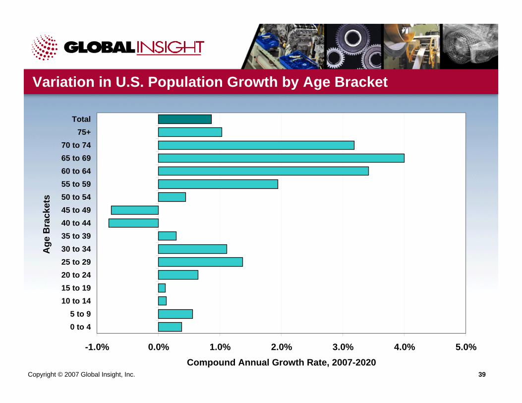
Variation in U.S. Population Growth by Age Bracket

-1.0% 0.0% 1.0% 2.0% 3.0% 4.0% 5.0%

0 to 45 to 9

10 to 1415 to 1920 to 2425 to 2930 to 3435 to 3940 to 4445 to 4950 to 5455 to 5960 to 6465 to 6970 to 74

75+Total

Age

Bra

cket

s

Compound Annual Growth Rate, 2007-2020


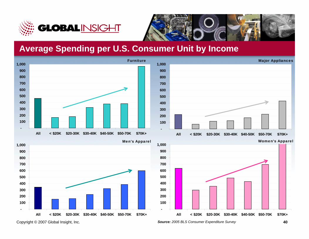
Major Appliances

-

100

200

300

400

500

600

700

800

900

1,000

All < $20K $20-30K $30-40K $40-50K $50-70K $70K+

Women's Apparel

-

100

200

300

400

500600

700

800

900

1,000

All < $20K $20-30K $30-40K $40-50K $50-70K $70K+

Men's Apparel

-

100

200300

400

500

600

700800

900

1,000

All < $20K $20-30K $30-40K $40-50K $50-70K $70K+

Furniture

-

100200

300

400

500600

700

800900

1,000

All < $20K $20-30K $30-40K $40-50K $50-70K $70K+

Average Spending per U.S. Consumer Unit by Income

Source: 2005 BLS Consumer Expenditure Survey


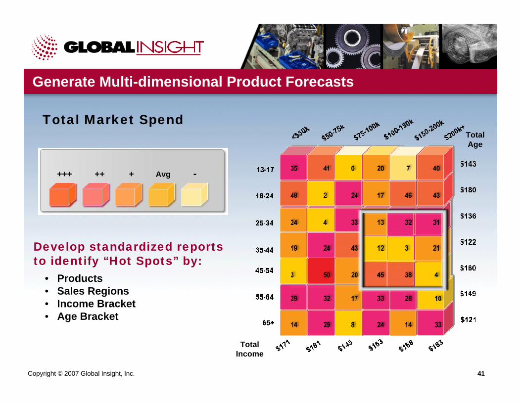
Generate Multi-dimensional Product Forecasts

Total Market Spend

TotalIncome

TotalAge

+++ ++ + Avg -

Develop standardized reports to identify “Hot Spots” by:

• Products• Sales Regions• Income Bracket• Age Bracket


Put it all together in a forecasting model that takes into account the full range of demand dynamics.

Starting Point: Trend Analysis Identify and validate economic and industry drivers

Ending Point: Forecasting Model


Consider All the Drivers


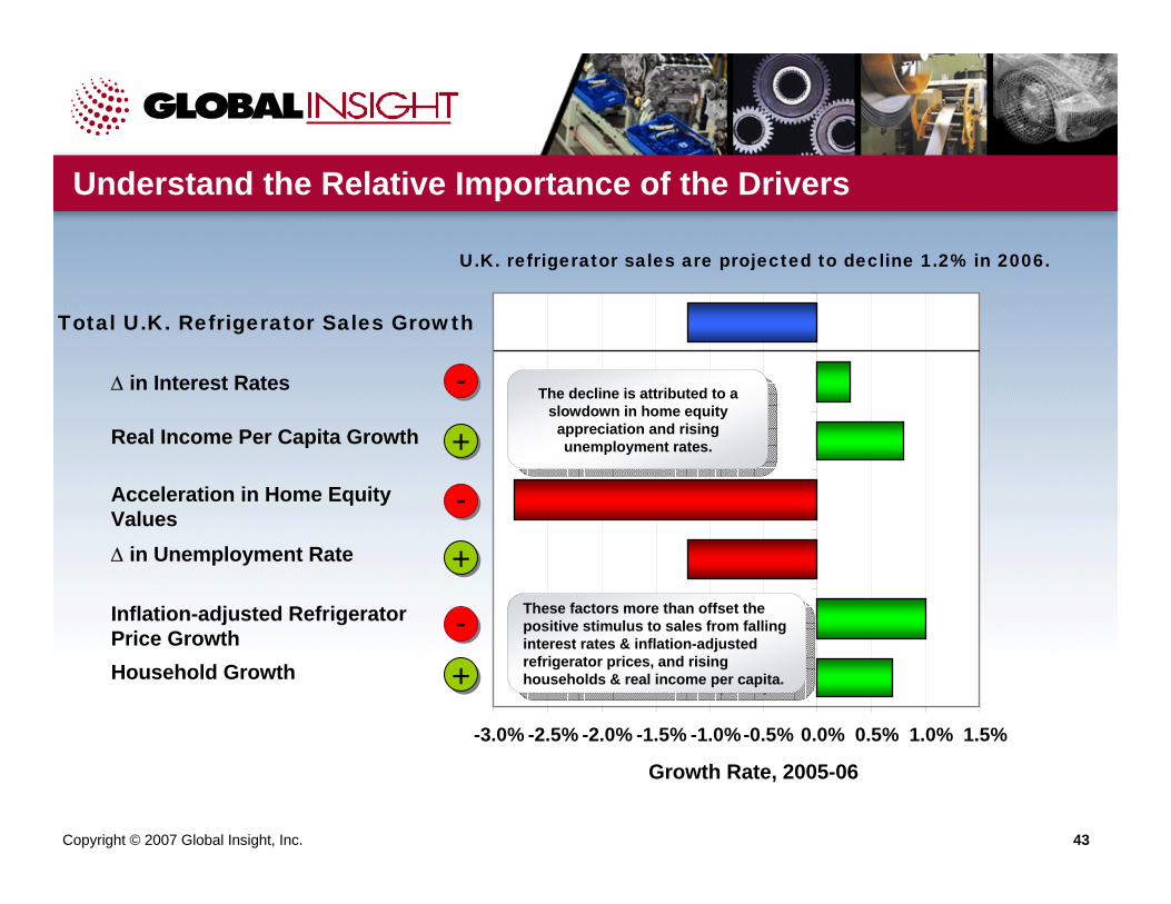
Understand the Relative Importance of the Drivers

Household Growth

Inflation-adjusted Refrigerator Price Growth

∆ in Unemployment Rate

Acceleration in Home Equity Values

Real Income Per Capita Growth

∆ in Interest Rates

Total U.K. Refrigerator Sales Growth

-3.0% -2.5% -2.0% -1.5% -1.0%-0.5% 0.0% 0.5% 1.0% 1.5%

Growth Rate, 2005-06

--

--

--

++

++

++

U.K. refrigerator sales are projected to decline 1.2% in 2006.

The decline is attributed to a slowdown in home equity

appreciation and rising unemployment rates.

The decline is attributed to a slowdown in home equity

appreciation and rising unemployment rates.

These factors more than offset the positive stimulus to sales from falling interest rates & inflation-adjusted refrigerator prices, and rising households & real income per capita.

These factors more than offset the positive stimulus to sales from falling interest rates & inflation-adjusted refrigerator prices, and rising households & real income per capita.


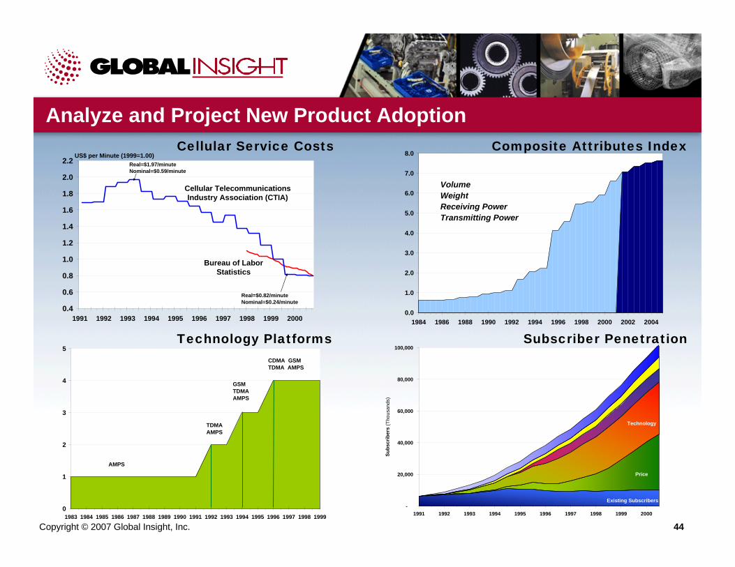
0

1

2

3

4

5

1983 1984 1985 1986 1987 1988 1989 1990 1991 1992 1993 1994 1995 1996 1997 1998 1999

AMPS

TDMAAMPS

GSMTDMAAMPS

CDMA GSMTDMA AMPS

0.4

0.6

0.8

1.0

1.2

1.4

1.6

1.8

2.0

2.2

1991 1992 1993 1994 1995 1996 1997 1998 1999 2000

Bureau of Labor Statistics

Cellular Telecommunications Industry Association (CTIA)

US$ per Minute (1999=1.00)Real=$1.97/minuteNominal=$0.59/minute

Real=$0.82/minuteNominal=$0.24/minute

0.0

1.0

2.0

3.0

4.0

5.0

6.0

7.0

8.0

1984 1986 1988 1990 1992 1994 1996 1998 2000 2002 2004

Analyze and Project New Product Adoption

Subscriber Penetration

Cellular Service Costs Composite Attributes Index

Technology Platforms

VolumeWeightReceiving PowerTransmitting Power

-

20,000

40,000

60,000

80,000

100,000

1991 1992 1993 1994 1995 1996 1997 1998 1999 2000

Subs

crib

ers

(Tho

usan

ds)

Existing Subscribers

Price

Technology


0

100

200

300

400

500

600

700

800

900

0 5000 10000 15000 20000 25000 30000 35000 40000 45000GDP per Capita (2000 US $)

Com

mun

icat

ions

Spe

nd p

er C

apita

(200

0 U

S $

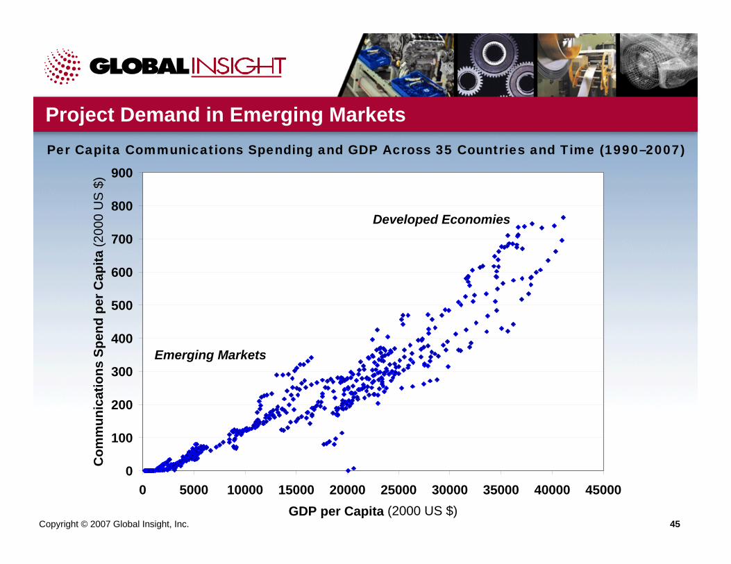
)Project Demand in Emerging MarketsPer Capita Communications Spending and GDP Across 35 Countries and Time (1990–2007)

Emerging Markets

Developed Economies


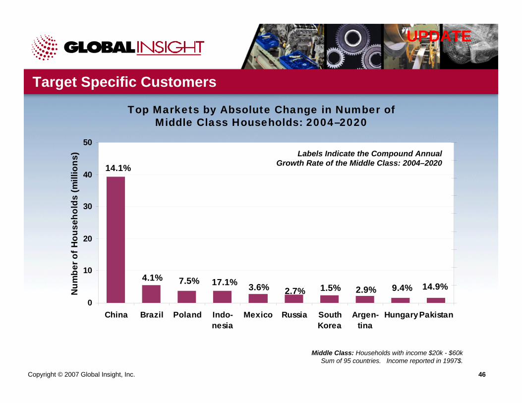
Target Specific Customers

Middle Class: Households with income $20k - $60kSum of 95 countries. Income reported in 1997$.

3.6% 2.7% 2.9% 14.9%9.4%1.5%17.1%7.5%4.1%

14.1%

0

10

20

30

40

50

China Brazil Poland Indo-nesia

Mexico Russia SouthKorea

Argen-tina

HungaryPakistan

Num

ber o

f Hou

seho

lds

(mill

ions

) Labels Indicate the Compound Annual Growth Rate of the Middle Class: 2004–2020

Top Markets by Absolute Change in Number of Middle Class Households: 2004–2020

UPDATE


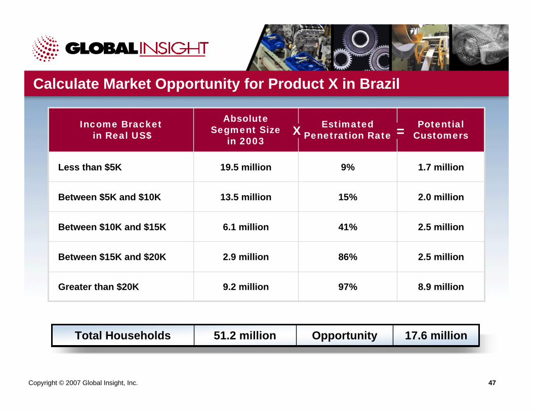
Calculate Market Opportunity for Product X in Brazil

8.9 million97%9.2 millionGreater than $20K

2.5 million86%2.9 millionBetween $15K and $20K



1.7 million9%19.5 millionLess than $5K

Potential Customers

Estimated Penetration Rate

Absolute Segment Size

in 2003

Income Bracketin Real US$ X =

17.6 millionOpportunity51.2 millionTotal Households


Data are Dumb…You Must be Smart

Structural modeling — most trustworthySearch for causation, not correlation.Be clear whether you are modeling demand or supply – only one per equation.

T-statistics are often misinterpretedTs measure precision of estimate, not whether a factor is important.Multicolinearity must be dealt with through constraints, not exclusion of good factors.



Benchmark Results Against Relevant Experience

• Counter-intuitive elasticities are usually a sign of spurious correlation, data errors, or multicolinearity.

• Short-run income elasticities should be high for discretionary goods, particularly items that consumers can postpone purchasing.

• Price elasticities should be high when close substitutes are available.

• Demographic factors, often trend-like, are easily confused with penetration curves.

Questions & Answers:To ask a question, please click on the ‘Questions &

Answers’ button within the Webcast system. Please type your question in the pop-up box and click ‘Ask’. (After you click ‘Ask’

you will need to close out of that window.)

Thank you.

For Additional Information:

Chris HollingE-mail: [email protected]

Joyce BrinnerE-mail: [email protected]

Sales Forecasting for Manufacturers -...

Documents

Transcript of Sales Forecasting for Manufacturers -...