Safety Analysis Opportunities Using Pavement Surface ... · Safety Analysis Opportunities Using...
64
Safety Analysis Opportunities Using Pavement Surface Characterization Based on 3D Laser Mapping http://safety.fhwa.dot.gov
Transcript of Safety Analysis Opportunities Using Pavement Surface ... · Safety Analysis Opportunities Using...

Safety Analysis Opportunities Using Pavement Surface Characterization Based on 3D Laser Mapping
httpsafetyfhwadotgov
Notice
This document is disseminated under the sponsorship of the US Department of Transportation in the interest of information exchange The US Government assumes no liability for the use of the information contained in this document This report does not constitute a standard specification or regulation The US Government does not endorse products or manufacturers Trademarks or manufacturersrsquo names appear in this report only because they are considered essential to the objective of the document
Quality Assurance Statement
The Federal Highway Administration (FHWA) provides high-quality information to serve Government industry and the public in a manner that promotes public understanding Standards and policies are used to ensure and maximize the quality objectivity utility and integrity of its information FHWA periodically reviews quality issues and adjusts its programs and processes to ensure continuous quality improvement
The US Government does not endorse products manufacturers or any specific methodology created by any one entity Trademarks manufacturersrsquo names and developers of specific methodologies appear in this report for informational exchange only and because they are considered essential to the objective of the document
Safety Analysis Opportunities Using Pavement Final ReportSurface Characterization Based on 3D Laser Imaging September 2017
1 Report No FHWA-SA-17-046
2 Government Accession No
Technical Report Documentation Page
5 Report Date September 2017
6 Performing Organization Code
3 Recipientrsquos Catalog No
4 Title and Subtitle
Safety Analysis Opportunities Using Pavement Surface Characterization Based on 3D Laser Imaging
7 Author(s)
Kelvin C P Wang Qiang ldquoJoshuardquo Li
9 Performing Organization Name and Address School of Civil and Environmental Engineering Oklahoma State University (OSU)
HSA
8 Performing Organization Report No
10 Work Unit No (TRAIS) HSST
11 Contract or Grant No RFQ 50-53-14064
13 Type of Report and Period Covered Safety Analysis Report March 2014 to March 2016
14 Sponsoring Agency Code HSA
Stillwater OK 74078
12 Sponsoring Agency Name and Address Federal Highway Administration - Office of Safety US Department of Transportation 1200 New Jersey Avenue SE Washington DC0590
15 Supplementary Notes Joseph Cheung (josephcheungdotgov) Office of safety served as the Technical Manager for FHWA The following FHWA staff members contributed as technical working group members reviewers andor provided input or feedback to the project at various stages Frank Julian Jim Sherwood Andy Mergenmeier Mike Moravec (retired) Mark Swanlund
16 Abstract
Pavement surface properties play critical roles in maintaining proper interaction between tire and pavement and necessary drainage runoff for both pavement and safety management Currently data collection and analysis of pavement surface properties such as texture and profiling have primarily relied on single line of measurements using multiple vehicles to obtain a comprehensive evaluation of pavement surface properties This project serves to demonstrate the use of state-of-the-art 3-D Ultra Laser imaging data collection methodology with integrated data platform higher data resolution full-width pavement coverage less interruption to traffic and more robust software solutions will result in a more efficient and cost-effective data collection process and may potentially lead to new measurement standards Specifically three applications based on 3D Ultra have been investigated in this study for various aspects of pavement surface safety analysis bull Effectiveness and performance of High Friction Surface Treatment (HFST) at a national scale bull Investigation of geometric texture indicators for pavement safety with 1mm 3D data bull Evaluation of pavement surface hydroplaning with 1mm 3D data
17 Key Words pavement safety pavement texture High Friction surface Treatments pavement friction surface characteristics 3D Laser Imaging hydroplaning
18 Distribution Statement No restrictions
19 Security Classif (of this report) 20 Security Classif (of this page) 21 No of Pages 22 Price
Unclassified Unclassified 63
Form DOT F 17007 (8-72) Reproduction of completed page authorized
iii
Safety Analysis Opportunities Using Pavement Final ReportSurface Characterization Based on 3D Laser Imaging September 2017
iv
Safety Analysis Opportunities Using Pavement Final ReportSurface Characterization Based on 3D Laser Imaging September 2017
TABLE OF CONTENTS
1 INTRODUCTION 12 DATA COLLECTION DEVICES 3
PaveVision3D Ultra 3AMES 8300 High Speed Profiler 4Dynatest 6875H Highway Friction Tester 4
3 EFFECTIVENESS AND PERFOMANCE OF HFST AT A NATIONALSCALE 6Introduction 6HFST Data Collection 6Pavement Surface Characterization 7Evaluation of HFST Effectiveness 10HFST Friction Performance 14
4 GEOMETRIC TEXTURE INDICATORS FOR SAFETY ANALYSIS 21Introduction 21Geometric Texture Indicators 22Correlation Analysis 27Pavement Friction Model Development and Case Study 30
5 EVALUATION OF PAVEMENT SURFACE HYDROPLANING 37Introduction 37Hydroplaning Prediction Models 37Data Preparation 41Case Study 44
6 SUMMARY 48REFERENCES50
v
Safety Analysis Opportunities Using Pavement Final ReportSurface Characterization Based on 3D Laser Imaging September 2017
LIST OF FIGURES
Figure 21 PaveVision3D Ultra 3Figure 22 AMES 8300 high speed profiler 4Figure 23 Dynatest 6875H highway friction tester 5Figure 31 HFST sites 7Figure 32 Example friction data 8Figure 33 Example MPD data 9Figure 34 Average friction numbers and MPDs for HFST sites 12Figure 35 Average rutting for HFST sites 13Figure 36 HFST friction performance vs installation age and average temperature 16Figure 37 HFST friction performance vs aggregate type 17Figure 38 HFST friction performance prediction 20Figure 41 Schematic diagram of pavement surface characterization techniques 22Figure 42 A general procedure for MPD calculation 23Figure 43 Spatial parameters (a) anisotropic (b) isotropic 25Figure 44 Schematic diagram of the interfacial area 26Figure 45 3D rendering of rigid pavement test specimens from 3D Ultra 28Figure 46 3D rendering of flexible pavement test specimens from 3D Ultra 28Figure 47 Correlation analysis results with MPD 29Figure 48 Correlations analysis results with RMS 30Figure 49 Correlation analysis results with skewness 30Figure 410 Correlation result between Kurtosis and SBI 30Figure 411 AL-I 65 HFST test site 31Figure 412 Friction measurement results on AL I 65 ramp 32Figure 413 Correlation results between the predicted and measured FNs 32Figure 414 Comparison of the measured and predicted FNs from six texture indicators 33Figure 415 Residual plots of the four variables 34Figure 416 Non-linear models 35Figure 417 Correlation results between the predicted and measured FNs 36Figure 51 Schematic diagram of cross slope longitudinal grade and flow path 38Figure 52 Vehicle travelling on pavements with (a) longitudinal grade (b) horizontal curve 39Figure 53 Sensitivity of improved hydroplaning models 41Figure 54 Cross slope calibration based on IMU and 1mm 3D data 43Figure 55 Software interface for automated hydroplaning prediction 43Figure 56 Pavement geometry of the testing site 45Figure 57 WFDs and EMTDs of test site 45Figure 58 Detection of potential hydroplaning risk 47
vi
Safety Analysis Opportunities Using Pavement Final ReportSurface Characterization Based on 3D Laser Imaging September 2017
LIST OF TABLES
Table 31 Paired t-test results for friction numbers and MPDs 10Table 32 Potential influencing factors of HFST friction performance 15Table 33 Multivariate analysis results 18Table 41 Multivariate regression results from the six texture indicators 33Table 42 Multivariate regression results from MPD Skewness TAR and SBI 33Table 43 Multivariate regression results from Skewness TAR NEW_MPD and NEW_SBI 35Table 51 Precipitation in Spavinaw station 44Table 52 Sample 3D and IMU data for hydroplaning speed calculation 46
vii
Safety Analysis Opportunities Using Pavement Final ReportSurface Characterization Based on 3D Laser Imaging September 2017
1 INTRODUCTION
Pavement surface properties play critical roles in maintaining proper interaction between tire and pavement and necessary drainage runoff for both pavement and safety management Currently data collection and analysis of pavement surface properties such as texture and profiling have primarily relied on single line of measurements Frequently highway agencies have to use multiple vehicles to obtain a comprehensive evaluation of pavement surface properties Further despite of continuous improvements of sensing methodologies in the past decades many of the instrumentations used today are still based on decades old technologies Therefore implementing art-of-the-state data collection methodology with integrated data platform higher data resolution full-width pavement coverage less interruption to traffic and more robust software solutions will result in a more efficient and cost-effective data collection process and may potentially lead to new measurement standards
This project is a response to the requisition number RFQ 50-53-14064 solicited by the Federal Highway Administration (FHWA) The 3D laser imaging technology named as PaveVision3D Ultra (3D Ultra for short) developed by the WayLink Systems Corporation in collaboration with the Oklahoma State University (OSU) is used in this study for multiple safety and pavement evaluation purposes 3D Ultra is designed on a single-pass and complete lane-coverage platform for data collection on roadways capable of operating at highway speeds up to 60mph (965 kmh) at 1mm resolution and can collect data for automated pavement measurements for texture smoothness friction and distresses with necessary software tools Specifically three applications based on 3D Ultra have been investigated in this study for various aspects of pavement surface safety analysis
Effectiveness and performance of High Friction Surface Treatment (HFST) at a national scale Although HFST has been widely installed in recent years in many states validation efforts considering various aggregate types and the bonding materials installation ages environmental conditions and traffic volumes are not as comprehensive as desired The use of high-speed data collection systems as demonstrated in this project may improve such validation efforts Utilizing 3D Ultra and FHWArsquos fixed-slip continuous friction tester this study collects comprehensive pavement surface data at 21 HFST sites in 11 states at highway speeds Measurements on HFST and untreated pavements are compared to determine the effectiveness of HFST Multivariate analyses are conducted to investigate the impacts of various factors listed above on HFST friction performance Through the use of 3D Ultra friction models are developed to aid highway agencies in managing HFST
Investigation of geometric texture indicators for pavement safety with 1mm 3D data Surface texture and friction are two primary characteristics for pavement safety evaluation Understanding their relationship is critical to reduce potential traffic crashes especially in wet conditions Currently Texture data obtained from existing systems are limited to either a small portion of the pavement surface or one single line of longitudinal profile and the currently used texture indicators such as Mean Profile Depth (MPD) and Mean Texture Depth (MTD) only reveal partial aspects of texture properties of interest
1
Safety Analysis Opportunities Using Pavement Final ReportSurface Characterization Based on 3D Laser Imaging September 2017
With the 1mm 3D data collected from 3D Ultra four types of texture indicators (amplitude spacing hybrid and functional parameters) are calculated to represent various texture properties for pavement friction estimation The relationships among those texture indicators and pavement friction are examined The contributing texture parameters are identified for pavement friction prediction and subsequently a multivariate regression pavement friction model is developed to aid the evaluation of pavement safety for project- and network- level pavement surveys
Evaluation of pavement surface hydroplaning with 1mm 3D data During high intensity rainfall events hydroplaning may occur and affect driver safety especially on sharp curves Past studies indicate that an increase in hydroplaning risk occurs with an increase of the Water Film Depth (WFD) which is dependent on surface texture properties flow path slope flow path length rainfall intensity and pavement surface type However little research work has been conducted to investigate pavement surface drainage at network levels because the existing data acquisition systems are incapable of continuously measuring related data sets at high speeds This application utilizes 1mm 3D texture data continuously collected by 3D Ultra and roadway geometric data acquired with an Inertial Measurement Unit (IMU) system for the prediction and evaluation of pavement surface hydroplaning risk Due to the fact that the presence of longitudinal and cross slopes would decrease the wheel load of vehicles perpendicular to the pavement surface and increase hydroplaning risk two improved models based on the existing Gallaway and University of South Florida (USF) models are presented in this study 1mm 3D pavement surface data is used to estimate texture information for the models in lieu of traditional spot-laser based texture measurement devices A 435 km pavement section with five horizontal curves is selected to investigate and compare the speeds that lead to hydroplaning predicted from Gallaway and USF models and the two improved models Through this effort pavement segments with potential hydroplaning risk are identified by comparing predicted speeds with posted speed limits
2
Safety Analysis Opportunities Using Pavement Final ReportSurface Characterization Based on 3D Laser Imaging September 2017
2 DATA COLLECTION DEVICES
PaveVision3D Ultra
The PaveVision3D laser imaging system has evolved into a sophisticated system to conduct full lane data collection on roadways at highway speeds up to 60mph (965 kmh) at 1mm resolution Figure 21 demonstrates the Digital Highway Data Vehicle (DHDV) equipped with PaveVision3D Ultra which is able to acquire both 3D laser imaging intensity and range data from pavement surfaces through two separate sets of sensors Recently two 3D high resolution digital accelerometers have been installed on the system capable of reporting compensated pavement surface profiles and generating roughness indexes The collected data are saved by image frames with the dimension of 2048 mm in length and 4096 mm in width In summary the 1mm 3D pavement surface data can be used for Comprehensive evaluation of surface distresses automatic and interactive cracking
detection and classification based on various cracking protocols Profiling transverse for rutting and longitudinal for roughness (Boeing Bump Index and
International Roughness Index) Safety analysis including macro-texture in term of mean profile depth (MPD) and mean
texture depth (MTD) hydroplaning prediction and grooving identification and evaluation
Roadway geometry including horizontal curve longitudinal grade and cross slope
Figure 21 A PaveVision3D Ultra data collection vehicle used for the research
In addition an Inertial Measurement Unit (IMU) with high accuracy has been integrated and synchronized into the 3D Ultra data vehicle for geometrical information capture IMU is a self-contained sensor consisting of accelerometers fiber-optic gyroscopes and integrated GPS
3
Safety Analysis Opportunities Using Pavement Final ReportSurface Characterization Based on 3D Laser Imaging September 2017
antennas whose data contain GPS coordinates horizontal curve longitudinal grade and cross slope and are utilized for hydroplaning speed prediction
AMES 8300 High Speed Profiler
The AMES Model 8300 High Speed Profiler is designed to collect macro surface texture data along with standard profile data at highway speeds Multiple texture indexes such as Mean Profile Depth (MPD) can be calculated from the testing data This High Speed Profiler meets or exceeds the following requirements ASTM E950 Class 1 profiler specifications AASHTO PP 51-02 and Texas test method TEX 1001-S The texture specifications of the Profiler include Capable of collecting measurements at speeds between 25 and 65 mph Laser height sensor with a range of 180 mm and a resolution of 0045 mm Horizontal distance measured with an optical encoder that has a resolution of 12 mm Pavement elevation sampling rate 62500 samples per second Profile wavelength down to 05 mm
Figure 22 AMES 8300 high speed profiler used to collect Macro Surface Texture data and profile data
Dynatest 6875H Highway Friction Tester
The Federal Highway Administration (FHWA) is offering demonstrations of its Dynatest 6875H Highway Friction Tester (HFT) to state departments of transportation (DOTs) The HFT is a self-contained testing vehicle that maps friction at one-foot intervals continuously along a pavement section Agencies can use friction data provided by the HFT for both network-level and project-level applications Continuous friction testing can improve agenciesrsquo ability to measure friction through intersections and around curves regardless of radius As well as providing continuous friction testing the HFT uses a fixed-slip test method to deliver a coefficient of friction more representative of conditions experienced by vehicles with modern anti-lock braking systems (ABS)
4
Safety Analysis Opportunities Using Pavement Final ReportSurface Characterization Based on 3D Laser Imaging September 2017
Figure 23 A Dynatest 6875H highway friction tester that maps friction continuously along a pavement section
(From httpwwwthetranstecgroupcomfhwa-providing-friction-tester-demonstrations)
5
Safety Analysis Opportunities Using Pavement Final ReportSurface Characterization Based on 3D Laser Imaging September 2017
3EFFECTIVENESS AND PERFOMANCE OF HFST AT A NATIONAL SCALE
Introduction
High Friction Surface Treatments (HFST) were firstly applied in the United Kingdom in 1960s to maintain pavement skid resistance and reduce the fatalities and injuries from crashes that occur at or near horizontal curves [1] Recently the Surface Enhancements At Horizontal Curves program (SEaHC) administered under the FHWA Every Day Counts 2 program HFST were installed at numerous horizontal curves throughout the US due to higher friction demand of vehicles on curves than that on other pavement sections [2] Through various HFST projects the effectiveness of HFST in improving skid resistance and reducing crashes has been demonstrated [3 4 5 6 7 and 8] Generally pavement friction and macro-texture are tested before and after HFST installation to quantify the changes in surface skid resistance Pavement friction is measured primarily using the Dynamic Friction Tester and agency-owned locked-wheel skid testers while macro-texture is measured using stationary or low speed devices such as the Circular Track Meter ASTM E 965 ldquoSand Patchrdquo Method or RoboTex [4 7] Most of these devices require lane closure to perform the tests and highway agencies must perform multiple data collection processes to gather different pavement surface characteristics These limitations have constrained continuous evaluation and monitoring of the surface characteristics of installed HFST sites in the longer term after they are opened to traffic In addition based on our literature search no study has been conducted to evaluate HFST performance at a national scale under various traffic conditions environments and HFST materials
HFST Data Collection
HFST Sites
This 3D Ultra technology which offers a single-pass and complete lane coverage platform at prevalent traffic speed provides an ideal solution to evaluate the surface characteristics of HFST without interrupting traffic [9] In addition pavement friction data on HFST is collected using the FHWA fixed-slip continuous friction tester which uses a standardized smooth-tread test tire to measure friction in terms of a unitless friction number Mu
The data collection effort described herein includes pavement friction and surface characteristics testing of 21 HFST sites in 10 states as instructed by FHWA The locations of the HFST sites are shown in Figure 31 Considering both directions and total number of lanes 41 data collection events were conducted with each 3D data collection covering a full traffic lane To determine the effectiveness of HFST in improving surface properties surface characteristics including pavement cracking rutting macro-texture friction roadway geometry are measured for each HFST site All data were collected beginning from 300 ft to 500 ft before the target HFST road section and 300 ft to 500 ft after each HFST section to capture these data for the existing pavement as well
6
Safety Analysis Opportunities Using Pavement Final ReportSurface Characterization Based on 3D Laser Imaging September 2017
Figure 31 HFST sites
Pavement Surface Characterization
To determine the effectiveness of HFST in improving surface properties the following surface characteristics were measured on-site at each HFST site before within and after each HFST section Pavement cracking Pavement rutting Pavement macrotexture Pavement friction Roadway geometry
Pavement Cracking
The AASHTO Designation PP67-10 outlines the procedures for quantifying cracking distresses at the network level [10] The protocol is designed for fully automated surveys while minimal human intervention is needed in the data processing Three cracking types transverse cracking longitudinal cracking and pattern cracking are defined based on the orientation of the cracking spanning The five traffic zones divide the entire lane coverage into wheel-path and non-wheel path areas The total cracking length and average cracking width of each cracking type are reported for each zone No cracking was observed on the pavement surface for majority of the HFST sites Cracks were found only on two older HFST sites
Pavement Rutting
Rutting is defined as the permanent traffic-associated deformation within pavement layers The recent provisionally-approved AASHTO Designation PP69-10 [11] has been implemented into the 3D Ultra system for rutting characterization and cross slope measurements Rutting in the left
7
Safety Analysis Opportunities Using Pavement Final ReportSurface Characterization Based on 3D Laser Imaging September 2017
and right wheelpaths are averaged into average rutting in inches for each image frame for each data collection Rutting data are not calculated for rigid pavement sections which are represented with zero rutting values
Pavement Friction
Skid resistance is the ability of the pavement surface to prevent the loss of tire traction The friction value from the HFST was reported every 1 ft over the length of the section tested in order to show any variations in friction Example friction data plots are shown in Figure 32 Some sites show clear improvements of skid resistance (as shown in Figure 32a) and the differentiation of the HFST section from abutting pavement while others dont show any trend (as shown in Figure 32b)
Figure 32 Example friction data
8
Safety Analysis Opportunities Using Pavement Final ReportSurface Characterization Based on 3D Laser Imaging September 2017
Pavement Macro-texture
The methodologies for texture measurement can be grouped into two categories static and high-speed methods Traditionally the measurement of pavement macro-texture at high-speed is based on single line measurement of longitudinal profile in the wheelpath Mean Profile Depth (MPD) is one of the widely used texture indexes Example MPD data plots from the 3D Ultra system are shown in Figure 33 Similar to friction data some sites exhibit much higher MPD values on HFST surface in contrast to the abutting pavement while others dont exhibit noticeable differences
Figure 33 Example MPD data
9
Safety Analysis Opportunities Using Pavement Final ReportSurface Characterization Based on 3D Laser Imaging September 2017
Roadway Geometry
The Inertial Measurement Unit (IMU) mounted on the PaveVision3D data collection vehicle can measure the Euler angles which include roll (Euler angle about x-axis) pitch (Euler angle about y-axis) and yaw (Euler angle about z-axis) The roll angle is widely accepted to represent pavement cross slope and pitch angle is widely used to represent the pavement longitudinal grade The cross slope longitudinal grade and radius of each HFST site are calculated based on collected IMU data
Evaluation of HFST Effectiveness
The 1mm 3D data are collected 300ft to 500ft before andor after each HFST section so that the measured surface characteristics before after and on the HFST sites can be compared and statistical analyses performed to determine the effectiveness of the HFST sites in improving surface characteristics The beginning and end locations of each HFST section are determined based on ldquoevent markersrdquo manually recorded by the field friction data collection crew and visually from collected 3D data sets A paired t-test with equal variance is performed for each HFST site The t-test investigates the difference between the means of the non-HFST and HFST treatment sections At 95 confidence interval if P-value is smaller than 005 the null hypothesis is rejected and the mean of the two groups are significantly different
The friction and MPD data are reported at 10 ft interval The t-test results for friction number (FN) and MPD for each data collection are summarized in Table 31 It is evident that HFST surfaces have significantly different friction numbers (with an average P = 001 for all the HFST sites) and surface texture MPD values (with an average P = 001 for all the HFST sites) than those on the abutting pavement The average friction number of all HFST sites is 8676 while the friction of non-HFST surface has an average of 5656 The average MPD of all HFST sites is 00522 inches (132 mm) while the MPD of non-HFST surface has an average of 00410 inches (104 mm)
Table 31 Paired t-test results for friction numbers and MPDs
MPDMean MPDMean ndash P Sig df
Data Collection
ID
FNMean
ndash HFST FNMean ndash
Non-HFST df
P value
Sig Diff
1 2 3 4 5 6 7 8 9 10 11 12 13 14 15 16
9808 5179 10349 5804 8789 683 8169 7038 10786 6386 11242 6385 10405 6055 9874 5776 1006 5584 9135 441 10239 6177 9459 4912 5764 4383 8317 5264 6555 6493 6428 533
1060 990 1540 1541 1477 1499 1088 984 1113 826 1019 1194 1272 768 925 1677
0 0 0 0 0 0 0 0 0 0 0 0 0 0
038 0
Yes Yes Yes Yes Yes Yes Yes Yes Yes Yes Yes Yes Yes Yes No Yes
ndashHFST
00498 00514 00548 00526 00625 00634 00513 00497 00517 00501 0049 00496 00383 0043 00362 00456
Non-HFST value Diff
00345 1274 0 Yes 00284 1172 0 Yes 00677 1739 0 Yes 00581 991 0 Yes 00465 1184 0 Yes 00459 957 0 Yes 00342 978 0 Yes 00321 1454 0 Yes 00346 1075 0 Yes
003 691 0 Yes 0036 1243 0 Yes
00351 1119 0 Yes 00283 1132 0 Yes 00192 285 0 Yes 00217 351 0 Yes 00332 1600 0 Yes
10
Safety Analysis Opportunities Using Pavement Final ReportSurface Characterization Based on 3D Laser Imaging September 2017
Data Collection
ID
FNMean
ndash HFST FNMean ndash
Non-HFST df
P value
Sig Diff
MPDMean
ndashHFST MPDMean ndash Non-HFST
df P
value Sig
Diff
17 5914 5273 1767 0 Yes 00291 00289 2143 041 No 18 7312 5451 831 0 Yes 00419 00313 616 0 Yes 19 9498 6043 791 0 Yes 009 00825 1181 003 Yes 20 7281 545 471 0 Yes 00351 00323 645 0 Yes 21 6893 5432 367 0 Yes 00397 00257 418 0 Yes 22 6449 4509 244 0 Yes 00423 00812 303 0 Yes 23 6414 3795 253 0 Yes 00539 01083 365 0 Yes 24 8414 7623 524 0 Yes 00384 00498 399 0 Yes 25 521 6909 1940 0 Yes 0041 00356 1308 0 Yes 26 565 7624 1995 0 Yes 0038 00383 1814 001 Yes 27 7462 6083 900 0 Yes 00548 00449 844 0 Yes 28 7279 5566 267 0 Yes 00562 00402 859 0 Yes 29 10145 6622 310 0 Yes 00579 00465 429 0 Yes 30 595 5574 414 0 Yes 00548 00514 769 0 Yes 31 9025 411 2543 0 Yes 00572 00293 2100 0 Yes 32 9337 4245 2561 0 Yes 00581 0027 1981 0 Yes 33 10781 5306 1968 0 Yes 00592 00313 588 0 Yes 34 10833 5536 1734 0 Yes 00734 00382 1376 0 Yes 35 1026 5724 1069 0 Yes 00671 00452 1306 0 Yes 36 9268 4937 1635 0 Yes 00526 00397 1286 0 Yes 37 11146 5108 1468 0 Yes 00474 0035 489 0 Yes 38 9706 5402 969 0 Yes 00692 00354 1803 0 Yes 39 12428 5044 1962 0 Yes 00588 00354 1840 0 Yes 40 8841 5868 1864 0 Yes 00608 00381 1054 0 Yes 41 8832 6657 1369 0 Yes 00663 00419 989 0 Yes
Figure 34 shows the difference between the two means of friction numbers and MPDs for each HFST data collection The majority of the HFST sites have much higher friction numbers and MPD values comparing to the non-HFST surfaces However there are several exceptions Sites 25 and 26 have smaller friction numbers on HFST surfaces than those on the non-HFST surfaces The presence of foreign materials observed on the two HFST locations during data collection may result in the lower friction numbers of the sites Approximately identical friction numbers are observed for Site 15 on HFST and non-HFST surfaces In addition the friction on HFST of Site 30 is slightly higher than that on the non-HFST surface even though the treatment was applied only one year prior to data collection For MPD 5 out of 41 collections report smaller MPDs on HFST surfaces such sections including Sites 3 4 22 23 and 24 It is also observed that over frac12 of the flint sites have the lowest FN Ratios
The comparisons of the average rutting on HFST and non-HFST of asphalt pavement surfaces are shown in Figure 35 No consistent statistical conclusion can be made based on the t-test results some sections have significantly different rutting while others dont between HFST and non-HFST segments This is logical since HFST treatments do not correct rutting problems on existing pavement surfaces The rutting on an HFST surface is dependent on the pavement condition before the treatment The average rutting are 424 mm and 453 mm for HFST and non-HFST respectively The average P-value is 014 which indicates that on average no significant difference is observed for rutting on non-HFST versus HFST surfaces
11
Safety Analysis Opportunities Using Pavement Final ReportSurface Characterization Based on 3D Laser Imaging September 2017
Figure 34 Average friction numbers and MPDs for HFST sites
12
Safety Analysis Opportunities Using Pavement Final ReportSurface Characterization Based on 3D Laser Imaging September 2017
Figure 35 Average rutting for HFST sites
13
Safety Analysis Opportunities Using Pavement Final ReportSurface Characterization Based on 3D Laser Imaging September 2017
HFST Friction Performance
Potential Influencing Factors
Influencing factors relating to pavement friction are generally categorized as pavement surface characteristics vehicle operational parameters tire properties and environmental factors [12] The influence of asphalt mixture type and Portland cement concrete surface textures on pavement friction has been widely researched [13] Several pavement friction models have been developed some of which are established based on macro- and micro-texture of mix aggregates [14] Operational factors including water film thickness test speed or temperature are found to affect friction measurement [15 16] Studies also find that temperature could affect pavement friction in short-term and long-term [17 18 and 19]
Based on data availability in this study precipitation average temperature HFST installation age aggregate type and annual average daily traffic (AADT) for each HFST site are identified as the potential influencing factors to evaluate the HFST friction performance in the long-term and at a wider scale Precipitation and average temperature data are obtained from the climate station close to each HFST site Two indicators friction number on HFST (FNHFST) and the ratio of friction number (FN Ratio) are used to evaluate HFST pavement friction performance Herein FN Ratio is the friction number on HFST (FNHFST) divided by the friction number on Non-HFST (FNNon-
HFST) ிேಹಷೄ FN Ratio = (31)
ிேబషಹಷೄ
The potential influencing factors and corresponding friction information for each data collection are provided in Table 32 FN Ratio FNHFST and FNNon-HFST for each data collection are evaluated considering the aforementioned factors As shown in Figure 36 FN Ratio and FNHFST show decreasing trend with the increase of
HFST installation age and average temperature Based on the data trend shown in FIG 6(B) when HFST sites are approximately 60 month
of installation age FN Ratio approaches approximately 10 which indicates in general that the average life of a HFST surface is around 5 years and the benefit of HFST in friction effectiveness is nearly lost by that time However it should be emphasized that this observation is solely based on the monitoring data from a limited number of HFST sites included in this study Moreover all the sites that are 60 months or older are constructed using flint as the aggregates
HFST sites installed with calcined bauxite aggregates exhibit better friction performance than those with flints (Figure 37)
No trend is observed between friction performance (FN Ratio and FNHFST) and precipitation AADT respectively neither does the accumulated traffic repetitions (which is AADT times 365 days and HFST installation age)
There is no obvious relationship between FNNon-HFST and the five influencing factors
In warmer region higher temperature may leads to softer polymeric resin binder compared with that in colder region and generates lower FN Ratio and FNHFST As time goes by older installation endures more influence of traffic wear and environment therefore lower FN Ratio and FNHFST
come with older HFST sections AADT should have an impact on pavement friction development since pavement wears and friction values decrease with repetitive traffic applications However
14
Safety Analysis Opportunities Using Pavement Final ReportSurface Characterization Based on 3D Laser Imaging September 2017
the majority of the HFST sites are located either on ramps or multiple-lane highways Detailed traffic data on ramps and for each lane of multiple-lane sections are not available and the AADT values have to be estimated based on engineering judgment With more accurate traffic data the relationship between AADT and friction may be better revealed
Table 32 Potential influencing factors of HFST friction performance Data Precip Air Data Install FN
Collection (Inch) Temp Collection Age Aggregate AADT FNHFST Ratio ID (degF) Speed (MPH) (Month) 1 484 531 30 4 Bauxite 6400 9808 189 2 484 517 30 4 Bauxite 9810 10349 178 3 377 862 40 30 Bauxite 13500 8789 129 4 377 852 40 30 Bauxite 13500 8169 116 5 554 438 40 17 Bauxite 2100 10786 169 6 554 44 40 17 Bauxite 2100 11242 176 7 346 513 40 30 Bauxite 14167 10405 172 8 346 518 40 30 Bauxite 14167 9874 171 9 346 519 40 30 Bauxite 14167 10060 180
10 346 514 40 30 Bauxite 14167 9135 207 11 346 523 40 30 Bauxite 14167 10239 166 12 346 518 40 30 Bauxite 14167 9459 193 13 355 339 40 64 Flint 26165 5764 132 14 355 337 30 64 Flint 1717 8317 158 15 355 338 30 64 Flint 1717 6555 101 16 343 365 40 64 Flint 6350 6428 121 17 307 445 30 51 Flint 10510 5914 112 18 34 508 30 51 Flint 4291 7312 134 19 302 417 30 51 Bauxite 3300 9498 157 20 302 443 30 51 Bauxite 3400 7281 134 21 302 442 30 51 Bauxite 3400 6893 127 22 302 494 20 51 Bauxite 2750 6449 143 23 302 451 20 51 Bauxite 2750 6414 169 24 128 385 30 63 Flint 2760 8414 110 25 14 39 40 63 Flint 5955 5210 075 26 14 385 40 63 Flint 5955 5650 074 27 44 586 30 9 Bauxite 1300 7462 123 28 44 586 30 9 Bauxite 1300 7279 131 29 44 558 30 9 Bauxite 1300 10145 153 30 44 553 30 9 Bauxite 1300 5950 107 31 272 50 40 4 Bauxite 400 10260 179 32 272 509 40 4 Bauxite 400 9268 188 33 272 507 40 4 Bauxite 400 11146 218 34 272 375 40 4 Bauxite 1720 9706 180 35 272 378 40 4 Bauxite 1720 12428 246 36 264 314 40 4 Bauxite 8420 9025 220 37 264 321 40 4 Bauxite 8420 9337 220 38 264 324 40 4 Bauxite 8420 10781 203 39 264 319 40 4 Bauxite 8420 10833 196 40 368 47 40 39 Bauxite 15500 8841 151 41 368 463 40 39 Bauxite 15500 8832 133
15
Safety Analysis Opportunities Using Pavement Final ReportSurface Characterization Based on 3D Laser Imaging September 2017
Figure 36 HFST friction performance vs installation age and average temperature
16
Safety Analysis Opportunities Using Pavement Final ReportSurface Characterization Based on 3D Laser Imaging September 2017
Figure 37 HFST friction performance vs aggregate type
Multivariate Analysis Results
Multivariate analysis is conducted to analyze the effect of the influencing variables on FN Ratio FNHFST and FNNon-HFST Precipitation average temperature HFST installation age AADT are continuous independent variables while aggregate type is a categorical variable and should be properly coded and quantified before multivariate analysis could be performed Herein bauxite aggregate is represented as lsquo1rsquo while flint is coded as lsquo0rsquo in data preparation of model development P-value is used to evaluate the significant level of each influencing variable on the dependent outcomes (which are the two friction performance measures) The multivariate analysis result is shown in Table 33
At 95 confidence interval if P-value is smaller than 005 the corresponding variable has significant effect on the dependent variables The P-values for average temperature and HFST installation age are much smaller than 005 which means they have significant effect on FN Ratio and FNHFST The corresponding coefficient of those two dependent variables are negative which indicates that FN Ratio and FNHFST decrease as those two variables increase P-value of aggregate type (larger than 005) shows that it is not a significant factor for FN Ratio and FNHFST However the corresponding coefficients of aggregate type are positive which implies HFST using bauxite (coded as lsquo1rsquo) will add a positive number into the predicted FN Ratio or
17
Safety Analysis Opportunities Using Pavement Final ReportSurface Characterization Based on 3D Laser Imaging September 2017
FNHFST while HFST using flint (coded as lsquo0rsquo) doesnrsquot include such positive contribution to friction numbers This statistic results support the data shown in Figure 38 that FN Ratio and FNHFST for HFST using bauxite are generally greater than those using flint For FNNon-HFST P-values for all the five variables are greater than 005 which indicates that the independent variables have insignificant impacts on pavement friction for non-HFST sections
Table 33 Multivariate analysis results (considering all five independent factors)
Variables FN Ratio
Coefficients FN Ratio P-value
FN HFST Coefficients
FN HFST P-value
FN Non-HFST Coefficients
FN Non-HFST P-value
Intercept 3113 0000 146258 0000 40368 0012 Precipitation
(Inch) 0016 0074 1027 0020 -0210 0495
Average Temperature -0037 0003 -1626 0005 0459 0250
(degF) Installation
Age (Month) -0011 0000 -0473 0001 0061 0523
Aggregate 0064 0684 1978 0791 -1517 0780 AADT 0000 0265 0000 0462 0000 0619
Table 34 Multivariate analysis results (considering only the two significant factors)
Variables FN Ratio
Coefficients FN Ratio P-value
FN HFST Coefficients
FN HFST P-value
FN Non-HFST Coefficients
FN Non-HFST P-value
Intercept 2912 262E-10 130027 207E-09 42056 0000 Average
Temperature -0019 0006 -0507 0111 0229 0272 (degF)
Installation Age (Month)
-0013 105E-07 -0575 407E-07 0094 0141
Subsequently multivariate analysis considering only the two significant influencing factors (average temperature and installation age) is conducted and the results are appended in Table 34 Both factors remain to be significant for the prediction of FN Ratio However the P-value of average temperature on FNHFST is larger than 005 which indicates that the impact of average temperature on FNHFST is not as significant as that of installation age which supports the data shown in Figure 36(c) that FNHFST decreasing trend is not as significant as that of installation age The multiple linear regression models are therefore developed as shown in Equation (32) to predict FN Ratio and FNHFST
119865119873 119877119886119905119894119900 = 2912 minus 0019 lowast 119860119907119890119903119886119892119890 119879119890119898119901119890119903119886119905119906119903119890 minus 0013 lowast 119860119892119890119865119873ுிௌ = 130027 minus 0507 lowast 119860119907119890119903119886119892119890 119879119890119898119901119890119903119886119905119906119903119890 minus 0575 lowast 119860119892119890 (32)
The predicted and measured FN Ratio and FNHFST for all the 41 data collections are plotted in Figure 38 The predictions follow similar development trend as the actual measured FN Ratio and FNHFST and the R-squared values are 055 and 050 respectively There are several potential reasons may cause the moderate R-squared values Several factors of many HFST sites may take the same values which reduces the variability of the data sets For example if HFST sites are close to each other in distance the climate data for these sites are obtained from one weather station and the same values of precipitation and average temperature are used For HFST sites
18
Safety Analysis Opportunities Using Pavement Final ReportSurface Characterization Based on 3D Laser Imaging September 2017
with multiple lanes AADT data remains the same for the site for all lanes More detailed and accurate data could result in better friction prediction models with higher R-squared values
19
Safety Analysis Opportunities Using Pavement Final ReportSurface Characterization Based on 3D Laser Imaging September 2017
Figure 38 HFST friction performance prediction
20
Safety Analysis Opportunities Using Pavement Final ReportSurface Characterization Based on 3D Laser Imaging September 2017
4 GEOMETRIC TEXTURE INDICATORS FOR SAFETY ANALYSIS
Introduction
Pavement surface texture is defined as the deviation of the pavement surface from a true planar surface or an ideal shape [20] These deviations occur at several distinct levels of scale each defined by wavelength (λ) and peak to peak amplitude (A) of its components Per the texture definition by Permanent International Association of Road Congresses (PIARC) pavement surface texture can be divided into four categories [12 21] 1) Micro-texture (λ lt 05 mm A isin [1 to 500 μm]) 2) Macro-texture (λ isin [05 to 50 mm] A isin [01 to 20 mm]) 3) Mega-texture (λ isin [50 to 500 mm] A isin [01 to 50 mm]) 4) Roughness or unevenness (λgt500 mm)
It is widely recognized that pavement surface texture affects many different pavementndashtire interactions [22 23] Wet pavement friction interior and exterior noise splash and spray are mainly dependent on macro-texture properties Dry pavement friction and tire wear are highly associated with micro-texture characteristics Other tire-pavement interactions eg rolling resistance and ride quality are affected by the mega-texture and roughness Therefore the study on macro-texture property places a vital role in evaluating pavement safety performance In this study texture indicator is defined as an index or parameter to represent attributes of pavement surface texture
Currently several texture indicators have been used to characterize pavement surface texture Mean Profile Depth (MPD) is the one of the commonly used texture indicator measured using the Circular Track Meter [24] or other laser based measuring systems [25] The other standardized index is Mean Texture Depth (MTD) which is either measured using Sand Patch Method [26] or transformed via MPD [25] Root Mean Square (RMS) is measured by several data collection systems and it can be used as an indicator to represent the amplitude distribution of profile elevations [27 28] In addition some other texture indicators such as Hessian Model [29] Power Spectral Density (PSD) [30] and Fractal Dimension (FD) [31] are also explored to characterize pavement surface texture However these parameters only disclose partial aspects of surface texture properties eg MPD only reflects the height property of pavement surface
Pavement friction is a measure of the force generated when a tire loses traction on a pavement surface and is dependent on a large number of factors including road types tire properties vehicle suspension system traveling speed ambient temperature and the presence of contaminants such as oil and water [12] Skid resistance is the contribution of roadway surface texture to form or develop this friction and its value relies on the interaction between pavement surface and vehicle tires The measurement of skid resistance is a process for monitoring pavement safety performance and preventing crashes on wet roadways However frictional measurement devices are relatively complex and costly to operate and maintain During data collection in most cases a truck carrying a large water tank is needed to saturate pavement surface with a prescribed layer of water during measurements which is challenging for network level pavement friction measurement so the estimation of skid resistance is becoming increasingly of interest [16 32-35]
21
Safety Analysis Opportunities Using Pavement Final ReportSurface Characterization Based on 3D Laser Imaging September 2017
Over the years many studies have been performed to investigate the relationships between texture indicators and frictional indexes some of which attempt to establish acceptable mathematical models to correlate skid resistance with texture characteristics [13 36-44] However there are several limitations on the use of the existing models to predict pavement friction with texture data in the project- or network- level pavement safety surveys due to the two factors 1) models are developed in laboratories with good correlations using high resolution data that are normally difficult to acquire in the field 2) models are developed in fields with low correlations using one single line measurement of profile data primarily in terms of MPD Therefore there is a need to develop a reliable model for network level pavement friction survey based on improved texture data with broader pavement surface coverage using a wide range of texture indicators
Geometric Texture Indicators
In the past decades several surface characterization techniques have been proposed for various application and are generally grouped into two categories scale-dependent and scale-independent as shown in Figure 41 [45 46]
Figure 41 Schematic diagram of pavement surface characterization techniques
The scale-independent parameters indicate texture characterization results are independent of the measurement scales (data resolution) Fractal analysis based indicator falls into this category The scale-dependent parameters mean texture characterization results are dependent on the measurement scales In other words the analysis results might be quite different when different measurement scales are used The scale-dependent parameters can be grouped into five categories amplitude parameters functional parameters spectral analysis spacing (or spatial) parameters and hybrid parameters [45]
22
Safety Analysis Opportunities Using Pavement Final ReportSurface Characterization Based on 3D Laser Imaging September 2017
In this study the four scale-dependent parameters (amplitude spacing hybrid and functional parameters) also termed as geometric texture indicators are used as the dependent variables to estimate pavement friction To avoid the use of the two highly correlated texture indicators the relationships among these texture indicators are investigated as well Finally pavement safety property in terms of pavement friction is evaluated through a mathematical model developed from the geometric texture indicators
Amplitude or Height Parameters
Amplitude parameter only considers the height or elevation information of surface texture while ignores the impacts of data spacing on texture properties For amplitude-related parameters five texture indicators namely MPD MTD RMS Skewness and Kurtosis are presented [45 46]
Mean Profile Depth (MPD)
MPD is a widely accepted and used texture indicator It is defined as the average of all mean segment depths of all segments of the profile According to the MPD computation practice [21 25] the calculation of MPD can be described as follows the measured profile is divided into different segments which have a length of 100plusmn2 mm then the segment is divided in two equal halves and the height of the highest peak in each half segment is determined The average of these two peak heights minus the average of all heights is the mean segment depth The average value of the mean segment depths for all segments making up the measured profile is reported as the MPD as illustrated in Figure 42
Figure 42 A general procedure for MPD calculation
Simulated Mean Texture Depth (SMTD)
MTD can be viewed as a representation of 3D surface characteristics because it is obtained using volumetric measuring technique [26] The measured result can be reported as the ground truth Generally MTD can be either measured in field or transformed from MPD [25 26] However in this study the MTD would be calculated with image processing techniques in the 3D domain [47]
A 3D digital image is composed of many discrete height data which are stored in computers as 2D matrix Assume the sampled pavement surface data can be divided into several areas each area has a size of N x M mm and the SMTD can be computed using Equation (41)
23
Safety Analysis Opportunities Using Pavement Final ReportSurface Characterization Based on 3D Laser Imaging September 2017
ವ ∬ [ிబி(௫௬)]ௗ௫ௗ௬ sum sumಾ [ிబி(௫௬)] సభ సభ
119878119872119879119863 = బ = (41)
Where 119865(119909 119910)- the eight information at point (x y) 119863 - the integral area which equals to the 119872 x 119873 pixels 119865- the height value being equivalent to the maximum peak in each area 119863 (119872 x 119873 pixels)
Root Mean Square (RMS)
RMS is a general measurement of surface texture deviation property If a larger RMS is measured on pavement surface it indicates there is a significant deviations in surface texture characteristics [45] This parameter can help interpret contact areas between vehicle tires and pavement surface and thus is highly associated with surface bearing capacity Its calculation can be mathematically described with Equation (42)
ಾsum sum ௭(௫௬)మ సభ సభ 119878 = ට∬ [119911(119909 119910)]119889119909119889119910 = ට (42)
ெtimesே
Where 119872 - the number of points per profile 119873 - the number of profiles 119911(119909 119910)- the elevation difference between point (119909 119910) and the mean plane 119878 - the root mean square of the surface
Skewness (Ssk) and Kurtosis (Sku)
Skewness and Kurtosis are used to represent 3D surface texture height distribution properties Figuratively a histogram of the heights of all measured points is computed The symmetry and deviation from an ideal Normal Distribution is represented by Ssk and Sku and their mathematical descriptions are given as Equations Error Reference source not found(43) and (44) [45]
ವ ಾ∬ ௭(௫௬)య൧ௗ௫ௗ௬ sum sum ௭(௫௬)య సభ సభ 119878119904119896 = బ
య = య (43)ௌ ெtimesேtimes ௌ
ವ ಾ∬ ௭(௫௬)ర൧ௗ௫ௗ௬ sum sum ௭(௫௬)ర సభ సభ 119878119896119906 = బ = (44)
ௌర ெtimesேtimes ௌ
ర
Where 119872 - the number of points per profile 119873 - the number of profiles 119911(119909 119910) - the elevation difference between point (119909 119910) and the mean plane 119878 - root mean square of the surface Ssk represents the degree of symmetry surface heights about the mean plane The sign of Ssk indicates the predominance of peaks (Ssk gt 0) or valley structures (Ssk lt 0) comprising the surface Sku indicates the presence of the inordinately high peaksdeep valleys (Sku gt300) making up the texture If surface heights are normally distributed then Ssk is 000 and Sku is 300 Similarly surface heights are positively skewed (Ssk gt 0) or negatively skewed (Ssk lt 0) Surface height distributions can be considered as the slow variation (Sku lt 3) or extreme peaks or valleys (Sku gt 3) The less the Sku is the smaller the height variation is The larger the Sku is the larger the height variation is
24
Safety Analysis Opportunities Using Pavement Final ReportSurface Characterization Based on 3D Laser Imaging September 2017
Spacing or Spatial Parameters
Texture on pavement surface may have anisotropic or isotropic patterns Autocorrelation Function (ACF) is one of the most effective and robust approach for texture pattern recognition [45] The ACF is determined by taking a duplicate surface 119885((119909 minus 120571119909) (119910 minus 120571119910)) of the measured surface 119885(119909 119910) with a relative lateral displacement (120571119909 120571119910)and mathematically multiplying the two surfaces Subsequently the resulting function is integrated and normalized to yield a measure of the degree of overlap between the two functions The ACF is a measure of how similar the texture is at a given distance from the original location
Generally the ACF of the anisotropic pavement surface has the fastest decay along the direction perpendicular to the predominant texture direction and the slowest decay along the texture direction as shown in Figure 43a The ACF of isotropic pavement surface has the similar texture aspects in all direction so it is difficult to determine the fastest and slowest decay of the test sample as shown in Figure 43b For isotropic pavement surface it is impossible to normalize the ACF of the fastest and slowest decay to 02 that is a threshold to determine the fastest and slowest decay
Figure 43 Spatial parameters (a) anisotropic (b) isotropic
Texture Aspect Ratio (TAR) is a measure of the spatial isotropy or directionality of the surface texture The length of fastest decay is a measure of the distance over the surface such that the new location will have minimal correlation with the original location On the other hand the length of the slowest decay is a measure of the distance over the surface such that the new location will have maximum correlation with the original location The TAR is computed as the ratio of the length of fastest decay to the length of the slowest decay as mathematically described in Equation Error Reference source not found
୦ ୧ୱ୲ୟ୬ୡ ୲୦ୟ୲ ୲୦ ୬୭୫ୟ୪୧ୱ େ ୦ୟୱ ୲୦ ୟୱ୲ୱ୲ ୡୟ୷ ୲୭ ଶ ୧୬ ୟ୬୷ ୮୭ୱୱ୧ୠ୪ ୧ୡ୲୧୭୬ 0 lt 119879119860119877 = le1
୦ ୧ୱ୲ୟ୬ୡ ୲୦ୟ୲ ୲୦ ୬୭୫ୟ୪୧ୱ େ ୦ୟୱ ୲୦ ୱ୪୭୵ୱ୲ ୡୟ୷ ୲୭ ଶ ୧୬ ୟ୬୷ ୮୭ୱୱ୧ୠ୪ ୧ୡ୲୧୭୬
(45)
In principle the texture aspect ratio has a value between 0 and 1 Larger values say TARgt05 indicate stronger isotropic or uniform texture aspects in all directions whereas the smaller values say TAR lt03 indicate the stronger periodic texture properties
Hybrid Parameters
Hybrid parameter is used to overcome some weaknesses of amplitude and spatial parameters Its calculation depends on both the height and spacing information and thus any changes that occur in either amplitude or spacing may have an effect on the hybrid property [45 46] This parameter
25
Safety Analysis Opportunities Using Pavement Final ReportSurface Characterization Based on 3D Laser Imaging September 2017
can be computed as the ratio of the interfacial area of a surface over the sampling area The areal element can be expressed using the smallest sampling quadrilateral ABCD as shown in Figure 44
Figure 44 Schematic diagram of the interfacial area
Since the four corners of the quadrilateral may not be on the same plane the interfacial area of the pile-up element may be considered to consist of two triangles either ABC ampACD or ABD ampBCD The interfacial area of the quadrilateral is defined as an average of two sets of triangle areas (ABC ampACD and ABDampBCD) and its computation principle is given by Equation (46)
భ
119860 = ଵ
ସ ൫ ห119860119861ሬሬሬሬሬ | + |119862119863ሬሬሬሬሬሬሬ ห൯൫ห119860119863ሬሬሬሬሬ | + |119861119862ሬሬሬሬሬሬሬ ห൯ =
ଵ
ସ ൝൭∆119910ଶ + ቀ119891൫119909 119910൯ minus 119891൫119909 119910ାଵ൯ቁ
ଶ
൨ మ
+
భ భ
∆119910ଶ + ቀ119891൫119909ାଵ 119910ାଵ൯ minus 119891൫119909ାଵ 119910ାଵ൯ቁ ଶ
൨ మ
+ ∆119909ଶ + ቀ119891൫119909 119910൯ minus 119891൫119909ାଵ 119910൯ቁ ଶ
൨ మ
+ భ
∆119909ଶ + ቀ119891൫119909 119910ାଵ൯ minus 119891൫119909ାଵ 119910ାଵ൯ቁ ଶ
൨ మ
൱ൡ (46)
The total interfacial area on the surface can be computed using Equation (47)
119860 = sum sum 119860 ெଵ ୀଵ
ேଵ ୀଵ (47)
Then the calculation of surface areal ratio is given as Equation (48)
119878119860119877 = ((ெଵ)(ேଵ)times∆௫times∆௬)
(ெଵ)(ேଵ)times∆௫times∆௬ (48)
26
Safety Analysis Opportunities Using Pavement Final ReportSurface Characterization Based on 3D Laser Imaging September 2017
The developed interfacial area ratio reveals the hybrid property of surfaces A large value indicates the significance of either the amplitude or the spacing or both
Functional Parameters
The functional parameters are highly related to their functions ie wearing or friction In this study Surface Bearing Index (SBI) was found to have a very close relation with the wearing properties of the surface [45] and equals to the ratio of the root mean square to the surface height at a 5 bearing area as described using Equation (49)
ට∬ವ[௭(௫௬)]ௗ௫ௗ௬
119878119861119868 = బ
= 119878 119867ହ (4-9) ுఱ
Where 119878- root mean square 119867ହ - the surface height at 5 bearing area
Correlation Analysis
Relationships among the geometric texture indicators are explored in this study If the two texture indicators have a high correlation with the R2 value greater than 08 one of them is excluded since they reveal the similar texture properties However for two texture indicators having a poor correlation (eg R2 le06) both are considered to include two different texture properties and thus the two texture indicators are kept in the model development
Two groups of samples are chosen to examine the relationships among different geometric texture indicators The first sample group includes six test specimens Each specimen is constructed with a different texturing technique Figure 6a demonstrates the six rigid pavements with turf dragged texture (Figure 45a) transversely tined texture (Figure 45b) longitudinally tined texture (Figure 45c) longitudinally grooved texture (Figure 45d) transversely grooved texture (Figure 45e) and Next Generation Concrete Surface (NGCS) (Figure 45f)
27
Safety Analysis Opportunities Using Pavement Final ReportSurface Characterization Based on 3D Laser Imaging September 2017
Figure 45 3D rendering of rigid pavement test specimens from 3D Ultra
The second sample group contains three test specimens Each specimen has obvious different texture properties AC pavement constructed with dense graded surface (Figure 46a) AC pavements with exposed aggregate surface (Figure 46b) and high friction treated surface (Figure 46c)
Figure 46 3D rendering of flexible pavement test specimens from 3D Ultra
28
Safety Analysis Opportunities Using Pavement Final ReportSurface Characterization Based on 3D Laser Imaging September 2017
Correlation analyses are performed among the indicators with the following observations Figure 47 shows there is no good correlation between MPD and other texture indicators
with one exception of SMTD In this case MPD is applied in model development to describe the amplitude property of surface texture
Figure 48 indicates a good correlation is observed between RMS and SAR with an R-squared value of 09 and thus SAR is used to describe the hybrid property of surface texture
Figure 49 indicates no good agreements exist between Skewness and Kurtosis or SBI Both of them should be kept to disclose surface texture properties
Figure 410 shows there is a poor correlation between Kurtosis and SBI
Based on correlation analysis results MPD Skewness Kurtosis TAR SAR and SBI are capable of disclosing different aspects of surface texture properties and are used for the development of pavement friction prediction model
Figure 47 Correlation analysis results with MPD
29
Safety Analysis Opportunities Using Pavement Final ReportSurface Characterization Based on 3D Laser Imaging September 2017
Figure 48 Correlations analysis results with RMS
Figure 49 Correlation analysis results with skewness
Figure 410 Correlation result between Kurtosis and SBI
Pavement Friction Model Development and Case Study
Route Description
To explore the relationships between the six surface texture indicators and pavement friction one pavement section is chosen as the test bed in this study AL-I 65 data collection starts at GPS coordinate of 32387859 -86322212 and ends at GPS coordinate of 32390949 -86321396 with a total length of approximately 393 m The data collection site is the ramp from NB I-65 to EB SH152 (Northern Blvd) as shown in Figure 411
30
Safety Analysis Opportunities Using Pavement Final ReportSurface Characterization Based on 3D Laser Imaging September 2017
The route consists of two surface types High Friction Surface Treatment (HFST) and the regular AC pavement surface type HFST is located in the middle of the test section The regular surface is located at the lead-in and lead-out segments
Figure 411 AL-I 65 HFST test site
Friction Field Measurement
In this study the friction data are acquired with the FHWA fixed-slip continuous friction tester and 1mm 3D texture data are collected using DHDV with Pavesion3D Ultra The test section is sampled into 84 segments and each segment has a length of 457m (two 3D image long) The HFST segment starts from approximately 95 m and ends at approximately 301m as marked in Figure 412
To validate the reliability of the collected friction data three repetitive measurements are conducted Note that the three measurements show consistent results with the correlation coefficients of 095 098 and 095 respectively In this study the mean friction numbers (FNs) from the three measurements are used for model development and validation
31
Safety Analysis Opportunities Using Pavement Final ReportSurface Characterization Based on 3D Laser Imaging September 2017
Figure 412 Friction measurement results on AL I 65 ramp
Pavement Friction Prediction
Model Development
As presented in Section 4 six texture indicators namely MPD Skewness Kurtosis TAR SAR and SBI are selected for pavement friction model development Based on the multivariate regression analysis pavement friction (119865119873) can be estimated with the six texture indicators as mathematically described in Equation (410)
119865119873 = 5241119872119875119863 + 691119878119896119890119908119899119890119904119904 minus 115119870119906119903119905119900119904119894119904 + 1532119879119860119877 minus 10892119878119860119877 +
6367119878119861119868 minus 14069 (410)
Figure 413 shows the correlation results between the predicted and measured FNs based on the multivariate regression analysis with an R-squared value of 0868 The predicted and measured friction numbers are shown in Figure 414 In addition the sensitivity analyses of the predicted FNs to the six texture indicators indicate that Kurtosis and SAR have no significant influences on the predicted FNs based on the p-values (eg p gt005) as shown in Table 41 Accordingly pavement friction enables to be estimated with the four indicators MPD Skewness TAR and SBI
y = 08681x + 10145 Rsup2 = 08681
0
20
40
60
80
100
120
140
0 20 40 60 80 100 120 140
Predicted FN
Measured FN
Figure 413 Correlation results between the predicted and measured FNs
32
Safety Analysis Opportunities Using Pavement Final ReportSurface Characterization Based on 3D Laser Imaging September 2017
000
2000
4000
6000
8000
10000
12000
14000
1 5 9 13 17 21 25 29 33 37 41 45 49 53 57 61 65 69 73 77 81
Friction Number (FN)
Sample ID along Test Section
Measured_FN Predicted_FN
Figure 414 Comparison of the measured and predicted FNs from six texture indicators
Table 41 Multivariate regression results from the six texture indicators Standard Lower Upper Lower Upper
Indicator Coefficients Error t Stat p-value 95 95 950 950
Intercept -14069 2902 -485 000 -19848 -8290 -19848 -8290 MPD 5242 659 795 000 3929 6554 3929 6554 Skewness 691 177 390 000 338 1045 338 1045 TAR 1532 547 280 001 442 2623 442 2623 SBI 6367 502 1269 000 5368 7367 5368 7367 Kurtosis -115 350 -033 074 -813 582 -813 582
SAR 10892 8124 134 018 -5289 27072 -5289 27072
The multivariate regression analysis indicates the correlation coefficient between the predicted and measured FNs is around 086 when the four variables are used to estimate pavement friction and the corresponding model coefficients are given in Table 42 Note that the p-value for each variable is less than 005 indicating the developed model is statistically significant for pavement friction prediction The developed model can be mathematically described using Equation (411)
119865119873 = 4827 119872119875119863 + 738119878119896119890119908119899119890119904119904 + 1234119879119860119877 + 5942119878119861119868 minus 10558 (411)
Table 42 Multivariate regression results from MPD Skewness TAR and SBI Standard Lower Upper Lower Upper
Indicator Coefficients Error t Stat p-value 95 95 950 950
Intercept -10558 979 -1078 000 -12508 -8609 -12508 -8609 MPD 4827 596 809 000 3639 6014 3639 6014 Skewness 738 131 563 000 477 999 477 999 TAR 1234 506 244 002 227 2241 227 2241
SBI 5942 410 1449 000 5126 6759 5126 6759
33
Safety Analysis Opportunities Using Pavement Final ReportSurface Characterization Based on 3D Laser Imaging September 2017
Model Verification and Improvement
In this model the effects of each independent variables (eg MPD) on dependent variables (eg FN) are assumed to be linear If the effects of the independent variables on the dependent variables appear to be non-linear this model may not be the appropriate fit for the data In this study the residual plots is used to investigate the linear effects of independent variable on the dependent variable The residual plot shows the residuals (the differences between the measured and predicted values) on the vertical axis and the independent variable on the horizontal axis If the points in a residual plot are randomly distributed around the horizontal axis a linear regression model may be appropriate for the data otherwise a non-linear model is more appropriate [48] Figure 415 shows the residual plots of the four variables
Note that the Figures 415b and 415d show a random dispersion around the horizontal axis indicating the linear models can be applied on these two variables to predict pavement friction Figures 415a and 415c show non-random patterns (U-shaped or inverted U-shaped) are observed for the Skewness and TAR indicating the non-linear models should be used for the two variables Based on Figure 416(a) a non-linear model should be developed to fit the FNs with the independent variable ldquoMPDrdquo After several trial-and-error a three-order polynomial model is employed with the largest R-squared value Similarly exponential model is developed for the SBI to fit the measured FNs as shown in Figure 416b Subsequently data transformation is performed
Figure 415 Residual plots of the four variablesa) MPD b) Skewness c) SBI d) TAR
34
Safety Analysis Opportunities Using Pavement Final ReportSurface Characterization Based on 3D Laser Imaging September 2017
Figure 416 Non-linear models a) MPD and b) SBI
In the subsequent multivariate analysis the original MPD and SBI are replaced by the transformed MPD and SBI calculated from the developed models and the multivariate regression analysis results are given in Table 43 Note that the p-values are approaching to the zero indicating the newly developed model are statistically more significant for pavement friction prediction As a result a new model can be developed with the four variables MPD Skewness TAR and SBI as mathematically described in Equation (412)
119865119873 = minus71415 119872119875119863ଷ + 225643119872119875119863ଶ minus 2264432119872119875119863 + 704119878119896119890119908119899119890119904119904 + 1343119879119860119877 +
589119890ଽସௌூ + 74393 (412)
Table 43 Multivariate regression results from Skewness TAR NEW_MPD and NEW_SBI
Indicator Coefficients Standard
Error t Stat P-value
Lower 95
Upper 95
Lower 950
Upper 950
Intercept -1564 468 -334 000 -2496 -632 -2496 -632
Skewness 704 118 596 000 469 939 469 939 TAR 1343 443 303 000 461 2226 461 2226 NEW_MPD 058 006 950 000 046 070 046 070
NEW_SBI 060 007 864 000 046 074 046 074
Correlation between the Predicted and Measured FNs
The measured FNs are correlated with the predicted FNs from the Equation 12 with an R-squared value of 0895 Apparently there are three outliers among the test samples due to their large deviations from the fitting line as illustrated in Figure 417a After the influences of the outliers on the developed models are eliminated a new linear model can be developed with an R-squared value of 0947 as shown in Figure 417b
As a result pavement friction can be estimated based on the four texture indicators MPD Skewness TAR and SBI MPD and Skewness belong to the amplitude parameters representing
35
Safety Analysis Opportunities Using Pavement Final ReportSurface Characterization Based on 3D Laser Imaging September 2017
surface height distribution TAR belongs to the spacing parameters describing pavement surface texture pattern SBI belongs to the functional parameters disclosing surface bearing capacity and pavement frictional properties
Figure 417 Correlation results between the predicted and measured FNsa) with outliers b) after outlier removal
36
Safety Analysis Opportunities Using Pavement Final ReportSurface Characterization Based on 3D Laser Imaging September 2017
5 EVALUATION OF PAVEMENT SURFACE HYDROPLANING
Introduction
Pavement hydroplaning occurs when water pressures build up in front of a moving tire resulting in an uplift force sufficient to separate the tire from the pavement The loss of steering and traction force produced during hydroplaning may cause the vehicle to lose control especially when a steering tire is involved [49] Past studies indicated the event of hydroplaning is highly associated with several factors including pavement texture cross slope longitudinal grade pavement width pavement types pavement condition tire characteristics and rainfall intensity [50 51]
Numerous field studies were dedicated to developing hydroplaning prediction models in the past decades [52] The models can be grouped into two categories empirical models and analytical models [53] The empirical methods use experimental data and equations to predict hydroplaning including Road Research Laboratory (RRL) equations to estimate water film depth (WFD) [54] National Aeronautics and Space Administration (NASA) models developed based on aircraft tire and airport pavement data (4) and Gallaway model to predict roadway hydroplaning [55] The analytical methods attempt to mathematically model hydroplaning of the sheet flow and its interaction with a tire including PAVDRN computer program developed by Pennsylvania State University [56] and the University of South Florida (USF) model based on Ong and Fwas numerical prediction [57]
Pavement slope also termed as flow path slope consists of cross slope and longitudinal grade which exerts a tremendous influence on hydroplaning prediction [58] To maintain constant water film hydroplaning simulation tests in past studies were conducted on pavements at tangent and flat terrain[59 60] For pavement segments with horizontal curve and severe down grade a smaller uplift force of water can cause hydroplaning issues due to the reduced vertical wheel load caused by large slopes However past studies on hydroplaning prediction neglected the influences of pavement slope on vertical wheel loads of vehicles The existing hydroplaning prediction models overestimate hydroplaning speed and are particularly not suitable to analyze pavements with steep pavement slope
Hydroplaning Prediction Models
Gallaway and USF Models
The Gallaway model is an empirical method developed by Gallaway et al [55] for the US Department of Transportation The method described in Equation (51)-(55) was adopted in the Texas Department of Transportation (TxDOT) Hydraulic Design Manual [55] The flow path an important factor on hydroplaning prediction model can be defined in Figure 51 and calculated with Equation (51) The USF model is an analytical hydroplaning prediction model developed at the University of South Florida based on Ong and Fwas comprehensive numerical prediction shown in Equation (56) The USF model can be used to predict the hydroplaning speeds for different light vehicles that employ tires compatible with the locked-wheel tester tires [57]
37
Safety Analysis Opportunities Using Pavement Final ReportSurface Characterization Based on 3D Laser Imaging September 2017
ଶ ଶ)ଵଶ S = (S୪ + Sୡ (51)
119871 = 119882 times (119878frasl119878) (52)
ସଷ ସଶ119882119865119863 = 001485(119872119879119863ଵଵ times 119871 times 119868ହଽ) (119878frasl )൧ minus 119872119879119863 (53)
ଵଶଷଽ ቀ ቁ + 350 ௐிబబల119860 = Max of ቐ (54)
ଶଶଷହଵ [ቀ ቁ minus 497] times 119872119879119863ଵସ ௐிబబల
119907 = 09143 times 119878119863ସ times 119875௧
ଷ times (119879119863 + 0794) times 119860 (55)
ଶ ହ 119907 = 119882ଶ times 119875௧ times [( ) + 049] (56)
ௐிబబల
Where WFD Water film depth (mm) MTD Mean texture depth (mm) calculated from the macro texture data v୮ Hydroplaning speed (kmh) L Pavement flow path length (m) Sୡ Cross slope (mm) S୪ Longitudinal grade (mm) W୮ Pavement width (m) I Rainfall intensity (mmhr) P୲ Inflation pressure (Kpa) SD Spin down ratio TD Tire tread depth (mm) W Wheel load (N)
Figure 51 Schematic diagram of cross slope longitudinal grade and flow path
Effects of Pavement Slope on Vertical Wheel Load
Typically cross slope or longitudinal grade would reduce the vertical wheel load of vehicles on pavement surface [61] Hydroplaning occurs when the vertical wheel load is equivalent to the uplift force by water (Equation (57)) and the steering and traction force would be lost during hydroplaning
Figure 52 (a) shows the pavement section with a large longitudinal grade When the vehicle travels on this pavement segment the vehicle gravity center would be partitioned into two components of forces one (wheel load) is perpendicular with the travelling surface and the other one (traction force) is parallel with pavement surface The wheel load would decrease with the increase of longitudinal grade (Equation (58)) and the reduced wheel load would increase the hydroplaning risk
38
Safety Analysis Opportunities Using Pavement Final ReportSurface Characterization Based on 3D Laser Imaging September 2017
Figure 52 (b) shows the pavement section with horizontal curves or large cross slope Similarly the vehicle gravity center is partitioned into two components of forces when the vehicle travels on the horizontal curve One component of force is the wheel load and the other one is the centripetal force shown in Figure 52 (b) The wheel load on horizontal curve would decrease with the increase of super-elevation (Equation (59)) Finally the wheel load can be calculated with flow path slope by combining the cross slope and longitudinal grade as given in Equation (510)
119865 = 119882 (57)
119882 = 119866 times 119888119900119904(β) (58)
119882 = 119866 times 119888119900119904(α) (59)
119882 = 119866 times 119888119900119904(ρ) (510)
Where F୮ -- Minimum uplift force causing hydroplaning (N) W -- Wheel load (N) W --Wheel load in longitudinal section (N) Wେ -- Wheel load in cross section (N) G -- Gravity of vehicle (N) β -- Angle of longitudinal grade (degree) α-- Angle of cross slope (degree) ρ -- Angle of flow path slope (degree)
Figure 52 Vehicle travelling on pavements with (a) longitudinal grade (b) horizontal curve
Improved Hydroplaning Speed Prediction Models
In the current models the influences of flow path slope on vertical wheel load are not taken into account in hydroplaning prediction models Therefore this study aims at improving the existing
39
Safety Analysis Opportunities Using Pavement Final ReportSurface Characterization Based on 3D Laser Imaging September 2017
Gallaway and USF models by considering the effects of flow path slope on wheel loads as shown in Equations (511) and (512)
119907 = 09143 times 119878119863ସ times (119875௧ times 119888119900119904120588)
ଷ times (119879119863 + 0794) times 119860 (511)
119907 = (119882 times 119888119900119904120588)ଶ times (119875௧ times 119888119900119904120588)
ହ times (082 frasl119882119865119863 + 049) (512)
Where W -- Wheel load (N) WFD -- Water film depth (mm) P୲ -- Inflation pressure (Kpa) SD -- Spin down ratio TD -- Tire tread depth (mm) A -- Maximum value of Equation (4) ρ -- Angle of flow path slope (degree)
Sensitivity Analysis of the Improved Models
To explore the sensitivity of cross slope and longitudinal grade on hydroplaning speed the cross slope and longitudinal grade change by plusmn 25 plusmn 50 and plusmn 75 individually while the other variables are maintained constant values The constant values of each factor is assumed to be the average values of that factor measured for test site as provided as follows Cross slope 119878 = 153 Rainfall intensity 119868 = 1484 119898119898ℎ119903 Mean texture depth MTD = 12 mm Longitudinal grade S୪ = 132
The results of sensitivity analysis from the improved Gallaway and USF models to cross slope and longitudinal grade are given in Figure 3 It can be seen that the resulting change in hydroplaning speed VP is apparent along the increase of cross slope and longitudinal grade In the two improved models the hydroplaning speed is affected by both the vertical load and the flow path length Typically the increase in cross slope or longitudinal grade would diminish the vertical wheel load The increase in cross slope would shorten the flow path length while the increase in longitudinal grades would extend the flow path length Both the decrease in vertical load and the increase in flow path length would reduce the hydroplaning speed
Accordingly the hydroplaning speed should decrease with the increase of longitudinal slope and may either increase or decrease with the increase of cross slope depending on effects of vertical load and flow paths Figure 53 shows that hydroplaning speed goes up with the increase of the cross slope indicating the effect of flow path length on hydroplaning speed is greater than that of wheel load It is shown that hydroplaning speed is more sensitive to the cross slope than longitudinal grade in the two improved models
40
Safety Analysis Opportunities Using Pavement Final ReportSurface Characterization Based on 3D Laser Imaging September 2017
Figure 53 Sensitivity of improved hydroplaning models (a) longitudinal grade (b) cross slope
Data Preparation
Estimated Mean Texture Depth (EMTD)
The methodologies for texture measurements can be grouped into two categories static and high-speed methods The static test methods include Sand Patch Method [26] Circular Track Meter [24] and Outflow Meter [62] and their measurements are conducted on the marked or specified small areas The traditional high-speed test techniques are characterized with the laser based data acquisition systems [63] with a spot laser resulting in a single line of measurement along the longitudinal direction of pavement The measurements are continuously conducted on test sections which can be regarded as an efficient tool for network level pavement survey
The widely used texture indicators include the Mean Profile Depth (MPD) and Mean Texture Depth (MTD) [25 26] In this study the MTD methodology is applied since the estimation of water film depth is dependent on the MTD in the hydroplaning models However as the manual process to obtain MTD through the Sand Patch Method is a standard time-consuming and somewhat not reliable enough [47] the 3D pavement surface captured with the 3D Ultra technology is therefore used as an alternative to be used as input to calculate area texture simulating the Sand Patch Method The alternative substantially improves data collection efficiency and reliability of computing surface texture As a volumetric method the Estimated MTD (EMTD) is therefore introduced in the research by simulating the Sand Patch Method with 1mm 3D laser imaging data of the entire lane as shown in Equation 513 [47] EMTD and MTD are assumed to be equivalent in the presented research
ವ సಾ స ∬ [ிబி(௫௬)]ௗ௫ௗ௬ sumసభ sumసభ [ிబி(௫௬)] బ 119864119872119879119863 = (1frasl119896) times sum = (1frasl119896) times sum (513) ୀଵ ୀଵ
Where 119865(119909 119910) ndash The pixel depth at point (x y) 119863 ndash The integral or gridded area containing of MtimesN pixels 119865 ndash The maximum peak in each area D 119870 ndash The number of grids within the test sample
41
Safety Analysis Opportunities Using Pavement Final ReportSurface Characterization Based on 3D Laser Imaging September 2017
Cross Slope Calibration
A properly designed and constructed cross slope is important for safe travelling since inadequate cross slopes may result in low efficiency in drainage and steep cross slopes may lead to vehicle maneuvering difficulties Therefore the accurate measurement of cross slope is important for hydroplaning speed prediction In this study 1mm 3D pavement data and IMU data are combined together to reproduce the cross slope of pavements
IMU mounted on the vehicle can measure three Euler angles which are termed as roll (Euler angle about x-axis) pitch (Euler angle about y-axis) and yaw (Euler angle about z-axis) respectively The roll angle is to represent pavement cross slope and pitch angle is traditionally used to represent pavement longitudinal grade based on the assumption that the vehicle floor is parallel with pavement surface during travelling However in real world the vehicle floor is not parallel with pavement surface during travelling which can be caused by 1) uneven gravity distribution of the vehicle 2) vibration of the vehicle during travelling 3) pavement surface geometry and condition
This study attempts to measure the vehicles body roll angle in X coordinate (angle γ) using the collected 3D laser imaging data Two sensors mounted on the rear of the DHDV are capable of covering the entire lane The ldquotruerdquo cross slope of pavements can be approximately determined with two parameters the tilt of the vehicle floor and the slope of pavement surface captured by 3D cameras [47] As Figure 54 shows the IMU system measures the angle θ of the vehicle relative to a level datum γ is the vehicle vibration angle in X coordinate which can be calculated in Equation (514) The true cross slope can be obtained by Equation (515) However in real world the angle θ and γ are very small so the cross slope can be directly computed as the difference in slope of θ and slope of γ (Equation (516)) [64]
୷మ୷భγ = act tan ( ) (514)
α = tan(θ + γ) (515)
α = tan(θ) + tan(γ) (516)
Where α ndash Angle of cross slope (degree) γ ndash The body roll angle of vehicle (degree) θ ndash IMU roll angle (degree) L ndash The distance between left and right laser (m) yଵ ndash The vertical distance from left sensor to the pavement surface (m) yଶ ndash The vertical distance from right sensor to the pavement surface (m)
42
Safety Analysis Opportunities Using Pavement Final ReportSurface Characterization Based on 3D Laser Imaging September 2017
Figure 54 Cross slope calibration based on IMU and 1mm 3D data
Software Interface for Automated Hydroplaning Prediction
A software program named Automated Hydroplaning Prediction Program (AHPP) is developed in this study to implement data processing and analysis Figure 55 shows the main interface of AHPP Once users import the IMU and 3D image data into AHPP the two types of data (1mm 3D laser imaging data and IMU data) can be automatically matched by Distance Measurement Instrument (DMI) pulses and the calibrated cross slope can be produced by the integration of IMU data and 3D data In AHPP users can manually assign the local rainfall intensity and pavement types The AHPP outputs include EMTD WFD calibrated cross slope longitudinal grade and predicted hydroplaning speeds from various models
Figure 55 Software interface for automated hydroplaning prediction
43
Safety Analysis Opportunities Using Pavement Final ReportSurface Characterization Based on 3D Laser Imaging September 2017
Case Study
Testing Site
A flexible pavement section located in Spavinaw Oklahoma is chosen as the test section which starts from the location (Latitude 36329175 Longitude -95081696) and ends with the location (Latitude 36351066 Longitude -95062796) with a length of 435 km The pavement of the test lane is in excellent condition and has a width of 365m On this test section there are five horizontal curves
Selection of Sample Size
The 3D laser imaging data collected with the 3D Ultra DHDV is stored on computer hard disk in the form of raw data files with the size of 4096 pixel wide by 2048 pixel long The raw data files are used as basic input data sets or samples and subsequently data processing and analysis are conducted on each individual sample In this study one raw image is considered as a sample (228m long) and the entire pavement section consists of 1915 samples
Local Rainfall Intensity
The local rainfall intensity at the test site is obtained from National Oceanic and Atmospheric Administrations (NOAA) National Water Service database [65] Table 51 shows the precipitation in Spavinaw Station Oklahoma from NOAA database The two-year return period storm with duration of five minutes is used in Gallaway and USF models for rainfall intensity acquisition Based on NOAA database the rainfall intensity of 1484mmhour is used for the test site
Table 51 Precipitation in Spavinaw station Duration Recurrence Recurrence Recurrence Recurrence (in mm) - 1 year - 2 year - 5 year - 10 year 5 min 1087 1237 1491 1704
10 min 1593 1811 2182 2497 15 min 1941 2209 2667 3048 30 min 2870 3277 3962 4547
Cross Slope and Longitudinal Grade
Both longitudinal grade and cross slope are the key factors to form flow path slope As Figure 56(a) shows the maximum longitudinal grade is 1203 and the standard deviation is 248 Due to the vibration of the surveying vehicle there is some noise in the raw cross slope captured by IMU roll angle Based on the 3D laser imaging data the vehicle body roll angle can be measured and then the raw cross slope is calibrated Figure 56(b) shows the raw cross slope and calibrated cross slopes Comparing the raw cross slope data and calibrated cross slope the majority of the noise is eliminated from the raw data through the calibration The cross slope presents negative values at left turn curves and positive values at right turn curves In this test site curves 1 4 and 5 belong to left turn curve while curves 2 and 3 belong to right turn curve The statistical results of the calibrated cross slopes on test site are given as follows (1) the
44
Safety Analysis Opportunities Using Pavement Final ReportSurface Characterization Based on 3D Laser Imaging September 2017
average cross slope on the straight road segments is 194 (2) the average cross slope of curve 1 2 3 4 and 5 are -206 496 580 -381 and -501 respectively
Figure 56 Pavement geometry of the testing site (a) Longitudinal grade (b) Cross slope
EMTDs and WFDs
Figure 57(a) shows the corresponding WFD along the test section with an average value of 173mm and the maximum value of 852 mm and Figure 57(b) shows the EMTDs at the test section with an average value of 120 mm The WFD is calculated with Gallaway WFD model based on pavement texture depth flow path slope and local rainfall intensity as inputs
Figure 57 WFDs and EMTDs of test site (a) WFDs (b) EMTDS
45
Safety Analysis Opportunities Using Pavement Final ReportSurface Characterization Based on 3D Laser Imaging September 2017
Hydroplaning Speed Estimation
15 samples of the calculated WFD EMTD and IMU data for hydroplaning speed prediction are given in Table 52 Gallaway model USF model the improved Gallaway model and the improved USF model are utilized to predict hydroplaning speed respectively as shown in Figure 10(a) Results indicate the predicted hydroplaning speeds from original Gallaway and USF model are approximately 140kmh and 165kmh respectively which are around 50kmh higher than those predicted from the improved Gallaway model (96kmh) and improved USF model (91kmh) The results also show as expected that the hydroplaning speeds at curves of the five horizontal curves in Figure 58(a) are lower than that on the straight road sections
Table 52 Sample 3D and IMU data for hydroplaning speed calculation Sample ID WFD (mm) EMTD (mm) Cross Slope () Longitudinal Grade ()
1 164 112 207 327 2 151 111 226 318 3 135 111 254 310 4 130 110 268 312 5 123 111 282 307 6 121 109 287 289 7 113 112 295 278 8 105 117 305 277 9 103 114 323 272 10 100 110 344 267 11 093 112 364 271 12 094 111 374 281 13 094 110 376 285 14 086 117 379 279 15 092 110 383 276
Potential Hydroplaning Segment Detection
Identification of locations with hydroplaning potential is based on the comparison of estimated hydroplaning speed with posted speed of the road section [47] At the test site speed limits are 80kmh on straight sections and 56kmh on road curves The average hydroplaning speeds calculated with the four models are used to detect potential hydroplaning segments shown in Figure 58(a) Since the predicted hydroplaning speeds at the five curves are higher than posted speed limit there is a low hydroplaning risk at the five curves for vehicles operating at speed limit However for several segments of the test site the predicted hydroplaning speeds are lower than the posted speed limit Therefore these segments can be identified as potential segments for increased hydroplaning risk as marked with red line in Figure 58(b) To minimize traffic crashes caused by hydroplaning highway agencies can post a reduced speed sign at these locations or take other remedial actions such as installing High-Friction Surface Treatment (HFST) [66]
46
Safety Analysis Opportunities Using Pavement Final ReportSurface Characterization Based on 3D Laser Imaging September 2017
Figure 58 Detection of potential hydroplaning risk (a) hydroplaning speed (b) increased hydroplaning potential segments
47
Safety Analysis Opportunities Using Pavement Final ReportSurface Characterization Based on 3D Laser Imaging September 2017
6 SUMMARY
The 3D Ultra laser imaging technology has the capability to collect pavement surface texture data at full-lane coverage at 1 mm resolution in all three dimensions at speed up to 60MPH This single-pass and complete lane coverage platform provides an ideal solution to evaluate pavement surface characteristics for safety analysis and many different data collection needs without interrupting traffic Furthermore it will saved cost by eliminating the need for maintenance of traffic
In this study the 3D Ultra laser imaging technology with necessary software tools are utilized for data collection and subsequent surface characterization and safety evaluation and analysis First the 1mm 3D data for 21 HFST sites in 11 states with a total of 41 sections are collected for each traffic lane at the posted highway speeds Pavement rutting and macro-texture data are calculated from collected 1mm 3D data sets while pavement friction data are collected using FHWAs fixed-slip continuous friction tester The measured surface characteristics on the HFST sites and untreated existing pavements are compared and paired t-tests are performed to determine the effectiveness of the HFST sites in improving surface characteristics It is evident that the HFST surfaces have statistically significant higher friction numbers and surface macro-texture MPD values than those on the adjacent pavements without HFST There exist several exceptions to such trend 2 sections for friction data and 5 sections for MPD data Multivariate analyses are conducted to investigate the impacts of five independent variables precipitation average temperature HFST installation age aggregate type and AADT on HFST friction performance Average temperature and HFST installation age are identified to have significantly impact on friction performance of HFST (FNHFST) and the ratio of friction on HFST to that on non-HFST (FN Ratio) Based on the trend between FN Ratio and installation age in general the benefit of HFST in friction effectiveness is lost after approximate 60 months (5 years) of service HFST sites using calcined bauxite aggregates exhibit higher friction performance than those using flints The regressional friction prediction models are therefore developed for HFST which can be used to predict the service life of HFST installation and aid decision making within a highway agency However it should be noted that the models donrsquot consider the pavement conditions before HFST application and HFST construction quality variations as the dependent variables due to the unavailability of data In addition detailed traffic data for ramps and each lane of sites with multiple lanes are not available and have to be estimated during the model development
Surface texture and friction are two primary characteristics for pavement safety evaluation Understanding their relationship is critical to reduce potential traffic crashes especially at wet conditions However the currently used texture indicators such as Mean Profile Depth (MPD) and Mean Texture Depth (MTD) are calculated restricted on either a small portion on pavement surface or single line of profile measurement and thus only reveal partial aspects of texture property With 1mm 3D laser texture data eight surface texture indicators are examined for their applications on pavement friction prediction The eight surface texture indicators are grouped into four categories amplitude parameters (including MPD SMTD RMS Skewness and Kurtosis) spacing parameters (TAR) hybrid parameters (SAR) and functional parameters (SBI) To avoid using two highly correlated texture indicators in the friction prediction model correlation analyses are conducted and found that 1) SMTD are highly correlated with MPD 2)
48
Safety Analysis Opportunities Using Pavement Final ReportSurface Characterization Based on 3D Laser Imaging September 2017
RMS is highly correlated with SAR As a result six texture indicators including MPD Skewness Kurtosis TAR SAR and SBI are adopted for the development of pavement friction prediction model using multivariate regression analysis The developed model can be used to predict pavement friction based on various texture indicators and may be beneficial in the continuous measurement and evaluation of pavement safety for the project- and network- level pavement surveys
The third application of using 1mm 3D Ultra data sets is to predict and evaluate pavement surface hydroplaning risk Considering the effects of flow path slope on vertical wheel load perpendicular to pavement surface and the resulting hydroplaning speed the Gallaway and USF models are modified for improvements in this study The sensitivity analysis shows that the hydroplaning speed is more sensitive to cross slope than longitudinal grade in the improved models A 3D based volumetric measuring method is used to calculate the estimated MTD based on the full-lane 1mm 3D data Subsequently IMU data and 3D data are combined to model vehicle movements on cross slopes Local rainfall intensity is obtained from NOAA precipitation database By considering effects of cross slope and longitudinal grade on wheel load and flow path length it is found that hydroplaning speed decreases with the increase of the longitudinal grade but increases with the increase of the cross slope The improved models predict lower hydroplaning speed than that from the original Gallaway and USF models An important future work is to use a combined slope based on longitudinal grade and cross slope to demonstrate the validity and effectiveness of the improved models
This study with field pavement applications has shown that the 1mm 3D Ultra which represent a form of 3D Laser imaging technology is promising in real-time pavement surface characterization and evaluation for both pavement and safety management at network and project level surveys It is anticipated that more data collection with more testing sites are to be performed to validate the new emerging 3D laser imaging technology as a single-pass and complete lane-coverage platform for multiple safety and pavement evaluation purposes In addition the long-term monitoring of the HFTS sites in multiple states is highly recommended due to the need to determine multi-year performance of the HFTS applications in terms of region pavement condition materials used geometric properties and other factors The recommended long-term study would provide much needed data for both design and construction of HFTS for its widespread adoption
49
Safety Analysis Opportunities Using Pavement Final ReportSurface Characterization Based on 3D Laser Imaging September 2017
REFERENCES
[1] Brimley B and Carlson P Using High Friction Surface Treatments to Improve Safety at Horizontal Curves Texas Transportation Institute httpd2dtl5nnlpfr0rcloudfrontnetttitamuedudocumentsTTI-2012-8pdf 2012 (accessed 150625)
[2] The Trans Tec Group INC Welcome to High Friction Roads httpwwwhighfrictionroadscom 2015 (accessed 150725)
[3] Bledsoe J Missouri Demonstration Project The Use of High-Friction Surface Treatments on Missouri Highways FHWA US Department of Transportation httpplan4operationsdotgovhflsummarypdf_2Missouri20High20Friction20Report 20draft20Finalpdf 2015 (accessed 150630)
[4] Moravec M High Friction Surface Treatments at High-Crash Horizontal Curves Arizona PavementsMaterials Conference Phoenix AZ httpwwwintransiastateedueventsmidcon2013documentspresentation-submissions3-C_61_08142013pdf 2013 (accessed 150630)
[5] South Dakota Department of Transportation (SDDOT) Accelerated Innovation Deployment (AID) Demonstration Project High Friction Surface Treatment httpwwwfhwadotgovacceleratinggrantspdfsSD_2014_AID_Grantpdf 2015 (accessed 150611)
[6] Bischoff D Investigative Study of the Italgrip TM System WI-04-08 Wisconsin Department of Transportation Madison WI httpwisdotresearchwigovwp-contentuploadswi-04-08italgrippdf 2008 (accessed 150620)
[7] Izeppi E Flintsch G and McGhee K Field Performance of High Friction Surfaces Publication FHWAVTRC 10-CR6 FHWA US Department of Transportation httpwwwvirginiadotorgvtrcmainonline_reportspdf10-cr6pdf 2010 (accessed 150615)
[8] Waters J High Friction Surfacing Failure Mechanisms 3rd International Surface Friction Conference Safer Road Surfaces ndash Saving Lives Gold Coast Australia 2011
[9] Wang Kelvin C P Elements of Automated Survey of Pavements and a 3D Methodology J mod transp Vol 19 pp 51-57 2011
[10] AASTHO Quantifying cracks in asphalt pavement surfaces from collected images utilizing automated methods AASHTO Designation PP67-10 American Association of State Highway and Transportation Officials Washington DC 2013
[11] AASTHO 2013 Standard Practice for Determining Pavement Deformation Parameters and Cross Slope from Collected Transverse Profiles AASHTO Designation PP69-10 American Association of State Highway and Transportation Officials Washington DC 2013
[12] Hall J W Smith K L Titus-Glover L Wambold J C Yager T J and Rado Z Guide for Pavement Friction Final Report for NCHRP Project 01-43 National Cooperative
50
Safety Analysis Opportunities Using Pavement Final ReportSurface Characterization Based on 3D Laser Imaging September 2017
Highway Research Program (NCHRP) Transportation Research Board (TRB) Washington DC 2009
[13] Ahammed MA and Tighe SL Concrete Pavement Surface Textures and Multivariables Frictional Performance Analysis a North American Case Study Can J Civil Eng Vol 35 727-738 2008
[14] Ergun M Iyinam S and Iyinam AF Prediction of Road Surface Friction Coefficient Using Only Macro- and Microtexture Measurements J Transp Eng Vol 131 pp 311-319 2005
[15] Flintsch GW et al The Little Book of Tire Pavement Friction Pavement Surface Properties Consortium httpssecurehostingvteduwwwappsvttivtedu1-pagersCSTI_FlintschThe20Little20Book20of20Tire20Pavement20Frictionpdf 2012 (accessed 150501)
[16] Henry J J NCHRP Synthesis 291 Evaluation of Pavement Friction Characteristics TRB National Research Council Washington DC 2000
[17] Ahammed MA and Tighe SL Effect of Short-term and Long-term Weather on Pavement Surface Friction Int J Na Res Tech Vol 3 pp 295-302 2010
[18] Luo Y Effect of Pavement Temperature on Frictional Properties of Hot-Mix-Asphalt Pavement Surfaces at the Virginia Smart Road MS Thesis Virginia Polytechnic Institute and State University Blacksburg Va 2003
[19] Fuents L G Investigation of the Factors Influencing Skid Resistance and the International Friction Index PhD Thesis University of South Florida Tampa FL 2009
[20] American Society for Testing and Materials (ASTM) ASTM E 867 Standard Terminology Relating to Vehicle-Pavement Systems ASTM Standard Practice E 867 Book of ASTM Standards Volume 0403 Philadelphia P A 2011
[21] International Standards Organization (ISO) Characterization of Pavement Texture using Surface Profiles ndash Part 1 Determination of Mean Profile Depth Acoustics ISO Standard 13473 International Standards Organization Geneva Switzerland 1998
[22] PIARC World Road Association Report of the Committee on Surface Characteristics In Proceeding of XVIII World Road Congress Brussels Belgium pp 13ndash19 1987
[23] Sandburg U Influence of Road Surface Texture on Traffic Characteristics Related to Environment Economy and Safety A State-of-the-Art Study Regarding Measures and Measuring Methods VTI Report 53A-1997 Swedish National Road Administration Borlange Sweden 1998
[24] American Society for Testing and Materials (ASTM) ASTM E 2157 Standard Test Method for Measuring Pavement Macro texture Properties Using the Circular Track Meter ASTM Standard Practice E 2157 Book of ASTM Standards Volume 0403 Philadelphia P A 2011
51
Safety Analysis Opportunities Using Pavement Final ReportSurface Characterization Based on 3D Laser Imaging September 2017
[25] American Society for Testing and Materials (ASTM) ASTM E 1845 Calculating Pavement Macro texture Profile Depth ASTM Standard Practice E 1845 Book of ASTM Standards Volume 0403 Philadelphia P A 2011
[26] American Society for Testing and Materials (ASTM) ASTM E 965 Standard Test Method for Measuring Pavement Macro texture Depth Using a Volumetric Technique ASTM Standard Practice E 965 Book of ASTM Standards Volume 0403 Philadelphia P A 2011
[27] McGhee K K amp Flintsch G W High-speed Texture Measurement of Pavements Virginia Transportation Research Council Charlottesville VA 2003
[28] Prowell B amp Hanson D Evaluation of Circular Texture Meter for Measuring Surface Texture of Pavements Transportation Research Record Journal of the Transportation Research Board No 1929 pp 88-96 2005
[29] Alvarez L amp Morel J M Formalization and Computational Aspects of Image Analysis Acta numerica Vol 3 pp 1-59 1994
[30] Gendy A E amp Shalaby A Mean Profile Depth of Pavement Surface Macrotexture Using Photometric Stereo Techniques Journal of Transportation Engineering Vol 133 No 7 pp 433-440 2007
[31] Kokkalis A and Panagouli O Fractal Evaluation of Pavement Skid Resistance Variations I Surface Wetting Chaos Solitons amp Fractals pp 1875-1890 1998
[32] American Society for Testing and Materials (ASTM) ASTM E 274 Standard Test Method for Skid Resistance of Paved Surfaces Using a Full-Scale Tire ASTM Standard Practice E 274 Book of ASTM Standards Volume 0403 Philadelphia P A 2011
[33] American Society for Testing and Materials (ASTM) ASTM E 303 Standard Test Method for Measuring Surface Frictional Properties Using a British Pendulum Tester ASTM Standard Practice E 303 Book of ASTM Standards Volume 0403 Philadelphia P A 2011
[34] Janoo VC and Horhonen C Performance Testing of Hot-Mix Asphalt Aggregates Special Report pp 99-20 1999
[35] Kuennen T Creating Friction Where Rubber Meets the Road Better Roads Vol 73 No 10 2003
[36] Leu MC Henry JJ Prediction of skid resistance as a function of speed from pavement texture measurements Transportation Research Record No 666 pp 7-13 1978
[37] Yager T J and Buhlmann F Macrotexture and Drainage Measurements on a Variety of Concrete and Asphalt Surfaces Pavement Surface Characteristics and Materials ASTM STP 763 pp 16-30 1982
[38] Rado Z Analysis of Texture Models PTI Report No 9510 Pennsylvania Transportation Institute (PTI) Penn State University State College Pennsylvania 1994
52
Safety Analysis Opportunities Using Pavement Final ReportSurface Characterization Based on 3D Laser Imaging September 2017
[39] Fwa T F Choo Y S and Liu Y (2003) Effect of Aggregate Spacing on Skid Resistance of Asphalt Pavement Journal of Transportation Engineering Vol 129 No 4 pp 420-426 2003
[40] Olek J Weiss W J and Garcia-Villarreal R Relating Surface Texture of Rigid Pavement with Noise and Skid Resistance Purdue University West Lafayette Indiana Report No SQDH-2004-1 (Final Report HL 2004-1) 2004
[41] Do MT Marsac P Delanne Y Prediction of Tirewet Road Friction from Road Surface Microtexture and Tire Rubber Properties In 5th International Symposium on Pavement Surface Characteristics Toronto 2004
[42] Ergun M Iyinam S amp Iyinam A F (2005) Prediction of Road Surface Friction Coefficient Using only Macro- and Micro texture Measurement Journal of transportation engineering Vol 131 No 4 pp 311-319 2005
[43] Kebrle J Walker R Texture measurement and friction estimation using laser data acquisition and neural networks In Proceedings of the 9th WSEAS International Conference on Mathematical and Computational Methods in Science and Engineering Trinidad and Tobago 2007
[44] Rezaei A Masad E Chowdhury A amp Harris P Predicting Asphalt Mixture Skid Resistance by Aggregate Characteristics and Gradation Transportation Research Record Journal of the Transportation Research Board No 2014 pp 24-33 2009
[45] American National Standards Institute Surface texture surface roughness waviness and lay American Society of Mechanical Engineers 1986
[46] Stout K J Sullivan PJ Dong WP Mainsah E Luo N Mathia T and Zahyouani H The development of methods for the characterization of roughness in three dimensions Commission of the European Communities 1993
[47] Luo Wenting Wang Kelvin C P Li Lin 2014 Surface Drainage Evaluation for Rigid Pavements Using IMU and 1 mm 3D Texture Data Transportation Research Record Journal of the Transportation Research Board Washington DC Pavement Management 2014 Volume 3 pp 121ndash128 2014
[48] Tsai C L Cai Z amp Wu X (1998) The examination of residual plots Statistica Sinica Vol 8 pp 445-465 1998
[49] Kumar SSantosh Anupam Kumar and FWA TF Analyzing effect of tire groove patterns on hydroplaning speed Journal of the Eastern Asia Society for Transportation Studies Vol 8 2009
[50] Khedr Safwan A and Breakah Tamer M Rutting parameters for asphalt concrete for different aggregate structures International Journal of Pavement Engineering Volume 12 Issue 1 pp 13-23 2011
53
Safety Analysis Opportunities Using Pavement Final ReportSurface Characterization Based on 3D Laser Imaging September 2017
[51] MISH Rohit Goyal Design and Analysis of Interceptor DrainsmdashEffect of Parameters ISH Journal of Hydraulic Engineering Volume 9 Issue 1 pp 61-71 2003
[52] Horne WB and RC Dreher Phenomena of Pneumatic Tire Hydroplaning NASA TN D-2-56 NASA Langley Research center NASA Hampton VA 1963
[53] Chesterton John Nancekivell Noel and Tunnicliffe Noel The use of the Gallaway Formula for Aquaplaning Evaluation in New Zealand Transit New Zealand and New Zealand Institute of Highway Technology (NZIHT) 8thAnnual Conference 2006
[54] Russam K and Ross NF The Depth of Rain Water on Road Surfaces Road Research Laboratory Ministry of Transport Report No LR 236 pp25 1968
[55] Gallaway B M et al Pavement and Geometric Design Criteria for Minimizing Hydroplaning Federal Highway Administration Report No FHWA-RD-79-31 1979
[56] Huebner RS et al PAVDRN Computer Model for Predicting Water Film Thickness and Potential or Hydroplaning on New and Reconditioned Pavements Transport Research Record 1599 pp 128-131 1996
[57] Gunaratne M Lu Q Yang J Hydroplaning on Multi Lane Facilities Report for Florida Department of Transportation Report No BDK84 977-14 2012
[58] Zhang Zhongjie Abu-Farsakh Murad Y and Tao Mingjiang Evaluation of trench backfills at highway cross-drains International Journal of Pavement Engineering Volume 6 Issue 2 pp77-87 2005
[59] Gallaway B M and Rose Gerry The Effects of Rainfall Intensity Pavement Cross Slope Surface Texture and Drainage Length on Pavement Water Depths Texas Transportation Institute Research Report No 138-5 1971
[60] Ong GP and Fwa TF Wet-pavement hydroplaning risk and skid-resistance Modeling ASCE Journal of Transportation Engineering Vol 133 No 10 2007
[61] Shafabakhsh GA Kashi E Effect of Aircraft Wheel Load and Configuration on Runway Damages Period Polytech Civil Eng Vol 59 No 1 pp 85-94 2015
[62] ASTM Measuring Pavement Texture Drainage Using an Outflow ASTM Standard Practice E 2380 Book of ASTM Standards Volume 0403 Philadelphia P A 2006
[63] ASTM Measuring Surface Frictional Properties Using the British Pendulum Tester ASTM Standard Practice E 303 Book of ASTM Standards Volume 0403 Philadelphia P A 2006
[64] Mekemson et al Method and Apparatus for Pavement Cross-slope Measurement Patent Application Publication Pub No US 20020013644 A1 2002
54
Safety Analysis Opportunities Using Pavement Final ReportSurface Characterization Based on 3D Laser Imaging September 2017
[65] NOAAs National Water Service Hydrometeorological Design Studies Center Precipitation Frequency Data Server (PFDS) httpdippernwsnoaagovhdscpfds Accessed on July 2014
[66] Shah Yogesh U Jain SS and Parida Manoranjan Evaluation of prioritization methods for effective pavement maintenance of urban roads International Journal of Pavement Engineering Volume 15 Issue 3 pp 238-250 2014
55
For More Information
Safety Analysis Opportunities Using Pavement Surface Characterization
Based on 3D Laser Imaging visit httpsafetyfhwadotgov
July 2017 FHWA-SA-17-046

Safety Analysis Opportunities Using Pavement Final ReportSurface Characterization Based on 3D Laser Imaging September 2017
TABLE OF CONTENTS
1 INTRODUCTION 12 DATA COLLECTION DEVICES 3
PaveVision3D Ultra 3AMES 8300 High Speed Profiler 4Dynatest 6875H Highway Friction Tester 4
3 EFFECTIVENESS AND PERFOMANCE OF HFST AT A NATIONALSCALE 6Introduction 6HFST Data Collection 6Pavement Surface Characterization 7Evaluation of HFST Effectiveness 10HFST Friction Performance 14
4 GEOMETRIC TEXTURE INDICATORS FOR SAFETY ANALYSIS 21Introduction 21Geometric Texture Indicators 22Correlation Analysis 27Pavement Friction Model Development and Case Study 30
5 EVALUATION OF PAVEMENT SURFACE HYDROPLANING 37Introduction 37Hydroplaning Prediction Models 37Data Preparation 41Case Study 44
6 SUMMARY 48REFERENCES50
v
Safety Analysis Opportunities Using Pavement Final ReportSurface Characterization Based on 3D Laser Imaging September 2017
LIST OF FIGURES
Figure 21 PaveVision3D Ultra 3Figure 22 AMES 8300 high speed profiler 4Figure 23 Dynatest 6875H highway friction tester 5Figure 31 HFST sites 7Figure 32 Example friction data 8Figure 33 Example MPD data 9Figure 34 Average friction numbers and MPDs for HFST sites 12Figure 35 Average rutting for HFST sites 13Figure 36 HFST friction performance vs installation age and average temperature 16Figure 37 HFST friction performance vs aggregate type 17Figure 38 HFST friction performance prediction 20Figure 41 Schematic diagram of pavement surface characterization techniques 22Figure 42 A general procedure for MPD calculation 23Figure 43 Spatial parameters (a) anisotropic (b) isotropic 25Figure 44 Schematic diagram of the interfacial area 26Figure 45 3D rendering of rigid pavement test specimens from 3D Ultra 28Figure 46 3D rendering of flexible pavement test specimens from 3D Ultra 28Figure 47 Correlation analysis results with MPD 29Figure 48 Correlations analysis results with RMS 30Figure 49 Correlation analysis results with skewness 30Figure 410 Correlation result between Kurtosis and SBI 30Figure 411 AL-I 65 HFST test site 31Figure 412 Friction measurement results on AL I 65 ramp 32Figure 413 Correlation results between the predicted and measured FNs 32Figure 414 Comparison of the measured and predicted FNs from six texture indicators 33Figure 415 Residual plots of the four variables 34Figure 416 Non-linear models 35Figure 417 Correlation results between the predicted and measured FNs 36Figure 51 Schematic diagram of cross slope longitudinal grade and flow path 38Figure 52 Vehicle travelling on pavements with (a) longitudinal grade (b) horizontal curve 39Figure 53 Sensitivity of improved hydroplaning models 41Figure 54 Cross slope calibration based on IMU and 1mm 3D data 43Figure 55 Software interface for automated hydroplaning prediction 43Figure 56 Pavement geometry of the testing site 45Figure 57 WFDs and EMTDs of test site 45Figure 58 Detection of potential hydroplaning risk 47
vi
Safety Analysis Opportunities Using Pavement Final ReportSurface Characterization Based on 3D Laser Imaging September 2017
LIST OF TABLES
Table 31 Paired t-test results for friction numbers and MPDs 10Table 32 Potential influencing factors of HFST friction performance 15Table 33 Multivariate analysis results 18Table 41 Multivariate regression results from the six texture indicators 33Table 42 Multivariate regression results from MPD Skewness TAR and SBI 33Table 43 Multivariate regression results from Skewness TAR NEW_MPD and NEW_SBI 35Table 51 Precipitation in Spavinaw station 44Table 52 Sample 3D and IMU data for hydroplaning speed calculation 46
vii
Safety Analysis Opportunities Using Pavement Final ReportSurface Characterization Based on 3D Laser Imaging September 2017
1 INTRODUCTION
Pavement surface properties play critical roles in maintaining proper interaction between tire and pavement and necessary drainage runoff for both pavement and safety management Currently data collection and analysis of pavement surface properties such as texture and profiling have primarily relied on single line of measurements Frequently highway agencies have to use multiple vehicles to obtain a comprehensive evaluation of pavement surface properties Further despite of continuous improvements of sensing methodologies in the past decades many of the instrumentations used today are still based on decades old technologies Therefore implementing art-of-the-state data collection methodology with integrated data platform higher data resolution full-width pavement coverage less interruption to traffic and more robust software solutions will result in a more efficient and cost-effective data collection process and may potentially lead to new measurement standards
This project is a response to the requisition number RFQ 50-53-14064 solicited by the Federal Highway Administration (FHWA) The 3D laser imaging technology named as PaveVision3D Ultra (3D Ultra for short) developed by the WayLink Systems Corporation in collaboration with the Oklahoma State University (OSU) is used in this study for multiple safety and pavement evaluation purposes 3D Ultra is designed on a single-pass and complete lane-coverage platform for data collection on roadways capable of operating at highway speeds up to 60mph (965 kmh) at 1mm resolution and can collect data for automated pavement measurements for texture smoothness friction and distresses with necessary software tools Specifically three applications based on 3D Ultra have been investigated in this study for various aspects of pavement surface safety analysis
Effectiveness and performance of High Friction Surface Treatment (HFST) at a national scale Although HFST has been widely installed in recent years in many states validation efforts considering various aggregate types and the bonding materials installation ages environmental conditions and traffic volumes are not as comprehensive as desired The use of high-speed data collection systems as demonstrated in this project may improve such validation efforts Utilizing 3D Ultra and FHWArsquos fixed-slip continuous friction tester this study collects comprehensive pavement surface data at 21 HFST sites in 11 states at highway speeds Measurements on HFST and untreated pavements are compared to determine the effectiveness of HFST Multivariate analyses are conducted to investigate the impacts of various factors listed above on HFST friction performance Through the use of 3D Ultra friction models are developed to aid highway agencies in managing HFST
Investigation of geometric texture indicators for pavement safety with 1mm 3D data Surface texture and friction are two primary characteristics for pavement safety evaluation Understanding their relationship is critical to reduce potential traffic crashes especially in wet conditions Currently Texture data obtained from existing systems are limited to either a small portion of the pavement surface or one single line of longitudinal profile and the currently used texture indicators such as Mean Profile Depth (MPD) and Mean Texture Depth (MTD) only reveal partial aspects of texture properties of interest
1
Safety Analysis Opportunities Using Pavement Final ReportSurface Characterization Based on 3D Laser Imaging September 2017
With the 1mm 3D data collected from 3D Ultra four types of texture indicators (amplitude spacing hybrid and functional parameters) are calculated to represent various texture properties for pavement friction estimation The relationships among those texture indicators and pavement friction are examined The contributing texture parameters are identified for pavement friction prediction and subsequently a multivariate regression pavement friction model is developed to aid the evaluation of pavement safety for project- and network- level pavement surveys
Evaluation of pavement surface hydroplaning with 1mm 3D data During high intensity rainfall events hydroplaning may occur and affect driver safety especially on sharp curves Past studies indicate that an increase in hydroplaning risk occurs with an increase of the Water Film Depth (WFD) which is dependent on surface texture properties flow path slope flow path length rainfall intensity and pavement surface type However little research work has been conducted to investigate pavement surface drainage at network levels because the existing data acquisition systems are incapable of continuously measuring related data sets at high speeds This application utilizes 1mm 3D texture data continuously collected by 3D Ultra and roadway geometric data acquired with an Inertial Measurement Unit (IMU) system for the prediction and evaluation of pavement surface hydroplaning risk Due to the fact that the presence of longitudinal and cross slopes would decrease the wheel load of vehicles perpendicular to the pavement surface and increase hydroplaning risk two improved models based on the existing Gallaway and University of South Florida (USF) models are presented in this study 1mm 3D pavement surface data is used to estimate texture information for the models in lieu of traditional spot-laser based texture measurement devices A 435 km pavement section with five horizontal curves is selected to investigate and compare the speeds that lead to hydroplaning predicted from Gallaway and USF models and the two improved models Through this effort pavement segments with potential hydroplaning risk are identified by comparing predicted speeds with posted speed limits
2
Safety Analysis Opportunities Using Pavement Final ReportSurface Characterization Based on 3D Laser Imaging September 2017
2 DATA COLLECTION DEVICES
PaveVision3D Ultra
The PaveVision3D laser imaging system has evolved into a sophisticated system to conduct full lane data collection on roadways at highway speeds up to 60mph (965 kmh) at 1mm resolution Figure 21 demonstrates the Digital Highway Data Vehicle (DHDV) equipped with PaveVision3D Ultra which is able to acquire both 3D laser imaging intensity and range data from pavement surfaces through two separate sets of sensors Recently two 3D high resolution digital accelerometers have been installed on the system capable of reporting compensated pavement surface profiles and generating roughness indexes The collected data are saved by image frames with the dimension of 2048 mm in length and 4096 mm in width In summary the 1mm 3D pavement surface data can be used for Comprehensive evaluation of surface distresses automatic and interactive cracking
detection and classification based on various cracking protocols Profiling transverse for rutting and longitudinal for roughness (Boeing Bump Index and
International Roughness Index) Safety analysis including macro-texture in term of mean profile depth (MPD) and mean
texture depth (MTD) hydroplaning prediction and grooving identification and evaluation
Roadway geometry including horizontal curve longitudinal grade and cross slope
Figure 21 A PaveVision3D Ultra data collection vehicle used for the research
In addition an Inertial Measurement Unit (IMU) with high accuracy has been integrated and synchronized into the 3D Ultra data vehicle for geometrical information capture IMU is a self-contained sensor consisting of accelerometers fiber-optic gyroscopes and integrated GPS
3
Safety Analysis Opportunities Using Pavement Final ReportSurface Characterization Based on 3D Laser Imaging September 2017
antennas whose data contain GPS coordinates horizontal curve longitudinal grade and cross slope and are utilized for hydroplaning speed prediction
AMES 8300 High Speed Profiler
The AMES Model 8300 High Speed Profiler is designed to collect macro surface texture data along with standard profile data at highway speeds Multiple texture indexes such as Mean Profile Depth (MPD) can be calculated from the testing data This High Speed Profiler meets or exceeds the following requirements ASTM E950 Class 1 profiler specifications AASHTO PP 51-02 and Texas test method TEX 1001-S The texture specifications of the Profiler include Capable of collecting measurements at speeds between 25 and 65 mph Laser height sensor with a range of 180 mm and a resolution of 0045 mm Horizontal distance measured with an optical encoder that has a resolution of 12 mm Pavement elevation sampling rate 62500 samples per second Profile wavelength down to 05 mm
Figure 22 AMES 8300 high speed profiler used to collect Macro Surface Texture data and profile data
Dynatest 6875H Highway Friction Tester
The Federal Highway Administration (FHWA) is offering demonstrations of its Dynatest 6875H Highway Friction Tester (HFT) to state departments of transportation (DOTs) The HFT is a self-contained testing vehicle that maps friction at one-foot intervals continuously along a pavement section Agencies can use friction data provided by the HFT for both network-level and project-level applications Continuous friction testing can improve agenciesrsquo ability to measure friction through intersections and around curves regardless of radius As well as providing continuous friction testing the HFT uses a fixed-slip test method to deliver a coefficient of friction more representative of conditions experienced by vehicles with modern anti-lock braking systems (ABS)
4
Safety Analysis Opportunities Using Pavement Final ReportSurface Characterization Based on 3D Laser Imaging September 2017
Figure 23 A Dynatest 6875H highway friction tester that maps friction continuously along a pavement section
(From httpwwwthetranstecgroupcomfhwa-providing-friction-tester-demonstrations)
5
Safety Analysis Opportunities Using Pavement Final ReportSurface Characterization Based on 3D Laser Imaging September 2017
3EFFECTIVENESS AND PERFOMANCE OF HFST AT A NATIONAL SCALE
Introduction
High Friction Surface Treatments (HFST) were firstly applied in the United Kingdom in 1960s to maintain pavement skid resistance and reduce the fatalities and injuries from crashes that occur at or near horizontal curves [1] Recently the Surface Enhancements At Horizontal Curves program (SEaHC) administered under the FHWA Every Day Counts 2 program HFST were installed at numerous horizontal curves throughout the US due to higher friction demand of vehicles on curves than that on other pavement sections [2] Through various HFST projects the effectiveness of HFST in improving skid resistance and reducing crashes has been demonstrated [3 4 5 6 7 and 8] Generally pavement friction and macro-texture are tested before and after HFST installation to quantify the changes in surface skid resistance Pavement friction is measured primarily using the Dynamic Friction Tester and agency-owned locked-wheel skid testers while macro-texture is measured using stationary or low speed devices such as the Circular Track Meter ASTM E 965 ldquoSand Patchrdquo Method or RoboTex [4 7] Most of these devices require lane closure to perform the tests and highway agencies must perform multiple data collection processes to gather different pavement surface characteristics These limitations have constrained continuous evaluation and monitoring of the surface characteristics of installed HFST sites in the longer term after they are opened to traffic In addition based on our literature search no study has been conducted to evaluate HFST performance at a national scale under various traffic conditions environments and HFST materials
HFST Data Collection
HFST Sites
This 3D Ultra technology which offers a single-pass and complete lane coverage platform at prevalent traffic speed provides an ideal solution to evaluate the surface characteristics of HFST without interrupting traffic [9] In addition pavement friction data on HFST is collected using the FHWA fixed-slip continuous friction tester which uses a standardized smooth-tread test tire to measure friction in terms of a unitless friction number Mu
The data collection effort described herein includes pavement friction and surface characteristics testing of 21 HFST sites in 10 states as instructed by FHWA The locations of the HFST sites are shown in Figure 31 Considering both directions and total number of lanes 41 data collection events were conducted with each 3D data collection covering a full traffic lane To determine the effectiveness of HFST in improving surface properties surface characteristics including pavement cracking rutting macro-texture friction roadway geometry are measured for each HFST site All data were collected beginning from 300 ft to 500 ft before the target HFST road section and 300 ft to 500 ft after each HFST section to capture these data for the existing pavement as well
6
Safety Analysis Opportunities Using Pavement Final ReportSurface Characterization Based on 3D Laser Imaging September 2017
Figure 31 HFST sites
Pavement Surface Characterization
To determine the effectiveness of HFST in improving surface properties the following surface characteristics were measured on-site at each HFST site before within and after each HFST section Pavement cracking Pavement rutting Pavement macrotexture Pavement friction Roadway geometry
Pavement Cracking
The AASHTO Designation PP67-10 outlines the procedures for quantifying cracking distresses at the network level [10] The protocol is designed for fully automated surveys while minimal human intervention is needed in the data processing Three cracking types transverse cracking longitudinal cracking and pattern cracking are defined based on the orientation of the cracking spanning The five traffic zones divide the entire lane coverage into wheel-path and non-wheel path areas The total cracking length and average cracking width of each cracking type are reported for each zone No cracking was observed on the pavement surface for majority of the HFST sites Cracks were found only on two older HFST sites
Pavement Rutting
Rutting is defined as the permanent traffic-associated deformation within pavement layers The recent provisionally-approved AASHTO Designation PP69-10 [11] has been implemented into the 3D Ultra system for rutting characterization and cross slope measurements Rutting in the left
7
Safety Analysis Opportunities Using Pavement Final ReportSurface Characterization Based on 3D Laser Imaging September 2017
and right wheelpaths are averaged into average rutting in inches for each image frame for each data collection Rutting data are not calculated for rigid pavement sections which are represented with zero rutting values
Pavement Friction
Skid resistance is the ability of the pavement surface to prevent the loss of tire traction The friction value from the HFST was reported every 1 ft over the length of the section tested in order to show any variations in friction Example friction data plots are shown in Figure 32 Some sites show clear improvements of skid resistance (as shown in Figure 32a) and the differentiation of the HFST section from abutting pavement while others dont show any trend (as shown in Figure 32b)
Figure 32 Example friction data
8
Safety Analysis Opportunities Using Pavement Final ReportSurface Characterization Based on 3D Laser Imaging September 2017
Pavement Macro-texture
The methodologies for texture measurement can be grouped into two categories static and high-speed methods Traditionally the measurement of pavement macro-texture at high-speed is based on single line measurement of longitudinal profile in the wheelpath Mean Profile Depth (MPD) is one of the widely used texture indexes Example MPD data plots from the 3D Ultra system are shown in Figure 33 Similar to friction data some sites exhibit much higher MPD values on HFST surface in contrast to the abutting pavement while others dont exhibit noticeable differences
Figure 33 Example MPD data
9
Safety Analysis Opportunities Using Pavement Final ReportSurface Characterization Based on 3D Laser Imaging September 2017
Roadway Geometry
The Inertial Measurement Unit (IMU) mounted on the PaveVision3D data collection vehicle can measure the Euler angles which include roll (Euler angle about x-axis) pitch (Euler angle about y-axis) and yaw (Euler angle about z-axis) The roll angle is widely accepted to represent pavement cross slope and pitch angle is widely used to represent the pavement longitudinal grade The cross slope longitudinal grade and radius of each HFST site are calculated based on collected IMU data
Evaluation of HFST Effectiveness
The 1mm 3D data are collected 300ft to 500ft before andor after each HFST section so that the measured surface characteristics before after and on the HFST sites can be compared and statistical analyses performed to determine the effectiveness of the HFST sites in improving surface characteristics The beginning and end locations of each HFST section are determined based on ldquoevent markersrdquo manually recorded by the field friction data collection crew and visually from collected 3D data sets A paired t-test with equal variance is performed for each HFST site The t-test investigates the difference between the means of the non-HFST and HFST treatment sections At 95 confidence interval if P-value is smaller than 005 the null hypothesis is rejected and the mean of the two groups are significantly different
The friction and MPD data are reported at 10 ft interval The t-test results for friction number (FN) and MPD for each data collection are summarized in Table 31 It is evident that HFST surfaces have significantly different friction numbers (with an average P = 001 for all the HFST sites) and surface texture MPD values (with an average P = 001 for all the HFST sites) than those on the abutting pavement The average friction number of all HFST sites is 8676 while the friction of non-HFST surface has an average of 5656 The average MPD of all HFST sites is 00522 inches (132 mm) while the MPD of non-HFST surface has an average of 00410 inches (104 mm)
Table 31 Paired t-test results for friction numbers and MPDs
MPDMean MPDMean ndash P Sig df
Data Collection
ID
FNMean
ndash HFST FNMean ndash
Non-HFST df
P value
Sig Diff
1 2 3 4 5 6 7 8 9 10 11 12 13 14 15 16
9808 5179 10349 5804 8789 683 8169 7038 10786 6386 11242 6385 10405 6055 9874 5776 1006 5584 9135 441 10239 6177 9459 4912 5764 4383 8317 5264 6555 6493 6428 533
1060 990 1540 1541 1477 1499 1088 984 1113 826 1019 1194 1272 768 925 1677
0 0 0 0 0 0 0 0 0 0 0 0 0 0
038 0
Yes Yes Yes Yes Yes Yes Yes Yes Yes Yes Yes Yes Yes Yes No Yes
ndashHFST
00498 00514 00548 00526 00625 00634 00513 00497 00517 00501 0049 00496 00383 0043 00362 00456
Non-HFST value Diff
00345 1274 0 Yes 00284 1172 0 Yes 00677 1739 0 Yes 00581 991 0 Yes 00465 1184 0 Yes 00459 957 0 Yes 00342 978 0 Yes 00321 1454 0 Yes 00346 1075 0 Yes
003 691 0 Yes 0036 1243 0 Yes
00351 1119 0 Yes 00283 1132 0 Yes 00192 285 0 Yes 00217 351 0 Yes 00332 1600 0 Yes
10
Safety Analysis Opportunities Using Pavement Final ReportSurface Characterization Based on 3D Laser Imaging September 2017
Data Collection
ID
FNMean
ndash HFST FNMean ndash
Non-HFST df
P value
Sig Diff
MPDMean
ndashHFST MPDMean ndash Non-HFST
df P
value Sig
Diff
17 5914 5273 1767 0 Yes 00291 00289 2143 041 No 18 7312 5451 831 0 Yes 00419 00313 616 0 Yes 19 9498 6043 791 0 Yes 009 00825 1181 003 Yes 20 7281 545 471 0 Yes 00351 00323 645 0 Yes 21 6893 5432 367 0 Yes 00397 00257 418 0 Yes 22 6449 4509 244 0 Yes 00423 00812 303 0 Yes 23 6414 3795 253 0 Yes 00539 01083 365 0 Yes 24 8414 7623 524 0 Yes 00384 00498 399 0 Yes 25 521 6909 1940 0 Yes 0041 00356 1308 0 Yes 26 565 7624 1995 0 Yes 0038 00383 1814 001 Yes 27 7462 6083 900 0 Yes 00548 00449 844 0 Yes 28 7279 5566 267 0 Yes 00562 00402 859 0 Yes 29 10145 6622 310 0 Yes 00579 00465 429 0 Yes 30 595 5574 414 0 Yes 00548 00514 769 0 Yes 31 9025 411 2543 0 Yes 00572 00293 2100 0 Yes 32 9337 4245 2561 0 Yes 00581 0027 1981 0 Yes 33 10781 5306 1968 0 Yes 00592 00313 588 0 Yes 34 10833 5536 1734 0 Yes 00734 00382 1376 0 Yes 35 1026 5724 1069 0 Yes 00671 00452 1306 0 Yes 36 9268 4937 1635 0 Yes 00526 00397 1286 0 Yes 37 11146 5108 1468 0 Yes 00474 0035 489 0 Yes 38 9706 5402 969 0 Yes 00692 00354 1803 0 Yes 39 12428 5044 1962 0 Yes 00588 00354 1840 0 Yes 40 8841 5868 1864 0 Yes 00608 00381 1054 0 Yes 41 8832 6657 1369 0 Yes 00663 00419 989 0 Yes
Figure 34 shows the difference between the two means of friction numbers and MPDs for each HFST data collection The majority of the HFST sites have much higher friction numbers and MPD values comparing to the non-HFST surfaces However there are several exceptions Sites 25 and 26 have smaller friction numbers on HFST surfaces than those on the non-HFST surfaces The presence of foreign materials observed on the two HFST locations during data collection may result in the lower friction numbers of the sites Approximately identical friction numbers are observed for Site 15 on HFST and non-HFST surfaces In addition the friction on HFST of Site 30 is slightly higher than that on the non-HFST surface even though the treatment was applied only one year prior to data collection For MPD 5 out of 41 collections report smaller MPDs on HFST surfaces such sections including Sites 3 4 22 23 and 24 It is also observed that over frac12 of the flint sites have the lowest FN Ratios
The comparisons of the average rutting on HFST and non-HFST of asphalt pavement surfaces are shown in Figure 35 No consistent statistical conclusion can be made based on the t-test results some sections have significantly different rutting while others dont between HFST and non-HFST segments This is logical since HFST treatments do not correct rutting problems on existing pavement surfaces The rutting on an HFST surface is dependent on the pavement condition before the treatment The average rutting are 424 mm and 453 mm for HFST and non-HFST respectively The average P-value is 014 which indicates that on average no significant difference is observed for rutting on non-HFST versus HFST surfaces
11
Safety Analysis Opportunities Using Pavement Final ReportSurface Characterization Based on 3D Laser Imaging September 2017
Figure 34 Average friction numbers and MPDs for HFST sites
12
Safety Analysis Opportunities Using Pavement Final ReportSurface Characterization Based on 3D Laser Imaging September 2017
Figure 35 Average rutting for HFST sites
13
Safety Analysis Opportunities Using Pavement Final ReportSurface Characterization Based on 3D Laser Imaging September 2017
HFST Friction Performance
Potential Influencing Factors
Influencing factors relating to pavement friction are generally categorized as pavement surface characteristics vehicle operational parameters tire properties and environmental factors [12] The influence of asphalt mixture type and Portland cement concrete surface textures on pavement friction has been widely researched [13] Several pavement friction models have been developed some of which are established based on macro- and micro-texture of mix aggregates [14] Operational factors including water film thickness test speed or temperature are found to affect friction measurement [15 16] Studies also find that temperature could affect pavement friction in short-term and long-term [17 18 and 19]
Based on data availability in this study precipitation average temperature HFST installation age aggregate type and annual average daily traffic (AADT) for each HFST site are identified as the potential influencing factors to evaluate the HFST friction performance in the long-term and at a wider scale Precipitation and average temperature data are obtained from the climate station close to each HFST site Two indicators friction number on HFST (FNHFST) and the ratio of friction number (FN Ratio) are used to evaluate HFST pavement friction performance Herein FN Ratio is the friction number on HFST (FNHFST) divided by the friction number on Non-HFST (FNNon-
HFST) ிேಹಷೄ FN Ratio = (31)
ிேబషಹಷೄ
The potential influencing factors and corresponding friction information for each data collection are provided in Table 32 FN Ratio FNHFST and FNNon-HFST for each data collection are evaluated considering the aforementioned factors As shown in Figure 36 FN Ratio and FNHFST show decreasing trend with the increase of
HFST installation age and average temperature Based on the data trend shown in FIG 6(B) when HFST sites are approximately 60 month
of installation age FN Ratio approaches approximately 10 which indicates in general that the average life of a HFST surface is around 5 years and the benefit of HFST in friction effectiveness is nearly lost by that time However it should be emphasized that this observation is solely based on the monitoring data from a limited number of HFST sites included in this study Moreover all the sites that are 60 months or older are constructed using flint as the aggregates
HFST sites installed with calcined bauxite aggregates exhibit better friction performance than those with flints (Figure 37)
No trend is observed between friction performance (FN Ratio and FNHFST) and precipitation AADT respectively neither does the accumulated traffic repetitions (which is AADT times 365 days and HFST installation age)
There is no obvious relationship between FNNon-HFST and the five influencing factors
In warmer region higher temperature may leads to softer polymeric resin binder compared with that in colder region and generates lower FN Ratio and FNHFST As time goes by older installation endures more influence of traffic wear and environment therefore lower FN Ratio and FNHFST
come with older HFST sections AADT should have an impact on pavement friction development since pavement wears and friction values decrease with repetitive traffic applications However
14
Safety Analysis Opportunities Using Pavement Final ReportSurface Characterization Based on 3D Laser Imaging September 2017
the majority of the HFST sites are located either on ramps or multiple-lane highways Detailed traffic data on ramps and for each lane of multiple-lane sections are not available and the AADT values have to be estimated based on engineering judgment With more accurate traffic data the relationship between AADT and friction may be better revealed
Table 32 Potential influencing factors of HFST friction performance Data Precip Air Data Install FN
Collection (Inch) Temp Collection Age Aggregate AADT FNHFST Ratio ID (degF) Speed (MPH) (Month) 1 484 531 30 4 Bauxite 6400 9808 189 2 484 517 30 4 Bauxite 9810 10349 178 3 377 862 40 30 Bauxite 13500 8789 129 4 377 852 40 30 Bauxite 13500 8169 116 5 554 438 40 17 Bauxite 2100 10786 169 6 554 44 40 17 Bauxite 2100 11242 176 7 346 513 40 30 Bauxite 14167 10405 172 8 346 518 40 30 Bauxite 14167 9874 171 9 346 519 40 30 Bauxite 14167 10060 180
10 346 514 40 30 Bauxite 14167 9135 207 11 346 523 40 30 Bauxite 14167 10239 166 12 346 518 40 30 Bauxite 14167 9459 193 13 355 339 40 64 Flint 26165 5764 132 14 355 337 30 64 Flint 1717 8317 158 15 355 338 30 64 Flint 1717 6555 101 16 343 365 40 64 Flint 6350 6428 121 17 307 445 30 51 Flint 10510 5914 112 18 34 508 30 51 Flint 4291 7312 134 19 302 417 30 51 Bauxite 3300 9498 157 20 302 443 30 51 Bauxite 3400 7281 134 21 302 442 30 51 Bauxite 3400 6893 127 22 302 494 20 51 Bauxite 2750 6449 143 23 302 451 20 51 Bauxite 2750 6414 169 24 128 385 30 63 Flint 2760 8414 110 25 14 39 40 63 Flint 5955 5210 075 26 14 385 40 63 Flint 5955 5650 074 27 44 586 30 9 Bauxite 1300 7462 123 28 44 586 30 9 Bauxite 1300 7279 131 29 44 558 30 9 Bauxite 1300 10145 153 30 44 553 30 9 Bauxite 1300 5950 107 31 272 50 40 4 Bauxite 400 10260 179 32 272 509 40 4 Bauxite 400 9268 188 33 272 507 40 4 Bauxite 400 11146 218 34 272 375 40 4 Bauxite 1720 9706 180 35 272 378 40 4 Bauxite 1720 12428 246 36 264 314 40 4 Bauxite 8420 9025 220 37 264 321 40 4 Bauxite 8420 9337 220 38 264 324 40 4 Bauxite 8420 10781 203 39 264 319 40 4 Bauxite 8420 10833 196 40 368 47 40 39 Bauxite 15500 8841 151 41 368 463 40 39 Bauxite 15500 8832 133
15
Safety Analysis Opportunities Using Pavement Final ReportSurface Characterization Based on 3D Laser Imaging September 2017
Figure 36 HFST friction performance vs installation age and average temperature
16
Safety Analysis Opportunities Using Pavement Final ReportSurface Characterization Based on 3D Laser Imaging September 2017
Figure 37 HFST friction performance vs aggregate type
Multivariate Analysis Results
Multivariate analysis is conducted to analyze the effect of the influencing variables on FN Ratio FNHFST and FNNon-HFST Precipitation average temperature HFST installation age AADT are continuous independent variables while aggregate type is a categorical variable and should be properly coded and quantified before multivariate analysis could be performed Herein bauxite aggregate is represented as lsquo1rsquo while flint is coded as lsquo0rsquo in data preparation of model development P-value is used to evaluate the significant level of each influencing variable on the dependent outcomes (which are the two friction performance measures) The multivariate analysis result is shown in Table 33
At 95 confidence interval if P-value is smaller than 005 the corresponding variable has significant effect on the dependent variables The P-values for average temperature and HFST installation age are much smaller than 005 which means they have significant effect on FN Ratio and FNHFST The corresponding coefficient of those two dependent variables are negative which indicates that FN Ratio and FNHFST decrease as those two variables increase P-value of aggregate type (larger than 005) shows that it is not a significant factor for FN Ratio and FNHFST However the corresponding coefficients of aggregate type are positive which implies HFST using bauxite (coded as lsquo1rsquo) will add a positive number into the predicted FN Ratio or
17
Safety Analysis Opportunities Using Pavement Final ReportSurface Characterization Based on 3D Laser Imaging September 2017
FNHFST while HFST using flint (coded as lsquo0rsquo) doesnrsquot include such positive contribution to friction numbers This statistic results support the data shown in Figure 38 that FN Ratio and FNHFST for HFST using bauxite are generally greater than those using flint For FNNon-HFST P-values for all the five variables are greater than 005 which indicates that the independent variables have insignificant impacts on pavement friction for non-HFST sections
Table 33 Multivariate analysis results (considering all five independent factors)
Variables FN Ratio
Coefficients FN Ratio P-value
FN HFST Coefficients
FN HFST P-value
FN Non-HFST Coefficients
FN Non-HFST P-value
Intercept 3113 0000 146258 0000 40368 0012 Precipitation
(Inch) 0016 0074 1027 0020 -0210 0495
Average Temperature -0037 0003 -1626 0005 0459 0250
(degF) Installation
Age (Month) -0011 0000 -0473 0001 0061 0523
Aggregate 0064 0684 1978 0791 -1517 0780 AADT 0000 0265 0000 0462 0000 0619
Table 34 Multivariate analysis results (considering only the two significant factors)
Variables FN Ratio
Coefficients FN Ratio P-value
FN HFST Coefficients
FN HFST P-value
FN Non-HFST Coefficients
FN Non-HFST P-value
Intercept 2912 262E-10 130027 207E-09 42056 0000 Average
Temperature -0019 0006 -0507 0111 0229 0272 (degF)
Installation Age (Month)
-0013 105E-07 -0575 407E-07 0094 0141
Subsequently multivariate analysis considering only the two significant influencing factors (average temperature and installation age) is conducted and the results are appended in Table 34 Both factors remain to be significant for the prediction of FN Ratio However the P-value of average temperature on FNHFST is larger than 005 which indicates that the impact of average temperature on FNHFST is not as significant as that of installation age which supports the data shown in Figure 36(c) that FNHFST decreasing trend is not as significant as that of installation age The multiple linear regression models are therefore developed as shown in Equation (32) to predict FN Ratio and FNHFST
119865119873 119877119886119905119894119900 = 2912 minus 0019 lowast 119860119907119890119903119886119892119890 119879119890119898119901119890119903119886119905119906119903119890 minus 0013 lowast 119860119892119890119865119873ுிௌ = 130027 minus 0507 lowast 119860119907119890119903119886119892119890 119879119890119898119901119890119903119886119905119906119903119890 minus 0575 lowast 119860119892119890 (32)
The predicted and measured FN Ratio and FNHFST for all the 41 data collections are plotted in Figure 38 The predictions follow similar development trend as the actual measured FN Ratio and FNHFST and the R-squared values are 055 and 050 respectively There are several potential reasons may cause the moderate R-squared values Several factors of many HFST sites may take the same values which reduces the variability of the data sets For example if HFST sites are close to each other in distance the climate data for these sites are obtained from one weather station and the same values of precipitation and average temperature are used For HFST sites
18
Safety Analysis Opportunities Using Pavement Final ReportSurface Characterization Based on 3D Laser Imaging September 2017
with multiple lanes AADT data remains the same for the site for all lanes More detailed and accurate data could result in better friction prediction models with higher R-squared values
19
Safety Analysis Opportunities Using Pavement Final ReportSurface Characterization Based on 3D Laser Imaging September 2017
Figure 38 HFST friction performance prediction
20
Safety Analysis Opportunities Using Pavement Final ReportSurface Characterization Based on 3D Laser Imaging September 2017
4 GEOMETRIC TEXTURE INDICATORS FOR SAFETY ANALYSIS
Introduction
Pavement surface texture is defined as the deviation of the pavement surface from a true planar surface or an ideal shape [20] These deviations occur at several distinct levels of scale each defined by wavelength (λ) and peak to peak amplitude (A) of its components Per the texture definition by Permanent International Association of Road Congresses (PIARC) pavement surface texture can be divided into four categories [12 21] 1) Micro-texture (λ lt 05 mm A isin [1 to 500 μm]) 2) Macro-texture (λ isin [05 to 50 mm] A isin [01 to 20 mm]) 3) Mega-texture (λ isin [50 to 500 mm] A isin [01 to 50 mm]) 4) Roughness or unevenness (λgt500 mm)
It is widely recognized that pavement surface texture affects many different pavementndashtire interactions [22 23] Wet pavement friction interior and exterior noise splash and spray are mainly dependent on macro-texture properties Dry pavement friction and tire wear are highly associated with micro-texture characteristics Other tire-pavement interactions eg rolling resistance and ride quality are affected by the mega-texture and roughness Therefore the study on macro-texture property places a vital role in evaluating pavement safety performance In this study texture indicator is defined as an index or parameter to represent attributes of pavement surface texture
Currently several texture indicators have been used to characterize pavement surface texture Mean Profile Depth (MPD) is the one of the commonly used texture indicator measured using the Circular Track Meter [24] or other laser based measuring systems [25] The other standardized index is Mean Texture Depth (MTD) which is either measured using Sand Patch Method [26] or transformed via MPD [25] Root Mean Square (RMS) is measured by several data collection systems and it can be used as an indicator to represent the amplitude distribution of profile elevations [27 28] In addition some other texture indicators such as Hessian Model [29] Power Spectral Density (PSD) [30] and Fractal Dimension (FD) [31] are also explored to characterize pavement surface texture However these parameters only disclose partial aspects of surface texture properties eg MPD only reflects the height property of pavement surface
Pavement friction is a measure of the force generated when a tire loses traction on a pavement surface and is dependent on a large number of factors including road types tire properties vehicle suspension system traveling speed ambient temperature and the presence of contaminants such as oil and water [12] Skid resistance is the contribution of roadway surface texture to form or develop this friction and its value relies on the interaction between pavement surface and vehicle tires The measurement of skid resistance is a process for monitoring pavement safety performance and preventing crashes on wet roadways However frictional measurement devices are relatively complex and costly to operate and maintain During data collection in most cases a truck carrying a large water tank is needed to saturate pavement surface with a prescribed layer of water during measurements which is challenging for network level pavement friction measurement so the estimation of skid resistance is becoming increasingly of interest [16 32-35]
21
Safety Analysis Opportunities Using Pavement Final ReportSurface Characterization Based on 3D Laser Imaging September 2017
Over the years many studies have been performed to investigate the relationships between texture indicators and frictional indexes some of which attempt to establish acceptable mathematical models to correlate skid resistance with texture characteristics [13 36-44] However there are several limitations on the use of the existing models to predict pavement friction with texture data in the project- or network- level pavement safety surveys due to the two factors 1) models are developed in laboratories with good correlations using high resolution data that are normally difficult to acquire in the field 2) models are developed in fields with low correlations using one single line measurement of profile data primarily in terms of MPD Therefore there is a need to develop a reliable model for network level pavement friction survey based on improved texture data with broader pavement surface coverage using a wide range of texture indicators
Geometric Texture Indicators
In the past decades several surface characterization techniques have been proposed for various application and are generally grouped into two categories scale-dependent and scale-independent as shown in Figure 41 [45 46]
Figure 41 Schematic diagram of pavement surface characterization techniques
The scale-independent parameters indicate texture characterization results are independent of the measurement scales (data resolution) Fractal analysis based indicator falls into this category The scale-dependent parameters mean texture characterization results are dependent on the measurement scales In other words the analysis results might be quite different when different measurement scales are used The scale-dependent parameters can be grouped into five categories amplitude parameters functional parameters spectral analysis spacing (or spatial) parameters and hybrid parameters [45]
22
Safety Analysis Opportunities Using Pavement Final ReportSurface Characterization Based on 3D Laser Imaging September 2017
In this study the four scale-dependent parameters (amplitude spacing hybrid and functional parameters) also termed as geometric texture indicators are used as the dependent variables to estimate pavement friction To avoid the use of the two highly correlated texture indicators the relationships among these texture indicators are investigated as well Finally pavement safety property in terms of pavement friction is evaluated through a mathematical model developed from the geometric texture indicators
Amplitude or Height Parameters
Amplitude parameter only considers the height or elevation information of surface texture while ignores the impacts of data spacing on texture properties For amplitude-related parameters five texture indicators namely MPD MTD RMS Skewness and Kurtosis are presented [45 46]
Mean Profile Depth (MPD)
MPD is a widely accepted and used texture indicator It is defined as the average of all mean segment depths of all segments of the profile According to the MPD computation practice [21 25] the calculation of MPD can be described as follows the measured profile is divided into different segments which have a length of 100plusmn2 mm then the segment is divided in two equal halves and the height of the highest peak in each half segment is determined The average of these two peak heights minus the average of all heights is the mean segment depth The average value of the mean segment depths for all segments making up the measured profile is reported as the MPD as illustrated in Figure 42
Figure 42 A general procedure for MPD calculation
Simulated Mean Texture Depth (SMTD)
MTD can be viewed as a representation of 3D surface characteristics because it is obtained using volumetric measuring technique [26] The measured result can be reported as the ground truth Generally MTD can be either measured in field or transformed from MPD [25 26] However in this study the MTD would be calculated with image processing techniques in the 3D domain [47]
A 3D digital image is composed of many discrete height data which are stored in computers as 2D matrix Assume the sampled pavement surface data can be divided into several areas each area has a size of N x M mm and the SMTD can be computed using Equation (41)
23
Safety Analysis Opportunities Using Pavement Final ReportSurface Characterization Based on 3D Laser Imaging September 2017
ವ ∬ [ிబி(௫௬)]ௗ௫ௗ௬ sum sumಾ [ிబி(௫௬)] సభ సభ
119878119872119879119863 = బ = (41)
Where 119865(119909 119910)- the eight information at point (x y) 119863 - the integral area which equals to the 119872 x 119873 pixels 119865- the height value being equivalent to the maximum peak in each area 119863 (119872 x 119873 pixels)
Root Mean Square (RMS)
RMS is a general measurement of surface texture deviation property If a larger RMS is measured on pavement surface it indicates there is a significant deviations in surface texture characteristics [45] This parameter can help interpret contact areas between vehicle tires and pavement surface and thus is highly associated with surface bearing capacity Its calculation can be mathematically described with Equation (42)
ಾsum sum ௭(௫௬)మ సభ సభ 119878 = ට∬ [119911(119909 119910)]119889119909119889119910 = ට (42)
ெtimesே
Where 119872 - the number of points per profile 119873 - the number of profiles 119911(119909 119910)- the elevation difference between point (119909 119910) and the mean plane 119878 - the root mean square of the surface
Skewness (Ssk) and Kurtosis (Sku)
Skewness and Kurtosis are used to represent 3D surface texture height distribution properties Figuratively a histogram of the heights of all measured points is computed The symmetry and deviation from an ideal Normal Distribution is represented by Ssk and Sku and their mathematical descriptions are given as Equations Error Reference source not found(43) and (44) [45]
ವ ಾ∬ ௭(௫௬)య൧ௗ௫ௗ௬ sum sum ௭(௫௬)య సభ సభ 119878119904119896 = బ
య = య (43)ௌ ெtimesேtimes ௌ
ವ ಾ∬ ௭(௫௬)ర൧ௗ௫ௗ௬ sum sum ௭(௫௬)ర సభ సభ 119878119896119906 = బ = (44)
ௌర ெtimesேtimes ௌ
ర
Where 119872 - the number of points per profile 119873 - the number of profiles 119911(119909 119910) - the elevation difference between point (119909 119910) and the mean plane 119878 - root mean square of the surface Ssk represents the degree of symmetry surface heights about the mean plane The sign of Ssk indicates the predominance of peaks (Ssk gt 0) or valley structures (Ssk lt 0) comprising the surface Sku indicates the presence of the inordinately high peaksdeep valleys (Sku gt300) making up the texture If surface heights are normally distributed then Ssk is 000 and Sku is 300 Similarly surface heights are positively skewed (Ssk gt 0) or negatively skewed (Ssk lt 0) Surface height distributions can be considered as the slow variation (Sku lt 3) or extreme peaks or valleys (Sku gt 3) The less the Sku is the smaller the height variation is The larger the Sku is the larger the height variation is
24
Safety Analysis Opportunities Using Pavement Final ReportSurface Characterization Based on 3D Laser Imaging September 2017
Spacing or Spatial Parameters
Texture on pavement surface may have anisotropic or isotropic patterns Autocorrelation Function (ACF) is one of the most effective and robust approach for texture pattern recognition [45] The ACF is determined by taking a duplicate surface 119885((119909 minus 120571119909) (119910 minus 120571119910)) of the measured surface 119885(119909 119910) with a relative lateral displacement (120571119909 120571119910)and mathematically multiplying the two surfaces Subsequently the resulting function is integrated and normalized to yield a measure of the degree of overlap between the two functions The ACF is a measure of how similar the texture is at a given distance from the original location
Generally the ACF of the anisotropic pavement surface has the fastest decay along the direction perpendicular to the predominant texture direction and the slowest decay along the texture direction as shown in Figure 43a The ACF of isotropic pavement surface has the similar texture aspects in all direction so it is difficult to determine the fastest and slowest decay of the test sample as shown in Figure 43b For isotropic pavement surface it is impossible to normalize the ACF of the fastest and slowest decay to 02 that is a threshold to determine the fastest and slowest decay
Figure 43 Spatial parameters (a) anisotropic (b) isotropic
Texture Aspect Ratio (TAR) is a measure of the spatial isotropy or directionality of the surface texture The length of fastest decay is a measure of the distance over the surface such that the new location will have minimal correlation with the original location On the other hand the length of the slowest decay is a measure of the distance over the surface such that the new location will have maximum correlation with the original location The TAR is computed as the ratio of the length of fastest decay to the length of the slowest decay as mathematically described in Equation Error Reference source not found
୦ ୧ୱ୲ୟ୬ୡ ୲୦ୟ୲ ୲୦ ୬୭୫ୟ୪୧ୱ େ ୦ୟୱ ୲୦ ୟୱ୲ୱ୲ ୡୟ୷ ୲୭ ଶ ୧୬ ୟ୬୷ ୮୭ୱୱ୧ୠ୪ ୧ୡ୲୧୭୬ 0 lt 119879119860119877 = le1
୦ ୧ୱ୲ୟ୬ୡ ୲୦ୟ୲ ୲୦ ୬୭୫ୟ୪୧ୱ େ ୦ୟୱ ୲୦ ୱ୪୭୵ୱ୲ ୡୟ୷ ୲୭ ଶ ୧୬ ୟ୬୷ ୮୭ୱୱ୧ୠ୪ ୧ୡ୲୧୭୬
(45)
In principle the texture aspect ratio has a value between 0 and 1 Larger values say TARgt05 indicate stronger isotropic or uniform texture aspects in all directions whereas the smaller values say TAR lt03 indicate the stronger periodic texture properties
Hybrid Parameters
Hybrid parameter is used to overcome some weaknesses of amplitude and spatial parameters Its calculation depends on both the height and spacing information and thus any changes that occur in either amplitude or spacing may have an effect on the hybrid property [45 46] This parameter
25
Safety Analysis Opportunities Using Pavement Final ReportSurface Characterization Based on 3D Laser Imaging September 2017
can be computed as the ratio of the interfacial area of a surface over the sampling area The areal element can be expressed using the smallest sampling quadrilateral ABCD as shown in Figure 44
Figure 44 Schematic diagram of the interfacial area
Since the four corners of the quadrilateral may not be on the same plane the interfacial area of the pile-up element may be considered to consist of two triangles either ABC ampACD or ABD ampBCD The interfacial area of the quadrilateral is defined as an average of two sets of triangle areas (ABC ampACD and ABDampBCD) and its computation principle is given by Equation (46)
భ
119860 = ଵ
ସ ൫ ห119860119861ሬሬሬሬሬ | + |119862119863ሬሬሬሬሬሬሬ ห൯൫ห119860119863ሬሬሬሬሬ | + |119861119862ሬሬሬሬሬሬሬ ห൯ =
ଵ
ସ ൝൭∆119910ଶ + ቀ119891൫119909 119910൯ minus 119891൫119909 119910ାଵ൯ቁ
ଶ
൨ మ
+
భ భ
∆119910ଶ + ቀ119891൫119909ାଵ 119910ାଵ൯ minus 119891൫119909ାଵ 119910ାଵ൯ቁ ଶ
൨ మ
+ ∆119909ଶ + ቀ119891൫119909 119910൯ minus 119891൫119909ାଵ 119910൯ቁ ଶ
൨ మ
+ భ
∆119909ଶ + ቀ119891൫119909 119910ାଵ൯ minus 119891൫119909ାଵ 119910ାଵ൯ቁ ଶ
൨ మ
൱ൡ (46)
The total interfacial area on the surface can be computed using Equation (47)
119860 = sum sum 119860 ெଵ ୀଵ
ேଵ ୀଵ (47)
Then the calculation of surface areal ratio is given as Equation (48)
119878119860119877 = ((ெଵ)(ேଵ)times∆௫times∆௬)
(ெଵ)(ேଵ)times∆௫times∆௬ (48)
26
Safety Analysis Opportunities Using Pavement Final ReportSurface Characterization Based on 3D Laser Imaging September 2017
The developed interfacial area ratio reveals the hybrid property of surfaces A large value indicates the significance of either the amplitude or the spacing or both
Functional Parameters
The functional parameters are highly related to their functions ie wearing or friction In this study Surface Bearing Index (SBI) was found to have a very close relation with the wearing properties of the surface [45] and equals to the ratio of the root mean square to the surface height at a 5 bearing area as described using Equation (49)
ට∬ವ[௭(௫௬)]ௗ௫ௗ௬
119878119861119868 = బ
= 119878 119867ହ (4-9) ுఱ
Where 119878- root mean square 119867ହ - the surface height at 5 bearing area
Correlation Analysis
Relationships among the geometric texture indicators are explored in this study If the two texture indicators have a high correlation with the R2 value greater than 08 one of them is excluded since they reveal the similar texture properties However for two texture indicators having a poor correlation (eg R2 le06) both are considered to include two different texture properties and thus the two texture indicators are kept in the model development
Two groups of samples are chosen to examine the relationships among different geometric texture indicators The first sample group includes six test specimens Each specimen is constructed with a different texturing technique Figure 6a demonstrates the six rigid pavements with turf dragged texture (Figure 45a) transversely tined texture (Figure 45b) longitudinally tined texture (Figure 45c) longitudinally grooved texture (Figure 45d) transversely grooved texture (Figure 45e) and Next Generation Concrete Surface (NGCS) (Figure 45f)
27
Safety Analysis Opportunities Using Pavement Final ReportSurface Characterization Based on 3D Laser Imaging September 2017
Figure 45 3D rendering of rigid pavement test specimens from 3D Ultra
The second sample group contains three test specimens Each specimen has obvious different texture properties AC pavement constructed with dense graded surface (Figure 46a) AC pavements with exposed aggregate surface (Figure 46b) and high friction treated surface (Figure 46c)
Figure 46 3D rendering of flexible pavement test specimens from 3D Ultra
28
Safety Analysis Opportunities Using Pavement Final ReportSurface Characterization Based on 3D Laser Imaging September 2017
Correlation analyses are performed among the indicators with the following observations Figure 47 shows there is no good correlation between MPD and other texture indicators
with one exception of SMTD In this case MPD is applied in model development to describe the amplitude property of surface texture
Figure 48 indicates a good correlation is observed between RMS and SAR with an R-squared value of 09 and thus SAR is used to describe the hybrid property of surface texture
Figure 49 indicates no good agreements exist between Skewness and Kurtosis or SBI Both of them should be kept to disclose surface texture properties
Figure 410 shows there is a poor correlation between Kurtosis and SBI
Based on correlation analysis results MPD Skewness Kurtosis TAR SAR and SBI are capable of disclosing different aspects of surface texture properties and are used for the development of pavement friction prediction model
Figure 47 Correlation analysis results with MPD
29
Safety Analysis Opportunities Using Pavement Final ReportSurface Characterization Based on 3D Laser Imaging September 2017
Figure 48 Correlations analysis results with RMS
Figure 49 Correlation analysis results with skewness
Figure 410 Correlation result between Kurtosis and SBI
Pavement Friction Model Development and Case Study
Route Description
To explore the relationships between the six surface texture indicators and pavement friction one pavement section is chosen as the test bed in this study AL-I 65 data collection starts at GPS coordinate of 32387859 -86322212 and ends at GPS coordinate of 32390949 -86321396 with a total length of approximately 393 m The data collection site is the ramp from NB I-65 to EB SH152 (Northern Blvd) as shown in Figure 411
30
Safety Analysis Opportunities Using Pavement Final ReportSurface Characterization Based on 3D Laser Imaging September 2017
The route consists of two surface types High Friction Surface Treatment (HFST) and the regular AC pavement surface type HFST is located in the middle of the test section The regular surface is located at the lead-in and lead-out segments
Figure 411 AL-I 65 HFST test site
Friction Field Measurement
In this study the friction data are acquired with the FHWA fixed-slip continuous friction tester and 1mm 3D texture data are collected using DHDV with Pavesion3D Ultra The test section is sampled into 84 segments and each segment has a length of 457m (two 3D image long) The HFST segment starts from approximately 95 m and ends at approximately 301m as marked in Figure 412
To validate the reliability of the collected friction data three repetitive measurements are conducted Note that the three measurements show consistent results with the correlation coefficients of 095 098 and 095 respectively In this study the mean friction numbers (FNs) from the three measurements are used for model development and validation
31
Safety Analysis Opportunities Using Pavement Final ReportSurface Characterization Based on 3D Laser Imaging September 2017
Figure 412 Friction measurement results on AL I 65 ramp
Pavement Friction Prediction
Model Development
As presented in Section 4 six texture indicators namely MPD Skewness Kurtosis TAR SAR and SBI are selected for pavement friction model development Based on the multivariate regression analysis pavement friction (119865119873) can be estimated with the six texture indicators as mathematically described in Equation (410)
119865119873 = 5241119872119875119863 + 691119878119896119890119908119899119890119904119904 minus 115119870119906119903119905119900119904119894119904 + 1532119879119860119877 minus 10892119878119860119877 +
6367119878119861119868 minus 14069 (410)
Figure 413 shows the correlation results between the predicted and measured FNs based on the multivariate regression analysis with an R-squared value of 0868 The predicted and measured friction numbers are shown in Figure 414 In addition the sensitivity analyses of the predicted FNs to the six texture indicators indicate that Kurtosis and SAR have no significant influences on the predicted FNs based on the p-values (eg p gt005) as shown in Table 41 Accordingly pavement friction enables to be estimated with the four indicators MPD Skewness TAR and SBI
y = 08681x + 10145 Rsup2 = 08681
0
20
40
60
80
100
120
140
0 20 40 60 80 100 120 140
Predicted FN
Measured FN
Figure 413 Correlation results between the predicted and measured FNs
32
Safety Analysis Opportunities Using Pavement Final ReportSurface Characterization Based on 3D Laser Imaging September 2017
000
2000
4000
6000
8000
10000
12000
14000
1 5 9 13 17 21 25 29 33 37 41 45 49 53 57 61 65 69 73 77 81
Friction Number (FN)
Sample ID along Test Section
Measured_FN Predicted_FN
Figure 414 Comparison of the measured and predicted FNs from six texture indicators
Table 41 Multivariate regression results from the six texture indicators Standard Lower Upper Lower Upper
Indicator Coefficients Error t Stat p-value 95 95 950 950
Intercept -14069 2902 -485 000 -19848 -8290 -19848 -8290 MPD 5242 659 795 000 3929 6554 3929 6554 Skewness 691 177 390 000 338 1045 338 1045 TAR 1532 547 280 001 442 2623 442 2623 SBI 6367 502 1269 000 5368 7367 5368 7367 Kurtosis -115 350 -033 074 -813 582 -813 582
SAR 10892 8124 134 018 -5289 27072 -5289 27072
The multivariate regression analysis indicates the correlation coefficient between the predicted and measured FNs is around 086 when the four variables are used to estimate pavement friction and the corresponding model coefficients are given in Table 42 Note that the p-value for each variable is less than 005 indicating the developed model is statistically significant for pavement friction prediction The developed model can be mathematically described using Equation (411)
119865119873 = 4827 119872119875119863 + 738119878119896119890119908119899119890119904119904 + 1234119879119860119877 + 5942119878119861119868 minus 10558 (411)
Table 42 Multivariate regression results from MPD Skewness TAR and SBI Standard Lower Upper Lower Upper
Indicator Coefficients Error t Stat p-value 95 95 950 950
Intercept -10558 979 -1078 000 -12508 -8609 -12508 -8609 MPD 4827 596 809 000 3639 6014 3639 6014 Skewness 738 131 563 000 477 999 477 999 TAR 1234 506 244 002 227 2241 227 2241
SBI 5942 410 1449 000 5126 6759 5126 6759
33
Safety Analysis Opportunities Using Pavement Final ReportSurface Characterization Based on 3D Laser Imaging September 2017
Model Verification and Improvement
In this model the effects of each independent variables (eg MPD) on dependent variables (eg FN) are assumed to be linear If the effects of the independent variables on the dependent variables appear to be non-linear this model may not be the appropriate fit for the data In this study the residual plots is used to investigate the linear effects of independent variable on the dependent variable The residual plot shows the residuals (the differences between the measured and predicted values) on the vertical axis and the independent variable on the horizontal axis If the points in a residual plot are randomly distributed around the horizontal axis a linear regression model may be appropriate for the data otherwise a non-linear model is more appropriate [48] Figure 415 shows the residual plots of the four variables
Note that the Figures 415b and 415d show a random dispersion around the horizontal axis indicating the linear models can be applied on these two variables to predict pavement friction Figures 415a and 415c show non-random patterns (U-shaped or inverted U-shaped) are observed for the Skewness and TAR indicating the non-linear models should be used for the two variables Based on Figure 416(a) a non-linear model should be developed to fit the FNs with the independent variable ldquoMPDrdquo After several trial-and-error a three-order polynomial model is employed with the largest R-squared value Similarly exponential model is developed for the SBI to fit the measured FNs as shown in Figure 416b Subsequently data transformation is performed
Figure 415 Residual plots of the four variablesa) MPD b) Skewness c) SBI d) TAR
34
Safety Analysis Opportunities Using Pavement Final ReportSurface Characterization Based on 3D Laser Imaging September 2017
Figure 416 Non-linear models a) MPD and b) SBI
In the subsequent multivariate analysis the original MPD and SBI are replaced by the transformed MPD and SBI calculated from the developed models and the multivariate regression analysis results are given in Table 43 Note that the p-values are approaching to the zero indicating the newly developed model are statistically more significant for pavement friction prediction As a result a new model can be developed with the four variables MPD Skewness TAR and SBI as mathematically described in Equation (412)
119865119873 = minus71415 119872119875119863ଷ + 225643119872119875119863ଶ minus 2264432119872119875119863 + 704119878119896119890119908119899119890119904119904 + 1343119879119860119877 +
589119890ଽସௌூ + 74393 (412)
Table 43 Multivariate regression results from Skewness TAR NEW_MPD and NEW_SBI
Indicator Coefficients Standard
Error t Stat P-value
Lower 95
Upper 95
Lower 950
Upper 950
Intercept -1564 468 -334 000 -2496 -632 -2496 -632
Skewness 704 118 596 000 469 939 469 939 TAR 1343 443 303 000 461 2226 461 2226 NEW_MPD 058 006 950 000 046 070 046 070
NEW_SBI 060 007 864 000 046 074 046 074
Correlation between the Predicted and Measured FNs
The measured FNs are correlated with the predicted FNs from the Equation 12 with an R-squared value of 0895 Apparently there are three outliers among the test samples due to their large deviations from the fitting line as illustrated in Figure 417a After the influences of the outliers on the developed models are eliminated a new linear model can be developed with an R-squared value of 0947 as shown in Figure 417b
As a result pavement friction can be estimated based on the four texture indicators MPD Skewness TAR and SBI MPD and Skewness belong to the amplitude parameters representing
35
Safety Analysis Opportunities Using Pavement Final ReportSurface Characterization Based on 3D Laser Imaging September 2017
surface height distribution TAR belongs to the spacing parameters describing pavement surface texture pattern SBI belongs to the functional parameters disclosing surface bearing capacity and pavement frictional properties
Figure 417 Correlation results between the predicted and measured FNsa) with outliers b) after outlier removal
36
Safety Analysis Opportunities Using Pavement Final ReportSurface Characterization Based on 3D Laser Imaging September 2017
5 EVALUATION OF PAVEMENT SURFACE HYDROPLANING
Introduction
Pavement hydroplaning occurs when water pressures build up in front of a moving tire resulting in an uplift force sufficient to separate the tire from the pavement The loss of steering and traction force produced during hydroplaning may cause the vehicle to lose control especially when a steering tire is involved [49] Past studies indicated the event of hydroplaning is highly associated with several factors including pavement texture cross slope longitudinal grade pavement width pavement types pavement condition tire characteristics and rainfall intensity [50 51]
Numerous field studies were dedicated to developing hydroplaning prediction models in the past decades [52] The models can be grouped into two categories empirical models and analytical models [53] The empirical methods use experimental data and equations to predict hydroplaning including Road Research Laboratory (RRL) equations to estimate water film depth (WFD) [54] National Aeronautics and Space Administration (NASA) models developed based on aircraft tire and airport pavement data (4) and Gallaway model to predict roadway hydroplaning [55] The analytical methods attempt to mathematically model hydroplaning of the sheet flow and its interaction with a tire including PAVDRN computer program developed by Pennsylvania State University [56] and the University of South Florida (USF) model based on Ong and Fwas numerical prediction [57]
Pavement slope also termed as flow path slope consists of cross slope and longitudinal grade which exerts a tremendous influence on hydroplaning prediction [58] To maintain constant water film hydroplaning simulation tests in past studies were conducted on pavements at tangent and flat terrain[59 60] For pavement segments with horizontal curve and severe down grade a smaller uplift force of water can cause hydroplaning issues due to the reduced vertical wheel load caused by large slopes However past studies on hydroplaning prediction neglected the influences of pavement slope on vertical wheel loads of vehicles The existing hydroplaning prediction models overestimate hydroplaning speed and are particularly not suitable to analyze pavements with steep pavement slope
Hydroplaning Prediction Models
Gallaway and USF Models
The Gallaway model is an empirical method developed by Gallaway et al [55] for the US Department of Transportation The method described in Equation (51)-(55) was adopted in the Texas Department of Transportation (TxDOT) Hydraulic Design Manual [55] The flow path an important factor on hydroplaning prediction model can be defined in Figure 51 and calculated with Equation (51) The USF model is an analytical hydroplaning prediction model developed at the University of South Florida based on Ong and Fwas comprehensive numerical prediction shown in Equation (56) The USF model can be used to predict the hydroplaning speeds for different light vehicles that employ tires compatible with the locked-wheel tester tires [57]
37
Safety Analysis Opportunities Using Pavement Final ReportSurface Characterization Based on 3D Laser Imaging September 2017
ଶ ଶ)ଵଶ S = (S୪ + Sୡ (51)
119871 = 119882 times (119878frasl119878) (52)
ସଷ ସଶ119882119865119863 = 001485(119872119879119863ଵଵ times 119871 times 119868ହଽ) (119878frasl )൧ minus 119872119879119863 (53)
ଵଶଷଽ ቀ ቁ + 350 ௐிబబల119860 = Max of ቐ (54)
ଶଶଷହଵ [ቀ ቁ minus 497] times 119872119879119863ଵସ ௐிబబల
119907 = 09143 times 119878119863ସ times 119875௧
ଷ times (119879119863 + 0794) times 119860 (55)
ଶ ହ 119907 = 119882ଶ times 119875௧ times [( ) + 049] (56)
ௐிబబల
Where WFD Water film depth (mm) MTD Mean texture depth (mm) calculated from the macro texture data v୮ Hydroplaning speed (kmh) L Pavement flow path length (m) Sୡ Cross slope (mm) S୪ Longitudinal grade (mm) W୮ Pavement width (m) I Rainfall intensity (mmhr) P୲ Inflation pressure (Kpa) SD Spin down ratio TD Tire tread depth (mm) W Wheel load (N)
Figure 51 Schematic diagram of cross slope longitudinal grade and flow path
Effects of Pavement Slope on Vertical Wheel Load
Typically cross slope or longitudinal grade would reduce the vertical wheel load of vehicles on pavement surface [61] Hydroplaning occurs when the vertical wheel load is equivalent to the uplift force by water (Equation (57)) and the steering and traction force would be lost during hydroplaning
Figure 52 (a) shows the pavement section with a large longitudinal grade When the vehicle travels on this pavement segment the vehicle gravity center would be partitioned into two components of forces one (wheel load) is perpendicular with the travelling surface and the other one (traction force) is parallel with pavement surface The wheel load would decrease with the increase of longitudinal grade (Equation (58)) and the reduced wheel load would increase the hydroplaning risk
38
Safety Analysis Opportunities Using Pavement Final ReportSurface Characterization Based on 3D Laser Imaging September 2017
Figure 52 (b) shows the pavement section with horizontal curves or large cross slope Similarly the vehicle gravity center is partitioned into two components of forces when the vehicle travels on the horizontal curve One component of force is the wheel load and the other one is the centripetal force shown in Figure 52 (b) The wheel load on horizontal curve would decrease with the increase of super-elevation (Equation (59)) Finally the wheel load can be calculated with flow path slope by combining the cross slope and longitudinal grade as given in Equation (510)
119865 = 119882 (57)
119882 = 119866 times 119888119900119904(β) (58)
119882 = 119866 times 119888119900119904(α) (59)
119882 = 119866 times 119888119900119904(ρ) (510)
Where F୮ -- Minimum uplift force causing hydroplaning (N) W -- Wheel load (N) W --Wheel load in longitudinal section (N) Wେ -- Wheel load in cross section (N) G -- Gravity of vehicle (N) β -- Angle of longitudinal grade (degree) α-- Angle of cross slope (degree) ρ -- Angle of flow path slope (degree)
Figure 52 Vehicle travelling on pavements with (a) longitudinal grade (b) horizontal curve
Improved Hydroplaning Speed Prediction Models
In the current models the influences of flow path slope on vertical wheel load are not taken into account in hydroplaning prediction models Therefore this study aims at improving the existing
39
Safety Analysis Opportunities Using Pavement Final ReportSurface Characterization Based on 3D Laser Imaging September 2017
Gallaway and USF models by considering the effects of flow path slope on wheel loads as shown in Equations (511) and (512)
119907 = 09143 times 119878119863ସ times (119875௧ times 119888119900119904120588)
ଷ times (119879119863 + 0794) times 119860 (511)
119907 = (119882 times 119888119900119904120588)ଶ times (119875௧ times 119888119900119904120588)
ହ times (082 frasl119882119865119863 + 049) (512)
Where W -- Wheel load (N) WFD -- Water film depth (mm) P୲ -- Inflation pressure (Kpa) SD -- Spin down ratio TD -- Tire tread depth (mm) A -- Maximum value of Equation (4) ρ -- Angle of flow path slope (degree)
Sensitivity Analysis of the Improved Models
To explore the sensitivity of cross slope and longitudinal grade on hydroplaning speed the cross slope and longitudinal grade change by plusmn 25 plusmn 50 and plusmn 75 individually while the other variables are maintained constant values The constant values of each factor is assumed to be the average values of that factor measured for test site as provided as follows Cross slope 119878 = 153 Rainfall intensity 119868 = 1484 119898119898ℎ119903 Mean texture depth MTD = 12 mm Longitudinal grade S୪ = 132
The results of sensitivity analysis from the improved Gallaway and USF models to cross slope and longitudinal grade are given in Figure 3 It can be seen that the resulting change in hydroplaning speed VP is apparent along the increase of cross slope and longitudinal grade In the two improved models the hydroplaning speed is affected by both the vertical load and the flow path length Typically the increase in cross slope or longitudinal grade would diminish the vertical wheel load The increase in cross slope would shorten the flow path length while the increase in longitudinal grades would extend the flow path length Both the decrease in vertical load and the increase in flow path length would reduce the hydroplaning speed
Accordingly the hydroplaning speed should decrease with the increase of longitudinal slope and may either increase or decrease with the increase of cross slope depending on effects of vertical load and flow paths Figure 53 shows that hydroplaning speed goes up with the increase of the cross slope indicating the effect of flow path length on hydroplaning speed is greater than that of wheel load It is shown that hydroplaning speed is more sensitive to the cross slope than longitudinal grade in the two improved models
40
Safety Analysis Opportunities Using Pavement Final ReportSurface Characterization Based on 3D Laser Imaging September 2017
Figure 53 Sensitivity of improved hydroplaning models (a) longitudinal grade (b) cross slope
Data Preparation
Estimated Mean Texture Depth (EMTD)
The methodologies for texture measurements can be grouped into two categories static and high-speed methods The static test methods include Sand Patch Method [26] Circular Track Meter [24] and Outflow Meter [62] and their measurements are conducted on the marked or specified small areas The traditional high-speed test techniques are characterized with the laser based data acquisition systems [63] with a spot laser resulting in a single line of measurement along the longitudinal direction of pavement The measurements are continuously conducted on test sections which can be regarded as an efficient tool for network level pavement survey
The widely used texture indicators include the Mean Profile Depth (MPD) and Mean Texture Depth (MTD) [25 26] In this study the MTD methodology is applied since the estimation of water film depth is dependent on the MTD in the hydroplaning models However as the manual process to obtain MTD through the Sand Patch Method is a standard time-consuming and somewhat not reliable enough [47] the 3D pavement surface captured with the 3D Ultra technology is therefore used as an alternative to be used as input to calculate area texture simulating the Sand Patch Method The alternative substantially improves data collection efficiency and reliability of computing surface texture As a volumetric method the Estimated MTD (EMTD) is therefore introduced in the research by simulating the Sand Patch Method with 1mm 3D laser imaging data of the entire lane as shown in Equation 513 [47] EMTD and MTD are assumed to be equivalent in the presented research
ವ సಾ స ∬ [ிబி(௫௬)]ௗ௫ௗ௬ sumసభ sumసభ [ிబி(௫௬)] బ 119864119872119879119863 = (1frasl119896) times sum = (1frasl119896) times sum (513) ୀଵ ୀଵ
Where 119865(119909 119910) ndash The pixel depth at point (x y) 119863 ndash The integral or gridded area containing of MtimesN pixels 119865 ndash The maximum peak in each area D 119870 ndash The number of grids within the test sample
41
Safety Analysis Opportunities Using Pavement Final ReportSurface Characterization Based on 3D Laser Imaging September 2017
Cross Slope Calibration
A properly designed and constructed cross slope is important for safe travelling since inadequate cross slopes may result in low efficiency in drainage and steep cross slopes may lead to vehicle maneuvering difficulties Therefore the accurate measurement of cross slope is important for hydroplaning speed prediction In this study 1mm 3D pavement data and IMU data are combined together to reproduce the cross slope of pavements
IMU mounted on the vehicle can measure three Euler angles which are termed as roll (Euler angle about x-axis) pitch (Euler angle about y-axis) and yaw (Euler angle about z-axis) respectively The roll angle is to represent pavement cross slope and pitch angle is traditionally used to represent pavement longitudinal grade based on the assumption that the vehicle floor is parallel with pavement surface during travelling However in real world the vehicle floor is not parallel with pavement surface during travelling which can be caused by 1) uneven gravity distribution of the vehicle 2) vibration of the vehicle during travelling 3) pavement surface geometry and condition
This study attempts to measure the vehicles body roll angle in X coordinate (angle γ) using the collected 3D laser imaging data Two sensors mounted on the rear of the DHDV are capable of covering the entire lane The ldquotruerdquo cross slope of pavements can be approximately determined with two parameters the tilt of the vehicle floor and the slope of pavement surface captured by 3D cameras [47] As Figure 54 shows the IMU system measures the angle θ of the vehicle relative to a level datum γ is the vehicle vibration angle in X coordinate which can be calculated in Equation (514) The true cross slope can be obtained by Equation (515) However in real world the angle θ and γ are very small so the cross slope can be directly computed as the difference in slope of θ and slope of γ (Equation (516)) [64]
୷మ୷భγ = act tan ( ) (514)
α = tan(θ + γ) (515)
α = tan(θ) + tan(γ) (516)
Where α ndash Angle of cross slope (degree) γ ndash The body roll angle of vehicle (degree) θ ndash IMU roll angle (degree) L ndash The distance between left and right laser (m) yଵ ndash The vertical distance from left sensor to the pavement surface (m) yଶ ndash The vertical distance from right sensor to the pavement surface (m)
42
Safety Analysis Opportunities Using Pavement Final ReportSurface Characterization Based on 3D Laser Imaging September 2017
Figure 54 Cross slope calibration based on IMU and 1mm 3D data
Software Interface for Automated Hydroplaning Prediction
A software program named Automated Hydroplaning Prediction Program (AHPP) is developed in this study to implement data processing and analysis Figure 55 shows the main interface of AHPP Once users import the IMU and 3D image data into AHPP the two types of data (1mm 3D laser imaging data and IMU data) can be automatically matched by Distance Measurement Instrument (DMI) pulses and the calibrated cross slope can be produced by the integration of IMU data and 3D data In AHPP users can manually assign the local rainfall intensity and pavement types The AHPP outputs include EMTD WFD calibrated cross slope longitudinal grade and predicted hydroplaning speeds from various models
Figure 55 Software interface for automated hydroplaning prediction
43
Safety Analysis Opportunities Using Pavement Final ReportSurface Characterization Based on 3D Laser Imaging September 2017
Case Study
Testing Site
A flexible pavement section located in Spavinaw Oklahoma is chosen as the test section which starts from the location (Latitude 36329175 Longitude -95081696) and ends with the location (Latitude 36351066 Longitude -95062796) with a length of 435 km The pavement of the test lane is in excellent condition and has a width of 365m On this test section there are five horizontal curves
Selection of Sample Size
The 3D laser imaging data collected with the 3D Ultra DHDV is stored on computer hard disk in the form of raw data files with the size of 4096 pixel wide by 2048 pixel long The raw data files are used as basic input data sets or samples and subsequently data processing and analysis are conducted on each individual sample In this study one raw image is considered as a sample (228m long) and the entire pavement section consists of 1915 samples
Local Rainfall Intensity
The local rainfall intensity at the test site is obtained from National Oceanic and Atmospheric Administrations (NOAA) National Water Service database [65] Table 51 shows the precipitation in Spavinaw Station Oklahoma from NOAA database The two-year return period storm with duration of five minutes is used in Gallaway and USF models for rainfall intensity acquisition Based on NOAA database the rainfall intensity of 1484mmhour is used for the test site
Table 51 Precipitation in Spavinaw station Duration Recurrence Recurrence Recurrence Recurrence (in mm) - 1 year - 2 year - 5 year - 10 year 5 min 1087 1237 1491 1704
10 min 1593 1811 2182 2497 15 min 1941 2209 2667 3048 30 min 2870 3277 3962 4547
Cross Slope and Longitudinal Grade
Both longitudinal grade and cross slope are the key factors to form flow path slope As Figure 56(a) shows the maximum longitudinal grade is 1203 and the standard deviation is 248 Due to the vibration of the surveying vehicle there is some noise in the raw cross slope captured by IMU roll angle Based on the 3D laser imaging data the vehicle body roll angle can be measured and then the raw cross slope is calibrated Figure 56(b) shows the raw cross slope and calibrated cross slopes Comparing the raw cross slope data and calibrated cross slope the majority of the noise is eliminated from the raw data through the calibration The cross slope presents negative values at left turn curves and positive values at right turn curves In this test site curves 1 4 and 5 belong to left turn curve while curves 2 and 3 belong to right turn curve The statistical results of the calibrated cross slopes on test site are given as follows (1) the
44
Safety Analysis Opportunities Using Pavement Final ReportSurface Characterization Based on 3D Laser Imaging September 2017
average cross slope on the straight road segments is 194 (2) the average cross slope of curve 1 2 3 4 and 5 are -206 496 580 -381 and -501 respectively
Figure 56 Pavement geometry of the testing site (a) Longitudinal grade (b) Cross slope
EMTDs and WFDs
Figure 57(a) shows the corresponding WFD along the test section with an average value of 173mm and the maximum value of 852 mm and Figure 57(b) shows the EMTDs at the test section with an average value of 120 mm The WFD is calculated with Gallaway WFD model based on pavement texture depth flow path slope and local rainfall intensity as inputs
Figure 57 WFDs and EMTDs of test site (a) WFDs (b) EMTDS
45
Safety Analysis Opportunities Using Pavement Final ReportSurface Characterization Based on 3D Laser Imaging September 2017
Hydroplaning Speed Estimation
15 samples of the calculated WFD EMTD and IMU data for hydroplaning speed prediction are given in Table 52 Gallaway model USF model the improved Gallaway model and the improved USF model are utilized to predict hydroplaning speed respectively as shown in Figure 10(a) Results indicate the predicted hydroplaning speeds from original Gallaway and USF model are approximately 140kmh and 165kmh respectively which are around 50kmh higher than those predicted from the improved Gallaway model (96kmh) and improved USF model (91kmh) The results also show as expected that the hydroplaning speeds at curves of the five horizontal curves in Figure 58(a) are lower than that on the straight road sections
Table 52 Sample 3D and IMU data for hydroplaning speed calculation Sample ID WFD (mm) EMTD (mm) Cross Slope () Longitudinal Grade ()
1 164 112 207 327 2 151 111 226 318 3 135 111 254 310 4 130 110 268 312 5 123 111 282 307 6 121 109 287 289 7 113 112 295 278 8 105 117 305 277 9 103 114 323 272 10 100 110 344 267 11 093 112 364 271 12 094 111 374 281 13 094 110 376 285 14 086 117 379 279 15 092 110 383 276
Potential Hydroplaning Segment Detection
Identification of locations with hydroplaning potential is based on the comparison of estimated hydroplaning speed with posted speed of the road section [47] At the test site speed limits are 80kmh on straight sections and 56kmh on road curves The average hydroplaning speeds calculated with the four models are used to detect potential hydroplaning segments shown in Figure 58(a) Since the predicted hydroplaning speeds at the five curves are higher than posted speed limit there is a low hydroplaning risk at the five curves for vehicles operating at speed limit However for several segments of the test site the predicted hydroplaning speeds are lower than the posted speed limit Therefore these segments can be identified as potential segments for increased hydroplaning risk as marked with red line in Figure 58(b) To minimize traffic crashes caused by hydroplaning highway agencies can post a reduced speed sign at these locations or take other remedial actions such as installing High-Friction Surface Treatment (HFST) [66]
46
Safety Analysis Opportunities Using Pavement Final ReportSurface Characterization Based on 3D Laser Imaging September 2017
Figure 58 Detection of potential hydroplaning risk (a) hydroplaning speed (b) increased hydroplaning potential segments
47
Safety Analysis Opportunities Using Pavement Final ReportSurface Characterization Based on 3D Laser Imaging September 2017
6 SUMMARY
The 3D Ultra laser imaging technology has the capability to collect pavement surface texture data at full-lane coverage at 1 mm resolution in all three dimensions at speed up to 60MPH This single-pass and complete lane coverage platform provides an ideal solution to evaluate pavement surface characteristics for safety analysis and many different data collection needs without interrupting traffic Furthermore it will saved cost by eliminating the need for maintenance of traffic
In this study the 3D Ultra laser imaging technology with necessary software tools are utilized for data collection and subsequent surface characterization and safety evaluation and analysis First the 1mm 3D data for 21 HFST sites in 11 states with a total of 41 sections are collected for each traffic lane at the posted highway speeds Pavement rutting and macro-texture data are calculated from collected 1mm 3D data sets while pavement friction data are collected using FHWAs fixed-slip continuous friction tester The measured surface characteristics on the HFST sites and untreated existing pavements are compared and paired t-tests are performed to determine the effectiveness of the HFST sites in improving surface characteristics It is evident that the HFST surfaces have statistically significant higher friction numbers and surface macro-texture MPD values than those on the adjacent pavements without HFST There exist several exceptions to such trend 2 sections for friction data and 5 sections for MPD data Multivariate analyses are conducted to investigate the impacts of five independent variables precipitation average temperature HFST installation age aggregate type and AADT on HFST friction performance Average temperature and HFST installation age are identified to have significantly impact on friction performance of HFST (FNHFST) and the ratio of friction on HFST to that on non-HFST (FN Ratio) Based on the trend between FN Ratio and installation age in general the benefit of HFST in friction effectiveness is lost after approximate 60 months (5 years) of service HFST sites using calcined bauxite aggregates exhibit higher friction performance than those using flints The regressional friction prediction models are therefore developed for HFST which can be used to predict the service life of HFST installation and aid decision making within a highway agency However it should be noted that the models donrsquot consider the pavement conditions before HFST application and HFST construction quality variations as the dependent variables due to the unavailability of data In addition detailed traffic data for ramps and each lane of sites with multiple lanes are not available and have to be estimated during the model development
Surface texture and friction are two primary characteristics for pavement safety evaluation Understanding their relationship is critical to reduce potential traffic crashes especially at wet conditions However the currently used texture indicators such as Mean Profile Depth (MPD) and Mean Texture Depth (MTD) are calculated restricted on either a small portion on pavement surface or single line of profile measurement and thus only reveal partial aspects of texture property With 1mm 3D laser texture data eight surface texture indicators are examined for their applications on pavement friction prediction The eight surface texture indicators are grouped into four categories amplitude parameters (including MPD SMTD RMS Skewness and Kurtosis) spacing parameters (TAR) hybrid parameters (SAR) and functional parameters (SBI) To avoid using two highly correlated texture indicators in the friction prediction model correlation analyses are conducted and found that 1) SMTD are highly correlated with MPD 2)
48
Safety Analysis Opportunities Using Pavement Final ReportSurface Characterization Based on 3D Laser Imaging September 2017
RMS is highly correlated with SAR As a result six texture indicators including MPD Skewness Kurtosis TAR SAR and SBI are adopted for the development of pavement friction prediction model using multivariate regression analysis The developed model can be used to predict pavement friction based on various texture indicators and may be beneficial in the continuous measurement and evaluation of pavement safety for the project- and network- level pavement surveys
The third application of using 1mm 3D Ultra data sets is to predict and evaluate pavement surface hydroplaning risk Considering the effects of flow path slope on vertical wheel load perpendicular to pavement surface and the resulting hydroplaning speed the Gallaway and USF models are modified for improvements in this study The sensitivity analysis shows that the hydroplaning speed is more sensitive to cross slope than longitudinal grade in the improved models A 3D based volumetric measuring method is used to calculate the estimated MTD based on the full-lane 1mm 3D data Subsequently IMU data and 3D data are combined to model vehicle movements on cross slopes Local rainfall intensity is obtained from NOAA precipitation database By considering effects of cross slope and longitudinal grade on wheel load and flow path length it is found that hydroplaning speed decreases with the increase of the longitudinal grade but increases with the increase of the cross slope The improved models predict lower hydroplaning speed than that from the original Gallaway and USF models An important future work is to use a combined slope based on longitudinal grade and cross slope to demonstrate the validity and effectiveness of the improved models
This study with field pavement applications has shown that the 1mm 3D Ultra which represent a form of 3D Laser imaging technology is promising in real-time pavement surface characterization and evaluation for both pavement and safety management at network and project level surveys It is anticipated that more data collection with more testing sites are to be performed to validate the new emerging 3D laser imaging technology as a single-pass and complete lane-coverage platform for multiple safety and pavement evaluation purposes In addition the long-term monitoring of the HFTS sites in multiple states is highly recommended due to the need to determine multi-year performance of the HFTS applications in terms of region pavement condition materials used geometric properties and other factors The recommended long-term study would provide much needed data for both design and construction of HFTS for its widespread adoption
49
Safety Analysis Opportunities Using Pavement Final ReportSurface Characterization Based on 3D Laser Imaging September 2017
REFERENCES
[1] Brimley B and Carlson P Using High Friction Surface Treatments to Improve Safety at Horizontal Curves Texas Transportation Institute httpd2dtl5nnlpfr0rcloudfrontnetttitamuedudocumentsTTI-2012-8pdf 2012 (accessed 150625)
[2] The Trans Tec Group INC Welcome to High Friction Roads httpwwwhighfrictionroadscom 2015 (accessed 150725)
[3] Bledsoe J Missouri Demonstration Project The Use of High-Friction Surface Treatments on Missouri Highways FHWA US Department of Transportation httpplan4operationsdotgovhflsummarypdf_2Missouri20High20Friction20Report 20draft20Finalpdf 2015 (accessed 150630)
[4] Moravec M High Friction Surface Treatments at High-Crash Horizontal Curves Arizona PavementsMaterials Conference Phoenix AZ httpwwwintransiastateedueventsmidcon2013documentspresentation-submissions3-C_61_08142013pdf 2013 (accessed 150630)
[5] South Dakota Department of Transportation (SDDOT) Accelerated Innovation Deployment (AID) Demonstration Project High Friction Surface Treatment httpwwwfhwadotgovacceleratinggrantspdfsSD_2014_AID_Grantpdf 2015 (accessed 150611)
[6] Bischoff D Investigative Study of the Italgrip TM System WI-04-08 Wisconsin Department of Transportation Madison WI httpwisdotresearchwigovwp-contentuploadswi-04-08italgrippdf 2008 (accessed 150620)
[7] Izeppi E Flintsch G and McGhee K Field Performance of High Friction Surfaces Publication FHWAVTRC 10-CR6 FHWA US Department of Transportation httpwwwvirginiadotorgvtrcmainonline_reportspdf10-cr6pdf 2010 (accessed 150615)
[8] Waters J High Friction Surfacing Failure Mechanisms 3rd International Surface Friction Conference Safer Road Surfaces ndash Saving Lives Gold Coast Australia 2011
[9] Wang Kelvin C P Elements of Automated Survey of Pavements and a 3D Methodology J mod transp Vol 19 pp 51-57 2011
[10] AASTHO Quantifying cracks in asphalt pavement surfaces from collected images utilizing automated methods AASHTO Designation PP67-10 American Association of State Highway and Transportation Officials Washington DC 2013
[11] AASTHO 2013 Standard Practice for Determining Pavement Deformation Parameters and Cross Slope from Collected Transverse Profiles AASHTO Designation PP69-10 American Association of State Highway and Transportation Officials Washington DC 2013
[12] Hall J W Smith K L Titus-Glover L Wambold J C Yager T J and Rado Z Guide for Pavement Friction Final Report for NCHRP Project 01-43 National Cooperative
50
Safety Analysis Opportunities Using Pavement Final ReportSurface Characterization Based on 3D Laser Imaging September 2017
Highway Research Program (NCHRP) Transportation Research Board (TRB) Washington DC 2009
[13] Ahammed MA and Tighe SL Concrete Pavement Surface Textures and Multivariables Frictional Performance Analysis a North American Case Study Can J Civil Eng Vol 35 727-738 2008
[14] Ergun M Iyinam S and Iyinam AF Prediction of Road Surface Friction Coefficient Using Only Macro- and Microtexture Measurements J Transp Eng Vol 131 pp 311-319 2005
[15] Flintsch GW et al The Little Book of Tire Pavement Friction Pavement Surface Properties Consortium httpssecurehostingvteduwwwappsvttivtedu1-pagersCSTI_FlintschThe20Little20Book20of20Tire20Pavement20Frictionpdf 2012 (accessed 150501)
[16] Henry J J NCHRP Synthesis 291 Evaluation of Pavement Friction Characteristics TRB National Research Council Washington DC 2000
[17] Ahammed MA and Tighe SL Effect of Short-term and Long-term Weather on Pavement Surface Friction Int J Na Res Tech Vol 3 pp 295-302 2010
[18] Luo Y Effect of Pavement Temperature on Frictional Properties of Hot-Mix-Asphalt Pavement Surfaces at the Virginia Smart Road MS Thesis Virginia Polytechnic Institute and State University Blacksburg Va 2003
[19] Fuents L G Investigation of the Factors Influencing Skid Resistance and the International Friction Index PhD Thesis University of South Florida Tampa FL 2009
[20] American Society for Testing and Materials (ASTM) ASTM E 867 Standard Terminology Relating to Vehicle-Pavement Systems ASTM Standard Practice E 867 Book of ASTM Standards Volume 0403 Philadelphia P A 2011
[21] International Standards Organization (ISO) Characterization of Pavement Texture using Surface Profiles ndash Part 1 Determination of Mean Profile Depth Acoustics ISO Standard 13473 International Standards Organization Geneva Switzerland 1998
[22] PIARC World Road Association Report of the Committee on Surface Characteristics In Proceeding of XVIII World Road Congress Brussels Belgium pp 13ndash19 1987
[23] Sandburg U Influence of Road Surface Texture on Traffic Characteristics Related to Environment Economy and Safety A State-of-the-Art Study Regarding Measures and Measuring Methods VTI Report 53A-1997 Swedish National Road Administration Borlange Sweden 1998
[24] American Society for Testing and Materials (ASTM) ASTM E 2157 Standard Test Method for Measuring Pavement Macro texture Properties Using the Circular Track Meter ASTM Standard Practice E 2157 Book of ASTM Standards Volume 0403 Philadelphia P A 2011
51
Safety Analysis Opportunities Using Pavement Final ReportSurface Characterization Based on 3D Laser Imaging September 2017
[25] American Society for Testing and Materials (ASTM) ASTM E 1845 Calculating Pavement Macro texture Profile Depth ASTM Standard Practice E 1845 Book of ASTM Standards Volume 0403 Philadelphia P A 2011
[26] American Society for Testing and Materials (ASTM) ASTM E 965 Standard Test Method for Measuring Pavement Macro texture Depth Using a Volumetric Technique ASTM Standard Practice E 965 Book of ASTM Standards Volume 0403 Philadelphia P A 2011
[27] McGhee K K amp Flintsch G W High-speed Texture Measurement of Pavements Virginia Transportation Research Council Charlottesville VA 2003
[28] Prowell B amp Hanson D Evaluation of Circular Texture Meter for Measuring Surface Texture of Pavements Transportation Research Record Journal of the Transportation Research Board No 1929 pp 88-96 2005
[29] Alvarez L amp Morel J M Formalization and Computational Aspects of Image Analysis Acta numerica Vol 3 pp 1-59 1994
[30] Gendy A E amp Shalaby A Mean Profile Depth of Pavement Surface Macrotexture Using Photometric Stereo Techniques Journal of Transportation Engineering Vol 133 No 7 pp 433-440 2007
[31] Kokkalis A and Panagouli O Fractal Evaluation of Pavement Skid Resistance Variations I Surface Wetting Chaos Solitons amp Fractals pp 1875-1890 1998
[32] American Society for Testing and Materials (ASTM) ASTM E 274 Standard Test Method for Skid Resistance of Paved Surfaces Using a Full-Scale Tire ASTM Standard Practice E 274 Book of ASTM Standards Volume 0403 Philadelphia P A 2011
[33] American Society for Testing and Materials (ASTM) ASTM E 303 Standard Test Method for Measuring Surface Frictional Properties Using a British Pendulum Tester ASTM Standard Practice E 303 Book of ASTM Standards Volume 0403 Philadelphia P A 2011
[34] Janoo VC and Horhonen C Performance Testing of Hot-Mix Asphalt Aggregates Special Report pp 99-20 1999
[35] Kuennen T Creating Friction Where Rubber Meets the Road Better Roads Vol 73 No 10 2003
[36] Leu MC Henry JJ Prediction of skid resistance as a function of speed from pavement texture measurements Transportation Research Record No 666 pp 7-13 1978
[37] Yager T J and Buhlmann F Macrotexture and Drainage Measurements on a Variety of Concrete and Asphalt Surfaces Pavement Surface Characteristics and Materials ASTM STP 763 pp 16-30 1982
[38] Rado Z Analysis of Texture Models PTI Report No 9510 Pennsylvania Transportation Institute (PTI) Penn State University State College Pennsylvania 1994
52
Safety Analysis Opportunities Using Pavement Final ReportSurface Characterization Based on 3D Laser Imaging September 2017
[39] Fwa T F Choo Y S and Liu Y (2003) Effect of Aggregate Spacing on Skid Resistance of Asphalt Pavement Journal of Transportation Engineering Vol 129 No 4 pp 420-426 2003
[40] Olek J Weiss W J and Garcia-Villarreal R Relating Surface Texture of Rigid Pavement with Noise and Skid Resistance Purdue University West Lafayette Indiana Report No SQDH-2004-1 (Final Report HL 2004-1) 2004
[41] Do MT Marsac P Delanne Y Prediction of Tirewet Road Friction from Road Surface Microtexture and Tire Rubber Properties In 5th International Symposium on Pavement Surface Characteristics Toronto 2004
[42] Ergun M Iyinam S amp Iyinam A F (2005) Prediction of Road Surface Friction Coefficient Using only Macro- and Micro texture Measurement Journal of transportation engineering Vol 131 No 4 pp 311-319 2005
[43] Kebrle J Walker R Texture measurement and friction estimation using laser data acquisition and neural networks In Proceedings of the 9th WSEAS International Conference on Mathematical and Computational Methods in Science and Engineering Trinidad and Tobago 2007
[44] Rezaei A Masad E Chowdhury A amp Harris P Predicting Asphalt Mixture Skid Resistance by Aggregate Characteristics and Gradation Transportation Research Record Journal of the Transportation Research Board No 2014 pp 24-33 2009
[45] American National Standards Institute Surface texture surface roughness waviness and lay American Society of Mechanical Engineers 1986
[46] Stout K J Sullivan PJ Dong WP Mainsah E Luo N Mathia T and Zahyouani H The development of methods for the characterization of roughness in three dimensions Commission of the European Communities 1993
[47] Luo Wenting Wang Kelvin C P Li Lin 2014 Surface Drainage Evaluation for Rigid Pavements Using IMU and 1 mm 3D Texture Data Transportation Research Record Journal of the Transportation Research Board Washington DC Pavement Management 2014 Volume 3 pp 121ndash128 2014
[48] Tsai C L Cai Z amp Wu X (1998) The examination of residual plots Statistica Sinica Vol 8 pp 445-465 1998
[49] Kumar SSantosh Anupam Kumar and FWA TF Analyzing effect of tire groove patterns on hydroplaning speed Journal of the Eastern Asia Society for Transportation Studies Vol 8 2009
[50] Khedr Safwan A and Breakah Tamer M Rutting parameters for asphalt concrete for different aggregate structures International Journal of Pavement Engineering Volume 12 Issue 1 pp 13-23 2011
53
Safety Analysis Opportunities Using Pavement Final ReportSurface Characterization Based on 3D Laser Imaging September 2017
[51] MISH Rohit Goyal Design and Analysis of Interceptor DrainsmdashEffect of Parameters ISH Journal of Hydraulic Engineering Volume 9 Issue 1 pp 61-71 2003
[52] Horne WB and RC Dreher Phenomena of Pneumatic Tire Hydroplaning NASA TN D-2-56 NASA Langley Research center NASA Hampton VA 1963
[53] Chesterton John Nancekivell Noel and Tunnicliffe Noel The use of the Gallaway Formula for Aquaplaning Evaluation in New Zealand Transit New Zealand and New Zealand Institute of Highway Technology (NZIHT) 8thAnnual Conference 2006
[54] Russam K and Ross NF The Depth of Rain Water on Road Surfaces Road Research Laboratory Ministry of Transport Report No LR 236 pp25 1968
[55] Gallaway B M et al Pavement and Geometric Design Criteria for Minimizing Hydroplaning Federal Highway Administration Report No FHWA-RD-79-31 1979
[56] Huebner RS et al PAVDRN Computer Model for Predicting Water Film Thickness and Potential or Hydroplaning on New and Reconditioned Pavements Transport Research Record 1599 pp 128-131 1996
[57] Gunaratne M Lu Q Yang J Hydroplaning on Multi Lane Facilities Report for Florida Department of Transportation Report No BDK84 977-14 2012
[58] Zhang Zhongjie Abu-Farsakh Murad Y and Tao Mingjiang Evaluation of trench backfills at highway cross-drains International Journal of Pavement Engineering Volume 6 Issue 2 pp77-87 2005
[59] Gallaway B M and Rose Gerry The Effects of Rainfall Intensity Pavement Cross Slope Surface Texture and Drainage Length on Pavement Water Depths Texas Transportation Institute Research Report No 138-5 1971
[60] Ong GP and Fwa TF Wet-pavement hydroplaning risk and skid-resistance Modeling ASCE Journal of Transportation Engineering Vol 133 No 10 2007
[61] Shafabakhsh GA Kashi E Effect of Aircraft Wheel Load and Configuration on Runway Damages Period Polytech Civil Eng Vol 59 No 1 pp 85-94 2015
[62] ASTM Measuring Pavement Texture Drainage Using an Outflow ASTM Standard Practice E 2380 Book of ASTM Standards Volume 0403 Philadelphia P A 2006
[63] ASTM Measuring Surface Frictional Properties Using the British Pendulum Tester ASTM Standard Practice E 303 Book of ASTM Standards Volume 0403 Philadelphia P A 2006
[64] Mekemson et al Method and Apparatus for Pavement Cross-slope Measurement Patent Application Publication Pub No US 20020013644 A1 2002
54
Safety Analysis Opportunities Using Pavement Final ReportSurface Characterization Based on 3D Laser Imaging September 2017
[65] NOAAs National Water Service Hydrometeorological Design Studies Center Precipitation Frequency Data Server (PFDS) httpdippernwsnoaagovhdscpfds Accessed on July 2014
[66] Shah Yogesh U Jain SS and Parida Manoranjan Evaluation of prioritization methods for effective pavement maintenance of urban roads International Journal of Pavement Engineering Volume 15 Issue 3 pp 238-250 2014
55
For More Information
Safety Analysis Opportunities Using Pavement Surface Characterization
Based on 3D Laser Imaging visit httpsafetyfhwadotgov
July 2017 FHWA-SA-17-046
Safety Analysis Opportunities Using Pavement Final ReportSurface Characterization Based on 3D Laser Imaging September 2017
LIST OF FIGURES
Figure 21 PaveVision3D Ultra 3Figure 22 AMES 8300 high speed profiler 4Figure 23 Dynatest 6875H highway friction tester 5Figure 31 HFST sites 7Figure 32 Example friction data 8Figure 33 Example MPD data 9Figure 34 Average friction numbers and MPDs for HFST sites 12Figure 35 Average rutting for HFST sites 13Figure 36 HFST friction performance vs installation age and average temperature 16Figure 37 HFST friction performance vs aggregate type 17Figure 38 HFST friction performance prediction 20Figure 41 Schematic diagram of pavement surface characterization techniques 22Figure 42 A general procedure for MPD calculation 23Figure 43 Spatial parameters (a) anisotropic (b) isotropic 25Figure 44 Schematic diagram of the interfacial area 26Figure 45 3D rendering of rigid pavement test specimens from 3D Ultra 28Figure 46 3D rendering of flexible pavement test specimens from 3D Ultra 28Figure 47 Correlation analysis results with MPD 29Figure 48 Correlations analysis results with RMS 30Figure 49 Correlation analysis results with skewness 30Figure 410 Correlation result between Kurtosis and SBI 30Figure 411 AL-I 65 HFST test site 31Figure 412 Friction measurement results on AL I 65 ramp 32Figure 413 Correlation results between the predicted and measured FNs 32Figure 414 Comparison of the measured and predicted FNs from six texture indicators 33Figure 415 Residual plots of the four variables 34Figure 416 Non-linear models 35Figure 417 Correlation results between the predicted and measured FNs 36Figure 51 Schematic diagram of cross slope longitudinal grade and flow path 38Figure 52 Vehicle travelling on pavements with (a) longitudinal grade (b) horizontal curve 39Figure 53 Sensitivity of improved hydroplaning models 41Figure 54 Cross slope calibration based on IMU and 1mm 3D data 43Figure 55 Software interface for automated hydroplaning prediction 43Figure 56 Pavement geometry of the testing site 45Figure 57 WFDs and EMTDs of test site 45Figure 58 Detection of potential hydroplaning risk 47
vi
Safety Analysis Opportunities Using Pavement Final ReportSurface Characterization Based on 3D Laser Imaging September 2017
LIST OF TABLES
Table 31 Paired t-test results for friction numbers and MPDs 10Table 32 Potential influencing factors of HFST friction performance 15Table 33 Multivariate analysis results 18Table 41 Multivariate regression results from the six texture indicators 33Table 42 Multivariate regression results from MPD Skewness TAR and SBI 33Table 43 Multivariate regression results from Skewness TAR NEW_MPD and NEW_SBI 35Table 51 Precipitation in Spavinaw station 44Table 52 Sample 3D and IMU data for hydroplaning speed calculation 46
vii
Safety Analysis Opportunities Using Pavement Final ReportSurface Characterization Based on 3D Laser Imaging September 2017
1 INTRODUCTION
Pavement surface properties play critical roles in maintaining proper interaction between tire and pavement and necessary drainage runoff for both pavement and safety management Currently data collection and analysis of pavement surface properties such as texture and profiling have primarily relied on single line of measurements Frequently highway agencies have to use multiple vehicles to obtain a comprehensive evaluation of pavement surface properties Further despite of continuous improvements of sensing methodologies in the past decades many of the instrumentations used today are still based on decades old technologies Therefore implementing art-of-the-state data collection methodology with integrated data platform higher data resolution full-width pavement coverage less interruption to traffic and more robust software solutions will result in a more efficient and cost-effective data collection process and may potentially lead to new measurement standards
This project is a response to the requisition number RFQ 50-53-14064 solicited by the Federal Highway Administration (FHWA) The 3D laser imaging technology named as PaveVision3D Ultra (3D Ultra for short) developed by the WayLink Systems Corporation in collaboration with the Oklahoma State University (OSU) is used in this study for multiple safety and pavement evaluation purposes 3D Ultra is designed on a single-pass and complete lane-coverage platform for data collection on roadways capable of operating at highway speeds up to 60mph (965 kmh) at 1mm resolution and can collect data for automated pavement measurements for texture smoothness friction and distresses with necessary software tools Specifically three applications based on 3D Ultra have been investigated in this study for various aspects of pavement surface safety analysis
Effectiveness and performance of High Friction Surface Treatment (HFST) at a national scale Although HFST has been widely installed in recent years in many states validation efforts considering various aggregate types and the bonding materials installation ages environmental conditions and traffic volumes are not as comprehensive as desired The use of high-speed data collection systems as demonstrated in this project may improve such validation efforts Utilizing 3D Ultra and FHWArsquos fixed-slip continuous friction tester this study collects comprehensive pavement surface data at 21 HFST sites in 11 states at highway speeds Measurements on HFST and untreated pavements are compared to determine the effectiveness of HFST Multivariate analyses are conducted to investigate the impacts of various factors listed above on HFST friction performance Through the use of 3D Ultra friction models are developed to aid highway agencies in managing HFST
Investigation of geometric texture indicators for pavement safety with 1mm 3D data Surface texture and friction are two primary characteristics for pavement safety evaluation Understanding their relationship is critical to reduce potential traffic crashes especially in wet conditions Currently Texture data obtained from existing systems are limited to either a small portion of the pavement surface or one single line of longitudinal profile and the currently used texture indicators such as Mean Profile Depth (MPD) and Mean Texture Depth (MTD) only reveal partial aspects of texture properties of interest
1
Safety Analysis Opportunities Using Pavement Final ReportSurface Characterization Based on 3D Laser Imaging September 2017
With the 1mm 3D data collected from 3D Ultra four types of texture indicators (amplitude spacing hybrid and functional parameters) are calculated to represent various texture properties for pavement friction estimation The relationships among those texture indicators and pavement friction are examined The contributing texture parameters are identified for pavement friction prediction and subsequently a multivariate regression pavement friction model is developed to aid the evaluation of pavement safety for project- and network- level pavement surveys
Evaluation of pavement surface hydroplaning with 1mm 3D data During high intensity rainfall events hydroplaning may occur and affect driver safety especially on sharp curves Past studies indicate that an increase in hydroplaning risk occurs with an increase of the Water Film Depth (WFD) which is dependent on surface texture properties flow path slope flow path length rainfall intensity and pavement surface type However little research work has been conducted to investigate pavement surface drainage at network levels because the existing data acquisition systems are incapable of continuously measuring related data sets at high speeds This application utilizes 1mm 3D texture data continuously collected by 3D Ultra and roadway geometric data acquired with an Inertial Measurement Unit (IMU) system for the prediction and evaluation of pavement surface hydroplaning risk Due to the fact that the presence of longitudinal and cross slopes would decrease the wheel load of vehicles perpendicular to the pavement surface and increase hydroplaning risk two improved models based on the existing Gallaway and University of South Florida (USF) models are presented in this study 1mm 3D pavement surface data is used to estimate texture information for the models in lieu of traditional spot-laser based texture measurement devices A 435 km pavement section with five horizontal curves is selected to investigate and compare the speeds that lead to hydroplaning predicted from Gallaway and USF models and the two improved models Through this effort pavement segments with potential hydroplaning risk are identified by comparing predicted speeds with posted speed limits
2
Safety Analysis Opportunities Using Pavement Final ReportSurface Characterization Based on 3D Laser Imaging September 2017
2 DATA COLLECTION DEVICES
PaveVision3D Ultra
The PaveVision3D laser imaging system has evolved into a sophisticated system to conduct full lane data collection on roadways at highway speeds up to 60mph (965 kmh) at 1mm resolution Figure 21 demonstrates the Digital Highway Data Vehicle (DHDV) equipped with PaveVision3D Ultra which is able to acquire both 3D laser imaging intensity and range data from pavement surfaces through two separate sets of sensors Recently two 3D high resolution digital accelerometers have been installed on the system capable of reporting compensated pavement surface profiles and generating roughness indexes The collected data are saved by image frames with the dimension of 2048 mm in length and 4096 mm in width In summary the 1mm 3D pavement surface data can be used for Comprehensive evaluation of surface distresses automatic and interactive cracking
detection and classification based on various cracking protocols Profiling transverse for rutting and longitudinal for roughness (Boeing Bump Index and
International Roughness Index) Safety analysis including macro-texture in term of mean profile depth (MPD) and mean
texture depth (MTD) hydroplaning prediction and grooving identification and evaluation
Roadway geometry including horizontal curve longitudinal grade and cross slope
Figure 21 A PaveVision3D Ultra data collection vehicle used for the research
In addition an Inertial Measurement Unit (IMU) with high accuracy has been integrated and synchronized into the 3D Ultra data vehicle for geometrical information capture IMU is a self-contained sensor consisting of accelerometers fiber-optic gyroscopes and integrated GPS
3
Safety Analysis Opportunities Using Pavement Final ReportSurface Characterization Based on 3D Laser Imaging September 2017
antennas whose data contain GPS coordinates horizontal curve longitudinal grade and cross slope and are utilized for hydroplaning speed prediction
AMES 8300 High Speed Profiler
The AMES Model 8300 High Speed Profiler is designed to collect macro surface texture data along with standard profile data at highway speeds Multiple texture indexes such as Mean Profile Depth (MPD) can be calculated from the testing data This High Speed Profiler meets or exceeds the following requirements ASTM E950 Class 1 profiler specifications AASHTO PP 51-02 and Texas test method TEX 1001-S The texture specifications of the Profiler include Capable of collecting measurements at speeds between 25 and 65 mph Laser height sensor with a range of 180 mm and a resolution of 0045 mm Horizontal distance measured with an optical encoder that has a resolution of 12 mm Pavement elevation sampling rate 62500 samples per second Profile wavelength down to 05 mm
Figure 22 AMES 8300 high speed profiler used to collect Macro Surface Texture data and profile data
Dynatest 6875H Highway Friction Tester
The Federal Highway Administration (FHWA) is offering demonstrations of its Dynatest 6875H Highway Friction Tester (HFT) to state departments of transportation (DOTs) The HFT is a self-contained testing vehicle that maps friction at one-foot intervals continuously along a pavement section Agencies can use friction data provided by the HFT for both network-level and project-level applications Continuous friction testing can improve agenciesrsquo ability to measure friction through intersections and around curves regardless of radius As well as providing continuous friction testing the HFT uses a fixed-slip test method to deliver a coefficient of friction more representative of conditions experienced by vehicles with modern anti-lock braking systems (ABS)
4
Safety Analysis Opportunities Using Pavement Final ReportSurface Characterization Based on 3D Laser Imaging September 2017
Figure 23 A Dynatest 6875H highway friction tester that maps friction continuously along a pavement section
(From httpwwwthetranstecgroupcomfhwa-providing-friction-tester-demonstrations)
5
Safety Analysis Opportunities Using Pavement Final ReportSurface Characterization Based on 3D Laser Imaging September 2017
3EFFECTIVENESS AND PERFOMANCE OF HFST AT A NATIONAL SCALE
Introduction
High Friction Surface Treatments (HFST) were firstly applied in the United Kingdom in 1960s to maintain pavement skid resistance and reduce the fatalities and injuries from crashes that occur at or near horizontal curves [1] Recently the Surface Enhancements At Horizontal Curves program (SEaHC) administered under the FHWA Every Day Counts 2 program HFST were installed at numerous horizontal curves throughout the US due to higher friction demand of vehicles on curves than that on other pavement sections [2] Through various HFST projects the effectiveness of HFST in improving skid resistance and reducing crashes has been demonstrated [3 4 5 6 7 and 8] Generally pavement friction and macro-texture are tested before and after HFST installation to quantify the changes in surface skid resistance Pavement friction is measured primarily using the Dynamic Friction Tester and agency-owned locked-wheel skid testers while macro-texture is measured using stationary or low speed devices such as the Circular Track Meter ASTM E 965 ldquoSand Patchrdquo Method or RoboTex [4 7] Most of these devices require lane closure to perform the tests and highway agencies must perform multiple data collection processes to gather different pavement surface characteristics These limitations have constrained continuous evaluation and monitoring of the surface characteristics of installed HFST sites in the longer term after they are opened to traffic In addition based on our literature search no study has been conducted to evaluate HFST performance at a national scale under various traffic conditions environments and HFST materials
HFST Data Collection
HFST Sites
This 3D Ultra technology which offers a single-pass and complete lane coverage platform at prevalent traffic speed provides an ideal solution to evaluate the surface characteristics of HFST without interrupting traffic [9] In addition pavement friction data on HFST is collected using the FHWA fixed-slip continuous friction tester which uses a standardized smooth-tread test tire to measure friction in terms of a unitless friction number Mu
The data collection effort described herein includes pavement friction and surface characteristics testing of 21 HFST sites in 10 states as instructed by FHWA The locations of the HFST sites are shown in Figure 31 Considering both directions and total number of lanes 41 data collection events were conducted with each 3D data collection covering a full traffic lane To determine the effectiveness of HFST in improving surface properties surface characteristics including pavement cracking rutting macro-texture friction roadway geometry are measured for each HFST site All data were collected beginning from 300 ft to 500 ft before the target HFST road section and 300 ft to 500 ft after each HFST section to capture these data for the existing pavement as well
6
Safety Analysis Opportunities Using Pavement Final ReportSurface Characterization Based on 3D Laser Imaging September 2017
Figure 31 HFST sites
Pavement Surface Characterization
To determine the effectiveness of HFST in improving surface properties the following surface characteristics were measured on-site at each HFST site before within and after each HFST section Pavement cracking Pavement rutting Pavement macrotexture Pavement friction Roadway geometry
Pavement Cracking
The AASHTO Designation PP67-10 outlines the procedures for quantifying cracking distresses at the network level [10] The protocol is designed for fully automated surveys while minimal human intervention is needed in the data processing Three cracking types transverse cracking longitudinal cracking and pattern cracking are defined based on the orientation of the cracking spanning The five traffic zones divide the entire lane coverage into wheel-path and non-wheel path areas The total cracking length and average cracking width of each cracking type are reported for each zone No cracking was observed on the pavement surface for majority of the HFST sites Cracks were found only on two older HFST sites
Pavement Rutting
Rutting is defined as the permanent traffic-associated deformation within pavement layers The recent provisionally-approved AASHTO Designation PP69-10 [11] has been implemented into the 3D Ultra system for rutting characterization and cross slope measurements Rutting in the left
7
Safety Analysis Opportunities Using Pavement Final ReportSurface Characterization Based on 3D Laser Imaging September 2017
and right wheelpaths are averaged into average rutting in inches for each image frame for each data collection Rutting data are not calculated for rigid pavement sections which are represented with zero rutting values
Pavement Friction
Skid resistance is the ability of the pavement surface to prevent the loss of tire traction The friction value from the HFST was reported every 1 ft over the length of the section tested in order to show any variations in friction Example friction data plots are shown in Figure 32 Some sites show clear improvements of skid resistance (as shown in Figure 32a) and the differentiation of the HFST section from abutting pavement while others dont show any trend (as shown in Figure 32b)
Figure 32 Example friction data
8
Safety Analysis Opportunities Using Pavement Final ReportSurface Characterization Based on 3D Laser Imaging September 2017
Pavement Macro-texture
The methodologies for texture measurement can be grouped into two categories static and high-speed methods Traditionally the measurement of pavement macro-texture at high-speed is based on single line measurement of longitudinal profile in the wheelpath Mean Profile Depth (MPD) is one of the widely used texture indexes Example MPD data plots from the 3D Ultra system are shown in Figure 33 Similar to friction data some sites exhibit much higher MPD values on HFST surface in contrast to the abutting pavement while others dont exhibit noticeable differences
Figure 33 Example MPD data
9
Safety Analysis Opportunities Using Pavement Final ReportSurface Characterization Based on 3D Laser Imaging September 2017
Roadway Geometry
The Inertial Measurement Unit (IMU) mounted on the PaveVision3D data collection vehicle can measure the Euler angles which include roll (Euler angle about x-axis) pitch (Euler angle about y-axis) and yaw (Euler angle about z-axis) The roll angle is widely accepted to represent pavement cross slope and pitch angle is widely used to represent the pavement longitudinal grade The cross slope longitudinal grade and radius of each HFST site are calculated based on collected IMU data
Evaluation of HFST Effectiveness
The 1mm 3D data are collected 300ft to 500ft before andor after each HFST section so that the measured surface characteristics before after and on the HFST sites can be compared and statistical analyses performed to determine the effectiveness of the HFST sites in improving surface characteristics The beginning and end locations of each HFST section are determined based on ldquoevent markersrdquo manually recorded by the field friction data collection crew and visually from collected 3D data sets A paired t-test with equal variance is performed for each HFST site The t-test investigates the difference between the means of the non-HFST and HFST treatment sections At 95 confidence interval if P-value is smaller than 005 the null hypothesis is rejected and the mean of the two groups are significantly different
The friction and MPD data are reported at 10 ft interval The t-test results for friction number (FN) and MPD for each data collection are summarized in Table 31 It is evident that HFST surfaces have significantly different friction numbers (with an average P = 001 for all the HFST sites) and surface texture MPD values (with an average P = 001 for all the HFST sites) than those on the abutting pavement The average friction number of all HFST sites is 8676 while the friction of non-HFST surface has an average of 5656 The average MPD of all HFST sites is 00522 inches (132 mm) while the MPD of non-HFST surface has an average of 00410 inches (104 mm)
Table 31 Paired t-test results for friction numbers and MPDs
MPDMean MPDMean ndash P Sig df
Data Collection
ID
FNMean
ndash HFST FNMean ndash
Non-HFST df
P value
Sig Diff
1 2 3 4 5 6 7 8 9 10 11 12 13 14 15 16
9808 5179 10349 5804 8789 683 8169 7038 10786 6386 11242 6385 10405 6055 9874 5776 1006 5584 9135 441 10239 6177 9459 4912 5764 4383 8317 5264 6555 6493 6428 533
1060 990 1540 1541 1477 1499 1088 984 1113 826 1019 1194 1272 768 925 1677
0 0 0 0 0 0 0 0 0 0 0 0 0 0
038 0
Yes Yes Yes Yes Yes Yes Yes Yes Yes Yes Yes Yes Yes Yes No Yes
ndashHFST
00498 00514 00548 00526 00625 00634 00513 00497 00517 00501 0049 00496 00383 0043 00362 00456
Non-HFST value Diff
00345 1274 0 Yes 00284 1172 0 Yes 00677 1739 0 Yes 00581 991 0 Yes 00465 1184 0 Yes 00459 957 0 Yes 00342 978 0 Yes 00321 1454 0 Yes 00346 1075 0 Yes
003 691 0 Yes 0036 1243 0 Yes
00351 1119 0 Yes 00283 1132 0 Yes 00192 285 0 Yes 00217 351 0 Yes 00332 1600 0 Yes
10
Safety Analysis Opportunities Using Pavement Final ReportSurface Characterization Based on 3D Laser Imaging September 2017
Data Collection
ID
FNMean
ndash HFST FNMean ndash
Non-HFST df
P value
Sig Diff
MPDMean
ndashHFST MPDMean ndash Non-HFST
df P
value Sig
Diff
17 5914 5273 1767 0 Yes 00291 00289 2143 041 No 18 7312 5451 831 0 Yes 00419 00313 616 0 Yes 19 9498 6043 791 0 Yes 009 00825 1181 003 Yes 20 7281 545 471 0 Yes 00351 00323 645 0 Yes 21 6893 5432 367 0 Yes 00397 00257 418 0 Yes 22 6449 4509 244 0 Yes 00423 00812 303 0 Yes 23 6414 3795 253 0 Yes 00539 01083 365 0 Yes 24 8414 7623 524 0 Yes 00384 00498 399 0 Yes 25 521 6909 1940 0 Yes 0041 00356 1308 0 Yes 26 565 7624 1995 0 Yes 0038 00383 1814 001 Yes 27 7462 6083 900 0 Yes 00548 00449 844 0 Yes 28 7279 5566 267 0 Yes 00562 00402 859 0 Yes 29 10145 6622 310 0 Yes 00579 00465 429 0 Yes 30 595 5574 414 0 Yes 00548 00514 769 0 Yes 31 9025 411 2543 0 Yes 00572 00293 2100 0 Yes 32 9337 4245 2561 0 Yes 00581 0027 1981 0 Yes 33 10781 5306 1968 0 Yes 00592 00313 588 0 Yes 34 10833 5536 1734 0 Yes 00734 00382 1376 0 Yes 35 1026 5724 1069 0 Yes 00671 00452 1306 0 Yes 36 9268 4937 1635 0 Yes 00526 00397 1286 0 Yes 37 11146 5108 1468 0 Yes 00474 0035 489 0 Yes 38 9706 5402 969 0 Yes 00692 00354 1803 0 Yes 39 12428 5044 1962 0 Yes 00588 00354 1840 0 Yes 40 8841 5868 1864 0 Yes 00608 00381 1054 0 Yes 41 8832 6657 1369 0 Yes 00663 00419 989 0 Yes
Figure 34 shows the difference between the two means of friction numbers and MPDs for each HFST data collection The majority of the HFST sites have much higher friction numbers and MPD values comparing to the non-HFST surfaces However there are several exceptions Sites 25 and 26 have smaller friction numbers on HFST surfaces than those on the non-HFST surfaces The presence of foreign materials observed on the two HFST locations during data collection may result in the lower friction numbers of the sites Approximately identical friction numbers are observed for Site 15 on HFST and non-HFST surfaces In addition the friction on HFST of Site 30 is slightly higher than that on the non-HFST surface even though the treatment was applied only one year prior to data collection For MPD 5 out of 41 collections report smaller MPDs on HFST surfaces such sections including Sites 3 4 22 23 and 24 It is also observed that over frac12 of the flint sites have the lowest FN Ratios
The comparisons of the average rutting on HFST and non-HFST of asphalt pavement surfaces are shown in Figure 35 No consistent statistical conclusion can be made based on the t-test results some sections have significantly different rutting while others dont between HFST and non-HFST segments This is logical since HFST treatments do not correct rutting problems on existing pavement surfaces The rutting on an HFST surface is dependent on the pavement condition before the treatment The average rutting are 424 mm and 453 mm for HFST and non-HFST respectively The average P-value is 014 which indicates that on average no significant difference is observed for rutting on non-HFST versus HFST surfaces
11
Safety Analysis Opportunities Using Pavement Final ReportSurface Characterization Based on 3D Laser Imaging September 2017
Figure 34 Average friction numbers and MPDs for HFST sites
12
Safety Analysis Opportunities Using Pavement Final ReportSurface Characterization Based on 3D Laser Imaging September 2017
Figure 35 Average rutting for HFST sites
13
Safety Analysis Opportunities Using Pavement Final ReportSurface Characterization Based on 3D Laser Imaging September 2017
HFST Friction Performance
Potential Influencing Factors
Influencing factors relating to pavement friction are generally categorized as pavement surface characteristics vehicle operational parameters tire properties and environmental factors [12] The influence of asphalt mixture type and Portland cement concrete surface textures on pavement friction has been widely researched [13] Several pavement friction models have been developed some of which are established based on macro- and micro-texture of mix aggregates [14] Operational factors including water film thickness test speed or temperature are found to affect friction measurement [15 16] Studies also find that temperature could affect pavement friction in short-term and long-term [17 18 and 19]
Based on data availability in this study precipitation average temperature HFST installation age aggregate type and annual average daily traffic (AADT) for each HFST site are identified as the potential influencing factors to evaluate the HFST friction performance in the long-term and at a wider scale Precipitation and average temperature data are obtained from the climate station close to each HFST site Two indicators friction number on HFST (FNHFST) and the ratio of friction number (FN Ratio) are used to evaluate HFST pavement friction performance Herein FN Ratio is the friction number on HFST (FNHFST) divided by the friction number on Non-HFST (FNNon-
HFST) ிேಹಷೄ FN Ratio = (31)
ிேబషಹಷೄ
The potential influencing factors and corresponding friction information for each data collection are provided in Table 32 FN Ratio FNHFST and FNNon-HFST for each data collection are evaluated considering the aforementioned factors As shown in Figure 36 FN Ratio and FNHFST show decreasing trend with the increase of
HFST installation age and average temperature Based on the data trend shown in FIG 6(B) when HFST sites are approximately 60 month
of installation age FN Ratio approaches approximately 10 which indicates in general that the average life of a HFST surface is around 5 years and the benefit of HFST in friction effectiveness is nearly lost by that time However it should be emphasized that this observation is solely based on the monitoring data from a limited number of HFST sites included in this study Moreover all the sites that are 60 months or older are constructed using flint as the aggregates
HFST sites installed with calcined bauxite aggregates exhibit better friction performance than those with flints (Figure 37)
No trend is observed between friction performance (FN Ratio and FNHFST) and precipitation AADT respectively neither does the accumulated traffic repetitions (which is AADT times 365 days and HFST installation age)
There is no obvious relationship between FNNon-HFST and the five influencing factors
In warmer region higher temperature may leads to softer polymeric resin binder compared with that in colder region and generates lower FN Ratio and FNHFST As time goes by older installation endures more influence of traffic wear and environment therefore lower FN Ratio and FNHFST
come with older HFST sections AADT should have an impact on pavement friction development since pavement wears and friction values decrease with repetitive traffic applications However
14
Safety Analysis Opportunities Using Pavement Final ReportSurface Characterization Based on 3D Laser Imaging September 2017
the majority of the HFST sites are located either on ramps or multiple-lane highways Detailed traffic data on ramps and for each lane of multiple-lane sections are not available and the AADT values have to be estimated based on engineering judgment With more accurate traffic data the relationship between AADT and friction may be better revealed
Table 32 Potential influencing factors of HFST friction performance Data Precip Air Data Install FN
Collection (Inch) Temp Collection Age Aggregate AADT FNHFST Ratio ID (degF) Speed (MPH) (Month) 1 484 531 30 4 Bauxite 6400 9808 189 2 484 517 30 4 Bauxite 9810 10349 178 3 377 862 40 30 Bauxite 13500 8789 129 4 377 852 40 30 Bauxite 13500 8169 116 5 554 438 40 17 Bauxite 2100 10786 169 6 554 44 40 17 Bauxite 2100 11242 176 7 346 513 40 30 Bauxite 14167 10405 172 8 346 518 40 30 Bauxite 14167 9874 171 9 346 519 40 30 Bauxite 14167 10060 180
10 346 514 40 30 Bauxite 14167 9135 207 11 346 523 40 30 Bauxite 14167 10239 166 12 346 518 40 30 Bauxite 14167 9459 193 13 355 339 40 64 Flint 26165 5764 132 14 355 337 30 64 Flint 1717 8317 158 15 355 338 30 64 Flint 1717 6555 101 16 343 365 40 64 Flint 6350 6428 121 17 307 445 30 51 Flint 10510 5914 112 18 34 508 30 51 Flint 4291 7312 134 19 302 417 30 51 Bauxite 3300 9498 157 20 302 443 30 51 Bauxite 3400 7281 134 21 302 442 30 51 Bauxite 3400 6893 127 22 302 494 20 51 Bauxite 2750 6449 143 23 302 451 20 51 Bauxite 2750 6414 169 24 128 385 30 63 Flint 2760 8414 110 25 14 39 40 63 Flint 5955 5210 075 26 14 385 40 63 Flint 5955 5650 074 27 44 586 30 9 Bauxite 1300 7462 123 28 44 586 30 9 Bauxite 1300 7279 131 29 44 558 30 9 Bauxite 1300 10145 153 30 44 553 30 9 Bauxite 1300 5950 107 31 272 50 40 4 Bauxite 400 10260 179 32 272 509 40 4 Bauxite 400 9268 188 33 272 507 40 4 Bauxite 400 11146 218 34 272 375 40 4 Bauxite 1720 9706 180 35 272 378 40 4 Bauxite 1720 12428 246 36 264 314 40 4 Bauxite 8420 9025 220 37 264 321 40 4 Bauxite 8420 9337 220 38 264 324 40 4 Bauxite 8420 10781 203 39 264 319 40 4 Bauxite 8420 10833 196 40 368 47 40 39 Bauxite 15500 8841 151 41 368 463 40 39 Bauxite 15500 8832 133
15
Safety Analysis Opportunities Using Pavement Final ReportSurface Characterization Based on 3D Laser Imaging September 2017
Figure 36 HFST friction performance vs installation age and average temperature
16
Safety Analysis Opportunities Using Pavement Final ReportSurface Characterization Based on 3D Laser Imaging September 2017
Figure 37 HFST friction performance vs aggregate type
Multivariate Analysis Results
Multivariate analysis is conducted to analyze the effect of the influencing variables on FN Ratio FNHFST and FNNon-HFST Precipitation average temperature HFST installation age AADT are continuous independent variables while aggregate type is a categorical variable and should be properly coded and quantified before multivariate analysis could be performed Herein bauxite aggregate is represented as lsquo1rsquo while flint is coded as lsquo0rsquo in data preparation of model development P-value is used to evaluate the significant level of each influencing variable on the dependent outcomes (which are the two friction performance measures) The multivariate analysis result is shown in Table 33
At 95 confidence interval if P-value is smaller than 005 the corresponding variable has significant effect on the dependent variables The P-values for average temperature and HFST installation age are much smaller than 005 which means they have significant effect on FN Ratio and FNHFST The corresponding coefficient of those two dependent variables are negative which indicates that FN Ratio and FNHFST decrease as those two variables increase P-value of aggregate type (larger than 005) shows that it is not a significant factor for FN Ratio and FNHFST However the corresponding coefficients of aggregate type are positive which implies HFST using bauxite (coded as lsquo1rsquo) will add a positive number into the predicted FN Ratio or
17
Safety Analysis Opportunities Using Pavement Final ReportSurface Characterization Based on 3D Laser Imaging September 2017
FNHFST while HFST using flint (coded as lsquo0rsquo) doesnrsquot include such positive contribution to friction numbers This statistic results support the data shown in Figure 38 that FN Ratio and FNHFST for HFST using bauxite are generally greater than those using flint For FNNon-HFST P-values for all the five variables are greater than 005 which indicates that the independent variables have insignificant impacts on pavement friction for non-HFST sections
Table 33 Multivariate analysis results (considering all five independent factors)
Variables FN Ratio
Coefficients FN Ratio P-value
FN HFST Coefficients
FN HFST P-value
FN Non-HFST Coefficients
FN Non-HFST P-value
Intercept 3113 0000 146258 0000 40368 0012 Precipitation
(Inch) 0016 0074 1027 0020 -0210 0495
Average Temperature -0037 0003 -1626 0005 0459 0250
(degF) Installation
Age (Month) -0011 0000 -0473 0001 0061 0523
Aggregate 0064 0684 1978 0791 -1517 0780 AADT 0000 0265 0000 0462 0000 0619
Table 34 Multivariate analysis results (considering only the two significant factors)
Variables FN Ratio
Coefficients FN Ratio P-value
FN HFST Coefficients
FN HFST P-value
FN Non-HFST Coefficients
FN Non-HFST P-value
Intercept 2912 262E-10 130027 207E-09 42056 0000 Average
Temperature -0019 0006 -0507 0111 0229 0272 (degF)
Installation Age (Month)
-0013 105E-07 -0575 407E-07 0094 0141
Subsequently multivariate analysis considering only the two significant influencing factors (average temperature and installation age) is conducted and the results are appended in Table 34 Both factors remain to be significant for the prediction of FN Ratio However the P-value of average temperature on FNHFST is larger than 005 which indicates that the impact of average temperature on FNHFST is not as significant as that of installation age which supports the data shown in Figure 36(c) that FNHFST decreasing trend is not as significant as that of installation age The multiple linear regression models are therefore developed as shown in Equation (32) to predict FN Ratio and FNHFST
119865119873 119877119886119905119894119900 = 2912 minus 0019 lowast 119860119907119890119903119886119892119890 119879119890119898119901119890119903119886119905119906119903119890 minus 0013 lowast 119860119892119890119865119873ுிௌ = 130027 minus 0507 lowast 119860119907119890119903119886119892119890 119879119890119898119901119890119903119886119905119906119903119890 minus 0575 lowast 119860119892119890 (32)
The predicted and measured FN Ratio and FNHFST for all the 41 data collections are plotted in Figure 38 The predictions follow similar development trend as the actual measured FN Ratio and FNHFST and the R-squared values are 055 and 050 respectively There are several potential reasons may cause the moderate R-squared values Several factors of many HFST sites may take the same values which reduces the variability of the data sets For example if HFST sites are close to each other in distance the climate data for these sites are obtained from one weather station and the same values of precipitation and average temperature are used For HFST sites
18
Safety Analysis Opportunities Using Pavement Final ReportSurface Characterization Based on 3D Laser Imaging September 2017
with multiple lanes AADT data remains the same for the site for all lanes More detailed and accurate data could result in better friction prediction models with higher R-squared values
19
Safety Analysis Opportunities Using Pavement Final ReportSurface Characterization Based on 3D Laser Imaging September 2017
Figure 38 HFST friction performance prediction
20
Safety Analysis Opportunities Using Pavement Final ReportSurface Characterization Based on 3D Laser Imaging September 2017
4 GEOMETRIC TEXTURE INDICATORS FOR SAFETY ANALYSIS
Introduction
Pavement surface texture is defined as the deviation of the pavement surface from a true planar surface or an ideal shape [20] These deviations occur at several distinct levels of scale each defined by wavelength (λ) and peak to peak amplitude (A) of its components Per the texture definition by Permanent International Association of Road Congresses (PIARC) pavement surface texture can be divided into four categories [12 21] 1) Micro-texture (λ lt 05 mm A isin [1 to 500 μm]) 2) Macro-texture (λ isin [05 to 50 mm] A isin [01 to 20 mm]) 3) Mega-texture (λ isin [50 to 500 mm] A isin [01 to 50 mm]) 4) Roughness or unevenness (λgt500 mm)
It is widely recognized that pavement surface texture affects many different pavementndashtire interactions [22 23] Wet pavement friction interior and exterior noise splash and spray are mainly dependent on macro-texture properties Dry pavement friction and tire wear are highly associated with micro-texture characteristics Other tire-pavement interactions eg rolling resistance and ride quality are affected by the mega-texture and roughness Therefore the study on macro-texture property places a vital role in evaluating pavement safety performance In this study texture indicator is defined as an index or parameter to represent attributes of pavement surface texture
Currently several texture indicators have been used to characterize pavement surface texture Mean Profile Depth (MPD) is the one of the commonly used texture indicator measured using the Circular Track Meter [24] or other laser based measuring systems [25] The other standardized index is Mean Texture Depth (MTD) which is either measured using Sand Patch Method [26] or transformed via MPD [25] Root Mean Square (RMS) is measured by several data collection systems and it can be used as an indicator to represent the amplitude distribution of profile elevations [27 28] In addition some other texture indicators such as Hessian Model [29] Power Spectral Density (PSD) [30] and Fractal Dimension (FD) [31] are also explored to characterize pavement surface texture However these parameters only disclose partial aspects of surface texture properties eg MPD only reflects the height property of pavement surface
Pavement friction is a measure of the force generated when a tire loses traction on a pavement surface and is dependent on a large number of factors including road types tire properties vehicle suspension system traveling speed ambient temperature and the presence of contaminants such as oil and water [12] Skid resistance is the contribution of roadway surface texture to form or develop this friction and its value relies on the interaction between pavement surface and vehicle tires The measurement of skid resistance is a process for monitoring pavement safety performance and preventing crashes on wet roadways However frictional measurement devices are relatively complex and costly to operate and maintain During data collection in most cases a truck carrying a large water tank is needed to saturate pavement surface with a prescribed layer of water during measurements which is challenging for network level pavement friction measurement so the estimation of skid resistance is becoming increasingly of interest [16 32-35]
21
Safety Analysis Opportunities Using Pavement Final ReportSurface Characterization Based on 3D Laser Imaging September 2017
Over the years many studies have been performed to investigate the relationships between texture indicators and frictional indexes some of which attempt to establish acceptable mathematical models to correlate skid resistance with texture characteristics [13 36-44] However there are several limitations on the use of the existing models to predict pavement friction with texture data in the project- or network- level pavement safety surveys due to the two factors 1) models are developed in laboratories with good correlations using high resolution data that are normally difficult to acquire in the field 2) models are developed in fields with low correlations using one single line measurement of profile data primarily in terms of MPD Therefore there is a need to develop a reliable model for network level pavement friction survey based on improved texture data with broader pavement surface coverage using a wide range of texture indicators
Geometric Texture Indicators
In the past decades several surface characterization techniques have been proposed for various application and are generally grouped into two categories scale-dependent and scale-independent as shown in Figure 41 [45 46]
Figure 41 Schematic diagram of pavement surface characterization techniques
The scale-independent parameters indicate texture characterization results are independent of the measurement scales (data resolution) Fractal analysis based indicator falls into this category The scale-dependent parameters mean texture characterization results are dependent on the measurement scales In other words the analysis results might be quite different when different measurement scales are used The scale-dependent parameters can be grouped into five categories amplitude parameters functional parameters spectral analysis spacing (or spatial) parameters and hybrid parameters [45]
22
Safety Analysis Opportunities Using Pavement Final ReportSurface Characterization Based on 3D Laser Imaging September 2017
In this study the four scale-dependent parameters (amplitude spacing hybrid and functional parameters) also termed as geometric texture indicators are used as the dependent variables to estimate pavement friction To avoid the use of the two highly correlated texture indicators the relationships among these texture indicators are investigated as well Finally pavement safety property in terms of pavement friction is evaluated through a mathematical model developed from the geometric texture indicators
Amplitude or Height Parameters
Amplitude parameter only considers the height or elevation information of surface texture while ignores the impacts of data spacing on texture properties For amplitude-related parameters five texture indicators namely MPD MTD RMS Skewness and Kurtosis are presented [45 46]
Mean Profile Depth (MPD)
MPD is a widely accepted and used texture indicator It is defined as the average of all mean segment depths of all segments of the profile According to the MPD computation practice [21 25] the calculation of MPD can be described as follows the measured profile is divided into different segments which have a length of 100plusmn2 mm then the segment is divided in two equal halves and the height of the highest peak in each half segment is determined The average of these two peak heights minus the average of all heights is the mean segment depth The average value of the mean segment depths for all segments making up the measured profile is reported as the MPD as illustrated in Figure 42
Figure 42 A general procedure for MPD calculation
Simulated Mean Texture Depth (SMTD)
MTD can be viewed as a representation of 3D surface characteristics because it is obtained using volumetric measuring technique [26] The measured result can be reported as the ground truth Generally MTD can be either measured in field or transformed from MPD [25 26] However in this study the MTD would be calculated with image processing techniques in the 3D domain [47]
A 3D digital image is composed of many discrete height data which are stored in computers as 2D matrix Assume the sampled pavement surface data can be divided into several areas each area has a size of N x M mm and the SMTD can be computed using Equation (41)
23
Safety Analysis Opportunities Using Pavement Final ReportSurface Characterization Based on 3D Laser Imaging September 2017
ವ ∬ [ிబி(௫௬)]ௗ௫ௗ௬ sum sumಾ [ிబி(௫௬)] సభ సభ
119878119872119879119863 = బ = (41)
Where 119865(119909 119910)- the eight information at point (x y) 119863 - the integral area which equals to the 119872 x 119873 pixels 119865- the height value being equivalent to the maximum peak in each area 119863 (119872 x 119873 pixels)
Root Mean Square (RMS)
RMS is a general measurement of surface texture deviation property If a larger RMS is measured on pavement surface it indicates there is a significant deviations in surface texture characteristics [45] This parameter can help interpret contact areas between vehicle tires and pavement surface and thus is highly associated with surface bearing capacity Its calculation can be mathematically described with Equation (42)
ಾsum sum ௭(௫௬)మ సభ సభ 119878 = ට∬ [119911(119909 119910)]119889119909119889119910 = ට (42)
ெtimesே
Where 119872 - the number of points per profile 119873 - the number of profiles 119911(119909 119910)- the elevation difference between point (119909 119910) and the mean plane 119878 - the root mean square of the surface
Skewness (Ssk) and Kurtosis (Sku)
Skewness and Kurtosis are used to represent 3D surface texture height distribution properties Figuratively a histogram of the heights of all measured points is computed The symmetry and deviation from an ideal Normal Distribution is represented by Ssk and Sku and their mathematical descriptions are given as Equations Error Reference source not found(43) and (44) [45]
ವ ಾ∬ ௭(௫௬)య൧ௗ௫ௗ௬ sum sum ௭(௫௬)య సభ సభ 119878119904119896 = బ
య = య (43)ௌ ெtimesேtimes ௌ
ವ ಾ∬ ௭(௫௬)ర൧ௗ௫ௗ௬ sum sum ௭(௫௬)ర సభ సభ 119878119896119906 = బ = (44)
ௌర ெtimesேtimes ௌ
ర
Where 119872 - the number of points per profile 119873 - the number of profiles 119911(119909 119910) - the elevation difference between point (119909 119910) and the mean plane 119878 - root mean square of the surface Ssk represents the degree of symmetry surface heights about the mean plane The sign of Ssk indicates the predominance of peaks (Ssk gt 0) or valley structures (Ssk lt 0) comprising the surface Sku indicates the presence of the inordinately high peaksdeep valleys (Sku gt300) making up the texture If surface heights are normally distributed then Ssk is 000 and Sku is 300 Similarly surface heights are positively skewed (Ssk gt 0) or negatively skewed (Ssk lt 0) Surface height distributions can be considered as the slow variation (Sku lt 3) or extreme peaks or valleys (Sku gt 3) The less the Sku is the smaller the height variation is The larger the Sku is the larger the height variation is
24
Safety Analysis Opportunities Using Pavement Final ReportSurface Characterization Based on 3D Laser Imaging September 2017
Spacing or Spatial Parameters
Texture on pavement surface may have anisotropic or isotropic patterns Autocorrelation Function (ACF) is one of the most effective and robust approach for texture pattern recognition [45] The ACF is determined by taking a duplicate surface 119885((119909 minus 120571119909) (119910 minus 120571119910)) of the measured surface 119885(119909 119910) with a relative lateral displacement (120571119909 120571119910)and mathematically multiplying the two surfaces Subsequently the resulting function is integrated and normalized to yield a measure of the degree of overlap between the two functions The ACF is a measure of how similar the texture is at a given distance from the original location
Generally the ACF of the anisotropic pavement surface has the fastest decay along the direction perpendicular to the predominant texture direction and the slowest decay along the texture direction as shown in Figure 43a The ACF of isotropic pavement surface has the similar texture aspects in all direction so it is difficult to determine the fastest and slowest decay of the test sample as shown in Figure 43b For isotropic pavement surface it is impossible to normalize the ACF of the fastest and slowest decay to 02 that is a threshold to determine the fastest and slowest decay
Figure 43 Spatial parameters (a) anisotropic (b) isotropic
Texture Aspect Ratio (TAR) is a measure of the spatial isotropy or directionality of the surface texture The length of fastest decay is a measure of the distance over the surface such that the new location will have minimal correlation with the original location On the other hand the length of the slowest decay is a measure of the distance over the surface such that the new location will have maximum correlation with the original location The TAR is computed as the ratio of the length of fastest decay to the length of the slowest decay as mathematically described in Equation Error Reference source not found
୦ ୧ୱ୲ୟ୬ୡ ୲୦ୟ୲ ୲୦ ୬୭୫ୟ୪୧ୱ େ ୦ୟୱ ୲୦ ୟୱ୲ୱ୲ ୡୟ୷ ୲୭ ଶ ୧୬ ୟ୬୷ ୮୭ୱୱ୧ୠ୪ ୧ୡ୲୧୭୬ 0 lt 119879119860119877 = le1
୦ ୧ୱ୲ୟ୬ୡ ୲୦ୟ୲ ୲୦ ୬୭୫ୟ୪୧ୱ େ ୦ୟୱ ୲୦ ୱ୪୭୵ୱ୲ ୡୟ୷ ୲୭ ଶ ୧୬ ୟ୬୷ ୮୭ୱୱ୧ୠ୪ ୧ୡ୲୧୭୬
(45)
In principle the texture aspect ratio has a value between 0 and 1 Larger values say TARgt05 indicate stronger isotropic or uniform texture aspects in all directions whereas the smaller values say TAR lt03 indicate the stronger periodic texture properties
Hybrid Parameters
Hybrid parameter is used to overcome some weaknesses of amplitude and spatial parameters Its calculation depends on both the height and spacing information and thus any changes that occur in either amplitude or spacing may have an effect on the hybrid property [45 46] This parameter
25
Safety Analysis Opportunities Using Pavement Final ReportSurface Characterization Based on 3D Laser Imaging September 2017
can be computed as the ratio of the interfacial area of a surface over the sampling area The areal element can be expressed using the smallest sampling quadrilateral ABCD as shown in Figure 44
Figure 44 Schematic diagram of the interfacial area
Since the four corners of the quadrilateral may not be on the same plane the interfacial area of the pile-up element may be considered to consist of two triangles either ABC ampACD or ABD ampBCD The interfacial area of the quadrilateral is defined as an average of two sets of triangle areas (ABC ampACD and ABDampBCD) and its computation principle is given by Equation (46)
భ
119860 = ଵ
ସ ൫ ห119860119861ሬሬሬሬሬ | + |119862119863ሬሬሬሬሬሬሬ ห൯൫ห119860119863ሬሬሬሬሬ | + |119861119862ሬሬሬሬሬሬሬ ห൯ =
ଵ
ସ ൝൭∆119910ଶ + ቀ119891൫119909 119910൯ minus 119891൫119909 119910ାଵ൯ቁ
ଶ
൨ మ
+
భ భ
∆119910ଶ + ቀ119891൫119909ାଵ 119910ାଵ൯ minus 119891൫119909ାଵ 119910ାଵ൯ቁ ଶ
൨ మ
+ ∆119909ଶ + ቀ119891൫119909 119910൯ minus 119891൫119909ାଵ 119910൯ቁ ଶ
൨ మ
+ భ
∆119909ଶ + ቀ119891൫119909 119910ାଵ൯ minus 119891൫119909ାଵ 119910ାଵ൯ቁ ଶ
൨ మ
൱ൡ (46)
The total interfacial area on the surface can be computed using Equation (47)
119860 = sum sum 119860 ெଵ ୀଵ
ேଵ ୀଵ (47)
Then the calculation of surface areal ratio is given as Equation (48)
119878119860119877 = ((ெଵ)(ேଵ)times∆௫times∆௬)
(ெଵ)(ேଵ)times∆௫times∆௬ (48)
26
Safety Analysis Opportunities Using Pavement Final ReportSurface Characterization Based on 3D Laser Imaging September 2017
The developed interfacial area ratio reveals the hybrid property of surfaces A large value indicates the significance of either the amplitude or the spacing or both
Functional Parameters
The functional parameters are highly related to their functions ie wearing or friction In this study Surface Bearing Index (SBI) was found to have a very close relation with the wearing properties of the surface [45] and equals to the ratio of the root mean square to the surface height at a 5 bearing area as described using Equation (49)
ට∬ವ[௭(௫௬)]ௗ௫ௗ௬
119878119861119868 = బ
= 119878 119867ହ (4-9) ுఱ
Where 119878- root mean square 119867ହ - the surface height at 5 bearing area
Correlation Analysis
Relationships among the geometric texture indicators are explored in this study If the two texture indicators have a high correlation with the R2 value greater than 08 one of them is excluded since they reveal the similar texture properties However for two texture indicators having a poor correlation (eg R2 le06) both are considered to include two different texture properties and thus the two texture indicators are kept in the model development
Two groups of samples are chosen to examine the relationships among different geometric texture indicators The first sample group includes six test specimens Each specimen is constructed with a different texturing technique Figure 6a demonstrates the six rigid pavements with turf dragged texture (Figure 45a) transversely tined texture (Figure 45b) longitudinally tined texture (Figure 45c) longitudinally grooved texture (Figure 45d) transversely grooved texture (Figure 45e) and Next Generation Concrete Surface (NGCS) (Figure 45f)
27
Safety Analysis Opportunities Using Pavement Final ReportSurface Characterization Based on 3D Laser Imaging September 2017
Figure 45 3D rendering of rigid pavement test specimens from 3D Ultra
The second sample group contains three test specimens Each specimen has obvious different texture properties AC pavement constructed with dense graded surface (Figure 46a) AC pavements with exposed aggregate surface (Figure 46b) and high friction treated surface (Figure 46c)
Figure 46 3D rendering of flexible pavement test specimens from 3D Ultra
28
Safety Analysis Opportunities Using Pavement Final ReportSurface Characterization Based on 3D Laser Imaging September 2017
Correlation analyses are performed among the indicators with the following observations Figure 47 shows there is no good correlation between MPD and other texture indicators
with one exception of SMTD In this case MPD is applied in model development to describe the amplitude property of surface texture
Figure 48 indicates a good correlation is observed between RMS and SAR with an R-squared value of 09 and thus SAR is used to describe the hybrid property of surface texture
Figure 49 indicates no good agreements exist between Skewness and Kurtosis or SBI Both of them should be kept to disclose surface texture properties
Figure 410 shows there is a poor correlation between Kurtosis and SBI
Based on correlation analysis results MPD Skewness Kurtosis TAR SAR and SBI are capable of disclosing different aspects of surface texture properties and are used for the development of pavement friction prediction model
Figure 47 Correlation analysis results with MPD
29
Safety Analysis Opportunities Using Pavement Final ReportSurface Characterization Based on 3D Laser Imaging September 2017
Figure 48 Correlations analysis results with RMS
Figure 49 Correlation analysis results with skewness
Figure 410 Correlation result between Kurtosis and SBI
Pavement Friction Model Development and Case Study
Route Description
To explore the relationships between the six surface texture indicators and pavement friction one pavement section is chosen as the test bed in this study AL-I 65 data collection starts at GPS coordinate of 32387859 -86322212 and ends at GPS coordinate of 32390949 -86321396 with a total length of approximately 393 m The data collection site is the ramp from NB I-65 to EB SH152 (Northern Blvd) as shown in Figure 411
30
Safety Analysis Opportunities Using Pavement Final ReportSurface Characterization Based on 3D Laser Imaging September 2017
The route consists of two surface types High Friction Surface Treatment (HFST) and the regular AC pavement surface type HFST is located in the middle of the test section The regular surface is located at the lead-in and lead-out segments
Figure 411 AL-I 65 HFST test site
Friction Field Measurement
In this study the friction data are acquired with the FHWA fixed-slip continuous friction tester and 1mm 3D texture data are collected using DHDV with Pavesion3D Ultra The test section is sampled into 84 segments and each segment has a length of 457m (two 3D image long) The HFST segment starts from approximately 95 m and ends at approximately 301m as marked in Figure 412
To validate the reliability of the collected friction data three repetitive measurements are conducted Note that the three measurements show consistent results with the correlation coefficients of 095 098 and 095 respectively In this study the mean friction numbers (FNs) from the three measurements are used for model development and validation
31
Safety Analysis Opportunities Using Pavement Final ReportSurface Characterization Based on 3D Laser Imaging September 2017
Figure 412 Friction measurement results on AL I 65 ramp
Pavement Friction Prediction
Model Development
As presented in Section 4 six texture indicators namely MPD Skewness Kurtosis TAR SAR and SBI are selected for pavement friction model development Based on the multivariate regression analysis pavement friction (119865119873) can be estimated with the six texture indicators as mathematically described in Equation (410)
119865119873 = 5241119872119875119863 + 691119878119896119890119908119899119890119904119904 minus 115119870119906119903119905119900119904119894119904 + 1532119879119860119877 minus 10892119878119860119877 +
6367119878119861119868 minus 14069 (410)
Figure 413 shows the correlation results between the predicted and measured FNs based on the multivariate regression analysis with an R-squared value of 0868 The predicted and measured friction numbers are shown in Figure 414 In addition the sensitivity analyses of the predicted FNs to the six texture indicators indicate that Kurtosis and SAR have no significant influences on the predicted FNs based on the p-values (eg p gt005) as shown in Table 41 Accordingly pavement friction enables to be estimated with the four indicators MPD Skewness TAR and SBI
y = 08681x + 10145 Rsup2 = 08681
0
20
40
60
80
100
120
140
0 20 40 60 80 100 120 140
Predicted FN
Measured FN
Figure 413 Correlation results between the predicted and measured FNs
32
Safety Analysis Opportunities Using Pavement Final ReportSurface Characterization Based on 3D Laser Imaging September 2017
000
2000
4000
6000
8000
10000
12000
14000
1 5 9 13 17 21 25 29 33 37 41 45 49 53 57 61 65 69 73 77 81
Friction Number (FN)
Sample ID along Test Section
Measured_FN Predicted_FN
Figure 414 Comparison of the measured and predicted FNs from six texture indicators
Table 41 Multivariate regression results from the six texture indicators Standard Lower Upper Lower Upper
Indicator Coefficients Error t Stat p-value 95 95 950 950
Intercept -14069 2902 -485 000 -19848 -8290 -19848 -8290 MPD 5242 659 795 000 3929 6554 3929 6554 Skewness 691 177 390 000 338 1045 338 1045 TAR 1532 547 280 001 442 2623 442 2623 SBI 6367 502 1269 000 5368 7367 5368 7367 Kurtosis -115 350 -033 074 -813 582 -813 582
SAR 10892 8124 134 018 -5289 27072 -5289 27072
The multivariate regression analysis indicates the correlation coefficient between the predicted and measured FNs is around 086 when the four variables are used to estimate pavement friction and the corresponding model coefficients are given in Table 42 Note that the p-value for each variable is less than 005 indicating the developed model is statistically significant for pavement friction prediction The developed model can be mathematically described using Equation (411)
119865119873 = 4827 119872119875119863 + 738119878119896119890119908119899119890119904119904 + 1234119879119860119877 + 5942119878119861119868 minus 10558 (411)
Table 42 Multivariate regression results from MPD Skewness TAR and SBI Standard Lower Upper Lower Upper
Indicator Coefficients Error t Stat p-value 95 95 950 950
Intercept -10558 979 -1078 000 -12508 -8609 -12508 -8609 MPD 4827 596 809 000 3639 6014 3639 6014 Skewness 738 131 563 000 477 999 477 999 TAR 1234 506 244 002 227 2241 227 2241
SBI 5942 410 1449 000 5126 6759 5126 6759
33
Safety Analysis Opportunities Using Pavement Final ReportSurface Characterization Based on 3D Laser Imaging September 2017
Model Verification and Improvement
In this model the effects of each independent variables (eg MPD) on dependent variables (eg FN) are assumed to be linear If the effects of the independent variables on the dependent variables appear to be non-linear this model may not be the appropriate fit for the data In this study the residual plots is used to investigate the linear effects of independent variable on the dependent variable The residual plot shows the residuals (the differences between the measured and predicted values) on the vertical axis and the independent variable on the horizontal axis If the points in a residual plot are randomly distributed around the horizontal axis a linear regression model may be appropriate for the data otherwise a non-linear model is more appropriate [48] Figure 415 shows the residual plots of the four variables
Note that the Figures 415b and 415d show a random dispersion around the horizontal axis indicating the linear models can be applied on these two variables to predict pavement friction Figures 415a and 415c show non-random patterns (U-shaped or inverted U-shaped) are observed for the Skewness and TAR indicating the non-linear models should be used for the two variables Based on Figure 416(a) a non-linear model should be developed to fit the FNs with the independent variable ldquoMPDrdquo After several trial-and-error a three-order polynomial model is employed with the largest R-squared value Similarly exponential model is developed for the SBI to fit the measured FNs as shown in Figure 416b Subsequently data transformation is performed
Figure 415 Residual plots of the four variablesa) MPD b) Skewness c) SBI d) TAR
34
Safety Analysis Opportunities Using Pavement Final ReportSurface Characterization Based on 3D Laser Imaging September 2017
Figure 416 Non-linear models a) MPD and b) SBI
In the subsequent multivariate analysis the original MPD and SBI are replaced by the transformed MPD and SBI calculated from the developed models and the multivariate regression analysis results are given in Table 43 Note that the p-values are approaching to the zero indicating the newly developed model are statistically more significant for pavement friction prediction As a result a new model can be developed with the four variables MPD Skewness TAR and SBI as mathematically described in Equation (412)
119865119873 = minus71415 119872119875119863ଷ + 225643119872119875119863ଶ minus 2264432119872119875119863 + 704119878119896119890119908119899119890119904119904 + 1343119879119860119877 +
589119890ଽସௌூ + 74393 (412)
Table 43 Multivariate regression results from Skewness TAR NEW_MPD and NEW_SBI
Indicator Coefficients Standard
Error t Stat P-value
Lower 95
Upper 95
Lower 950
Upper 950
Intercept -1564 468 -334 000 -2496 -632 -2496 -632
Skewness 704 118 596 000 469 939 469 939 TAR 1343 443 303 000 461 2226 461 2226 NEW_MPD 058 006 950 000 046 070 046 070
NEW_SBI 060 007 864 000 046 074 046 074
Correlation between the Predicted and Measured FNs
The measured FNs are correlated with the predicted FNs from the Equation 12 with an R-squared value of 0895 Apparently there are three outliers among the test samples due to their large deviations from the fitting line as illustrated in Figure 417a After the influences of the outliers on the developed models are eliminated a new linear model can be developed with an R-squared value of 0947 as shown in Figure 417b
As a result pavement friction can be estimated based on the four texture indicators MPD Skewness TAR and SBI MPD and Skewness belong to the amplitude parameters representing
35
Safety Analysis Opportunities Using Pavement Final ReportSurface Characterization Based on 3D Laser Imaging September 2017
surface height distribution TAR belongs to the spacing parameters describing pavement surface texture pattern SBI belongs to the functional parameters disclosing surface bearing capacity and pavement frictional properties
Figure 417 Correlation results between the predicted and measured FNsa) with outliers b) after outlier removal
36
Safety Analysis Opportunities Using Pavement Final ReportSurface Characterization Based on 3D Laser Imaging September 2017
5 EVALUATION OF PAVEMENT SURFACE HYDROPLANING
Introduction
Pavement hydroplaning occurs when water pressures build up in front of a moving tire resulting in an uplift force sufficient to separate the tire from the pavement The loss of steering and traction force produced during hydroplaning may cause the vehicle to lose control especially when a steering tire is involved [49] Past studies indicated the event of hydroplaning is highly associated with several factors including pavement texture cross slope longitudinal grade pavement width pavement types pavement condition tire characteristics and rainfall intensity [50 51]
Numerous field studies were dedicated to developing hydroplaning prediction models in the past decades [52] The models can be grouped into two categories empirical models and analytical models [53] The empirical methods use experimental data and equations to predict hydroplaning including Road Research Laboratory (RRL) equations to estimate water film depth (WFD) [54] National Aeronautics and Space Administration (NASA) models developed based on aircraft tire and airport pavement data (4) and Gallaway model to predict roadway hydroplaning [55] The analytical methods attempt to mathematically model hydroplaning of the sheet flow and its interaction with a tire including PAVDRN computer program developed by Pennsylvania State University [56] and the University of South Florida (USF) model based on Ong and Fwas numerical prediction [57]
Pavement slope also termed as flow path slope consists of cross slope and longitudinal grade which exerts a tremendous influence on hydroplaning prediction [58] To maintain constant water film hydroplaning simulation tests in past studies were conducted on pavements at tangent and flat terrain[59 60] For pavement segments with horizontal curve and severe down grade a smaller uplift force of water can cause hydroplaning issues due to the reduced vertical wheel load caused by large slopes However past studies on hydroplaning prediction neglected the influences of pavement slope on vertical wheel loads of vehicles The existing hydroplaning prediction models overestimate hydroplaning speed and are particularly not suitable to analyze pavements with steep pavement slope
Hydroplaning Prediction Models
Gallaway and USF Models
The Gallaway model is an empirical method developed by Gallaway et al [55] for the US Department of Transportation The method described in Equation (51)-(55) was adopted in the Texas Department of Transportation (TxDOT) Hydraulic Design Manual [55] The flow path an important factor on hydroplaning prediction model can be defined in Figure 51 and calculated with Equation (51) The USF model is an analytical hydroplaning prediction model developed at the University of South Florida based on Ong and Fwas comprehensive numerical prediction shown in Equation (56) The USF model can be used to predict the hydroplaning speeds for different light vehicles that employ tires compatible with the locked-wheel tester tires [57]
37
Safety Analysis Opportunities Using Pavement Final ReportSurface Characterization Based on 3D Laser Imaging September 2017
ଶ ଶ)ଵଶ S = (S୪ + Sୡ (51)
119871 = 119882 times (119878frasl119878) (52)
ସଷ ସଶ119882119865119863 = 001485(119872119879119863ଵଵ times 119871 times 119868ହଽ) (119878frasl )൧ minus 119872119879119863 (53)
ଵଶଷଽ ቀ ቁ + 350 ௐிబబల119860 = Max of ቐ (54)
ଶଶଷହଵ [ቀ ቁ minus 497] times 119872119879119863ଵସ ௐிబబల
119907 = 09143 times 119878119863ସ times 119875௧
ଷ times (119879119863 + 0794) times 119860 (55)
ଶ ହ 119907 = 119882ଶ times 119875௧ times [( ) + 049] (56)
ௐிబబల
Where WFD Water film depth (mm) MTD Mean texture depth (mm) calculated from the macro texture data v୮ Hydroplaning speed (kmh) L Pavement flow path length (m) Sୡ Cross slope (mm) S୪ Longitudinal grade (mm) W୮ Pavement width (m) I Rainfall intensity (mmhr) P୲ Inflation pressure (Kpa) SD Spin down ratio TD Tire tread depth (mm) W Wheel load (N)
Figure 51 Schematic diagram of cross slope longitudinal grade and flow path
Effects of Pavement Slope on Vertical Wheel Load
Typically cross slope or longitudinal grade would reduce the vertical wheel load of vehicles on pavement surface [61] Hydroplaning occurs when the vertical wheel load is equivalent to the uplift force by water (Equation (57)) and the steering and traction force would be lost during hydroplaning
Figure 52 (a) shows the pavement section with a large longitudinal grade When the vehicle travels on this pavement segment the vehicle gravity center would be partitioned into two components of forces one (wheel load) is perpendicular with the travelling surface and the other one (traction force) is parallel with pavement surface The wheel load would decrease with the increase of longitudinal grade (Equation (58)) and the reduced wheel load would increase the hydroplaning risk
38
Safety Analysis Opportunities Using Pavement Final ReportSurface Characterization Based on 3D Laser Imaging September 2017
Figure 52 (b) shows the pavement section with horizontal curves or large cross slope Similarly the vehicle gravity center is partitioned into two components of forces when the vehicle travels on the horizontal curve One component of force is the wheel load and the other one is the centripetal force shown in Figure 52 (b) The wheel load on horizontal curve would decrease with the increase of super-elevation (Equation (59)) Finally the wheel load can be calculated with flow path slope by combining the cross slope and longitudinal grade as given in Equation (510)
119865 = 119882 (57)
119882 = 119866 times 119888119900119904(β) (58)
119882 = 119866 times 119888119900119904(α) (59)
119882 = 119866 times 119888119900119904(ρ) (510)
Where F୮ -- Minimum uplift force causing hydroplaning (N) W -- Wheel load (N) W --Wheel load in longitudinal section (N) Wେ -- Wheel load in cross section (N) G -- Gravity of vehicle (N) β -- Angle of longitudinal grade (degree) α-- Angle of cross slope (degree) ρ -- Angle of flow path slope (degree)
Figure 52 Vehicle travelling on pavements with (a) longitudinal grade (b) horizontal curve
Improved Hydroplaning Speed Prediction Models
In the current models the influences of flow path slope on vertical wheel load are not taken into account in hydroplaning prediction models Therefore this study aims at improving the existing
39
Safety Analysis Opportunities Using Pavement Final ReportSurface Characterization Based on 3D Laser Imaging September 2017
Gallaway and USF models by considering the effects of flow path slope on wheel loads as shown in Equations (511) and (512)
119907 = 09143 times 119878119863ସ times (119875௧ times 119888119900119904120588)
ଷ times (119879119863 + 0794) times 119860 (511)
119907 = (119882 times 119888119900119904120588)ଶ times (119875௧ times 119888119900119904120588)
ହ times (082 frasl119882119865119863 + 049) (512)
Where W -- Wheel load (N) WFD -- Water film depth (mm) P୲ -- Inflation pressure (Kpa) SD -- Spin down ratio TD -- Tire tread depth (mm) A -- Maximum value of Equation (4) ρ -- Angle of flow path slope (degree)
Sensitivity Analysis of the Improved Models
To explore the sensitivity of cross slope and longitudinal grade on hydroplaning speed the cross slope and longitudinal grade change by plusmn 25 plusmn 50 and plusmn 75 individually while the other variables are maintained constant values The constant values of each factor is assumed to be the average values of that factor measured for test site as provided as follows Cross slope 119878 = 153 Rainfall intensity 119868 = 1484 119898119898ℎ119903 Mean texture depth MTD = 12 mm Longitudinal grade S୪ = 132
The results of sensitivity analysis from the improved Gallaway and USF models to cross slope and longitudinal grade are given in Figure 3 It can be seen that the resulting change in hydroplaning speed VP is apparent along the increase of cross slope and longitudinal grade In the two improved models the hydroplaning speed is affected by both the vertical load and the flow path length Typically the increase in cross slope or longitudinal grade would diminish the vertical wheel load The increase in cross slope would shorten the flow path length while the increase in longitudinal grades would extend the flow path length Both the decrease in vertical load and the increase in flow path length would reduce the hydroplaning speed
Accordingly the hydroplaning speed should decrease with the increase of longitudinal slope and may either increase or decrease with the increase of cross slope depending on effects of vertical load and flow paths Figure 53 shows that hydroplaning speed goes up with the increase of the cross slope indicating the effect of flow path length on hydroplaning speed is greater than that of wheel load It is shown that hydroplaning speed is more sensitive to the cross slope than longitudinal grade in the two improved models
40
Safety Analysis Opportunities Using Pavement Final ReportSurface Characterization Based on 3D Laser Imaging September 2017
Figure 53 Sensitivity of improved hydroplaning models (a) longitudinal grade (b) cross slope
Data Preparation
Estimated Mean Texture Depth (EMTD)
The methodologies for texture measurements can be grouped into two categories static and high-speed methods The static test methods include Sand Patch Method [26] Circular Track Meter [24] and Outflow Meter [62] and their measurements are conducted on the marked or specified small areas The traditional high-speed test techniques are characterized with the laser based data acquisition systems [63] with a spot laser resulting in a single line of measurement along the longitudinal direction of pavement The measurements are continuously conducted on test sections which can be regarded as an efficient tool for network level pavement survey
The widely used texture indicators include the Mean Profile Depth (MPD) and Mean Texture Depth (MTD) [25 26] In this study the MTD methodology is applied since the estimation of water film depth is dependent on the MTD in the hydroplaning models However as the manual process to obtain MTD through the Sand Patch Method is a standard time-consuming and somewhat not reliable enough [47] the 3D pavement surface captured with the 3D Ultra technology is therefore used as an alternative to be used as input to calculate area texture simulating the Sand Patch Method The alternative substantially improves data collection efficiency and reliability of computing surface texture As a volumetric method the Estimated MTD (EMTD) is therefore introduced in the research by simulating the Sand Patch Method with 1mm 3D laser imaging data of the entire lane as shown in Equation 513 [47] EMTD and MTD are assumed to be equivalent in the presented research
ವ సಾ స ∬ [ிబி(௫௬)]ௗ௫ௗ௬ sumసభ sumసభ [ிబி(௫௬)] బ 119864119872119879119863 = (1frasl119896) times sum = (1frasl119896) times sum (513) ୀଵ ୀଵ
Where 119865(119909 119910) ndash The pixel depth at point (x y) 119863 ndash The integral or gridded area containing of MtimesN pixels 119865 ndash The maximum peak in each area D 119870 ndash The number of grids within the test sample
41
Safety Analysis Opportunities Using Pavement Final ReportSurface Characterization Based on 3D Laser Imaging September 2017
Cross Slope Calibration
A properly designed and constructed cross slope is important for safe travelling since inadequate cross slopes may result in low efficiency in drainage and steep cross slopes may lead to vehicle maneuvering difficulties Therefore the accurate measurement of cross slope is important for hydroplaning speed prediction In this study 1mm 3D pavement data and IMU data are combined together to reproduce the cross slope of pavements
IMU mounted on the vehicle can measure three Euler angles which are termed as roll (Euler angle about x-axis) pitch (Euler angle about y-axis) and yaw (Euler angle about z-axis) respectively The roll angle is to represent pavement cross slope and pitch angle is traditionally used to represent pavement longitudinal grade based on the assumption that the vehicle floor is parallel with pavement surface during travelling However in real world the vehicle floor is not parallel with pavement surface during travelling which can be caused by 1) uneven gravity distribution of the vehicle 2) vibration of the vehicle during travelling 3) pavement surface geometry and condition
This study attempts to measure the vehicles body roll angle in X coordinate (angle γ) using the collected 3D laser imaging data Two sensors mounted on the rear of the DHDV are capable of covering the entire lane The ldquotruerdquo cross slope of pavements can be approximately determined with two parameters the tilt of the vehicle floor and the slope of pavement surface captured by 3D cameras [47] As Figure 54 shows the IMU system measures the angle θ of the vehicle relative to a level datum γ is the vehicle vibration angle in X coordinate which can be calculated in Equation (514) The true cross slope can be obtained by Equation (515) However in real world the angle θ and γ are very small so the cross slope can be directly computed as the difference in slope of θ and slope of γ (Equation (516)) [64]
୷మ୷భγ = act tan ( ) (514)
α = tan(θ + γ) (515)
α = tan(θ) + tan(γ) (516)
Where α ndash Angle of cross slope (degree) γ ndash The body roll angle of vehicle (degree) θ ndash IMU roll angle (degree) L ndash The distance between left and right laser (m) yଵ ndash The vertical distance from left sensor to the pavement surface (m) yଶ ndash The vertical distance from right sensor to the pavement surface (m)
42
Safety Analysis Opportunities Using Pavement Final ReportSurface Characterization Based on 3D Laser Imaging September 2017
Figure 54 Cross slope calibration based on IMU and 1mm 3D data
Software Interface for Automated Hydroplaning Prediction
A software program named Automated Hydroplaning Prediction Program (AHPP) is developed in this study to implement data processing and analysis Figure 55 shows the main interface of AHPP Once users import the IMU and 3D image data into AHPP the two types of data (1mm 3D laser imaging data and IMU data) can be automatically matched by Distance Measurement Instrument (DMI) pulses and the calibrated cross slope can be produced by the integration of IMU data and 3D data In AHPP users can manually assign the local rainfall intensity and pavement types The AHPP outputs include EMTD WFD calibrated cross slope longitudinal grade and predicted hydroplaning speeds from various models
Figure 55 Software interface for automated hydroplaning prediction
43
Safety Analysis Opportunities Using Pavement Final ReportSurface Characterization Based on 3D Laser Imaging September 2017
Case Study
Testing Site
A flexible pavement section located in Spavinaw Oklahoma is chosen as the test section which starts from the location (Latitude 36329175 Longitude -95081696) and ends with the location (Latitude 36351066 Longitude -95062796) with a length of 435 km The pavement of the test lane is in excellent condition and has a width of 365m On this test section there are five horizontal curves
Selection of Sample Size
The 3D laser imaging data collected with the 3D Ultra DHDV is stored on computer hard disk in the form of raw data files with the size of 4096 pixel wide by 2048 pixel long The raw data files are used as basic input data sets or samples and subsequently data processing and analysis are conducted on each individual sample In this study one raw image is considered as a sample (228m long) and the entire pavement section consists of 1915 samples
Local Rainfall Intensity
The local rainfall intensity at the test site is obtained from National Oceanic and Atmospheric Administrations (NOAA) National Water Service database [65] Table 51 shows the precipitation in Spavinaw Station Oklahoma from NOAA database The two-year return period storm with duration of five minutes is used in Gallaway and USF models for rainfall intensity acquisition Based on NOAA database the rainfall intensity of 1484mmhour is used for the test site
Table 51 Precipitation in Spavinaw station Duration Recurrence Recurrence Recurrence Recurrence (in mm) - 1 year - 2 year - 5 year - 10 year 5 min 1087 1237 1491 1704
10 min 1593 1811 2182 2497 15 min 1941 2209 2667 3048 30 min 2870 3277 3962 4547
Cross Slope and Longitudinal Grade
Both longitudinal grade and cross slope are the key factors to form flow path slope As Figure 56(a) shows the maximum longitudinal grade is 1203 and the standard deviation is 248 Due to the vibration of the surveying vehicle there is some noise in the raw cross slope captured by IMU roll angle Based on the 3D laser imaging data the vehicle body roll angle can be measured and then the raw cross slope is calibrated Figure 56(b) shows the raw cross slope and calibrated cross slopes Comparing the raw cross slope data and calibrated cross slope the majority of the noise is eliminated from the raw data through the calibration The cross slope presents negative values at left turn curves and positive values at right turn curves In this test site curves 1 4 and 5 belong to left turn curve while curves 2 and 3 belong to right turn curve The statistical results of the calibrated cross slopes on test site are given as follows (1) the
44
Safety Analysis Opportunities Using Pavement Final ReportSurface Characterization Based on 3D Laser Imaging September 2017
average cross slope on the straight road segments is 194 (2) the average cross slope of curve 1 2 3 4 and 5 are -206 496 580 -381 and -501 respectively
Figure 56 Pavement geometry of the testing site (a) Longitudinal grade (b) Cross slope
EMTDs and WFDs
Figure 57(a) shows the corresponding WFD along the test section with an average value of 173mm and the maximum value of 852 mm and Figure 57(b) shows the EMTDs at the test section with an average value of 120 mm The WFD is calculated with Gallaway WFD model based on pavement texture depth flow path slope and local rainfall intensity as inputs
Figure 57 WFDs and EMTDs of test site (a) WFDs (b) EMTDS
45
Safety Analysis Opportunities Using Pavement Final ReportSurface Characterization Based on 3D Laser Imaging September 2017
Hydroplaning Speed Estimation
15 samples of the calculated WFD EMTD and IMU data for hydroplaning speed prediction are given in Table 52 Gallaway model USF model the improved Gallaway model and the improved USF model are utilized to predict hydroplaning speed respectively as shown in Figure 10(a) Results indicate the predicted hydroplaning speeds from original Gallaway and USF model are approximately 140kmh and 165kmh respectively which are around 50kmh higher than those predicted from the improved Gallaway model (96kmh) and improved USF model (91kmh) The results also show as expected that the hydroplaning speeds at curves of the five horizontal curves in Figure 58(a) are lower than that on the straight road sections
Table 52 Sample 3D and IMU data for hydroplaning speed calculation Sample ID WFD (mm) EMTD (mm) Cross Slope () Longitudinal Grade ()
1 164 112 207 327 2 151 111 226 318 3 135 111 254 310 4 130 110 268 312 5 123 111 282 307 6 121 109 287 289 7 113 112 295 278 8 105 117 305 277 9 103 114 323 272 10 100 110 344 267 11 093 112 364 271 12 094 111 374 281 13 094 110 376 285 14 086 117 379 279 15 092 110 383 276
Potential Hydroplaning Segment Detection
Identification of locations with hydroplaning potential is based on the comparison of estimated hydroplaning speed with posted speed of the road section [47] At the test site speed limits are 80kmh on straight sections and 56kmh on road curves The average hydroplaning speeds calculated with the four models are used to detect potential hydroplaning segments shown in Figure 58(a) Since the predicted hydroplaning speeds at the five curves are higher than posted speed limit there is a low hydroplaning risk at the five curves for vehicles operating at speed limit However for several segments of the test site the predicted hydroplaning speeds are lower than the posted speed limit Therefore these segments can be identified as potential segments for increased hydroplaning risk as marked with red line in Figure 58(b) To minimize traffic crashes caused by hydroplaning highway agencies can post a reduced speed sign at these locations or take other remedial actions such as installing High-Friction Surface Treatment (HFST) [66]
46
Safety Analysis Opportunities Using Pavement Final ReportSurface Characterization Based on 3D Laser Imaging September 2017
Figure 58 Detection of potential hydroplaning risk (a) hydroplaning speed (b) increased hydroplaning potential segments
47
Safety Analysis Opportunities Using Pavement Final ReportSurface Characterization Based on 3D Laser Imaging September 2017
6 SUMMARY
The 3D Ultra laser imaging technology has the capability to collect pavement surface texture data at full-lane coverage at 1 mm resolution in all three dimensions at speed up to 60MPH This single-pass and complete lane coverage platform provides an ideal solution to evaluate pavement surface characteristics for safety analysis and many different data collection needs without interrupting traffic Furthermore it will saved cost by eliminating the need for maintenance of traffic
In this study the 3D Ultra laser imaging technology with necessary software tools are utilized for data collection and subsequent surface characterization and safety evaluation and analysis First the 1mm 3D data for 21 HFST sites in 11 states with a total of 41 sections are collected for each traffic lane at the posted highway speeds Pavement rutting and macro-texture data are calculated from collected 1mm 3D data sets while pavement friction data are collected using FHWAs fixed-slip continuous friction tester The measured surface characteristics on the HFST sites and untreated existing pavements are compared and paired t-tests are performed to determine the effectiveness of the HFST sites in improving surface characteristics It is evident that the HFST surfaces have statistically significant higher friction numbers and surface macro-texture MPD values than those on the adjacent pavements without HFST There exist several exceptions to such trend 2 sections for friction data and 5 sections for MPD data Multivariate analyses are conducted to investigate the impacts of five independent variables precipitation average temperature HFST installation age aggregate type and AADT on HFST friction performance Average temperature and HFST installation age are identified to have significantly impact on friction performance of HFST (FNHFST) and the ratio of friction on HFST to that on non-HFST (FN Ratio) Based on the trend between FN Ratio and installation age in general the benefit of HFST in friction effectiveness is lost after approximate 60 months (5 years) of service HFST sites using calcined bauxite aggregates exhibit higher friction performance than those using flints The regressional friction prediction models are therefore developed for HFST which can be used to predict the service life of HFST installation and aid decision making within a highway agency However it should be noted that the models donrsquot consider the pavement conditions before HFST application and HFST construction quality variations as the dependent variables due to the unavailability of data In addition detailed traffic data for ramps and each lane of sites with multiple lanes are not available and have to be estimated during the model development
Surface texture and friction are two primary characteristics for pavement safety evaluation Understanding their relationship is critical to reduce potential traffic crashes especially at wet conditions However the currently used texture indicators such as Mean Profile Depth (MPD) and Mean Texture Depth (MTD) are calculated restricted on either a small portion on pavement surface or single line of profile measurement and thus only reveal partial aspects of texture property With 1mm 3D laser texture data eight surface texture indicators are examined for their applications on pavement friction prediction The eight surface texture indicators are grouped into four categories amplitude parameters (including MPD SMTD RMS Skewness and Kurtosis) spacing parameters (TAR) hybrid parameters (SAR) and functional parameters (SBI) To avoid using two highly correlated texture indicators in the friction prediction model correlation analyses are conducted and found that 1) SMTD are highly correlated with MPD 2)
48
Safety Analysis Opportunities Using Pavement Final ReportSurface Characterization Based on 3D Laser Imaging September 2017
RMS is highly correlated with SAR As a result six texture indicators including MPD Skewness Kurtosis TAR SAR and SBI are adopted for the development of pavement friction prediction model using multivariate regression analysis The developed model can be used to predict pavement friction based on various texture indicators and may be beneficial in the continuous measurement and evaluation of pavement safety for the project- and network- level pavement surveys
The third application of using 1mm 3D Ultra data sets is to predict and evaluate pavement surface hydroplaning risk Considering the effects of flow path slope on vertical wheel load perpendicular to pavement surface and the resulting hydroplaning speed the Gallaway and USF models are modified for improvements in this study The sensitivity analysis shows that the hydroplaning speed is more sensitive to cross slope than longitudinal grade in the improved models A 3D based volumetric measuring method is used to calculate the estimated MTD based on the full-lane 1mm 3D data Subsequently IMU data and 3D data are combined to model vehicle movements on cross slopes Local rainfall intensity is obtained from NOAA precipitation database By considering effects of cross slope and longitudinal grade on wheel load and flow path length it is found that hydroplaning speed decreases with the increase of the longitudinal grade but increases with the increase of the cross slope The improved models predict lower hydroplaning speed than that from the original Gallaway and USF models An important future work is to use a combined slope based on longitudinal grade and cross slope to demonstrate the validity and effectiveness of the improved models
This study with field pavement applications has shown that the 1mm 3D Ultra which represent a form of 3D Laser imaging technology is promising in real-time pavement surface characterization and evaluation for both pavement and safety management at network and project level surveys It is anticipated that more data collection with more testing sites are to be performed to validate the new emerging 3D laser imaging technology as a single-pass and complete lane-coverage platform for multiple safety and pavement evaluation purposes In addition the long-term monitoring of the HFTS sites in multiple states is highly recommended due to the need to determine multi-year performance of the HFTS applications in terms of region pavement condition materials used geometric properties and other factors The recommended long-term study would provide much needed data for both design and construction of HFTS for its widespread adoption
49
Safety Analysis Opportunities Using Pavement Final ReportSurface Characterization Based on 3D Laser Imaging September 2017
REFERENCES
[1] Brimley B and Carlson P Using High Friction Surface Treatments to Improve Safety at Horizontal Curves Texas Transportation Institute httpd2dtl5nnlpfr0rcloudfrontnetttitamuedudocumentsTTI-2012-8pdf 2012 (accessed 150625)
[2] The Trans Tec Group INC Welcome to High Friction Roads httpwwwhighfrictionroadscom 2015 (accessed 150725)
[3] Bledsoe J Missouri Demonstration Project The Use of High-Friction Surface Treatments on Missouri Highways FHWA US Department of Transportation httpplan4operationsdotgovhflsummarypdf_2Missouri20High20Friction20Report 20draft20Finalpdf 2015 (accessed 150630)
[4] Moravec M High Friction Surface Treatments at High-Crash Horizontal Curves Arizona PavementsMaterials Conference Phoenix AZ httpwwwintransiastateedueventsmidcon2013documentspresentation-submissions3-C_61_08142013pdf 2013 (accessed 150630)
[5] South Dakota Department of Transportation (SDDOT) Accelerated Innovation Deployment (AID) Demonstration Project High Friction Surface Treatment httpwwwfhwadotgovacceleratinggrantspdfsSD_2014_AID_Grantpdf 2015 (accessed 150611)
[6] Bischoff D Investigative Study of the Italgrip TM System WI-04-08 Wisconsin Department of Transportation Madison WI httpwisdotresearchwigovwp-contentuploadswi-04-08italgrippdf 2008 (accessed 150620)
[7] Izeppi E Flintsch G and McGhee K Field Performance of High Friction Surfaces Publication FHWAVTRC 10-CR6 FHWA US Department of Transportation httpwwwvirginiadotorgvtrcmainonline_reportspdf10-cr6pdf 2010 (accessed 150615)
[8] Waters J High Friction Surfacing Failure Mechanisms 3rd International Surface Friction Conference Safer Road Surfaces ndash Saving Lives Gold Coast Australia 2011
[9] Wang Kelvin C P Elements of Automated Survey of Pavements and a 3D Methodology J mod transp Vol 19 pp 51-57 2011
[10] AASTHO Quantifying cracks in asphalt pavement surfaces from collected images utilizing automated methods AASHTO Designation PP67-10 American Association of State Highway and Transportation Officials Washington DC 2013
[11] AASTHO 2013 Standard Practice for Determining Pavement Deformation Parameters and Cross Slope from Collected Transverse Profiles AASHTO Designation PP69-10 American Association of State Highway and Transportation Officials Washington DC 2013
[12] Hall J W Smith K L Titus-Glover L Wambold J C Yager T J and Rado Z Guide for Pavement Friction Final Report for NCHRP Project 01-43 National Cooperative
50
Safety Analysis Opportunities Using Pavement Final ReportSurface Characterization Based on 3D Laser Imaging September 2017
Highway Research Program (NCHRP) Transportation Research Board (TRB) Washington DC 2009
[13] Ahammed MA and Tighe SL Concrete Pavement Surface Textures and Multivariables Frictional Performance Analysis a North American Case Study Can J Civil Eng Vol 35 727-738 2008
[14] Ergun M Iyinam S and Iyinam AF Prediction of Road Surface Friction Coefficient Using Only Macro- and Microtexture Measurements J Transp Eng Vol 131 pp 311-319 2005
[15] Flintsch GW et al The Little Book of Tire Pavement Friction Pavement Surface Properties Consortium httpssecurehostingvteduwwwappsvttivtedu1-pagersCSTI_FlintschThe20Little20Book20of20Tire20Pavement20Frictionpdf 2012 (accessed 150501)
[16] Henry J J NCHRP Synthesis 291 Evaluation of Pavement Friction Characteristics TRB National Research Council Washington DC 2000
[17] Ahammed MA and Tighe SL Effect of Short-term and Long-term Weather on Pavement Surface Friction Int J Na Res Tech Vol 3 pp 295-302 2010
[18] Luo Y Effect of Pavement Temperature on Frictional Properties of Hot-Mix-Asphalt Pavement Surfaces at the Virginia Smart Road MS Thesis Virginia Polytechnic Institute and State University Blacksburg Va 2003
[19] Fuents L G Investigation of the Factors Influencing Skid Resistance and the International Friction Index PhD Thesis University of South Florida Tampa FL 2009
[20] American Society for Testing and Materials (ASTM) ASTM E 867 Standard Terminology Relating to Vehicle-Pavement Systems ASTM Standard Practice E 867 Book of ASTM Standards Volume 0403 Philadelphia P A 2011
[21] International Standards Organization (ISO) Characterization of Pavement Texture using Surface Profiles ndash Part 1 Determination of Mean Profile Depth Acoustics ISO Standard 13473 International Standards Organization Geneva Switzerland 1998
[22] PIARC World Road Association Report of the Committee on Surface Characteristics In Proceeding of XVIII World Road Congress Brussels Belgium pp 13ndash19 1987
[23] Sandburg U Influence of Road Surface Texture on Traffic Characteristics Related to Environment Economy and Safety A State-of-the-Art Study Regarding Measures and Measuring Methods VTI Report 53A-1997 Swedish National Road Administration Borlange Sweden 1998
[24] American Society for Testing and Materials (ASTM) ASTM E 2157 Standard Test Method for Measuring Pavement Macro texture Properties Using the Circular Track Meter ASTM Standard Practice E 2157 Book of ASTM Standards Volume 0403 Philadelphia P A 2011
51
Safety Analysis Opportunities Using Pavement Final ReportSurface Characterization Based on 3D Laser Imaging September 2017
[25] American Society for Testing and Materials (ASTM) ASTM E 1845 Calculating Pavement Macro texture Profile Depth ASTM Standard Practice E 1845 Book of ASTM Standards Volume 0403 Philadelphia P A 2011
[26] American Society for Testing and Materials (ASTM) ASTM E 965 Standard Test Method for Measuring Pavement Macro texture Depth Using a Volumetric Technique ASTM Standard Practice E 965 Book of ASTM Standards Volume 0403 Philadelphia P A 2011
[27] McGhee K K amp Flintsch G W High-speed Texture Measurement of Pavements Virginia Transportation Research Council Charlottesville VA 2003
[28] Prowell B amp Hanson D Evaluation of Circular Texture Meter for Measuring Surface Texture of Pavements Transportation Research Record Journal of the Transportation Research Board No 1929 pp 88-96 2005
[29] Alvarez L amp Morel J M Formalization and Computational Aspects of Image Analysis Acta numerica Vol 3 pp 1-59 1994
[30] Gendy A E amp Shalaby A Mean Profile Depth of Pavement Surface Macrotexture Using Photometric Stereo Techniques Journal of Transportation Engineering Vol 133 No 7 pp 433-440 2007
[31] Kokkalis A and Panagouli O Fractal Evaluation of Pavement Skid Resistance Variations I Surface Wetting Chaos Solitons amp Fractals pp 1875-1890 1998
[32] American Society for Testing and Materials (ASTM) ASTM E 274 Standard Test Method for Skid Resistance of Paved Surfaces Using a Full-Scale Tire ASTM Standard Practice E 274 Book of ASTM Standards Volume 0403 Philadelphia P A 2011
[33] American Society for Testing and Materials (ASTM) ASTM E 303 Standard Test Method for Measuring Surface Frictional Properties Using a British Pendulum Tester ASTM Standard Practice E 303 Book of ASTM Standards Volume 0403 Philadelphia P A 2011
[34] Janoo VC and Horhonen C Performance Testing of Hot-Mix Asphalt Aggregates Special Report pp 99-20 1999
[35] Kuennen T Creating Friction Where Rubber Meets the Road Better Roads Vol 73 No 10 2003
[36] Leu MC Henry JJ Prediction of skid resistance as a function of speed from pavement texture measurements Transportation Research Record No 666 pp 7-13 1978
[37] Yager T J and Buhlmann F Macrotexture and Drainage Measurements on a Variety of Concrete and Asphalt Surfaces Pavement Surface Characteristics and Materials ASTM STP 763 pp 16-30 1982
[38] Rado Z Analysis of Texture Models PTI Report No 9510 Pennsylvania Transportation Institute (PTI) Penn State University State College Pennsylvania 1994
52
Safety Analysis Opportunities Using Pavement Final ReportSurface Characterization Based on 3D Laser Imaging September 2017
[39] Fwa T F Choo Y S and Liu Y (2003) Effect of Aggregate Spacing on Skid Resistance of Asphalt Pavement Journal of Transportation Engineering Vol 129 No 4 pp 420-426 2003
[40] Olek J Weiss W J and Garcia-Villarreal R Relating Surface Texture of Rigid Pavement with Noise and Skid Resistance Purdue University West Lafayette Indiana Report No SQDH-2004-1 (Final Report HL 2004-1) 2004
[41] Do MT Marsac P Delanne Y Prediction of Tirewet Road Friction from Road Surface Microtexture and Tire Rubber Properties In 5th International Symposium on Pavement Surface Characteristics Toronto 2004
[42] Ergun M Iyinam S amp Iyinam A F (2005) Prediction of Road Surface Friction Coefficient Using only Macro- and Micro texture Measurement Journal of transportation engineering Vol 131 No 4 pp 311-319 2005
[43] Kebrle J Walker R Texture measurement and friction estimation using laser data acquisition and neural networks In Proceedings of the 9th WSEAS International Conference on Mathematical and Computational Methods in Science and Engineering Trinidad and Tobago 2007
[44] Rezaei A Masad E Chowdhury A amp Harris P Predicting Asphalt Mixture Skid Resistance by Aggregate Characteristics and Gradation Transportation Research Record Journal of the Transportation Research Board No 2014 pp 24-33 2009
[45] American National Standards Institute Surface texture surface roughness waviness and lay American Society of Mechanical Engineers 1986
[46] Stout K J Sullivan PJ Dong WP Mainsah E Luo N Mathia T and Zahyouani H The development of methods for the characterization of roughness in three dimensions Commission of the European Communities 1993
[47] Luo Wenting Wang Kelvin C P Li Lin 2014 Surface Drainage Evaluation for Rigid Pavements Using IMU and 1 mm 3D Texture Data Transportation Research Record Journal of the Transportation Research Board Washington DC Pavement Management 2014 Volume 3 pp 121ndash128 2014
[48] Tsai C L Cai Z amp Wu X (1998) The examination of residual plots Statistica Sinica Vol 8 pp 445-465 1998
[49] Kumar SSantosh Anupam Kumar and FWA TF Analyzing effect of tire groove patterns on hydroplaning speed Journal of the Eastern Asia Society for Transportation Studies Vol 8 2009
[50] Khedr Safwan A and Breakah Tamer M Rutting parameters for asphalt concrete for different aggregate structures International Journal of Pavement Engineering Volume 12 Issue 1 pp 13-23 2011
53
Safety Analysis Opportunities Using Pavement Final ReportSurface Characterization Based on 3D Laser Imaging September 2017
[51] MISH Rohit Goyal Design and Analysis of Interceptor DrainsmdashEffect of Parameters ISH Journal of Hydraulic Engineering Volume 9 Issue 1 pp 61-71 2003
[52] Horne WB and RC Dreher Phenomena of Pneumatic Tire Hydroplaning NASA TN D-2-56 NASA Langley Research center NASA Hampton VA 1963
[53] Chesterton John Nancekivell Noel and Tunnicliffe Noel The use of the Gallaway Formula for Aquaplaning Evaluation in New Zealand Transit New Zealand and New Zealand Institute of Highway Technology (NZIHT) 8thAnnual Conference 2006
[54] Russam K and Ross NF The Depth of Rain Water on Road Surfaces Road Research Laboratory Ministry of Transport Report No LR 236 pp25 1968
[55] Gallaway B M et al Pavement and Geometric Design Criteria for Minimizing Hydroplaning Federal Highway Administration Report No FHWA-RD-79-31 1979
[56] Huebner RS et al PAVDRN Computer Model for Predicting Water Film Thickness and Potential or Hydroplaning on New and Reconditioned Pavements Transport Research Record 1599 pp 128-131 1996
[57] Gunaratne M Lu Q Yang J Hydroplaning on Multi Lane Facilities Report for Florida Department of Transportation Report No BDK84 977-14 2012
[58] Zhang Zhongjie Abu-Farsakh Murad Y and Tao Mingjiang Evaluation of trench backfills at highway cross-drains International Journal of Pavement Engineering Volume 6 Issue 2 pp77-87 2005
[59] Gallaway B M and Rose Gerry The Effects of Rainfall Intensity Pavement Cross Slope Surface Texture and Drainage Length on Pavement Water Depths Texas Transportation Institute Research Report No 138-5 1971
[60] Ong GP and Fwa TF Wet-pavement hydroplaning risk and skid-resistance Modeling ASCE Journal of Transportation Engineering Vol 133 No 10 2007
[61] Shafabakhsh GA Kashi E Effect of Aircraft Wheel Load and Configuration on Runway Damages Period Polytech Civil Eng Vol 59 No 1 pp 85-94 2015
[62] ASTM Measuring Pavement Texture Drainage Using an Outflow ASTM Standard Practice E 2380 Book of ASTM Standards Volume 0403 Philadelphia P A 2006
[63] ASTM Measuring Surface Frictional Properties Using the British Pendulum Tester ASTM Standard Practice E 303 Book of ASTM Standards Volume 0403 Philadelphia P A 2006
[64] Mekemson et al Method and Apparatus for Pavement Cross-slope Measurement Patent Application Publication Pub No US 20020013644 A1 2002
54
Safety Analysis Opportunities Using Pavement Final ReportSurface Characterization Based on 3D Laser Imaging September 2017
[65] NOAAs National Water Service Hydrometeorological Design Studies Center Precipitation Frequency Data Server (PFDS) httpdippernwsnoaagovhdscpfds Accessed on July 2014
[66] Shah Yogesh U Jain SS and Parida Manoranjan Evaluation of prioritization methods for effective pavement maintenance of urban roads International Journal of Pavement Engineering Volume 15 Issue 3 pp 238-250 2014
55
For More Information
Safety Analysis Opportunities Using Pavement Surface Characterization
Based on 3D Laser Imaging visit httpsafetyfhwadotgov
July 2017 FHWA-SA-17-046

Safety Analysis Opportunities Using Pavement Final ReportSurface Characterization Based on 3D Laser Imaging September 2017
Figure 34 Average friction numbers and MPDs for HFST sites
12
Safety Analysis Opportunities Using Pavement Final ReportSurface Characterization Based on 3D Laser Imaging September 2017
Figure 35 Average rutting for HFST sites
13
Safety Analysis Opportunities Using Pavement Final ReportSurface Characterization Based on 3D Laser Imaging September 2017
HFST Friction Performance
Potential Influencing Factors
Influencing factors relating to pavement friction are generally categorized as pavement surface characteristics vehicle operational parameters tire properties and environmental factors [12] The influence of asphalt mixture type and Portland cement concrete surface textures on pavement friction has been widely researched [13] Several pavement friction models have been developed some of which are established based on macro- and micro-texture of mix aggregates [14] Operational factors including water film thickness test speed or temperature are found to affect friction measurement [15 16] Studies also find that temperature could affect pavement friction in short-term and long-term [17 18 and 19]
Based on data availability in this study precipitation average temperature HFST installation age aggregate type and annual average daily traffic (AADT) for each HFST site are identified as the potential influencing factors to evaluate the HFST friction performance in the long-term and at a wider scale Precipitation and average temperature data are obtained from the climate station close to each HFST site Two indicators friction number on HFST (FNHFST) and the ratio of friction number (FN Ratio) are used to evaluate HFST pavement friction performance Herein FN Ratio is the friction number on HFST (FNHFST) divided by the friction number on Non-HFST (FNNon-
HFST) ிேಹಷೄ FN Ratio = (31)
ிேబషಹಷೄ
The potential influencing factors and corresponding friction information for each data collection are provided in Table 32 FN Ratio FNHFST and FNNon-HFST for each data collection are evaluated considering the aforementioned factors As shown in Figure 36 FN Ratio and FNHFST show decreasing trend with the increase of
HFST installation age and average temperature Based on the data trend shown in FIG 6(B) when HFST sites are approximately 60 month
of installation age FN Ratio approaches approximately 10 which indicates in general that the average life of a HFST surface is around 5 years and the benefit of HFST in friction effectiveness is nearly lost by that time However it should be emphasized that this observation is solely based on the monitoring data from a limited number of HFST sites included in this study Moreover all the sites that are 60 months or older are constructed using flint as the aggregates
HFST sites installed with calcined bauxite aggregates exhibit better friction performance than those with flints (Figure 37)
No trend is observed between friction performance (FN Ratio and FNHFST) and precipitation AADT respectively neither does the accumulated traffic repetitions (which is AADT times 365 days and HFST installation age)
There is no obvious relationship between FNNon-HFST and the five influencing factors
In warmer region higher temperature may leads to softer polymeric resin binder compared with that in colder region and generates lower FN Ratio and FNHFST As time goes by older installation endures more influence of traffic wear and environment therefore lower FN Ratio and FNHFST
come with older HFST sections AADT should have an impact on pavement friction development since pavement wears and friction values decrease with repetitive traffic applications However
14
Safety Analysis Opportunities Using Pavement Final ReportSurface Characterization Based on 3D Laser Imaging September 2017
the majority of the HFST sites are located either on ramps or multiple-lane highways Detailed traffic data on ramps and for each lane of multiple-lane sections are not available and the AADT values have to be estimated based on engineering judgment With more accurate traffic data the relationship between AADT and friction may be better revealed
Table 32 Potential influencing factors of HFST friction performance Data Precip Air Data Install FN
Collection (Inch) Temp Collection Age Aggregate AADT FNHFST Ratio ID (degF) Speed (MPH) (Month) 1 484 531 30 4 Bauxite 6400 9808 189 2 484 517 30 4 Bauxite 9810 10349 178 3 377 862 40 30 Bauxite 13500 8789 129 4 377 852 40 30 Bauxite 13500 8169 116 5 554 438 40 17 Bauxite 2100 10786 169 6 554 44 40 17 Bauxite 2100 11242 176 7 346 513 40 30 Bauxite 14167 10405 172 8 346 518 40 30 Bauxite 14167 9874 171 9 346 519 40 30 Bauxite 14167 10060 180
10 346 514 40 30 Bauxite 14167 9135 207 11 346 523 40 30 Bauxite 14167 10239 166 12 346 518 40 30 Bauxite 14167 9459 193 13 355 339 40 64 Flint 26165 5764 132 14 355 337 30 64 Flint 1717 8317 158 15 355 338 30 64 Flint 1717 6555 101 16 343 365 40 64 Flint 6350 6428 121 17 307 445 30 51 Flint 10510 5914 112 18 34 508 30 51 Flint 4291 7312 134 19 302 417 30 51 Bauxite 3300 9498 157 20 302 443 30 51 Bauxite 3400 7281 134 21 302 442 30 51 Bauxite 3400 6893 127 22 302 494 20 51 Bauxite 2750 6449 143 23 302 451 20 51 Bauxite 2750 6414 169 24 128 385 30 63 Flint 2760 8414 110 25 14 39 40 63 Flint 5955 5210 075 26 14 385 40 63 Flint 5955 5650 074 27 44 586 30 9 Bauxite 1300 7462 123 28 44 586 30 9 Bauxite 1300 7279 131 29 44 558 30 9 Bauxite 1300 10145 153 30 44 553 30 9 Bauxite 1300 5950 107 31 272 50 40 4 Bauxite 400 10260 179 32 272 509 40 4 Bauxite 400 9268 188 33 272 507 40 4 Bauxite 400 11146 218 34 272 375 40 4 Bauxite 1720 9706 180 35 272 378 40 4 Bauxite 1720 12428 246 36 264 314 40 4 Bauxite 8420 9025 220 37 264 321 40 4 Bauxite 8420 9337 220 38 264 324 40 4 Bauxite 8420 10781 203 39 264 319 40 4 Bauxite 8420 10833 196 40 368 47 40 39 Bauxite 15500 8841 151 41 368 463 40 39 Bauxite 15500 8832 133
15
Safety Analysis Opportunities Using Pavement Final ReportSurface Characterization Based on 3D Laser Imaging September 2017
Figure 36 HFST friction performance vs installation age and average temperature
16
Safety Analysis Opportunities Using Pavement Final ReportSurface Characterization Based on 3D Laser Imaging September 2017
Figure 37 HFST friction performance vs aggregate type
Multivariate Analysis Results
Multivariate analysis is conducted to analyze the effect of the influencing variables on FN Ratio FNHFST and FNNon-HFST Precipitation average temperature HFST installation age AADT are continuous independent variables while aggregate type is a categorical variable and should be properly coded and quantified before multivariate analysis could be performed Herein bauxite aggregate is represented as lsquo1rsquo while flint is coded as lsquo0rsquo in data preparation of model development P-value is used to evaluate the significant level of each influencing variable on the dependent outcomes (which are the two friction performance measures) The multivariate analysis result is shown in Table 33
At 95 confidence interval if P-value is smaller than 005 the corresponding variable has significant effect on the dependent variables The P-values for average temperature and HFST installation age are much smaller than 005 which means they have significant effect on FN Ratio and FNHFST The corresponding coefficient of those two dependent variables are negative which indicates that FN Ratio and FNHFST decrease as those two variables increase P-value of aggregate type (larger than 005) shows that it is not a significant factor for FN Ratio and FNHFST However the corresponding coefficients of aggregate type are positive which implies HFST using bauxite (coded as lsquo1rsquo) will add a positive number into the predicted FN Ratio or
17
Safety Analysis Opportunities Using Pavement Final ReportSurface Characterization Based on 3D Laser Imaging September 2017
FNHFST while HFST using flint (coded as lsquo0rsquo) doesnrsquot include such positive contribution to friction numbers This statistic results support the data shown in Figure 38 that FN Ratio and FNHFST for HFST using bauxite are generally greater than those using flint For FNNon-HFST P-values for all the five variables are greater than 005 which indicates that the independent variables have insignificant impacts on pavement friction for non-HFST sections
Table 33 Multivariate analysis results (considering all five independent factors)
Variables FN Ratio
Coefficients FN Ratio P-value
FN HFST Coefficients
FN HFST P-value
FN Non-HFST Coefficients
FN Non-HFST P-value
Intercept 3113 0000 146258 0000 40368 0012 Precipitation
(Inch) 0016 0074 1027 0020 -0210 0495
Average Temperature -0037 0003 -1626 0005 0459 0250
(degF) Installation
Age (Month) -0011 0000 -0473 0001 0061 0523
Aggregate 0064 0684 1978 0791 -1517 0780 AADT 0000 0265 0000 0462 0000 0619
Table 34 Multivariate analysis results (considering only the two significant factors)
Variables FN Ratio
Coefficients FN Ratio P-value
FN HFST Coefficients
FN HFST P-value
FN Non-HFST Coefficients
FN Non-HFST P-value
Intercept 2912 262E-10 130027 207E-09 42056 0000 Average
Temperature -0019 0006 -0507 0111 0229 0272 (degF)
Installation Age (Month)
-0013 105E-07 -0575 407E-07 0094 0141
Subsequently multivariate analysis considering only the two significant influencing factors (average temperature and installation age) is conducted and the results are appended in Table 34 Both factors remain to be significant for the prediction of FN Ratio However the P-value of average temperature on FNHFST is larger than 005 which indicates that the impact of average temperature on FNHFST is not as significant as that of installation age which supports the data shown in Figure 36(c) that FNHFST decreasing trend is not as significant as that of installation age The multiple linear regression models are therefore developed as shown in Equation (32) to predict FN Ratio and FNHFST
119865119873 119877119886119905119894119900 = 2912 minus 0019 lowast 119860119907119890119903119886119892119890 119879119890119898119901119890119903119886119905119906119903119890 minus 0013 lowast 119860119892119890119865119873ுிௌ = 130027 minus 0507 lowast 119860119907119890119903119886119892119890 119879119890119898119901119890119903119886119905119906119903119890 minus 0575 lowast 119860119892119890 (32)
The predicted and measured FN Ratio and FNHFST for all the 41 data collections are plotted in Figure 38 The predictions follow similar development trend as the actual measured FN Ratio and FNHFST and the R-squared values are 055 and 050 respectively There are several potential reasons may cause the moderate R-squared values Several factors of many HFST sites may take the same values which reduces the variability of the data sets For example if HFST sites are close to each other in distance the climate data for these sites are obtained from one weather station and the same values of precipitation and average temperature are used For HFST sites
18
Safety Analysis Opportunities Using Pavement Final ReportSurface Characterization Based on 3D Laser Imaging September 2017
with multiple lanes AADT data remains the same for the site for all lanes More detailed and accurate data could result in better friction prediction models with higher R-squared values
19
Safety Analysis Opportunities Using Pavement Final ReportSurface Characterization Based on 3D Laser Imaging September 2017
Figure 38 HFST friction performance prediction
20
Safety Analysis Opportunities Using Pavement Final ReportSurface Characterization Based on 3D Laser Imaging September 2017
4 GEOMETRIC TEXTURE INDICATORS FOR SAFETY ANALYSIS
Introduction
Pavement surface texture is defined as the deviation of the pavement surface from a true planar surface or an ideal shape [20] These deviations occur at several distinct levels of scale each defined by wavelength (λ) and peak to peak amplitude (A) of its components Per the texture definition by Permanent International Association of Road Congresses (PIARC) pavement surface texture can be divided into four categories [12 21] 1) Micro-texture (λ lt 05 mm A isin [1 to 500 μm]) 2) Macro-texture (λ isin [05 to 50 mm] A isin [01 to 20 mm]) 3) Mega-texture (λ isin [50 to 500 mm] A isin [01 to 50 mm]) 4) Roughness or unevenness (λgt500 mm)
It is widely recognized that pavement surface texture affects many different pavementndashtire interactions [22 23] Wet pavement friction interior and exterior noise splash and spray are mainly dependent on macro-texture properties Dry pavement friction and tire wear are highly associated with micro-texture characteristics Other tire-pavement interactions eg rolling resistance and ride quality are affected by the mega-texture and roughness Therefore the study on macro-texture property places a vital role in evaluating pavement safety performance In this study texture indicator is defined as an index or parameter to represent attributes of pavement surface texture
Currently several texture indicators have been used to characterize pavement surface texture Mean Profile Depth (MPD) is the one of the commonly used texture indicator measured using the Circular Track Meter [24] or other laser based measuring systems [25] The other standardized index is Mean Texture Depth (MTD) which is either measured using Sand Patch Method [26] or transformed via MPD [25] Root Mean Square (RMS) is measured by several data collection systems and it can be used as an indicator to represent the amplitude distribution of profile elevations [27 28] In addition some other texture indicators such as Hessian Model [29] Power Spectral Density (PSD) [30] and Fractal Dimension (FD) [31] are also explored to characterize pavement surface texture However these parameters only disclose partial aspects of surface texture properties eg MPD only reflects the height property of pavement surface
Pavement friction is a measure of the force generated when a tire loses traction on a pavement surface and is dependent on a large number of factors including road types tire properties vehicle suspension system traveling speed ambient temperature and the presence of contaminants such as oil and water [12] Skid resistance is the contribution of roadway surface texture to form or develop this friction and its value relies on the interaction between pavement surface and vehicle tires The measurement of skid resistance is a process for monitoring pavement safety performance and preventing crashes on wet roadways However frictional measurement devices are relatively complex and costly to operate and maintain During data collection in most cases a truck carrying a large water tank is needed to saturate pavement surface with a prescribed layer of water during measurements which is challenging for network level pavement friction measurement so the estimation of skid resistance is becoming increasingly of interest [16 32-35]
21
Safety Analysis Opportunities Using Pavement Final ReportSurface Characterization Based on 3D Laser Imaging September 2017
Over the years many studies have been performed to investigate the relationships between texture indicators and frictional indexes some of which attempt to establish acceptable mathematical models to correlate skid resistance with texture characteristics [13 36-44] However there are several limitations on the use of the existing models to predict pavement friction with texture data in the project- or network- level pavement safety surveys due to the two factors 1) models are developed in laboratories with good correlations using high resolution data that are normally difficult to acquire in the field 2) models are developed in fields with low correlations using one single line measurement of profile data primarily in terms of MPD Therefore there is a need to develop a reliable model for network level pavement friction survey based on improved texture data with broader pavement surface coverage using a wide range of texture indicators
Geometric Texture Indicators
In the past decades several surface characterization techniques have been proposed for various application and are generally grouped into two categories scale-dependent and scale-independent as shown in Figure 41 [45 46]
Figure 41 Schematic diagram of pavement surface characterization techniques
The scale-independent parameters indicate texture characterization results are independent of the measurement scales (data resolution) Fractal analysis based indicator falls into this category The scale-dependent parameters mean texture characterization results are dependent on the measurement scales In other words the analysis results might be quite different when different measurement scales are used The scale-dependent parameters can be grouped into five categories amplitude parameters functional parameters spectral analysis spacing (or spatial) parameters and hybrid parameters [45]
22
Safety Analysis Opportunities Using Pavement Final ReportSurface Characterization Based on 3D Laser Imaging September 2017
In this study the four scale-dependent parameters (amplitude spacing hybrid and functional parameters) also termed as geometric texture indicators are used as the dependent variables to estimate pavement friction To avoid the use of the two highly correlated texture indicators the relationships among these texture indicators are investigated as well Finally pavement safety property in terms of pavement friction is evaluated through a mathematical model developed from the geometric texture indicators
Amplitude or Height Parameters
Amplitude parameter only considers the height or elevation information of surface texture while ignores the impacts of data spacing on texture properties For amplitude-related parameters five texture indicators namely MPD MTD RMS Skewness and Kurtosis are presented [45 46]
Mean Profile Depth (MPD)
MPD is a widely accepted and used texture indicator It is defined as the average of all mean segment depths of all segments of the profile According to the MPD computation practice [21 25] the calculation of MPD can be described as follows the measured profile is divided into different segments which have a length of 100plusmn2 mm then the segment is divided in two equal halves and the height of the highest peak in each half segment is determined The average of these two peak heights minus the average of all heights is the mean segment depth The average value of the mean segment depths for all segments making up the measured profile is reported as the MPD as illustrated in Figure 42
Figure 42 A general procedure for MPD calculation
Simulated Mean Texture Depth (SMTD)
MTD can be viewed as a representation of 3D surface characteristics because it is obtained using volumetric measuring technique [26] The measured result can be reported as the ground truth Generally MTD can be either measured in field or transformed from MPD [25 26] However in this study the MTD would be calculated with image processing techniques in the 3D domain [47]
A 3D digital image is composed of many discrete height data which are stored in computers as 2D matrix Assume the sampled pavement surface data can be divided into several areas each area has a size of N x M mm and the SMTD can be computed using Equation (41)
23
Safety Analysis Opportunities Using Pavement Final ReportSurface Characterization Based on 3D Laser Imaging September 2017
ವ ∬ [ிబி(௫௬)]ௗ௫ௗ௬ sum sumಾ [ிబி(௫௬)] సభ సభ
119878119872119879119863 = బ = (41)
Where 119865(119909 119910)- the eight information at point (x y) 119863 - the integral area which equals to the 119872 x 119873 pixels 119865- the height value being equivalent to the maximum peak in each area 119863 (119872 x 119873 pixels)
Root Mean Square (RMS)
RMS is a general measurement of surface texture deviation property If a larger RMS is measured on pavement surface it indicates there is a significant deviations in surface texture characteristics [45] This parameter can help interpret contact areas between vehicle tires and pavement surface and thus is highly associated with surface bearing capacity Its calculation can be mathematically described with Equation (42)
ಾsum sum ௭(௫௬)మ సభ సభ 119878 = ට∬ [119911(119909 119910)]119889119909119889119910 = ට (42)
ெtimesே
Where 119872 - the number of points per profile 119873 - the number of profiles 119911(119909 119910)- the elevation difference between point (119909 119910) and the mean plane 119878 - the root mean square of the surface
Skewness (Ssk) and Kurtosis (Sku)
Skewness and Kurtosis are used to represent 3D surface texture height distribution properties Figuratively a histogram of the heights of all measured points is computed The symmetry and deviation from an ideal Normal Distribution is represented by Ssk and Sku and their mathematical descriptions are given as Equations Error Reference source not found(43) and (44) [45]
ವ ಾ∬ ௭(௫௬)య൧ௗ௫ௗ௬ sum sum ௭(௫௬)య సభ సభ 119878119904119896 = బ
య = య (43)ௌ ெtimesேtimes ௌ
ವ ಾ∬ ௭(௫௬)ర൧ௗ௫ௗ௬ sum sum ௭(௫௬)ర సభ సభ 119878119896119906 = బ = (44)
ௌర ெtimesேtimes ௌ
ర
Where 119872 - the number of points per profile 119873 - the number of profiles 119911(119909 119910) - the elevation difference between point (119909 119910) and the mean plane 119878 - root mean square of the surface Ssk represents the degree of symmetry surface heights about the mean plane The sign of Ssk indicates the predominance of peaks (Ssk gt 0) or valley structures (Ssk lt 0) comprising the surface Sku indicates the presence of the inordinately high peaksdeep valleys (Sku gt300) making up the texture If surface heights are normally distributed then Ssk is 000 and Sku is 300 Similarly surface heights are positively skewed (Ssk gt 0) or negatively skewed (Ssk lt 0) Surface height distributions can be considered as the slow variation (Sku lt 3) or extreme peaks or valleys (Sku gt 3) The less the Sku is the smaller the height variation is The larger the Sku is the larger the height variation is
24
Safety Analysis Opportunities Using Pavement Final ReportSurface Characterization Based on 3D Laser Imaging September 2017
Spacing or Spatial Parameters
Texture on pavement surface may have anisotropic or isotropic patterns Autocorrelation Function (ACF) is one of the most effective and robust approach for texture pattern recognition [45] The ACF is determined by taking a duplicate surface 119885((119909 minus 120571119909) (119910 minus 120571119910)) of the measured surface 119885(119909 119910) with a relative lateral displacement (120571119909 120571119910)and mathematically multiplying the two surfaces Subsequently the resulting function is integrated and normalized to yield a measure of the degree of overlap between the two functions The ACF is a measure of how similar the texture is at a given distance from the original location
Generally the ACF of the anisotropic pavement surface has the fastest decay along the direction perpendicular to the predominant texture direction and the slowest decay along the texture direction as shown in Figure 43a The ACF of isotropic pavement surface has the similar texture aspects in all direction so it is difficult to determine the fastest and slowest decay of the test sample as shown in Figure 43b For isotropic pavement surface it is impossible to normalize the ACF of the fastest and slowest decay to 02 that is a threshold to determine the fastest and slowest decay
Figure 43 Spatial parameters (a) anisotropic (b) isotropic
Texture Aspect Ratio (TAR) is a measure of the spatial isotropy or directionality of the surface texture The length of fastest decay is a measure of the distance over the surface such that the new location will have minimal correlation with the original location On the other hand the length of the slowest decay is a measure of the distance over the surface such that the new location will have maximum correlation with the original location The TAR is computed as the ratio of the length of fastest decay to the length of the slowest decay as mathematically described in Equation Error Reference source not found
୦ ୧ୱ୲ୟ୬ୡ ୲୦ୟ୲ ୲୦ ୬୭୫ୟ୪୧ୱ େ ୦ୟୱ ୲୦ ୟୱ୲ୱ୲ ୡୟ୷ ୲୭ ଶ ୧୬ ୟ୬୷ ୮୭ୱୱ୧ୠ୪ ୧ୡ୲୧୭୬ 0 lt 119879119860119877 = le1
୦ ୧ୱ୲ୟ୬ୡ ୲୦ୟ୲ ୲୦ ୬୭୫ୟ୪୧ୱ େ ୦ୟୱ ୲୦ ୱ୪୭୵ୱ୲ ୡୟ୷ ୲୭ ଶ ୧୬ ୟ୬୷ ୮୭ୱୱ୧ୠ୪ ୧ୡ୲୧୭୬
(45)
In principle the texture aspect ratio has a value between 0 and 1 Larger values say TARgt05 indicate stronger isotropic or uniform texture aspects in all directions whereas the smaller values say TAR lt03 indicate the stronger periodic texture properties
Hybrid Parameters
Hybrid parameter is used to overcome some weaknesses of amplitude and spatial parameters Its calculation depends on both the height and spacing information and thus any changes that occur in either amplitude or spacing may have an effect on the hybrid property [45 46] This parameter
25
Safety Analysis Opportunities Using Pavement Final ReportSurface Characterization Based on 3D Laser Imaging September 2017
can be computed as the ratio of the interfacial area of a surface over the sampling area The areal element can be expressed using the smallest sampling quadrilateral ABCD as shown in Figure 44
Figure 44 Schematic diagram of the interfacial area
Since the four corners of the quadrilateral may not be on the same plane the interfacial area of the pile-up element may be considered to consist of two triangles either ABC ampACD or ABD ampBCD The interfacial area of the quadrilateral is defined as an average of two sets of triangle areas (ABC ampACD and ABDampBCD) and its computation principle is given by Equation (46)
భ
119860 = ଵ
ସ ൫ ห119860119861ሬሬሬሬሬ | + |119862119863ሬሬሬሬሬሬሬ ห൯൫ห119860119863ሬሬሬሬሬ | + |119861119862ሬሬሬሬሬሬሬ ห൯ =
ଵ
ସ ൝൭∆119910ଶ + ቀ119891൫119909 119910൯ minus 119891൫119909 119910ାଵ൯ቁ
ଶ
൨ మ
+
భ భ
∆119910ଶ + ቀ119891൫119909ାଵ 119910ାଵ൯ minus 119891൫119909ାଵ 119910ାଵ൯ቁ ଶ
൨ మ
+ ∆119909ଶ + ቀ119891൫119909 119910൯ minus 119891൫119909ାଵ 119910൯ቁ ଶ
൨ మ
+ భ
∆119909ଶ + ቀ119891൫119909 119910ାଵ൯ minus 119891൫119909ାଵ 119910ାଵ൯ቁ ଶ
൨ మ
൱ൡ (46)
The total interfacial area on the surface can be computed using Equation (47)
119860 = sum sum 119860 ெଵ ୀଵ
ேଵ ୀଵ (47)
Then the calculation of surface areal ratio is given as Equation (48)
119878119860119877 = ((ெଵ)(ேଵ)times∆௫times∆௬)
(ெଵ)(ேଵ)times∆௫times∆௬ (48)
26
Safety Analysis Opportunities Using Pavement Final ReportSurface Characterization Based on 3D Laser Imaging September 2017
The developed interfacial area ratio reveals the hybrid property of surfaces A large value indicates the significance of either the amplitude or the spacing or both
Functional Parameters
The functional parameters are highly related to their functions ie wearing or friction In this study Surface Bearing Index (SBI) was found to have a very close relation with the wearing properties of the surface [45] and equals to the ratio of the root mean square to the surface height at a 5 bearing area as described using Equation (49)
ට∬ವ[௭(௫௬)]ௗ௫ௗ௬
119878119861119868 = బ
= 119878 119867ହ (4-9) ுఱ
Where 119878- root mean square 119867ହ - the surface height at 5 bearing area
Correlation Analysis
Relationships among the geometric texture indicators are explored in this study If the two texture indicators have a high correlation with the R2 value greater than 08 one of them is excluded since they reveal the similar texture properties However for two texture indicators having a poor correlation (eg R2 le06) both are considered to include two different texture properties and thus the two texture indicators are kept in the model development
Two groups of samples are chosen to examine the relationships among different geometric texture indicators The first sample group includes six test specimens Each specimen is constructed with a different texturing technique Figure 6a demonstrates the six rigid pavements with turf dragged texture (Figure 45a) transversely tined texture (Figure 45b) longitudinally tined texture (Figure 45c) longitudinally grooved texture (Figure 45d) transversely grooved texture (Figure 45e) and Next Generation Concrete Surface (NGCS) (Figure 45f)
27
Safety Analysis Opportunities Using Pavement Final ReportSurface Characterization Based on 3D Laser Imaging September 2017
Figure 45 3D rendering of rigid pavement test specimens from 3D Ultra
The second sample group contains three test specimens Each specimen has obvious different texture properties AC pavement constructed with dense graded surface (Figure 46a) AC pavements with exposed aggregate surface (Figure 46b) and high friction treated surface (Figure 46c)
Figure 46 3D rendering of flexible pavement test specimens from 3D Ultra
28
Safety Analysis Opportunities Using Pavement Final ReportSurface Characterization Based on 3D Laser Imaging September 2017
Correlation analyses are performed among the indicators with the following observations Figure 47 shows there is no good correlation between MPD and other texture indicators
with one exception of SMTD In this case MPD is applied in model development to describe the amplitude property of surface texture
Figure 48 indicates a good correlation is observed between RMS and SAR with an R-squared value of 09 and thus SAR is used to describe the hybrid property of surface texture
Figure 49 indicates no good agreements exist between Skewness and Kurtosis or SBI Both of them should be kept to disclose surface texture properties
Figure 410 shows there is a poor correlation between Kurtosis and SBI
Based on correlation analysis results MPD Skewness Kurtosis TAR SAR and SBI are capable of disclosing different aspects of surface texture properties and are used for the development of pavement friction prediction model
Figure 47 Correlation analysis results with MPD
29
Safety Analysis Opportunities Using Pavement Final ReportSurface Characterization Based on 3D Laser Imaging September 2017
Figure 48 Correlations analysis results with RMS
Figure 49 Correlation analysis results with skewness
Figure 410 Correlation result between Kurtosis and SBI
Pavement Friction Model Development and Case Study
Route Description
To explore the relationships between the six surface texture indicators and pavement friction one pavement section is chosen as the test bed in this study AL-I 65 data collection starts at GPS coordinate of 32387859 -86322212 and ends at GPS coordinate of 32390949 -86321396 with a total length of approximately 393 m The data collection site is the ramp from NB I-65 to EB SH152 (Northern Blvd) as shown in Figure 411
30
Safety Analysis Opportunities Using Pavement Final ReportSurface Characterization Based on 3D Laser Imaging September 2017
The route consists of two surface types High Friction Surface Treatment (HFST) and the regular AC pavement surface type HFST is located in the middle of the test section The regular surface is located at the lead-in and lead-out segments
Figure 411 AL-I 65 HFST test site
Friction Field Measurement
In this study the friction data are acquired with the FHWA fixed-slip continuous friction tester and 1mm 3D texture data are collected using DHDV with Pavesion3D Ultra The test section is sampled into 84 segments and each segment has a length of 457m (two 3D image long) The HFST segment starts from approximately 95 m and ends at approximately 301m as marked in Figure 412
To validate the reliability of the collected friction data three repetitive measurements are conducted Note that the three measurements show consistent results with the correlation coefficients of 095 098 and 095 respectively In this study the mean friction numbers (FNs) from the three measurements are used for model development and validation
31
Safety Analysis Opportunities Using Pavement Final ReportSurface Characterization Based on 3D Laser Imaging September 2017
Figure 412 Friction measurement results on AL I 65 ramp
Pavement Friction Prediction
Model Development
As presented in Section 4 six texture indicators namely MPD Skewness Kurtosis TAR SAR and SBI are selected for pavement friction model development Based on the multivariate regression analysis pavement friction (119865119873) can be estimated with the six texture indicators as mathematically described in Equation (410)
119865119873 = 5241119872119875119863 + 691119878119896119890119908119899119890119904119904 minus 115119870119906119903119905119900119904119894119904 + 1532119879119860119877 minus 10892119878119860119877 +
6367119878119861119868 minus 14069 (410)
Figure 413 shows the correlation results between the predicted and measured FNs based on the multivariate regression analysis with an R-squared value of 0868 The predicted and measured friction numbers are shown in Figure 414 In addition the sensitivity analyses of the predicted FNs to the six texture indicators indicate that Kurtosis and SAR have no significant influences on the predicted FNs based on the p-values (eg p gt005) as shown in Table 41 Accordingly pavement friction enables to be estimated with the four indicators MPD Skewness TAR and SBI
y = 08681x + 10145 Rsup2 = 08681
0
20
40
60
80
100
120
140
0 20 40 60 80 100 120 140
Predicted FN
Measured FN
Figure 413 Correlation results between the predicted and measured FNs
32
Safety Analysis Opportunities Using Pavement Final ReportSurface Characterization Based on 3D Laser Imaging September 2017
000
2000
4000
6000
8000
10000
12000
14000
1 5 9 13 17 21 25 29 33 37 41 45 49 53 57 61 65 69 73 77 81
Friction Number (FN)
Sample ID along Test Section
Measured_FN Predicted_FN
Figure 414 Comparison of the measured and predicted FNs from six texture indicators
Table 41 Multivariate regression results from the six texture indicators Standard Lower Upper Lower Upper
Indicator Coefficients Error t Stat p-value 95 95 950 950
Intercept -14069 2902 -485 000 -19848 -8290 -19848 -8290 MPD 5242 659 795 000 3929 6554 3929 6554 Skewness 691 177 390 000 338 1045 338 1045 TAR 1532 547 280 001 442 2623 442 2623 SBI 6367 502 1269 000 5368 7367 5368 7367 Kurtosis -115 350 -033 074 -813 582 -813 582
SAR 10892 8124 134 018 -5289 27072 -5289 27072
The multivariate regression analysis indicates the correlation coefficient between the predicted and measured FNs is around 086 when the four variables are used to estimate pavement friction and the corresponding model coefficients are given in Table 42 Note that the p-value for each variable is less than 005 indicating the developed model is statistically significant for pavement friction prediction The developed model can be mathematically described using Equation (411)
119865119873 = 4827 119872119875119863 + 738119878119896119890119908119899119890119904119904 + 1234119879119860119877 + 5942119878119861119868 minus 10558 (411)
Table 42 Multivariate regression results from MPD Skewness TAR and SBI Standard Lower Upper Lower Upper
Indicator Coefficients Error t Stat p-value 95 95 950 950
Intercept -10558 979 -1078 000 -12508 -8609 -12508 -8609 MPD 4827 596 809 000 3639 6014 3639 6014 Skewness 738 131 563 000 477 999 477 999 TAR 1234 506 244 002 227 2241 227 2241
SBI 5942 410 1449 000 5126 6759 5126 6759
33
Safety Analysis Opportunities Using Pavement Final ReportSurface Characterization Based on 3D Laser Imaging September 2017
Model Verification and Improvement
In this model the effects of each independent variables (eg MPD) on dependent variables (eg FN) are assumed to be linear If the effects of the independent variables on the dependent variables appear to be non-linear this model may not be the appropriate fit for the data In this study the residual plots is used to investigate the linear effects of independent variable on the dependent variable The residual plot shows the residuals (the differences between the measured and predicted values) on the vertical axis and the independent variable on the horizontal axis If the points in a residual plot are randomly distributed around the horizontal axis a linear regression model may be appropriate for the data otherwise a non-linear model is more appropriate [48] Figure 415 shows the residual plots of the four variables
Note that the Figures 415b and 415d show a random dispersion around the horizontal axis indicating the linear models can be applied on these two variables to predict pavement friction Figures 415a and 415c show non-random patterns (U-shaped or inverted U-shaped) are observed for the Skewness and TAR indicating the non-linear models should be used for the two variables Based on Figure 416(a) a non-linear model should be developed to fit the FNs with the independent variable ldquoMPDrdquo After several trial-and-error a three-order polynomial model is employed with the largest R-squared value Similarly exponential model is developed for the SBI to fit the measured FNs as shown in Figure 416b Subsequently data transformation is performed
Figure 415 Residual plots of the four variablesa) MPD b) Skewness c) SBI d) TAR
34
Safety Analysis Opportunities Using Pavement Final ReportSurface Characterization Based on 3D Laser Imaging September 2017
Figure 416 Non-linear models a) MPD and b) SBI
In the subsequent multivariate analysis the original MPD and SBI are replaced by the transformed MPD and SBI calculated from the developed models and the multivariate regression analysis results are given in Table 43 Note that the p-values are approaching to the zero indicating the newly developed model are statistically more significant for pavement friction prediction As a result a new model can be developed with the four variables MPD Skewness TAR and SBI as mathematically described in Equation (412)
119865119873 = minus71415 119872119875119863ଷ + 225643119872119875119863ଶ minus 2264432119872119875119863 + 704119878119896119890119908119899119890119904119904 + 1343119879119860119877 +
589119890ଽସௌூ + 74393 (412)
Table 43 Multivariate regression results from Skewness TAR NEW_MPD and NEW_SBI
Indicator Coefficients Standard
Error t Stat P-value
Lower 95
Upper 95
Lower 950
Upper 950
Intercept -1564 468 -334 000 -2496 -632 -2496 -632
Skewness 704 118 596 000 469 939 469 939 TAR 1343 443 303 000 461 2226 461 2226 NEW_MPD 058 006 950 000 046 070 046 070
NEW_SBI 060 007 864 000 046 074 046 074
Correlation between the Predicted and Measured FNs
The measured FNs are correlated with the predicted FNs from the Equation 12 with an R-squared value of 0895 Apparently there are three outliers among the test samples due to their large deviations from the fitting line as illustrated in Figure 417a After the influences of the outliers on the developed models are eliminated a new linear model can be developed with an R-squared value of 0947 as shown in Figure 417b
As a result pavement friction can be estimated based on the four texture indicators MPD Skewness TAR and SBI MPD and Skewness belong to the amplitude parameters representing
35
Safety Analysis Opportunities Using Pavement Final ReportSurface Characterization Based on 3D Laser Imaging September 2017
surface height distribution TAR belongs to the spacing parameters describing pavement surface texture pattern SBI belongs to the functional parameters disclosing surface bearing capacity and pavement frictional properties
Figure 417 Correlation results between the predicted and measured FNsa) with outliers b) after outlier removal
36
Safety Analysis Opportunities Using Pavement Final ReportSurface Characterization Based on 3D Laser Imaging September 2017
5 EVALUATION OF PAVEMENT SURFACE HYDROPLANING
Introduction
Pavement hydroplaning occurs when water pressures build up in front of a moving tire resulting in an uplift force sufficient to separate the tire from the pavement The loss of steering and traction force produced during hydroplaning may cause the vehicle to lose control especially when a steering tire is involved [49] Past studies indicated the event of hydroplaning is highly associated with several factors including pavement texture cross slope longitudinal grade pavement width pavement types pavement condition tire characteristics and rainfall intensity [50 51]
Numerous field studies were dedicated to developing hydroplaning prediction models in the past decades [52] The models can be grouped into two categories empirical models and analytical models [53] The empirical methods use experimental data and equations to predict hydroplaning including Road Research Laboratory (RRL) equations to estimate water film depth (WFD) [54] National Aeronautics and Space Administration (NASA) models developed based on aircraft tire and airport pavement data (4) and Gallaway model to predict roadway hydroplaning [55] The analytical methods attempt to mathematically model hydroplaning of the sheet flow and its interaction with a tire including PAVDRN computer program developed by Pennsylvania State University [56] and the University of South Florida (USF) model based on Ong and Fwas numerical prediction [57]
Pavement slope also termed as flow path slope consists of cross slope and longitudinal grade which exerts a tremendous influence on hydroplaning prediction [58] To maintain constant water film hydroplaning simulation tests in past studies were conducted on pavements at tangent and flat terrain[59 60] For pavement segments with horizontal curve and severe down grade a smaller uplift force of water can cause hydroplaning issues due to the reduced vertical wheel load caused by large slopes However past studies on hydroplaning prediction neglected the influences of pavement slope on vertical wheel loads of vehicles The existing hydroplaning prediction models overestimate hydroplaning speed and are particularly not suitable to analyze pavements with steep pavement slope
Hydroplaning Prediction Models
Gallaway and USF Models
The Gallaway model is an empirical method developed by Gallaway et al [55] for the US Department of Transportation The method described in Equation (51)-(55) was adopted in the Texas Department of Transportation (TxDOT) Hydraulic Design Manual [55] The flow path an important factor on hydroplaning prediction model can be defined in Figure 51 and calculated with Equation (51) The USF model is an analytical hydroplaning prediction model developed at the University of South Florida based on Ong and Fwas comprehensive numerical prediction shown in Equation (56) The USF model can be used to predict the hydroplaning speeds for different light vehicles that employ tires compatible with the locked-wheel tester tires [57]
37
Safety Analysis Opportunities Using Pavement Final ReportSurface Characterization Based on 3D Laser Imaging September 2017
ଶ ଶ)ଵଶ S = (S୪ + Sୡ (51)
119871 = 119882 times (119878frasl119878) (52)
ସଷ ସଶ119882119865119863 = 001485(119872119879119863ଵଵ times 119871 times 119868ହଽ) (119878frasl )൧ minus 119872119879119863 (53)
ଵଶଷଽ ቀ ቁ + 350 ௐிబబల119860 = Max of ቐ (54)
ଶଶଷହଵ [ቀ ቁ minus 497] times 119872119879119863ଵସ ௐிబబల
119907 = 09143 times 119878119863ସ times 119875௧
ଷ times (119879119863 + 0794) times 119860 (55)
ଶ ହ 119907 = 119882ଶ times 119875௧ times [( ) + 049] (56)
ௐிబబల
Where WFD Water film depth (mm) MTD Mean texture depth (mm) calculated from the macro texture data v୮ Hydroplaning speed (kmh) L Pavement flow path length (m) Sୡ Cross slope (mm) S୪ Longitudinal grade (mm) W୮ Pavement width (m) I Rainfall intensity (mmhr) P୲ Inflation pressure (Kpa) SD Spin down ratio TD Tire tread depth (mm) W Wheel load (N)
Figure 51 Schematic diagram of cross slope longitudinal grade and flow path
Effects of Pavement Slope on Vertical Wheel Load
Typically cross slope or longitudinal grade would reduce the vertical wheel load of vehicles on pavement surface [61] Hydroplaning occurs when the vertical wheel load is equivalent to the uplift force by water (Equation (57)) and the steering and traction force would be lost during hydroplaning
Figure 52 (a) shows the pavement section with a large longitudinal grade When the vehicle travels on this pavement segment the vehicle gravity center would be partitioned into two components of forces one (wheel load) is perpendicular with the travelling surface and the other one (traction force) is parallel with pavement surface The wheel load would decrease with the increase of longitudinal grade (Equation (58)) and the reduced wheel load would increase the hydroplaning risk
38
Safety Analysis Opportunities Using Pavement Final ReportSurface Characterization Based on 3D Laser Imaging September 2017
Figure 52 (b) shows the pavement section with horizontal curves or large cross slope Similarly the vehicle gravity center is partitioned into two components of forces when the vehicle travels on the horizontal curve One component of force is the wheel load and the other one is the centripetal force shown in Figure 52 (b) The wheel load on horizontal curve would decrease with the increase of super-elevation (Equation (59)) Finally the wheel load can be calculated with flow path slope by combining the cross slope and longitudinal grade as given in Equation (510)
119865 = 119882 (57)
119882 = 119866 times 119888119900119904(β) (58)
119882 = 119866 times 119888119900119904(α) (59)
119882 = 119866 times 119888119900119904(ρ) (510)
Where F୮ -- Minimum uplift force causing hydroplaning (N) W -- Wheel load (N) W --Wheel load in longitudinal section (N) Wେ -- Wheel load in cross section (N) G -- Gravity of vehicle (N) β -- Angle of longitudinal grade (degree) α-- Angle of cross slope (degree) ρ -- Angle of flow path slope (degree)
Figure 52 Vehicle travelling on pavements with (a) longitudinal grade (b) horizontal curve
Improved Hydroplaning Speed Prediction Models
In the current models the influences of flow path slope on vertical wheel load are not taken into account in hydroplaning prediction models Therefore this study aims at improving the existing
39
Safety Analysis Opportunities Using Pavement Final ReportSurface Characterization Based on 3D Laser Imaging September 2017
Gallaway and USF models by considering the effects of flow path slope on wheel loads as shown in Equations (511) and (512)
119907 = 09143 times 119878119863ସ times (119875௧ times 119888119900119904120588)
ଷ times (119879119863 + 0794) times 119860 (511)
119907 = (119882 times 119888119900119904120588)ଶ times (119875௧ times 119888119900119904120588)
ହ times (082 frasl119882119865119863 + 049) (512)
Where W -- Wheel load (N) WFD -- Water film depth (mm) P୲ -- Inflation pressure (Kpa) SD -- Spin down ratio TD -- Tire tread depth (mm) A -- Maximum value of Equation (4) ρ -- Angle of flow path slope (degree)
Sensitivity Analysis of the Improved Models
To explore the sensitivity of cross slope and longitudinal grade on hydroplaning speed the cross slope and longitudinal grade change by plusmn 25 plusmn 50 and plusmn 75 individually while the other variables are maintained constant values The constant values of each factor is assumed to be the average values of that factor measured for test site as provided as follows Cross slope 119878 = 153 Rainfall intensity 119868 = 1484 119898119898ℎ119903 Mean texture depth MTD = 12 mm Longitudinal grade S୪ = 132
The results of sensitivity analysis from the improved Gallaway and USF models to cross slope and longitudinal grade are given in Figure 3 It can be seen that the resulting change in hydroplaning speed VP is apparent along the increase of cross slope and longitudinal grade In the two improved models the hydroplaning speed is affected by both the vertical load and the flow path length Typically the increase in cross slope or longitudinal grade would diminish the vertical wheel load The increase in cross slope would shorten the flow path length while the increase in longitudinal grades would extend the flow path length Both the decrease in vertical load and the increase in flow path length would reduce the hydroplaning speed
Accordingly the hydroplaning speed should decrease with the increase of longitudinal slope and may either increase or decrease with the increase of cross slope depending on effects of vertical load and flow paths Figure 53 shows that hydroplaning speed goes up with the increase of the cross slope indicating the effect of flow path length on hydroplaning speed is greater than that of wheel load It is shown that hydroplaning speed is more sensitive to the cross slope than longitudinal grade in the two improved models
40
Safety Analysis Opportunities Using Pavement Final ReportSurface Characterization Based on 3D Laser Imaging September 2017
Figure 53 Sensitivity of improved hydroplaning models (a) longitudinal grade (b) cross slope
Data Preparation
Estimated Mean Texture Depth (EMTD)
The methodologies for texture measurements can be grouped into two categories static and high-speed methods The static test methods include Sand Patch Method [26] Circular Track Meter [24] and Outflow Meter [62] and their measurements are conducted on the marked or specified small areas The traditional high-speed test techniques are characterized with the laser based data acquisition systems [63] with a spot laser resulting in a single line of measurement along the longitudinal direction of pavement The measurements are continuously conducted on test sections which can be regarded as an efficient tool for network level pavement survey
The widely used texture indicators include the Mean Profile Depth (MPD) and Mean Texture Depth (MTD) [25 26] In this study the MTD methodology is applied since the estimation of water film depth is dependent on the MTD in the hydroplaning models However as the manual process to obtain MTD through the Sand Patch Method is a standard time-consuming and somewhat not reliable enough [47] the 3D pavement surface captured with the 3D Ultra technology is therefore used as an alternative to be used as input to calculate area texture simulating the Sand Patch Method The alternative substantially improves data collection efficiency and reliability of computing surface texture As a volumetric method the Estimated MTD (EMTD) is therefore introduced in the research by simulating the Sand Patch Method with 1mm 3D laser imaging data of the entire lane as shown in Equation 513 [47] EMTD and MTD are assumed to be equivalent in the presented research
ವ సಾ స ∬ [ிబி(௫௬)]ௗ௫ௗ௬ sumసభ sumసభ [ிబி(௫௬)] బ 119864119872119879119863 = (1frasl119896) times sum = (1frasl119896) times sum (513) ୀଵ ୀଵ
Where 119865(119909 119910) ndash The pixel depth at point (x y) 119863 ndash The integral or gridded area containing of MtimesN pixels 119865 ndash The maximum peak in each area D 119870 ndash The number of grids within the test sample
41
Safety Analysis Opportunities Using Pavement Final ReportSurface Characterization Based on 3D Laser Imaging September 2017
Cross Slope Calibration
A properly designed and constructed cross slope is important for safe travelling since inadequate cross slopes may result in low efficiency in drainage and steep cross slopes may lead to vehicle maneuvering difficulties Therefore the accurate measurement of cross slope is important for hydroplaning speed prediction In this study 1mm 3D pavement data and IMU data are combined together to reproduce the cross slope of pavements
IMU mounted on the vehicle can measure three Euler angles which are termed as roll (Euler angle about x-axis) pitch (Euler angle about y-axis) and yaw (Euler angle about z-axis) respectively The roll angle is to represent pavement cross slope and pitch angle is traditionally used to represent pavement longitudinal grade based on the assumption that the vehicle floor is parallel with pavement surface during travelling However in real world the vehicle floor is not parallel with pavement surface during travelling which can be caused by 1) uneven gravity distribution of the vehicle 2) vibration of the vehicle during travelling 3) pavement surface geometry and condition
This study attempts to measure the vehicles body roll angle in X coordinate (angle γ) using the collected 3D laser imaging data Two sensors mounted on the rear of the DHDV are capable of covering the entire lane The ldquotruerdquo cross slope of pavements can be approximately determined with two parameters the tilt of the vehicle floor and the slope of pavement surface captured by 3D cameras [47] As Figure 54 shows the IMU system measures the angle θ of the vehicle relative to a level datum γ is the vehicle vibration angle in X coordinate which can be calculated in Equation (514) The true cross slope can be obtained by Equation (515) However in real world the angle θ and γ are very small so the cross slope can be directly computed as the difference in slope of θ and slope of γ (Equation (516)) [64]
୷మ୷భγ = act tan ( ) (514)
α = tan(θ + γ) (515)
α = tan(θ) + tan(γ) (516)
Where α ndash Angle of cross slope (degree) γ ndash The body roll angle of vehicle (degree) θ ndash IMU roll angle (degree) L ndash The distance between left and right laser (m) yଵ ndash The vertical distance from left sensor to the pavement surface (m) yଶ ndash The vertical distance from right sensor to the pavement surface (m)
42
Safety Analysis Opportunities Using Pavement Final ReportSurface Characterization Based on 3D Laser Imaging September 2017
Figure 54 Cross slope calibration based on IMU and 1mm 3D data
Software Interface for Automated Hydroplaning Prediction
A software program named Automated Hydroplaning Prediction Program (AHPP) is developed in this study to implement data processing and analysis Figure 55 shows the main interface of AHPP Once users import the IMU and 3D image data into AHPP the two types of data (1mm 3D laser imaging data and IMU data) can be automatically matched by Distance Measurement Instrument (DMI) pulses and the calibrated cross slope can be produced by the integration of IMU data and 3D data In AHPP users can manually assign the local rainfall intensity and pavement types The AHPP outputs include EMTD WFD calibrated cross slope longitudinal grade and predicted hydroplaning speeds from various models
Figure 55 Software interface for automated hydroplaning prediction
43
Safety Analysis Opportunities Using Pavement Final ReportSurface Characterization Based on 3D Laser Imaging September 2017
Case Study
Testing Site
A flexible pavement section located in Spavinaw Oklahoma is chosen as the test section which starts from the location (Latitude 36329175 Longitude -95081696) and ends with the location (Latitude 36351066 Longitude -95062796) with a length of 435 km The pavement of the test lane is in excellent condition and has a width of 365m On this test section there are five horizontal curves
Selection of Sample Size
The 3D laser imaging data collected with the 3D Ultra DHDV is stored on computer hard disk in the form of raw data files with the size of 4096 pixel wide by 2048 pixel long The raw data files are used as basic input data sets or samples and subsequently data processing and analysis are conducted on each individual sample In this study one raw image is considered as a sample (228m long) and the entire pavement section consists of 1915 samples
Local Rainfall Intensity
The local rainfall intensity at the test site is obtained from National Oceanic and Atmospheric Administrations (NOAA) National Water Service database [65] Table 51 shows the precipitation in Spavinaw Station Oklahoma from NOAA database The two-year return period storm with duration of five minutes is used in Gallaway and USF models for rainfall intensity acquisition Based on NOAA database the rainfall intensity of 1484mmhour is used for the test site
Table 51 Precipitation in Spavinaw station Duration Recurrence Recurrence Recurrence Recurrence (in mm) - 1 year - 2 year - 5 year - 10 year 5 min 1087 1237 1491 1704
10 min 1593 1811 2182 2497 15 min 1941 2209 2667 3048 30 min 2870 3277 3962 4547
Cross Slope and Longitudinal Grade
Both longitudinal grade and cross slope are the key factors to form flow path slope As Figure 56(a) shows the maximum longitudinal grade is 1203 and the standard deviation is 248 Due to the vibration of the surveying vehicle there is some noise in the raw cross slope captured by IMU roll angle Based on the 3D laser imaging data the vehicle body roll angle can be measured and then the raw cross slope is calibrated Figure 56(b) shows the raw cross slope and calibrated cross slopes Comparing the raw cross slope data and calibrated cross slope the majority of the noise is eliminated from the raw data through the calibration The cross slope presents negative values at left turn curves and positive values at right turn curves In this test site curves 1 4 and 5 belong to left turn curve while curves 2 and 3 belong to right turn curve The statistical results of the calibrated cross slopes on test site are given as follows (1) the
44
Safety Analysis Opportunities Using Pavement Final ReportSurface Characterization Based on 3D Laser Imaging September 2017
average cross slope on the straight road segments is 194 (2) the average cross slope of curve 1 2 3 4 and 5 are -206 496 580 -381 and -501 respectively
Figure 56 Pavement geometry of the testing site (a) Longitudinal grade (b) Cross slope
EMTDs and WFDs
Figure 57(a) shows the corresponding WFD along the test section with an average value of 173mm and the maximum value of 852 mm and Figure 57(b) shows the EMTDs at the test section with an average value of 120 mm The WFD is calculated with Gallaway WFD model based on pavement texture depth flow path slope and local rainfall intensity as inputs
Figure 57 WFDs and EMTDs of test site (a) WFDs (b) EMTDS
45
Safety Analysis Opportunities Using Pavement Final ReportSurface Characterization Based on 3D Laser Imaging September 2017
Hydroplaning Speed Estimation
15 samples of the calculated WFD EMTD and IMU data for hydroplaning speed prediction are given in Table 52 Gallaway model USF model the improved Gallaway model and the improved USF model are utilized to predict hydroplaning speed respectively as shown in Figure 10(a) Results indicate the predicted hydroplaning speeds from original Gallaway and USF model are approximately 140kmh and 165kmh respectively which are around 50kmh higher than those predicted from the improved Gallaway model (96kmh) and improved USF model (91kmh) The results also show as expected that the hydroplaning speeds at curves of the five horizontal curves in Figure 58(a) are lower than that on the straight road sections
Table 52 Sample 3D and IMU data for hydroplaning speed calculation Sample ID WFD (mm) EMTD (mm) Cross Slope () Longitudinal Grade ()
1 164 112 207 327 2 151 111 226 318 3 135 111 254 310 4 130 110 268 312 5 123 111 282 307 6 121 109 287 289 7 113 112 295 278 8 105 117 305 277 9 103 114 323 272 10 100 110 344 267 11 093 112 364 271 12 094 111 374 281 13 094 110 376 285 14 086 117 379 279 15 092 110 383 276
Potential Hydroplaning Segment Detection
Identification of locations with hydroplaning potential is based on the comparison of estimated hydroplaning speed with posted speed of the road section [47] At the test site speed limits are 80kmh on straight sections and 56kmh on road curves The average hydroplaning speeds calculated with the four models are used to detect potential hydroplaning segments shown in Figure 58(a) Since the predicted hydroplaning speeds at the five curves are higher than posted speed limit there is a low hydroplaning risk at the five curves for vehicles operating at speed limit However for several segments of the test site the predicted hydroplaning speeds are lower than the posted speed limit Therefore these segments can be identified as potential segments for increased hydroplaning risk as marked with red line in Figure 58(b) To minimize traffic crashes caused by hydroplaning highway agencies can post a reduced speed sign at these locations or take other remedial actions such as installing High-Friction Surface Treatment (HFST) [66]
46
Safety Analysis Opportunities Using Pavement Final ReportSurface Characterization Based on 3D Laser Imaging September 2017
Figure 58 Detection of potential hydroplaning risk (a) hydroplaning speed (b) increased hydroplaning potential segments
47
Safety Analysis Opportunities Using Pavement Final ReportSurface Characterization Based on 3D Laser Imaging September 2017
6 SUMMARY
The 3D Ultra laser imaging technology has the capability to collect pavement surface texture data at full-lane coverage at 1 mm resolution in all three dimensions at speed up to 60MPH This single-pass and complete lane coverage platform provides an ideal solution to evaluate pavement surface characteristics for safety analysis and many different data collection needs without interrupting traffic Furthermore it will saved cost by eliminating the need for maintenance of traffic
In this study the 3D Ultra laser imaging technology with necessary software tools are utilized for data collection and subsequent surface characterization and safety evaluation and analysis First the 1mm 3D data for 21 HFST sites in 11 states with a total of 41 sections are collected for each traffic lane at the posted highway speeds Pavement rutting and macro-texture data are calculated from collected 1mm 3D data sets while pavement friction data are collected using FHWAs fixed-slip continuous friction tester The measured surface characteristics on the HFST sites and untreated existing pavements are compared and paired t-tests are performed to determine the effectiveness of the HFST sites in improving surface characteristics It is evident that the HFST surfaces have statistically significant higher friction numbers and surface macro-texture MPD values than those on the adjacent pavements without HFST There exist several exceptions to such trend 2 sections for friction data and 5 sections for MPD data Multivariate analyses are conducted to investigate the impacts of five independent variables precipitation average temperature HFST installation age aggregate type and AADT on HFST friction performance Average temperature and HFST installation age are identified to have significantly impact on friction performance of HFST (FNHFST) and the ratio of friction on HFST to that on non-HFST (FN Ratio) Based on the trend between FN Ratio and installation age in general the benefit of HFST in friction effectiveness is lost after approximate 60 months (5 years) of service HFST sites using calcined bauxite aggregates exhibit higher friction performance than those using flints The regressional friction prediction models are therefore developed for HFST which can be used to predict the service life of HFST installation and aid decision making within a highway agency However it should be noted that the models donrsquot consider the pavement conditions before HFST application and HFST construction quality variations as the dependent variables due to the unavailability of data In addition detailed traffic data for ramps and each lane of sites with multiple lanes are not available and have to be estimated during the model development
Surface texture and friction are two primary characteristics for pavement safety evaluation Understanding their relationship is critical to reduce potential traffic crashes especially at wet conditions However the currently used texture indicators such as Mean Profile Depth (MPD) and Mean Texture Depth (MTD) are calculated restricted on either a small portion on pavement surface or single line of profile measurement and thus only reveal partial aspects of texture property With 1mm 3D laser texture data eight surface texture indicators are examined for their applications on pavement friction prediction The eight surface texture indicators are grouped into four categories amplitude parameters (including MPD SMTD RMS Skewness and Kurtosis) spacing parameters (TAR) hybrid parameters (SAR) and functional parameters (SBI) To avoid using two highly correlated texture indicators in the friction prediction model correlation analyses are conducted and found that 1) SMTD are highly correlated with MPD 2)
48
Safety Analysis Opportunities Using Pavement Final ReportSurface Characterization Based on 3D Laser Imaging September 2017
RMS is highly correlated with SAR As a result six texture indicators including MPD Skewness Kurtosis TAR SAR and SBI are adopted for the development of pavement friction prediction model using multivariate regression analysis The developed model can be used to predict pavement friction based on various texture indicators and may be beneficial in the continuous measurement and evaluation of pavement safety for the project- and network- level pavement surveys
The third application of using 1mm 3D Ultra data sets is to predict and evaluate pavement surface hydroplaning risk Considering the effects of flow path slope on vertical wheel load perpendicular to pavement surface and the resulting hydroplaning speed the Gallaway and USF models are modified for improvements in this study The sensitivity analysis shows that the hydroplaning speed is more sensitive to cross slope than longitudinal grade in the improved models A 3D based volumetric measuring method is used to calculate the estimated MTD based on the full-lane 1mm 3D data Subsequently IMU data and 3D data are combined to model vehicle movements on cross slopes Local rainfall intensity is obtained from NOAA precipitation database By considering effects of cross slope and longitudinal grade on wheel load and flow path length it is found that hydroplaning speed decreases with the increase of the longitudinal grade but increases with the increase of the cross slope The improved models predict lower hydroplaning speed than that from the original Gallaway and USF models An important future work is to use a combined slope based on longitudinal grade and cross slope to demonstrate the validity and effectiveness of the improved models
This study with field pavement applications has shown that the 1mm 3D Ultra which represent a form of 3D Laser imaging technology is promising in real-time pavement surface characterization and evaluation for both pavement and safety management at network and project level surveys It is anticipated that more data collection with more testing sites are to be performed to validate the new emerging 3D laser imaging technology as a single-pass and complete lane-coverage platform for multiple safety and pavement evaluation purposes In addition the long-term monitoring of the HFTS sites in multiple states is highly recommended due to the need to determine multi-year performance of the HFTS applications in terms of region pavement condition materials used geometric properties and other factors The recommended long-term study would provide much needed data for both design and construction of HFTS for its widespread adoption
49
Safety Analysis Opportunities Using Pavement Final ReportSurface Characterization Based on 3D Laser Imaging September 2017
REFERENCES
[1] Brimley B and Carlson P Using High Friction Surface Treatments to Improve Safety at Horizontal Curves Texas Transportation Institute httpd2dtl5nnlpfr0rcloudfrontnetttitamuedudocumentsTTI-2012-8pdf 2012 (accessed 150625)
[2] The Trans Tec Group INC Welcome to High Friction Roads httpwwwhighfrictionroadscom 2015 (accessed 150725)
[3] Bledsoe J Missouri Demonstration Project The Use of High-Friction Surface Treatments on Missouri Highways FHWA US Department of Transportation httpplan4operationsdotgovhflsummarypdf_2Missouri20High20Friction20Report 20draft20Finalpdf 2015 (accessed 150630)
[4] Moravec M High Friction Surface Treatments at High-Crash Horizontal Curves Arizona PavementsMaterials Conference Phoenix AZ httpwwwintransiastateedueventsmidcon2013documentspresentation-submissions3-C_61_08142013pdf 2013 (accessed 150630)
[5] South Dakota Department of Transportation (SDDOT) Accelerated Innovation Deployment (AID) Demonstration Project High Friction Surface Treatment httpwwwfhwadotgovacceleratinggrantspdfsSD_2014_AID_Grantpdf 2015 (accessed 150611)
[6] Bischoff D Investigative Study of the Italgrip TM System WI-04-08 Wisconsin Department of Transportation Madison WI httpwisdotresearchwigovwp-contentuploadswi-04-08italgrippdf 2008 (accessed 150620)
[7] Izeppi E Flintsch G and McGhee K Field Performance of High Friction Surfaces Publication FHWAVTRC 10-CR6 FHWA US Department of Transportation httpwwwvirginiadotorgvtrcmainonline_reportspdf10-cr6pdf 2010 (accessed 150615)
[8] Waters J High Friction Surfacing Failure Mechanisms 3rd International Surface Friction Conference Safer Road Surfaces ndash Saving Lives Gold Coast Australia 2011
[9] Wang Kelvin C P Elements of Automated Survey of Pavements and a 3D Methodology J mod transp Vol 19 pp 51-57 2011
[10] AASTHO Quantifying cracks in asphalt pavement surfaces from collected images utilizing automated methods AASHTO Designation PP67-10 American Association of State Highway and Transportation Officials Washington DC 2013
[11] AASTHO 2013 Standard Practice for Determining Pavement Deformation Parameters and Cross Slope from Collected Transverse Profiles AASHTO Designation PP69-10 American Association of State Highway and Transportation Officials Washington DC 2013
[12] Hall J W Smith K L Titus-Glover L Wambold J C Yager T J and Rado Z Guide for Pavement Friction Final Report for NCHRP Project 01-43 National Cooperative
50
Safety Analysis Opportunities Using Pavement Final ReportSurface Characterization Based on 3D Laser Imaging September 2017
Highway Research Program (NCHRP) Transportation Research Board (TRB) Washington DC 2009
[13] Ahammed MA and Tighe SL Concrete Pavement Surface Textures and Multivariables Frictional Performance Analysis a North American Case Study Can J Civil Eng Vol 35 727-738 2008
[14] Ergun M Iyinam S and Iyinam AF Prediction of Road Surface Friction Coefficient Using Only Macro- and Microtexture Measurements J Transp Eng Vol 131 pp 311-319 2005
[15] Flintsch GW et al The Little Book of Tire Pavement Friction Pavement Surface Properties Consortium httpssecurehostingvteduwwwappsvttivtedu1-pagersCSTI_FlintschThe20Little20Book20of20Tire20Pavement20Frictionpdf 2012 (accessed 150501)
[16] Henry J J NCHRP Synthesis 291 Evaluation of Pavement Friction Characteristics TRB National Research Council Washington DC 2000
[17] Ahammed MA and Tighe SL Effect of Short-term and Long-term Weather on Pavement Surface Friction Int J Na Res Tech Vol 3 pp 295-302 2010
[18] Luo Y Effect of Pavement Temperature on Frictional Properties of Hot-Mix-Asphalt Pavement Surfaces at the Virginia Smart Road MS Thesis Virginia Polytechnic Institute and State University Blacksburg Va 2003
[19] Fuents L G Investigation of the Factors Influencing Skid Resistance and the International Friction Index PhD Thesis University of South Florida Tampa FL 2009
[20] American Society for Testing and Materials (ASTM) ASTM E 867 Standard Terminology Relating to Vehicle-Pavement Systems ASTM Standard Practice E 867 Book of ASTM Standards Volume 0403 Philadelphia P A 2011
[21] International Standards Organization (ISO) Characterization of Pavement Texture using Surface Profiles ndash Part 1 Determination of Mean Profile Depth Acoustics ISO Standard 13473 International Standards Organization Geneva Switzerland 1998
[22] PIARC World Road Association Report of the Committee on Surface Characteristics In Proceeding of XVIII World Road Congress Brussels Belgium pp 13ndash19 1987
[23] Sandburg U Influence of Road Surface Texture on Traffic Characteristics Related to Environment Economy and Safety A State-of-the-Art Study Regarding Measures and Measuring Methods VTI Report 53A-1997 Swedish National Road Administration Borlange Sweden 1998
[24] American Society for Testing and Materials (ASTM) ASTM E 2157 Standard Test Method for Measuring Pavement Macro texture Properties Using the Circular Track Meter ASTM Standard Practice E 2157 Book of ASTM Standards Volume 0403 Philadelphia P A 2011
51
Safety Analysis Opportunities Using Pavement Final ReportSurface Characterization Based on 3D Laser Imaging September 2017
[25] American Society for Testing and Materials (ASTM) ASTM E 1845 Calculating Pavement Macro texture Profile Depth ASTM Standard Practice E 1845 Book of ASTM Standards Volume 0403 Philadelphia P A 2011
[26] American Society for Testing and Materials (ASTM) ASTM E 965 Standard Test Method for Measuring Pavement Macro texture Depth Using a Volumetric Technique ASTM Standard Practice E 965 Book of ASTM Standards Volume 0403 Philadelphia P A 2011
[27] McGhee K K amp Flintsch G W High-speed Texture Measurement of Pavements Virginia Transportation Research Council Charlottesville VA 2003
[28] Prowell B amp Hanson D Evaluation of Circular Texture Meter for Measuring Surface Texture of Pavements Transportation Research Record Journal of the Transportation Research Board No 1929 pp 88-96 2005
[29] Alvarez L amp Morel J M Formalization and Computational Aspects of Image Analysis Acta numerica Vol 3 pp 1-59 1994
[30] Gendy A E amp Shalaby A Mean Profile Depth of Pavement Surface Macrotexture Using Photometric Stereo Techniques Journal of Transportation Engineering Vol 133 No 7 pp 433-440 2007
[31] Kokkalis A and Panagouli O Fractal Evaluation of Pavement Skid Resistance Variations I Surface Wetting Chaos Solitons amp Fractals pp 1875-1890 1998
[32] American Society for Testing and Materials (ASTM) ASTM E 274 Standard Test Method for Skid Resistance of Paved Surfaces Using a Full-Scale Tire ASTM Standard Practice E 274 Book of ASTM Standards Volume 0403 Philadelphia P A 2011
[33] American Society for Testing and Materials (ASTM) ASTM E 303 Standard Test Method for Measuring Surface Frictional Properties Using a British Pendulum Tester ASTM Standard Practice E 303 Book of ASTM Standards Volume 0403 Philadelphia P A 2011
[34] Janoo VC and Horhonen C Performance Testing of Hot-Mix Asphalt Aggregates Special Report pp 99-20 1999
[35] Kuennen T Creating Friction Where Rubber Meets the Road Better Roads Vol 73 No 10 2003
[36] Leu MC Henry JJ Prediction of skid resistance as a function of speed from pavement texture measurements Transportation Research Record No 666 pp 7-13 1978
[37] Yager T J and Buhlmann F Macrotexture and Drainage Measurements on a Variety of Concrete and Asphalt Surfaces Pavement Surface Characteristics and Materials ASTM STP 763 pp 16-30 1982
[38] Rado Z Analysis of Texture Models PTI Report No 9510 Pennsylvania Transportation Institute (PTI) Penn State University State College Pennsylvania 1994
52
Safety Analysis Opportunities Using Pavement Final ReportSurface Characterization Based on 3D Laser Imaging September 2017
[39] Fwa T F Choo Y S and Liu Y (2003) Effect of Aggregate Spacing on Skid Resistance of Asphalt Pavement Journal of Transportation Engineering Vol 129 No 4 pp 420-426 2003
[40] Olek J Weiss W J and Garcia-Villarreal R Relating Surface Texture of Rigid Pavement with Noise and Skid Resistance Purdue University West Lafayette Indiana Report No SQDH-2004-1 (Final Report HL 2004-1) 2004
[41] Do MT Marsac P Delanne Y Prediction of Tirewet Road Friction from Road Surface Microtexture and Tire Rubber Properties In 5th International Symposium on Pavement Surface Characteristics Toronto 2004
[42] Ergun M Iyinam S amp Iyinam A F (2005) Prediction of Road Surface Friction Coefficient Using only Macro- and Micro texture Measurement Journal of transportation engineering Vol 131 No 4 pp 311-319 2005
[43] Kebrle J Walker R Texture measurement and friction estimation using laser data acquisition and neural networks In Proceedings of the 9th WSEAS International Conference on Mathematical and Computational Methods in Science and Engineering Trinidad and Tobago 2007
[44] Rezaei A Masad E Chowdhury A amp Harris P Predicting Asphalt Mixture Skid Resistance by Aggregate Characteristics and Gradation Transportation Research Record Journal of the Transportation Research Board No 2014 pp 24-33 2009
[45] American National Standards Institute Surface texture surface roughness waviness and lay American Society of Mechanical Engineers 1986
[46] Stout K J Sullivan PJ Dong WP Mainsah E Luo N Mathia T and Zahyouani H The development of methods for the characterization of roughness in three dimensions Commission of the European Communities 1993
[47] Luo Wenting Wang Kelvin C P Li Lin 2014 Surface Drainage Evaluation for Rigid Pavements Using IMU and 1 mm 3D Texture Data Transportation Research Record Journal of the Transportation Research Board Washington DC Pavement Management 2014 Volume 3 pp 121ndash128 2014
[48] Tsai C L Cai Z amp Wu X (1998) The examination of residual plots Statistica Sinica Vol 8 pp 445-465 1998
[49] Kumar SSantosh Anupam Kumar and FWA TF Analyzing effect of tire groove patterns on hydroplaning speed Journal of the Eastern Asia Society for Transportation Studies Vol 8 2009
[50] Khedr Safwan A and Breakah Tamer M Rutting parameters for asphalt concrete for different aggregate structures International Journal of Pavement Engineering Volume 12 Issue 1 pp 13-23 2011
53
Safety Analysis Opportunities Using Pavement Final ReportSurface Characterization Based on 3D Laser Imaging September 2017
[51] MISH Rohit Goyal Design and Analysis of Interceptor DrainsmdashEffect of Parameters ISH Journal of Hydraulic Engineering Volume 9 Issue 1 pp 61-71 2003
[52] Horne WB and RC Dreher Phenomena of Pneumatic Tire Hydroplaning NASA TN D-2-56 NASA Langley Research center NASA Hampton VA 1963
[53] Chesterton John Nancekivell Noel and Tunnicliffe Noel The use of the Gallaway Formula for Aquaplaning Evaluation in New Zealand Transit New Zealand and New Zealand Institute of Highway Technology (NZIHT) 8thAnnual Conference 2006
[54] Russam K and Ross NF The Depth of Rain Water on Road Surfaces Road Research Laboratory Ministry of Transport Report No LR 236 pp25 1968
[55] Gallaway B M et al Pavement and Geometric Design Criteria for Minimizing Hydroplaning Federal Highway Administration Report No FHWA-RD-79-31 1979
[56] Huebner RS et al PAVDRN Computer Model for Predicting Water Film Thickness and Potential or Hydroplaning on New and Reconditioned Pavements Transport Research Record 1599 pp 128-131 1996
[57] Gunaratne M Lu Q Yang J Hydroplaning on Multi Lane Facilities Report for Florida Department of Transportation Report No BDK84 977-14 2012
[58] Zhang Zhongjie Abu-Farsakh Murad Y and Tao Mingjiang Evaluation of trench backfills at highway cross-drains International Journal of Pavement Engineering Volume 6 Issue 2 pp77-87 2005
[59] Gallaway B M and Rose Gerry The Effects of Rainfall Intensity Pavement Cross Slope Surface Texture and Drainage Length on Pavement Water Depths Texas Transportation Institute Research Report No 138-5 1971
[60] Ong GP and Fwa TF Wet-pavement hydroplaning risk and skid-resistance Modeling ASCE Journal of Transportation Engineering Vol 133 No 10 2007
[61] Shafabakhsh GA Kashi E Effect of Aircraft Wheel Load and Configuration on Runway Damages Period Polytech Civil Eng Vol 59 No 1 pp 85-94 2015
[62] ASTM Measuring Pavement Texture Drainage Using an Outflow ASTM Standard Practice E 2380 Book of ASTM Standards Volume 0403 Philadelphia P A 2006
[63] ASTM Measuring Surface Frictional Properties Using the British Pendulum Tester ASTM Standard Practice E 303 Book of ASTM Standards Volume 0403 Philadelphia P A 2006
[64] Mekemson et al Method and Apparatus for Pavement Cross-slope Measurement Patent Application Publication Pub No US 20020013644 A1 2002
54
Safety Analysis Opportunities Using Pavement Final ReportSurface Characterization Based on 3D Laser Imaging September 2017
[65] NOAAs National Water Service Hydrometeorological Design Studies Center Precipitation Frequency Data Server (PFDS) httpdippernwsnoaagovhdscpfds Accessed on July 2014
[66] Shah Yogesh U Jain SS and Parida Manoranjan Evaluation of prioritization methods for effective pavement maintenance of urban roads International Journal of Pavement Engineering Volume 15 Issue 3 pp 238-250 2014
55
For More Information
Safety Analysis Opportunities Using Pavement Surface Characterization
Based on 3D Laser Imaging visit httpsafetyfhwadotgov
July 2017 FHWA-SA-17-046
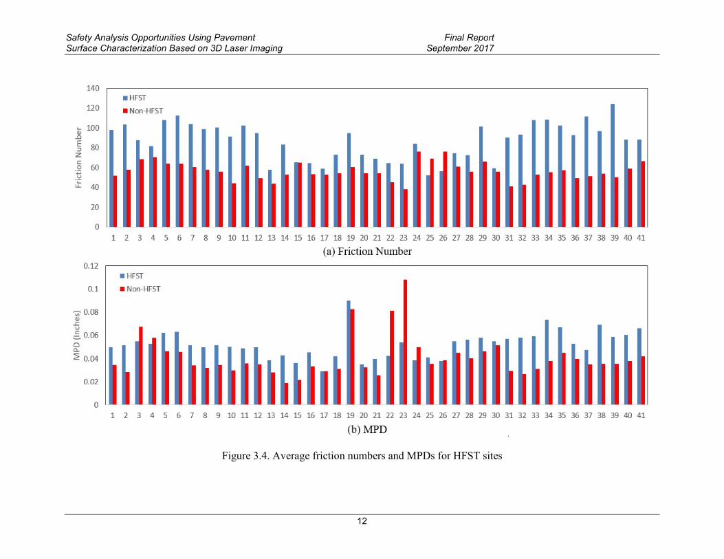
Safety Analysis Opportunities Using Pavement Final ReportSurface Characterization Based on 3D Laser Imaging September 2017
Model Verification and Improvement
In this model the effects of each independent variables (eg MPD) on dependent variables (eg FN) are assumed to be linear If the effects of the independent variables on the dependent variables appear to be non-linear this model may not be the appropriate fit for the data In this study the residual plots is used to investigate the linear effects of independent variable on the dependent variable The residual plot shows the residuals (the differences between the measured and predicted values) on the vertical axis and the independent variable on the horizontal axis If the points in a residual plot are randomly distributed around the horizontal axis a linear regression model may be appropriate for the data otherwise a non-linear model is more appropriate [48] Figure 415 shows the residual plots of the four variables
Note that the Figures 415b and 415d show a random dispersion around the horizontal axis indicating the linear models can be applied on these two variables to predict pavement friction Figures 415a and 415c show non-random patterns (U-shaped or inverted U-shaped) are observed for the Skewness and TAR indicating the non-linear models should be used for the two variables Based on Figure 416(a) a non-linear model should be developed to fit the FNs with the independent variable ldquoMPDrdquo After several trial-and-error a three-order polynomial model is employed with the largest R-squared value Similarly exponential model is developed for the SBI to fit the measured FNs as shown in Figure 416b Subsequently data transformation is performed
Figure 415 Residual plots of the four variablesa) MPD b) Skewness c) SBI d) TAR
34
Safety Analysis Opportunities Using Pavement Final ReportSurface Characterization Based on 3D Laser Imaging September 2017
Figure 416 Non-linear models a) MPD and b) SBI
In the subsequent multivariate analysis the original MPD and SBI are replaced by the transformed MPD and SBI calculated from the developed models and the multivariate regression analysis results are given in Table 43 Note that the p-values are approaching to the zero indicating the newly developed model are statistically more significant for pavement friction prediction As a result a new model can be developed with the four variables MPD Skewness TAR and SBI as mathematically described in Equation (412)
119865119873 = minus71415 119872119875119863ଷ + 225643119872119875119863ଶ minus 2264432119872119875119863 + 704119878119896119890119908119899119890119904119904 + 1343119879119860119877 +
589119890ଽସௌூ + 74393 (412)
Table 43 Multivariate regression results from Skewness TAR NEW_MPD and NEW_SBI
Indicator Coefficients Standard
Error t Stat P-value
Lower 95
Upper 95
Lower 950
Upper 950
Intercept -1564 468 -334 000 -2496 -632 -2496 -632
Skewness 704 118 596 000 469 939 469 939 TAR 1343 443 303 000 461 2226 461 2226 NEW_MPD 058 006 950 000 046 070 046 070
NEW_SBI 060 007 864 000 046 074 046 074
Correlation between the Predicted and Measured FNs
The measured FNs are correlated with the predicted FNs from the Equation 12 with an R-squared value of 0895 Apparently there are three outliers among the test samples due to their large deviations from the fitting line as illustrated in Figure 417a After the influences of the outliers on the developed models are eliminated a new linear model can be developed with an R-squared value of 0947 as shown in Figure 417b
As a result pavement friction can be estimated based on the four texture indicators MPD Skewness TAR and SBI MPD and Skewness belong to the amplitude parameters representing
35
Safety Analysis Opportunities Using Pavement Final ReportSurface Characterization Based on 3D Laser Imaging September 2017
surface height distribution TAR belongs to the spacing parameters describing pavement surface texture pattern SBI belongs to the functional parameters disclosing surface bearing capacity and pavement frictional properties
Figure 417 Correlation results between the predicted and measured FNsa) with outliers b) after outlier removal
36
Safety Analysis Opportunities Using Pavement Final ReportSurface Characterization Based on 3D Laser Imaging September 2017
5 EVALUATION OF PAVEMENT SURFACE HYDROPLANING
Introduction
Pavement hydroplaning occurs when water pressures build up in front of a moving tire resulting in an uplift force sufficient to separate the tire from the pavement The loss of steering and traction force produced during hydroplaning may cause the vehicle to lose control especially when a steering tire is involved [49] Past studies indicated the event of hydroplaning is highly associated with several factors including pavement texture cross slope longitudinal grade pavement width pavement types pavement condition tire characteristics and rainfall intensity [50 51]
Numerous field studies were dedicated to developing hydroplaning prediction models in the past decades [52] The models can be grouped into two categories empirical models and analytical models [53] The empirical methods use experimental data and equations to predict hydroplaning including Road Research Laboratory (RRL) equations to estimate water film depth (WFD) [54] National Aeronautics and Space Administration (NASA) models developed based on aircraft tire and airport pavement data (4) and Gallaway model to predict roadway hydroplaning [55] The analytical methods attempt to mathematically model hydroplaning of the sheet flow and its interaction with a tire including PAVDRN computer program developed by Pennsylvania State University [56] and the University of South Florida (USF) model based on Ong and Fwas numerical prediction [57]
Pavement slope also termed as flow path slope consists of cross slope and longitudinal grade which exerts a tremendous influence on hydroplaning prediction [58] To maintain constant water film hydroplaning simulation tests in past studies were conducted on pavements at tangent and flat terrain[59 60] For pavement segments with horizontal curve and severe down grade a smaller uplift force of water can cause hydroplaning issues due to the reduced vertical wheel load caused by large slopes However past studies on hydroplaning prediction neglected the influences of pavement slope on vertical wheel loads of vehicles The existing hydroplaning prediction models overestimate hydroplaning speed and are particularly not suitable to analyze pavements with steep pavement slope
Hydroplaning Prediction Models
Gallaway and USF Models
The Gallaway model is an empirical method developed by Gallaway et al [55] for the US Department of Transportation The method described in Equation (51)-(55) was adopted in the Texas Department of Transportation (TxDOT) Hydraulic Design Manual [55] The flow path an important factor on hydroplaning prediction model can be defined in Figure 51 and calculated with Equation (51) The USF model is an analytical hydroplaning prediction model developed at the University of South Florida based on Ong and Fwas comprehensive numerical prediction shown in Equation (56) The USF model can be used to predict the hydroplaning speeds for different light vehicles that employ tires compatible with the locked-wheel tester tires [57]
37
Safety Analysis Opportunities Using Pavement Final ReportSurface Characterization Based on 3D Laser Imaging September 2017
ଶ ଶ)ଵଶ S = (S୪ + Sୡ (51)
119871 = 119882 times (119878frasl119878) (52)
ସଷ ସଶ119882119865119863 = 001485(119872119879119863ଵଵ times 119871 times 119868ହଽ) (119878frasl )൧ minus 119872119879119863 (53)
ଵଶଷଽ ቀ ቁ + 350 ௐிబబల119860 = Max of ቐ (54)
ଶଶଷହଵ [ቀ ቁ minus 497] times 119872119879119863ଵସ ௐிబబల
119907 = 09143 times 119878119863ସ times 119875௧
ଷ times (119879119863 + 0794) times 119860 (55)
ଶ ହ 119907 = 119882ଶ times 119875௧ times [( ) + 049] (56)
ௐிబబల
Where WFD Water film depth (mm) MTD Mean texture depth (mm) calculated from the macro texture data v୮ Hydroplaning speed (kmh) L Pavement flow path length (m) Sୡ Cross slope (mm) S୪ Longitudinal grade (mm) W୮ Pavement width (m) I Rainfall intensity (mmhr) P୲ Inflation pressure (Kpa) SD Spin down ratio TD Tire tread depth (mm) W Wheel load (N)
Figure 51 Schematic diagram of cross slope longitudinal grade and flow path
Effects of Pavement Slope on Vertical Wheel Load
Typically cross slope or longitudinal grade would reduce the vertical wheel load of vehicles on pavement surface [61] Hydroplaning occurs when the vertical wheel load is equivalent to the uplift force by water (Equation (57)) and the steering and traction force would be lost during hydroplaning
Figure 52 (a) shows the pavement section with a large longitudinal grade When the vehicle travels on this pavement segment the vehicle gravity center would be partitioned into two components of forces one (wheel load) is perpendicular with the travelling surface and the other one (traction force) is parallel with pavement surface The wheel load would decrease with the increase of longitudinal grade (Equation (58)) and the reduced wheel load would increase the hydroplaning risk
38
Safety Analysis Opportunities Using Pavement Final ReportSurface Characterization Based on 3D Laser Imaging September 2017
Figure 52 (b) shows the pavement section with horizontal curves or large cross slope Similarly the vehicle gravity center is partitioned into two components of forces when the vehicle travels on the horizontal curve One component of force is the wheel load and the other one is the centripetal force shown in Figure 52 (b) The wheel load on horizontal curve would decrease with the increase of super-elevation (Equation (59)) Finally the wheel load can be calculated with flow path slope by combining the cross slope and longitudinal grade as given in Equation (510)
119865 = 119882 (57)
119882 = 119866 times 119888119900119904(β) (58)
119882 = 119866 times 119888119900119904(α) (59)
119882 = 119866 times 119888119900119904(ρ) (510)
Where F୮ -- Minimum uplift force causing hydroplaning (N) W -- Wheel load (N) W --Wheel load in longitudinal section (N) Wେ -- Wheel load in cross section (N) G -- Gravity of vehicle (N) β -- Angle of longitudinal grade (degree) α-- Angle of cross slope (degree) ρ -- Angle of flow path slope (degree)
Figure 52 Vehicle travelling on pavements with (a) longitudinal grade (b) horizontal curve
Improved Hydroplaning Speed Prediction Models
In the current models the influences of flow path slope on vertical wheel load are not taken into account in hydroplaning prediction models Therefore this study aims at improving the existing
39
Safety Analysis Opportunities Using Pavement Final ReportSurface Characterization Based on 3D Laser Imaging September 2017
Gallaway and USF models by considering the effects of flow path slope on wheel loads as shown in Equations (511) and (512)
119907 = 09143 times 119878119863ସ times (119875௧ times 119888119900119904120588)
ଷ times (119879119863 + 0794) times 119860 (511)
119907 = (119882 times 119888119900119904120588)ଶ times (119875௧ times 119888119900119904120588)
ହ times (082 frasl119882119865119863 + 049) (512)
Where W -- Wheel load (N) WFD -- Water film depth (mm) P୲ -- Inflation pressure (Kpa) SD -- Spin down ratio TD -- Tire tread depth (mm) A -- Maximum value of Equation (4) ρ -- Angle of flow path slope (degree)
Sensitivity Analysis of the Improved Models
To explore the sensitivity of cross slope and longitudinal grade on hydroplaning speed the cross slope and longitudinal grade change by plusmn 25 plusmn 50 and plusmn 75 individually while the other variables are maintained constant values The constant values of each factor is assumed to be the average values of that factor measured for test site as provided as follows Cross slope 119878 = 153 Rainfall intensity 119868 = 1484 119898119898ℎ119903 Mean texture depth MTD = 12 mm Longitudinal grade S୪ = 132
The results of sensitivity analysis from the improved Gallaway and USF models to cross slope and longitudinal grade are given in Figure 3 It can be seen that the resulting change in hydroplaning speed VP is apparent along the increase of cross slope and longitudinal grade In the two improved models the hydroplaning speed is affected by both the vertical load and the flow path length Typically the increase in cross slope or longitudinal grade would diminish the vertical wheel load The increase in cross slope would shorten the flow path length while the increase in longitudinal grades would extend the flow path length Both the decrease in vertical load and the increase in flow path length would reduce the hydroplaning speed
Accordingly the hydroplaning speed should decrease with the increase of longitudinal slope and may either increase or decrease with the increase of cross slope depending on effects of vertical load and flow paths Figure 53 shows that hydroplaning speed goes up with the increase of the cross slope indicating the effect of flow path length on hydroplaning speed is greater than that of wheel load It is shown that hydroplaning speed is more sensitive to the cross slope than longitudinal grade in the two improved models
40
Safety Analysis Opportunities Using Pavement Final ReportSurface Characterization Based on 3D Laser Imaging September 2017
Figure 53 Sensitivity of improved hydroplaning models (a) longitudinal grade (b) cross slope
Data Preparation
Estimated Mean Texture Depth (EMTD)
The methodologies for texture measurements can be grouped into two categories static and high-speed methods The static test methods include Sand Patch Method [26] Circular Track Meter [24] and Outflow Meter [62] and their measurements are conducted on the marked or specified small areas The traditional high-speed test techniques are characterized with the laser based data acquisition systems [63] with a spot laser resulting in a single line of measurement along the longitudinal direction of pavement The measurements are continuously conducted on test sections which can be regarded as an efficient tool for network level pavement survey
The widely used texture indicators include the Mean Profile Depth (MPD) and Mean Texture Depth (MTD) [25 26] In this study the MTD methodology is applied since the estimation of water film depth is dependent on the MTD in the hydroplaning models However as the manual process to obtain MTD through the Sand Patch Method is a standard time-consuming and somewhat not reliable enough [47] the 3D pavement surface captured with the 3D Ultra technology is therefore used as an alternative to be used as input to calculate area texture simulating the Sand Patch Method The alternative substantially improves data collection efficiency and reliability of computing surface texture As a volumetric method the Estimated MTD (EMTD) is therefore introduced in the research by simulating the Sand Patch Method with 1mm 3D laser imaging data of the entire lane as shown in Equation 513 [47] EMTD and MTD are assumed to be equivalent in the presented research
ವ సಾ స ∬ [ிబி(௫௬)]ௗ௫ௗ௬ sumసభ sumసభ [ிబி(௫௬)] బ 119864119872119879119863 = (1frasl119896) times sum = (1frasl119896) times sum (513) ୀଵ ୀଵ
Where 119865(119909 119910) ndash The pixel depth at point (x y) 119863 ndash The integral or gridded area containing of MtimesN pixels 119865 ndash The maximum peak in each area D 119870 ndash The number of grids within the test sample
41
Safety Analysis Opportunities Using Pavement Final ReportSurface Characterization Based on 3D Laser Imaging September 2017
Cross Slope Calibration
A properly designed and constructed cross slope is important for safe travelling since inadequate cross slopes may result in low efficiency in drainage and steep cross slopes may lead to vehicle maneuvering difficulties Therefore the accurate measurement of cross slope is important for hydroplaning speed prediction In this study 1mm 3D pavement data and IMU data are combined together to reproduce the cross slope of pavements
IMU mounted on the vehicle can measure three Euler angles which are termed as roll (Euler angle about x-axis) pitch (Euler angle about y-axis) and yaw (Euler angle about z-axis) respectively The roll angle is to represent pavement cross slope and pitch angle is traditionally used to represent pavement longitudinal grade based on the assumption that the vehicle floor is parallel with pavement surface during travelling However in real world the vehicle floor is not parallel with pavement surface during travelling which can be caused by 1) uneven gravity distribution of the vehicle 2) vibration of the vehicle during travelling 3) pavement surface geometry and condition
This study attempts to measure the vehicles body roll angle in X coordinate (angle γ) using the collected 3D laser imaging data Two sensors mounted on the rear of the DHDV are capable of covering the entire lane The ldquotruerdquo cross slope of pavements can be approximately determined with two parameters the tilt of the vehicle floor and the slope of pavement surface captured by 3D cameras [47] As Figure 54 shows the IMU system measures the angle θ of the vehicle relative to a level datum γ is the vehicle vibration angle in X coordinate which can be calculated in Equation (514) The true cross slope can be obtained by Equation (515) However in real world the angle θ and γ are very small so the cross slope can be directly computed as the difference in slope of θ and slope of γ (Equation (516)) [64]
୷మ୷భγ = act tan ( ) (514)
α = tan(θ + γ) (515)
α = tan(θ) + tan(γ) (516)
Where α ndash Angle of cross slope (degree) γ ndash The body roll angle of vehicle (degree) θ ndash IMU roll angle (degree) L ndash The distance between left and right laser (m) yଵ ndash The vertical distance from left sensor to the pavement surface (m) yଶ ndash The vertical distance from right sensor to the pavement surface (m)
42
Safety Analysis Opportunities Using Pavement Final ReportSurface Characterization Based on 3D Laser Imaging September 2017
Figure 54 Cross slope calibration based on IMU and 1mm 3D data
Software Interface for Automated Hydroplaning Prediction
A software program named Automated Hydroplaning Prediction Program (AHPP) is developed in this study to implement data processing and analysis Figure 55 shows the main interface of AHPP Once users import the IMU and 3D image data into AHPP the two types of data (1mm 3D laser imaging data and IMU data) can be automatically matched by Distance Measurement Instrument (DMI) pulses and the calibrated cross slope can be produced by the integration of IMU data and 3D data In AHPP users can manually assign the local rainfall intensity and pavement types The AHPP outputs include EMTD WFD calibrated cross slope longitudinal grade and predicted hydroplaning speeds from various models
Figure 55 Software interface for automated hydroplaning prediction
43
Safety Analysis Opportunities Using Pavement Final ReportSurface Characterization Based on 3D Laser Imaging September 2017
Case Study
Testing Site
A flexible pavement section located in Spavinaw Oklahoma is chosen as the test section which starts from the location (Latitude 36329175 Longitude -95081696) and ends with the location (Latitude 36351066 Longitude -95062796) with a length of 435 km The pavement of the test lane is in excellent condition and has a width of 365m On this test section there are five horizontal curves
Selection of Sample Size
The 3D laser imaging data collected with the 3D Ultra DHDV is stored on computer hard disk in the form of raw data files with the size of 4096 pixel wide by 2048 pixel long The raw data files are used as basic input data sets or samples and subsequently data processing and analysis are conducted on each individual sample In this study one raw image is considered as a sample (228m long) and the entire pavement section consists of 1915 samples
Local Rainfall Intensity
The local rainfall intensity at the test site is obtained from National Oceanic and Atmospheric Administrations (NOAA) National Water Service database [65] Table 51 shows the precipitation in Spavinaw Station Oklahoma from NOAA database The two-year return period storm with duration of five minutes is used in Gallaway and USF models for rainfall intensity acquisition Based on NOAA database the rainfall intensity of 1484mmhour is used for the test site
Table 51 Precipitation in Spavinaw station Duration Recurrence Recurrence Recurrence Recurrence (in mm) - 1 year - 2 year - 5 year - 10 year 5 min 1087 1237 1491 1704
10 min 1593 1811 2182 2497 15 min 1941 2209 2667 3048 30 min 2870 3277 3962 4547
Cross Slope and Longitudinal Grade
Both longitudinal grade and cross slope are the key factors to form flow path slope As Figure 56(a) shows the maximum longitudinal grade is 1203 and the standard deviation is 248 Due to the vibration of the surveying vehicle there is some noise in the raw cross slope captured by IMU roll angle Based on the 3D laser imaging data the vehicle body roll angle can be measured and then the raw cross slope is calibrated Figure 56(b) shows the raw cross slope and calibrated cross slopes Comparing the raw cross slope data and calibrated cross slope the majority of the noise is eliminated from the raw data through the calibration The cross slope presents negative values at left turn curves and positive values at right turn curves In this test site curves 1 4 and 5 belong to left turn curve while curves 2 and 3 belong to right turn curve The statistical results of the calibrated cross slopes on test site are given as follows (1) the
44
Safety Analysis Opportunities Using Pavement Final ReportSurface Characterization Based on 3D Laser Imaging September 2017
average cross slope on the straight road segments is 194 (2) the average cross slope of curve 1 2 3 4 and 5 are -206 496 580 -381 and -501 respectively
Figure 56 Pavement geometry of the testing site (a) Longitudinal grade (b) Cross slope
EMTDs and WFDs
Figure 57(a) shows the corresponding WFD along the test section with an average value of 173mm and the maximum value of 852 mm and Figure 57(b) shows the EMTDs at the test section with an average value of 120 mm The WFD is calculated with Gallaway WFD model based on pavement texture depth flow path slope and local rainfall intensity as inputs
Figure 57 WFDs and EMTDs of test site (a) WFDs (b) EMTDS
45
Safety Analysis Opportunities Using Pavement Final ReportSurface Characterization Based on 3D Laser Imaging September 2017
Hydroplaning Speed Estimation
15 samples of the calculated WFD EMTD and IMU data for hydroplaning speed prediction are given in Table 52 Gallaway model USF model the improved Gallaway model and the improved USF model are utilized to predict hydroplaning speed respectively as shown in Figure 10(a) Results indicate the predicted hydroplaning speeds from original Gallaway and USF model are approximately 140kmh and 165kmh respectively which are around 50kmh higher than those predicted from the improved Gallaway model (96kmh) and improved USF model (91kmh) The results also show as expected that the hydroplaning speeds at curves of the five horizontal curves in Figure 58(a) are lower than that on the straight road sections
Table 52 Sample 3D and IMU data for hydroplaning speed calculation Sample ID WFD (mm) EMTD (mm) Cross Slope () Longitudinal Grade ()
1 164 112 207 327 2 151 111 226 318 3 135 111 254 310 4 130 110 268 312 5 123 111 282 307 6 121 109 287 289 7 113 112 295 278 8 105 117 305 277 9 103 114 323 272 10 100 110 344 267 11 093 112 364 271 12 094 111 374 281 13 094 110 376 285 14 086 117 379 279 15 092 110 383 276
Potential Hydroplaning Segment Detection
Identification of locations with hydroplaning potential is based on the comparison of estimated hydroplaning speed with posted speed of the road section [47] At the test site speed limits are 80kmh on straight sections and 56kmh on road curves The average hydroplaning speeds calculated with the four models are used to detect potential hydroplaning segments shown in Figure 58(a) Since the predicted hydroplaning speeds at the five curves are higher than posted speed limit there is a low hydroplaning risk at the five curves for vehicles operating at speed limit However for several segments of the test site the predicted hydroplaning speeds are lower than the posted speed limit Therefore these segments can be identified as potential segments for increased hydroplaning risk as marked with red line in Figure 58(b) To minimize traffic crashes caused by hydroplaning highway agencies can post a reduced speed sign at these locations or take other remedial actions such as installing High-Friction Surface Treatment (HFST) [66]
46
Safety Analysis Opportunities Using Pavement Final ReportSurface Characterization Based on 3D Laser Imaging September 2017
Figure 58 Detection of potential hydroplaning risk (a) hydroplaning speed (b) increased hydroplaning potential segments
47
Safety Analysis Opportunities Using Pavement Final ReportSurface Characterization Based on 3D Laser Imaging September 2017
6 SUMMARY
The 3D Ultra laser imaging technology has the capability to collect pavement surface texture data at full-lane coverage at 1 mm resolution in all three dimensions at speed up to 60MPH This single-pass and complete lane coverage platform provides an ideal solution to evaluate pavement surface characteristics for safety analysis and many different data collection needs without interrupting traffic Furthermore it will saved cost by eliminating the need for maintenance of traffic
In this study the 3D Ultra laser imaging technology with necessary software tools are utilized for data collection and subsequent surface characterization and safety evaluation and analysis First the 1mm 3D data for 21 HFST sites in 11 states with a total of 41 sections are collected for each traffic lane at the posted highway speeds Pavement rutting and macro-texture data are calculated from collected 1mm 3D data sets while pavement friction data are collected using FHWAs fixed-slip continuous friction tester The measured surface characteristics on the HFST sites and untreated existing pavements are compared and paired t-tests are performed to determine the effectiveness of the HFST sites in improving surface characteristics It is evident that the HFST surfaces have statistically significant higher friction numbers and surface macro-texture MPD values than those on the adjacent pavements without HFST There exist several exceptions to such trend 2 sections for friction data and 5 sections for MPD data Multivariate analyses are conducted to investigate the impacts of five independent variables precipitation average temperature HFST installation age aggregate type and AADT on HFST friction performance Average temperature and HFST installation age are identified to have significantly impact on friction performance of HFST (FNHFST) and the ratio of friction on HFST to that on non-HFST (FN Ratio) Based on the trend between FN Ratio and installation age in general the benefit of HFST in friction effectiveness is lost after approximate 60 months (5 years) of service HFST sites using calcined bauxite aggregates exhibit higher friction performance than those using flints The regressional friction prediction models are therefore developed for HFST which can be used to predict the service life of HFST installation and aid decision making within a highway agency However it should be noted that the models donrsquot consider the pavement conditions before HFST application and HFST construction quality variations as the dependent variables due to the unavailability of data In addition detailed traffic data for ramps and each lane of sites with multiple lanes are not available and have to be estimated during the model development
Surface texture and friction are two primary characteristics for pavement safety evaluation Understanding their relationship is critical to reduce potential traffic crashes especially at wet conditions However the currently used texture indicators such as Mean Profile Depth (MPD) and Mean Texture Depth (MTD) are calculated restricted on either a small portion on pavement surface or single line of profile measurement and thus only reveal partial aspects of texture property With 1mm 3D laser texture data eight surface texture indicators are examined for their applications on pavement friction prediction The eight surface texture indicators are grouped into four categories amplitude parameters (including MPD SMTD RMS Skewness and Kurtosis) spacing parameters (TAR) hybrid parameters (SAR) and functional parameters (SBI) To avoid using two highly correlated texture indicators in the friction prediction model correlation analyses are conducted and found that 1) SMTD are highly correlated with MPD 2)
48
Safety Analysis Opportunities Using Pavement Final ReportSurface Characterization Based on 3D Laser Imaging September 2017
RMS is highly correlated with SAR As a result six texture indicators including MPD Skewness Kurtosis TAR SAR and SBI are adopted for the development of pavement friction prediction model using multivariate regression analysis The developed model can be used to predict pavement friction based on various texture indicators and may be beneficial in the continuous measurement and evaluation of pavement safety for the project- and network- level pavement surveys
The third application of using 1mm 3D Ultra data sets is to predict and evaluate pavement surface hydroplaning risk Considering the effects of flow path slope on vertical wheel load perpendicular to pavement surface and the resulting hydroplaning speed the Gallaway and USF models are modified for improvements in this study The sensitivity analysis shows that the hydroplaning speed is more sensitive to cross slope than longitudinal grade in the improved models A 3D based volumetric measuring method is used to calculate the estimated MTD based on the full-lane 1mm 3D data Subsequently IMU data and 3D data are combined to model vehicle movements on cross slopes Local rainfall intensity is obtained from NOAA precipitation database By considering effects of cross slope and longitudinal grade on wheel load and flow path length it is found that hydroplaning speed decreases with the increase of the longitudinal grade but increases with the increase of the cross slope The improved models predict lower hydroplaning speed than that from the original Gallaway and USF models An important future work is to use a combined slope based on longitudinal grade and cross slope to demonstrate the validity and effectiveness of the improved models
This study with field pavement applications has shown that the 1mm 3D Ultra which represent a form of 3D Laser imaging technology is promising in real-time pavement surface characterization and evaluation for both pavement and safety management at network and project level surveys It is anticipated that more data collection with more testing sites are to be performed to validate the new emerging 3D laser imaging technology as a single-pass and complete lane-coverage platform for multiple safety and pavement evaluation purposes In addition the long-term monitoring of the HFTS sites in multiple states is highly recommended due to the need to determine multi-year performance of the HFTS applications in terms of region pavement condition materials used geometric properties and other factors The recommended long-term study would provide much needed data for both design and construction of HFTS for its widespread adoption
49
Safety Analysis Opportunities Using Pavement Final ReportSurface Characterization Based on 3D Laser Imaging September 2017
REFERENCES
[1] Brimley B and Carlson P Using High Friction Surface Treatments to Improve Safety at Horizontal Curves Texas Transportation Institute httpd2dtl5nnlpfr0rcloudfrontnetttitamuedudocumentsTTI-2012-8pdf 2012 (accessed 150625)
[2] The Trans Tec Group INC Welcome to High Friction Roads httpwwwhighfrictionroadscom 2015 (accessed 150725)
[3] Bledsoe J Missouri Demonstration Project The Use of High-Friction Surface Treatments on Missouri Highways FHWA US Department of Transportation httpplan4operationsdotgovhflsummarypdf_2Missouri20High20Friction20Report 20draft20Finalpdf 2015 (accessed 150630)
[4] Moravec M High Friction Surface Treatments at High-Crash Horizontal Curves Arizona PavementsMaterials Conference Phoenix AZ httpwwwintransiastateedueventsmidcon2013documentspresentation-submissions3-C_61_08142013pdf 2013 (accessed 150630)
[5] South Dakota Department of Transportation (SDDOT) Accelerated Innovation Deployment (AID) Demonstration Project High Friction Surface Treatment httpwwwfhwadotgovacceleratinggrantspdfsSD_2014_AID_Grantpdf 2015 (accessed 150611)
[6] Bischoff D Investigative Study of the Italgrip TM System WI-04-08 Wisconsin Department of Transportation Madison WI httpwisdotresearchwigovwp-contentuploadswi-04-08italgrippdf 2008 (accessed 150620)
[7] Izeppi E Flintsch G and McGhee K Field Performance of High Friction Surfaces Publication FHWAVTRC 10-CR6 FHWA US Department of Transportation httpwwwvirginiadotorgvtrcmainonline_reportspdf10-cr6pdf 2010 (accessed 150615)
[8] Waters J High Friction Surfacing Failure Mechanisms 3rd International Surface Friction Conference Safer Road Surfaces ndash Saving Lives Gold Coast Australia 2011
[9] Wang Kelvin C P Elements of Automated Survey of Pavements and a 3D Methodology J mod transp Vol 19 pp 51-57 2011
[10] AASTHO Quantifying cracks in asphalt pavement surfaces from collected images utilizing automated methods AASHTO Designation PP67-10 American Association of State Highway and Transportation Officials Washington DC 2013
[11] AASTHO 2013 Standard Practice for Determining Pavement Deformation Parameters and Cross Slope from Collected Transverse Profiles AASHTO Designation PP69-10 American Association of State Highway and Transportation Officials Washington DC 2013
[12] Hall J W Smith K L Titus-Glover L Wambold J C Yager T J and Rado Z Guide for Pavement Friction Final Report for NCHRP Project 01-43 National Cooperative
50
Safety Analysis Opportunities Using Pavement Final ReportSurface Characterization Based on 3D Laser Imaging September 2017
Highway Research Program (NCHRP) Transportation Research Board (TRB) Washington DC 2009
[13] Ahammed MA and Tighe SL Concrete Pavement Surface Textures and Multivariables Frictional Performance Analysis a North American Case Study Can J Civil Eng Vol 35 727-738 2008
[14] Ergun M Iyinam S and Iyinam AF Prediction of Road Surface Friction Coefficient Using Only Macro- and Microtexture Measurements J Transp Eng Vol 131 pp 311-319 2005
[15] Flintsch GW et al The Little Book of Tire Pavement Friction Pavement Surface Properties Consortium httpssecurehostingvteduwwwappsvttivtedu1-pagersCSTI_FlintschThe20Little20Book20of20Tire20Pavement20Frictionpdf 2012 (accessed 150501)
[16] Henry J J NCHRP Synthesis 291 Evaluation of Pavement Friction Characteristics TRB National Research Council Washington DC 2000
[17] Ahammed MA and Tighe SL Effect of Short-term and Long-term Weather on Pavement Surface Friction Int J Na Res Tech Vol 3 pp 295-302 2010
[18] Luo Y Effect of Pavement Temperature on Frictional Properties of Hot-Mix-Asphalt Pavement Surfaces at the Virginia Smart Road MS Thesis Virginia Polytechnic Institute and State University Blacksburg Va 2003
[19] Fuents L G Investigation of the Factors Influencing Skid Resistance and the International Friction Index PhD Thesis University of South Florida Tampa FL 2009
[20] American Society for Testing and Materials (ASTM) ASTM E 867 Standard Terminology Relating to Vehicle-Pavement Systems ASTM Standard Practice E 867 Book of ASTM Standards Volume 0403 Philadelphia P A 2011
[21] International Standards Organization (ISO) Characterization of Pavement Texture using Surface Profiles ndash Part 1 Determination of Mean Profile Depth Acoustics ISO Standard 13473 International Standards Organization Geneva Switzerland 1998
[22] PIARC World Road Association Report of the Committee on Surface Characteristics In Proceeding of XVIII World Road Congress Brussels Belgium pp 13ndash19 1987
[23] Sandburg U Influence of Road Surface Texture on Traffic Characteristics Related to Environment Economy and Safety A State-of-the-Art Study Regarding Measures and Measuring Methods VTI Report 53A-1997 Swedish National Road Administration Borlange Sweden 1998
[24] American Society for Testing and Materials (ASTM) ASTM E 2157 Standard Test Method for Measuring Pavement Macro texture Properties Using the Circular Track Meter ASTM Standard Practice E 2157 Book of ASTM Standards Volume 0403 Philadelphia P A 2011
51
Safety Analysis Opportunities Using Pavement Final ReportSurface Characterization Based on 3D Laser Imaging September 2017
[25] American Society for Testing and Materials (ASTM) ASTM E 1845 Calculating Pavement Macro texture Profile Depth ASTM Standard Practice E 1845 Book of ASTM Standards Volume 0403 Philadelphia P A 2011
[26] American Society for Testing and Materials (ASTM) ASTM E 965 Standard Test Method for Measuring Pavement Macro texture Depth Using a Volumetric Technique ASTM Standard Practice E 965 Book of ASTM Standards Volume 0403 Philadelphia P A 2011
[27] McGhee K K amp Flintsch G W High-speed Texture Measurement of Pavements Virginia Transportation Research Council Charlottesville VA 2003
[28] Prowell B amp Hanson D Evaluation of Circular Texture Meter for Measuring Surface Texture of Pavements Transportation Research Record Journal of the Transportation Research Board No 1929 pp 88-96 2005
[29] Alvarez L amp Morel J M Formalization and Computational Aspects of Image Analysis Acta numerica Vol 3 pp 1-59 1994
[30] Gendy A E amp Shalaby A Mean Profile Depth of Pavement Surface Macrotexture Using Photometric Stereo Techniques Journal of Transportation Engineering Vol 133 No 7 pp 433-440 2007
[31] Kokkalis A and Panagouli O Fractal Evaluation of Pavement Skid Resistance Variations I Surface Wetting Chaos Solitons amp Fractals pp 1875-1890 1998
[32] American Society for Testing and Materials (ASTM) ASTM E 274 Standard Test Method for Skid Resistance of Paved Surfaces Using a Full-Scale Tire ASTM Standard Practice E 274 Book of ASTM Standards Volume 0403 Philadelphia P A 2011
[33] American Society for Testing and Materials (ASTM) ASTM E 303 Standard Test Method for Measuring Surface Frictional Properties Using a British Pendulum Tester ASTM Standard Practice E 303 Book of ASTM Standards Volume 0403 Philadelphia P A 2011
[34] Janoo VC and Horhonen C Performance Testing of Hot-Mix Asphalt Aggregates Special Report pp 99-20 1999
[35] Kuennen T Creating Friction Where Rubber Meets the Road Better Roads Vol 73 No 10 2003
[36] Leu MC Henry JJ Prediction of skid resistance as a function of speed from pavement texture measurements Transportation Research Record No 666 pp 7-13 1978
[37] Yager T J and Buhlmann F Macrotexture and Drainage Measurements on a Variety of Concrete and Asphalt Surfaces Pavement Surface Characteristics and Materials ASTM STP 763 pp 16-30 1982
[38] Rado Z Analysis of Texture Models PTI Report No 9510 Pennsylvania Transportation Institute (PTI) Penn State University State College Pennsylvania 1994
52
Safety Analysis Opportunities Using Pavement Final ReportSurface Characterization Based on 3D Laser Imaging September 2017
[39] Fwa T F Choo Y S and Liu Y (2003) Effect of Aggregate Spacing on Skid Resistance of Asphalt Pavement Journal of Transportation Engineering Vol 129 No 4 pp 420-426 2003
[40] Olek J Weiss W J and Garcia-Villarreal R Relating Surface Texture of Rigid Pavement with Noise and Skid Resistance Purdue University West Lafayette Indiana Report No SQDH-2004-1 (Final Report HL 2004-1) 2004
[41] Do MT Marsac P Delanne Y Prediction of Tirewet Road Friction from Road Surface Microtexture and Tire Rubber Properties In 5th International Symposium on Pavement Surface Characteristics Toronto 2004
[42] Ergun M Iyinam S amp Iyinam A F (2005) Prediction of Road Surface Friction Coefficient Using only Macro- and Micro texture Measurement Journal of transportation engineering Vol 131 No 4 pp 311-319 2005
[43] Kebrle J Walker R Texture measurement and friction estimation using laser data acquisition and neural networks In Proceedings of the 9th WSEAS International Conference on Mathematical and Computational Methods in Science and Engineering Trinidad and Tobago 2007
[44] Rezaei A Masad E Chowdhury A amp Harris P Predicting Asphalt Mixture Skid Resistance by Aggregate Characteristics and Gradation Transportation Research Record Journal of the Transportation Research Board No 2014 pp 24-33 2009
[45] American National Standards Institute Surface texture surface roughness waviness and lay American Society of Mechanical Engineers 1986
[46] Stout K J Sullivan PJ Dong WP Mainsah E Luo N Mathia T and Zahyouani H The development of methods for the characterization of roughness in three dimensions Commission of the European Communities 1993
[47] Luo Wenting Wang Kelvin C P Li Lin 2014 Surface Drainage Evaluation for Rigid Pavements Using IMU and 1 mm 3D Texture Data Transportation Research Record Journal of the Transportation Research Board Washington DC Pavement Management 2014 Volume 3 pp 121ndash128 2014
[48] Tsai C L Cai Z amp Wu X (1998) The examination of residual plots Statistica Sinica Vol 8 pp 445-465 1998
[49] Kumar SSantosh Anupam Kumar and FWA TF Analyzing effect of tire groove patterns on hydroplaning speed Journal of the Eastern Asia Society for Transportation Studies Vol 8 2009
[50] Khedr Safwan A and Breakah Tamer M Rutting parameters for asphalt concrete for different aggregate structures International Journal of Pavement Engineering Volume 12 Issue 1 pp 13-23 2011
53
Safety Analysis Opportunities Using Pavement Final ReportSurface Characterization Based on 3D Laser Imaging September 2017
[51] MISH Rohit Goyal Design and Analysis of Interceptor DrainsmdashEffect of Parameters ISH Journal of Hydraulic Engineering Volume 9 Issue 1 pp 61-71 2003
[52] Horne WB and RC Dreher Phenomena of Pneumatic Tire Hydroplaning NASA TN D-2-56 NASA Langley Research center NASA Hampton VA 1963
[53] Chesterton John Nancekivell Noel and Tunnicliffe Noel The use of the Gallaway Formula for Aquaplaning Evaluation in New Zealand Transit New Zealand and New Zealand Institute of Highway Technology (NZIHT) 8thAnnual Conference 2006
[54] Russam K and Ross NF The Depth of Rain Water on Road Surfaces Road Research Laboratory Ministry of Transport Report No LR 236 pp25 1968
[55] Gallaway B M et al Pavement and Geometric Design Criteria for Minimizing Hydroplaning Federal Highway Administration Report No FHWA-RD-79-31 1979
[56] Huebner RS et al PAVDRN Computer Model for Predicting Water Film Thickness and Potential or Hydroplaning on New and Reconditioned Pavements Transport Research Record 1599 pp 128-131 1996
[57] Gunaratne M Lu Q Yang J Hydroplaning on Multi Lane Facilities Report for Florida Department of Transportation Report No BDK84 977-14 2012
[58] Zhang Zhongjie Abu-Farsakh Murad Y and Tao Mingjiang Evaluation of trench backfills at highway cross-drains International Journal of Pavement Engineering Volume 6 Issue 2 pp77-87 2005
[59] Gallaway B M and Rose Gerry The Effects of Rainfall Intensity Pavement Cross Slope Surface Texture and Drainage Length on Pavement Water Depths Texas Transportation Institute Research Report No 138-5 1971
[60] Ong GP and Fwa TF Wet-pavement hydroplaning risk and skid-resistance Modeling ASCE Journal of Transportation Engineering Vol 133 No 10 2007
[61] Shafabakhsh GA Kashi E Effect of Aircraft Wheel Load and Configuration on Runway Damages Period Polytech Civil Eng Vol 59 No 1 pp 85-94 2015
[62] ASTM Measuring Pavement Texture Drainage Using an Outflow ASTM Standard Practice E 2380 Book of ASTM Standards Volume 0403 Philadelphia P A 2006
[63] ASTM Measuring Surface Frictional Properties Using the British Pendulum Tester ASTM Standard Practice E 303 Book of ASTM Standards Volume 0403 Philadelphia P A 2006
[64] Mekemson et al Method and Apparatus for Pavement Cross-slope Measurement Patent Application Publication Pub No US 20020013644 A1 2002
54
Safety Analysis Opportunities Using Pavement Final ReportSurface Characterization Based on 3D Laser Imaging September 2017
[65] NOAAs National Water Service Hydrometeorological Design Studies Center Precipitation Frequency Data Server (PFDS) httpdippernwsnoaagovhdscpfds Accessed on July 2014
[66] Shah Yogesh U Jain SS and Parida Manoranjan Evaluation of prioritization methods for effective pavement maintenance of urban roads International Journal of Pavement Engineering Volume 15 Issue 3 pp 238-250 2014
55
For More Information
Safety Analysis Opportunities Using Pavement Surface Characterization
Based on 3D Laser Imaging visit httpsafetyfhwadotgov
July 2017 FHWA-SA-17-046
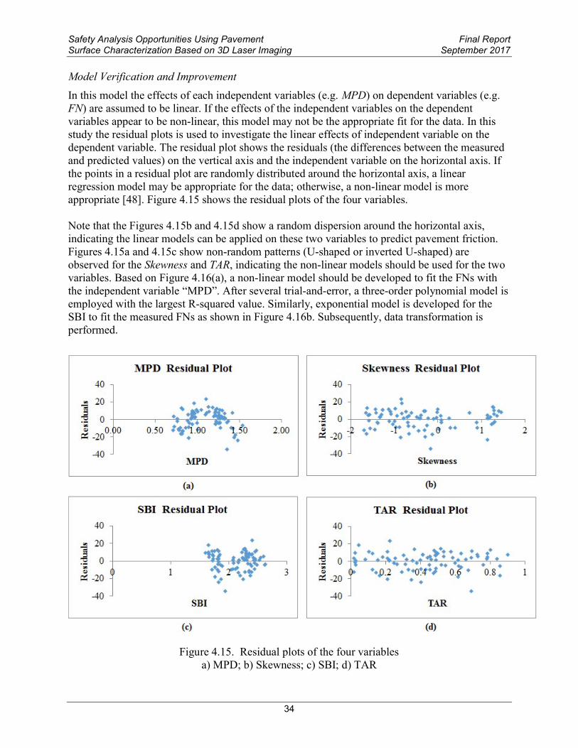
Safety Analysis Opportunities Using Pavement Final ReportSurface Characterization Based on 3D Laser Imaging September 2017
Figure 52 (b) shows the pavement section with horizontal curves or large cross slope Similarly the vehicle gravity center is partitioned into two components of forces when the vehicle travels on the horizontal curve One component of force is the wheel load and the other one is the centripetal force shown in Figure 52 (b) The wheel load on horizontal curve would decrease with the increase of super-elevation (Equation (59)) Finally the wheel load can be calculated with flow path slope by combining the cross slope and longitudinal grade as given in Equation (510)
119865 = 119882 (57)
119882 = 119866 times 119888119900119904(β) (58)
119882 = 119866 times 119888119900119904(α) (59)
119882 = 119866 times 119888119900119904(ρ) (510)
Where F୮ -- Minimum uplift force causing hydroplaning (N) W -- Wheel load (N) W --Wheel load in longitudinal section (N) Wେ -- Wheel load in cross section (N) G -- Gravity of vehicle (N) β -- Angle of longitudinal grade (degree) α-- Angle of cross slope (degree) ρ -- Angle of flow path slope (degree)
Figure 52 Vehicle travelling on pavements with (a) longitudinal grade (b) horizontal curve
Improved Hydroplaning Speed Prediction Models
In the current models the influences of flow path slope on vertical wheel load are not taken into account in hydroplaning prediction models Therefore this study aims at improving the existing
39
Safety Analysis Opportunities Using Pavement Final ReportSurface Characterization Based on 3D Laser Imaging September 2017
Gallaway and USF models by considering the effects of flow path slope on wheel loads as shown in Equations (511) and (512)
119907 = 09143 times 119878119863ସ times (119875௧ times 119888119900119904120588)
ଷ times (119879119863 + 0794) times 119860 (511)
119907 = (119882 times 119888119900119904120588)ଶ times (119875௧ times 119888119900119904120588)
ହ times (082 frasl119882119865119863 + 049) (512)
Where W -- Wheel load (N) WFD -- Water film depth (mm) P୲ -- Inflation pressure (Kpa) SD -- Spin down ratio TD -- Tire tread depth (mm) A -- Maximum value of Equation (4) ρ -- Angle of flow path slope (degree)
Sensitivity Analysis of the Improved Models
To explore the sensitivity of cross slope and longitudinal grade on hydroplaning speed the cross slope and longitudinal grade change by plusmn 25 plusmn 50 and plusmn 75 individually while the other variables are maintained constant values The constant values of each factor is assumed to be the average values of that factor measured for test site as provided as follows Cross slope 119878 = 153 Rainfall intensity 119868 = 1484 119898119898ℎ119903 Mean texture depth MTD = 12 mm Longitudinal grade S୪ = 132
The results of sensitivity analysis from the improved Gallaway and USF models to cross slope and longitudinal grade are given in Figure 3 It can be seen that the resulting change in hydroplaning speed VP is apparent along the increase of cross slope and longitudinal grade In the two improved models the hydroplaning speed is affected by both the vertical load and the flow path length Typically the increase in cross slope or longitudinal grade would diminish the vertical wheel load The increase in cross slope would shorten the flow path length while the increase in longitudinal grades would extend the flow path length Both the decrease in vertical load and the increase in flow path length would reduce the hydroplaning speed
Accordingly the hydroplaning speed should decrease with the increase of longitudinal slope and may either increase or decrease with the increase of cross slope depending on effects of vertical load and flow paths Figure 53 shows that hydroplaning speed goes up with the increase of the cross slope indicating the effect of flow path length on hydroplaning speed is greater than that of wheel load It is shown that hydroplaning speed is more sensitive to the cross slope than longitudinal grade in the two improved models
40
Safety Analysis Opportunities Using Pavement Final ReportSurface Characterization Based on 3D Laser Imaging September 2017
Figure 53 Sensitivity of improved hydroplaning models (a) longitudinal grade (b) cross slope
Data Preparation
Estimated Mean Texture Depth (EMTD)
The methodologies for texture measurements can be grouped into two categories static and high-speed methods The static test methods include Sand Patch Method [26] Circular Track Meter [24] and Outflow Meter [62] and their measurements are conducted on the marked or specified small areas The traditional high-speed test techniques are characterized with the laser based data acquisition systems [63] with a spot laser resulting in a single line of measurement along the longitudinal direction of pavement The measurements are continuously conducted on test sections which can be regarded as an efficient tool for network level pavement survey
The widely used texture indicators include the Mean Profile Depth (MPD) and Mean Texture Depth (MTD) [25 26] In this study the MTD methodology is applied since the estimation of water film depth is dependent on the MTD in the hydroplaning models However as the manual process to obtain MTD through the Sand Patch Method is a standard time-consuming and somewhat not reliable enough [47] the 3D pavement surface captured with the 3D Ultra technology is therefore used as an alternative to be used as input to calculate area texture simulating the Sand Patch Method The alternative substantially improves data collection efficiency and reliability of computing surface texture As a volumetric method the Estimated MTD (EMTD) is therefore introduced in the research by simulating the Sand Patch Method with 1mm 3D laser imaging data of the entire lane as shown in Equation 513 [47] EMTD and MTD are assumed to be equivalent in the presented research
ವ సಾ స ∬ [ிబி(௫௬)]ௗ௫ௗ௬ sumసభ sumసభ [ிబி(௫௬)] బ 119864119872119879119863 = (1frasl119896) times sum = (1frasl119896) times sum (513) ୀଵ ୀଵ
Where 119865(119909 119910) ndash The pixel depth at point (x y) 119863 ndash The integral or gridded area containing of MtimesN pixels 119865 ndash The maximum peak in each area D 119870 ndash The number of grids within the test sample
41
Safety Analysis Opportunities Using Pavement Final ReportSurface Characterization Based on 3D Laser Imaging September 2017
Cross Slope Calibration
A properly designed and constructed cross slope is important for safe travelling since inadequate cross slopes may result in low efficiency in drainage and steep cross slopes may lead to vehicle maneuvering difficulties Therefore the accurate measurement of cross slope is important for hydroplaning speed prediction In this study 1mm 3D pavement data and IMU data are combined together to reproduce the cross slope of pavements
IMU mounted on the vehicle can measure three Euler angles which are termed as roll (Euler angle about x-axis) pitch (Euler angle about y-axis) and yaw (Euler angle about z-axis) respectively The roll angle is to represent pavement cross slope and pitch angle is traditionally used to represent pavement longitudinal grade based on the assumption that the vehicle floor is parallel with pavement surface during travelling However in real world the vehicle floor is not parallel with pavement surface during travelling which can be caused by 1) uneven gravity distribution of the vehicle 2) vibration of the vehicle during travelling 3) pavement surface geometry and condition
This study attempts to measure the vehicles body roll angle in X coordinate (angle γ) using the collected 3D laser imaging data Two sensors mounted on the rear of the DHDV are capable of covering the entire lane The ldquotruerdquo cross slope of pavements can be approximately determined with two parameters the tilt of the vehicle floor and the slope of pavement surface captured by 3D cameras [47] As Figure 54 shows the IMU system measures the angle θ of the vehicle relative to a level datum γ is the vehicle vibration angle in X coordinate which can be calculated in Equation (514) The true cross slope can be obtained by Equation (515) However in real world the angle θ and γ are very small so the cross slope can be directly computed as the difference in slope of θ and slope of γ (Equation (516)) [64]
୷మ୷భγ = act tan ( ) (514)
α = tan(θ + γ) (515)
α = tan(θ) + tan(γ) (516)
Where α ndash Angle of cross slope (degree) γ ndash The body roll angle of vehicle (degree) θ ndash IMU roll angle (degree) L ndash The distance between left and right laser (m) yଵ ndash The vertical distance from left sensor to the pavement surface (m) yଶ ndash The vertical distance from right sensor to the pavement surface (m)
42
Safety Analysis Opportunities Using Pavement Final ReportSurface Characterization Based on 3D Laser Imaging September 2017
Figure 54 Cross slope calibration based on IMU and 1mm 3D data
Software Interface for Automated Hydroplaning Prediction
A software program named Automated Hydroplaning Prediction Program (AHPP) is developed in this study to implement data processing and analysis Figure 55 shows the main interface of AHPP Once users import the IMU and 3D image data into AHPP the two types of data (1mm 3D laser imaging data and IMU data) can be automatically matched by Distance Measurement Instrument (DMI) pulses and the calibrated cross slope can be produced by the integration of IMU data and 3D data In AHPP users can manually assign the local rainfall intensity and pavement types The AHPP outputs include EMTD WFD calibrated cross slope longitudinal grade and predicted hydroplaning speeds from various models
Figure 55 Software interface for automated hydroplaning prediction
43
Safety Analysis Opportunities Using Pavement Final ReportSurface Characterization Based on 3D Laser Imaging September 2017
Case Study
Testing Site
A flexible pavement section located in Spavinaw Oklahoma is chosen as the test section which starts from the location (Latitude 36329175 Longitude -95081696) and ends with the location (Latitude 36351066 Longitude -95062796) with a length of 435 km The pavement of the test lane is in excellent condition and has a width of 365m On this test section there are five horizontal curves
Selection of Sample Size
The 3D laser imaging data collected with the 3D Ultra DHDV is stored on computer hard disk in the form of raw data files with the size of 4096 pixel wide by 2048 pixel long The raw data files are used as basic input data sets or samples and subsequently data processing and analysis are conducted on each individual sample In this study one raw image is considered as a sample (228m long) and the entire pavement section consists of 1915 samples
Local Rainfall Intensity
The local rainfall intensity at the test site is obtained from National Oceanic and Atmospheric Administrations (NOAA) National Water Service database [65] Table 51 shows the precipitation in Spavinaw Station Oklahoma from NOAA database The two-year return period storm with duration of five minutes is used in Gallaway and USF models for rainfall intensity acquisition Based on NOAA database the rainfall intensity of 1484mmhour is used for the test site
Table 51 Precipitation in Spavinaw station Duration Recurrence Recurrence Recurrence Recurrence (in mm) - 1 year - 2 year - 5 year - 10 year 5 min 1087 1237 1491 1704
10 min 1593 1811 2182 2497 15 min 1941 2209 2667 3048 30 min 2870 3277 3962 4547
Cross Slope and Longitudinal Grade
Both longitudinal grade and cross slope are the key factors to form flow path slope As Figure 56(a) shows the maximum longitudinal grade is 1203 and the standard deviation is 248 Due to the vibration of the surveying vehicle there is some noise in the raw cross slope captured by IMU roll angle Based on the 3D laser imaging data the vehicle body roll angle can be measured and then the raw cross slope is calibrated Figure 56(b) shows the raw cross slope and calibrated cross slopes Comparing the raw cross slope data and calibrated cross slope the majority of the noise is eliminated from the raw data through the calibration The cross slope presents negative values at left turn curves and positive values at right turn curves In this test site curves 1 4 and 5 belong to left turn curve while curves 2 and 3 belong to right turn curve The statistical results of the calibrated cross slopes on test site are given as follows (1) the
44
Safety Analysis Opportunities Using Pavement Final ReportSurface Characterization Based on 3D Laser Imaging September 2017
average cross slope on the straight road segments is 194 (2) the average cross slope of curve 1 2 3 4 and 5 are -206 496 580 -381 and -501 respectively
Figure 56 Pavement geometry of the testing site (a) Longitudinal grade (b) Cross slope
EMTDs and WFDs
Figure 57(a) shows the corresponding WFD along the test section with an average value of 173mm and the maximum value of 852 mm and Figure 57(b) shows the EMTDs at the test section with an average value of 120 mm The WFD is calculated with Gallaway WFD model based on pavement texture depth flow path slope and local rainfall intensity as inputs
Figure 57 WFDs and EMTDs of test site (a) WFDs (b) EMTDS
45
Safety Analysis Opportunities Using Pavement Final ReportSurface Characterization Based on 3D Laser Imaging September 2017
Hydroplaning Speed Estimation
15 samples of the calculated WFD EMTD and IMU data for hydroplaning speed prediction are given in Table 52 Gallaway model USF model the improved Gallaway model and the improved USF model are utilized to predict hydroplaning speed respectively as shown in Figure 10(a) Results indicate the predicted hydroplaning speeds from original Gallaway and USF model are approximately 140kmh and 165kmh respectively which are around 50kmh higher than those predicted from the improved Gallaway model (96kmh) and improved USF model (91kmh) The results also show as expected that the hydroplaning speeds at curves of the five horizontal curves in Figure 58(a) are lower than that on the straight road sections
Table 52 Sample 3D and IMU data for hydroplaning speed calculation Sample ID WFD (mm) EMTD (mm) Cross Slope () Longitudinal Grade ()
1 164 112 207 327 2 151 111 226 318 3 135 111 254 310 4 130 110 268 312 5 123 111 282 307 6 121 109 287 289 7 113 112 295 278 8 105 117 305 277 9 103 114 323 272 10 100 110 344 267 11 093 112 364 271 12 094 111 374 281 13 094 110 376 285 14 086 117 379 279 15 092 110 383 276
Potential Hydroplaning Segment Detection
Identification of locations with hydroplaning potential is based on the comparison of estimated hydroplaning speed with posted speed of the road section [47] At the test site speed limits are 80kmh on straight sections and 56kmh on road curves The average hydroplaning speeds calculated with the four models are used to detect potential hydroplaning segments shown in Figure 58(a) Since the predicted hydroplaning speeds at the five curves are higher than posted speed limit there is a low hydroplaning risk at the five curves for vehicles operating at speed limit However for several segments of the test site the predicted hydroplaning speeds are lower than the posted speed limit Therefore these segments can be identified as potential segments for increased hydroplaning risk as marked with red line in Figure 58(b) To minimize traffic crashes caused by hydroplaning highway agencies can post a reduced speed sign at these locations or take other remedial actions such as installing High-Friction Surface Treatment (HFST) [66]
46
Safety Analysis Opportunities Using Pavement Final ReportSurface Characterization Based on 3D Laser Imaging September 2017
Figure 58 Detection of potential hydroplaning risk (a) hydroplaning speed (b) increased hydroplaning potential segments
47
Safety Analysis Opportunities Using Pavement Final ReportSurface Characterization Based on 3D Laser Imaging September 2017
6 SUMMARY
The 3D Ultra laser imaging technology has the capability to collect pavement surface texture data at full-lane coverage at 1 mm resolution in all three dimensions at speed up to 60MPH This single-pass and complete lane coverage platform provides an ideal solution to evaluate pavement surface characteristics for safety analysis and many different data collection needs without interrupting traffic Furthermore it will saved cost by eliminating the need for maintenance of traffic
In this study the 3D Ultra laser imaging technology with necessary software tools are utilized for data collection and subsequent surface characterization and safety evaluation and analysis First the 1mm 3D data for 21 HFST sites in 11 states with a total of 41 sections are collected for each traffic lane at the posted highway speeds Pavement rutting and macro-texture data are calculated from collected 1mm 3D data sets while pavement friction data are collected using FHWAs fixed-slip continuous friction tester The measured surface characteristics on the HFST sites and untreated existing pavements are compared and paired t-tests are performed to determine the effectiveness of the HFST sites in improving surface characteristics It is evident that the HFST surfaces have statistically significant higher friction numbers and surface macro-texture MPD values than those on the adjacent pavements without HFST There exist several exceptions to such trend 2 sections for friction data and 5 sections for MPD data Multivariate analyses are conducted to investigate the impacts of five independent variables precipitation average temperature HFST installation age aggregate type and AADT on HFST friction performance Average temperature and HFST installation age are identified to have significantly impact on friction performance of HFST (FNHFST) and the ratio of friction on HFST to that on non-HFST (FN Ratio) Based on the trend between FN Ratio and installation age in general the benefit of HFST in friction effectiveness is lost after approximate 60 months (5 years) of service HFST sites using calcined bauxite aggregates exhibit higher friction performance than those using flints The regressional friction prediction models are therefore developed for HFST which can be used to predict the service life of HFST installation and aid decision making within a highway agency However it should be noted that the models donrsquot consider the pavement conditions before HFST application and HFST construction quality variations as the dependent variables due to the unavailability of data In addition detailed traffic data for ramps and each lane of sites with multiple lanes are not available and have to be estimated during the model development
Surface texture and friction are two primary characteristics for pavement safety evaluation Understanding their relationship is critical to reduce potential traffic crashes especially at wet conditions However the currently used texture indicators such as Mean Profile Depth (MPD) and Mean Texture Depth (MTD) are calculated restricted on either a small portion on pavement surface or single line of profile measurement and thus only reveal partial aspects of texture property With 1mm 3D laser texture data eight surface texture indicators are examined for their applications on pavement friction prediction The eight surface texture indicators are grouped into four categories amplitude parameters (including MPD SMTD RMS Skewness and Kurtosis) spacing parameters (TAR) hybrid parameters (SAR) and functional parameters (SBI) To avoid using two highly correlated texture indicators in the friction prediction model correlation analyses are conducted and found that 1) SMTD are highly correlated with MPD 2)
48
Safety Analysis Opportunities Using Pavement Final ReportSurface Characterization Based on 3D Laser Imaging September 2017
RMS is highly correlated with SAR As a result six texture indicators including MPD Skewness Kurtosis TAR SAR and SBI are adopted for the development of pavement friction prediction model using multivariate regression analysis The developed model can be used to predict pavement friction based on various texture indicators and may be beneficial in the continuous measurement and evaluation of pavement safety for the project- and network- level pavement surveys
The third application of using 1mm 3D Ultra data sets is to predict and evaluate pavement surface hydroplaning risk Considering the effects of flow path slope on vertical wheel load perpendicular to pavement surface and the resulting hydroplaning speed the Gallaway and USF models are modified for improvements in this study The sensitivity analysis shows that the hydroplaning speed is more sensitive to cross slope than longitudinal grade in the improved models A 3D based volumetric measuring method is used to calculate the estimated MTD based on the full-lane 1mm 3D data Subsequently IMU data and 3D data are combined to model vehicle movements on cross slopes Local rainfall intensity is obtained from NOAA precipitation database By considering effects of cross slope and longitudinal grade on wheel load and flow path length it is found that hydroplaning speed decreases with the increase of the longitudinal grade but increases with the increase of the cross slope The improved models predict lower hydroplaning speed than that from the original Gallaway and USF models An important future work is to use a combined slope based on longitudinal grade and cross slope to demonstrate the validity and effectiveness of the improved models
This study with field pavement applications has shown that the 1mm 3D Ultra which represent a form of 3D Laser imaging technology is promising in real-time pavement surface characterization and evaluation for both pavement and safety management at network and project level surveys It is anticipated that more data collection with more testing sites are to be performed to validate the new emerging 3D laser imaging technology as a single-pass and complete lane-coverage platform for multiple safety and pavement evaluation purposes In addition the long-term monitoring of the HFTS sites in multiple states is highly recommended due to the need to determine multi-year performance of the HFTS applications in terms of region pavement condition materials used geometric properties and other factors The recommended long-term study would provide much needed data for both design and construction of HFTS for its widespread adoption
49
Safety Analysis Opportunities Using Pavement Final ReportSurface Characterization Based on 3D Laser Imaging September 2017
REFERENCES
[1] Brimley B and Carlson P Using High Friction Surface Treatments to Improve Safety at Horizontal Curves Texas Transportation Institute httpd2dtl5nnlpfr0rcloudfrontnetttitamuedudocumentsTTI-2012-8pdf 2012 (accessed 150625)
[2] The Trans Tec Group INC Welcome to High Friction Roads httpwwwhighfrictionroadscom 2015 (accessed 150725)
[3] Bledsoe J Missouri Demonstration Project The Use of High-Friction Surface Treatments on Missouri Highways FHWA US Department of Transportation httpplan4operationsdotgovhflsummarypdf_2Missouri20High20Friction20Report 20draft20Finalpdf 2015 (accessed 150630)
[4] Moravec M High Friction Surface Treatments at High-Crash Horizontal Curves Arizona PavementsMaterials Conference Phoenix AZ httpwwwintransiastateedueventsmidcon2013documentspresentation-submissions3-C_61_08142013pdf 2013 (accessed 150630)
[5] South Dakota Department of Transportation (SDDOT) Accelerated Innovation Deployment (AID) Demonstration Project High Friction Surface Treatment httpwwwfhwadotgovacceleratinggrantspdfsSD_2014_AID_Grantpdf 2015 (accessed 150611)
[6] Bischoff D Investigative Study of the Italgrip TM System WI-04-08 Wisconsin Department of Transportation Madison WI httpwisdotresearchwigovwp-contentuploadswi-04-08italgrippdf 2008 (accessed 150620)
[7] Izeppi E Flintsch G and McGhee K Field Performance of High Friction Surfaces Publication FHWAVTRC 10-CR6 FHWA US Department of Transportation httpwwwvirginiadotorgvtrcmainonline_reportspdf10-cr6pdf 2010 (accessed 150615)
[8] Waters J High Friction Surfacing Failure Mechanisms 3rd International Surface Friction Conference Safer Road Surfaces ndash Saving Lives Gold Coast Australia 2011
[9] Wang Kelvin C P Elements of Automated Survey of Pavements and a 3D Methodology J mod transp Vol 19 pp 51-57 2011
[10] AASTHO Quantifying cracks in asphalt pavement surfaces from collected images utilizing automated methods AASHTO Designation PP67-10 American Association of State Highway and Transportation Officials Washington DC 2013
[11] AASTHO 2013 Standard Practice for Determining Pavement Deformation Parameters and Cross Slope from Collected Transverse Profiles AASHTO Designation PP69-10 American Association of State Highway and Transportation Officials Washington DC 2013
[12] Hall J W Smith K L Titus-Glover L Wambold J C Yager T J and Rado Z Guide for Pavement Friction Final Report for NCHRP Project 01-43 National Cooperative
50
Safety Analysis Opportunities Using Pavement Final ReportSurface Characterization Based on 3D Laser Imaging September 2017
Highway Research Program (NCHRP) Transportation Research Board (TRB) Washington DC 2009
[13] Ahammed MA and Tighe SL Concrete Pavement Surface Textures and Multivariables Frictional Performance Analysis a North American Case Study Can J Civil Eng Vol 35 727-738 2008
[14] Ergun M Iyinam S and Iyinam AF Prediction of Road Surface Friction Coefficient Using Only Macro- and Microtexture Measurements J Transp Eng Vol 131 pp 311-319 2005
[15] Flintsch GW et al The Little Book of Tire Pavement Friction Pavement Surface Properties Consortium httpssecurehostingvteduwwwappsvttivtedu1-pagersCSTI_FlintschThe20Little20Book20of20Tire20Pavement20Frictionpdf 2012 (accessed 150501)
[16] Henry J J NCHRP Synthesis 291 Evaluation of Pavement Friction Characteristics TRB National Research Council Washington DC 2000
[17] Ahammed MA and Tighe SL Effect of Short-term and Long-term Weather on Pavement Surface Friction Int J Na Res Tech Vol 3 pp 295-302 2010
[18] Luo Y Effect of Pavement Temperature on Frictional Properties of Hot-Mix-Asphalt Pavement Surfaces at the Virginia Smart Road MS Thesis Virginia Polytechnic Institute and State University Blacksburg Va 2003
[19] Fuents L G Investigation of the Factors Influencing Skid Resistance and the International Friction Index PhD Thesis University of South Florida Tampa FL 2009
[20] American Society for Testing and Materials (ASTM) ASTM E 867 Standard Terminology Relating to Vehicle-Pavement Systems ASTM Standard Practice E 867 Book of ASTM Standards Volume 0403 Philadelphia P A 2011
[21] International Standards Organization (ISO) Characterization of Pavement Texture using Surface Profiles ndash Part 1 Determination of Mean Profile Depth Acoustics ISO Standard 13473 International Standards Organization Geneva Switzerland 1998
[22] PIARC World Road Association Report of the Committee on Surface Characteristics In Proceeding of XVIII World Road Congress Brussels Belgium pp 13ndash19 1987
[23] Sandburg U Influence of Road Surface Texture on Traffic Characteristics Related to Environment Economy and Safety A State-of-the-Art Study Regarding Measures and Measuring Methods VTI Report 53A-1997 Swedish National Road Administration Borlange Sweden 1998
[24] American Society for Testing and Materials (ASTM) ASTM E 2157 Standard Test Method for Measuring Pavement Macro texture Properties Using the Circular Track Meter ASTM Standard Practice E 2157 Book of ASTM Standards Volume 0403 Philadelphia P A 2011
51
Safety Analysis Opportunities Using Pavement Final ReportSurface Characterization Based on 3D Laser Imaging September 2017
[25] American Society for Testing and Materials (ASTM) ASTM E 1845 Calculating Pavement Macro texture Profile Depth ASTM Standard Practice E 1845 Book of ASTM Standards Volume 0403 Philadelphia P A 2011
[26] American Society for Testing and Materials (ASTM) ASTM E 965 Standard Test Method for Measuring Pavement Macro texture Depth Using a Volumetric Technique ASTM Standard Practice E 965 Book of ASTM Standards Volume 0403 Philadelphia P A 2011
[27] McGhee K K amp Flintsch G W High-speed Texture Measurement of Pavements Virginia Transportation Research Council Charlottesville VA 2003
[28] Prowell B amp Hanson D Evaluation of Circular Texture Meter for Measuring Surface Texture of Pavements Transportation Research Record Journal of the Transportation Research Board No 1929 pp 88-96 2005
[29] Alvarez L amp Morel J M Formalization and Computational Aspects of Image Analysis Acta numerica Vol 3 pp 1-59 1994
[30] Gendy A E amp Shalaby A Mean Profile Depth of Pavement Surface Macrotexture Using Photometric Stereo Techniques Journal of Transportation Engineering Vol 133 No 7 pp 433-440 2007
[31] Kokkalis A and Panagouli O Fractal Evaluation of Pavement Skid Resistance Variations I Surface Wetting Chaos Solitons amp Fractals pp 1875-1890 1998
[32] American Society for Testing and Materials (ASTM) ASTM E 274 Standard Test Method for Skid Resistance of Paved Surfaces Using a Full-Scale Tire ASTM Standard Practice E 274 Book of ASTM Standards Volume 0403 Philadelphia P A 2011
[33] American Society for Testing and Materials (ASTM) ASTM E 303 Standard Test Method for Measuring Surface Frictional Properties Using a British Pendulum Tester ASTM Standard Practice E 303 Book of ASTM Standards Volume 0403 Philadelphia P A 2011
[34] Janoo VC and Horhonen C Performance Testing of Hot-Mix Asphalt Aggregates Special Report pp 99-20 1999
[35] Kuennen T Creating Friction Where Rubber Meets the Road Better Roads Vol 73 No 10 2003
[36] Leu MC Henry JJ Prediction of skid resistance as a function of speed from pavement texture measurements Transportation Research Record No 666 pp 7-13 1978
[37] Yager T J and Buhlmann F Macrotexture and Drainage Measurements on a Variety of Concrete and Asphalt Surfaces Pavement Surface Characteristics and Materials ASTM STP 763 pp 16-30 1982
[38] Rado Z Analysis of Texture Models PTI Report No 9510 Pennsylvania Transportation Institute (PTI) Penn State University State College Pennsylvania 1994
52
Safety Analysis Opportunities Using Pavement Final ReportSurface Characterization Based on 3D Laser Imaging September 2017
[39] Fwa T F Choo Y S and Liu Y (2003) Effect of Aggregate Spacing on Skid Resistance of Asphalt Pavement Journal of Transportation Engineering Vol 129 No 4 pp 420-426 2003
[40] Olek J Weiss W J and Garcia-Villarreal R Relating Surface Texture of Rigid Pavement with Noise and Skid Resistance Purdue University West Lafayette Indiana Report No SQDH-2004-1 (Final Report HL 2004-1) 2004
[41] Do MT Marsac P Delanne Y Prediction of Tirewet Road Friction from Road Surface Microtexture and Tire Rubber Properties In 5th International Symposium on Pavement Surface Characteristics Toronto 2004
[42] Ergun M Iyinam S amp Iyinam A F (2005) Prediction of Road Surface Friction Coefficient Using only Macro- and Micro texture Measurement Journal of transportation engineering Vol 131 No 4 pp 311-319 2005
[43] Kebrle J Walker R Texture measurement and friction estimation using laser data acquisition and neural networks In Proceedings of the 9th WSEAS International Conference on Mathematical and Computational Methods in Science and Engineering Trinidad and Tobago 2007
[44] Rezaei A Masad E Chowdhury A amp Harris P Predicting Asphalt Mixture Skid Resistance by Aggregate Characteristics and Gradation Transportation Research Record Journal of the Transportation Research Board No 2014 pp 24-33 2009
[45] American National Standards Institute Surface texture surface roughness waviness and lay American Society of Mechanical Engineers 1986
[46] Stout K J Sullivan PJ Dong WP Mainsah E Luo N Mathia T and Zahyouani H The development of methods for the characterization of roughness in three dimensions Commission of the European Communities 1993
[47] Luo Wenting Wang Kelvin C P Li Lin 2014 Surface Drainage Evaluation for Rigid Pavements Using IMU and 1 mm 3D Texture Data Transportation Research Record Journal of the Transportation Research Board Washington DC Pavement Management 2014 Volume 3 pp 121ndash128 2014
[48] Tsai C L Cai Z amp Wu X (1998) The examination of residual plots Statistica Sinica Vol 8 pp 445-465 1998
[49] Kumar SSantosh Anupam Kumar and FWA TF Analyzing effect of tire groove patterns on hydroplaning speed Journal of the Eastern Asia Society for Transportation Studies Vol 8 2009
[50] Khedr Safwan A and Breakah Tamer M Rutting parameters for asphalt concrete for different aggregate structures International Journal of Pavement Engineering Volume 12 Issue 1 pp 13-23 2011
53
Safety Analysis Opportunities Using Pavement Final ReportSurface Characterization Based on 3D Laser Imaging September 2017
[51] MISH Rohit Goyal Design and Analysis of Interceptor DrainsmdashEffect of Parameters ISH Journal of Hydraulic Engineering Volume 9 Issue 1 pp 61-71 2003
[52] Horne WB and RC Dreher Phenomena of Pneumatic Tire Hydroplaning NASA TN D-2-56 NASA Langley Research center NASA Hampton VA 1963
[53] Chesterton John Nancekivell Noel and Tunnicliffe Noel The use of the Gallaway Formula for Aquaplaning Evaluation in New Zealand Transit New Zealand and New Zealand Institute of Highway Technology (NZIHT) 8thAnnual Conference 2006
[54] Russam K and Ross NF The Depth of Rain Water on Road Surfaces Road Research Laboratory Ministry of Transport Report No LR 236 pp25 1968
[55] Gallaway B M et al Pavement and Geometric Design Criteria for Minimizing Hydroplaning Federal Highway Administration Report No FHWA-RD-79-31 1979
[56] Huebner RS et al PAVDRN Computer Model for Predicting Water Film Thickness and Potential or Hydroplaning on New and Reconditioned Pavements Transport Research Record 1599 pp 128-131 1996
[57] Gunaratne M Lu Q Yang J Hydroplaning on Multi Lane Facilities Report for Florida Department of Transportation Report No BDK84 977-14 2012
[58] Zhang Zhongjie Abu-Farsakh Murad Y and Tao Mingjiang Evaluation of trench backfills at highway cross-drains International Journal of Pavement Engineering Volume 6 Issue 2 pp77-87 2005
[59] Gallaway B M and Rose Gerry The Effects of Rainfall Intensity Pavement Cross Slope Surface Texture and Drainage Length on Pavement Water Depths Texas Transportation Institute Research Report No 138-5 1971
[60] Ong GP and Fwa TF Wet-pavement hydroplaning risk and skid-resistance Modeling ASCE Journal of Transportation Engineering Vol 133 No 10 2007
[61] Shafabakhsh GA Kashi E Effect of Aircraft Wheel Load and Configuration on Runway Damages Period Polytech Civil Eng Vol 59 No 1 pp 85-94 2015
[62] ASTM Measuring Pavement Texture Drainage Using an Outflow ASTM Standard Practice E 2380 Book of ASTM Standards Volume 0403 Philadelphia P A 2006
[63] ASTM Measuring Surface Frictional Properties Using the British Pendulum Tester ASTM Standard Practice E 303 Book of ASTM Standards Volume 0403 Philadelphia P A 2006
[64] Mekemson et al Method and Apparatus for Pavement Cross-slope Measurement Patent Application Publication Pub No US 20020013644 A1 2002
54
Safety Analysis Opportunities Using Pavement Final ReportSurface Characterization Based on 3D Laser Imaging September 2017
[65] NOAAs National Water Service Hydrometeorological Design Studies Center Precipitation Frequency Data Server (PFDS) httpdippernwsnoaagovhdscpfds Accessed on July 2014
[66] Shah Yogesh U Jain SS and Parida Manoranjan Evaluation of prioritization methods for effective pavement maintenance of urban roads International Journal of Pavement Engineering Volume 15 Issue 3 pp 238-250 2014
55
For More Information
Safety Analysis Opportunities Using Pavement Surface Characterization
Based on 3D Laser Imaging visit httpsafetyfhwadotgov
July 2017 FHWA-SA-17-046
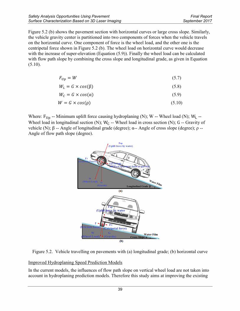
Safety Analysis Opportunities Using Pavement Final ReportSurface Characterization Based on 3D Laser Imaging September 2017
Gallaway and USF models by considering the effects of flow path slope on wheel loads as shown in Equations (511) and (512)
119907 = 09143 times 119878119863ସ times (119875௧ times 119888119900119904120588)
ଷ times (119879119863 + 0794) times 119860 (511)
119907 = (119882 times 119888119900119904120588)ଶ times (119875௧ times 119888119900119904120588)
ହ times (082 frasl119882119865119863 + 049) (512)
Where W -- Wheel load (N) WFD -- Water film depth (mm) P୲ -- Inflation pressure (Kpa) SD -- Spin down ratio TD -- Tire tread depth (mm) A -- Maximum value of Equation (4) ρ -- Angle of flow path slope (degree)
Sensitivity Analysis of the Improved Models
To explore the sensitivity of cross slope and longitudinal grade on hydroplaning speed the cross slope and longitudinal grade change by plusmn 25 plusmn 50 and plusmn 75 individually while the other variables are maintained constant values The constant values of each factor is assumed to be the average values of that factor measured for test site as provided as follows Cross slope 119878 = 153 Rainfall intensity 119868 = 1484 119898119898ℎ119903 Mean texture depth MTD = 12 mm Longitudinal grade S୪ = 132
The results of sensitivity analysis from the improved Gallaway and USF models to cross slope and longitudinal grade are given in Figure 3 It can be seen that the resulting change in hydroplaning speed VP is apparent along the increase of cross slope and longitudinal grade In the two improved models the hydroplaning speed is affected by both the vertical load and the flow path length Typically the increase in cross slope or longitudinal grade would diminish the vertical wheel load The increase in cross slope would shorten the flow path length while the increase in longitudinal grades would extend the flow path length Both the decrease in vertical load and the increase in flow path length would reduce the hydroplaning speed
Accordingly the hydroplaning speed should decrease with the increase of longitudinal slope and may either increase or decrease with the increase of cross slope depending on effects of vertical load and flow paths Figure 53 shows that hydroplaning speed goes up with the increase of the cross slope indicating the effect of flow path length on hydroplaning speed is greater than that of wheel load It is shown that hydroplaning speed is more sensitive to the cross slope than longitudinal grade in the two improved models
40
Safety Analysis Opportunities Using Pavement Final ReportSurface Characterization Based on 3D Laser Imaging September 2017
Figure 53 Sensitivity of improved hydroplaning models (a) longitudinal grade (b) cross slope
Data Preparation
Estimated Mean Texture Depth (EMTD)
The methodologies for texture measurements can be grouped into two categories static and high-speed methods The static test methods include Sand Patch Method [26] Circular Track Meter [24] and Outflow Meter [62] and their measurements are conducted on the marked or specified small areas The traditional high-speed test techniques are characterized with the laser based data acquisition systems [63] with a spot laser resulting in a single line of measurement along the longitudinal direction of pavement The measurements are continuously conducted on test sections which can be regarded as an efficient tool for network level pavement survey
The widely used texture indicators include the Mean Profile Depth (MPD) and Mean Texture Depth (MTD) [25 26] In this study the MTD methodology is applied since the estimation of water film depth is dependent on the MTD in the hydroplaning models However as the manual process to obtain MTD through the Sand Patch Method is a standard time-consuming and somewhat not reliable enough [47] the 3D pavement surface captured with the 3D Ultra technology is therefore used as an alternative to be used as input to calculate area texture simulating the Sand Patch Method The alternative substantially improves data collection efficiency and reliability of computing surface texture As a volumetric method the Estimated MTD (EMTD) is therefore introduced in the research by simulating the Sand Patch Method with 1mm 3D laser imaging data of the entire lane as shown in Equation 513 [47] EMTD and MTD are assumed to be equivalent in the presented research
ವ సಾ స ∬ [ிబி(௫௬)]ௗ௫ௗ௬ sumసభ sumసభ [ிబி(௫௬)] బ 119864119872119879119863 = (1frasl119896) times sum = (1frasl119896) times sum (513) ୀଵ ୀଵ
Where 119865(119909 119910) ndash The pixel depth at point (x y) 119863 ndash The integral or gridded area containing of MtimesN pixels 119865 ndash The maximum peak in each area D 119870 ndash The number of grids within the test sample
41
Safety Analysis Opportunities Using Pavement Final ReportSurface Characterization Based on 3D Laser Imaging September 2017
Cross Slope Calibration
A properly designed and constructed cross slope is important for safe travelling since inadequate cross slopes may result in low efficiency in drainage and steep cross slopes may lead to vehicle maneuvering difficulties Therefore the accurate measurement of cross slope is important for hydroplaning speed prediction In this study 1mm 3D pavement data and IMU data are combined together to reproduce the cross slope of pavements
IMU mounted on the vehicle can measure three Euler angles which are termed as roll (Euler angle about x-axis) pitch (Euler angle about y-axis) and yaw (Euler angle about z-axis) respectively The roll angle is to represent pavement cross slope and pitch angle is traditionally used to represent pavement longitudinal grade based on the assumption that the vehicle floor is parallel with pavement surface during travelling However in real world the vehicle floor is not parallel with pavement surface during travelling which can be caused by 1) uneven gravity distribution of the vehicle 2) vibration of the vehicle during travelling 3) pavement surface geometry and condition
This study attempts to measure the vehicles body roll angle in X coordinate (angle γ) using the collected 3D laser imaging data Two sensors mounted on the rear of the DHDV are capable of covering the entire lane The ldquotruerdquo cross slope of pavements can be approximately determined with two parameters the tilt of the vehicle floor and the slope of pavement surface captured by 3D cameras [47] As Figure 54 shows the IMU system measures the angle θ of the vehicle relative to a level datum γ is the vehicle vibration angle in X coordinate which can be calculated in Equation (514) The true cross slope can be obtained by Equation (515) However in real world the angle θ and γ are very small so the cross slope can be directly computed as the difference in slope of θ and slope of γ (Equation (516)) [64]
୷మ୷భγ = act tan ( ) (514)
α = tan(θ + γ) (515)
α = tan(θ) + tan(γ) (516)
Where α ndash Angle of cross slope (degree) γ ndash The body roll angle of vehicle (degree) θ ndash IMU roll angle (degree) L ndash The distance between left and right laser (m) yଵ ndash The vertical distance from left sensor to the pavement surface (m) yଶ ndash The vertical distance from right sensor to the pavement surface (m)
42
Safety Analysis Opportunities Using Pavement Final ReportSurface Characterization Based on 3D Laser Imaging September 2017
Figure 54 Cross slope calibration based on IMU and 1mm 3D data
Software Interface for Automated Hydroplaning Prediction
A software program named Automated Hydroplaning Prediction Program (AHPP) is developed in this study to implement data processing and analysis Figure 55 shows the main interface of AHPP Once users import the IMU and 3D image data into AHPP the two types of data (1mm 3D laser imaging data and IMU data) can be automatically matched by Distance Measurement Instrument (DMI) pulses and the calibrated cross slope can be produced by the integration of IMU data and 3D data In AHPP users can manually assign the local rainfall intensity and pavement types The AHPP outputs include EMTD WFD calibrated cross slope longitudinal grade and predicted hydroplaning speeds from various models
Figure 55 Software interface for automated hydroplaning prediction
43
Safety Analysis Opportunities Using Pavement Final ReportSurface Characterization Based on 3D Laser Imaging September 2017
Case Study
Testing Site
A flexible pavement section located in Spavinaw Oklahoma is chosen as the test section which starts from the location (Latitude 36329175 Longitude -95081696) and ends with the location (Latitude 36351066 Longitude -95062796) with a length of 435 km The pavement of the test lane is in excellent condition and has a width of 365m On this test section there are five horizontal curves
Selection of Sample Size
The 3D laser imaging data collected with the 3D Ultra DHDV is stored on computer hard disk in the form of raw data files with the size of 4096 pixel wide by 2048 pixel long The raw data files are used as basic input data sets or samples and subsequently data processing and analysis are conducted on each individual sample In this study one raw image is considered as a sample (228m long) and the entire pavement section consists of 1915 samples
Local Rainfall Intensity
The local rainfall intensity at the test site is obtained from National Oceanic and Atmospheric Administrations (NOAA) National Water Service database [65] Table 51 shows the precipitation in Spavinaw Station Oklahoma from NOAA database The two-year return period storm with duration of five minutes is used in Gallaway and USF models for rainfall intensity acquisition Based on NOAA database the rainfall intensity of 1484mmhour is used for the test site
Table 51 Precipitation in Spavinaw station Duration Recurrence Recurrence Recurrence Recurrence (in mm) - 1 year - 2 year - 5 year - 10 year 5 min 1087 1237 1491 1704
10 min 1593 1811 2182 2497 15 min 1941 2209 2667 3048 30 min 2870 3277 3962 4547
Cross Slope and Longitudinal Grade
Both longitudinal grade and cross slope are the key factors to form flow path slope As Figure 56(a) shows the maximum longitudinal grade is 1203 and the standard deviation is 248 Due to the vibration of the surveying vehicle there is some noise in the raw cross slope captured by IMU roll angle Based on the 3D laser imaging data the vehicle body roll angle can be measured and then the raw cross slope is calibrated Figure 56(b) shows the raw cross slope and calibrated cross slopes Comparing the raw cross slope data and calibrated cross slope the majority of the noise is eliminated from the raw data through the calibration The cross slope presents negative values at left turn curves and positive values at right turn curves In this test site curves 1 4 and 5 belong to left turn curve while curves 2 and 3 belong to right turn curve The statistical results of the calibrated cross slopes on test site are given as follows (1) the
44
Safety Analysis Opportunities Using Pavement Final ReportSurface Characterization Based on 3D Laser Imaging September 2017
average cross slope on the straight road segments is 194 (2) the average cross slope of curve 1 2 3 4 and 5 are -206 496 580 -381 and -501 respectively
Figure 56 Pavement geometry of the testing site (a) Longitudinal grade (b) Cross slope
EMTDs and WFDs
Figure 57(a) shows the corresponding WFD along the test section with an average value of 173mm and the maximum value of 852 mm and Figure 57(b) shows the EMTDs at the test section with an average value of 120 mm The WFD is calculated with Gallaway WFD model based on pavement texture depth flow path slope and local rainfall intensity as inputs
Figure 57 WFDs and EMTDs of test site (a) WFDs (b) EMTDS
45
Safety Analysis Opportunities Using Pavement Final ReportSurface Characterization Based on 3D Laser Imaging September 2017
Hydroplaning Speed Estimation
15 samples of the calculated WFD EMTD and IMU data for hydroplaning speed prediction are given in Table 52 Gallaway model USF model the improved Gallaway model and the improved USF model are utilized to predict hydroplaning speed respectively as shown in Figure 10(a) Results indicate the predicted hydroplaning speeds from original Gallaway and USF model are approximately 140kmh and 165kmh respectively which are around 50kmh higher than those predicted from the improved Gallaway model (96kmh) and improved USF model (91kmh) The results also show as expected that the hydroplaning speeds at curves of the five horizontal curves in Figure 58(a) are lower than that on the straight road sections
Table 52 Sample 3D and IMU data for hydroplaning speed calculation Sample ID WFD (mm) EMTD (mm) Cross Slope () Longitudinal Grade ()
1 164 112 207 327 2 151 111 226 318 3 135 111 254 310 4 130 110 268 312 5 123 111 282 307 6 121 109 287 289 7 113 112 295 278 8 105 117 305 277 9 103 114 323 272 10 100 110 344 267 11 093 112 364 271 12 094 111 374 281 13 094 110 376 285 14 086 117 379 279 15 092 110 383 276
Potential Hydroplaning Segment Detection
Identification of locations with hydroplaning potential is based on the comparison of estimated hydroplaning speed with posted speed of the road section [47] At the test site speed limits are 80kmh on straight sections and 56kmh on road curves The average hydroplaning speeds calculated with the four models are used to detect potential hydroplaning segments shown in Figure 58(a) Since the predicted hydroplaning speeds at the five curves are higher than posted speed limit there is a low hydroplaning risk at the five curves for vehicles operating at speed limit However for several segments of the test site the predicted hydroplaning speeds are lower than the posted speed limit Therefore these segments can be identified as potential segments for increased hydroplaning risk as marked with red line in Figure 58(b) To minimize traffic crashes caused by hydroplaning highway agencies can post a reduced speed sign at these locations or take other remedial actions such as installing High-Friction Surface Treatment (HFST) [66]
46
Safety Analysis Opportunities Using Pavement Final ReportSurface Characterization Based on 3D Laser Imaging September 2017
Figure 58 Detection of potential hydroplaning risk (a) hydroplaning speed (b) increased hydroplaning potential segments
47
Safety Analysis Opportunities Using Pavement Final ReportSurface Characterization Based on 3D Laser Imaging September 2017
6 SUMMARY
The 3D Ultra laser imaging technology has the capability to collect pavement surface texture data at full-lane coverage at 1 mm resolution in all three dimensions at speed up to 60MPH This single-pass and complete lane coverage platform provides an ideal solution to evaluate pavement surface characteristics for safety analysis and many different data collection needs without interrupting traffic Furthermore it will saved cost by eliminating the need for maintenance of traffic
In this study the 3D Ultra laser imaging technology with necessary software tools are utilized for data collection and subsequent surface characterization and safety evaluation and analysis First the 1mm 3D data for 21 HFST sites in 11 states with a total of 41 sections are collected for each traffic lane at the posted highway speeds Pavement rutting and macro-texture data are calculated from collected 1mm 3D data sets while pavement friction data are collected using FHWAs fixed-slip continuous friction tester The measured surface characteristics on the HFST sites and untreated existing pavements are compared and paired t-tests are performed to determine the effectiveness of the HFST sites in improving surface characteristics It is evident that the HFST surfaces have statistically significant higher friction numbers and surface macro-texture MPD values than those on the adjacent pavements without HFST There exist several exceptions to such trend 2 sections for friction data and 5 sections for MPD data Multivariate analyses are conducted to investigate the impacts of five independent variables precipitation average temperature HFST installation age aggregate type and AADT on HFST friction performance Average temperature and HFST installation age are identified to have significantly impact on friction performance of HFST (FNHFST) and the ratio of friction on HFST to that on non-HFST (FN Ratio) Based on the trend between FN Ratio and installation age in general the benefit of HFST in friction effectiveness is lost after approximate 60 months (5 years) of service HFST sites using calcined bauxite aggregates exhibit higher friction performance than those using flints The regressional friction prediction models are therefore developed for HFST which can be used to predict the service life of HFST installation and aid decision making within a highway agency However it should be noted that the models donrsquot consider the pavement conditions before HFST application and HFST construction quality variations as the dependent variables due to the unavailability of data In addition detailed traffic data for ramps and each lane of sites with multiple lanes are not available and have to be estimated during the model development
Surface texture and friction are two primary characteristics for pavement safety evaluation Understanding their relationship is critical to reduce potential traffic crashes especially at wet conditions However the currently used texture indicators such as Mean Profile Depth (MPD) and Mean Texture Depth (MTD) are calculated restricted on either a small portion on pavement surface or single line of profile measurement and thus only reveal partial aspects of texture property With 1mm 3D laser texture data eight surface texture indicators are examined for their applications on pavement friction prediction The eight surface texture indicators are grouped into four categories amplitude parameters (including MPD SMTD RMS Skewness and Kurtosis) spacing parameters (TAR) hybrid parameters (SAR) and functional parameters (SBI) To avoid using two highly correlated texture indicators in the friction prediction model correlation analyses are conducted and found that 1) SMTD are highly correlated with MPD 2)
48
Safety Analysis Opportunities Using Pavement Final ReportSurface Characterization Based on 3D Laser Imaging September 2017
RMS is highly correlated with SAR As a result six texture indicators including MPD Skewness Kurtosis TAR SAR and SBI are adopted for the development of pavement friction prediction model using multivariate regression analysis The developed model can be used to predict pavement friction based on various texture indicators and may be beneficial in the continuous measurement and evaluation of pavement safety for the project- and network- level pavement surveys
The third application of using 1mm 3D Ultra data sets is to predict and evaluate pavement surface hydroplaning risk Considering the effects of flow path slope on vertical wheel load perpendicular to pavement surface and the resulting hydroplaning speed the Gallaway and USF models are modified for improvements in this study The sensitivity analysis shows that the hydroplaning speed is more sensitive to cross slope than longitudinal grade in the improved models A 3D based volumetric measuring method is used to calculate the estimated MTD based on the full-lane 1mm 3D data Subsequently IMU data and 3D data are combined to model vehicle movements on cross slopes Local rainfall intensity is obtained from NOAA precipitation database By considering effects of cross slope and longitudinal grade on wheel load and flow path length it is found that hydroplaning speed decreases with the increase of the longitudinal grade but increases with the increase of the cross slope The improved models predict lower hydroplaning speed than that from the original Gallaway and USF models An important future work is to use a combined slope based on longitudinal grade and cross slope to demonstrate the validity and effectiveness of the improved models
This study with field pavement applications has shown that the 1mm 3D Ultra which represent a form of 3D Laser imaging technology is promising in real-time pavement surface characterization and evaluation for both pavement and safety management at network and project level surveys It is anticipated that more data collection with more testing sites are to be performed to validate the new emerging 3D laser imaging technology as a single-pass and complete lane-coverage platform for multiple safety and pavement evaluation purposes In addition the long-term monitoring of the HFTS sites in multiple states is highly recommended due to the need to determine multi-year performance of the HFTS applications in terms of region pavement condition materials used geometric properties and other factors The recommended long-term study would provide much needed data for both design and construction of HFTS for its widespread adoption
49
Safety Analysis Opportunities Using Pavement Final ReportSurface Characterization Based on 3D Laser Imaging September 2017
REFERENCES
[1] Brimley B and Carlson P Using High Friction Surface Treatments to Improve Safety at Horizontal Curves Texas Transportation Institute httpd2dtl5nnlpfr0rcloudfrontnetttitamuedudocumentsTTI-2012-8pdf 2012 (accessed 150625)
[2] The Trans Tec Group INC Welcome to High Friction Roads httpwwwhighfrictionroadscom 2015 (accessed 150725)
[3] Bledsoe J Missouri Demonstration Project The Use of High-Friction Surface Treatments on Missouri Highways FHWA US Department of Transportation httpplan4operationsdotgovhflsummarypdf_2Missouri20High20Friction20Report 20draft20Finalpdf 2015 (accessed 150630)
[4] Moravec M High Friction Surface Treatments at High-Crash Horizontal Curves Arizona PavementsMaterials Conference Phoenix AZ httpwwwintransiastateedueventsmidcon2013documentspresentation-submissions3-C_61_08142013pdf 2013 (accessed 150630)
[5] South Dakota Department of Transportation (SDDOT) Accelerated Innovation Deployment (AID) Demonstration Project High Friction Surface Treatment httpwwwfhwadotgovacceleratinggrantspdfsSD_2014_AID_Grantpdf 2015 (accessed 150611)
[6] Bischoff D Investigative Study of the Italgrip TM System WI-04-08 Wisconsin Department of Transportation Madison WI httpwisdotresearchwigovwp-contentuploadswi-04-08italgrippdf 2008 (accessed 150620)
[7] Izeppi E Flintsch G and McGhee K Field Performance of High Friction Surfaces Publication FHWAVTRC 10-CR6 FHWA US Department of Transportation httpwwwvirginiadotorgvtrcmainonline_reportspdf10-cr6pdf 2010 (accessed 150615)
[8] Waters J High Friction Surfacing Failure Mechanisms 3rd International Surface Friction Conference Safer Road Surfaces ndash Saving Lives Gold Coast Australia 2011
[9] Wang Kelvin C P Elements of Automated Survey of Pavements and a 3D Methodology J mod transp Vol 19 pp 51-57 2011
[10] AASTHO Quantifying cracks in asphalt pavement surfaces from collected images utilizing automated methods AASHTO Designation PP67-10 American Association of State Highway and Transportation Officials Washington DC 2013
[11] AASTHO 2013 Standard Practice for Determining Pavement Deformation Parameters and Cross Slope from Collected Transverse Profiles AASHTO Designation PP69-10 American Association of State Highway and Transportation Officials Washington DC 2013
[12] Hall J W Smith K L Titus-Glover L Wambold J C Yager T J and Rado Z Guide for Pavement Friction Final Report for NCHRP Project 01-43 National Cooperative
50
Safety Analysis Opportunities Using Pavement Final ReportSurface Characterization Based on 3D Laser Imaging September 2017
Highway Research Program (NCHRP) Transportation Research Board (TRB) Washington DC 2009
[13] Ahammed MA and Tighe SL Concrete Pavement Surface Textures and Multivariables Frictional Performance Analysis a North American Case Study Can J Civil Eng Vol 35 727-738 2008
[14] Ergun M Iyinam S and Iyinam AF Prediction of Road Surface Friction Coefficient Using Only Macro- and Microtexture Measurements J Transp Eng Vol 131 pp 311-319 2005
[15] Flintsch GW et al The Little Book of Tire Pavement Friction Pavement Surface Properties Consortium httpssecurehostingvteduwwwappsvttivtedu1-pagersCSTI_FlintschThe20Little20Book20of20Tire20Pavement20Frictionpdf 2012 (accessed 150501)
[16] Henry J J NCHRP Synthesis 291 Evaluation of Pavement Friction Characteristics TRB National Research Council Washington DC 2000
[17] Ahammed MA and Tighe SL Effect of Short-term and Long-term Weather on Pavement Surface Friction Int J Na Res Tech Vol 3 pp 295-302 2010
[18] Luo Y Effect of Pavement Temperature on Frictional Properties of Hot-Mix-Asphalt Pavement Surfaces at the Virginia Smart Road MS Thesis Virginia Polytechnic Institute and State University Blacksburg Va 2003
[19] Fuents L G Investigation of the Factors Influencing Skid Resistance and the International Friction Index PhD Thesis University of South Florida Tampa FL 2009
[20] American Society for Testing and Materials (ASTM) ASTM E 867 Standard Terminology Relating to Vehicle-Pavement Systems ASTM Standard Practice E 867 Book of ASTM Standards Volume 0403 Philadelphia P A 2011
[21] International Standards Organization (ISO) Characterization of Pavement Texture using Surface Profiles ndash Part 1 Determination of Mean Profile Depth Acoustics ISO Standard 13473 International Standards Organization Geneva Switzerland 1998
[22] PIARC World Road Association Report of the Committee on Surface Characteristics In Proceeding of XVIII World Road Congress Brussels Belgium pp 13ndash19 1987
[23] Sandburg U Influence of Road Surface Texture on Traffic Characteristics Related to Environment Economy and Safety A State-of-the-Art Study Regarding Measures and Measuring Methods VTI Report 53A-1997 Swedish National Road Administration Borlange Sweden 1998
[24] American Society for Testing and Materials (ASTM) ASTM E 2157 Standard Test Method for Measuring Pavement Macro texture Properties Using the Circular Track Meter ASTM Standard Practice E 2157 Book of ASTM Standards Volume 0403 Philadelphia P A 2011
51
Safety Analysis Opportunities Using Pavement Final ReportSurface Characterization Based on 3D Laser Imaging September 2017
[25] American Society for Testing and Materials (ASTM) ASTM E 1845 Calculating Pavement Macro texture Profile Depth ASTM Standard Practice E 1845 Book of ASTM Standards Volume 0403 Philadelphia P A 2011
[26] American Society for Testing and Materials (ASTM) ASTM E 965 Standard Test Method for Measuring Pavement Macro texture Depth Using a Volumetric Technique ASTM Standard Practice E 965 Book of ASTM Standards Volume 0403 Philadelphia P A 2011
[27] McGhee K K amp Flintsch G W High-speed Texture Measurement of Pavements Virginia Transportation Research Council Charlottesville VA 2003
[28] Prowell B amp Hanson D Evaluation of Circular Texture Meter for Measuring Surface Texture of Pavements Transportation Research Record Journal of the Transportation Research Board No 1929 pp 88-96 2005
[29] Alvarez L amp Morel J M Formalization and Computational Aspects of Image Analysis Acta numerica Vol 3 pp 1-59 1994
[30] Gendy A E amp Shalaby A Mean Profile Depth of Pavement Surface Macrotexture Using Photometric Stereo Techniques Journal of Transportation Engineering Vol 133 No 7 pp 433-440 2007
[31] Kokkalis A and Panagouli O Fractal Evaluation of Pavement Skid Resistance Variations I Surface Wetting Chaos Solitons amp Fractals pp 1875-1890 1998
[32] American Society for Testing and Materials (ASTM) ASTM E 274 Standard Test Method for Skid Resistance of Paved Surfaces Using a Full-Scale Tire ASTM Standard Practice E 274 Book of ASTM Standards Volume 0403 Philadelphia P A 2011
[33] American Society for Testing and Materials (ASTM) ASTM E 303 Standard Test Method for Measuring Surface Frictional Properties Using a British Pendulum Tester ASTM Standard Practice E 303 Book of ASTM Standards Volume 0403 Philadelphia P A 2011
[34] Janoo VC and Horhonen C Performance Testing of Hot-Mix Asphalt Aggregates Special Report pp 99-20 1999
[35] Kuennen T Creating Friction Where Rubber Meets the Road Better Roads Vol 73 No 10 2003
[36] Leu MC Henry JJ Prediction of skid resistance as a function of speed from pavement texture measurements Transportation Research Record No 666 pp 7-13 1978
[37] Yager T J and Buhlmann F Macrotexture and Drainage Measurements on a Variety of Concrete and Asphalt Surfaces Pavement Surface Characteristics and Materials ASTM STP 763 pp 16-30 1982
[38] Rado Z Analysis of Texture Models PTI Report No 9510 Pennsylvania Transportation Institute (PTI) Penn State University State College Pennsylvania 1994
52
Safety Analysis Opportunities Using Pavement Final ReportSurface Characterization Based on 3D Laser Imaging September 2017
[39] Fwa T F Choo Y S and Liu Y (2003) Effect of Aggregate Spacing on Skid Resistance of Asphalt Pavement Journal of Transportation Engineering Vol 129 No 4 pp 420-426 2003
[40] Olek J Weiss W J and Garcia-Villarreal R Relating Surface Texture of Rigid Pavement with Noise and Skid Resistance Purdue University West Lafayette Indiana Report No SQDH-2004-1 (Final Report HL 2004-1) 2004
[41] Do MT Marsac P Delanne Y Prediction of Tirewet Road Friction from Road Surface Microtexture and Tire Rubber Properties In 5th International Symposium on Pavement Surface Characteristics Toronto 2004
[42] Ergun M Iyinam S amp Iyinam A F (2005) Prediction of Road Surface Friction Coefficient Using only Macro- and Micro texture Measurement Journal of transportation engineering Vol 131 No 4 pp 311-319 2005
[43] Kebrle J Walker R Texture measurement and friction estimation using laser data acquisition and neural networks In Proceedings of the 9th WSEAS International Conference on Mathematical and Computational Methods in Science and Engineering Trinidad and Tobago 2007
[44] Rezaei A Masad E Chowdhury A amp Harris P Predicting Asphalt Mixture Skid Resistance by Aggregate Characteristics and Gradation Transportation Research Record Journal of the Transportation Research Board No 2014 pp 24-33 2009
[45] American National Standards Institute Surface texture surface roughness waviness and lay American Society of Mechanical Engineers 1986
[46] Stout K J Sullivan PJ Dong WP Mainsah E Luo N Mathia T and Zahyouani H The development of methods for the characterization of roughness in three dimensions Commission of the European Communities 1993
[47] Luo Wenting Wang Kelvin C P Li Lin 2014 Surface Drainage Evaluation for Rigid Pavements Using IMU and 1 mm 3D Texture Data Transportation Research Record Journal of the Transportation Research Board Washington DC Pavement Management 2014 Volume 3 pp 121ndash128 2014
[48] Tsai C L Cai Z amp Wu X (1998) The examination of residual plots Statistica Sinica Vol 8 pp 445-465 1998
[49] Kumar SSantosh Anupam Kumar and FWA TF Analyzing effect of tire groove patterns on hydroplaning speed Journal of the Eastern Asia Society for Transportation Studies Vol 8 2009
[50] Khedr Safwan A and Breakah Tamer M Rutting parameters for asphalt concrete for different aggregate structures International Journal of Pavement Engineering Volume 12 Issue 1 pp 13-23 2011
53
Safety Analysis Opportunities Using Pavement Final ReportSurface Characterization Based on 3D Laser Imaging September 2017
[51] MISH Rohit Goyal Design and Analysis of Interceptor DrainsmdashEffect of Parameters ISH Journal of Hydraulic Engineering Volume 9 Issue 1 pp 61-71 2003
[52] Horne WB and RC Dreher Phenomena of Pneumatic Tire Hydroplaning NASA TN D-2-56 NASA Langley Research center NASA Hampton VA 1963
[53] Chesterton John Nancekivell Noel and Tunnicliffe Noel The use of the Gallaway Formula for Aquaplaning Evaluation in New Zealand Transit New Zealand and New Zealand Institute of Highway Technology (NZIHT) 8thAnnual Conference 2006
[54] Russam K and Ross NF The Depth of Rain Water on Road Surfaces Road Research Laboratory Ministry of Transport Report No LR 236 pp25 1968
[55] Gallaway B M et al Pavement and Geometric Design Criteria for Minimizing Hydroplaning Federal Highway Administration Report No FHWA-RD-79-31 1979
[56] Huebner RS et al PAVDRN Computer Model for Predicting Water Film Thickness and Potential or Hydroplaning on New and Reconditioned Pavements Transport Research Record 1599 pp 128-131 1996
[57] Gunaratne M Lu Q Yang J Hydroplaning on Multi Lane Facilities Report for Florida Department of Transportation Report No BDK84 977-14 2012
[58] Zhang Zhongjie Abu-Farsakh Murad Y and Tao Mingjiang Evaluation of trench backfills at highway cross-drains International Journal of Pavement Engineering Volume 6 Issue 2 pp77-87 2005
[59] Gallaway B M and Rose Gerry The Effects of Rainfall Intensity Pavement Cross Slope Surface Texture and Drainage Length on Pavement Water Depths Texas Transportation Institute Research Report No 138-5 1971
[60] Ong GP and Fwa TF Wet-pavement hydroplaning risk and skid-resistance Modeling ASCE Journal of Transportation Engineering Vol 133 No 10 2007
[61] Shafabakhsh GA Kashi E Effect of Aircraft Wheel Load and Configuration on Runway Damages Period Polytech Civil Eng Vol 59 No 1 pp 85-94 2015
[62] ASTM Measuring Pavement Texture Drainage Using an Outflow ASTM Standard Practice E 2380 Book of ASTM Standards Volume 0403 Philadelphia P A 2006
[63] ASTM Measuring Surface Frictional Properties Using the British Pendulum Tester ASTM Standard Practice E 303 Book of ASTM Standards Volume 0403 Philadelphia P A 2006
[64] Mekemson et al Method and Apparatus for Pavement Cross-slope Measurement Patent Application Publication Pub No US 20020013644 A1 2002
54
Safety Analysis Opportunities Using Pavement Final ReportSurface Characterization Based on 3D Laser Imaging September 2017
[65] NOAAs National Water Service Hydrometeorological Design Studies Center Precipitation Frequency Data Server (PFDS) httpdippernwsnoaagovhdscpfds Accessed on July 2014
[66] Shah Yogesh U Jain SS and Parida Manoranjan Evaluation of prioritization methods for effective pavement maintenance of urban roads International Journal of Pavement Engineering Volume 15 Issue 3 pp 238-250 2014
55
For More Information
Safety Analysis Opportunities Using Pavement Surface Characterization
Based on 3D Laser Imaging visit httpsafetyfhwadotgov
July 2017 FHWA-SA-17-046
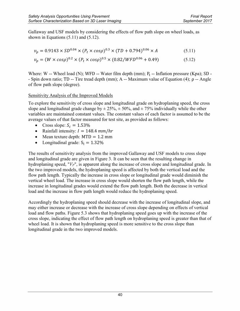
Safety Analysis Opportunities Using Pavement Final ReportSurface Characterization Based on 3D Laser Imaging September 2017
Figure 53 Sensitivity of improved hydroplaning models (a) longitudinal grade (b) cross slope
Data Preparation
Estimated Mean Texture Depth (EMTD)
The methodologies for texture measurements can be grouped into two categories static and high-speed methods The static test methods include Sand Patch Method [26] Circular Track Meter [24] and Outflow Meter [62] and their measurements are conducted on the marked or specified small areas The traditional high-speed test techniques are characterized with the laser based data acquisition systems [63] with a spot laser resulting in a single line of measurement along the longitudinal direction of pavement The measurements are continuously conducted on test sections which can be regarded as an efficient tool for network level pavement survey
The widely used texture indicators include the Mean Profile Depth (MPD) and Mean Texture Depth (MTD) [25 26] In this study the MTD methodology is applied since the estimation of water film depth is dependent on the MTD in the hydroplaning models However as the manual process to obtain MTD through the Sand Patch Method is a standard time-consuming and somewhat not reliable enough [47] the 3D pavement surface captured with the 3D Ultra technology is therefore used as an alternative to be used as input to calculate area texture simulating the Sand Patch Method The alternative substantially improves data collection efficiency and reliability of computing surface texture As a volumetric method the Estimated MTD (EMTD) is therefore introduced in the research by simulating the Sand Patch Method with 1mm 3D laser imaging data of the entire lane as shown in Equation 513 [47] EMTD and MTD are assumed to be equivalent in the presented research
ವ సಾ స ∬ [ிబி(௫௬)]ௗ௫ௗ௬ sumసభ sumసభ [ிబி(௫௬)] బ 119864119872119879119863 = (1frasl119896) times sum = (1frasl119896) times sum (513) ୀଵ ୀଵ
Where 119865(119909 119910) ndash The pixel depth at point (x y) 119863 ndash The integral or gridded area containing of MtimesN pixels 119865 ndash The maximum peak in each area D 119870 ndash The number of grids within the test sample
41
Safety Analysis Opportunities Using Pavement Final ReportSurface Characterization Based on 3D Laser Imaging September 2017
Cross Slope Calibration
A properly designed and constructed cross slope is important for safe travelling since inadequate cross slopes may result in low efficiency in drainage and steep cross slopes may lead to vehicle maneuvering difficulties Therefore the accurate measurement of cross slope is important for hydroplaning speed prediction In this study 1mm 3D pavement data and IMU data are combined together to reproduce the cross slope of pavements
IMU mounted on the vehicle can measure three Euler angles which are termed as roll (Euler angle about x-axis) pitch (Euler angle about y-axis) and yaw (Euler angle about z-axis) respectively The roll angle is to represent pavement cross slope and pitch angle is traditionally used to represent pavement longitudinal grade based on the assumption that the vehicle floor is parallel with pavement surface during travelling However in real world the vehicle floor is not parallel with pavement surface during travelling which can be caused by 1) uneven gravity distribution of the vehicle 2) vibration of the vehicle during travelling 3) pavement surface geometry and condition
This study attempts to measure the vehicles body roll angle in X coordinate (angle γ) using the collected 3D laser imaging data Two sensors mounted on the rear of the DHDV are capable of covering the entire lane The ldquotruerdquo cross slope of pavements can be approximately determined with two parameters the tilt of the vehicle floor and the slope of pavement surface captured by 3D cameras [47] As Figure 54 shows the IMU system measures the angle θ of the vehicle relative to a level datum γ is the vehicle vibration angle in X coordinate which can be calculated in Equation (514) The true cross slope can be obtained by Equation (515) However in real world the angle θ and γ are very small so the cross slope can be directly computed as the difference in slope of θ and slope of γ (Equation (516)) [64]
୷మ୷భγ = act tan ( ) (514)
α = tan(θ + γ) (515)
α = tan(θ) + tan(γ) (516)
Where α ndash Angle of cross slope (degree) γ ndash The body roll angle of vehicle (degree) θ ndash IMU roll angle (degree) L ndash The distance between left and right laser (m) yଵ ndash The vertical distance from left sensor to the pavement surface (m) yଶ ndash The vertical distance from right sensor to the pavement surface (m)
42
Safety Analysis Opportunities Using Pavement Final ReportSurface Characterization Based on 3D Laser Imaging September 2017
Figure 54 Cross slope calibration based on IMU and 1mm 3D data
Software Interface for Automated Hydroplaning Prediction
A software program named Automated Hydroplaning Prediction Program (AHPP) is developed in this study to implement data processing and analysis Figure 55 shows the main interface of AHPP Once users import the IMU and 3D image data into AHPP the two types of data (1mm 3D laser imaging data and IMU data) can be automatically matched by Distance Measurement Instrument (DMI) pulses and the calibrated cross slope can be produced by the integration of IMU data and 3D data In AHPP users can manually assign the local rainfall intensity and pavement types The AHPP outputs include EMTD WFD calibrated cross slope longitudinal grade and predicted hydroplaning speeds from various models
Figure 55 Software interface for automated hydroplaning prediction
43
Safety Analysis Opportunities Using Pavement Final ReportSurface Characterization Based on 3D Laser Imaging September 2017
Case Study
Testing Site
A flexible pavement section located in Spavinaw Oklahoma is chosen as the test section which starts from the location (Latitude 36329175 Longitude -95081696) and ends with the location (Latitude 36351066 Longitude -95062796) with a length of 435 km The pavement of the test lane is in excellent condition and has a width of 365m On this test section there are five horizontal curves
Selection of Sample Size
The 3D laser imaging data collected with the 3D Ultra DHDV is stored on computer hard disk in the form of raw data files with the size of 4096 pixel wide by 2048 pixel long The raw data files are used as basic input data sets or samples and subsequently data processing and analysis are conducted on each individual sample In this study one raw image is considered as a sample (228m long) and the entire pavement section consists of 1915 samples
Local Rainfall Intensity
The local rainfall intensity at the test site is obtained from National Oceanic and Atmospheric Administrations (NOAA) National Water Service database [65] Table 51 shows the precipitation in Spavinaw Station Oklahoma from NOAA database The two-year return period storm with duration of five minutes is used in Gallaway and USF models for rainfall intensity acquisition Based on NOAA database the rainfall intensity of 1484mmhour is used for the test site
Table 51 Precipitation in Spavinaw station Duration Recurrence Recurrence Recurrence Recurrence (in mm) - 1 year - 2 year - 5 year - 10 year 5 min 1087 1237 1491 1704
10 min 1593 1811 2182 2497 15 min 1941 2209 2667 3048 30 min 2870 3277 3962 4547
Cross Slope and Longitudinal Grade
Both longitudinal grade and cross slope are the key factors to form flow path slope As Figure 56(a) shows the maximum longitudinal grade is 1203 and the standard deviation is 248 Due to the vibration of the surveying vehicle there is some noise in the raw cross slope captured by IMU roll angle Based on the 3D laser imaging data the vehicle body roll angle can be measured and then the raw cross slope is calibrated Figure 56(b) shows the raw cross slope and calibrated cross slopes Comparing the raw cross slope data and calibrated cross slope the majority of the noise is eliminated from the raw data through the calibration The cross slope presents negative values at left turn curves and positive values at right turn curves In this test site curves 1 4 and 5 belong to left turn curve while curves 2 and 3 belong to right turn curve The statistical results of the calibrated cross slopes on test site are given as follows (1) the
44
Safety Analysis Opportunities Using Pavement Final ReportSurface Characterization Based on 3D Laser Imaging September 2017
average cross slope on the straight road segments is 194 (2) the average cross slope of curve 1 2 3 4 and 5 are -206 496 580 -381 and -501 respectively
Figure 56 Pavement geometry of the testing site (a) Longitudinal grade (b) Cross slope
EMTDs and WFDs
Figure 57(a) shows the corresponding WFD along the test section with an average value of 173mm and the maximum value of 852 mm and Figure 57(b) shows the EMTDs at the test section with an average value of 120 mm The WFD is calculated with Gallaway WFD model based on pavement texture depth flow path slope and local rainfall intensity as inputs
Figure 57 WFDs and EMTDs of test site (a) WFDs (b) EMTDS
45
Safety Analysis Opportunities Using Pavement Final ReportSurface Characterization Based on 3D Laser Imaging September 2017
Hydroplaning Speed Estimation
15 samples of the calculated WFD EMTD and IMU data for hydroplaning speed prediction are given in Table 52 Gallaway model USF model the improved Gallaway model and the improved USF model are utilized to predict hydroplaning speed respectively as shown in Figure 10(a) Results indicate the predicted hydroplaning speeds from original Gallaway and USF model are approximately 140kmh and 165kmh respectively which are around 50kmh higher than those predicted from the improved Gallaway model (96kmh) and improved USF model (91kmh) The results also show as expected that the hydroplaning speeds at curves of the five horizontal curves in Figure 58(a) are lower than that on the straight road sections
Table 52 Sample 3D and IMU data for hydroplaning speed calculation Sample ID WFD (mm) EMTD (mm) Cross Slope () Longitudinal Grade ()
1 164 112 207 327 2 151 111 226 318 3 135 111 254 310 4 130 110 268 312 5 123 111 282 307 6 121 109 287 289 7 113 112 295 278 8 105 117 305 277 9 103 114 323 272 10 100 110 344 267 11 093 112 364 271 12 094 111 374 281 13 094 110 376 285 14 086 117 379 279 15 092 110 383 276
Potential Hydroplaning Segment Detection
Identification of locations with hydroplaning potential is based on the comparison of estimated hydroplaning speed with posted speed of the road section [47] At the test site speed limits are 80kmh on straight sections and 56kmh on road curves The average hydroplaning speeds calculated with the four models are used to detect potential hydroplaning segments shown in Figure 58(a) Since the predicted hydroplaning speeds at the five curves are higher than posted speed limit there is a low hydroplaning risk at the five curves for vehicles operating at speed limit However for several segments of the test site the predicted hydroplaning speeds are lower than the posted speed limit Therefore these segments can be identified as potential segments for increased hydroplaning risk as marked with red line in Figure 58(b) To minimize traffic crashes caused by hydroplaning highway agencies can post a reduced speed sign at these locations or take other remedial actions such as installing High-Friction Surface Treatment (HFST) [66]
46
Safety Analysis Opportunities Using Pavement Final ReportSurface Characterization Based on 3D Laser Imaging September 2017
Figure 58 Detection of potential hydroplaning risk (a) hydroplaning speed (b) increased hydroplaning potential segments
47
Safety Analysis Opportunities Using Pavement Final ReportSurface Characterization Based on 3D Laser Imaging September 2017
6 SUMMARY
The 3D Ultra laser imaging technology has the capability to collect pavement surface texture data at full-lane coverage at 1 mm resolution in all three dimensions at speed up to 60MPH This single-pass and complete lane coverage platform provides an ideal solution to evaluate pavement surface characteristics for safety analysis and many different data collection needs without interrupting traffic Furthermore it will saved cost by eliminating the need for maintenance of traffic
In this study the 3D Ultra laser imaging technology with necessary software tools are utilized for data collection and subsequent surface characterization and safety evaluation and analysis First the 1mm 3D data for 21 HFST sites in 11 states with a total of 41 sections are collected for each traffic lane at the posted highway speeds Pavement rutting and macro-texture data are calculated from collected 1mm 3D data sets while pavement friction data are collected using FHWAs fixed-slip continuous friction tester The measured surface characteristics on the HFST sites and untreated existing pavements are compared and paired t-tests are performed to determine the effectiveness of the HFST sites in improving surface characteristics It is evident that the HFST surfaces have statistically significant higher friction numbers and surface macro-texture MPD values than those on the adjacent pavements without HFST There exist several exceptions to such trend 2 sections for friction data and 5 sections for MPD data Multivariate analyses are conducted to investigate the impacts of five independent variables precipitation average temperature HFST installation age aggregate type and AADT on HFST friction performance Average temperature and HFST installation age are identified to have significantly impact on friction performance of HFST (FNHFST) and the ratio of friction on HFST to that on non-HFST (FN Ratio) Based on the trend between FN Ratio and installation age in general the benefit of HFST in friction effectiveness is lost after approximate 60 months (5 years) of service HFST sites using calcined bauxite aggregates exhibit higher friction performance than those using flints The regressional friction prediction models are therefore developed for HFST which can be used to predict the service life of HFST installation and aid decision making within a highway agency However it should be noted that the models donrsquot consider the pavement conditions before HFST application and HFST construction quality variations as the dependent variables due to the unavailability of data In addition detailed traffic data for ramps and each lane of sites with multiple lanes are not available and have to be estimated during the model development
Surface texture and friction are two primary characteristics for pavement safety evaluation Understanding their relationship is critical to reduce potential traffic crashes especially at wet conditions However the currently used texture indicators such as Mean Profile Depth (MPD) and Mean Texture Depth (MTD) are calculated restricted on either a small portion on pavement surface or single line of profile measurement and thus only reveal partial aspects of texture property With 1mm 3D laser texture data eight surface texture indicators are examined for their applications on pavement friction prediction The eight surface texture indicators are grouped into four categories amplitude parameters (including MPD SMTD RMS Skewness and Kurtosis) spacing parameters (TAR) hybrid parameters (SAR) and functional parameters (SBI) To avoid using two highly correlated texture indicators in the friction prediction model correlation analyses are conducted and found that 1) SMTD are highly correlated with MPD 2)
48
Safety Analysis Opportunities Using Pavement Final ReportSurface Characterization Based on 3D Laser Imaging September 2017
RMS is highly correlated with SAR As a result six texture indicators including MPD Skewness Kurtosis TAR SAR and SBI are adopted for the development of pavement friction prediction model using multivariate regression analysis The developed model can be used to predict pavement friction based on various texture indicators and may be beneficial in the continuous measurement and evaluation of pavement safety for the project- and network- level pavement surveys
The third application of using 1mm 3D Ultra data sets is to predict and evaluate pavement surface hydroplaning risk Considering the effects of flow path slope on vertical wheel load perpendicular to pavement surface and the resulting hydroplaning speed the Gallaway and USF models are modified for improvements in this study The sensitivity analysis shows that the hydroplaning speed is more sensitive to cross slope than longitudinal grade in the improved models A 3D based volumetric measuring method is used to calculate the estimated MTD based on the full-lane 1mm 3D data Subsequently IMU data and 3D data are combined to model vehicle movements on cross slopes Local rainfall intensity is obtained from NOAA precipitation database By considering effects of cross slope and longitudinal grade on wheel load and flow path length it is found that hydroplaning speed decreases with the increase of the longitudinal grade but increases with the increase of the cross slope The improved models predict lower hydroplaning speed than that from the original Gallaway and USF models An important future work is to use a combined slope based on longitudinal grade and cross slope to demonstrate the validity and effectiveness of the improved models
This study with field pavement applications has shown that the 1mm 3D Ultra which represent a form of 3D Laser imaging technology is promising in real-time pavement surface characterization and evaluation for both pavement and safety management at network and project level surveys It is anticipated that more data collection with more testing sites are to be performed to validate the new emerging 3D laser imaging technology as a single-pass and complete lane-coverage platform for multiple safety and pavement evaluation purposes In addition the long-term monitoring of the HFTS sites in multiple states is highly recommended due to the need to determine multi-year performance of the HFTS applications in terms of region pavement condition materials used geometric properties and other factors The recommended long-term study would provide much needed data for both design and construction of HFTS for its widespread adoption
49
Safety Analysis Opportunities Using Pavement Final ReportSurface Characterization Based on 3D Laser Imaging September 2017
REFERENCES
[1] Brimley B and Carlson P Using High Friction Surface Treatments to Improve Safety at Horizontal Curves Texas Transportation Institute httpd2dtl5nnlpfr0rcloudfrontnetttitamuedudocumentsTTI-2012-8pdf 2012 (accessed 150625)
[2] The Trans Tec Group INC Welcome to High Friction Roads httpwwwhighfrictionroadscom 2015 (accessed 150725)
[3] Bledsoe J Missouri Demonstration Project The Use of High-Friction Surface Treatments on Missouri Highways FHWA US Department of Transportation httpplan4operationsdotgovhflsummarypdf_2Missouri20High20Friction20Report 20draft20Finalpdf 2015 (accessed 150630)
[4] Moravec M High Friction Surface Treatments at High-Crash Horizontal Curves Arizona PavementsMaterials Conference Phoenix AZ httpwwwintransiastateedueventsmidcon2013documentspresentation-submissions3-C_61_08142013pdf 2013 (accessed 150630)
[5] South Dakota Department of Transportation (SDDOT) Accelerated Innovation Deployment (AID) Demonstration Project High Friction Surface Treatment httpwwwfhwadotgovacceleratinggrantspdfsSD_2014_AID_Grantpdf 2015 (accessed 150611)
[6] Bischoff D Investigative Study of the Italgrip TM System WI-04-08 Wisconsin Department of Transportation Madison WI httpwisdotresearchwigovwp-contentuploadswi-04-08italgrippdf 2008 (accessed 150620)
[7] Izeppi E Flintsch G and McGhee K Field Performance of High Friction Surfaces Publication FHWAVTRC 10-CR6 FHWA US Department of Transportation httpwwwvirginiadotorgvtrcmainonline_reportspdf10-cr6pdf 2010 (accessed 150615)
[8] Waters J High Friction Surfacing Failure Mechanisms 3rd International Surface Friction Conference Safer Road Surfaces ndash Saving Lives Gold Coast Australia 2011
[9] Wang Kelvin C P Elements of Automated Survey of Pavements and a 3D Methodology J mod transp Vol 19 pp 51-57 2011
[10] AASTHO Quantifying cracks in asphalt pavement surfaces from collected images utilizing automated methods AASHTO Designation PP67-10 American Association of State Highway and Transportation Officials Washington DC 2013
[11] AASTHO 2013 Standard Practice for Determining Pavement Deformation Parameters and Cross Slope from Collected Transverse Profiles AASHTO Designation PP69-10 American Association of State Highway and Transportation Officials Washington DC 2013
[12] Hall J W Smith K L Titus-Glover L Wambold J C Yager T J and Rado Z Guide for Pavement Friction Final Report for NCHRP Project 01-43 National Cooperative
50
Safety Analysis Opportunities Using Pavement Final ReportSurface Characterization Based on 3D Laser Imaging September 2017
Highway Research Program (NCHRP) Transportation Research Board (TRB) Washington DC 2009
[13] Ahammed MA and Tighe SL Concrete Pavement Surface Textures and Multivariables Frictional Performance Analysis a North American Case Study Can J Civil Eng Vol 35 727-738 2008
[14] Ergun M Iyinam S and Iyinam AF Prediction of Road Surface Friction Coefficient Using Only Macro- and Microtexture Measurements J Transp Eng Vol 131 pp 311-319 2005
[15] Flintsch GW et al The Little Book of Tire Pavement Friction Pavement Surface Properties Consortium httpssecurehostingvteduwwwappsvttivtedu1-pagersCSTI_FlintschThe20Little20Book20of20Tire20Pavement20Frictionpdf 2012 (accessed 150501)
[16] Henry J J NCHRP Synthesis 291 Evaluation of Pavement Friction Characteristics TRB National Research Council Washington DC 2000
[17] Ahammed MA and Tighe SL Effect of Short-term and Long-term Weather on Pavement Surface Friction Int J Na Res Tech Vol 3 pp 295-302 2010
[18] Luo Y Effect of Pavement Temperature on Frictional Properties of Hot-Mix-Asphalt Pavement Surfaces at the Virginia Smart Road MS Thesis Virginia Polytechnic Institute and State University Blacksburg Va 2003
[19] Fuents L G Investigation of the Factors Influencing Skid Resistance and the International Friction Index PhD Thesis University of South Florida Tampa FL 2009
[20] American Society for Testing and Materials (ASTM) ASTM E 867 Standard Terminology Relating to Vehicle-Pavement Systems ASTM Standard Practice E 867 Book of ASTM Standards Volume 0403 Philadelphia P A 2011
[21] International Standards Organization (ISO) Characterization of Pavement Texture using Surface Profiles ndash Part 1 Determination of Mean Profile Depth Acoustics ISO Standard 13473 International Standards Organization Geneva Switzerland 1998
[22] PIARC World Road Association Report of the Committee on Surface Characteristics In Proceeding of XVIII World Road Congress Brussels Belgium pp 13ndash19 1987
[23] Sandburg U Influence of Road Surface Texture on Traffic Characteristics Related to Environment Economy and Safety A State-of-the-Art Study Regarding Measures and Measuring Methods VTI Report 53A-1997 Swedish National Road Administration Borlange Sweden 1998
[24] American Society for Testing and Materials (ASTM) ASTM E 2157 Standard Test Method for Measuring Pavement Macro texture Properties Using the Circular Track Meter ASTM Standard Practice E 2157 Book of ASTM Standards Volume 0403 Philadelphia P A 2011
51
Safety Analysis Opportunities Using Pavement Final ReportSurface Characterization Based on 3D Laser Imaging September 2017
[25] American Society for Testing and Materials (ASTM) ASTM E 1845 Calculating Pavement Macro texture Profile Depth ASTM Standard Practice E 1845 Book of ASTM Standards Volume 0403 Philadelphia P A 2011
[26] American Society for Testing and Materials (ASTM) ASTM E 965 Standard Test Method for Measuring Pavement Macro texture Depth Using a Volumetric Technique ASTM Standard Practice E 965 Book of ASTM Standards Volume 0403 Philadelphia P A 2011
[27] McGhee K K amp Flintsch G W High-speed Texture Measurement of Pavements Virginia Transportation Research Council Charlottesville VA 2003
[28] Prowell B amp Hanson D Evaluation of Circular Texture Meter for Measuring Surface Texture of Pavements Transportation Research Record Journal of the Transportation Research Board No 1929 pp 88-96 2005
[29] Alvarez L amp Morel J M Formalization and Computational Aspects of Image Analysis Acta numerica Vol 3 pp 1-59 1994
[30] Gendy A E amp Shalaby A Mean Profile Depth of Pavement Surface Macrotexture Using Photometric Stereo Techniques Journal of Transportation Engineering Vol 133 No 7 pp 433-440 2007
[31] Kokkalis A and Panagouli O Fractal Evaluation of Pavement Skid Resistance Variations I Surface Wetting Chaos Solitons amp Fractals pp 1875-1890 1998
[32] American Society for Testing and Materials (ASTM) ASTM E 274 Standard Test Method for Skid Resistance of Paved Surfaces Using a Full-Scale Tire ASTM Standard Practice E 274 Book of ASTM Standards Volume 0403 Philadelphia P A 2011
[33] American Society for Testing and Materials (ASTM) ASTM E 303 Standard Test Method for Measuring Surface Frictional Properties Using a British Pendulum Tester ASTM Standard Practice E 303 Book of ASTM Standards Volume 0403 Philadelphia P A 2011
[34] Janoo VC and Horhonen C Performance Testing of Hot-Mix Asphalt Aggregates Special Report pp 99-20 1999
[35] Kuennen T Creating Friction Where Rubber Meets the Road Better Roads Vol 73 No 10 2003
[36] Leu MC Henry JJ Prediction of skid resistance as a function of speed from pavement texture measurements Transportation Research Record No 666 pp 7-13 1978
[37] Yager T J and Buhlmann F Macrotexture and Drainage Measurements on a Variety of Concrete and Asphalt Surfaces Pavement Surface Characteristics and Materials ASTM STP 763 pp 16-30 1982
[38] Rado Z Analysis of Texture Models PTI Report No 9510 Pennsylvania Transportation Institute (PTI) Penn State University State College Pennsylvania 1994
52
Safety Analysis Opportunities Using Pavement Final ReportSurface Characterization Based on 3D Laser Imaging September 2017
[39] Fwa T F Choo Y S and Liu Y (2003) Effect of Aggregate Spacing on Skid Resistance of Asphalt Pavement Journal of Transportation Engineering Vol 129 No 4 pp 420-426 2003
[40] Olek J Weiss W J and Garcia-Villarreal R Relating Surface Texture of Rigid Pavement with Noise and Skid Resistance Purdue University West Lafayette Indiana Report No SQDH-2004-1 (Final Report HL 2004-1) 2004
[41] Do MT Marsac P Delanne Y Prediction of Tirewet Road Friction from Road Surface Microtexture and Tire Rubber Properties In 5th International Symposium on Pavement Surface Characteristics Toronto 2004
[42] Ergun M Iyinam S amp Iyinam A F (2005) Prediction of Road Surface Friction Coefficient Using only Macro- and Micro texture Measurement Journal of transportation engineering Vol 131 No 4 pp 311-319 2005
[43] Kebrle J Walker R Texture measurement and friction estimation using laser data acquisition and neural networks In Proceedings of the 9th WSEAS International Conference on Mathematical and Computational Methods in Science and Engineering Trinidad and Tobago 2007
[44] Rezaei A Masad E Chowdhury A amp Harris P Predicting Asphalt Mixture Skid Resistance by Aggregate Characteristics and Gradation Transportation Research Record Journal of the Transportation Research Board No 2014 pp 24-33 2009
[45] American National Standards Institute Surface texture surface roughness waviness and lay American Society of Mechanical Engineers 1986
[46] Stout K J Sullivan PJ Dong WP Mainsah E Luo N Mathia T and Zahyouani H The development of methods for the characterization of roughness in three dimensions Commission of the European Communities 1993
[47] Luo Wenting Wang Kelvin C P Li Lin 2014 Surface Drainage Evaluation for Rigid Pavements Using IMU and 1 mm 3D Texture Data Transportation Research Record Journal of the Transportation Research Board Washington DC Pavement Management 2014 Volume 3 pp 121ndash128 2014
[48] Tsai C L Cai Z amp Wu X (1998) The examination of residual plots Statistica Sinica Vol 8 pp 445-465 1998
[49] Kumar SSantosh Anupam Kumar and FWA TF Analyzing effect of tire groove patterns on hydroplaning speed Journal of the Eastern Asia Society for Transportation Studies Vol 8 2009
[50] Khedr Safwan A and Breakah Tamer M Rutting parameters for asphalt concrete for different aggregate structures International Journal of Pavement Engineering Volume 12 Issue 1 pp 13-23 2011
53
Safety Analysis Opportunities Using Pavement Final ReportSurface Characterization Based on 3D Laser Imaging September 2017
[51] MISH Rohit Goyal Design and Analysis of Interceptor DrainsmdashEffect of Parameters ISH Journal of Hydraulic Engineering Volume 9 Issue 1 pp 61-71 2003
[52] Horne WB and RC Dreher Phenomena of Pneumatic Tire Hydroplaning NASA TN D-2-56 NASA Langley Research center NASA Hampton VA 1963
[53] Chesterton John Nancekivell Noel and Tunnicliffe Noel The use of the Gallaway Formula for Aquaplaning Evaluation in New Zealand Transit New Zealand and New Zealand Institute of Highway Technology (NZIHT) 8thAnnual Conference 2006
[54] Russam K and Ross NF The Depth of Rain Water on Road Surfaces Road Research Laboratory Ministry of Transport Report No LR 236 pp25 1968
[55] Gallaway B M et al Pavement and Geometric Design Criteria for Minimizing Hydroplaning Federal Highway Administration Report No FHWA-RD-79-31 1979
[56] Huebner RS et al PAVDRN Computer Model for Predicting Water Film Thickness and Potential or Hydroplaning on New and Reconditioned Pavements Transport Research Record 1599 pp 128-131 1996
[57] Gunaratne M Lu Q Yang J Hydroplaning on Multi Lane Facilities Report for Florida Department of Transportation Report No BDK84 977-14 2012
[58] Zhang Zhongjie Abu-Farsakh Murad Y and Tao Mingjiang Evaluation of trench backfills at highway cross-drains International Journal of Pavement Engineering Volume 6 Issue 2 pp77-87 2005
[59] Gallaway B M and Rose Gerry The Effects of Rainfall Intensity Pavement Cross Slope Surface Texture and Drainage Length on Pavement Water Depths Texas Transportation Institute Research Report No 138-5 1971
[60] Ong GP and Fwa TF Wet-pavement hydroplaning risk and skid-resistance Modeling ASCE Journal of Transportation Engineering Vol 133 No 10 2007
[61] Shafabakhsh GA Kashi E Effect of Aircraft Wheel Load and Configuration on Runway Damages Period Polytech Civil Eng Vol 59 No 1 pp 85-94 2015
[62] ASTM Measuring Pavement Texture Drainage Using an Outflow ASTM Standard Practice E 2380 Book of ASTM Standards Volume 0403 Philadelphia P A 2006
[63] ASTM Measuring Surface Frictional Properties Using the British Pendulum Tester ASTM Standard Practice E 303 Book of ASTM Standards Volume 0403 Philadelphia P A 2006
[64] Mekemson et al Method and Apparatus for Pavement Cross-slope Measurement Patent Application Publication Pub No US 20020013644 A1 2002
54
Safety Analysis Opportunities Using Pavement Final ReportSurface Characterization Based on 3D Laser Imaging September 2017
[65] NOAAs National Water Service Hydrometeorological Design Studies Center Precipitation Frequency Data Server (PFDS) httpdippernwsnoaagovhdscpfds Accessed on July 2014
[66] Shah Yogesh U Jain SS and Parida Manoranjan Evaluation of prioritization methods for effective pavement maintenance of urban roads International Journal of Pavement Engineering Volume 15 Issue 3 pp 238-250 2014
55
For More Information
Safety Analysis Opportunities Using Pavement Surface Characterization
Based on 3D Laser Imaging visit httpsafetyfhwadotgov
July 2017 FHWA-SA-17-046
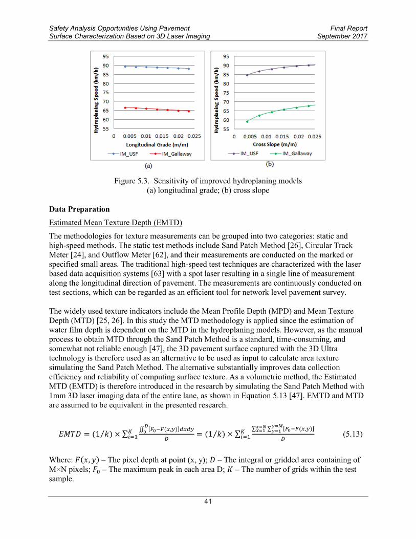
Safety Analysis Opportunities Using Pavement Final ReportSurface Characterization Based on 3D Laser Imaging September 2017
Hydroplaning Speed Estimation
15 samples of the calculated WFD EMTD and IMU data for hydroplaning speed prediction are given in Table 52 Gallaway model USF model the improved Gallaway model and the improved USF model are utilized to predict hydroplaning speed respectively as shown in Figure 10(a) Results indicate the predicted hydroplaning speeds from original Gallaway and USF model are approximately 140kmh and 165kmh respectively which are around 50kmh higher than those predicted from the improved Gallaway model (96kmh) and improved USF model (91kmh) The results also show as expected that the hydroplaning speeds at curves of the five horizontal curves in Figure 58(a) are lower than that on the straight road sections
Table 52 Sample 3D and IMU data for hydroplaning speed calculation Sample ID WFD (mm) EMTD (mm) Cross Slope () Longitudinal Grade ()
1 164 112 207 327 2 151 111 226 318 3 135 111 254 310 4 130 110 268 312 5 123 111 282 307 6 121 109 287 289 7 113 112 295 278 8 105 117 305 277 9 103 114 323 272 10 100 110 344 267 11 093 112 364 271 12 094 111 374 281 13 094 110 376 285 14 086 117 379 279 15 092 110 383 276
Potential Hydroplaning Segment Detection
Identification of locations with hydroplaning potential is based on the comparison of estimated hydroplaning speed with posted speed of the road section [47] At the test site speed limits are 80kmh on straight sections and 56kmh on road curves The average hydroplaning speeds calculated with the four models are used to detect potential hydroplaning segments shown in Figure 58(a) Since the predicted hydroplaning speeds at the five curves are higher than posted speed limit there is a low hydroplaning risk at the five curves for vehicles operating at speed limit However for several segments of the test site the predicted hydroplaning speeds are lower than the posted speed limit Therefore these segments can be identified as potential segments for increased hydroplaning risk as marked with red line in Figure 58(b) To minimize traffic crashes caused by hydroplaning highway agencies can post a reduced speed sign at these locations or take other remedial actions such as installing High-Friction Surface Treatment (HFST) [66]
46
Safety Analysis Opportunities Using Pavement Final ReportSurface Characterization Based on 3D Laser Imaging September 2017
Figure 58 Detection of potential hydroplaning risk (a) hydroplaning speed (b) increased hydroplaning potential segments
47
Safety Analysis Opportunities Using Pavement Final ReportSurface Characterization Based on 3D Laser Imaging September 2017
6 SUMMARY
The 3D Ultra laser imaging technology has the capability to collect pavement surface texture data at full-lane coverage at 1 mm resolution in all three dimensions at speed up to 60MPH This single-pass and complete lane coverage platform provides an ideal solution to evaluate pavement surface characteristics for safety analysis and many different data collection needs without interrupting traffic Furthermore it will saved cost by eliminating the need for maintenance of traffic
In this study the 3D Ultra laser imaging technology with necessary software tools are utilized for data collection and subsequent surface characterization and safety evaluation and analysis First the 1mm 3D data for 21 HFST sites in 11 states with a total of 41 sections are collected for each traffic lane at the posted highway speeds Pavement rutting and macro-texture data are calculated from collected 1mm 3D data sets while pavement friction data are collected using FHWAs fixed-slip continuous friction tester The measured surface characteristics on the HFST sites and untreated existing pavements are compared and paired t-tests are performed to determine the effectiveness of the HFST sites in improving surface characteristics It is evident that the HFST surfaces have statistically significant higher friction numbers and surface macro-texture MPD values than those on the adjacent pavements without HFST There exist several exceptions to such trend 2 sections for friction data and 5 sections for MPD data Multivariate analyses are conducted to investigate the impacts of five independent variables precipitation average temperature HFST installation age aggregate type and AADT on HFST friction performance Average temperature and HFST installation age are identified to have significantly impact on friction performance of HFST (FNHFST) and the ratio of friction on HFST to that on non-HFST (FN Ratio) Based on the trend between FN Ratio and installation age in general the benefit of HFST in friction effectiveness is lost after approximate 60 months (5 years) of service HFST sites using calcined bauxite aggregates exhibit higher friction performance than those using flints The regressional friction prediction models are therefore developed for HFST which can be used to predict the service life of HFST installation and aid decision making within a highway agency However it should be noted that the models donrsquot consider the pavement conditions before HFST application and HFST construction quality variations as the dependent variables due to the unavailability of data In addition detailed traffic data for ramps and each lane of sites with multiple lanes are not available and have to be estimated during the model development
Surface texture and friction are two primary characteristics for pavement safety evaluation Understanding their relationship is critical to reduce potential traffic crashes especially at wet conditions However the currently used texture indicators such as Mean Profile Depth (MPD) and Mean Texture Depth (MTD) are calculated restricted on either a small portion on pavement surface or single line of profile measurement and thus only reveal partial aspects of texture property With 1mm 3D laser texture data eight surface texture indicators are examined for their applications on pavement friction prediction The eight surface texture indicators are grouped into four categories amplitude parameters (including MPD SMTD RMS Skewness and Kurtosis) spacing parameters (TAR) hybrid parameters (SAR) and functional parameters (SBI) To avoid using two highly correlated texture indicators in the friction prediction model correlation analyses are conducted and found that 1) SMTD are highly correlated with MPD 2)
48
Safety Analysis Opportunities Using Pavement Final ReportSurface Characterization Based on 3D Laser Imaging September 2017
RMS is highly correlated with SAR As a result six texture indicators including MPD Skewness Kurtosis TAR SAR and SBI are adopted for the development of pavement friction prediction model using multivariate regression analysis The developed model can be used to predict pavement friction based on various texture indicators and may be beneficial in the continuous measurement and evaluation of pavement safety for the project- and network- level pavement surveys
The third application of using 1mm 3D Ultra data sets is to predict and evaluate pavement surface hydroplaning risk Considering the effects of flow path slope on vertical wheel load perpendicular to pavement surface and the resulting hydroplaning speed the Gallaway and USF models are modified for improvements in this study The sensitivity analysis shows that the hydroplaning speed is more sensitive to cross slope than longitudinal grade in the improved models A 3D based volumetric measuring method is used to calculate the estimated MTD based on the full-lane 1mm 3D data Subsequently IMU data and 3D data are combined to model vehicle movements on cross slopes Local rainfall intensity is obtained from NOAA precipitation database By considering effects of cross slope and longitudinal grade on wheel load and flow path length it is found that hydroplaning speed decreases with the increase of the longitudinal grade but increases with the increase of the cross slope The improved models predict lower hydroplaning speed than that from the original Gallaway and USF models An important future work is to use a combined slope based on longitudinal grade and cross slope to demonstrate the validity and effectiveness of the improved models
This study with field pavement applications has shown that the 1mm 3D Ultra which represent a form of 3D Laser imaging technology is promising in real-time pavement surface characterization and evaluation for both pavement and safety management at network and project level surveys It is anticipated that more data collection with more testing sites are to be performed to validate the new emerging 3D laser imaging technology as a single-pass and complete lane-coverage platform for multiple safety and pavement evaluation purposes In addition the long-term monitoring of the HFTS sites in multiple states is highly recommended due to the need to determine multi-year performance of the HFTS applications in terms of region pavement condition materials used geometric properties and other factors The recommended long-term study would provide much needed data for both design and construction of HFTS for its widespread adoption
49
Safety Analysis Opportunities Using Pavement Final ReportSurface Characterization Based on 3D Laser Imaging September 2017
REFERENCES
[1] Brimley B and Carlson P Using High Friction Surface Treatments to Improve Safety at Horizontal Curves Texas Transportation Institute httpd2dtl5nnlpfr0rcloudfrontnetttitamuedudocumentsTTI-2012-8pdf 2012 (accessed 150625)
[2] The Trans Tec Group INC Welcome to High Friction Roads httpwwwhighfrictionroadscom 2015 (accessed 150725)
[3] Bledsoe J Missouri Demonstration Project The Use of High-Friction Surface Treatments on Missouri Highways FHWA US Department of Transportation httpplan4operationsdotgovhflsummarypdf_2Missouri20High20Friction20Report 20draft20Finalpdf 2015 (accessed 150630)
[4] Moravec M High Friction Surface Treatments at High-Crash Horizontal Curves Arizona PavementsMaterials Conference Phoenix AZ httpwwwintransiastateedueventsmidcon2013documentspresentation-submissions3-C_61_08142013pdf 2013 (accessed 150630)
[5] South Dakota Department of Transportation (SDDOT) Accelerated Innovation Deployment (AID) Demonstration Project High Friction Surface Treatment httpwwwfhwadotgovacceleratinggrantspdfsSD_2014_AID_Grantpdf 2015 (accessed 150611)
[6] Bischoff D Investigative Study of the Italgrip TM System WI-04-08 Wisconsin Department of Transportation Madison WI httpwisdotresearchwigovwp-contentuploadswi-04-08italgrippdf 2008 (accessed 150620)
[7] Izeppi E Flintsch G and McGhee K Field Performance of High Friction Surfaces Publication FHWAVTRC 10-CR6 FHWA US Department of Transportation httpwwwvirginiadotorgvtrcmainonline_reportspdf10-cr6pdf 2010 (accessed 150615)
[8] Waters J High Friction Surfacing Failure Mechanisms 3rd International Surface Friction Conference Safer Road Surfaces ndash Saving Lives Gold Coast Australia 2011
[9] Wang Kelvin C P Elements of Automated Survey of Pavements and a 3D Methodology J mod transp Vol 19 pp 51-57 2011
[10] AASTHO Quantifying cracks in asphalt pavement surfaces from collected images utilizing automated methods AASHTO Designation PP67-10 American Association of State Highway and Transportation Officials Washington DC 2013
[11] AASTHO 2013 Standard Practice for Determining Pavement Deformation Parameters and Cross Slope from Collected Transverse Profiles AASHTO Designation PP69-10 American Association of State Highway and Transportation Officials Washington DC 2013
[12] Hall J W Smith K L Titus-Glover L Wambold J C Yager T J and Rado Z Guide for Pavement Friction Final Report for NCHRP Project 01-43 National Cooperative
50
Safety Analysis Opportunities Using Pavement Final ReportSurface Characterization Based on 3D Laser Imaging September 2017
Highway Research Program (NCHRP) Transportation Research Board (TRB) Washington DC 2009
[13] Ahammed MA and Tighe SL Concrete Pavement Surface Textures and Multivariables Frictional Performance Analysis a North American Case Study Can J Civil Eng Vol 35 727-738 2008
[14] Ergun M Iyinam S and Iyinam AF Prediction of Road Surface Friction Coefficient Using Only Macro- and Microtexture Measurements J Transp Eng Vol 131 pp 311-319 2005
[15] Flintsch GW et al The Little Book of Tire Pavement Friction Pavement Surface Properties Consortium httpssecurehostingvteduwwwappsvttivtedu1-pagersCSTI_FlintschThe20Little20Book20of20Tire20Pavement20Frictionpdf 2012 (accessed 150501)
[16] Henry J J NCHRP Synthesis 291 Evaluation of Pavement Friction Characteristics TRB National Research Council Washington DC 2000
[17] Ahammed MA and Tighe SL Effect of Short-term and Long-term Weather on Pavement Surface Friction Int J Na Res Tech Vol 3 pp 295-302 2010
[18] Luo Y Effect of Pavement Temperature on Frictional Properties of Hot-Mix-Asphalt Pavement Surfaces at the Virginia Smart Road MS Thesis Virginia Polytechnic Institute and State University Blacksburg Va 2003
[19] Fuents L G Investigation of the Factors Influencing Skid Resistance and the International Friction Index PhD Thesis University of South Florida Tampa FL 2009
[20] American Society for Testing and Materials (ASTM) ASTM E 867 Standard Terminology Relating to Vehicle-Pavement Systems ASTM Standard Practice E 867 Book of ASTM Standards Volume 0403 Philadelphia P A 2011
[21] International Standards Organization (ISO) Characterization of Pavement Texture using Surface Profiles ndash Part 1 Determination of Mean Profile Depth Acoustics ISO Standard 13473 International Standards Organization Geneva Switzerland 1998
[22] PIARC World Road Association Report of the Committee on Surface Characteristics In Proceeding of XVIII World Road Congress Brussels Belgium pp 13ndash19 1987
[23] Sandburg U Influence of Road Surface Texture on Traffic Characteristics Related to Environment Economy and Safety A State-of-the-Art Study Regarding Measures and Measuring Methods VTI Report 53A-1997 Swedish National Road Administration Borlange Sweden 1998
[24] American Society for Testing and Materials (ASTM) ASTM E 2157 Standard Test Method for Measuring Pavement Macro texture Properties Using the Circular Track Meter ASTM Standard Practice E 2157 Book of ASTM Standards Volume 0403 Philadelphia P A 2011
51
Safety Analysis Opportunities Using Pavement Final ReportSurface Characterization Based on 3D Laser Imaging September 2017
[25] American Society for Testing and Materials (ASTM) ASTM E 1845 Calculating Pavement Macro texture Profile Depth ASTM Standard Practice E 1845 Book of ASTM Standards Volume 0403 Philadelphia P A 2011
[26] American Society for Testing and Materials (ASTM) ASTM E 965 Standard Test Method for Measuring Pavement Macro texture Depth Using a Volumetric Technique ASTM Standard Practice E 965 Book of ASTM Standards Volume 0403 Philadelphia P A 2011
[27] McGhee K K amp Flintsch G W High-speed Texture Measurement of Pavements Virginia Transportation Research Council Charlottesville VA 2003
[28] Prowell B amp Hanson D Evaluation of Circular Texture Meter for Measuring Surface Texture of Pavements Transportation Research Record Journal of the Transportation Research Board No 1929 pp 88-96 2005
[29] Alvarez L amp Morel J M Formalization and Computational Aspects of Image Analysis Acta numerica Vol 3 pp 1-59 1994
[30] Gendy A E amp Shalaby A Mean Profile Depth of Pavement Surface Macrotexture Using Photometric Stereo Techniques Journal of Transportation Engineering Vol 133 No 7 pp 433-440 2007
[31] Kokkalis A and Panagouli O Fractal Evaluation of Pavement Skid Resistance Variations I Surface Wetting Chaos Solitons amp Fractals pp 1875-1890 1998
[32] American Society for Testing and Materials (ASTM) ASTM E 274 Standard Test Method for Skid Resistance of Paved Surfaces Using a Full-Scale Tire ASTM Standard Practice E 274 Book of ASTM Standards Volume 0403 Philadelphia P A 2011
[33] American Society for Testing and Materials (ASTM) ASTM E 303 Standard Test Method for Measuring Surface Frictional Properties Using a British Pendulum Tester ASTM Standard Practice E 303 Book of ASTM Standards Volume 0403 Philadelphia P A 2011
[34] Janoo VC and Horhonen C Performance Testing of Hot-Mix Asphalt Aggregates Special Report pp 99-20 1999
[35] Kuennen T Creating Friction Where Rubber Meets the Road Better Roads Vol 73 No 10 2003
[36] Leu MC Henry JJ Prediction of skid resistance as a function of speed from pavement texture measurements Transportation Research Record No 666 pp 7-13 1978
[37] Yager T J and Buhlmann F Macrotexture and Drainage Measurements on a Variety of Concrete and Asphalt Surfaces Pavement Surface Characteristics and Materials ASTM STP 763 pp 16-30 1982
[38] Rado Z Analysis of Texture Models PTI Report No 9510 Pennsylvania Transportation Institute (PTI) Penn State University State College Pennsylvania 1994
52
Safety Analysis Opportunities Using Pavement Final ReportSurface Characterization Based on 3D Laser Imaging September 2017
[39] Fwa T F Choo Y S and Liu Y (2003) Effect of Aggregate Spacing on Skid Resistance of Asphalt Pavement Journal of Transportation Engineering Vol 129 No 4 pp 420-426 2003
[40] Olek J Weiss W J and Garcia-Villarreal R Relating Surface Texture of Rigid Pavement with Noise and Skid Resistance Purdue University West Lafayette Indiana Report No SQDH-2004-1 (Final Report HL 2004-1) 2004
[41] Do MT Marsac P Delanne Y Prediction of Tirewet Road Friction from Road Surface Microtexture and Tire Rubber Properties In 5th International Symposium on Pavement Surface Characteristics Toronto 2004
[42] Ergun M Iyinam S amp Iyinam A F (2005) Prediction of Road Surface Friction Coefficient Using only Macro- and Micro texture Measurement Journal of transportation engineering Vol 131 No 4 pp 311-319 2005
[43] Kebrle J Walker R Texture measurement and friction estimation using laser data acquisition and neural networks In Proceedings of the 9th WSEAS International Conference on Mathematical and Computational Methods in Science and Engineering Trinidad and Tobago 2007
[44] Rezaei A Masad E Chowdhury A amp Harris P Predicting Asphalt Mixture Skid Resistance by Aggregate Characteristics and Gradation Transportation Research Record Journal of the Transportation Research Board No 2014 pp 24-33 2009
[45] American National Standards Institute Surface texture surface roughness waviness and lay American Society of Mechanical Engineers 1986
[46] Stout K J Sullivan PJ Dong WP Mainsah E Luo N Mathia T and Zahyouani H The development of methods for the characterization of roughness in three dimensions Commission of the European Communities 1993
[47] Luo Wenting Wang Kelvin C P Li Lin 2014 Surface Drainage Evaluation for Rigid Pavements Using IMU and 1 mm 3D Texture Data Transportation Research Record Journal of the Transportation Research Board Washington DC Pavement Management 2014 Volume 3 pp 121ndash128 2014
[48] Tsai C L Cai Z amp Wu X (1998) The examination of residual plots Statistica Sinica Vol 8 pp 445-465 1998
[49] Kumar SSantosh Anupam Kumar and FWA TF Analyzing effect of tire groove patterns on hydroplaning speed Journal of the Eastern Asia Society for Transportation Studies Vol 8 2009
[50] Khedr Safwan A and Breakah Tamer M Rutting parameters for asphalt concrete for different aggregate structures International Journal of Pavement Engineering Volume 12 Issue 1 pp 13-23 2011
53
Safety Analysis Opportunities Using Pavement Final ReportSurface Characterization Based on 3D Laser Imaging September 2017
[51] MISH Rohit Goyal Design and Analysis of Interceptor DrainsmdashEffect of Parameters ISH Journal of Hydraulic Engineering Volume 9 Issue 1 pp 61-71 2003
[52] Horne WB and RC Dreher Phenomena of Pneumatic Tire Hydroplaning NASA TN D-2-56 NASA Langley Research center NASA Hampton VA 1963
[53] Chesterton John Nancekivell Noel and Tunnicliffe Noel The use of the Gallaway Formula for Aquaplaning Evaluation in New Zealand Transit New Zealand and New Zealand Institute of Highway Technology (NZIHT) 8thAnnual Conference 2006
[54] Russam K and Ross NF The Depth of Rain Water on Road Surfaces Road Research Laboratory Ministry of Transport Report No LR 236 pp25 1968
[55] Gallaway B M et al Pavement and Geometric Design Criteria for Minimizing Hydroplaning Federal Highway Administration Report No FHWA-RD-79-31 1979
[56] Huebner RS et al PAVDRN Computer Model for Predicting Water Film Thickness and Potential or Hydroplaning on New and Reconditioned Pavements Transport Research Record 1599 pp 128-131 1996
[57] Gunaratne M Lu Q Yang J Hydroplaning on Multi Lane Facilities Report for Florida Department of Transportation Report No BDK84 977-14 2012
[58] Zhang Zhongjie Abu-Farsakh Murad Y and Tao Mingjiang Evaluation of trench backfills at highway cross-drains International Journal of Pavement Engineering Volume 6 Issue 2 pp77-87 2005
[59] Gallaway B M and Rose Gerry The Effects of Rainfall Intensity Pavement Cross Slope Surface Texture and Drainage Length on Pavement Water Depths Texas Transportation Institute Research Report No 138-5 1971
[60] Ong GP and Fwa TF Wet-pavement hydroplaning risk and skid-resistance Modeling ASCE Journal of Transportation Engineering Vol 133 No 10 2007
[61] Shafabakhsh GA Kashi E Effect of Aircraft Wheel Load and Configuration on Runway Damages Period Polytech Civil Eng Vol 59 No 1 pp 85-94 2015
[62] ASTM Measuring Pavement Texture Drainage Using an Outflow ASTM Standard Practice E 2380 Book of ASTM Standards Volume 0403 Philadelphia P A 2006
[63] ASTM Measuring Surface Frictional Properties Using the British Pendulum Tester ASTM Standard Practice E 303 Book of ASTM Standards Volume 0403 Philadelphia P A 2006
[64] Mekemson et al Method and Apparatus for Pavement Cross-slope Measurement Patent Application Publication Pub No US 20020013644 A1 2002
54
Safety Analysis Opportunities Using Pavement Final ReportSurface Characterization Based on 3D Laser Imaging September 2017
[65] NOAAs National Water Service Hydrometeorological Design Studies Center Precipitation Frequency Data Server (PFDS) httpdippernwsnoaagovhdscpfds Accessed on July 2014
[66] Shah Yogesh U Jain SS and Parida Manoranjan Evaluation of prioritization methods for effective pavement maintenance of urban roads International Journal of Pavement Engineering Volume 15 Issue 3 pp 238-250 2014
55
For More Information
Safety Analysis Opportunities Using Pavement Surface Characterization
Based on 3D Laser Imaging visit httpsafetyfhwadotgov
July 2017 FHWA-SA-17-046
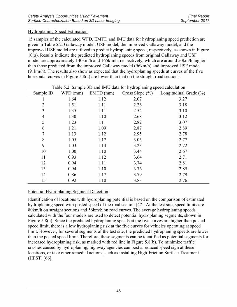
Safety Analysis Opportunities Using Pavement Final ReportSurface Characterization Based on 3D Laser Imaging September 2017
6 SUMMARY
The 3D Ultra laser imaging technology has the capability to collect pavement surface texture data at full-lane coverage at 1 mm resolution in all three dimensions at speed up to 60MPH This single-pass and complete lane coverage platform provides an ideal solution to evaluate pavement surface characteristics for safety analysis and many different data collection needs without interrupting traffic Furthermore it will saved cost by eliminating the need for maintenance of traffic
In this study the 3D Ultra laser imaging technology with necessary software tools are utilized for data collection and subsequent surface characterization and safety evaluation and analysis First the 1mm 3D data for 21 HFST sites in 11 states with a total of 41 sections are collected for each traffic lane at the posted highway speeds Pavement rutting and macro-texture data are calculated from collected 1mm 3D data sets while pavement friction data are collected using FHWAs fixed-slip continuous friction tester The measured surface characteristics on the HFST sites and untreated existing pavements are compared and paired t-tests are performed to determine the effectiveness of the HFST sites in improving surface characteristics It is evident that the HFST surfaces have statistically significant higher friction numbers and surface macro-texture MPD values than those on the adjacent pavements without HFST There exist several exceptions to such trend 2 sections for friction data and 5 sections for MPD data Multivariate analyses are conducted to investigate the impacts of five independent variables precipitation average temperature HFST installation age aggregate type and AADT on HFST friction performance Average temperature and HFST installation age are identified to have significantly impact on friction performance of HFST (FNHFST) and the ratio of friction on HFST to that on non-HFST (FN Ratio) Based on the trend between FN Ratio and installation age in general the benefit of HFST in friction effectiveness is lost after approximate 60 months (5 years) of service HFST sites using calcined bauxite aggregates exhibit higher friction performance than those using flints The regressional friction prediction models are therefore developed for HFST which can be used to predict the service life of HFST installation and aid decision making within a highway agency However it should be noted that the models donrsquot consider the pavement conditions before HFST application and HFST construction quality variations as the dependent variables due to the unavailability of data In addition detailed traffic data for ramps and each lane of sites with multiple lanes are not available and have to be estimated during the model development
Surface texture and friction are two primary characteristics for pavement safety evaluation Understanding their relationship is critical to reduce potential traffic crashes especially at wet conditions However the currently used texture indicators such as Mean Profile Depth (MPD) and Mean Texture Depth (MTD) are calculated restricted on either a small portion on pavement surface or single line of profile measurement and thus only reveal partial aspects of texture property With 1mm 3D laser texture data eight surface texture indicators are examined for their applications on pavement friction prediction The eight surface texture indicators are grouped into four categories amplitude parameters (including MPD SMTD RMS Skewness and Kurtosis) spacing parameters (TAR) hybrid parameters (SAR) and functional parameters (SBI) To avoid using two highly correlated texture indicators in the friction prediction model correlation analyses are conducted and found that 1) SMTD are highly correlated with MPD 2)
48
Safety Analysis Opportunities Using Pavement Final ReportSurface Characterization Based on 3D Laser Imaging September 2017
RMS is highly correlated with SAR As a result six texture indicators including MPD Skewness Kurtosis TAR SAR and SBI are adopted for the development of pavement friction prediction model using multivariate regression analysis The developed model can be used to predict pavement friction based on various texture indicators and may be beneficial in the continuous measurement and evaluation of pavement safety for the project- and network- level pavement surveys
The third application of using 1mm 3D Ultra data sets is to predict and evaluate pavement surface hydroplaning risk Considering the effects of flow path slope on vertical wheel load perpendicular to pavement surface and the resulting hydroplaning speed the Gallaway and USF models are modified for improvements in this study The sensitivity analysis shows that the hydroplaning speed is more sensitive to cross slope than longitudinal grade in the improved models A 3D based volumetric measuring method is used to calculate the estimated MTD based on the full-lane 1mm 3D data Subsequently IMU data and 3D data are combined to model vehicle movements on cross slopes Local rainfall intensity is obtained from NOAA precipitation database By considering effects of cross slope and longitudinal grade on wheel load and flow path length it is found that hydroplaning speed decreases with the increase of the longitudinal grade but increases with the increase of the cross slope The improved models predict lower hydroplaning speed than that from the original Gallaway and USF models An important future work is to use a combined slope based on longitudinal grade and cross slope to demonstrate the validity and effectiveness of the improved models
This study with field pavement applications has shown that the 1mm 3D Ultra which represent a form of 3D Laser imaging technology is promising in real-time pavement surface characterization and evaluation for both pavement and safety management at network and project level surveys It is anticipated that more data collection with more testing sites are to be performed to validate the new emerging 3D laser imaging technology as a single-pass and complete lane-coverage platform for multiple safety and pavement evaluation purposes In addition the long-term monitoring of the HFTS sites in multiple states is highly recommended due to the need to determine multi-year performance of the HFTS applications in terms of region pavement condition materials used geometric properties and other factors The recommended long-term study would provide much needed data for both design and construction of HFTS for its widespread adoption
49
Safety Analysis Opportunities Using Pavement Final ReportSurface Characterization Based on 3D Laser Imaging September 2017
REFERENCES
[1] Brimley B and Carlson P Using High Friction Surface Treatments to Improve Safety at Horizontal Curves Texas Transportation Institute httpd2dtl5nnlpfr0rcloudfrontnetttitamuedudocumentsTTI-2012-8pdf 2012 (accessed 150625)
[2] The Trans Tec Group INC Welcome to High Friction Roads httpwwwhighfrictionroadscom 2015 (accessed 150725)
[3] Bledsoe J Missouri Demonstration Project The Use of High-Friction Surface Treatments on Missouri Highways FHWA US Department of Transportation httpplan4operationsdotgovhflsummarypdf_2Missouri20High20Friction20Report 20draft20Finalpdf 2015 (accessed 150630)
[4] Moravec M High Friction Surface Treatments at High-Crash Horizontal Curves Arizona PavementsMaterials Conference Phoenix AZ httpwwwintransiastateedueventsmidcon2013documentspresentation-submissions3-C_61_08142013pdf 2013 (accessed 150630)
[5] South Dakota Department of Transportation (SDDOT) Accelerated Innovation Deployment (AID) Demonstration Project High Friction Surface Treatment httpwwwfhwadotgovacceleratinggrantspdfsSD_2014_AID_Grantpdf 2015 (accessed 150611)
[6] Bischoff D Investigative Study of the Italgrip TM System WI-04-08 Wisconsin Department of Transportation Madison WI httpwisdotresearchwigovwp-contentuploadswi-04-08italgrippdf 2008 (accessed 150620)
[7] Izeppi E Flintsch G and McGhee K Field Performance of High Friction Surfaces Publication FHWAVTRC 10-CR6 FHWA US Department of Transportation httpwwwvirginiadotorgvtrcmainonline_reportspdf10-cr6pdf 2010 (accessed 150615)
[8] Waters J High Friction Surfacing Failure Mechanisms 3rd International Surface Friction Conference Safer Road Surfaces ndash Saving Lives Gold Coast Australia 2011
[9] Wang Kelvin C P Elements of Automated Survey of Pavements and a 3D Methodology J mod transp Vol 19 pp 51-57 2011
[10] AASTHO Quantifying cracks in asphalt pavement surfaces from collected images utilizing automated methods AASHTO Designation PP67-10 American Association of State Highway and Transportation Officials Washington DC 2013
[11] AASTHO 2013 Standard Practice for Determining Pavement Deformation Parameters and Cross Slope from Collected Transverse Profiles AASHTO Designation PP69-10 American Association of State Highway and Transportation Officials Washington DC 2013
[12] Hall J W Smith K L Titus-Glover L Wambold J C Yager T J and Rado Z Guide for Pavement Friction Final Report for NCHRP Project 01-43 National Cooperative
50
Safety Analysis Opportunities Using Pavement Final ReportSurface Characterization Based on 3D Laser Imaging September 2017
Highway Research Program (NCHRP) Transportation Research Board (TRB) Washington DC 2009
[13] Ahammed MA and Tighe SL Concrete Pavement Surface Textures and Multivariables Frictional Performance Analysis a North American Case Study Can J Civil Eng Vol 35 727-738 2008
[14] Ergun M Iyinam S and Iyinam AF Prediction of Road Surface Friction Coefficient Using Only Macro- and Microtexture Measurements J Transp Eng Vol 131 pp 311-319 2005
[15] Flintsch GW et al The Little Book of Tire Pavement Friction Pavement Surface Properties Consortium httpssecurehostingvteduwwwappsvttivtedu1-pagersCSTI_FlintschThe20Little20Book20of20Tire20Pavement20Frictionpdf 2012 (accessed 150501)
[16] Henry J J NCHRP Synthesis 291 Evaluation of Pavement Friction Characteristics TRB National Research Council Washington DC 2000
[17] Ahammed MA and Tighe SL Effect of Short-term and Long-term Weather on Pavement Surface Friction Int J Na Res Tech Vol 3 pp 295-302 2010
[18] Luo Y Effect of Pavement Temperature on Frictional Properties of Hot-Mix-Asphalt Pavement Surfaces at the Virginia Smart Road MS Thesis Virginia Polytechnic Institute and State University Blacksburg Va 2003
[19] Fuents L G Investigation of the Factors Influencing Skid Resistance and the International Friction Index PhD Thesis University of South Florida Tampa FL 2009
[20] American Society for Testing and Materials (ASTM) ASTM E 867 Standard Terminology Relating to Vehicle-Pavement Systems ASTM Standard Practice E 867 Book of ASTM Standards Volume 0403 Philadelphia P A 2011
[21] International Standards Organization (ISO) Characterization of Pavement Texture using Surface Profiles ndash Part 1 Determination of Mean Profile Depth Acoustics ISO Standard 13473 International Standards Organization Geneva Switzerland 1998
[22] PIARC World Road Association Report of the Committee on Surface Characteristics In Proceeding of XVIII World Road Congress Brussels Belgium pp 13ndash19 1987
[23] Sandburg U Influence of Road Surface Texture on Traffic Characteristics Related to Environment Economy and Safety A State-of-the-Art Study Regarding Measures and Measuring Methods VTI Report 53A-1997 Swedish National Road Administration Borlange Sweden 1998
[24] American Society for Testing and Materials (ASTM) ASTM E 2157 Standard Test Method for Measuring Pavement Macro texture Properties Using the Circular Track Meter ASTM Standard Practice E 2157 Book of ASTM Standards Volume 0403 Philadelphia P A 2011
51
Safety Analysis Opportunities Using Pavement Final ReportSurface Characterization Based on 3D Laser Imaging September 2017
[25] American Society for Testing and Materials (ASTM) ASTM E 1845 Calculating Pavement Macro texture Profile Depth ASTM Standard Practice E 1845 Book of ASTM Standards Volume 0403 Philadelphia P A 2011
[26] American Society for Testing and Materials (ASTM) ASTM E 965 Standard Test Method for Measuring Pavement Macro texture Depth Using a Volumetric Technique ASTM Standard Practice E 965 Book of ASTM Standards Volume 0403 Philadelphia P A 2011
[27] McGhee K K amp Flintsch G W High-speed Texture Measurement of Pavements Virginia Transportation Research Council Charlottesville VA 2003
[28] Prowell B amp Hanson D Evaluation of Circular Texture Meter for Measuring Surface Texture of Pavements Transportation Research Record Journal of the Transportation Research Board No 1929 pp 88-96 2005
[29] Alvarez L amp Morel J M Formalization and Computational Aspects of Image Analysis Acta numerica Vol 3 pp 1-59 1994
[30] Gendy A E amp Shalaby A Mean Profile Depth of Pavement Surface Macrotexture Using Photometric Stereo Techniques Journal of Transportation Engineering Vol 133 No 7 pp 433-440 2007
[31] Kokkalis A and Panagouli O Fractal Evaluation of Pavement Skid Resistance Variations I Surface Wetting Chaos Solitons amp Fractals pp 1875-1890 1998
[32] American Society for Testing and Materials (ASTM) ASTM E 274 Standard Test Method for Skid Resistance of Paved Surfaces Using a Full-Scale Tire ASTM Standard Practice E 274 Book of ASTM Standards Volume 0403 Philadelphia P A 2011
[33] American Society for Testing and Materials (ASTM) ASTM E 303 Standard Test Method for Measuring Surface Frictional Properties Using a British Pendulum Tester ASTM Standard Practice E 303 Book of ASTM Standards Volume 0403 Philadelphia P A 2011
[34] Janoo VC and Horhonen C Performance Testing of Hot-Mix Asphalt Aggregates Special Report pp 99-20 1999
[35] Kuennen T Creating Friction Where Rubber Meets the Road Better Roads Vol 73 No 10 2003
[36] Leu MC Henry JJ Prediction of skid resistance as a function of speed from pavement texture measurements Transportation Research Record No 666 pp 7-13 1978
[37] Yager T J and Buhlmann F Macrotexture and Drainage Measurements on a Variety of Concrete and Asphalt Surfaces Pavement Surface Characteristics and Materials ASTM STP 763 pp 16-30 1982
[38] Rado Z Analysis of Texture Models PTI Report No 9510 Pennsylvania Transportation Institute (PTI) Penn State University State College Pennsylvania 1994
52
Safety Analysis Opportunities Using Pavement Final ReportSurface Characterization Based on 3D Laser Imaging September 2017
[39] Fwa T F Choo Y S and Liu Y (2003) Effect of Aggregate Spacing on Skid Resistance of Asphalt Pavement Journal of Transportation Engineering Vol 129 No 4 pp 420-426 2003
[40] Olek J Weiss W J and Garcia-Villarreal R Relating Surface Texture of Rigid Pavement with Noise and Skid Resistance Purdue University West Lafayette Indiana Report No SQDH-2004-1 (Final Report HL 2004-1) 2004
[41] Do MT Marsac P Delanne Y Prediction of Tirewet Road Friction from Road Surface Microtexture and Tire Rubber Properties In 5th International Symposium on Pavement Surface Characteristics Toronto 2004
[42] Ergun M Iyinam S amp Iyinam A F (2005) Prediction of Road Surface Friction Coefficient Using only Macro- and Micro texture Measurement Journal of transportation engineering Vol 131 No 4 pp 311-319 2005
[43] Kebrle J Walker R Texture measurement and friction estimation using laser data acquisition and neural networks In Proceedings of the 9th WSEAS International Conference on Mathematical and Computational Methods in Science and Engineering Trinidad and Tobago 2007
[44] Rezaei A Masad E Chowdhury A amp Harris P Predicting Asphalt Mixture Skid Resistance by Aggregate Characteristics and Gradation Transportation Research Record Journal of the Transportation Research Board No 2014 pp 24-33 2009
[45] American National Standards Institute Surface texture surface roughness waviness and lay American Society of Mechanical Engineers 1986
[46] Stout K J Sullivan PJ Dong WP Mainsah E Luo N Mathia T and Zahyouani H The development of methods for the characterization of roughness in three dimensions Commission of the European Communities 1993
[47] Luo Wenting Wang Kelvin C P Li Lin 2014 Surface Drainage Evaluation for Rigid Pavements Using IMU and 1 mm 3D Texture Data Transportation Research Record Journal of the Transportation Research Board Washington DC Pavement Management 2014 Volume 3 pp 121ndash128 2014
[48] Tsai C L Cai Z amp Wu X (1998) The examination of residual plots Statistica Sinica Vol 8 pp 445-465 1998
[49] Kumar SSantosh Anupam Kumar and FWA TF Analyzing effect of tire groove patterns on hydroplaning speed Journal of the Eastern Asia Society for Transportation Studies Vol 8 2009
[50] Khedr Safwan A and Breakah Tamer M Rutting parameters for asphalt concrete for different aggregate structures International Journal of Pavement Engineering Volume 12 Issue 1 pp 13-23 2011
53
Safety Analysis Opportunities Using Pavement Final ReportSurface Characterization Based on 3D Laser Imaging September 2017
[51] MISH Rohit Goyal Design and Analysis of Interceptor DrainsmdashEffect of Parameters ISH Journal of Hydraulic Engineering Volume 9 Issue 1 pp 61-71 2003
[52] Horne WB and RC Dreher Phenomena of Pneumatic Tire Hydroplaning NASA TN D-2-56 NASA Langley Research center NASA Hampton VA 1963
[53] Chesterton John Nancekivell Noel and Tunnicliffe Noel The use of the Gallaway Formula for Aquaplaning Evaluation in New Zealand Transit New Zealand and New Zealand Institute of Highway Technology (NZIHT) 8thAnnual Conference 2006
[54] Russam K and Ross NF The Depth of Rain Water on Road Surfaces Road Research Laboratory Ministry of Transport Report No LR 236 pp25 1968
[55] Gallaway B M et al Pavement and Geometric Design Criteria for Minimizing Hydroplaning Federal Highway Administration Report No FHWA-RD-79-31 1979
[56] Huebner RS et al PAVDRN Computer Model for Predicting Water Film Thickness and Potential or Hydroplaning on New and Reconditioned Pavements Transport Research Record 1599 pp 128-131 1996
[57] Gunaratne M Lu Q Yang J Hydroplaning on Multi Lane Facilities Report for Florida Department of Transportation Report No BDK84 977-14 2012
[58] Zhang Zhongjie Abu-Farsakh Murad Y and Tao Mingjiang Evaluation of trench backfills at highway cross-drains International Journal of Pavement Engineering Volume 6 Issue 2 pp77-87 2005
[59] Gallaway B M and Rose Gerry The Effects of Rainfall Intensity Pavement Cross Slope Surface Texture and Drainage Length on Pavement Water Depths Texas Transportation Institute Research Report No 138-5 1971
[60] Ong GP and Fwa TF Wet-pavement hydroplaning risk and skid-resistance Modeling ASCE Journal of Transportation Engineering Vol 133 No 10 2007
[61] Shafabakhsh GA Kashi E Effect of Aircraft Wheel Load and Configuration on Runway Damages Period Polytech Civil Eng Vol 59 No 1 pp 85-94 2015
[62] ASTM Measuring Pavement Texture Drainage Using an Outflow ASTM Standard Practice E 2380 Book of ASTM Standards Volume 0403 Philadelphia P A 2006
[63] ASTM Measuring Surface Frictional Properties Using the British Pendulum Tester ASTM Standard Practice E 303 Book of ASTM Standards Volume 0403 Philadelphia P A 2006
[64] Mekemson et al Method and Apparatus for Pavement Cross-slope Measurement Patent Application Publication Pub No US 20020013644 A1 2002
54
Safety Analysis Opportunities Using Pavement Final ReportSurface Characterization Based on 3D Laser Imaging September 2017
[65] NOAAs National Water Service Hydrometeorological Design Studies Center Precipitation Frequency Data Server (PFDS) httpdippernwsnoaagovhdscpfds Accessed on July 2014
[66] Shah Yogesh U Jain SS and Parida Manoranjan Evaluation of prioritization methods for effective pavement maintenance of urban roads International Journal of Pavement Engineering Volume 15 Issue 3 pp 238-250 2014
55
For More Information
Safety Analysis Opportunities Using Pavement Surface Characterization
Based on 3D Laser Imaging visit httpsafetyfhwadotgov
July 2017 FHWA-SA-17-046
Safety Analysis Opportunities Using Pavement Final ReportSurface Characterization Based on 3D Laser Imaging September 2017
RMS is highly correlated with SAR As a result six texture indicators including MPD Skewness Kurtosis TAR SAR and SBI are adopted for the development of pavement friction prediction model using multivariate regression analysis The developed model can be used to predict pavement friction based on various texture indicators and may be beneficial in the continuous measurement and evaluation of pavement safety for the project- and network- level pavement surveys
The third application of using 1mm 3D Ultra data sets is to predict and evaluate pavement surface hydroplaning risk Considering the effects of flow path slope on vertical wheel load perpendicular to pavement surface and the resulting hydroplaning speed the Gallaway and USF models are modified for improvements in this study The sensitivity analysis shows that the hydroplaning speed is more sensitive to cross slope than longitudinal grade in the improved models A 3D based volumetric measuring method is used to calculate the estimated MTD based on the full-lane 1mm 3D data Subsequently IMU data and 3D data are combined to model vehicle movements on cross slopes Local rainfall intensity is obtained from NOAA precipitation database By considering effects of cross slope and longitudinal grade on wheel load and flow path length it is found that hydroplaning speed decreases with the increase of the longitudinal grade but increases with the increase of the cross slope The improved models predict lower hydroplaning speed than that from the original Gallaway and USF models An important future work is to use a combined slope based on longitudinal grade and cross slope to demonstrate the validity and effectiveness of the improved models
This study with field pavement applications has shown that the 1mm 3D Ultra which represent a form of 3D Laser imaging technology is promising in real-time pavement surface characterization and evaluation for both pavement and safety management at network and project level surveys It is anticipated that more data collection with more testing sites are to be performed to validate the new emerging 3D laser imaging technology as a single-pass and complete lane-coverage platform for multiple safety and pavement evaluation purposes In addition the long-term monitoring of the HFTS sites in multiple states is highly recommended due to the need to determine multi-year performance of the HFTS applications in terms of region pavement condition materials used geometric properties and other factors The recommended long-term study would provide much needed data for both design and construction of HFTS for its widespread adoption
49
Safety Analysis Opportunities Using Pavement Final ReportSurface Characterization Based on 3D Laser Imaging September 2017
REFERENCES
[1] Brimley B and Carlson P Using High Friction Surface Treatments to Improve Safety at Horizontal Curves Texas Transportation Institute httpd2dtl5nnlpfr0rcloudfrontnetttitamuedudocumentsTTI-2012-8pdf 2012 (accessed 150625)
[2] The Trans Tec Group INC Welcome to High Friction Roads httpwwwhighfrictionroadscom 2015 (accessed 150725)
[3] Bledsoe J Missouri Demonstration Project The Use of High-Friction Surface Treatments on Missouri Highways FHWA US Department of Transportation httpplan4operationsdotgovhflsummarypdf_2Missouri20High20Friction20Report 20draft20Finalpdf 2015 (accessed 150630)
[4] Moravec M High Friction Surface Treatments at High-Crash Horizontal Curves Arizona PavementsMaterials Conference Phoenix AZ httpwwwintransiastateedueventsmidcon2013documentspresentation-submissions3-C_61_08142013pdf 2013 (accessed 150630)
[5] South Dakota Department of Transportation (SDDOT) Accelerated Innovation Deployment (AID) Demonstration Project High Friction Surface Treatment httpwwwfhwadotgovacceleratinggrantspdfsSD_2014_AID_Grantpdf 2015 (accessed 150611)
[6] Bischoff D Investigative Study of the Italgrip TM System WI-04-08 Wisconsin Department of Transportation Madison WI httpwisdotresearchwigovwp-contentuploadswi-04-08italgrippdf 2008 (accessed 150620)
[7] Izeppi E Flintsch G and McGhee K Field Performance of High Friction Surfaces Publication FHWAVTRC 10-CR6 FHWA US Department of Transportation httpwwwvirginiadotorgvtrcmainonline_reportspdf10-cr6pdf 2010 (accessed 150615)
[8] Waters J High Friction Surfacing Failure Mechanisms 3rd International Surface Friction Conference Safer Road Surfaces ndash Saving Lives Gold Coast Australia 2011
[9] Wang Kelvin C P Elements of Automated Survey of Pavements and a 3D Methodology J mod transp Vol 19 pp 51-57 2011
[10] AASTHO Quantifying cracks in asphalt pavement surfaces from collected images utilizing automated methods AASHTO Designation PP67-10 American Association of State Highway and Transportation Officials Washington DC 2013
[11] AASTHO 2013 Standard Practice for Determining Pavement Deformation Parameters and Cross Slope from Collected Transverse Profiles AASHTO Designation PP69-10 American Association of State Highway and Transportation Officials Washington DC 2013
[12] Hall J W Smith K L Titus-Glover L Wambold J C Yager T J and Rado Z Guide for Pavement Friction Final Report for NCHRP Project 01-43 National Cooperative
50
Safety Analysis Opportunities Using Pavement Final ReportSurface Characterization Based on 3D Laser Imaging September 2017
Highway Research Program (NCHRP) Transportation Research Board (TRB) Washington DC 2009
[13] Ahammed MA and Tighe SL Concrete Pavement Surface Textures and Multivariables Frictional Performance Analysis a North American Case Study Can J Civil Eng Vol 35 727-738 2008
[14] Ergun M Iyinam S and Iyinam AF Prediction of Road Surface Friction Coefficient Using Only Macro- and Microtexture Measurements J Transp Eng Vol 131 pp 311-319 2005
[15] Flintsch GW et al The Little Book of Tire Pavement Friction Pavement Surface Properties Consortium httpssecurehostingvteduwwwappsvttivtedu1-pagersCSTI_FlintschThe20Little20Book20of20Tire20Pavement20Frictionpdf 2012 (accessed 150501)
[16] Henry J J NCHRP Synthesis 291 Evaluation of Pavement Friction Characteristics TRB National Research Council Washington DC 2000
[17] Ahammed MA and Tighe SL Effect of Short-term and Long-term Weather on Pavement Surface Friction Int J Na Res Tech Vol 3 pp 295-302 2010
[18] Luo Y Effect of Pavement Temperature on Frictional Properties of Hot-Mix-Asphalt Pavement Surfaces at the Virginia Smart Road MS Thesis Virginia Polytechnic Institute and State University Blacksburg Va 2003
[19] Fuents L G Investigation of the Factors Influencing Skid Resistance and the International Friction Index PhD Thesis University of South Florida Tampa FL 2009
[20] American Society for Testing and Materials (ASTM) ASTM E 867 Standard Terminology Relating to Vehicle-Pavement Systems ASTM Standard Practice E 867 Book of ASTM Standards Volume 0403 Philadelphia P A 2011
[21] International Standards Organization (ISO) Characterization of Pavement Texture using Surface Profiles ndash Part 1 Determination of Mean Profile Depth Acoustics ISO Standard 13473 International Standards Organization Geneva Switzerland 1998
[22] PIARC World Road Association Report of the Committee on Surface Characteristics In Proceeding of XVIII World Road Congress Brussels Belgium pp 13ndash19 1987
[23] Sandburg U Influence of Road Surface Texture on Traffic Characteristics Related to Environment Economy and Safety A State-of-the-Art Study Regarding Measures and Measuring Methods VTI Report 53A-1997 Swedish National Road Administration Borlange Sweden 1998
[24] American Society for Testing and Materials (ASTM) ASTM E 2157 Standard Test Method for Measuring Pavement Macro texture Properties Using the Circular Track Meter ASTM Standard Practice E 2157 Book of ASTM Standards Volume 0403 Philadelphia P A 2011
51
Safety Analysis Opportunities Using Pavement Final ReportSurface Characterization Based on 3D Laser Imaging September 2017
[25] American Society for Testing and Materials (ASTM) ASTM E 1845 Calculating Pavement Macro texture Profile Depth ASTM Standard Practice E 1845 Book of ASTM Standards Volume 0403 Philadelphia P A 2011
[26] American Society for Testing and Materials (ASTM) ASTM E 965 Standard Test Method for Measuring Pavement Macro texture Depth Using a Volumetric Technique ASTM Standard Practice E 965 Book of ASTM Standards Volume 0403 Philadelphia P A 2011
[27] McGhee K K amp Flintsch G W High-speed Texture Measurement of Pavements Virginia Transportation Research Council Charlottesville VA 2003
[28] Prowell B amp Hanson D Evaluation of Circular Texture Meter for Measuring Surface Texture of Pavements Transportation Research Record Journal of the Transportation Research Board No 1929 pp 88-96 2005
[29] Alvarez L amp Morel J M Formalization and Computational Aspects of Image Analysis Acta numerica Vol 3 pp 1-59 1994
[30] Gendy A E amp Shalaby A Mean Profile Depth of Pavement Surface Macrotexture Using Photometric Stereo Techniques Journal of Transportation Engineering Vol 133 No 7 pp 433-440 2007
[31] Kokkalis A and Panagouli O Fractal Evaluation of Pavement Skid Resistance Variations I Surface Wetting Chaos Solitons amp Fractals pp 1875-1890 1998
[32] American Society for Testing and Materials (ASTM) ASTM E 274 Standard Test Method for Skid Resistance of Paved Surfaces Using a Full-Scale Tire ASTM Standard Practice E 274 Book of ASTM Standards Volume 0403 Philadelphia P A 2011
[33] American Society for Testing and Materials (ASTM) ASTM E 303 Standard Test Method for Measuring Surface Frictional Properties Using a British Pendulum Tester ASTM Standard Practice E 303 Book of ASTM Standards Volume 0403 Philadelphia P A 2011
[34] Janoo VC and Horhonen C Performance Testing of Hot-Mix Asphalt Aggregates Special Report pp 99-20 1999
[35] Kuennen T Creating Friction Where Rubber Meets the Road Better Roads Vol 73 No 10 2003
[36] Leu MC Henry JJ Prediction of skid resistance as a function of speed from pavement texture measurements Transportation Research Record No 666 pp 7-13 1978
[37] Yager T J and Buhlmann F Macrotexture and Drainage Measurements on a Variety of Concrete and Asphalt Surfaces Pavement Surface Characteristics and Materials ASTM STP 763 pp 16-30 1982
[38] Rado Z Analysis of Texture Models PTI Report No 9510 Pennsylvania Transportation Institute (PTI) Penn State University State College Pennsylvania 1994
52
Safety Analysis Opportunities Using Pavement Final ReportSurface Characterization Based on 3D Laser Imaging September 2017
[39] Fwa T F Choo Y S and Liu Y (2003) Effect of Aggregate Spacing on Skid Resistance of Asphalt Pavement Journal of Transportation Engineering Vol 129 No 4 pp 420-426 2003
[40] Olek J Weiss W J and Garcia-Villarreal R Relating Surface Texture of Rigid Pavement with Noise and Skid Resistance Purdue University West Lafayette Indiana Report No SQDH-2004-1 (Final Report HL 2004-1) 2004
[41] Do MT Marsac P Delanne Y Prediction of Tirewet Road Friction from Road Surface Microtexture and Tire Rubber Properties In 5th International Symposium on Pavement Surface Characteristics Toronto 2004
[42] Ergun M Iyinam S amp Iyinam A F (2005) Prediction of Road Surface Friction Coefficient Using only Macro- and Micro texture Measurement Journal of transportation engineering Vol 131 No 4 pp 311-319 2005
[43] Kebrle J Walker R Texture measurement and friction estimation using laser data acquisition and neural networks In Proceedings of the 9th WSEAS International Conference on Mathematical and Computational Methods in Science and Engineering Trinidad and Tobago 2007
[44] Rezaei A Masad E Chowdhury A amp Harris P Predicting Asphalt Mixture Skid Resistance by Aggregate Characteristics and Gradation Transportation Research Record Journal of the Transportation Research Board No 2014 pp 24-33 2009
[45] American National Standards Institute Surface texture surface roughness waviness and lay American Society of Mechanical Engineers 1986
[46] Stout K J Sullivan PJ Dong WP Mainsah E Luo N Mathia T and Zahyouani H The development of methods for the characterization of roughness in three dimensions Commission of the European Communities 1993
[47] Luo Wenting Wang Kelvin C P Li Lin 2014 Surface Drainage Evaluation for Rigid Pavements Using IMU and 1 mm 3D Texture Data Transportation Research Record Journal of the Transportation Research Board Washington DC Pavement Management 2014 Volume 3 pp 121ndash128 2014
[48] Tsai C L Cai Z amp Wu X (1998) The examination of residual plots Statistica Sinica Vol 8 pp 445-465 1998
[49] Kumar SSantosh Anupam Kumar and FWA TF Analyzing effect of tire groove patterns on hydroplaning speed Journal of the Eastern Asia Society for Transportation Studies Vol 8 2009
[50] Khedr Safwan A and Breakah Tamer M Rutting parameters for asphalt concrete for different aggregate structures International Journal of Pavement Engineering Volume 12 Issue 1 pp 13-23 2011
53
Safety Analysis Opportunities Using Pavement Final ReportSurface Characterization Based on 3D Laser Imaging September 2017
[51] MISH Rohit Goyal Design and Analysis of Interceptor DrainsmdashEffect of Parameters ISH Journal of Hydraulic Engineering Volume 9 Issue 1 pp 61-71 2003
[52] Horne WB and RC Dreher Phenomena of Pneumatic Tire Hydroplaning NASA TN D-2-56 NASA Langley Research center NASA Hampton VA 1963
[53] Chesterton John Nancekivell Noel and Tunnicliffe Noel The use of the Gallaway Formula for Aquaplaning Evaluation in New Zealand Transit New Zealand and New Zealand Institute of Highway Technology (NZIHT) 8thAnnual Conference 2006
[54] Russam K and Ross NF The Depth of Rain Water on Road Surfaces Road Research Laboratory Ministry of Transport Report No LR 236 pp25 1968
[55] Gallaway B M et al Pavement and Geometric Design Criteria for Minimizing Hydroplaning Federal Highway Administration Report No FHWA-RD-79-31 1979
[56] Huebner RS et al PAVDRN Computer Model for Predicting Water Film Thickness and Potential or Hydroplaning on New and Reconditioned Pavements Transport Research Record 1599 pp 128-131 1996
[57] Gunaratne M Lu Q Yang J Hydroplaning on Multi Lane Facilities Report for Florida Department of Transportation Report No BDK84 977-14 2012
[58] Zhang Zhongjie Abu-Farsakh Murad Y and Tao Mingjiang Evaluation of trench backfills at highway cross-drains International Journal of Pavement Engineering Volume 6 Issue 2 pp77-87 2005
[59] Gallaway B M and Rose Gerry The Effects of Rainfall Intensity Pavement Cross Slope Surface Texture and Drainage Length on Pavement Water Depths Texas Transportation Institute Research Report No 138-5 1971
[60] Ong GP and Fwa TF Wet-pavement hydroplaning risk and skid-resistance Modeling ASCE Journal of Transportation Engineering Vol 133 No 10 2007
[61] Shafabakhsh GA Kashi E Effect of Aircraft Wheel Load and Configuration on Runway Damages Period Polytech Civil Eng Vol 59 No 1 pp 85-94 2015
[62] ASTM Measuring Pavement Texture Drainage Using an Outflow ASTM Standard Practice E 2380 Book of ASTM Standards Volume 0403 Philadelphia P A 2006
[63] ASTM Measuring Surface Frictional Properties Using the British Pendulum Tester ASTM Standard Practice E 303 Book of ASTM Standards Volume 0403 Philadelphia P A 2006
[64] Mekemson et al Method and Apparatus for Pavement Cross-slope Measurement Patent Application Publication Pub No US 20020013644 A1 2002
54
Safety Analysis Opportunities Using Pavement Final ReportSurface Characterization Based on 3D Laser Imaging September 2017
[65] NOAAs National Water Service Hydrometeorological Design Studies Center Precipitation Frequency Data Server (PFDS) httpdippernwsnoaagovhdscpfds Accessed on July 2014
[66] Shah Yogesh U Jain SS and Parida Manoranjan Evaluation of prioritization methods for effective pavement maintenance of urban roads International Journal of Pavement Engineering Volume 15 Issue 3 pp 238-250 2014
55
For More Information
Safety Analysis Opportunities Using Pavement Surface Characterization
Based on 3D Laser Imaging visit httpsafetyfhwadotgov
July 2017 FHWA-SA-17-046

Safety Analysis Opportunities Using Pavement Final ReportSurface Characterization Based on 3D Laser Imaging September 2017
[65] NOAAs National Water Service Hydrometeorological Design Studies Center Precipitation Frequency Data Server (PFDS) httpdippernwsnoaagovhdscpfds Accessed on July 2014
[66] Shah Yogesh U Jain SS and Parida Manoranjan Evaluation of prioritization methods for effective pavement maintenance of urban roads International Journal of Pavement Engineering Volume 15 Issue 3 pp 238-250 2014
55
For More Information
Safety Analysis Opportunities Using Pavement Surface Characterization
Based on 3D Laser Imaging visit httpsafetyfhwadotgov
July 2017 FHWA-SA-17-046

For More Information
Safety Analysis Opportunities Using Pavement Surface Characterization
Based on 3D Laser Imaging visit httpsafetyfhwadotgov
July 2017 FHWA-SA-17-046