Rural Road Design(AUSTROADS2009)
84
PROJECT REPORT: ROAD AND PAVEMENT DESIGN [s2726109-MPN2011] CHAPTER 1: INTRODUCTION A development of a low volume rural road requires an appropriate design construction and a long term management. Rural infrastructure development in this case should have a direct impact on their design if they are to be part of a sustainable infrastructure. Basically, road infrastructures are developed to generate significant reductions in poverty. Reducing transport accessibility to households will definitely result to pro-poor. By improving the quality of rural roads, this will also result in parallel to improve access to education, health centers, markets to buy and sell, employment, family, and other activities on the nearby cities. The present paper will analyze step by step the process of designing a road and pavement of a particular two-lane two-way rural road connecting two points, following the Australian standards given by Austroads. This first chapter will present the prior assumptions and objectives in designing the geometric elements of the two-lane two-way rural road connecting points O to D as shown in Figure 1.1. 1.1. Overview The development of a new road infrastructure located in Mount Nathan has been proposed as shown in Figure 1.1. The proposed road infrastructure design are required to meet the 7306ENG-Transportation Infrastructure 1
-
Upload
mariejo-pongase-nacario-rulog -
Category
Documents
-
view
188 -
download
6
Transcript of Rural Road Design(AUSTROADS2009)
PROJECT REPORT: ROAD AND PAVEMENT DESIGN [s2726109-MPN2011]
CHAPTER 1: INTRODUCTION
A development of a low volume rural road requires an appropriate design construction
and a long term management. Rural infrastructure development in this case should have a direct
impact on their design if they are to be part of a sustainable infrastructure. Basically, road
infrastructures are developed to generate significant reductions in poverty. Reducing transport
accessibility to households will definitely result to pro-poor. By improving the quality of rural
roads, this will also result in parallel to improve access to education, health centers, markets to
buy and sell, employment, family, and other activities on the nearby cities.
The present paper will analyze step by step the process of designing a road and pavement
of a particular two-lane two-way rural road connecting two points, following the Australian
standards given by Austroads.
This first chapter will present the prior assumptions and objectives in designing the
geometric elements of the two-lane two-way rural road connecting points O to D as shown in
Figure 1.1.
1.1. Overview
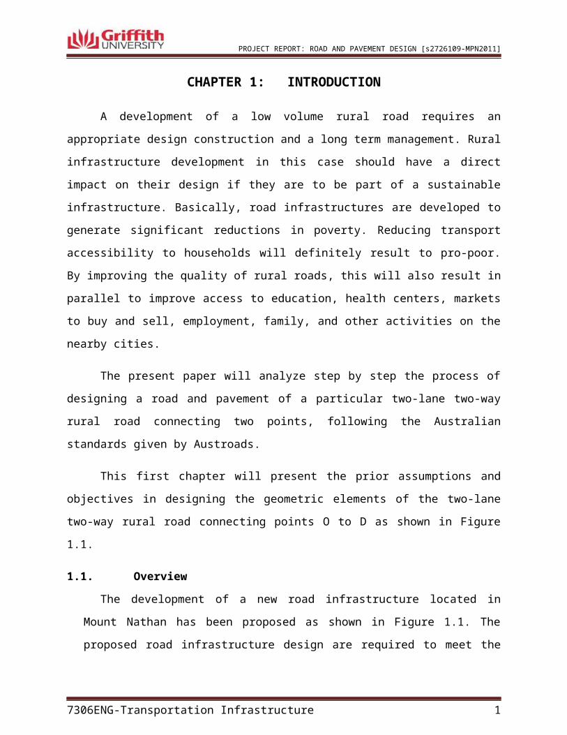
The development of a new road infrastructure located in Mount Nathan has been
proposed as shown in Figure 1.1. The proposed road infrastructure design are required to
meet the standard requirements in relevant to considering safety, amenity, convenience,
economy and sustainability. The design geometry of the road also should satisfy in terms of
its route location, horizontal and vertical alignments, cross-sectional elements and
earthworks.
7306ENG-Transportation Infrastructure 1
PROJECT REPORT: ROAD AND PAVEMENT DESIGN [s2726109-MPN2011]
Figure 1.1 Proposed developments detailing geographical location
1.2. Design Assumptions and Constraints
Design period= 20 years
Present year AADT = 4000 vehicles/day
Percentage of heavy vehicles = 10%
Compound growth factor =1.2%
Sub-grade CBR = 5%
Design speed= 80km/hr
K-factor = 15%
Directional distribution: 50/50
Maximum grade = 7% (rolling terrain)
Maximum height of the fill: 2.5m
Maximum height of cut: 3.0m
The following design was analyzed using 12d Model 9 road design software. The terrain
and contours were given in an electronic topographic map (Figure 2.2), as well as, the starting
point O (5263340.648, 6904871.943, 80) and end point D (525962.510, 6906996.263, 38).
7306ENG-Transportation Infrastructure 2
PROJECT REPORT: ROAD AND PAVEMENT DESIGN [s2726109-MPN2011]
CHAPTER 2: ROAD DESIGN
2.1. Overview
This second chapter will present the process of designing the geometric elements of the
two-lane two-way rural road connecting points O to D (see Figure 2.1). This involves evaluation
of route location, traverse layout (tangents and curves), horizontal alignment (curves,
superelevation, sight distances), vertical alignment (grades, curves, sight distances), Cross-
sectional elements (lanes, shoulders, drains) at 50m interval, earthworks and mass-haul diagram
using 12d Model 9 Software in junction with elementary analysis on cut and fill volume
calculations.
2.2. Design Input Parameters
2.2.1. Roadway Location
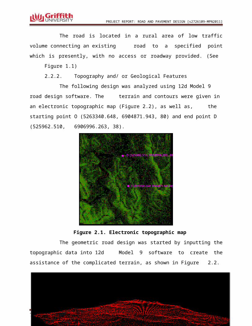
The road is located in a rural area of low traffic volume connecting an existing
road to a specified point which is presently, with no access or roadway provided. (See
Figure 1.1)
2.2.2. Topography and/ or Geological Features
The following design was analyzed using 12d Model 9 road design software. The
terrain and contours were given in an electronic topographic map (Figure 2.2), as well as,
the starting point O (5263340.648, 6904871.943, 80) and end point D (525962.510,
6906996.263, 38).
Figure 2.1. Electronic topographic map
7306ENG-Transportation Infrastructure 3
PROJECT REPORT: ROAD AND PAVEMENT DESIGN [s2726109-MPN2011]
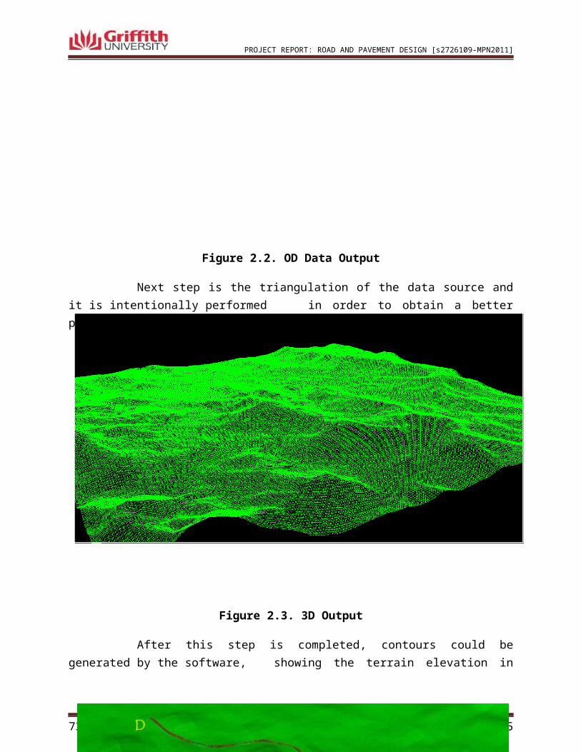
The geometric road design was started by inputting the topographic data into 12d
Model 9 software to create the assistance of the complicated terrain, as shown in Figure
2.2.
Figure 2.2. OD Data Output
Next step is the triangulation of the data source and it is intentionally performed in order to obtain a better perspective view of the topography.
Figure 2.3. 3D Output
7306ENG-Transportation Infrastructure 4
PROJECT REPORT: ROAD AND PAVEMENT DESIGN [s2726109-MPN2011]
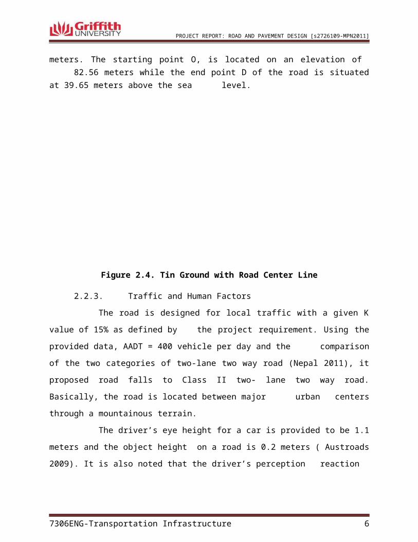
After this step is completed, contours could be generated by the software, showing the terrain elevation in meters. The starting point O, is located on an elevation of 82.56 meters while the end point D of the road is situated at 39.65 meters above the sea level.
Figure 2.4. Tin Ground with Road Center Line
2.2.3. Traffic and Human Factors
The road is designed for local traffic with a given K value of 15% as defined by
the project requirement. Using the provided data, AADT = 400 vehicle per day and the
comparison of the two categories of two-lane two way road (Nepal 2011), it proposed
road falls to Class II two- lane two way road. Basically, the road is located between major
urban centers through a mountainous terrain.
The driver’s eye height for a car is provided to be 1.1 meters and the object height
on a road is 0.2 meters ( Austroads 2009). It is also noted that the driver’s perception
reaction time varies from 1 to 3.6 seconds and in this design analysis, reaction time of 2.5
seconds be used as a desirable value.
2.2.4. Speed Parameters
Road traffic is a complex system in which several components interact
simultaneously. For a sustainable transportation system, it has to cater safety, convenient,
comfortable, secured, continuous, system coherency and attractive road design. But of all,
the most important requirement for a new road design is the selection of the appropriate
7306ENG-Transportation Infrastructure 5
PROJECT REPORT: ROAD AND PAVEMENT DESIGN [s2726109-MPN2011]
operating speed. This design speed was a analyzed in a iterative approach, which is
directly influenced by road design parameters including sight distance, horizontal curve
radii and topography. Standard parameters and sample computation as provided below
shows how reliable the analysis is.
R= v2
¿¿
where:
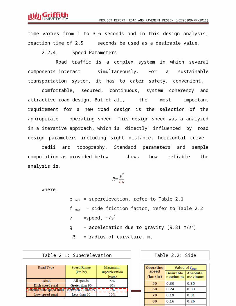
e max = superelevation, refer to Table 2.1
f max = side friction factor, refer to Table 2.2
v =speed, m/s2
g = acceleration due to gravity (9.81 m/s2)
R = radius of curvature, m.
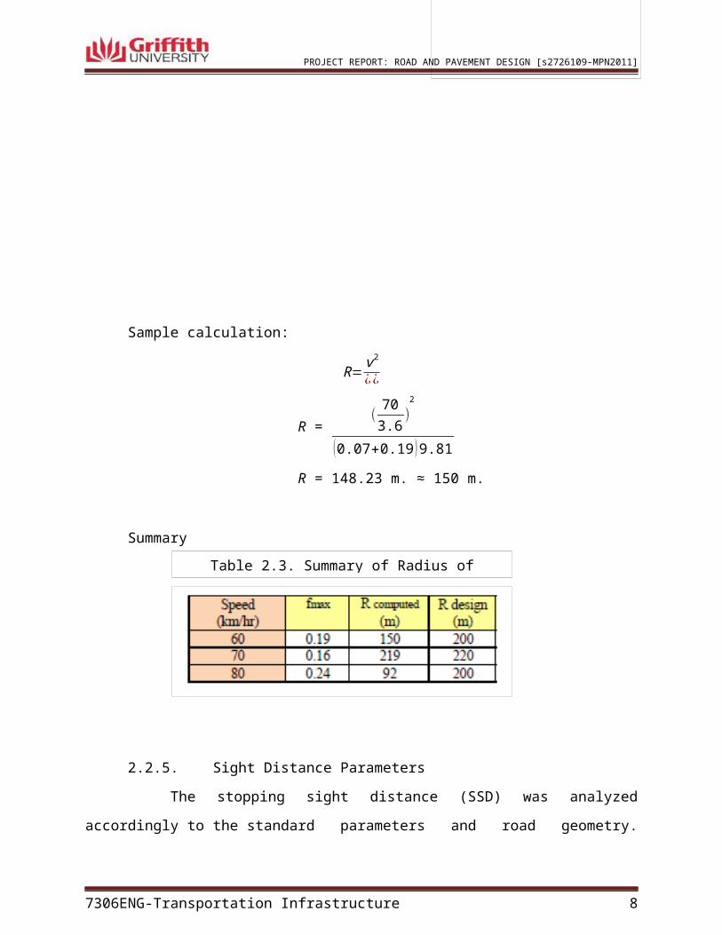
Sample calculation:
R= v2
¿¿
R = ( 703.6
)2
(0.07+0.19 )9.81
R = 148.23 m. ≈ 150 m.
7306ENG-Transportation Infrastructure 6
Table 2.2: Side Friction FactorTable 2.1: Superelevation
PROJECT REPORT: ROAD AND PAVEMENT DESIGN [s2726109-MPN2011]
Summary
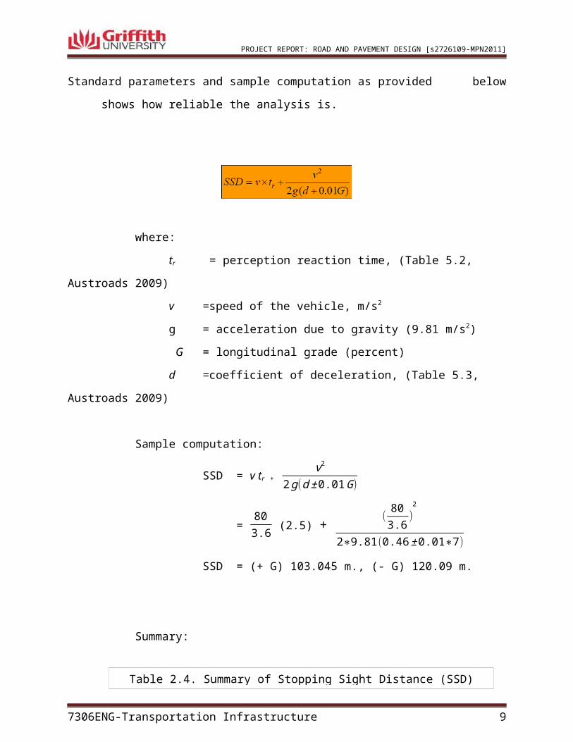
2.2.5. Sight Distance Parameters
The stopping sight distance (SSD) was analyzed accordingly to the standard
parameters and road geometry. Standard parameters and sample computation as provided
below shows how reliable the analysis is.
where:
tr = perception reaction time, (Table 5.2, Austroads 2009)
v =speed of the vehicle, m/s2
g = acceleration due to gravity (9.81 m/s2)
G = longitudinal grade (percent)
d =coefficient of deceleration, (Table 5.3, Austroads 2009)
Sample computation:
SSD = v tr + v2
2 g(d± 0.01 G)
= 803.6 (2.5) +
( 803.6
)2
2∗9.81(0.46 ± 0.01∗7)
SSD = (+ G) 103.045 m., (- G) 120.09 m.
7306ENG-Transportation Infrastructure 7
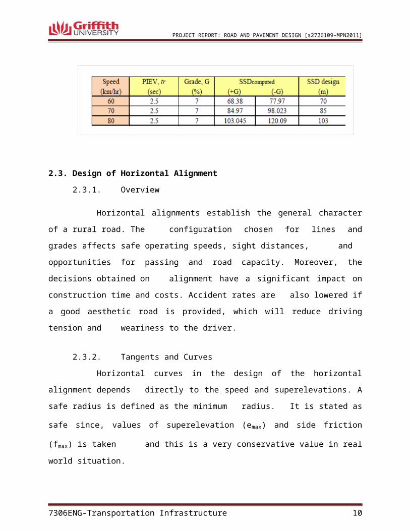
Table 2.3. Summary of Radius of Curvature
PROJECT REPORT: ROAD AND PAVEMENT DESIGN [s2726109-MPN2011]
Summary:
2.3. Design of Horizontal Alignment
2.3.1. Overview
Horizontal alignments establish the general character of a rural road. The
configuration chosen for lines and grades affects safe operating speeds, sight distances,
and opportunities for passing and road capacity. Moreover, the decisions obtained on
alignment have a significant impact on construction time and costs. Accident rates are
also lowered if a good aesthetic road is provided, which will reduce driving tension and
weariness to the driver.
2.3.2. Tangents and Curves
Horizontal curves in the design of the horizontal alignment depends
directly to the speed and superelevations. A safe radius is defined as the minimum radius.
It is stated as safe since, values of superelevation (emax) and side friction (fmax) is taken
and this is a very conservative value in real world situation.
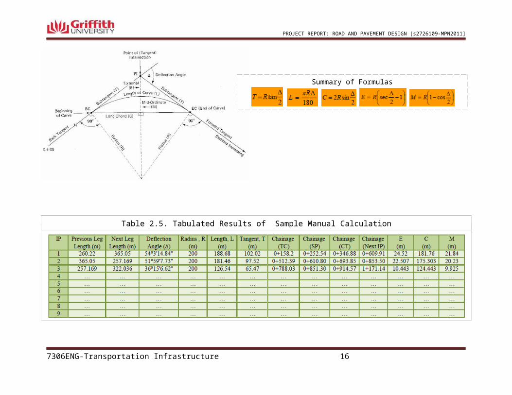
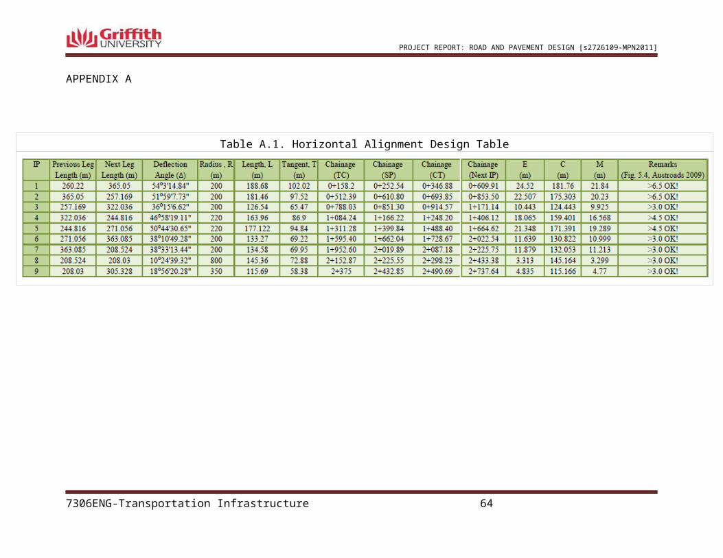
After series of iterations, the final geometry results to a total of nine
horizontal curves. The relevant horizontal alignment parameters are presented in
Appendix A, Table A.1 . The smallest radii used is 200 m. which satisfies the minimum
requirement of 92 m.
7306ENG-Transportation Infrastructure 8
Table 2.4. Summary of Stopping Sight Distance (SSD)
PROJECT REPORT: ROAD AND PAVEMENT DESIGN [s2726109-MPN2011]
7306ENG-Transportation Infrastructure 9
PROJECT REPORT: ROAD AND PAVEMENT DESIGN [s2726109-MPN2011]
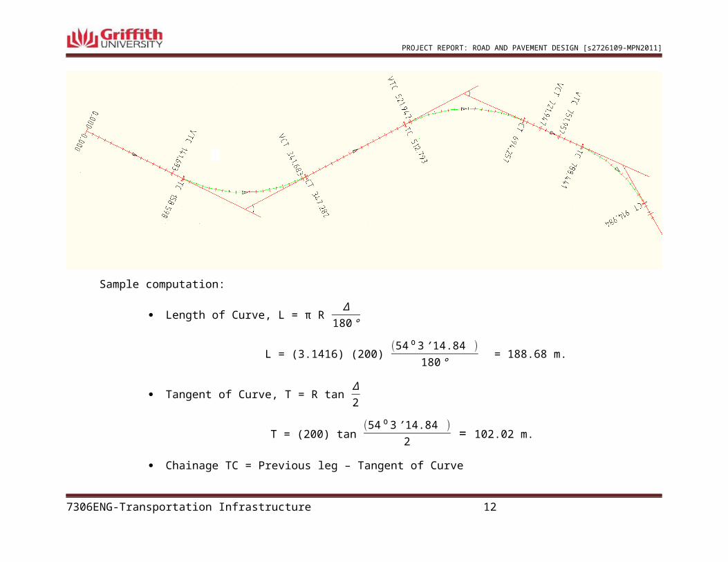
Sample computation:
Length of Curve, L = π R ∆
180°
L = (3.1416) (200) (54 ⁰3 ’14.84 ”)
180 ° = 188.68 m.
Tangent of Curve, T = R tan ∆2
T = (200) tan (54 ⁰3 ’14.84 ”)
2 = 102.02 m.
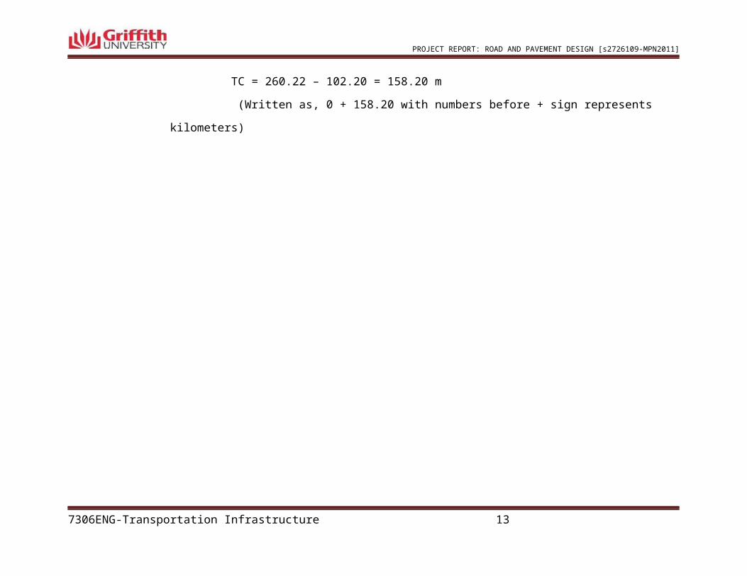
Chainage TC = Previous leg – Tangent of Curve
TC = 260.22 – 102.20 = 158.20 m
(Written as, 0 + 158.20 with numbers before + sign represents kilometers)
7306ENG-Transportation Infrastructure 10
PROJECT REPORT: ROAD AND PAVEMENT DESIGN [s2726109-MPN2011]
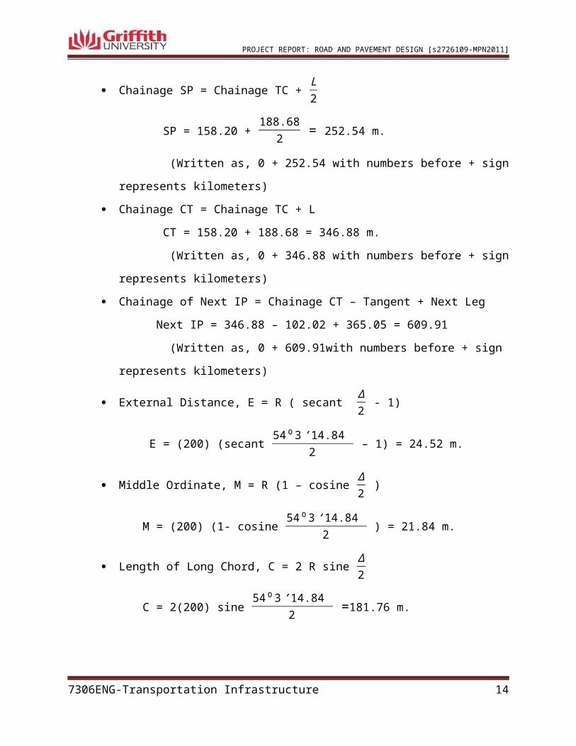
Chainage SP = Chainage TC + L2
SP = 158.20 + 188.68
2 = 252.54 m.
(Written as, 0 + 252.54 with numbers before + sign represents kilometers)
Chainage CT = Chainage TC + L
CT = 158.20 + 188.68 = 346.88 m.
(Written as, 0 + 346.88 with numbers before + sign represents kilometers)
Chainage of Next IP = Chainage CT – Tangent + Next Leg
Next IP = 346.88 – 102.02 + 365.05 = 609.91
(Written as, 0 + 609.91with numbers before + sign represents kilometers)
External Distance, E = R ( secant ∆2
- 1)
E = (200) (secant 54 ⁰ 3’ 14.84 ”
2 – 1) = 24.52 m.
Middle Ordinate, M = R (1 – cosine ∆2
)
M = (200) (1- cosine 54 ⁰ 3’ 14.84 ”
2 ) = 21.84 m.
Length of Long Chord, C = 2 R sine ∆2
C = 2(200) sine 54 ⁰ 3’ 14.84 ”
2 =181.76 m.
7306ENG-Transportation Infrastructure 11
PROJECT REPORT: ROAD AND PAVEMENT DESIGN [s2726109-MPN2011]
Refer to appendix A. Table A.1 for full tabulation of the manual calculation of tangents and curves.
7306ENG-Transportation Infrastructure 12
Table 2.5. Tabulated Results of Sample Manual Calculation
Summary of Formulas
PROJECT REPORT: ROAD AND PAVEMENT DESIGN [s2726109-MPN2011]
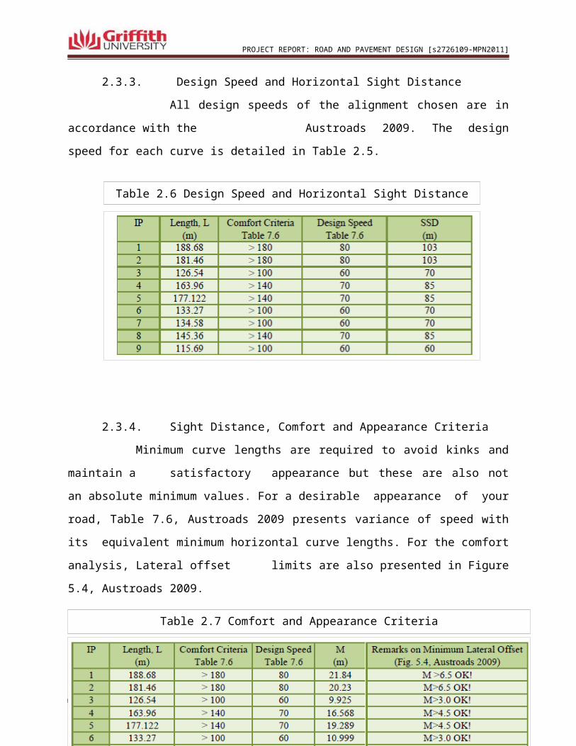
2.3.3. Design Speed and Horizontal Sight Distance
All design speeds of the alignment chosen are in accordance with the
Austroads 2009. The design speed for each curve is detailed in Table 2.5.
2.3.4. Sight Distance, Comfort and Appearance Criteria
Minimum curve lengths are required to avoid kinks and maintain a satisfactory
appearance but these are also not an absolute minimum values. For a desirable
appearance of your road, Table 7.6, Austroads 2009 presents variance of speed with its
equivalent minimum horizontal curve lengths. For the comfort analysis, Lateral offset
limits are also presented in Figure 5.4, Austroads 2009.
7306ENG-Transportation Infrastructure 13
Table 2.6 Design Speed and Horizontal Sight Distance
Table 2.7 Comfort and Appearance Criteria
PROJECT REPORT: ROAD AND PAVEMENT DESIGN [s2726109-MPN2011]
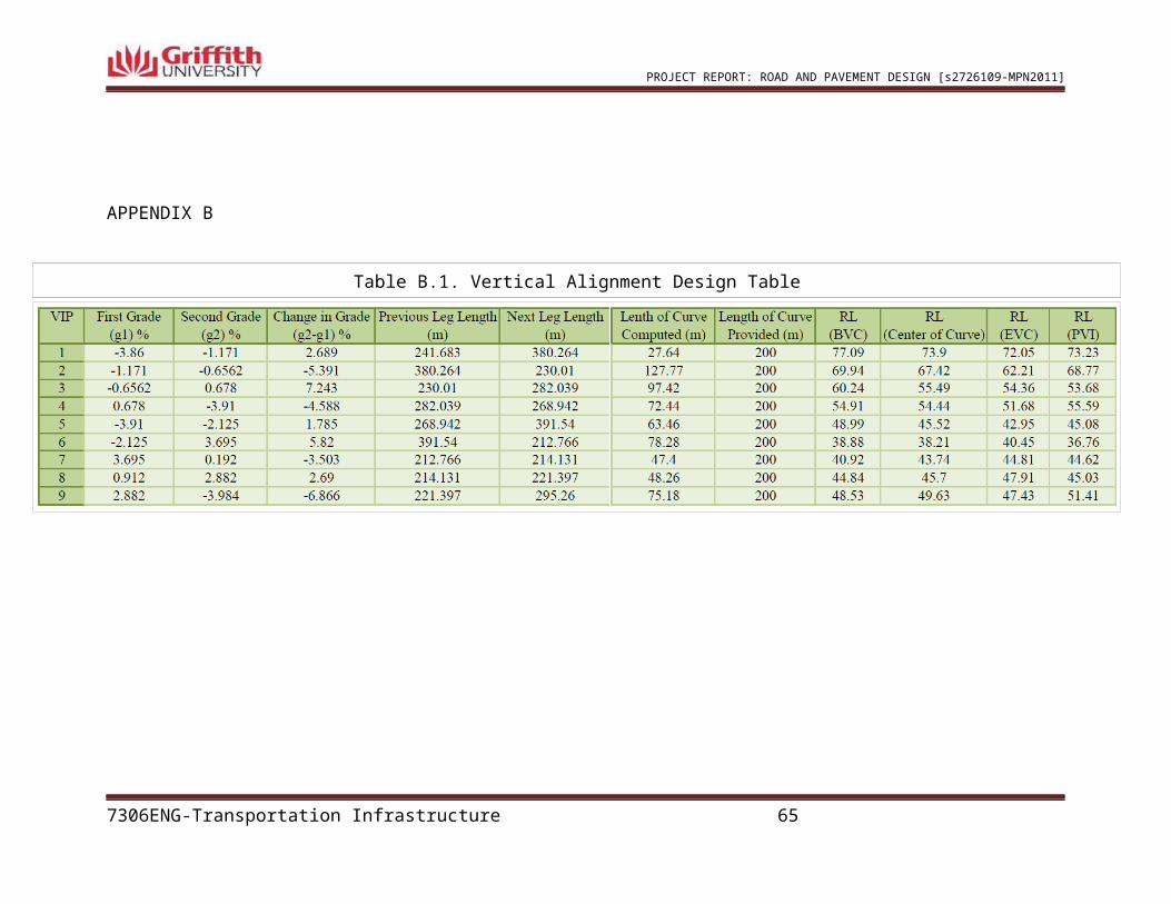
2.4. Design of Vertical Alignment
2.4.1. Overview
Vertical elements should be superimposed on horizontal ones in such a way that
the intersection points practically coincide with the horizontal slightly in advance to the
vertical and horizontal and vertical curves of similar lengths. (Nepal 2011) The design
speed of the road in both planes are taken to be the same. In this case, it will give a hand
on the driver’s awareness of the speed environment.
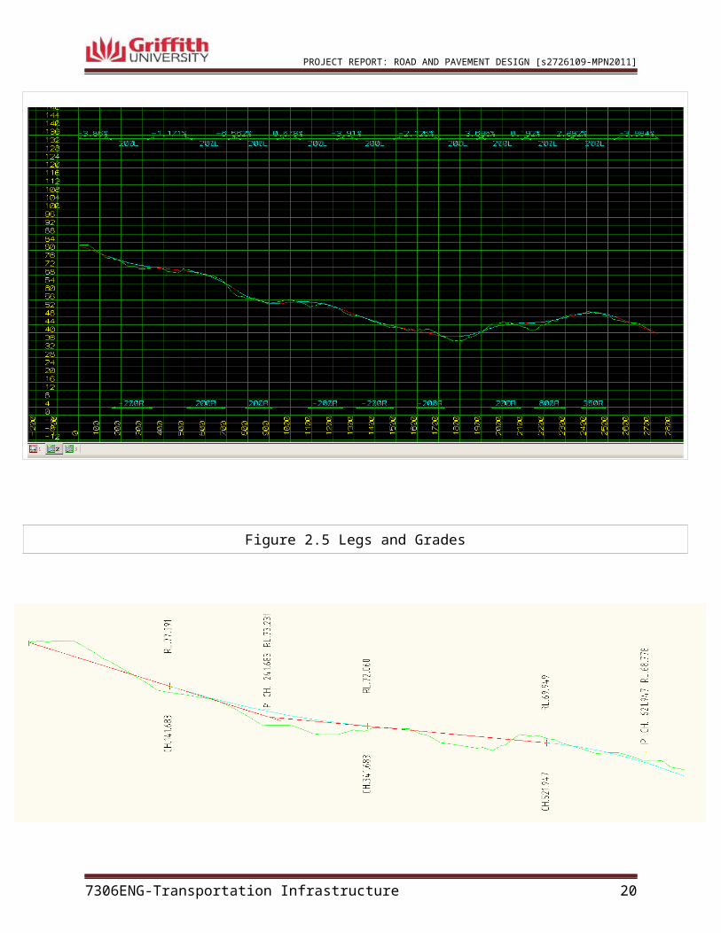
2.4.2. Legs and Grades
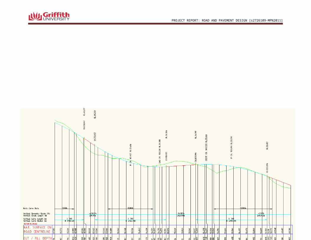
Basically, as much as possible the grade of the road should follow the natural
contours, however, for the chosen road geometry, the minimum grade obtain is 0.192%.
On the other hand, the maximum grade of this alignment is 3.984%, which fall under 7%
absolute maximum grade or 5% desirable maximum grade and 0.3% absolute minimum
grade or 0.1% desirable minimum grade. (GCCC, 2005). Detailed plots are shown in
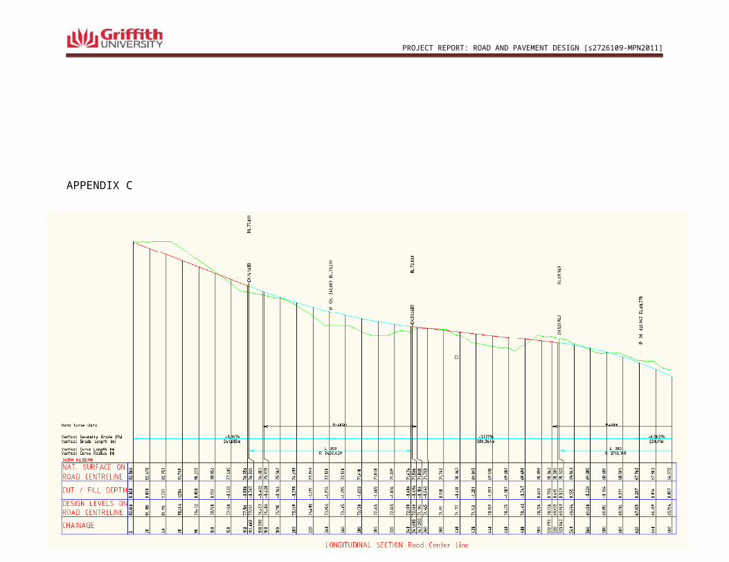
Appendix C.
7306ENG-Transportation Infrastructure 14
Figure 2.5 Legs and Grades

PROJECT REPORT: ROAD AND PAVEMENT DESIGN [s2726109-MPN2011]
2.4.3. Sight Distance, Comfort and Appearance Criteria
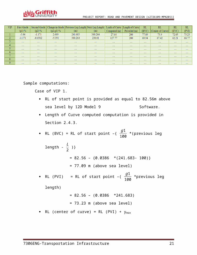
Sample computations:
Case of VIP 1.
RL of start point is provided as equal to 82.56m above sea level by 12D Model 9
Software.
Length of Curve computed computation is provided in Section 2.4.3.
RL (BVC) = RL of start point –{ g 1100
*(previous leg length - L2
)}
= 82.56 – {0.0386 *(241.683- 100)}
= 77.09 m (above sea level)
RL (PVI) = RL of start point –( g 1100
*previous leg length)
= 82.56 – (0.0386 *241.683)
= 73.23 m (above sea level)
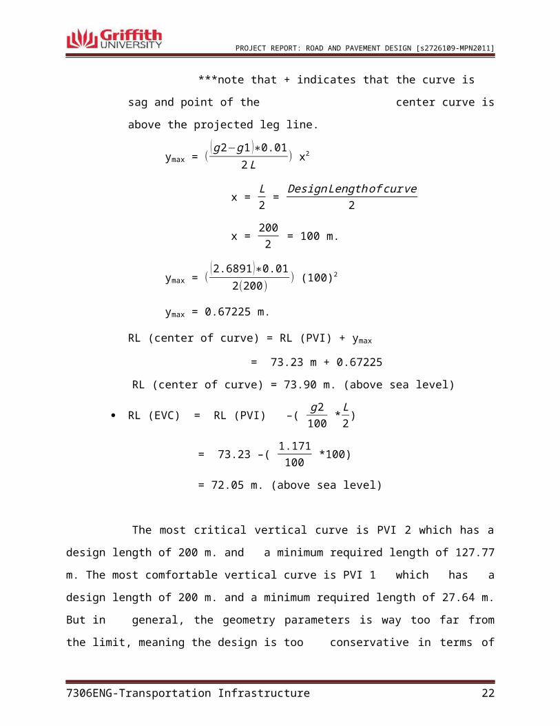
RL (center of curve) = RL (PVI) + ymax
7306ENG-Transportation Infrastructure 15
PROJECT REPORT: ROAD AND PAVEMENT DESIGN [s2726109-MPN2011]
***note that + indicates that the curve is sag and point of the
center curve is above the projected leg line.
ymax = ((g2−g1 )∗0.01
2L) x2
x = L2
= Design Lengthof cur ve
2
x = 200
2 = 100 m.
ymax = ((2.6891 )∗0.01
2(200)) (100)2
ymax = 0.67225 m.
RL (center of curve) = RL (PVI) + ymax
= 73.23 m + 0.67225
RL (center of curve) = 73.90 m. (above sea level)
RL (EVC) = RL (PVI) –( g 2100
*L2
)
= 73.23 –( 1.171100
*100)
= 72.05 m. (above sea level)
The most critical vertical curve is PVI 2 which has a design length of 200 m. and
a minimum required length of 127.77 m. The most comfortable vertical curve is PVI 1
which has a design length of 200 m. and a minimum required length of 27.64 m. But in
general, the geometry parameters is way too far from the limit, meaning the design is too
conservative in terms of comfort. Refer to appendix B. Table B.1 for full tabulation of the
calculation
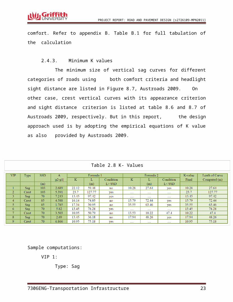
2.4.3. Minimum K values
The minimum size of vertical sag curves for different categories of roads using
both comfort criteria and headlight sight distance are listed in Figure 8.7, Austroads 2009.
On other case, crest vertical curves with its appearance criterion and sight distance
criterion is listed at table 8.6 and 8.7 of Austroads 2009, respectively. But in this report,
7306ENG-Transportation Infrastructure 16
PROJECT REPORT: ROAD AND PAVEMENT DESIGN [s2726109-MPN2011]
the design approach used is by adopting the empirical equations of K value as also
provided by Austroads 2009.
Sample computations:
VIP 1:
Type: Sag
SSD = SD = 103 m.
Using Austroads 2009 formulas for sag vertical curves:
Case 1:
= 1032
200¿¿ = 22.12
A = |g2 – g1| = 2.689
L = K A = (22.12)(2.689) = 59.48 m. ; L < SD, then it doesn’t satisfy!
Case 2:
7306ENG-Transportation Infrastructure 17
Table 2.8 K- Values
L > SD
L < SD
SD = Sight Distanceh1 = observer’s height (1.1m)h2 = objects height (0.2m)h = mounting height of headlights (0.6m)V = speed (km/h)θ = elevation angle of beam (1º)g1 = grade previous legg1 = grade next legL =K AA = |g2 – g1|
K=( SD )2
200 (h+SD tanθ )
K= 2×SD|g2−g1|
−200 (h+SD tan θ)
(|g2−g1|)2
K=( SD )2
200 (h+SD tanθ )
K= 2×SD|g2−g1|
−200 (h+SD tan θ)
(|g2−g1|)2
PROJECT REPORT: ROAD AND PAVEMENT DESIGN [s2726109-MPN2011]
= 2(103)2.689
– 200¿¿ = 10.28
L = K A = (10.98) (2.689) = 27.64 m.; L < SD, ok!
2.5. Design of Cross Sections
2.5.1. Overview
The dimension of a typical; cross section is based on parameters such as traffic
volume dimensions and combination of speed and traffic volume. (Austroads 2009)
2.5.2. Elements of Cross Sections
The whole length of the road design is considered to have a fixed cross section
lane width of 3.2 m, shoulder width of 1.2 m and the drainage details is taken as to be the
minimum design since, it is not included in the overall design analysis of the road design
project. The cross fall and superelevation slope of the road and shoulder varies
accordingly as chainage changes. This is due to the main purpose of the design which is,
to accommodate both cars and trucks for the design speed of the road.
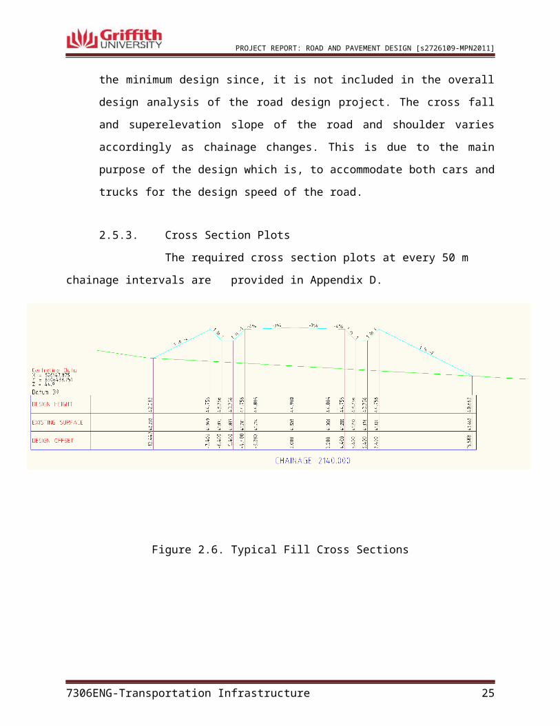
2.5.3. Cross Section Plots
The required cross section plots at every 50 m chainage intervals are
provided in Appendix D.
Figure 2.6. Typical Fill Cross Sections
7306ENG-Transportation Infrastructure 18
PROJECT REPORT: ROAD AND PAVEMENT DESIGN [s2726109-MPN2011]
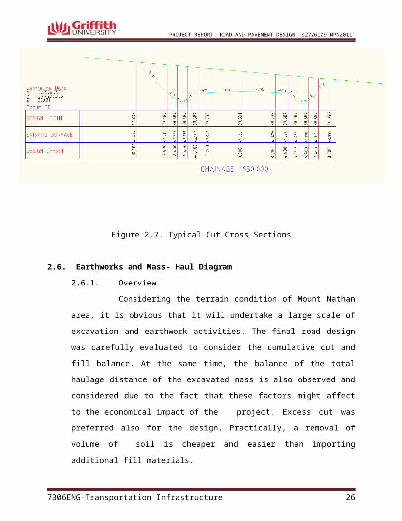
Figure 2.7. Typical Cut Cross Sections
2.6. Earthworks and Mass- Haul Diagram
2.6.1. Overview
Considering the terrain condition of Mount Nathan area, it is obvious that
it will undertake a large scale of excavation and earthwork activities. The final road
design was carefully evaluated to consider the cumulative cut and fill balance. At the
same time, the balance of the total haulage distance of the excavated mass is also
observed and considered due to the fact that these factors might affect to the economical
impact of the project. Excess cut was preferred also for the design. Practically, a
removal of volume of soil is cheaper and easier than importing additional fill materials.
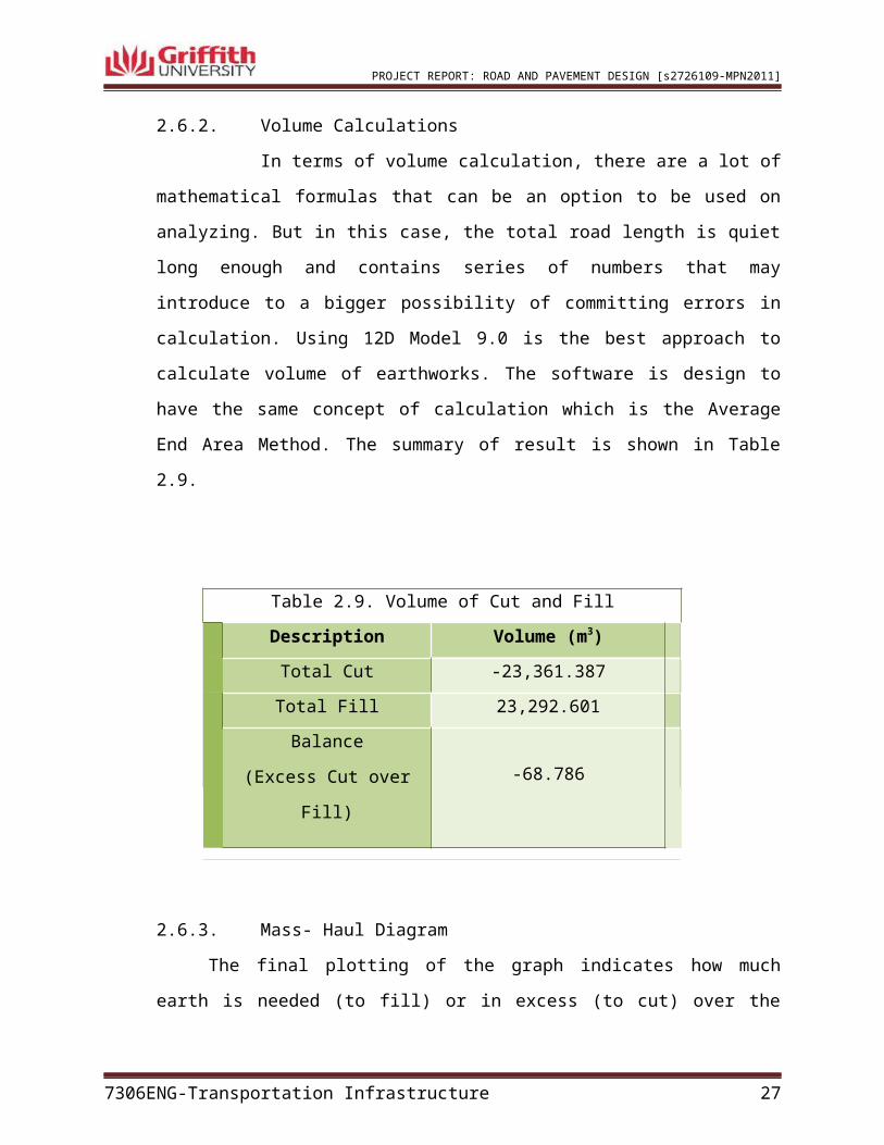
2.6.2. Volume Calculations
In terms of volume calculation, there are a lot of mathematical formulas
that can be an option to be used on analyzing. But in this case, the total road length is
quiet long enough and contains series of numbers that may introduce to a bigger
possibility of committing errors in calculation. Using 12D Model 9.0 is the best approach
7306ENG-Transportation Infrastructure 19
PROJECT REPORT: ROAD AND PAVEMENT DESIGN [s2726109-MPN2011]
to calculate volume of earthworks. The software is design to have the same concept of
calculation which is the Average End Area Method. The summary of result is shown in
Table 2.9.
Table 2.9. Volume of Cut and Fill
Description Volume (m3)
Total Cut -23,361.387
Total Fill 23,292.601
Balance
(Excess Cut over Fill) -68.786
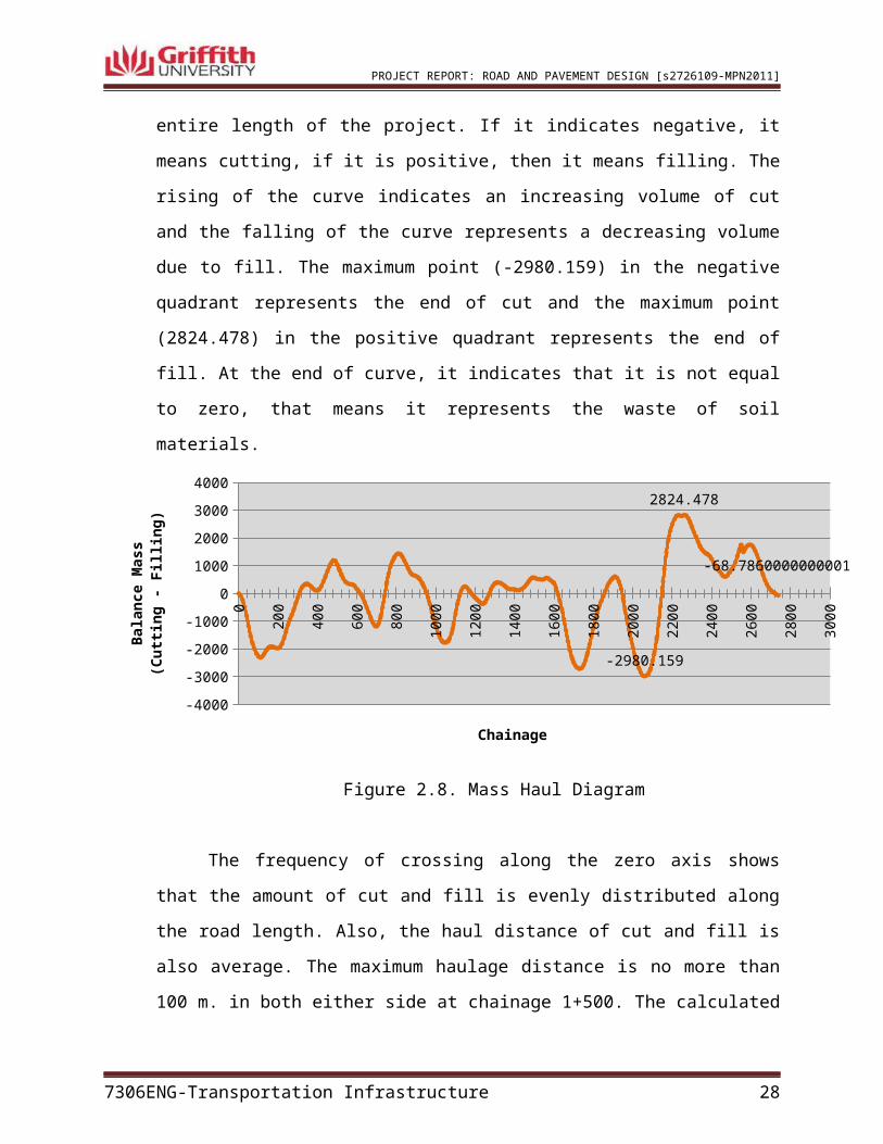
2.6.3. Mass- Haul Diagram
The final plotting of the graph indicates how much earth is needed (to fill) or in
excess (to cut) over the entire length of the project. If it indicates negative, it means
cutting, if it is positive, then it means filling. The rising of the curve indicates an
increasing volume of cut and the falling of the curve represents a decreasing volume due
to fill. The maximum point (-2980.159) in the negative quadrant represents the end of cut
and the maximum point (2824.478) in the positive quadrant represents the end of fill. At
the end of curve, it indicates that it is not equal to zero, that means it represents the waste
of soil materials.
7306ENG-Transportation Infrastructure 20
PROJECT REPORT: ROAD AND PAVEMENT DESIGN [s2726109-MPN2011]
0
200
400
600
800
1000
1200
1400
1600
1800
2000
2200
2400
2600
2800
3000
-4000
-3000
-2000
-1000
0
1000
2000
3000
4000
-2980.159
2824.478
-68.7860000000001
Chainage
Bala
nce
Mas
s(C
utting
- Fi
lling
)
Figure 2.8. Mass Haul Diagram
The frequency of crossing along the zero axis shows that the amount of cut and
fill is evenly distributed along the road length. Also, the haul distance of cut and fill is
also average. The maximum haulage distance is no more than 100 m. in both either side
at chainage 1+500. The calculated final cut-fill balance of the road design was calculated
to be -68.786 m3, which is satisfying the maximum required of 10% of the total fill
volume.
The volume calculated represents an excess on cutting activity which in fact, there
is no need for the contractor to look for an imported fill. In this way, the desired
economical prospective is achieved.
7306ENG-Transportation Infrastructure 21
PROJECT REPORT: ROAD AND PAVEMENT DESIGN [s2726109-MPN2011]
CHAPTER 3: PAVEMENT DESIGN
3.1. Overview
Produce alternative flexible pavement designs for the same two-lane two-way rural road. The alternative design includes:
(a) Granular pavement with asphalt wearing surface(b) Asphalt surfaced pavement with cemented base(c) Full depth asphalt (d) Asphalt, granular base and cemented sub-base
3.2. Design Input Parameters
Design period = 20 yearsPresent year AADT = 4000 vehicles.Percentage of heavy vehicles= 10% vehicles. (Compound growth factor = 1.2%)Sub-grade CBR = 5%Design speed = 80km/hrK-factor = 15 %Directional distribution: 50/50Maximum grade = 7% (rolling terrain)Maximum height of the fill: 2.5mMaximum height of the cut: 3.0mTerrain and contours are shown in topographic map in Figure 1.2 and 2.1.Determination of lane distribution factor (LDF) = 1.0,
7306ENG-Transportation Infrastructure 22
PROJECT REPORT: ROAD AND PAVEMENT DESIGN [s2726109-MPN2011]
***refer to Appendix E.Table 7.3,Austroads,2010.Determination of cumulative growth factor (CGF) = 22.46
*** refer to Appendix E. Table 7.4., Austroads,2010NHVAG value can be obtain from Table F2, Austroads 2010, Presumptive traffic load distribution for rural road.Project Reliabilty = 90% , refer to Appendix E. Table 2.1
Cumulative HVAG = 365 x (AADT x DF) x HV x NHVAG x LDF x CGF = 365 x (4000 x 0.50) x 0.10 x 2.8 x 1.0 x 22.46
HVAG = 4.59 x 10 6
Establish the traffic load distribution (TLD):
Design SAR (DSAR):
Design ESA or DESA = ESA
HVAG x HVAG = 0.90 (4.59 x 10⁶) = 4.131 x 10⁶
DSAR5 = DESA x 1.1 = 4.5441 x 10 6
DSAR7 = DESA x 1.1 = 6.6096 x 10 6
DSAR12 = DESA x 1.1 = 4.957 x 10 6
3.3. Flexible Pavement Design
3.3.1. Granular Pavement with Asphalt Wearing Surface
Using Chart EC02:
The design approach of this type of Flexible Pavement Design was
carefully analyzed by using design charts, for a sub-grade Modulus of 50
MPa and DESA = 4.131 x 10⁶ the appropriate chart is chart 2 (EC02).
(Austroads, 2010)
7306ENG-Transportation Infrastructure 23

CBR 5 Subgrade
CBR 5 Subgrade
PROJECT REPORT: ROAD AND PAVEMENT DESIGN [s2726109-MPN2011]
Thickness Superior Edge Selected Inferior Edge
Asphalt (mm) 205 180 170
Unbound Granular Material (mm)
100 350 500
Using CIRCLY 5.0 Software:
1. Trial Pavement
7306ENG-Transportation Infrastructure 24
350 mm Granular base
180 mm Asphalt
180 mm Asphalt
PROJECT REPORT: ROAD AND PAVEMENT DESIGN [s2726109-MPN2011]
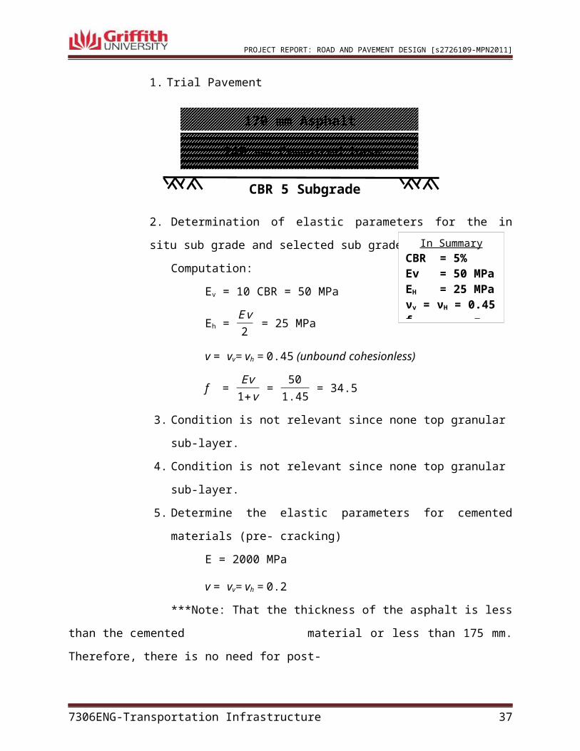
2. Determination of elastic parameters for the in situ sub grade and selected
sub grade materials:
Computation:
Ev = 10 CBR = 50 MPa
Eh = E v2
= 25 MPa
v = vv= vh = 0.45 (unbound cohesionless)
f = Ev
1+v =
501.45
= 34.5
3. Condition is not relevant since none top granular sub-layer.
4. Condition is not relevant since none top granular sub-layer.
5. Not relevant.
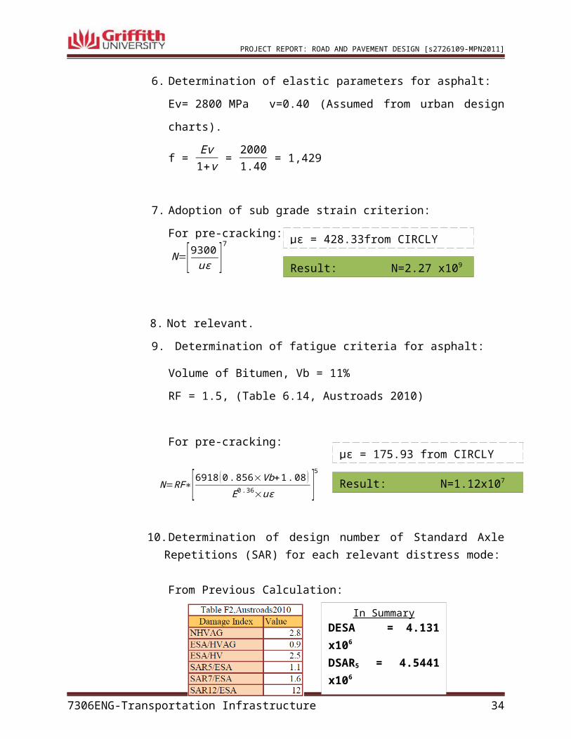
6. Determination of elastic parameters for asphalt:
Ev= 2800 MPa v=0.40 (Assumed from urban design charts).
f = Ev
1+v =
20001.40
= 1,429
7. Adoption of sub grade strain criterion:
For pre-cracking:
8. Not relevant.
9. Determination of fatigue criteria for asphalt:
7306ENG-Transportation Infrastructure 25
με = 428.33from CIRCLY (Figure 3.1 )Result: N=2.27 x10⁹
In SummaryCBR = 5%Ev = 50 MPaEH = 25 MPaνv = νH = 0.45f = 34.5
350 mm Granular base
N=[9300uε ]
7
PROJECT REPORT: ROAD AND PAVEMENT DESIGN [s2726109-MPN2011]
Volume of Bitumen, Vb = 11%
RF = 1.5, (Table 6.14, Austroads 2010)
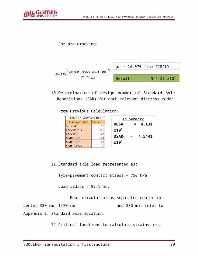
For pre-cracking:
10. Determination of design number of Standard Axle Repetitions (SAR) for each relevant distress mode:
From Previous Calculation:
11. Standard axle load represented as:
Tyre-pavement contact stress = 750 kPa
Load radius = 92.1 mm.
Four circular areas separated center-to-center 330 mm, 1470 mm
and 330 mm, refer to Appendix E. Standard axle location.
12. Critical locations to calculate strains are:
Top of sub-grade
Bottom of asphalt later
Bottom of cemented layer
13. CIRCLY output
7306ENG-Transportation Infrastructure 26
με = 175.93 from CIRCLY (Figure 3.1 )Result: N=1.12x10⁷
In SummaryDESA = 4.131 x10⁶
DSAR5 = 4.5441 x10⁶
DSAR7 = 6.6096 x10⁶
DSAR12 = 4.957 x10⁷
N=RF∗[6918 (0. 856×Vb+1 .08 )E0 .36×uε ]
5
PROJECT REPORT: ROAD AND PAVEMENT DESIGN [s2726109-MPN2011]
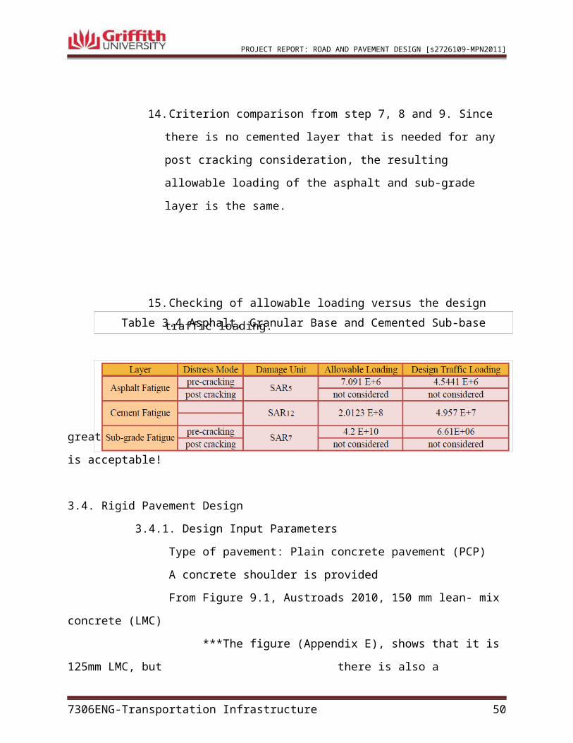
14. Criterion comparison from step 7, 8 and 9. It is noted that the post-
cracking of the cemented material is not considered. The resulting
allowable loading is the same.
15. Checking of allowable loading versus the design traffic loading.
16. Remarks.
Since allowable loading of all layers is greater than design traffic
loading, the design is acceptable!
7306ENG-Transportation Infrastructure 27
Figure 3.1. Granular Pavement with Asphalt Wearing Surface (CIRCLY 5.0 result)
Table 3.1 Granular Pavement with Asphalt Wearing Surface
170 mm Asphalt
240 mm Cemented base
CBR 5 Subgrade
PROJECT REPORT: ROAD AND PAVEMENT DESIGN [s2726109-MPN2011]
3.3.2. Asphalt Surfaced Pavement with Cemented Base
1. Trial Pavement
2. Determination of elastic parameters for the in situ sub grade and selected
sub grade materials:
Computation:
Ev = 10 CBR = 50 MPa
Eh = E v2
= 25 MPa
v = vv= vh = 0.45 (unbound cohesionless)
f = Ev
1+v =
501.45
= 34.5
3. Condition is not relevant since none top granular sub-layer.
4. Condition is not relevant since none top granular sub-layer.
5. Determine the elastic parameters for cemented materials (pre- cracking)
E = 2000 MPa
v = vv= vh = 0.2
***Note: That the thickness of the asphalt is less than the cemented
material or less than 175 mm. Therefore, there is no need for post-
cracking analysis. (Austroads,2010)
6. Determination of elastic parameters for asphalt:
Ev= 2000 MPa v=0.40 (Assumed from urban design charts).
f = Ev
1+v =
20001.40
= 1,429
7. Adoption of sub grade strain criterion:
7306ENG-Transportation Infrastructure 28
In SummaryCBR = 5%Ev = 50 MPaEH = 25 MPaνv = νH = 0.45f = 34.5
PROJECT REPORT: ROAD AND PAVEMENT DESIGN [s2726109-MPN2011]
For pre-cracking:
8. Determination of fatigue criteria for cemented materials
Project Reliability = 90 %
RF = 2.0 (Table 6.8, Austroads 2010)
9. Determination of fatigue criteria for asphalt:
Volume of Bitumen, Vb = 11%
RF = 1.5, (Table 6.14, Austroads 2010)
For pre-cracking:
10. Determination of design number of Standard Axle Repetitions (SAR) for each relevant distress mode:
From Previous Calculation:
7306ENG-Transportation Infrastructure 29
In SummaryDESA = 4.131 x10⁶
DSAR5 = 4.5441 x10⁶
DSAR7 = 6.6096 x10⁶
DSAR12 = 4.957 x10⁷
Result: N=4.28 x10¹¹
με = 24.075 from CIRCLY (Figure 3.2 )
Result: N=6.43 x10⁷
με = 7104.53 from CIRCLY (Figure 3.2 )
με = 247.31 from CIRCLY (Figure 3.2 )Result: N=81.06 x10¹¹N=[9300
uε ]7
N=RF [ (113000E0. 804 )+191
uε ]12
N=RF∗[6918 (0. 856×Vb+1 .08 )E0 .36×uε ]
5
PROJECT REPORT: ROAD AND PAVEMENT DESIGN [s2726109-MPN2011]
11. Standard axle load represented as:
Tyre-pavement contact stress = 750 kPa
Load radius = 92.1 mm.
Four circular areas separated center-to-center 330 mm, 1470 mm
and 330 mm, refer to Appendix E. Standard axle location.
12. Critical locations to calculate strains are:
Top of sub-grade
Bottom of asphalt later
Bottom of cemented layer
13. CIRCLY output
7306ENG-Transportation Infrastructure 30
PROJECT REPORT: ROAD AND PAVEMENT DESIGN [s2726109-MPN2011]
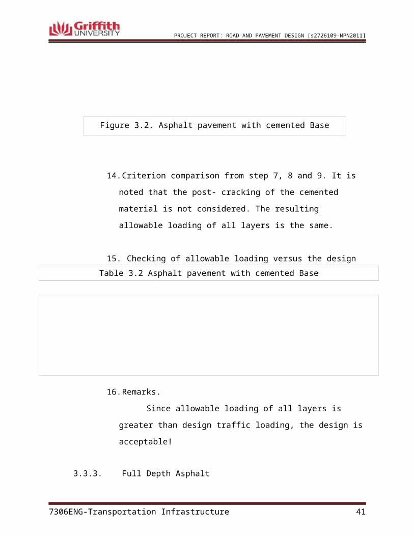
14. Criterion comparison from step 7, 8 and 9. It is noted that the post-
cracking of the cemented material is not considered. The resulting
allowable loading of all layers is the same.
15. Checking of allowable loading versus the design traffic loading.
16. Remarks.
Since allowable loading of all layers is greater than design traffic
loading, the design is acceptable!
3.3.3. Full Depth Asphalt
7306ENG-Transportation Infrastructure 31
Figure 3.2. Asphalt pavement with cemented Base (CIRCLY 5.0 result)
Table 3.2 Asphalt pavement with cemented Base
200 mm Asphalt
CBR 5 Subgrade
PROJECT REPORT: ROAD AND PAVEMENT DESIGN [s2726109-MPN2011]
1. Trial Pavement
2. Determination of elastic parameters for the in situ sub grade and selected
sub grade materials:
Computation:
Ev = 10 CBR = 50 MPa
Eh = E v2
= 25 MPa
v = vv= vh = 0.45 (unbound cohesionless)
f = Ev
1+v =
501.45
= 34.5
3. Condition is not relevant since none top granular sub-layer.
4. Condition is not relevant since none top granular sub-layer.
5. Condition is not relevant since there are no cemented material.
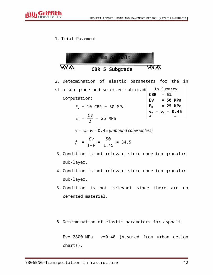
6. Determination of elastic parameters for asphalt:
Ev= 2800 MPa v=0.40 (Assumed from urban design charts).
f = Ev
1+v =
28001.40
= 2000
7. Adoption of sub grade strain criterion:
For pre-cracking:
8. Not relevant.
7306ENG-Transportation Infrastructure 32
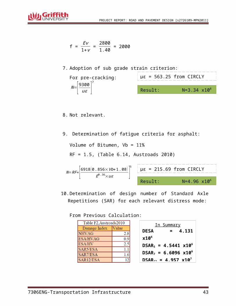
με = 563.25 from CIRCLY (Figure 3.4 )Result: N=3.34 x10⁸
In SummaryCBR = 5%Ev = 50 MPaEH = 25 MPaνv = νH = 0.45f = 34.5
N=[9300uε ]
7
PROJECT REPORT: ROAD AND PAVEMENT DESIGN [s2726109-MPN2011]
9. Determination of fatigue criteria for asphalt:
Volume of Bitumen, Vb = 11%
RF = 1.5, (Table 6.14, Austroads 2010)
10. Determination of design number of Standard Axle Repetitions (SAR) for each relevant distress mode:
From Previous Calculation:
11. Standard axle load represented as:
Tyre-pavement contact stress = 750 kPa
Load radius = 92.1 mm.
Four circular areas separated center-to-center 330 mm, 1470 mm and 330 mm, refer to Appendix E. Standard axle location.
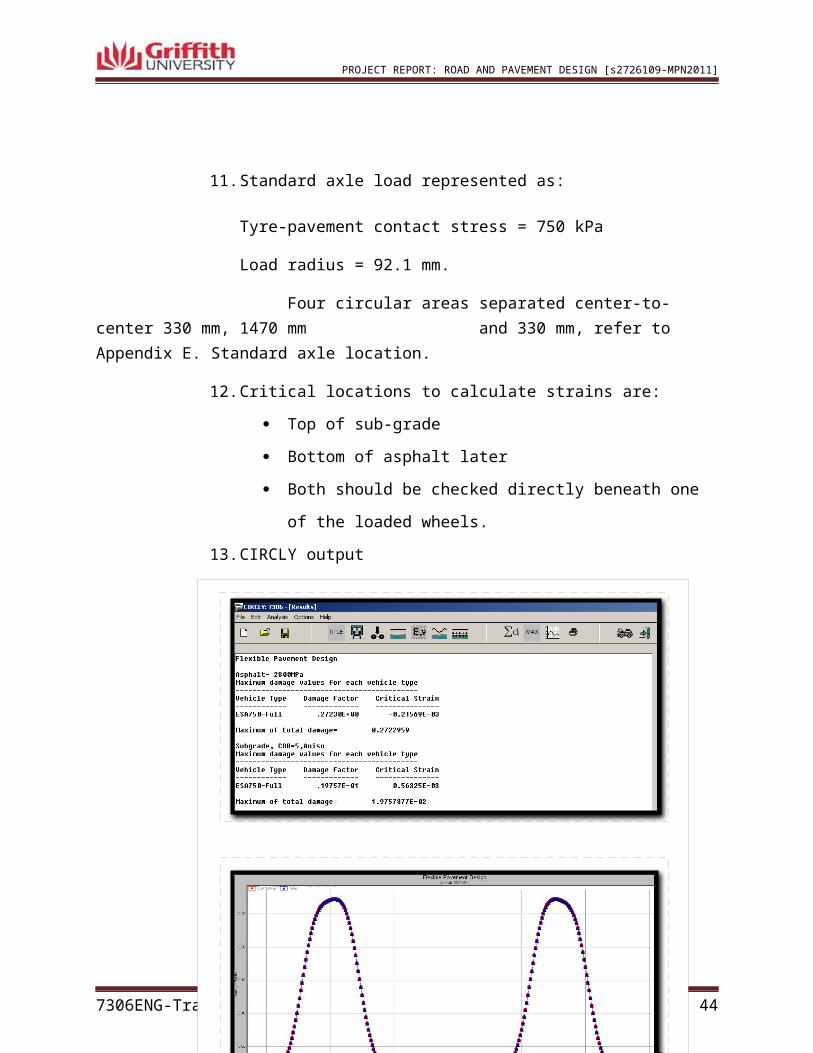
12. Critical locations to calculate strains are:
Top of sub-grade
Bottom of asphalt later
Both should be checked directly beneath one of the loaded wheels.
13. CIRCLY output
7306ENG-Transportation Infrastructure 33
In SummaryDESA = 4.131 x10⁶
DSAR5 = 4.5441 x10⁶
DSAR7 = 6.6096 x10⁶
DSAR12 = 4.957 x10⁷
Result: N=4.96 x10⁶
με = 215.69 from CIRCLY (Figure 3.3 )N=RF∗[6918 (0. 856×Vb+1 .08 )
E0 .36×uε ]5
PROJECT REPORT: ROAD AND PAVEMENT DESIGN [s2726109-MPN2011]
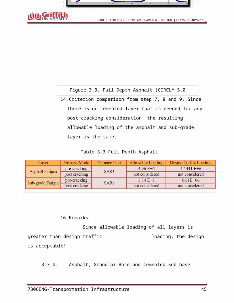
14. Criterion comparison from step 7, 8 and 9. Since there is no cemented layer
that is needed for any post cracking consideration, the resulting allowable
loading of the asphalt and sub-grade layer is the same.
15. Checking of allowable loading versus the design traffic loading.
16. Remarks.
Since allowable loading of all layers is greater than design traffic
loading, the design is acceptable!
7306ENG-Transportation Infrastructure 34
Figure 3.3. Full Depth Asphalt (CIRCLY 5.0 result)
Table 3.3 Full Depth Asphalt
CBR 5 Subgrade
PROJECT REPORT: ROAD AND PAVEMENT DESIGN [s2726109-MPN2011]
3.3.4. Asphalt, Granular Base and Cemented Sub-base
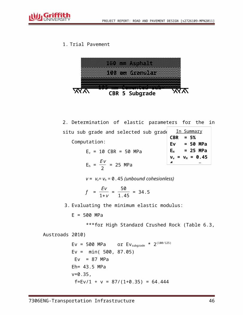
1. Trial Pavement
2. Determination of elastic parameters for the in situ sub grade and selected
sub grade materials:
Computation:
Ev = 10 CBR = 50 MPa
Eh = E v2
= 25 MPa
v = vv= vh = 0.45 (unbound cohesionless)
f = Ev
1+v =
501.45
= 34.5
3. Evaluating the minimum elastic modulus:
E = 500 MPa
***for High Standard Crushed Rock (Table 6.3, Austroads 2010)
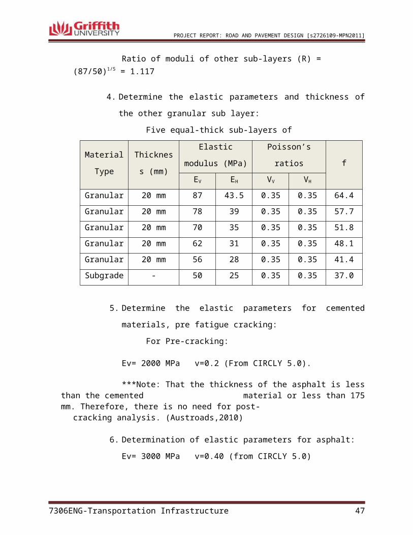
Ev = 500 MPa or Evsubgrade * 2(100/125) Ev = min( 500, 87.05) Ev = 87 MPaEh= 43.5 MPa v=0.35, f=Ev/1 + v = 87/(1+0.35) = 64.444Ratio of moduli of other sub-layers (R) = (87/50)1/5 = 1.117
4. Determine the elastic parameters and thickness of the other granular sub
layer:
7306ENG-Transportation Infrastructure 35
In SummaryCBR = 5%Ev = 50 MPaEH = 25 MPaνv = νH = 0.45f = 34.5
195 mm Cemented sub-base
100 mm Granular base
160 mm Asphalt
PROJECT REPORT: ROAD AND PAVEMENT DESIGN [s2726109-MPN2011]
Five equal-thick sub-layers of
Material
Type
Thickness
(mm)
Elastic modulus
(MPa)Poisson’s ratios
f
EV EH VV VH
Granular 20 mm 87 43.5 0.35 0.35 64.4
Granular 20 mm 78 39 0.35 0.35 57.7
Granular 20 mm 70 35 0.35 0.35 51.8
Granular 20 mm 62 31 0.35 0.35 48.1
Granular 20 mm 56 28 0.35 0.35 41.4
Subgrade - 50 25 0.35 0.35 37.0
5. Determine the elastic parameters for cemented materials, pre fatigue
cracking:
For Pre-cracking:
Ev= 2000 MPa v=0.2 (From CIRCLY 5.0).
***Note: That the thickness of the asphalt is less than the cemented material or less than 175 mm. Therefore, there is no need for post-
cracking analysis. (Austroads,2010)
6. Determination of elastic parameters for asphalt:
Ev= 3000 MPa v=0.40 (from CIRCLY 5.0)
f = Ev
1+v =
30001.40
= 2,142.86
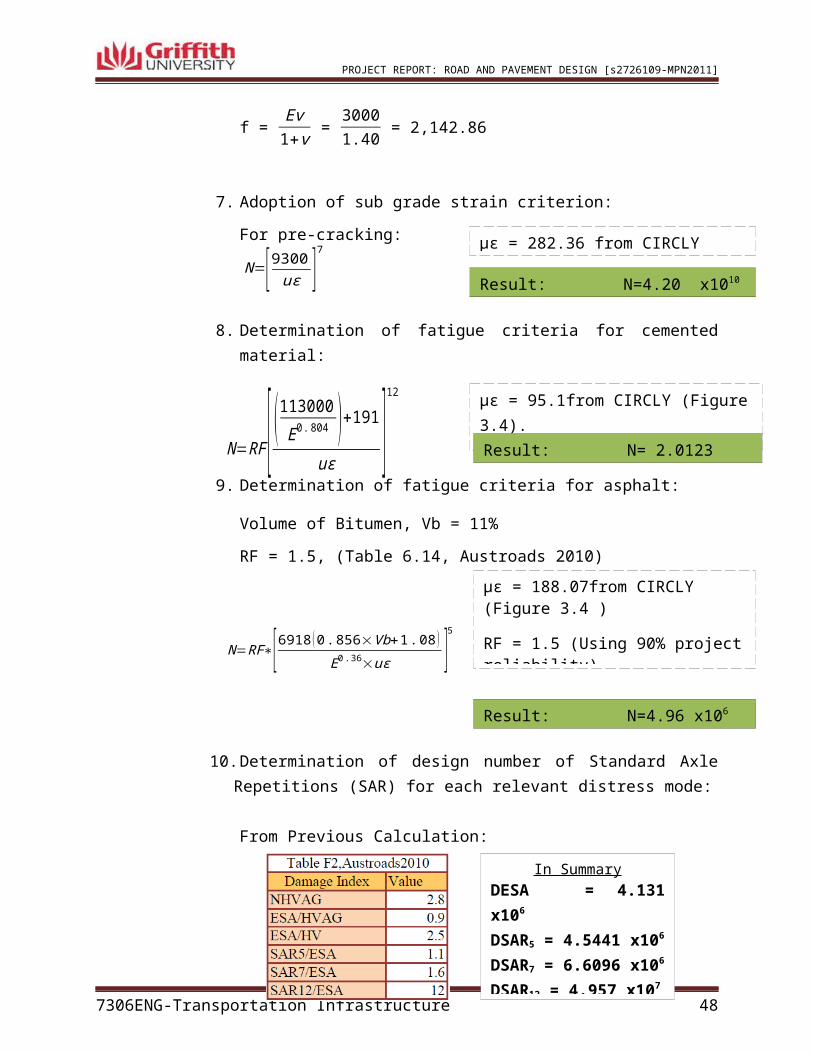
7. Adoption of sub grade strain criterion:
For pre-cracking:
8. Determination of fatigue criteria for cemented material:
7306ENG-Transportation Infrastructure 36
με = 282.36 from CIRCLY (Figure 3.4 )
Result: N=4.20 x10¹⁰
με = 95.1from CIRCLY (Figure 3.4).RF = 2.0 (Using 90% project reliability)E = 2000 MPaResult: N= 2.0123 x10³
N=[9300uε ]
7
N=RF [ (113000E0. 804 )+191
uε ]12
PROJECT REPORT: ROAD AND PAVEMENT DESIGN [s2726109-MPN2011]
9. Determination of fatigue criteria for asphalt:
Volume of Bitumen, Vb = 11%
RF = 1.5, (Table 6.14, Austroads 2010)
10. Determination of design number of Standard Axle Repetitions (SAR) for each relevant distress mode:
From Previous Calculation:
11. Standard axle load represented as:
Tyre-pavement contact stress = 750 kPa
Load radius = 92.1 mm.
Four circular areas separated center-to-center 330 mm, 1470 mm and 330 mm, refer to Appendix E. Standard axle location.
12. Critical locations to calculate strains are:
Top of sub-grade
Bottom of asphalt later
Both should be checked directly beneath one of the loaded wheels.
13. CIRCLY output
7306ENG-Transportation Infrastructure 37
με = 188.07from CIRCLY (Figure 3.4 )
RF = 1.5 (Using 90% project reliability)
E = 3000 MPa
Result: N=4.96 x10⁶
In SummaryDESA = 4.131 x10⁶
DSAR5 = 4.5441 x10⁶
DSAR7 = 6.6096 x10⁶
DSAR12 = 4.957 x10⁷
N=RF∗[6918 (0. 856×Vb+1 .08 )E0 .36×uε ]
5
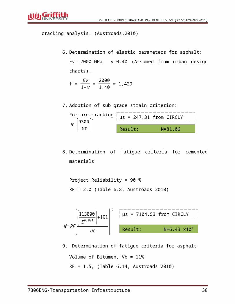
Table 3.4 Asphalt, Granular Base and Cemented Sub-base
PROJECT REPORT: ROAD AND PAVEMENT DESIGN [s2726109-MPN2011]
14. Criterion comparison from step 7, 8 and 9. Since there is no cemented layer
that is needed for any post cracking consideration, the resulting allowable
loading of the asphalt and sub-grade layer is the same.
15. Checking of allowable loading versus the design traffic loading.
16. Remarks.
Since allowable loading of all layers is greater than design traffic
loading, the design is acceptable!
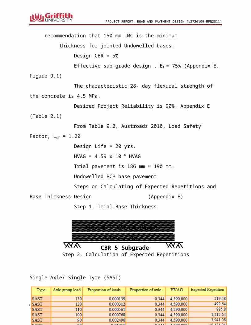
3.4. Rigid Pavement Design
3.4.1. Design Input Parameters
Type of pavement: Plain concrete pavement (PCP)
A concrete shoulder is provided
From Figure 9.1, Austroads 2010, 150 mm lean- mix concrete (LMC)
7306ENG-Transportation Infrastructure 38
Figure 3.4. Asphalt, Granular Base and Cemented Sub-base (CIRCLY 5.0 Resul)
CBR 5 Subgrade
PROJECT REPORT: ROAD AND PAVEMENT DESIGN [s2726109-MPN2011]
***The figure (Appendix E), shows that it is 125mm LMC, but
there is also a recommendation that 150 mm LMC is the
minimum thickness for jointed Undowelled bases.
Design CBR = 5%
Effective sub-grade design , Ef = 75% (Appendix E, Figure 9.1)
The characteristic 28- day flexural strength of the concrete is 4.5 MPa.
Desired Project Reliability is 90%, Appendix E (Table 2.1)
From Table 9.2, Austroads 2010, Load Safety Factor, Lsf = 1.20
Design Life = 20 yrs.
HVAG = 4.59 x 10 6 HVAG
Trial pavement is 186 mm ≈ 190 mm.
Undowelled PCP base pavement
Steps on Calculating of Expected Repetitions and Base Thickness Design
(Appendix E)
Step 1. Trial Base Thickness
Step 2. Calculation of Expected Repetitions
Single Axle/ Single Tyre (SAST)
7306ENG-Transportation Infrastructure 39
186 mm ≈ 190 mm Plain Concrete Pavement150 mm LMC
PROJECT REPORT: ROAD AND PAVEMENT DESIGN [s2726109-MPN2011]
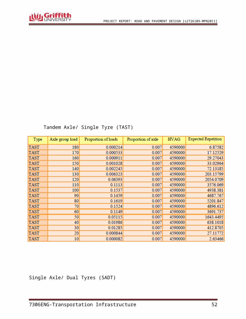
Tandem Axle/ Single Tyre (TAST)
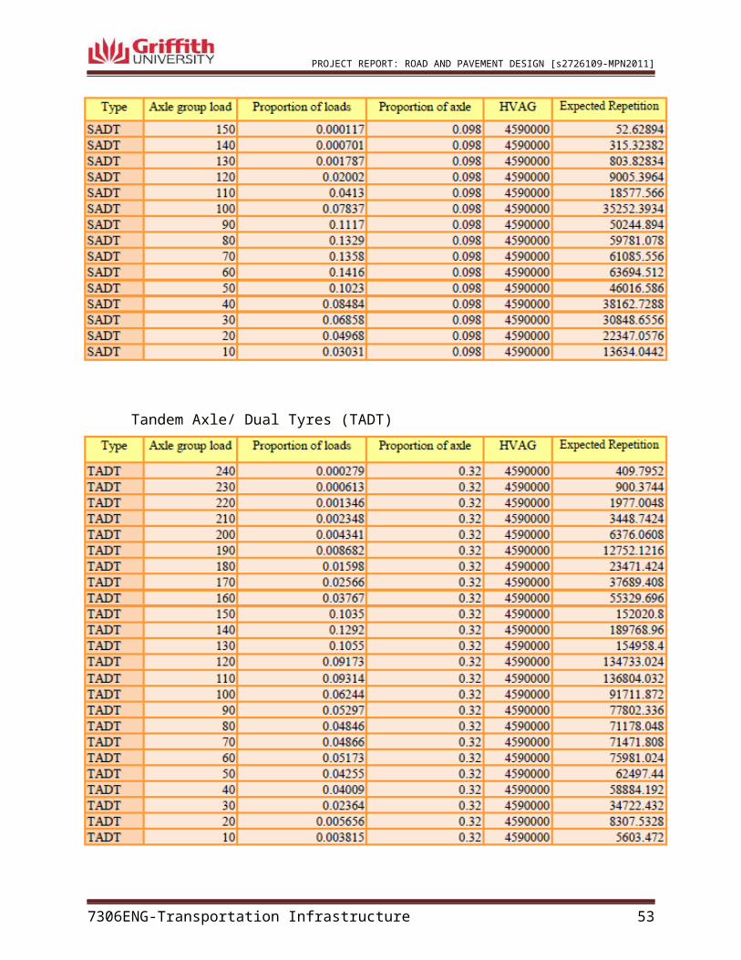
Single Axle/ Dual Tyres (SADT)
7306ENG-Transportation Infrastructure 40
PROJECT REPORT: ROAD AND PAVEMENT DESIGN [s2726109-MPN2011]
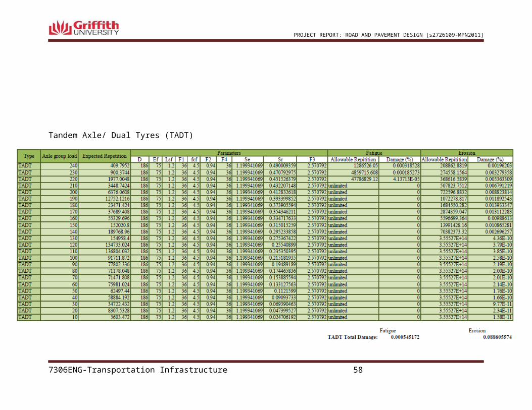
Tandem Axle/ Dual Tyres (TADT)
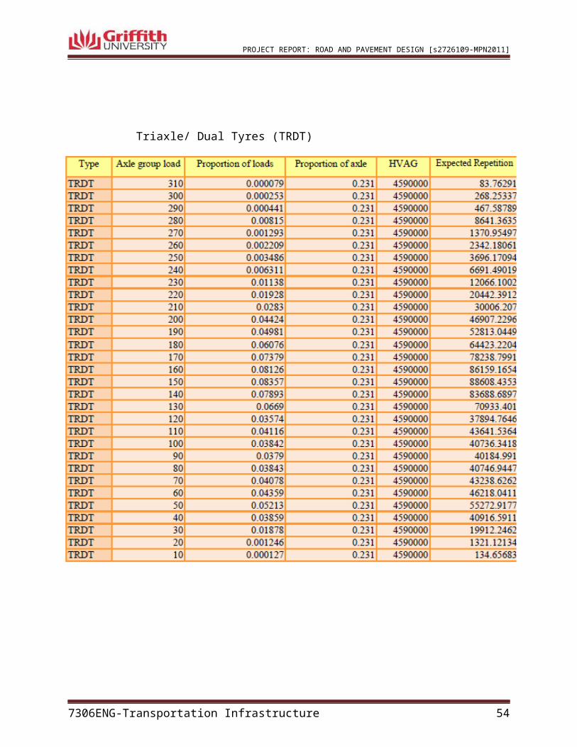
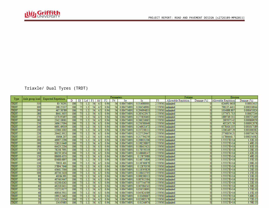
Triaxle/ Dual Tyres (TRDT)
7306ENG-Transportation Infrastructure 41
PROJECT REPORT: ROAD AND PAVEMENT DESIGN [s2726109-MPN2011]
7306ENG-Transportation Infrastructure 42
PROJECT REPORT: ROAD AND PAVEMENT DESIGN [s2726109-MPN2011]
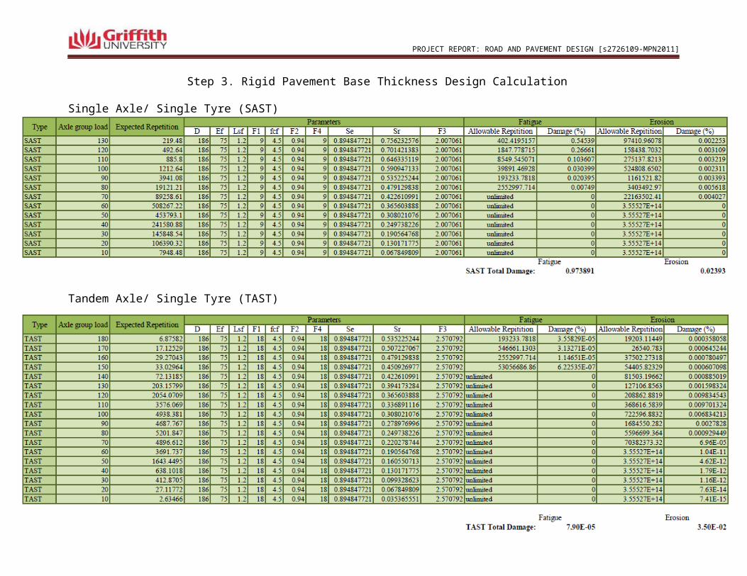
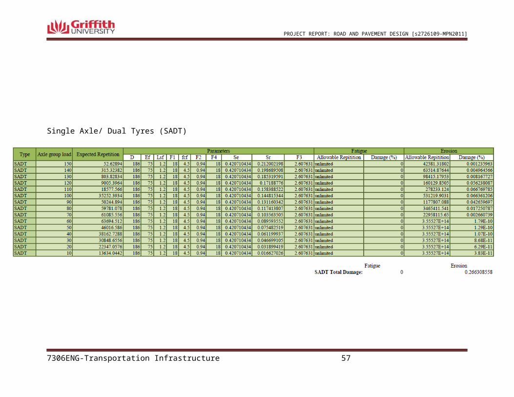
Step 3. Rigid Pavement Base Thickness Design Calculation
Single Axle/ Single Tyre (SAST)
Tandem Axle/ Single Tyre (TAST)
7306ENG-Transportation Infrastructure 43
PROJECT REPORT: ROAD AND PAVEMENT DESIGN [s2726109-MPN2011]
Single Axle/ Dual Tyres (SADT)
7306ENG-Transportation Infrastructure 44
PROJECT REPORT: ROAD AND PAVEMENT DESIGN [s2726109-MPN2011]
Tandem Axle/ Dual Tyres (TADT)
7306ENG-Transportation Infrastructure 45
PROJECT REPORT: ROAD AND PAVEMENT DESIGN [s2726109-MPN2011]
Triaxle/ Dual Tyres (TRDT)
Since, fatigue and erosion percentage of damage is less than 100%, the design is acceptable!
7306ENG-Transportation Infrastructure 46
PROJECT REPORT: ROAD AND PAVEMENT DESIGN [s2726109-MPN2011]
CHAPTER 4: CONCLUSIONS AND RECCOMENDATIONS
A low volume rural road infrastructure needs serious design procedures in terms of its
geometric design and infrastructure sustainability. Main reason is, it is the main access of all
households and will introduce a definite development and improvement to the rural area.
A good road is not just compensating structural analysis but also, it should consider
safety, quality and performance. Generally, the geometric design of this report is normally within
the range of standard specifications. When in terms of sustainability, materials used in the
analysis have been proven for decades to be effective and reliable in terms of different distresses.
The final road design with length of 2.738 kilometers, 3.20 m width two lane- two way
road with a provided concrete shoulder is typically the most suitable design road in the selected
area. It is quite a long road but is intentionally design to introduce a safer environment. Since the
road is almost following to its smooth contour lines of the topography of the area, in terms of
vertical curves, drivers will not experience a very steep road. In terms of cost efficiency, the
chosen geometry provides a minimal gap of length of haulage, and minimal depth of cut and fill
in every road section. As presented in the Mass- Haul Diagram, the negative value of the excess
material represents a cutting activity. In this case, there is no need for the contractor to look for
another filling material. By which, obviously the scenario is advantageous in terms of costing.
Different alternatives were presented in the report but the choice of what would be the
final type of pavement is not decided, considering the fact that, all of the pavement type is
effective and can accommodate the required design traffic load. In actual practice, designers
should advice and recommend the final type of pavement.
. Moreover, it is very important to take note that, no matter how accurate the geometric
and pavement material analysis of the road, the realization of a zero accident road is way too
impossible to achieve. It is practically due to some factors caused by human, facilities or devices,
and other natural occurrences. In other words, the design of roads is just a tool to provide a safer
environment, but safety could be realized basically by its individual cautiousness.
7306ENG-Transportation Infrastructure 47
PROJECT REPORT: ROAD AND PAVEMENT DESIGN [s2726109-MPN2011]
REFERENCES
Austroads (2009). Guide to Road Design- Part 3: Geometric Design, Austroads Incorporated, Sydney, Australia.
Austroads (2010). Guide to Road Design- Part 3: Geometric Design, Austroads Incorporated, Sydney, Australia.
Main Roads ( 2002). Road Planning and Design Manual, Chapter 12- Vertical Alignment
Nepal, K.P (2011). 7306ENG- Transportation Infrastructure Lecture Notes- Griffith University- School of Engineering, Gold Coast, Australia
7306ENG-Transportation Infrastructure 48
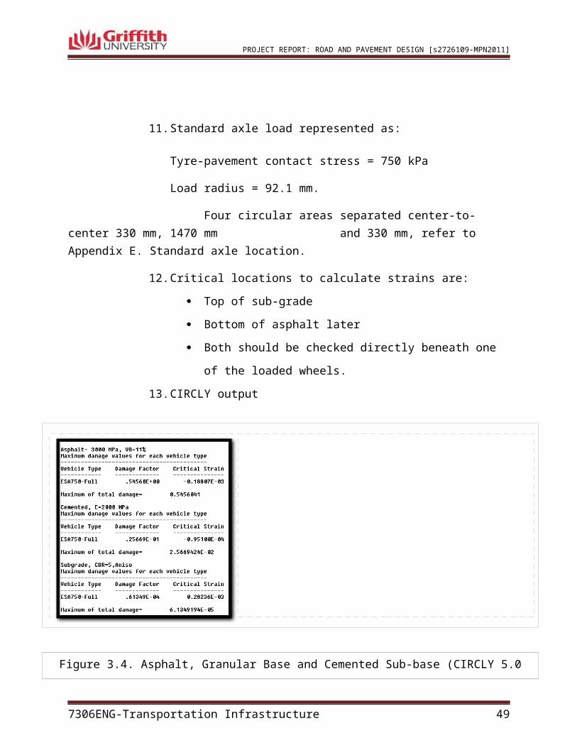
Table A.1. Horizontal Alignment Design Table
PROJECT REPORT: ROAD AND PAVEMENT DESIGN [s2726109-MPN2011]
APPENDIX A
7306ENG-Transportation Infrastructure 49
PROJECT REPORT: ROAD AND PAVEMENT DESIGN [s2726109-MPN2011]
APPENDIX B
7306ENG-Transportation Infrastructure 50
Table B.1. Vertical Alignment Design Table
PROJECT REPORT: ROAD AND PAVEMENT DESIGN [s2726109-MPN2011]
APPENDIX C
7306ENG-Transportation Infrastructure 51
PROJECT REPORT: ROAD AND PAVEMENT DESIGN [s2726109-MPN2011]
7306ENG-Transportation Infrastructure 52
PROJECT REPORT: ROAD AND PAVEMENT DESIGN [s2726109-MPN2011]
7306ENG-Transportation Infrastructure 53
PROJECT REPORT: ROAD AND PAVEMENT DESIGN [s2726109-MPN2011]
7306ENG-Transportation Infrastructure 54
PROJECT REPORT: ROAD AND PAVEMENT DESIGN [s2726109-MPN2011]
7306ENG-Transportation Infrastructure 55
PROJECT REPORT: ROAD AND PAVEMENT DESIGN [s2726109-MPN2011]
APPENDIX D
7306ENG-Transportation Infrastructure 56
PROJECT REPORT: ROAD AND PAVEMENT DESIGN [s2726109-MPN2011]
7306ENG-Transportation Infrastructure 57
PROJECT REPORT: ROAD AND PAVEMENT DESIGN [s2726109-MPN2011]
7306ENG-Transportation Infrastructure 58
PROJECT REPORT: ROAD AND PAVEMENT DESIGN [s2726109-MPN2011]
7306ENG-Transportation Infrastructure 59

PROJECT REPORT: ROAD AND PAVEMENT DESIGN [s2726109-MPN2011]
7306ENG-Transportation Infrastructure 60
PROJECT REPORT: ROAD AND PAVEMENT DESIGN [s2726109-MPN2011]
7306ENG-Transportation Infrastructure 61
PROJECT REPORT: ROAD AND PAVEMENT DESIGN [s2726109-MPN2011]
7306ENG-Transportation Infrastructure 62
PROJECT REPORT: ROAD AND PAVEMENT DESIGN [s2726109-MPN2011]
APPENDIX E
7306ENG-Transportation Infrastructure 63
Table 7.4: Cumulative Growth Factor (CGF) values for below-capacity traffic flow
Standard axle location.
PROJECT REPORT: ROAD AND PAVEMENT DESIGN [s2726109-MPN2011]
Mechanistic Analysis: Input Requierements, Table 8.1 Austroads (2010)
7306ENG-Transportation Infrastructure 64
PROJECT REPORT: ROAD AND PAVEMENT DESIGN [s2726109-MPN2011]
Rigid Pavement Design Calculation
7306ENG-Transportation Infrastructure 65
PROJECT REPORT: ROAD AND PAVEMENT DESIGN [s2726109-MPN2011]
7306ENG-Transportation Infrastructure 66
PROJECT REPORT: ROAD AND PAVEMENT DESIGN [s2726109-MPN2011]
7306ENG-Transportation Infrastructure 67