RR INTERVAL ESTIMATION FROM AN ECG USING A LINEAR ...
106
RR INTERVAL ESTIMATION FROM AN ECG USING A LINEAR DISCRETE KALMAN FILTER by ARUN N JANAPALA B.Tech. Nagarjuna University, 2002 A thesis submitted in partial fulfillment of the requirements for the degree Master of Science in the Department of Electrical and Computer Engineering in the College of Engineering and Computer Science at the University Of Central Florida Orlando, Florida Spring Term 2005
Transcript of RR INTERVAL ESTIMATION FROM AN ECG USING A LINEAR ...

RR INTERVAL ESTIMATION FROM AN ECG USING A LINEAR DISCRETE
KALMAN FILTER
by
ARUN N JANAPALA B.Tech. Nagarjuna University, 2002
A thesis submitted in partial fulfillment of the requirements for the degree Master of Science
in the Department of Electrical and Computer Engineering in the College of Engineering and Computer Science
at the University Of Central Florida Orlando, Florida
Spring Term 2005

ABSTRACT
An electrocardiogram (ECG) is used to monitor the activity of the heart. The human heart
beats seventy times on an average per minute. The rate at which a human heart beats can
exhibit a periodic variation. This is known as heart rate variability (HRV). Heart rate variability is
an important measurement that can predict the survival after a heart attack. Studies have
shown that reduced HRV predicts sudden death in patients with Myocardial Infarction (MI). The
time interval between each beat is called an RR interval, where the heart rate is given by the
reciprocal of the RR interval expressed in beats per minute. For a deeper insight into the
dynamics underlying the beat to beat RR variations and for understanding the overall variance
in HRV, an accurate method of estimating the RR interval must be obtained. Before an HRV
computation can be obtained the quality of the RR interval data obtained must be good and
reliable. Most QRS detection algorithms can easily miss a QRS pulse producing unreliable RR
interval values. Therefore it is necessary to estimate the RR interval in the presence of missing
QRS beats. The approach in this thesis is to apply KALMAN estimation algorithm to the RR
interval data calculated from the ECG. The goal is to improve the RR interval values obtained
from missed beats of ECG data.
ii

ACKNOWLEDGEMENTS
I am honored to have had the opportunity to work with Dr. Weeks as my thesis advisor. I
thank him for the best gift of all, that of learning.
I would like to thank Dr. Bauer and Dr. Klee for their time and support in serving as my thesis
committee members.
I would like to thank my parents who have sacrificed so much to give me a good education. I
thank them for all they have done for me.
I would also like to thank my friends Pavan, Akarsh , Rahul and Sash for their constant
support and help throughout the period of my research.
Finally I would like to thank Deepthi. Without her constant love and support throughout my
time here, this thesis would not have been possible.
iii

TABLE OF CONTENTS
LIST OF FIGURES ................................................................................................................................. vi LIST OF TABLES.................................................................................................................................. viii CHAPTER 1: INTRODUCTION ........................................................................................................ 1
Objective ............................................................................................................................................... 1 Functioning of heart ........................................................................................................................... 2 ECG background ................................................................................................................................ 5 Heart Rate ............................................................................................................................................. 8 Arrhythmia............................................................................................................................................ 8 Heart rate detection............................................................................................................................. 9
CHAPTER 2: DISCUSSION OF THE KALMAN FILTER ....................................................... 12
Introduction........................................................................................................................................ 12 Mean squared error ........................................................................................................................... 14 MSE solution...................................................................................................................................... 15 Steepest Descent Algorithm............................................................................................................ 18 Least mean square (LMS) algorithm.............................................................................................. 21 KALMAN Filter Derivation ........................................................................................................... 22 Filter Algorithm ................................................................................................................................. 27
CHAPTER 3: KALMAN FILTER IMPLEMENTATION .......................................................... 30 Implementation.................................................................................................................................. 30 Filter Parameters................................................................................................................................ 30 Filter adaptation................................................................................................................................. 31 Performance in noisy environment................................................................................................ 37 Filter performance with different parameters .............................................................................. 39 Statistics ............................................................................................................................................... 46
CHAPTER 4: IMPLEMENTATION ON ECG RECORDINGS.............................................. 48
Implementation setup....................................................................................................................... 48 A Real Time QRS Detection Algorithm....................................................................................... 48 Results for real ECG data ................................................................................................................ 51
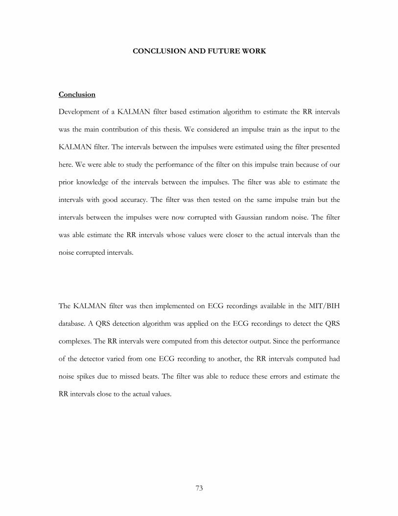
CONCLUSION AND FUTURE WORK......................................................................................... 73
Conclusion .......................................................................................................................................... 73 Future Work ....................................................................................................................................... 74
iv

APPENDIX A: SIMULATED DATA............................................................................................... 75 APPENDIX B: MATLAB SOURCE CODE................................................................................... 83 LIST OF REFERENCES...................................................................................................................... 97
v

LIST OF FIGURES
Figure 1.1: HRV analysis ........................................................................................................................... 1
Figure 1.2: HRV analysis with estimated RR intervals ........................................................................ 2
Figure 1.3: Anatomy of Human Heart .................................................................................................. 3
Figure 1.4: Cardiac conduction system .................................................................................................. 4
Figure 1.5: Pacemaker cell action potential............................................................................................ 6
Figure 1.6: Non Pacemaker cell action potential .................................................................................. 6
Figure 1.7: Action potentials at different parts of the heart .............................................................. 7
Figure 1.8: ECG wave .............................................................................................................................. 7
Figure 2.1: Mean Square Error............................................................................................................... 15
Figure 2.2: Non Recursive Adaptive Filter .......................................................................................... 17
Figure 2.3: KALMAN Estimator .......................................................................................................... 28
Figure 3.2: Test Signal ................................................................................................................................ 33
Figure 3.3: Intervals of the test signal ................................................................................................... 34
Figure 3.4: Estimated Interval ................................................................................................................ 34
Figure 3.5: Comparison of the estimated interval with actual interval ........................................... 35
Figure 3.6: Estimation Error .................................................................................................................. 36
Figure 3.7: KALMAN Gain ................................................................................................................... 37
Figure 3.8: Performance of the filter with a noisy input ................................................................... 38
Figure 3.9: Effect of the filter estimation with variation of the Measurement noise .................. 40
Figure 3.10: Variation in estimation Error with variation in measurement Noise Covariance 41
Figure 3.11: Defining the filter delay..................................................................................................... 42
Figure 3.12: Variation of the filter delay with variation in Measurement Noise Covariance ..... 42
vi
Figure 3.13: Filter performance with the process noise covariance assumed to be 10 ............... 43
Figure 3.14: Variation in mean estimation error with variation in Process Noise Covariance .. 44
Figure 3.15: Variation of the filter delay with variation in the Process Noise Covariance ......... 45
Figure 4.1: Estimation of RR intervals from ECG recordings ........................................................ 48
Figure 4.3: ECG and the QRS detector plot for file 100.dat ........................................................... 53
Figure 4.4: Measured Intervals and Estimated intervals for file 100.dat........................................ 54
Figure 4.5: ECG and the QRS detector plot for the file 101.dat..................................................... 55
Figure 4.6: Measured Intervals and Estimated intervals for file 101.dat........................................ 56
Figure 4.7: ECG and QRS detector plots for file 102.dat................................................................. 57
Figure 4.8: Measured Intervals and Estimated intervals for file 102.dat........................................ 58
Figure 4.9: ECG and QRS detector plot for file 103.dat .................................................................. 59
Figure 4.10: Measured Intervals and Estimated intervals for file 103.dat...................................... 60
Figure 4.11: ECG and QRS detector plot for file 104.dat ................................................................ 61
Figure 4.12: Measured Intervals and Estimated intervals for file 104.dat...................................... 62
Figure 4.13: ECG and QRS detector plot for file 105.dat ................................................................ 63
Figure 4.14: Measured Intervals and Estimated intervals for file 105.dat...................................... 64
Figure 4.15: ECG and QRS detector for file 106.dat ........................................................................ 65
Figure 4.16: Measured Intervals and Estimated intervals for file 106.dat...................................... 66
Figure 4.17: ECG and QRS detector for file 107.dat ........................................................................ 67
Figure 4.18: Measured Intervals and Estimated intervals for file 107.dat...................................... 68
Figure 4.19: ECG and QRS detector plot for file 118.dat ................................................................ 69
Figure 4.20: Measured Intervals and Estimated intervals for file 118.dat...................................... 70
Figure 4.21: ECG and QRS detector plot for file 119.dat ................................................................ 71
Figure 4.22: Measured Intervals and Estimated intervals for file 119.dat...................................... 72
vii
LIST OF TABLES
Table 3.1: Statistics of measured and estimated RR intervals .......................................................... 46 Table 4.1: Filter parameters for the ECG recordings ........................................................................ 52 Table A1: Comparison of Estimated intervals with Measured Intervals for beat 1 to 36 .......... 76 Table A2: Comparison of Estimated intervals with Measured Intervals for beat 37 to 73........ 77 Table A3: Comparison of Estimated intervals with Measured Intervals for beat 74 to 107...... 78 Table A4: Comparison of Estimated intervals with Measured Intervals for beat 108 to 140 ... 79 Table A5: Comparison of Estimated intervals with Measured Intervals for beat 141 to 171 ... 80 Table A6: Comparison of Estimated intervals with Measured Intervals for beat 172 to 204 ... 81 Table A7: Comparison of Estimated intervals with Measured Intervals for beat 205 to 230 ... 82
viii

CHAPTER 1: INTRODUCTION
Objective
The rate at which the human heart beats exhibits a periodic variation. This is known as heart
rate variability (HRV). Heart rate variability is an important measurement that can predict the
survival after a heart attack. Studies have shown that reduced HRV predicts sudden death in
patients with Myocardial Infarction (MI).
The HRV is originally measured from the R-R interval data calculated from the ECG. Figure
1.1 gives the steps in calculating HRV. First an ECG recording of a patient is obtained. Next,
the QRS part of the ECG is detected and the RR interval is calculated. From the RR interval
the HRV is found.
ECG
recording R-R interval
Figure 1.1: HRV analysis
However before the R-R interval undergoes the HRV computation we have to make sure that
the quality of the R-R interval data is good and reliable. There might be a possibility for a QRS
Patient Calculation HRV
analysis
1

detection algorithm to miss a beat. This type of error usually results in unreliable HRV
measurement. Therefore it is necessary to first filter the R-R interval sequence based on some
algorithm and then submit the newly obtained data for HRV analysis.
The KALMAN estimation algorithm has been used on the R-R interval data, which estimates
the R-R intervals with minimum prediction error based on the previous values of the R-R
interval. This algorithm was tested on different ECG recordings and its performance has been
studied in this thesis. Figure 1.2 shows the addition of the RR interval estimation in the HRV
process hence improving the HRV analysis.
Figure 1.2: HRV analysis with estimated RR intervals
Functioning of heart
The Cardiovascular system is responsible for the supply of blood which is full of oxygen and
nutrients to each and every part of the human body. The most crucial organ in this system is
the human heart. It is the heart that pumps blood through the entire body by contracting and
relaxing its muscular walls continuously. The human heart is made up of four chambers: Right
Atrium (RA), Left Atrium (LA), Right Ventricle (RV), Left Ventricle (LV). The impure blood
Patient
ECG
recording
R-R interval
Calculation
R-R interval
estimation
HRV
analysis
2
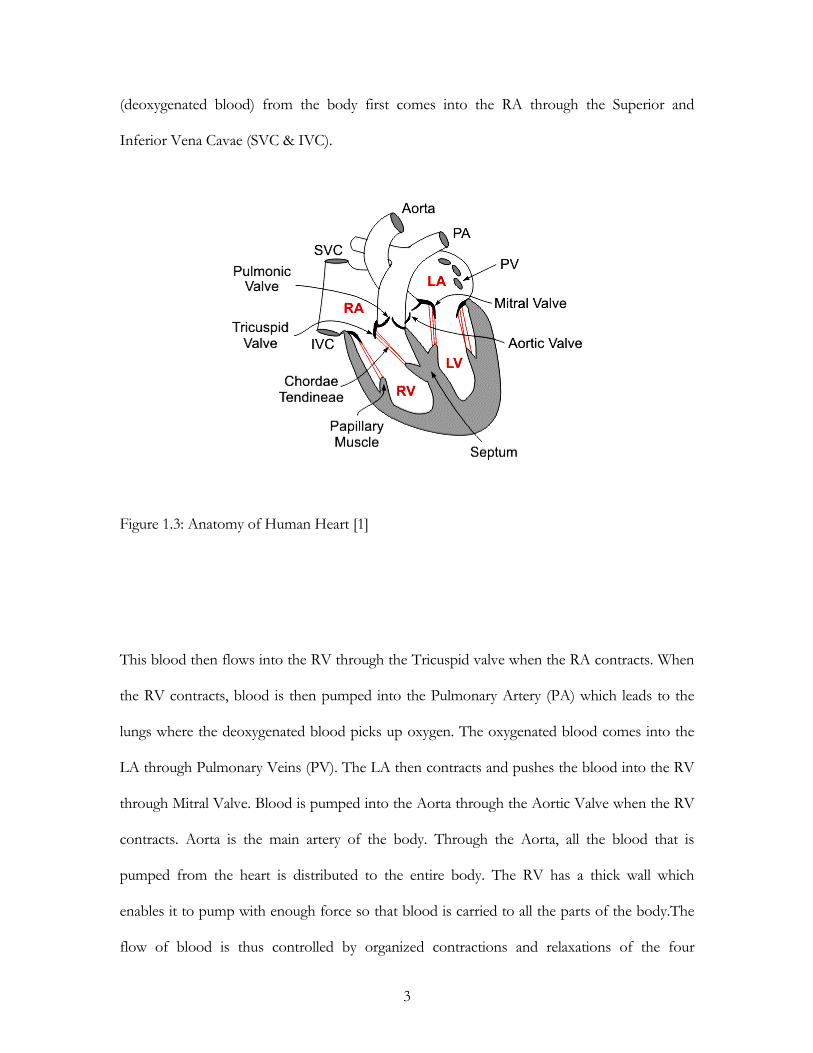
(deoxygenated blood) from the body first comes into the RA through the Superior and
Inferior Vena Cavae (SVC & IVC).
Figure 1.3: Anatomy of Human Heart [1]
This blood then flows into the RV through the Tricuspid valve when the RA contracts. When
the RV contracts, blood is then pumped into the Pulmonary Artery (PA) which leads to the
lungs where the deoxygenated blood picks up oxygen. The oxygenated blood comes into the
LA through Pulmonary Veins (PV). The LA then contracts and pushes the blood into the RV
through Mitral Valve. Blood is pumped into the Aorta through the Aortic Valve when the RV
contracts. Aorta is the main artery of the body. Through the Aorta, all the blood that is
pumped from the heart is distributed to the entire body. The RV has a thick wall which
enables it to pump with enough force so that blood is carried to all the parts of the body.The
flow of blood is thus controlled by organized contractions and relaxations of the four
3

chambers of the heart. The Electrical impulses generated by the heart tissue allow these heart
chambers to contract and relax in a continuous fashion. The heart has its own electrical system
called as cardiac conduction system.
Image copyright 2000 Texas Heart Institute, www.texasheartinstitute.org
Figure 1.4: Cardiac conduction system [2]
The Sinoatrial Node (SA) which is also called as the natural pacemaker initiates the heart beat by
sending out an electrical impulse. The movement of these electrical signals makes the muscles
contract. Once the signal diminishes, the heart muscles relax. The signal generated by the SA
Node first passes through the muscles of LA and RA, thus making it contract. The electrical
signal then proceeds to the Atrioventricular Node (AV) and pauses there for while - giving the
Ventricles sometime to fill with blood. The electrical signal is then relayed down to the
Ventricles through a conducting tissue called Bundle of His, which branches into two pathways -
4
left and right bundle branches that supply to the Ventricles - making it to contract and pump
the blood.
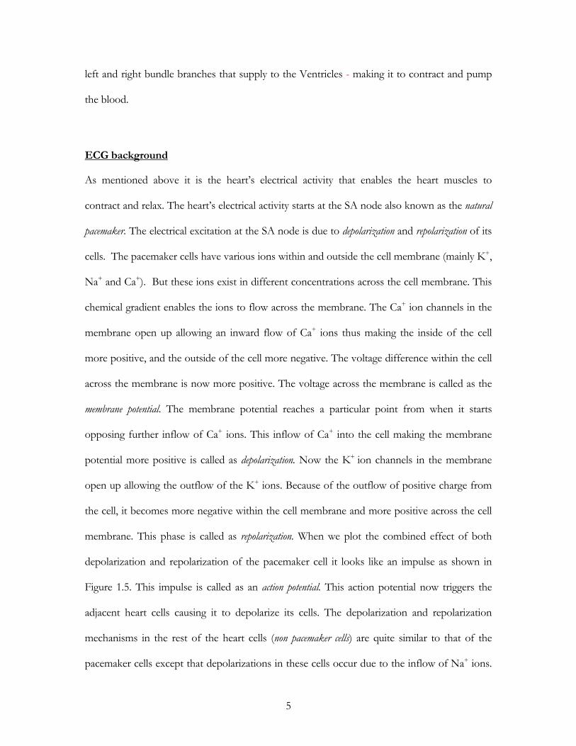
ECG background
As mentioned above it is the heart’s electrical activity that enables the heart muscles to
contract and relax. The heart’s electrical activity starts at the SA node also known as the natural
pacemaker. The electrical excitation at the SA node is due to depolarization and repolarization of its
cells. The pacemaker cells have various ions within and outside the cell membrane (mainly K+,
Na+ and Ca+). But these ions exist in different concentrations across the cell membrane. This
chemical gradient enables the ions to flow across the membrane. The Ca+ ion channels in the
membrane open up allowing an inward flow of Ca+ ions thus making the inside of the cell
more positive, and the outside of the cell more negative. The voltage difference within the cell
across the membrane is now more positive. The voltage across the membrane is called as the
membrane potential. The membrane potential reaches a particular point from when it starts
opposing further inflow of Ca+ ions. This inflow of Ca+ into the cell making the membrane
potential more positive is called as depolarization. Now the K+ ion channels in the membrane
open up allowing the outflow of the K+ ions. Because of the outflow of positive charge from
the cell, it becomes more negative within the cell membrane and more positive across the cell
membrane. This phase is called as repolarization. When we plot the combined effect of both
depolarization and repolarization of the pacemaker cell it looks like an impulse as shown in
Figure 1.5. This impulse is called as an action potential. This action potential now triggers the
adjacent heart cells causing it to depolarize its cells. The depolarization and repolarization
mechanisms in the rest of the heart cells (non pacemaker cells) are quite similar to that of the
pacemaker cells except that depolarizations in these cells occur due to the inflow of Na+ ions.
5
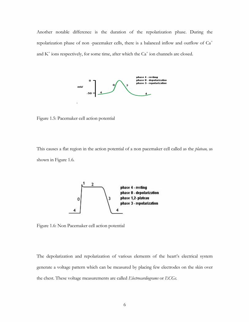
Another notable difference is the duration of the repolarization phase. During the
repolarization phase of non -pacemaker cells, there is a balanced inflow and outflow of Ca+
and K+ ions respectively, for some time, after which the Ca+ ion channels are closed.
Figure 1.5: Pacemaker cell action potential
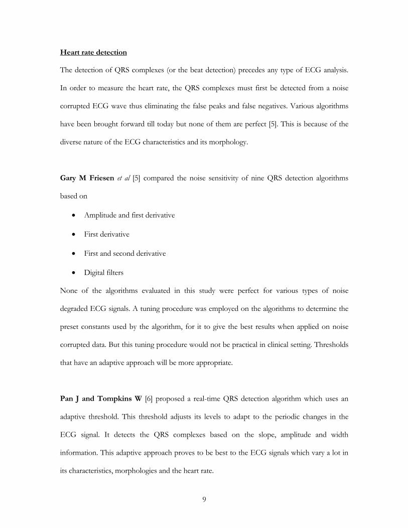
This causes a flat region in the action potential of a non pacemaker cell called as the plateau, as
shown in Figure 1.6.
Figure 1.6: Non Pacemaker cell action potential
The depolarization and repolarization of various elements of the heart’s electrical system
generate a voltage pattern which can be measured by placing few electrodes on the skin over
the chest. These voltage measurements are called Electrocardiograms or ECGs.
6

The ECG wave has various segments as shown in Figure 1.8 each representing some particular
action of the heart.
P wave: This part of the ECG wave is the result of the atrial contraction.
QRS complex: The QRS complex represents the ventricular activation.
Figure 1.7: Action potentials at different parts of the heart
Figure 1.8: ECG wave [4]
T wave: This portion of the ECG wave represents the ventricular relaxation.
7

The popular ECG systems at present are the 12 lead, 5 lead and 3 lead ECGs [15]. The leads
record the heart’s electric field in different angles.
Heart Rate
It is the number of heart beats per minute. The time interval between each beat is the R wave
to R wave interval, in short called as RR interval. Therefore heart rate is given by the reciprocal
of the RR interval expressed in beats per minute. A normal heart beats 60 to 100 times a
minute.
Arrhythmia
Any deviation from the normal heart rhythm or irregular heart beat due to a malfunction in the
heart’s conduction system is called as arrhythmia. The two major types of arrhythmia are
Bradycardia and Tachycardia.
Bradycardia: If the heart beat is below 60 beats per minute which is considered to be very
slow then the heart is said to be suffering from Bradycardia.
Tachycardia: If the heart beat is above 100 beats per minute which is considered to be very
high then the heart is said to be suffering from Tachycardia.
Both Bradycardia and Tachycardia are medically significant. There are other arrhythmias like
the sinus arrhythmia and sinus tachycardia which are not medically significant.
Sinus arrhythmia: It is the variation in the heart rhythm during breathing.
Sinus tachycardia: It is the speeding up of the heart rate during any physical exercise.
8
Heart rate detection
The detection of QRS complexes (or the beat detection) precedes any type of ECG analysis.
In order to measure the heart rate, the QRS complexes must first be detected from a noise
corrupted ECG wave thus eliminating the false peaks and false negatives. Various algorithms
have been brought forward till today but none of them are perfect [5]. This is because of the
diverse nature of the ECG characteristics and its morphology.
Gary M Friesen et al [5] compared the noise sensitivity of nine QRS detection algorithms
based on
• Amplitude and first derivative
• First derivative
• First and second derivative
• Digital filters
None of the algorithms evaluated in this study were perfect for various types of noise
degraded ECG signals. A tuning procedure was employed on the algorithms to determine the
preset constants used by the algorithm, for it to give the best results when applied on noise
corrupted data. But this tuning procedure would not be practical in clinical setting. Thresholds
that have an adaptive approach will be more appropriate.
Pan J and Tompkins W [6] proposed a real-time QRS detection algorithm which uses an
adaptive threshold. This threshold adjusts its levels to adapt to the periodic changes in the
ECG signal. It detects the QRS complexes based on the slope, amplitude and width
information. This adaptive approach proves to be best to the ECG signals which vary a lot in
its characteristics, morphologies and the heart rate.
9
Ivaylo I Christov [7] has developed a real-time QRS detection using combined adaptive
threshold. The adaptive threshold used in this algorithm combines three parameters.
• An adaptive slew rate
• A parameter which rises when noise with very high frequency occurs
• A parameter to avoid missing heart beats with unusually low amplitudes
This algorithm compares the absolute value of this adaptive threshold and the sum of the
differentiated ECG from different leads, for the QRS detection. Sensitivity (Se) of 99.69% and
Specificity (Sp) of 99.66% has been achieved using this algorithm.
Se and Sp can be defined as
Se = TP / (TP+FN) (1.1)
Sp= TP / (TP+FP) (1.2)
TP is true positive, FN and FP are the false negative and false positive respectively.
Afonso et al [8] have developed a multi rate digital signal processing algorithm to detect heart
beats in the ECG. This algorithm incorporates a filter bank which contains a set of filters.
These filters decompose the incoming ECG signal into various sub bands. Each sub band will
carry some particular information regarding the ECG. These sub bands are then processed
individually based on the specific application. For example major proportion of the QRS
complex energy extends to the 40 Hz frequency. If a QRS complex is originated at the SA
node its energy will be appearing in the higher frequency sub bands. Therefore by analyzing
different sub bands of the ECG, beat can be detected.
10
In this thesis, based on the pulses generated by the QRS detection algorithm by Pan J,
Tompkins W the R-R interval has been estimated using a KALMAN estimator. KALMAN filter
derivation and its applications are discussed in detail in the following chapter. The KALMAN
filter presented in this thesis was implemented in MATLAB.
The filter presented here was first tested on a few test signals and its performance was studied.
The results are included in Chapter 3. The filter was then used on the ECG recordings
available in the MIT/BIH ECG data base [20]. Ten ECG recordings were selected from the
database to test the KALMAN filter. The results are shown in chapter 4.
11
CHAPTER 2: DISCUSSION OF THE KALMAN FILTER
Introduction
The estimation theory started to develop when the need to estimate the motion of the
heavenly bodies from a set of noisy telescopic measurements [9] arose. To solve this problem,
the method of least squares was used which was invented by Karl Friedrich Gauss. One method is
based on KALMAN filtering [10] and is considered a modern form of this least squares
estimation technique.
The purpose of the KALMAN filter is to estimate the accurate information from inaccurate
data. It essentially estimates the state of a system based on the system output measurements
which contain random errors. It is extensively used in the areas of navigational science,
tracking, signal processing and control theory. The major applications where the KALMAN
filter plays a vital role are vehicle navigation, satellite orbit estimation, radar tracking, filtering
and estimation of signals and real time control of machines. In the following few paragraphs
interesting proposals of the application of the KALMAN filter are discussed.
M.P.Taravainen et al [11] in their paper "Estimation of Non Stationary EEG spectrum with
KALMAN Filter" published in 2003, discuss an adaptive spectrum estimation method for
non-stationary EEG. Since the EEG signals are non-stationary, a parametrical spectral analysis
method was used which is based on a time varying auto regressive moving average (ARMA)
model. The KALMAN filter algorithm was used in the estimation of the parameters for the
above time varying model.
12

The KALMAN filter also has interesting applications in the field of Communications. It can
be used in the estimation of the round trip time in communication networks. This application
has been discussed in detail in the paper "Round Trip Time Estimation in Communication
Networks using adaptive KALMAN filtering" by Krister Jacobsson et al [12]. The round trip
time in the communication network plays an important role in the congestion control.
Therefore the more accurate the round trip time estimates are the more efficient is the
congestion control. The round trip time is usually measured from packet acknowledgements,
which include delays caused by the network transient effects. This makes the measured round
trip time less accurate. The KALMAN filter in conjunction with a change detection algorithm
was used to get more accurate estimates of the round trip times and the results showed that
the estimates are more accurate when compared to the round trip time estimator currently
used in TCP [12].
The paper "Real time Estimation of Human Body Postures using KALMAN filter" by
Kazuhiko Taka Hashi et al [13] proposes the usage of KALMAN filter while estimating the
postures of human body, which is very important especially for machine-user interface. While
estimating the human body postures using the silhouette based estimation method problems
such as self occlusion occur. In silhouette based estimation method, the feature points of the
human body (like the top of the head, tips of hands and feet, and elbow, knee joints) are
obtained from the human silhouettes (outline images). The problem of self occlusion occurs in
certain postures like when the hands overlap the body. It is difficult to obtain the feature
points in such cases. An autoregressive model has been used to track and obtain these feature
points. The parameters of the AR model are estimated using the KALMAN filter [13].
13

R.E. KALMAN published his famous paper [10] in 1960, “A new approach to linear filtering and
prediction problems” in which he described a recursive algorithm that solves the discrete data
linear filtering problem. It is an efficient computational solution of the method of least
squares. The filter was constructed with the goal to minimize the mean squared error [10].
Mean squared error
Consider a signal yk and its estimate from the estimator is ŷk. The error in estimation is given
by
ek = yk - ŷk (2.1)
Therefore the error is amount of deviation of the estimated signal from the true signal.
The squared error function is defined as
f (ek) = (yk - ŷk)2 (2.2)
Since we have to consider the ability of the filter over a period of time, a more appropriate
metric would be the expected value of the squared error function. This metric is named as the
loss function.
loss function = E{ f (ek) } (2.3)
This leads us to the mean square error (MSE)
εk = E{ ek2} (2.4)
14
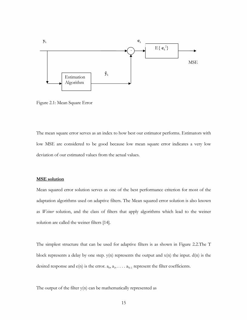
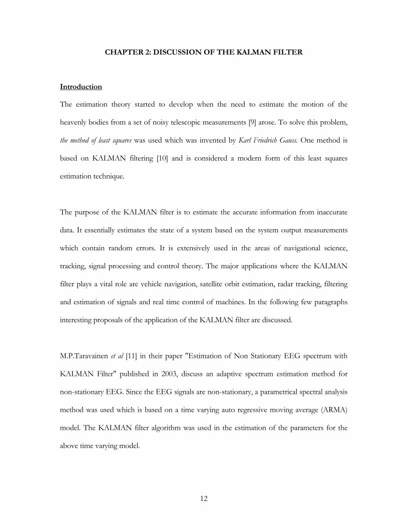
Figure 2.1: Mean Square Error
The mean square error serves as an index to how best our estimator performs. Estimators with
low MSE are considered to be good because low mean square error indicates a very low
deviation of our estimated values from the actual values.
MSE solution
Mean squared error solution serves as one of the best performance criterion for most of the
adaptation algorithms used on adaptive filters. The Mean squared error solution is also known
as Weiner solution, and the class of filters that apply algorithms which lead to the weiner
solution are called the weiner filters [14].
The simplest structure that can be used for adaptive filters is as shown in Figure 2.2.The T
block represents a delay by one step. y(n) represents the output and x(n) the input. d(n) is the
desired response and e(n) is the error. a0, a1, . . . . aN-1 represent the filter coefficients.
The output of the filter y(n) can be mathematically represented as
Estimation Algorithm
¯E{ ek
2}yk ek
MSE
ŷk
15
y(n) = xTnan (2.5)
N
filter coefficient vector at any time instant n.
e(n) = d(n) – y(n) (2.6)
d(n) is the d
ean square error (MSE) is given by
(2.7)
n) = E[ d2(n) – 2d(n)y(n) + y2(n)] (2.8)
for a filter with fixed coeff
nxnT ] an (2.10)
If by
(2.11)
If
(2.12)
Substituting Equations 2. xpressed as
(2.13)
is the length of the filter.
an = [ a0 a1 a2 …. aN-1]T is the
xn = [ x1 x2 x3 ….. xN-1]T is the input vector at any time instant n.
The error function is given by e(n) where
esired response.
Based on Equation 2.4 the m
ε(an) = E{ e(n)2}
substituting Equation 2.6 in 2.7
ε(a
ε(an) = E[ d2(n) ] – 2E[ d(n)anTxn ] + E[ an
TxnxnTan ] (2.9)
icients the MSE function is given by
ε(an) = E[ d2(n) ] – 2anTE[ d(n) xn ] + an
TE[ x
pn is the cross correlation of the desired response and the input then it is given
pn = E[ d(n) xn ]
the correlation of the input x(n) is given by Rn then it is given by
Rn = E[ xnxnT ]
11 and 2.12 in 2.10 the MSE can be e
ε(an) = E[ d2(n) ] - 2anTpn + an
TRn an
16
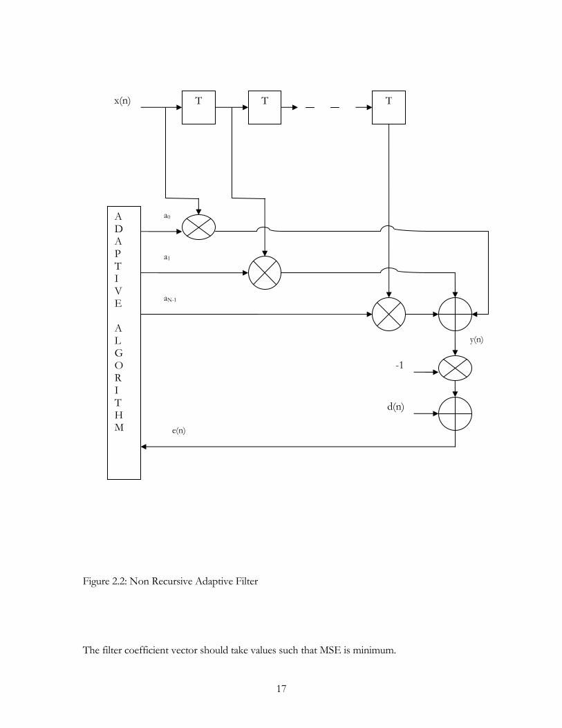
Figure 2.2: Non Recursive Adaptive Filter
The filter coefficient vector should take values such that MSE is minimum.
T T T
A D A P T I V E A L G O R I T H M
x(n)
a0
a1
aN-1
y(n)
-1
d(n)
e(n)
17
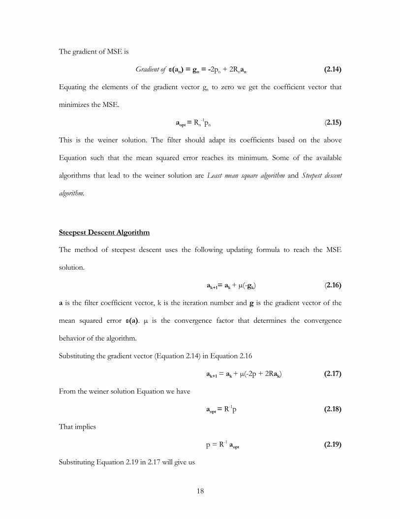
The gradient of MSE is
Gradient of ε(an) = gn = -2pn + 2Rnan (2.14)
Equating the elements of the gradient vector gn to zero we get the coefficient vector that
minimizes the MSE.
aopt = Rn-1pn (2.15)
This is the weiner solution. The filter should adapt its coefficients based on the above
Equation such that the mean squared error reaches its minimum. Some of the available
algorithms that lead to the weiner solution are Least mean square algorithm and Steepest descent
algorithm.
Steepest Descent Algorithm
The method of steepest descent uses the following updating formula to reach the MSE
solution.
ak+1= ak + µ(-gk) (2.16)
a is the filter coefficient vector, k is the iteration number and g is the gradient vector of the
mean squared error ε(a). µ is the convergence factor that determines the convergence
behavior of the algorithm.
Substituting the gradient vector (Equation 2.14) in Equation 2.16
ak+1 = ak + µ(-2p + 2Rak) (2.17)
From the weiner solution Equation we have
aopt = R-1p (2.18)
That implies
p = R-1 aopt (2.19)
Substituting Equation 2.19 in 2.17 will give us
18
ak+1 = ak -2µR(ak - aopt) (2.20)
The error in the filter coefficients when compared to the optimal filter coefficients can be
represented as
vk = ak - aopt (2.21)
Equation 2.20 can now be represented as
vk+1 = (I - 2 µR) vk (2.22)
The above Equation is pre-multiplied by QT where Q is a unitary matrix that diagnolizes R.
QT vk+1 = (I - 2µQTRQ)QTvk (2.23)
The coefficient error vector v is rotated to the principal axis by the following transformation
v’k+1 = QT vk+1 (2.24)
Equation 2.23 now can be rewritten as
v’k+1 = (I - 2µΛ) v’
k (2.25)
Λ is the eigenvalue matrix of the input correlation matrix R. [15] By mathematical induction
the solution to Equation 2.25 must be
v’k = (I - 2µΛ)k v’
0 (2.26)
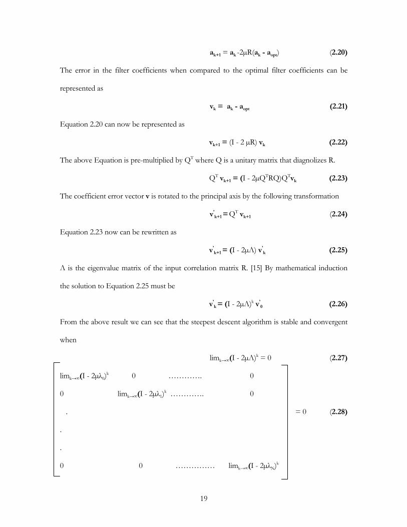
From the above result we can see that the steepest descent algorithm is stable and convergent
when
limk→∞(I - 2µΛ)k = 0 (2.27)
limk→∞(I - 2µλ0)k 0 …………. 0
0 limk→∞(I - 2µλ1)k …………. 0
. = 0 (2.28)
.
.
0 0 …………… limk→∞(I - 2µλN)k
19
where λ0, λ1, …. λN are the eigen values of R.
From the above form we see that the convergence condition is satisfied by choosing µ so that
0 < µ < 1/λmax (2.29)
where λmax is the largest eigen value of R.
Consider Equation 2.26 and 2.27
limk→∞v’k = 0 (2.30)
that implies
limk→∞ak = aopt (2.31)
Therefore by appropriate selection of µ and a finite number of iterations the coefficient vector
converges to the optimal value. So basically the algorithm is designed in such a way that the
optimal solution is achieved by descending toward the minimum on the error performance
surface ε(an). The optimal values for the filter coefficients reside at the minimum of the error
surface. In the above algorithm, at each iteration the measurement of the gradient vector was
required. In most of the applications it is difficult to get an exact measurement, so the gradient
is estimated. Hence the steepest descent algorithm is implemented using the gradient estimate
instead of the actual gradient values. The gradient is estimated by taking differences between
short term averages of ek2 where ek is the error vector of the filter output at kth iteration as
defined in Equation 2.6. The usage of the gradient estimate instead of actual gradient will have
some effect on the filter performance.
20
Least mean square (LMS) algorithm
This is another popular adaptive algorithm for descending on the error performance surface
[15]. The LMS algorithm uses a more effective and simple method to estimate the gradient
vector.
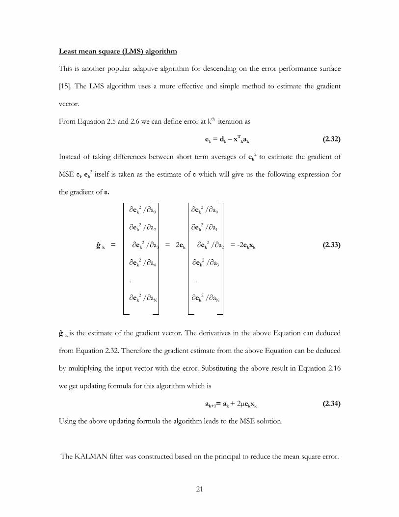
From Equation 2.5 and 2.6 we can define error at kth iteration as
ek = dk – xTkak (2.32)
Instead of taking differences between short term averages of ek2 to estimate the gradient of
MSE ε, ek2 itself is taken as the estimate of ε which will give us the following expression for
the gradient of ε.
∂ek2 /∂a0 ∂ek
2 /∂a0
∂ek2 /∂a2 ∂ek
2 /∂a1
ĝ k = ∂ek2 /∂a3 = 2ek ∂ek
2 /∂a2 = -2ekxk (2.33)
∂ek2 /∂a4 ∂ek
2 /∂a3
. .
∂ek2 /∂aN ∂ek
2 /∂aN
ĝ k is the estimate of the gradient vector. The derivatives in the above Equation can deduced
from Equation 2.32. Therefore the gradient estimate from the above Equation can be deduced
by multiplying the input vector with the error. Substituting the above result in Equation 2.16
we get updating formula for this algorithm which is
ak+1= ak + 2µekxk (2.34)
Using the above updating formula the algorithm leads to the MSE solution.
The KALMAN filter was constructed based on the principal to reduce the mean square error.
21

KALMAN Filter Derivation
In order to use the KALMAN filter on any signal, the process measured must be able to be
described by a linear dynamic system. The KALMAN filter has been developed using state
space techniques.
Consider a discrete time controlled process of a linear dynamic system that is governed by the
linear stochastic difference Equation.
gk+1=Agk+Buk+wk (2.35)
A linear difference Equation relates a variable to its previous values linearly as shown above.
Using this Equation a solution to gk+1 is found. g is the state variable of the system that
describes its dynamics. u is a known input that controls the system and B a constant matrix. A
is the state transition matrix that describes the changes in the state due to system dynamics. wk
is a random variable that represents the process noise.
The output of the system can be modeled as below [3]
yk=Hgk+vk (2.36)
H is the measurement matrix that relates the output of the system to the system state. yk is the
measured value or the output of the system. vk is the random variable that represent the
measurement noise.
The state variable g describes the system but this system state cannot be measured directly. So
we use the measured value y which is a function of g to obtain the best possible estimate of
the system state. A criterion [17] has to be employed while estimating the state g because the
measured value y cannot be trusted completely as it is corrupted by the measurement noise v.
22

The criteria for the estimator to determine the best estimate of the state, is to satisfy the
following two requirements. First the expected value of our state estimate should be equal to
the expected value of the true state. Second, the state estimate should vary as little as possible
from the true state which means that the estimator should have the error variance as low as
possible.
The KALMAN filter solution satisfies the above requirements when we make certain
assumptions about the noise that affects our system. The measured noise vk and the process
noise wk are assumed to be white noise, independent and have a normal probability
distribution. The covariance matrices of the process and measurement noise are denoted as Q
and R respectively and the error covariance matrix is denoted by P.[3]
Q = E {wkwkT} (2.37)
R = E {vkvkT} (2.38)
P = E {ekekT} (2.39)
ek is the estimation error (Equation 2.1). The above expressions can be deduced as follows.
Let us denote xi, xj to be two random variables. The covariance of the two random variables is
defined as
cov (xi, xj) = E{[xi – E(xi)] [xj – E(xj)]} (2.40)
if we consider the random variables to be white, zero mean, normal and independent then
E(xi) = 0 (2.41)
E(xj) = 0 (2.42)
E(xi), E(xj) represent the mean values of xi and xj which are equal to zero because the mean of
normal white random variables is zero.
Therefore,
23

cov (xi, xj) = E(xixj) (2.43)
Consider the case where i = j
cov (xi, xj) = E(xi2) (2.44)
If x is vector with random variables x1,….xn
cov (x, x) = E(x2) (2.45)
x2 = xxT (2.46)
Therefore,
cov (x, x) = E(xxT) (2.47)
From the above deduction we can conclude that the covariance matrices Q, R and P can be
expressed as shown in Equation 2.37, 2.38 and 2.39.
Based on the above assumptions a set of Equations are defined for the estimator. These
Equations are divided into two groups.
• Time Update Equations
ĝ k- = A ĝ k -1+Bu k -1 (2.48)
P k- = AP k -1A
T + Q (2.49)
• Measurement Update Equations
ĝ k = ĝ k-+Kk(yk -Hĝ k
-) (2.50)
Pk = (1 – KkH)Pk- (2.51)
Kk = Pk-HT(HPk
-HT+R)-1 (2.52)
ĝ k- is the a priori state estimate, ĝ k is the a posteriori state estimate, Pk
- is the a priori estimate
of the error covariance, Pk is the a posteriori estimate of the error covariance.
Pk- = E{ek
-ek-T} (2.53)
24
Pk = E{ekek
T} (2.54)
Kk is the KALMAN gain. yk is the measurement and Hĝ k- is the measurement prediction.
The origin of the filter is based on the following. We make a measurement yk. We also make a
prediction of this measurement using the a priori estimate ĝ k- which will be Hĝ k
-
(H is the matrix that relates the output of the system to the system state). (yk-- Hĝ k
-) is called
the residual or innovation [3]. It is the deviation of the predicted measurement from actual
measurement. Equation 2.48 from the set of Equations defined for the estimator predicts a
better estimate for the current state based on a linear combination of the a priori estimate ĝ k-
and a weighted version of the residual.
ĝ k = ĝ k-+Kk(yk
-- Hĝ k-)
The weight Kk (KALMAN gain) is chosen in such a way that it minimizes the a posteriori error
covariance Pk. From Equation 2.54 we have
Pk = E{ekek
T}
From Equation 2.1 we can rewrite Pk as
Pk = E{(gk - ĝk ) ( gk - ĝk)
T} (2.55)
Substituting Equation 2.50 in 2.55
Pk = E{[(1-KkH) (gk - ĝk-) – Kkvk] [(1-KkH) (gk - ĝk
-) – Kkvk]T} (2.56)
Taking the derivative of the trace from the above Equation with respect to K and equating it
to zero will give us value for K which will minimize the error covariance.
Kk = Pk-HT(HPk
-HT+R)-1
This is one of the measurement update Equations defined in the set of Equations for the
estimator (Equation 2.52).
Equation 2.56 can be expressed as [3]
25
Pk = (1-KkH)Pk-(1-KkH)T + KkRKk
T (2.57)
Substituting Equation 2.56 in 2.57 we get the measurement update Equation for the error
covariance (Equation 2.53).
Pk = (1 – KkH)Pk-
The time update Equation for the error covariance can be deduced as following.
ek+1- = gk+1 - ĝk+1
- (2.58)
Equation 2.58 represents the error in our a priori estimate.
State projection is done as
ĝ k- = Aĝ k -1 (2.59)
where ĝ k- is the a priori state estimate and ĝ k -1 is the previous a posteriori state estimate.
Based on Equation 2.59 and 2.35
ek+1- = (Agk+wk) – (Aĝ k) (2.60)
Rearranging Equation 2.60
ek+1- = A(gk -ĝ k) + wk (2.61)
Based on Equation 2.1 we can express Equation 2.61 as
ek+1- = (Aek+wk) (2.62)
From Equation 2.53 we can express the a priori error covariance as
Pk+1- = E{(ek+1
-)( ek+1-)T} (2.63)
Substituting Equation 2.62 in 2.63 we get
Pk+1- = E{(Aek+wk) (Aek+wk)
T} (2.64)
The cross correlation between wk and ek will be zero [3]. Therefore
Pk+1- = E{(Aek)( Aek)
T} + E {wkwkT} (2.65)
Equation 2.65 can be rearranged as
Pk+1- = AE{ekek
T}AT + E {wkwkT} (2.66)
26
Based on Equations 2.37 and 2.39
P k+1- = AP k A
T + Q (2.67)
From the above Equation we can express the time update Equation for error covariance
as shown in Equation 2.51
P k- = AP k-1 A
T + Q
Filter Algorithm
Figure 2.3 shows the block diagram of the steps required in implementing the KALMAN
filter. Initially a posteriori state ĝk and a posteriori error covariance P k are assigned a guess
value. These values are used to predict forward in time the a priori state ĝk+1- and the a priori
error covariance P k+1- based on Equations 2.45 and 2.46. The estimation of the measurement
is given by the product of a priori state ĝk+1- and measurement matrix H as shown in the
Figure 2.3. The error in our estimation can be obtained. This error which is also called the
residual is substituted in Equation 2.47 to obtain updated a posteriori state ĝk+1 which will be
again used in the next cycle of prediction. KALMAN gain Kk which was a part of Equation
2.47 is calculated based on the a priori error covariance P k+1- predicted in the first step. It is
here that the actual error minimization takes place because the KALMAN gain is calculated
based on the principal to reduce the error covariance. The expression for KALMAN gain is
given in Equation 2.49. An updated a posteriori error covariance P k+1 is calculated based on
Equation 2.48 and this value will be used in the next iteration for predicting the a priori error
covariance. KALMAN gain adjusts its value for every iteration and slowly converges to an
optimal value such that the error covariance reaches its minimum.
27
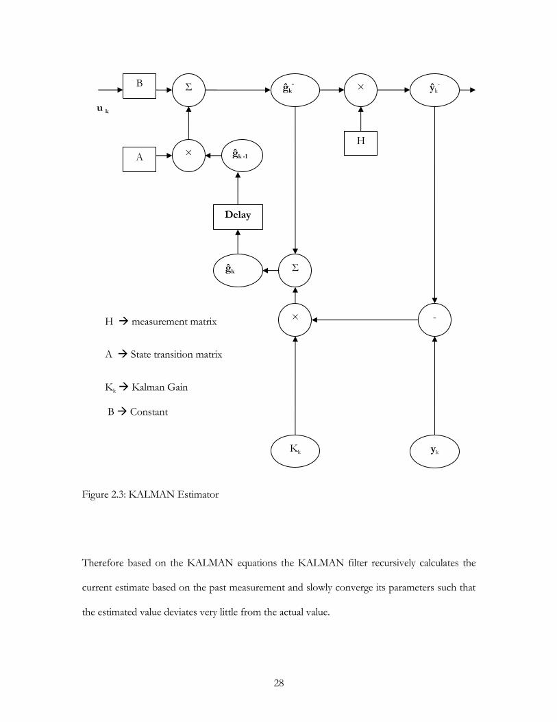
Figure 2.3: KALMAN Estimator
Therefore based on the KALMAN equations the KALMAN filter recursively calculates the
current estimate based on the past measurement and slowly converge its parameters such that
the estimated value deviates very little from the actual value.
B Σ
A ×
ĝk- × ŷk
-
H
-
yk
×
Σĝk
Delay
ĝk -1
u k
H measurement matrix
A State transition matrix
Kk Kalman Gain
B Constant
Kk
28

Chapter 3 discusses one implementation of the KALMAN filter used to estimate the ECG RR
interval.
29
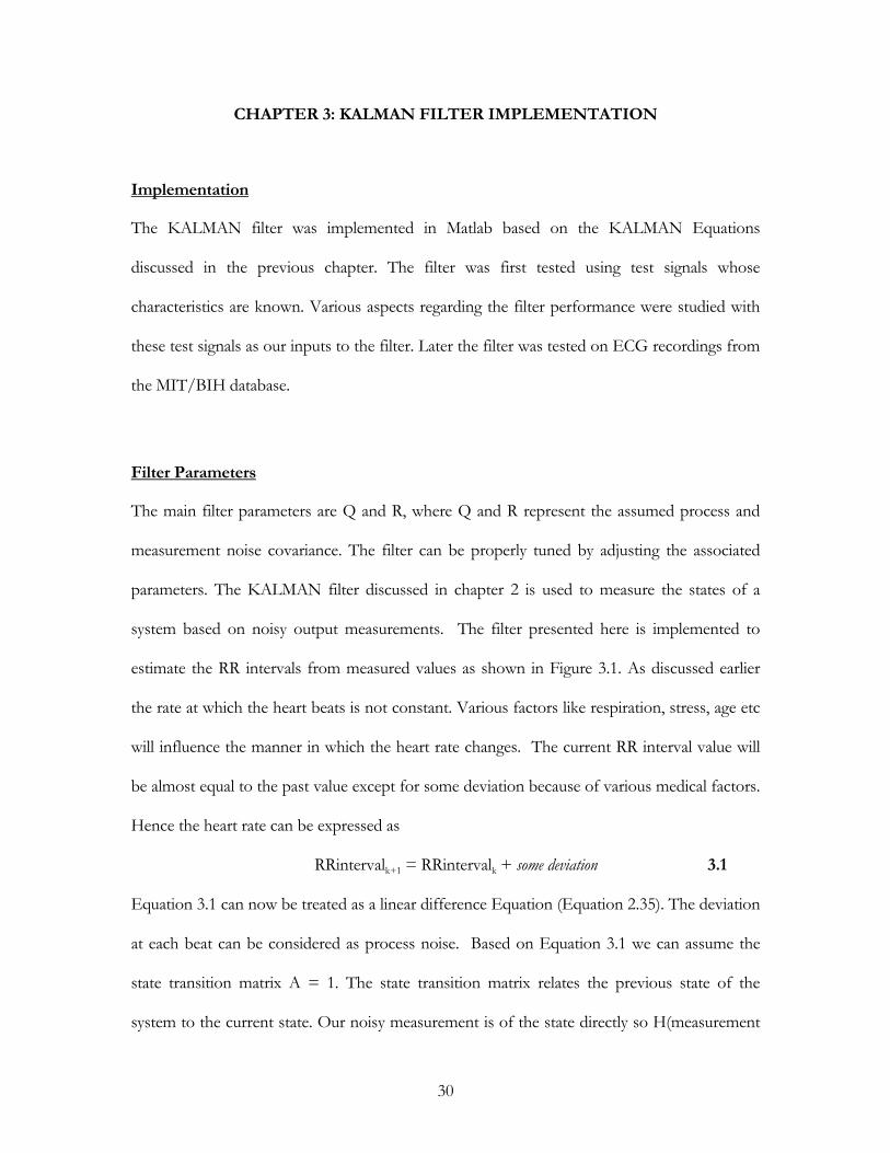
CHAPTER 3: KALMAN FILTER IMPLEMENTATION
Implementation
The KALMAN filter was implemented in Matlab based on the KALMAN Equations
discussed in the previous chapter. The filter was first tested using test signals whose
characteristics are known. Various aspects regarding the filter performance were studied with
these test signals as our inputs to the filter. Later the filter was tested on ECG recordings from
the MIT/BIH database.
Filter Parameters
The main filter parameters are Q and R, where Q and R represent the assumed process and
measurement noise covariance. The filter can be properly tuned by adjusting the associated
parameters. The KALMAN filter discussed in chapter 2 is used to measure the states of a
system based on noisy output measurements. The filter presented here is implemented to
estimate the RR intervals from measured values as shown in Figure 3.1. As discussed earlier
the rate at which the heart beats is not constant. Various factors like respiration, stress, age etc
will influence the manner in which the heart rate changes. The current RR interval value will
be almost equal to the past value except for some deviation because of various medical factors.
Hence the heart rate can be expressed as
RRintervalk+1 = RRintervalk + some deviation 3.1
Equation 3.1 can now be treated as a linear difference Equation (Equation 2.35). The deviation
at each beat can be considered as process noise. Based on Equation 3.1 we can assume the
state transition matrix A = 1. The state transition matrix relates the previous state of the
system to the current state. Our noisy measurement is of the state directly so H(measurement
30

matrix) = 1. Some guess values are taken for the apriori state and apriori error covariance. The
filter will eventually converge irrespective of the guess values.
Filter adaptation
Figure 3.1 briefly outlines the procedure to test the filter adaptation. A test signal is generated
which will serve as our filter input. As the QRS detector will produce an impulse train by
detecting and placing an impulse wherever a QRS complex occurs in the ECG and the
intervals between them will be the RR interval, it would be appropriate for us to select an
impulse train as our test signal. The intervals between the impulses in our test signal were
varied according to a known pattern as shown in Figure 3.2. The RR intervals are measured.
These varying RR intervals are shown in Figure 3.3. The measured intervals were then passed
through our filter for it to estimate the time interval. The estimated intervals were then
compared to the measured intervals. Because of our prior knowledge of the nature of the
interval variation we can best describe the filter performance from its estimated values. From
the output of the filter as shown in Figure 3.4 we can observe the rate at which the filter adapts
itself to best estimate from the measured data. The comparison is better seen in Figure 3.5.
This shows us that the filter implemented here can adapt to any time interval and it is a desired
feature because the heart rates vary from one person to other and the filter should adapt to
those changes.
31

Generate the test signal
Intervals of the test signal are
measured
Define the filter
parameters
Based on the parameters and the input intervals the KALMAN filter Equations are used to compute the estimated intervals
Estimated intervals
Measured intervals
The error in the estimation is computed and sent as a feedback to the filter for
optimization
Figure 3.1: KALMAN Filter Implementation on the test signal
32
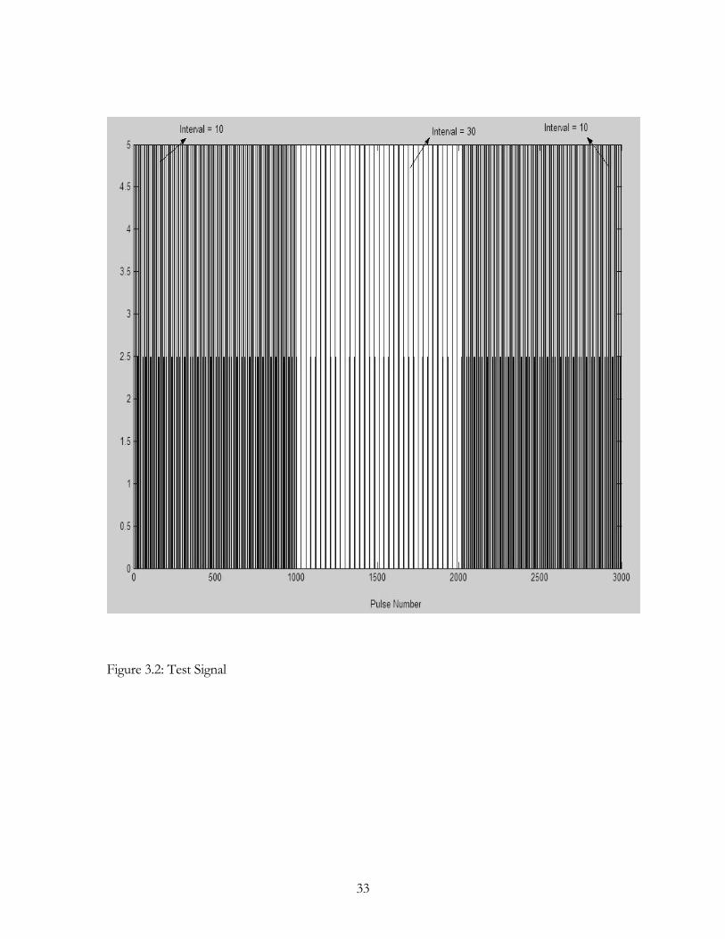
Figure 3.2: Test Signal
33

Figure 3.3: Intervals of the test signal
Figure 3.4: Estimated Interval
34

Figure 3.5: Comparison of the estimated interval with actual interval
The estimation error is plotted and shown in Figure 3.6. We can see that the error shoots up
when there is a drastic change in the input interval but it quickly drops back as the filter learns
the change. It can be shown that the KALMAN gain converges to an optimum value from the
plot shown in Figure 3.7.
35
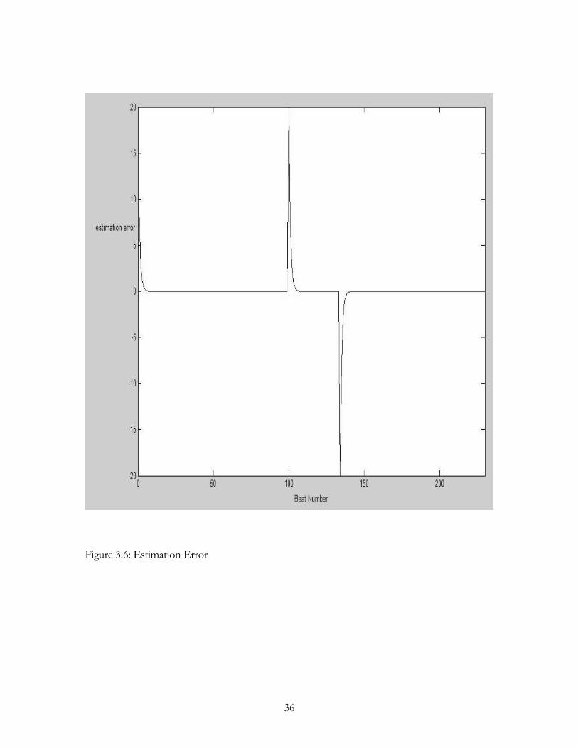
Figure 3.6: Estimation Error
36

Figure 3.7: KALMAN Gain
Performance in noisy environment
The input in the previous section was noise free. There is always a possibility to make errors
while measuring the intervals. This noise is called as the measurement noise. Instead of a clean
37

input, we feed the filter with a noise corrupted input. Usually the measurement noises tend to
be Gaussian by nature, so we corrupt the input intervals with Gaussian noise. Now we have
noisy interval measurements as our filter input. The filter performance is studied by observing
the estimated values from the filter output. The filter output is compared to the noisy input
and the actual input as shown in Figure 3.8.
Figure 3.8: Performance of the filter with a noisy input
From the comparison in Figure 3.8 we can observe that the estimated values are closer to the
actual values than the measured values which are corrupted with noise. Therefore the
KALMAN filter will reduce the noise that will cause our measurements to deviate from the
actual values.
38
Filter performance with different parameters
The filter parameters were varied and its performance on various aspects has been observed.
First the filter was tested on our noise corrupted signal for different assumptions of the
measurement noise. The plots are shown in Figure 3.9. It is shown from the estimated values
that the filter estimates follow closely the noisy measurements when the assumed measurement
covariance is a low value (here V = 0.5). But if the measurement noise covariance is
considered to be high the filter estimates were slower in following the measurements and that’s
the reason why the output deviates a lot from the actual interval.
The effect on the performance of the filter by varying the filter parameters was also studied on
our noise free test signal (Figure 3.2). The measurement noise covariance is varied through a
range of values and the absolute mean estimation error for each value was observed and
plotted as shown in Figure 3.10 and as expected we see that the mean estimation error
increases with the increase in the measurement noise covariance.
39
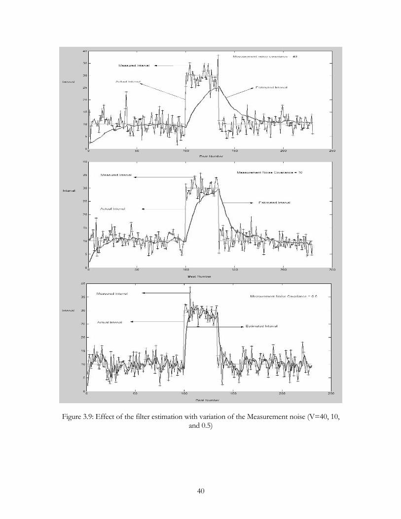
Figure 3.9: Effect of the filter estimation with variation of the Measurement noise (V=40, 10, and 0.5)
40
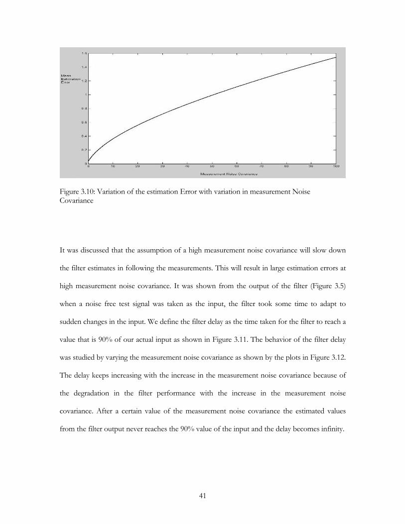
Figure 3.10: Variation of the estimation Error with variation in measurement Noise Covariance
It was discussed that the assumption of a high measurement noise covariance will slow down
the filter estimates in following the measurements. This will result in large estimation errors at
high measurement noise covariance. It was shown from the output of the filter (Figure 3.5)
when a noise free test signal was taken as the input, the filter took some time to adapt to
sudden changes in the input. We define the filter delay as the time taken for the filter to reach a
value that is 90% of our actual input as shown in Figure 3.11. The behavior of the filter delay
was studied by varying the measurement noise covariance as shown by the plots in Figure 3.12.
The delay keeps increasing with the increase in the measurement noise covariance because of
the degradation in the filter performance with the increase in the measurement noise
covariance. After a certain value of the measurement noise covariance the estimated values
from the filter output never reaches the 90% value of the input and the delay becomes infinity.
41

Figure 3.11: Defining the filter delay
This can be justified from our previous discussion that a high measurement noise covariance
increases filter estimates. This behavior can be shown from the plot shown in Figure 3.12.
Figure 3.12: Variation of the filter delay with variation in Measurement Noise Covariance
42

All the previous results were also obtained by varying the process noise covariance. The results
of the filter performance in the presence of noise, absolute mean estimation error and the time
delay is shown in figures 3.13 – 3.15.
By assuming a high process noise covariance (Q) it can be shown in Figure 3.13 that the filter
estimates follow the measurements very closely.
Figure 3.13: Filter performance with the process noise covariance assumed to be 10
While assuming high uncertainty (high Q) in the process it is desirable to have process
measurements that are reliable because the filter will assume a high process noise covariance
43
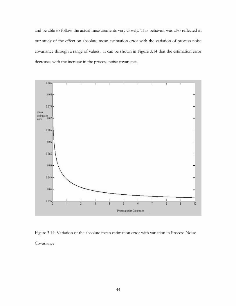
and be able to follow the actual measurements very closely. This behavior was also reflected in
our study of the effect on absolute mean estimation error with the variation of process noise
covariance through a range of values. It can be shown in Figure 3.14 that the estimation error
decreases with the increase in the process noise covariance.
Figure 3.14: Variation of the absolute mean estimation error with variation in Process Noise
Covariance
44

This can be justified from our discussion that when the filter assumes a high process noise
covariance it will be able to follow the actual measurements very closely and hence the
estimation error would obviously be less. It is exactly the opposite when we vary the
measurement noise covariance (Figure 3.12) where the estimation error increases with an
increase in the measurement noise covariance because when the filter assumes high
measurement noise covariance it will not be able to follow the actual measurements closely.
Figure 3.15 shows the behavior of the filter delay with the variation of the process noise
covariance.
Figure 3.15: Variation of the filter delay with variation in the Process Noise Covariance
45

The filter delay decreases with the increase in the process noise covariance because the filter
estimates follow the measurements very closely when the process noise covariance was
assumed to be high and any change in the filter input, the filter will quickly learn them.
When it comes to the practical implementation of the filter, the measurement noise covariance
(R) can be known before hand. It can be determined by taking few offline sample
measurements. It is difficult to have an accurate value of the process noise covariance (Q) as
we cannot directly observe the process we are estimating. However superior filter performance
can be obtained by properly tuning the filter parameters Q and R though we do not have a
rational basis in choosing them.
Statistics
The values for the measured intervals, estimated intervals from the filter output and the actual
intervals for the plot shown in Figure 3.8 is listed through tables A1 to A7 in appendix. The
average and standard deviation of the measured intervals and estimated intervals shown in
Table 3.1 are computed from this simulated data.
Table 3.1: Statistics of measured and estimated RR intervals
Average of actual intervals 12.95652
Average of measured intervals 13.11652
Average of estimated intervals 13.00651
Standard Deviation of measured intervals 7.953382
Standard Deviation of estimated intervals 6.855498
Standard Deviation of actual intervals 7.114032
46

From the statistics in Table 3.1 it is shown that filter was able to estimate the intervals close to
the actual intervals, from the interval measurements which deviate from the actual intervals
due to the addition of measurement noise.
As shown in Table A1 the filter started out with an initial guess value of 2 for the interval. The
actual interval was 10. The filter took just seven iterations to reach an estimated value of 10.05
which is indeed very close to the actual interval. As shown in Table A3 at the 100th beat the
actual interval changes from 10 to 30. It is shown that the filter took nine iterations to reach an
estimated value of 30.579. And at 134th beat (Table A4) when the actual interval dropped back
to 10 it took eleven iterations for the filter to estimate a value of 10.127 (Table A5). The filter
was quick in learning in spite of a large variance in the input.
47
CHAPTER 4: IMPLEMENTATION ON ECG RECORDINGS
Implementation setup
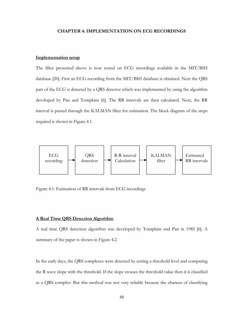
The filter presented above is now tested on ECG recordings available in the MIT/BIH
database [20]. First an ECG recording from the MIT/BIH database is obtained. Next the QRS
part of the ECG is detected by a QRS detector which was implemented by using the algorithm
developed by Pan and Tompkins [6]. The RR intervals are then calculated. Next, the RR
interval is passed through the KALMAN filter for estimation. The block diagram of the steps
required is shown in Figure 4.1.
Figure 4.1: Estimation of RR intervals from ECG recordings
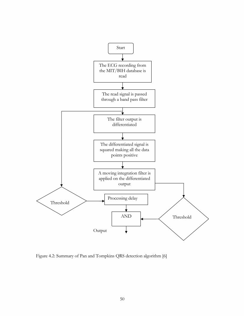
A Real Time QRS Detection Algorithm
A real time QRS detection algorithm was developed by Tompkins and Pan in 1985 [6]. A
summary of the paper is shown in Figure 4.2.
In the early days, the QRS complexes were detected by setting a threshold level and comparing
the R wave slope with the threshold. If the slope crosses the threshold value then it is classified
as a QRS complex. But this method was not very reliable because the chances of classifying
ECG
recording QRS
detection R-R interval Calculation
KALMAN filter
Estimated RR intervals
48

noise peaks as QRS complexes were very high. The method developed by Dr. Tompkins takes
into consideration other parameters of the signal such as the signal amplitude and the width of
the QRS to determine if a signal peak is QRS complex or not.
First the ECG signal is passed through a band pass filter to remove noises like the muscle
lope
oth the classifications made by using the band pass filter and integrator outputs are AND ed
he QRS detector output will be an impulse train with the impulses located wherever the
noise, 60HZ interference, baseline wander and T-wave interference. An adaptive threshold is
used on this filter output to determine the QRS complexes based on the signal amplitude.
This filtered output is then passed through a differentiator to obtain the QRS complex s
information. The output of the differentiator is then squared to make all the data points
positive and also emphasize the high frequencies which are usually the QRS components.
Then the squared signal is passed through a moving window integrator to extract out the
width of the QRS complex. The duration of the rising edge of the integration waveform gives
the width of the QRS complex. Therefore the rising edge of the integrator output waveform
can be used to find a QRS complex. An adaptive threshold is applied on this output to classify
the QRS complex.
B
together to give out the final output.
T
detector locates a QRS complex. The RR intervals can now be computed from this impulse
train and passed through the KALMAN filter for estimation.
49
Start
The ECG recording from the MIT/BIH database is
read
The read signal is passed through a band pass filter
The filter output is differentiated
The differentiated signal is squared making all the data
points positive
A moving integration filter is applied on the differentiated
output
Figure 4.2: Summary of Pan and Tompkins QRS detection algorithm [6]
Processing delay Threshold
AND Threshold
Output
50

Results for real ECG data
The KALMAN filter was tested on 10 ECG recordings and the results are shown through
Figures 4.3 to 4.24. Based on the quality of the QRS detection signal the filter was tuned by
varying its parameters to best estimate the RR interval and as well filter out any measurement
noise. The criteria for the parameters was to select high R (measurement noise covariance)
value if the detector output is erratic and low R value if the detector accurately classifies the
QRS complexes.
If the RR intervals are measured from an erroneous QRS detector output, it is obvious that
there will be errors in the interval measurements. Because of these errors the interval
measurements deviate widely from the actual intervals. From our discussion in chapter 3 it has
been shown that the assumption of high R (measurement noise covariance) will slow down the
filter estimates in following the measurements. Therefore the interval measurements are less
trusted and the filter will tend to estimate values that do not vary as widely as the
measurements. Thus the filter estimates would be more close to the actual values. This leads us
to tune the parameter R to high values if the QRS detector output is erroneous.
If the QRS detection was accurate a very low value for R and a high value for Q were
assumed. If the QRS detection was accurate then there would be a very less chance for the RR
interval measurements to be erroneous. From our discussion in chapter 3 we determined how
the filter behaved for low values of R and for high values of Q. By assuming high Q, the filter
estimates follow the measurements very closely. Since our measurements here have fewer
errors, this is a desired feature. Additionally a very low value for R will also make the filter
follow the measurements more quickly.
51

Therefore based on the performance of the QRS detector on the ECG signals, appropriate
values for Q and R have been assumed. Table 4.2 lists the parameters chosen for different
ECG signals from the MIT/BIH database [20].
Table 4.1: Filter parameters for the ECG recordings
MIT/BIH (database)
file name
Process Noise Covariance
(Q)
Measurement Noise Covariance
( R )
100.dat 3 20.0
101.dat 4 15.0
102.dat 5 0.1
103.dat 4 10.0
104.dat 4 1.0
105.dat 4 12.0
106.dat 4 12.0
107.dat 4 0.1
118.dat 4 15.0
119.dat 5 20.0
52

Figure 4.3: ECG and the QRS detector plot for file 100.dat
53

Figure 4.4: Measured Intervals and Estimated intervals for file 100.dat
The RR interval should be fluctuating somewhere around 0.8 seconds. But because of bad
performance of the QRS detection (Figure 4.3) it is shown in Figure 4.4 there are a few noise
pulses in the RR interval measurements. This is because of the failure of the QRS detector to
detect all the QRS complexes in the ECG signal. Missed beats caused the noise pulses in our
RR interval measurement. So a selection of high R would cause less deviation in our estimated
values. Here R was assumed a value of 20 and Q a value of 3. It can be shown that the
estimated values are still closer to our heart rate (0.8 seconds) than RR interval measurements.
54
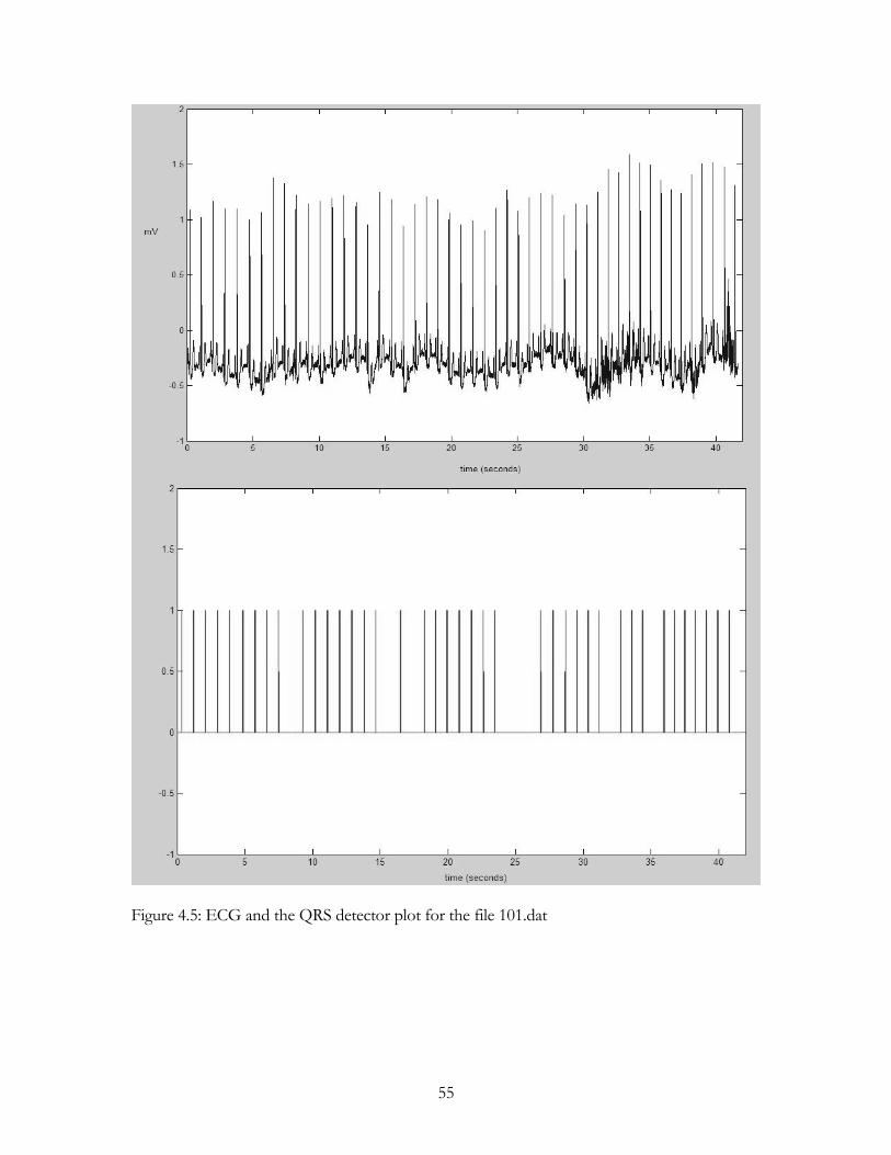
Figure 4.5: ECG and the QRS detector plot for the file 101.dat
55
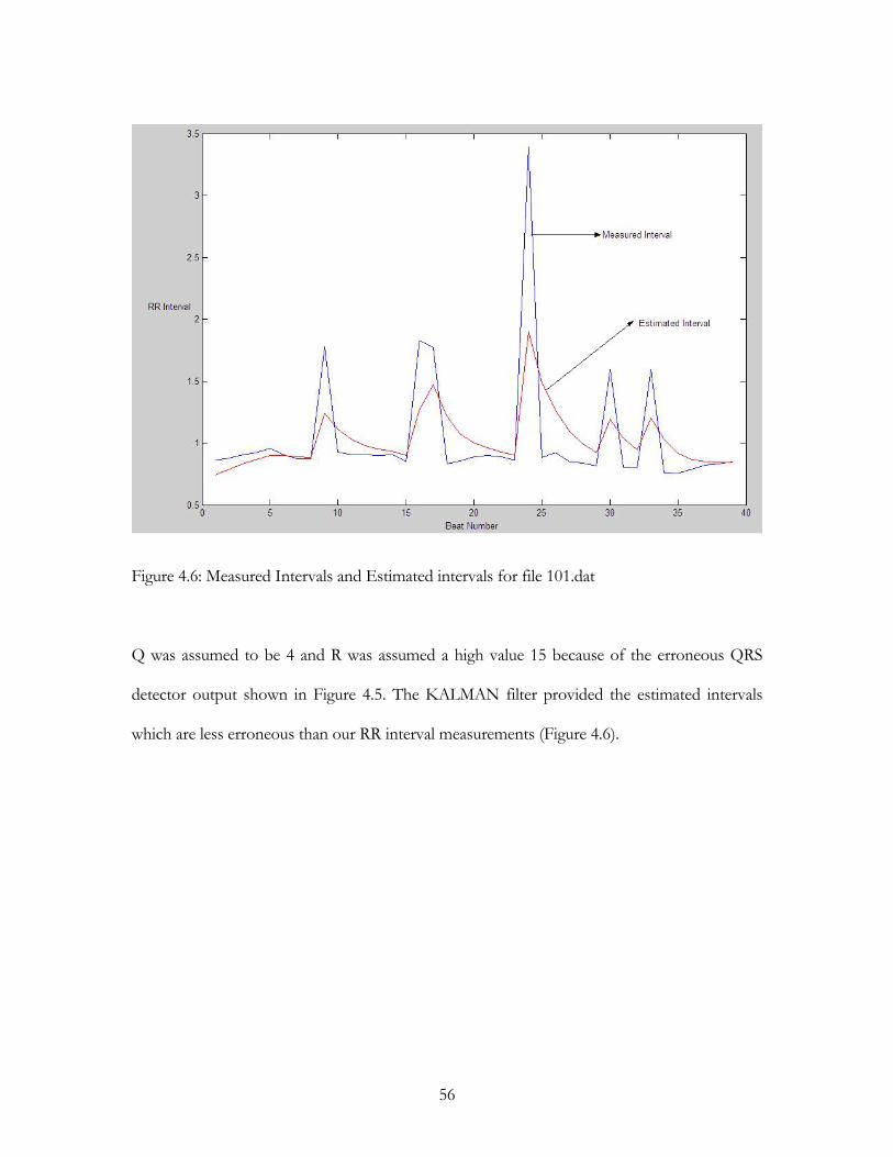
Figure 4.6: Measured Intervals and Estimated intervals for file 101.dat
Q was assumed to be 4 and R was assumed a high value 15 because of the erroneous QRS
detector output shown in Figure 4.5. The KALMAN filter provided the estimated intervals
which are less erroneous than our RR interval measurements (Figure 4.6).
56

Figure 4.7: ECG and QRS detector plots for file 102.dat
57

Figure 4.8: Measured Intervals and Estimated intervals for file 102.dat
It is shown in Figure 4.7 that the QRS detector output was very accurate which leads us to
assume a very low value for R (0.1) and relatively higher value for Q (5). Figure 4.8 shows the
estimated values of the filter which follow our RR interval measurements very closely. Since
the measurements have no errors they can be considered as the actual intervals and the
KALMAN filter was able to estimate them accurately.
58
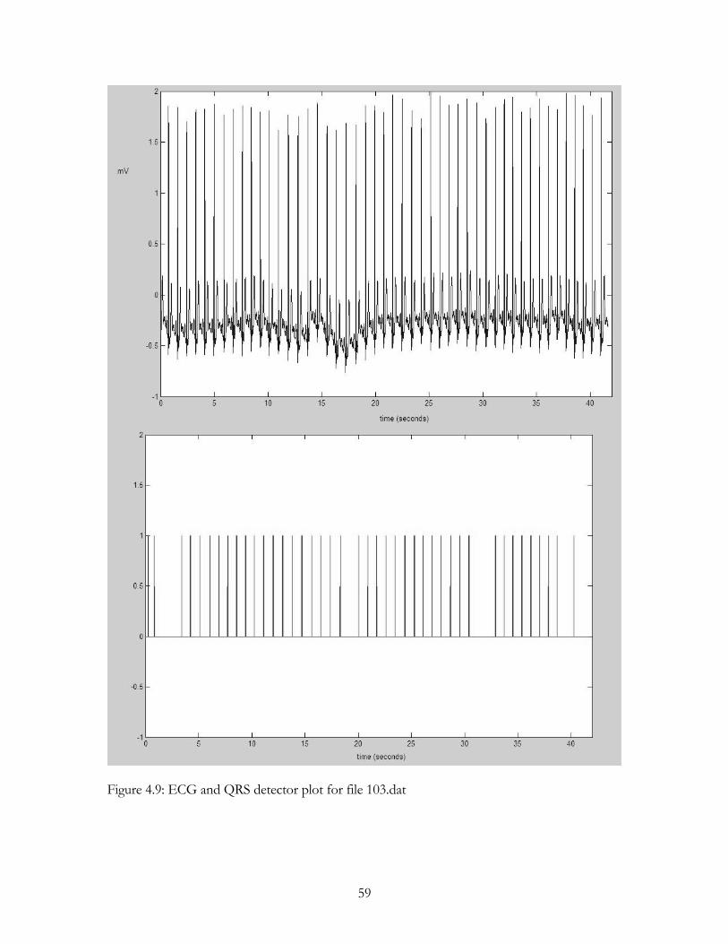
Figure 4.9: ECG and QRS detector plot for file 103.dat
59

Figure 4.10: Measured Intervals and Estimated intervals for file 103.dat
Figure 4.9 show that the QRS detector misses many beats in the ECG. When the RR interval
is computed, it is shown in Figure 4.10 that the extended interval resulted in noise pulses at
instances where the QRS detector missed a beat. The filter estimation shows that the estimated
intervals are kept low at the occurrence of the noise pulses thus decreasing the error.
60
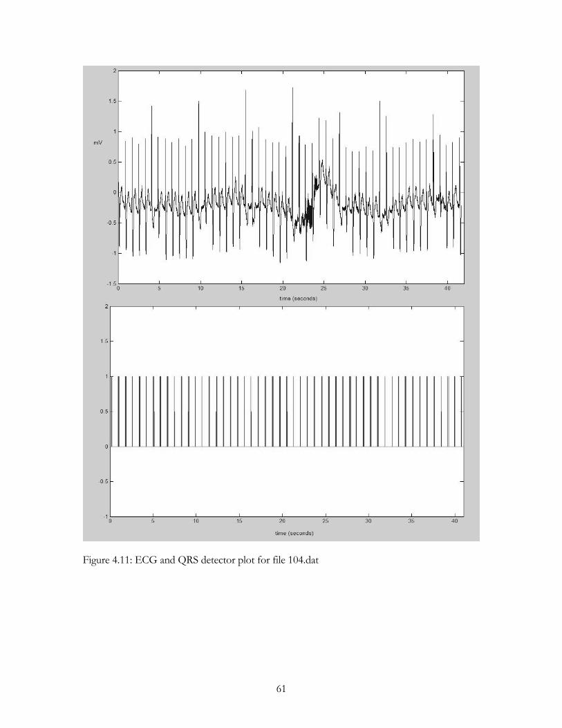
Figure 4.11: ECG and QRS detector plot for file 104.dat
61

Figure 4.12: Measured Intervals and Estimated intervals for file 104.dat
Here the parameter R was chosen a low value of 1 because the QRS detection was accurate
thus giving us less erroneous RR intervals. Q was assigned a value of 4. As shown in Figure
4.12 the filter was able to estimate the intervals from the given RR interval measurements.
Since the measurements didn't have any errors, our filter estimation was close to the
measurements as shown in Figure 4.12.
62

Figure 4.13: ECG and QRS detector plot for file 105.dat
63
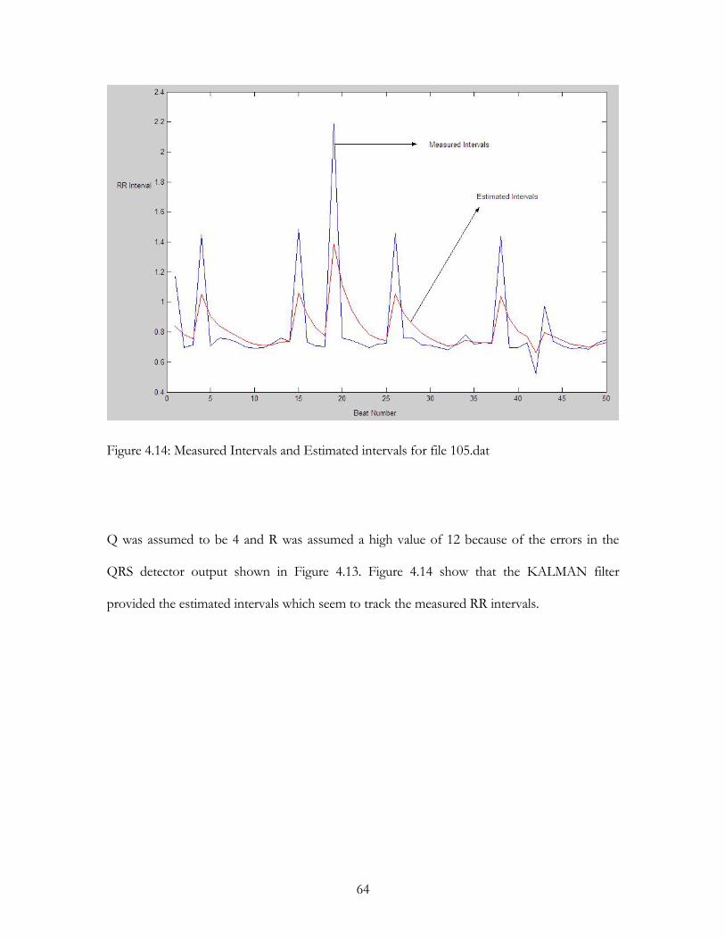
Figure 4.14: Measured Intervals and Estimated intervals for file 105.dat
Q was assumed to be 4 and R was assumed a high value of 12 because of the errors in the
QRS detector output shown in Figure 4.13. Figure 4.14 show that the KALMAN filter
provided the estimated intervals which seem to track the measured RR intervals.
64
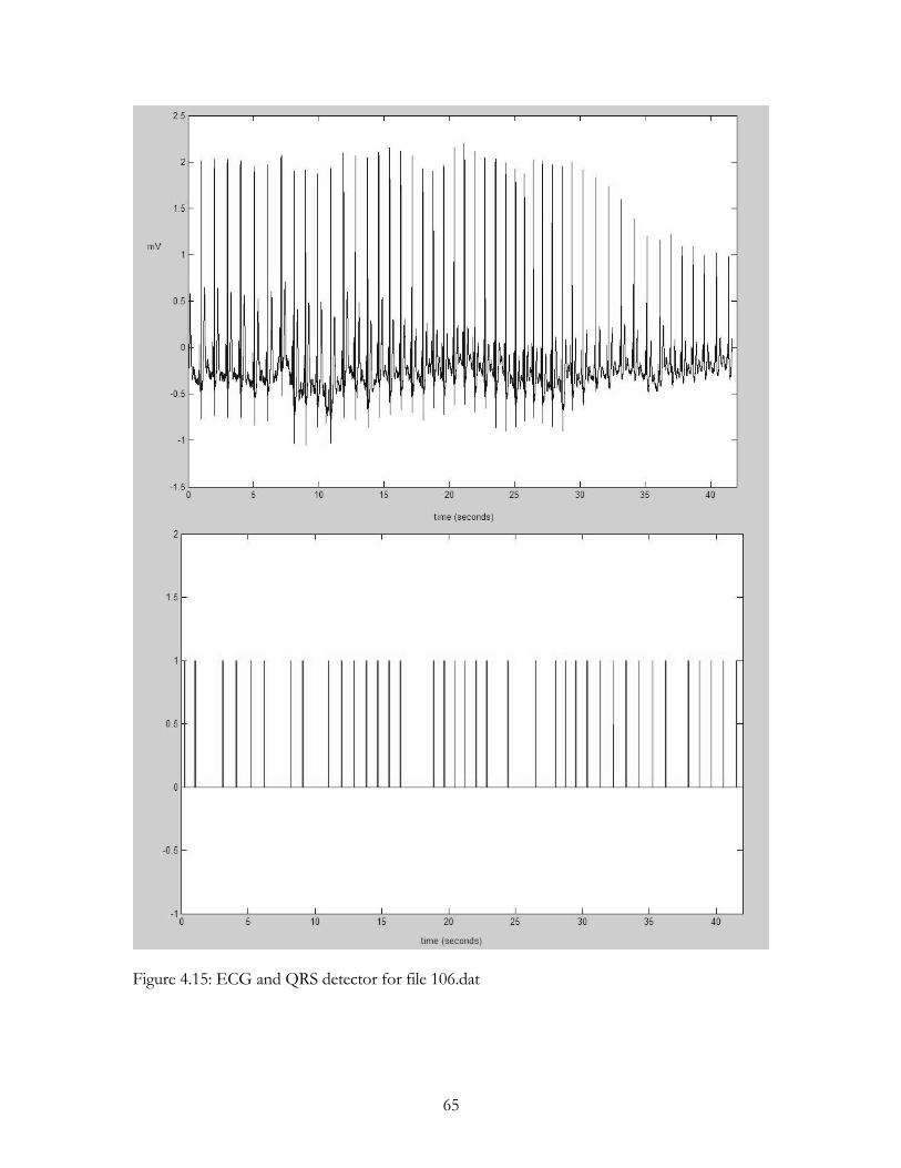
Figure 4.15: ECG and QRS detector for file 106.dat
65

Figure 4.16: Measured Intervals and Estimated intervals for file 106.dat
Q was assumed to be 4 and R was assumed a high value 12 because of the errors in the QRS
detector output shown in Figure 4.15. Figure 4.16 show that the KALMAN filter provided the
estimated intervals which tracked the RR interval measurements.
66
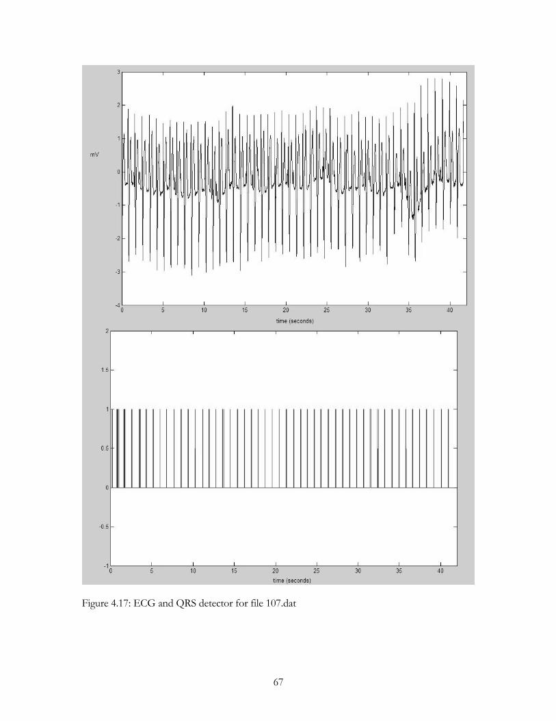
Figure 4.17: ECG and QRS detector for file 107.dat
67

Figure 4.18: Measured Intervals and Estimated intervals for file 107.dat
As shown in Figure 4.17, the QRS detector output was very accurate which leads us to assume
a very low value for R (0.1) and relatively higher value for Q (4). Figure 4.18 shows the
estimated values of the filter which follow our measured RR intervals very closely. Since the
QRS detection has no errors, the measured RR interval and the KALMAN filter estimation
had good agreement.
68

Figure 4.19: ECG and QRS detector plot for file 118.dat
69
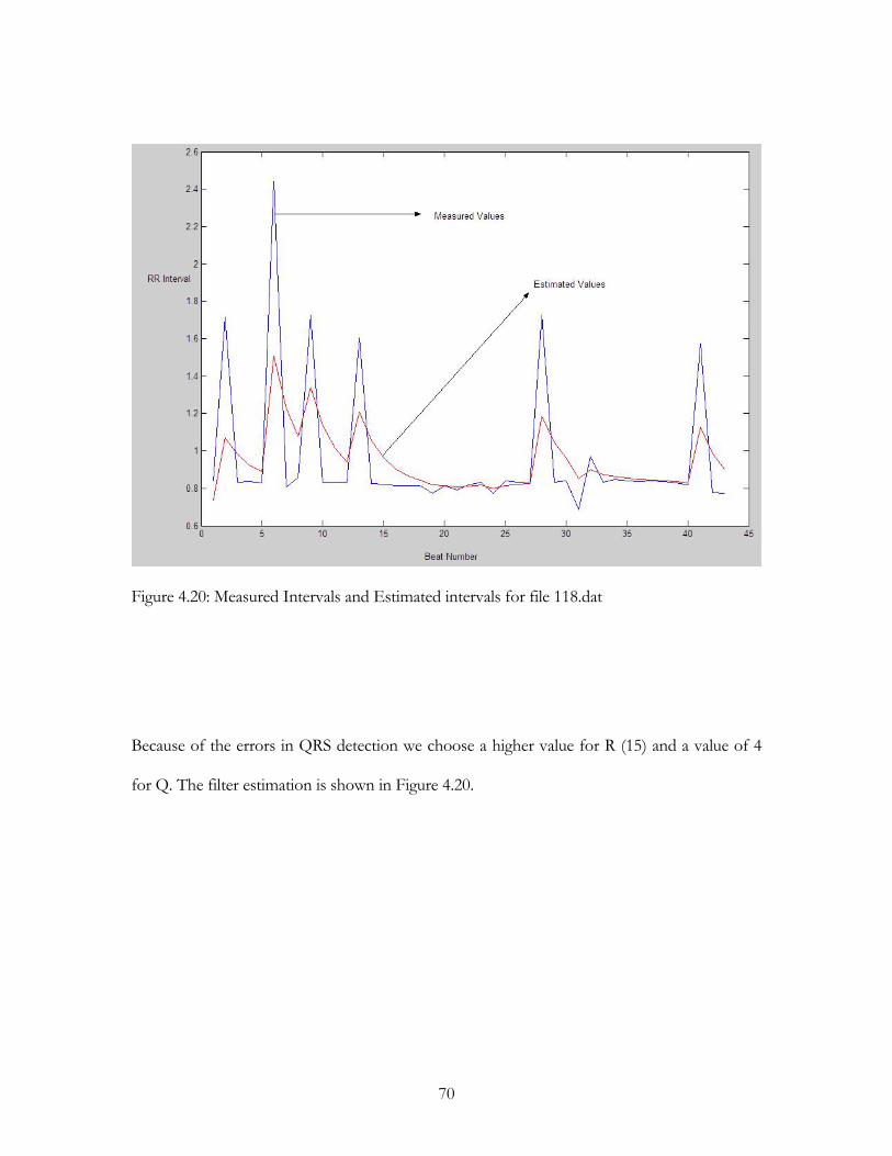
Figure 4.20: Measured Intervals and Estimated intervals for file 118.dat
Because of the errors in QRS detection we choose a higher value for R (15) and a value of 4
for Q. The filter estimation is shown in Figure 4.20.
70
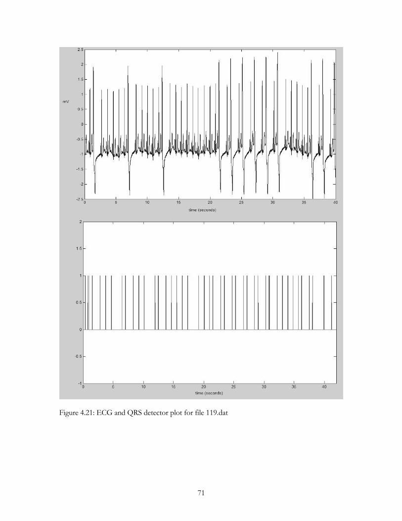
Figure 4.21: ECG and QRS detector plot for file 119.dat
71

Figure 4.22: Measured Intervals and Estimated intervals for file 119.dat
Q was assumed to be 5 and R was assumed a high value of 20 because of the errors in the
QRS detector output as shown in Figure 4.21. Figure 4.22 shows that the KALMAN filter
provided the estimated intervals that is in close agreement with the actual RR interval values.
Therefore from the results it was shown that KALMAN filter was able to estimate the RR
intervals that are in close agreement to the actual intervals, by appropriate selection of the filter
parameters.
72
CONCLUSION AND FUTURE WORK
Conclusion
Development of a KALMAN filter based estimation algorithm to estimate the RR intervals
was the main contribution of this thesis. We considered an impulse train as the input to the
KALMAN filter. The intervals between the impulses were estimated using the filter presented
here. We were able to study the performance of the filter on this impulse train because of our
prior knowledge of the intervals between the impulses. The filter was able to estimate the
intervals with good accuracy. The filter was then tested on the same impulse train but the
intervals between the impulses were now corrupted with Gaussian random noise. The filter
was able estimate the RR intervals whose values were closer to the actual intervals than the
noise corrupted intervals.
The KALMAN filter was then implemented on ECG recordings available in the MIT/BIH
database. A QRS detection algorithm was applied on the ECG recordings to detect the QRS
complexes. The RR intervals were computed from this detector output. Since the performance
of the detector varied from one ECG recording to another, the RR intervals computed had
noise spikes due to missed beats. The filter was able to reduce these errors and estimate the
RR intervals close to the actual values.
73

Future Work
• A linear KALMAN filter was used in this thesis for estimation because the process
here was taken to be a linear model. We can assume a non linear model for our
process and use an Extended KALMAN filter for the estimation.
• Since the KALMAN filter implemented here is based on a discrete algorithm, it is well
suited to be implemented on a DSP board. The actual performance and the theoretical
performance can then be compared.
74

APPENDIX A
SIMULATED DATA
75
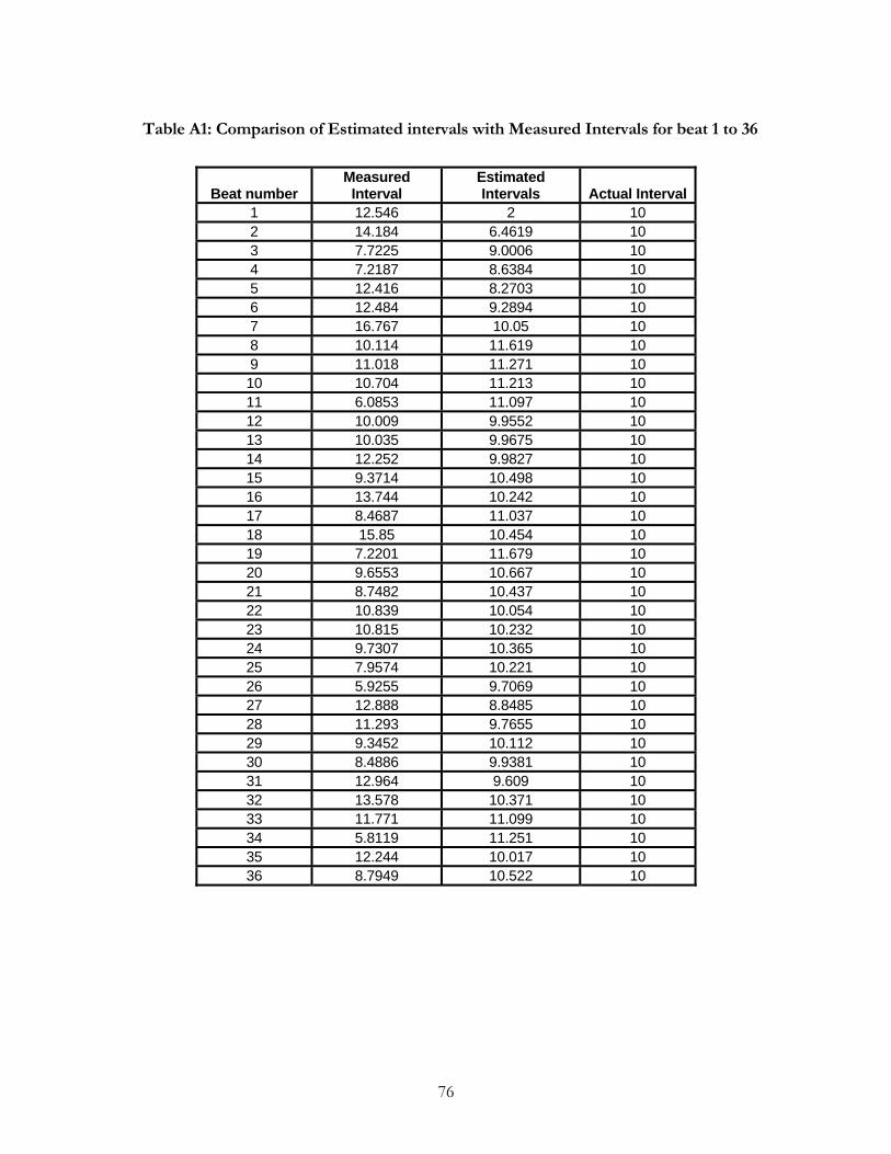
Table A1: Comparison of Estimated intervals with Measured Intervals for beat 1 to 36
Beat number Measured
Interval Estimated Intervals Actual Interval
1 12.546 2 10 2 14.184 6.4619 10 3 7.7225 9.0006 10 4 7.2187 8.6384 10 5 12.416 8.2703 10 6 12.484 9.2894 10 7 16.767 10.05 10 8 10.114 11.619 10 9 11.018 11.271 10 10 10.704 11.213 10 11 6.0853 11.097 10 12 10.009 9.9552 10 13 10.035 9.9675 10 14 12.252 9.9827 10 15 9.3714 10.498 10 16 13.744 10.242 10 17 8.4687 11.037 10 18 15.85 10.454 10 19 7.2201 11.679 10 20 9.6553 10.667 10 21 8.7482 10.437 10 22 10.839 10.054 10 23 10.815 10.232 10 24 9.7307 10.365 10 25 7.9574 10.221 10 26 5.9255 9.7069 10 27 12.888 8.8485 10 28 11.293 9.7655 10 29 9.3452 10.112 10 30 8.4886 9.9381 10 31 12.964 9.609 10 32 13.578 10.371 10 33 11.771 11.099 10 34 5.8119 11.251 10 35 12.244 10.017 10 36 8.7949 10.522 10
76
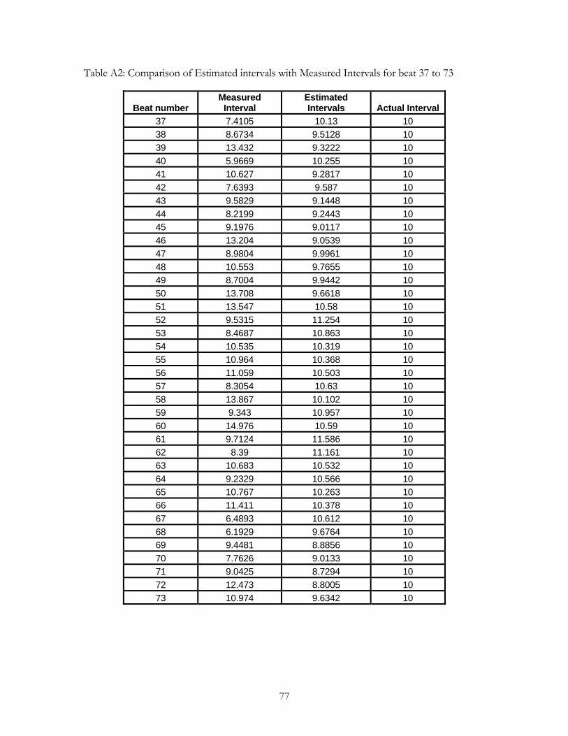
Table A2: Comparison of Estimated intervals with Measured Intervals for beat 37 to 73
Beat number Measured
Interval Estimated Intervals Actual Interval
37 7.4105 10.13 10 38 8.6734 9.5128 10 39 13.432 9.3222 10 40 5.9669 10.255 10 41 10.627 9.2817 10 42 7.6393 9.587 10 43 9.5829 9.1448 10 44 8.2199 9.2443 10 45 9.1976 9.0117 10 46 13.204 9.0539 10 47 8.9804 9.9961 10 48 10.553 9.7655 10 49 8.7004 9.9442 10 50 13.708 9.6618 10 51 13.547 10.58 10 52 9.5315 11.254 10 53 8.4687 10.863 10 54 10.535 10.319 10 55 10.964 10.368 10 56 11.059 10.503 10 57 8.3054 10.63 10 58 13.867 10.102 10 59 9.343 10.957 10 60 14.976 10.59 10 61 9.7124 11.586 10 62 8.39 11.161 10 63 10.683 10.532 10 64 9.2329 10.566 10 65 10.767 10.263 10 66 11.411 10.378 10 67 6.4893 10.612 10 68 6.1929 9.6764 10 69 9.4481 8.8856 10 70 7.7626 9.0133 10 71 9.0425 8.7294 10 72 12.473 8.8005 10 73 10.974 9.6342 10
77
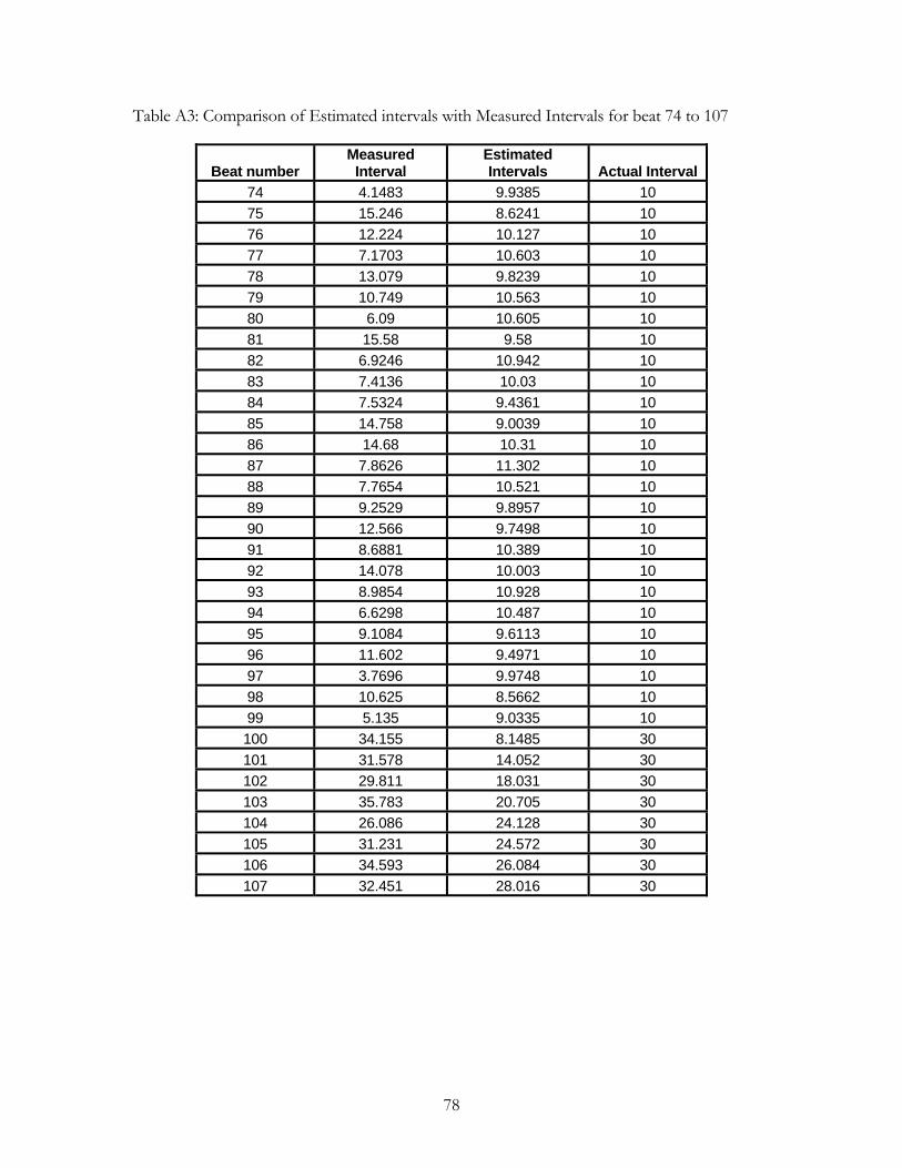
Table A3: Comparison of Estimated intervals with Measured Intervals for beat 74 to 107
Beat number Measured
Interval Estimated Intervals Actual Interval
74 4.1483 9.9385 10 75 15.246 8.6241 10 76 12.224 10.127 10 77 7.1703 10.603 10 78 13.079 9.8239 10 79 10.749 10.563 10 80 6.09 10.605 10 81 15.58 9.58 10 82 6.9246 10.942 10 83 7.4136 10.03 10 84 7.5324 9.4361 10 85 14.758 9.0039 10 86 14.68 10.31 10 87 7.8626 11.302 10 88 7.7654 10.521 10 89 9.2529 9.8957 10 90 12.566 9.7498 10 91 8.6881 10.389 10 92 14.078 10.003 10 93 8.9854 10.928 10 94 6.6298 10.487 10 95 9.1084 9.6113 10 96 11.602 9.4971 10 97 3.7696 9.9748 10 98 10.625 8.5662 10 99 5.135 9.0335 10 100 34.155 8.1485 30 101 31.578 14.052 30 102 29.811 18.031 30 103 35.783 20.705 30 104 26.086 24.128 30 105 31.231 24.572 30 106 34.593 26.084 30 107 32.451 28.016 30
78

Table A4: Comparison of Estimated intervals with Measured Intervals for beat 108 to 140
Beat number Measured
Interval Estimated Intervals Actual Interval
108 30.532 29.022 30 109 34.714 29.365 30 110 33.518 30.579 30 111 32.173 31.246 30 112 28.524 31.457 30 113 32.131 30.791 30 114 31.875 31.095 30 115 27.604 31.272 30 116 33.616 30.439 30 117 30.558 31.16 30 118 27.104 31.024 30 119 36.253 30.134 30 120 30.308 31.523 30 121 25.371 31.247 30 122 28.455 29.913 30 123 26.33 29.582 30 124 26.178 28.844 30 125 30.185 28.239 30 126 25.981 28.68 30 127 31.597 28.068 30 128 30.973 28.869 30 129 29.89 29.347 30 130 29.246 29.47 30 131 27.767 29.419 30 132 31.819 29.044 30 133 37.25 29.674 30 134 5.594 31.394 10 135 7.6804 25.537 10 136 5.4982 21.483 10 137 12.819 17.855 10 138 12.612 16.712 10 139 9.777 15.781 10 140 11.695 14.418 10
79

Table A5: Comparison of Estimated intervals with Measured Intervals for beat 141 to 171
Beat number Measured
Interval Estimated Intervals Actual Interval
141 8.5963 13.8 10 142 9.7002 12.619 10 143 7.9933 11.956 10 144 7.7162 11.056 10 145 13.469 10.298 10 146 6.9273 11.018 10 147 10.69 10.089 10 148 9.1015 10.226 10 149 6.163 9.9706 10 150 10.349 9.1062 10 151 11.703 9.3884 10 152 9.9774 9.9139 10 153 16.471 9.9283 10 154 11.625 11.414 10 155 12.491 11.462 10 156 9.067 11.695 10 157 7.5236 11.099 10 158 11.014 10.287 10 159 6.5627 10.452 10 160 14.165 9.5692 10 161 9.1841 10.613 10 162 15.945 10.288 10 163 7.6881 11.572 10 164 10.073 10.691 10 165 16.835 10.551 10 166 4.2327 11.977 10 167 5.2648 10.219 10 168 12.547 9.0945 10 169 8.2877 9.8782 10 170 13.615 9.5171 10 171 13.401 10.447 10
80

Table A6: Comparison of Estimated intervals with Measured Intervals for beat 172 to 204
Beat number Measured
Interval Estimated Intervals Actual Interval
172 10.399 11.118 10 173 8.4269 10.955 10 174 10.251 10.381 10 175 8.8628 10.352 10 176 7.1772 10.014 10 177 7.4068 9.3697 10 178 14.627 8.9241 10 179 10.644 10.219 10 180 14.013 10.315 10 181 14.797 11.155 10 182 9.2207 11.982 10 183 11.629 11.355 10 184 7.8006 11.417 10 185 6.8926 10.596 10 186 9.1369 9.7554 10 187 10.414 9.615 10 188 5.0793 9.7965 10 189 9.2386 8.7257 10 190 7.9213 8.8421 10 191 7.3737 8.6331 10 192 8.8217 8.3472 10 193 12.784 8.4549 10 194 2.5555 9.4376 10 195 11.532 7.8753 10 196 9.3205 8.7055 10 197 10.193 8.8451 10 198 7.0283 9.1511 10 199 7.3618 8.6692 10 200 5.903 8.3724 10 201 8.4746 7.8118 10 202 14.823 7.9623 10 203 10.781 9.5198 10 204 7.4183 9.806 10
81

Table A7: Comparison of Estimated intervals with Measured Intervals for beat 205 to 230
Beat number Measured
Interval Estimated Intervals Actual Interval
205 17.877 9.264 10 206 7.0688 11.219 10 207 11.893 10.277 10 208 9.471 10.644 10 209 13.056 10.378 10 210 8.5538 10.986 10 211 6.696 10.434 10 212 13.873 9.5851 10 213 7.8787 10.558 10 214 9.4321 9.9501 10 215 11.403 9.8325 10 216 11.112 10.189 10 217 4.6715 10.399 10 218 12.475 9.0985 10 219 11.741 9.8651 10 220 13.401 10.291 10 221 13.784 10.997 10 222 11.434 11.63 10 223 10.439 11.585 10 224 15.882 11.325 10 225 4.8837 12.359 10 226 3.179 10.662 10 227 14.773 8.9636 10 228 11.989 10.282 10 229 14.58 10.67 10 230 7.4579 11.558 10
82

APPENDIX B
MATLAB SOURCE CODE
83
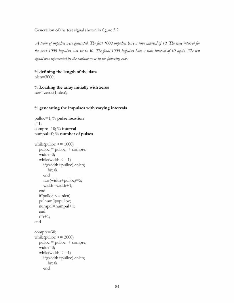
Generation of the test signal shown in figure 3.2.
A train of impulses were generated. The first 1000 impulses have a time interval of 10. The time interval for
the next 1000 impulses was set to 30. The final 1000 impulses have a time interval of 10 again. The test
signal was represented by the variable raw in the following code.
% defining the length of the data nlen=3000; % Loading the array initially with zeros raw=zeros(1,nlen); % generating the impulses with varying intervals pulloc=1; % pulse location i=1; compre=10; % interval numpul=0; % number of pulses while(pulloc <= 1000) pulloc = pulloc + compre; width=0; while(width <= 1) if((width+pulloc)>nlen) break end raw(width+pulloc)=5; width=width+1; end if(pulloc <= nlen) pulnum(i)=pulloc; numpul=numpul+1; end i=i+1; end compre=30; while(pulloc <= 2000) pulloc = pulloc + compre; width=0; while(width <= 1) if((width+pulloc)>nlen) break end
84

raw(width+pulloc)=5; width=width+1; end if(pulloc <= nlen) pulnum(i)=pulloc; numpul=numpul+1; end i=i+1; end compre=10; while(pulloc <= nlen) pulloc = pulloc + compre; width=0; while(width <= 1) if((width+pulloc)>nlen) break end raw(width+pulloc)=5; width=width+1; end if(pulloc <= nlen) pulnum(i)=pulloc; numpul=numpul+1; end i=i+1; end
Calculation of the RR interval and implementation of the KALMAN filter on the test signal
The time interval between the impulses in the test signal are computed and stored in the variable orginterval.
A copy of the interval data is taken into the variable interval so that the interval can be corrupted with the
measurement noise for the noise performance study of the filter. The variable intervalesti gives the estimated
values from the filter. Q and V represent the process and measurement noise covariance.
% calculating the intervals for index=1:numpul-1 orginterval(index)=pulnum(index+1)-pulnum(index); end plen=length(orginterval); % length of the interval array error=randn(1,plen);
85

% process and measurement noise covariance Q=0.5; V=0.1; error=error*sqrt(V); % measurement noise that corrupts the RR interval for index=1:numpul-1 % interval(index)=orginterval(index)+error(index); interval(index)=orginterval(index); end kallen=index; % length of the KALMAN filter % estimating the measured intervals using KALMAN filter % preallocate memory for all arrays intervalesti=zeros(1,kallen); xaposteriori=zeros(1,kallen); residual=zeros(1,kallen); papriori=ones(1,kallen); paposteriori=ones(1,kallen); k=zeros(1,kallen); % define the system a=1; % State transition matrix h=1; % Measurement matrix % initial guesses for state and aposteriri covariance xaposteriori_0=2; paposteriori_0=1; % predictor equations xapriori(1)=a*xaposteriori_0; intervalesti(1)=h*xapriori(1); residual(1)=interval(1)-intervalesti(1); papriori(1)=a*a*paposteriori_0+Q; % corrector equations k(1)=h*papriori(1)/(h*h*papriori(1)+V); paposteriori(1)=papriori(1)*(1-h*k(1)); xaposteriori(1)=xapriori(1)+k(1)*residual(1); % calculating the rest of the values
86

for j=2:kallen % predictor equations xapriori(j)=a*xaposteriori(j-1); intervalesti(j)=h*xapriori(j); residual(j)=interval(j)-intervalesti(j); papriori(j)=a*a*paposteriori(j-1)+Q; % corrector equations k(j)=h*papriori(j)/(h*h*papriori(j)+V); paposteriori(j)=papriori(j)*(1-h*k(j)); xaposteriori(j)=xapriori(j)+k(j)*residual(j); end end
Implementation of the KALMAN filter on ECG recordings from MIT/BIH database.
The first section of the code reads the ECG recordings from the MIT/BIH database which are stored in a
special file format (212 format). The second section of the code processes the ECG data obtained from the
database and performs the QRS detection. The output of the QRS detection is a train of impulses, with
impulses located at the occurrence of a QRS complex in the ECG. Finally, the RR intervals are computed from
this data and passed on to the KALMAN filter algorithm for estimation.
% Reading the ECG files from the database % Specify Data PATH='C:\ thesis\ecg\MIT-BIHArrhythmia Database'; % path, where data are saved HEADERFILE= '102.hea'; % header-file in text format ATRFILE= '102.atr'; % attributes-file in binary format DATAFILE='102.dat'; % data-file SAMPLES2READ=15000; % number of samples to be read % load header data fprintf(1,'\\n$> WORKING ON %s ...\n', HEADERFILE); signalh= fullfile(PATH, HEADERFILE); fid1=fopen(signalh,'r'); z=fgetl(fid1); A= sscanf(z, '%*s %d %d %d',[1,3]); nosig= A(1); % number of signals
87
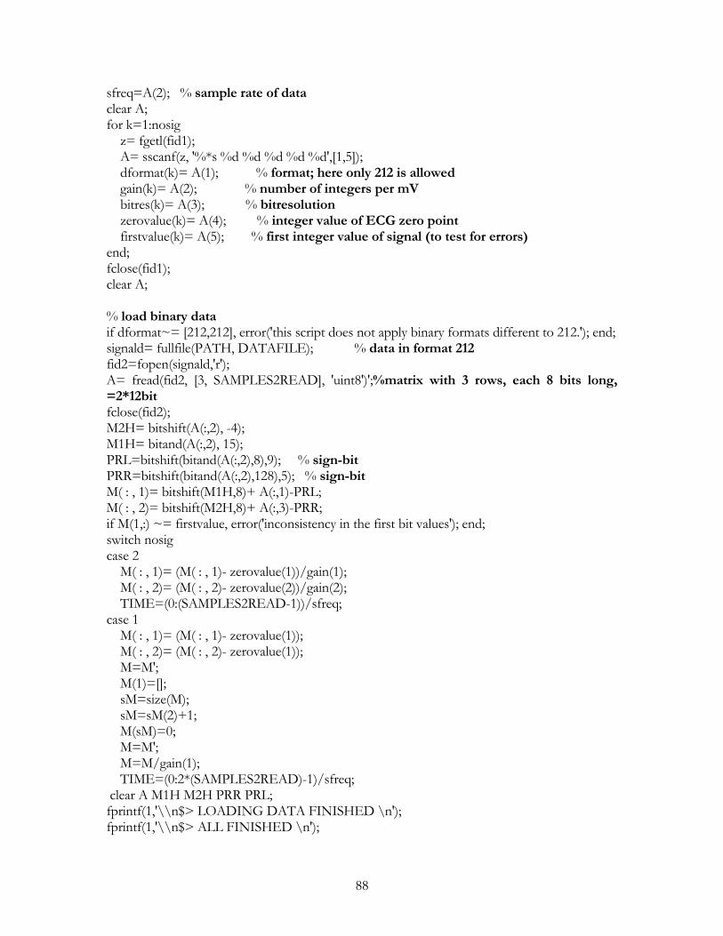
sfreq=A(2); % sample rate of data clear A; for k=1:nosig z= fgetl(fid1); A= sscanf(z, '%*s %d %d %d %d %d',[1,5]); dformat(k)= A(1); % format; here only 212 is allowed gain(k)= A(2); % number of integers per mV bitres(k)= A(3); % bitresolution zerovalue(k)= A(4); % integer value of ECG zero point firstvalue(k)= A(5); % first integer value of signal (to test for errors) end; fclose(fid1); clear A; % load binary data if dformat~= [212,212], error('this script does not apply binary formats different to 212.'); end; signald= fullfile(PATH, DATAFILE); % data in format 212 fid2=fopen(signald,'r'); A= fread(fid2, [3, SAMPLES2READ], 'uint8')';%matrix with 3 rows, each 8 bits long, =2*12bit fclose(fid2); M2H= bitshift(A(:,2), -4); M1H= bitand(A(:,2), 15); PRL=bitshift(bitand(A(:,2),8),9); % sign-bit PRR=bitshift(bitand(A(:,2),128),5); % sign-bit M( : , 1)= bitshift(M1H,8)+ A(:,1)-PRL; M( : , 2)= bitshift(M2H,8)+ A(:,3)-PRR; if M(1,:) ~= firstvalue, error('inconsistency in the first bit values'); end; switch nosig case 2 M( : , 1)= (M( : , 1)- zerovalue(1))/gain(1); M( : , 2)= (M( : , 2)- zerovalue(2))/gain(2); TIME=(0:(SAMPLES2READ-1))/sfreq; case 1 M( : , 1)= (M( : , 1)- zerovalue(1)); M( : , 2)= (M( : , 2)- zerovalue(1)); M=M'; M(1)=[]; sM=size(M); sM=sM(2)+1; M(sM)=0; M=M'; M=M/gain(1); TIME=(0:2*(SAMPLES2READ)-1)/sfreq; clear A M1H M2H PRR PRL; fprintf(1,'\\n$> LOADING DATA FINISHED \n'); fprintf(1,'\\n$> ALL FINISHED \n');
88

% QRS DETECTION x1=M(:,1); time=TIME; % initialization area ylp=zeros(1,length(x1)); yhp=zeros(1,length(x1)); yavg=zeros(1,length(x1)); ymov=zeros(1,length(x1)); yder=zeros(1,length(x1)); yout=zeros(1,length(x1)); thresholdf1=zeros(1,length(x1)); thresholdf2=zeros(1,length(x1)); thresholdi1=zeros(1,length(x1)); thresholdi2=zeros(1,length(x1)); spkf=zeros(1,500); npkf=zeros(1,500); spki=zeros(1,500); npki=zeros(1,500); period=max(time)/length(time); t=0; N=37; % this is the width of the integration window latency=30; % this is the delay for which a second signal can't be used as a QRS times=0; qmax=zeros(2,length(x1)); wmax=zeros(2,length(x1)); out=zeros(1,length(x1)); fout=zeros(1,length(x1)+50); iout=zeros(1,length(x1)); a=0; b=0; delay=0; k=2; %filter peak variable d=2; %integrator peak variable set=1; %these next 2 flags allow for finding the peaks let=1; spkf(1)=0; npkf(1)=0; spki(1)=0; npki(1)=0; RRsum=0; n=0; count=0; t=0; e=0;
89

RRavg1=0; RRavg2=0; wcount=0; countp=0; intmax=0; filtmax=0; %this is the main loop of the program. the input is incrementally stepped %through the filter, derivative, integration, etc. the delays in %processing are taken into account using the if statements to make sure the %data is used at the correct time. for i=13:length(x1), %ylp is the output of the low pass filter ylp(i)=(x1(i)-2*x1(i-6)+x1(i-12)+2*ylp(i-1)-ylp(i-2)); if i>32 %yhp is the output of the bandpass filter yhp(i)=(yhp(i-1)-ylp(i)/32+ylp(i-16)-ylp(i-17)+ylp(i-32)/32); end if i>35 %increments the search window filtmax=filtmax+1; if filtmax==50 qmax(1,k)=yhp(i); qmax(2,k)=i; for p=0:50 if yhp(i-p)>qmax(1,k) %the max and location are stored in this variable. this %max could be either signal or noise. qmax(1,k)=yhp(i-p); qmax(2,k)=i-p; end end filtmax=0; peakf=qmax; spkf(1)=qmax(1,2); %set=0; if n<3 %if n is small the peaks are based on the previous peaks if qmax(1,k)>qmax(1,k-1) spkf(k)=.125*peakf(1,k)+.875*spkf(k-1); npkf(k)=npkf(k-1); else npkf(k)=.125*peakf(1,k)+.875*npkf(k-1); spkf(k)=spkf(k-1); end else %once several peaks are determined, the sinal peak is
90

%determined if it is within a certain range of a known peak if (.85*qpk(n-1)<qmax(1,k))&(qmax(1,k)<1.15*qpk(n-1)) spkf(k)=.125*peakf(1,k)+.875*spkf(k-1); npkf(k)=npkf(k-1); else npkf(k)=.125*peakf(1,k)+.875*npkf(k-1); spkf(k)=spkf(k-1); end end %determines the threshold value of this range thresholdf1(k)=npkf(k)+.25*(spkf(k)-npkf(k)); thresholdf2(k)=.5*thresholdf1(k); %determines if the signal of the specified range is greater or %less than the threshold of that range and rewrites the output %relative to the main i variable for p=0:49 if yhp(i-p)>thresholdf1(k)%&(wmax(2,d-1)+latency)<i fout(i-p)=1; else fout(i-p)=0; end end %increment the peak variable k=k+1; end if i==500+35 %this corresponds to 2seconds(the largest time needed for 1 beat [a t]=max(qmax(1,:)); %finds maximum point after several max locations n=1; for m=1:length(qmax) %qpk are the peaks that are within an allowable maximum, %whereas qmax is all peaks which will include noise peaks if (.85*a<qmax(1,m))&(qmax(1,m)<1.15*a) qpk(1,n)=qmax(1,m); qpk(2,n)=qmax(2,m); %once the first RR is found, the other variable based %on this can be started if n>1 RR(n)=qpk(2,n)-qpk(2,n-1); RRsum=RRsum+RR(n); RRavg2=RRavg1; RRlow=.92*RRavg2; RRhigh=1.16*RRavg2; RRmiss=1.67*RRavg2; end n=n+1; end end
91

end %once i is large enough, a the program can continulally search for %peaks and continually update the RR's if i>=500+35 %determines a range of acceptable peaks of qrs if (.85*a<qmax(1,k))&(qmax(1,k)<1.15*a) qpk(1,n)=qmax(1,k); qpk(2,n)=qmax(2,k); RR(n)=qpk(2,n)-qpk(2,n-1); %this determines the averages if there are 8 or fewer RR %intervals if n<9 RRsum=RRsum+RR(n); RRavg1=RRsum/(n-1); RRavg2=RRavg1; end RRavg1=((RRavg1*.875)+.125*RR(n)); %this if statement determines RRbar and keeps track of how %often RRbar is equal to RR. if (RR(n)<RRhigh) & (RR(n)>RRlow) RRbar(n)=RR(n); RRavg2=.875*RRavg2+.125*RRbar(n); count=count+1; if count==8 RRavg2=RRavg1; end else count=0; end RRlow=.92*RRavg2; RRhigh=1.16*RRavg2; RRmiss=1.67*RRavg2; n=n+1; end %once several RR's are established, we can start looking for %missed peaks if n>3 if (i-qpk(2,n-1))>RRmiss thresholdf1(k-1)=thresholdf2(k-1); [peak t2]=max(peakf(1,qpk(2,n-2)+latency:i)); qpk(1,n-1)=peak; qpk(2,n-1)=t2+qpk(2,n-2); spkf(k-1)=0.25*peakf(1,k-1)+0.75*spkf(k-2); RR(n-1)=qpk(2,n-1)-qpk(2,n-2); if (RR(n-1)<RRhigh) & (RR(n-1)>RRlow) RRbar(n-1)=RR(n-1); RRavg2=.875*RRavg2+.125*RRbar(n-1); count=count+1;
92
if count==8 RRavg2=RRavg1; end else count=0; end end end end end %this is the start of the integration process with the derivative and %the square outputs if i>36 yder(i)=0.125*(2*yhp(i)+yhp(i-1)-yhp(i-3)-2*yhp(i-4)); ysq(i)=yder(i)*yder(i); end %this is the start of the moving average integrator where is the size %of the window and yavg is the output that will be sent to the %threshold detector if i>72 for j=0:N-1 ymov(i)=ymov(i)+ysq(i-j); end yavg(i)=ymov(i)/(N); %this section determines a maximum for a certain window(50samples) intmax=intmax+1; if intmax==50 wmax(1,d)=yavg(i); wmax(2,d)=i; for p=0:50 if yavg(i-p)>wmax(1,d) %the max and location are stored in this variable. this %max could be either signal or noise. wmax(1,d)=yavg(i-p); wmax(2,d)=i-p; end end intmax=0; %this initializer the first peak as a signal peak spki(1)=wmax(1,2); %let=0; peaki=wmax; thresholdi1(d)=npki(d-1)+.25*(spki(d-1)-npki(d-1)); thresholdi2(d)=.5*thresholdi1(d); %average width of the integration window out from the threshold %filter is equal to this delay
93
delay=40; %runs the average signal through the threshold at the same %window interval that the threshold was determined for p=0:49 if yavg(i-p)>thresholdi1(d) iout(i-p)=1; else iout(i-p)=0; end end %this for loop determines the output based on the delay. it is %done here because we just calculated the iout(the most delayed %signal). for p=0:49 %we want to delay the fout signal by half the delay of the %integration output fdout(i-p)=fout(i-p-ceil(delay/2)); out(i-p)=fdout(i-p)*iout(i-p); end %this determines whether the peak is a signal or noise peak if wmax(1,d)>wmax(1,d-1) spki(d)=.125*peaki(1,d)+.875*spki(d-1); npki(d)=npki(d-1); else npki(d)=.125*peaki(1,d)+.875*npki(d-1); spki(d)=spki(d-1); end %the d variable is only incremented when there is a new peak d=d+1; %peak incrementer end end %once d and n are large enough. a missed peak in the integration area %can be determined if d>3 & n>3 if wmax(2,d-2)+RRmiss<i thresholdi1(d-1)=thresholdi2(d-1); [peak t3]=max(peaki(1,wmax(2,d-2)+latency:i)); wmax(1,d-1)=peak; wmax(2,d-1)=t3+wmax(2,d-2); spki(d-1)=0.25*peaki(1,d-1)+0.75*spki(d-2); end end end
94

% KALMAN algorithm implementation % calculating the RR Intervals from the QRS detector Output nlen=length(x1); numpul=0; index=4; while(index <= nlen) if (out(index-2)==0 && out(index)==1 && out(index-1)==0) numpul=numpul+1; pullocation(numpul)=index; index=index+160; else index=index+1; end end plen=length(pullocation); for index=1:plen-1; orginterval(index)=time(pullocation(index+1))-time(pullocation(index)); interval(index)=time(pullocation(index+1))-time(pullocation(index)); end kallen=plen-1; % estimating the measured intervals using kalman filter % preallocate memory for all arrays intervalesti=zeros(1,kallen); xaposteriori=zeros(1,kallen); residual=zeros(1,kallen); papriori=ones(1,kallen); paposteriori=ones(1,kallen); k=zeros(1,kallen); % define the system a=1; % State transition matrix h=1; % Measurement matrix Q=1; % Process noise covariance V=0.02; % Measurement noise covariance % initial guesses for state and aposteriri covariance xaposteriori_0=0.6; paposteriori_0=1;
95
% predictor equations xapriori(1)=a*xaposteriori_0; intervalesti(1)=h*xapriori(1); residual(1)=interval(1)-intervalesti(1); papriori(1)=a*a*paposteriori_0+Q; % corrector equations k(1)=h*papriori(1)/(h*h*papriori(1)+V); paposteriori(1)=papriori(1)*(1-h*k(1)); xaposteriori(1)=xapriori(1)+k(1)*residual(1); % calculating the rest of the values for j=2:kallen % predictor equations xapriori(j)=a*xaposteriori(j-1); intervalesti(j)=h*xapriori(j); residual(j)=interval(j)-intervalesti(j); papriori(j)=a*a*paposteriori(j-1)+Q; % corrector equations k(j)=h*papriori(j)/(h*h*papriori(j)+V); paposteriori(j)=papriori(j)*(1-h*k(j)); xaposteriori(j)=xapriori(j)+k(j)*residual(j); end end
96

LIST OF REFERENCES
1. Klabunde, R.E., www.cvphysiology.com, 2004.
2. Texas Heart Institute, http://www.texasheartinstitute.org/conduct.html
3. Tony Lacey, http://www.cc.gatech.edu/classes/cs7322_98_spring/PS/kf1.pdf
4. http://innovexpo.itee.uq.edu.au/2001/projects/s369535/image1.jpg
5. A comparison of the noise sensitivity of nine QRS detection algorithms. Friesen GM,
Jannett TC, Jadallah MA, Yates SL, Quint SR, Nagle HT
6. A real-time QRS detection algorithm. Pan J, Tompkins W.
7. Real time electrocardiogram QRS detection using combined adaptive threshold Ivaylo
I Christov.
8. ECG beat detection using filter banks. Afonso VX, Tompkins WJ, Nguyen TQ, Luo
S.
9. Least Squares estimation: from Gauss to Kalman. H.W.Sorenson.
10. A new approach to Linear filtering and prediction problems. R.E.Kalman.
11. Estimation of Non-stationary EEG with Kalman Smoother Approach: an Application
to Event-Related Synchronization (ERS). M.P. Tarvainen, J.K. Hiltunen, P.O. Ranta-
aho, and P.A. Karjalainen
12. Round-Trip Time Estimation In Communication Networks Using Adaptive Kalman
Filtering. Krister Jacobsson, Håkan Hjalmarsson, Niels Möller,Karl Henrik Johansson.
13. Real-time Estimation of Human Body Postures using Kalman Filter. Kazuhiko
Takahashi, Tatsumi Sakaguchi, and Jun Ohya
14. DIGITAL FILTERS analysis, design and applications. Andreas Antonio
15. ADAPTIVE SIGNAL PROCESSING. Bernard Widrow, Samuel D.Stearns
97

16. ADAPTIVE FILTERING Algorithms and Practical Implementation. Paulo S. R.
Diniz
17. www.embedded.com/story/OEG20010529S0118. Kalman Filtering. Dan Simon
18. HEART RATE VARIABILITY, Marek Malik, A. John Camm
19. http://butler.cc.tut.fi/~malmivuo/bem/bembook/15/15.htm
20. http://ecg.mit.edu
21. http://physionet.org
98