

Rotational Trading System - Monty Pelerin's World
41
Dynamic Momentum Trading Developed by Monty Pelerin
Transcript of Rotational Trading System - Monty Pelerin's World

P a g e | 2
Summary and Disclaimer
Executive Summary
Successful rotational-based trading depends on timely identification of stock trends. Trends persist beyond what efficient market adherents can explain. Spotting trends early provides opportunity for excess gain.
ETFs (exchange traded funds trade like stocks and mirror market sectors, industries and indices. The diversification and quick entry and exit make them excellent candidates for rotational trading.
The development of a proprietary and dynamic momentum measurement has provided superior backtest results over the last 10 years. The description of this system and its performance are the subject of this paper.
Disclaimer
This presentation is not financial advice. Momentum rankings are presented as a tool which may be useful in your trading. Backtest results may be unique to the time and ETFs used. There is no assurance future rankings will produce comparable results.
Reasonable attempts are made to process momentum rankings in an accurate and timely fashion. Data accuracy and availability depends on a chain of vendors and subsequent processing. No guarantee of rank accuracy is made.
Meaningful financial decisions should be reviewed with a trusted and qualified financial adviser. I am not a financial adviser. I do not make recommendations.
I provide information only and comment on it. How you use this information is up to you.
This is not financial advice. Use the information as you see fit. You do so at your own risk.

P a g e | 3
Chapter One – Introduction
Scope of Project
This paper will cover a lot of ground and include the following topics:
1. Rationale for momentum-based investing. 2. Analyze the process of developing a Dynamic Momentum Trading. 3. Review multiple sets of backtest results. 4. Develop a Simple Switching System (SSS) which can be used to filter Dynamic
Momentum trades. 5. The process to settle on one trading system. 6. Review of the ranking and trading cycles.
What is Momentum Investing?
A general definition of momentum and how it pertains to investing is provided by AQR:
“Momentum is the phenomenon that securities which have performed well relative to peers (winners) on average continue to outperform, and securities that have performed relatively poorly (losers) tend to continue to underperform.”
Efficient Market Hypothesis (EMH) advocates claim there is no mechanical trading strategy that outperforms markets on a consistent basis. Research in this area began almost sixty years ago as a joint project between Merrill Lynch and the University of Chicago. Eugene Fama, considered the strongest advocate of EMH, was awarded a Nobel Prize for his work in this area. (To learn more about efficient markets, try this article.)
The one anomaly that EMH adherents have difficulty explaining is the positive bias of momentum trading:
“Momentum, in my view, is the biggest embarrassment for efficient markets,” Fama said, admitting that he was “hoping it goes away.” [Source]
[On a personal level, I had Dr. Fama as a professor at the University of Chicago (and also played basketball with him in lunch-time pick-up games). He was the second-best professor I had, exceeded only by Milton Friedman. Fama was objective, intellectually honest and provided great clarity in class. While highly competitive on the basketball court, he would not receive a Nobel Prize for his ability in this area, nor would any of the rest of us who partook in these lunchtime games.]
How is Momentum Measured?
There is no official way to define and measure momentum in the investment field. Many technical indicators purport to measure it. Some include momentum in their names.

P a g e | 4
Momentum is a measure of change over time. For investors, to the extent that momentum has predictive value, some measure of price change is generally developed.
Technical analysts will recognize most oscillators (stochastics, MACD, RSI, etc.) as a form of momentum measurement. These measures, used alone, tell whether a security is near the top of its expected (imagined?) range or near the bottom. Those using such tools typically buy near the low point of the oscillator and sell near the high.
Rotational trading needs more than the application of an oscillator. The concept of relative strength is necessary. Strength of different securities must be measured on a comparable basis to determine a ranking of strengths.
A simple (and likely ineffective) rotational trading system could be achieved by comparing the oscillator values of different securities against one another. These values would then be rank ordered from best to worst. The best would be deemed the candidate most likely to succeed in a trade.
Relative ranking is the key to rotational trading.
A Simple Momentum-based System
Approaches to momentum can be simple and be effective. For example, a popular subscription-based website has a model that allows users to create their own momentum-based systems. The approach consists of three variables -- two measures of return and one measure of volatility. Users specify the time periods over which the measures are calculated and then the importance of each via a weighting system.
The system is a black box but here is my impression of what goes on inside the box. Each stock or ETF is has three values for each of the variables. For each variable each security is ranked by the value of its standing from 1 to n (where n is the number of securities). These rank-orders are then weighted by the weights selected to produce a composite total score. This composite score is then rank-ordered. The highest (lowest) ranked assets are then bought (sold).
The system is simple and polished. As a former subscriber, I recommend it for those who want to try momentum trading. The site used to allow limited free testing and perhaps still does.
Dynamic Momentum
A dynamic momentum system differs from a static one. The subscription system just described is static. Regardless of market conditions, the variables do not change and the weights do not either. This measure of momentum, no matter how sophisticated, is static because the parameters in the system never change.
P a g e | 5
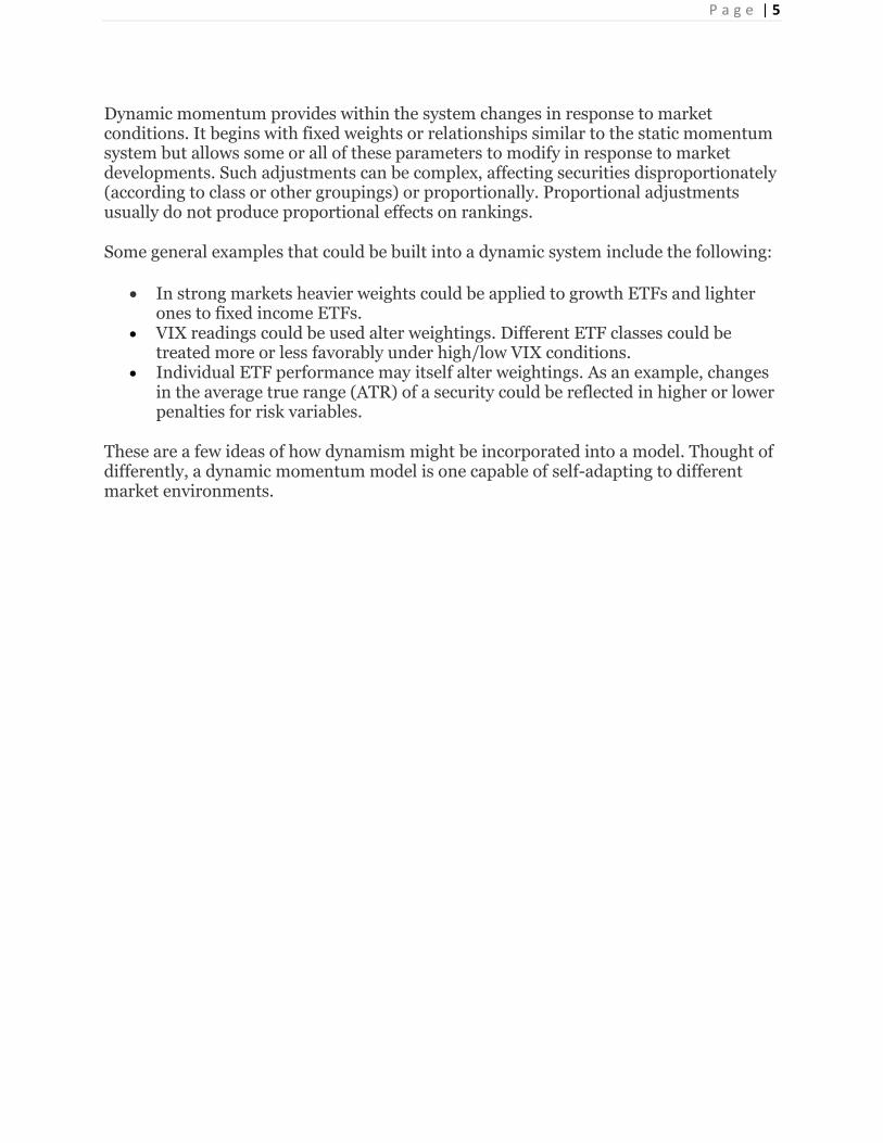
Dynamic momentum provides within the system changes in response to market conditions. It begins with fixed weights or relationships similar to the static momentum system but allows some or all of these parameters to modify in response to market developments. Such adjustments can be complex, affecting securities disproportionately (according to class or other groupings) or proportionally. Proportional adjustments usually do not produce proportional effects on rankings.
Some general examples that could be built into a dynamic system include the following:
In strong markets heavier weights could be applied to growth ETFs and lighter ones to fixed income ETFs.
VIX readings could be used alter weightings. Different ETF classes could be treated more or less favorably under high/low VIX conditions.
Individual ETF performance may itself alter weightings. As an example, changes in the average true range (ATR) of a security could be reflected in higher or lower penalties for risk variables.
These are a few ideas of how dynamism might be incorporated into a model. Thought of differently, a dynamic momentum model is one capable of self-adapting to different market environments.

P a g e | 6
Chapter Two -- The DMS System(s)
This chapter introduces the ETF Dynamic Momentum Trading System. From here forward, DMS (dynamic momentum system) will be used interchangeably to refer to the system.
Uniqueness – Dynamic Adjustments
The ETF Dynamic Momentum Trading System (DMS) differs from other momentum approaches in that it allows variables and weights to self-modify in response to market conditions.
These relationships are built into the model, complex and proprietary. It is the self-modifying adjustments market conditions that account for the superior profit results. Economic judgments and rationalizations of various valuation models guided the
programming of these proprietary relationships.
System Options
Variables were established as user options for testing purposes. These were variables that could not reasonably be determined by a priori or valuation considerations. One could think of these as situational options. That is, the uniqueness of the situation rather than general valuation considerations determine their optimum value.
An example of one such variable would be the optimum number of trades a system should take to maximize its outcomes. If the universe of securities being drawn from is ten, this is likely a low number. If the universe of securities is 1,000 or more, then it is likely that the preferred number of trades is higher.
Where economic theory could not provide guidance, empirical testing was used.
There are only three system variables. Ultimately, these are narrowed down to where followers of the system need make no choices. These were established for development purposes so that empirical testing could establish those situationally correct to the type of trading chosen.
The variables that were tested are the following:
1. Trading Style (3 different styles – Normal, Aggressive and Conservative) 2. Number of Trades (1, 2, 3, or 4 trades per month were tested) 3. Type of Trading (Long Only trades and a combination of Long and Short)
The very first of these, “Trading Style,” was incorporated to allow users to select a trading style consistent with their risk appetite. These choices altered the balance between risk and return among the trading styles.
P a g e | 7
Trading style effects will be apparent in the backtest output. The three styles did not accomplish all that I had hoped, although more work in this area could likely improve them. Additional effort in this area was ignored when it was decided not to issue the model to the public. However, as will be seen in this paper, the ability to generate meaningful rotational rankings is not compromised.
For the impatient, the system that is ultimately decided upon is Normal trading style with one trade per month and long only.
There is value in going through the development process. While some will consider this tedious, it does provide a better understanding of the model development and trading processes.
More importantly, it provides a sense of the robustness of the system. “Robustness” describes the sensitivity of the system to changes in inputs. A system is said to be robust if the success of the system holds over different input choices.
In all, 24 combinations of options were possible and backtests were produced for each combination. The rationale for selecting TN1 (Trading Normal, 1 trade, long only) as the preferred set of options is explained.
DMS Long
This project anticipated long trades only. That objective never changed, although the efficacy of short trading was explored. This section deals with the outcomes from Long Only trades. The next section will look at the effects of short trades.
The permutations and combinations of options for DMS Long Only trades are in the table below. The period is from January 1, 2007 through mid-day December 1, 2016. The style and pos columns on the right side of the table indicate which trading style and the number of positions traded. The definitions of Style and Pos are as follows:
Style: 1 = Normal, 2 = Aggressive and 3 = Conservative.
Pos are the number of trades per month which range from 1 to 4.
Column definitions are:
CAR: compound annual return,
Big Neg Trade and Big Sys Loss are adverse loss conditions. The first represents the worst percentage drop from a single trade. The second represents the largest drawdown (peak equity to trough equity) also referred to as maximum system drawdown or MDD. Both are calculated at month ends.
Car%/BigSys is compound annual return divided by the maximum system drawdown (MDD). The higher this number the better. It measures compound annual return relative to maximum drawdown.
Sharpe Ratio is a common measurement used to evaluate performance.
P a g e | 8
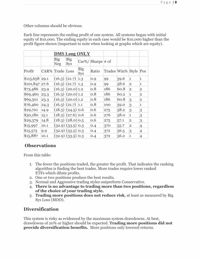
Other columns should be obvious.
Each line represents the ending profit of one system. All systems began with initial equity of $10,000. The ending equity in each case would be $10,000 higher than the profit figure shown (important to note when looking at graphs which are equity).
DMS Long ONLY
Big Neg
Big Sys
Car%/ Sharpe # of
Profit CAR% Trade Loss Big Sys
Ratio Trades Win% Style Pos
$115,658 29.1 (16.3) (21.7) 1.3 0.9 99 59.6 1 1
$101,847 27.6 (16.3) (21.7) 1.3 0.9 99 58.6 2 1
$73,486 23.9 (16.3) (20.0) 1.2 0.8 186 60.8 2 2
$69,460 23.3 (16.3) (20.0) 1.2 0.8 186 60.2 1 2
$69,501 23.3 (16.3) (20.0) 1.2 0.8 186 60.8 3 2
$76,460 24.3 (16.3) (21.7) 1.1 0.8 100 59.0 3 1
$29,701 14.9 (18.3) (24.5) 0.6 0.6 275 58.2 3 3
$30,180 15.1 (18.3) (27.6) 0.6 0.6 276 58.0 1 3
$29,379 14.8 (18.3) (28.0) 0.5 0.6 275 57.1 2 3
$15,997 10.1 (32.9) (33.5) 0.3 0.4 370 55.7 2 4
$15,575 9.9 (32.9) (33.5) 0.3 0.4 372 56.5 3 4
$15,887 10.1 (32.9) (33.5) 0.3 0.4 372 56.2 1 4
Observations
From this table:
1. The fewer the positions traded, the greater the profit. That indicates the ranking algorithm is finding the best trades. More trades require lower ranked ETFs which dilute profits.
2. One or two positions produce the best results. 3. Normal and Aggressive trading styles outperform Conservative. 4. There is no advantage to trading more than two positions, regardless
of the choice of your trading style. 5. Trading more positions does not reduce risk, at least as measured by Big
Sys Loss (MDD).
Diversification
This system is risky as evidenced by the maximum system drawdowns. At best, drawdowns of 20% or higher should be expected. Trading more positions did not provide diversification benefits. More positions only lowered returns.

P a g e | 9
Anyone trading this system should invest the bulk of his/her funds conventionally. That is, asset diversification and the beneficial effects of risk reduction must be achieved via other holdings not highly correlated with these selections.
Stated differently, funds committed to the DMS Long Only strategy should be a small part of an otherwise diversified investment program.
Simple Switching System (SSS) A Simple Switching System (SSS) can be used to mitigate DMS risk. SSS will be discussed in Chapter Eight.
P a g e | 10
Chapter Three -- DMS Long and Short
During the development process, it was decided to test short trades for the purpose of further evaluating the dynamic momentum ranking effectiveness.
Just as highest-ranked securities are more likely to outperform, lowest-ranked securities are expected to underperform. Effective momentum measures identify winners and losers.
Low momentum rankings could be capitalized by selling securities short. Doing so, would produce profits if the securities did indeed drop in value.
Short-Selling Caveat(s)
The ability to test short selling was added to the model for testing purposes. Short-selling is riskier than traditional buys and is not advocated. Higher risk comes from the fact that short-selling can produce losses in excess of what you thought you had invested.
Short-selling is prohibited in IRA accounts. For major ETF categories like indices or bonds, contra or inverse ETFs are available.
For backtesting purposes, actual ETFs are traded as if they could be shorted. In reality, the supply of securities available for short-selling may restrict one from accomplishing short sales even if he/she is trading a regular brokerage account.
[Inverse ETFs may be reviewed in the future. There are no plans to include them into the universe of ranked securities. If there are inverse funds that match up to normal ETFs, these may be highlighted.]
Short-selling is not recommended. Its effects are tested in the next section only as another look at the effectiveness of the momentum ranking system.
New System – DMS Long and Short
The DMS Long and Short system is identical to the DMS Long Only system in terms of user choices. What is different is the effects of short-selling included in the results. The system tested is actually a combined long and short system:
If two ETFs are traded, one is traded long and the other short. Long takes priority, so if you trade only one ETF, it will be a long position. If you trade two it will be one long and one short. Three is two longs and one short and four is two of each.
P a g e | 11
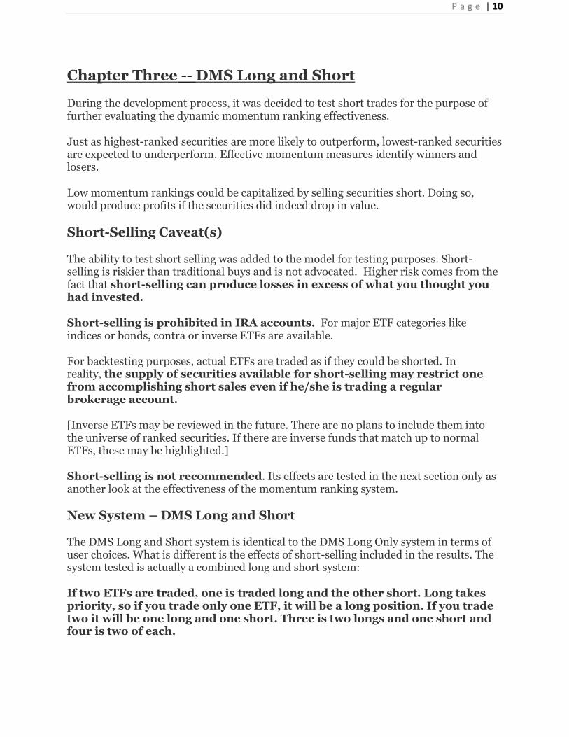
Backtest results for the long and short strategy are shown below. Columns and time periods are the same as in the previous Long Only table.
DMS Long & Short
Big
Neg
Big
Sys Car%/ Sharpe # of
Profit CAR% Trade Loss Big
Sys Ratio Trades Win% Style Pos
$115,658 29.1 (16.3) (21.7) 1.3 0.9 99 59.6 1 1
$101,847 27.6 (16.3) (21.7) 1.3 0.9 99 58.6 2 1
$76,460 24.3 (16.3) (21.7) 1.1 0.8 100 59.0 3 1
$56,309 21.0 (32.8) (15.5) 1.4 0.6 203 55.7 2 2
$60,324 21.8 (32.8) (15.5) 1.4 0.7 203 56.7 3 2
$71,740 23.6 (32.8) (15.5) 1.5 0.7 201 56.7 1 2
$61,126 21.9 (32.8) (12.9) 1.7 0.7 288 58.0 1 3
$63,048 22.2 (32.8) (12.9) 1.7 0.7 289 58.5 3 3
$55,966 21.0 (32.8) (12.9) 1.6 0.7 290 57.9 2 3
$49,848 19.8 (32.8) (11.3) 1.8 0.6 383 56.9 3 4
$47,133 19.2 (32.8) (12.0) 1.6 0.6 383 56.7 2 4
$43,961 18.5 (32.8) (12.0) 1.6 0.6 384 56.5 1 4
Observations
Some observations from this table:
1. Styles with only one trade produce the same results as in the Long Only table because the position is always long.
2. While more trades generally produce lower profits, the drop-off in profit is not nearly as severe as the DMS Long Only system.
3. Diversification benefits, at least in terms of maximum system drawdown, do occur with this system as more trades are taken.
4. Two positions (one long and one short) produce comparable profit to the DMS Long Only 2 trades. About 10% more trades are taken but lower risk as reflected in the maximum drawdowns is achieved.
5. Beyond two trades, this system is superior to the DMS Long Only system in both profit and risk.
The DMS Long and Short Momentum System was an academic exercise. It validates the efficacy of the momentum ranking measure for both long and short use. It also shows such a mixed system reduces risk. It will not be pursued as a regular system in this paper.
Low ranked ETFs could be provided each month for informational purposes.

P a g e | 12
Chapter Four – Benchmarking
A trading system should be evaluated against a benchmark to assess its efficacy. A common benchmark is the S&P 500 index. It is diversified and provides a reasonable example of what a passive investment (“buy and hold”) strategy might achieve.
Buy and Hold
SPY, the ETF representing the S&P 500, will be used as the benchmark.
If the momentum-based systems work, one would expect them to produce higher returns than a buy and hold strategy. Similarly, because they invest in few assets, it is reasonable that they be of higher risk than SPY.
The results are surprising:
Buying SPY January 2007 with $10,000 and holding it until Dec. 1, 2016 produced a profit of only $5,491. This profit was dwarfed by all of the 24 backtests reported.
The differences are startling! The best of the momentum-based strategies produced returns twenty times better than buy and hold. The worst were triple the SPY outcome.
Using maximum system drawdown as a proxy for risk, SPY shocked again. The buy and hold strategy produced a maximum system drawdown of 55%, despite having almost 500 more stocks than the momentum systems. The worst DMS system had a drawdown of 21.7%.
The buy and hold strategy, in short, produced terrible returns in comparison. It also had a much higher maximum drawdown.
Is momentum trading a silver bullet? Perhaps, but these are backtest results. There is no guarantee that such out-performance will continue.
Markets change and so do the efficacies of systems. The period from 2001 through 2016 had some rough road. So, too will the future. Will the system hold up?
Another Comparison
To say one system is better than another based on a few statistics is dangerous. Hidden in summary statistics could be very good or very poor periods. Disaggregation of returns into smaller time periods can provide a better look.
One way to do this is to look at annual returns. Some obvious questions should be addressed:
Is a positive (or negative) ten-year result due to one or two great (or poor) years?
P a g e | 13
Does a system show consistency over time?
Is the underperformance of SPY solely the result of the market collapse that began in late 2007?
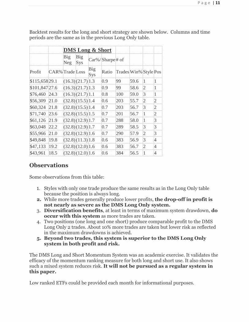
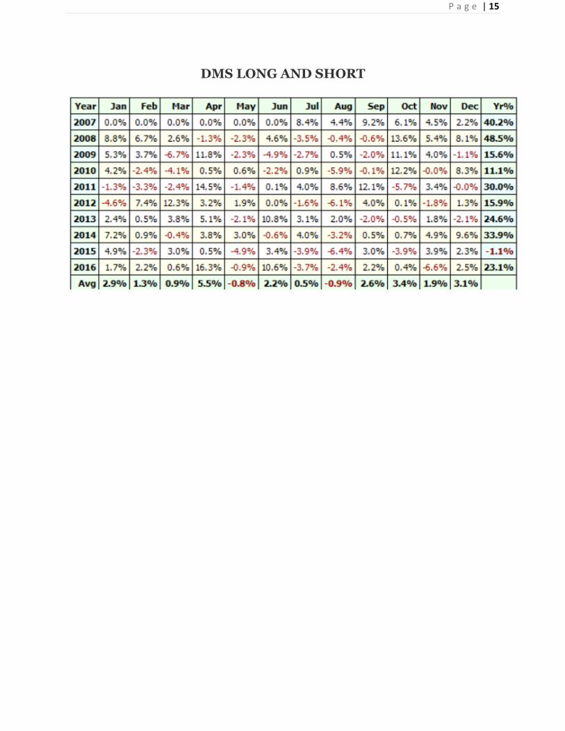
The DMS Long Only system and the DMS Long and Short System will be compared to SPY on an annual basis. While DMS Long and Short is not intended to be a working system, it provides another test of whether the dynamic momentum ranking works.
For the DMS Long and DMS Long and Short, the normal trading style with two positions (TN2) will be used (two trades are needed to get one short trade).
The table below compares annual percentage returns of the DMS Long & Short system (on the left) and the DMS Long Only system (on the right) with SPY (BH Yr%). The greenish yellow boxes to the left of each column show where the momentum systems outperformed SPY in a year by 5% points or more. Likewise, the Red arrows show where SPY outperformed the momentum system by more than 5% points.
DMS LONG & SHORT |DMS Long ONLY
Observations
The following observations are pertinent:
In both instances, SPY only outperformed its momentum comparison two years out of ten.

P a g e | 14
Momentum systems outperformed in both cases. In one instance they did so in seven years; in the other, five years.
The market decline in 2007 and 2008 allowed the Long & Short strategy to greatly outperform both DMS Long and SPY but hardly can be cited as the reason for the differences.
Based on this time frame and this momentum algorithm, both systems are judged consistently better than a buy and hold strategy using the S&P500 as a benchmark. Yearly results support the 10-year conclusions.
Further Disaggregation
Results can be further disaggregated to diagnose the relative performances of each of the systems versus the benchmark or against each other. For example, each of the systems can be shown in terms of monthly returns.
We have likely gone too far for most readers. But, to end this section, the two trading systems are presented as monthly percentage returns. Perhaps viewing the month-to-month volatility will be of use to readers.
DMS LONG ONLY
P a g e | 15
DMS LONG AND SHORT
P a g e | 16
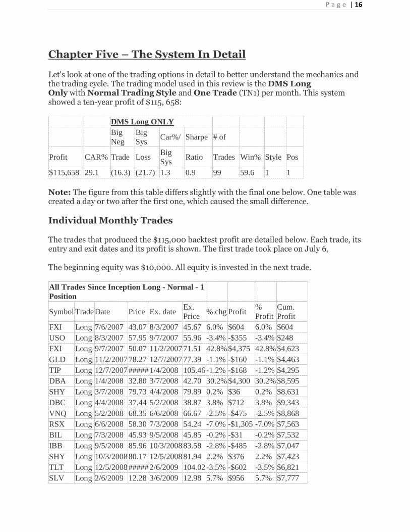
Chapter Five – The System In Detail
Let's look at one of the trading options in detail to better understand the mechanics and the trading cycle. The trading model used in this review is the DMS Long Only with Normal Trading Style and One Trade (TN1) per month. This system showed a ten-year profit of $115, 658:
DMS Long ONLY
Big
Neg
Big
Sys Car%/ Sharpe # of
Profit CAR% Trade Loss Big
Sys Ratio Trades Win% Style Pos
$115,658 29.1 (16.3) (21.7) 1.3 0.9 99 59.6 1 1
Note: The figure from this table differs slightly with the final one below. One table was created a day or two after the first one, which caused the small difference.
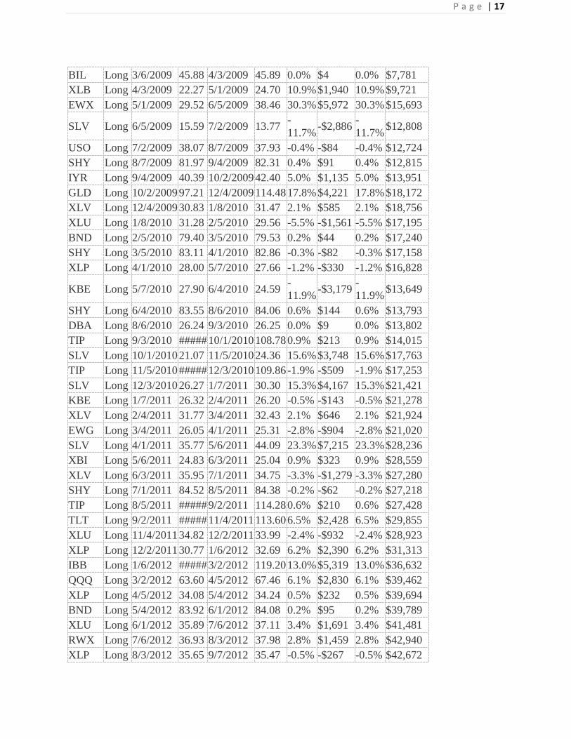
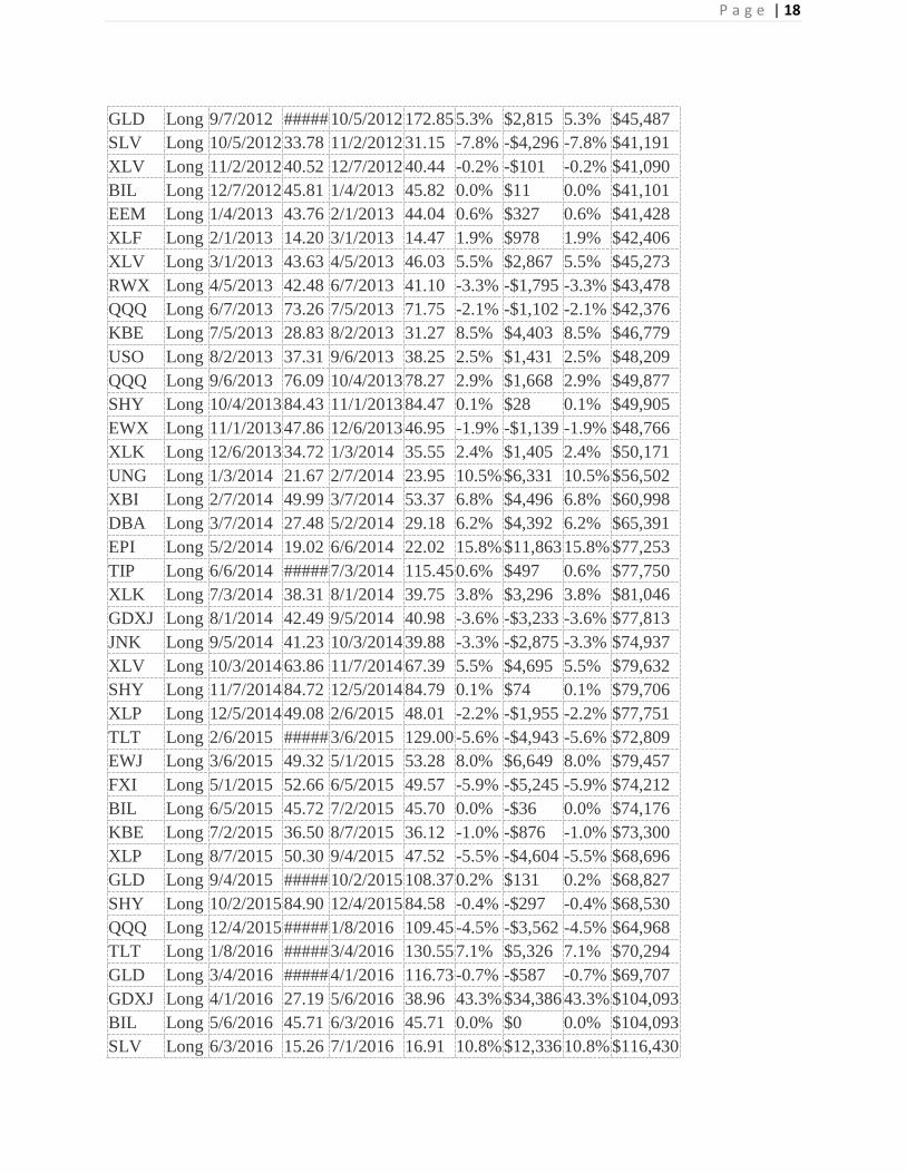
Individual Monthly Trades
The trades that produced the $115,000 backtest profit are detailed below. Each trade, its entry and exit dates and its profit is shown. The first trade took place on July 6,
The beginning equity was $10,000. All equity is invested in the next trade.
All Trades Since Inception Long - Normal - 1
Position
Symbol Trade Date Price Ex. date Ex.
Price % chg Profit
%
Profit
Cum.
Profit
FXI Long 7/6/2007 43.07 8/3/2007 45.67 6.0% $604 6.0% $604
USO Long 8/3/2007 57.95 9/7/2007 55.96 -3.4% -$355 -3.4% $248
FXI Long 9/7/2007 50.07 11/2/2007 71.51 42.8% $4,375 42.8% $4,623
GLD Long 11/2/2007 78.27 12/7/2007 77.39 -1.1% -$160 -1.1% $4,463
TIP Long 12/7/2007 ##### 1/4/2008 105.46 -1.2% -$168 -1.2% $4,295
DBA Long 1/4/2008 32.80 3/7/2008 42.70 30.2% $4,300 30.2% $8,595
SHY Long 3/7/2008 79.73 4/4/2008 79.89 0.2% $36 0.2% $8,631
DBC Long 4/4/2008 37.44 5/2/2008 38.87 3.8% $712 3.8% $9,343
VNQ Long 5/2/2008 68.35 6/6/2008 66.67 -2.5% -$475 -2.5% $8,868
RSX Long 6/6/2008 58.30 7/3/2008 54.24 -7.0% -$1,305 -7.0% $7,563
BIL Long 7/3/2008 45.93 9/5/2008 45.85 -0.2% -$31 -0.2% $7,532
IBB Long 9/5/2008 85.96 10/3/2008 83.58 -2.8% -$485 -2.8% $7,047
SHY Long 10/3/2008 80.17 12/5/2008 81.94 2.2% $376 2.2% $7,423
TLT Long 12/5/2008 ##### 2/6/2009 104.02 -3.5% -$602 -3.5% $6,821
SLV Long 2/6/2009 12.28 3/6/2009 12.98 5.7% $956 5.7% $7,777
P a g e | 17
BIL Long 3/6/2009 45.88 4/3/2009 45.89 0.0% $4 0.0% $7,781
XLB Long 4/3/2009 22.27 5/1/2009 24.70 10.9% $1,940 10.9% $9,721
EWX Long 5/1/2009 29.52 6/5/2009 38.46 30.3% $5,972 30.3% $15,693
SLV Long 6/5/2009 15.59 7/2/2009 13.77 -
11.7% -$2,886
-
11.7% $12,808
USO Long 7/2/2009 38.07 8/7/2009 37.93 -0.4% -$84 -0.4% $12,724
SHY Long 8/7/2009 81.97 9/4/2009 82.31 0.4% $91 0.4% $12,815
IYR Long 9/4/2009 40.39 10/2/2009 42.40 5.0% $1,135 5.0% $13,951
GLD Long 10/2/2009 97.21 12/4/2009 114.48 17.8% $4,221 17.8% $18,172
XLV Long 12/4/2009 30.83 1/8/2010 31.47 2.1% $585 2.1% $18,756
XLU Long 1/8/2010 31.28 2/5/2010 29.56 -5.5% -$1,561 -5.5% $17,195
BND Long 2/5/2010 79.40 3/5/2010 79.53 0.2% $44 0.2% $17,240
SHY Long 3/5/2010 83.11 4/1/2010 82.86 -0.3% -$82 -0.3% $17,158
XLP Long 4/1/2010 28.00 5/7/2010 27.66 -1.2% -$330 -1.2% $16,828
KBE Long 5/7/2010 27.90 6/4/2010 24.59 -
11.9% -$3,179
-
11.9% $13,649
SHY Long 6/4/2010 83.55 8/6/2010 84.06 0.6% $144 0.6% $13,793
DBA Long 8/6/2010 26.24 9/3/2010 26.25 0.0% $9 0.0% $13,802
TIP Long 9/3/2010 ##### 10/1/2010 108.78 0.9% $213 0.9% $14,015
SLV Long 10/1/2010 21.07 11/5/2010 24.36 15.6% $3,748 15.6% $17,763
TIP Long 11/5/2010 ##### 12/3/2010 109.86 -1.9% -$509 -1.9% $17,253
SLV Long 12/3/2010 26.27 1/7/2011 30.30 15.3% $4,167 15.3% $21,421
KBE Long 1/7/2011 26.32 2/4/2011 26.20 -0.5% -$143 -0.5% $21,278
XLV Long 2/4/2011 31.77 3/4/2011 32.43 2.1% $646 2.1% $21,924
EWG Long 3/4/2011 26.05 4/1/2011 25.31 -2.8% -$904 -2.8% $21,020
SLV Long 4/1/2011 35.77 5/6/2011 44.09 23.3% $7,215 23.3% $28,236
XBI Long 5/6/2011 24.83 6/3/2011 25.04 0.9% $323 0.9% $28,559
XLV Long 6/3/2011 35.95 7/1/2011 34.75 -3.3% -$1,279 -3.3% $27,280
SHY Long 7/1/2011 84.52 8/5/2011 84.38 -0.2% -$62 -0.2% $27,218
TIP Long 8/5/2011 ##### 9/2/2011 114.28 0.6% $210 0.6% $27,428
TLT Long 9/2/2011 ##### 11/4/2011 113.60 6.5% $2,428 6.5% $29,855
XLU Long 11/4/2011 34.82 12/2/2011 33.99 -2.4% -$932 -2.4% $28,923
XLP Long 12/2/2011 30.77 1/6/2012 32.69 6.2% $2,390 6.2% $31,313
IBB Long 1/6/2012 ##### 3/2/2012 119.20 13.0% $5,319 13.0% $36,632
QQQ Long 3/2/2012 63.60 4/5/2012 67.46 6.1% $2,830 6.1% $39,462
XLP Long 4/5/2012 34.08 5/4/2012 34.24 0.5% $232 0.5% $39,694
BND Long 5/4/2012 83.92 6/1/2012 84.08 0.2% $95 0.2% $39,789
XLU Long 6/1/2012 35.89 7/6/2012 37.11 3.4% $1,691 3.4% $41,481
RWX Long 7/6/2012 36.93 8/3/2012 37.98 2.8% $1,459 2.8% $42,940
XLP Long 8/3/2012 35.65 9/7/2012 35.47 -0.5% -$267 -0.5% $42,672
P a g e | 18
GLD Long 9/7/2012 ##### 10/5/2012 172.85 5.3% $2,815 5.3% $45,487
SLV Long 10/5/2012 33.78 11/2/2012 31.15 -7.8% -$4,296 -7.8% $41,191
XLV Long 11/2/2012 40.52 12/7/2012 40.44 -0.2% -$101 -0.2% $41,090
BIL Long 12/7/2012 45.81 1/4/2013 45.82 0.0% $11 0.0% $41,101
EEM Long 1/4/2013 43.76 2/1/2013 44.04 0.6% $327 0.6% $41,428
XLF Long 2/1/2013 14.20 3/1/2013 14.47 1.9% $978 1.9% $42,406
XLV Long 3/1/2013 43.63 4/5/2013 46.03 5.5% $2,867 5.5% $45,273
RWX Long 4/5/2013 42.48 6/7/2013 41.10 -3.3% -$1,795 -3.3% $43,478
QQQ Long 6/7/2013 73.26 7/5/2013 71.75 -2.1% -$1,102 -2.1% $42,376
KBE Long 7/5/2013 28.83 8/2/2013 31.27 8.5% $4,403 8.5% $46,779
USO Long 8/2/2013 37.31 9/6/2013 38.25 2.5% $1,431 2.5% $48,209
QQQ Long 9/6/2013 76.09 10/4/2013 78.27 2.9% $1,668 2.9% $49,877
SHY Long 10/4/2013 84.43 11/1/2013 84.47 0.1% $28 0.1% $49,905
EWX Long 11/1/2013 47.86 12/6/2013 46.95 -1.9% -$1,139 -1.9% $48,766
XLK Long 12/6/2013 34.72 1/3/2014 35.55 2.4% $1,405 2.4% $50,171
UNG Long 1/3/2014 21.67 2/7/2014 23.95 10.5% $6,331 10.5% $56,502
XBI Long 2/7/2014 49.99 3/7/2014 53.37 6.8% $4,496 6.8% $60,998
DBA Long 3/7/2014 27.48 5/2/2014 29.18 6.2% $4,392 6.2% $65,391
EPI Long 5/2/2014 19.02 6/6/2014 22.02 15.8% $11,863 15.8% $77,253
TIP Long 6/6/2014 ##### 7/3/2014 115.45 0.6% $497 0.6% $77,750
XLK Long 7/3/2014 38.31 8/1/2014 39.75 3.8% $3,296 3.8% $81,046
GDXJ Long 8/1/2014 42.49 9/5/2014 40.98 -3.6% -$3,233 -3.6% $77,813
JNK Long 9/5/2014 41.23 10/3/2014 39.88 -3.3% -$2,875 -3.3% $74,937
XLV Long 10/3/2014 63.86 11/7/2014 67.39 5.5% $4,695 5.5% $79,632
SHY Long 11/7/2014 84.72 12/5/2014 84.79 0.1% $74 0.1% $79,706
XLP Long 12/5/2014 49.08 2/6/2015 48.01 -2.2% -$1,955 -2.2% $77,751
TLT Long 2/6/2015 ##### 3/6/2015 129.00 -5.6% -$4,943 -5.6% $72,809
EWJ Long 3/6/2015 49.32 5/1/2015 53.28 8.0% $6,649 8.0% $79,457
FXI Long 5/1/2015 52.66 6/5/2015 49.57 -5.9% -$5,245 -5.9% $74,212
BIL Long 6/5/2015 45.72 7/2/2015 45.70 0.0% -$36 0.0% $74,176
KBE Long 7/2/2015 36.50 8/7/2015 36.12 -1.0% -$876 -1.0% $73,300
XLP Long 8/7/2015 50.30 9/4/2015 47.52 -5.5% -$4,604 -5.5% $68,696
GLD Long 9/4/2015 ##### 10/2/2015 108.37 0.2% $131 0.2% $68,827
SHY Long 10/2/2015 84.90 12/4/2015 84.58 -0.4% -$297 -0.4% $68,530
QQQ Long 12/4/2015 ##### 1/8/2016 109.45 -4.5% -$3,562 -4.5% $64,968
TLT Long 1/8/2016 ##### 3/4/2016 130.55 7.1% $5,326 7.1% $70,294
GLD Long 3/4/2016 ##### 4/1/2016 116.73 -0.7% -$587 -0.7% $69,707
GDXJ Long 4/1/2016 27.19 5/6/2016 38.96 43.3% $34,386 43.3% $104,093
BIL Long 5/6/2016 45.71 6/3/2016 45.71 0.0% $0 0.0% $104,093
SLV Long 6/3/2016 15.26 7/1/2016 16.91 10.8% $12,336 10.8% $116,430
P a g e | 19
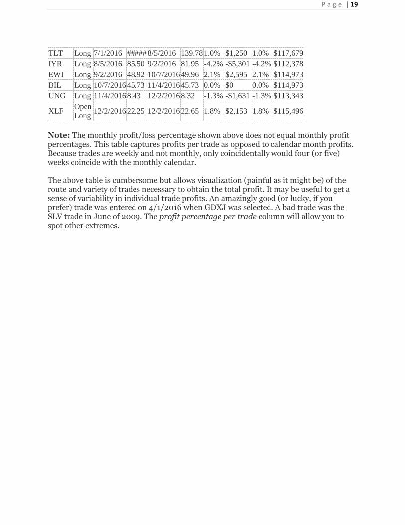
TLT Long 7/1/2016 ##### 8/5/2016 139.78 1.0% $1,250 1.0% $117,679
IYR Long 8/5/2016 85.50 9/2/2016 81.95 -4.2% -$5,301 -4.2% $112,378
EWJ Long 9/2/2016 48.92 10/7/2016 49.96 2.1% $2,595 2.1% $114,973
BIL Long 10/7/2016 45.73 11/4/2016 45.73 0.0% $0 0.0% $114,973
UNG Long 11/4/2016 8.43 12/2/2016 8.32 -1.3% -$1,631 -1.3% $113,343
XLF Open
Long 12/2/2016 22.25 12/2/2016 22.65 1.8% $2,153 1.8% $115,496
Note: The monthly profit/loss percentage shown above does not equal monthly profit percentages. This table captures profits per trade as opposed to calendar month profits. Because trades are weekly and not monthly, only coincidentally would four (or five) weeks coincide with the monthly calendar.
The above table is cumbersome but allows visualization (painful as it might be) of the route and variety of trades necessary to obtain the total profit. It may be useful to get a sense of variability in individual trade profits. An amazingly good (or lucky, if you prefer) trade was entered on 4/1/2016 when GDXJ was selected. A bad trade was the SLV trade in June of 2009. The profit percentage per trade column will allow you to spot other extremes.

P a g e | 20
Chapter Six -- Trade Days and Momentum Rankings
Trades are signaled by two factors: trade-days and momentum rankings.
A trade-day occurs once per month, always the last Friday of the month. Momentum rankings can be calculated any time. (For purposes of backtesting, only the rankings on the last Friday of each month were used for trades. Momentum rankings on other days should have the same meaning as on trade days, although only trade days were backtested.)
Trades are opened/closed at the open price on the Monday following a trade day. The table below shows rankings for a recent set of five trade days. Rankings shown include more ETFs than would be traded, showing the five highest and five lowest momentum ranks.
SOME RECENT RANKINGS
Ticker Date/Time Name Rank
XLF 11/25/2016 SPDRs Select Sector Financial ETF 1
KBE 11/25/2016 SPDR KBW Bank ETF 2
IWM 11/25/2016 iShares Russell 2000 Index Fund ETF 3
DIA 11/25/2016 SPDR Dow Jones Industrial Average ETF 4
RSX 11/25/2016 Market Vectors Russia ETF 5
EWX 11/25/2016 SPDR S&P Emerging Markets Small Cap 41
EEM 11/25/2016 iShares MSCI Emerging Markets Index
Fund ETF 42
TLT 11/25/2016 iShares Barclays 20+ Year Treasury Bond
Fund 43
BND 11/25/2016 Vanguard Total Bond Market ETF 44
EPI 11/25/2016 WisdomTree India Earnings Fund ETF 45
UNG 10/28/2016 US Nat Gas FD ETF 1
TIP 10/28/2016 iShares Barclays TIPS Bond Fund 2
DBC 10/28/2016 PowerShares DB Commodity Index
Tracking ETF 3
XLE 10/28/2016 SPDRs Select Sector Energy ETF 4
USO 10/28/2016 United States Oil Fund LP 5
GDX 10/28/2016 Market Vectors Gold Miners ETF 41
IBB 10/28/2016 iShares Nasdaq Biotechnology Index
Fund ETF 42
XBI 10/28/2016 SPDR S&P Biotech ETF 43
GDXJ 10/28/2016 Market Vectors Junior Gold Miners ETF 44

P a g e | 21
ITB 10/28/2016 iShares Dow Jones US Home
Construction Index Fund ETF 45
BIL 9/30/2016 SPDR Lehman 1-3 Month T-Bill ETF 1
XLU 9/30/2016 SPDRs Select Sector Utilities ETF 2
SHY 9/30/2016 iShares Barclays 1-3 Year Treasury Bond
Fund 3
UNG 9/30/2016 US Nat Gas FD ETF 4
TIP 9/30/2016 iShares Barclays TIPS Bond Fund 5
XLE 9/30/2016 SPDRs Select Sector Energy ETF 41
VNQ 9/30/2016 Vanguard Reit Etf 42
IYR 9/30/2016 iShares Dow Jones US Real Estate Index
Fund ETF 43
GDX 9/30/2016 Market Vectors Gold Miners ETF 44
XLP 9/30/2016 SPDRs Select Sector Consumer Staples
ETF 45
EWJ 8/26/2016 iShares MSCI Japan Index Fund ETF 1
XLK 8/26/2016 SPDRs Select Sector Technology ETF 2
QQQ 8/26/2016 PowerShares QQQTrust Ser 1 3
EWX 8/26/2016 SPDR S&P Emerging Markets Small Cap 4
EWH 8/26/2016 iShares MSCI Hong Kong Index Fund
ETF 5
DBA 8/26/2016 PowerShares DB Agriculture Fund ETF 41
ITB 8/26/2016 iShares Dow Jones US Home
Construction Index Fund ETF 42
VNQ 8/26/2016 Vanguard Reit Etf 43
IYR 8/26/2016 iShares Dow Jones US Real Estate Index
Fund ETF 44
XLV 8/26/2016 SPDRs Select Sector Health Care ETF 45
IYR 7/29/2016 iShares Dow Jones US Real Estate Index
Fund ETF 1
DIA 7/29/2016 SPDR Dow Jones Industrial Average ETF 2
VNQ 7/29/2016 Vanguard Reit Etf 3
SLV 7/29/2016 iShares Silver Trust ETF 4
BND 7/29/2016 Vanguard Total Bond Market ETF 5
XLE 7/29/2016 SPDRs Select Sector Energy ETF 41
SHY 7/29/2016 iShares Barclays 1-3 Year Treasury Bond
Fund 42
DBC 7/29/2016 PowerShares DB Commodity Index
Tracking ETF 43
USO 7/29/2016 United States Oil Fund LP 44
DBA 7/29/2016 PowerShares DB Agriculture Fund ETF 45

P a g e | 22
The system we assume is TN1 (normal trading style with one trade per month). Only long trades are taken. The highest ranked ETF (the one ranked number 1) is entered. Other ranks are shown for informational purposes only.
Were a user trading twice per month, trades ranked 1 and 2 would be entered.
The worst-ranked ETFs, those ranked 41 - 45, could be used if one were interested in shorting poor performers. Number 45 would be the best candidate for a short-trade according to the rankings.
Avoid this Confusion: All trades occur on Monday morning at the opening. All dates in the above tables are at the close of weekly bars, always Friday.
Ranking dates are the last Friday of the month.
Execution dates are the following Monday.
Confusion sometimes occurs because the system uses weekly data and weekly bars. Dates reported are always the end of the week. All executions occur on the Open of that weekly bar.
To illustrate, XLF was selected based on Friday data as of 11/25. It shows a trade dated 12/2, seeming to leave a gap between the signal to buy and the actual buy. The price at which the trade was entered however was the opening price on Monday November 28 which was 22.25. Utilizing weekly instead of daily bars causes this confusion.
Frequent rankings are useful even if they are not used in monthly trading. Rankings will be provided at the end of each week, regardless of whether it is a trade day or not. How you use this information is up to you.
For backtest purposes, trades occur based on trade day rankings.
P a g e | 23
Chapter Seven – The Time Profile of Trades
This section provides a look at the time profile of profits/losses.
It may be skipped by all but the true masochist class of traders. It may be useful once your understanding of the trading cycle, system mechanics is better understood.
The Normal Trading Style of the Dynamic Trading System (DMS) will be used to illustrate. Ranks are shown for the two highest-ranked long trades on trade days.
What to Look For
The purpose of this chapter is to provide the curious a look at how profits or losses develop over time based on momentum rankings. High-ranked rankings are followed for a week, 4 weeks and 13 weeks.
Some of the questions that might be explored are the following:
Is the first week of a trade predictive of the full trade (or in the table below, the first four weeks)?
If a trade begins badly, should it be terminated?
If a trade does well for 4 weeks, does that suggest anything regarding how it performs over 13 weeks?
Readers are left to explore these questions and discern their own answers if there truly are any.
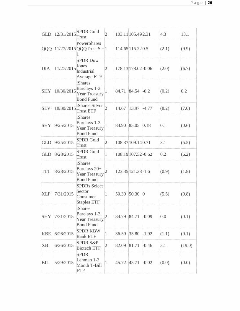
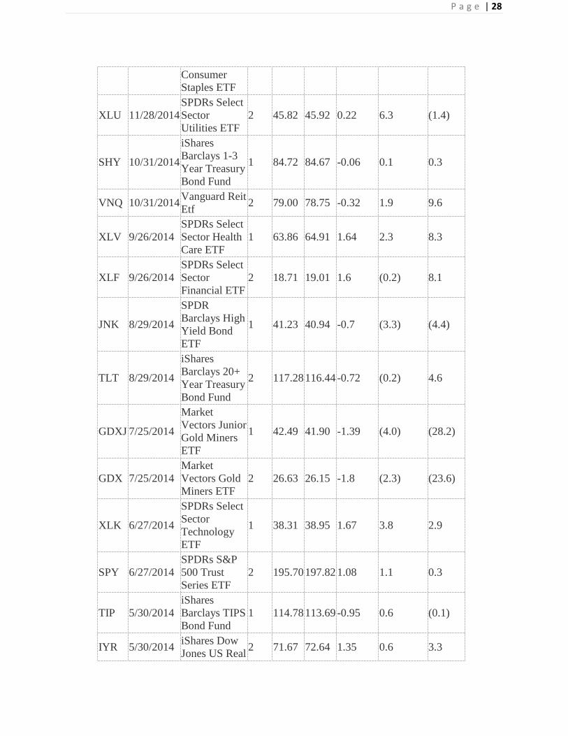
For each ETF, the entry price is shown as is the price one week later (recent entries have no forward-looking data as it was unknown at the time of table creation).
The profit/time profile tracks percentage returns for 1 week, 4 weeks and 13 weeks.
The DMS system is designed to be traded monthly. Thus, the most pertinent column is the 4WkRet%. The 4Wk returns will not agree exactly with prior profit summaries because some of the trades were for five weeks. (The differing starts and ends of months require that some trades are five weeks rather than four.)
The 1 week and 13 week columns are informational only. They allow the reader to judge the pattern of returns over time. Judgments regarding questions like the following may be made:
If a trade starts off badly, how often does it recover?
If a trade is successful for the normal month, is it likely to continue so for the quarter?
How often does the number one ranked trade outperform the second-ranked?

P a g e | 24
These and other judgments may allow readers to determine whether they want to utilize the rankings in a trading program. They may also provide some indication of the risks involved, at least with respect to past performance.
Only a portion of this data is shown:
Normal Trading -- Ranks 1 and 2 Long Only and Trade Days
Ticker Date/Time Name Rank Entry Exit1 WkRet% 4wkRet% 13Ret%
XLF 11/25/2016
SPDRs Select
Sector
Financial ETF
1 22.25 N/A N/A N/A N/A
KBE 11/25/2016 SPDR KBW
Bank ETF 2 40.70 N/A N/A N/A N/A
UNG 10/28/2016 US Nat Gas
FD ETF 1 8.43 7.60 -9.85 (1.3) N/A
TIP 10/28/2016
iShares
Barclays TIPS
Bond Fund
2 115.77 115.70 -0.06 (2.0) N/A
BIL 9/30/2016
SPDR
Lehman 1-3
Month T-Bill
ETF
1 45.73 45.73 0 0.0 0.0
XLU 9/30/2016
SPDRs Select
Sector
Utilities ETF
2 49.01 47.15 -3.8 (0.9) (3.5)
EWJ 8/26/2016
iShares MSCI
Japan Index
Fund ETF
1 48.92 49.80 1.8 2.2 1.8
XLK 8/26/2016
SPDRs Select
Sector
Technology
ETF
2 47.09 47.38 0.62 0.4 1.9
IYR 7/29/2016
iShares Dow
Jones US Real
Estate Index
Fund ETF
1 85.50 83.85 -1.93 (4.2) (11.2)
DIA 7/29/2016
SPDR Dow
Jones
Industrial
Average ETF
2 184.35 185.50 0.62 (0.3) (1.5)
TLT 6/24/2016 iShares
Barclays 20+ 1 138.41 141.85 2.49 0.4 (1.0)

P a g e | 25
Year Treasury
Bond Fund
DBA 6/24/2016
PowerShares
DB
Agriculture
Fund ETF
2 21.73 22.01 1.29 (4.3) (6.2)
SLV 5/27/2016 iShares Silver
Trust ETF 1 15.26 15.63 2.42 10.8 15.9
BIL 5/27/2016
SPDR
Lehman 1-3
Month T-Bill
ETF
2 45.71 45.71 0 (0.0) 0.0
BIL 4/29/2016
SPDR
Lehman 1-3
Month T-Bill
ETF
1 45.71 45.71 0 0.0 0.0
BND 4/29/2016
Vanguard
Total Bond
Market ETF
2 82.78 83.11 0.4 (0.1) 2.0
GDXJ 3/24/2016
Market
Vectors Junior
Gold Miners
ETF
1 27.19 28.16 3.57 24.6 55.1
GDX 3/24/2016
Market
Vectors Gold
Miners ETF
2 19.64 20.05 2.09 15.7 37.5
GLD 2/26/2016 SPDR Gold
Trust 1 117.59 121.18 3.05 (0.7) (1.6)
GDXJ 2/26/2016
Market
Vectors Junior
Gold Miners
ETF
2 25.18 27.55 9.41 8.0 30.6
TLT 1/29/2016
iShares
Barclays 20+
Year Treasury
Bond Fund
1 126.79 129.72 2.31 3.0 1.5
SHY 1/29/2016
iShares
Barclays 1-3
Year Treasury
Bond Fund
2 84.84 85.01 0.2 0.1 0.1
TLT 12/31/2015
iShares
Barclays 20+
Year Treasury
Bond Fund
1 121.89 122.04 0.12 4.0 7.3
P a g e | 26
GLD 12/31/2015 SPDR Gold
Trust 2 103.11 105.49 2.31 4.3 13.1
QQQ 11/27/2015
PowerShares
QQQTrust Ser
1
1 114.65 115.22 0.5 (2.1) (9.9)
DIA 11/27/2015
SPDR Dow
Jones
Industrial
Average ETF
2 178.13 178.02 -0.06 (2.0) (6.7)
SHY 10/30/2015
iShares
Barclays 1-3
Year Treasury
Bond Fund
1 84.71 84.54 -0.2 (0.2) 0.2
SLV 10/30/2015 iShares Silver
Trust ETF 2 14.67 13.97 -4.77 (8.2) (7.0)
SHY 9/25/2015
iShares
Barclays 1-3
Year Treasury
Bond Fund
1 84.90 85.05 0.18 0.1 (0.6)
GLD 9/25/2015 SPDR Gold
Trust 2 108.37 109.14 0.71 3.1 (5.5)
GLD 8/28/2015 SPDR Gold
Trust 1 108.19 107.52 -0.62 0.2 (6.2)
TLT 8/28/2015
iShares
Barclays 20+
Year Treasury
Bond Fund
2 123.35 121.38 -1.6 (0.9) (1.8)
XLP 7/31/2015
SPDRs Select
Sector
Consumer
Staples ETF
1 50.30 50.30 0 (5.5) (0.8)
SHY 7/31/2015
iShares
Barclays 1-3
Year Treasury
Bond Fund
2 84.79 84.71 -0.09 0.0 (0.1)
KBE 6/26/2015 SPDR KBW
Bank ETF 1 36.50 35.80 -1.92 (1.1) (9.1)
XBI 6/26/2015 SPDR S&P
Biotech ETF 2 82.09 81.71 -0.46 3.1 (19.0)
BIL 5/29/2015
SPDR
Lehman 1-3
Month T-Bill
ETF
1 45.72 45.71 -0.02 (0.0) (0.0)

P a g e | 27
EWX 5/29/2015
SPDR S&P
Emerging
Markets Small
Cap
2 47.98 46.36 -3.38 (6.3) (22.3)
FXI 4/24/2015
iShares
FTSE/Xinhua
China 25
Index Fund
ETF
1 52.66 51.61 -1.99 (1.1) (23.9)
EWX 4/24/2015
SPDR S&P
Emerging
Markets Small
Cap
2 47.87 47.89 0.04 0.3 (13.6)
EWJ 3/27/2015
iShares MSCI
Japan Index
Fund ETF
1 51.00 51.12 0.24 4.5 0.9
XLV 3/27/2015
SPDRs Select
Sector Health
Care ETF
2 73.66 71.59 -2.81 1.2 2.3
EWJ 2/27/2015
iShares MSCI
Japan Index
Fund ETF
1 49.32 48.96 -0.73 3.4 6.8
ITB 2/27/2015
iShares Dow
Jones US
Home
Construction
Index Fund
ETF
2 27.62 26.94 -2.46 1.3 (3.1)
TLT 1/30/2015
iShares
Barclays 20+
Year Treasury
Bond Fund
1 136.70 131.97 -3.46 (5.6) (9.1)
BND 1/30/2015
Vanguard
Total Bond
Market ETF
2 83.95 83.27 -0.81 (1.2) (1.6)
XLP 12/26/2014
SPDRs Select
Sector
Consumer
Staples ETF
1 49.40 48.26 -2.31 0.5 (1.6)
XBI 12/26/2014 SPDR S&P
Biotech ETF 2 62.38 62.56 0.29 6.2 19.7
XLP 11/28/2014 SPDRs Select
Sector 1 49.08 48.80 -0.57 0.7 1.8
P a g e | 28
Consumer
Staples ETF
XLU 11/28/2014
SPDRs Select
Sector
Utilities ETF
2 45.82 45.92 0.22 6.3 (1.4)
SHY 10/31/2014
iShares
Barclays 1-3
Year Treasury
Bond Fund
1 84.72 84.67 -0.06 0.1 0.3
VNQ 10/31/2014 Vanguard Reit
Etf 2 79.00 78.75 -0.32 1.9 9.6
XLV 9/26/2014
SPDRs Select
Sector Health
Care ETF
1 63.86 64.91 1.64 2.3 8.3
XLF 9/26/2014
SPDRs Select
Sector
Financial ETF
2 18.71 19.01 1.6 (0.2) 8.1
JNK 8/29/2014
SPDR
Barclays High
Yield Bond
ETF
1 41.23 40.94 -0.7 (3.3) (4.4)
TLT 8/29/2014
iShares
Barclays 20+
Year Treasury
Bond Fund
2 117.28 116.44 -0.72 (0.2) 4.6
GDXJ 7/25/2014
Market
Vectors Junior
Gold Miners
ETF
1 42.49 41.90 -1.39 (4.0) (28.2)
GDX 7/25/2014
Market
Vectors Gold
Miners ETF
2 26.63 26.15 -1.8 (2.3) (23.6)
XLK 6/27/2014
SPDRs Select
Sector
Technology
ETF
1 38.31 38.95 1.67 3.8 2.9
SPY 6/27/2014
SPDRs S&P
500 Trust
Series ETF
2 195.70 197.82 1.08 1.1 0.3
TIP 5/30/2014
iShares
Barclays TIPS
Bond Fund
1 114.78 113.69 -0.95 0.6 (0.1)
IYR 5/30/2014 iShares Dow
Jones US Real 2 71.67 72.64 1.35 0.6 3.3

P a g e | 29
Estate Index
Fund ETF
EPI 4/25/2014
WisdomTree
India Earnings
Fund ETF
1 19.02 19.08 0.32 16.5 17.4
There is a lot of information included above. Use it to visualize the profit/time development. I haven’t analyzed it yet. Don’t be concerned if you skip all these numbers. It isn’t necessary for what lies ahead, but it may be useful in the future.

P a g e | 30
Chapter Eight – The SSS Option
The chapter discusses an option that may be used with the Dynamic Momentum Trading System (DMS).
SSS "System"
The SSS, Simple Switching System, is not a system per se. It is an indicator that may be used in conjunction with DMS. It is an option. .
SSS is a momentum oscillator specifically designed to be used with DMS. It is calculated weekly and registers as "GO" or "STOP." Favorable SSS readings require no change to DMS positions. Unfavorable ones may be used to alter the DMS trade (e.g. lighten up the position or close the position entirely).
SSS modifies the risk of trading DMS. It reduces risk and, in most cases, return. It provides weekly signals which DMS users can use or ignore.
To assess the effects of using SSS, backtest results are presented below. Two sets of results are shown.
Versions of SSS
The first version of SSS, call it SSSHard, assumes exiting a DMS trade and going to cash when the signal reads stop or Red. When the signal returns to go (Green), DMS is re-entered, but only on a trade day. Essentially, exits occur immediately but re-entries occur only once per month (on a trade day signal).
The second version, SSSEasy, is identical to SSSHard with respect to exiting a DMS trade. It differs only in re-entry. Re-entry is assumed whenever the signal turns Green again. It can re-enter on non-trade days.
Because DMS systems are more profitable when not using an SSS filter, getting back in sooner may be a favorable compromise between trading DMS only or DMS with an SSSHard filter. The issue is an empirical one.
Two tables below show each of the SSS backtests...

P a g e | 31
SSSHard Backtest
SSS -- Hard
Big Neg Big
Sys
Car
%
RAR
%
Sharpe
Profit Exp% CAR% RAR% Trade Loss Big
Sys
Big
Sys Ratio Trades Win% pos Style
$48,202 54.6 19.4 35.6 (1198.7) (12.8) 1.5 2.8 1.1 78 60.3 3 1
$46,077 53.7 19.0 35.4 (1154.9) (12.8) 1.5 2.8 1.0 84 59.5 3 3
$39,930 53.5 17.6 32.9 (1168.8) (12.8) 1.4 2.6 1.1 81 61.7 3 2
$41,128 53.9 17.9 33.2 (3362.7) (12.8) 1.2 2.2 1.2 28 60.7 1 1
$54,037 55.0 20.6 37.4 (2201.7) (21.7) 1.0 1.9 1.1 56 67.9 2 2
$53,717 57.3 20.5 35.8 (2201.7) (21.7) 1.0 1.8 1.2 52 71.2 2 3
$47,511 55.6 19.3 34.7 (2201.7) (21.7) 1.0 1.8 1.1 54 68.5 2 1
$32,013 51.9 15.6 30.0 (2763.2) (12.8) 0.9 1.7 1.1 28 57.1 1 2
$28,961 50.4 14.7 29.2 (2562.5) (12.8) 0.9 1.7 1.0 28 57.1 1 3
As in previous articles, Style reflects Normal, Aggressive and Conservative shown as 1, 2, and 3 respectively in the Style column. Pos represents the number of trades.
This table and the one that follows have new columns. These columns measure market exposure. Market exposure (Exp%) is the percentage of time a system is in the market.
DMS systems are virtually 100% invested all the time. SSS filters reduce that. The use of SSS reduces the time DMS is in the market and exposed to market risk.
The new columns in the table above and below are as follows:
In the table above, DMS is in the market just over 50% of the time (Exp% column).
That necessitates an additional column: RAR%. This column adjusts the CAR% (compound annual return) to what its equivalent might be if the funds were invested 100% of the time.
RAR%/Big Sys represents the adjusted CAR in terms of the maximum drawdown (Big Sys Loss).

P a g e | 32
SSSEasy Backtest
SSS -- Easy
Big Neg Big
Sys
Car
% RAR Sharpe
Profit Exp% CAR% RAR% Trade Loss Big
Sys
Big
Sys Ratio Trades Win% pos Style
$69,686 63.5 23.3 36.7 (1700.4) (12.8) 2.1 3.3 1.1 117 65.0 3 1
$68,803 63.3 23.2 36.6 (1681.6) (12.8) 2.1 3.3 1.1 123 64.2 3 3
$66,734 62.9 22.8 36.3 (1698.9) (12.8) 2.1 3.3 1.1 123 65.0 3 2
$49,143 63.9 19.6 30.7 (2235.0) (21.7) 1.1 1.7 0.9 82 52.4 2 2
$47,387 64.3 19.3 30.0 (2235.0) (21.7) 1.1 1.6 0.9 80 55.0 2 1
$47,802 65.1 19.4 29.8 (2235.0) (21.7) 1.1 1.6 0.9 76 54.0 2 3
$44,628 63.7 18.7 29.3 (4020.8) (12.8) 0.9 1.4 0.9 41 53.7 1 1
$39,871 62.0 17.6 28.4 (3670.6) (12.8) 0.9 1.4 0.9 43 53.5 1 3
$39,524 62.0 17.5 28.3 (3645.0) (12.8) 0.9 1.4 0.9 42 54.8 1 2
SSSEasy is less strict (easy) on re-entry. It re-enters whenever the Go signal flashes, not just on a trade day. It has higher market exposure (more than 60%), trades more and produces higher overall profit than SSSHard. It does so with the same maximum system drawdowns.
Note on Number of Trades: The number of trades is understated in both tables. What is counted is the number of trades between the DMS system and cash. If you are trading a DMS system and remain in the system, say for 4 months, and then go to cash, the above table will show two trades -- one to get into DMS and one to go to cash.
The reality is that you are likely adjusting your holding(s) each of the four months in the DMS system. These trades are not counted. In this example, what would show up as two trades could be as many as five.
The understatement of true trades is aggravated more if you are trading a DMS system with more than one trade
SSS vs DMS Backtest Results
Tables for DMS tests from earlier chapters are used with the SSS tables to make these comments on some key metrics:
1. CAR%/Maximum Drawdown -- Slight Advantage SSS Using percentage returns related to maximum system drawdown -- CAR%/Biggest system drawdown (a relative return to risk ranking), the SSS results are more favorable.

P a g e | 33
The five best DMS returns are between 1.2 and 1.3. The five best SSSHard measures are between 1.0 and 1.5. SSSEasy metrics are slightly better: 1.1 - 2.1.
2. RAR%/Maximum Drawdown -- Dominant Advantage SSS
DMS measures are identical to the CAR%/Maximum Drawdowns because these systems are invested 100% of the time. SSSHard range from 1.9 t0 2.8 and SSSEasy from 1.6 to 3.3.
3. Maximum System Drawdowns -- Dominant Advantage SSS
Twelve of the eighteen SSS backtests have maximum drawdowns of 12.8%. The best DMS system has a maximum drawdown of 20%.
4. Sharpe Ratio -- Slight Advantage SSS
SSS outperforms slightly DMS.
5. Total Profits -- Dominant Advantage DMS
Single position DMS systems dwarf the profits of SSS.
6. Profitability -- Slight Advantage DMS
DMS has higher compound annual returns (CAR%) than both SSSHard and SSSEasy.
SSS dominates DMS in terms of RAR%, but that is meaningful only if you have attractive alternative investment options for the cash when out of DMS.
Conclusions
Comparing the DMS only system with the DMS filtered by SSS, the SSS system produces better returns to risk calculations (1 - 4 above). DMS clearly produces more profits (number 5) and dominates in compound annual return.
Once again, the decision as to which is better comes down to risk aversion. Do you prefer a lower, likely safer, return to a higher, riskier, one?
Dynamic momentum trading coupled with the SSS screen enables you to modify the risk-return trade-off of DMS alone.
P a g e | 34
Chapter Nine -- SSS - DMS Integration
This section will show how to integrate the SSS (Simple Switching System) with the DMS (Dynamic Momentum Trading System). It is a review of previous material intended to do the following:
1. Show the simplicity of using weekly rankings. 2. Review (again) the process of Dynamic Momentum Trading (DMS) 3. Integrate the SSS with Dynamic Momentum Trading (DMS).
The Trading Cycle
DMS ranks ETFs utilizing weekly data. The DMS system trades once per month. It offers three trading styles: Normal, Aggressive and Conservative. For DMS, the best backtest results were achieved by trading one ETF using the Normal or Aggressive trading styles. These backtests were presented in earlier chapters.
The key events in a trading cycle are
1. Momentum rankings which are published at the end of each week. 2. The last Friday of each month which is considered a trade day. 3. Monday after a trade day at the Open is when positions are changed.
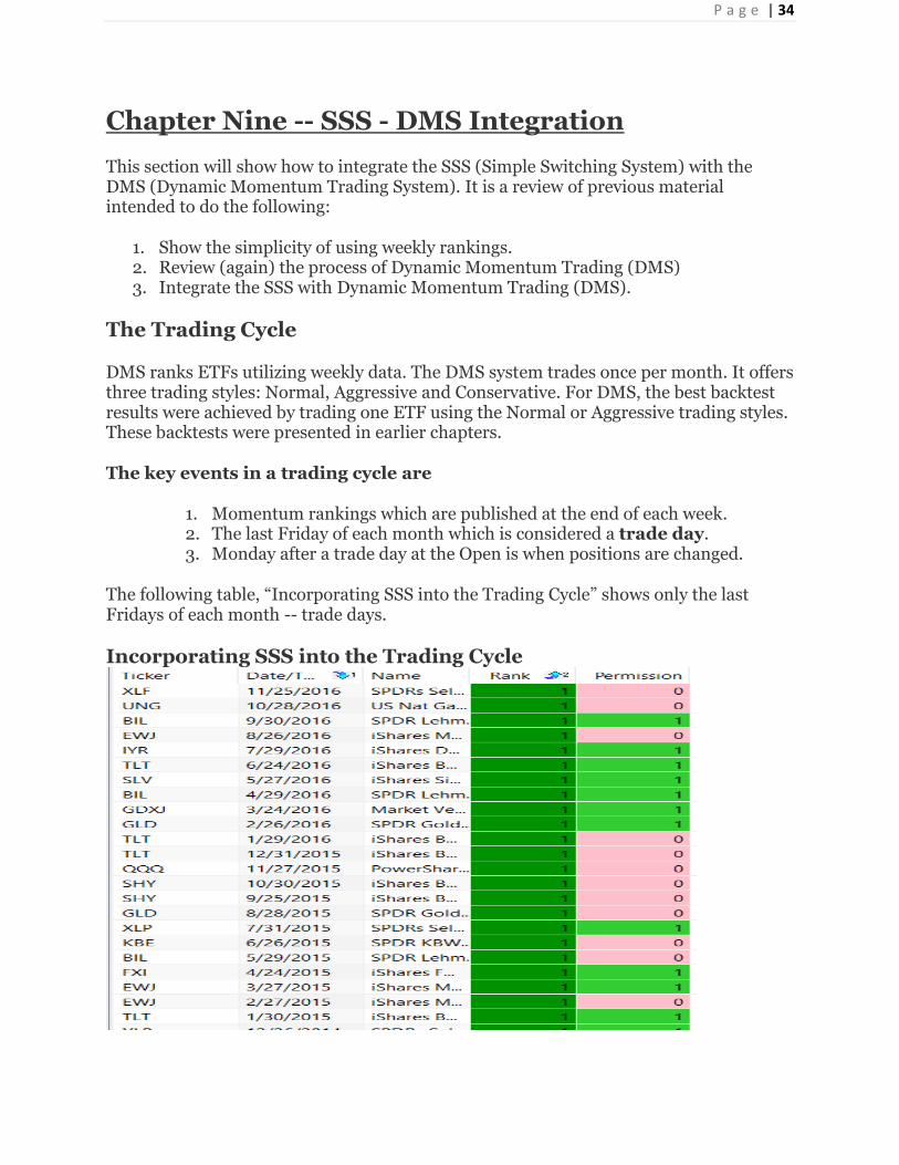
The following table, “Incorporating SSS into the Trading Cycle” shows only the last Fridays of each month -- trade days.
Incorporating SSS into the Trading Cycle

P a g e | 35
The above table shows trade days and the highest ranked ETF on that day (these were trades in the TN1 backtest). The permission column was ignored in the standard DMS trading system(s).
The permission column is color-coded. Lime green is a positive, i.e., go with the trade. Pink is caution or a signal to avoid the trade. If the trade is not taken, the DMS system goes to cash.
If you were utilizing the SSS filter, all trades showing pink in the permission column would not be taken on these trade days.
SSSHard and SSSEasy perform identically on a trade day.
Re-Entry Conditions
Trading SSS Hard only requires the previous table. Trading SSS Easy requires permission signals on all Fridays, not just trade days. This table shows weekly rankings:
P a g e | 36
The ranks for non-trade days are shown in yellow. The yellow weeks matter for SSSEasy trading. To illustrate, one trade will be looked at.
The last trade day (11/25/2016) the highest ranked ETF was XLF. If one were trading DMS only, XLF would have been purchased. If one were trading DMS with an SSS filter, XLF would not have been purchased (pink permission).
The difference between SSS alternatives is what happens regarding re-entry:
SSSHard would remain out of the market until the next trade day.
SSSEasy would enter XLF based on 12/2 (lime permission).
Users may use (or not use) these filters as they choose. The rules for SSSHard and SSSEasy were established primarily to define backtest actions.
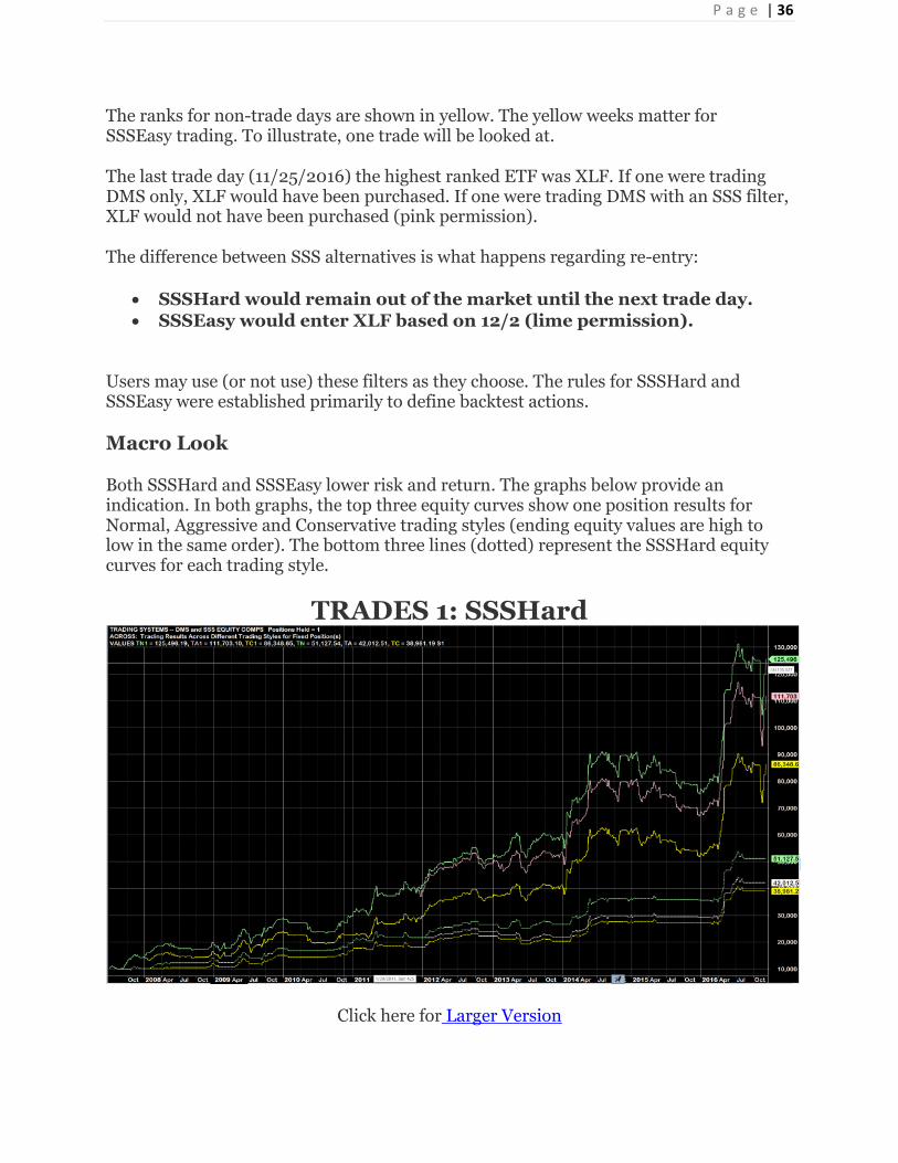
Macro Look
Both SSSHard and SSSEasy lower risk and return. The graphs below provide an indication. In both graphs, the top three equity curves show one position results for Normal, Aggressive and Conservative trading styles (ending equity values are high to low in the same order). The bottom three lines (dotted) represent the SSSHard equity curves for each trading style.
TRADES 1: SSSHard
Click here for Larger Version

P a g e | 37
This chart shows the same information for the DMS trading styles but compares them with SSSEasy results.
TRADES 1: SSSEasy
The ending equity between trading DMS alone and trading DMS with SSS is profound. The best of the SSS curves are the normal trading styles with SSSEasy reporting $54.6K and SSSHard $51.1K. Normal DMS amounted to $125.4K. (It should be remembered that a buy and hold strategy of the S&P 500 produced an ending equity of less than 16K over this same period.)
SSS outcomes improve relative to DMS outcomes as the number of positions increase. No graphs or data are shown because the author, at least at this time, does not feel trading multiple ETFs per month is worthwhile.
A rather comprehensive collection of data has been presented on the ETF momentum rotational trading strategy and its options.
If you are overwhelmed or confused at this point, don't despair. The final chapter clarifies and simplifies all this information.

P a g e | 38
Chapter Ten -- Simplification
The purpose of this section is to narrow down the options in the DMS system without reducing the efficacy of the system.
System Options
The trading model presented had many options, primarily for testing purposes. In systems development, critical variables can be identified more easily than the critical ranges of these variables. Positions to be traded and trading styles were two that fell into this category:
Trading Styles: Three trading styles were built into the momentum algorithm. These were Normal, Aggressive and Conservative.
Number of Positions: The number of ETFs that could be traded ranged from 1 to 3.
The empirics provided by extensive backtesting allows reasonable answers regarding what values should be used to create one trading system.
Selecting a Trading Style
Three trading styles were tested. Differences among these styles were not significant in terms of risk-return considerations. Backtesting results for trading one ETF for each style are presented in the table below.
One Trade Per Month
P a g e | 39
The backtests began January 1, 2007 and ran through December 31, 2016. Each style started with initial equity of $10,000. By the end of 2016 TN1 (light green representing Trading Style Normal and 1 trade per month) had an equity of $133,824. TA1 (pink) and TC1 (yellow) representing Aggressive and Conservative trading styles achieved $119,116 and 106,160, respectively.
The graph above is logarithmic which makes it easier to visualize correlation among the equity curves. Each moves up/down at the same time and roughly the same amounts, evidencing high correlation between them. Put differently, each has similar risk(s). TN1 returned more than TA1 or TC1. Based on similar risk, TN dominates the other two trading styles.
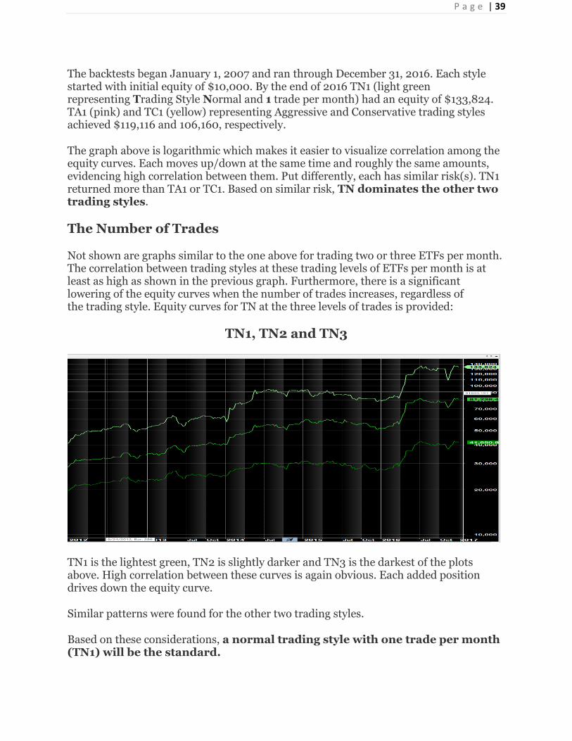
The Number of Trades
Not shown are graphs similar to the one above for trading two or three ETFs per month. The correlation between trading styles at these trading levels of ETFs per month is at least as high as shown in the previous graph. Furthermore, there is a significant lowering of the equity curves when the number of trades increases, regardless of the trading style. Equity curves for TN at the three levels of trades is provided:
TN1, TN2 and TN3
TN1 is the lightest green, TN2 is slightly darker and TN3 is the darkest of the plots above. High correlation between these curves is again obvious. Each added position drives down the equity curve.
Similar patterns were found for the other two trading styles.
Based on these considerations, a normal trading style with one trade per month (TN1) will be the standard.

P a g e | 40
Trading With a Screen (SSS)
The Simple Switching System (SSS) was discussed as a modifier to the DMS system.
SSS can reduce the risks associated with the DMS system. Whether it is for you is a decision that can only be made by you. We all have different risk tolerance. We all have different personal and financial situations.
SSS signals will be provided. Some will use them religiously, some on an intuitive basis and some not at all.
End of the Beginning
Hopefully this presentation has provided educational value regarding system construction, backtesting and the concept of momentum investing. I plan to continue research in the area of dynamic momentum trading, primarily exploring other stock/ETF populations on which to test the model.
Good luck and good trading.
Monty Pelerin
Email: [email protected]
Website: www.economicnoise.com