F

eder

al R

eser

ve B

ank

of C

hica

go

Robustness and Macroeconomic Policy

Gadi Barlevy

WP 2010-04

Robustness and Macroeconomic Policy∗

Gadi Barlevy

Economic Research

Federal Reserve Bank of Chicago

230 South LaSalle

Chicago, IL 60604

e-mail: gbarlevy@frbchi.org

June 29, 2010

Abstract

This paper considers the design of macroeconomic policies in the face of uncertainty. In recent years,

several economists have advocated that when policymakers are uncertain about the environment they

face and find it difficult to assign precise probabilities to the alternative scenarios that may characterize

this environment, they should design policies to be robust in the sense that they minimize the worst-

case loss these policies could ever impose. I review and evaluate the objections cited by critics of this

approach. I further argue that, contrary to what some have inferred, concern about worst-case scenarios

does not always lead to policies that respond more aggressively to incoming news than the optimal

policy would respond absent any uncertainty.

Key Words: Robust Control, Uncertainty, Ambiguity, Attenuation Principle

∗Posted with permission from the Annual Review of Economics, Volume 3 (c) 2011 by Annual Reviews,

http://www.annualreviews.org. I would like to thank Charles Evans for encouraging me to work in this area and Marco

Bassetto, Lars Hansen, Spencer Krane, Charles Manski, Kiminori Matsuyama, Thomas Sargent, and Noah Williams for help-

ful discussions on these issues.

1 Introduction

A recurring theme in the literature on macroeconomic policy concerns the role of uncertainty. In practice,

policymakers are often called to make decisions with only limited knowledge of the environment in which

they operate, in part because they lack all of the relevant data when they are called to act and in part

because they cannot be sure that the models they use to guide their policies are good descriptions of the

environment they face. These limitations raise a question that economists have long grappled with: How

should policymakers proceed when they are uncertain about the environment they operate in?

One seminal contribution in this area comes from Brainard (1967), who considered the case where a

policymaker does not know some of the parameters that are relevant for choosing an appropriate policy

but still knows the probability distribution according to which they are determined. Since the policymaker

knows how the relevant parameters are distributed, he can compute the expected losses that result from

different policies. Brainard solved for the policy that yields the lowest expected loss, and showed that when

the policymaker is uncertain about the effect of his actions, the appropriate response to uncertainty is to

moderate or attenuate the extent to which he should react to the news he does receive. This result has

garnered considerable attention from both researchers and policymakers.1

However, over time economists have grown increasingly critical of the approach inherent in Brainard’s

model to dealing with uncertainty. In particular, they have criticized the notion that policymakers know the

distribution of variables about which they are uncertain. For example, if policymakers do not understand

the environment they face well enough to quite know how to model it, it seems implausible that they can

assign exact probabilities as to what is the right model. Critics who have pushed this line of argument have

instead suggested modelling policymakers as entertaining a class of models that can potentially describe

the data, which is usually constructed as a set of perturbations around some benchmark model, and then

letting policymakers choose policies that are “robust” in the sense that they perform well against all models

in this class. That is, a robust policy is one whose worst performance across all models that policymakers

contemplate exceeds the worst performance of all other policies.

The recommendation that macroeconomic policies be designed to be robust to a class of models remains

controversial. In this paper, I review the debate over the appropriateness of robustness as a criterion for

choosing policy, relying on simple illustrative examples that avoid some of the complicated technicalities

that abound in this literature. I also address a question that preoccupied early work on robustness and

macroeconomic policy, namely, whether robust policies contradict the attenuation result in the original

Brainard model. Although early applications of robustness tended to find that policymakers should respond

1See, for example, the discussion of Brainard’s result in Blinder (1998), pp. 9-13.

1

more aggressively to the news they do receive than they would otherwise, I argue that aggressiveness is not

an inherent feature of robustness but is specific to the models these papers explored. In fact, robustness can

in some environments lead to the same attenuation that Brainard obtained, and for quite similar reasons.

This offers a useful reminder: Results concerning robustness that arise in particular environment will not

always themselves be robust to changes in the underlying environment.

Given space limitations, I restrict my attention to these issues and ignore other applications of robustness

in macroeconomics. For example, there is an extensive literature that studies what happens when private

agents — as opposed to policymakers — choose strategies designed to be robust against a host of models,

and examines whether such behavior can help resolve macroeconomic problems such as the equity premium

puzzle and other puzzles that revolve around attitude toward risk. Readers interested in such questions

should consult Hansen and Sargent (2008) and the references therein. Another line of research considers what

policymakers should do when they know private agents employ robust decisionmaking, but policymakers

are themselves confident about the underlying model of the economy. Examples of such analyses include

Caballero and Krishnamurthy (2008) and Karantounias, Hansen, and Sargent (2009). I also abstract from

work on robust policy in non-macroeconomic applications, for example treatment rules for a heterogeneous

population where the effect of treatments is uncertain. The latter is surveyed in Manski (2010).

This article draws heavily on Barlevy (2009) and is similarly organized. As in that paper, I first review

Brainard’s (1967) original result. I then introduce the notion of robustness and discuss some of the critiques

that have been raised against this approach. Next, I apply the robust control approach to a variant of

Brainard’s model and show that it too recommends that the policymaker attenuate his response to incoming

news, just as in the original Brainard model. Finally, using simple models that contain some of the features

from the early work on robust monetary policy, I offer some intuition for why concern for robustness can

sometimes lead to aggressive policy.

2 The Brainard Model

Brainard (1967) studied the problem of a policymaker who wants to target some variable so that it will

equal some prespecified level. For example, consider a monetary authority that wants to maintain inflation

at some target rate or to steer short-run output growth toward its natural rate. These objectives may force

the authority to intervene to offset shocks that would otherwise cause these variables to deviate from the

desired targets. Brainard was concerned with how this intervention should be conducted when the monetary

authority is uncertain about the economic environment it faces but can assign probabilities to all possible

scenarios it could encounter. Note that this setup assumes the policymaker cares about meeting only a

single target. By contrast, most papers on the design of macroeconomic policy assume policymakers try

2

to meet multiple targets, potentially giving rise to tradeoffs between meeting conflicting targets that this

setup necessarily ignores. I will discuss an example with multiple tradeoffs further below, but for the most

part I focus on meeting a single target.

Formally, denote the variable the policymaker wants to target by . Without loss of generality, we can

assume the policymaker wants to target to equal zero, and can affect it using a policy variable he can set

and which I denote by . In addition, is determined by some variable that the policymaker can observe

prior to setting . For example, could reflect inflation, could reflect the short-term nominal rate, and

could reflect shocks to productivity or the velocity of money. For simplicity, let depend on these two

variables linearly; that is,

= − (1)

where measures the effect of changes in on and is assumed to be positive. Absent uncertainty, targeting

in the face of shocks to is simple; the policymaker would simply have to set to equal to restore

to its target level of 0.

To incorporate uncertainty into the policymaker’s problem, suppose is also affected by random variables

whose values the policymaker does not know, but whose distributions are known to him in advance. Thus,

let us replace equation (1) with

= − ( + ) + (2)

where and are independent random variables with means 0 and variances and 2 and

2, respectively.

This formulation lets the policymaker be uncertain both about the effect of his policy, as captured by the

term that multiplies his choice of , and about factors that influence , as captured by the additive term

. The optimal policy depends on how much loss the policymaker incurs from missing his target. Brainard

assumed the loss is quadratic in the deviation between the actual value of and its target — that is, the loss

is equal to 2 — and that the policymaker chooses so as to minimize his expected loss, that is, to solve

min

£2¤= min

h(− ( + ) + )

2i (3)

Solving this problem is straightforward, and yields the solution

=

+ 2 (4)

Uncertainty about the effect of the policy instrument will thus lead the policymaker to attenuate his

response to relative to the case where he knows the effect of on with certainty. In particular, when

2 = 0, the policymaker will set to undo the effect of by setting = . But when 2 0, the policy

will not fully offset . This is Brainard’s celebrated result: A policymaker who is unsure about how the

policy instrument he controls influences the variable he wishes to target should react less to news about

3

missing the target than he would if he were fully informed. By contrast, uncertainty about has no

implications for policy, as evident from the fact that the optimal rule for in (4) is independent of 2.

To understand this result, note that the expected loss in (3) is essentially the variance of . Hence, a

policy that leads to be more volatile will be considered undesirable. From (2), the variance of is equal

to 22 + 2, which is increasing in the absolute value of . An aggressive policy that uses to offset

nonzero values of thus implies a more volatile outcome for , while an attenuated policy that sets closer

to 0 implies a less volatile outcome for . This asymmetry introduces a bias toward less aggressive policies.

Even though a less aggressive response to would cause the policymaker to miss the target on average, he

is willing to do so in order to make less volatile. Absent this asymmetry, there would be no reason to

attenuate policy. Indeed, this is precisely why uncertainty in has no effect on policy, since this source of

uncertainty does not generate any asymmetry between aggressive and attenuated policy.

The fact that uncertainty about does not lead the policymaker to attenuate his response to news

serves as a useful reminder that the attenuation principle is not a general result, but depends on what the

underlying uncertainty is about. This point has been reiterated in subsequent work such as Chow (1973),

Craine (1979), Soderstrom (2002), who show that uncertainty can sometimes imply that policymakers

should respond to information about missing a target more aggressively than they would in a world of

perfect certainty. The same caveat about drawing general conclusions from specific examples will turn out

to apply equally to alternative approaches of dealing with uncertainty, such as robustness.

3 Robustness

As noted above, one often cited critique of the approach underlying Brainard’s (1967) analysis is that it

may be unreasonable to expect policymakers to know the distribution of the variables about which they are

uncertain. For example, there may not be enough historical data to infer the likelihood of certain scenarios,

especially those that have yet to be observed but remain theoretically possible. Likewise, if policymakers do

not quite understand the environment they face, they will have a hard time assigning precise probabilities

as to which economic model accurately captures the key features of this environment. Without knowing

these probabilities, it will be impossible to compute an expected loss for different policy choices and thus

to choose the policy that generates the smallest expected loss.

These concerns have led some economists to propose an alternative criterion for designing policy that

does not require assigning probabilities to different models or scenarios. This alternative argues for picking

the policy that minimizes the damage a policy could possibly inflict under any scenario the policymaker

is willing to contemplate. That is, policymakers should choose the policy under which the largest possible

4

loss across all potential scenarios is smaller than the maximal loss under any alternative policy. Such a

policy ensures the policymaker will never have to incur a bigger loss than the bare minimum that cannot be

avoided. This rule is often associated with Wald (1950, p. 18), who argued that this approach, known as the

minimax or maximin rule, is “a reasonable solution of the decision problem when an a priori distribution

in [the state space] Ω does not exist or is unknown.” In macroeconomic applications, this principle has been

applied to dynamic decision problems using techniques borrowed from the engineering literature on optimal

control. Hence, applications of the minimax rule in macroeconomics are often referred to as robust control,

and the policy that minimizes the worst possible loss is referred to as a robust policy.2

By way of introduction to the notion of robustness, it will help to begin with an example outside of

economics where the minimax rule appears to have some intuitive appeal and which avoids some of the

complications that arise in economic applications. The example is known as the “lost in a forest” problem,

which was first posed by Bellman (1956) and which evolved into a larger literature that is surveyed in Finch

and Wetzel (2004).3 The lost in a forest problem can be described as follows. A hiker treks into a dense

forest. He starts his trip from a road that cuts through the forest, and he travels one mile into the forest

along a straight path that is perpendicular to the road. He then lies down to take a nap, but when he wakes

up he realizes he forgot which direction he originally came from. He wishes to return back to the road — not

necessarily the point where he started, but anywhere on the road where he can flag down a car and head

back to town. Moreover, he would like to reach the road using the shortest possible route. If he knew which

direction he came by originally, this task would be easy: He could reach the road in exactly one mile by

simply retracing his original route in reverse. But the assumption is that he cannot recall from whence he

came, and because the forest is dense with trees, he cannot see the road from afar. Thus, he must physically

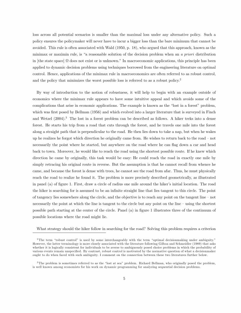
reach the road to realize he found it. The problem is more precisely described geometrically, as illustrated

in panel (a) of figure 1. First, draw a circle of radius one mile around the hiker’s initial location. The road

the hiker is searching for is assumed to be an infinite straight line that lies tangent to this circle. The point

of tangency lies somewhere along the circle, and the objective is to reach any point on the tangent line — not

necessarily the point at which the line is tangent to the circle but any point on the line — using the shortest

possible path starting at the center of the circle. Panel (a) in figure 1 illustrates three of the continuum of

possible locations where the road might lie.

What strategy should the hiker follow in searching for the road? Solving this problem requires a criterion

2The term “robust control” is used by some interchangeably with the term “optimal decisionmaking under ambiguity.”

However, the latter terminology is more closely associated with the literature following Gilboa and Schmeidler (1989) that asks

whether it is logically consistent for individuals to be averse to ambiguously posed choice problems in which the probability of

various events remain unspecified. By contrast, robust control is motivated by the normative question of what a decisionmaker

ought to do when faced with such ambiguity. I comment on the connection between these two literatures further below.

3The problem is sometimes referred to as the “lost at sea” problem. Richard Bellman, who originally posed the problem,

is well known among economists for his work on dynamic programming for analyzing sequential decision problems.

5

to determine what constitutes the “best” possible strategy. In principle, if the hiker knew his propensity to

wake up in a particular orientation relative to the direction he travelled from, he could assign a probability

that his starting point lies in any given direction. In that case, he could pick the strategy that minimizes

the expected distance he would need to reach the main road. But what if the hiker has no good notion

of his propensity to lie down in a particular orientation or the odds that he didn’t turn in his sleep? One

possibility, to which I shall return below, is to assume all locations are equally likely and choose the path that

minimizes the expected distance to reach any point along the road. While this restriction seems natural

in that it does not favor any one direction over another, it still amounts to imposing beliefs about the

likelihood of events the hiker cannot fathom. After all, it is not clear why assuming that the road is equally

likely to lie in any direction should be a good model of the physical problem that describes how likely the

hiker is to rotate a given amount in his sleep.

Bellman (1956) proposed an alternative criterion for choosing the strategy that does not require assigning

any distribution to the location of the road. He suggested choosing the strategy that minimizes the amount

of walking required to ensure reaching the road regardless of where it is located. That is, for any strategy, we

can compute the longest distance one would have to walk to make sure he reaches the main road regardless

of which direction the road lies. It will certainly be possible to search for the road in a way that ensures

reaching the road after a finite amount of hiking: For example, the hiker could walk one mile in any

particular direction, and then, if he didn’t reach the road, turn to walk along the circle of radius one mile

around his original location. This strategy ensures he will eventually find the road. Under this strategy,

the most the hiker would ever have to walk to find the road is 1 + 2 ≈ 728 miles. This is the amount hewould have to walk if the road was a small distance from where he ended up after walking one mile out from

his original location, but the hiker unfortunately chose to turn in the opposite direction when he started

to traverse the circle. Bellman suggested choosing the strategy for which the maximal distance required to

guarantee reaching the road is shortest. The appeal of this rule is that it requires no more walking than

is absolutely necessary to reach the road. While other criteria have been proposed for the lost in a forest

problem, many have found the criterion of walking no more than is absolutely necessary to be intuitively

appealing. But this is precisely the robust control approach. The worst-case scenario for any search strategy

involves exhaustively searching through every wrong location before reaching the true location. Bellman’s

suggestion thus amounts to using the strategy whose worst-case scenario requires less walking than the

worst-case scenario of any other strategy. In other words, the “best” strategy is the one that minimizes the

amount of distance the hiker would need to run through the gamut of all possible locations for the road.

Although Bellman (1956) first proposed this rule as a solution to the lost in a forest problem, it was Isbell

(1957) who derived the strategy that meets this criterion. Readers who are interested in the derivation of

the optimal solution are referred to Isbell’s original piece. It turns out that it is possible to search for the

6

road in a way that requires walking no more than approximately 640 miles, along the path illustrated by

the heavy line in panel (b) of figure 1. The idea is that by deviating from the circle and possibly reaching the

road at a different spot from where the hiker originally left, one can improve upon the strategy of tracking

the circle until reaching the road just at the point in which it lies tangent to the circle of radius one mile

around the hiker’s starting point.

An important feature of the lost in a forest problem is that the set of possibilities the hiker must consider

in order to compute the worst-case scenario for each policy is an objective feature of the environment: The

main road must lie somewhere along a circle of radius one mile around where the hiker fell asleep, we just

don’t know where. By contrast, in most macroeconomic applications, there is no objective set of models

an agent should use in computing the worst-case scenario. Rather, the set of models agents can consider

is typically derived by first positing some benchmark model and then considering all the models that are

“close” in the sense that they imply a distribution for the endogenous variables of the model that is not

too different from the distribution of these same variables under the benchmark model — often taken to be

the entropy distance between the two distributions. Alternatively, agents can contemplate any conceivable

model, but relying on a model that is further away from the benchmark model incurs a penalty in proportion

to the entropy distance between that model and the benchmark one.4 Thus, in contrast with the lost in

a forest problem, economic applications often involve some arbitrariness in that the set of scenarios over

which the worst-case scenario is calculated involves terms that are not tied down by theory — a benchmark

model and a maximal distance or a penalty parameter that governs how far the models agents contemplate

can be from this benchmark. One way of making these choices less arbitrary is to choose the maximal

distance or penalty parameter in such a way that policymakers will not consider models that given the

relevant historical time-series data can be easily rejected statistically in favor of the benchmark model.

The robust strategy is viewed by many mathematicians as a satisfactory solution for the lost in a forest

problem. However, just as economists have critiqued the use of robustness in economics, one can find fault

with this search strategy. The remainder of this section reviews the debate over whether robustness is an

appropriate criterion for coping with uncertainty, using the lost in a forest problem for illustration.

One critique of robustness holds that the robust policy is narrowly tailored to do well in particular

scenarios rather than in most scenarios. This critique is sometimes described as “perfection being the

enemy of the good”: The robust strategy is chosen because it does well in the worst-case scenario, even if

that scenario is unlikely and even if the same strategy performs much worse than alternative strategies in

most, if not all, remaining scenarios. Svennson (2007) conveys this critique as follows: “If a Bayesian prior

probability measure were to be assigned to the feasible set of models, one might find that the probability

4Hansen and Sargent (2008) refer to these two approaches as constraint preferences and multiplier preferences, respectively.

7

assigned to the models on the boundary are exceedingly small. Thus, highly unlikely models can come to

dominate the outcome of robust control.”5 This critique can be illustrated using the lost in a forest problem.

In that problem, the worst-case scenario for any search strategy involves guessing each and every one of

the wrong locations first before finding the road. Arguably, guessing wrong at each possible turn is rather

unlikely, yet the robust policy is tailored to this scenario, and the hiker does not take advantage of shortcuts

that allow him to search through many locations without having to walk a great distance.

The main problem with this critique is that the original motivation for using the robustness criterion to

design policy is that the policymaker cannot assign a probability distribution to the scenarios he considers.

Absent such a distribution, one cannot argue that the worst-case scenario is unlikely. That is, there is no

way to tell whether the Bayesian prior probability measure Svennson alludes to is reasonable. One possible

response is that even absent an exact probability distribution, we might be able to infer from common

experience that the worst-case scenario is not very likely. For example, returning to the example of the lost

in a forest problem, we do not often run through all possibilities before we find what we are searching for,

so the worst-case scenario should be viewed as remote even without attaching an exact probability to this

event. But such intuitive arguments are tricky. Consider the popularity of the adage known as Murphy’s

Law, which states that whatever can go wrong will go wrong. The fact that people view things going wrong

at every turn as a sufficiently common experience to be humorously elevated to the level of a scientific law

suggests they might not view looking through all of the wrong locations first as such a remote possibility.

Even if similar events have proven to be rare in the past, there is no objective way to assure a person who

is worried that this time might be different that he should continue to view such events as unlikely.

In addition, in both the lost in a forest problem and in many economic applications, it is not the case that

the robust strategy performs poorly in all scenarios aside from the worst-case one. In general, the continuity

present in many of these models implies that the strategy that is optimal in the worst-case scenario must

be approximately optimal in nearby situations. Although robust policies may be overly perfectionist in

some contexts, in practice they are often optimal in various scenarios rather than just the worst-case one.

Insisting that a policy do well in many scenarios may not even be feasible, since there may be no single

policy that does well in a large number of scenarios. More generally, absent a probability distribution, there

is no clear reason to prefer a strategy that does well in certain states or in a large number of states, since

it is always possible that those states are themselves unlikely.

Setting aside the issue of whether robust control policies are dominated by highly unlikely scenarios,

economists have faulted other features of robustness and argued against using it as a criterion for designing

5A critique along the same spirit is offered in Section 13.4 in Savage (1954), using an example where the minimax policy is

preferable to alternative rules only under a small set of states that collapses to a single state in the limit.

8

macroeconomic policy. For example, Sims (2001) argues that decisionmakers should avoid rules that violate

the sure-thing principle, which holds that if one action is preferred to another action regardless of which

event is known to occur, it should remain preferred if the event were unknown. As is well known, individuals

whose preferences fail to satisfy the sure-thing principle can in principle be talked into entering gambles

known as “Dutch books” they will almost surely lose.6 But the robust control approach violates the sure-

thing principle. Sims instead advocates that policymakers proceed as Bayesians; that is, they should assign

subjective beliefs to the various scenarios they contemplate and then choose the strategy that minimizes

the expected loss according to their subjective beliefs. Proceeding this way ensures that they will satisfy

the sure-thing principle.7 Al-Najjar and Weinstein (2009) describe other anomalies that arise from minimax

behavior, which they find sufficiently compelling that they argue for rejecting preferences that naturally give

rise to such behavior. The Bayesian prescription that Sims advocates as an alternative to robustness seems

particularly natural for the lost in a forest problem, in which the hiker is always free to assume the road is

equally likely to lie in any direction and then choose the search program that minimizes expected walking

distance given this distribution. Indeed, when Bellman (1956) originally posed his problem, he suggested

both minimizing the longest path (minmax) and minimizing the expected path assuming a uniform prior

(min-mean) as possible solutions.

Do the anomalies that Sims and others point out provide sufficient grounds to reject robustness as

a suitable criterion for choosing policy? As Siniscalchi (2009) notes in his discussion of Al-Najjar and

Weinstein (2009), “there is no fundamental canon of rationality according to which every decisionmaker

should feel similarly uncomfortable” with the implications of minimax strategies. Ultimately, whether one

feels uncomfortable with these implications and prefers to act like a Bayesian is a matter of taste.8 Indeed,

there is some evidence that distaste for the Bayesian prescription advocated by Sims is quite common in

6See, for example, Yaari (1998).

7 Sims (2001) goes on to argue that while robust control is an inappropriate policy recommendation, it might still aid

policymakers who rely on simple procedural rules to guide their decisions rather than explicit optimization. The idea is to

back out what beliefs would justify using the robust strategy, and then reflect on whether these beliefs seem reasonable. As

Sims (2001, p. 52) notes, deriving the robust strategy “may alert decision-makers to forms of prior that, on reflection, do

not seem far from what they actually might believe, yet imply decisions very different from that arrived at by other simple

procedures.” Interestingly, Sims’ prescription cannot be applied to the lost in a forest problem: There is no distribution over

the location of the road for which the minimax path minimizes expected distance. However, the lost in a forest problem offers

an analogous interpretation consistent with Sims’ view. Suppose that the cost of hiking can increase nonlinearly with effort.

In that case, the hiker can ask what cost functions would support the minimax algorithm as a solution to the problem of

minimizing expected effort, assuming the location of the road is distributed uniformly. This can alert him to paths that are

different from mechanical search algorithms he already contemplated that were not derived from his true cost of effort, and to

make him reflect on whether the cost functions that favor the minimax path seem reasonable.

8On this point, note that Yaari (1998) shows that expected utility preferences can also be subject to certain types of Dutch

book manipulation. Rejecting minimax rules on the grounds that they allow for Dutch books while advocating alternative

rules that allow for other types of Dutch books must therefore reflect a subjective distaste for certain types of Dutch books.

But more generally, even if only minimax preferences allowed for Dutch books, the point is that if a policymaker who was

made aware of this vulnerability preferred to stick to his original decision, we could not fault him for these preferences.

9

practice. Take the “Ellsberg paradox” laid out in Ellsberg (1961). This paradox is based on a thought

experiment in which people are asked to choose between a lottery with a known probability of winning

and another lottery featuring identical prizes but with an unknown probability of winning. Ellsberg argued

that most people would not behave as if they assigned a fixed subjective probability to the lottery whose

probability of winnings they did not know, and would instead be averse to participating in a lottery that was

ambiguously specified. In support, he cites several prominent economists and decision theorists to whom

he presented his thought experiment.9 Subsequent researchers who conducted experiments offering these

choices to real-life test subjects, starting with Becker and Brownson (1964), confirmed that people often

fail to behave in accordance with Sims’ prescription of adopting a Bayesian prior. Another example of the

limited appeal of Bayesian decision rules is the aforementioned popularity of Murphy’s Law. A believer in

Murphy’s Law would approach the lost in a forest problem expecting that they are cursed, so that they

will always start their search in the worst possible location. But this implies the location of the road would

depend on where they choose to search, which is inconsistent with assigning a subjective distribution to

the location of the road. Thus, anyone who finds Murphy’s Law appealing would be uncomfortable with

imposing subjective beliefs over the location of the road. Since any recommendation on policy must respect

the policymaker’s tastes, we cannot objectively fault decisionmakers for not behaving like Bayesians.

Note that not all of those who have criticized the robustness criterion have advocated for Bayesian rules.

For example, Savage (1951) argued that the minimax rule is unduly pessimistic, and offered an alternative

approach that has come to be known as “minimax regret.” This view argues for choosing not the policy

that maximizes the lowest possible payoff that could ever be achieved under any conceivable scenario, but

the policy that minimizes the largest possible regret, defined as the difference between the payoff under a

given policy in a given state of the world and the payoff that would have been optimal to pursue in that

state. In other words, a policy should seek to minimize losses relative to what could have been achieved.10

This alternative approach has not been used in macroeconomic applications, but has been used in other

economic applications, for example, in Manski (2004). Such applications are surveyed in Manski (2010),

who considers decision problems where an uncertain decisionmaker must choose an appropriate treatment

rule for a population that may respond differently to different treatments. Manski notes several features

of the minmax-regret approach that differ from the recommendations of either the minmax or Bayesian

approach. Unfortunately, little is known as to whether minimax regret exhibits similarly appealing features

9Ellsberg (1961, p. 655-6) cites these reactions as reflecting the spirit of Paul Samuelson’s reply when confronted with the

fact that his preferences were at odds with certain conventional axioms on preferences: “I’ll satisfy my preferences. Let the

axioms satisfy themselves.” Interestingly, Ellsberg cites Samuelson as one who reported that he would not violate the Savage

axioms when asked about the thought experiment concerning the two lotteries.

10For the lost in a forest problem, the optimal policy given a specific location for the road entails walking exactly one mile

back to the hiker’s starting location. In this case, the policy that minimizes regret turns out to be identical to the one that

minimizes the loss from the worst-case outcome. But the two criterion often lead to different policy recommendations.

10

in macroeconomic applications that involve meeting targets as opposed to assigning treatments. Again,

though, any preference for minimax regret is a matter of subjective tastes, just as with the preference for

Bayesian decision rules.

The theme that runs through the discussion thus far is that if decisionmakers cannot assign probabilities

to scenarios they are uncertain about, there is no inherently correct criterion on how to choose a policy. As

Manski (2000, p. 421) put it, “there is no compelling reason why the decision maker should or should not

use the maximin rule when [the probability distribution] is a fixed but unknown objective function. In this

setting, the appeal of the maximin rule is a personal rather than normative matter. Some decision makers

may deem it essential to protect against worst-case scenarios, while others may not.” Thus, one can point to

unappealing elements about robust control, but these do not definitively rule out this approach. What, then,

is the appeal of robustness that defenders point to? Aside from the intuitive appeal some find in minimizing

risk exposure, proponents of robustness often cite the work on ambiguity aversion, starting with the work

of Gilboa and Schmeidler (1989), as motivation for robustness.11 The latter literature is concerned not with

the normative question of what a decisionmaker should do if he does not know the probability associated

with various relevant scenarios, but with why people often seem averse to situations in which they do not

know the probabilities of various outcomes. More precisely, this literature asks whether there exist coherent

preferences over “acts” in the sense of Savage (1954) that are consistent with preferring clearly posed choice

problems to ambiguously posed ones. Savage defined an “act” as a detailed description of the outcomes

that would occur in every possible state of the world without any reference to the probability these states

will be realized. Gliboa and Schmeidler asked if there are preferences that would tend to favor scenarios in

which the probabilities of final outcomes are clearly stipulated over scenarios in which the probabilities of

final outcomes are not clearly stipulated. For example, could individuals systematically prefer an act where

in each state of the world the individual is offered the same lottery with known odds of winning each prize

to an act where the prizes and odds of winning vary across states, so the odds of winning a particular prize

depends on one’s subjective perceptions of a given state occurring? Some of the preference specifications

that can generate ambiguity aversion imply the agent behaves as if he contemplated a set of subjective

probability distributions over the different states, and then chose the act that guaranteed the highest worst

case expected utility over these distributions, that is, the strategy that was robust to the set of subjective

beliefs he entertains. These preferences can rationalize why people would appear to choose strategies that

are robust to the models they are subjectively willing to contemplate.

Of course, just as the appeal of Sims’ directive to accept the sure-thing principle amounts to a matter

of taste rather than rationality, there is no compelling justification for why a decisionmaker ought to

11Gilboa and Schmeidler (1989) consider only static decision problems. Various authors have since worked on extending

their analysis to dynamic decision problems. See, for example, Epstein and Schneider (2003), Maccheroni, Marinacci, and

Rustichini (2006), and Strzalecki (2009).

11

find compelling the particular axiomatic restrictions on preferences that give rise to minimax behavior.

Ultimately, the aforementioned literature only shows that there exist coherent preferences that justify such

decisions, implying that minimax behavior does not rest on logical contradictions. But this literature

does not argue that these preferences are somehow natural, nor do they offer empirical evidence that

these preferences are common. Instead, these papers largely appeal to the Ellsberg paradox, which can

be reconciled by appealing to preferences that imply subjective multiple priors. But as Al-Najjar and

Weinstein (2009) point out, other explanations for the Ellsberg paradox exist, and the paradox does not by

itself confirm all of the restrictions on preferences needed to give rise to minimax behavior.

Equally important, the axiomatic approach provides a theory of robustness to subjective uncertainty.

That is, it can tell under what conditions decision makers will behave as if they entertain a set of beliefs

regarding the likelihood of various states, and then choose the policies that are robust against this set. But

robust control is typically presented as a theory of what policymakers should do in the face of objective

uncertainty, when they cannot fathom the environment they face. To appreciate this distinction, consider

the lost in a forest problem. The axiomatic approach tells us that if individuals have certain preferences

over proposals for different search algorithms, their decisions can be described as if they had a set of beliefs

over the location of the road, and they chose their strategy to be robust to these beliefs. But there is

no restriction that their preferences must carry over to other decision problems that involve a completely

different set of Savage acts than the original lost in a forest problem. Thus, there is no guarantee that

individuals who follow a minimax rule in the original lost in a forest problem will also follow a minimax rule

if they had to search for a road located two miles away or if they also forgot the distance they originally

hiked before falling asleep. By contrast, Bellman advocated the minimax search strategy as a general rule

for any search problem in which the location of the object is unknown.

In sum, whether policymakers find robustness appealing is subjective. Given the sizable engineering

literature on robust control, the notion of designing systems that minimize the worst-case scenario appears

to have had some appeal among engineers. Interestingly, Murphy’s Law is also an export from the field

of engineering.12 The two observations may be related: If worst-case outcomes are treated as everyday

occurrences, robustness would seem like an appealing criterion. Policymakers who are equally nervous

about worst-case outcomes would presumably like the notion of keeping their risk exposure to a bare

minimum. But less nervous policymakers may find robustness unappealing upon reflection, either because

of its implications in particular models or because it leads to the anomalous results pointed out by detractors.

12According to Spark (2006), the law is named after aerospace engineer Edward Murphy, who complained after a technician

attached a pair of sensors in a precisely incorrect configuration during a crash test Murphy was observing. Engineers on the

team Murphy was working with began referring to the notion that things will inevitably go wrong as Murphy’s Law, and the

expression gained public notoriety after one of the engineers used it in a press conference.

12

4 Robustness and the Brainard Model

Now that I have described what it means for a policy to be robust, I can return to the implications of robust

control for macroeconomic policy. Various authors have solved for the robust policy in particular macro

models, and have carried out comparative static exercises on how the robust policy changes with underlying

features of the model, with the set of models the policymaker entertains, or with the penalty parameter that

governs the disutility from using a model that is different from the benchmark. Not surprisingly, the results

tend to be model-specific, and there are few general results. This is also true for the literature on optimal

policy under uncertainty in the Brainard tradition, which assumes policymakers are uncertain about some

parameters but still know the distribution. For example, Chow (1973) finds few general results when he

considers a broader model that encompasses Brainard’s framework.

However, early applications of robustness did have one result in common: In all of these applications,

the robust policy tended to contradict the attenuation result in Brainard’s model, and instead implied

that uncertain policymakers should react more aggressively to news than they would in the absence of

uncertainty. Examples of this result include Sargent (1999), Stock (1999), Tetlow and von zur Muehlen

(2001), Giannoni (2002), and Onatski and Stock (2002). These findings were sometimes interpreted to

mean that concern for robustness leads to more aggressive policy.13 In this section, my aim is to dispel this

interpretation. In particular, I argue that the lack of attenuation is not driven by concern for robustness per

se, but by the environments these early papers considered. When we consider the implications of robustness

in the same environment that Brainard considered, we obtain similar results to his.14

Consider the Brainard model above, but suppose now that the policymaker no longer knows the distribu-

tion of all of the parameters that he is uncertain about. More precisely, suppose the variable to be targeted,

, is still determined by (2):

= − ( + ) + (5)

Since the attenuation result only arises when the policymaker is uncertain about , I will continue to

assume the policymaker knows the distribution of for simplicity. By contrast, I assume the policymaker

only knows that the support of is restricted to some interval [ ] that includes 0, that is, 0 , and

does not know its distribution. Thus, the effect of on can be less than, equal to, or higher than , but

the policymaker cannot ascribe probabilities to these events.15

13For example, Bernanke (2007) notes: “The concern about worst-case scenarios emphasized by the robust-control approach

may likewise lead to amplification rather than attenuation in the response of the optimal policy to shocks.”

14A similar point was made by Onatski (1999), who considers a closely related example to the one I discuss in this section.

15The case where a decisionmaker is uncertain about the value of one or more parameters in a model is known as structured

13

The robust control approach in this environment can be viewed as a two-step process. First, for each

value of , we compute its worst-case scenario over all values ∈ [ ], or the largest expected loss thepolicymaker could incur. Define this expected loss as (); that is,

() ≡ max∈[]

£2¤= max

∈[]

n(− ( + ))

2+ 2

o (6)

Second, we choose the policy that implies the smallest value for (). The robust strategy is defined as

the value of that solves min (); that is,

min

max∈[]

n(− ( + ))

2+ 2

o (7)

Below, I describe the solution to this problem and provide some intuition for it. For a rigorous derivation,

see Barlevy (2009). It turns out that the robust policy hinges on the lowest value that can assume. If

≤ −, so the coefficient + can be either positive or negative, the solution to (7) is given by

= 0

If instead −, so the policymaker is certain that the coefficient + is positive but is unsure of its

exact value, the solution to (7) is given by

=

+ (+ ) 2 (8)

Thus, if the policymaker knows the sign of the effect of on , he should respond to changes in in a way

that depends on the extreme values can assume, that is, the endpoints of the interval [ ]. But if the

policymaker is unsure about the sign of the effect of policy on , he should not respond to at all.16

To better understand why concerns for robustness imply this rule, consider first the result that if the

policymaker is uncertain about the sign of + , he should altogether abstain from responding to . This

is related to Brainard’s (1967) attenuation result: There is an inherent asymmetry in that a passive policy

where = 0 leaves the policymaker unexposed to risk from , while a policy that sets 6= 0 leaves him

exposed to such risk. When the policymaker is sufficiently concerned about this risk, which turns out to

hinge on whether he knows the sign of the coefficient on , he is better off resorting to a passive policy that

uncertainty. Unstructured uncertainty refers to the case where the decisionmaker is unsure about the probability distribution

for the endogenous variables in the model, and considers any distribution that is some entropy distance from a benchmark

model. The original finding that robust policy tends to be aggressive was demonstrated for both types of uncertainty.

16 Interestingly, Kocherlakota and Phelan (2009) also provide an example where doing nothing is the minmax solution to

a policy problem. They show that if policymakers rely on an interventionist mechanism, there is an environment in which

intervention plays no useful role, since it does not allow the policymaker to achieve a superior outcome, but it admits an

additional equilibrium that yields an inferior outcome. Thus, an interventionist mechanism is more vulnerable to bad outcomes

than a mechanism that does nothing. The example here yields a similar outcome, but does not involve multiple equilibria.

14

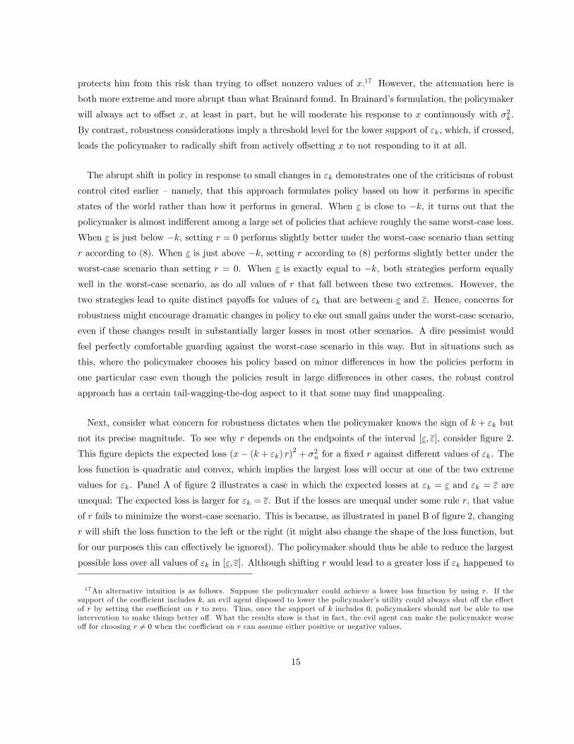
protects him from this risk than trying to offset nonzero values of .17 However, the attenuation here is

both more extreme and more abrupt than what Brainard found. In Brainard’s formulation, the policymaker

will always act to offset , at least in part, but he will moderate his response to continuously with 2.

By contrast, robustness considerations imply a threshold level for the lower support of , which, if crossed,

leads the policymaker to radically shift from actively offsetting to not responding to it at all.

The abrupt shift in policy in response to small changes in demonstrates one of the criticisms of robust

control cited earlier — namely, that this approach formulates policy based on how it performs in specific

states of the world rather than how it performs in general. When is close to −, it turns out that thepolicymaker is almost indifferent among a large set of policies that achieve roughly the same worst-case loss.

When is just below −, setting = 0 performs slightly better under the worst-case scenario than setting according to (8). When is just above −, setting according to (8) performs slightly better under theworst-case scenario than setting = 0. When is exactly equal to −, both strategies perform equally

well in the worst-case scenario, as do all values of that fall between these two extremes. However, the

two strategies lead to quite distinct payoffs for values of that are between and . Hence, concerns for

robustness might encourage dramatic changes in policy to eke out small gains under the worst-case scenario,

even if these changes result in substantially larger losses in most other scenarios. A dire pessimist would

feel perfectly comfortable guarding against the worst-case scenario in this way. But in situations such as

this, where the policymaker chooses his policy based on minor differences in how the policies perform in

one particular case even though the policies result in large differences in other cases, the robust control

approach has a certain tail-wagging-the-dog aspect to it that some may find unappealing.

Next, consider what concern for robustness dictates when the policymaker knows the sign of + but

not its precise magnitude. To see why depends on the endpoints of the interval [ ], consider figure 2.

This figure depicts the expected loss (− ( + ) )2+ 2 for a fixed against different values of . The

loss function is quadratic and convex, which implies the largest loss will occur at one of the two extreme

values for . Panel A of figure 2 illustrates a case in which the expected losses at = and = are

unequal: The expected loss is larger for = . But if the losses are unequal under some rule , that value

of fails to minimize the worst-case scenario. This is because, as illustrated in panel B of figure 2, changing

will shift the loss function to the left or the right (it might also change the shape of the loss function, but

for our purposes this can effectively be ignored). The policymaker should thus be able to reduce the largest

possible loss over all values of in [ ]. Although shifting would lead to a greater loss if happened to

17An alternative intuition is as follows. Suppose the policymaker could achieve a lower loss function by using . If the

support of the coefficient includes , an evil agent disposed to lower the policymaker’s utility could always shut off the effect

of by setting the coefficient on to zero. Thus, once the support of includes 0, policymakers should not be able to use

intervention to make things better off. What the results show is that in fact, the evil agent can make the policymaker worse

off for choosing 6= 0 when the coefficient on can assume either positive or negative values.

15

equal , since the goal of a robust policy is to minimize the largest possible loss, shifting in this direction

is desirable. Robustness concerns would therefore lead the policymaker to adjust until the losses at the

two extreme values were balanced, so that the loss associated with the policy being maximally effective is

exactly equal to the loss associated with the policy being minimally effective.

When there is no uncertainty, that is, when = = 0, the policymaker would set = , since this

would set exactly equal to its target. When there is uncertainty, whether the robust policy will respond

to more or less aggressively than this benchmark depends on how the lower and upper bounds are located

relative to 0. If the region of uncertainty is symmetric around 0 so that = −, uncertainty has no effecton policy. To see this, note that if we were to set = , the expected loss would reduce to ()

22+2,

which is symmetric in . Hence, setting to offset would naturally balance the loss at the two extremes.

But if the region of uncertainty is asymmetric around 0, setting = would fail to balance the expected

losses at the two extremes, and would have to be adjusted so that it either responds more or less to

than in the case of complete certainty. In particular, the response to will be attenuated if −, thatis, if the potential for an overly powerful stimulus is greater than the potential for stimulus that is far too

weak, and this response will be amplified in the opposite scenario.

This result begs the question of when the support for will be symmetric or asymmetric in a particular

direction. If the region of uncertainty is constructed using past data on , , and , any asymmetry would

have to be driven by differences in detection probabilities across different scenarios — for example, if it is

more difficult to detect when its value is large than when it is small. This may occur if the distribution of

were skewed in a particular direction. But if the distribution of were symmetric around 0, policymakers

who rely on past data should find it equally difficult to detect deviations in either direction, and the robust

policy would likely react to shocks in the same way as if were known with certainty.

The above example shows that the robustness criterion does not inherently imply that policy should be

more aggressive in the face of uncertainty. Quite to the contrary, the robust policy exhibits a more extreme

form of the same attenuation principle that Brainard demonstrated, for essentially the same reason: The

asymmetry between how passive and active policies leave the policymaker exposed to risk tends to favor

passive policies. More generally, whether uncertainty about the economic environment leads to attenuation

or more aggressive policy depends on asymmetries in the underlying environment. If the policymaker

entertains the possibility that policy can be far too effective but not that it will be very ineffective, he will

naturally tend to attenuate his policy. But if his beliefs are reversed, he will tend to magnify his response

to news about potential deviations from the target level.18

18Rustem, Wieland, and Zakovic (2007) also consider robust control in asymmetric models, although they do not discuss

the implications of these asymmetries for attenuation.

16

5 Robustness and Aggressive Rules

Given that robustness considerations do not necessarily imply more aggressive policies, which features of

the macro models that were used in early applications of robust control account for the finding that robust

policies tend to be more aggressive? The papers cited earlier consider different models, and their results

are not driven by one common feature. To give some flavor of why some factors may lead robust policies

to be aggressive, I now consider two simplified examples inspired by these papers. The first assumes the

policymaker is uncertain about the persistence of shocks, following Sargent (1999). The second assumes

the policymaker is uncertain about the tradeoff between competing objectives, following Giannoni (2002).

I show that both features can tilt the robust policy toward reacting more aggressively to incoming news.

5.1 Uncertain persistence

One of the first to argue that concerns for robustness could dictate more aggressive policy was Sargent

(1999). Sargent asked how optimal policy would be affected in a particular model when we account for the

possibility that the model is misspecified — and especially the possibility that specification errors are serially

correlated. To gain some insight on the implications of serially correlated shocks, consider the following

extension of the Brainard model in which the policymaker attempts to target only one variable.19

Let denote the value at date of the variable that the policymaker wishes to target to 0. As in (1), I

assume is linear in the policy variable and in an exogenous shock term :

= −

I now no longer assume the policymaker is uncertain about the effect of his policy on . As such, it will

be convenient to normalize to 1. However, I now assume the policymaker is uncertain about the way

is correlated over time. That is, suppose follows the AR(1) process

= −1 +

where are independent and identically distributed over time with mean 0 and variance 2, and captures

the autocorrelation of . At each date , the policymaker can observe −1 and condition his policy on its

realization. However, he must set before observing . His uncertainty about is due to two different

factors. First, I assume he does not know at the time he chooses his policy. Second, to capture uncertainty

19Sargent assumed the policymaker cares about both inflation and unemployment, following the model he was discussing.

Here, I continue to assume the policymaker cares about only one target. But my objective is not to replicate Sargent’s results.

Rather, it is to illustrate why a concern that shocks are persistent can lead to robust policies that tend to be aggressive.

17

about the persistence of variables over which the policymaker is uncertain, I assume the policymaker does

not know the autocorrelation coefficient that governs how −1 affects .

Suppose the policymaker discounts future losses at rate 1 so that his expected loss is given by

" ∞X=0

2

#=

" ∞X=0

( − )2

#

If the policymaker knew with certainty, his optimal strategy would be to set = [|−1] = −1.

But in line with the notion that the policymaker remains uncertain about the degree of persistence, suppose

he only knows that falls in some interval£ ¤. Let ∗ denote the midpoint of this interval:

∗ =¡+

¢2

To emphasize asymmetries inherent to the loss function as opposed to the region of uncertainty, suppose

the interval of uncertainty is symmetric around the certainty benchmark. An important and empirically

plausible assumption in what follows is that ∗ 0; that is, the beliefs of the monetary authority are

centered around the possibility that shocks are positively correlated.

Once again, we can derive the robust strategy in two steps. First, for each rule , define () as the

biggest loss possible among the different values of ; that is,

() = max∈[]

" ∞X=0

2

#

We then choose the policy rule that minimizes (); that is, we solve

min

max∈[]

" ∞X=0

2

# (9)

Following Sargent (1999), I assume the policymaker is restricted in the type of policies he can carry out:

He must choose a rule of the form = −1, where is a constant that cannot vary over time. This

restriction is meant to capture the notion that the policymaker cannot learn about the parameters over

which he is uncertain and then change the way policy reacts to information as he observes over time

and potentially infer . I further assume the expectation in (9) is the unconditional expectation of future

losses; that is, the policymaker calculates his expected loss from the perspective of date 0. To simplify the

calculations, I assume 0 is drawn from the stationary distribution for .

The solution to (9), subject to the constraint that = −1, is derived in Barlevy (2009). The key

result is that as long as ∗ 0, the robust policy would set to a value in the interval that is strictly greater

than the midpoint ∗. In other words, starting with the case in which the policymaker knows = ∗, if

we introduce a little bit of uncertainty in a symmetric fashion so that the degree of persistence can deviate

18

equally in either direction, the robust policy would react more to a change in −1 in the face of uncertainty

than it would react to such a change if the degree of persistence were known with certainty.

To understand this result, suppose the policymaker set = ∗. As in the previous section, the loss

function is convex in , so the worst-case scenario will occur when assumes one of its two extreme values,

that is, when either = or = . It turns out that when = ∗, setting = imposes a bigger cost on the

policymaker than setting = . Intuitively, for any given , setting = ∗ will imply = (−∗)−1+.

The expected deviation of from its target given −1 will have the same expected magnitude in both

cases; that is, |(− ∗)−1| will be the same when = and = , given£ ¤is symmetric around ∗.

However, the process will be more persistent when is higher, and so deviations from the target will be

more persistent when = than when = . More persistent deviations imply more volatile and hence

a larger expected loss. Since the robust policy tries to balance the losses at the two extreme values of ,

the policymaker should choose a higher value for to reduce the loss when = .

The basic insight is that, while the loss function for the policymaker is symmetric in around = 0, if we

focus on an interval that is centered around positive values of , the loss function will be asymmetric. This

asymmetry will tend to favor policies that react more to past shocks. In fact, this feature is not unique to

policies guided by robustness. If we assumed the policymaker assigned a symmetric distribution to values of

in the interval£ ¤and acted to minimize his expected losses, the asymmetry in the loss function would

continue to imply that the value of that solves min

hX∞

=0 (−1 − −1 + )

2iwill exceed ∗.

Hence, the feature responsible for the aggressiveness of the robust policy is not disproportionate attention

to worst-case scenarios, since even if the policymaker assigned small probabilities to extreme values of , he

might still respond aggressively to past shocks given such beliefs. Rather, because more persistent shocks

create bigger losses than less persistent shocks, policymakers will want to minimize the damage in the event

that shocks are persistent. As in the Brainard model, what tilts policy away from its certainty benchmark

is an underlying asymmetry that favors certain types of policies over others.

5.2 Uncertain tradeoff parameters

Next, I turn to the Giannoni (2002) model. Giannoni focused on the case where policymakers are uncertain

about the parameters in the underlying model the policymaker believes, specifically the parameters that

dictate the effect of shocks on the endogenous variables in the model. If policymakers wish to target

more than one of these variables, this can make them uncertain about the tradeoff between meeting their

competing objectives, which in Giannoni’s framework turns out to favor more aggressive policies. Up to

now, I have conveniently assumed policymakers were only interested in targeting a single variable. However,

tradeoffs in trying to target multiple variables can be important in designing robust policy, and so it is worth

19

exploring a simplified example to illustrate some of these effects.

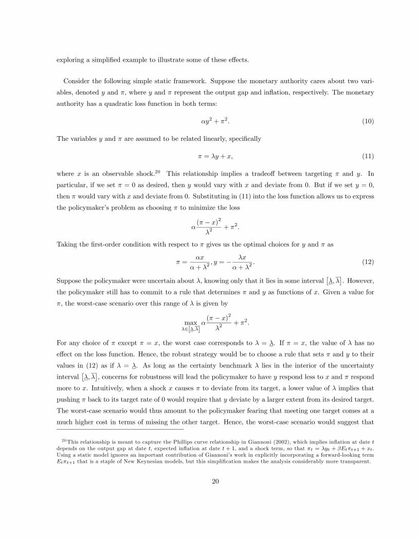
Consider the following simple static framework. Suppose the monetary authority cares about two vari-

ables, denoted and , where and represent the output gap and inflation, respectively. The monetary

authority has a quadratic loss function in both terms:

2 + 2 (10)

The variables and are assumed to be related linearly, specifically

= + (11)

where is an observable shock.20 This relationship implies a tradeoff between targeting and . In

particular, if we set = 0 as desired, then would vary with and deviate from 0. But if we set = 0,

then would vary with and deviate from 0. Substituting in (11) into the loss function allows us to express

the policymaker’s problem as choosing to minimize the loss

( − )

2

2+ 2

Taking the first-order condition with respect to gives us the optimal choices for and as

=

+ 2 = −

+ 2 (12)

Suppose the policymaker were uncertain about , knowing only that it lies in some interval£

¤. However,

the policymaker still has to commit to a rule that determines and as functions of . Given a value for

, the worst-case scenario over this range of is given by

max∈[]

( − )

2

2+ 2

For any choice of except = , the worst case corresponds to = . If = , the value of has no

effect on the loss function. Hence, the robust strategy would be to choose a rule that sets and to their

values in (12) as if = . As long as the certainty benchmark lies in the interior of the uncertainty

interval£

¤, concerns for robustness will lead the policymaker to have respond less to and respond

more to . Intuitively, when a shock causes to deviate from its target, a lower value of implies that

pushing back to its target rate of 0 would require that deviate by a larger extent from its desired target.

The worst-case scenario would thus amount to the policymaker fearing that meeting one target comes at a

much higher cost in terms of missing the other target. Hence, the worst-case scenario would suggest that

20This relationship is meant to capture the Phillips curve relationship in Giannoni (2002), which implies inflation at date

depends on the output gap at date , expected inflation at date + 1, and a shock term, so that = + +1 + .

Using a static model ignores an important contribution of Giannoni’s work in explicitly incorporating a forward-looking term

+1 that is a staple of New Keynesian models, but this simplification makes the analysis considerably more transparent.

20

the policymaker should not try to stabilize too much for fear of missing his target for . Put another way,

the robust policy implies more aggressively stabilizing and less aggressively stabilizing .

Figure 3 illustrates this result graphically. The problem facing the policymaker is to choose a point from

the line given by = + . Ideally, it would like to move toward the origin, where = = 0. Changing

will rotate the line from which the policymaker must choose, as depicted in the figure. A lower value of

corresponds to a flatter curve. Given the policymaker prefers to be close to the origin, a flatter curve leaves

the policymaker with distinctly worse options that are farther from the origin, since one can show that

the policymaker would only choose points in the upper left quadrant of the figure. This explains why the

worst-case scenario corresponds to the flattest curve possible. If we assume the policymaker must choose his

relative position on the line before knowing the slope of the line (that is, before knowing ), then the flatter

the line could be, the greater his incentive will be to locate close to the -axis rather than risk deviating

from his target on both variables, as indicated by the path with the arrow. This explains why he will act

more aggressively to isolate the effects of on .

Robustness concerns thus encourage the policymaker to proceed as if he knew was equal to its lowest

possible value. Note the difference from the two earlier models, in which the robust policy recommended

balancing losses associated with two polar opposite scenarios. Here, the policy equates marginal losses for

a particular risk (the loss from letting deviate a little more from its target and the loss from letting

deviate a little more), namely the risk that will be low so that stabilizing inflation comes at a large cost

of destabilizing output.

6 Conclusion

My objective in this paper was to review the robustness criterion that some macroeconomists have advocated

for designing policy when policymakers are at a loss to assign probabilities to the scenarios they contemplate.

The key theme I have stressed is that in the absence of objective probabilities, there is no right criterion

by which to choose policy. Critics of robust control are really just expressing their own subjective views

about some of the implications of this approach, just as advocates of robust control are expressing their

own subjective views that this approach has some appealing features. While there is no one right answer for

whether robustness is an appropriate criterion for designing policy, even critics of robustness are willing to

acknowledge that deriving the robust policy and understanding its properties can be useful, not necessarily

because policymakers should adopt this policy but because solving for this rule can alert policymakers to

where their policies might go amiss and whether acting to minimize the potential for losses is costly. Since

the exact features of robust policies will depend on the underlying environment, typically one would have to

solve for the minimax policy in each application rather than rely on general results on the nature of robust

21

policy rules. Indeed, one of the points of this survey was that concern for robustness does not inherently

contradict the attenuation principle derived by Brainard (1967), contrary to what some have inferred based

on the results that emerged from the particular models used in early applications of robust control.

My survey focused exclusively on the normative question of how macroeconomic policymakers should

behave when they are uncertain about the environment they face. However, equally important questions

left out from this survey hinge on whether policymakers and agents do in fact exhibit a preference for

robustness and choose policies this way. For example, Ellison and Sargent (2009) argue that concern for

robustness can help to understand monetary policy and why the Federal Open Market Committee seems to

ignore projections made by their staff even though they know these are good forecasts of future economic

conditions. In addition, various authors have investigated the nature of optimal policy when private agents

follow robust decision rules, both when policymakers themselves face no uncertainty and when policymakers

are themselves concerned about robustness. Even if there are compelling arguments for why robustness may

not always be desirable, evidence that agents have a taste for robustness may still force policymakers to

take robustness concerns into account when designing macroeconomic policy.

References

[1] Al-Najjar, Nabil and Jonathan Weinstein, 2009, “The Ambiguity Aversion Literature: a Critical As-

sessment” Economics and Philosophy, Vol. 25, No. 03, November 2009, pp. 249-284.

[2] Barlevy, Gadi, 2009. “Policymaking under Uncertainty: Gradualism and Robustness” Economic Per-

spectives, Federal Reserve Bank of Chicago, QII, pp. 38-55.

[3] Becker, Selwyn, and Fred Brownson, 1964, "What Price Ambiguity? Or the Role of Ambiguity in

Decision-making," Journal of Political Economy, Vol. 72, No. 1, February, pp. 62-73.

[4] Bellman, Richard, 1956, "Minimization Problem," Bulletin of the American Mathematical Society, Vol.

62, No. 3, p. 270.

[5] Bernanke, Ben, 2007, “Monetary Policy Under Uncertainty,” speech at the 32nd Annual Economic

Policy Conference, Federal Reserve Bank of St. Louis (via videoconference), October 19, available at

www.federalreserve.gov/newsevents/speech/bernanke20071019a.htm.

[6] Blinder, Alan, 1998. Central Banking in Theory and Practice. Cambridge: MIT Press.

[7] Brainard, William, 1967, "Uncertainty and the Effectiveness of Policy," American Economic Review,

Vol. 57, No. 2, May, pp. 411-425.

22

[8] Caballero, Ricardo and Arvind Krishnamurthy, 2008. “Collective Risk Management in a Flight to

Quality Episode” Journal of Finance, Vol. 63, No. 5, pp. 2195-2236.

[9] Chow, Gregory, 1973. “Effect of Uncertainty on Optimal Control Policies” International Economic

Review, Vol. 14, No. 3, October, pp. 632-645.

[10] Craine, Roger, 1979. “Optimal Monetary Policy with Uncertainty” Journal of Economic Dynamics and

Control, Vol. 1, No. 1, February, pp. 59-83.

[11] Ellison, Martin and Thomas Sargent, 2009. “In Defense of the FOMC” Mimeo, New York University.

[12] Ellsberg, Daniel, 1961, "Risk, Ambiguity, and the Savage Axioms," Quarterly Journal of Economics,

Vol. 75, No. 4, November, pp. 643-669.

[13] Epstein, Larry, and Martin Schneider, 2003, "Recursive Multiple-Priors," Journal of Economic Theory,

Vol. 113, No. 1, November, pp. 1-31.

[14] Finch, Steven, and John Wenzel, 2004, "Lost in a Forest," American Mathematical Monthly, Vol. 111,

No. 8, October, pp. 645-654.

[15] Giannoni, Marc, 2002, "Does Model Uncertainty Justify Caution? Robust Optimal Monetary Policy

in a Forward-Looking Model," Macroeconomic Dynamics, Vol. 6, No. 1, February, pp. 111-144.

[16] Gilboa, Itzhak, and David Schmeidler, 1989, "Maxmin Expected Utility with Nonunique Prior," Journal

of Mathematical Economics, Vol. 18, No. 2, April, pp. 141-153.

[17] Gluss, Brian, 1961, "An Alternative Solution to the ’Lost at Sea’ Problem," Naval Research Logistics

Quarterly, Vol. 8, No. 1, March, pp. 117-121.

[18] Hansen, Lars and Thomas Sargent, 2008, Robustness, Princeton, NJ: Princeton University Press.

[19] Isbell, John, 1957, "An Optimal Search Pattern," Naval Research Logistics Quarterly, Vol. 4, No. 4,

December, pp. 357-359.

[20] Karantounias, Anastasios with Lars Hansen, and Thomas Sargent, 2009. “Managing Expectations and

Fiscal Policy” Mimeo, NYU.

[21] Kocherlakota, Narayana and Chris Phelan, 2009. “On the Robustness of Laissez-faire” Journal of

Economic Theory, Vol. 144, No. 6, November, pp. 2372-87.

[22] Maccheroni, Fabio, Massimo Marinacci, and Aldo Rustichini, 2006, "Dynamic Variational Preferences,"

Journal of Economic Theory, Vol. 128, No. 1, May, pp.4-44.

23

[23] Manski, Charles, 2000, "Identification Problems and Decisions Under Ambiguity: Empirical Analysis

of Treatment Response and Normative Analysis of Treatment Choice," Journal of Econometrics, Vol.

95, No. 2, April, pp. 415-442.

[24] Manski, Charles, 2004, “Statistical Treatment Rules for Heterogeneous Populations” Econometrica,

Vol. 72, No. 4, July, pp. 1221—1246.

[25] Manski, Charles, 2010. “Social Planning Under Ambiguity” Annual Review of Economics.

[26] Onatski, Alexei, 1999. “Minimax Analysis of Model Uncertainty: Comparison to Bayesian Approach,

Worst Possible Economies, and Optimal Robust Monetary Policies” Mimeo, Harvard University.

[27] Onatski, Alexei, and James Stock, 2002, "Robust Monetary Policy Under Model Uncertainty in a Small

Model of the U.S. Economy," Macroeconomic Dynamics, Vol. 6, No. 1, February, pp. 85-110.

[28] Rustem, Berc, Volker Wieland, and Stan Zakovic, 2007, "Stochastic Optimization and Worst-Case

Analysis in Monetary Policy Design," Computational Economics, Vol. 30, No. 4, November, pp. 329-

347.

[29] Sargent, Thomas, 1999, "Comment on ’Policy Rules for Open Economies’ by Laurence Ball," in Mone-

tary Policy Rules, John Taylor (ed.), National Bureau of Economic Research Studies in Business Cycles,

Vol. 31, Chicago: University of Chicago Press, pp. 144-154.

[30] Savage, Leonard, 1951. “The Theory of Statistical Decision” Journal of the American Statistical Asso-

ciation, Vol. 46, No. 253, March, pp. 55-67.

[31] Savage, Leonard, 1954. The Foundations of Statistics, New York: Wiley.

[32] Sims, Christopher, 2001, "Pitfalls of a Minimax Approach to Model Uncertainty," American Economic

Review, Vol. 91, No. 2, May, pp. 51-54.

[33] Siniscalchi, Marciano, 2009. “Two out of Three Ain’t Bad: a Comment on ‘The Ambiguity Aversion

Literature: a Critical Assessment’” Economics and Philosophy, Vol. 25, No. 03, November 2009, pp.

335-356.

[34] Soderstrom, Ulf, 2002. “Monetary Policy with Uncertain Parameters” The Scandinavian Journal of

Economics, Vol. 104, No. 1, March, pp. 125-145.

[35] Spark, Nick, 2006, A History of Murphy’s Law, Los Angeles: Periscope Film.

[36] Stock, James, 1999, "Comment on ’Policy Rules for Inflation Targeting’ by Glenn Rudebusch and

Lars Svensson," in Monetary Policy Rules, John Taylor (ed.), National Bureau of Economic Research

Studies in Business Cycles, Vol. 31, Chicago: University of Chicago Press, pp. 253-259.

24

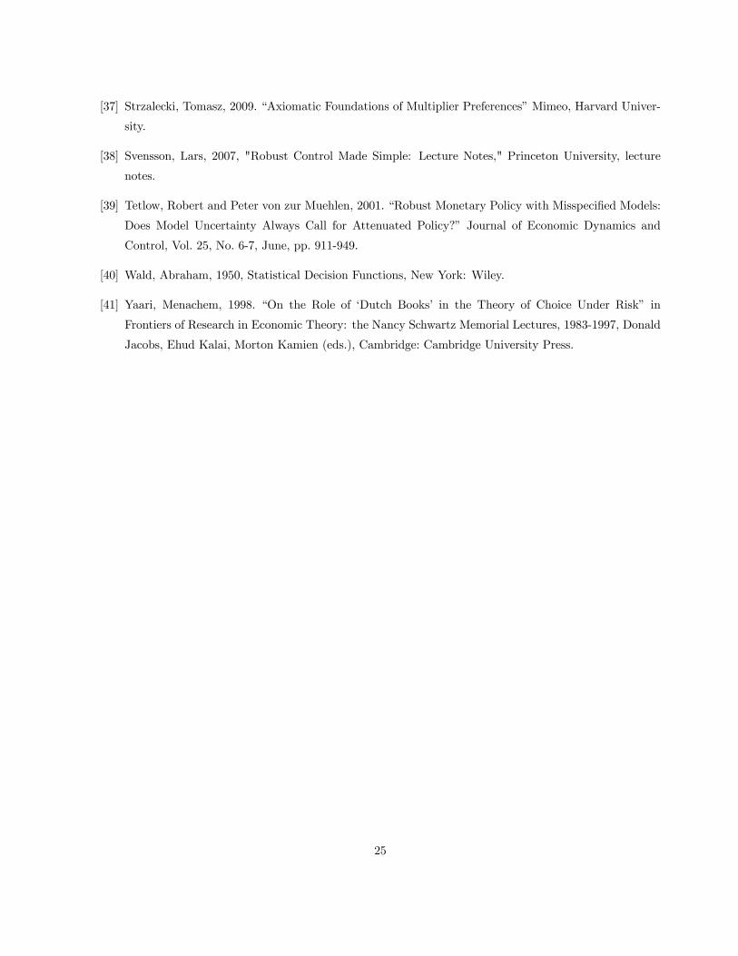
[37] Strzalecki, Tomasz, 2009. “Axiomatic Foundations of Multiplier Preferences” Mimeo, Harvard Univer-

sity.

[38] Svensson, Lars, 2007, "Robust Control Made Simple: Lecture Notes," Princeton University, lecture

notes.

[39] Tetlow, Robert and Peter von zur Muehlen, 2001. “Robust Monetary Policy with Misspecified Models:

Does Model Uncertainty Always Call for Attenuated Policy?” Journal of Economic Dynamics and

Control, Vol. 25, No. 6-7, June, pp. 911-949.

[40] Wald, Abraham, 1950, Statistical Decision Functions, New York: Wiley.

[41] Yaari, Menachem, 1998. “On the Role of ‘Dutch Books’ in the Theory of Choice Under Risk” in

Frontiers of Research in Economic Theory: the Nancy Schwartz Memorial Lectures, 1983-1997, Donald

Jacobs, Ehud Kalai, Morton Kamien (eds.), Cambridge: Cambridge University Press.

25

(a) Graphical representation of the problem

(b) Min‐max path, derived by Isbell (1957)

Figure 1: Graphical Representation of the “Lost in a Forest” Problem

11

1

210⁰

2√3

1√3

30⁰

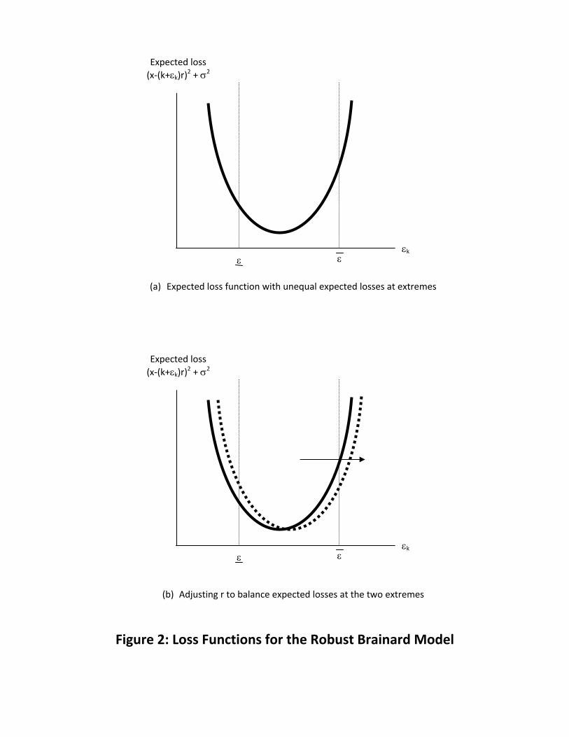
(a) Expected loss function with unequal expected losses at extremes

(b) Adjusting r to balance expected losses at the two extremes

Figure 2: Loss Functions for the Robust Brainard Model

ε ε εk

Expected loss (x‐(k+εk)r)2 + σ2

ε ε εk

Expected loss (x‐(k+εk)r)2 + σ2

Figure 3: Graphical Representation of Uncertain Tradeoffs Model

0

π

y

lower λ

x

higher λ

1

Working Paper Series

A series of research studies on regional economic issues relating to the Seventh Federal Reserve District, and on financial and economic topics.

Risk Taking and the Quality of Informal Insurance: Gambling and Remittances in Thailand WP-07-01 Douglas L. Miller and Anna L. Paulson

Fast Micro and Slow Macro: Can Aggregation Explain the Persistence of Inflation? WP-07-02 Filippo Altissimo, Benoît Mojon, and Paolo Zaffaroni

Assessing a Decade of Interstate Bank Branching WP-07-03 Christian Johnson and Tara Rice

Debit Card and Cash Usage: A Cross-Country Analysis WP-07-04 Gene Amromin and Sujit Chakravorti

The Age of Reason: Financial Decisions Over the Lifecycle WP-07-05 Sumit Agarwal, John C. Driscoll, Xavier Gabaix, and David Laibson

Information Acquisition in Financial Markets: a Correction WP-07-06 Gadi Barlevy and Pietro Veronesi

Monetary Policy, Output Composition and the Great Moderation WP-07-07 Benoît Mojon

Estate Taxation, Entrepreneurship, and Wealth WP-07-08 Marco Cagetti and Mariacristina De Nardi

Conflict of Interest and Certification in the U.S. IPO Market WP-07-09 Luca Benzoni and Carola Schenone

The Reaction of Consumer Spending and Debt to Tax Rebates – Evidence from Consumer Credit Data WP-07-10 Sumit Agarwal, Chunlin Liu, and Nicholas S. Souleles

Portfolio Choice over the Life-Cycle when the Stock and Labor Markets are Cointegrated WP-07-11 Luca Benzoni, Pierre Collin-Dufresne, and Robert S. Goldstein Nonparametric Analysis of Intergenerational Income Mobility WP-07-12

with Application to the United States Debopam Bhattacharya and Bhashkar Mazumder

How the Credit Channel Works: Differentiating the Bank Lending Channel WP-07-13

and the Balance Sheet Channel Lamont K. Black and Richard J. Rosen

Labor Market Transitions and Self-Employment WP-07-14

Ellen R. Rissman

First-Time Home Buyers and Residential Investment Volatility WP-07-15

Jonas D.M. Fisher and Martin Gervais

2

Working Paper Series (continued) Establishments Dynamics and Matching Frictions in Classical Competitive Equilibrium WP-07-16

Marcelo Veracierto

Technology’s Edge: The Educational Benefits of Computer-Aided Instruction WP-07-17

Lisa Barrow, Lisa Markman, and Cecilia Elena Rouse The Widow’s Offering: Inheritance, Family Structure, and the Charitable Gifts of Women WP-07-18

Leslie McGranahan

Incomplete Information and the Timing to Adjust Labor: Evidence from the Lead-Lag Relationship between Temporary Help Employment and Permanent Employment WP-07-19

Sainan Jin, Yukako Ono, and Qinghua Zhang

A Conversation with 590 Nascent Entrepreneurs WP-07-20

Jeffrey R. Campbell and Mariacristina De Nardi

Cyclical Dumping and US Antidumping Protection: 1980-2001 WP-07-21

Meredith A. Crowley

Health Capital and the Prenatal Environment: The Effect of Maternal Fasting During Pregnancy WP-07-22

Douglas Almond and Bhashkar Mazumder

The Spending and Debt Response to Minimum Wage Hikes WP-07-23

Daniel Aaronson, Sumit Agarwal, and Eric French

The Impact of Mexican Immigrants on U.S. Wage Structure WP-07-24

Maude Toussaint-Comeau

A Leverage-based Model of Speculative Bubbles WP-08-01

Gadi Barlevy

Displacement, Asymmetric Information and Heterogeneous Human Capital WP-08-02

Luojia Hu and Christopher Taber

BankCaR (Bank Capital-at-Risk): A credit risk model for US commercial bank charge-offs WP-08-03

Jon Frye and Eduard Pelz

Bank Lending, Financing Constraints and SME Investment WP-08-04

Santiago Carbó-Valverde, Francisco Rodríguez-Fernández, and Gregory F. Udell

Global Inflation WP-08-05

Matteo Ciccarelli and Benoît Mojon

Scale and the Origins of Structural Change WP-08-06

Francisco J. Buera and Joseph P. Kaboski

Inventories, Lumpy Trade, and Large Devaluations WP-08-07

George Alessandria, Joseph P. Kaboski, and Virgiliu Midrigan

3

Working Paper Series (continued)

School Vouchers and Student Achievement: Recent Evidence, Remaining Questions WP-08-08

Cecilia Elena Rouse and Lisa Barrow

Does It Pay to Read Your Junk Mail? Evidence of the Effect of Advertising on Home Equity Credit Choices WP-08-09

Sumit Agarwal and Brent W. Ambrose

The Choice between Arm’s-Length and Relationship Debt: Evidence from eLoans WP-08-10

Sumit Agarwal and Robert Hauswald

Consumer Choice and Merchant Acceptance of Payment Media WP-08-11

Wilko Bolt and Sujit Chakravorti Investment Shocks and Business Cycles WP-08-12

Alejandro Justiniano, Giorgio E. Primiceri, and Andrea Tambalotti New Vehicle Characteristics and the Cost of the Corporate Average Fuel Economy Standard WP-08-13

Thomas Klier and Joshua Linn

Realized Volatility WP-08-14

Torben G. Andersen and Luca Benzoni

Revenue Bubbles and Structural Deficits: What’s a state to do? WP-08-15

Richard Mattoon and Leslie McGranahan The role of lenders in the home price boom WP-08-16

Richard J. Rosen

Bank Crises and Investor Confidence WP-08-17

Una Okonkwo Osili and Anna Paulson Life Expectancy and Old Age Savings WP-08-18

Mariacristina De Nardi, Eric French, and John Bailey Jones Remittance Behavior among New U.S. Immigrants WP-08-19

Katherine Meckel Birth Cohort and the Black-White Achievement Gap: The Roles of Access and Health Soon After Birth WP-08-20

Kenneth Y. Chay, Jonathan Guryan, and Bhashkar Mazumder

Public Investment and Budget Rules for State vs. Local Governments WP-08-21

Marco Bassetto

Why Has Home Ownership Fallen Among the Young? WP-09-01

Jonas D.M. Fisher and Martin Gervais

Why do the Elderly Save? The Role of Medical Expenses WP-09-02

Mariacristina De Nardi, Eric French, and John Bailey Jones

4

Working Paper Series (continued)

Using Stock Returns to Identify Government Spending Shocks WP-09-03

Jonas D.M. Fisher and Ryan Peters

Stochastic Volatility WP-09-04

Torben G. Andersen and Luca Benzoni The Effect of Disability Insurance Receipt on Labor Supply WP-09-05

Eric French and Jae Song CEO Overconfidence and Dividend Policy WP-09-06

Sanjay Deshmukh, Anand M. Goel, and Keith M. Howe Do Financial Counseling Mandates Improve Mortgage Choice and Performance? WP-09-07 Evidence from a Legislative Experiment

Sumit Agarwal,Gene Amromin, Itzhak Ben-David, Souphala Chomsisengphet, and Douglas D. Evanoff Perverse Incentives at the Banks? Evidence from a Natural Experiment WP-09-08

Sumit Agarwal and Faye H. Wang Pay for Percentile WP-09-09

Gadi Barlevy and Derek Neal

The Life and Times of Nicolas Dutot WP-09-10

François R. Velde

Regulating Two-Sided Markets: An Empirical Investigation WP-09-11

Santiago Carbó Valverde, Sujit Chakravorti, and Francisco Rodriguez Fernandez

The Case of the Undying Debt WP-09-12

François R. Velde

Paying for Performance: The Education Impacts of a Community College Scholarship Program for Low-income Adults WP-09-13

Lisa Barrow, Lashawn Richburg-Hayes, Cecilia Elena Rouse, and Thomas Brock

Establishments Dynamics, Vacancies and Unemployment: A Neoclassical Synthesis WP-09-14

Marcelo Veracierto

The Price of Gasoline and the Demand for Fuel Economy: Evidence from Monthly New Vehicles Sales Data WP-09-15

Thomas Klier and Joshua Linn

Estimation of a Transformation Model with Truncation, Interval Observation and Time-Varying Covariates WP-09-16

Bo E. Honoré and Luojia Hu

Self-Enforcing Trade Agreements: Evidence from Antidumping Policy WP-09-17

Chad P. Bown and Meredith A. Crowley

Too much right can make a wrong: Setting the stage for the financial crisis WP-09-18

Richard J. Rosen

5

Working Paper Series (continued) Can Structural Small Open Economy Models Account for the Influence of Foreign Disturbances? WP-09-19

Alejandro Justiniano and Bruce Preston

Liquidity Constraints of the Middle Class WP-09-20

Jeffrey R. Campbell and Zvi Hercowitz

Monetary Policy and Uncertainty in an Empirical Small Open Economy Model WP-09-21

Alejandro Justiniano and Bruce Preston

Firm boundaries and buyer-supplier match in market transaction: IT system procurement of U.S. credit unions WP-09-22

Yukako Ono and Junichi Suzuki

Health and the Savings of Insured Versus Uninsured, Working-Age Households in the U.S. WP-09-23

Maude Toussaint-Comeau and Jonathan Hartley

The Economics of “Radiator Springs:” Industry Dynamics, Sunk Costs, and Spatial Demand Shifts WP-09-24

Jeffrey R. Campbell and Thomas N. Hubbard

On the Relationship between Mobility, Population Growth, and Capital Spending in the United States WP-09-25

Marco Bassetto and Leslie McGranahan

The Impact of Rosenwald Schools on Black Achievement WP-09-26

Daniel Aaronson and Bhashkar Mazumder

Comment on “Letting Different Views about Business Cycles Compete” WP-10-01

Jonas D.M. Fisher Macroeconomic Implications of Agglomeration WP-10-02

Morris A. Davis, Jonas D.M. Fisher and Toni M. Whited

Accounting for non-annuitization WP-10-03

Svetlana Pashchenko

Robustness and Macroeconomic Policy WP-10-04

Gadi Barlevy