Robust stabilization of nonlinear sandwich

plants containing generalized hysteresis

nonlinearities

A. Manni ∗ G. Parlangeli ∗ M. L. Corradini ∗∗

∗ Dipartimento di Ingegneria dell’Innovazione, Universita del Salento,via Monteroni, 73100 Lecce, Italy, e-mail: andrea.manni@unile.it and

gianfranco.parlangeli@unile.it∗∗ Dipartimento di Matematica e Informatica, Universita di Camerino,

via Madonna delle Carceri, 62032 Camerino (MC), Italy, Fax: +390737 402568, e-mail: letizia.corradini@unicam.it

Abstract: In this paper an approach for the stabilization problem of sandwich nonlinearsystems containing a general nonsmooth nonlinearity is presented. The proposed solution isbased on variable structure control theory and ensures the robust ultimate boundedness of thesystem trajectories in a neighborhood of the origin. Theoretical results have been validated bysimulation on a mechanical system representing a robot-like system with one link, precededby an hysteretic block and a first order actuator dynamics representing a DC motor and thesimulation results have been confirmed the effectiveness of the proposed solution.

1. INTRODUCTION

The presence of nonsmooth nonlinear characteristics suchas dead-zone, backlash, hysteresis and piecewise linearityis common in actuators and sensors.There are systems in which these nonsmooth nonlinear-ities are present at the input or the output of a linearor a nonlinear block. Moreover an increasing number ofcontributions are currently being devoted to the controlof systems, named sandwich systems, where nonsmoothnonlinearities are placed between two dynamic blocks.The research on the control of sandwich system was pro-posed by Taware et al. [1999] and Taware et al. [2002].Several approaches are proposed to control the systemswith such nonlinearities. In order to compensate for theeffect of hysteresis, one of the often applied methods isto construct the inverse model of hysteresis (Taware etal. [1999] and Taware et al. [2002]). Unfortunately, suchinverse compensation techniques can have serious draw-backs when they are applied in practice, as confirmed byexperimental findings (Lewis et al. [1997]).Other approaches proposed are (Tao et al. [2001]) wherethe authors proposed a different control strategy basedon time-optimal control techniques when the backlash gapis crossed. In the recent paper (Zhao et al. [2006]) theauthors design a neural network based inverse model tocompensate for the effect of the first dynamic block of thesandwich system.This paper addresses the stabilization problem of a sand-wich nonlinear system with a general piecewise-linear non-smooth nonlinearity between two dynamical blocks. Theproposed solution is based on an output feedback slidingmode controller (V. I. Utkin [1992]) designed as to ensurethe convergence of the system trajectories in a neighbor-hood of the origin.The remainder of the paper is organized as follows. Section2 describes system model and problem statement, while

preliminaries and notations are reported in section 3. Themain results are discussed in section 4. Simulation resultsare presented in section 5 and, finally, conclusions arebriefly summarized in section 6.

2. SYSTEM MODEL AND PROBLEM STATEMENT

Consider a SISO uncertain dynamical system describedby:

x = f(x) + ∆f(x) + g(x)u + d(x) (1)

where x(t) ∈ Rn is the system state vector at time t, u(t) ∈

R is the system input, g(x) : Rn → R

n is the smooth state-input map, f(x) : R

n → Rn is a smooth function describing

the known plant dynamics, and finally ∆f(x) : Rn → R

n

and d(x) : Rn → R

n account for parameter variations andexogenous disturbance respectively. The nonlinear systemis assumed to be preceded by an actuating device (seefigure 1) whose dynamics are described by:

xA = fA(xA) + ∆fA(xA) + gA(xA)v + dA(xA) (2)

w = hA(xA) (3)

u =H(w) (4)

where xA(t) ∈ RnA is the actuator state vector at time t,

v(t) ∈ R is the input signal of the actuator, gA(xA) :R

nA → RnA is the smooth actuator state-input map,

fA(xA) : RnA → R

nA is a smooth function describing theknown plant dynamics, and finally ∆fA(xA) and dA(xA)describe eventual uncertain terms in the actuator.The output of the actuator dynamics w(t) ∈ R is con-nected to the system input u(t) by a nonsmooth block(see figure 2) modeled by the function H. Following theidea introduced in Tao et al. [1996], a compact analyticaldescription of such nonlinearity has the following struc-ture:

Proceedings of the 17th World CongressThe International Federation of Automatic ControlSeoul, Korea, July 6-11, 2008

978-1-1234-7890-2/08/$20.00 © 2008 IFAC 14409 10.3182/20080706-5-KR-1001.2117

u(t) = H(w) =

Fi(w(t),w(tk), u(tk), tk)if w(·) is increasing over [tk, tk+1]

Fd(w(t),w(tk), u(tk), tk)if w(·) is decreasing over [tk, tk+1]

(5)

where Fi(·) and Fd(·) are two different piecewise linearfunctions describing the memory effect associated to thehysteretic behavior of the interconnection between actua-tor and system. Indeed, they describe the relation betweenthe output of the actuator dynamics w and system input ufor (respectively) positive or negative increments startingfrom the point (w(tk), u(tk)) at time tk. More details onthe hysteresis model are also present in Corradini et al.[2004].

Fig. 1. Block scheme of the system model.

Fig. 2. Sketch of the nonsmooth nonlinearity.

With reference to the hysteresis model, the followingassumption is assumed:

Assumption 2.1. Coefficients describing the nonsmoothnonlinearity are uncertain with bounded uncertainties.Hysteresis loop slopes of the two external half-lines areassumed strictly positive. This latter assumption is addedin order to exclude saturation as a special case of suchnonlinearity, but it is easy to show, in Corradini et al.[2004], that backlash, dead-zone and the model of hystere-sis adopted in Tao et al. [1996] can be obtained as specialcases of (5) for a suitable choice of parameters.

Further assumptions on the system and actuator dynamicsneed to be introduced.

Assumption 2.2. There exists a smooth function

s(x) : Rn → R (6)

such that:

• system dynamics on the surface s(x) = 0 are asymp-totically stable.

• function s(x) is such that the following relation holds:

∂s(x)

∂xg(x) = ∇s · g(x) = 0 ∀x ∈ R

n

Assumption 2.3. The actuator dynamics satisfy

∇hA(xA)gA(xA) = 0 ∀xA ∈ RnA

and, without any loss of generality, it is possible to assume

∇hA(xA)gA(xA) > 0

Assumption 2.4. There exist smooth functions (ρf (x))i :R

n → R, (ρd(x))i : Rn → R, i = 1, . . . , n such that:

|[∆f(x)]i| ≤ (ρf (x))i ∀x ∈ Rn i = 1, . . . , n

|[d(x)]i| ≤ (ρd(x))i ∀x ∈ Rn i = 1, . . . , n

So it follows that

|∇s[∆f(x) + d(x)]| ≤ ρ(x) ∀x ∈ Rn

for a known positive scalar ρ(x).

Assumption 2.5. In the present problem, it is assumedthat signals available for measurements are system Σstate variables x, system input u, actuator input v. Withrespect to w a twofold solution is proposed, consideringsignal w known at each time instant or estimating it.The actuator state vector xA is assumed unknown, butan initial estimate of the state vector xA(0) is availablesuch that the estimation error is bounded by a knownconstant ‖eξA(0)‖ < χξA

. Moreover it is assumed (seeMarino et al. [1993] and Khalil [2002]) that actuatordynamics (2), (3) can be transformed using a global state-space diffeomorphism ξA = T (xA) into

ξA = AcξA + Bcv + gξA(w, v) (7)

w = CcξA (8)

where gξA represents a norm bounded perturbation term,i.e. ∀ (w, v) ∈ R

2 ,∃ µξ ∈ R : ‖gξA(w, v)‖ < µξ. Inthis representation the relation in assumption 2.3 becomes[CcBc] = 0 and, without loss of generality, we assume thatCcBc > 0. Using the above linear dominant representationit is possible to design a Luenberger-like observer choosingL such that (Ac − LCc) is asymptotically stable

˙ξA = AcξA + Bcv + L(w − CcξA) (9)

whose estimation error follows the dynamics

eξA = (Ac − LCc)eξA + gξA(w, v) (10)

and, being eξA(0) and gξA bounded respectively by χξA

and µξ, the estimation error eξA(t) is bounded by acomputable function µξ(t). Whenever signal w is notdirectly available for measurement, it can be estimatedby the system input u so estimator updating rule needs aslight correction, as explained in the next section.

Problem 2.1. The addressed problem, provided that As-sumptions 2.1 to 2.5 are satisfied, is to find a feedbackcontroller built on the available signals x, u, v (and even-tually w) guaranteeing the practical robust stabilizationof system (1) in the presence of the actuating devicedescribed by (7), (8) and (5).

3. PRELIMINARIES AND NOTATIONS

In order to concisely state the main results, some defini-tions are given in the following formalizing some relation-ships between the sliding surface and system dynamics.Define:

ω(x) ∇sf(x); r(x) ∇sg(x); δ(x) ∇s[∆f(x)+d(x)]

17th IFAC World Congress (IFAC'08)Seoul, Korea, July 6-11, 2008

14410

As in Corradini et al. [2005], the following function will beused to approximate the sign function:

ψε(ζ)

∫ ζ

−∞

φε(ξ)dξ − 1 (11)

where ζ is a real scalar variable, ε > 0 and φε is theso called “bell” function, which belong to the C∞ classover the whole real axis but is nonzero in the interval(−ε, ε). Function ψε is by construction a C∞ functionwhich coincides with the sign function outside the interval[−ε, ε]. For details see Corradini et al. [2005].With reference to fig. 3, some symbols relative to thenonsmooth function are described below.

Fig. 3. Nominal hysteresis characteristic and uncertainties.

For any input w of the uncertain nonsmooth block, thecorresponding output u = F (w) is not unique but, in viewof assumption 2.1, it surely belongs to a suitable interval[u1, u2]. The extremal values u1 and u2 can be easilycomputed considering the worst cases of the uncertainparameters describing such nonlinearity. In other words,two “worst-case” functions, f(·), f(·) can be determined(see Corradini et al. [2004]). They are limiting functionscontaining that “true” nonlinear function, whichever theuncertainty is. Moreover it is useful to define an average

behavior of the uncertain nonsmooth function f(·) such

that f(w) = 12 (f(w) + f(w)). It follows that, for any w,

the output of the nonsmooth block satisfies:

F (w) ∈ [f(w) − δ2

w, f(w) + δ1

w]

Following an analogous approach, the inverse relation be-tween w and u can be conversely performed using the same

monotone functions f(·), f(·) and f(·). Accordingly, forany desired value of u the input must be chosen withinthe interval [f

inv(u), f inv(u)] which can equivalently be

written [finv(u) − δ1u, finv(u) + δ2

u]. It is worth noticingthat, if signal w is not measurable, it can be estimated by

u with w = finv(u), this estimation differing from w byan unknown but bounded value, i.e. w ∈ [w− δ1

u, w + δ2u].

Denote ∆u = max(δ1u, δ2

u) for each u.Whenever signal w is not directly available for measure-ment, estimator updating rule (9) can be chosen as

˙ξA = AcξA + Bcv + L(w − CcξA) (12)

w = finv(u) (13)

ξA(0) = T (xA(0))

ensuring an estimation error eξA(t) which evolves following

eξA = (Ac − LCc)eξA + gξA(w, v) + ζw, ζw = w − w

being (Ac − LCc) asymptotically stable, eξA(0), gξA andζw bounded by, respectively, χξ0 , µξ, and ∆u, eξA(t) isbounded for each time instant by a computable constantµξ(t).

4. MAIN RESULT

The basic idea of the following theorem is to find a slidingsurface σ(w,x) such that, if actuator-system trajectoriesevolve on it, then system state variables assume values inan ε-neighborhood of the surface s(x) = 0, this guarantee-ing ultimate boundedness of system trajectories.Define the following sliding surface

σ(w,x) = w − finv(−[r(x)]−1ω(x) +

+ k(x)ψε(s(x))) + ∆uψε(s(x)) (14)

where k(x) = ρ(x)+η, with η and ε positive constants. Inthe following result it is assumed that the time evolutionof signal w is available, this assumption is removed in thefurther remark 4.1.

Theorem 4.1. Given the system (1) containing uncertainactuator nonlinearities described by (7), (8) and (5), un-der assumptions 2.1-2.5, there exist computable functionsve(t), vn(t) such that the control law

v = ve + vnsgn(σ(w,x)) (15)

σ(w,x) defined in equation (14), ensures the convergenceof system (1) trajectories to an ε-neighborhood of thesurface s(x) in finite time, ε a positive design constant,this condition guaranteeing system Σ trajectories bound-edness.

Proof: From assumption 2.2, the achievement of a slidingmotion on the surface s(x) = 0 guarantees plant asymp-totic stabilization. This condition can be achieved if thesliding mode existence condition s(x)s(x) < −η|s(x)| issatisfied at each time instant, ensuring a finite reachingtime equal to T0 = |s(x(0))|/η:

s(x)s(x) = s(x)[∇s(f(x) + ∆f(x) + g(x)u + d(x))] =

= s(x)[ω(x) + r(x)u + δ(x)] < −η|s(x)|.

In order to fulfill the previous relation, if at a time instants(x) > 0 then input u must be chosen in order to satisfy:

u < −[r(x)]−1(ω(x) + k(x)) (16)

on the other hand, if s(x) < 0, then input u must be chosenin order to satisfy:

u > −[r(x)]−1(ω(x) − k(x)) (17)

or, equivalently,

u = −[r(x)]−1(ω(x) + k(x)sgn(s(x))) (18)

k(x) = Θk(x), Θ > 1. This choice would imply thatthe internal variable u should be discontinuous, so thecontinuous approximation of the sign function with thefunction (11) still ensures the confinement of system tra-jectories (Slotine et al. [1983]) within an ε-neighborhoodof s(x) = 0 this condition implying practical plant stabi-lization:

u = −[r(x)]−1ω(x) + k(x)ψε(s(x)) (19)

17th IFAC World Congress (IFAC'08)Seoul, Korea, July 6-11, 2008

14411

Being u(t) the output of the nonsmooth block, previouscondition can be indirectly obtained by imposing:

w = finv

(− [r(x)]−1ω(x) + k(x)ψε(s(x))

)+

−∆uψε(s(x)) (20)

which can be equivalently written:

w − finv

(− [r(x)]−1ω(x) +

+ k(x)ψε(s(x)))

+ ∆uψε(s(x)) = 0 (21)

which can be thought as constraining the trajectoriesof the cascaded “actuator-plant” system on the sur-face σ(w,x) = 0. Whenever this new sliding conditionσ(w,x) = 0 holds, then w satisfies (20), and this, in turn,ensures plant Σ practical stabilization.Now, the next step is to design a control law v allowingthe achievement of a sliding mode on (14) in a finite time.The computation of dσ(w,x)/dt gives:

dσ(w,x)

dt=

dw

dt− finv

(− [r(x)]−1ω(x) +

+ k(x)ψε(s(x))) d

dt

− [r(x)]−1ω(x)

+

− finv

(− [r(x)]−1ω(x) + k(x)ψε(s(x))

)

d

dt

− [r(x)]−1k(x)ψε(s(x))

+

+ ε−1∆uφε(s(x))∇sx

Passing through successive derivations, we arrive at:

dσ(w,x)

dt=

dw

dt+ γ(x)x

where

γ(x) = −finv

(− [r(x)]−1ω(x) +

+ k(x)ψε(s(x)))

[r(x)]−2ω(x)∂r(x)

∂x+

− [r(x)]−1 ∂ω(x)

∂x+ ψε(s(x))

([r(x)]−2ρ(x)

∂r(x)

∂x+

− [r(x)]−1 ∂ρ(x)

∂x

)− ε−1[r(x)]−1k(x)φε(s(x))∇s

+

+ ε−1∆uφε(s(x))∇s

Now, considering equation (8) it is possible to write

w = CcξA = Cc(ξA + eξA)

and sodw

dt= Cc

˙ξA + CceξA

with eξA given by equation (10) obtaining

dσ(w,x)

dt= Cc

˙ξA + CceξA + γ(x)x

Replacing system and actuator dynamics (1), (9) and (10)in the latter expression, it becomes:

dσ(w,x)

dt= Cc

[AcξA + Bcv + L

(w − CcξA

)]+

+ Cc

[(Ac − LCc

)eξA + gξA

]+ γ(x)

[f(x) +

+ ∆f(x) + g(x)u + d(x)]

The final step is to determine the input v imposing thecondition

σ(w,x)σ(w,x) < −ν|σ(w,x)| (22)

In order to obtain v, assume σ(w,x) > 0. In this case(22) corresponds to σ(w,x) < −ν. It can be easily verifiedthat, setting:

ve =−[CcBc

]−1

(CcAcξA + CcL(w − CcξA) +

+ γ(x)f(x) + γ(x)g(x)minvw))

(23)

and

vn =−[CcBc

]−1

(ν + α(x) + |γ(x)g(x)|∆u +

+ ‖Cc(Ac − LCc)‖2µξ + ‖Cc‖2µξ

)(24)

with

α(x) =n∑

i=1

γi(x)[(ρf (x))i + (ρd(x))i]

then (22) is fulfilled. The same logic can be followed in thecase of σ(w,x) < 0. In this case the sliding mode conditionbecomes σ(w,x) > ν, and it is possible to write:

v = ve + vnsgn(σ(w,x))

where ve and vn computed in (23) and (24).

Remark 4.1. Whenever the interconnection variable w isnot directly available, the result claimed theorem 4.1 stillholds using as sliding surface (14) σ(w,x) instead ofσ(w,x), w built on the estimation of w, (observe (12),(13)). As a matter of fact, when sliding equation (20)becomes:

finv

(− [r(x)]−1ω(x) + k(x)ψε(s(x))

)+

−∆uψε(s(x)) = w = finv(u) (25)

being finv strictly monotone by construction and hencebijective, this ensures that system input and system statevariables are connected by

u = f−1inv

(finv

(− [r(x)]−1ω(x) + k(x)ψε(s(x))

)+

−∆uψε(s(x))

).

Consider now s(x) > ε, function f−1inv is a monotone strictly

increasing function because finv is by construction, so pre-

vious relation becomes u = f−1inv

(finv

(− [r(x)]−1ω(x) +

k(x)))−∆u

)< f−1

inv

(finv

(− [r(x)]−1ω(x)+k(x))

))=

−[r(x)]−1ω(x) + k(x) < −[r(x)]−1ω(x) + k(x) andso condition (16) is satisfied. Analogously, if s(x) < −ε,equation (25) implies condition (17), these two conditionsensuring that attractiveness of system trajectories into anε neighborhood of the surface s(x) = 0.

5. SIMULATION RESULTS

In order to validate previous theoretical results, the pro-posed control approach has been applied by simulation

17th IFAC World Congress (IFAC'08)Seoul, Korea, July 6-11, 2008

14412

on the mechanical system, proposed in Lewis et al. [1997],representing a robot-like system with one link. The systemis described by the following model:

x1 = x2

x2 = −α1x2 + α2x22 cos(x1) − α3 sin(x1) + u

(26)

where αi = αi+∆αi, i = 1, . . . , 3 are uncertain parameterswhose nominal values are given by α1 = (1/T ), α2 = ma,α3 = mga, being m the load mass, T the motor timeconstant, a the length and g the gravitational constant.As in Lewis et al. [1997] the following nominal values hasbeen used: T = 1 s, m = 1 kg, a = 3.5 m.The considered plant is preceded by an actuator devicerepresenting a DC motor, proposed in T.-L. Chern et al.[1995], whose linearized behavior is described by:

ξA = −β1ξA + β2vw = ξA

(27)

where β1 = β1 + ∆β1 is uncertain parameter whose

nominal value is given by β1 = (kbkt/JmRa), and β2 =(kt/JmRa), being kb the BEMF constant, kt the torqueconstant, Jm the rotor inertia, and Ra the armatureresistance. As in T.-L. Chern et al. [1995] the followingvalues has been used: kb = 0.43 V s/rad, kt = 0.43 Nm/A, Jm = 0.0014 kg m2 and Ra = 2.0 Ω.A nonsmooth nonlinearity is considered present betweenthe system input u(t) and the actuator output w(t).According to Corradini et al. [2004], hysteresis nominalparameters have been chosen as follows: mr = 5, ml = 8,mt = ms = 0.7, mb = mi = 0.5, cr = ct = cs = 1,cl = cb = ci = −1. A 25% variation has been appliedto system and actuator dynamical parameters αi and β1,while hysteresis parameters have been varied of 35% and15% for cj and mj respectively, j = t, l, r, b, s, i.The following standard sliding surface (6) for the system(1) as been chosen, satisfying the conditions of assumption2.2:

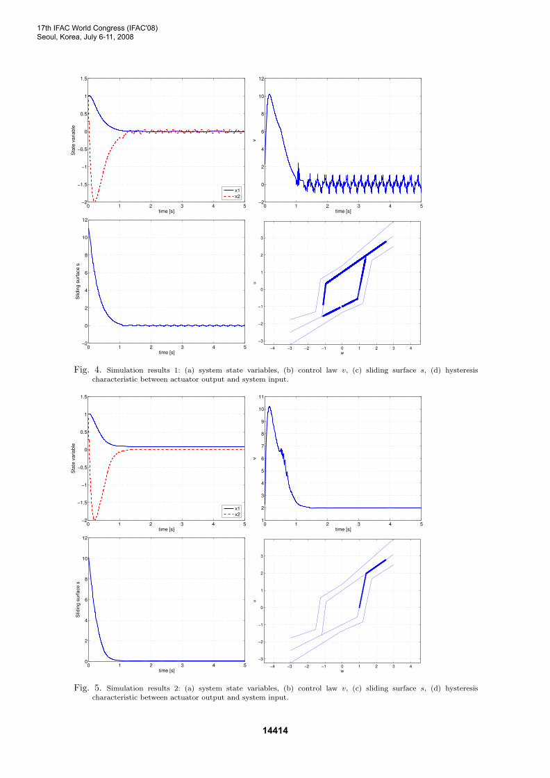
s(x) = λx1 + x2.Two simulation results have been included to show the ef-fectiveness of the proposed controller, addressing both thestabilization and the regulation problem of the mechanicalsystem. Note that no modifications have been found nec-essary for applying the main result to the regulation case,apart that of considering the error system instead of theplant itself.In both simulations initial conditions have been set x0 =[1 1]T , xA(0) = 0.5. λ parameter has been set λ = 10. Inthe regulation problem we chose the desired final positionequal to x1 = 5 degrees.It can be easily observed that control goals stated inproblem 2.1 have been achieved. Figures 4 and 5 (a) showthe time evolution of state variables x1 and x2 of the plantapproaching to zero or the desired position (x1 = 0.0873rad). Panels 4 and 5 (b) show the time evolution of thecontrol law v, in figures 4 and 5 (c) is reported timeevolution of sliding surfaces s which behave as expected.Finally panels 4 and 5 (d) display the points (marked) ofthe hysteresis characteristic used by the controller.

6. CONCLUSIONS

In this work the problem of stabilizing a system with sand-wiched nonsmooth nonlinearity with uncertain parameters

between two nonlinear uncertain SISO system has beenaddressed.This note has proposed an output feedback sliding modecontroller ensuring the convergence of the system trajecto-ries in a neighborhood of the origin for a sandwich systemwith hysteresis.Simulation results confirm the effectiveness of the pre-sented solution.

REFERENCES

M. L. Corradini, G. Orlando and G. Parlangeli. “AVSC Approach for the Robust Stabilization of Nonlin-ear Plants With Uncertain Nonsmooth Actuator Non-linearities - A Unified Framework”. IEEE Trans. onAutomatic Control, vol. 49, No. 5, May 2004, pp. 807-813.

M. L. Corradini, G. Orlando and G. Parlangeli. “RobustControl of Nonlinear Uncertain Systems with Sand-wiched Backlash”. In Proc. on 44th IEEE Conferenceon Decision and Control, and the European ControlConference 2005, Sevilla, Spain, December 12-15, 2005.

T.-L. Chern and J.-S. Wong. “DSP based integral variablestructure control for DC motor servo drivers”. IEEProc.-Control Theory Appl., vol. 142, No. 5., September1995, pp. 444-450.

H. K. Khalil. Nonlinear Systems, 3rd Edition. Prentice-Hall, 2002, pp. 610-625.

F. L. Lewis, K. Liu, R. Selmic and L.-X. Wang. ‘Adaptivefuzzy logic compensation of actuator deadzones”. J.Robot. Syst., vol. 14, 1997, pp. 501-511.

R. Marino and P. Tomei. “Global Adaptive Output-Feedback Control of Nonlinear Systems, Part I: LinearParameterization”. IEEE Trans. on Automatic Control,vol. 38, No. 1, January 1993, pp. 17-21.

J. J. Slotine and S. S. Sastry. “Tracking control of nonlin-ear systems using sliding surfaces, with application torobot manipulators”. in Int. J. Control, vol. 38, No. 2,1983, pp. 465-492.

G. Tao and P. V. Kokotovic. Adaptive Control of SystemsWith Actuator and Sensor Nonlinearities. New York:Wiley, 1996.

G. Tao, X. Ma and Y. Ling. “Optimal and nonlinear de-coupling control of system with sandwiched backlash”.Automatica, vol. 37, 2001, pp. 165-176.

A. Taware, G. Tao and C. Teolis. “Design and analysisof a hybrid control scheme for sandwich nonsmoothnonlinear systems”. IEEE Transactions on AutomaticControl, vol. 47, 2002, pp. 145-150.

A. Taware and G. Tao. “Analysis and control of sandwichsystems”. Proc. 38th IEEE Conference on Decision andControl, Phoenix, Arizona, USA, December 07-10, 1999,pp. 1156-1161.

V. I. Utkin. Sliding Modes in Control Optimization, NewYork: Springer-Verlang, 1992.

X. Zhao and Y. Tan. “Neural Adaptive Control of Dy-namic Sandwich Systems with Hysteresis”. Proceedingsof the 2006 IEEE International Symposium on Intelli-gent Control, Munich, Germany, October 04-06, 2006.

17th IFAC World Congress (IFAC'08)Seoul, Korea, July 6-11, 2008

14413

0 1 2 3 4 5−2

−1.5

−1

−0.5

0

0.5

1

1.5

time [s]

Sta

te v

aria

ble

x1

x2

0 1 2 3 4 5−2

0

2

4

6

8

10

12

time [s]

v

0 1 2 3 4 5−2

0

2

4

6

8

10

12

time [s]

Slid

ing

su

rfa

ce

s

−4 −3 −2 −1 0 1 2 3 4

−3

−2

−1

0

1

2

3

w

u

Fig. 4. Simulation results 1: (a) system state variables, (b) control law v, (c) sliding surface s, (d) hysteresischaracteristic between actuator output and system input.

0 1 2 3 4 5−2

−1.5

−1

−0.5

0

0.5

1

1.5

time [s]

Sta

te v

aria

ble

x1

x2

0 1 2 3 4 51

2

3

4

5

6

7

8

9

10

11

time [s]

v

0 1 2 3 4 50

2

4

6

8

10

12

time [s]

Slid

ing

su

rfa

ce

s

−4 −3 −2 −1 0 1 2 3 4

−3

−2

−1

0

1

2

3

w

u

Fig. 5. Simulation results 2: (a) system state variables, (b) control law v, (c) sliding surface s, (d) hysteresischaracteristic between actuator output and system input.

17th IFAC World Congress (IFAC'08)Seoul, Korea, July 6-11, 2008

14414