Robust optimization of adiabatic tapers for coupling to ...

Robust optimization of adiabatic tapersfor coupling to slow-light

photonic-crystal waveguides

Ardavan Oskooi,1,∗ Almir Mutapcic,2 Susumu Noda,1

J. D. Joannopoulos,3 Stephen P. Boyd,4 and Steven G. Johnson5

1Department of Electronic Science and Engineering, Kyoto University, Kyoto 615-8510, Japan2Sarajevo School of Science and Technology, Sarajevo 71000, Bosnia and Herzegovina

3Department of Physics, Massachusetts Institute of Technology, Cambridge MA 02139, USA4Department of Electrical Engineering, Stanford University, Stanford CA 94305, USA

5Department of Mathematics,Massachusetts Institute of Technology, Cambridge MA 02139, USA

∗[email protected]

Abstract: We investigate the design of taper structures for coupling toslow-light modes of various photonic-crystal waveguides while taking intoaccount parameter uncertainties inherent in practical fabrication. Our short-length (11 periods) robust tapers designed for λ = 1.55 μm and a slow-lightgroup velocity of c/34 have a total loss of < 20dB even in the presence ofnanometer-scale surface roughness, which outperform the correspondingnon-robust designs by an order of magnitude. We discover a posteriori thatthe robust designs have smooth profiles that can be parameterized by afew-term (intrinsically smooth) sine series which helps the optimization tofurther boost the performance slightly. We ground these numerical resultsin an analytical foundation by deriving the scaling relationships betweentaper length, taper smoothness, and group velocity with the help of an exactequivalence with Fourier analysis.

© 2012 Optical Society of America

OCIS codes: (050.1755) Computational electromagnetic methods; (130.0250) Optoelec-tronics; (130.5296) Photonic crystal waveguides; (250.5300) Photonic integrated circuits;(350.4238) Nanophotonics and photonic crystals.

References and links1. S. Cox and D. Dobson, “Maximizing band gaps in two-dimensional photonic crystals,” SIAM J. Appl. Math 59,

2108–2120 (1999).2. S. Cox and D. Dobson, “Band structure optimization of two-dimensional photonic crystals in H-polarization,” J.

Comp. Physics 158, 214–224 (2000).3. L. Frandsen, A. Harpoth, P. Borel, M. Kristensen, and J. Jensen, “Broadband photonic crystal waveguide 60◦

bend obtained utilizing topology optimization,” Opt. Express 12, 5916–5921 (2004).4. P. Borel, A. Harpoth, L. Frandsen, M. Kristensen, P. Shi, J. Jensen, and O. Sigmund, “Topology optimization and

fabrication of photonic crystal structures,” Opt. Express 12, 1996–2001 (2004).5. D. Dobson and F. Santosa, “Optimal localization of eigenfunctions in an inhomogeneous medium,” SIAM J.

Appl. Math 64, 762–774 (2004).6. W. Frei, D. Tortorelli, and H. Johnson, “Topology optimization of a photonic crystal waveguide termination to

maximize directional emission,” Appl. Phys. Letters 86(111114) (2005).7. A. Hakansson, J. Sanchez-Dehesa, and L. Sanchis, “Inverse design of photonic crystal devices,” IEEE J. Selected

Areas in Communications 23, 1365–1371 (2005).8. C. Kao, S. Osher, and E. Yablonovitch, “Maximizing band gaps in two-dimensional photonic crystals,” Appl.

Phys. B 81, 235–244 (2005).

#171622 - $15.00 USD Received 29 Jun 2012; revised 24 Aug 2012; accepted 25 Aug 2012; published 5 Sep 2012(C) 2012 OSA 10 September 2012 / Vol. 20, No. 19 / OPTICS EXPRESS 21558

9. N. Ikeda, Y. Sugimoto, Y. Watanabe, N. Ozaki, A. Mizutani, Y. Takata, J. Jensen, O. Sigmund, P. Borel, M. Kris-tensen, and K. Asakawa, “Topology optimised photonic crystal waveguide intersections with high-transmittanceand low crosstalk,” Elec. Letters 42, 1031–1033 (2006).

10. W. Frei, D. Tortorelli, and H. Johnson, “Geometry projection method for optimizing photonic nanostructures,”Opt. Letters 32, 77–79 (2007).

11. L. He, C.-Y. Kao, and S. Osher, “Incorporating topological derivatives into shape derivatives based level setmethods,” J. Comp. Physics 225, 891–909 (2007).

12. J. Riishede and O. Sigmund, “Inverse design of dispersion compensating optical fiber using topology optimiza-tion,” J. Opt. Soc. Am. B 25, 88–97 (2008).

13. O. Sigmund and K. Hougaard, “Geometric properties of optimal photonic crystals,” Phys. Rev. Letters100(153904) (2008).

14. D. Dobson and L. Simeonova, “Optimization of periodic composite structures for sub-wavelength focusing,”Appl. Math. Optim. 60, 133–150 (2009).

15. R. Matze, J. Jensen, and O. Sigmund, “Systematic design of slow-light photonic waveguides,” J. Opt. Soc. Am. B28, 2374–2382 (2011).

16. Y. Elesin, B. Lazarov, J. Jensen, and O. Sigmund, “Design of robust and efficient photonic switches using topol-ogy optimization,” Photon. and Nanostruc. 10, 153–165 (2012).

17. T. Happ, M. Kamp, and A. Forchel, “Photonic crystal tapers for ultracompact mode conversion,” Opt. Letters 26,1102–1104 (2001).

18. A. Mekis and J. Joannopoulos, “Tapered couplers for efficient interfacing between dielectric and photonic crystalwaveguides,” J. Lightwave Tech. 19(6), 861–865 (2001).

19. M. Palamaru and P. Lalanne, “Photonic crystal waveguides: out of plane losses and adiabatic modal conversion,”Appl. Phys. Letters 78, 1466–1468 (2001).

20. P. Sanchis, J. Marti, J. Blasco, A. Martinez, and A. Garcia, “Mode matching technique for highly efficient cou-pling between dielectric waveguides and planar photonic crystal circuits,” Opt. Express 10, 1391–1397 (2002).

21. A. Talneau, P. Lalanne, M. Agio, and C. Soukoulis, “Low-reflection photonic-crystal taper for efficient couplingbetween guide sections of arbitrary widths,” Opt. Letters 27, 1522–1524 (2002).

22. P. Bienstman, S. Assefa, S. Johnson, J. Joannopoulos, G. Petrich, and L. Kolodziejski, “Taper structures forcoupling into photonic crystal slab waveguides,” J. Opt. Soc. Am. B 20, 1817–1821 (2003).

23. N. Moll and G.-L. Bona, “Comparison of three-dimensional photonic crystal slab waveguides with two-dimensional photonic crystal waveguides: efficient butt coupling into these photonic crystal waveguides,” J. Appl.Physics 93, 4986–4991 (2003).

24. P. Sanchis, J. Garcia, A. Martinez, F. Cuesta, A. Griol, and J. Marti, “Analysis of adiabatic coupling between pho-tonic crystal single-line-defect and coupled-resonator optical waveguides,” Opt. Letters 28, 1903–1905 (2003).

25. E. Miyai and S. Noda, “Structural dependence of coupling between a two-dimensional photonic crystal waveg-uide and a wire waveguide,” J. Opt. Soc. Am. B 21, 67–72 (2004).

26. P. Sanchis, P. Bienstman, B. Luyssaert, R. Baets, and J. Marti, “Analysis of butt coupling in photonic crystals,”IEEE J. Quant. Elec. 40, 541–550 (2004).

27. E. Khoo, A. Liu, and J. Wu, “Nonuniform photonic crystal taper for high-efficiency mode coupling,” Opt. Express13, 7748–7759 (2005).

28. P. Sanchis, J. Marti, W. Bogaerts, P. Dumon, D. V. Thourhout, and R. Baets, “Experimental results on adia-batic coupling into SOI photonic crystal coupled-cavity waveguides,” IEEE Photon. Tech. Letters 17, 1199–1201(2005).

29. K. Dossou, L. Botten, C. de Sterke, R. McPhedran, A. Asatryan, S. Chen, and J. Brnovic, “Efficient couplers forphotonic crystal waveguides,” Opt. Commun. 265, 207–219 (2006).

30. Y. Vlasov and S. McNab, “Coupling into the slow light mode in slab-type photonic crystal waveguides,” Opt.Letters 31, 50–52 (2006).

31. J. Hugonin, P. Lalanne, T. White, and T. Krauss, “Coupling into slow-mode photonic crystal waveguides,” Opt.Letters 32, 2638–2640 (2007).

32. P. Pottier, M. Gnan, and R. D. L. Rue, “Efficient coupling into slow-light photonic crystal channel guides usingphotonic crystal tapers,” Opt. Express 15, 6569–6575 (2007).

33. C. de Sterke, J. Walker, K. Dossou, and L. Botten, “Efficient slow light coupling into photonic crystals,” Opt.Express 15, 10,984–10,990 (2007).

34. P. Velha, J. Hugonin, and P. Lalanne, “Compact and efficient injection of light into band-edge slow-modes,” Opt.Express 15, 6102–6112 (2007).

35. J. Lu, S. Boyd, and J. Vuckovic, “Inverse design of a three-dimensional nanophotonic resonator,” Opt. Express19, 10,563–10,570 (2011).

36. J. Lu and J. Vuckovic, “Objective-first design of high-efficiency, small-footprint couplers between arbitrarynanophotonic waveguide modes,” Opt. Express 20, 7221–7236 (2012).

37. M. Povinelli, S. Johnson, and J. Joannopoulos, “Slow-light, band-edge waveguides for tunable time delays,” Opt.Express 13(8), 7145–7159 (2005).

38. J. D. Joannopoulos, S. G. Johnson, R. D. Meade, and J. N. Winn, Photonic Crystals: Molding The Flow Of Light,


2nd ed. (Princeton Univ. Press, 2008).39. T. Baba, “Slow light in photonic crystals,” Nat. Photonics 2, 465–473 (2008).40. S. Johnson, P. Bienstman, M. Skorobogatiy, M. Ibanescu, E. Lidorikis, and J. Joannopoulos, “Adiabatic theorem

and continuous coupled-mode theory for efficient taper transitions in photonic crystals,” Phys. Rev. E 66(066608)(2002).

41. G. Taguchi, R. Jugulum, and S. Taguchi, Computer-Based Robust Engineering: Essentials For DFSS (ASQQuality Press, 2004).

42. A. Bental, L. E. Ghaoui, and A. Nemirovski, Robust Optimization (Princeton University Press, 2009).43. A. Mutapcic, S. Boyd, A. Farjadpour, S. Johnson, and Y. Avniel, “Robust design of slow-light tapers in periodic

waveguides,” Engineering Optimization 41, 365–384 (2009).44. D. Bertsimas, O. Nohedani, and K. Teo, “Robust optimization for unconstrained simulation-based problems,”

Oper. Research 58, 161–178 (2010).45. F. Wang, J. Jensen, and O. Sigmund, “Robust topology optimization of photonic crystal waveguides with tailored

dispersion properties,” J. Opt. Soc. Am. B 28, 387–397 (2011).46. P. Bienstman and R. Baets, “Optical modelling of photonic crystals and VCSELs using eigenmode expansion

and perfectly matched layers,” Opt. and Quant. Electronics 33, 327–341 (2001).47. T. White, L. Botten, C. de Sterke, K. Dossou, and R. McPhedran, “Efficient slow-light coupling in a photonic

crystal waveguide without transition region,” Opt. Letters 33, 2644–2646 (2008).48. A. Kurs, J. D. Joannopoulos, M. Soljacic, and S. G. Johnson, “Abrupt coupling between strongly dissimilar

waveguides with 100% transmission,” Opt. Express 19, 13,714–13,721 (2011).49. M. L. Povinelli, M. Ibanescu, S. G. Johnson, and J. D. Joannopoulos, “Slow-light enhancement of radiation

pressure in an omnidirectional-reflector waveguide,” Appl. Phys. Letters 85, 1466–1468 (2004).50. J. Ma and M. Povinelli, “Effect of periodicity on optical forces between a one-dimensional periodic photonic

crystal waveguide and an underlying substrate,” Appl. Phys. Letters 97(151102) (2010).51. A. Oskooi, P. Favuzzi, Y. Kawakami, and S. Noda, “Tailoring repulsive optical forces in nanophotonic waveg-

uides,” Opt. Letters 36, 4638–4640 (2011).52. Y. Xu, R. Lee, and A. Yariv, “Propagation and second-harmonic generation of electromagnetic waves in a

coupled-resonator optical waveguide,” JOSA-B 17(387–400) (2000).53. M. Soljacic, S. G. Johnson, S. Fan, M. Ibanescu, E. Ippen, and J. D. Joannopoulos, “Photonic-crystal slow-light

enhancement of non-linear phase sensitivity,” J. Opt. Soc. Am. B 19, 2052–2059 (2002).54. S. Anderson, A. Shroff, and P. Fauchet, “Slow light with photonic crystals for on-chip optical interconnects,”

Adv. Opt. Technology 2008(293531) (2008).55. J. Hastings, M. Lim, J. Goodberlet, and H. Smith, “Optical waveguides with apodized sidewall gratings via

spatial-phase- locked electron-beam lithography,” J. Vac. Sci. Tech. B 20, 2753–2757 (2002).56. T. Segawa, S. Matsuo, Y. Ohiso, T. Ishii, and H. Suzuki, “Apodised sampled grating using InGaAsP/InP deep-

ridge waveguide with vertical-groove surface grating,” Elec. Letters 40, 804–805 (2004).57. M. Strain and M. Sorel, “Design and fabrication of integrated chirped bragg gratings for on-chip dispersion

control,” IEEE J. Quant. Elec. 46, 774–782 (2010).58. G. Strang, Computational Science and Engineering (Welleseley-Cambridge Press, Wellesley MA, 2007).59. S. Boyd and L. Vandenberghe, Convex Optimization (Cambridge University Press, Cambridge, UK, 2004).60. M. Ghebrebrhan, P. Bermel, Y. Avniel, J. D. Joannopoulos, and S. G. Johnson, “Global optimization of silicon

photovoltaic cell front coatings,” Opt. Express 17, 7505–7518 (2009).61. P. Bermel, M. Ghebrebrhan, W. Chan, Y. X. Yeng, M. Araghchini, R. Hamam, C. H. Marton, K. F. Jensen,

M. Soljacic, J. D. Joannopoulos, S. G. Johnson, and I. Celanovic, “Design and global optimization of high-efficiency thermophotovoltaic systems,” Opt. Express 18, A314–A334 (2010).

62. S. Fan, P. R. Villeneuve, and J. D. Joannopoulos, “Theoretical investigation of fabrication-related disorder on theproperties of photonic crystals,” J. Appl. Physics 78, 1415–1418 (1995).

63. J. Foresi, P. Villeneuve, J. Ferrera, E. Thoen, G. Steinmeyer, S. Fan, J. Joannopoulos, L. Kimerling, H. Smith,and E. P. Ippen, “Photonic-bandgap microcavities in optical waveguides,” Nature 390, 143–145 (1997).

64. S. G. Johnson and J. D. Joannopoulos, “Block-iterative frequency-domain methods for Maxwell’s equations in aplanewave basis,” Opt. Express 8(3), 173–190 (2001).

65. J. E. Avron and A. Elgart, “Adiabatic theorem without a gap condition,” Commun. Math. Physics 203, 445–463(1999).

66. K. O. Mead and L. M. Delves, “On the convergence rate of generalized Fourier expansions,” IMA J. Appl. Math.12(3), 247–259 (1973).

67. J. P. Boyd, Chebyshev And Fourier Spectral Methods, 2nd ed. (Springer, 1989).68. A. Oskooi, L. Zhang, Y. Avniel, and S. Johnson, “The failure of perfectly matched layers, and towards their

redemption by adiabatic absorbers,” Opt. Express 16(15), 11,376–11,392 (2008).69. S. G. Johnson, M. L. Povinelli, P. Bienstman, M. Skorobogatiy, M. Soljacic, M. Ibanescu, E. Lidorikis, and

J. D. Joannopoulos, “Coupling, scattering and perturbation theory: semi-analytical analyses of photonic-crystalwaveguides,” in Proc. 2003 5th Intl. Conf. on Transparent Optical Networks and 2nd European Symp. on Pho-tonic Crystals, vol. 1, pp. 103–109 (2003).


70. P. Bienstman, “CAMFR: CAvity Modeling FRamework,” Software at http://camfr.sourceforge.net.71. M. L. Povinelli, S. G. Johnson, E. Lidorikis, J. D. Joannopoulos, and M. Soljacic, “Effect of a photonic band gap

on scattering from waveguide disorder,” Appl. Phys. Letters 84, 3639–3641 (2004).72. S. Assefa, P. T. Rakich, P. Bienstman, S. G. Johnson, G. S. Petrich, J. D. Joannopoulos, L. A. Kolodziejski, E. P.

Ippen, and H. I. Smith, “Guiding 1.5μm light in photonic crystals based on dielectric rods,” Appl. Phys. Letters85, 6110–6112 (2004).

73. A. Taflove and S. C. Hagness, Computational Electrodynamics: The Finite-Difference Time-Domain Method, 3rded. (Artech, Norwood, MA, 2005).

74. A. F. Oskooi, D. Roundy, M. Ibanescu, P. Bermel, J. D. Joannopoulos, and S. G. Johnson, “MEEP: A flexiblefree-software package for electromagnetic simulations by the FDTD method,” Comp. Phys. Communications181, 687–702 (2010).

75. J. Nocedal and S. Wright, Numerical Optimization (Springer, New York, 1999).76. A. Conn, N. Gould, and P. Toint, Trust Region Methods (SIAM, Philadelphia, PA, 2000).

1. Introduction

In this paper, we combine large-scale optimization, an increasingly popular tool in nanophoton-ics [1–16], with robustness and slow light for the problem of coupling two dissimilar waveg-uides [17–36]: here, a conventional dielectric waveguide and a periodic waveguide with a“slow-light” band edge [37–39] where the group velocity approaches zero. We start with thebasic idea of an “adiabatic taper,” a gradual transition that allows wide-bandwidth efficientcoupling [40], and apply optimization (∼ 1000 parameters) to design the best “profile” of thetaper rate for a given taper length L, in order to minimize the tradeoff between taper length Land taper reflectivity R. We obtain < 20dB reflection for L of only a few periods, but weshow that the problem becomes intrinsically more difficult as the group velocity decreases,and the resulting optimized designs become more and more counterintuitive. A key idea in ourapproach is the use of robust optimization [41–45]: optimization that takes into account manu-facturing uncertainty (e.g. fabrication disorder or errors in the dielectric constant or operatingfrequency) by always optimizing the worst-case perturbation to any design. Building on ourprevious work [43], we show that traditional “nominal” optimization (i.e., assuming no uncer-tainty) in photonic devices such as this one can easily lead to disaster: an optimized device thatperforms well only because of some delicate interference cancellation, and whose performanceadvantage is destroyed even by tiny manufacturing errors. In contrast, the robust optimum de-grades much more gracefully in the presence of errors: by taking into account the possibilityof errors from the beginning, the robust optimization procedure tends to avoid designs that relyon delicate cancellations. Rather than expensive simulations of the full Maxwell equations per-formed during the optimization procedure [18,20,21,25,34–36], rapid semi-analytical coupled-mode theory (CMT) [40] calculations are possible for the taper-design problem [37,43]—theseinitially perform small Maxwell simulations only for the periodic building blocks of the taperto determine the waveguide modes, and subsequently compute a simple integral (equivalent toa weighted Fourier transform) to find the reflectivity of any given taper profile. CMT trades offefficiency for generality, but is an indispensable tool to make large-scale optimization feasiblefor gradual tapers, especially in 3d. We find that, in the CMT context, the robustness helps us inanother way: by comparison to brute-force scattering-matrix calculations [46], we find that ourdesigns are also robust to computational approximations. Even with robustness, however, as thegroup velocity becomes lower we show that large-scale (many-parameter) optimization tendsto push towards an artificial solution that exaggerates discrepancies between the optimizationmodel and the physical circumstances (e.g. modelling errors and/or imperfect uncertainty mod-els), a tendency that can be combatted by building in a posteriori observations about the natureof the robust optima. In particular, we observe that the robust optima tend to be smooth, slowly-oscillating shapes that can be parameterized as a linear taper plus a truncated sine series with afew terms, and by using this information a priori, in addition to robust optimization, we obtain


parameter s = 0

parameter s = 1

z

going from uniform waveguide to periodic waveguide...

or

or

(e.g. s ~ hole radius, flange width, block spacing, ...)

s = 0

s = 1

L

s=0

s=1

z=0 z=L

design s(z/L)

...100s of parameters...

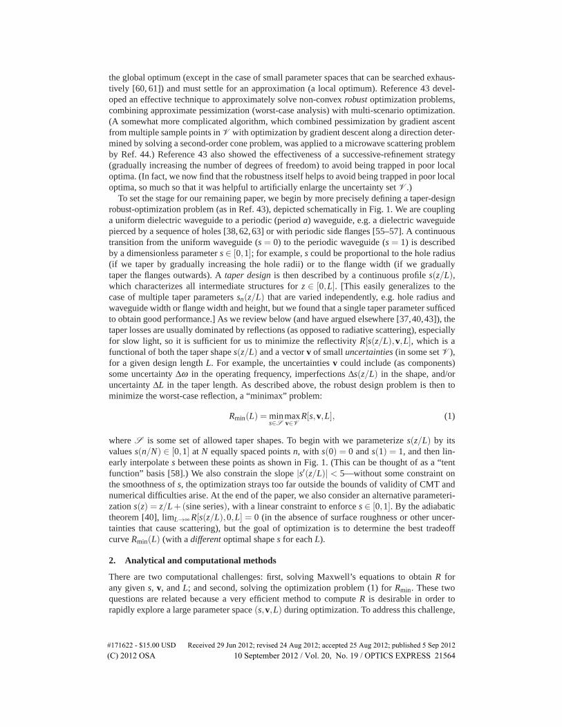
Fig. 1. Schematic taper design problem, with a transition between two waveguides charac-terized by a dimensionless parameter s ∈ [0,1]. The taper goes from a uniform dielectricwaveguide (s = 0) to a periodic waveguide (s = 1), with 0 < s < 1 describing intermediatestructures (e.g. s ∼ hole radius, flange width, or block spacing in the structures shown atright). A taper design (bottom) is a “shape” function s(z/L) (for z ∈ [0,L]) describing acontinuous transition from s(0) = 0 to s(1) = 1. For optimization, we parameterize s by itsvalues at uniformly spaced points and linearly interpolate in between (bottom left).

an improved design at very low group velocities. Although we show analytically that smooth-ness reduces taper reflections asymptotically for long tapers, the desirability of smoothness foroptimized short tapers is not as apparent, especially in light of many previous coupler designsemploying abrupt transitions [20, 23, 25, 26, 30, 33, 34, 47, 48].

The coupling of optical modes from one structure to another is crucial for enabling com-plex integrated photonic devices. A particular challenge is posed by slow-light waveguides,which are useful since their low group velocity enhances many types of light-matter in-teraction [39] as well as enhancing dispersion effects [37]. For example, the slow-light in-crease of the field intensity boosts the optical force in optomechanical systems [49–51],and it also enhances nonlinear effects for a variety of applications [39, 52–54]. Many de-signs have been proposed for coupling dissimilar waveguides (in most cases at moder-ate group velocities), including designs based on butt-coupling [23, 26], mode-field match-ing [20, 25, 30, 47], anti-reflection coatings [33, 34], resonant transmission [48], and gradualtaper transitions [17–19, 21, 22, 24, 27–29, 31, 32, 36, 37, 40, 43]. Most of these works involvedonly a small number of tunable degrees of freedom, which (combined with the moderate groupvelocities) helped to avoid the ultra-sensitive nonmanufacturable designs that tend to arise whenmany degrees of freedom are included; hence, they were able to disregard uncertainties during


the design process. Resonance can be used to couple to slow light, but is intrinsically narrow-band and relies on a delicate cancellation represented by a forced impedance matching (al-though, being a single parameter, manufacturing errors could conceivably be compensated bypost-fabrication tuning) [48]. Strong frequency and parameter sensitivity was also encounteredin the optimization of a coupler over many degrees of freedom [7]. To address a similar problemin our earlier work, we introduced one simple way of incorporating robustness by optimizingthe worst-case performance over a large (±30%) range of rescaled taper lengths for the sameshape [37]. In particular, we designed an adiabatic taper for coupling to a slow-light 3d flangedwaveguide (with a moderately low group velocity of c/10) having low reflection (< 20dB),and optimizing over shapes parameterized by a few parameters (degree-4 polynomials) [37].However, it is desirable to develop a framework in which more general uncertainties can beincorporated. To this end, we recently demonstrated a method for designing waveguide tapersthat takes into account uncertainties in the operating frequency and taper shape while using alarge number (hundreds) of free parameters [43]. As a proof of concept, we designed a fixed-length (30 periods) taper (to periodic 2d blocks) by smoothly varying the air gaps, coupling toa mode at a moderate group velocity of c/4 [43]. Here, we extend that work to a more realis-tic waveguide taper (a waveguide with periodic side flanges, which can be gradually extendedwhile avoiding arbitrarily narrow air gaps), closely analogous to the fabricatable [55–57] 3dflanged waveguide considered in Ref. 37, but in two dimensions so as to be amenable to brute-force validation of its performance in the face of fabrication imperfections (surface roughness).Furthermore, rather than looking at a fixed taper length as in our previous works, we inves-tigate the central engineering tradeoff in this problem: the tradeoff between performance andtaper length, by comparing separately-optimized structures at different lengths. We go downto a group velocity of c/34, where the taper problem becomes even more challenging (bothphysically and in the optimization sense, e.g. we find that low group velocity required morealgorithmic effort to avoid being trapped in poorly-performing local optima, and also requiresmore care to maintain the validity of CMT). Finally, we extend the asymptotic analysis of theadiabatic limit (taper length → ∞) from our previous works [37, 40] to address the interplaybetween taper smoothness, group velocity, and reflection (with the help of an exact equivalenceto Fourier analysis that we derive here).

In a sense, all engineering design is a problem of optimization: choosing some design pa-rameters p to optimize some objective O(p), possibly subject to some constraints. Large-scaleoptimization (sometimes called “inverse design”) is simply optimization in the regime wherethere are many parameters, so many that one cannot easily intuit the form of the solution. (Withmany parameters, it is crucial that one evaluate the gradient ∇pO analytically, which can be ef-ficiently achieved by an adjoint method [58].) There are many algorithms to solve optimizationproblems of many different kinds, but robust optimization is not about the choice of algorithm,it is about changing the optimization problem. Instead of solving a nominal optimization likeminp O(p), in which the optimization process assumes that O is known exactly with no uncer-tainties, robust optimization techniques transform the problem to incorporate uncertainties. Ifthe uncertainties are described as unknown values v in some set V (e.g. the error bars of man-ufacturing variability), then one way to “robustify” the problem is to optimize the worst case,minp[maxv O(p,v)]. (There are also other possibilities, such as optimizing the average case, butworst-case optimization benefits from the availability of many practical algorithms [43]. Refer-ence 45 employed a simplified worst-case analysis for a waveguide-design problem, in whichthe worst of three designs was optimized.) Most previous work on robust optimization focusedon “convex” optimization problems [59]—essentially, problems with no suboptimal local min-ima, which can therefore be efficiently solved exactly. However, design problems in optics,including the taper design problem here, are typically nonconvex: one cannot in general find


the global optimum (except in the case of small parameter spaces that can be searched exhaus-tively [60, 61]) and must settle for an approximation (a local optimum). Reference 43 devel-oped an effective technique to approximately solve non-convex robust optimization problems,combining approximate pessimization (worst-case analysis) with multi-scenario optimization.(A somewhat more complicated algorithm, which combined pessimization by gradient ascentfrom multiple sample points in V with optimization by gradient descent along a direction deter-mined by solving a second-order cone problem, was applied to a microwave scattering problemby Ref. 44.) Reference 43 also showed the effectiveness of a successive-refinement strategy(gradually increasing the number of degrees of freedom) to avoid being trapped in poor localoptima. (In fact, we now find that the robustness itself helps to avoid being trapped in poor localoptima, so much so that it was helpful to artificially enlarge the uncertainty set V .)

To set the stage for our remaining paper, we begin by more precisely defining a taper-designrobust-optimization problem (as in Ref. 43), depicted schematically in Fig. 1. We are couplinga uniform dielectric waveguide to a periodic (period a) waveguide, e.g. a dielectric waveguidepierced by a sequence of holes [38, 62, 63] or with periodic side flanges [55–57]. A continuoustransition from the uniform waveguide (s = 0) to the periodic waveguide (s = 1) is describedby a dimensionless parameter s ∈ [0,1]; for example, s could be proportional to the hole radius(if we taper by gradually increasing the hole radii) or to the flange width (if we graduallytaper the flanges outwards). A taper design is then described by a continuous profile s(z/L),which characterizes all intermediate structures for z ∈ [0,L]. [This easily generalizes to thecase of multiple taper parameters sn(z/L) that are varied independently, e.g. hole radius andwaveguide width or flange width and height, but we found that a single taper parameter sufficedto obtain good performance.] As we review below (and have argued elsewhere [37,40,43]), thetaper losses are usually dominated by reflections (as opposed to radiative scattering), especiallyfor slow light, so it is sufficient for us to minimize the reflectivity R[s(z/L),v,L], which is afunctional of both the taper shape s(z/L) and a vector v of small uncertainties (in some set V ),for a given design length L. For example, the uncertainties v could include (as components)some uncertainty Δω in the operating frequency, imperfections Δs(z/L) in the shape, and/oruncertainty ΔL in the taper length. As described above, the robust design problem is then tominimize the worst-case reflection, a “minimax” problem:

Rmin(L) = mins∈S

maxv∈V

R[s,v,L], (1)

where S is some set of allowed taper shapes. To begin with we parameterize s(z/L) by itsvalues s(n/N) ∈ [0,1] at N equally spaced points n, with s(0) = 0 and s(1) = 1, and then lin-early interpolate s between these points as shown in Fig. 1. (This can be thought of as a “tentfunction” basis [58].) We also constrain the slope |s′(z/L)| < 5—without some constraint onthe smoothness of s, the optimization strays too far outside the bounds of validity of CMT andnumerical difficulties arise. At the end of the paper, we also consider an alternative parameteri-zation s(z) = z/L+(sine series), with a linear constraint to enforce s ∈ [0,1]. By the adiabatictheorem [40], limL→∞ R[s(z/L),0,L] = 0 (in the absence of surface roughness or other uncer-tainties that cause scattering), but the goal of optimization is to determine the best tradeoffcurve Rmin(L) (with a different optimal shape s for each L).

2. Analytical and computational methods

There are two computational challenges: first, solving Maxwell’s equations to obtain R forany given s, v, and L; and second, solving the optimization problem (1) for Rmin. These twoquestions are related because a very efficient method to compute R is desirable in order torapidly explore a large parameter space (s,v,L) during optimization. To address this challenge,


we first review CMT and its application as a numerical method, and also discuss its analyticalimplications for the asymptotic properties of gradual tapers. We also compare CMT with more“brute-force” simulation algorithms, which are used both for validation of CMT and for post-optimization evaluation of our designs in the face of disorder. Finally, we briefly review theoptimization algorithm, which was developed in detail in our previous work [43].

2.1. Coupled-mode theory and the adiabatic limit

In order to compute R, as in our previous work [37, 43] we employ the coupled-mode the-ory (CMT) developed in Ref. 40. The basic idea is to expand the field in the waveguidein the basis of the Bloch eigenmodes of periodic waveguides—here, the waveguide modescorresponding to the intermediate structure s(z/L) is used to expand the fields at that z. Ab-stractly, if the electromagnetic field is ψ(z) (with xy coordinates omitted), we write ψ(z) =∑n cn(z)ψn(z)exp[i

∫ z βn(z′)dz′], where the ψn(z) are the Bloch eigenmodes at z, βn is the cor-responding propagation constant (or wavevector), and cn is the expansion coefficient. Whenthis expansion is substituted into the Maxwell equations, a set of coupled ODEs for cn(z) isobtained (the “coupled-mode” or “coupled-wave” equations) [40]. In the L → ∞ limit, the adi-abatic theorem states that the expansion coefficients are constants [cn(z)→ cn(0)], while for afinite L we can apply a slowly varying envelope approximation (SVEA) to compute the correc-tions to this limit. In the SVEA, assuming we start with a single incident mode cn(0) = δn0, tolowest order in the rate of change one finds that the reflected-wave amplitude cr is [40]:

cr =∫ 1

0dus′(u)∑

k

Mk[s(u)]Δβk[s(u)]

eiL∫ u0 Δβk[s(u

′)]du′ . (2)

Here, Mk(s) is a coupling matrix element (an overlap integral 〈ψi| · · · |ψr〉) of the incident andreflected fields with the geometric variation, and Δβk(s) = βr(s)−βi(s)+2πk/a(s) is a phase-mismatch factor between the incident (i) and reflected (r) modes summed over all Brillouinzones (all integers k). In this paper, the Mk and Δβk parameters were obtained from a planewave-expansion method [64]. In practice, the sum over k converges rapidly [40] so we only included|k| < 3. The reflected power is then R = |cr|2. Computation of the gradient ∇scr is describedin Ref. 43. (It is important to contrast this Bloch-mode expansion with older coupled-wave ap-proaches that expand in the basis of uniform waveguide modes of each cross-section, which isineffective as a semi-analytical technique for strongly periodic structures in which the cross sec-tion is rapidly varying [40]. A Bloch-mode basis, on the other hand, experiences no scatteringat all from the periodicity itself—it only undergoes intermodal scattering when the periodicityis broken by the taper, and is therefore a rapidly converging basis for gradual taper transitionsof periodic structures, including structures whose unit cells contain discontinuities such as airgaps [40].)

In principle, the total loss (1− transmission) includes radiative scattering in addition to re-flection (assuming single-mode waveguides so that there is no other inter-modal reflection).However, the reflected power tends to dominate [40], especially for slow-light modes (lowgroup velocity vg = dω/dβ ), as can be argued from (2) [37]. First, at a quadratic band edge ina periodic waveguide, Δβ ∼ vg (for the k term corresponding to modes β = π/a±Δ coupled inadjacent Brillouin zones)—this both decreases the denominator in (2) and decreases the phasemismatch. Second, the modes in coupled-mode theory are normalized to unit power [40], andhence the fields scale ∼ 1/

√vg and there is an additional 1/vg factor in M for coupling slow-

light incident and reflected modes, versus only a 1/√

vg factor in M for coupling slow-lightincident to non-slow scattered waves [37].

In order to understand the validity of CMT and the precise scaling with group velocity,we must have a better understanding of the adiabatic limit. A particularly elegant approach


is to make a change of variables to transform (2) into a Fourier integral, at which point all ofthe well-known properties of Fourier transforms can be invoked. Omit the k summation forsimplicity (e.g. focus on the dominant k term). The key point is that one generally (with rareexceptions [65]) considers adiabatic transitions in which the incident and scattered modes arenever degenerate in β , so that Δβ is always nonzero. This is certainly true for the case ofreflections. The function x(u) =

∫ u0 Δβk[s(u′)]du′ is therefore monotonic, and one can invert it

to u(x) and change variables u ↔ x. We obtain precisely a Fourier integral:

cr =∫ ∞

−∞dxs′(u(x))

Mk[s(u(x))]Δβk[s(u(x))]2

eiLx, (3)

where we are free to extend the integration range since s′ = 0 outside the taper. As long ass is continuous, so that s′ contains no delta functions, this → 0 for L → ∞ because L is sim-ply the “frequency” of a convergent Fourier transform. Furthermore, the rate at which cr → 0with L is well known in Fourier theory to depend on the smoothness of the integrand [66, 67],which in this case is determined by the smoothness of s′ (including the taper endpoints). Forexample, if s is a simple linear taper with discontinuous slope s′ at the taper ends, then theFourier transform (due to the discontinuity) scales as cr ∼ 1/L, hence the reflections go as 1/L2

asymptotically [37, 40]. More generally, if s has endpoint discontinuities in its �-th derivativeand is otherwise smooth, then |cr|2 ∼ 1/L2� [66, 67] (we previously analyzed a related point inthe context of PML absorbing boundaries, where the Fourier analogy was not so exact [68]).Similarly, the group-velocity scaling depends on the smoothness of s. For the case of a lineartaper, or any taper with discontinuous s′, the reflection goes as |cr|2 ∼ |M/Δβ |2/L2 ∼ 1/(Lv3

g)2,

or equivalently we must have L ∼ 1/v3g to obtain a fixed reflection [37,69]. For smoother tapers,

the convergence analysis of the Fourier integral involves integration by parts to apply additionalderivatives to s until the discontinuity is reached [66–68], which gives additional du/dx= 1/Δβfactors by the chain rule. Hence, the generalization to a discontinuity in the �-th derivative is a

scaling |cr|2 ∼ |M/Δβ |2/(LΔβ )2� ∼ (1/v4g)/(Lvg)

2�, or L ∼ 1/v1+2/�g . The consequence of this

scaling is that a tradeoff of taper length with group velocity becomes (asymptotically) betterfor smoother tapers, approaching L ∼ 1/vg, and so smoothness—eliminating high-frequencyFourier components—of the taper shape may be especially important for slow light. On theother hand, the optimum taper shape is very different for any given finite L than it is in theasymptotic limit—the rule is not simply “smoother is better,” because smoother tapers alsotend to require a larger L to attain the asymptotic 1/L2� behavior [68]. Optimization is requiredto determine the best shape for any finite L, especially for short L far from the asymptoticregime.

2.2. Brute-force numerics and validation

CMT, when evaluated to lowest-order as in (2), is asymptotically exact in the limit of gradualtapers, but is only an approximation for the rapid taper transitions that are the goal of opti-mization because we are neglecting multiple-scattering effects. (Note that our expansion basisis that of Bloch modes [40], so multiple-scattering effects of the periodicity itself are treatedexactly; it is only multiple scattering between Bloch modes due to the taper transition thatare neglected.) Fortunately, the optimization will also tend to drive the taper shape preciselyinto the small-|cr| regime where CMT is accurate. However, to check the performance of ourtaper designs, we supplement the CMT with a brute-force numerical calculation based on aneigenmode-expansion scattering-matrix method (also called RCWA, the rigorous coupled-waveapproximation) via the free CAMFR package [70]. CAMFR is also used as a final check of therobustness of the designs to fabrication errors, since in that method we can incorporate random


surface roughness in the taper (which requires a different coupled-mode theory technique to de-scribe it accurately [71]). In general, we found that the robust-optimization approach produceddesigns that were robust even in the face of errors in the computational method, whereas weshow below that nominal optimization produces designs whose performance is destroyed evenby slight changes in the simulation accuracy.

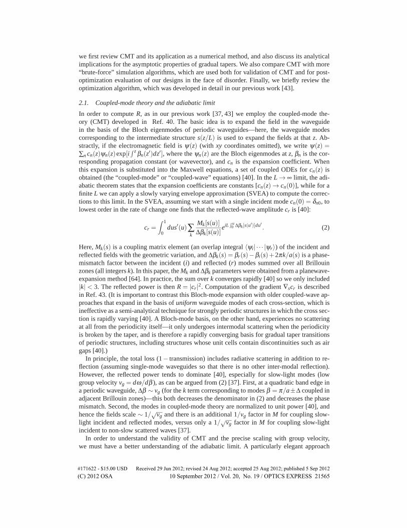
Figure 2(a) shows a linear (forward and backward, double) taper between a uniform waveg-uide and a sequence of dielectric blocks (ε = 12), for relatively “fast” light (vg ≈ c/4) in theTM (out-of-plane E) polarization, with excellent agreement between CAMFR and CMT exceptfor very short tapers with reflections > 10%. This structure is convenient for validation [40,43]because its piecewise-constant cross-sections are particularly efficient in CAMFR and allowus to study very long and gradual tapers, but it is relatively difficult to realize experimentallybecause its tapers involve many extremely narrow air gaps (that must be abruptly merged inpractice once the limits of lithographic resolution are reached [72]). In Fig. 2(b), we insteadconsider a (TE-polarized) case of a waveguide with lateral flanges [55–57] operating close tothe band edge where the group velocity is ≈ c/34. This sort of geometry is experimentallyattractive because a gradual taper involves no arbitrarily narrow features, and the TE polariza-tion translates into a TE-like polarization in three dimensions that can be confined by muchthinner structures than TM-like polarizations [38]. In this case, however the CMT only beginsto converge to the CAMFR results (which we also check against a third numerical method,FDTD [73, 74]) for very long tapers, but this is not unexpected. Because of the slow light usedhere, the reflections are very large (∼ 40%), and the first-order approximation in our CMT isexpected to be inaccurate. For slow light, as explained above, a simple linear taper is a poorchoice even if the taper can be made quite long: although CMT predicts an asymptotic 1/L2

scaling of the reflection, we would need to go to much larger lengths to observe this scaling forslow light. [Unfortunately, CAMFR is far more expensive for the taper in (b) than for the taperin (a), due to the nonconstant cross-sections in the former, while FDTD is also too expensive tosimulate a very gradual taper.] As we show below, however, optimizing the CMT in the slow-light case nevertheless yields a (much more counterintuitive) design that performs well even inthe brute-force CAMFR check.

2.3. Robust-optimization algorithm

The basic optimization algorithm, as described in Ref. 43, is sequential linear programming(SLP) with a trust-region constraint [75, 76]. In order to implement the robustness [the innermaxv of (1)], the method uses the gradient ∇vR to estimate the worst-case v parameters for thecurrent shape s (and in fact accumulates a memory of ten such worst cases over the course ofthe optimization that it uses for subsequent steps), and thus transforms the continuous maxvinto a discrete “multi-scenario” maximization over a finite set of worst-case candidates [43].

Reference 43 also introduced a technique of “successive refinement”: we gradually increasethe number of degrees of freedom (from 1 to 1024, roughly doubling in each step), using theoptimized coarser structures as starting points for optimization of the finer structures. This pro-cedure has two benefits: it both increases the robustness of the design (by making it more robustto coarsening the discretization of s) and also tends to avoid becoming immediately trapped inlocal minima (although we cannot guarantee that the final result is a global minimum).

We found that the precise details of the set V of uncertainties makes relatively littledifference—putting in any robustness tends to force the optimization to avoid delicate can-cellations that would be sensitive to any errors. However, some care is required in the case ofslow light because of the presence of a band edge beyond which the guided mode no longerexists. As the band edge is approached, any uncertainty Δω in the operating frequency mustbe reduced to avoid going past this band edge. In practice, if a fabrication error were to shift


refl

ectio

n fr

om

doub

le ta

per

design taper length (periods)a)

10- 3

10- 2

10- 1

100

10 20 30 40 50 60 70 80 90 100

scatteringmatrix

coupled-mode theory

vg=c/4

b)

Fig. 2. Comparison of coupled-mode theory (CMT) calculation of reflection coefficientfrom double taper (from uniform to periodic to uniform) structure, using a simple lin-ear profile s(u) = u, with two other brute-force numerical methods, scattering matrix(CAMFR [46]) and finite-difference time-domain (FDTD [74]). (a) 2d period a 0.4a×0.4ablocks example (top left) with TM operating mode at vg = c/4 [40,43]. CMT and CAMFRagree well. (b) 2d period-a flanged waveguide (inner width a, outer width 2a, 50% dutycycle) with TE operating mode at vg = c/34, adapted from Ref. 37 (top right). For suchslow light, the scattering from a short linear taper is too large for CMT to be valid, but op-timization of the taper shape will drive the reflections low enough for the CMT calculationto be suitable.

the band edge slightly, an application requiring slow light would have to either adjust the op-erating frequency accordingly or perform post-fabrication tuning (e.g. by thermally changingthe refractive index) in order to keep vg fixed. Therefore, to reflect this situation of fixed vg,we did not include any uncertainty in ω . However, in order to represent the possibility of er-ror in the phase velocity (ω/β ) that could result from such post-fabrication tuning, we insteadincluded an uncertainty ΔL in the taper length L [equivalent to an overall shift in β by (2)].Since ∂β/∂ω diverges as vg → 0, we increased the uncertainty in L (and hence in β ) as we de-creased vg—failing to do this resulted in designs that were overly sensitive to fabrication errorsin our simulations. Furthermore, we found that decreasing vg made the optimization increas-ingly susceptible to being trapped in poor local minima—intuitively, the increased reflections inthe slow-light regime also increase the number of opportunities for delicate cancellations—andincreasing ΔL helped to combat this tendency. We also included random perturbations in s (ateach discretized s point), but we found that this made little difference in the resulting designonce ΔL was sufficiently large.

3. Results

We now discuss the results of optimizing and simulating taper designs for the two differentwaveguides of Fig. 2, considering both slow light and moderate group velocities, for both nom-inal (mins R) and robust (mins maxv R optimization), with and without introducing “fabricationdisorder” (surface roughness) in the simulation (after optimizing).

3.1. Periodic blocks

To begin with, we return to the periodic (period a) sequence of 0.4a× 0.4a blocks (dielectricconstant ε = 12 in air) from Fig. 2(a) that we studied in Ref. 43, operating at the same moderate


a) b)

c) d)position, u=z/L

tape

r pro

file

, s(u

)

0.50 10

0.5

1

nominal

robust

linearnominal

0.04 0.08 0.12

0.04

0.08

0.12

L=50a

10- 8

10- 6

10- 4

10- 2

100

100design taper length (periods)

refl

ectio

n fr

om d

oubl

e ta

per

0 10 20 30 40 50 60 70 80 90

scattering matrix

coupled-mode theory

nominal (no disorder)

10- 8

10- 6

10- 4

10- 2

100

0 10 20 30 40 50 60 70 80 90 100

linearnominal

robust

design taper length (periods)

refl

ectio

n fr

om d

oubl

e ta

per

scattering matrix (no disorder)

10- 10

10- 8

10- 6

10- 4

10- 2

100

rescaled taper length (periods)

refl

ectio

n fr

om d

oubl

e ta

per

0 10 20 30 40 50 60 70 80 90 100

linear

nominal

robust

coupled-mode theory

50 100010-7

10-1

10-4 cmt

sm

Fig. 3. Optimization results for taper structure of square blocks (operating TM mode withvg = c/4) from Fig. 2(a), with block spacing as the taper variable (top: linear tapers). (a)Performance of three tapers (linear in green, nominal optimum in blue, and robust optimumin red, with the optimizations performed independently at each length L) computed usinga brute-force scattering-matrix method (CAMFR [46]) (with no disorder introduced). (b)Performance of nominal taper (optimized independently at each taper length) computed us-ing two different methods (CMT and CAMFR)—the large disparity is due to the nominaloptimum relying on a delicate interference cancellation that is destroyed even by the slightnumerical differences between the two techniques. (c) Performance of linear, nominal, androbust tapers designed at L = 50a and then rescaled to other taper lengths: the nominaloptimum relies on a delicate cancellation that only works close to L = 50a. Inset comparesCMT and CAMFR for the L = 20a design rescaled to different lengths, and illustrates thatthe two approaches agree everywhere except at L = 20a, where there is a delicate interfer-ence cancellation that is inherently irreproducible (non-robust), and at small L where thereflection exceeds 10% (causing CMT to break down). (d) Nominal and robust taper pro-files s(u) designed at L = 50a: the nominal design is only slightly different from a lineartaper, with the slight changes (inset) sufficient to create a delicate reflection cancellation.


group velocity of c/4 and coupled to a uniform waveguide of width 0.4a, which is a convenienttest problem because of the ease of comparison with brute-force CAMFR simulation. Unlikeour previous work, however, we now perform the optimization of s separately for every taperlength L ∈ [1,100]a, in order to examine the tradeoff of optimal Rmin with L. We then simulateeach of the resulting taper designs in CAMFR in order to verify their performance.

The results are shown in Fig. 3(a), and exhibit a surprising phenomenon: even when nodisorder (no roughness) is introduced into the scattering-matrix (CAMFR) calculation, so thatin principle it should be modeling exactly the same system as the CMT calculations used duringoptimization, the nominal optimum exhibits worse performance than the robust optimum (andboth are better than a simple linear taper). Mathematically, one would expect that the nominaloptimum should always perform at least as well as the robust optimum when the disorder is setto zero, simply because maxv R[s,v]≥ R[s,0]. The reason for the behavior in Fig. 3(a) is simple,however: the nominal optimum relies on such a delicate cancellation effect that even the slightdifference in simulation accuracy between CAMFR and CMT (both will have simulation errors,but the errors will be different) is sufficient to radically degrade the performance of the nominaloptimum, while the robust optimum still performs well. As shown below, when the nominaland robust optima are evaluated in CMT, the nominal performance is indeed slightly better.

This discretization-error degradation in the nominal optimum can be seen in Fig. 3(b), whichcompares the CMT and CAMFR calculations for the nominal optimum at each L. For very shorttapers, they make comparable predictions, but once the taper is about 10a in length the opti-mization is able to engineer a delicate cancellation that causes the CMT reflections to suddenlydrop by four orders of magnitude (at which point they become limited by numerical errorsand cease to improve further). Even the slight difference in discretization error induced by theswitch from CMT to CAMFR, however, is enough to destroy this cancellation. (In our previouswork, we showed for this structure that the robust optimum remained an order of magnitudebetter than the nominal optimum even after additional disorder is intentionally introduced intothe CAMFR calculation [43]; we consider such disorder in the next section.) The agreement ofCMT and CAMFR everywhere except at the point of this delicate cancellation is demonstratedbelow, using the inset of Fig. 3(c).

Another viewpoint on this delicate cancellation is shown in Fig. 3(c), which considers thedesign s for L = 50a, but then plots the performance of the same taper shape s(z/L) when itis rescaled to other lengths L. The nominal optimum performs well only at the design lengthof L = 50a, and its performance immediately degrades to little better than a linear taper shape(s(u) = u) as soon as it is rescaled to a different L—this is a signature of a delicate destructivecancellation in the reflected wave that the nominal optimization forced to occur at L = 50a.The inset compares CMT and CAMFR for a rescaled L = 20a design, and shows that thetwo agree except at L = 20a where the non-robust cancellation occurs, which is destroyed byslight differences in discretization error as discussed above. In contrast, the robust optimum stillperforms well even when s is rescaled to lengths L very different from the L where the shape wasdesigned—the robust optimum does not rely on a delicate cancellation that is easily destroyed.(As expected, the nominal optimum at L= 50a is indeed slightly better than the robust optimumat that L, when the two are evaluated in CMT with no disorder.) The corresponding taper shapess are shown in Fig. 3(d): while the robust optimum is a relatively smooth transition that flattensat the ends (reducing the s′ discontinuities of a linear taper as might be expected from theasymptotic analysis), the nominal optimum is nearly identical to a linear taper, only deviatingby a slight amount (inset) that is apparently tuned to force a reflection cancellation at L = 50a.

Finally, we should comment on one other interesting feature of Fig. 3(a): for the robustoptimum, the reflections appear to decrease exponentially with L until reaching a “noise floor”around 10−6 imposed by numerical accuracy limitations. An exponential tradeoff of reflection


a)

0

0.5

1 nominal

0.50 10

0.5

1 robust

position, u=z/L

tape

r pro

file

, s(u

)

"fine"

b)

Fig. 4. Optimization results for taper from uniform to flanged waveguide (operating TEmode with vg = c/6) from Fig. 2(b), with flange (outer) width as the taper variable (top:linear tapers). (a) Performance of three tapers (linear in green, nominal optimum in blue,and robust optimum in red, with the optimizations performed independently at each lengthL) computed using a brute-force scattering-matrix method (CAMFR [46]), where surfaceroughness (±10−3a every 0.01a) was introduced, averaged over 50 structures. The robustoptimum maintains good (∼ 30 dB) performance even in the presence of disorder, whereasthe nominal optimum is greatly degraded. (b) Nominal and robust taper profiles designedat L = 13a (vertical axis exaggerated for clarity): the nominal design includes fine cusps(circled) absent from the robust design, whose apparent function is to introduce reflectioncancellations (which are spoiled by disorder).

with length is the ideal situation that would be attained asymptotically for an analytic tapershape (such as s(u) = tanh(u)/2+ 1/2), due to the exponential convergence of the Fouriertransforms of such analytic functions [67, 68], but this requires the taper to have an infinitelylong “tail”, and in any case only applies asymptotically for large L. In contrast, optimizationseems to attain a similar ideal tradeoff even for small L, even for finite-length tapers, albeit bychanging the taper shape as a function of L. (Whereas the linear and nominal tapers show 1/L2

scaling.)

3.2. Periodic flanges

Next, we consider taper designs to couple to a waveguide with period-a dielectric (ε = 12)flanges in air, as in Fig. 2(b): the flanges occupy 50% of each period, and extend to an outerdiameter (flange width) of 2a from an inner diameter of a (matching the uniform waveguide).Again, we optimize separately at each L, in this case for L ∈ [11,20]a (shorter than in theprevious section, both for computational tractability in brute force verification and also becauseshort tapers are more practical).

To start with, in Fig. 4, we operate at a moderate group velocity c/6, at a frequency ≈ 1%below the band edge of the fundamental mode. After optimization, we then simulated the result-ing structures in CAMFR, but modified to include disorder: uniform random surface roughnesswith amplitude ∈ [−10−3,10−3]a (corresponding to ≈ nm-scale surface roughness for opera-tion at λ = 1.55 μm) added to each slice (“pixel”) of thickness 0.01a of the taper. Each resultin Fig. 4(a) is the reflection averaged over 50 realizations of surface roughness. The robust op-timum is more than an order of magnitude better in performance than the nominal optimum—


again, the nominal optimum is better in the CMT but relies on delicate cancellations that aredestroyed by the surface roughness, although the nominal optimum is still slightly better thana simple linear taper. The robust design has reflections of ≈ 30 dB for a taper only L = 11ain length. The reflection improves for longer lengths, but only slowly, and eventually starts tobecome worse—the reason is that there is a tradeoff introduced by the surface roughness, inthat longer tapers are more gradual but also accumulate roughness-induced reflections over alonger length, and eventually the latter effect dominates. The nominal and robust designs forL = 13a are shown in Fig. 4(b); note that the vertical axis is exaggerated for clarity. The robusts(z/L) is a fairly smooth taper transition, exhibits some oscillatory behavior that seems hardto guess a priori (and s will become even more counter-intuitive when the group velocity isdecreased below). The nominal optimum is even more strange, with some fine cusps appearingin the first few taper flanges that almost certainly create reflections, albeit in such a way as toexactly cancel other reflections (e.g. from the taper ends) in the absence of disorder.

Next, we move to a more challenging problem: coupling to the same structure, but at afrequency only 0.01% below the band edge of the fundamental mode, operating at a group ve-locity of c/34. In this case, a simple linear taper exhibits > 30% reflections for a taper lengthL = 20a. In Fig. 5(a), we show the CAMFR simulations of the optimized designs at each L,again modifying the structures to include surface roughness. The robust optimum here exhibitsreflections < 20 dB, more than an order of magnitude better than the nominal optimum design,which is again only slightly better than a naive linear taper. The robust optimum, in fact, hasa dip < 40 dB in its reflections at L ∈ [13,15]a, apparently due to some destructive cancella-tion, but the dip disappears in Fig. 5(b) if we examine the total loss (1− transmission) insteadof just the reflections (which still dominate the loss for most L). Note that the losses againcan be seen to increase with L, an effect of the increased scattering from roughness along alonger length. In order to obtain the good performance for the robust taper, we found that weneeded to increase the amount of uncertainty ΔL in the optimization process to a relatively largevalue (3a), apparently to avoid being trapped in local minima. In fact, the nominal optimizationseemed to immediately become trapped in a relatively poor solution, even for the CMT withno uncertainty—as shown in Fig. 5(c), the nominal optimum achieves > 20 dB reflections inthe CMT, a performance that is destroyed when switching to CAMFR even with no surfaceroughness (due to discretization effects alone).

The nominal and robust optimum shapes s(u) for c/34 are shown in the lower-left and top-middle panels of Fig. 6 (again with the vertical axis enlarged for clarity). The nominal optimumhas even stronger cusps than in the c/6 velocity case, suggesting even more reliance on cancel-lations of strong interior reflections. However, even the robust optimum is highly oscillatory,with oscillations even within a single flange. Despite its good performance in the simulationsof Fig. 5, this led us to wonder whether the oscillatory shape was somehow an artifact of thechoice of parameterization of s. That is, is this merely a local minimum that we were trapped inas a consequence of discretizing s into piecewise linear (non-smooth) segments (tent functions)and gradually refining? To investigate this question, we repeated the robust optimization withan entirely different parameterization: s(u) = u+(sine series), where the sine series enforcesthe s(0) = 0 and s(1) = 1 boundary conditions. (The 0 ≤ s ≤ 1 boundary conditions were im-posed explicitly at 1000 points in u, which takes the form of a simple linear constraint added tothe linear-programming steps.) Successive refinement was performed by repeatedly doublingthe number of terms in the sine series (4,16,32,64), setting the new terms to zero as the startingpoint for optimization. The resulting robust sine-series optima are shown in Fig. 6 (lower-right),and are clearly converging towards the same oscillatory robust optimum. The 64-term sine se-ries s(u) is superimposed on the original robust optimum in the top-middle panel, and can beseen to reproduce even many of the fine features within each flange.


Fig. 5. Optimization results for taper from uniform to flanged slow-light waveguide (op-erating TE mode with vg = c/34) with flange (outer) width as the taper variable (top:linear tapers). (a) Performance of three tapers (linear in green, nominal in blue, and ro-bust in red, with the optimizations performed independently at each length) computedusing a brute-force scattering-matrix method (CAMFR [46]), where surface roughness(±10−3a every 0.01a) was introduced, averaged over 50 structures. (b) Same as (a) butwith 1− transmission: the inclusion of radiative scattering loss eliminates the optimization-created dip (cancellation) in the reflection losses from (a). As in Fig. 4, the robust optimumgreatly outperforms the nominal optimum in the presence of disorder. (c) Even withoutdisorder, the nominal optimum performs poorly in CAMFR compared to CMT: the slightdifferences in simulation accuracy are enough to spoil the nominal optimum. (d) Sameas (a) but with robust optimization using the original (1024-point) piecewise-linear (“tentfunction”) parameterization (red squares) compared to robust optimization using a sine-series parameterization (cyan) with 4, 16, and 64 terms: the latter is converging towardssimilar performance as the former, and towards similar structures as seen in Fig. 6, so therobust optimum is not merely a local minimum obtained as a byproduct of the discretizationchoice.


0

0.5

1

linearrobust (tent,1024)

robust (sine,64) robust (sine,64)

0.50 10

0.5

1

nominal

position, u=z/L0.50 1

robust (sine,16)

0.50 1

robust (sine,4)

tape

r pro

file

, s(u

)

a) b) c)

d) e) f)

Fig. 6. Linear, nominal, and robust-optimum taper profiles from the slow-light (c/34) op-timization of Fig. 5, optimized at a taper length L = 13a. Vertical axes are exaggerated forscale; topmost (black) figure shows the robust taper design to scale. Even the robust designshows complicated sub-flange oscillations, but similar oscillations are reproduced indepen-dent of the parameterization of the taper design during optimization. Top middle (red):robust design using 1024-point linear interpolation (tent functions). Cyan (bottom/right):robust optimization using sine series with successive increase of the number of series terms.64-term sine series structure (top right) is similar to tent-function (top middle) structure,and is superimposed on the latter as a dotted cyan curve. Nominal optimum (lower left) haseven more radical oscillations, designed to create delicate reflection cancellations (whichare spoiled by disorder).

The performance of these sine-series designs, shown in Fig. 5(d), is also converging towardsthe original robust optimum. In fact, the sine series for some L performs better with only 4 termsthan it does with more terms or with the original tent-function results. It may be, therefore, thatthe most counter-intuitive feature of the (tent or 64-sine) robust designs, the intra-flange oscil-lations, are an artifact not of the parameterization but of the model. That is, the optimizationis driving the design towards a regime in which the accuracy limitations of CMT and/or theuncertainty model (which cannot accurately capture surface roughness in the context of CMT)are being exploited to reduce reflections in a way that is partially spoiled in practice (e.g. inbrute-force calculations or in experiments). Although the robust designs still perform well, andit would not have been feasible to perform optimization of long tapers on a more exact model,these accuracy limitations can be further compensated for by building in a priori knowledgeof the solution: here, the observation that robust solutions tend to be smooth and slowly oscil-latory. (In hindsight, a few-term sine-series basis would have been sufficient to parameterizethe robust designs in Fig. 3 and Fig. 4 as well.) Robustness is still required: we have checkedthat nominal optimization applied to the sine-series parameterization continues to yield signifi-cantly worse results. In fact, for the L = 11a 4-term sine-series case where the robust optimum


performed very well, the nominal optimization is immediately trapped in a local minimum andits reflections stay above 10%.

4. Concluding remarks

We have demonstrated how a rapid, semi-analytical Maxwell solver combined with large-scale robust optimization can be used to design taper structures for slow-light photonic-crystalwaveguides with performance markedly better than their non-robust counterparts (nominal op-tima) in the presence of manufacturing variability. In three dimensions, our semi-analyticalCMT approach remains feasible [37], and currently seems to be the only feasible computa-tional method in 3d for optimizing the gradual tapers required in slow-light applications. Wehave shown that robustness, in addition to compensating for manufacturing uncertainty, canalso compensate for limitations of CMT to obtain designs that perform well in practice, eventhough CMT requires increasingly gradual tapers to be accurate as the group velocity decreases.Because we also find that the robust optima tend to be smooth, slowly-oscillating shapes, bybuilding this information into the parameterization a priori—parameterizing the shape as atruncated sine series with a few terms—we find that even better results can sometimes be ob-tained (although robust optimization is still important). (This finding is reminiscent of—butdoes not follow from—our analytical result that smooth shapes, with minimal high-frequencyFourier components of s′, reduce reflections in the asymptotic L → ∞ limit.) As the group ve-locity becomes lower, building in smoothness seems to become more and more important forrobustness. Using such an a priori low-dimensional representation has other potential bene-fits: combined with the efficiency of CMT it opens the possibility of more expensive globaloptimization approaches. Furthermore, these techniques are easily generalized to taper opti-mization for other waveguide designs, including in 3d, and other uncertainty models. As robusttaper designs are particularly useful for coupling to slow-light modes in realistic experimen-tal settings, they may potentially form a crucial component of complex, reconfigurable anddynamic optomechanical devices.

Acknowledgments

This work was supported in part by the AFOSR MURI for Complex and Robust On-chipNanophotonics under contract FA9550-09-1-0704 and by the U.S. Army Research Office un-der contract W911NF-07-D-0004. We are grateful to Professor Bjorn Maes at the University ofMons for assistance with CAMFR. A. Oskooi was supported by a postdoctoral fellowship fromthe Japan Society for the Promotion of Science (JSPS).


Robust optimization of adiabatic tapers for coupling to ...

Documents

Transcript of Robust optimization of adiabatic tapers for coupling to ...