Robust control system design by mapping specifications ...Robust Control System Design by Mapping...
143
Robust Control System Design by Mapping Specifications into Parameter Spaces Vom Promotionsausschuss der Fakult¨ at f¨ ur Elektrotechnik und Informationstechnik der Ruhr-Universit¨ at Bochum zur Erlangung des akademischen Grades Doktor-Ingenieur genehmigte DISSERTATION von Michael Ludwig Muhler aus Creglingen Bochum, 2007
-
Upload
duongxuyen -
Category
Documents
-
view
215 -
download
0
Transcript of Robust control system design by mapping specifications ...Robust Control System Design by Mapping...

Robust Control System Design
by Mapping Specifications
into Parameter Spaces
Vom Promotionsausschuss
der
Fakultat fur Elektrotechnik und Informationstechnik
der
Ruhr-Universitat Bochum
zur
Erlangung des akademischen Grades
Doktor-Ingenieur
genehmigte
D I S S E R T A T I O N
von
Michael Ludwig Muhler
aus Creglingen
Bochum, 2007


iii
Dissertation eingereicht am: 20. Oktober 2006
Tag der mundlichen Prufung: 20. Marz 2007
1. Berichter: Prof. Dr.-Ing. Jan Lunze
2. Berichter: Prof. Dr.-Ing. Jurgen Ackermann

iv
Fur meine Eltern, Ute und Maria

v
Acknowledgments
I am indebted to those who have given me the opportunity, support, and time to write
this doctoral thesis.
It is a pleasure to thank my advisor Professor Jurgen Ackermann for his encouragement
and advice during my studies. He has always been ready to give his time generously to
discuss ideas and approaches, while giving me the freedom to choose the direction of my
work. His insights and enthusiasm will have a long-lasting effect on me.
I would also like to thank my supervisor Professor Jan Lunze at the Ruhr-University
Bochum for his interest in my work. His support and willingness to work with me across
the miles and the years is greatly appreciated.
I am greatly indebted to my former office-mate, Paul Blue, for creating a friendly and
stimulating work atmosphere, and for many discussions, and also to my other colleagues
at DLR Oberpfaffenhofen, especially, Dr. Tilman Bunte, Dr. Dirk Odenthal, Dr. Dieter
Kaesbauer, Dr. Naim Bajcinca and Gertjan Looye.
Special thanks to Professor Bob Barmish, who initially encouraged me to pursue post-
graduate studies.
I would like to express my gratitude to Airbus for financial support during a three year
grant. Thanks to Dr. Michael Kordt, my contact at Airbus in Hamburg. Financial aid
from the DAAD for the conference presentations of parts of this thesis is gratefully ac-
knowledged.
The final write-up of this thesis would not have been possible without the support of my
supervisor at Robert Bosch GmbH, Dr. Hans-Martin Streib.
Finally, special thanks to my parents and to my wife Ute for their continuous encourage-
ment, patience and support.
Korntal-Munchingen, March 2007 Michael Muhler

vi

vii
Contents
Nomenclature xi
Abstract xiii
Zusammenfassung xiv
1 Introduction 1
1.1 The Control Problem . . . . . . . . . . . . . . . . . . . . . . . . . . . . . . 1
1.2 Background and Previous Research . . . . . . . . . . . . . . . . . . . . . . 2
1.3 Goal of the Thesis . . . . . . . . . . . . . . . . . . . . . . . . . . . . . . . 4
1.4 Outline . . . . . . . . . . . . . . . . . . . . . . . . . . . . . . . . . . . . . . 5
2 Control Specifications and Uncertainty 6
2.1 Parametric MIMO Systems . . . . . . . . . . . . . . . . . . . . . . . . . . 6
2.1.1 MIMO Specifications . . . . . . . . . . . . . . . . . . . . . . . . . . 8
2.1.2 MIMO Properties . . . . . . . . . . . . . . . . . . . . . . . . . . . . 8
2.2 Symbolic State-Space Descriptions . . . . . . . . . . . . . . . . . . . . . . 9
2.2.1 Transfer Function to State-Space Algorithm . . . . . . . . . . . . . 10
2.2.2 Minimal Realization . . . . . . . . . . . . . . . . . . . . . . . . . . 12
2.2.3 Example . . . . . . . . . . . . . . . . . . . . . . . . . . . . . . . . . 13
2.3 Uncertainty Structures . . . . . . . . . . . . . . . . . . . . . . . . . . . . . 14
2.3.1 Real Parametric Uncertainties . . . . . . . . . . . . . . . . . . . . . 16
2.3.2 Multi-Model Descriptions . . . . . . . . . . . . . . . . . . . . . . . 19
2.3.3 Dynamic Uncertainty . . . . . . . . . . . . . . . . . . . . . . . . . . 20
2.4 MIMO Specifications in Control Theory . . . . . . . . . . . . . . . . . . . 22
2.4.1 H∞ Norm . . . . . . . . . . . . . . . . . . . . . . . . . . . . . . . . 22
2.4.2 Passivity and Dissipativity . . . . . . . . . . . . . . . . . . . . . . . 26
2.4.3 Connections between H∞ Norm and Passivity . . . . . . . . . . . . 29
2.4.4 Popov and Circle Criterion . . . . . . . . . . . . . . . . . . . . . . . 30
2.4.5 Complex Structured Stability Radius . . . . . . . . . . . . . . . . . 33
2.4.6 H2 Norm Performance . . . . . . . . . . . . . . . . . . . . . . . . . 34

viii
2.4.7 Generalized H2 Norm . . . . . . . . . . . . . . . . . . . . . . . . . . 35
2.4.8 LQR Specifications . . . . . . . . . . . . . . . . . . . . . . . . . . . 36
2.4.9 Hankel Norm . . . . . . . . . . . . . . . . . . . . . . . . . . . . . . 38
2.5 Integral Quadratic Constraints . . . . . . . . . . . . . . . . . . . . . . . . . 38
2.5.1 IQCs and Other Specifications . . . . . . . . . . . . . . . . . . . . . 40
2.5.2 Mixed Uncertainties . . . . . . . . . . . . . . . . . . . . . . . . . . 41
2.5.3 Multiple IQCs . . . . . . . . . . . . . . . . . . . . . . . . . . . . . . 41
3 Mapping Equations 42
3.1 Eigenvalue Mapping Equations . . . . . . . . . . . . . . . . . . . . . . . . 42
3.2 Algebraic Riccati Equations . . . . . . . . . . . . . . . . . . . . . . . . . . 44
3.2.1 Continuous and Analytic Dependence . . . . . . . . . . . . . . . . . 46
3.3 Mapping Specifications into Parameter Space . . . . . . . . . . . . . . . . . 48
3.3.1 ARE Based Mapping . . . . . . . . . . . . . . . . . . . . . . . . . . 48
3.3.2 H∞ Norm Mapping Equations . . . . . . . . . . . . . . . . . . . . . 51
3.3.3 Passivity Mapping Equations . . . . . . . . . . . . . . . . . . . . . 53
3.3.4 Lyapunov Based Mapping . . . . . . . . . . . . . . . . . . . . . . . 54
3.3.5 Maximal Eigenvalue Based Mapping . . . . . . . . . . . . . . . . . 56
3.4 IQC Parameter Space Mapping . . . . . . . . . . . . . . . . . . . . . . . . 56
3.4.1 Uncertain Parameter Systems . . . . . . . . . . . . . . . . . . . . . 57
3.4.2 Kalman-Yakubovich-Popov Lemma . . . . . . . . . . . . . . . . . . 57
3.4.3 IQC Mapping Equations . . . . . . . . . . . . . . . . . . . . . . . . 59
3.4.4 Frequency-Dependent Multipliers . . . . . . . . . . . . . . . . . . . 60
3.4.5 LMI Optimization . . . . . . . . . . . . . . . . . . . . . . . . . . . 63
3.5 Complexity . . . . . . . . . . . . . . . . . . . . . . . . . . . . . . . . . . . 67
3.5.1 ARE Mapping Equations . . . . . . . . . . . . . . . . . . . . . . . . 67
3.5.2 Lyapunov Mapping Equations . . . . . . . . . . . . . . . . . . . . . 68
3.5.3 IQC Mapping Equations . . . . . . . . . . . . . . . . . . . . . . . . 69
3.6 Further Specifications . . . . . . . . . . . . . . . . . . . . . . . . . . . . . . 69
3.7 Comparison and Alternative Derivations . . . . . . . . . . . . . . . . . . . 70
3.8 Direct Performance Evaluation . . . . . . . . . . . . . . . . . . . . . . . . . 70
3.9 Summary . . . . . . . . . . . . . . . . . . . . . . . . . . . . . . . . . . . . 72
4 Algorithms and Visualization 73
4.1 Aspects of Symbolic Computations . . . . . . . . . . . . . . . . . . . . . . 74
4.2 Algebraic Curves . . . . . . . . . . . . . . . . . . . . . . . . . . . . . . . . 75
4.2.1 Asymptotes of Curves . . . . . . . . . . . . . . . . . . . . . . . . . 77
4.2.2 Parametrization of Curves . . . . . . . . . . . . . . . . . . . . . . . 77
4.2.3 Topology of Real Algebraic Curves . . . . . . . . . . . . . . . . . . 78
4.3 Algorithm for Plane Algebraic Curves . . . . . . . . . . . . . . . . . . . . . 80

ix
4.3.1 Extended Topological Graph . . . . . . . . . . . . . . . . . . . . . . 81
4.3.2 Bezier Approximation . . . . . . . . . . . . . . . . . . . . . . . . . 82
4.4 Path Following . . . . . . . . . . . . . . . . . . . . . . . . . . . . . . . . . 83
4.4.1 Common Problems of Path Following . . . . . . . . . . . . . . . . . 84
4.4.2 Homotopy Based Algorithm . . . . . . . . . . . . . . . . . . . . . . 84
4.4.3 Predictor-Corrector Continuation . . . . . . . . . . . . . . . . . . . 86
4.5 Surface Intersections . . . . . . . . . . . . . . . . . . . . . . . . . . . . . . 87
4.6 Preprocessing . . . . . . . . . . . . . . . . . . . . . . . . . . . . . . . . . . 88
4.6.1 Factorization . . . . . . . . . . . . . . . . . . . . . . . . . . . . . . 89
4.6.2 Scaling . . . . . . . . . . . . . . . . . . . . . . . . . . . . . . . . . . 89
4.6.3 Symmetry . . . . . . . . . . . . . . . . . . . . . . . . . . . . . . . . 89
4.7 Visualization . . . . . . . . . . . . . . . . . . . . . . . . . . . . . . . . . . 90
4.7.1 Color Coding . . . . . . . . . . . . . . . . . . . . . . . . . . . . . . 90
4.7.2 Visualization for Multiple Representatives . . . . . . . . . . . . . . 91
5 Examples 93
5.1 MIMO Design Using SISO Methods . . . . . . . . . . . . . . . . . . . . . . 93
5.2 MIMO Specifications . . . . . . . . . . . . . . . . . . . . . . . . . . . . . . 94
5.2.1 H2 Norm . . . . . . . . . . . . . . . . . . . . . . . . . . . . . . . . 94
5.2.2 H∞ Norm: Robust Stability . . . . . . . . . . . . . . . . . . . . . . 98
5.2.3 Passivity Examples . . . . . . . . . . . . . . . . . . . . . . . . . . . 100
5.3 Example: Track-Guided Bus . . . . . . . . . . . . . . . . . . . . . . . . . . 103
5.3.1 Design Specifications . . . . . . . . . . . . . . . . . . . . . . . . . . 104
5.3.2 Robust Design for Extreme Operating Conditions . . . . . . . . . . 105
5.3.3 Robustness Analysis . . . . . . . . . . . . . . . . . . . . . . . . . . 105
5.4 IQC Examples . . . . . . . . . . . . . . . . . . . . . . . . . . . . . . . . . . 106
5.5 Four Tank MIMO Example . . . . . . . . . . . . . . . . . . . . . . . . . . 110
6 Summary and Outlook 113
6.1 Summary . . . . . . . . . . . . . . . . . . . . . . . . . . . . . . . . . . . . 113
6.2 Outlook . . . . . . . . . . . . . . . . . . . . . . . . . . . . . . . . . . . . . 114
A Mathematics 115
A.1 Algebra . . . . . . . . . . . . . . . . . . . . . . . . . . . . . . . . . . . . . 115
A.2 Algebraic Riccati Equations . . . . . . . . . . . . . . . . . . . . . . . . . . 116
References 121

x

xi
Nomenclature
Acronyms
ARE algebraic Riccati equation, . . . . . . . . . . . . . . . . . . . . . . . . . . . . . . . . . . . . . . . . . p. 22
CRB complex root boundary, . . . . . . . . . . . . . . . . . . . . . . . . . . . . . . . . . . . . . . . . . . . . p. 44
IQC integral quadratic constraint, . . . . . . . . . . . . . . . . . . . . . . . . . . . . . . . . . . . . . . . p. 5
IRB infinite root boundary, . . . . . . . . . . . . . . . . . . . . . . . . . . . . . . . . . . . . . . . . . . . . . p. 44
KYP Kalman-Yakubovich-Popov, . . . . . . . . . . . . . . . . . . . . . . . . . . . . . . . . . . . . . . . . p. 57
LFR linear fractional representation, . . . . . . . . . . . . . . . . . . . . . . . . . . . . . . . . . . . . . p. 10
LHP left half plane, . . . . . . . . . . . . . . . . . . . . . . . . . . . . . . . . . . . . . . . . . . . . . . . . . . . . . . p. 43
LMI linear matrix inequality, . . . . . . . . . . . . . . . . . . . . . . . . . . . . . . . . . . . . . . . . . . . . p. 28
LQG linear quadratic Gaussian, . . . . . . . . . . . . . . . . . . . . . . . . . . . . . . . . . . . . . . . . . . p. 36
LQR linear quadratic regulator, . . . . . . . . . . . . . . . . . . . . . . . . . . . . . . . . . . . . . . . . . . p. 36
LTI linear time-invariant, . . . . . . . . . . . . . . . . . . . . . . . . . . . . . . . . . . . . . . . . . . . . . . . p. 6
MFD matrix fraction description, . . . . . . . . . . . . . . . . . . . . . . . . . . . . . . . . . . . . . . . . . p. 10
MIMO multi-input multi-output, . . . . . . . . . . . . . . . . . . . . . . . . . . . . . . . . . . . . . . . . . . . p. 6
PSA parameter space approach, . . . . . . . . . . . . . . . . . . . . . . . . . . . . . . . . . . . . . . . . . p. 2
RHP right half plane, . . . . . . . . . . . . . . . . . . . . . . . . . . . . . . . . . . . . . . . . . . . . . . . . . . . . p. 8
RRB real root boundary, . . . . . . . . . . . . . . . . . . . . . . . . . . . . . . . . . . . . . . . . . . . . . . . . . p. 44
SISO single-input single-output, . . . . . . . . . . . . . . . . . . . . . . . . . . . . . . . . . . . . . . . . . . p. 8

xii
Symbols
∗ conjugate transpose A(s)∗ = A(−s)T , . . . . . . . . . . . . . . . . . . . . . . . . . . . . . . . p. 24
ζ damping factor, . . . . . . . . . . . . . . . . . . . . . . . . . . . . . . . . . . . . . . . . . . . . . . . . . . . . p. 43
∼= equivalent state-space realization, . . . . . . . . . . . . . . . . . . . . . . . . . . . . . . . . . . . p. 7
:= definition, . . . . . . . . . . . . . . . . . . . . . . . . . . . . . . . . . . . . . . . . . . . . . . . . . . . . . . . . . . p. 22
den denominator, . . . . . . . . . . . . . . . . . . . . . . . . . . . . . . . . . . . . . . . . . . . . . . . . . . . . . . . p. 10
diag diagonal matrix, . . . . . . . . . . . . . . . . . . . . . . . . . . . . . . . . . . . . . . . . . . . . . . . . . . . . p. 11
Im image or range space of a matrix, . . . . . . . . . . . . . . . . . . . . . . . . . . . . . . . . . p. 117
Im imaginary part of imaginary number, . . . . . . . . . . . . . . . . . . . . . . . . . . . . . . . p. 43
⊗ Kronecker product, . . . . . . . . . . . . . . . . . . . . . . . . . . . . . . . . . . . . . . . . . . . . . . . . p. 115
⊕ Kronecker sum, . . . . . . . . . . . . . . . . . . . . . . . . . . . . . . . . . . . . . . . . . . . . . . . . . . . . p. 54
vec column stacking operator, . . . . . . . . . . . . . . . . . . . . . . . . . . . . . . . . . . . . . . . . . . p. 54
lcm least common multiple, . . . . . . . . . . . . . . . . . . . . . . . . . . . . . . . . . . . . . . . . . . . . . p. 10
Lm2 [0,∞) space of square summable functions, . . . . . . . . . . . . . . . . . . . . . . . . . . . . . . . . p. 39
Re real part of imaginary number, . . . . . . . . . . . . . . . . . . . . . . . . . . . . . . . . . . . . . p. 24
σ largest singular value, . . . . . . . . . . . . . . . . . . . . . . . . . . . . . . . . . . . . . . . . . . . . . . p. 22
σ singular value, . . . . . . . . . . . . . . . . . . . . . . . . . . . . . . . . . . . . . . . . . . . . . . . . . . . . . . p. 22
Λ eigenvalue spectrum, . . . . . . . . . . . . . . . . . . . . . . . . . . . . . . . . . . . . . . . . . . . . . . . p. 33
trace trace of a matrix, . . . . . . . . . . . . . . . . . . . . . . . . . . . . . . . . . . . . . . . . . . . . . . . . . . . p. 34
Variables
G(s) general transfer matrix, . . . . . . . . . . . . . . . . . . . . . . . . . . . . . . . . . . . . . . . . . . . . p. 7
q uncertain parameters, . . . . . . . . . . . . . . . . . . . . . . . . . . . . . . . . . . . . . . . . . . . . . . p. 3

xiii
Abstract
Robust controller design explicitly considers plant uncertainties to determine the con-
troller structure and parameters. Thereby, the given specifications for the control system
are fulfilled even under perturbations and disturbances.
The parameter space approach is an established methodology for systems with uncertain
physical parameters. Control specifications, for example formulated as eigenvalue criteria,
are hereby mapped into a parameter space. The graphical presentation of admissible
parameter regions leads to easily interpretable results and allows intuitive parametrization
and analysis of robust controllers.
The goal of this thesis is to extend the parameter space approach by new specifications
and to broaden the applicable system class. A uniform concept for mapping specifications
into parameter spaces is presented for this purpose. This enables the generalized deriva-
tion of mapping equations and the identical software implementation for the mapping.
Moreover, it allows to extend the parameter space approach by additional specifications
which can be mapped. Furthermore, the applicable system class can be broadened. All
relevant specifications for linear multivariable systems including the H2 and H∞ norm are
covered by this approach. Beyond that, specifications for nonlinear systems can be used
in conjunction with the parameter space approach. In particular, the mapping of integral
quadratic constraints is introduced.
A brief outline of specifications for multivariable systems introduces into the parameter
space mapping. All specifications are established using a similar mathematical description
that forms the basis for the generalized mapping equations. The mapping equations are
then obtained by converting the generalized algebraic specification description into a
specialized eigenvalue problem.
A symbolic-numerical algorithm is developed to realize the specification mapping. Various
graphical means to visualize the results in a parameter plane are explored. This is moti-
vated by specifications which yield a performance index. Various examples demonstrate
the extension of the parameter space approach and the new possibilities of the concept.

xiv
Zusammenfassung
Beim Entwurf von robusten Reglern werden Unsicherheiten der Regelstrecke explizit
berucksichtigt, um die Struktur und Parametrierung des Reglers so festzulegen, daß die
gestellten Anforderungen an das regelungstechnische System trotz auftretender Storungen
und Streckenveranderungen erfullt werden. Hierzu steht mit dem Parameterraumver-
fahren eine anerkannte Methodik fur Systeme mit unsicheren physikalischen Parame-
tern zur Verfugung. Hierbei werden regelungstechnische Spezifikationen, die zum Beispiel
als Eigenwertkriterien formuliert sind, in einen Parameterraum abgebildet. Die grafische
Darstellung von zulassigen Gebieten in einer Parameterebene fuhrt zu einfach interpretier-
baren Resultaten und ermoglicht die intuitive Parametrierung und Analyse von robusten
Reglern.
Ziel der Arbeit ist die Erweiterung des Parameterraumverfahrens um Spezifikationen sowie
die Vergroßerung der anwendbaren Systemklasse. Hierzu wird ein einheitliches Konzept
zur Abbildung von Spezifikationen in Parameterraume vorgestellt. Dieses erlaubt die ve-
rallgemeinerte Herleitung von Abbildungsgleichungen und die identische softwaretech-
nische Realisierung der Abbildung. Neben allen relevanten Spezifikationen fur lineare
Mehrgroßensysteme, wie die H2 und H∞ Norm, erlaubt das vorgestellte Konzept die
Anwendung des Parameterraumverfahrens auf nichtlineare Systeme. Insbesondere wird
die Abbildung von integral-quadratischen Bedingungen aufgezeigt.
Ein kurzer Abriß der Spezifikationen fur Mehrgroßensysteme fuhrt in die Abbildung in den
Parameterraum ein. Alle Spezifikationen werden in einer gleichartigen mathematischen
Formulierung dargestellt, die die Basis fur die verallgemeinerten Abbildungsgleichungen
bildet. Die Abbildungsgleichungen beruhen auf der Uberfuhrung der allgemeinen alge-
braischen Darstellung fur die Spezifikationen in ein spezielles Eigenwertproblem.
Um die Anwendung des hier vorgestellten Konzeptes zu ermoglichen, wird ein symbolisch-
numerischer Algorithmus zur Durchfuhrung der Abbildung von Spezifikationen entwick-
elt. Verschiedene Moglichkeiten zur grafischen Darstellung der Resultate in einer Pa-
rameterebene werden vorgestellt, insbesondere fur Spezifikationen die Gutewerte liefern.
Mehrere Beispiele stellen die Erweiterung des Parameterraumverfahrens und die neuen
Moglichkeiten des Konzeptes dar.

1
1 Introduction
1.1 The Control Problem
Why should we use feedback at all? The pure dynamics of a stable plant can be simply
modified to the desired dynamics using feedforward control.
In the real world every plant is subject to external disturbances. If we want to alter the
systems response to disturbances or signal uncertainty we have to use feedback.
Another fundamental reason for feedback control arises from instability. An unstable
plant cannot be stabilized by any feedforward system. Feedback control is mandatory for
these plants, even without signal and model uncertainty.
The third fundamental reason for using feedback control is the just mentioned model un-
certainty. The term model uncertainty here includes discrepancy between the true system
and the model used to design the controller. Reasons for deviations are model imperfec-
tions. For example, the modeling of an electric wire as a resistor is known to be perfect up
to a certain frequency range. More elaborate models derived from first principles might
include a resistor-capacitor chain. But even this model is only valid in a certain frequency
range because eventually the encountered physical phenomena reach atomic scale. Thus
model uncertainty is not just present in models obtained from measurements and iden-
tification. Every model, even a model derived from physical modeling, is only valid to a
certain extent.
Further model uncertainties can be design imposed, such as limitations on the complexity
of the design model or certain model types, for example linear models.
Classical control aims at stabilizing a system in the presence of signal uncertainty. Ro-
bust control extends this goal by designing control systems that not only tolerate model
uncertainties, but also retain system performance under plant variations.
While the goal that a feedback control system should maintain overall system performance
despite changes in the plant has been around since the early days of control theory, this
property is nowadays explicitly called robustness.

2 Introduction
1.2 Background and Previous Research
As a reaction to the poor robustness of controllers based on optimization and estimation
theory the field of robust control theory emerged, where plant variations play a key role.
Several different approaches to deal with plant variations mainly influenced by the uncer-
tainty characterization have evolved [Ackermann 1980, Doyle 1982, Lunze 1988, Safonov
1982]. Central topics in robust control theory common to all approaches are
• Uncertainty characterization.
• Robustness analysis.
• Robust controller synthesis.
For systems with real parametric uncertainty, e.g., an unknown or varying system param-
eter, the parameter space approach (PSA)1 is a well established method for robustness
analysis and robust controller design [Ackermann et al. 2002]. The basic idea of the pa-
rameter space approach is to map a condition of specification for a system into a plane of
parameters, i.e., the set of all parameters for which the specification holds is determined.
Initially the PSA considered eigenvalue specifications for linear systems. Its roots can be
traced back to the 19th century, where mathematicians such as [Hermite 1856, Maxwell
1866, Routh 1877], inspired by the first mechanical control systems, studied the basic
question related to stability of whether a given polynomial
p(s) = ansn + . . . + a1s + a0 = 0, (1.1)
has only roots with negative real parts. Interestingly these early accounts of stability ana-
lysis tried to find a solution that can be expressed using the coefficients of the polynomial,
thereby avoiding the explicit computation of roots.
Vishnegradsky was the first to visualize the stability condition in a coefficient parameter
plane in [1876], analyzing the stability of a third order polynomial p(s) = s3+a2s2+a1s+1
with respect to varying a1 and a2. This idea became the building block of the parameter
space approach.
Based on Hermite’s work, [Hurwitz 1895] reported an algebraic condition in terms of
determinants. This stability condition has been extensively used in control theory and
extended to robustness analysis.
Initially the parameter space method considered stability of a linear system described by
the characteristic equation. By mapping the stability condition it originally allowed to
analyze robustness with respect to two specific coefficients.
1Sometimes also referred to as parameter plane method

1.2 Background and Previous Research 3
The parameter space method was then extended to robust root clustering or Γ-stability,
by specifying an eigenvalue region [Ackermann et al. 1991, Mitrovic 1958]. This allows to
indirectly incorporate time-domain specifications and thereby robust performance.
The coefficients ai of (1.1) do not directly relate to plant or controller parameters, and
therefore hamper the application to control problems. Therefore robust control theory
considered polynomials with coefficients that depend on a parameter vector q ∈ Rp:
p(s, q) = an(q)sn + . . . + a1(q)s + a0(q) = 0. (1.2)
If q consists of only one parameter q, then robust stability can be evaluated by plotting
a generalized root locus [Evans 1948], where q takes the role of the usual linear gain k.
Robust, multimodal eigenvalue based parameter space approach is state-of-the-art. The
underlying theory is thoroughly understood for linear time-invariant systems with uncer-
tain parameters.
In general, the parameter space approach maps a given specification, e.g. a permissible
eigenvalue region, into a space of uncertain parameters q ∈ Rp, see Figure 1.1. Usually
the specification is mapped into a parameter plane because this leads to understandable
and powerful graphical results. Moreover, since we can map several specifications con-
secutively, this approach actually allows multiobjective analysis and synthesis of control
systems.
Recently, this approach was extended to the frequency domain for Bode specifications
[Besson and Shenton 1997, Hara et al. 1991, Odenthal and Blue 2000] and Nyquist dia-
grams [Bunte 2000]. Static nonlinearities were considered in the parameter space approach
in [Ackermann and Bunte 1999]. Finally [Muhler 2002] derived mapping equations for
multi-input multi-output systems, including H2,H∞ norms and passivity specifications.
During the 1990s there has been considerable interest in design methods such as H∞
and µ-analysis that require only control specifications and yield a controller including
the structure and parameters. While this seems to be attractive from the point that the
design engineer has not to waste time on thinking of a reasonable control structure and
possibly try several different structures. All of these design methods have the disadvantage
that they lead to very high controller orders. The direct order reduction of the resulting
controllers is a nontrivial task, and often destroys some of the required or desired features
of the initial high-order controllers.
Using the parameter space approach as a design tool we have to specify a controller
structure, e.g., a PID controller, and the parameters of the controller are iteratively tuned
until all design specifications are fulfilled. Thus the parameter space approach falls into
the category of fixed control structure design methods. Other approaches are given by
classical design methods or parameter optimization [Joos et al. 1999].

4 Introduction
σ q1
jω q2
p(s, q)
Figure 1.1: Mapping stability condition into parameter plane
The clear advantage of fixed structure methods is that the control engineer has full control
about the resulting complexity of the control system. This allows to handle implementa-
tion issues directly during the design process.
We will not consider special feedback structures in this thesis. This approach is backed
by the fact that all two degree of freedom configurations have basically the same prop-
erties and potentials, although some structures are especially suitable for some design
algorithms.
1.3 Goal of the Thesis
The main objective of this thesis is to extend the parameter space approach by new
specifications and to broaden the applicable system class, e.g., multivariable or nonlinear.
The basic idea of the parameter space approach (PSA) is to map control specifications
for a given system into the space of defined varying parameters. The boundaries of
parameter sets that fulfill the specifications are hereto determined. Usually we consider
two parameters at a time and control specifications are mapped into a parameter plane.
This allows intuitive interpretation of the graphical results.
By mapping we actually mean the identification of parameter regions (or subspaces) for
which the specifications are fulfilled. In other words we are interested in the set of all
parameters Pgood that fulfill a given specification. The boundary of this good set is
characterized by the equality case of the specification. Mathematically this good set is
given by a mapping equation.
Mapping equations form the mathematical core of the PSA. They combine the control
specific system description with specifications that a control design requires to hold for
the system.

1.4 Outline 5
This thesis presents a unified approach to consider various control specifications for multi-
variable systems in the parameter space approach. It is shown how various specifications
can be formulated using the same mathematical framework.
Since there is no straightforward way to solve the resulting mapping equations a second,
but not less important goal is to find and explore computational methods to solve the
mapping problem.
The results in this thesis can be transferred and applied to time-discrete systems. The
required methodology can be directly taken from [Ackermann et al. 2002]. Hence we do
not extensively cover the application of the time-continuous results in this thesis to the
time-discrete case.
1.4 Outline
Chapter 2 serves multiple purposes. We start with some control theoretic background.
Subsequently the various specifications are presented. Besides the introduction and some
information, the focus lies on a uniform mathematical description of the criteria. This
allows uniform treatment and development of mapping equations and finally mapping
algorithms.
Chapter 3 then presents the mapping equations used to map the specifications into pa-
rameter space. Beyond the mapping equations for specific specifications introduced in
Section 2.4, we consider mapping equations for general integral quadratic constraint (IQC)
specifications [Muhler and Ackermann 2004].
The remaining part of the thesis deals with the practical application of the presented con-
trol theory to practical problems. To this end, we take a closer look at algorithms suitable
for the mapping equations arising from the various control specifications in Chapter 4.
And we explore graphical means to visualize the results in a parameter plane. This is mo-
tivated by specifications that can be related to performance. Here not just the fulfillment
of a condition, for example stability, is crucial, but we are interested in optimizing the
attainable performance level. Therefore contour-like plots with color-coded performance
levels in a parameter plane reveal additional insight.
The application of the derived mapping equations and the mapping algorithms is demon-
strated on various examples in Chapter 5. Concluding remarks and perspectives for
further work are given in Chapter 6.
For the convenience of the reader, we summarize some mathematical background material
and elaborate proofs in Appendix A.

6 Control Specifications and Uncertainty
2 Control Specifications and Uncertainty
This chapter introduces the system class considered in this thesis, namely multivariable
parametric systems. We are mainly concerned with linear time-invariant (LTI) systems
throughout the thesis. Nevertheless, some results for nonlinear systems are given that fit
into the used framework.
After presenting the general multi-input multi-output (MIMO) model, we give a brief
overview of important properties of MIMO systems and their limitations. Section 2.3
considers uncertainty structures used to model control systems.
The main part of this chapter is Section 2.4, which presents various control system spec-
ifications used for MIMO systems. This section presents some arguments why it might
be useful to extend the classical eigenvalue based parameter space approach by MIMO
specifications mainly derived from the frequency domain. The main goal of Section 2.4 is
to present all specifications in a way so that they fit into the same mathematical frame-
work. This formulation makes it possible to derive mapping equations in Chapter 3 and
incorporate them into the parameter space approach.
2.1 Parametric MIMO Systems
There has been an enormous interest in the design of multivariable control systems in
the last decades, especially frequency domain approaches [Doyle and Stein 1981],[Francis
1987],[Maciejowski 1989]. We do not intend to give a comprehensive treatment of all
the aspects of multivariable feedback design, and refer the reader to the cited literature.
Thus, the scope of this section is limited to the presentation of the basic concepts and
some examples.
We consider uncertain, LTI systems with parametric state-space realization
x(t) = A(q)x(t) + B(q)u(t), y(t) = C(q)x(t) + D(q)u(t) (2.1)
or transfer matrix representation G(s, q), i.e.,
y(s) = G(s, q)u(s) = (C(q)(sI − A(q))−1B(q) + D(q))u(s), (2.2)
where u ∈ Rm and y ∈ Rp are vectors of signals.
2.1 Parametric MIMO Systems 7
The short-hand notation
G(s, q) ∼=
A(q) B(q)
C(q) D(q)
(2.3)
will be used to represent a state-space realization
x(t)
y(t)
=
A(q) B(q)
C(q) D(q)
x(t)
u(t)
,
for a given transfer matrix G(s, q).
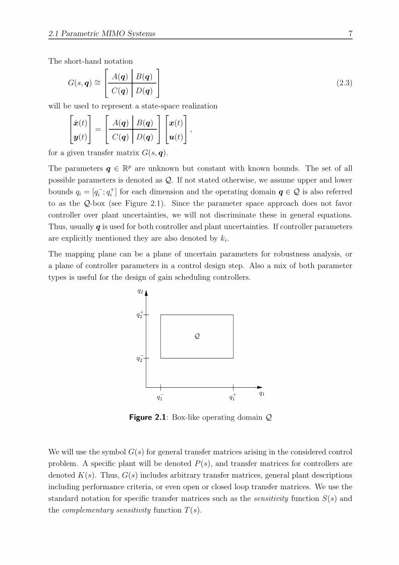
The parameters q ∈ Rp are unknown but constant with known bounds. The set of all
possible parameters is denoted as Q. If not stated otherwise, we assume upper and lower
bounds qi = [q−i ; q+i ] for each dimension and the operating domain q ∈ Q is also referred
to as the Q-box (see Figure 2.1). Since the parameter space approach does not favor
controller over plant uncertainties, we will not discriminate these in general equations.
Thus, usually q is used for both controller and plant uncertainties. If controller parameters
are explicitly mentioned they are also denoted by ki.
The mapping plane can be a plane of uncertain parameters for robustness analysis, or
a plane of controller parameters in a control design step. Also a mix of both parameter
types is useful for the design of gain scheduling controllers.
q1q−
1 q+
1
q2
q−
2
q+
2
Q
Figure 2.1: Box-like operating domain Q
We will use the symbol G(s) for general transfer matrices arising in the considered control
problem. A specific plant will be denoted P (s), and transfer matrices for controllers are
denoted K(s). Thus, G(s) includes arbitrary transfer matrices, general plant descriptions
including performance criteria, or even open or closed loop transfer matrices. We use the
standard notation for specific transfer matrices such as the sensitivity function S(s) and
the complementary sensitivity function T (s).

8 Control Specifications and Uncertainty
2.1.1 MIMO Specifications
The main objective of the parameter space approach is to map specifications relevant
for dynamic systems (2.1) and (2.2) into the parameter space or into a parameter plane.
Apart from stability, the most important objective of a control system is to achieve certain
performance specifications. One way to describe these performance specifications is to use
the size of certain signals of interest. For example, the performance of a regulator could
be measured by the size of the error between the reference and measured signals. The size
of signals can be defined mathematically using norms. Common norms are the Euclidean
vector norms
||x||1 :=n∑
i=1
|xi|, ||x||2 :=
√√√√
n∑
i=1
|xi|2, ||x||∞ := max1≤i≤n
|xi|.
The performance of a control system with input and output signals measured by one
of the above norms, not necessarily the same, can be evaluated by the induced matrix
norms. The most prominent matrix norms used in control theory are the H∞ and H2
norms, which will be considered in Section 2.4.1 and Section 2.4.6, respectively.
2.1.2 MIMO Properties
MIMO systems exhibit some properties not known for single-input single-output (SISO)
systems. These differences make it difficult to apply standard SISO design guidelines to
MIMO systems, e.g., for eigenvalues or loop shapes. At least care has to be taken when
simply using these rules.
While for a SISO system the behavior can be characterized by the gain and phase for
a single channel, these entities depend on the direction of the input for MIMO systems.
The same applies to eigenvalues. While eigenvalues can be used to describe the behav-
ior of a SISO system effectively, for MIMO systems the directionality of the associated
eigenvectors becomes important. This can be also seen from a design point of view. The
eigenvalues of a controllable system with available state information can be moved to
any desired location using Ackermann’s formula [Ackermann 1972]. For multivariable
systems there are additional degrees of freedom that can be used to shape the closed-loop
eigenvectors or other design specifications.
It is a well known fact that right half plane (RHP) zeros impose fundamental limitations
on control of SISO systems. While these zeros can be found by inspection of the numerator
of the transfer function of a SISO system, this does not hold for MIMO systems. Although
all elements of a transfer matrix G(s) are minimum-phase, RHP zeros may exist for the
overall multivariable system.

2.2 Symbolic State-Space Descriptions 9
The role of RHP zeros is further emphasized by some design methods, e.g., successive
loop closure, where zeros can arise during intermediate steps. Nevertheless sometimes we
can take advantage of the additional degree of freedom found in MIMO systems to move
most of the deteriorating effect of an RHP zero to a particular output channel.
2.2 Symbolic State-Space Descriptions
All methods and algorithms presented in this thesis require a symbolic state-space de-
scription. In particular the mapping equations for control system specifications presented
in Chapter 3 are based on a parametric, linear state-space description of the considered
system as in (2.1). The purpose of this section is to present an algorithm that calculates
a symbolic state-space description from a given symbolic transfer function, because this
is essential for the methods developed in this thesis.
Such a system description can be obtained by first-principle modeling such as Lagrange
functions or balance equations, where it might be necessary to symbolically linearize
the equations. Note that this linearization preserves the parametric dependency on the
uncertain parameters q. The references Otter [1999], Tiller [2001] give a good introduction
to object oriented modeling where the used software symbolically transforms and modifies
the system description.
While a parametric transfer matrix is easily obtained from a state-space description by
evaluating the symbolic expression G(s, q) = C(q)(sI−A(q))−1B(q)+D(q), the opposite
is much more involved.
For SISO systems or systems with either a single input or output, a canonical form
provides a minimal realization. Particular variants are the controllable and observable
canonical form [Chen 1984, Kailath 1980]. These canonical forms can be easily obtained
in symbolic form from the coefficients of a transfer function.
Consider a multivariable transfer matrix G(s). One way to obtain a state-space description
is to form canonical forms of all transfer functions gij(s) and combine them to get a model
with input-output relation equivalent to the considered transfer matrix G(s). This model
will be nonminimal, i.e., it contains spurious states, which are non-controllable or non-
observable, or both.
For MIMO systems the dimension of a minimal realization is exactly the McMillan de-
gree [Chen 1984]. There exist standard methods to determine a minimal realization for
a numerical state-space model. Unfortunately these algorithms are not transferable to
symbolic transfer matrix descriptions.

10 Control Specifications and Uncertainty
2.2.1 Transfer Function to State-Space Algorithm
Besides system representations in state-space and transfer function form, a matrix frac-
tion description (MFD) is another useful way of representing a system. Actually these
models are the keystone of all linear fractional representation (LFR) based robust control
methods, where the idea is to isolate the uncertainty from the system inside a single block.
The aim here is to present a symbolic algorithm. It will be formulated using right coprime
factorization. A dual left coprime version is possible, but does not provide any advantages
over the presented one.
Any transfer matrix G(s) can be written as a right or left matrix fraction of two polynomial
matrices,
G(s) = Nr(s)Mr(s)−1, (2.4a)
G(s) = Ml(s)−1Nl(s). (2.4b)
The numerator matrices Nr(s) and Nl(s) have the same dimension as the transfer ma-
trix G(s), whereas the denominator matrices Mr(s) and Ml(s) are square matrices of
matching dimension. Special variants are coprime factorizations, which will be discussed
later in Section 2.2.2.
A right (left) MFD for a given transfer matrix G(s) ∈ Rl,m is easily obtained as follows.
Determine the polynomial denominator matrix M(s) as a diagonal matrix, where the
entries mii are the least common multiple of all denominator polynomials in the i-th
column (row) of G(s), i.e.,
mii = lcm(den g1i, den g2i, . . . , den gli), i = 1, . . . , m, (2.5a)
and for left MFDs we use
mii = lcm(den gi1, den gi2, . . . , den gil), i = 1, . . . , l. (2.5b)
The fraction-free numerator matrices Nr(s) and Nl(s) are then determined by simply
evaluating
Nr(s) = G(s)Mr(s), (2.6a)
Nl(s) = Ml(s)G(s). (2.6b)
Having found a column-reduced MFD a state-space realization can be determined using
the so-called controller-form [Kailath 1980]. The algorithm presented here will work for
proper and strictly proper systems.

2.2 Symbolic State-Space Descriptions 11
Given a right MFD G(s) = Nr(s)Mr(s)−1, the input-output relation y(s) = G(s)u(s) can
be rewritten as
Mr(s)ξ(s) = u(s), (2.7a)
y(s) = Nr(s)ξ(s), (2.7b)
where ξ(s) is the so-called partial state.
The polynomial matrices Nr(s) and Mr(s) are now decomposed as
Mr(s) = MhcS(s) + MlcΨ(s), (2.8a)
Nr(s) = NlcΨ(s) + NftMr(s). (2.8b)
The decomposition matrices are computed as follows. Let the highest degree of all poly-
nomials in the i-th column of Mr(s) be denoted as ki. The matrix S(s) is diagonal
with S(s) = diag[sk1 , . . . , skm]. Then the matrix Mhc is the highest-column-degree coeffi-
cient matrix of Mr(s).
The term MlcΨ(s) contains the lower-column-degree terms of Mr(s), where Mlc is a coef-
ficient matrix and Ψ(s) a block diagonal matrix:
Ψ(s)T =
1 s · · · sk1−1 0 · · · 0
0 1 s · · · sk2−1 · · · 0
0 0 · · · 0
0 0 · · · 1 s · · · skm−1
.
Output equation (2.8b) is obtained by first computing the direct feedthrough matrix as
Nft = lims→∞
G(s) = lims→∞
Nr(s)Mr(s)−1.
The remaining task is to compute the trailing coefficient matrix Nlc by columnwise coef-
ficient evaluation of NlcΨ(s) = Nr(s) − NftMr(s) for orders of s up to degree ki for the
i-th column.
Having found the decomposition (2.8), a state-space description is now easily obtained by
assembling m integrator chains with ki integrators in the i-th chain. The total order nt
of the system will be given by
nt =
m∑
i=1
ki.

12 Control Specifications and Uncertainty
A basic state-space realization of S(s) is given by
A0 = block diag[Ak1 , . . . , Akm], (2.9a)
B0 = block diag[Bk1 , . . . , Bkm], (2.9b)
C0 = Int. (2.9c)
where An is an n × n Jordan block matrix with corresponding input matrix Bn,
An =
0 1
· · ·· · ·0 1
0
, An ∈ Rn,n,
BTn =
[
0 · · · 0 1]
, Bn ∈ Rn, 1.
The correct input-output behavior is then achieved by closing a feedback loop around the
core integrator chains. The final state-space realization is given by
A = A0 − B0M−1hc Mlc, (2.10a)
B = B0M−1hc , (2.10b)
C = Nlc, (2.10c)
D = Nft. (2.10d)
2.2.2 Minimal Realization
A state-space realization is minimal, if it is controllable and observable, and thus contains
no subsystems that are not controllable or observable, or both.
State-space representations are in general not unique. Nevertheless, minimal state-space
realizations are unique up to a change of the state-space basis. More important, the
number of states is constant and minimal. This minimality is especially important for the
symbolic parameter space approach methods presented in Chapter 3, since they minimize
the computational burden in handling and solving the symbolic equations.
Since the 1960s the minimal realization problem has attracted a lot of attention and
a wide variety of algorithms have emerged, e.g., Gilbert’s approach based on partial-
fraction expansions [Gilbert 1963] or Kalman’s method, which is based on controllability
and observability and reduces a nonminimal realization until it is minimal [Kalman 1963].
Note that an input-output description reveals only the controllable and observable part
of a dynamical system.

2.2 Symbolic State-Space Descriptions 13
Rosenbrock [Rosenbrock 1970] developed an algorithm, which uses similarity transforma-
tions (elementary row or column operations), to extract the controllable and observable,
and therefore minimal subpart of a state-space realization. Variants of this algorithm are
now implemented in Matlab and Slicot.
We will use a similar approach based on MFDs, which directly fits into the results pre-
sented in Section 2.2.1. Consider a right MFD,
G(s) = Nr(s)Mr(s)−1,
with polynomial matrices Nr(s) and Mr(s). We now determine the greatest common right
divisor Rgcd(s) of Nr(s) and Mr(s), such that
Nr(s) = Nr(s)Rgcd(s)−1, (2.11)
Mr(s) = Mr(s)Rgcd(s)−1, (2.12)
and we obtain the right coprime factorization
G(s) = Nr(s)Mr(s)−1. (2.13)
The greatest common right divisor of two polynomial matrices can be found by consec-
utive row operations, or left-multiplication with unimodular matrices, until the stacked
matrix [Mr Nr]T is column reduced. Since all steps in finding Rgcd are either multiplica-
tion or addition of polynomials the algorithm is fraction free and can be easily applied
to parametric matrices. Note that we are not interested in special coprime factorization,
e.g., stable factorization over RH∞. So we can symbolically compute Rgcd(s), e.g., using
Maple.
2.2.3 Example
The above algorithm is illustrated by a small MIMO transfer matrix. Consider the follow-
ing plant [Doyle 1986], which is an approximate model of a symmetric spinning body with
constant angular velocity for a principal axis, and two torque inputs for the remaining
two axes,
G(s) =1
s2 + a2
s − a2 a(s + 1)
−a(s + 1) s − a2
. (2.14)
For this example a right MFD is easily obtained by inspection or using (2.5a) and (2.6a),
Mr(s) =
s2 + a2
s2 + a2
, Nr(s) =
s − a2 a(s + 1)
−a(s + 1) s − a2
. (2.15)

14 Control Specifications and Uncertainty
It is obvious that if by simply following the algorithm given in Section 2.2.1, we would
end up with a state-space description of order four. To minimize the order, we use the
minimal realization procedure of Section 2.2.2.
It turns out that Nr(s) is actually a greatest common right divisor of Mr(s) and Nr(s),
such that Rgcd(s) = Nr(s), and using (2.11), we immediately determine a right coprime
factorization with
Mr(s) =−1
1 + a2Nr(s), Nr(s) = I. (2.16)
We can then proceed with the decomposition (2.8) and using (2.9) and (2.10) we finally
obtain a minimal state-space realization of order two,
G(s) ∼=
0 a
−a 0
1 a
−a 1
1 0
0 1
0 0
0 0
.
2.3 Uncertainty Structures
The main aim of control is to cope with uncertainty.
System models should express this uncertainty,
but a very precise model of uncertainty is an oxymoron.
George Zames
This section contains material on the description of uncertainty for models used in control
system design. While in general the material can be applied to models from different
application areas, e.g., chemical reactors or power plants, the exposition is especially
suited for models of mechanical systems arising in vehicle dynamics.
Control engineers, unless only experiments are used, are working with mathematical mod-
els of the system to be controlled. These models should describe all system responses vital
for the considered system performance. That is, other system properties are neglectable.
Apart from matching the responses of the true plant as close as possible, models should
be simple enough to facilitate design.
By the term uncertainty we will summarize
1. all known variations of the model,
2. differences or errors between models and reality.

2.3 Uncertainty Structures 15
The first type of uncertainty refers to variations of the model due to parameter changes.
For parametric LTI systems a mathematical description is given in (2.1) and (2.2). As
mentioned earlier these system descriptions are easily obtained from first principle model-
ing.
The parameters q are unknown but constant. That is, we assume that the parameters
do not change during a regular operation of the system; or the change is so slow that
they can be treated as quasi-stationary. For parameters which change rapidly or whose
rate of change lies well within the system dynamics special care has to be taken. In this
case the results obtained by treating the parameters as constant or quasi-constant might
be false or misleading. Representing the changing parameters through an unstructured
uncertainty description might be a remedy. Another approach is to utilize the mapping
equations derived in Section 3.4. The stability of a system with an arbitrary fast varying
parameter is analyzed in Example 3.1.
The uncertain parameters might be states of a full-scale model describing the plant be-
havior with respect to input and output variables. For example, the mass of an airplane
can be considered as a fixed parameter for directional control while it is actually a state
of a model and decreasing with fuel consumption used for full flight evaluation.
From a frequency point of view the system knowledge generically decreases with frequency.
While there are system models which are accurate in a specific frequency range, e.g., for
flexible mechanical systems, at sufficiently high frequencies precise modeling is impossible.
This is a consequence of dynamic properties which occur in physical systems.
We propose the following modeling philosophy:
Use the physical knowledge about the plant to include parametric uncer-
tainties as real perturbations with known bounds. Additional uncertainties are
modeled by (unstructured) dynamic uncertainties. Any information, e.g., di-
rectionality, although not expressible as parametric uncertainties about these
uncertainties should be incorporated in analysis and design.
Thus the overall model which includes an uncertainty description is denoted as
G = G(q, ∆), (2.17)
where ∆ represents unstructured uncertainty considered in detail in Section 2.3.3. The
term unstructured is not to be interpreted literally. The uncertainty description might
actually contain some degree of structure. But here it is used as uncertainty which
cannot be described as real parameter variation. The uncertainty description used here
is an extension of pure parametric models used in the classical parameter space approach
to include unstructured uncertainty.

16 Control Specifications and Uncertainty
The frequency domain approaches to robust control, i.e., the popular H∞ and µ control
paradigms, use a different representation of uncertainty. For H∞ robust controllers all
uncertainties have to be captured by a norm-bounded uncertainty description. The model
is described by a nominal plant and H∞ norm-bounded stable perturbations. Thus even
parametric uncertainty, i.e., a detailed parametric model, has to be approximated by a
norm-bounded uncertainty description. Furthermore all uncertainty has to be lumped in
a single uncertainty transfer function or uncertainty block, see Figure 2.2.
∆
G z
u v
w
Figure 2.2: General lumped uncertainty description
While the structured singular value or µ approach tries to alleviate problems associ-
ated with the unstructured uncertainty description by using structured and unstructured
uncertainties, the single uncertainty block ∆ remains. Parametric uncertainties can be
rendered in this single block uncertainty, although some conservativeness is associated
with this approach. See Section 2.3.1 for some comments regarding the transformation of
parametric models into the single block form of Figure 2.2.
Robustness of a control system is not only affected by the plant uncertainty. There are
many other aspects which have to be taken care of, when it comes to successful and robust
operation of a control system. This includes failure of sensor and actuators, fragility of
the implemented controller, physical constraints. Furthermore the opening and closing
of individual loops for a multivariable system can be crucial, especially during manual
start-up or tuning. Nevertheless, robustness refers to robustness with respect to model
uncertainty in this thesis. We will usually try to find a fixed linear controller that robustly
satisfies all design specifications. Apart from robust stability, for real control systems some
performance specification has to be achieved robustly.
2.3.1 Real Parametric Uncertainties
Real parametric uncertainties are lumped into a single vector q ∈ Rp. The general
models for parametric LTI systems were given in (2.1) and (2.2). Since the concept
of real parametric uncertainties is pretty straightforward we will consider some special

2.3 Uncertainty Structures 17
variants and the transformation of a parametric model into a model where all parametric
uncertainty is lumped into a single block.
State perturbations
State perturbations are important in the analysis of robust stability. The most general
state perturbation model is given by the following state-space description
x(t) = (A + Aq(q)) x(t), (2.18)
where Aq(q) is a matrix whose entries are polynomial fractions and Aq(0) = 0 , i.e., A is
the nominal state matrix for q = 0 . Usually only pure polynomial matrices are considered,
since a fractional matrix can be transformed into a polynomial matrix by multiplication
with the least common multiple of all denominators.
Of special interest are representations where all perturbations are combined in a single
block, such as in the general lumped uncertainty description of Figure 2.2. Actually, for
polynomial state perturbations we can find a representation of the form
x(t) =(A + U∆(I − W∆)−1V
)x(t), (2.19)
where ∆ is a diagonal matrix of the form ∆ = diag[q1Im1 , q2Im2 , . . . , qpImp]. The inte-
gers mi are the multiplicities with which the i-th parameter appears in ∆. Figure 2.3
shows a block diagram for state perturbation (2.19).
∆v
Vu
U
W
∫
A
x
Figure 2.3: State perturbation block diagram
If no product terms of parameters are present in (2.18) we can write the system as
x(t) =
(
A +
p∑
i=1
Ai(qi)
)
x(t), (2.20)
where Ai(qi) is the perturbation matrix depending on the parameter qi.

18 Control Specifications and Uncertainty
Affine state perturbations
A further specialization is obtained, if the perturbations are affine in the unknown pa-
rameters, i.e.,
Ai(qi) = Aiqi, i = 1, . . . , p.
Real structured perturbations
An even more special variant of affine state perturbations are the so-called real structured
perturbations.
Thus (2.20) can be written as
x(t) = (A + U∆V ) x(t), (2.21)
where ∆ is a diagonal matrix with real uncertain parameters, ∆ = diag[q1, . . . , qp] ∈ Rp, p.
Lumped real parametric uncertainty
In this section we revisit the general state perturbation representation (2.18)
x(t) = (A + Aq(q)) x(t),
and we investigate how to obtain a lumped real parametric uncertainty description (2.19),
x(t) = (A + U∆(I − W∆)−1V ) x(t),
where all perturbations are inside a single block ∆.
For fractional, polynomial parameter dependency such a representation can be found by
extracting all non-reducible factors and representing them using a diagonal uncertainty
matrix with the individual factors as elements, e.g., using a tree decomposition [Barmish
et al. 1990a]. Another technique uses Horner factorization [Varga and Looye 1999]. See
[Magni 2001] for an overview of realization and order reduction algorithms.
Representation (2.19) is shown as a block diagram in Figure 2.3. From this block diagram
it becomes obvious that the uncertainty block ∆ can be pulled out and the system can
be put into the lumped uncertainty form of Figure 2.2. This is shown in Figure 2.4. The
transfer function for the uncertainty block from output u(s) to input v(s) is
Guv(s) = (I − W∆)−1V (sI − A)−1U. (2.22)

2.3 Uncertainty Structures 19
∆
W
∫
A
Ux
V
vu
Figure 2.4: Lumped state perturbation
Example 2.1 Consider the following system with state perturbation:
x(t) =
0 1
−1 −2
+
−q1 + q1q2 q1q2
q2 q1 − q2
x(t) (2.23)
This representation can be reduced to the following minimal form:
∆ =
q1
q1
q2
q2
, W =
0
0
−1 1 0
0
,
U =
1 0 1 0
0 1 0 1
, V T =
−1 0 0 1
0 1 0 −1
�
2.3.2 Multi-Model Descriptions
A multi-model description consists of a finite number of fixed model descriptions of the
form
x(t) = Aix(t) + Biu(t), y(t) = Cix(t) + Diu(t), i ∈ 1, . . . , p, (2.24)

20 Control Specifications and Uncertainty
where p is the number of individual models. Thus a multi-model description usually does
not contain any parameters. Multi-model descriptions are easily treated in the parameter
space approach by consecutively mapping a specification for each model.
2.3.3 Dynamic Uncertainty
The term dynamic uncertainty might be a bit misleading in the sense that all other
uncertainty structures presented in Section 2.3 are describing uncertainties of dynamic
systems. By dynamic uncertainty we refer to uncertainties whose underlying dynamics
are not precisely known and are possibly varying within known bounds.
Dynamic uncertainty operators are often associated with modeling errors that are not
efficiently described by parametric uncertainty. Unmodeled dynamics and inaccurate
mode shapes of aero-elastic models [Lind and Brenner 1998] are examples of modeling
errors that can be described with less conservatism by dynamic uncertainties than with
parametric uncertainties. These dynamic uncertainties are typically complex in order to
represent errors in both magnitude and phase of signals.
The set of unstructured uncertainties ∆ is given as all stable transfer functions (rational
or irrational) of appropriate dimension that are norm bounded:
∆ := {∆ ∈ RH∞, ||∆|| < l(ω)}. (2.25)
We will use the H∞ norm throughout the thesis (see Section 2.4.1 for a review of the H∞
norm) and usually the following normalization condition holds: ||∆||∞ ≤ 1. This normal-
ization can always be enforced by using suitable weighting functions.
There are several possibilities how to describe plant perturbations using unstructured
uncertainties ∆. The most prominent and most intuitive are the (output) multiplicative
and additive perturbations:
Gp(s) = G(s) + Wa(s)∆(s), (2.26)
Gp(s) = (I + ∆(s)Wo(s)) G(s), (2.27)
where Wa(s) and Wo(s) are weights such that ||∆(s)||∞ ≤ 1. See Figure 2.5.
Similar plant perturbations are inverse additive uncertainty, inverse multiplicative output
and (inverse) multiplicative input uncertainty. Another common form is coprime factor
uncertainty:
Gp(s) = (Ml + ∆M)−1(Nl + ∆N), (2.28)
where Ml, Nl is a left coprime factorization of the nominal plant model. This uncertainty
description, suggested by McFarlane and Glover [1990], is mainly used in an H∞ norm

2.3 Uncertainty Structures 21
Wa ∆
G G
Wo ∆
Figure 2.5: Additive and multiplicative output uncertainty
loop-shaping procedure, where the open-loop shapes are shaped by weights and the ro-
bustness of the resulting plant to this type of uncertainty is maximized. Usually, no
problem-dependent uncertainty modeling is used in this approach, see [Skogestad and
Postlethwaite 1996] for a thorough treatment.
For plants with different physically motivated perturbations, e.g., input and output mul-
tiplicative uncertainty, it is possible to lump all uncertainties into a single perturbation,
see Figure 2.2. Unfortunately even for unstructured perturbations the resulting overall
uncertainty ∆ is block-diagonal and therefore structured. A straightforward application
of the small-gain theorem (see Theorem 2.2 in Section 2.4.1) will be obviously conserva-
tive, because the system is checked for a much larger set of uncertainties which actually
cannot appear in the real system.
Back in 1982, Doyle and Safonov introduced simultaneously equivalent entities to measure
the robustness margin of a system with respect to structured uncertainties. For a general
system as in Figure 2.2 the so-called structured singular value µ is defined as
µ∆(G(s)) :=1
min{σ(∆) | det[I − G(s)∆] = 0} ,
where σ is the maximal singular value (see Section 2.4.1). The value µ∆(G(s)) is a simple
scalar measure of the smallest structured uncertainty which destabilizes the feedback
system.
The µ approach has been extended to the synthesis of robust controllers and there are
several related toolboxes. Yet, the exact computation of µ is not possible except for
special cases. Thus all available software tries to compute meaningful bounds for µ. This
emphasizes the goal of this thesis to treat real parameter variations directly and only
represent them into a lumped uncertainty ∆, if the parameters are changing fast or their
number is large and we want to refrain from gridding.
Another rational of this approach comes from the fact that µ with respect to pure real
uncertain parameters is discontinuous in the problem data [Barmish et al. 1990b]. That
is, for small changes of the nominal system, maybe due to a neglected parameter, the
stability margin might be subject to large, discontinuous changes. Put in other words,

22 Control Specifications and Uncertainty
for a specific model the real µ is not a good indicator of robustness because it might
deteriorate for an infinitesimal perturbation of the considered plant.
2.4 MIMO Specifications in Control Theory
This section reviews the various specifications and objectives relevant for design and ana-
lysis of multivariable control systems. All specifications will be formulated using algebraic
Riccati equations (AREs) or Lyapunov equations. See Section 3.2 for an introduction to
AREs. While there will be no special notation for parametric dependencies, the considered
systems might depend on several real parameters q ∈ Rp.
The specifications are briefly motivated from a general control theoretic point of view.
Special attention is given to reasons why it might be advantageous to include these specifi-
cations into the parameter space approach. For motivation of the specifications presented
in this section see for example [Boyd et al. 1994] or [Scherer et al. 1997].
Apart from the introduction of the specifications, the main aim of this section is to
present them in a mathematical formulation, that is tractable for the mapping equations
developed in Chapter 3.
2.4.1 H∞ Norm
Probably the most prominent norm used in control theory to date is the H∞ norm.
The H∞ norm of a transfer function G(s) is defined as the peak of the maximum singular
value of the frequency response
||G(s)||∞ := supω
σ(G(jω)), (2.29)
where σ is the largest singular value or maximal principal gain of an asymptotically stable
transfer matrix G(s). Note that (2.29) defines the L∞ norm, if the stability requirement
is dropped.
There are several interpretations of the H∞ norm. A signal related interpretation is given
by
||G||∞ = supw 6=0
||Gw||2||w||2
.
Consider a scalar transfer function G(s), then the infinity norm can be interpreted as
the maximal distance of the Nyquist plot of G(s) from the origin or as the peak value
of the Bode magnitude plot of |G(jω)|. In that sense, frequency response magnitude
specifications [Odenthal and Blue 2000] can be recast as scalar H∞ norm problems.

2.4 MIMO Specifications in Control Theory 23
For SISO systems the H∞ norm is simply the maximum gain of the transfer function,
whereas for MIMO systems it is the maximum gain over all directions. Thus the H∞
norm takes the directionality of MIMO systems into account.
For MIMO systems, the H∞ norm describes the maximum amplitude of the steady state
response for all possible unit amplitude sinusoidal input signals. In the context of stochas-
tic input signals, the H∞ norm can be interpreted as the square root of the maximal energy
amplification for all input signals with finite energy.
Note that unlike the induced matrix norms ||A||p, which are related to vector norms ||x||p,the norms used for matrix functions are not directly related to the namesake signal norms.
For example, the L1 norm is another norm, frequently used for LTI systems,
||G||1 := supw 6=0
||Gw||∞||w||∞
.
The H∞ norm can be used to evaluate nominal stability of a system without uncertainty.
By evaluating the H∞ norm of special transfer functions, e.g., a weighted sensitivity
function, performance and robustness of a control system can be assessed. We will show
how to incorporate the latter feature into the PSA in the next chapter.
Based on the control theoretic useful mathematical properties the so-called H∞ prob-
lem was defined by Zames [1981]. Using the general control configuration of Figure 2.6,
the standard H∞ optimal control problem is to find all stabilizing controllers1 K which
minimize
||Fl(P, K)||∞, (2.30)
where Fl(P, K) := P11 +P12K(I −P22K)−1P21 is a lower linear fractional transformation.
Often one is content with a suboptimal controller which is close to the optimal. Then
the H∞ control problem becomes: given a γ > γmin, where γmin is the minimal, achievable
value, find all stabilizing controllers K such that
||Fl(P, K)||∞ < γ. (2.31)
Following [Zames 1981] a number of different formulations and solutions were developed.
One successful approach to solve H∞ control problems involves AREs, see [Doyle et al.
1989, Petersen 1987]. The ARE based algorithm of Doyle et al. [1989] is summarized in
[Skogestad and Postlethwaite 1996, p. 367]. The formulation based on AREs will become
important in Chapter 3 when we derive mapping equations for H∞ norm specifications.
1We use K for controllers to avoid ambiguity with the output-state matrix C

24 Control Specifications and Uncertainty
P
K
z
u v
w
Figure 2.6: General control configuration
Hence we do not pursue the automatic solution of (2.31), since we are trying to incor-
porate H∞ criteria into the PSA. Nevertheless the achievable level γ is of interest when
mapping an H∞ specification.
The following theorem, which is known as the bounded real lemma [Boyd et al. 1994],
provides an important link between H∞ control problems and AREs and will therefore
become important in Chapter 3. This theorem, besides its theoretical significance, is often
used as a preparation for the solution of the H∞ problem.
Theorem 2.1 Bounded real lemma
Consider a linear system with transfer function G(s) and corresponding minimal
state-space realization G(s) = C(sI − A)−1B + D. Then the following statements
are equivalent:
(i) G(s) is bounded-real, i.e., G(s)∗G(s) ≤ I, ∀ Re s > 0;
(ii) G(s) is non-expansive, i.e.,∫ τ
0
y(t)T y(t)dt ≤∫ τ
0
u(t)T u(t)dt, τ ≥ 0;
(iii) the H∞ norm of G(s) with A being stable, σ(D) < γ, and γ = 1 satisfies
||G(s)||∞ ≤ γ;
(iv) the algebraic Riccati equation
γXBS1
r B∗X +γC∗S1
l C−X(A−BS1
r D∗C)− (A−BS1
r D∗C)∗X = 0 , (2.32)
with γ = 1 has a Hermitian solution X0 such that all eigenvalues of the ma-
trix A − BB∗X0 lie in the open left half-plane, where Sr = (D∗D − γ2I)
and Sl = (DD∗ − γ2I).
�
2.4 MIMO Specifications in Control Theory 25
Note: The equivalence of (iii) and (iv) in Theorem 2.1 was stated using the parameter γ
such that we can map different performance levels γ for an H∞ norm specification into
parameter space in Chapter 3.
All robust stability conditions for uncertain systems using the H∞ norm can be based on
the following rather general result [Zhou et al. 1996].
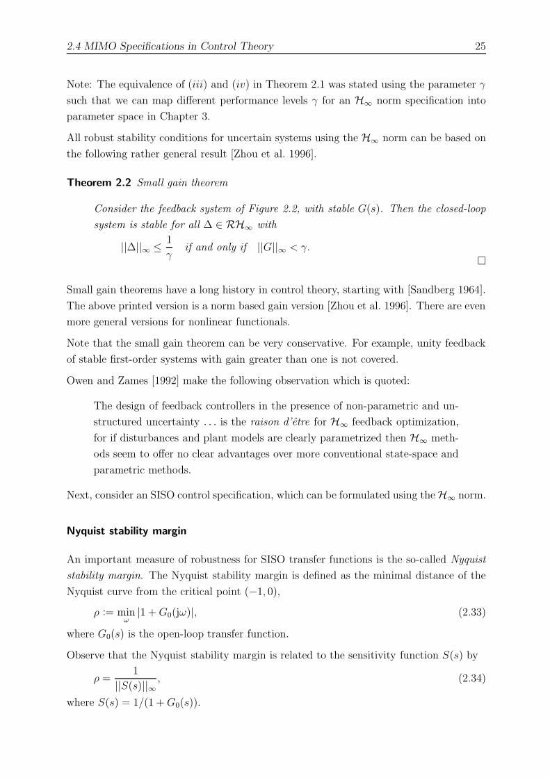
Theorem 2.2 Small gain theorem
Consider the feedback system of Figure 2.2, with stable G(s). Then the closed-loop
system is stable for all ∆ ∈ RH∞ with
||∆||∞ ≤ 1
γif and only if ||G||∞ < γ.
�
Small gain theorems have a long history in control theory, starting with [Sandberg 1964].
The above printed version is a norm based gain version [Zhou et al. 1996]. There are even
more general versions for nonlinear functionals.
Note that the small gain theorem can be very conservative. For example, unity feedback
of stable first-order systems with gain greater than one is not covered.
Owen and Zames [1992] make the following observation which is quoted:
The design of feedback controllers in the presence of non-parametric and un-
structured uncertainty . . . is the raison d’etre for H∞ feedback optimization,
for if disturbances and plant models are clearly parametrized then H∞ meth-
ods seem to offer no clear advantages over more conventional state-space and
parametric methods.
Next, consider an SISO control specification, which can be formulated using the H∞ norm.
Nyquist stability margin
An important measure of robustness for SISO transfer functions is the so-called Nyquist
stability margin. The Nyquist stability margin is defined as the minimal distance of the
Nyquist curve from the critical point (−1, 0),
ρ := minω
|1 + G0(jω)|, (2.33)
where G0(s) is the open-loop transfer function.
Observe that the Nyquist stability margin is related to the sensitivity function S(s) by
ρ =1
||S(s)||∞, (2.34)
where S(s) = 1/(1 + G0(s)).

26 Control Specifications and Uncertainty
2.4.2 Passivity and Dissipativity
The roots of passivity as a control concept can be traced back to the 1940’s, when re-
searchers in the Soviet Union applied Lyapunov’s methods to stability of control systems
with a nonlinearity. But it took up to 1971, when Willems [1971] formulated the notion
of passivity in a system theoretic framework.
The most striking feature of passivity is that any interconnection of passive systems is
passive. Figure 2.7 illustrates some connections of passive subsystems which comprise a
passive system.
Passive
System 1
Passive
System 2 y2
y
y1
u
w1
u1 Passive
System 1
Passive
System 2 u2
w2
y1
y2
Figure 2.7: Interconnection of passive systems
This fact can be used to design robust controllers by subdividing the complete control
system into passive subsystems and designing a passive controller. If the plant is not
passive, a suitable approach is to fix a controller which leads to a passive controlled sub-
system. On top of this, additional performance enhancing controllers can be determined
which preserve passivity. This approach is similar to the classical feedback - feedforward
filter design steps of many control design approaches.
Since passivity is also defined for nonlinear systems this concept can be applied to control
systems with either nonlinear plant or controller. This approach is easily extended to
parametric robustness by checking or guaranteeing that a system is passive under all
parameter variations.
We will consider quadratic MIMO systems, i.e., the dimension of the input equals the
output dimension. This is a mandatory assumption for passivity. For dissipativity, which
can be seen as the generalization of passivity, this is not necessary, see Definition 2.1 on
page 28. Nevertheless, commonly used dissipativity definitions, e.g., (2.40), assume that
the system is quadratic.
For a linear system passivity is equivalent to the transfer matrix G(s) being positive-real,
which means that
G(s) + G(s)∗ ≥ 0 ∀ Re s > 0. (2.35)

2.4 MIMO Specifications in Control Theory 27
In the time-domain a system is said to be passive if∫ τ
0
u(t)T y(t) dt ≥ 0, ∀ τ ≥ 0, x(0) = 0 . (2.36)
Passivity can be interpreted for physical systems, if the term u(t)T y(t) is a power, e.g.,
current and voltage for electrical and co-located force and velocity for mechanical systems.
Equation (2.36) then says that the difference between supplied and withdrawn energy is
positive.
For SISO transfer functions passivity can be checked graphically by plotting the Nyquist
diagram. If the resulting curve lies in the right half plane then the system is passive.
The following lemma [Anderson 1967] translates the frequency-domain condition (2.35)
into a matrix condition which will lead to mapping equations.
Lemma 2.3 Positive Real Lemma
Consider a linear, time-invariant system G(s) = C(sI − A)−1B + D, with (A, B)
stabilizable, (A, C) observable and D + D∗ nonsingular. Then G(s) is positive real
or passive, if there are matrices L, W , and X = X∗ > 0, such that
A∗X + XA = −L∗L, (2.37a)
XB − C∗ = −L∗W, (2.37b)
D + D∗ = W ∗W. (2.37c)
�
Using elementary matrix operations the unknown matrices L and W can be eliminated
to give the ARE
A∗X + XA + (XB − C∗)(D + D∗)−1(XB − C∗)∗ = 0 . (2.38)
Condition (2.35) is equivalent to the following statement: There exists X = X ∗ satisfying
the ARE (2.38). This equivalence can be found in [Willems 1971]. Using Theorem 3.1
the equivalence between (2.35) and the non-existence of pure imaginary eigenvalues of a
Hermitian matrix can be established. This was first done in [Lancaster and Rodman 1980].
Equation (2.38) will be used to obtain mapping equations for passivity in Chapter 3.
In the preceding formulations a non-zero feedthrough D with D + D∗ nonsingular was
assumed. It turns out that for strictly-proper systems with D + D∗ singular matters
become more difficult. Equation (2.38) disintegrates into:
A∗X + XA < 0, (2.39a)
XB − C∗ = 0 . (2.39b)

28 Control Specifications and Uncertainty
The linear matrix inequality (LMI) (2.39a) has to hold, while the constraint (2.39b) is
satisfied. Because this system of equations and inequalities does not fit into the ARE
framework we will use the more general dissipativity in Chapter 3 in order to develop
mapping equations for passivity.
A system is said to have dissipation η if∫ τ
0
(u(t)T y(t) − ηu(t)T u(t)) dt ≥ 0, ∀ τ ≥ 0, x(0) = 0 . (2.40)
Thus passivity corresponds to non-negative dissipation. A system has dissipativity η, if
the following ARE has a Hermitian solution
A∗X + XA + (XB − C∗)(D + D∗ − 2ηI)−1(XB − C∗)∗ = 0 . (2.41)
The AREs (2.38) and (2.41) will be used later to derive algebraic mapping equations
for LTI systems. Thus these AREs allow to incorporate passivity and dissipativity for LTI
systems into the parameter space approach.
As mentioned earlier, the concept of dissipativity carries over to nonlinear systems. In
order to do this we need a more general definition of dissipativity [Willems 1971].
Definition 2.1 Let x(t) = f(x(t), u(t)), y(t) = h(x(t), u(t)) be a system, with state x(t),
input u(t) and output y(t). This system is dissipative with respect to a supply rate S, if
there is a (storing) function V (x), such that
V (x(τ)) − V (x(0)) ≤∫ τ
0
S(u(t), y(t)) dt, (2.42)
is satisfied. �
Note that the latter definition is formulated in terms of the internal state x(t), while the
formulation in (2.40) is related to the input-output behavior of a system. For quadratic
systems, where the input and output dimensions are equal, this definition can now be
specialized using particular supply rates [Sepulchre et al. 1997].
Definition 2.2 Let x(t) = f(x(t), u(t)), y(t) = h(x(t), u(t)) be a system, with state x(t),
input u(t) and output y(t). This system is α−input dissipative, β−output dissipative,
if (2.42) is satisfied with S(u, y) = uT y − α||u||2, S(u, y) = uT y − β||y||2, respectively.
�
Definition 2.2 defines the general α-input and β-output dissipativity. There is no as-
sumption on the values of these parameters. In comparing Definition 2.2 with (2.40)
we conclude that (2.40) corresponds to η-input passivity. After (2.40) we noted that
passivity corresponds to non-negative dissipation η. While the interconnection properties
of passive systems are well-known, we are now interested in feedback interconnections of
dissipative systems used in Definition 2.2.

2.4 MIMO Specifications in Control Theory 29
Theorem 2.4 [Sepulchre et al. 1997]
Let two systems be feedback interconnected as in the right part of Figure 2.7. The
closed loop system is asymptotically stable, if System 1 is α-input dissipative, Sys-
tem 2 is β-output dissipative, and α + β > 0 holds.
�
This theorem assures that the feedback interconnection of two purely passive systems,
i.e., α = β = 0, is stable. We will use Theorem 2.4 and Definition 2.2 to apply the
passivity results to famous results for nonlinear control systems in Section 2.4.4.
Remark 2.1 Quadratic Constraints
Both H∞ norm and dissipativity specifications fit into the more general framework
of quadratic constraints of the form
∫ τ
0
y(t)
u(t)
T
Q S
ST R
y(t)
u(t)
dt ≤ 0, ∀ τ ≥ 0, x(0) = 0 . (2.43)
�
We will consider an even more general set of specifications, which includes (2.43) in
Section 2.5.
2.4.3 Connections between H∞ Norm and Passivity
For SISO systems both the H∞ norm and the passivity condition resemble classical gain
and phase conditions. They are even more related and can be even translated into each
other.
Using the bilinear Cayley transformation
G(s) = (I − G(s))(I + G(s))−1, with det [I + G(s)] 6= 0, (2.44)
the following equivalence holds [Anderson and Vongpanitlerd 1973, Haddad and Bernstein
1991].
Theorem 2.5
(i) G(s) is positive-real, i.e., G(s) + G(s)∗ ≥ 0 ∀ Re s > 0;
(ii) ||G(s)||∞ < 1.
�

30 Control Specifications and Uncertainty
By Theorem 2.5 a positive realness condition can be recast as an H∞ norm condition
and vice versa. The application of this theorem in the time-domain is facilitated by the
following conversion.
Let G(s) have the state-space realization
G(s) ∼=
A B
C D
,
then a realization for G(s) is given by
G(s) ∼=
A − B(I + D)−1C B(I + D)−1
−2(I + D)−1C (I − D)(I + D)−1
. (2.45)
If we want to apply the results in the opposite direction, we can exchange the sym-
bols G and G, since the Cayley transformation is bilinear, i.e., the converse of transfor-
mation (2.44) is simply G(s) = (I − G(s))(I + G(s))−1 with det[I + G(s)] 6= 0.
For systems with a static feedthrough matrix D which satisfies det[I + D] = 0 the con-
version based on (2.45) fails. In this case, the transformation from a positive-real to
an H∞ norm condition can be done by using a positive realness preserving congruence
transformation G(s) → G(s) = V ∗G(s)V :
G(s) ∼=
A BV
V ∗C V ∗DV
,
where V is a nonsingular matrix such that det[I +V ∗DV ] 6= 0. For the converse transfor-
mation from an H∞ norm to a positive-real condition we can use a sign matrix transfor-
mation G(s) → G(s) = G(s)S, where S is a sign matrix such that det[I + DS] 6= 0 [Boyd
and Yang 1989].
2.4.4 Popov and Circle Criterion
Although this thesis is mainly concerned with specifications for LTI systems, the presented
theory can be applied to criteria for nonlinear systems. Absolute stability theory allows
to analyze the stability of an LTI system in the feedforward path interconnected with
a static nonlinearity in the feedback path. There are two well-known variants, namely
the Popov and Circle criterion, which can be formulated as the feedback of two passive
systems [Khalil 1992, Kugi and Schlacher 2002].
Both criteria assume a sector nonlinearity. Figure 2.8 shows the general feedback structure
for absolute stability, where Ψ(y) represents the nonlinearity.

2.4 MIMO Specifications in Control Theory 31
Circle criterion
Consider the feedback structure given in Figure 2.8 where the multivariable static non-
linearity Ψ(y) satisfies the sector condition
(Ψ(y) − K1y)T (Ψ(y) − K2y) ≤ 0, (2.46)
with K1, K2 matrices which satisfy K2 − K1 > 0. Thus the nonlinearity is contained in
the sector K1, K2. Note that apart from the positive definiteness of K2 −K1 there are no
further assumptions such as SISO.
[
A B
C 0
]
Ψ(y)
u y
Figure 2.8: Feedback structure for absolute stability
Using an equivalence transformation the feedback loop in Figure 2.8 can be put in the
form Figure 2.9. It can be shown that the nonlinear System 2 in Figure 2.9 is β-output
dissipative, with β = 1. From Theorem 2.4 then follows the Circle criterion, see [Khalil
1992, Vidyasagar 1978]:
Theorem 2.6 Circle Criterion
Consider the feedback structure in Figure 2.8 with a sector nonlinearity Ψ(y) which
satisfies (2.46). The closed loop is absolutely stable, if the LTI system
x(t) = (A − BK1C)x(t) + Bu(t)
y(t) = (K2 − K1)Cx(t)(2.47)
is α-input dissipative with α > −1.
�

32 Control Specifications and Uncertainty
[
A B
C 0
]
K
K−1Ψ(y)
K1
K1
System 2
System 1
Figure 2.9: Equivalent feedback loop for circle criterion
Theorem 2.6 can now be formulated as an ARE using the µ-input dissipativity ARE (2.41)
with µ = −1,
XBB∗X + X(2A − BKsC) + (2A − BKsC)∗X + C∗K∗dKdC = 0 , (2.48)
where Ks = K1 + K2, and Kd = K2 − K1.
The condition for absolute stability given in Theorem 2.6 is sufficient. Because this does
not imply necessity there might be considerable conservativeness. If we sacrifice the
generality of the multivariable sector condition (2.46), we can derive sufficient conditions
which can be much tighter. This leads to the Popov criterion considered next.
Popov criterion
For the Popov criterion the considered nonlinearity Ψ(y) is a simple decentralized func-
tion Ψj = Ψj(yj) with
0 ≤ kj ≤ Ψj(yj), j = 1, . . . , m, (2.49)
i.e., K = diag(ki) ∈ Rm, m.

2.4 MIMO Specifications in Control Theory 33
Using an equivalence transformation similar to the one considered for the circle criterion
the nonlinearity Ψ(y) can be embedded into a dissipative subsystem. The decentralized
constraint on the nonlinearity offers some freedom, which can be used to include the
factor (µs + 1)−1 in the nonlinear subsystem while still maintaining dissipativity. This
additional degree of freedom µ can be chosen arbitrarily.
Theorem 2.7 Popov criterion
Consider the feedback structure in Figure 2.8 with a stationary, sector nonlinear-
ity Ψ(y) which satisfies (2.49). The closed loop is absolutely stable, if there is a µ ∈ R
such that the LTI system
x(t) = Ax(t) + Bu(t),
y(t) = KC((I + µA)x(t) + µBu(t)),(2.50)
is α-input dissipative with α > −1.
�
Let C = KC(I + µA), then the ARE related to Theorem 2.7 is given by
A∗X + XA + (XB − C∗)(2I + µKCB + µB∗C∗K∗)−1(XB − C∗)∗ = 0 . (2.51)
2.4.5 Complex Structured Stability Radius
The complex structured stability radius of the system
x(t) = (A + U∆V )x(t) (2.52)
is defined by
rC = inf{
||∆|| : Λ(A + U∆V ) ∩ C+ 6= ∅
}
, (2.53)
where ∆ is a complex matrix of appropriate dimension, C+ denotes the closed right half
plane, and ||∆|| is the spectral norm of ∆.
Lemma 2.8
Let G(s) = V (sI − A)−1U . Then
rC(A, U, V ) = ||G||−1∞ . (2.54)
�

34 Control Specifications and Uncertainty
A proof can be found in [Hinrichsen and Pritchard 1986]. Thus the determination of the
complex structured stability radius is equivalent to the computation of the H∞ norm of
a related transfer function.
Note that not all possible perturbations are expressible with a single block perturba-
tion (2.52), e.g.,
x(t) =
−1 0
2 −2
+
0 δ1
δ2 δ3
x(t).
2.4.6 H2 Norm Performance
The H2 norm is a widely used performance measure that allows to incorporate time-
domain specifications into control design. The H2 norm of a stable transfer matrix G(s)
is defined as
||G(s)||2 :=
(
trace1
2π
∫ ∞
−∞
G(jω)∗G(jω)dω
)1/2
.
The above norm definition can be used for generic square integrable functions on the
imaginary axis and is then called L2 norm. Thus, strictly speaking without the stability
condition, we are mapping the L2 norm instead of the H2 norm.
The H2 norm arises, for example, in the following physically meaningful situation. Let
the system input be zero-mean stationary white noise of unit covariance. Then, at steady
state, the variance of the output is given by the square of the H2 norm. This can be seen
from the general definition of the root mean square response norm for systems driven by
a particular noise input with power spectral density matrix Sw:
||G||rms,s :=
(
trace1
2π
∫ ∞
−∞
G(jω)∗Sw(jω)G(jω)dω
)1/2
.
The H2 norm is only finite, if the transfer matrix G(s) is strictly proper, i.e., the direct
feedthrough matrix D = 0 (or D(q) = 0 ). Hence we assume D = 0 in this subsection,
which is a valid assumption for almost any real physical system.
By Parseval’s theorem, the H2 norm can be expressed as
||G||2 =
(
trace
∫ ∞
0
H(t)T H(t)dt
)1/2
, (2.55)
with H(t) = CeAtB being the impulse matrix of G(s) = C(sI − A)−1B.

2.4 MIMO Specifications in Control Theory 35
From this follows
||G||22 = trace [BT
∫ ∞
0
eAT tCT CeAtdt B]
= trace [BT WobsB], (2.56)
where
Wobs :=
∫ ∞
0
eAT tCT CeAtdt
is the observability Gramian of the realization, which can be computed by solving the
Lyapunov equation
AT Wobs + WobsA + CT C = 0 . (2.57)
Alternatively a dual output-controllable formulation exits for ||G||22, which involves the
controllability Gramian Wcon,
||G||22 = trace [CWconCT ], (2.58)
where Wcon can be determined from
AWcon + WconAT + BBT = 0 . (2.59)
The H2 norm is different from the specifications presented so far in that a specifica-
tion ||G||2 ≤ γ cannot be expressed by an ARE. In that sense the H2 norm does not
really fit into the ARE framework. But this specification can be formulated by means of
the more special Lyapunov equation, which is affine in the unknown Wobs.
2.4.7 Generalized H2 Norm
In the scalar case, the H2 norm can be interpreted as the system gain, when the in-
put are L2 functions and the output bounded L∞ time functions. Thus the scalar H2
norm is a measure of the peak output amplitude for energy bounded input signals. Low
values for this quantity are especially desirable if we want to avoid saturation in the sys-
tem. Unfortunately this interpretation does not hold for the H2 norm in the vector case.
Following [Wilson 1989], the so-called generalized H2 norm [Rotea 1993] is defined by
||G||2,gen = λ1/2max
∫ ∞
0
G(t)T G(t)dt, if ||y||∞ = sup0≤t≤∞
||y(t)||2,
or
||G||2,gen = d1/2max
∫ ∞
0
G(t)T G(t)dt, if ||y||∞ = sup0≤t≤∞
||y(t)||∞,
36 Control Specifications and Uncertainty
depending on the type of L∞ norm chosen for the vector valued output y. Here, λmax
and dmax denote the maximum eigenvalue and maximum diagonal entry of a non-negative
matrix, respectively.
The generalized H2 norm can also be expressed as
||G||2,gen = λ1/2max [BT WobsB],
or
||G||2,gen = d1/2max [BT WobsB],
depending on the L∞ norm chosen, where Wobs is the observability Gramian.
2.4.8 LQR Specifications
The classical linear quadratic regulator (LQR) problem, which aims to minimize the
objective function
J =1
2
∫ ∞
0
(x(t)T Qx(t) + u(t)T Ru(t))dt (2.60)
for a state-feedback controller u(t) = −Kx(t), was introduced back in 1960 [Kalman and
Bucy].
A core advantage is the easily interpretable time-domain specification, which allows a
transparent tradeoff between disturbance rejection and control effort utilization. Another
feature is the fact that the easily solvable optimization problem produces gains that
coordinate the multiple controls, i.e., all loops are closed simultaneously.
The classical LQR problem is to find an optimal input signal u(t) which drives a given
system x(t) = Ax(t) + Bu(t) by minimizing the performance index (2.60). The optimal
solution for the constant gain matrix K is given by
K = R−1BT X,
where X is the unique positive semidefinite solution of the ARE
AT X + XA − XBR−1BT X + Q = 0 . (2.61)
This ARE is another example for the wide-spread use of AREs in control theory.
The signal-oriented formulation of LQR is the linear quadratic Gaussian (LQG) control
problem. In LQG, input signals are considered stochastic and the expected value of the
output variance is minimized. Mathematically this is equal to the 2-norm of the stochastic
output.

2.4 MIMO Specifications in Control Theory 37
If frequency dependent weights on the signals are included, we arrive at the so-called
Wiener-Hopf design method, which is nothing else than the H2 norm problem considered
in Section 2.4.6.
The classical LQR problem can be cast as an H2 norm problem [Boyd and Barratt 1991].
Consider a linear time-invariant system described by the state equations
x(t) = Ax(t) + Bu(t) + w(t) , (2.62a)
z(t) =
R
12 0
0 Q12
u(t)
x(t)
, (2.62b)
where u(t) is the control input, w(t) is unit intensity white noise, and z(t) is the output
signal of interest.
The square root W12 of a square matrix W is defined as any matrix V = W
12 which
satisfies W = V T V or W = V V T . The matrix square root exists for symmetric, positive
definite matrices. One possible algorithm to obtain the matrix square root is to use lower
or upper triangular Cholesky decompositions.
The LQR problem is then to design a state-feedback controller u(t) = −Kx(t), which
minimizes the H2 norm between w(t) and z(t). From this follows that the performance
index J is given as
J = ||Gw→z(s)||22,
where Gw→z(s) is the transfer function of (2.62) from w(t) to z(t), with state-space
realization
Gw→z
∼=
A − BK I
−R12 K 0
Q12 0
.
The parametric LQR control design allows us to explicitly incorporate control effort spec-
ifications into a robust controller design, which is not possible with pure eigenvalues
specifications. It also applies to parametric SISO systems.
The LQG problem provides another example why it can be advantageous to combine clas-
sical, non-robust methods and the PSA. Back in 1978 [Doyle] showed that there are LQG
controllers with arbitrary small gain margins.
The PSA based LQR and H2 norm design described in this thesis allows to combine the
transparent robustness of PSA with the easy tunability of LQR. The author considers the
38 Control Specifications and Uncertainty
combination of the invariance plane based pole movement [Ackermann and Turk 1982]
and LQR performance evaluation in the PSA as a very promising method to design robust
state-space controllers.
2.4.9 Hankel Norm
The Hankel norm of a system is a measure of the effect of the past system input on the
future output. It is known [Glover 1984] that the Hankel norm is given by
||G||hankel = λ1/2max[WobsWcon],
where the controllability Gramian Wcon is the solution of
AWcon + WconAT + BBT = 0 .
The Gramian Wobs measures the energy that can appear in the output and Wcon measures
the amount of energy that can be stored in the system state using an excitation with a
given energy.
The Hankel norm is extensively used in connection with model reduction. For example,
reduced state-space models with minimal deviations in the input-output behavior can be
achieved by neglecting modes with the smallest Hankel singular values, which are defined
as the positive square roots of the eigenvalues of the product of both Gramians
σi =√
λi[WobsWcon]. (2.63)
2.5 Integral Quadratic Constraints
This section presents a recently developed, unified approach to robustness analysis of gen-
eral control systems. Namely we consider integral quadratic constraints (IQCs) introduced
by Megretski and Rantzer [1997].
In general, IQCs provide a characterization of the structure of a given operator and
the relations between signals of a system component. An IQC is a quadratic constraint
imposed on all possible input-output pairs in a system.
The IQC framework combines results from three major control theories, namely input-
output, absolute stability, and robust control. Using IQCs specifications from all these
research fields can be formulated by the same mathematical language. Actually it has
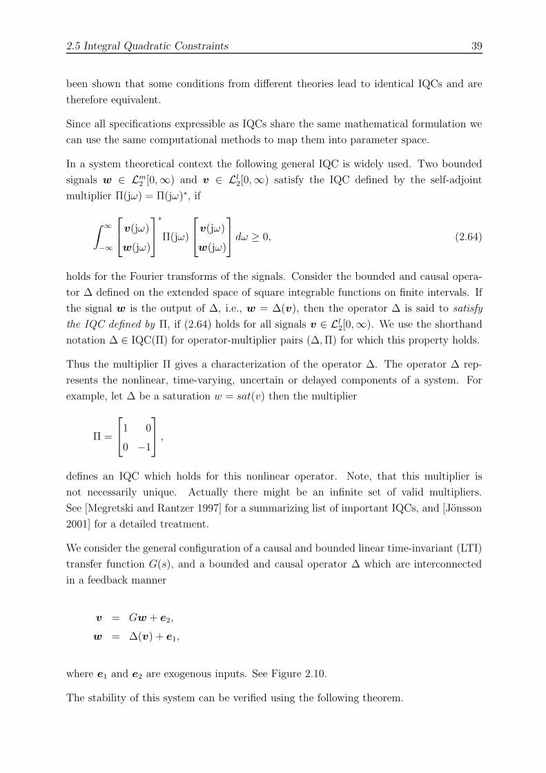
2.5 Integral Quadratic Constraints 39
been shown that some conditions from different theories lead to identical IQCs and are
therefore equivalent.
Since all specifications expressible as IQCs share the same mathematical formulation we
can use the same computational methods to map them into parameter space.
In a system theoretical context the following general IQC is widely used. Two bounded
signals w ∈ Lm2 [0,∞) and v ∈ Ll
2[0,∞) satisfy the IQC defined by the self-adjoint
multiplier Π(jω) = Π(jω)∗, if
∫ ∞
−∞
v(jω)
w(jω)
∗
Π(jω)
v(jω)
w(jω)
dω ≥ 0, (2.64)
holds for the Fourier transforms of the signals. Consider the bounded and causal opera-
tor ∆ defined on the extended space of square integrable functions on finite intervals. If
the signal w is the output of ∆, i.e., w = ∆(v), then the operator ∆ is said to satisfy
the IQC defined by Π, if (2.64) holds for all signals v ∈ Ll2[0,∞). We use the shorthand
notation ∆ ∈ IQC(Π) for operator-multiplier pairs (∆, Π) for which this property holds.
Thus the multiplier Π gives a characterization of the operator ∆. The operator ∆ rep-
resents the nonlinear, time-varying, uncertain or delayed components of a system. For
example, let ∆ be a saturation w = sat(v) then the multiplier
Π =
1 0
0 −1
,
defines an IQC which holds for this nonlinear operator. Note, that this multiplier is
not necessarily unique. Actually there might be an infinite set of valid multipliers.
See [Megretski and Rantzer 1997] for a summarizing list of important IQCs, and [Jonsson
2001] for a detailed treatment.
We consider the general configuration of a causal and bounded linear time-invariant (LTI)
transfer function G(s), and a bounded and causal operator ∆ which are interconnected
in a feedback manner
v = Gw + e2,
w = ∆(v) + e1,
where e1 and e2 are exogenous inputs. See Figure 2.10.
The stability of this system can be verified using the following theorem.

40 Control Specifications and Uncertainty
G
∆
we1
v e2
Figure 2.10: General IQC feedback structure
Theorem 2.9 [Megretski and Rantzer 1997]
Let G(s) ∈ RHl×m∞ , and let ∆ be a bounded causal operator. Assume that
(i) for τ ∈ [0; 1], the interconnection (G, τ∆) is well-posed,
(ii) for τ ∈ [0; 1], the IQC defined by Π is satisfied by τ∆,
(iii) there exists ε > 0 such that
G(jω)
I
∗
Π(jω)
G(jω)
I
≤ −εI, ∀ω ∈ R. (2.65)
Then, the feedback interconnection of G(s) and ∆ is stable.
�
Note that the considered feedback interconnection uses positive feedback only.
2.5.1 IQCs and Other Specifications
Many specifications presented in Section 2.4 can be cast as IQCs. In particular, we can
find a multiplier for all specifications which can be formulated as AREs. For example, for
the prominent condition that H∞ norm is less than one (small gain theorem), the IQC
multiplier is given by
Π =
I 0
0 −I
,
and
Π =
0 I
I 0
,
defines a valid multiplier for passivity.

2.5 Integral Quadratic Constraints 41
2.5.2 Mixed Uncertainties
For multiple, mixed uncertainties with different descriptions, e.g., LTI and time-varying,
the individual multipliers Πk can be combined into a single multiplier. The IQC can be
then used to verify stability with respect to both uncertainties occurring simultaneously.
A typical example for a system with mixed uncertainties is a system which has a satura-
tion actuator nonlinearity and where the plant is modeled using a multiplicative output
uncertainty.
Let a mixed uncertainty ∆ be given as,
∆ =
∆1 0
0 ∆2
, (2.66)
with associated IQC multipliers Π1 and Π2, which characterize the uncertainties ∆1
and ∆2. Then the overall IQC multiplier Π is given as the chess board like block (transfer)
matrix
Π =
Π1(1,1)0 Π1(1,2)
0
0 Π2(1,1)0 Π2(1,2)
Π∗1(1,2)
0 Π1(2,2)0
0 Π∗2(1,2)
0 Π2(2,2)
. (2.67)
2.5.3 Multiple IQCs
As mentioned previously, IQC multipliers are not unique. In fact, sometimes there are
not just IQCs with different parameters, but there are IQCs with fundamental differences.
In order to reduce the conservatism associated with the IQC uncertainty description, con-
vex parametrizations have been proposed [Jonsson 2001]. If ∆ ∈ IQC(Πk), k = 1, . . . , n,
then the convex combination of multipliers satisfies ∆ ∈ IQC(∑n
k=1 λkΠk), where λk ≥ 0.
In the PSA a dual and most times more practical approach is to utilize different IQCs by
iteratively mapping the individual IQCs. A good approximation of the uncertainty set,
e.g., using numerical LMI optimization, alleviates the increased conservativeness which
results from the reduced optimization variables used in the IQC stability test.

42 Mapping Equations
3 Mapping Equations
This chapter presents the mapping equations for control specifications considered in Chap-
ter 2. In particular we will present mapping equations based on algebraic Riccati and
Lyapunov equations. This approach is then extended in Section 3.4 to the uniform IQC
framework which allows to cover a large set of specifications and to broaden the system
classes and uncertainty descriptions.
Before we consider the new results for mapping additional specifications, we briefly present
some known results about eigenvalue based mapping equations.
3.1 Eigenvalue Mapping Equations
The roots of the parameter space approach stem from robust stability and have been
extended to eigenvalue specifications [Ackermann 1980]. A review of eigenvalue based
mapping equations is given in the following section.
Many important properties of control systems are characterized by eigenvalue specifica-
tions. This section briefly reviews the associated mapping equations. This serves two
purposes. First the mapping equations presented in this chapter will be compared to the
well-known equations for eigenvalue specifications. Second, as discussed in Section 2.4.7
and 2.4.9, some norm specifications lead to eigenvalue problems. Furthermore, it will be
shown that mapping several specifications considered in Section 2.4 involves a stability
condition, for example the H∞ norm. Generally, the PSA allows to separately map differ-
ent specifications. It seems to be always advantageous to map eigenvalue specifications,
especially since this can be done very efficiently. In that sense the results in this thesis
do not replace but extend the mapping of eigenvalue specifications.
Consider the characteristic polynomial pc(s) of a control system (SISO or MIMO). Math-
ematically pc(s) is calculated as the determinant of the matrix [sI − A], where A is the
closed loop system matrix, so that the roots of pc(s) coincide with the eigenvalues of A.
Without loss of generality, let the characteristic equation of a parametric system with n
states and coefficients ai be given as
pc(s, q) =
n∑
i=0
ai(q)si. (3.1)
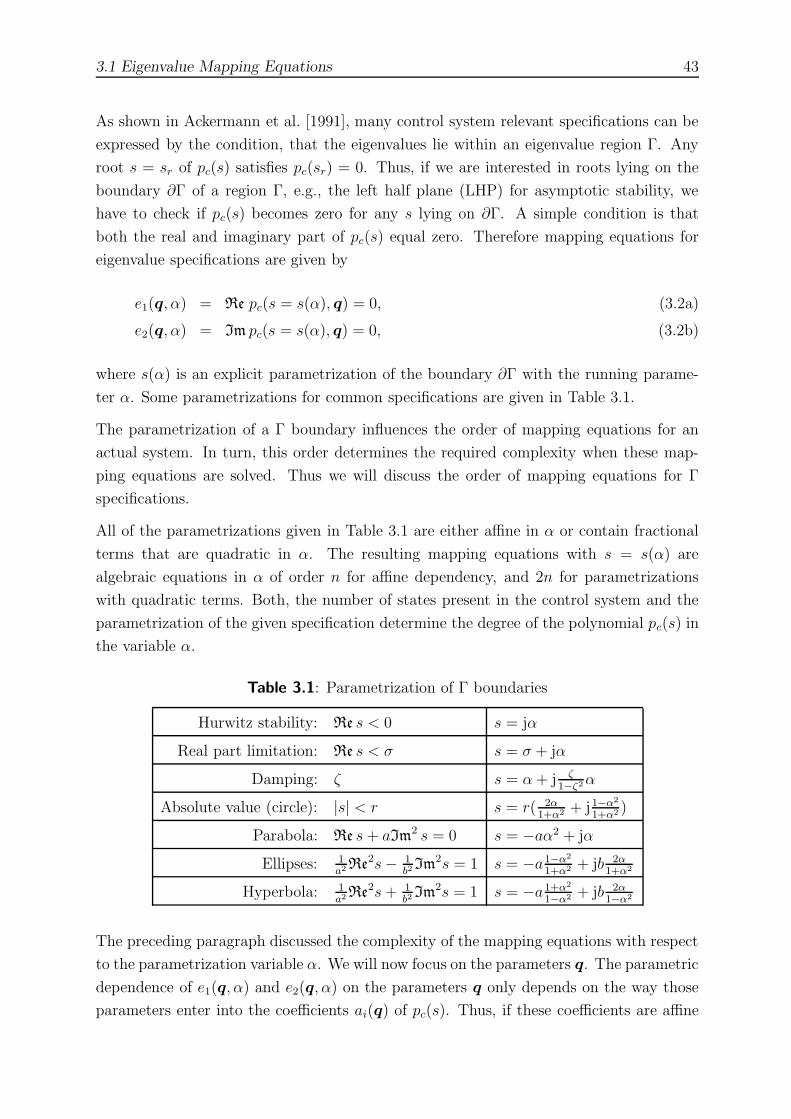
3.1 Eigenvalue Mapping Equations 43
As shown in Ackermann et al. [1991], many control system relevant specifications can be
expressed by the condition, that the eigenvalues lie within an eigenvalue region Γ. Any
root s = sr of pc(s) satisfies pc(sr) = 0. Thus, if we are interested in roots lying on the
boundary ∂Γ of a region Γ, e.g., the left half plane (LHP) for asymptotic stability, we
have to check if pc(s) becomes zero for any s lying on ∂Γ. A simple condition is that
both the real and imaginary part of pc(s) equal zero. Therefore mapping equations for
eigenvalue specifications are given by
e1(q, α) = Re pc(s = s(α), q) = 0, (3.2a)
e2(q, α) = Im pc(s = s(α), q) = 0, (3.2b)
where s(α) is an explicit parametrization of the boundary ∂Γ with the running parame-
ter α. Some parametrizations for common specifications are given in Table 3.1.
The parametrization of a Γ boundary influences the order of mapping equations for an
actual system. In turn, this order determines the required complexity when these map-
ping equations are solved. Thus we will discuss the order of mapping equations for Γ
specifications.
All of the parametrizations given in Table 3.1 are either affine in α or contain fractional
terms that are quadratic in α. The resulting mapping equations with s = s(α) are
algebraic equations in α of order n for affine dependency, and 2n for parametrizations
with quadratic terms. Both, the number of states present in the control system and the
parametrization of the given specification determine the degree of the polynomial pc(s) in
the variable α.
Table 3.1: Parametrization of Γ boundaries
Hurwitz stability: Re s < 0 s = jα
Real part limitation: Re s < σ s = σ + jα
Damping: ζ s = α + j ζ1−ζ2 α
Absolute value (circle): |s| < r s = r( 2α1+α2 + j1−α2
1+α2 )
Parabola: Re s + aIm2 s = 0 s = −aα2 + jα
Ellipses: 1a2 Re
2s − 1b2
Im2s = 1 s = −a 1−α2
1+α2 + jb 2α1+α2
Hyperbola: 1a2 Re
2s + 1b2
Im2s = 1 s = −a 1+α2
1−α2 + jb 2α1−α2
The preceding paragraph discussed the complexity of the mapping equations with respect
to the parametrization variable α. We will now focus on the parameters q. The parametric
dependence of e1(q, α) and e2(q, α) on the parameters q only depends on the way those
parameters enter into the coefficients ai(q) of pc(s). Thus, if these coefficients are affine

44 Mapping Equations
in q, the resulting mapping equations will be affine in q. This affine dependence is of great
impact, since for this case the mapping equations can be easily solved for two parameters.
For the synthesis of robust controllers the affine dependence of pc(s) on two controller
parameters can be enforced by choosing an appropriate controller structure for SISO sys-
tems. However, for MIMO systems additional conditions have to hold. If two parameters
are affinely present only in a single row or column of A, we cannot get any terms resulting
from products of parameters present in A, since pc(s) is calculated as det[sI − A]. For
MIMO systems with static-gain feedback, this is the case, if two parameters related to
the gains of the same input or output are considered.
The mapping equation (3.2) determines critical parameters for general complex eigenval-
ues s. The critical parameters obtained by (3.2) are thus called complex root bound-
ary (CRB). Furthermore two special cases exist. These are the so-called real root bound-
ary (RRB) and infinite root boundary (IRB). The first corresponds to roots being purely
real which can be mapped by using (3.2a) solely. The latter is characterized by roots
going through infinity. The characteristic polynomial pc(s) has a degree drop for an IRB,
i.e., one or more leading coefficients vanish. The RRB and IRB conditions will mathe-
matically reappear for MIMO specifications, although their interpretation is less intuitive
there.
The mathematical theory required for the mapping equations based on Riccati equations is
more involved. We will present the relevant properties in the next section. See Appendix A
for more details.
3.2 Algebraic Riccati Equations
This section gives an overview of algebraic Riccati equations (AREs). The general ARE
for the unknown matrix X is given by
XRX − XP − P ∗X − Q = 0 , (3.3)
where P , R, and Q are given quadratic complex matrices of dimension n with Q and R
Hermitian, i.e., Q = Q∗, R = R∗. Although in most applications in control theory P , R,
and Q will be real, the results will be given for complex matrices where possible.
An ARE is a matrix equation that is quadratic in an unknown Hermitian matrix X. It can
be seen as a matrix extension to the well-known scalar quadratic equation ax2 +bx+c = 0
that obviously has two, not necessarily real solutions.
An ARE has in general many solutions. Real symmetric solutions, and especially the
maximal solution, play a crucial role in the classical continuous time quadratic control

3.2 Algebraic Riccati Equations 45
problems [Kwakernaak and Sivan 1972]. Numerical algorithms for finding real symmetric
solutions of the ARE have been developed (see, e.g., [Laub 1979]). Many important
problems in dynamics and control of systems can be formulated as AREs [Boyd et al.
1994], [Zhou et al. 1996]. The importance of Riccati equations and the connection between
frequency domain inequalities, e.g., ||G(s)||∞ ≤ 1, has been pointed out by Willems [1971].
Later on it was shown, that the famous and long sought solution to the state-space H∞
problem can be found using AREs [Petersen 1987].
In general, the symbolic solution of AREs is not possible due to the rich solution struc-
ture. Despite that, a successive symbolic elimination of variables using Grobner bases is
considered in Forsman and Eriksson [1993]. Although this symbolic elimination might
reveal some insight into the structure and parameter dependency of the solution set, the
explicit solution is obtainable only for degenerate cases. The authors of the latter report
also conclude, that the computational complexity of the required symbolic computations
can be quite large.
For R = 0 the general ARE reduces to an affine matrix equation in X. These so-called
Lyapunov equations have proven to be very useful in analyzing stability and controllabil-
ity [Gajic and Qureshi 1995], while the design of control systems usually involves AREs.
Since an ARE is in general not explicitly solvable, there is no direct way to obtain map-
ping equations from AREs. These mapping equations will be derived using some special
properties of AREs.
Associated with the general ARE (3.3) is a 2n × 2n Hamiltonian matrix:
H :=
−P R
Q P ∗
. (3.4)
The matrix H in (3.4) can be used to obtain the solutions to the equation (3.3), see
Theorem A.1 for a constructive method. For the PSA these solutions are not relevant.
This is equivalent to the fact that the PSA does not compute actual eigenvalues when
mapping Γ specifications. Nevertheless we will use a particular property of (3.4). Namely
the set of all eigenvalues of H is symmetric about the imaginary axis. To see that,
introduce
J :=
0 −I
I 0
.
It follows that J−1HJ = −JHJ = −H∗. Thus H and −H∗ are similar and λ is an
eigenvalue of H if and only if −λ is.
The following well-known theorem [Zhou et al. 1996] provides an important link between
solutions of AREs and the Hamiltonian matrix H.

46 Mapping Equations
Theorem 3.1 Stabilizing solutions
Suppose that R ≥ 0, Q = Q∗, (P, R) is stabilizable, and there is a Hermitian
solution of (3.3). Then for the maximal Hermitian solution X+ of (3.3), P −RX+
is stable, if and only if the Hamiltonian matrix H from (3.4) has no eigenvalues on
the imaginary axis.
�
Note: A Hermitian solution X+ (resp. X−) of (3.3) is called maximal (resp. minimal)
if X− ≤ X ≤ X+ for all X satisfying (3.3), where X1 ≤ X2 means that X2 − X1 is
non-negative definite.
A proof of Theorem 3.1 is given in the Appendix in Section A.2. Theorem 3.1 shows that
the non-existence of pure imaginary eigenvalues is a necessary and sufficient condition
that the ARE (3.3) has a maximal, stabilizing, Hermitian solution. Since we have seen in
Chapter 2 that the adherence of many control specifications is equivalent to the existence
of a maximal, stabilizing, Hermitian solution of an ARE, we can test this adherence by
checking if the associated Hamiltonian matrix H has no pure imaginary eigenvalues.
The PSA deals with uncertain parameters q. The purpose of the next subsection is to
extend the previous results for invariant matrices to matrices with uncertain parameters.
3.2.1 Continuous and Analytic Dependence
So far we considered AREs with constant matrices. Suppose now that the matrices P, Q,
and R are analytic functions of a real parameter q ∈ R, i.e., P = P (q), Q = Q(q),
and R = R(q). We are thus concerned with the parametric ARE
X(q)R(q)X(q) − X(q)P (q) − P (q)∗X(q) − Q(q) = 0 , (3.5)
and associated Hamiltonian matrix H(q) defined analogously to (3.4).
Before we turn to the analytic dependence of maximal, stabilizing solutions and the
important equivalence of the eigenvalue properties of the Hamiltonian matrix H similar
to Theorem 3.1, we study the continuity of all maximal solutions of (3.5) with respect
to q.
If an ARE has Hermitian solutions, then there is a maximal Hermitian solution X+ for
which Λ(P −RX+) lies in the closed left half-plane. See Theorem A.2 for a rigorous state-
ment of this fact. The behavior of X+ as a function of P, Q, and R will be characterized
subsequently.

3.2 Algebraic Riccati Equations 47
Lemma 3.2 (Lancaster,Rodman)
The maximal Hermitian solution X+ of (3.5) is a continuous function of the ma-
trices (P, Q, R) ∈ Cn,n.
�
Although Lemma 3.2 is concerned with the continuity of maximal Hermitian solutions,
these solutions are in general not differentiable. That is, the maximal parametric solu-
tion X+ = X+(q) is not necessarily an analytic function of the real parameter q. The
analyticity of maximal Hermitian solutions is ensured by the invariance of the number of
pure imaginary eigenvalues of H.
The following theorem provides the link between control system specifications and the
Hamiltonian matrix H(q). This theorem forms the corner stone of ARE based mapping
equations. It appeared partly in a mathematical context in [Ran and Rodman 1988].
See [Lancaster and Rodman 1995] for a detailed exposition.
Theorem 3.3 (Lancaster,Rodman)
Let P = P (q), Q = Q(q), and R = R(q) be analytic, complex n×n matrix functions
of q on a real interval [q−; q+], with R(q) positive semidefinite Hermitian, Q(q)
Hermitian, and (P (q), R(q)) stabilizable for every q ∈ [q−; q+]. Assume that for
all q ∈ [q−; q+], the Riccati equation (3.5) has a Hermitian solution. Further assume
that the number of pure imaginary or zero eigenvalues of
H(q) :=
−P (q) R(q)
Q(q) P (q)∗
(3.6)
is constant. Then the maximal solution X+(q) of (3.5) is an analytic function of the
parameter q ∈ [q−; q+]. Conversely, if X+(q) is an analytic function of q ∈ [q−; q+],
then the number of pure imaginary or zero eigenvalues of H(q) is constant.
�
Proof:
The proof of this theorem is rather involved and provides no insight for the successful
application, i.e., the derivation of the mapping equations. It is therefore omitted
for brevity. See [Lancaster and Rodman 1995] for a sketch of the proof.
�

48 Mapping Equations
Theorem 3.3 is applicable to AREs, where the matrices P, Q and R are real. We get
necessarily real maximal solutions X+ for this control theory relevant case.
The previous results can be generalized to the case when P (q), Q(q) and R(q) are analytic
functions of several real variables q = (q1, . . . , qp) ∈ Q, where Q is an open connected set
in Rp.
3.3 Mapping Specifications into Parameter Space
In this section we present the mapping equations for the specifications given in Section 2.4
for systems with uncertain parameters.
For eigenvalue specifications the boundary of the desired region in the eigenvalue plane
is mapped into a parameter plane by the characteristic polynomial. Using the real and
imaginary part of the characteristic polynomial, two mapping equations are obtained
which depend on a generalized frequency α and the uncertain parameters q. The mapping
equations presented in this section will have a similar structure.
Actually, all mapping equations presented in this thesis will consist of pe individual equa-
tions with uncertain parameters q ∈ Rp and pe − 1 auxiliary variables. Usually pe is
either 1 or 2.
Thus if the vector of uncertain parameters q is of dimension p = 1, we get either a single
equation or a regular system of equations that can be solved for q. This allows to explicitly
determine the critical parameter values of q for which the specification is marginally ful-
filled. Related to this case is the dual problem of direct performance evaluation considered
in Section 3.8.
For p > 1 we get an underdetermined set of equations. The case p = 2 is not only
important for the easily visualized plots, but also because it admits tractable solution
algorithms considered in Chapter 4. For p > 2 gridding of p − 2 parameters is necessary
to determine the resulting solution sets.
3.3.1 ARE Based Mapping
While we provided the definition of H∞ norm, dissipativity and complex stability radius
specifications, we pointed out that all of these specifications are equivalent to the existence
of a maximal, Hermitian solution of an ARE. Using Theorem 3.1 we can in turn formulate
the adherence of the given specifications as the non-existence of pure imaginary eigenvalues
of an associated Hamiltonian matrix. This is a well-known fact used in standard numerical
algorithms [Boyd et al. 1989].

3.3 Mapping Specifications into Parameter Space 49
−3 −2 −1 0 1 2 3−2
−1.5
−1
−0.5
0
0.5
1
1.5
2
ℜ{λ}
ℑ{λ}
Figure 3.1: Appearance of pure imaginary eigenvalues
Consider now the uncertain parameter case. Using Theorem 3.3 we can extend this
equivalence to systems with analytic dependence on uncertain parameters. Given a spe-
cific parameter q∗ ∈ Rp for which a maximal, Hermitian solution X+(q∗) exists, we know
from Theorem 3.1 that the Hamiltonian matrix (3.6) has no pure imaginary eigenvalues.
Using Theorem 3.3 we can extend this property as long as the number of eigenvalues on
the imaginary axis is constant. In other words, having found a parameter for which a
specification described by an ARE holds, the same specification holds as long as the num-
ber of imaginary eigenvalues of the associated Hamiltonian matrix (3.6) is zero. Hence,
the boundary of the region for which the desired specification holds is formed by param-
eters for which the number of pure imaginary eigenvalues of (3.6) changes. A new pair
of imaginary eigenvalues of (3.6) arises, if either two complex eigenvalue pairs become
a double eigenvalue pair on the imaginary axis, or if a double real pair becomes a pure
imaginary pair. Note: Another possibility is a drop in the rank of H, which corresponds
to eigenvalues going through infinity. The appearance of pure imaginary eigenvalues is
depicted in Figure 3.1.
Let us first discuss the appearance of pure imaginary eigenvalues through a double pair
on the imaginary axis. The matrix H(q) has an eigenvalue at λ = jω if
det [jωI − H(q)] = 0. (3.7a)
In general a polynomial f(ω) has a double root not only if f(ω) = 0, but the derivative
of f(ω) with respect to the argument ω has to vanish also
∂f(ω)
∂ω= 0.

50 Mapping Equations
Since the characteristic polynomial of H(q) (3.7a) is a polynomial, we obtain
∂
∂ωdet [jωI − H(q)] = 0, (3.7b)
as the second condition for a double eigenvalue at λ = jω. Equations (3.7a) and (3.7b)
define two polynomial equations that can be used to map a given specification into pa-
rameter space.
A necessary condition for a real eigenvalue pair to become a pure imaginary pair through
parameter changes is
det [jωI − H(q)] ω=0 = det H(q) = 0. (3.8)
Additionally the opposite end of the imaginary axis has to be considered
det [jωI − H(q)] ω=∞. (3.9)
Equation (3.9) is just the coefficient of the term with the highest degree in ω of the
determinant det[jωI − H(q)].
Equation (3.8) is not sufficient, since it determines all parameters for which (3.6) has a
pair of eigenvalues at the origin. This includes real pairs that are just interchanging on
the real axis. To get sufficiency we have to check all parameters satisfying (3.8), if there
are only real eigenvalues. Figure 3.2 shows the two possible eigenvalue paths that are
determined by (3.8). The same check has to be performed for solutions of (3.9), because
here eigenvalues can interchange at infinity and (3.9) is not sufficient as well.
−3 −2 −1 0 1 2 3−2
−1.5
−1
−0.5
0
0.5
1
1.5
2
ℜ{λ}
ℑ{λ}
−3 −2 −1 0 1 2 3−2
−1.5
−1
−0.5
0
0.5
1
1.5
2
ℜ{λ}
ℑ{λ}
Figure 3.2: Possible eigenvalue paths for real root condition
From the eigenvalue spectrum of a Hamiltonian matrix follows that (3.7a) is purely real
and does not contain any imaginary terms. This fact is interesting in the following com-
parison and we will revisit this property in Section 3.5, where we evaluate the complexity
of the mapping equations.
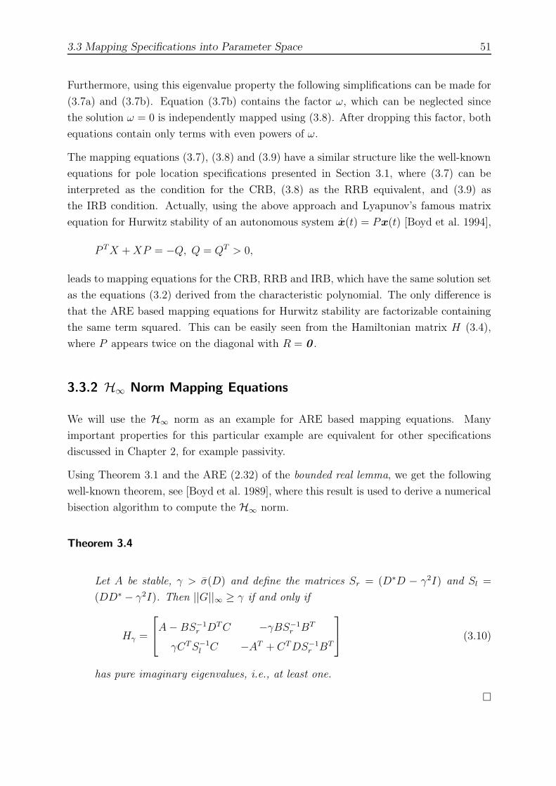
3.3 Mapping Specifications into Parameter Space 51
Furthermore, using this eigenvalue property the following simplifications can be made for
(3.7a) and (3.7b). Equation (3.7b) contains the factor ω, which can be neglected since
the solution ω = 0 is independently mapped using (3.8). After dropping this factor, both
equations contain only terms with even powers of ω.
The mapping equations (3.7), (3.8) and (3.9) have a similar structure like the well-known
equations for pole location specifications presented in Section 3.1, where (3.7) can be
interpreted as the condition for the CRB, (3.8) as the RRB equivalent, and (3.9) as
the IRB condition. Actually, using the above approach and Lyapunov’s famous matrix
equation for Hurwitz stability of an autonomous system x(t) = Px(t) [Boyd et al. 1994],
P TX + XP = −Q, Q = QT > 0,
leads to mapping equations for the CRB, RRB and IRB, which have the same solution set
as the equations (3.2) derived from the characteristic polynomial. The only difference is
that the ARE based mapping equations for Hurwitz stability are factorizable containing
the same term squared. This can be easily seen from the Hamiltonian matrix H (3.4),
where P appears twice on the diagonal with R = 0 .
3.3.2 H∞ Norm Mapping Equations
We will use the H∞ norm as an example for ARE based mapping equations. Many
important properties for this particular example are equivalent for other specifications
discussed in Chapter 2, for example passivity.
Using Theorem 3.1 and the ARE (2.32) of the bounded real lemma, we get the following
well-known theorem, see [Boyd et al. 1989], where this result is used to derive a numerical
bisection algorithm to compute the H∞ norm.
Theorem 3.4
Let A be stable, γ > σ(D) and define the matrices Sr = (D∗D − γ2I) and Sl =
(DD∗ − γ2I). Then ||G||∞ ≥ γ if and only if
Hγ =
A − BS−1
r DT C −γBS−1r BT
γCT S−1l C −AT + CT DS−1
r BT
(3.10)
has pure imaginary eigenvalues, i.e., at least one.
�

52 Mapping Equations
This theorem provides the Hamiltonian matrix needed in the general mapping equa-
tions (3.7), (3.8) and (3.9). In order to get the mapping equations, we have to compute
the determinant of the partitioned matrix det[jωI − H]. For a 2 × 2 block matrix
M =
M11 M12
M21 M22
the determinant is
det M = det M11 det[M22 − M21M
−111 M12
],
with M11 nonsingular. For ease of presentation let D = 0 , then det[jωI − Hγ] can be
written as
det [jωI − Hγ] = det [jωI − A] det[jωI + AT + γ2CT C(jωI − A)−1BBT
]. (3.11)
The first factor of the latter equation is just the Hurwitz stability condition. This is in line
with the fact that the H∞ norm requires the transfer function G(s) being stable. When
we directly compute det[jωI − Hγ] the stability related factor det[jωI − A] is canceled.
Hence, stability has to be mapped separately. Without this additional condition we
are actually mapping an L∞ norm condition. Concluding, apart from the H∞ norm
condition det[jωI − Hγ ], the Hurwitz stability condition has to be mapped additionally
using the mapping equations for Hurwitz stability described in Section 3.1.
The next point to notice about the H∞ norm mapping is that the static feedthrough
condition σ(D) < γ in Theorem 3.4 is implicitly mapped by (3.8) and (3.9). This can be
shown using a frequency domain formulation. See Section 3.7, which considers alternative
derivation of mapping equations for some specifications.
Note that the mapping equations for the H∞ norm are not just characterizing the pa-
rameters for which ||G||∞ = γ. Actually, all parameters for which G(s, q) has a singular
value σ(G) = γ are determined. Thus, we might get boundaries in the parameter space
for which the i-th biggest singular value σi has the specified value γ. This is similar to
eigenvalue specifications, where we get boundaries for each eigenvalue crossing of the Γ-
boundary. Analogously to the Γ-case, the resulting regions in the parameter space have
to be checked, if the specifications are fulfilled or violated (possibly multiple times).
If the critical gain condition on the static feedthrough matrix σ(D) = γ is fulfilled,
e.g., if D = γI, then Sl and Sr are singular. A remedy is to either consider a dif-
ferent performance level γ or to use a high-low frequency transformation and map the
condition ||G(s)||∞ = γ, where G(s) = G(s−1), since ||G||∞ = ||G||∞. A state-space
representation of G(s), which retains stability if A is stable, is given as
G(s) ∼=
A−1 −A−1B
CA−1 D − CA−1B
. (3.12)

3.3 Mapping Specifications into Parameter Space 53
To make the presented theory more clear we will consider a very simple exemplary system
in Example 3.2 on page 71.
3.3.3 Passivity Mapping Equations
The Hamiltonian matrix for dissipativity follows from the ARE (2.41) as
Hη =
A + BSC −BSB∗
C∗SC −(A + BSC)∗
, (3.13)
where S = (2ηI − D − D∗)−1. The specific mapping equations are then easily formed
using (3.7), (3.8), and (3.9).
In Section 2.4.2 the ARE for passivity was only valid for D 6= 0 . The following derivation
therefore relies on the more general dissipativity to obtain mapping equations for the not
uncommon case D = 0 .
For D = 0 , S reduces to S = 12η
I, and the Hamiltonian matrix Hη becomes
Hη =
A + 1
2ηBC − 1
2ηBB∗
12η
C∗C −(A + 12η
BC)∗
, (3.14)
The mapping equations for passivity can be obtained by evaluating the limit of the general
equations with H = Hη where η goes to zero, after extracting factors which only depend
on η. Since in general, det[jωI − Hη] is either fractionless with respect to η or a fraction
with denominator η, we get the relevant factor by simply evaluating the numerator.
More specifically the two mapping equations for the CRB condition are given as,
limη→0
num det [jωI − Hη] = 0, (3.15)
and
∂
∂ωlimη→0
num det [jωI − Hη] = 0. (3.16)
The RRB condition is given by
limη→0
num det Hη = 0, (3.17)
and the IRB follows as the leading coefficient of (3.15) with respect to ω
lcω limη→0
num det [jωI − Hη] = 0. (3.18)

54 Mapping Equations
For all four mapping equations (3.15)–(3.18) the limit has to be taken after the determi-
nant is calculated. A simple passivity example is presented in Example 5.6.
A dual approach to obtain mapping equations for passivity would be to use the results
from Section 2.4.3 and transform the passivity or positive realness condition into an H∞
norm problem.
Not surprisingly, we run into exactly the same singularity for D = 0 , which arises if we use
the passivity ARE (2.38) directly. Using Theorem 2.5 and the transformation (2.44) the
condition that G(s) = C(sI − A)−1B is positive real can be formulated as ||G(s)||∞ < 1,
where
G(s) ∼=
A − BC 2B
−C I
.
The resulting matrices Sr and Sl for the associated Hamiltonian matrix Hγ in Theorem 3.4
thus become zero.
3.3.4 Lyapunov Based Mapping
We now turn to special variants of AREs. If the quadratic term R of the general ARE (3.3)
vanishes, a so-called Lyapunov equation is obtained:
P ∗X + XP + Q = 0 , (3.19)
where Q = Q∗. Apply the Kronecker stacking operator (see Section A.1) to get
(P ∗ ⊕ P ) vec(X) = − vec(Q). (3.20)
This equation has a unique solution X if and only if λi(P ) + λj(P ) 6= 0, ∀ i, j.
In control theory, equation (3.19) is commonly used to test stability, controllability, and
observability. While stability is not of interest here, because it can be easily handled
by the classical PSA, Chapter 2 presented several specifications, e.g., the H2 norm, that
were formulated with observability and controllability Gramians Wobs and Wcon, and the
associated Lyapunov equations
A∗Wobs + WobsA + C∗C = 0 , (3.21a)
AWcon + WconA∗ + BB∗ = 0 . (3.21b)
We shall first consider the parametric solution of a Lyapunov equation. Equation (3.19)
is an affine equation in the unknown matrix elements xij of X = XT . Thus (3.19) consti-
tutes a system of 12n(n + 1) linear equations, where n is the dimension of the quadratic

3.3 Mapping Specifications into Parameter Space 55
matrix P ∈ Cn,n. This system can be readily solved for X(q) using a computer alge-
bra system for any parametric dependency of P (q) and Q(q). Note that the symmetry
of (3.19) should be used to minimize the computational effort, instead of using the full
system (3.20). In comparing (3.19) and (3.21), we see that the symbolic observability and
controllability Gramians Wobs(q) and Wcon(q) are obtained as the solution of a system
of 12n(n + 1) linear equations.
We will now present the mapping equation for the H2 norm. Using equation (2.56), a
specification on the H2 norm like ||G(s, q)||2 ≤ γ can be mapped into the parameter
space. In order to use (2.56) as a mapping equation, we need the parameter dependent
observability Gramian Wobs(q). This matrix can be obtained as described above.
Substituting this parametric solution Wobs(q) into (2.56), the parametric mapping equa-
tion is obtained as
||G(s)||22 = trace[B(q)T Wobs(q)B(q)
]= γ2, (3.22)
where γ2 specifies the desired performance level.
The dual output controllable formulation is given by
||G(s)||22 = trace [C(q)Wcon(q)C(q)] = γ2. (3.23)
Equation (3.22) is an implicit equation in the uncertain parameters q. Since the desired
or achievable performance level is not known a priori, it is recommended to vary γ and
determine the set of parameters P2,good for which ||G(s)||22 = γ2 holds for multiple values γ.
Also, a gray-tone or color coding of the different sets P2,good(γ) is useful. The visualization
of parameter space results will be considered in greater detail in Section 4.7.
The H2 norm mapping equation (3.22) is a single equation, that depends only on the
system parameters q. This is in line with the fact that the general definition of the H2
norm includes an integral over all frequencies. Thus there is no auxiliary variable α or
frequency ω in the mapping equations.
This fact makes (3.22) useful on its own, as opposed to being solely used for mapping H2
norm specifications into a parameter plane, especially to analyze and design control sys-
tems for more than two parameters. Furthermore (3.22) will be used to directly evalu-
ate H2 norms in Section 3.8.
If the parameters q enter in a polynomial fashion into A(q), B(q), C(q), the mapping
equation (3.22) is a polynomial equation. There may be some special cases, when (3.22)
is affine in one or more parameters, but in general this equation is polynomial in q, even
if A(q), B(q), and C(q) are affine in q.

56 Mapping Equations
In general there is no difference in using either (3.22) or (3.23). Nevertheless depending
on the complexity of B(q) and C(q) one or the other mapping equation might be easier
to solve in isolated cases.
3.3.5 Maximal Eigenvalue Based Mapping
We conclude this section with the remaining specifications presented in Chapter 2 for
which no mapping equations have been derived yet. Both the Hankel and the general-
ized H2 norm can be expressed as a function of a parametric matrix. These associated
matrices can be computed using the solution of parametric Lyapunov equations.
To get mapping equations for the Hankel and generalized H2 norms, we apply standard
results for mapping eigenvalue specifications. Namely a condition λmax(M) = γ, where M
is a non-negative matrix leads to the mapping equation
det [γI − M ] = 0.
Accordingly the condition dmax(M) = γ, M ≥ 0 leads to the system of mapping equations
mii = γ, i = 1, . . . , n.
3.4 IQC Parameter Space Mapping
Our goal is to use the unifying framework of IQCs to find mapping equations which allow
to incorporate an even larger set of specifications. We will show that mapping IQCs ex-
tends the parameter space beyond the ARE mapping equations presented in the previous
section.
Having found the mapping equations for general IQC specifications enables us to con-
sider specifications from the input-output theory, absolute stability theory and the robust
control field. Specifications from all these research fields can be used in conjunction
with the parameter space approach. Using the same mathematical formulation the same
computational methods can be used for these different specifications.
IQCs have been introduced in Chapter 2. A brief treatment of IQCs was given in Sec-
tion 2.5, where the basic stability condition (iii) of Theorem 2.9 is given as
G(jω)
I
∗
Π(jω)
G(jω)
I
≤ −εI, ∀ω ∈ R. (3.24)
In the current section we state the main result, the mapping equations for IQCs. We
will first consider fixed, frequency-independent multipliers. Section 3.4.4 will then show

3.4 IQC Parameter Space Mapping 57
how to map specifications based on IQCs with frequency-dependent multipliers Π(jω) into
parameter space. As an example a nonlinear system is analyzed in Section 3.4.4 using a
frequency-dependent multiplier.
For many uncertainties not just a single multiplier but sets of multipliers exist to char-
acterize the uncertainty structure. Often these sets can be described by parametrized
multipliers. We will show how to utilize these additional degrees of freedom in order
to minimize the conservativeness inherent in mapping only a single multiplier in Sec-
tion 3.4.5. An exemplary problem that utilizes LMI optimization is given in Example 3.1,
Section 3.4.5.
3.4.1 Uncertain Parameter Systems
Consider an uncertain LTI system G(s, q) ∈ RHl×m∞ interconnected to a bounded causal
operator ∆ as shown in Figure 2.10. The parameters q ∈ Rp are uncertain but constant
parameters with possibly known range. The operator ∆ might represent various types of
uncertainties, including constant uncertain parameters not contained in q. Let Π be a
constant multiplier that characterizes the uncertainty ∆ with partition
Π =
Π11 Π12
Π∗12 Π22
. (3.25)
Conditions (i) and (ii) of Theorem 2.9 are parameter-independent. Hence, the parameter-
dependent stability condition (3.24), which can be written as
G(jω)∗Π11G(jω) + Π22 + Π∗12G(jω) + G(jω)∗Π12 ≤ −εI, ∀ω ∈ R, (3.26)
has to be fulfilled by all parameters in Pgood.
The avenue to determine mapping equations will be the application of the Kalman-
Yakubovich-Popov (KYP) lemma. Previously known results on how to map specifications
expressible as AREs are then easily applied to IQC specifications.
3.4.2 Kalman-Yakubovich-Popov Lemma
In this section, the well known Kalman-Yakubovich-Popov (KYP) lemma is discussed.
The KYP lemma relates very different mathematical descriptions of control theoretical
properties to each other. In particular, it shows close connections between frequency-
dependent inequalities, AREs and LMIs. Nowadays a very popular application of the
KYP lemma is to derive LMIs for frequency domain inequalities, since efficient numerical
algorithms for the solution of LMI problems exist.

58 Mapping Equations
Theorem 3.5 (Kalman, Yakubovich, Popov)
Let (A, B) be a given pair of matrices that is stabilizable and A has no eigenvalues
on the imaginary axis. Then the following statements are equivalent.
(i) R > 0 and the ARE
Q + XA + AT X − (XB + S)R−1(XB + S)T = 0 (3.27)
has a stabilizing solution X = XT ,
(ii) the LMI with unknown X
XA + AT X XB
BT X 0
+
Q S
ST R
> 0 (3.28)
has a solution X = XT ,
(iii) for a spectral factorization the condition
(jωI − A)−1B
I
∗
Q S
ST R
(jωI − A)−1B
I
> 0 (3.29)
holds ∀ω ∈ [0;∞),
(iv) there is a solution to the general LQR problem
minu
J =
∫ ∞
0
(x(t)T Qx(t) + 2x(t)T Su(t) + u(t)T Ru(t)) dt (3.30)
with x(t) = Ax(t) + Bu(t), x(0) = x0 and limt→∞ x(t) = 0.
(v) R > 0 and the Hamiltonian matrix
H =
A − BR−1ST BR−1BT
Q − SR−1ST −AT + SR−1BT
(3.31)
has no eigenvalues on the imaginary axis.
Proof. See, for example, [Rantzer 1996] or [Willems 1971].
�
In order to apply the KYP lemma we will need the following remark.
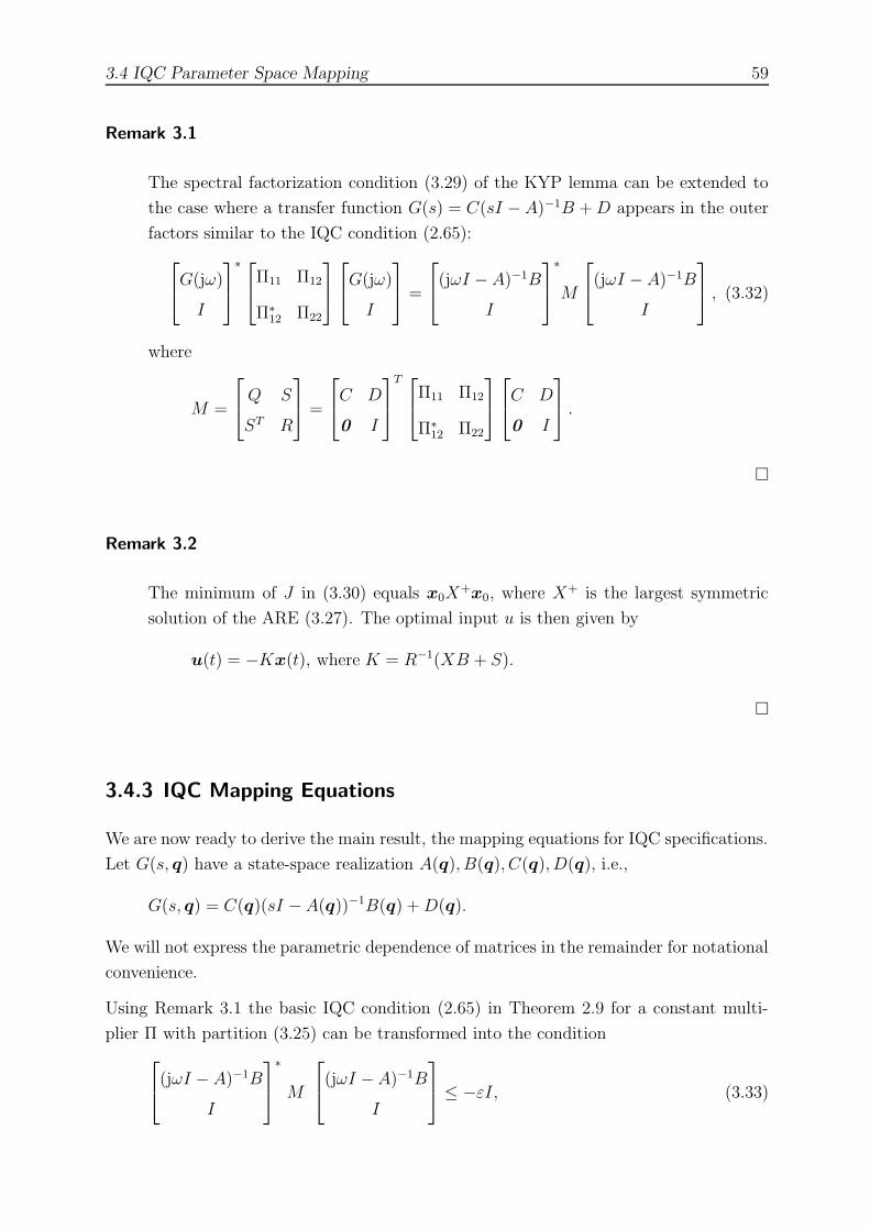
3.4 IQC Parameter Space Mapping 59
Remark 3.1
The spectral factorization condition (3.29) of the KYP lemma can be extended to
the case where a transfer function G(s) = C(sI − A)−1B + D appears in the outer
factors similar to the IQC condition (2.65):
G(jω)
I
∗
Π11 Π12
Π∗12 Π22
G(jω)
I
=
(jωI − A)−1B
I
∗
M
(jωI − A)−1B
I
, (3.32)
where
M =
Q S
ST R
=
C D
0 I
T
Π11 Π12
Π∗12 Π22
C D
0 I
.
�
Remark 3.2
The minimum of J in (3.30) equals x0X+x0, where X+ is the largest symmetric
solution of the ARE (3.27). The optimal input u is then given by
u(t) = −Kx(t), where K = R−1(XB + S).
�
3.4.3 IQC Mapping Equations
We are now ready to derive the main result, the mapping equations for IQC specifications.
Let G(s, q) have a state-space realization A(q), B(q), C(q), D(q), i.e.,
G(s, q) = C(q)(sI − A(q))−1B(q) + D(q).
We will not express the parametric dependence of matrices in the remainder for notational
convenience.
Using Remark 3.1 the basic IQC condition (2.65) in Theorem 2.9 for a constant multi-
plier Π with partition (3.25) can be transformed into the condition
(jωI − A)−1B
I
∗
M
(jωI − A)−1B
I
≤ −εI, (3.33)

60 Mapping Equations
where the multiplier is transformed into
M =
CT Π11C CT (Π12+Π11D)
(DT Π11+Π∗12)C DT Π11D+Π∗
12D+DT Π12+Π22
.
Since we are interested in mapping equations describing the boundaries of a parameter
set Pgood, we consider marginal satisfaction of (3.33), i.e., ε = 0.
Now, use statements (3.29) and (3.31) of the KYP lemma to get the equivalent condition
that the Hamiltonian matrix
H =
A 0
CT Π11C −AT
−
B
CT (Π12 + Π11D)
Π−122
CT (Π12 + Π11D)
−B
∗
, (3.34)
with Π22 = Π22 + DT Π12 + Π∗12D + DTΠ11D has no eigenvalues on the imaginary axis.
We have now formulated the adherence of a given IQC specification as the non-existence
of pure imaginary eigenvalues of an associated Hamiltonian matrix. Using Theorem 3.3
and the same arguments and methods as in Section 3.3.1, we can substitute (3.34) into
the ARE based mapping equations (3.7a), (3.8) and (3.9) to get mapping equations for
IQC based specifications. Thus the KYP lemma established the important relationship
which allows to derive mapping equations for IQC conditions. The consequence is that
the statements about the properties of ARE based mapping equations can be directly
transferred to the IQC mapping equations, e.g., the non-sufficiency of (3.8).
We extend the previous IQC results by considering frequency-dependent multipliers in
the next section.
3.4.4 Frequency-Dependent Multipliers
Consider the case when the multiplier Π is frequency-dependent, i.e., Π = Π(jω).
The common frequency domain criterion used in conjunction with IQCs for frequency-
dependent multipliers is
G(jω)
I
∗
Π(jω)
G(jω)
I
< 0, ∀ω ∈ [0;∞), (3.35)
where G(jω) ∈ RHl×m∞ and Π(jω) ∈ RHl+m×l+m
∞ .
A particular example of a frequency-dependent multiplier is the strong result by Zames
and Falb [1968] for SISO nonlinearities1. Put into the IQC framework, an odd nonlinear
1The results in [Zames and Falb 1968] can be only applied to MIMO nonlinearities using additional
restrictions, see [Safonov and Kulkarni 2000].

3.4 IQC Parameter Space Mapping 61
operator, e.g., saturation, satisfies the IQC defined by
Π(jω) =
0 1 + L(jω)
1 + L(jω)∗ −2 − L(jω) − L(jω)∗
,
where L(s) has an impulse response with L1 norm less than one.
Following [Megretski and Rantzer 1997], any bounded rational multiplier Π(jω) can be
factorized as
Π(jω) = Ψ(jω)∗ΠsΨ(jω), (3.36)
where Ψ(jω) absorbs all dynamics of Π(jω) and Πs is a static matrix. Actually factor-
ization (3.36) is known as a J-spectral factorization, which plays an important role on
its own in H∞ and H2 control theory [Green et al. 1990], or as a canonical Wiener-Hopf
factorization in operator theory [Bart et al. 1986].
We will now derive mapping equations for frequency-dependent multipliers by simple
transformations and equivalence relations. Rewrite (3.36) as
Π(jω) =
Ψ(jω)
I
∗
Πs 0
0 0
Ψ(jω)
I
, (3.37)
and apply a transformation similar to Remark 3.1, where Ψ(jω) has state-space represen-
tation Ψ(jω) = Cπ(jωI − Aπ)−1Bπ + Dπ to get
Π(jω) =
(jωI − Aπ)−1Bπ
I
∗
CT
π ΠsCπ CTπ ΠsDπ
DTπ ΠsCπ DT
π ΠsDπ
︸ ︷︷ ︸
Mπ
(jωI − Aπ)−1Bπ
I
. (3.38)
Next, partition the input matrix Bπ of Ψ(jω) according to the signals in the general IQC
feedback loop (see Figure 2.10) as Bπ = [Bπ,v Bπ,w], which was suggested in the deriva-
tion of a linear quadratic optimal control formulation of (3.35) in [Jonsson 2001], and
use (3.38) to write condition (3.35) as
(jωI − Aπ)−1(Bπ,vG(jω) + Bπ,w)
G(jω)
I
∗
Mπ
(jωI − Aπ)−1(Bπ,vG(jω) + Bπ,w)
G(jω)
I
< 0, (3.39)
for all ω ∈ [0;∞).

62 Mapping Equations
Let G(jω) = C(jωI − A)−1B + D, then the following state-space representation for the
factor to the right of Mπ in (3.39) can be deduced:
(jωI − Aπ)−1(Bπ,vG(jω) + Bπ,w)
G(jω)
I
=
Aπ Bπ,vC Bπ,vD + Bπ,w
0 A B
I 0 0
0 C D
0 0 I
(3.40)
=
A B
C D
. (3.41)
Using this state-space representation, condition (3.39) becomes
(C(jωI − A)−1B + D)∗Mπ(C(jωI − A)−1B + D) < 0, ∀ω ∈ [0;∞), (3.42)
or
(jωI − A)−1B
I
∗
CT
DT
Mπ
[
C D]
︸ ︷︷ ︸
M
(jωI − A)−1B
I
< 0, ∀ω ∈ [0;∞). (3.43)
As a result, we have obtained an IQC condition with a frequency-independent multi-
plier M , where
M =
CT
DT
Mπ
[
C D]
=
Q S
ST R
, (3.44)
and where (A, B) represents an augmented system composed of both the LTI system
dynamics and the multiplier dynamics. The multiplier matrices can be computed as,
Q =
CT
π ΠsCπ CTπ ΠsDπ,vC
CT DTπ,vΠsCπ CT DT
π,vΠsDΠ,vC
, (3.45)
S =
CT
π Πs(Dπ,vD + Dπ,w)
CT DTπ,vΠs(Dπ,vD + Dπ,w)
, (3.46)
R =[
(Dπ,vD + Dπ,w)T Πs(Dπ,vD + Dπ,w)]
. (3.47)
As in the frequency-independent case discussed in the previous section, we can now apply
the KYP lemma in order to obtain the Hamiltonian matrix which will lead to the map-
ping equations. Namely, use statements (3.29) and (3.31) of the KYP lemma to get the

3.4 IQC Parameter Space Mapping 63
equivalent condition that the Hamiltonian matrix
H =
A − BR−1ST BR−1BT
Q − SR−1ST −AT + SR−1BT
(3.48)
has no eigenvalues on the imaginary axis.
Hence frequency-dependent bounded rational multipliers Π(jω) can be mapped into pa-
rameter space using basic matrix transformations and the results from the previous sec-
tion.
3.4.5 LMI Optimization
For a system with fixed parameters, all multipliers considered so far led to a simple
stability test, which could be evaluated by computing the eigenvalues of a Hamiltonian
matrix (3.31). For systems with uncertain parameters q ∈ Rp, we showed how to map
an IQC specification into a parameter plane. But in general, the uniqueness of a multiplier
is not given.
While the main idea behind the IQC framework is to find a suitable multiplier for an
uncertainty, for many uncertainties a set of possible multipliers exists. Especially for
nonlinearities and time-delay systems there is an enormous list of publications involving
different multipliers. See [Megretski and Rantzer 1997] for some references. Depending on
the considered LTI system one or the other multiplier might be advantageous and yield
less conservative results.
For example, consider the following multiplier from [Jonsson 1999] for a system
x(t) = (A + U∆V )x(t), (3.49)
with slowly time-varying uncertainty ∆ and known rate bounds
Π(jω) =
Z Y T − jωW T
Y + jωW −X
. (3.50)
Jonsson [1999] derives a set of LMI conditions to check stability involving real matri-
ces W, X = XT , Y and Z = ZT . These matrices can be easily obtained solving a convex
optimization problem. The result of the optimization is not only a binary stability check,
but also an optimal multiplier Π(jω).
There are two different possibilities to exploit the degrees of freedom in the multiplier
formulation during the mapping process.

64 Mapping Equations
One approach would be to use a limited set of parameter points (q1, q2) for which we
obtain optimal multipliers and subsequently determine the set of good parameters Pgood
for each individual multiplier. The actual overall set of uncertain parameters which fulfill
the specification is then given as the union of all individual good sets.
The second approach could be denoted as adaptive multiplier mapping. Hereby we ob-
tain successive multipliers as we actually determine the boundary by moving along the
boundary of the set Pgood. Thus we adaptively correct the optimal multiplier on the way
as we generate the boundary by solving an underlying optimization problem.
While the first approach needs to solve a limited and predefined number of optimization
problems, the adaptive multiplier mapping requires a possibly large number of optimiza-
tion, which is not known a priori. Nevertheless the second approach gives the actual
set Pgood directly and there is no need to determine the union of individual sets. Fur-
thermore, when the actual mapping is expensive, it might be favorable to use a single
adaptive mapping run.
Example 3.1 The following example shows how the IQC results of the current section
can be used to extend the parameter space approach to stability checks with respect to
varying parameters.
Consider the following parametric system, which fits into the setup of problem (3.49),
x(t) =
q1 + q2 1 + q2
−3 −12− q1
+
0 2
5
25
0
∆
x(t), (3.51)
where ∆ is a diagonal matrix containing an arbitrarily fast varying parameter δ. The
parameter δ is assumed to be bounded in the interval [0; 1].
Note that if we treat δ as a constant parameter, then the set of good parameters is given
by δ = 0 since all stability sets for δ > 0 contain the set for δ = 0. So from the perspective
of constant parameters we do not lose anything, if we allow δ to deviate from δ = 0 to
values in the interval [0; 1].
We assume arbitrary fast variations of the parameter δ, therefore the matrix W , which
appears in (3.50), equals zero. Following [Jonsson 1999], system (3.49) is stable with
respect to ∆, if a feasible solution for the following LMI problem exists.

3.4 IQC Parameter Space Mapping 65
−3 −2 −1 0 1 2−3
−2
−1
0
1
2
q1
q2
Figure 3.3: Stability regions using adaptive LMI optimization
Find X = XT , Y, Z = ZT , P = P T such that,
X ≥ 0, (3.52)
AT P + PA + V T ZV PU + V T Y T
UT P + Y V −X
< 0, (3.53)
Z > 0, (3.54)
Z + Y + Y T − X > 0. (3.55)
We determine the stability boundaries in the q1, q2 parameter plane. In the first step we
calculate the maximal stability boundary using adaptive multiplier mapping. In each step
optimal values for the X, Y, and Z matrices, which determine the multiplier (3.50), are
computed. The resulting stability boundaries are shown in Figure 3.3 as a solid curve.
The figure also shows the common real root boundary, assuming uncertain, but constant δ
values, as a dotted line, and the complex root boundaries for δ = 0, and δ = 1 as dashed
lines.
Figure 3.4 shows the stability regions depicted as solid curves, which are obtained using
optimal multipliers for the points (0, 0), (1, 0), and (−1,−0.5). For comparison the
stability region obtained using adaptive multiplier mapping is shown as a dash-dotted

66 Mapping Equations
−3 −2 −1 0 1 2−3
−2
−1
0
1
2
q1
q2
Figure 3.4: Stability regions using multiple fixed IQC multipliers
curve. The figure shows that a small number of reference points might suffice to get a
rather accurate approximation of the true stability region. It should be noted that the LMI
problem (3.52) is only a feasible problem. Although the resulting multiplier guarantees
stability for the reference point, i.e. A(q1, q2), the resulting size of the stability region in
the (q1, q2) parameter plane is not necessarily maximal. Thus treating the parameters q1
and q2 as additional uncertainty to the ∆ uncertainty and augmenting the LMI problem
might lead to even larger stability regions.
For q1 = 0 and q2 > 0 the true stability limit is q2 = 0.23018, and instability occurs
near the origin for a switching behavior of δ. Whereas the optimal multiplier yields a
guaranteed stability for q2 = 0.067, which exemplifies the conservativeness of this IQC
condition. Nevertheless Figure 3.3 and Figure 3.4 show that the IQC condition gives
very accurate results for stability regions, where the varying parameter does not affect
the stability region. And the simplicity of the used multiplier (frequency-independent)
suggests that a more complicated multiplier might even improve the shown results. �
3.5 Complexity 67
3.5 Complexity
This section discusses the complexity of the mapping equations derived above. In par-
ticular we will look at the order of the equations as a function of the number of states
in the system and as a function of the input and output dimensions. Furthermore the
complexity with respect to the uncertain parameters q is considered.
3.5.1 ARE Mapping Equations
The complexity of ARE based mapping equations is determined by the Hamiltonian ma-
trix H defined in (3.4). The corresponding Hamiltonian matrix for all ARE expressible
specifications in this thesis, i.e., H∞ norm (2.32), passivity (2.38), dissipativity (2.41), cir-
cle criterion (2.48), Popov criterion (2.51) and complex structured stability radius (2.54),
can be written in the following form:
H =
A + BS1C −BS2B
T
CT S3C −(A + BS1C)T
, (3.56)
where Si, i = 1, . . . , 3, are specification dependent, nonsingular matrices, which depend
on D. For uncertain parameters q in the plant description, all matrices A, B, C and Si
can be parameter dependent.
The dimension of H depends only on the size of A ∈ Rn,n, where n equals the number
of states in the system, H ∈ R2n, 2n. The dimension of H does not increase with the
number of inputs and outputs. Thus complexity does not increase when we consider
MIMO instead of SISO systems.
The order of det[jωI −H] with respect to ω is 2n and corresponds directly to the number
of states. Note that (3.7a) has only terms with even powers of ω. Thus after we eliminate
the factor ω, the second, double root condition (3.7b) has order 2(n − 1) with respect
to ω.
The order of the mapping equations with respect to a single parameter q or qi can be
determined by studying a general determinant. The determinant of an arbitrary ma-
trix M ∈ Rn,n can be calculated as the algebraic sum of all signed elementary products
from the matrix. An elementary product is given by multiplying n entries of an n × n
matrix, all of which are from different rows and different columns:
det M =∑
π∈Sπ
sgn(π)m1π1m2π2 · · ·mnπn, (3.57)
where the index π in the above sum varies over all possible permutations Sπ of {1, . . . , n}.The total number of possible permutations is n!, which therefore equals the number of
terms in the defining sum of determinant.

68 Mapping Equations
For n = 3 the position of the individual factors for the 3! elementary products is shown
below:
∗∗
∗
∗∗
∗
∗∗
∗
∗∗
∗
∗∗
∗
∗∗
∗
.
The matrix A appears twice on the diagonal of H. Because an entry aij appears both at hij
and hn+j,n+i, there is always an elementary product that contains both hij and hn+j,n+i.
Thus the general determinant det[jωI − H], depends quadratically on the entries of A.
Hence, even if the entries of A depend affinely on qi we will get quadratic mapping equa-
tions in qi. This holds for special canonical representations, which yield a characteristic
polynomial with affine parameter dependency. The quadratic dependency of the map-
ping equations makes it clear that, even for really simple parameter dependence, we have
to deal with mapping equations that are more complicated than the mapping equations
obtained for eigenvalue specifications.
For parametric entries of the input and output matrices B and C it is obvious that we
get quadratic terms for each entry, since the Hamiltonian matrix H already has quadratic
terms due to BS2BT and CTS3C.
The appearance of entries from the D matrix in the final mapping equations depends
on the considered specification. Thus, there is no obvious way to show the dependence
of the mapping equations with respect to parameters in D. Nevertheless, evaluating the
dependence for each specification expressible as an ARE or by looking at the general IQC
Hamiltonian matrix (3.34), with Π22 = Π22 + DT Π12 + Π∗12D + DT Π11D, we can deduce
that entries of D will reappear as quadratic terms in the mapping equations.
3.5.2 Lyapunov Mapping Equations
Lyapunov based mapping equations can be obtained by evaluating one of the two equa-
tions given in (3.21). In order to determine the mapping equations we first have to solve
a system of linear equations, where the parametric coefficient matrix has size 12n(n + 1),
where n is the number of states of the considered transfer matrix. The resulting Gramian
has the same dimensions as A.
In the final step, we have to compute a parametric matrix product including the just
obtained Gramian, and determine the trace. Thus the main obstacle to compute Lyapunov
mapping equations is the symbolic solution of a linear system.
3.6 Further Specifications 69
3.5.3 IQC Mapping Equations
The order of the IQC mapping Hamiltonian matrix is given by the number of plant states
plus the number of states required to realize the multiplier. Thus, only for frequency-
dependent multipliers there is a multiplier state-space augmentation, and the complexity
increases. Hence, the accuracy gained by using a higher order multiplier has to be paid
for by an increased Hamiltonian matrix complexity and therefore increased computational
requirements.
3.6 Further Specifications
So far we covered a list of specifications that includes almost the entire list of specifi-
cations commonly used in control engineering. Nevertheless some candidates of unequal
importance are missing: the structured stability radius µ, the entropy, and the L1 norm.
The structured stability radius µ has been introduced to cope with parametric uncer-
tainties in the H∞ norm framework. To date there are only approximate methods to
estimate its value. So, there is no way to map µ specifications into a parameter space.
Since the structured stability radius tries to deal with mixed uncertainties it considers a
similar problem as the methods presented in this thesis. Having the definition of µ in
mind, we do not expect advantageous insights of mapping a specification for parametric
uncertainties into a parameter plane.
Another specification considered in the control literature is the entropy of a system. This
entity is actually not a norm, but it is closely related to the H2 and H∞ norm.
The γ-entropy [Mustafa and Glover 1990] of a transfer matrix G(s) is defined as
Iγ(G) :=
−γ2
2π
∫ ∞
−∞
ln det[I − γ2G(jω)G(jω)∗
]dω, if ||G||∞ < γ,
∞, otherwise.
(3.58)
The γ-entropy has been used as a performance index in the context of so-called risk
sensitive LQG stochastic control problems, and reappeared in the H∞ norm framework
in [Doyle et al. 1989] as the so-called central controller, where the selected controller
satisfying an H∞ norm condition minimizes the γ-entropy.
The γ-entropy of G(s), when it is finite, is given by
Iγ(G) = trace [BT XB], (3.59)
where X is the positive definite solution of the ARE
AT X + XA + CT C +1
γ2XBBT X = 0 . (3.60)

70 Mapping Equations
Although the familiar ARE might suggest that mapping equations for this specifications
can be derived, this is not the case. The existence of a solution to (3.60) can be tested with
the familiar Hamiltonian matrix (3.6). But in order to compute and map Iγ we actually
need this solution. Therefore the entropy does not fit into the presented framework and
no algebraic mapping equations can be derived.
Another example of a specification, that cannot be easily mapped, is the L1 or peak gain
norm:
||G(s)||1 := sup||w||∞ 6=0
||Gw||∞||w||∞
. (3.61)
For a given system, the total variation of the step response is the peak gain of its transfer
function, see [Lunze 1988]. This specification is not computable by algebraic equations.
Boyd and Barratt [1991] suggest to use numerical integration to calculate it. A remedy
might be to use lower and upper bounds given in [Boyd and Barratt 1991], and map H∞
and Hankel norm specifications. Namely, if G(s) has n poles, then the L1 norm can be
bounded by the Hankel and H∞ norm:
||G||∞ ≤ ||G||1 ≤ (2n + 1)||G||hankel ≤ (2n + 1)||G||∞. (3.62)
3.7 Comparison and Alternative Derivations
A particular strength of the approach pursued in this thesis is the generality. All spec-
ifications expressible as an ARE or Lyapunov equation can be considered. Nevertheless
there are alternative derivations of mapping equations for some specifications.
Most authors to date have considered either eigenvalue or frequency domain specifications
for SISO systems [Besson and Shenton 1999, Bunte 2000, Hara et al. 1991, Odenthal
and Blue 2000]. Reasons for this might be the elegant derivation of eigenvalue mapping
equations, which are computationally very attractive for practically relevant problems.
For frequency domain specifications the extension to MIMO systems is nontrivial and the
complexity associated with SISO mapping equations might have hindered the application
to MIMO systems.
3.8 Direct Performance Evaluation
The PSA maps specifications into a parameter plane. We are neither interested in the
direct, numerical evaluation of a specification, e.g., ||G(s, q∗)||∞, where q∗ is a fixed pa-
rameter vector, nor in the solution of an optimal control problem traditionally considered

3.8 Direct Performance Evaluation 71
in the H2 and H∞ literature. Nevertheless the presented mapping equations can be used
for the direct performance evaluation for some of the presented specifications.
Although in a different mathematical framework, Schmid [1993] devoted a large portion
of his work to the direct evaluation of the H∞ norm, see also [Kabamba and Boyd 1988].
The mapping equations establish conditions, that allow the direct computation of the H∞
norm. Thus, instead of using the numerically attractive bisection algorithm widely used
in control software, the H∞ norm can be computed by solving the two algebraic equa-
tions (3.7a) and (3.7b) in the two unknowns ω and γ. These positive solutions provide
candidate values γ for the H∞ norm. Additionally, the solutions of (3.8) and (3.9) are
computed and the H∞ norm of the system is given by the maximal value over all candi-
date solutions. As a byproduct, we get the frequency ω, for which the maximal singular
value occurs.
For the H2 norm the direct evaluation is simply possible by solving the linear equa-
tion (3.21b) and substituting the solution into the mapping equation (3.22).
Example 3.2 We use the mapping equations to directly compute the H∞ norm for the
open-loop transfer function
G(s) =1
(s + 1)(s + 2)
2 −2s
s 3s + 2
. (3.63)
A state-space representation for G(s) is given by
G(s) ∼=
−2 0
0 −1
1 2
1 1
−2 2
2 −1
0 0
0 0
. (3.64)
The mapping equations (3.7a) and (3.7b) become
e1 = γ4ω4 + (5γ4 − 14γ2)ω2 + 4γ4 − 8γ2 + 4,
e2 = ω(4γ4ω2 + 10γ4 − 28γ2).
This polynomial system of equations has only one single relevant solution ω = 1, γ =√
2
with ω, γ > 0.
The DC-gain condition (3.8) is
det Hγ = γ4 − 2γ2 + 1,

72 Mapping Equations
which has the positive solution γ = 1. Note that this can be easily observed by the fact
that G(j0) = I, and thus the singular values are given by σ1 = σ2 = 1.
There is no solution for (3.9) and we can conclude that the maximal singular value of G(s)
is given for ω = 1 and ||G(s)||∞ =√
2. �
3.9 Summary
The main contribution of this chapter is the presentation of a uniform framework that
allows to derive mapping equations for parametric control system specifications expressible
by AREs.
Besides ARE expressible specifications, previously unknown mapping equations for IQC
based stability tests are determined. Using the results in this section we can draw from the
vast number of available IQCs and incorporate them into the parameter space approach.
Furthermore, application of standard parameter space methods allows to include an even
larger list of specifications into control system analysis and design.
The resulting equations are similar to well-known Γ-stability mapping equations. This
allows similar computational methods for the mapping, although the complexity is in
general higher, due to the quadratic nature of the specifications.

73
4 Algorithms and Visualization
The purpose of computing is insight, not numbers.
Richard Hamming
The main contribution of this chapter is the presentation of algorithms which solve the
mapping problem, i.e., they plot the critical parameters in a parameter plane. Thus these
algorithms are a prerequisite to the successful application of the presented MIMO control
specifications in the parameter space context.
Geometrically, the mapping is either a curve plotting or surface-surface intersection prob-
lem. These can be approached with a variety of different techniques, including numerical,
analytic, geometric, and algebraic methods, and using various methods such as subdivi-
sion, tracing, and discretization. While classic algorithms used a single method, recently
algorithms which combine multiple methods or so-called hybrid algorithms appeared.
We will follow this line and combine previous known results such that the new combination
of basic building blocks forms an efficient algorithm for the mapping problem.
The robustness of the algorithm has to be considered. It is easy to generate a specialized,
fast algorithm for special curve intersections. This is actually the topic of solid geom-
etry, vision or computer-aided design, where the complexity of the geometrical objects
considered is known beforehand.
For practical experimentation the algorithms were implemented using Maple and Mat-
lab.
The Lyapunov based mapping equations in Section 3.3.4, e.g., for the H2 norm, directly
lead to an implicit polynomial equation
f(x, y) =
n∑
i,j=0
aijxiyj = 0, (4.1)
where x and y represent the two parameters of the parameter plane. In order to plot the
parameters, which satisfy a control system specification, we have to determine the curve Cof real solutions satisfying (4.1). General properties of algebraic curves will be presented
in Section 4.2.

74 Algorithms and Visualization
For ARE based mapping equations we get two polynomial equations
f1(x, y, ω) = 0,
f2(x, y, ω) = 0,(4.2)
and we are interested in the plane curve of real solutions (x, y) ∈ R2 which can be
obtained for all positive ω. Mathematically (4.2) defines a spatial curve in R3. Thus we
are interested in the plane curve C given as the projection of the spatial curve (4.2) onto
the plane ω = 0. Since (4.2) is a generalization of (4.1) we will first treat plane parameter
curves, and consider the extension to (4.2) in Section 4.5.
4.1 Aspects of Symbolic Computations
This section considers general aspects of symbolic computation and compares them to nu-
merical computations. This gives rationals for designing hybrid algorithms which employ
both symbolic and numerical computations, such that the overall results are obtained fast
and robust.
Symbolic computation is considerably different from numerics, as new aspects such as
internal data representation, memory usage, and coefficient growth arise, while difficult
aspects of numerical algorithms, e.g., rounding errors and numerical instability, disap-
pear [Beckermann and Labahn 2000]. The main advantage of symbolic computations is
the fact that general equations with unknown variables can be solved. Furthermore the
exact arithmetic avoids common problems of numerical algorithms introduced by finite
precision.
A common symbolic algebra package such as Maple can handle 216−1 individual symbolic
expressions. Compare this to the determinant of a matrix A with unknown entries aij.
The determinant of a matrix with size n has n! expressions. Thus even the modest size
of n = 9 exceeds the capacities of available software. And since the factorial grows much
faster than polynomial, even with more memory and computer power, the memory usage
will be always a limiting factor in the application of symbolic algorithms to real world
problems.
These limitations impose some restrictions on the application of the presented control
specifications. Although the mapping equations given in Chapter 3 can be computed
symbolically, treating all parameters as variable complicates the computations drastically.
A remedy is to substitute all parameters not part of the parameter plane into which the
specifications are mapped with their numerical values. For example, when we are mapping
the H2 norm specification into a q1, q2 parameter plane, all remaining parameters in the
state space model should be replaced by their numerical values prior to the mapping

4.2 Algebraic Curves 75
equation computation. Thus, if we are gridding a parameter q3, we will generate the
mapping equations for each grid point. This is much more attractive than computing
universal mapping equations, where q3 appears as a free parameter.
The computational complexity of symbolic algorithms cannot be measured by operational
complexity. The main reason is the varying cost associated with operations such as
addition or multiplication. The cost here depends on the size of the components and the
size of the result. This is related to the way computer algebra systems such as Maple
store expressions. Here all expressions are stored in an expression tree or more precise a
direct acyclic graph. The following example shows the possible explosion on the number
of expressions for a very small problem:
p1(s) = s2 + q1s + q2,
p2(s) = s2 + (q1 − q2)s + q1,
p1(s)p2(s) = s4 + (2q1 − q2)s3 + (q2
1 − q1q2 + q1 + q2)s2 + (q2
1 − q22 + q1q2)s + q1q2.
So in order to evaluate the computational complexity for symbolic algorithms we need bit
complexity. The cost of intermediate operations might be especially large if the coefficients
of expressions are in the field of quotients Q. Here the cost might grow exponentially.
Thus fraction-free algorithms which avoid expressions lying in Q are very attractive from
a computational cost view.
4.2 Algebraic Curves
This section presents some basic facts about algebraic curves which will be important
for the algorithms presented in the subsequent sections. The content presented here is
rather self contained, since in general algebraic geometry and curves are not covered
in basic engineering courses. While algebraic curves can be generally represented in
explicit, implicit and parameter form, we will only consider curves defined in implicit
form f(x, y) = 0 as in (4.1), because this is the natural description of the mapping
equations.
For each summand aijxiyj of (4.1), the degree is defined as the sum of the individual
powers dij = i + j. The total degree of the polynomial is then given as the maxi-
mum deg f = max dij. For systems of polynomials as in (4.2), the complexity is measured
by its total degree, which is the product of the total degrees of all individual polynomi-
als deg f =∏
deg fi.
We will distinguish two different classes of points or solutions of f(x, y) = 0, which arise
in the following definition.

76 Algorithms and Visualization
Definition 4.1 We call (x0, y0) ∈ C a singular point of curve (4.1), if both partial deriva-
tives of f vanish at that point:
fx(x0, y0) = fy(x0, y0) = 0,
If a point is not singular, then it is called regular. A curve of degree d has at most 12d(d−1)
singular points. A curve C is regular, if every point of C is regular. �
The singular points are not only important for the topology of a curve, e.g. number of self
intersecting points, but are also vital to numerical algorithms. In most cases numerical
algorithms will become inaccurate or show slow convergence in the vicinity of singular
points. Furthermore, phenomena such as the birth of new branches (or more formal
bifurcations) and branch switching can happen at singular points.
A remedy for singular points is to develop algorithms which either can handle singular
points or compute and detect them and switch to specialized methods to handle singular
points.
If point (x0, y0) is a regular point of C then C has a well-defined tangent direction
at (x0, y0), with tangent line equation
(x − x0)fx(x0, y0) + (y − y0)fy(x0, y0) = 0. (4.3)
For singular points the tangent lines (possibly multiple) have to be computed using the
higher derivatives. A singular point is said to have multiplicity m, if all partial derivatives
up to degree m vanish.
The fundamental theorem of algebra tells that a polynomial of degree n has n roots
in C. The number of possible intersection points of two curves, defined implicitly by two
polynomials, is bounded by Bezout’s theorem. Applied to curves, it states that in general
two irreducible curves of degree m and n have exactly mn common points in the complex
plane C2, i.e., they intersect in at most mn real points [Coolidge 2004].
Besides the singular points, there are other special points of curves. First consider so-
called critical points with horizontal or vertical tangent, i.e., a partial derivative fx(x0, y0)
or fy(x0, y0) equals zero.
Other important points are inflection points, or flexes. A regular point of a plane curve
is an inflection point, if the tangent is parallel to the curve, i.e., the curvature is zero. A
regular point (x0, y0) of f(x, y) = 0 is an inflection point, if and only if
det
fxx fxy fx
fxy fyy fy
fx fy 0
= 0. (4.4)

4.2 Algebraic Curves 77
4.2.1 Asymptotes of Curves
Another property of curves are asymptotes. These are lines which are asymptotically
approached. In general, points on an asymptote do not belong to the solution of (4.1).
An easy and mathematical complete description of asymptotes can be obtained by homog-
enization of the polynomial. A homogeneous polynomial contains only irreducible com-
ponents with the same degree n. Any algebraic curve is homogenized by introducing the
auxiliary variable z and multiplying each term in fi with zm such that the new term is of or-
der n. The obtained polynomial p(x, z) contains the original problem since p(x, 1) = f(x).
Furthermore for z = 0 we get the solutions at infinity. The asymptotes of the homogenized
polynomial are thus given by the solution of p(x, 0).
The actual asymptotes of a curve might possess an offset
cxx + cyy + c0 = 0,
which is easily computed by substituting this equation into the curve equation. If an
offset c0 6= 0 exists, the resulting equation has to be zero for all values of x, y respectively.
Thus, we can for example solve the coefficient f(c0) of the highest degree of x.
Example 4.1 Consider the curve y3−y2−yx2+2xy+x2+1. The homogenized polynomial
is p(x, y, z) = y3 − y2z − yx2 + 2xyz + x2z + z3. Setting z = 0 the terms relevant for the
asymptotes are y3 − yx2. This polynomial can be easily factored into (y − x)(y + x)y.
The actual asymptotes are then computed as y − x + 1 = 0, y + x− 1 = 0 and y = 1. �
4.2.2 Parametrization of Curves
Parametric curves of the form
[x(α), y(α)], α ∈ R, (4.5)
where x(α) and y(α) are rational polynomials in α, are very easily plotted by evaluating
the polynomials for sufficiently many values of parameter α. This form can be always
transformed into an implicit curve (4.1) by eliminating α, e.g., using resultants. The
opposite transformation, called parametrization, is not necessarily possible. The theory
of algebraic curves states that an implicit curve can be parametrized if and only if the
curve is rational. Rationality of a curve is given, if the so-called genus of a curve equals
zero [Walker 1978]. The genus is characterized by the degree and properties of the singular
points. Let C be an irreducible curve of degree d which has δ double points and κ cusps.
Then
genus(C) =1
2(d − 1)(d − 2) − (δ + κ). (4.6)

78 Algorithms and Visualization
Note that the curve is reducible if genus(C) < 0. As a consequence of (4.6), linear
and quadratic curves can be always parametrized. For cubic curves (d = 3), at least
one singularity (double point or cusp) has to be present. So in general for curves with
degree d > 2, it is not possible to derive a rational parametrization. See [van Hoeij 1997]
for a method to compute parametrizations for rational curves.
4.2.3 Topology of Real Algebraic Curves
The set of real zeros Cf = {(x, y) ∈ R2 | f(x, y) = 0} of a bivariate rational polynomial
is usually referred to as a real algebraic curve. Such a curve might have special points or
singularities, where the tangent is not well defined, e.g., isolated points, self-intersections,
or cusps. Figure 4.1 depicts the quartic curve
f(x, y) = (x2 + 4y2)2 − 12x3 + 96xy2 + 48x2 − 12y2 − 64x, (4.7)
which has three singularities, two self-intersections and a cusp.
−3 −2 −1 0 1 2 3 4 5−3
−2
−1
0
1
2
3
x
y
Figure 4.1: A quartic curve with exactly three singularities
Numerous papers, e.g., [Arnon and McCallum 1988, Sakkalis 1991], consider the problem
of determining the topology of real algebraic curves defined by a polynomial f(x, y) = 0.
The topology is approached by means of an associated graph, that has the same critical
points as vertices, and where an edge of the graph represents a curve segment connecting
two vertices. Figure 4.2 shows the topological graph of curve (4.7).

4.2 Algebraic Curves 79
The common steps to compute the topological graph of f(x, y) are (see e.g., [Gonzalez-
Vega and Necula 2002]):
1. Determine the x-coordinates of the critical points by computing the discriminant
of f(x, y) with respect to y, and determine its real roots x1, . . . , xm. Each vertical
line x = xi contains at least a critical point of the curve.
2. Compute the vertices of the graph, by computing the y-coordinates yij, i.e., deter-
mine the real roots of f(xi, y) = 0.
3. For each vertex (xi, yij) compute the number of branches emanating to the left and
right.
4. Construct the graph by appropriately connecting the vertices. This can be simply
done by ordering the vertices in terms of the coordinate y. Note that the connected
graph is uniquely determined, since any incorrect branch between two vertices leads
to at least one intersection of two edges at a non-critical point.
Some published algorithms precede this scheme by an initial step involving a linear change
of coordinates, which ensures that there are no vertical lines that contain two critical
points.
In step 1, the discriminant is used to reduce the system of equations
f(x, y) = fy(x, y) = 0,
to a univariate polynomial. Numerically calculating the real roots of a univariate polyno-
mial is standard, and software packages such as Matlab and Maple have no difficulty
to determine accurate solutions efficiently. Other approaches to solve a system of n poly-
nomials in n unknowns are for example interval analysis, homotopy methods [Allgower
and Georg 1990, Morgan 1987], elimination theory and Grobner bases.
Note that there can be multiple branches between two vertices, see for example the con-
nection between vertices V1 and V3 in Figure 4.2. The usual approach to perform step 3
is to compute additional solutions of f(x, y) in the vicinity of critical vertical points and
singular points or in between them.
We propose to evaluate a Taylor series expansion of f(x, y) for a critical vertical point.
With f(x0, y0) = fy(x0, y0) = 0, we get the quadratic approximation
fx(x0, y0)∆x +1
2fxx(x0, y0)∆x2 + fxy(x0, y0)∆x∆y +
1
2fyy(x0, y0)∆y2 = 0. (4.8)
For a singular point with multiplicity m, we can obtain the direction of tangents by solvingm∑
i=1
(m
i
)
fxiym−i(x0, y0)∆xi∆ym−i = 0, (4.9)
evaluated at (x0, y0).

80 Algorithms and Visualization
Figure 4.2: Topology of a quartic curve with exactly three singularities
4.3 Algorithm for Plane Algebraic Curves
A scheme for a general algorithm which determines the plane algebraic curve of an implicit
bivariate polynomial f(x, y) is:
1. Preprocessing
2. Determine the topological graph
3. Approximate all curve segments
Phase 1 usually involves factorization and possible coordinate changes which alleviate the
subsequent computations.
There are numerous approaches to perform phase 3, e.g., path-following, Bezier curve
approximation and piecewise-linear approximations.
Using an extended topological graph, we aim to get a very robust and efficient algorithm,
which allows to use predictor-corrector based path following for individual regular curve
segments. The extended topological graph divides the curve into a number of easily
traceable curve segments. From the extended topological graph we already know the
behavior of a curve in the vicinity of a singular point. This allows to determine the curve
close to a singular point, avoiding numerical problems.
Before the final curve is plotted, a Bezier approximation can be displayed. This allows
fast response times to user inputs and gives the user a first impression of the final results.

4.3 Algorithm for Plane Algebraic Curves 81
4.3.1 Extended Topological Graph
The basic topological graph, described in Section 4.2.3 is now extended, such that each
segment is convex inside a triangle. This allows to get a robust algorithm for plotting the
overall curve.
As a first step, we divide segments with critical vertical points on both vertices. The
tangents of both vertices never cross because they are parallel.
Second, we include all inflection points. These can be computed by solving f(x, y) = 0,
and (4.4) using a resultant method. The extended topological graph, has the property
that all curve segments are convex and lie inside a triangle formed by the vertices and
the intersection of the tangents at both vertices.
V1
V2
T12
Figure 4.3: Convex segment of rational curve
Consider a curve segment with vertices V1 and V2. Since there are no singular, critical
vertical or inflection points, the gradient of the tangent monotonically changes from the
angle at V1 to the angle at V2. Thus, the curve segment is convex and it has to lie in the
triangle formed by V1, V2, and the intersection of both tangents labeled T12. See Figure 4.3
which shows a convex segment inside the bounding triangle.
Thus, we not only have a topological graph with convex curve segments, but we know
the triangular area in which all points on a curve segment have to lie. The individual
triangles can intersect each other, although this happens only for very degenerate curves.
The intersection of triangles can be eliminated by introducing additional points into the
extended topological graph until no intersection occurs. Figure 4.4 shows the extended
topological graph of the curve defined by
f(x, y) = x4 + y4 − x3 − y3 − x2y + xy2, (4.10)
and the actual dotted curve. This curve has a triple multiplicity at V6 = (0, 0) and two
flexes at V2 and V3.

82 Algorithms and Visualization
V1
V2
V3
V4
V5
V6
Figure 4.4: Extended topological graph
4.3.2 Bezier Approximation
The Bezier curve is a parametric curve important in computer graphics [Farin 2001]. A
quadratic Bezier curve is the path traced by the function
p(α) = (1 − α)2p0 + 2α(1 − α)p1 + α2p2, α ∈ [0; 1]. (4.11)
The curve passes through the end points p0 and p2 with tangent vectors p1−p0 and p2−p1.
See Figure 4.5 for a simple quadratic Bezier curve.
The functions (1−α)2, 2α(1−α), and α2 are degree two Bernstein polynomials that serve
as blending functions for the control points p0, p1, and p2. The Bernstein polynomials
are non-negative and add to one. Thus p(α) is an affine combination of the points p0, p1,
and p2 contained in the triangle p0 p1 p2. Geometrically quadratic Bezier curves are
parabolas.
p0
p1
p2
Figure 4.5: Quadratic Bezier
We will use information from the extended topological graph to sketch the curve. Using
simple quadratic Bezier curves for each curve segment, a good approximation of the

4.4 Path Following 83
true curve with bounded error can be sketched. The highest computational burden is
associated with computing the support point for a Bezier spline involving a singular
point. The branch tangents of the singular point are hereto calculated. See Figure 4.6
for a Bezier based approximation of curve (4.10). Note the small deviation of the Bezier
approximation from the true dotted curve.
p2
p1
p0
Figure 4.6: Bezier approximation of quadratic curve
4.4 Path Following
In this section we will consider the approximation of a single continuous curve segment us-
ing path following or curve tracing. While there are several approaches to path following,
we particularly treat predictor-corrector continuation methods [Allgower and Georg 1990].
In virtue of the polynomial equation defining a curve, the required numerical calculations
can be performed with high precision, and thus this approach is very suitable.
Before we present high-fidelity predictor-corrector algorithms, we will first consider com-
mon problems of gradient based path following algorithms in Section 4.4.1. We then
present a very easily implementable formulation of the path following problem, using ho-
motopy in Section 4.4.2, before we extend this to a full-scale predictor-corrector algorithm
in Section 4.4.3.

84 Algorithms and Visualization
(x0, λ0)
(x1, λ1)(x2, λ2)
Figure 4.7: Branch skipping
4.4.1 Common Problems of Path Following
A common problem is branch skipping, i.e., while the path of a single branch is followed,
the algorithm misleadingly converges to a point which is on a separate branch not con-
tinuously connected to the branch currently followed. See Figure 4.7 for an example,
where (x2, y2) is wrongly connected to (x1, y1). Branch skipping might lead to missed
curve segments, or incorrect segment connection.
In extreme cases consecutive branch skipping might lead to branch looping, where the
algorithm enters an infinite loop, while connecting points from different branches, see
Figure 4.8.
4.4.2 Homotopy Based Algorithm
The earliest account of a continuation method can be found in [Poincare 1892]. The idea
of using a differential equation to solve a system on nonlinear equations was first explicitly
reported in [Davidenko 1953]. Davidenko’s approach is a subset of homotopic methods,
which can be used to the curve segment approximation problem.
Two functions y = f(x) and y = g(x) are homotopic, if one function can be continuously
deformed into the other, in other words, if there is a homotopy between them: a continuous
function y = h(α, x), with h(0, x) = f(x) and h(1, x) = g(x). The easiest homotopy is
given by the affine interpolation
h(α, x) = (1 − α)f(x) + αg(x). (4.12)
The solution of parametrized nonlinear equations and algebraic mapping equations in
particular can be formulated as a homotopy. To this end, one variable of f(x, y) = 0 is

4.4 Path Following 85
(x1, λ1)
(x2, λ2)
(x3, λ3)
(x4, λ4)
(x5, λ5)
Figure 4.8: Branch looping
used as a homotopic parameter. For example, let x be the homotopic parameter. We then
try to obtain an explicit solution of y as a function of x. Hereto, the total differential
of f(x, y) is determined as
fxdx + fydy = 0. (4.13)
Now write this equation to get the ordinary differential equation
dy
dx= −fx
fy, (4.14)
known as Davidenko’s equation.
We can now merely use a numerical initial value problem solver to solve (4.14) . While this
method has been successfully used by some authors, the exploitation of the contractive
properties of the curve by Newton type predictors is preferable.
The main difference in using (4.14) for path following and the solution of nonlinear equa-
tions by homotopic methods is the intermediate accuracy. A homotopy (4.12) has to
simply track all paths approximately and the ultimate requirement is only the solution
for t = 1. Whereas the curve segment approximation for the parameter space approach
requires an acceptable solution for intermediate steps too.

86 Algorithms and Visualization
4.4.3 Predictor-Corrector Continuation
An efficient and robust predictor-corrector method possesses the following features [All-
gower and Georg 1992]:
1. efficient higher order predictor,
2. fast converging corrector,
3. effective step size adaptation,
4. detection and handling of special points such as bifurcation or turning points.
These properties are important if we want to successfully approximate complicated or
difficult curves, e.g., arising from H∞ norm specifications for systems with high-order or
polynomial parameter dependency, or both. Yet, the precision should be high enough in
order to make sure that the build up of numerical error does not lead to an increase in
the number of required iterations or prevents convergence of the corrector step at all. If
necessary, e.g., in the vicinity of singularities, some software packages have the ability to
explicitly change the precision.
Note: Although predictor-corrector methods are commonly used to integrate ordinary
differential equations, these methods are considerable different than the methods described
in this section. While we can use the contractive properties of the solution set following a
solution path, this is not the case for initial value problem solvers. Actually the corrector
converges in the limit only to an approximate point for differential equations.
Predictors
During the predictor step a point close to the curve with some distance from the current
point (xk, yk) is determined. Very commonly and sufficient for the parameter space curve
approximation is an Euler predictor, where the predictor step uses the tangent to the
curve,
xk+1 = xk + hkt(xk), (4.15)
with current step length hk > 0, and tangent vector t(xk) at the curve point xk = (xk, yk).
An even more simple predictor step can be performed using a secant predictor, which uses
two previous points to approximate the current direction
xk+1 = xk + hk(xk − xk−1). (4.16)

4.5 Surface Intersections 87
Correctors
A straightforward corrector is given by a Newton type iteration,
xk+1,n+1 = xk+1,n + ∆xk+1,n, n = 0, 1, . . . (4.17)
where ∆xk+1,n is the solution of the linear equation
[fx(xk+1,n) fy(xk+1,n)] ∆xk+1,n = −f(xk+1,n). (4.18)
The n-th iteration of the corrected point (xk+1, yk+1) is denoted xk+1,n. Due to the convex
nature of the curve segments, low iteration numbers n are sufficient to get close to the
real curve.
Step length control
Any efficient path following algorithm has to incorporate a step length control mechanism
because the local properties of the followed curves vary largely on the curve. Of course,
any step length adaption will depend on the desired curve tracing accuracy. Furthermore,
a robust step length control will prevent path skipping illustrated in subsection 4.4.1.
Due to the extended topological graph and the subdivision into convex curve segments,
we can employ a very simple step length control, e.g., by using the function value at the
final point (xk, yk) of the corrector step as an error model.
Prevention of path skipping
Using the bounding triangle of a convex segment, the path skipping can be avoided
robustly by checking that the predicted point, and points computed during the correction
phase are inside this triangle.
4.5 Surface Intersections
This section describes the algorithms proposed for solving the implicit surface-surface
intersection problem which is essential to the parameter space approach.
Both polynomial equations in (4.2) define a surface in R3. The intersection of these two
surfaces forms a spatial curve in R3. If a parametrization exists, which is in general not
true, this curve can be written as
[x(α), y(α), ω(α)]. (4.19)
88 Algorithms and Visualization
Since we are only interested in the parameters x and y which satisfy (4.2), the generalized
frequency ω can be treated as an auxiliary variable. Thus, the critical boundaries in the
parameter plane are obtained as the projection of the space curve onto the plane ω = 0.
The projection of the intersection onto this plane, is mathematically described by the
resultant of both polynomials
r(x, y) = res(f1(x, y, ω), f2(x, y, ω), ω). (4.20)
Actually, for all mapping boundaries presented in Section 3.3.1 and Section 3.4, we have
the additional constraint, that f2 is the derivative of f1 with respect to ω,
f2(x, y, ω) =∂f1(x, y, ω)
∂ω.
Thus, r(x, y) in (4.20) can be written as
r(x, y) = res(f1(x, y, ω),∂f1(x, y, ω)
∂ω, ω),
which is the discriminant of f1 with respect to ω. And we obtain
r(x, y) = disc(f1(x, y, ω), ω). (4.21)
Finally, we can show that (4.21) contains not just the CRB condition (3.7a), but this
polynomial has additional factors which are equivalent to the RRB (3.8) and IRB condi-
tion (3.9).
Utilizing this property, the critical boundaries can be determined by evaluation the dis-
criminant (4.21), and factorizing this polynomial, with additionally eliminating double
factors. Subsequently, all critical boundaries can be plotted by consecutively plotting the
resulting curves in the (x, y) plane using the algorithm developed in Section 4.3.
As an alternative we can evaluate the CRB projection separately, after eliminating the
factor ω, using the resultant equation (4.20), while the RRB and IRB conditions are
already implicit equations. For this approach, (4.20) will contain a term simply squared.
Thus, it suffices to consider only the argument of the square.
4.6 Preprocessing
The computational burden of generating the solution curves of algebraic equations can
be alleviated in many cases by symbolic preprocessing. By preprocessing we mean any
transformation of the mapping equation system which preserves the solution structure and
alleviates the determination of the actual solution set. For some systems this symbolic
preprocessing is actually mandatory.
An intuitive preprocessing step is to scale the equations. Furthermore, using a computer
algebra system, e.g., Maple, we can use factorization.

4.6 Preprocessing 89
4.6.1 Factorization
If a polynomial f(x, y) is factorizable into individual polynomial factors, then the solution
set can be determined by treating the individual factors separately. A polynomial can be
possibly symbolically factorized, if the coefficients are integers. We therefore assume that
the coefficients are integers, prior to factorization. This can be done by normalizing all
rational coefficients. In a separate step, the integer coefficients can be factored such that
the polynomial is primitive over the integers.
All algorithms presented for plotting the curve of an implicit polynomial are faster when
factors are considered consecutively. Therefore, assume that the polynomial is irreducible.
4.6.2 Scaling
Scaling transforms the equations such that the coefficients are not extremal. The purpose
of scaling is to make a problem involving equations numerically more tractable. This is a
pretty vague goal and it should be clear that depending on the algorithm which is used
for the problem there is no theoretical best scaling. Thus, we have to use common sense
in choosing a scaling. In general any algorithm will benefit from a problem which has
coefficients with absolute values close to one and only small variations within equations.
There are two types of scaling. The multiplication of the equation by common factor is
called equation scaling, while the transformation of a variable of the form x = constant · xis referred to as variable scaling.
The scaled form of a univariate polynomial equation anxn + . . . + a1x + a0 = 0 with
equation scaling factor 10c1 and variable scaling x = 10c2x is given by
10c1+nc2+log10 an xn + . . . + 10c1+c2+log10 a1 x + 10c1+log10 a0 = 0. (4.22)
The coefficients can now be centered about unity and the variation of coefficients mini-
mized by solving linear equations. See Chapter 5 of [Morgan 1987] for an implementable
algorithm.
4.6.3 Symmetry
The successful exploitation of symmetry can not only lead to a much more efficient algo-
rithm but also to a more robust one. Having identified the axis of symmetry we have to
follow the path on one side only. The path on the opposite side can be mirrored. Thus,
symmetry will immediately lead to reduction of the computational cost by a factor of 1/2.

90 Algorithms and Visualization
4.7 Visualization
Visualization is concerned with exploring data and information graphically - as a means
of gaining understanding and insight into the data [Earnshaw and Wiseman 1992].
Nowadays it is common understanding, that a robust control toolbox should provide a
user-friendly, possibly graphical interface, as suggested in [Boyd 1994]. While all compu-
tations are done in the background and only the results are finally visualized. See [Muhler
et al. 2001, Sienel et al. 1996] for a toolbox which enables plant descriptions via block
diagrams and allows to graphically specify Γ-stability eigenvalue specifications. As pro-
posed in [Muhler and Odenthal 2001] this approach can be extended to frequency domain
specifications.
We will explore several ways how to visualize specifications in a parameter plane. A
straightforward approach is to simply plot the critical boundaries of parameter region,
which fulfill a specification. This is equivalent to plots generated for Γ-stability specifi-
cation, see Figure 3.3 for an IQC stability example. Varying line styles might be used to
distinguish different specifications, e.g., Γ-stability and H∞ norm.
Further improvements of the visualization can be achieved by using the following methods:
• Overlay
• Complementary Colormaps
• Slave Cursor
4.7.1 Color Coding
Most frequency domain specifications, e.g., Nyquist stability margin, yield a scalar value
for fixed parameters. Thus, it is possible to determine regions with performance in a
specific range. Color coding these regions according to their performance level allows
immediate assessment of performance satisfaction.
Note that critical boundary lines resulting from eigenvalue specifications can be over-
laid on top of color coded contour plots. Hence, multiple objectives can be represented
simultaneously in a parameter plane.
The Nyquist stability margin is used to explain the color coding scheme. Annuli in the
Nyquist plane are color coded according to their distance from the critical point (-1,0).
In order to make the color coded plots intuitively evident, we propose a traffic light color
coding scheme. This color map resembles the colors of a traffic light ranging from green
to red. We use colors close to red to visualize regions with poor performance and colors

4.7 Visualization 91
close to green for good performance. Thus, the plots are readily understandable by the
control designer. Alternatively gray-scale color coding could be employed with black for
poor and white for good performance, if the use of colors is not possible. Figure 4.9 shows
the used color coding scheme for the Nyquist stability margin.
Stability margin ρm
Im(G
(jω))
Re(G(jω))−2.5 −2 −1.5 −1 −0.5 0 0.5
−1
−0.5
0
0.5
1
0
1.0
0.75
0.5
0.25
Figure 4.9: Color coding for the Nyquist stability margin
Nyquist performance can now be visualized in the parameter plane by determining pa-
rameter sets which lead to performance in a specific range. These sets are color coded
according to their performance level. Thus, we seek to determine the set of parameters
Ki with Nyquist stability margin in a specific range
Ki := {k1, k2 : ρ−i ≤ ρ(k1, k2) ≤ ρ+
i }.
Using different values of ρ−i , ρ+
i , we can exactly determine the sets Ki. The boundary lines
obtained for each value of ρ represent the contour lines, which are used to color code the
sets in the parameter space according to their performance level.
4.7.2 Visualization for Multiple Representatives
In this section we consider the visualization of admissible sets and frequency domain
performance for multiple representatives.
Eigenvalue specifications
Similar to the nominal design case, the eigenvalue specifications are mapped into the
controller parameter plane for each representative. Intersection of sets leads to a set KΓ of

92 Algorithms and Visualization
admissible controller parameters, for which the Γ-specifications are simultaneously fulfilled
for all representatives [Ackermann et al. 1993], see Figure 4.10 where superscripts (1)
and (2) denote two different representatives.
�������������������������������������������������������������������������������������������������������������������������������������������������
���������������������������������������������������������������������������������������������������������������������������������������
������
����� ������ � � �����
���
�
�
���
���
� �
� � �"!
� � � !
# � � !$
# � �%!$
# $
Figure 4.10: Mapping of ∂Γ for multiple representatives
Appropriate visualization enables the designer not only to identify the admissible set, but
to identify specifications and operating points which constrain the admissible set.
Color coding for multiple representatives
For multiple representatives a scalar function which is to be maximized can be visualized
by worst case color coding. For several representatives only the lowest value is relevant.
Therefore only the minimal value over all representatives is color coded and visualized.
Visualizing the Nyquist stability margin for several representatives in the controller pa-
rameter plane can be done by plotting the lowest value obtained for all representatives.
Figure 4.11 shows a simple example for two representatives.
for Rep 1+2Rep 1 worst caseRep 2
Figure 4.11: Worst case color coding example

93
5 Examples
This chapter presents applications of the derived mapping equations. Various practical
examples demonstrate the usability for robust control system design.
The model description is given as a parametric state-space model as in (2.1) or as a
transfer matrix representation (2.2).
For ease of presentation, we consider only systems with the same number of inputs and
outputs, i.e., m = p. Nevertheless, all results are valid for non-square systems with m 6= p.
5.1 MIMO Design Using SISO Methods
For SISO control systems, classical gain and phase margins are good measures of robust-
ness. Furthermore, loop-shaping techniques provide a systematic way to attain good ro-
bustness margins and desired closed-loop performance. The methods introduced in [Ack-
ermann et al. 2002, Sections 5.1−5.4] facilitate such a design for the PSA. However, the
classical gain and phase margins are not reliable measures of robustness for multivariable
systems.
The simplest approach to multivariable design is to ignore its multivariable nature and
just look at one pair of input and output variables at a time. Sometimes this approach is
backed up by decoupling, although robust decoupling is in general difficult to achieve.
A classical design procedure using this idea for multivariable systems is the sequential loop
closing method, where a SISO controller is designed for a single loop. After this design
has been done successfully, that loop is closed and another SISO controller is designed for
a second pair of variables, and so on.
Example 5.1 Consider the following plant
G(s) =1
(s + 1)(s + 2)
2 −2s
s 3s + 2
. (5.1)
In the first step, we design a constant gain controller k11(s) = k1. The transfer function
seen by this controller is g11(s) = 2/((s + 1)(s + 2)). Setting k1 = 1 leads to a stable

94 Examples
transfer function. After closing this loop, the transfer function seen by a controller from
output 2 to input 2 is
g22(s) = g22(s) −g12(s)k11(s)g21(s)
1 + k11(s)g11(s)=
3s + 4
s2 + 3s + 4.
A stabilizing controller for this transfer function is k22(s) = 1. The resulting decentralized
controller is thus given by the identity matrix K(s) = I. We will come back to this
example with a better solution in Example 5.3 and Example 5.4. �
This method has a number of weaknesses. During the controller design, the resulting scalar
transfer function for the i-th step might be nonminimum-phase, although all members
of G(s) are minimum-phase transfer functions. This might pose a severe constraint for
the control design, since nonminimum-phase transfer functions limit the maximal usable
gain.
5.2 MIMO Specifications
5.2.1 H2 Norm
Example 5.2 Consider the attitude control of a satellite for one axis. The transfer
function is given by
Y (s) =1
Izs2U(s),
where Iz is the moment of inertia for the z-axis. We are now designing a state-feedback
controller u(t) = −(k1x1(t) + k2x2(t)) which minimizes the objective
J =1
2
∫ ∞
0
(x1(t)2 + x2(t)
2 + u(t)2) dt.
The resulting matrices for this problem are
x(t) =
0 1
−k1
Iz−k2
Iz
x(t) + w(t),
z(t) =
−k1 −k2
1 0
0 1
x(t).

5.2 MIMO Specifications 95
Using (3.21a) the observability Gramian becomes
Wobs =1
2k1k2
k1(k
21 + 1)Iz + k2
1 + k22 Iz(k
21 + 1)k2
Iz(k21 + 1)k2 Iz(k
21 + 1)Iz + k1k
22 + k1
.
And we get
J2 =(k2
1 + 1)I2z + (k1 + k2)(k
21 + k1k2 + 2)Iz + k2
1 + k22
2k1k2
as the mapping equation which is quadratic in k2.
Figure 5.1 shows the resulting parameter sets Q2 for J2 = 12 and two different moments of
inertia Iz = 1 and Iz = 2. It can be seen that the operating point with the highest moment
of inertia is the limiting case for the LQR specification. As an additional specification the
set QΓ for which the damping ζ of the closed-loop system is at least ζ = 0.9 is determined
in Figure 5.1, and shown by a dotted line. The figure shows that a robust controller can
be determined from the set of parameters which satisfy both specifications, marked as the
light shaded area.
0 1 2 3 4 5 60
2
4
6
8
10
12
14
Iz = 2
Iz = 1
k1
k2
Figure 5.1: LQR and Γ-stability boundaries for attitude control example
�
Example 5.3 Revisit Example 5.1. We will design a decoupled constant-gain output-
feedback controller u(t) = −Ky(t) with
K =
k1 0
0 k2
, (5.2)

96 Examples
which minimizes the following LQR-like performance index
J =1
2
∫ ∞
0
(y(t)T y(t) + α u(t)T u(t)) dt. (5.3)
This performance index treats both outputs equally, which is reasonable since the open-
loop plant has similar gains for these outputs. The parameter α provides an adjustable
design knob, which allows an intuitive tradeoff between the integral error of the com-
manded output and the actuator effort. For this specific example, we assume α = 1.
The open-loop plant has pure real eigenvalues at {−1,−2}. Thus, we additionally require
the rather stringent specification that all closed-loop eigenvalues should have at least a
minimum damping of ζ = 1.0.
We will solve this problem by mapping the design requirements into the k1, k2 controller
parameter plane. To this end, we formulate the LQR output problem (5.3) in the H2
norm framework by employing the results of Section 2.4.8.
Using the fact that y(t) = Cx(t), the LQR weight matrices in (2.62b) for this problem
are given by
Q = CT C, R = I.
In order to apply the algebraic mapping equations (3.23), we need a state-space description
of the system. A minimal realization of the system (5.1) is given by
G(s) ∼=
−2 0 −2 −4
0 −1 −2 −2
1 −1 0 0
−1 1/2 0 0
. (5.4)
We incorporate the controller u(t) = −Ky(t) in parametric form into (2.62a) and (2.62b)
to get the state-space system G(s) defined in the H2 norm mapping equation (3.23). For
the particular problem considered in this example, these equations are given by
x(t) = (A − BKC)x(t) + w(t), (5.5)
z(t) =
−K
I
Cx(t). (5.6)

5.2 MIMO Specifications 97
And the parametric transfer function G(s)w→z becomes
G(s)w→z
∼=
2(k1 − 2k2 − 1) −2(k1 − k2) 1 0
2(k1 − k2) −2k1 + k2 − 1 0 1
−k1 k1 0 0
k2 −12k2 0 0
1 −1 0 0
−1 1/2 0 0
.
The controllability Gramian for this problem is obtained from (3.21b) as
Wcon(k1, k2) =1
6(k1 + 1)(k2 + 1)2�
4k2
1 − 5k1k2 + 5/2k22 + 3k1 + 3/2 (k1 − k2)(4k1 − 5k2 − 1)
(k1 − k2)(4k1 − 5k2 − 1) 4k21 − 11k1k2 + 10k2
2 − 3k1 + 9k2 + 3
.
Finally, the resulting performance index can be computed as
J =(4k1 + 5k2 + 9)(2k2
1k2 + 2k21 + k1k
22 + k2
2 + k1 + 2k2 + 3)
24(k1 + 1)(k2 + 1)2. (5.7)
For a given performance level J = J∗, (5.7) provides an implicit mapping equation in the
unknowns k1 and k2. The minimal achievable performance level J for the decentralized
output feedback (5.2) is bounded from below by the performance level Jfull obtainable
with a dense static-gain feedback controller. Using classical LQR theory, Jfull is easily
calculated as Jfull = 0.824. In general J > Jfull, therefore, we will map J = 1 into the
parameter plane. Figure 5.2 shows the resulting parameter set Q2 for J = 1. The region
satisfying both LQR and Γ-stability requirements is shaded in the figure. The figure
actually shows that we can set k1 = 0, while still obtaining reasonable controllers. Note
that without the damping specification on the closed-loop eigenvalues, we would still need
to map the Hurwitz-stability requirement to get the correct LQR set. For this example,
stability is assured if
k1 > −1 ∧ k2 > −1.
The actual boundary values k1 = k2 = −1 appear in the denominator of (5.7).
The minimal obtainable performance level J for the decentralized controller can be com-
puted using the algebraic equation (5.7). For k1 = 0.2074, k2 = 0.9329, we get J = 0.8421,
which is only slightly higher than Jfull. Compare this to J = 1.125 for the controller de-
signed in Example 5.1.

98 Examples
k2
k1
J < 1
–3
–2
–1
0
1
2
3
–3 –2 –1 1 2 3
Figure 5.2: LQR boundaries (solid) and Γ-stability (dashed) for MIMO control example
The numerical values of J change with the state-space representation considered. Thus,
the actual values of J should be only considered to measure the relative performance of
a controller compared to a reference controller, e.g., the dense optimal controller or zero-
gain controller (open-loop system). This becomes apparent when one is computing J for
the state-space representations (5.4) and (3.64), which both lead to the same input-output
behavior but different quantitative values of J . �
5.2.2 H∞ Norm: Robust Stability
We use robust stabilization as a classical control problem that fits into the H∞ framework
to motivate the mapping of H∞ norm specifications. Different from the traditional liter-
ature about H∞ control theory [Zhou et al. 1996],[Francis 1987] we will treat structured
(parametric) and unstructured uncertainties.
The well-known small-gain theorem (see Theorem 2.2 in Section 2.4.1 or [Zhou et al.
1996]) states that a feedback system composed of stable operators will remain stable, if
the H∞ norm of the product of all operators is smaller than unity.
As an example, consider a plant G(s) with multiplicative, unknown uncertainty ∆(s) at
the output as in Figure 2.5 and associated weighting function W0. The block diagram for
the closed feedback loop with controller K(s) is shown in Figure 5.3.

5.2 MIMO Specifications 99
K G
Wo ∆
Figure 5.3: Feedback system including plant with multiplicative uncertainty
The problem is, how large can ||∆||∞ be, so that internal stability is preserved? Us-
ing simple loop transformations, we can isolate the uncertainty ∆, which can be seen
in Figure 5.4.
W0(I + GK)−1GK
∆
Figure 5.4: Feedback system including plant with isolated multiplicative uncertainty
Using the small-gain theorem (Theorem 2.2), we get the following sufficient condition for
internal stability with respect to unstructured multiplicative output uncertainty:
||∆||∞ ≤ 1
||W0(I − GK)−1GK||∞. (5.8)
Example 5.4 We analyze the robust stability of the plant given in Example 5.1 for de-
centralized static-gain controllers (5.2) with respect to unstructured multiplicative output
uncertainty. Consider the weighting function
Wo(s) =3s + 1
2
s + 3I.
This implies a moderate relative uncertainty of up to 16% for low frequencies, which
increases to higher frequency reaching 100% at about 1 [rad/sec] and finally going to 300%
in the high frequency range.
Figure 5.5 shows the gray-tone coded sets of parameters that correspond to different
tolerable uncertainty sizes. Dark areas correspond to poor robustness, whereas areas

100 Examples
−0.5 0 0.5 1 1.5 2
−0.5
0
0.5
1
1.5
2Robust stability for multiplicative uncertainty
k1
k2
Figure 5.5: Stability with respect to unstructured multiplicative uncertainty
with lighter colors indicate good robustness. The controller designed in Example 5.3
with k1 = 0.2074, k2 = 0.9329 yields better robustness than the initial controller from
Example 5.1 with k1 = k2 = 1.
Comparing the results in Figure 5.2 and Figure 5.5, we see that by varying k2 there is a
tradeoff between robustness and performance. �
5.2.3 Passivity Examples
Example 5.5 Consider a general strictly proper second order system in pole-zero factor-
ized form
G(s) =s − z1
(s − p1)(s − p2). (5.9)
Using a controllable canonical form state-space representation we obtain the Hamilto-
nian Hη as
Hη =
0 1 0 0
−p1p2 − z1
2ηp1 + p2 + 1
2η0 − 1
2η
z1
2η− z1
2η0 p1p2 + z1
2η
− z1
2η12η
−1 −p1 − p2 − 12η
.

5.2 MIMO Specifications 101
The resulting CRB
(p1 + p2 − z1)ω2 + p1p2z1 = 0,
2(p1 + p2 − z1)ω = 0,
has no valid solution for ω 6= 0 and dismantles into the RRB and IRB conditions:
RRB: p1p2z1 = 0,
IRB: p1 + p2 − z1 = 0.
Evaluating eigenvalues of Hη with z1 = p1 + p2 for η → 0 we can deduce the simple rule
that a general second order transfer function (5.9) is passive, if
z1 > p1 + p2, ∀p1, p2 < 0. (5.10)
�
Example 5.6 Consider the following robust passivity problem. Let
G(s) =s2 + a1s + a0
s3 + 8s2 + 17s + 10. (5.11)
Then a controllable state-space realization in canonical form is given by
G(s) ∼=
0 1 0
0 0 1
−10 −17 −8
0
0
1
a0 a1 1 0
.
The passivity boundaries in the (a0, a1) parameter plane and the resulting good parameter
set Pgood are shown in Figure 5.6. Obviously the parameter set Pgood is contained in the
first quadrant which corresponds to minimum phase systems. Furthermore it can be easily
seen from this plot that there is no weakly minimum phase passive system, i.e., a1 = 0.
To illustrate the robust passivity, the Nyquist plots for three exemplary passive systems
are shown in Figure 5.7, which correspond to the three circular markers on the edges
of Pgood in Figure 5.6.
�

102 Examples
−2 0 2 4 6 8 10 12 14 16 18 20−2
0
2
4
6
8
10
PSfrag replacements
Pgood
a0
a1
Figure 5.6: Robust passivity
−0.2 0 0.2 0.4 0.6 0.8 1−0.5
−0.4
−0.3
−0.2
−0.1
0
0.1
0.2
0.3
0.4
0.5
Real
Imag
ω=−∞
ω=+∞ ω=0 ω=0 ω=0
Figure 5.7: Nyquist curves for passive systems

5.3 Example: Track-Guided Bus 103
5.3 Example: Track-Guided Bus
We demonstrate the application of the presented methods by designing a controller for
a track-guided bus introduced in [Ackermann et al. 1993, Ackermann and Sienel 1990],
see also [Muhler and Ackermann 2000]. The task is to minimize the distance of the bus
from a guideline. We investigate automatic steering based on feedback of the lateral
displacement. An actuator which commands the front wheel steering angle δf is used.
The lateral displacement y is measured by a sensor at the front bumper. Figure 5.8 shows
a sketch of the bus with front wheel angle as input and the displacement sensor.
fδ
Guideline
CG
y
Front Sensor
Figure 5.8: Track-guided bus
After an appropriate controller has been found for the nominal operating point the next
step is to design a controller which simultaneously satisfies the specifications for several
operating conditions. Thus, we repeat the previous design for the four vertices of the
operating domain Q and try to find a simultaneous solution and choose the controller
parameters accordingly.
A controller which stabilizes the four vertex conditions is likely to successfully stabilize
the whole operating domain. But satisfaction of the specifications for the four vertices is
not sufficient for all parameters q ∈ Q. Hence, as a final step we have to do a robustness
analysis in the (q1, q2)-plane to check for satisfaction of performance specifications in the
entire operating domain Q. Note that we understand the analysis for the whole operating
domain Q as an essential step in the robust controller design process. If initially the
performance criteria are not satisfied for the entire operating domain, then the design is
repeated with further representatives of Q in addition to the vertices.
The transfer function of the bus with uncertain parameters mass m (normalized by the
friction coefficient between tire and road) and velocity v is given by
G(s) =a0v
2 + a1vs + a2mv2s2
s3(b0 + b‘0mv2 + b1mvs + m2v2s2)
.

104 Examples
The operating domain is given by m ∈ [9.95; 32]t and v ∈ [3; 20]m/s, which represents
all possible operating conditions relevant for a city bus. Figure 5.9 shows the operating
domain for the bus with the four vertex points.
Figure 5.9: Operating domain for bus
The following controller structure was used in [Ackermann et al. 1993]:
K(s) =k1 + k2s + k3s
2
d0 + d1s + d2s2 + d3s3.
The coefficients k1, d0 . . . d3 are fixed. A root locus plot shows that the controller pa-
rameters k2, k3, which determine the zeros of K(s), are most crucial for the design step.
Therefore we design the controller in the k2, k3-plane.
5.3.1 Design Specifications
The specifications for the closed loop system can be expressed through Γ-stability. All
roots should lie left to the hyperbola
( σ
0.35
)2
−( ω
1.75
)2
= 1. (5.12)
This guarantees a maximal settling time T = 2.9 s and a minimal damping ζ = 0.196.
A suitable controller which simultaneously stabilizes the four vertices of the operating
domain for these specifications was determined in [Ackermann et al. 1993] as
K(s) =253(0.15s2 + 0.7s + 0.6)
(s + 25)(s2 + 25s + 625).
We are are extending these specifications by trying to maximize the Nyquist stability
margin.

5.3 Example: Track-Guided Bus 105
5.3.2 Robust Design for Extreme Operating Conditions
We design a simultaneous controller for the four vertex operating conditions. The task is
to tune k2, k3 such that the roots lie left of (5.12) and the worst Nyquist stability margin
is maximized for the four representatives.
By mapping the Nyquist stability margin using (2.34) and the Γ-stability boundaries for
the four vertices Figure 5.10 is generated. The plots are arranged as in Figure 5.9 with
minimal v and m in the lower left corner.
Figure 5.10: Color coded ρ and Γ-stability boundaries
To make the joint analysis for all four vertices easier we generate the worst-case overlay
by determining the set of simultaneous Γ-stabilizing controllers through intersection and
plot the worst-case Nyquist stability margin for the four vertices. Figure 5.11 shows the
worst case overlay for four representatives in the (k2, k3)-plane. From this plot we can
choose k2, k3 values from the admissible set with maximal worst-case ρ. For a controller
with values k2 = 0.7, k3 = 0.15 Γ-stability is guaranteed for vertex conditions, but we
could only achieve a poor Nyquist stability margin.
5.3.3 Robustness Analysis
The controller resulting from the previous design process satisfies the given specifications
at least for the extremal operating conditions. As a final step we verify the Γ-stability
and Nyquist stability margin specifications for the whole range of operating conditions.
We therefore map the eigenvalue and Nyquist stability margin specifications into the v, m-
plane. Figure 5.12 shows the Γ-stability boundaries and the color coded Nyquist stability
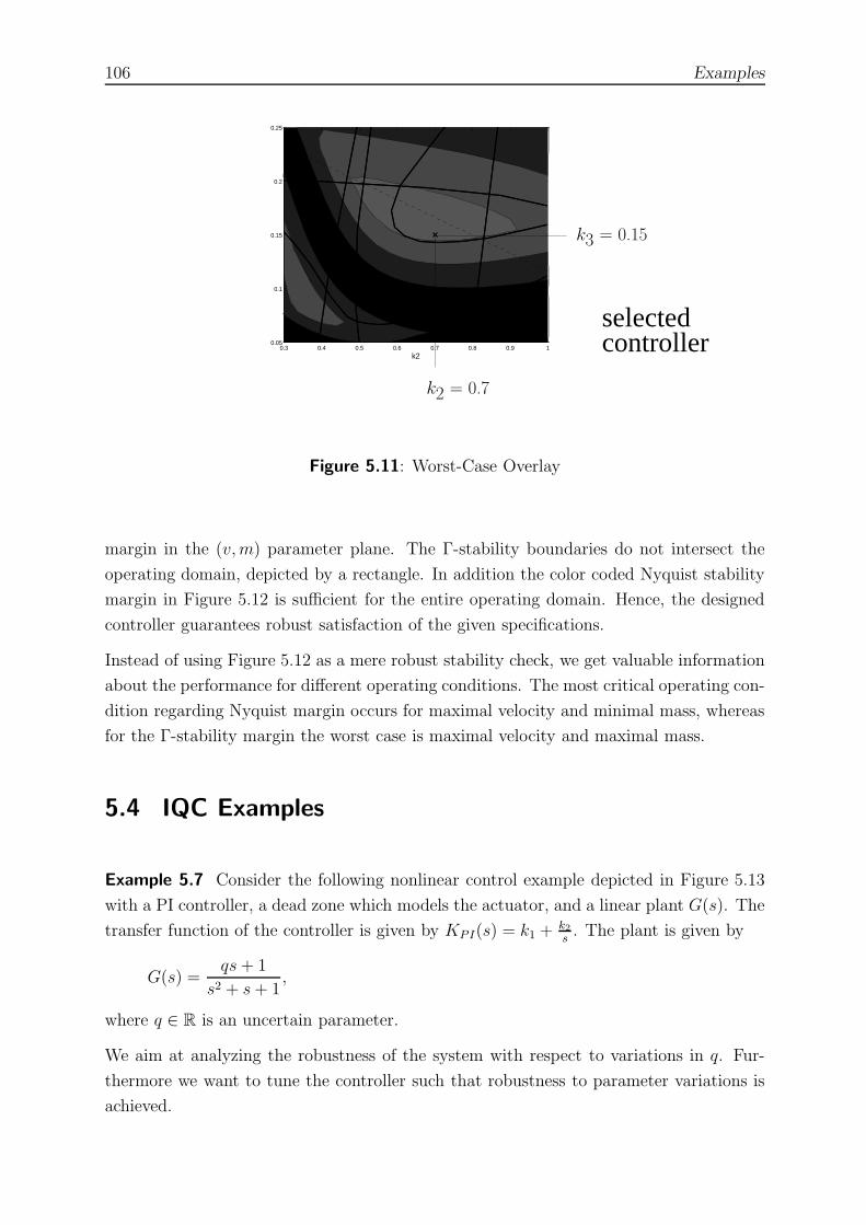
106 Examples
k20.3 0.4 0.5 0.6 0.7 0.8 0.9 1
0.05
0.1
0.15
0.2
0.25
controllerselected
k3 = 0.15
k2 = 0.7
Figure 5.11: Worst-Case Overlay
margin in the (v, m) parameter plane. The Γ-stability boundaries do not intersect the
operating domain, depicted by a rectangle. In addition the color coded Nyquist stability
margin in Figure 5.12 is sufficient for the entire operating domain. Hence, the designed
controller guarantees robust satisfaction of the given specifications.
Instead of using Figure 5.12 as a mere robust stability check, we get valuable information
about the performance for different operating conditions. The most critical operating con-
dition regarding Nyquist margin occurs for maximal velocity and minimal mass, whereas
for the Γ-stability margin the worst case is maximal velocity and maximal mass.
5.4 IQC Examples
Example 5.7 Consider the following nonlinear control example depicted in Figure 5.13
with a PI controller, a dead zone which models the actuator, and a linear plant G(s). The
transfer function of the controller is given by KPI(s) = k1 + k2
s. The plant is given by
G(s) =qs + 1
s2 + s + 1,
where q ∈ R is an uncertain parameter.
We aim at analyzing the robustness of the system with respect to variations in q. Fur-
thermore we want to tune the controller such that robustness to parameter variations is
achieved.

5.4 IQC Examples 107
v
m
Γ−stability and Frequency−Domain Analysis
0 5 10 15 20 25 30
5
10
15
20
25
30
35
40
45
50
Figure 5.12: Analysis in the operating domain
The given feedback interconnection is called critical since the worst case linearization is
at best neutrally stable. Note that the transfer function KPI(s)G(s) is unbounded which
prevents the application of standard stability criteria for nonlinear systems which require
bounded operators.
rPI G(s)
y
Figure 5.13: Dead zone PI controller example
We use the Zames-Falb IQC derived in [Jonsson and Megretski 1997], where it was shown
that an integrator and a sector bounded nonlinearity can be encapsulated in a bounded
operator that satisfies the following IQC
Π(jω) =
0 1 − H(jω)∗
1 − H(jω) − 2kRe(1 − H(jω)− kF (jω))
, (5.13)
where
F (s) =H(s) − H(0)
s,
where H(s) is a stable transfer function with L1 norm less than one, and the parameter k
equals the static gain of the open loop linear part k = k2G(0). This IQC corresponds to
the Zames-Falb IQC for slope restricted nonlinearities [Zames and Falb 1968].

108 Examples
Let the integral gain k2 = 2/5 and H(s) = 1/(s + 1). For our particular example the
parameter k equals the proportional gain k = k2. We map the stability condition into
the (k1, q) parameter plane. This allows to evaluate robustness with respect to q, while
we can select the controller gain k1 to maximize the robustness.
Since the multiplier Π(jω) in (5.13) is frequency-dependent, we use the method described
in Section 3.4.4 to reformulate the IQC stability problem with a constant multiplier.
The multiplier evaluates to
Π(jω) =
0jω
jω − 1
jω
jω + 1−5ω2 + 2
ω2 + 1
. (5.14)
This multiplier is not positive definite, so that most algorithms for spectral factorization
fail. A remedy is to use a constant offset matrix Π0 which makes the remainder positive
definite:
Π(jω) = Π0 + Πp(jω).
The transfer matrix Πp(jω) can now be factorized. So we alter (3.36) from Π(jω) =
Ψ(jω)∗ΠsΨ(jω), into Π(jω) = Ψ(jω)∗ΠsΨ(jω) + Π0, to get the spectral factorization
Π(jω) =
Ψ(jω)
I
∗
Πs 0
0 Π0
Ψ(jω)
I
,
which again has the form (3.36).
For this particular example the augmented system (A, B) in (3.43) is of forth order:
A =
−1 0 1 − q2 − 52k1 1 − 5
2k1q2
0 −1 0 0
0 0 0 1
0 0 −1 −1
, B =
0
1
0
1
,
and the submatrices Q, S and R of the multiplier M relevant for the mapping equations
are given as:
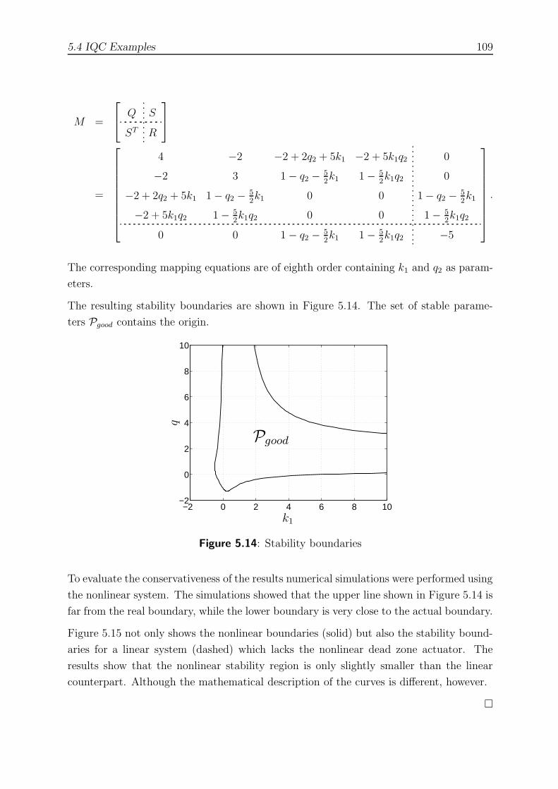
5.4 IQC Examples 109
M =
Q S
ST R
=
4 −2 −2 + 2q2 + 5k1 −2 + 5k1q2 0
−2 3 1 − q2 − 52k1 1 − 5
2k1q2 0
−2 + 2q2 + 5k1 1 − q2 − 52k1 0 0 1 − q2 − 5
2k1
−2 + 5k1q2 1 − 52k1q2 0 0 1 − 5
2k1q2
0 0 1 − q2 − 52k1 1 − 5
2k1q2 −5
.
The corresponding mapping equations are of eighth order containing k1 and q2 as param-
eters.
The resulting stability boundaries are shown in Figure 5.14. The set of stable parame-
ters Pgood contains the origin.
−2 0 2 4 6 8 10−2
0
2
4
6
8
10
PSfrag replacements
Pgood
k1
q
Figure 5.14: Stability boundaries
To evaluate the conservativeness of the results numerical simulations were performed using
the nonlinear system. The simulations showed that the upper line shown in Figure 5.14 is
far from the real boundary, while the lower boundary is very close to the actual boundary.
Figure 5.15 not only shows the nonlinear boundaries (solid) but also the stability bound-
aries for a linear system (dashed) which lacks the nonlinear dead zone actuator. The
results show that the nonlinear stability region is only slightly smaller than the linear
counterpart. Although the mathematical description of the curves is different, however.
�

110 Examples
−1 0 1 2 3−2
−1.5
−1
−0.5
0
0.5
1
1.5
2
PSfrag replacements
Pgood
k1
q
Figure 5.15: Comparison of linear and nonlinear system
5.5 Four Tank MIMO Example
A multivariable laboratory process is considered to show a practical application of the
robust control analysis and synthesis methods presented in this thesis. The process is
the level control of a system of four interconnected water tanks. The process has been
described in [Johansson 2000]. The system is shown in Figure 5.16. The system not only
shows considerable cross-couplings, but has an adjustable multivariable zero. Furthermore
it has static and dynamic nonlinearities.
The task is to control the water levels of the first and second tank by varying the flows
generated by the two pumps. The inputs are the control voltages for the pumps v1 and v2
and the outputs are level measurement voltages y1 and y2.
The nonlinear system model can be derived from mass balances and energy conservation
in the form of Bernoulli’s law for flows of incompressible, non-viscous fluids
h1 = − a1
A1
√
2gh1 +a3
A1
√
2gh3 +γ1k1
A1
v1
h2 = − a2
A2
√
2gh2 +a4
A2
√
2gh4 +γ2k2
A2
v2
h3 = − a3
A3
√
2gh3 +(1 − γ2)k2
A3
v2
h4 = − a4
A4
√
2gh4 +(1 − γ1)k1
A4
v1,
(5.15)
where Ai is the cross-section of tank i, ai the cross-section of outlet i, and hi the water
level of the i-th tank. The output signals for the measured levels are proportional to the
water level y1 = kch1 and y2 = kch2.

5.5 Four Tank MIMO Example 111
Tank 2
Tank 4Tank 3
γ2v2γ1v1
Tank 1
Pump 1 Pump 2
v1 v2
(1− γ1)v1 (1− γ2)v2
Figure 5.16: Schematic diagram of the four-tank process
The transfer matrix linearized for a given static operating point is
G(s) =
γ1c11
(T1s + 1)
(1 − γ2)c12
(T1s + 1)(T3s + 1)
(1 − γ1)c21
(T2s + 1)(T4s + 1)
γ2c22
(T2s + 1)
. (5.16)
Let the ratio of water diverted to tank one rather than tank three be γ1 = 0.33 and
the corresponding ratio of pump two is set to γ2 = 0.167. All other nominal parameter
values are given in Table 5.1. The transfer matrix (5.16) then has two multivariable
zeros at s = −0.197 and s = 0.118. The multivariable RHP zero limits the achievable
performance for this system.
Table 5.1: Parameter values for four tank example
A1, A2, A3, A4 [cm2] [30.0, 30.0, 20.0, 20.0]
a1, a2, a3, a4 [cm2] [0.1, 0.067, 0.067, 0.1]
k1, k2 [cm3/Vs] 3.0
kc [V/cm] 1.0

112 Examples
We consider decentralized PI control with input-output pairing y1 − u2 and y2 − u1 sug-
gested by relative gain array analysis. Here, we link both Kp and Ki parameters of the
individual loops, i.e. Kp = Kp1 = Kp2 and Ki = Ki1 = Ki2 and map a real part limitation
of Re s < 0.004 and a nominal performance ||WpS||∞ specification, where S is the sensi-
tivity and Wp = (250s+10)/(1000s+1) a performance weighting function. The resulting
plot is shown in Figure 5.17 where good performance is represented by light colors and
the eigenvalue specification is depicted by dashed lines.
Taking an optimal value from Figure 5.17 the resulting multivariable controller can be
fine-tuned, for example by considering the individual loops or by evaluating robustness
with respect to changes in the nominal parameter values.
0 0.2 0.4 0.6 0.8 1 1.2 1.4 1.6 1.8 2
0.002
0.004
0.006
0.008
0.01
0.012
0.014
0.016
0.018
Four tank PI controller design
Kp
Ki
Figure 5.17: PI controller design for four tank example

113
6 Summary and Outlook
We conclude with a brief summary of the work presented, and remarks on future directions
for related research.
6.1 Summary
Robust control of systems with real parameter uncertainties is a topic of practical impor-
tance in control engineering. In this thesis we considered the mapping of new specifica-
tions. Although well-known and often used, some of these specifications have not been
used in the parameter space context. Furthermore, the considered specifications can be
mapped for multivariable systems. Special criteria for nonlinear systems are presented.
To this end, not only standard specifications like the Popov criterion are considered, but
the mapping of versatile integral quadratic constraints is introduced.
Starting point of the thesis is the observation that many practical specifications, for exam-
ple H∞ norm and passivity, can be formulated using the same mathematical framework.
Namely algebraic Riccati equations (AREs). An important link forms the KYP lemma,
which translates different mathematical formulations of specifications into each other.
A corresponding set of specifications can be formulated using Lyapunov equations, a spe-
cial case of an ARE. Important representatives are the H2 norm and LQR specifications.
These allow to express performance specifications in parameter space. These specifica-
tions directly lead to a single implicit mapping equation, which is in general at least
quadratic in the uncertain parameters.
Mathematical results on the analytic dependence of solutions for parametric AREs led to
the derivation of mapping equations. Hereby control specifications formulated as AREs
can be converted into a specific eigenvalue problem using properties of associated Hamil-
tonian matrices.
The introduction of mapping equations for IQCs broadens the applicable system class even
further by enabling to consider specifications for input-output theory, absolute stability
theory, and the robust control field. The exploitation of additional degrees of freedom
provided by variable uncertainty characterization is shown.

114 Summary and Outlook
Mapping equations for ARE and Lyapunov equation based specifications are similar in
structure to root locus specifications. Nevertheless, due to the quadratic nature of the
specifications, which shows in the AREs, the mapping equations are in general more
complex and nontrivial to solve.
Practical aspects of the thesis therefore include the presentation of a hybrid symbolic-
numerical algorithm. This algorithm exploits the properties of the algebraic mapping
equations to determine characteristic points on the resulting curves in a parameter plane.
The topology of the curve then allows to either numerically connect the individual curve
points by curve following or to approximate the curve using a Bezier approximation. The
uniform mathematical description of the mapping equations allows to employ a single
mapping algorithm for all specifications.
The mapping equations are based on a parametric state-space realization. A symbolic
algorithm is hereto presented, which calculates a state-space realization for a given transfer
function.
This thesis shows that classical eigenvalue criteria and modern norm and nonlinear spec-
ifications can be combined in the parameter space approach to yield an efficient control
engineering tool that takes all practical aspects like stability, performance and robustness
into account.
6.2 Outlook
We note related future research topics.
In this thesis, a comprehensive methodology to map control specifications into parameter
spaces is presented. The successful and wide-spread use of these methods necessitates
an efficient and robust software implementation of the given algorithms. Furthermore, a
user-friendly front-end facilitates the practical application of the thesis results. It can be
used to specify the considered system and corresponding specifications and to evaluate the
graphical results. One possible way is a computer toolbox with graphical user interaction.
While the new possibilities have been demonstrated on some practical examples, one line
of research is to apply the methods to a large-scale real-world problem and to investigate
the limits and computational burdens.
There are numerous ways to characterize uncertainty. While the approach pursuit in this
thesis is to deal explicitly with real uncertain parameters, one research topic is to evaluate
different uncertainty characterizations.

115
A Mathematics
This appendix reviews some mathematical topics used in the thesis, that are not neces-
sarily treated in graduate level engineering courses. Particularly all theorems needed to
prove the fundamental theorems in Chapter 3 are stated here.
We shall always work with finite dimensional Euclidean spaces, where
Rn = {(x1, . . . , xn) : x1, . . . , xn ∈ R},Cn = {(x1, . . . , xn) : x1, . . . , xn ∈ C}.
A point in Rn is denoted by x = (x1, . . . , xn) and the coordinate or natural basis vectors
are written as ei :
e1 =
1
0...
0
, e2 =
0
1...
0
, . . . , en =
0
0...
1
.
All arguments of functions are either given in parenthesis or omitted for brevity.
A.1 Algebra
This section reviews basic facts from tensor algebra. The use of tensors facilitates the
notation of matrix derivatives used for some algorithms presented in Chapter 4. Fur-
thermore tensors are supported by symbolic and numerical software packages such as
Matlab and Maple and therefore allow an easy implementation of the presented algo-
rithms. See [Graham 1981] for a good reference on tensor algebra.
Given two matrices A ∈ CnA,mA , B ∈ CnB ,mB , the Kronecker product matrix of A and B,
denoted by A ⊗ B ∈ CnA∗nB ,mA∗mB , is defined by the partitioned matrix
A ⊗ B :=
a11B a12B · · · a1mAB
a21B a22B · · · a2mAB
...... · · ·
...
anA1B anA2B · · · anAmAB
.
116 Mathematics
The Kronecker power of a matrix is defined similar to the standard matrix power as
X⊗,2 = X ⊗ X, X⊗,3 = X ⊗ X⊗,2, X⊗,i = X ⊗ X⊗,i−1, (A.1)
where the superscript ⊗, i denotes the i-th Kronecker power.
The Kronecker sum of two matrices A ∈ CnA, nA B ∈ CnB , nB is defined as
A ⊕ B := A ⊗ InB+ InA
⊗ B,
where In is the identity matrix of order n.
Furthermore, let vec(X) denote the vector that is formed by stacking the columns of X
into a single column vector:
vec(X) :=[
x11 x21 . . . xm1 x1n x2n . . . xmn
]T .
Using this stacking operator the following properties hold for complex1 matrices with
matching dimensions:
vec(AXB) = (BT ⊗ A) vec(X),
and
vec(AX + XB) = (BT ⊕ A) vec(X).
A.2 Algebraic Riccati Equations
This section will review important facts about algebraic Riccati equations (AREs). In
order to make this section rather self-contained we will state theorems presenting basic
properties of AREs.
The general algebraic matrix Riccati equation is given by
XRX − XP − P ∗X − Q = 0 , (A.2)
where R, P and Q are given n×n complex matrices with R and Q Hermitian, i.e., R = R∗
and Q = Q∗.
Together with (A.2) we will consider the matrix function
R(X) = XRX − XP − P ∗X − Q. (A.3)
1Note that T denotes the transpose, while ∗ is used for the complex conjugate transpose
A.2 Algebraic Riccati Equations 117
Associated with (A.2) is a 2n × 2n Hamiltonian matrix:
H :=
−P R
Q P ∗
. (A.4)
The following theorem [Zhou et al. 1996] gives a constructive description of all solutions
to (A.2).
Theorem A.1 ARE solutions
Let V ⊂ C2n be an n-dimensional invariant subspace of H, and let X1, X2 ∈ Cn×n
be two complex matrices such that
V = Im
X1
X2
.
If X1 is invertible, then X = X2X−11 is a solution to the Riccati equation (A.2)
and Λ(P − RX) = Λ(H|V), where H|V denotes the restriction of H to V.
�
Proof:
We only show the first part of the theorem that proofs the construction of solutions.
The following equation holds because V is an M invariant subspace:
−P R
Q P ∗
X1
X2
=
X1
X2
Λ.
Premultiply the above equation by [X −I ] and then postmultiply with X−11 to get
[
X −I]
−P R
Q P ∗
I
X
= 0 ,
XRX − XP − P ∗X − Q = 0 .
This shows that X = X2X−11 is actually a solution of (A.2).
�
118 Mathematics
Theorem A.1 shows that we can determine all solutions of (A.2) by constructing bases for
those invariant subspaces of H. For example, the invariant subspaces can be found by com-
puting the eigenvectors vi and corresponding generalized eigenvectors vi+1, . . . , vi+ki−1
related to eigenvalues λi of H with multiplicity ki. Taking all combinations of these vec-
tors, which have at least one actual eigenvector vi and are therefore H invariant, we can
calculate the solutions X = X2X−11 from
X1
X2
=[
vi vj
]
, i 6= j.
Before we turn to the important stabilizing solutions of an ARE, we consider maximal
solutions. The following theorem will be used in the proof of Theorem A.3 also.
Theorem A.2 Maximal solutions
Suppose that R = R∗ ≥ 0, Q = Q∗, (P, R) is stabilizable, and there is a Hermitian
solution of the inequality R(X) ≤ 0. Then R(X) = 0 has a maximal Hermitian
solution X+ for which X+ ≥ X for every Hermitian solution X of R(X) ≤ 0 holds.
Furthermore the maximal solution X+ guarantees that all eigenvalues of P − RX+
lie in the closed left half-plane.
�
See [Kleinman 1968], [Lancaster and Rodman 1995, p. 232] or [Zhou et al. 1996] for a
proof. The proof is constructive, i.e., it not only proofs the preceding statements, but
it also gives an iterative procedure to determine the maximal solution X+. A Newton
procedure can be derived to solve the equation R(X) = 0.
Decompose R into R = BB∗. Since the pair (P, R) is stabilizable, it can be seen from
the controllability matrix that the pair (P, B) is also stabilizable and there is a stabilizing
feedback matrix F0 for which P0 = P − BF0 is stable.
Then we determine X0 as the unique, Hermitian solution of the Lyapunov equation
X0P0 + P ∗0 X0 + F ∗
0 F0 + Q = 0.
In order to apply the Newton procedure to the matrix function R(X), we need the first
Frechet derivative [Ortega and Rheinboldt 1970]:
dRX(H) = −(H(P − RX) + (P − RX)∗H).
The Newton procedure is than given as
dRX(Xk+1 − Xk) = −R(Xk), k = 0, 1, 2, . . . (A.5)

A.2 Algebraic Riccati Equations 119
This can be written as the following Lyapunov equation,
Xk+1(P − RXk) + (P − RXk)∗Xk+1 = −XkRXk − Q, k = 0, 1, 2, . . . (A.6)
We can now finally turn to the important Theorem 3.1 which forms the basis for the
mapping equations, because it converts conditions for an ARE into an eigenvalue problem.
The theorem is restated here, see [Lancaster and Rodman 1995, p. 196]. The actual
mapping equations can be derived using the analytic extension given by Lancaster and
Rodman in 1995.
Theorem A.3 Stabilizing solutions
Suppose that R ≥ 0, Q = Q∗, (P, R) is stabilizable, and there is a Hermitian solution
of (A.2). Then for the maximal Hermitian solution X+ of (A.2), P −RX+ is stable,
if and only if the Hamiltonian matrix H defined in (A.4) has no eigenvalues on the
imaginary axis.
�
Proof:
Since the pair (P, R) is only required to be stabilizable, we start with a decomposi-
tion into a controllable and stable part, such that the matrices P , R, Q, and X can
be written as
P =
P11 P12
0 P22
, R =
R11 0
0 0
, Q =
Q11 Q12
Q∗12 Q22
, X =
X11 X12
X∗12 X22
, (A.7)
where the pair (P11, R11) is controllable and P22 is stable. This decomposition leads
to a Riccati equation in standard form for the controllable pair (P11, R11)
X11R11X11 − X11P11 − P ∗11X11 − Q11 = 0 , (A.8)
a Sylvester equation in X12, and a Lyapunov equation in X22. Furthermore the
term P − RX can be written as
P − RX =
P11 − R11X11 P12 − R11X12
0 P22
, (A.9)
and the ARE (A.8) has the associated Hamiltonian H11.
We are now ready to proof that stability of P − RX+ follows from H having not a
single pure imaginary eigenvalue. To this end, suppose that H has no eigenvalues
on the imaginary axis. The decomposition above leads to
Λ(H) = Λ(H11) ∪ Λ(−P22) ∪ Λ(P ∗22), (A.10)
120 Mathematics
and any solution X11 of (A.8) has the property Λ(P11 − R11X11) ⊆ Λ(H11). Using
Theorem A.2 it follows that (A.8) has a maximal solution X+11, and Λ(P11−R11X
+11)
is stable. From the triangular decomposition and in particular (A.9) then follows
that P − RX+ holds for the corresponding solution X+ of (A.2).
To proof the converse, assume that X+ is a maximal solution of (A.2) and P −RX+
is stable. Let X+ be decomposed similar to X in (A.7). From (A.9) then follows
that P11 − R11X+11 is stable and that X+
11 is a maximal solution of (A.8). There-
fore H11 has no pure imaginary eigenvalues and the proof is concluded, since (A.10)
implies that the same holds for H.
�
References 121
References
Ackermann, J., Der Entwurf linearer Regelungssysteme im Zustandsraum, Regelungstech-
nik, 1972, vol. 20, pp. 297–300.
Ackermann, J., Parameter space design of robust control systems, IEEE Trans. on Auto-
matic Control, 1980, vol. 25, pp. 1058–1072.
Ackermann, J., A. Bartlett, D. Kaesbauer, W. Sienel, and R. Steinhauser, Robust Control,
Springer-Verlag, 1993.
Ackermann, J., P. Blue, T. Bunte, L. Guvenc, D. Kaesbauer, M. Kordt, M. Muhler,
and D. Odenthal, Robust Control: The Parameter Space Approach, Springer-Verlag,
London, 2002.
Ackermann, J. and T. Bunte, Robust Prevention of Limit Cycles for Robustly Decoupled
Car Steering Dynamics, Kybernetika, 1999, vol. 35, no. 1, pp. 105–116.
Ackermann, J., D. Kaesbauer, and R. Munch, Robust Γ-stability analysis in a plant pa-
rameter space, Automatica, 1991, vol. 27, pp. 75–85.
Ackermann, J. and W. Sienel, Robust control for automatic steering, in Proc. American
Control Conf., San Diego, 1990, pp. 795–800.
Ackermann, J. and S. Turk, A common controller for a family of plant models, in Proc.
IEEE Conf. on Decision and Control, Orlando, 1982, pp. 240–244.
Allgower, E. L. and K. Georg, Numerical Continuation Methods, Springer-Verlag, 1990.
Allgower, E. L. and K. Georg, Continuation and Path Following, Acta Numerica, 1992,
vol. 2, pp. 1–64.
Anderson, B. D. O., A system theory criterion for positive real matrices, SIAM Journal
on Control, 1967, vol. 5, pp. 171–182.
Anderson, B. D. O. and S. Vongpanitlerd, Network Analysis and Synthesis: A Modern
Systems Theory Approach, Prentice-Hall, 1973.

122 References
Arnon, D. S. and S. McCallum, A polynomial time algorithm for the topological type of a
real algebraic curve, Journal of Symbolic Computation, 1988, vol. 5, pp. 213–236.
Barmish, B. R., J. Ackermann, and H. Z. Hu, The tree structured decomposition: a
new approach to robust stability analysis, in Proc. Conf. on Information Sciences and
Systems, Princeton, 1990a, pp. 133–139.
Barmish, B. R., P. P. Khargonekar, Z. C. Shi, and R. Tempo, Robustness margin need
not be a continuous function of the problem data, Systems and Control Letters, 1990b,
vol. 15, pp. 91–98.
Bart, H., I. Gohberg, and M. A. Kaashoek, Constructive Methods of Wiener-Hopf Fac-
torization, Birkhauser, 1986.
Beckermann, B. and G. Labahn, Numeric and Symbolic Computation of problems defined
by Structured Linear Systems, Reliable Computing, 2000, vol. 6, pp. 365–390.
Besson, V. and A. T. Shenton, Interactive Control System Design by a mixed H∞ Pa-
rameter Space Method, IEEE Trans. on Automatic Control, 1997, vol. 42, no. 7, pp.
946–955.
Besson, V. and A. T. Shenton, An Interactive Parameter Space Method For Robust Per-
formance in Mixed Sensitivity Problems, IEEE Trans. on Automatic Control, 1999,
vol. 44, no. 6, pp. 1272–1276.
Boyd, S., Robust Control Tools: Graphical User-Interfaces and LMI Algorithms, Systems,
Control and Information, 1994, vol. 38, no. 3, pp. 111–117, special issue on Numerical
Approaches in Control Theory.
Boyd, S., V. Balakrishnan, and P. Kabamba, A bisection method for computing the H∞
norm of a transfer matrix and related problems, Mathematics of Control, Signals and
Systems, 1989, vol. 2, no. 3, pp. 207–219.
Boyd, S. and C. Barratt, Linear Controller Design: Limits of Performance, Prentice-Hall,
1991.
Boyd, S., L. E. Ghaoui, E. Feron, and V. Balakrishnan, Linear Matrix Inequalities in
System and Control Theory, SIAM studies in applied mathematics, 1994.
Boyd, S. and Q. Yang, Structured and Simultaneous Lyapunov Functions for System
Stability Problems, Int. Journal of Control, 1989, vol. 49, no. 6, pp. 2215–2240.
Bunte, T., Mapping of Nyquist/Popov Theta-stability margins into parameter space, in
Proc. 3rd IFAC Symp. on Robust Control Design, Prague, Czech Republic, 2000.

References 123
Chen, C. T., Linear System Theory and Design, Hold, Rinehart and Winston, New York,
1984.
Coolidge, J. L., A Treatise on Algebraic Plane Curves, Dover Publications, 2004.
Davidenko, D., On a new method of numerical solution of systems of nonlinear equations
(in Russian), Dokl. Akad. Nauk USSR, 1953, vol. 88, pp. 601–602.
Doyle, J. C., Guaranteed margins for LQG regulators, IEEE Trans. on Automatic Control,
1978, vol. 23, no. 4, pp. 756–757.
Doyle, J. C., Analysis of feedback systems with structured uncertainties, IEE Proc., 1982.
Doyle, J. C., Redondo Beach lecture notes, Internal Report, Caltech, Pasadena, 1986.
Doyle, J. C., K. Glover, P. Khargonekar, and B. Francis, State-space solution to standard
H2 and H∞ control problems, IEEE Trans. on Automatic Control, 1989, vol. 34, no. 8,
pp. 831–847.
Doyle, J. C. and G. Stein, Multivariable feedback design: Concepts for a classical/modern
synthesis, IEEE Trans. on Automatic Control, 1981, vol. 26, no. 1, pp. 4–16.
Earnshaw, R. A. and N. Wiseman, An Introductory Guide to Scientific Visualization,
Springer, 1992.
Evans, W. R., Graphical analysis of control systems, Trans. AIEE, 1948, vol. 67, no. 2,
pp. 547–551.
Farin, G., Curves and Surfaces for Computer Aided Geometric Design, Morgan Kauf-
mann, 2001.
Forsman, K. and J. Eriksson, Solving the ARE symbolically, Technical Report LiTH-ISY-
R-1456, Dept. of Electrical Engineering, Linkoping University, 1993.
Francis, B., A course in H∞ control theory, Springer, New-York, 1987.
Gajic, Z. and M. Qureshi, Lyapunov Matrix Equation in System Stability and Control,
Mathematics in Science and Engineering Series, Academic Press, 1995.
Gilbert, E. G., Controllability and observability in multi-variable control systems, Int.
Journal of Control, 1963, vol. 1, no. 2, pp. 128–151.
Glover, K., All optimal Hankel-norm approximation of linear multivarible systems and
their L∞- error bounds, Int. Journal of Control, 1984, vol. 39, pp. 1115–1193.
124 References
Gonzalez-Vega, L. and I. Necula, Efficient topology determination of implicitly defined
algebraic plane curves, Computer Aided Geometric Design, 2002, vol. 19, no. 9, pp.
719–743.
Graham, A., Kronecker Products and Matrix Calculus with Applications, J. Wiley & Sons,
1981.
Green, M., K. Glover, D. Limebeer, and J. C. Doyle, A J-spectral approach to H∞ control,
SIAM Journal on Control and Optimization, 1990, vol. 28, pp. 1350–1371.
Haddad, W. M. and D. S. Bernstein, Robust stabilization with positive real uncertainty:
Beyond the small gain theorem, Systems and Control Letters, 1991, vol. 17, pp. 191–208.
Hara, S., T. Kimura, and R. Kondo, H∞ control system design by a parameter space
approach, in Proc. 10th Int. Symp. on Mathematical Theory of Networks and Systems,
Kobe, Japan, 1991, pp. 287–292.
Hermite, C., Sur le nombre des racines d’une equation algebrique comprise entre des
limites donnees, J. Reine Angewandte Mathematik, 1856, vol. 52, pp. 39–51, English
translation Int. Journal of Control 1977.
Hinrichsen, D. and A. J. Pritchard, Stability radius for structured perturbations and the
algebraic Riccati equation, Systems and Control Letters, 1986, vol. 8, pp. 105–113.
Hurwitz, A., Ueber die Bedingungen, unter welchen eine Gleichung nur Wurzeln mit
negativen reellen Theilen besitzt, Mathematische Annalen, 1895, vol. 46, pp. 273–284.
Johansson, K. H., The Quadruple-Tank Process: A Multivariable Laboratory Process with
an Adjustable Zero, IEEE Trans. on Control Systems Technology, 2000, vol. 8, no. 3,
pp. 456–465.
Jonsson, U., A Popov Criterion for Systems with Slowly Time-Varying Parameters, IEEE
Trans. on Automatic Control, 1999, vol. 44, no. 4, pp. 844–846.
Jonsson, U., Lectures on Input-Output Stability and Integral Quadratic Constraints, Lec-
ture Notes, Royal Institute of Technology, Stockholm, Sweden, 2001.
Jonsson, U. and A. Megretski, The Zames-Falb IQC for Critically Stable Systems, Tech-
nical report, MIT, 1997.
Joos, H.-D., A. Varga, and R. Finsterwalder, Multi-Objective Design Assessment, in IEEE
Symp. on Computer-Aided Control System Design, Kohala, Hawaii, USA, 1999.
Kabamba, P. T. and S. P. Boyd, On parametric H∞ optimization, in Proc. IEEE Conf.
on Decision and Control, Austin, Texas, 1988, vol. 4, pp. 1354–1355.

References 125
Kailath, T., Linear Systems, Prentice-Hall, 1980.
Kalman, R. E., Mathematical description of linear dynamical systems, SIAM Journal on
Control, 1963.
Kalman, R. E. and R. S. Bucy, New results in linear filtering and prediction theory, ASME
Trans. Series D: J. Basic Engineering, 1960, vol. 83, pp. 95–108.
Khalil, H. K., Nonlinear Systems, Macmillan, 1992.
Kleinman, D. L., On an iterative technique for Riccati equation computation, IEEE Trans.
on Automatic Control, 1968, vol. 13, pp. 114–115.
Kugi, A. and K. Schlacher, Analysis and Synthesis of Non-linear Dissipative Systems:
An Overview (Part 2) (in German), Automatisierungstechnik, 2002, vol. 50, no. 3, pp.
103–111.
Kwakernaak, M. A. and R. Sivan, Linear Optimal Control Systems, Wiley-Interscience,
1972.
Lancaster, P. and L. Rodman, Existence and uniqueness theorem for the algebraic Riccati
equation, Int. Journal of Control, 1980, vol. 32, no. 2, pp. 285–309.
Lancaster, P. and L. Rodman, Algebraic Riccati equations, Oxford Science Publications,
1995.
Laub, A. J., A Schur method for solving the algebraic Riccati equations, IEEE Trans. on
Automatic Control, 1979, vol. 24, pp. 913–925.
Lind, R. and M. J. Brenner, Robust Flutter Margin Analysis that Incorporates Flight Data,
Technical report, NASA, 1998.
Lunze, J., Robust Multivariable Feedback Control, Prentice-Hall, London, 1988.
Maciejowski, J. M., Multivariable Feedback Design, Electronic Systems Engineering Series,
Addison-Wesley, 1989.
Magni, J. F., Linear Fractional Representations with a Toolbox for Use with MATLAB,
Toolbox Manual, ONERA, Technical Report TR 240/01 DCSD, 2001.
Maxwell, J. C., On Governors, Proc. Royal Soc. London, 1866, vol. 16, pp. 270–283.
McFarlane, D. and K. Glover, Robust Controller Design Using Normalized Coprime Factor
Plant Descriptions, vol. 138 of Lecture Notes in Control and Information Sciences,
Springer-Verlag, 1990.

126 References
Megretski, A. and A. Rantzer, System analysis via integral quadratic constraints, IEEE
Trans. on Automatic Control, 1997, vol. 42, no. 6, pp. 819–830.
Mitrovic, D., Graphical analysis and synthesis of feedback control systems, Trans. AIEE,
1958, vol. 77, no. 2, pp. 476–503.
Morgan, A., Solving polynomial systems using continuation for engineering and scientific
problems, Prentice-Hall, 1987.
Muhler, M., Mapping MIMO Control Specifications into Parameter Space, in Proc. IEEE
Conf. on Decision and Control, Las Vegas, NV, 2002, pp. 4527–4532.
Muhler, M. and J. Ackermann, Representing multiple objectives in parameter space us-
ing color coding, in Proc. 3rd IFAC Symp. on Robust Control Design, Prague, Czech
Republic, 2000.
Muhler, M. and J. Ackermann, Mapping Integral Quadratic Constraints into Parameter
Space, in Proc. American Control Conf., Boston, MA, 2004, pp. 3279–3284.
Muhler, M. and D. Odenthal, Paradise: Ein Werkzeug fur Entwurf und Analyse robuster
Regelungssysteme im Parameterraum, in 3. VDI/VDE-GMA Aussprachetag, Rechn-
ergestutzter Entwurf von Regelungssystemen, Dresden, 2001.
Muhler, M., D. Odenthal, and W. Sienel, Paradise User’s Manual, Deutsches Zentrum
fur Luft und Raumfahrt e. V., Oberpfaffenhofen, 2001.
Mustafa, D. and K. Glover, Minimum Entropy H∞ Control, Lecture Notes in Control and
Information Sciences, Springer-Verlag, 1990.
Odenthal, D. and P. Blue, Mapping of frequency response magnitude specifications into
parameter space, in Proc. 3rd IFAC Symp. on Robust Control Design, Prague, Czech
Republic, 2000.
Ortega, J. M. and W. C. Rheinboldt, Iterative solution of nonlinear equations in several
variables, Academic Press, New York, 1970.
Otter, M., Objectoriented Modeling of Physical Systems (in German), Automatisierung-
stechnik, 1999, vol. 47/48, series ”Theorie fur den Anwender”, 17 parts from 1/1999 to
12/2000.
Owen, J. G. and G. Zames, Robust H∞ disturbance minimization by duality, Systems and
Control Letters, 1992, vol. 19, no. 4, pp. 255–263.
Petersen, I. R., Disturbance attenuation and H∞-optimization: A design method based on
the algebraic Riccati equations, IEEE Trans. on Automatic Control, 1987, vol. 32, pp.
427–429.
References 127
Poincare, H., Les Methodes Nouvelles de la Mecanique Celeste, Gauthier-Villars, Paris,
1892.
Ran, A. C. M. and L. Rodman, On parameter dependence of solutions of algebraic Riccati
equations, Mathematics of Control, Signals and Systems, 1988, vol. 1, pp. 269–284.
Rantzer, A., On the Kalman-Yakubovich-Popov lemma, Systems and Control Letters,
1996, vol. 28, pp. 7–10.
Rosenbrock, H. H., State-space and multivariable theory, Nelson, London, 1970.
Rotea, M. A., The generalized H2 control problem, Automatica, 1993, vol. 29, no. 2, pp.
373–385.
Routh, E. J., A Treatise on the Stability of a Given State of Motion, Macmillan, London,
1877.
Safonov, M. G., Stability margins of diagonally perturbed multivariable feedback systems,
IEE Proc., 1982.
Safonov, M. G. and V. V. Kulkarni, Zames-Falb Multipliers for MIMO Nonlinearities,
Int. Journal of Nonlinear and Robust Control, 2000.
Sakkalis, T., The topological configuration of a real algebraic curve, Bulletin of the Aus-
tralian Mathematical Society, 1991, vol. 43, no. 1, pp. 37–50.
Sandberg, I. W., On the L2-boundedness of solutions of nonlinear functional equations,
Bell Syst. Tech. J., 1964.
Scherer, C., P. Gahinet, and M. Chilali, Multiobjective output-feedback control via LMI
optimization, IEEE Trans. on Automatic Control, 1997, vol. 42, no. 7, pp. 896–911.
Schmid, C., Zur direkten Berechnung von Stabilitatsrandern, Wurzelortskurven und H∞-
Normen, Habilitationsschrift, Fortschritt-Berichte, Reihe 8, Nr. 367, VDI-Verlag, 1993,
(In German).
Sepulchre, R., M. Jankovic, and P. Kokotovic, Constructive Nonlinear Control, Springer-
Verlag, London, 1997.
Sienel, W., T. Bunte, and J. Ackermann, Paradise - A Matlab-based robust control
toolbox, in Proc. IEEE Symp. on Computer-Aided Control System Design, Dearborn,
MI, 1996, pp. 380–385.
Skogestad, S. and I. Postlethwaite, Multivariable Feedback Control, John Wiley & Sons,
1996.

128
Tiller, M., Introduction to Physical Modeling with Modelica, Kluwer Academic Publishers,
Boston, 2001.
van Hoeij, M., Rational Parametrizations of Algebraic Curves using a Canonical Divisor,
Journal of Symbolic Computation, 1997, vol. 23, pp. 209–227.
Varga, A. and G. Looye, Symbolic and numerical software tools for LFT-based low order
uncertainty modeling, in IEEE Int. Symp. on Computer-Aided Control System Design,
Hawaii, 1999, pp. 1–6.
Vidyasagar, M., Nonlinear System Analysis, Prentice-Hall, 1978.
Vishnegradsky, I. A., Sur la theorie generale des regulateurs, Compt. Rend. Acad. Sci.,
1876, vol. 83, pp. 318–321.
Walker, R. J., Algebraic Curves, Springer, 1978.
Willems, J. C., Least squares stationary optimal control and the algebraic Riccati equation,
IEEE Trans. on Automatic Control, 1971, vol. 16, no. 6, pp. 621–634.
Wilson, D. A., Convolution and Hankel operator norms for linear systems, IEEE Trans.
on Automatic Control, 1989, vol. 34, no. 1, pp. 94–97.
Zames, G., Feedback and optimal sensitivity: model reference transformations, multiplica-
tive seminorms, and approximate inverse, IEEE Trans. on Automatic Control, 1981,
vol. 26, pp. 301–320.
Zames, G. and P. L. Falb, Stability conditions for systems with monotone and slope-
restricted nonlinearities, SIAM Journal on Control, 1968, vol. 6, no. 1, pp. 89–108.
Zhou, K., J. C. Doyle, and K. Glover, Robust and optimal control, Prentice-Hall, 1996.

129
Lebenslauf
Michael Ludwig Muhler
geboren am 3. Februar 1973 in Creglingen
verheiratet, ein Kind
September 1983 - Mai 1992 Gymnasium Weikersheim
Oktober 1993 - Juli 1997 Studium der Technischen Kybernetik
an der Universitat Stuttgart
August 1997 - September 1998 Graduate Studies
in Chemical and Electrical Engineering
University of Wisconsin, Madison
Oktober 1998 - Januar 1999 Studium der Technischen Kybernetik
an der Universitat Stuttgart
Januar 1999 - August 2002 Wissenschaftlicher Mitarbeiter beim
Deutschen Zentrum fur Luft- und Raumfahrt
Oberpfaffenhofen
Institut fur Robotik und Mechatronik
seit September 2002 Mitarbeiter der Robert Bosch GmbH
Stuttgart
Korntal-Munchingen, im Marz 2007


![A Yield Mapping Procedure Based on Robust Fitting ...a paraboloid cone are estimated by robust weighted M-estimators (cf. Hampel et al. [10], Section 6.3) so that the influence of](https://static.fdocuments.us/doc/165x107/5e647043cb479e37f92b5957/a-yield-mapping-procedure-based-on-robust-fitting-a-paraboloid-cone-are-estimated.jpg)