
Lecture 17 Network Layer (Virtual Circuits, Datagrams, Routers)
Forwarding Strategies for6LoWPAN-Fragmented IPv6 Datagrams
Vom Promotionsausschuss derTechnischen Universitat Hamburg-Harburg
zur Erlangung des akademischen Grades
Doktor-Ingenieur (Dr.-Ing.)
genehmigte Dissertation
vonAndreas Weigel
ausPotsdam, Deutschland
2017

Date of Oral Examination September 05th, 2017
Chair of Examination Board Prof. Dr. Heiko Falk
Institute of Embedded SystemsHamburg University of Technology
First Examiner Prof. Dr. Volker Turau
Institute of TelematicsHamburg University of Technology
Second Examiner Prof. Dr. Andreas Timm-Giel
Institute of Communication NetworksHamburg University of Technology

Acknowledgment
Several people supported me in the long, difficult and sometimes frustrating processof finishing this dissertation. I want to seize the opportunity to express my deeply feltgratitude towards them.
First, I would like to thank my supervisor Prof. Turau for his guidance, encourage-ment and intellectual input, but also for being the kind of superior he is.
I would like to thank my colleagues, who made everydays work at the institute apleasant experience. Special thanks go to my “roommates” Bernd-Christian Renner,Martin Ringwelski and Florian Kauer for bearing with me and my curses and com-plains and for providing so much valuable input. Further, I’d like to thank StefanUnterschutz and Martin Ringwelski for their implementation work on CometOS andits 6LoWPAN module and the numerous fruitful discussions.
I want to thank my parents for their genes and the continuous support I experiencedthroughout my life. And finally: Thanks Susanne, for your encouragement and helpand for taking on life together with me.
Andreas WeigelLuneburg, November 2017


Abstract
Recent efforts towards a fully standardized protocol stack (RPL, CoAP, 6LoWPAN)for “low power and lossy networks” (LLNs) contribute to realize the vision of theInternet of Things. 6LoWPAN is a central building block among these protocols,enabling the transmission of IPv6 datagrams using the IEEE 802.15.4 protocol forwireless mesh networks. To provide IPv6’ minimal MTU of 1280 bytes by means ofthe 127 byte frames of IEEE 802.15.4, 6LoWPAN defines a fragmentation mechanism.However, the use of fragmentation is suspected to amplify existing problems for thecommunication in LLNs and thereby decrease reliability.
This dissertation explores the impact of 6LoWPAN fragmentation on the reliabil-ity of transmissions for the LLN-typical collection traffic pattern and implementationstrategies to improve this reliability. The two route-over forwarding methods “Assem-bly” and “Direct” are considered as basic implementations. The former reassemblesa datagram at every IPv6 hop, the latter uses a cross-layer approach to forward indi-vidual fragments as soon as they arrive.
An extension to a bit-error-based analytical model for fragmented 6LoWPAN trans-missions is developed to estimate the number of created frames and to better reflectcurrent implementation realities. Furthermore, simulative and testbed studies are car-ried out to evaluate the basic implementations and the extension developed as part ofthe dissertation, adaptive rate-restriction.
Based on the results of these parameter studies, the author proposes a mechanismcalled “6LoWPAN Ordered Forwarding” (6LoOF), which is designed to prevent localshort-term congestion by suspending transmissions at nodes that overhear ongoingtransmissions in the neighborhood. Evaluation of 6LoOf in simulation and two dif-ferent testbeds show that – especially in combination with adaptive rate restriction– it significantly improves the reliability of the transmission for large 6LoWPAN-fragmented IPv6 datagrams, in some cases reducing the number of dropped datagramsby 50 %.
Furthermore, inconsistent results between simulation and testbed triggered a de-tailed analysis of the used MAC layer, which relied on the CSMA/CA mechanismprovided by the transceiver hardware. This experimental analysis shows that the re-alization of IEEE 802.15.4 in hardware on many current transceivers severely impactsthe reliability of transmissions in multi-hop traffic scenarios, potentially biasing resultsof research obtained with communication stacks using these realizations.


Contents
1 Introduction 1
2 Problem Statement 52.1 IEEE 802.15.4 . . . . . . . . . . . . . . . . . . . . . . . . . . . . . . . . 52.2 6LoWPAN . . . . . . . . . . . . . . . . . . . . . . . . . . . . . . . . . . 6
2.2.1 Compression and Fragmentation . . . . . . . . . . . . . . . . . 62.2.2 6LoWPAN Routing Schemes . . . . . . . . . . . . . . . . . . . 82.2.3 Basic Route-Over Forwarding Techniques . . . . . . . . . . . . 82.2.4 Adjacent Protocols . . . . . . . . . . . . . . . . . . . . . . . . . 92.2.5 LFFR . . . . . . . . . . . . . . . . . . . . . . . . . . . . . . . . 112.2.6 6TiSCH . . . . . . . . . . . . . . . . . . . . . . . . . . . . . . . 11
2.3 Applications . . . . . . . . . . . . . . . . . . . . . . . . . . . . . . . . . 112.4 Energy Availability . . . . . . . . . . . . . . . . . . . . . . . . . . . . . 122.5 Goals of Evaluation . . . . . . . . . . . . . . . . . . . . . . . . . . . . . 13
3 Analytic Model for 6LoWPAN-Fragmented Forwarding 153.1 Motivation and State of The Art . . . . . . . . . . . . . . . . . . . . . 15
3.1.1 Motivation . . . . . . . . . . . . . . . . . . . . . . . . . . . . . 153.1.2 State of the Art . . . . . . . . . . . . . . . . . . . . . . . . . . . 16
3.2 Model . . . . . . . . . . . . . . . . . . . . . . . . . . . . . . . . . . . . 173.2.1 Link-Layer Model . . . . . . . . . . . . . . . . . . . . . . . . . 173.2.2 Multi-Hop Model . . . . . . . . . . . . . . . . . . . . . . . . . . 18
3.3 Evaluation . . . . . . . . . . . . . . . . . . . . . . . . . . . . . . . . . . 213.3.1 Persistent vs. Non-Persistent . . . . . . . . . . . . . . . . . . . 213.3.2 Multi-Hop Transmissions . . . . . . . . . . . . . . . . . . . . . 223.3.3 Additional Bits in Direct Mode . . . . . . . . . . . . . . . . . . 23
3.4 Conclusions . . . . . . . . . . . . . . . . . . . . . . . . . . . . . . . . . 24
4 Simulation Model and Environment 274.1 Frameworks and Tools . . . . . . . . . . . . . . . . . . . . . . . . . . . 27
4.1.1 OMNeT++ . . . . . . . . . . . . . . . . . . . . . . . . . . . . . 274.1.2 MiXiM . . . . . . . . . . . . . . . . . . . . . . . . . . . . . . . 284.1.3 CometOS . . . . . . . . . . . . . . . . . . . . . . . . . . . . . . 29
4.2 Physical Layer Model . . . . . . . . . . . . . . . . . . . . . . . . . . . 294.2.1 Available Models for Wireless Sensor Networks . . . . . . . . . 294.2.2 Choosing an Appropriate Model . . . . . . . . . . . . . . . . . 314.2.3 A Measurement-Based Physical Layer . . . . . . . . . . . . . . 31
4.3 Automated Model Creation . . . . . . . . . . . . . . . . . . . . . . . . 344.3.1 Topology Monitor . . . . . . . . . . . . . . . . . . . . . . . . . 344.3.2 Post-Processing . . . . . . . . . . . . . . . . . . . . . . . . . . . 35
i

Contents
4.4 Confidence Intervals . . . . . . . . . . . . . . . . . . . . . . . . . . . . 38
5 Basic Forwarding Techniques for 6LoWPAN-Fragmented Datagrams 395.1 Related Work . . . . . . . . . . . . . . . . . . . . . . . . . . . . . . . . 395.2 Modes . . . . . . . . . . . . . . . . . . . . . . . . . . . . . . . . . . . . 41
5.2.1 Enhanced Direct Modes . . . . . . . . . . . . . . . . . . . . . . 415.2.2 Retry Control . . . . . . . . . . . . . . . . . . . . . . . . . . . . 42
5.3 6LoWPAN Implementation . . . . . . . . . . . . . . . . . . . . . . . . 425.4 Experiment Setup . . . . . . . . . . . . . . . . . . . . . . . . . . . . . 44
5.4.1 Testbed . . . . . . . . . . . . . . . . . . . . . . . . . . . . . . . 445.4.2 Simulation . . . . . . . . . . . . . . . . . . . . . . . . . . . . . 475.4.3 Network Topologies . . . . . . . . . . . . . . . . . . . . . . . . 485.4.4 Traffic . . . . . . . . . . . . . . . . . . . . . . . . . . . . . . . . 505.4.5 Link Layer Configuration . . . . . . . . . . . . . . . . . . . . . 50
5.5 Evaluation . . . . . . . . . . . . . . . . . . . . . . . . . . . . . . . . . . 515.5.1 First Set of Experiments . . . . . . . . . . . . . . . . . . . . . . 515.5.2 Second Set of Experiments . . . . . . . . . . . . . . . . . . . . 565.5.3 Explanation of Results . . . . . . . . . . . . . . . . . . . . . . . 58
6 Hardware-Assisted IEEE 802.15.4 Transmissions 616.1 Hypothesis . . . . . . . . . . . . . . . . . . . . . . . . . . . . . . . . . 616.2 Capturing Node State in Real-Time . . . . . . . . . . . . . . . . . . . 626.3 Experiment Setup . . . . . . . . . . . . . . . . . . . . . . . . . . . . . 646.4 Evaluation . . . . . . . . . . . . . . . . . . . . . . . . . . . . . . . . . . 66
6.4.1 Direct Mode . . . . . . . . . . . . . . . . . . . . . . . . . . . . 666.4.2 Direct-ARR Mode . . . . . . . . . . . . . . . . . . . . . . . . . 68
6.5 Conclusions . . . . . . . . . . . . . . . . . . . . . . . . . . . . . . . . . 70
7 Basis Forwarding Techniques Revisited – a Parameter Study 737.1 Experiment and Simulation Setup . . . . . . . . . . . . . . . . . . . . 73
7.1.1 Testbed . . . . . . . . . . . . . . . . . . . . . . . . . . . . . . . 737.1.2 Simulation . . . . . . . . . . . . . . . . . . . . . . . . . . . . . 74
7.2 Validation of RS-C . . . . . . . . . . . . . . . . . . . . . . . . . . . . . 757.2.1 PRR . . . . . . . . . . . . . . . . . . . . . . . . . . . . . . . . . 757.2.2 Drop Causes – 6LoWPAN Layer . . . . . . . . . . . . . . . . . 767.2.3 Drop Causes – Link Layer . . . . . . . . . . . . . . . . . . . . . 77
7.3 6LoWPAN Forwarding Modes and IEEE 802.15.4 Parameters . . . . . 797.3.1 macMaxFrameRetries . . . . . . . . . . . . . . . . . . . . . . . 817.3.2 macMinBe . . . . . . . . . . . . . . . . . . . . . . . . . . . . . 827.3.3 macCcaMode . . . . . . . . . . . . . . . . . . . . . . . . . . . . 847.3.4 macMaxBe . . . . . . . . . . . . . . . . . . . . . . . . . . . . . 867.3.5 UDP packet size LUDP . . . . . . . . . . . . . . . . . . . . . . 867.3.6 Latency . . . . . . . . . . . . . . . . . . . . . . . . . . . . . . . 907.3.7 Pull-Based Collection . . . . . . . . . . . . . . . . . . . . . . . 90
7.4 Summary . . . . . . . . . . . . . . . . . . . . . . . . . . . . . . . . . . 91
8 6LoWPAN Ordered Forwarding - 6LoOF 938.1 The 6LoOF Mechanism . . . . . . . . . . . . . . . . . . . . . . . . . . 93
ii

Contents
8.1.1 Snooping . . . . . . . . . . . . . . . . . . . . . . . . . . . . . . 948.1.2 Probing . . . . . . . . . . . . . . . . . . . . . . . . . . . . . . . 948.1.3 6LoOF Definition . . . . . . . . . . . . . . . . . . . . . . . . . . 96
8.2 Implementation . . . . . . . . . . . . . . . . . . . . . . . . . . . . . . . 1058.3 Experiment setup . . . . . . . . . . . . . . . . . . . . . . . . . . . . . . 106
8.3.1 Testbeds . . . . . . . . . . . . . . . . . . . . . . . . . . . . . . . 1068.3.2 Memory Usage . . . . . . . . . . . . . . . . . . . . . . . . . . . 1118.3.3 Simulation Environment . . . . . . . . . . . . . . . . . . . . . . 113
8.4 Evaluation: 6LoOF vs Plain Forwarding . . . . . . . . . . . . . . . . . 1138.4.1 6LoOF Parameters . . . . . . . . . . . . . . . . . . . . . . . . . 1138.4.2 TB-IoT Experiments . . . . . . . . . . . . . . . . . . . . . . . . 1188.4.3 TB-D Experiments . . . . . . . . . . . . . . . . . . . . . . . . . 1238.4.4 Simulation . . . . . . . . . . . . . . . . . . . . . . . . . . . . . 1268.4.5 Summary . . . . . . . . . . . . . . . . . . . . . . . . . . . . . . 137
9 Conclusion and Outlook 139
Bibliography 143
iii


List of Figures
2.1 6LoWPAN fragmentation headers . . . . . . . . . . . . . . . . . . . . . 72.2 Message flow in Assembly and Direct . . . . . . . . . . . . . . . . . . . 92.3 Standard protocol stack for low-power lossy networks . . . . . . . . . . 102.4 Application scenario example . . . . . . . . . . . . . . . . . . . . . . . 14
3.1 Direct forwarding: enumeration of cases . . . . . . . . . . . . . . . . . 203.2 Model evaluation: expected number of bits persisting/non-persisting . 223.3 Model evaluation: path length and retransmissions . . . . . . . . . . . 223.4 Model evaluation: expected number of bits Assembly/Direct . . . . . . 233.5 Model evaluation: number of fragments . . . . . . . . . . . . . . . . . 24
4.1 Extension of MiXiM classes . . . . . . . . . . . . . . . . . . . . . . . . 334.2 Determination of thermal noise . . . . . . . . . . . . . . . . . . . . . . 344.3 pe,frame against SINR . . . . . . . . . . . . . . . . . . . . . . . . . . . 354.4 Derivation of normal distribution (first step) . . . . . . . . . . . . . . . 36
5.1 6LoWPAN implementation for CometOS . . . . . . . . . . . . . . . . . 425.2 CometOS protocol stacks for experiments . . . . . . . . . . . . . . . . 445.3 Bit-error models BFSK and DSSS/O-QPSK . . . . . . . . . . . . . . . 485.4 Routing trees for different networks . . . . . . . . . . . . . . . . . . . . 495.5 Chain network: PRR . . . . . . . . . . . . . . . . . . . . . . . . . . . . 515.6 Chain network: latency . . . . . . . . . . . . . . . . . . . . . . . . . . 525.7 Star network: PRR . . . . . . . . . . . . . . . . . . . . . . . . . . . . . 535.8 Long-Y network: PRR . . . . . . . . . . . . . . . . . . . . . . . . . . . 545.9 Long-Y network: latency . . . . . . . . . . . . . . . . . . . . . . . . . . 545.10 RS-A vs. TB-A: PRR . . . . . . . . . . . . . . . . . . . . . . . . . . . 555.11 RS-A network: latency . . . . . . . . . . . . . . . . . . . . . . . . . . . 565.12 RS-B and TB-B: PRR . . . . . . . . . . . . . . . . . . . . . . . . . . . 575.13 Testbed: latency for different forwarding modes . . . . . . . . . . . . . 57
6.1 Explanation of “no-RX-while-TX” . . . . . . . . . . . . . . . . . . . . 626.2 State machine for Software MAC . . . . . . . . . . . . . . . . . . . . . 636.3 State machine for AACK MAC . . . . . . . . . . . . . . . . . . . . . . 646.4 Experiment setup: schematic . . . . . . . . . . . . . . . . . . . . . . . 656.5 Experiment setup: photo . . . . . . . . . . . . . . . . . . . . . . . . . 656.6 Sequence of states; AACK MAC, Direct mode, run 0, datagram 1 . . . 676.7 Sequence of states; Software MAC, Direct mode, run 0, datagram 0 . . 676.8 Sequence of states; AACK MAC, Direct-ARR mode, run 0, datagram 5 696.9 Sequence of states; AACK MAC, Direct-ARR mode, run 0, datagram 2 69
v
List of Figures
7.1 Node location and routing tree of TB-C . . . . . . . . . . . . . . . . . 737.2 Network topologies for the parameter study . . . . . . . . . . . . . . . 747.3 Validation experiment: PRR in simulation and testbed . . . . . . . . . 757.4 Validation experiment: drop causes at 6LoWPAN layer . . . . . . . . 777.5 Validation experiment: drop causes at IEEE 802.15.4 link layer . . . . 787.6 Parameter study: macMaxFrameRetries . . . . . . . . . . . . . . . . . 807.7 Parameter study: drop causes . . . . . . . . . . . . . . . . . . . . . . . 817.8 PRR against BEmin . . . . . . . . . . . . . . . . . . . . . . . . . . . . 827.9 Drop causes against BEmin . . . . . . . . . . . . . . . . . . . . . . . . 837.10 Parameter study, macCcaMode: PRR . . . . . . . . . . . . . . . . . . 847.11 Parameter study, macCcaMode: drop causes . . . . . . . . . . . . . . . 857.12 Parameter study, macMaxBe: PRR . . . . . . . . . . . . . . . . . . . . 867.13 Parameter study: PRR against LUDP; BEmin = 5 . . . . . . . . . . . 877.14 Parameter study: PRR against LUDP; BEmin = 3 . . . . . . . . . . . 877.15 Parameter study, LUDP: drop causes . . . . . . . . . . . . . . . . . . . 887.16 Parameter study: latency . . . . . . . . . . . . . . . . . . . . . . . . . 897.17 Pull-based approach: collection duration and PRR . . . . . . . . . . . 91
8.1 6LoOF concept . . . . . . . . . . . . . . . . . . . . . . . . . . . . . . . 958.2 6LoOF hidden terminal collisions at suspended nodes . . . . . . . . . . 958.3 6LoOF state machine . . . . . . . . . . . . . . . . . . . . . . . . . . . . 978.4 6LoOF stop timer . . . . . . . . . . . . . . . . . . . . . . . . . . . . . 1008.5 6LoOF node starving . . . . . . . . . . . . . . . . . . . . . . . . . . . . 1028.6 6LoOF deadlock prevention . . . . . . . . . . . . . . . . . . . . . . . . 1038.7 6LoOF implementation in CometOS . . . . . . . . . . . . . . . . . . . 1058.8 Topology of TB-D and RS-D1 . . . . . . . . . . . . . . . . . . . . . . . 1068.9 Experiment setup for the IoTLab . . . . . . . . . . . . . . . . . . . . . 1088.10 TB-IoT: node selection at IoTLab . . . . . . . . . . . . . . . . . . . . 1098.11 TB-IoT: routing topology . . . . . . . . . . . . . . . . . . . . . . . . . 1098.12 Topologies for simulation environment . . . . . . . . . . . . . . . . . . 1128.13 6LoOF parameter study: nNSWC,max . . . . . . . . . . . . . . . . . . . 1148.14 6LoOF parameter study: PRR vs. Tto . . . . . . . . . . . . . . . . . . 1158.15 6LoOF parameter study: BE6LoOF,min, BE6LoOF,max . . . . . . . . . 1168.16 6LoOF parameter study: nqsa . . . . . . . . . . . . . . . . . . . . . . . 1178.17 6LoOF parameter study: PRR vs. xEPN . . . . . . . . . . . . . . . . . 1178.18 TB-IoT: PRR . . . . . . . . . . . . . . . . . . . . . . . . . . . . . . . . 1198.19 TB-IoT: PRR vs. xEPN . . . . . . . . . . . . . . . . . . . . . . . . . . 1208.20 TB-IoT: drop causes . . . . . . . . . . . . . . . . . . . . . . . . . . . . 1218.21 TB-IoT: radio sniffers . . . . . . . . . . . . . . . . . . . . . . . . . . . 1228.22 TB-D: PRR for xEPN set/cleared . . . . . . . . . . . . . . . . . . . . . 1238.23 TB-D: drop causes . . . . . . . . . . . . . . . . . . . . . . . . . . . . . 1258.24 TB-D: individual runs . . . . . . . . . . . . . . . . . . . . . . . . . . . 1268.25 TB-D: PRR testbed/simulation and drop reasons . . . . . . . . . . . . 1278.26 6LoOF simulation: PRR overview testbed-derived networks . . . . . . 1288.27 6LoOF simulation: PRR overview idealized networks . . . . . . . . . . 1298.28 6LoOF simulation: drop causes . . . . . . . . . . . . . . . . . . . . . . 1318.29 6LoOF simulation: time spent in 6LoOF states . . . . . . . . . . . . . 132
vi

List of Figures
8.30 6LoOF simulation: fairness . . . . . . . . . . . . . . . . . . . . . . . . 1338.31 6LoOF simulation: UDP packet size . . . . . . . . . . . . . . . . . . . 1358.32 6LoOF simulation: frame duration for LUDP = 400 B . . . . . . . . . . 1358.33 Pull-based data collection: throughput . . . . . . . . . . . . . . . . . . 137
vii


List of Tables
3.1 Default parameter values . . . . . . . . . . . . . . . . . . . . . . . . . 21
5.1 Time synchronization: parameters . . . . . . . . . . . . . . . . . . . . 465.2 IEEE 802.15.4 link layer configuration . . . . . . . . . . . . . . . . . . 50
6.1 802.15.4 MAC parameters for all configurations . . . . . . . . . . . . . 666.2 Average success rate of datagrams . . . . . . . . . . . . . . . . . . . . 666.3 Fragment counts: Direct mode . . . . . . . . . . . . . . . . . . . . . . 686.4 Fragment count: Direct-ARR . . . . . . . . . . . . . . . . . . . . . . . 706.5 Fragment count confidence intervals . . . . . . . . . . . . . . . . . . . 70
7.1 Topology creation: configuration of transmission power . . . . . . . . . 747.2 Validation experiments: IEEE 802.15.4 and 6LoWPAN configuration . 757.3 Validation experiment: PRR in simulation and testbed . . . . . . . . . 767.4 Varying and fixed parameters used in the study . . . . . . . . . . . . . 797.5 Determined IEEE 802.15.4 MAC parameters . . . . . . . . . . . . . . 92
8.1 Header dispatch type for explicit probing notification . . . . . . . . . . 968.2 Actions and variables of 6LoOF state machine . . . . . . . . . . . . . . 998.3 6LoOF-specific objects . . . . . . . . . . . . . . . . . . . . . . . . . . . 1068.4 Sniffer counting categories . . . . . . . . . . . . . . . . . . . . . . . . . 1108.5 6LoOF experiments: memory usage . . . . . . . . . . . . . . . . . . . . 1118.6 Parameters for 6LoOF . . . . . . . . . . . . . . . . . . . . . . . . . . . 1148.7 6LoOF parameter setting . . . . . . . . . . . . . . . . . . . . . . . . . 1188.8 6LoOF testbed evaluation parameters . . . . . . . . . . . . . . . . . . 1188.9 TB-IoT configuration parameters . . . . . . . . . . . . . . . . . . . . . 1198.10 TB-D configuration . . . . . . . . . . . . . . . . . . . . . . . . . . . . . 1238.11 6LoOF simulation λB . . . . . . . . . . . . . . . . . . . . . . . . . . . 128
ix

1 Introduction
Since the beginning of the 2000s, a class of networks termed wireless sensor networks(WSNs) have received the attention of a large research community. These usuallyfeature a large number of small, resource- and energy-constrained devices that form awireless mesh network to realize a sensing, monitoring or control task. At the time ofwriting, a typical node can be expected to possess from 4 to 32 KiB of RAM and 64to 512 KiB of program memory, drawing current in the order of a few tens of mA withthe transceiver active and a few µA when it is sleeping. Due to the nature of wirelesscommunication channels, links between devices are often asymmetric and lossy, proneto interference by other wireless technologies and of transient nature due to changesin the environment. These properties also lead to the classification of low power, lossynetworks (LLNs) for typical WSNs.
In recent years new names like cyber-physical systems, internet of things or industry4.0 have emerged and show that the interest in ubiquitous autonomously communi-cating systems is unbroken.
Said attention brought forth a large number of protocols specifically tailored tocater the specialties of WSNs. Ranging from the “alphabet soup” of MAC protocols([Ali+06]) over a plethora of routing protocols and corresponding link-quality metricsto transport protocols replacing the ubiquitous but for wireless lossy communicationnot terribly well-suited TCP, all layers of the communication stack have received dueattention. When the dust settled, standardization efforts were launched to order thechaos.
Industry standards like ZigBee and WirelessHART based on the IEEE Standardfor Local and metropolitan area networks–Part 15.4: Low-Rate Wireless PersonalArea Networks (IEEE 802.15.4) were among the first of such efforts. Some yearslater, the Internet Engineering Task Force (IETF) instituted several working groupsdealing with standardization of protocols for LLNs. Among them, the “IPv6 overNetworks of Resource-Constrained Nodes” (6lo) defined mechanisms to enable thetransmission of IPv6 datagrams over IEEE 802.15.4 networks, called 6LoWPAN. Itsmain responsibilities are compression of the comparatively large IPv6 and UDP/TCPheaders to prevent the huge control overhead in combination with 127 B payload instandard IEEE 802.15.4 frames and fragmentation of large datagrams that do notfit a IEEE 802.15.4 frame even after compression. The Routing Protocol for LowPower and Lossy Networks (RPL) and the Constrained Application Protocol (CoAP)complete the fully standardized stack for that class of networks.
Considering the fragmentation of large datagrams it is intuitively clear that splittingup a datagram and transmitting the individual fragments one after the other does notimprove the overall reliability of the reception of a datagram. Every single fragmenthas to arrive for the datagram to be successfully received and on paths that incorporateseveral wireless transmission hops, sending out a whole bunch of them can furtherdegrade the reliability when frames belonging to the same datagram content witheach other to acquire the wireless channel, that is, if they they can even “hear” each
1

1 Introduction
other – otherwise, senders along the same path are likely to cause hidden terminalcollisions between consecutive fragment transmissions.
While arguably a large number of applications can be satisfied with small datapayloads and low data rates and therefore are not overly concerned the issue of frag-mentation, a number of applications with demand for large payloads and data ratesexist. Examples for such applications are smart metering and structural health mon-itoring. Both produce comparatively large application data that periodically has tobe collected and forwarded or processed. In the other traffic direction, over-the-air-programming (OTAP) of nodes usually is concerned with the transport of large datablobs to reprogram nodes within a wireless network.
With fragmentation being expected to have some impact on the performance oftransmissions of large datagrams, it is desirable to have some quantitative informationavailable on exactly how strong this impact can be. At the time of writing, severalstudies exist that examine the performance of 6LoWPAN fragmentation using eitheranalytical models or in most cases very simple experimental setups with only a fewnumber of wireless hops. All of them only cover the most basic forwarding strategies.While some problems are identified, at the moment no comprehensive evaluation ofthe 6LoWPAN fragmentation in more realistic multi-hop network environments andconsidering enhancements to the forwarding exist.
This dissertation aims at providing such a comprehensive overview over 6LoWPANfragmentation and contains several contributions towards this aim. To be able tobetter assess the influence of fragmentation on reliability, an extension to an existinganalytical model that better captures the realities of current 6LoWPAN implementa-tions is presented. With the help of the model, it is possible to get an estimate of theimpact of fragmentation in multi-hop networks.
Furthermore, a parameter study with regard to the IEEE 802.15.4 MAC and im-plementation parameters like the available data buffer size is carried out in simulationand a testbed of 13 nodes. It provides an overview about suitable configuration of theunderlying IEEE 802.15.4 MAC in multi-hop traffic collection scenarios.
Because of initially inexplicable results in various testbed setups that deviatedstrongly from corresponding simulations, a detailed examination of the state of theMAC and PHY layers was carried out and revealed that the implementation of theso-called “extended operating mode” of the used transceiver hardware caused the reli-ability of transmissions to drop dramatically. While this effect is especially strong forthe traffic pattern caused by 6LoWPAN fragmentation, it can be generalized to otherscenarios as well and may cause bias to experiment results, whenever the extendedoperating mode of this transceiver or similar modes of operation on other transceiversis used.
To improve the overall reliability of fragmented transmissions, a novel forwardingstrategy is proposed. The 6LoWPAN ordered forwarding (6LoOF) protocol is designedto reduce contention for the wireless channel between nodes especially in collectiontraffic scenarios, while being compliant to the 6LoWPAN standard. A thorough eval-uation of 6LoOF is presented in simulation and two testbed scenarios, facilitating theopen experiment platform of the IoTLab.
Some of the above mentioned contributions have also been published as a researchpaper or article. Some chapters of this dissertation are based on and reuse parts of
2

these papers. The following list provides an overview on the publications reappearingin this dissertation and clarifies the part of work done by me and the other authors.
• Chapter 3 is based on [WT14], which was created by me.
• Chapter 5 is based on [Wei+14b]. Martin Ringwelski provided the majorityof the 6LoWPAN implementation for CometOS, the idea to the progress-basedretry control (PRC) forwarding mode and was involved in the evaluation. Ideveloped the Direct-ARR mode, created most simulation scenarios and wasresponsible for a major part of the evaluation. Andreas Timm-Giel and VolkerTurau gave feedback and made suggestions with regard to evaluation and editing.
• Chapter 6 is based on [WT15], which was created by me.
• Chapter 4 introduces CometOS ([UWT12]), which was initiated by Stefan Un-terschutz and developed by Stefan Unterschutz, me and Florian Kauer.
This dissertation is structured as follows: Chapter 2 introduces the problem domain,points out the most important protocols and approaches and defines the research goalsof the dissertation. The analytical model developed as part of this dissertation is intro-duced in Chapter 3. This chapter also discusses the output of the model for a certainsets of inputs, including different paths lengths, number of fragments, retransmissionsand different forwarding strategies. Chapter 4 describes the used frameworks andtools for simulation environment and testbed deployments and the simulation model.Furthermore, the approach to derive simulation models from testbed deployments thatserves as a validation mechanism of the simulation model is introduced. Chapter 5contains a study on basic forwarding strategies for 6LoWPAN fragments of large IPv6datagrams. Due to a combination of sub-optimal physical link layer model and thetransceiver’s operating mode chosen for the testbed, this chapter can be character-ized as a “lessons learned” chapter. The issue of this operating mode is examined indetail in Chapter 6. An experimental methodology to assess the impact of the usedtransceivers “extended operating mode” is developed and applied. Chapter 7 containsa revised parameter study of 6LoWPAN forwarding strategies using simulations anda testbed environment. The 6LoOF protocol is introduced and described in detail inChapter 8. Furthermore, an evaluation of the 6LoOF protocol in comparison to thebasic forwarding modes is presented. The dissertation is concluded in chapter 9.
3


2 Problem Statement
This chapter introduces IEEE 802.15.4 and 6LoWPAN, discusses basic forwardingstrategies for 6LoWPAN fragmentation, and introduces a typical protocol stack forthe Internet of Things (IoT). Application scenarios are presented to support the sig-nificance of evaluating 6LoWPAN fragmentation performance. Furthermore, the op-eration in energy-constrained networks is discussed and goals of the experimental andsimulative evaluation carried out in this dissertation are stated.
In this and the following chapters, the text refers to units of data that are trans-mitted by a node or a protocol layer, i.e., “packets”. To avoid confusion, in thisdissertation the following nomenclature is used:
• frame: A data frame (header + PHY service data unit (PSDU)) in context ofthe IEEE 802.15.4 protocol, i.e., data packets used by the link layer.
• fragment: A frame carrying 6LoWPAN fragmentation information and part ofa datagram as payload.
• datagram: An IPv6 datagram. Represented by multiple fragments, if 6LoWPANfragmentation is applied.
• packet: A datagram carrying UDP header and payload of the TCP/IP appli-cation layer. In the context of this dissertation it translates into a single IPv6datagram.
2.1 IEEE 802.15.4
The “IEEE Standard for Local and metropolitan area networks – Part 15.4: Low-Rate Wireless Personal Area Networks (LR-WPANs)” (in this thesis referred to asIEEE 802.15.4) was first published in 2003, with major revisions in 2006, 2011 and2016 [06; 11a; 16]. It defines several physical (PHY) layers and a medium-accesslayer (with several extensions) for low-rate wireless networks. One of the most widelyused PHYs for sensing application, for which also a large number of transceivers isavailable, is the one operating in the 2.4 GHz ISM band. IEEE 802.15.4 is used asPHY and MAC layer for the industry standard ZigBee [12b] and the IETF standard6LoWPAN [Mon+07].
IEEE 802.15.4 defines two general operating modes: beacon-enabled and non-beacon-enabled. The former employs so-called beacons, which are regularly broad-casted by the coordinator of a personal area network (PAN coordinator). By meansof those beacons, a superframe structure is established, which consists of a contentionaccess period (CAP) and a contention-free period (CFP). In the former, nodes contentfor access of the channel using a slotted carrier sense multiple access with collisionavoidance (CSMA/CA) protocol and may also try to allocate a guaranteed time slot
5
2 Problem Statement
(GTS) from the CFP. In the latter, nodes can use a previously allocated GTS to com-municate with the PAN coordinator. During the guaranteed time slots that are notallocated to a node, this node may turn off its transceiver to save energy, which is theonly possibility for duty cycling explicitly defined by the standard. Other protocolsmay define low-power listening or low-power probing techniques but are out of thescope of the IEEE 802.15.4 standard.
Until recently, the beacon-enabled mode only supported single hop, i.e., star topolo-gies. An extension to IEEE 802.15.4, the distributed synchronous multi-channel ex-tension to IEEE 802.15.4 (DSME) [12a], describes a method to extend this TDMAscheme to multiple hops and multiple channels. A similar direction takes anotherextension named TSCH [WPG15], which also uses a TDMA scheme, albeit withoutmaking use of the beacon-enabled mode’s superframe structure. TSCH is derived fromthe industry standard WirelessHART [10]. While TSCH defines the mechanisms fornodes to communicate according to an existing communication schedule, it does notprovide any protocols to actually establish such a schedule. Recent research efforts inthat direction are Orchestra [Duq+15] and 6top, which is a standardization effort bythe IETF currently in draft state [WV16].
The non-beacon mode operates without any superframe structure or regular bea-cons. Nodes transmit frames using an unslotted CSMA/CA protocol, which includesa random backoff period, a clear channel assessment (CCA) and subsequent backoffsin case the channel is considered busy.
Independently of the mode used, IEEE 802.15.4 defines retransmissions and ac-knowledgment frames for unicast transmissions. Receivers of a frame transmit anacknowledgment after they receive a unicast frame with the Ack Request flag set inthe frame control field. The ACK is sent after a short delay without executing theCSMA/CA mechanism.
2.2 6LoWPAN
Being the protocol this thesis examines, the 6LoWPAN protocol is introduced in thissection, with the main focus on 6LoWPAN fragmentation.
2.2.1 Compression and Fragmentation
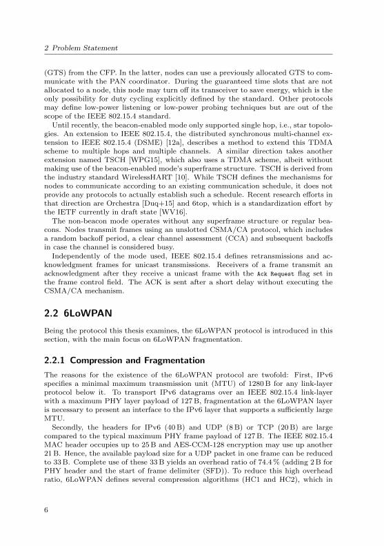
The reasons for the existence of the 6LoWPAN protocol are twofold: First, IPv6specifies a minimal maximum transmission unit (MTU) of 1280 B for any link-layerprotocol below it. To transport IPv6 datagrams over an IEEE 802.15.4 link-layerwith a maximum PHY layer payload of 127 B, fragmentation at the 6LoWPAN layeris necessary to present an interface to the IPv6 layer that supports a sufficiently largeMTU.
Secondly, the headers for IPv6 (40 B) and UDP (8 B) or TCP (20 B) are largecompared to the typical maximum PHY frame payload of 127 B. The IEEE 802.15.4MAC header occupies up to 25 B and AES-CCM-128 encryption may use up another21 B. Hence, the available payload size for a UDP packet in one frame can be reducedto 33 B. Complete use of these 33 B yields an overhead ratio of 74.4 % (adding 2 B forPHY header and the start of frame delimiter (SFD)). To reduce this high overheadratio, 6LoWPAN defines several compression algorithms (HC1 and HC2), which in
6

2.2 6LoWPAN
0 1 2 3 4 5 6 7 8 9 0 1 2 3 4 5 6 7 8 9 0 1 2 3 4 5 6 7 8 9 0 1
1 2 3
1 1 0 0 0 datagram size datagram tag
6LoWPAN FRAG 1 header
0 1 2 3 4 5 6 7 8 9 0 1 2 3 4 5 6 7 8 9 0 1 2 3 4 5 6 7 8 9 0 1
1 2 3
1 1 1 0 0 datagram size datagram tag
datagram offset
6LoWPAN FRAG N header
Figure 2.1: 6LoWPAN fragmentation headers
turn are updated by 6LoWPAN IPHC header compression (IPHC) [HT11]. Whilecompression is an important topic especially for small IPv6 datagrams with only ahandful of bytes payload, it is seen as a problem orthogonal to the performance of thefragmentation mechanism.
To implement fragmentation, 6LoWPAN defines two different fragmentation head-ers, one for a first fragment (FRAG 1) and a different one for any subsequent fragment(FRAG N; Fig. 2.1). Both include the uncompressed size of the IPv6 datagram anda tag to identify the datagram the fragment belongs to. The FRAG N header addi-tionally carries an offset field, which defines the position of the fragment within thewhole datagram given in a unit of 8 octets.
Provided with experience concerning the fragmentation of large data blocks whileworking at the iEZMesh project, I expected fragmentation to amplify existing prob-lems in multi-hop wireless mesh networks. iEZMesh was a project funded by theGerman government. One of the application requirements identified for the projectwas the collection of smart meter measurement tables sized 1 kB to 3 kB. With thelink-layer supporting frame sizes of 128 B, the preconditions are similar to those foundwith large fragmented IPv6 datagrams over IEEE 802.15.4. To satisfy the require-ments, we implemented a fragmentation mechanism at the transport layer, togetherwith an actual retransmission scheme for individual fragments based on negative ac-knowledgments. The evaluation of the performance yielded significant reliability is-sues for the large data blocks [Wei+14a], even in the presence of the mechanism forretransmissions.
Considering that the loss of a single fragment leads to the loss of a whole data-gram and the fact that typical wireless transmissions are inherently lossy due to theproperties of wireless channels, collisions and interference, I expect that 6LoWPANfragmentation is confronted with similar issues and that transmissions of large IPv6datagrams via 6LoWPAN may exhibit low reliability. Further it is to be expectedthat the impact of fragmentation increases with the number of fragments and thelength of a route. These considerations motivate the evaluation of the performanceof fragmentation and several forwarding strategies and the development of the newforwarding protocol 6LoOF, which are presented in this thesis.
7

2 Problem Statement
2.2.2 6LoWPAN Routing Schemes
With 6LoWPAN, routing in general can be performed at two different layers. First,a layer at the level 2.5 of the 6LoWPAN adaptation layer implements the routing.In that case, some mesh routing protocol has to emulate a full broadcast domainat the physical level for the IPv6 layer. This variant is called ımesh-under routing[HC08; Cho+09]. Thereby, link-local addresses and link-local multi-cast can easilybe used from an IPv6 layer perspective and IPv6-based protocols can theoreticallybe left unchanged. An example for this is the neighbor discovery protocol [Nar+07].Neighbor discovery makes extensive use of link-layer multicasts, which have to betranslated to flooding the mesh network. This means that the mesh routing protocolhas to provide potentially complex mechanisms to offer reliable operation over a multi-hop mesh network, which is far from trivial. Moreover, such mechanisms are alreadyavailable at the IPv6 network layer and have to be recreated for the layer 2.5 meshrouting [HC08].
The other possibility is to delegate routing decisions to the IPv6 layer: Every hopin a meshed 6LoWPAN network becomes an IPv6 routing hop. This routing schemeis called ıroute-over [HC08]. Using route-over has several implications. First, globalIPv6 addresses ([Nar+07]) have to be used, because IPv6 forbids routing of link-localaddresses. That makes the original HC1 and HC2 compression algorithms impracti-cal and is one reason for the introduction of the IPHC and 6LoWPAN next headercompression (NHC) [HT11]. With regard to fragmentation, route-over also meansthat datagrams – sticking to a strict separation of layers – have to be reassembled ateach intermediate hop of the 6LoWPAN mesh network, because fragmentation is thenhandled below the network layer.
With the creation of RPL [Win+12], a standardized routing protocol for low-powerand lossy networks at the IPv6 layer is available to be used with a route-over rout-ing scheme, which perfectly fits the usual demands on routing protocols for typical6LoWPAN wireless mesh networks. Considering the arguments, I decided to focus onthe evaluation of route-over, as it allows building a completely standardized protocolstack and avoids the awkward emulation of a single hop broadcast domain above alossy multi-hop wireless mesh network.
2.2.3 Basic Route-Over Forwarding Techniques
As described in Sect. 2.2.2, using the route-over routing scheme implies reassemblinga datagram at every intermediate node of the wireless mesh network. This is thefirst basic and most straightforward forwarding strategy and is called Assembly orAssembly mode throughout the thesis. During the whole process of reassembling thedatagram, all fragments have to be stored in some buffer, even at intermediate nodes,which are not concerned with the content of the datagram. Hence, for each datagramin transit, buffer space for the whole datagram has to be available. Considering typicalresource-constraint hardware for wireless sensor networks, this is a non-negligible issue.Furthermore, reassembling at every intermediate hop prevents pipelining of fragmentson longer (> 3) paths. Therefore, an unnecessary large end-to-end latency can beexpected (Fig. 2.2).
In contrast to this approach, which strictly preserves layer separation, a cross-layerapproach can be employed, which is called Direct or Direct mode in the remainder of
8

2.2 6LoWPAN
v1 l0 v2 l1 v3 l2 v4m1
m2
...
mnm1
m2
...
mnm1
m2
...
mn
(a) Assembly
v1 l0 v2 l1 v3 l2 v4
m1
m2
...
mn
m1
m2
...mn
m1
m2
...
mn
(b) Direct
Figure 2.2: Message flow in Assembly and Direct modes. The Direct mode has poten-tial for pipelining as well as an increased probability for collisions.
the thesis. For each incoming first fragment, the information necessary to identify andprocess subsequent fragments of the datagram is stored in a “virtual fragment buffer”.The buffer is called virtual, because it does not store the payload data the fragmentcarries, but only the metadata, i.e., information about progress and identity of thefragment. The fragment itself is immediately scheduled for transmission to the nexthop, which is queried directly from the IPv6 layer. This is always possible, becausethe IPv6 header does always fit the first fragment. Subsequent fragments then arematched against the entries in the virtual fragment buffer and routed along the samepath. Note that the Assembly mode also uses the same path, but the moment atwhich the routing decision is taken is different: with Assembly, it is the reception ofthe last fragment, with Direct, the reception of the first fragment.
Using the Direct mode, datagrams have only to be stored for reassembly at theirIPv6 destination (or the 6LoWPAN border router). Hence, it provides good potentialfor saving buffer space. Furthermore, pipelining on long paths becomes possible andthereby the overall latency can potentially be reduced. On the other hand, immediateforwarding also gives rise to self-interference. Fragments are prone to interfere withtheir predecessors, which have already advanced on the routing path. This can beespecially harmful at the node two hops farther down the path, because such a nodeusually will be a hidden-terminal. In this situation, the clear-channel assessmentpart of IEEE 802.15.4’s CSMA/CA algorithm is not able to prevent a collision. Thisincreased potential for collisions is also implied in Fig. 2.2.
2.2.4 Adjacent Protocols
The IPv6-based standardized protocol stack for resource constrained networks anddevices then could be the one shown in Fig. 2.3.
Above the described combination of a route-over 6LoWPAN adaption layer and theIPv6 network layer with RPL as routing protocol, the combination of UDP [Pos80]and CoAP [SHB14] is used at the transport and application layers.
9

2 Problem Statement
IEEE 802.15.4 PHY
IEEE 802.15.4 MAC
6LoWPAN
IPv6 RPL
UDP
CoAP
Application
Figure 2.3: Standard protocol stack for low-power lossy networks
CoAP is similar in spirit to Hypertext Transfer Protocol (HTTP) in defining ad-dressable resources as RESTful services. Additionally, it defines simple reliabilityfeatures, a basic congestion control mechanism and a binary representation to in-crease efficiency. Hence, it takes on some responsibilities of a transport layer. Currentstandardization and research efforts for CoAP focus, among others, on congestioncontrol [BGD15; Bet+15; JDK15] and blockwise CoAP transport [BS16]. The latterintroduces a mechanism to CoAP to split up large payloads into smaller blocks withthe target of avoiding to burden lower layers with “conversation state that is bettermanaged in the application layer”[BS16]. This includes 6LoWPAN fragmentation andaims at reducing the need for it and thereby is fundamentally different from the ap-proach presented in this thesis, which is to improve the performance of 6LoWPANfragmentation.
The RPL protocol [Win+12] defines a tree-based routing for low-power lossy net-works, such as wireless sensor networks or cyber-physical systems. Its main ideas arederived from the collection tree protocol [Gna+09]. It builds bi-directional routingtrees by two core mechanisms:
• Beacons called DIOs are used to form routes towards a single destination: theroot of the destination oriented directed acyclic graph (DODAG). The DIOspropagate from the DODAG root through the network governed by the Tricklealgorithm [Lev+11].
• Communication in the opposite direction is enabled by letting each node in thetree periodically send so-called DAOs to the DODAG root. That way, reverseroutes are installed either at each intermediate node (storing mode) or exclu-sively at the root, which uses source routing to transmit to arbitrary nodes.
RPL has been extensively evaluated [TOV10; HC11; YCI13; CMN14; KG14; Ise+15]and is emerging as the protocol of choice for static low power and lossy networks.
10

2.3 Applications
2.2.5 LFFR
Observing the same high probability for datagram losses when using fragmentationthat is discussed in Sect. 2.2.1, Thubert and Hui proposed a recovery mechanism for6LoWPAN fragments at the 6LoWPAN layer itself within an IETF draft [TH14]. Thisprotocol works with negative acknowledgments (NACKs), issued by the 6LoWPANmodule at the IPv6 destination of a datagram. Every NACK includes a bit vector,which marks the missing fragments. NACKs are “routed” back to the origin of thedatagram by using a reverse lookup and exchange of 6LoWPAN tag information thatis stored at the nodes and carried in the NACK, respectively.
The enhancements to 6LoWPAN forwarding of fragments presented in this thesiscould be combined with LLN fragment forwarding and recovery (LFFR) to furtherimprove the reliability of transmissions of large datagrams. However, at the time ofwriting, the draft [TH14] has expired and has not been renewed so far.
2.2.6 6TiSCH
As described in Sect. 2.1, TSCH extension to IEEE 802.15.4 does not define anymechanism to actually create and deploy a communication schedule for a network.The IETF 6TiSCH working group was founded to tackle this problem and recentlypublished a draft for the 6top protocol [WV16] and a general architecture of using6LoWPAN over TSCH [Thu15].
2.3 Applications
6LoWPAN is mainly designed with the goal of transporting small datagrams using theIEEE 802.15.4 link layer. Its compression mechanisms reduce the overhead caused byIPv6 and upper layer protocol headers and for small payloads achieve to stuff an IPv6datagram into a single IEEE 802.15.4 frame. However, given the minimum maximumMTU of 1280 B defined for IPv6, datagrams of this size are completely legal and there-fore – I argue – will be used by future applications and should achieve an acceptableperformance. Furthermore, there are already several applications from the field ofwireless sensor networks which exhibit traffic patterns involving the transmission oflarge data objects.
A part of the advanced metering infrastructure, which in turn is a part of the effortstowards smart grids, is smart metering, i.e., the automated report of consumptiondata of customers to utilities. While in past days, this communication was restrictedto the consumption values for a whole year, the realization of smart grids demandsfor detailed load profiles with a much finer temporal granularity. Such can comein sizes from several hundred bytes to several kibibytes, depending on the type ofthe meter. One option for the transport of such data are wireless mesh networks.Within the iEZMesh project [Wei+14a], requirements to transport load profiles ofup to 3 KiB every 15 min were identified. While the proposed solution included aproprietary network protocol stack, a realization of such requirements with an IPv6stack including 6LoWPAN is thinkable.
Another application scenario that potentially produces a large amount of data isstructural health monitoring of buildings and structures like bridges, which has al-ready triggered research efforts on transport protocols for large data objects [Pae+05;
11

2 Problem Statement
Kim+07b; Kim+07a; PG10; Kur+12]. For these applications, data is created withhigh frequencies and sent to a sink for offline analysis. Approaches exists to reduce thedata volume by shifting the computational effort to the sensor nodes and exchangingpartial results among nodes [Boc+11], but have been tested only with very simple one-hop topologies. Similar with regard to the amount of data created are applications forearthquake, volcano monitoring [Wer+06; Suz+07] and image processing applicationsfor, e.g., environmental monitoring [Ko+10].
In general, wherever “large” – in the sense of not fitting a IEEE 802.15.4 frame –data has to be transferred to a data sink, 6LoWPAN fragmentation has to be applied.
2.4 Energy Availability
For many applications in the field of wireless sensor networks or the IoT, a part ofthe participating nodes are powered by batteries or energy harvesters that do notyield enough for the node to be in an “always-on” state. A large number of researchefforts for wireless sensor networks has therefore been directed at the development oflow-power protocols, aiming at the extension of the lifetime of individual nodes or thewhole network [MLT08; Bue+06]
Current available IEEE 802.15.4 transceivers consume a nearly equal amount ofpower in RX and TX state. For example, the Atmel AT86RF231 consumes 12.3 mAin RX and 14 mA in TX states according to the datasheet [14]. Put into sleep mode,on the other hand, most current transceivers draw current less than 1 µA. There-fore, to effectively reduce energy consumption, transceivers have to be duty cycled.Dominant techniques to achieve low duty cycles are low-power listening [Bue+06] andlow-power probing [MLT08]. The former is usually implemented by either repeatingthe transmission of a frame multiple times (until the receiver wakes up and notices theactivity) or by using long preambles. The latter takes an opposite approach: nodesready to receive send a short probing frame to signal their readiness and senders stayactive and listen for such a probe if they have something to send. Both approaches aremainly applicable for low-data rate applications – if nodes have to transmit continu-ously, the reduction in energy conservation is decreased. Also, low-power mechanismstrade savings in energy consumption with increased latency and decreased throughputdue to waiting for other nodes’ active phases.
To the best of my knowledge, there is no low-power listening or probing mechanismstandardized for IEEE 802.15.4. According to [11a], nodes that act as routers in non-beacon enabled PANs have to be always on, because they can not know when a framewill be transmitted to them [Wat+16]. In beacon-enabled networks (Sect. 2.1), nodescan sleep in the contention free period during slots unused by them.
Various energy harvesting technologies have been proposed to allow for sustainableoperation of sensor nodes [SK11]. Different technologies have been evaluated, rangingfrom photovoltaics over thermoelectric to piezoelectric. Harvesting solutions can befurther differentiated by the type of storage system they use. Typically, at least onerechargeable battery is used. Additionally, supercapacitors, which allow for a near-infinite number of recharge cycles are integrated as primary storage to prevent manyunnecessary shallow recharge cycles of the main battery [Ren13].
Most existing solutions aim at supporting nodes that are duty-cycled. However,with solar panels of a given dimension and a suitable environment, it is possible to
12

2.5 Goals of Evaluation
provide enough power for perpetual operation of always-on nodes. This has beendemonstrated in a field test during the HelioMesh project, where solar panels wereused to provide the energy for the motors of heliostats as well as an attached sensornode [Unt14].
Current IEEE 802.15.4 transceivers, e.g., the Atmel ATmega256RFR2, offer a lowpower RX state, cutting the current consumption by a factor of two. While theconcrete working details of this mode of operation of the mentioned transceiver are notpublished by Atmel, I suspect that this mode implements a straightforward 50 % dutycycling scheme at the level of IEEE 802.15.4 symbols that activates the transceiver assoon as the preamble is received. It is claimed that activation of this mode decreasesthe receiver sensitivity by about 3 dB. While such transceiver supported energy savingmodes can in their current state not be expected to replace more advanced low-powerlistening or probing techniques, they can help to reduce the overall energy consumptionof routing nodes to allow for smaller dimensions of harvesters.
2.5 Goals of Evaluation
As stated in Sect. 2.2.1, the main goal of this dissertation is to evaluate the perfor-mance of 6LoWPAN fragmentation and the different forwarding strategies for largeIPv6 datagrams. Furthermore, techniques to improve the situation are to be devel-oped and their performance compared to the existing approaches. This is done forIEEE 802.15.4/6LoWPAN networks that use the non-beacon enabled mode of oper-ation and assume that at least routing nodes within a network are always on. Thereare several reasons for this decision:
• The sending of large datagrams implies comparatively high data rates. Forthose, low-power listening or probing techniques are not well suited.
• At the time of writing, there is no standardized low-power mode of operationfor IEEE 802.15.4, other than nodes sleeping in the CFP. The beacon-enabledmodes, however, are not standardized for multi-hop operation until very recentlywith the proposal of DSME. Aiming at a fully standardized protocol stack, Idecided to go for the unslotted operation with always-on nodes.
• Of the potential applications introduced in Sect. 2.3, smart metering can employseveral grid-powered nodes (at electricity meters) and other applications (envi-ronmental, structural monitoring) are eligible for a backbone of routing nodeswith generously dimensioned harvesting solutions.
Recent TDMA-based extensions to IEEE 802.15.4 (DSME, IPv6 over the TSCHmode of IEEE 802.15.4e (6tisch)) are promising alternatives to also provide good per-formance for large fragmented datagrams but are not considered in this dissertation.They yet have to prove that the proposed scheduling solutions work in large networksand with larger payloads [Wat+16].
A typical application scenario may employ the IETF stack described in Sect. 2.2.4.Fig. 2.4 shows a topology similar to those obtained from a testbed in the iEZMeshproject. While during the project proprietary protocols were used, the network couldalso utilize an IETF stack and contain a number of always-on nodes that form a
13

2 Problem Statement
Figure 2.4: Application scenario with routing (blue) and leaf nodes (gray). The topol-ogy is similar to the routing topology observed during a field test in theiEZMesh smart metering project. The central node represents the wirelesssink.
RPL routing tree, complemented by a number of RPL leaf nodes that do not activelyparticipate in forwarding of data. Different from the routing nodes, these leaf nodesare expected to sleep most of the time and become active only when they have datato send. The extensions to IPv6 neighbor discovery for 6LoWPAN defines messageformats and options to existing message formats to cope with such leaf nodes.
14
3 Analytic Model for 6LoWPAN-FragmentedForwarding
This chapter introduces an extension to an existing analytical model for 6LoWPAN-fragmented transmissions of IPv6 datagrams.
3.1 Motivation and State of The Art
This section discusses the motivation for the creation of the model and provides anoverview on existing related work.
3.1.1 Motivation
There are two major reasons to analytically model the process of 6LoWPAN fragmentforwarding. First, for a fragmented datagram to be received successfully, all fragmentsbelonging to that datagram have to be received successfully. It is intuitively clear thatincreasing the size of the datagram and hence the number of fragments decreases theprobability for success on lossy wireless links, especially if transmissions via multiplehops are considered. Instead of relying on intuition, an analytical model can help toquantify this issue.
Secondly, between the two basic forwarding modes introduced in Sect. 2.2.3, thereis a major difference in how they handle fragments of datagrams that get lost duringreception. By definition, the Assembly mode will never forward any fragments of anincompletely received datagram: if any fragment gets lost, the datagram will not besent to the IP layer and therefore will not be routed further. The Direct mode, onthe other hand, forwards fragments as soon as they arrive. Thus, even if a datagramis lost early on the path, some of its fragments may propagate through the networkwithout adding to the overall goodput. To quantify the magnitude of this effect isanother motivation for creating a model.
Finally, there are two diametrically different approaches to handle the situation ofa failed transmission of a fragment:
1. Assume the fragment and therefore the whole datagram is lost and in conse-quence, abort transmission of the whole datagram – this is called non-persistingstrategy in the remainder of the thesis.
2. Continue sending fragments even after a transmission failure of a fragment andalso continue sending subsequent fragments if a fragment is missing. In theformer case, there is a probability that not the fragment, but the ACK waslost and therefore the datagram is not lost as a whole – this is called persistingstrategy in the remainder of the thesis.
15

3 Analytic Model for 6LoWPAN-Fragmented Forwarding
By means of an analytical model, these different approaches can be evaluated. Iexpect the persisting strategy to increase the success rate of datagrams marginallyand at the same time to exhibit a comparatively large number of sent frames dueto failed datagrams whose remains continue to propagate through the network. Forthis reason, the persisting strategy is not ideal for route-over schemes without anyend-to-end recovery mechanism of fragments.
3.1.2 State of the Art
Several research efforts have been undertaken to analyze the performance of 6LoWPANfragmentation over IEEE 802.15.4 networks using analytical models.
The model presented in Section 3.2 is derived from the model of Ayadi et al., whoanalyzed the efficiency of different TCP segment sizes ([AMR11]). Their model isbased on bit error probabilitys (BEPs) that are stochastically independent. Frag-mented datagrams, link-layer retransmissions, forward error correction and multiplehops are modeled. Typical effects of wireless channels like collisions, quality degrada-tion or (self-) interference, on the other hand, are not captured by a channel modelbased solely on BEPs. The persistent strategy is used in case of failures. For a givenset of input parameters, a datagram success rate and the expected number of bits sentcan be determined with their model.
Subsequent work of Ayadi et al. [Aya+11] reuses their basic model and extendit to assess the effectiveness of LLN Fragment Forwarding and Recovery (LFFR),which is described within an internet draft of the IETF ROLL working group [TH14]and has expired at the time of writing. LFFR defines a layer-2.5 transport protocolfor 6LoWPAN fragments, which enables the 6LoWPAN layer to retransmit individualfragments triggered by negative acknowledgments from the receiver. For this scenario,their assumption that nodes continue sending fragments although a former fragmenthas failed, is a reasonable one.
A different approach that tries to take into account collisions and is not specificallytailored to typical 6LoWPAN scenarios has been followed by Di Marco et al. [Di +12],which is in turn based on [Bia06]. Their models are based on Markov chains and modelthe transmission of frames over multiple hops by state transitions, taking into accountclear-channel assessment, backoffs and link-layer retries. Output values of this modelare latency, energy consumption (derived from a node’s state) and reliability. Thisapproach is potentially much more accurate than a model based solely on bit-errors,which neglects any potential and impacts of collisions between frames. However, theirmodel is based on average rates of arrival and therefore can not capture the effect that alarge number of frames arrive at a node simultaneously, as it is typically the case usingfragmentation. The effect of a thus filled transmission queue is an increased probabilityfor self-induced interference, which is neglected by the model (Sect. 2.2.3). This modelwas also extended by Meier and Turau, who added the handling of downstream traffic[MT15]. The extended model also recognizes the possibility for acknowledgments withdata frames and with each other and take into account the increased probability ofcollisions after a collision (because two nodes start transmitting at the same time).
An analytical model that does take into account 6LoWPAN fragmentation andtransmission of large datagrams was introduced by Ludovici, Di Marco, Calverasand Johansson [Lud+14]. It is used to compare the performance of CoAP’s block-wise transfer [BS16], which is still being standardized at the time of writing, and
16

3.2 Model
6LoWPAN fragmentation. Their results suggest that “6LoWPAN fragmentation out-performs CoAP blockwise transfer with regard to latency independently from theupdate generation rate and the number of nodes”. CoAP blockwise transfer exhibitsa higher reliability in congested traffic scenarios. The model is restricted to single-hopscenarios and therefore not applicable to the multi-hop scenarios considered in thisthesis.
3.2 Model
The model is an extension of the one presented by Ayadi et al. and follows thesame approach taken to derive probabilities and expectation values presented in theirpaper [AMR11]. It calculates the number of expected bits sent and the frame successprobability (FSP) depending on link BEPs, the number of link-layer attempts anda forward error correction (FEC), i.e., a redundancy ratio which yields a numberof correctable bit errors. It is assumed that bit errors are independent of each other.Additionally, it is assumed that duplicates are detected by the 6LoWPAN layer, whichis realistic as it needs to keep track of the state of fragmented datagrams anyway.
As described in Sect. 3.1.2, the major difference between the existing model andthe extension is the handling of failures and partial failures. While Ayadi et al. let asender always send all fragments, I assume that a sender gives up on a datagram in caseof a failure or partial failure. I also consider both forwarding techniques introducedin Sect. 2.2.3 in that context: Assembly and Direct mode. I implemented both theextended model and the original model of Ayadi. The latter was slightly modified toget comparable resulting quantities. Consistent with Sect. 3.1.1, the extended modelfor Assembly and Direct mode is referred to as non-persisting model, the originalmodel is referred to as persisting model in the remainder of this thesis.
3.2.1 Link-Layer Model
At the link layer, three different outcomes of a transmission are defined:
• The transmission failed (probability pf,k)
• The transmission partially failed, i.e., the frame arrived but the ACK was neverreceived (probability pp,k)
• The transmission was successful, frame and ACK arrived (probability ps,k)
At their hearts, both models are based on the pe,k of a link k. In case of the occurrenceof an uncorrectable bit error, the transmission is considered unsuccessful, yielding theintroduced probabilities as
pf,k = 1−c∑i=0
(LF
i
)pie,k(1− pe,k)LF−i (3.1)
pp,k = (1− pf,k)(1− (1− pe,k)LA ) (3.2)
ps,k = (1− pf,k)(1− pe,k)LA = 1− (pp,k + pf,k) (3.3)
17

3 Analytic Model for 6LoWPAN-Fragmented Forwarding
with the number of correctable bit errors c and the link layer frame sizes LF and LA
for a data and Ack frame, respectively. I stick with the approach from [AMR11] tomodel FEC only for the data packet, not the acknowledgment. While the model itselfthereby regards the possibility of a FEC mechanism, for the evaluation in this chapterI consider c = 0 and do not go into further details about the derivation of the numberof fragments for a given datagram size.
Based on those basic formulas, the probabilities for success, partial failure andfailure after r send attempts can be derived as
P s,k =
r∑j=1
ps,k(1− ps,k)j−1 =
r∑j=1
ps,k
j−1∑i=0
(j − 1
i
)pip,kp
j−1−if,k (3.4)
Pp,k = (pp,k + pf,k)r − prf,k =
r∑j=1
(rj
)pjp,kp
r−jf,k (3.5)
P f,k = prf,k (3.6)
and the conditional expectation value for the number of sent bits in each case canthen be derived by enumerating all possible outcomes after r attempts as
Hs,k =1
P s,k
r∑j=1
ps,k
j−1∑i=0
(j − 1
i
)pip,kp
j−1−if,k (jLF + (i+ 1)LA)
(3.7)
Hp,k =1
Pp,k
(r∑i=1
(ri
)pip,kp
r−if,k (rLF + iLA)
)(3.8)
Hf,k =1
P f,krLFP f,k = rLF (3.9)
Hsp,k =1
1− P f,k
(Pp,kHp,k + P s,kHs,k
)(3.10)
where Hy,k is the expected number of bits sent in case of success, partial failure orfailure on link k, with the corresponding probability Py,k. In addition to the valuesfor the three possible outcomes, I define as Hsp,k the expected number of bits sent incase of a success or a partial failure. The formulas presented so far are basically thoseintroduced by Ayadi et al. [AMR11], extended by an index to identify a certain hopand a slight rearrangement due to the different results which partial failures producein the multi-hop model.
3.2.2 Multi-Hop Model
We define the route the fragments have to traverse as a series of hops (wireless links)k numbered from 1 to n. Moving to this multiple hop, multiple fragment scenario, weget for the probability of success and failure of a datagram consisting of m fragments
18
3.2 Model
Ps and Pf , independent of the actual forwarding mode:
Ps(h0, h,m) =
h∏k=h0
(Pm−1s,k (P s,k + Pp,k)), (3.11)
Pf(h0, h,m) =
h∑k=h0
Ps(h0, k − 1,m)
(m−1∑x=1
Px−1s,k Pp,k +
m∑x=1
Px−1s,k P f,k
), (3.12)
where h0 is the index of the first hop, h the index the final hop and m the number offragments sent. For example, Ps(1, 8, 10) is the probability of success for a datagramfragmented into 10 fragments on a route of 8 hops, the bit error probabilities pe,k
have to be defined accordingly for each link. For the last fragment sent, a partialfailure is sufficient, because it does not matter whether the sender would give up onthe datagram afterwards.
With the Assembly mode, no fragments of a failed datagram are propagated anyfurther after the first fragment failure. The expected number of bits sent in Assemblymode EA therefore is
EA(h0, h,m) = Ps(h0, h,m)EAs (h0, h,m) + Pf(h0, h,m)EA
f (h0, h,m) (3.13)
EAs (h0, h,m) =
h∑i=h0
((m− 1)Hs,i +Hsp,i) (3.14)
EAf (h0, h,m) =
1
Pf(h0, h,m)
h∑k=h0
Ps(h0, k − 1,m)×
(m−1∑x=1
((x− 1)Hs,k +Hp,k + EAs (h0, k − 1,m))Px−1
s,k Pp,k
+
m∑x=1
((x− 1)Hs,k +Hf,k + EAs (h0, k − 1,m))Px−1
s,k P f,k
)(3.15)
where EAs and EA
f are the conditional expectation values of the number of bits sentin case of success and failure, respectively.
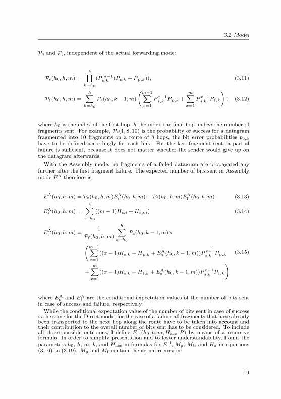
While the conditional expectation value of the number of bits sent in case of successis the same for the Direct mode, for the case of a failure all fragments that have alreadybeen transported to the next hop along the route have to be taken into account andtheir contribution to the overall number of bits sent has to be considered. To includeall those possible outcomes, I define ED(h0, h,m,Hacc, P ) by means of a recursiveformula. In order to simplify presentation and to foster understandability, I omit theparameters h0, h, m, k, and Hacc in formulas for ED, Mp, Mf , and Hz in equations(3.16) to (3.19). Mp and Mf contain the actual recursion:
19
3 Analytic Model for 6LoWPAN-Fragmented Forwarding
vi vi+1 vi+2
0
0 X1
0 X1 X2
0 X1 X2 X3
···
0
0 X1
0 X1 X2
0 X1 X2 X
0
0 X1
0 X1 X
· · ·
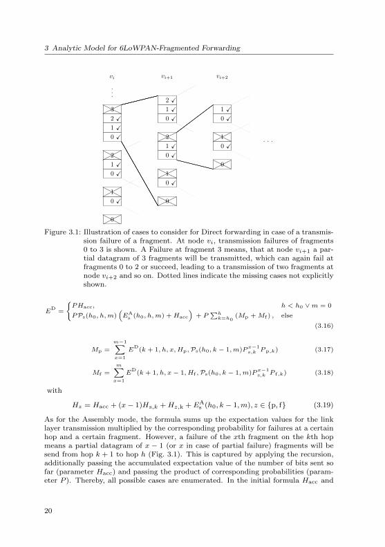
Figure 3.1: Illustration of cases to consider for Direct forwarding in case of a transmis-sion failure of a fragment. At node vi, transmission failures of fragments0 to 3 is shown. A Failure at fragment 3 means, that at node vi+1 a par-tial datagram of 3 fragments will be transmitted, which can again fail atfragments 0 to 2 or succeed, leading to a transmission of two fragments atnode vi+2 and so on. Dotted lines indicate the missing cases not explicitlyshown.
ED
=
{PHacc, h < h0 ∨m = 0
PPs(h0, h,m)(EA
s (h0, h,m) +Hacc
)+ P
∑hk=h0
(Mp +Mf ) , else
(3.16)
Mp =
m−1∑x=1
ED
(k + 1, h, x,Hp,Ps(h0, k − 1,m)Px−1s,k Pp,k) (3.17)
Mf =
m∑x=1
ED
(k + 1, h, x− 1, Hf ,Ps(h0, k − 1,m)Px−1s,k P f,k) (3.18)
with
Hz = Hacc + (x− 1)Hs,k +Hz,k + EAs (h0, k − 1,m), z ∈ {p, f} (3.19)
As for the Assembly mode, the formula sums up the expectation values for the linklayer transmission multiplied by the corresponding probability for failures at a certainhop and a certain fragment. However, a failure of the xth fragment on the kth hopmeans a partial datagram of x − 1 (or x in case of partial failure) fragments will besend from hop k + 1 to hop h (Fig. 3.1). This is captured by applying the recursion,additionally passing the accumulated expectation value of the number of bits sent sofar (parameter Hacc) and passing the product of corresponding probabilities (param-eter P ). Thereby, all possible cases are enumerated. In the initial formula Hacc and
20
3.3 Evaluation
Table 3.1: Default parameter values
Parameter Value Parameter Valuer 5 c 0h0 1 h 8m 12 pe,k 2.4244× 10⁻⁴
P are set to 0 and 1, respectively. For example, the expected number of bits sent tosend 10 fragments via hops 1 to 5 then can be obtained by ED(1, 5, 10, 0, 1).
3.3 Evaluation
To evaluate the impact of the different forwarding techniques, the model is fed withdifferent scenarios varying BEP, denoted as pe , number of link-layer attempts, numberof hops and number of fragments. The potential use of FEC (c > 0) is not evaluatedfurther. For all scenarios, LF = 119 B is used, including 11 B MAC header and 2 BPHY header, leaving an 802.15.4 payload of 106 B. A link-layer acknowledgment of 7 Bsize is assumed. Unless specified differently, I set the non-varying input parametersto the values shown in Table 3.1. Besides the overall probability of success for atransmission, the model’s main output metric is the expected number of bits sent,which indicates the amount of energy used for transmission as well as the overall trafficload produced. In the following, additional subscripts P and NP indicate persistingand non-persisting forwarding strategy (see Section 3.2), respectively.
While the model allows for a different BEP to be assigned to each link, for theevaluation presented here I used equal rates for all links. To calculate results, themodel was implemented as a Mathematica module. Results were calculated and com-pared with different guarantees for precision, so that numerical instabilities biasingthe results can be ruled out.
3.3.1 Persistent vs. Non-Persistent
First, the difference between persisting and non-persisting forwarding is assessed bycomparing the output from the original model with the extended version. On the onehand, I expected the probability of success for the persisting strategy to be slightlyhigher than for the Assembly and non-persisting Direct mode, because partial failureson a link are counted as an overall success with regard to the transmission of a frag-ment. On the other hand, the expected number of bits sent should be significantlyhigher for the persisting approach, as even in the case of a failure a sender continuessending all remaining fragments. Figure 3.2 shows a comparison of the two strategiesfor different values of the BEP. Subscripts P and NP denote quantities for persistingand non-persisting strategy, respectively.
While the effect of persisting on the probability of success is comparatively small –for the shown BER values it stays below 0.03 –, the impact on the expected numberof bits sent is significant. Note also that in a real network, failures are likely causedby interfering transmissions of other nodes. Continuing transmissions after a failuremay therefore also impact other, not-yet-failed, transmissions. In the light of those
21

3 Analytic Model for 6LoWPAN-Fragmented Forwarding
0.8
0.85
0.9
0.95
1
Pro
babi
lity
ofSu
cces
s
Ps,P
Ps,NP
10−4 10−3.9 10−3.8 10−3.7 10−3.6 10−3.5
1
1.5
2
2.5
pe,k
Rat
ioof
expec
ted
num
ber
ofbi
tsse
nt
EDNP/EA
NP
EP/EANP
Figure 3.2: Comparison of the ratios of the number of expected bits sent (left y-axis)and the probability of success (right y-axis) for persisting (subscript P)and non-persisting (subscript NP) approaches against the BEP (pe ).
results, using such a persisting strategy for the given scenario is considered inadvis-able. Therefore, in the remaining evaluation, the focus is shifted to the non-persistingmethod.
3.3.2 Multi-Hop Transmissions
Figure 3.3a indicates the impact of the number of hops and retransmissions for ap-plying 6LoWPAN fragmentation: It shows the probability of successful transmission
1 2 3 4 5 6 7 8
0.4
0.6
0.8
1
Number of Hops h
Ps,N
P
r=3r=4r=5r=6
(a) Probability of success Ps,NP againstnumber of hops for different maxi-mum numbers of retransmissions
2 4 6 8
1
1.1
1.2
Number of Hops h
ED NP
Em
in
r=3r=4r=5r=6
(b) Normalized expectation value of num-
ber of bits sent EDNP/Emin against
number of hops for different maximumnumbers of retransmissions
Figure 3.3: Influence of number of hops and the maximum number of retransmissions,non-persistent mode
22

3.3 Evaluation
10−4 10−3 10−20
0.5
1
1.5
2
2.5
pe,k
Rat
ioof
expec
ted
num
ber
ofbi
ts,pr
obab
ility
ofsu
cces
s
EDNP/EA
NP
(EDf,NP − EA
f,NP)/Emin (failure case)Ps,NP
Figure 3.4: Non-persisting mode; Ratio of expected number of bits sent in Direct(ED
NP) and Assembly mode (EDNP), together with overall probability of
success and the difference in bits for the number of bits sent in case offailure for both modes, normalized by Emin, against BEP.
Ps,NP of a large, 6LoWPAN-fragmented datagram for one to eight hops and for dif-ferent maximum numbers of link-layer retransmissions r. It can be seen that Ps,NP
decreases for an increasing number of hops. The effect is more strongly pronouncedfor smaller values of r. For the given pe and r = 3 (the default value defined inthe IEEE 802.15.4 standard), Ps,NP drops below 0.4 at eight hops. A higher max.number of link-layer retransmissions counters this effect: for r = 6, Ps,NP only dropsa few percent below 1.
Additionally considering the expected number of bits sent (normalized by the mini-mum number of bits needed for the complete transmission), shown in Fig. 3.3b, it canbe seen that the improved probability for success is bought by increasing the numberof frames sent. For r = 6, more than 25 % more bits than for a “perfect” run are sent.The increased number of bits does not have any effect on the probability of successin the presented model. In a real network, this increased traffic volume may increasethe probability of collisions and therefore potentially reduce the positive effect on theoverall probability of success of increasing r. Still, the result indicate that a largernumber of retransmissions in general increases the probability of success.
3.3.3 Additional Bits in Direct Mode
Figure 3.4 shows the ratio of expectation values of bits sent for Direct and Assem-bly modes (ED
NP/EANP) along with the overall probability for success of the whole
datagram Ps,NP, which is the same for both forwarding techniques. For success ratesapproaching 1 and 0, the difference between the expected number of bits sent in Di-rect and Assembly forwarding modes approaches zero. However, for a probability ofsuccess of 0.81 a ratio of 1.04 can be observed, i.e., a 4 % increase compared to the
23
3 Analytic Model for 6LoWPAN-Fragmented Forwarding
0 2 4 6 8 10 120.8
0.85
0.9
0.95
1
Number of fragments m
Ps,N
P
pe,k = 0.00049pe,k = 0.00035pe,k = 0.00024
(a) Probability of success
0 2 4 6 8 10 12
0
0.1
0.2
Number of Fragments m
ED f,N
P−
EA f,N
PE
min
pe,k = 0.00024
(b) Normalized difference between Directand Assembly mode
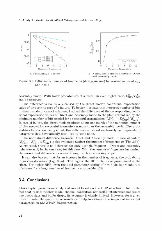
Figure 3.5: Influence of number of fragments (datagram size) for several values of pe,k
and r = 5
Assembly mode. With lower probabilities of success, an even higher ratio EDNP/E
ANP
can be observed.
This difference is exclusively caused by the direct mode’s conditional expectationvalue of bits sent in case of a failure. To better illustrate this increased number of bitsin direct mode in case of a failure, I added the difference of the corresponding condi-tional expectation values of Direct and Assembly mode to the plot, normalized by theminimum number of bits needed for a successful transmission ((ED
f,NP−EAf,NP)/Emin).
In case of failure, the direct mode produces about one fourth of the minimum numberof bits needed for successful transmission more than the Assembly mode. The prob-abilities for success being equal, this difference is caused exclusively by fragments ofdatagrams that have already been lost at some node.
The normalized difference between Direct and Assembly mode in case of failure(ED
f,NP−EAf,NP)/Emin) is also evaluated against the number of fragmentsm (Fig. 3.5b).
As expected, there is no difference for only a single fragment – Direct and Assemblybehave exactly in the same way for this case. With the number of fragments increasing,the normalized difference increases, though with a decreasing slope.
It can also be seen that for an increase in the number of fragments, the probabilityof success decreases (Fig. 3.5a). The higher the BEP, the more pronounced is theeffect. For higher BEP, even the used parameter setting of r = 5 yields probabilitiesof success for a large number of fragments approaching 0.8.
3.4 Conclusions
This chapter presents an analytical model based on the BEP of a link. Due to thefact that it does neither model channel contention nor (self-) interference nor issueslike queue sizes and buffer drops, its accuracy is clearly limited. However, for a givenbit-error rate, the quantitative results can help to estimate the impact of importantparameters on 6LoWPAN-fragmentation.
24

3.4 Conclusions
Given a significant probability for errors, which is a usual case for real wirelessnetworks, it shows that the combination of a large number of fragments and and a largenumber of hops dramatically decreases the overall probability of success of a datagramtransmission and is thereby consistent with the my expectation. Increasing the numberof retries counters the effect, albeit at the cost of additional frames sent. If thoseadditional frames can actually have a negative impact on the overall datagram successrate is evaluated by simulation and testbed experiments (Chapter 5 and Chapter 7).
It could also be seen, that a persisting strategy on the one hand increases theprobability of success slightly, but on the other hand produces a large number ofadditional fragments in the network in comparison to the non-persisting strategy.Furthermore, it was shown that in case of failure, the Direct mode creates about25 % more fragments than the Assembly mode. These additional fragments do notcontribute to the goodput of the network. However, the share of these fragments inthe total number of fragments is small for datagram success rates of more than 80 %and therefore is not expected to have a significant influence on the performance inreal networks.
25


4 Simulation Model and Environment
The proposed enhancements to a 6LoWPAN implementation (Sect. 5.2.1), including6LoOF (Sect. 8), are evaluated by simulations and testbed experiments. Simulationswere mainly used to perform parameter studies that were too expensive in terms oftime for testbed experiments. To obtain meaningful results, the model used by thesimulation environment has to reflect properties of the real world that have an impacton the behavior of the simulation. This means that a reasonably accurate modelfor the IEEE 802.15.4 physical layer operating in the 2.4 GHz ISM band has to beimplemented. Furthermore, the simulation model has to be validated [WGG10]. Thischapter introduces the used simulation tools and modeling frameworks (Sect. 4.1). Itfurthermore discusses methods to model the physical layer of wireless transmissionsand describes the one taken for this thesis (Sect. 4.2). Lastly the approach taken toproduce simulation scenarios from measured data to validate the simulation model(Sect. 4.3) is described.
4.1 Frameworks and Tools
This section introduces the simulation environment and frameworks that were utilizedto obtain the measurement data.
4.1.1 OMNeT++
The OMNeT++ simulation framework [Var99; Var+01; VH08] has been around since1997. While being a generic “discrete event simulation environment”, it is mainly usedfor simulation of wired, wireless and mobile communication networks. OMNeT++itself does not contain any simulation models. Support for a large number of internetprotocols and more recently also for an increasing number of wireless protocols andmodels for the physical layer is provided by the INET model suite.
OMNeT++ is based on modules, which communicate with each other by passingmessages to gates. The simulation model is then defined by connecting the gates be-tween modules and the C++-implementation of the individual modules. By adheringto this general concept, a loose coupling of reusable components can be realized.
Various tools are available for debugging, verification and analysis. These reachfrom “watching” network packets in slow motion within the provided graphical userinterface over detailed event logs capturing all message passing events to statisticsrecording and graphical analysis of those.
I chose OMNeT++ as simulation environment, because of its openness for aca-demic purposes, the described modular design and availability of several extensionsfor advanced modeling of the physical layer. Furthermore, another open and popu-lar simulation environment, ns3 [RH10], was not as well developed at the time thedecision was made.
27

4 Simulation Model and Environment
4.1.2 MiXiM
One thing lacking from the OMNeT++/INET-combination until recently, were sophis-ticated models for the physical layer. Among the available solutions providing thosewas the MiXiM framework [Kop+08; Wes+09], which also contains models for mobil-ity, batteries and mac protocols. Castalia [PTB10] is another simulator, which is basedon OMNeT++’s event engine and which is focused on PHY layer models for wirelesssensor and body area networks. For this thesis and CometOS (Sect. 4.1.3), MiXiMwas chosen, because it easily integrates into existing OMNeT++ projects and pro-vides sophisticated means to provide physical models as well as a basic IEEE 802.15.4link layer implementation. At the time of writing, both the original MiXiM projectand Castalia seem to be abandoned, but parts of MiXiM are being refactored andintegrated into INET.
MiXiM’s physical layer simulation is realized by a customizable (by inheritance)BasePhyLayer module. This module is responsible for the transmission and reception ofAirFrames. When transmitting an AirFrame, it is passed to all potential receivers andnodes within interference range of the sender. The actual receivers are determinedby a ConnectionManager to avoid expensive calculations for nodes that are not withininterference range. Reception then comprises three steps:
• Pass the AirFrame to a ChannelInfo object, which keeps track of all incomingframes for a node.
• Pass the Signal to all active analogueModels for processing
• Pass the AirFrame to a Decider.
The latter two actions offer entry points for customization. First, the type of theDecider can be configured and it is also possible to create new Deciders by creating a newsubclass. The Signal, which is attached to the AirFrame, is processed by analogueModels.A Signal consists of information about the signal strength (depending on the node’stransmission power) and information about its temporal extent and its spatial origin.Each analogueModel calculates an attenuation and attaches it to the Signal, resulting ina Mapping (a matrix-like data structure) that represents signal strength at the receivingnode for different points in time and optionally different frequencies.
The actual decision about whether a frame is received correctly then is delegated tothe decider by calling it at least at the beginning and end of a frame transmission. Themore sophisticated Deciders bundled with MiXiM check if the strength of an incomingsignal is strong enough to be received at all and if another signal is already beingreceived (in which case, the new signal is not received). “Strong enough” here meansthat during the SFD, the SINR of the incoming signal does not cause a bit error.To calculate the SINR, all incoming and processed (attenuated by the analogueModels)Signals stored in the ChannelInfo object are considered. At the end of a frame reception,the decider is called again and determines if a bit error has occurred within the frame.The calculation of bit error probability depends on the used modulation techniqueand the SINR. The MiXiM-provided Deciders then either pass the received frame orthe information that the frame was dropped to the connected MAC module.
Thereby, MiXiM provides an simulation of the physical layer at the bit level [WGG10].It is also able to model collisions of frames by means of the ChannelInfo module.
28

4.2 Physical Layer Model
4.1.3 CometOS
The protocols evaluated in this thesis are implemented in CometOS. CometOS is –similar to OMNeT++ – based on modules that exchange messages via gates. Thissimilarity is deliberate. Several adapter classes enable modules written for CometOSto be executable as OMNeT++ simulations. Thereby, CometOS aims to provide aframework for rapid protocol development and verification.
In addition to the simulation capabilities via OMNeT++, CometOS provides acore framework that provides modules, gates and message passing, as well as a non-preemptive scheduler for arbitrary platforms. A platform-dependent implementationof a very slim platform abstraction layer (PAL) is required for the core functions towork. Additional PALs define interfaces for typical communication buses (UART,TWI, SPI), low-level IO (GPIOs), watchdog timer, persistent memory and a linklayer for wireless communication. The latter is used by a platform-independent mod-ule named MacAbstractionLayer, which offers a unified interface for protocol stacksrunning within an OMNeT++ simulation or a specific hardware platform.
We chose the link layer as level of abstraction between simulation and hardware-based platforms, because several transceivers already support extended operationmodes, which implement the complete CSMA/CA protocol and automatic acknowl-edgments and retransmissions in hardware and therefore provide a good match forthis level of abstraction. Relying on such extended operating modes proved to behazardous, as explored in Chapter 6.
Additional features of CometOS are support for cross-layering by attaching metainformation to messages and support for simple synchronous and asynchronous remotefunction calls. Furthermore, interface files and typemaps are provided to facilitate thecreation of a Python interface and language bindings using the software interface gen-erator (SWIG) [Bea96]). Thereby, an existing protocol stack implementation can beaugmented by Python scripts to create a powerful “basestation” that can be employedto control a wireless network or run automated experiments within a network. Thisapproach has been used heavily during the evaluation phase of this thesis (Sections 5.4and 8.4).
CometOS was designed with the domain of wireless sensor networks in mind andtherefore is lightweight enough to run on resource-constrained embedded hardware(e.g., Atmel ATmega128RFA1). Contrary to other popular lightweight operating sys-tems for wireless sensor networks (TinyOS [Lev+05], Contiki [DGV04]), CometOS alsoallows and makes use of dynamic memory allocation, similar to RIOT OS ([Bac+13]).
4.2 Physical Layer Model
There are numerous models available to simulate the physical layer of wireless net-works, which can be distinguished by the aspect of wireless channels they model.This section discusses several approaches and describes the approach taken for thesimulation studies carried out in this thesis.
4.2.1 Available Models for Wireless Sensor Networks
Empirical path loss models determine the signal strength observed by a receiver de-pendent on the distance between sender and receiver, antenna gains and a set of
29

4 Simulation Model and Environment
parameters that have to be set according to environmental factors – line of sightor not, indoor, outdoor, urban or rural area, etc., are typical environmental factors[Sey05; Rap02]. Pure path loss models do not have a stochastic component, i.e., willalways produce the same results for the same set of parameters.
Log-normal shadowing models add a stochastic component to the attenuation ofpath loss models. It models the obstruction of transmission paths by large objects,resulting in varying signal strengths for equal distances, known as flat fading. Theyhave also been shown to reflect the behavior for indoor wireless sensor networks withgood accuracy [NH93; ZK04; Rap02]. An example is the log-distance path loss model[Rap02], which combines a deterministic path-loss with a stochastic log-normal shad-owing component.
Stochastic fading models try to capture the effects caused by multi-path propagationof wireless signals. A signal traveling along different paths due to reflections may causeself-interference at the receiver. Additionally, moving transmitters and/or receiversare subject to the Doppler spread. These effects can lead to attenuation of the signal(fading). Rayleigh and Rician distributions can be used to model different categoriesof fading [Sey05].
MiXiM defines analogueModels of each category: SimplePathloss, LogNormalShadowing
and JakesFading (which is an implementation of Rayleigh fading). A fundamentallydifferent approach is based on deriving received signal strengths from recorded mea-surements within real testbeds.
Lee et al. [LCL07] examine this possibility to use actual real-world traces of samplesof the received signal strength indicator (RSSI) to more accurately model noise. Theauthors measure signal strengths of noise with a CC2420 radio transceiver to createnoise traces. Different methods to produce an actual noise value within a simulationbased on those traces are introduced and evaluated, ranging from naive sampling overan algorithm they called closest-fit pattern matching to correlation distortion [Joh94].In conclusion, the closest-fit pattern matching method is identified as a promisingcandidate to especially model time-dependent interference more accurately.
The idea to base the physical layer on traces of real-world networks is carried fartherby Rusak and Levis [RL08], who extend the general idea to traces of the signal strengthof received data frames rather than sampling noise. Basically, the same closest-fit pat-tern matching (CPM) algorithm is applied. It is augmented by algorithms to estimatethe signal strength for frames that were not successfully received and by algorithms tocorrect for the noise that is measured in addition to the signal strength at receptionof a frame. Their approach acknowledges the fact that, in real networks, a correlationexists between the number of consecutive successful or failed frame receptions and theprobability of success for the next frame. The “classic” stochastic models on the otherhand, consider consecutive frame transmissions as independent.
As metric to measure the accuracy of either model, the Kantorovich-Wasserstein dis-tance [GS84] between the conditional packet delivery [Sri+10] functions is employed.The authors claim that their approach significantly increases accuracy of the simu-lation of a physical layer. Especially for a low-PRR link, the chosen metric shows amuch better match of their CPM approach in comparison to a log-normal shadowingand constant signal strength simulation techniques. However, results are only shownfor so-called intermediate links, which exhibit packet reception rates of 58.5 % and82.5 %. This distorts the result, because, good links, which account for a large part
30

4.2 Physical Layer Model
of the links, depending on which study of wireless transmissions is consulted, exhibita much less time-variant behavior [Sri+10], and hence can be modeled accurately bythe log-normal shadowing and constant signal strength approaches.
4.2.2 Choosing an Appropriate Model
The subject of examination for this thesis has been stated as the performance ofdifferent forwarding strategies for 6LoWPAN-fragmented datagrams. The simulationmodel has to reflect important aspects of wireless communication accurately. Atthe same time, characteristics that are not important, should be abstracted from[WGG10].
Path Loss
This thesis is not concerned with the prediction of the performance of a 6LoWPAN-enabled wireless network based on the real world position of its nodes, i.e., to guide andprepare its deployment or to determine if it can fulfill certain application requirements.Therefore, I argue that empirical path loss models that convert positions of nodes anda large parameter set into a distribution of received signal strengths do not add anyspecific value to the subject of examination. In contrast, they even complicate thecreation of a meaningful network topology and its validation. Most path loss modelsrequire configuration by various parameters (Sect. 4.2.1). Thereby, validation of thesimulation model is complicated by the task to first tune those parameters to theenvironment of a potential testbed.
Collisions and Channel Contention
Considering multi-hop communication paths, hidden-terminal collisions and channelcontention are expected to have tremendous impact on the overall performance. Frag-mentation of datagrams implies that a sender will transmit multiple IEEE 802.15.4frames in direct succession and thereby give rise to self-interference along the path.Modeling collisions reasonably well is therefore considered of high importance.
Variation of Received Signal Strength
Even in static environments, i.e., networks of position-fixed nodes, the link qualitymay vary between frames. Moving people and objects can slightly alter propagationpaths or shadow a dominant path and thereby change the wireless channel [Bac+12].Analogous to the argument against modeling path loss, one may argue, that even fora constant distance/received signal strength between fixed nodes, a random factorcan be introduced by calculating bit error rates from the signal-to-noise ratio. Hence,randomization of the RSSI would not add any new aspect to the model. However, thisreasoning neglects that without some stochastic component, the SINR for interferingtransmissions of any pair of two nodes in the network will then also be constant.
4.2.3 A Measurement-Based Physical Layer
In consequence of the discussion in Sect. 4.2.2, I chose to use a PHY layer simulationmodel that essentially mimics log-normal shadowing, but instead of using some path
31

4 Simulation Model and Environment
loss model to calculate average received signal strength, the average RSSI value canbe configured directly for each link. This allows the easy creation of simple “ideal”networks, as well as the creation of simulation scenarios derived from measurementdata collected in real testbeds. Furthermore, comparison of evaluation results collectedby simulation and experiments in the same testbed can serve as a validation for theoverall simulation model.
The signal strength stays constant during the duration of a single frame and is onlyrandomized once at the start of the reception using the provided log-normal distri-bution. An SINR is calculated between the signal under investigation and all othersignals on the same IEEE 802.15.4 channel. Adjacent or alternate channel interfer-ence is not considered, because the adjacent channel rejection of current transceiversis good enough (> 32 dB) for the issue to be of no practical importance as long asinterferers are not situated in very close proximity to a receiver [Wei10].
The chosen approach does not take into account temporal correlation of packetdelivery success and failure like the one introduced in Sect. 4.2.1. As discussed, suchtemporal correlation is mainly a concern for the class of intermediate links and henceis an important factor to consider especially for link quality estimation and routingdecisions. However, the scope of the studies presented in this thesis is 6LoWPANfragmentation, which takes place between the link layer and the routing layer.
Carrying this argument farther, it was also decided to use a static routing scheme atthe network-layer. On the one hand, this means that if routes are lost due to temporaldegradation of a link, the performance during an experiment run will suffer greatly.On the other hand, changing of routes in a network also has non-negligible influenceon the overall performance, albeit to a less extent than a disconnected network. Thereeven exist proposals to define some topology metric that reflects the capabilities ofthe network for any given time [Puc+10] to counter such issues when comparing theperformance of different routing protocols in real testbeds.
Both approaches – static and dynamic routing – cannot prevent changes in the un-derlying real network topology. Using a static routing scheme, a disconnected networkcan be detected relatively easy and can then be removed from the set of runs. Be-ing not interested in the routing protocol itself and recognizing that a parametrizableprotocol like RPL [Win+12] does in itself add to the overall parameter space, I wentwith a static routing scheme at the network layer.
Another reason for choosing the simpler log-normal stochastic model is a morepractical one. The widespread (e.g., M3 OpenNode of the IoTLab) Atmel AT86RF231transceiver only reports RSSI and energy detection (ED) values of down to −90 dBm,which is 10 dB above its sensitivity. Reported RSSI values of −90 dBm for incomingpackets therefore do not carry very much information. The method to collect trace-based data described in Sect. 4.2.1 is therefore difficult to apply with that transceiver.
Further properties of the simulation model are described by means of its imple-mentation for the MiXiM framework, version 2.1. To facilitate an approach with user-defined link properties, existing classes were extended by inheritance (Fig. 4.1). A sim-plified UML sequence diagram shows the collaboration between those classes for thereception of an AirFrame, which is similar to the description given in Sect. 4.1.2. Maindifference to the default MiXiM behavior is the introduction of the EmpiricDeciderBase
class. This class adds an attenuation mapping corresponding to the configured link
32
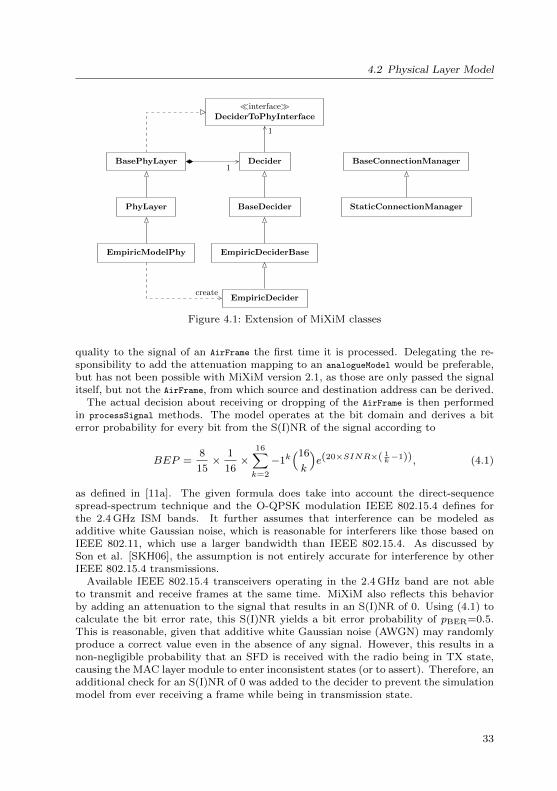
4.2 Physical Layer Model
1
1
create
BasePhyLayer
PhyLayer
EmpiricModelPhy
Decider
BaseDecider
EmpiricDeciderBase
EmpiricDecider
BaseConnectionManager
StaticConnectionManager
�interface�DeciderToPhyInterface
Figure 4.1: Extension of MiXiM classes
quality to the signal of an AirFrame the first time it is processed. Delegating the re-sponsibility to add the attenuation mapping to an analogueModel would be preferable,but has not been possible with MiXiM version 2.1, as those are only passed the signalitself, but not the AirFrame, from which source and destination address can be derived.
The actual decision about receiving or dropping of the AirFrame is then performedin processSignal methods. The model operates at the bit domain and derives a biterror probability for every bit from the S(I)NR of the signal according to
BEP =8
15×
1
16×
16∑k=2
−1k(16
k
)e(20×SINR×( 1
k−1)), (4.1)
as defined in [11a]. The given formula does take into account the direct-sequencespread-spectrum technique and the O-QPSK modulation IEEE 802.15.4 defines forthe 2.4 GHz ISM bands. It further assumes that interference can be modeled asadditive white Gaussian noise, which is reasonable for interferers like those based onIEEE 802.11, which use a larger bandwidth than IEEE 802.15.4. As discussed bySon et al. [SKH06], the assumption is not entirely accurate for interference by otherIEEE 802.15.4 transmissions.
Available IEEE 802.15.4 transceivers operating in the 2.4 GHz band are not ableto transmit and receive frames at the same time. MiXiM also reflects this behaviorby adding an attenuation to the signal that results in an S(I)NR of 0. Using (4.1) tocalculate the bit error rate, this S(I)NR yields a bit error probability of pBER=0.5.This is reasonable, given that additive white Gaussian noise (AWGN) may randomlyproduce a correct value even in the absence of any signal. However, this results in anon-negligible probability that an SFD is received with the radio being in TX state,causing the MAC layer module to enter inconsistent states (or to assert). Therefore, anadditional check for an S(I)NR of 0 was added to the decider to prevent the simulationmodel from ever receiving a frame while being in transmission state.
33
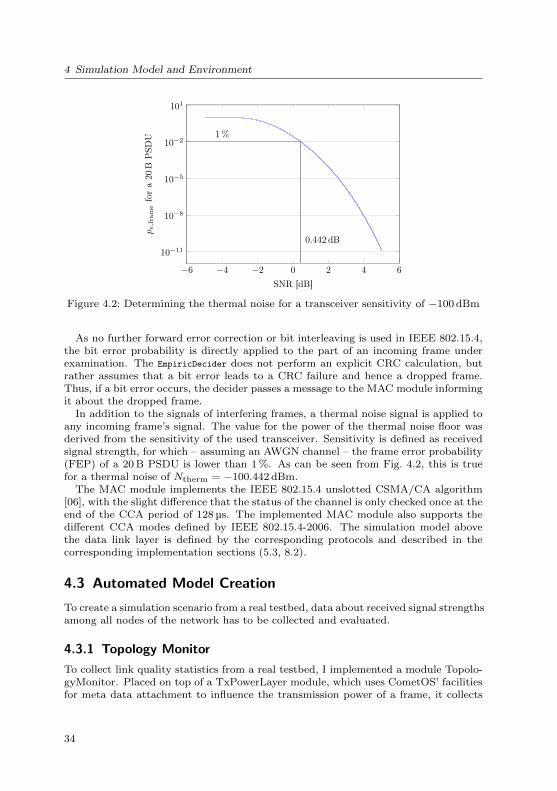
4 Simulation Model and Environment
−6 −4 −2 0 2 4 6
10−11
10−8
10−5
10−2
101
0.442 dB
1%
SNR [dB]
pe,fra
me
for
a20
BP
SDU
Figure 4.2: Determining the thermal noise for a transceiver sensitivity of −100 dBm
As no further forward error correction or bit interleaving is used in IEEE 802.15.4,the bit error probability is directly applied to the part of an incoming frame underexamination. The EmpiricDecider does not perform an explicit CRC calculation, butrather assumes that a bit error leads to a CRC failure and hence a dropped frame.Thus, if a bit error occurs, the decider passes a message to the MAC module informingit about the dropped frame.
In addition to the signals of interfering frames, a thermal noise signal is applied toany incoming frame’s signal. The value for the power of the thermal noise floor wasderived from the sensitivity of the used transceiver. Sensitivity is defined as receivedsignal strength, for which – assuming an AWGN channel – the frame error probability(FEP) of a 20 B PSDU is lower than 1 %. As can be seen from Fig. 4.2, this is truefor a thermal noise of Ntherm = −100.442 dBm.
The MAC module implements the IEEE 802.15.4 unslotted CSMA/CA algorithm[06], with the slight difference that the status of the channel is only checked once at theend of the CCA period of 128 µs. The implemented MAC module also supports thedifferent CCA modes defined by IEEE 802.15.4-2006. The simulation model abovethe data link layer is defined by the corresponding protocols and described in thecorresponding implementation sections (5.3, 8.2).
4.3 Automated Model Creation
To create a simulation scenario from a real testbed, data about received signal strengthsamong all nodes of the network has to be collected and evaluated.
4.3.1 Topology Monitor
To collect link quality statistics from a real testbed, I implemented a module Topolo-gyMonitor. Placed on top of a TxPowerLayer module, which uses CometOS’ facilitiesfor meta data attachment to influence the transmission power of a frame, it collects
34

4.3 Automated Model Creation
−3 −2 −1 0 1 2 3 4 5 610−12
10−8
10−4
100
SNR[dB]
pe,fra
me
20B PSDU96B PSDU
Figure 4.3: FEP (pe,frame) against SINR for different frame sizes
statistics about a node’s neighborhood. Two parameters govern its behavior: a periodand a frame size. When activated, the TopologyMonitor transmits a broadcast framewith the configured size at a random point in time during each period. The RSSI ofincoming frames as reported by the radio driver and its square value are accumulatedand stored for each source address, i.e., neighbor. Additionally, the overall count of re-ceived frames and the number of occurrences of the minimum RSSI value of −90 dBm(see Sect. 4.2.3) is stored. Each node also keeps track of the number of broadcastframes sent.
The frame size was chosen as 96 B to reflect the size of data frames during a6LoWPAN fragmentation experiment. Using frames of smaller size slightly under-estimates the potential for frame errors (Fig. 4.3). The interval of sending was setto Tinterval = 2 s to reach a reasonable trade-off between introducing a probabilityfor collisions, which are not desired, and the runtime necessary to get a significantnumber of samples. The probability for an interval without any collisions under theassumption of independent frame transmissions can be calculated as
Pnone =
[1− (n− 1)
Ttx
Tinterval
]n(4.2)
with Ttx being transmission duration for a frame and n the number of nodes withininterference range. The formula neglects that transmissions are actually not inde-pendent due to the CSMA/CA algorithm, that usually not all n nodes will be withininterference range of each other and that frames are not always transmitted completelywithin the interval. For a network of 13 nodes (like the Telematics testbed), for thegiven values a probability of
Pnone =
[1− (13− 1)
(96 + 10 + 2 + 4)× 8bit
2× 250 kbit
]13
≈ 0.75 (4.3)
can be estimated as worst case for the probability of no frame collisions within a singlebroadcast interval.
4.3.2 Post-Processing
The data containing RSSI and the number of frames is used to create a log-normaldistribution of incoming RSSI values and to determine a static routing topology.
35

4 Simulation Model and Environment
−106 −102 −98 −94 −90 −86 −820
1
2
·10−2
RSSI[dBm]
Est
imat
edP
DF
0
0.2
0.4
0.6
0.8
1
Rel
.fr
eque
ncy
inbi
ns
Figure 4.4: Derivation of normal distribution from data collected by the TopologyMon-itor; Resulting normal distribution (left y-axis) and relative frequency ofsamples in bins (right y-axis)
Estimate Normal Distribution
As described in Sect. 4.2.3, the transceiver used for the testbed experiments (AtmelATmega128RFA1) does report RSSI and ED values with a minimum value of Pmin =−90 dBm. However, average values of −90 dBm can be observed for links with anexpected transmission count (ETX, [De +03]) of near 1 as well as links with muchlarger ETX. Given the transceiver’s sensitivity of −100 dBm this does not come as asurprise.
To get a better estimate of each link in terms of a fixed average plus stochasticlog-normal component, the samples of the received signal strength are classified intothree bins and for each the number of frames ncase is determined (Fig. 4.4):
• “regular” bin (nregular): number of frames with RSSI > Pmin
• “minimum” bin (nmin): all logged minimum values (Sect. 4.3.1)) fall into thiscategory (Pmin ≥ RSSI > Ploss)
• “loss” bin (nloss): all frames that have not been received are considered to fallinto this category (RSSI < Ploss)
The boundary for lost frames is set to Ploss = −102 dBm. These three bins are thenused to calculate the parameters of a corresponding normal distribution. Given thecumulative distribution function of the normal distribution
F (x) =1
2
(1 + erf
(x− µ√
2σ2
)), (4.4)
and the number of samples in each bin known, a system of two equations can becreated:
(I) F (Pmin) =nmin + nloss
nall
(II) F (Ploss) =nloss
nall,
(4.5)
36
4.3 Automated Model Creation
which is equivalent to
(I) Xm = erf−1
(2nmin + nloss
nall− 1
)=
Pmin − µ√σ2
(II) Xl = erf−1
(2nloss
nall− 1
)=
Ploss − µ√σ2
,
(4.6)
with erf−1(x) being the inverse of the erf function. Solving the system for for µ andσ2 yields
µ =XmPloss −XlPmin
Xm −Xl(4.7)
σ2 = 0.5
(Pmin − Ploss
Xm −Xl
)2
(4.8)
Considering all three bins (the “regular” bin is implicitly included by adding to thetotal number of frames sent), this method yields a unique normal distribution.
A problem with this approach is caused by frames that are lost due to interference,e.g., collisions with other frames. Those may cause a distribution with a large numberof frames in the regular bin and a significantly smaller number of frames in the min-imum and loss bins, with nloss > nmin. To mitigate this problem, sample mean andunbiased sample variance are directly calculated from all regular samples, ignoringthe frames in the other bins, if the number of regular frames is much larger than thenumber of frames in the other bins. “Much larger” in this context means that theother bins contain less than 0.5 % of the frames in the regular bin. Additionally, in theother case, for each sample in the minimum and loss bins, a value is drawn from thederived normal distribution. These newly created values and the actually measuredvalues from the regular bin are then considered a complete sample. The sample meanand variance of this sample then define the final normal distribution.
The thus calculated distributions with µRSSI and variance define the physical layerof the simulation model and are used as link properties by the StaticConnectionManager
and the EmpiricDecider (see Sect. 4.2.3).
Static Routing Topology
The link properties as derived in Sect. 4.3.2 are – in combination with the recordedETX values – also used as input to determine the static routing topology of thesimulation model. They form a weighted directed graph representing the networkconnectivity. To tackle the problem of time-variant links that may cause a statictopology to become disconnected (as discussed in Sect. 4.2.3), some adjustments aremade to the weights. As basic weight, the measured ETX value is used. Penalties tothis basic weight are applied for links with an average RSSI below a certain thresholdand links with highly varying RSSI to derive the adjusted weight w:
w =
{ETX + kabs × (RSSIth − RSSI) + kσ2 × σ2
RSSI RSSI < RSSIthETX + kσ2 × σ2
RSSI else(4.9)
37

4 Simulation Model and Environment
Hence, links with a good and stable RSSI are preferred to those with a weak andhighly varying RSSI, depending on the constant penalty factors kabs and kσ2 . Theadjusted weight of the two edges between any two nodes u and v (one for each directionof communication) is then further combined to a bi-directional weight:
wbi = wuv × wvu (4.10)
The resulting weight yields the ETX for the unicast transmission of a frame underthe assumption that frame and acknowledgment have the same probability of success.While this assumption does not hold true due to the different frame sizes of ACK anddata frames, bi-directional (and not asymmetric) links are needed nonetheless. Therouting topology is found by applying the Dijkstra algorithm [Dij] to the undirectedgraph with the bi-directional weights.
4.4 Confidence Intervals
To make significant statements about the results collected from experiments and simu-lations, multiple runs of all experiment configurations were conducted and confidenceintervals calculated for the expectation values of measured quantities. Student’s t-distribution was used to calculate confidence intervals according to[
x− t(1−α2
;n−1)S√n, x+ t(1−α
2;n−1)
S√n
], (4.11)
with sample mean x, the sample variance S2 and the (one-sided) (1 − α2
)-percentileof the t-distribution with n − 1 degrees of freedom, t(1−α
2;n−1). Unless specified
differently, 95 % confidence intervals where calculated, resulting in α = 0.05.
38
5 Basic Forwarding Techniques for6LoWPAN-Fragmented Datagrams
This chapter introduces a first simulative and experimental evaluation of basic andenhanced route-over forwarding strategies for 6LoWPAN. The results are included inthis thesis because they illustrate the necessity of an accurate simulation model asdeveloped in Chapter 4.
5.1 Related Work
Ludovici et al. evaluated different 6LoWPAN forwarding techniques for IPv6 data-grams with and without fragmentation [LCC11]. They analyzed end-to-end delay andpacket reception rate (PRR) for a single sender for two route-over and two mesh-under schemes for a line topology of up to five TelosB nodes. They call the modesthey define in addition to plain route-over and mesh-under “enhanced route-over” and“controlled mesh-under”. The former uses basically the same approach as our Direct(2.2.3): fragments are forwarded immediately and upon reception of the first fragmenta virtual circuit is installed, which is used to route subsequent fragments along thesame path. The latter mode adds additional checks to the mesh-under forwardingprocess. If a node receives an out-of-order fragment, it solicits its predecessor for themissing fragment. If the missing fragment is not recovered, the node will stop forward-ing any fragments belonging to that datagram. In contrast, their plain mesh-underforwarding also forwards fragments of datagrams that have already been lost.
The results of Ludovici et al. show comparatively high end-to-end latency for theroute-over forwarding mode. This is attributed to the reassembly of the whole data-gram at every hop. The other three modes perform similar to each other, with plainmesh-under exhibiting slightly higher latency, especially for the shorter paths. Consid-ering the packet reception rates, high losses for larger fragments have been observed.For mesh-under, controlled mesh-under and enhanced route-over, the loss rates in-crease (non-linearly) from 0 for datagrams of 100 B to over 0.4 for datagrams of 1100 B,with plain mesh-under performing worst. The high loss rates were attributed to colli-sions on the wireless channel. Considering the short distance of only four hops, withonly a single node transmitting, the measured performance appears to be very bad.For the plain route-over mode, the performance in terms of loss rate is significantlybetter (below 0.04) for “small” datagrams, i.e., those with a payload of less than 900 B.For larger datagrams, buffer drops cause the drop rate to increase to 0.58 for data-grams of 1100 B, i.e., even worse than the mesh-under mode. In general, the resultsshow a need for further investigation of 6LoWPAN fragmentation performance.
Bhunia et al. carried out similar experiments and also analyzed end-to-end delaysand loss rates for a small testbed of three nodes. Like Ludovici et al. they usedTelosB motes running the TinyOS blip stack [DC12]. Their results are in accord with
39

5 Basic Forwarding Techniques for 6LoWPAN-Fragmented Datagrams
those of Ludovici et al. and also show very high loss rates when transmitting largedatagrams (> 900 B). A modified route-over scheme, which is claimed to implementa retransmission procedure for missed fragments is shown to slightly outperform theplain modes in the given scenario.
Toscano and Lo Bello evaluated the performance of ZigBee [12b] and 6LoWPAN forlow-power industrial scenarios [TB12]. They also used TelosB nodes running TinyOSwith the TKN154 [Hau09] to realize a beacon-enabled IEEE 802.15.4 cluster-tree andthe blip stack for the 6LoWPAN network, applying low-power listening. Care wastaken to tune the duty-cycles of the two different schemes to comparable values andan analysis of how to choose the correct settings for beacon and superframe order forbeacon-enabled mode and the active and sleeping periods for 6LoWPAN networks ispresented. For low data rate applications they evaluated latency, packet reception rateand update time (the time between packet receptions). From the observed results, anumber of conclusions are drawn:
• 6LoWPAN duty cycle depends on the overall network load, making it difficultto plan energy consumption beforehand.
• The IEEE 802.15.4/ZigBee network is able to support lower duty cycles withacceptable performance.
• For higher duty cycles, 6LoWPAN exhibits smaller end-to-end delays and higherreliability.
Wang et al. [Zhu+13] proposed a technique for mesh-under routing in 6LoWPANs,which reassembles packets at some intermediate nodes. Evaluating route-over, mesh-under and their chained mesh-under routing (C-MUR) in a testbed consisting of sixnodes arranged in a line topology, they observed that C-MUR achieves a latencybetween mesh-under and route-over and a better packet reception rate than both foran increasing number of fragments.
A typical issue encountered in multi-hop mesh networks is self-interference, as de-scribed in Sect. 2.2.3. This was recognized in the research community of wireless sensornetworks. In their publication on the collection tree protocol (CTP), which heavilyinspired RPL, Gnawali et al. proposed to decrease the maximum rate at which nodesforward frames via CTP [Gna+09]. They determined the optimal delay experimen-tally in a small testbed. Optimal in that sense means achieving the best trade-offbetween reliability and throughput. Based on this investigation, they set the intervala node waits after each transmission to 1.5 to 2.5 times the expected transmissiontime.
The Flush protocol for bulk data transfer [Kim+07a] also recognizes the need todelay consecutive transmissions along the same path. It installs two mechanisms toprevent self-interference. First, information about transmission time estimates of anode and its successor are piggybacked to every data frame. This information issnooped by preceding nodes on the path and used to adapt their own transmissionrate. Secondly, nodes refrain from transmitting with higher rates than any other nodealong the path. This information is propagated from the destination (root of a routingtree) back to the origin of the transmission.
40
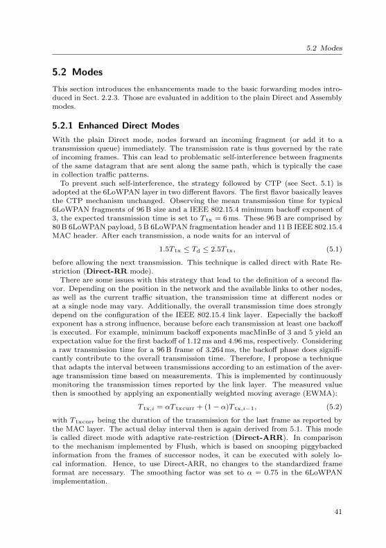
5.2 Modes
5.2 Modes
This section introduces the enhancements made to the basic forwarding modes intro-duced in Sect. 2.2.3. Those are evaluated in addition to the plain Direct and Assemblymodes.
5.2.1 Enhanced Direct Modes
With the plain Direct mode, nodes forward an incoming fragment (or add it to atransmission queue) immediately. The transmission rate is thus governed by the rateof incoming frames. This can lead to problematic self-interference between fragmentsof the same datagram that are sent along the same path, which is typically the casein collection traffic patterns.
To prevent such self-interference, the strategy followed by CTP (see Sect. 5.1) isadopted at the 6LoWPAN layer in two different flavors. The first flavor basically leavesthe CTP mechanism unchanged. Observing the mean transmission time for typical6LoWPAN fragments of 96 B size and a IEEE 802.15.4 minimum backoff exponent of3, the expected transmission time is set to T tx = 6 ms. These 96 B are comprised by80 B 6LoWPAN payload, 5 B 6LoWPAN fragmentation header and 11 B IEEE 802.15.4MAC header. After each transmission, a node waits for an interval of
1.5T tx ≤ Td ≤ 2.5T tx, (5.1)
before allowing the next transmission. This technique is called direct with Rate Re-striction (Direct-RR mode).
There are some issues with this strategy that lead to the definition of a second fla-vor. Depending on the position in the network and the available links to other nodes,as well as the current traffic situation, the transmission time at different nodes orat a single node may vary. Additionally, the overall transmission time does stronglydepend on the configuration of the IEEE 802.15.4 link layer. Especially the backoffexponent has a strong influence, because before each transmission at least one backoffis executed. For example, minimum backoff exponents macMinBe of 3 and 5 yield anexpectation value for the first backoff of 1.12 ms and 4.96 ms, respectively. Consideringa raw transmission time for a 96 B frame of 3.264 ms, the backoff phase does signifi-cantly contribute to the overall transmission time. Therefore, I propose a techniquethat adapts the interval between transmissions according to an estimation of the aver-age transmission time based on measurements. This is implemented by continuouslymonitoring the transmission times reported by the link layer. The measured valuethen is smoothed by applying an exponentially weighted moving average (EWMA):
T tx,i = αT txcurr + (1− α)T tx,i−1, (5.2)
with T txcurr being the duration of the transmission for the last frame as reported bythe MAC layer. The actual delay interval then is again derived from 5.1. This modeis called direct mode with adaptive rate-restriction (Direct-ARR). In comparisonto the mechanism implemented by Flush, which is based on snooping piggybackedinformation from the frames of successor nodes, it can be executed with solely lo-cal information. Hence, to use Direct-ARR, no changes to the standardized frameformat are necessary. The smoothing factor was set to α = 0.75 in the 6LoWPANimplementation.
41

5 Basic Forwarding Techniques for 6LoWPAN-Fragmented Datagrams
IPForward
UDPICMP
Lowpan LowpanQueue
�interface�QueueObject
QueueFrame QueuePacketMAL
�interface�FragmentHandler
DirectHandler
AssemblyHandler
StaticRoutingTable
NeighborDiscovery
StaticRouting
Figure 5.1: High level UML class diagram of 6LoWPAN implementation; double linesrepresent CometOS message exchange
5.2.2 Retry Control
This chapter also includes an approach from a different angle. With 6LoWPAN frag-mentation, the loss of a single fragment results in the loss of the whole datagram,unless some recovery mechanism is applied. Fragments that have been transmittedup to that point have been transmitted in vain and produced network traffic thatdoes not add to the goodput of the network. In lossy wireless networks, link layerretransmissions are desperately needed to prevent high loss rates, which can also beconcluded from the results of the analytical model presented in Sect. 3.3. This istaken into account by setting the number of link layer retries to the IEEE 802.15.4maximum value of 7 (cf. Sect. 5.4). To further prevent the loss of nearly completelytransmitted datagrams, the idea of PRC is to increase the number of maximum frameretransmissions the more fragments have been transmitted already. With sdg beingthe size of the fragmented datagram and sdg,trans the accumulated size of fragmentsalready transmitted of that datagram, the number of retries rPRC is calculated by
rPRC = 7 + 8×sdg,trans
sdg. (5.3)
This results in a number of 7 to 15 MAC retransmissions, with 15 being the maximumnumber provided by the transceiver’s hardware-supported automatic acknowledgmentmode (see Sect. 6.1) used for the testbed experiments described in this chapter.
5.3 6LoWPAN Implementation
Figure 5.1 shows the high-level structure of the 6LoWPAN module for CometOS. Forsimplification, the result of an additional refactoring for the implementation of LFFR
42

5.3 6LoWPAN Implementation
(cf. Sect. 2.2.5) is not depicted here. The main component is the Lowpan module, whichinteracts via CometOS message passing with the IEEE 802.15.4-like link layer moduleat one and the IPv6 module at the other side. If Lowpan detects a fragmentation header,it passes the incoming fragment to a FragmentHandler.
The FragmentHandler interface represents the actual and virtual reassembly buffersused for the Assembly and Direct modes of operation (Fig. 5.1). Note that the formeris needed in both modes of operation for reassembling datagrams that are destined toa node.
The AssemblyHandler delegates the reassembling process to a DatagramReassembly ob-ject, which manages identification (tag, size, source address), decompression, transitstatus (bit vector of arrived 8 octet units), timeout information and data storage.
The maximum duration of the (virtual) reassembly process is bounded by a timeout,which is implemented by an aging algorithm. A single timer is initialized to fireevery Ito. Given a timeout period Tto, the creation of a reassembly or virtual buffer
forwarding process is initialized with a counter Nto =⌈TtoIto
⌉+ 1 and is decremented
by one every Ito. The counter always reaches zero after a duration in the interval[Tto, Tto + Ito], in which case the timeout is fired and the process aborted. Becauseonly a single timer is needed to implement this strategy (in contrast to one timerfor every reassembly process) memory and CPU resources can traded for accuracy ofthe timeout. Our 6LoWPAN implementation uses a most trivial configuration withIto = Tto.
IPHC decompression and compression are implemented according to RFC6282 [HT11]and are not described in detail in this thesis.
In a similar way, DirectHandler uses PacketInformation objects that manages the stateof an IPv6 datagram in transit. Different from DatagramReassembly, it has to addition-ally store the outgoing tag of the datagram, which is fixed after the DirectHandler
asked the IPv6 module for a routing decision.Both fragment handlers use a global 6LoWPAN buffer to store datagrams and
fragments. The AssemblyHandler always tries to reserve space in the buffer for thewhole incoming datagram upon reception of the first fragment. As soon as fragmentsare transmitted successfully, the buffer space is partially released.
The actual forwarding of fragments is managed by a generic queue, which acceptsobjects that implement the QueueObject interface. This interface contains methodsto generate frames, process replies from the link layer and and retrieve some statusinformation. There are two basic types of object representing the different concepts.
• A QueuePacket represents a complete datagram. Objects of this type are addedto the queue for datagrams originating at a node in both modes of operationand for forwarded datagrams in Assembly mode, i.e., every time a data requestis received from the IPv6 module.
• A QueueFrame represents a single fragment and is enqueued every time a 6LoWPANfragment is received from the MAC layer in Direct mode.
The Lowpan module queries the queue for the next object every time it is ready to send,i.e., a transmission has finished and the rate restriction mechanism (if used) allowsthe next transmission. As soon as a link-layer response is received, the result is passedto the corresponding QueueObject, which is responsible for updating the transmission
43

5 Basic Forwarding Techniques for 6LoWPAN-Fragmented Datagrams
MacDisp
TxPwrAODV TssDisp
NwkDisp 6loDisp Tss
SRL OTAP Lowpan Topo
RA IP Routing
UDP TrafficICMP
0 1 2
10 6lo 0
0
NIS
MACSC
MacDisp
AODV TssDisp
NwkDisp 6loDisp Tss
SRL PyOTAP Lowpan Topo
PyRA IP Routing
UDP PyTrafficICMP
01
2
10 6lo 0
0
SC
Basestation Gateway node
Figure 5.2: CometOS stack used at the at the basestation and the node attached to thebasestation, with control stack (blue) and 6LoWPAN stack (green). ’Py’-prefixed modules are specialized basestation modules. Dashed lines repre-sent message-passing connections via CometOS gates. Numbers representprotocol identifiers added to/removed from a frame by the dispatcher mod-ule.
status. This comprises checking for completion of the transfer or – in case of failure– to delete all traces of the datagram in the buffer. This implementation implies thatdatagrams encapsulated in a QueuePacket are handled continuously until completion.QueueFrame-encapsulated fragments of datagrams in transit may interleave with eachother or with a complete QueuePacket-encapsulated datagram originating at the node.
5.4 Experiment Setup
This section describes the simulated network topologies and the configuration of thetestbed experiments. Furthermore, the mechanism used for time synchronization inthe testbed is introduced. The presented evaluation is subdivided into two sets ofsimulations and experiments, simply named first and second set of experiments. Dif-ferences between those two sets are described in the corresponding subsection.
5.4.1 Testbed
For the purpose of validation, we used a testbed consisting of 13 dresden electronicdeRFmega128-22A00 modules equipped with an Atmel ATmega128RFA1 controllerwith integrated IEEE 802.15.4 transceiver operating in the 2.4 GHz ISM band. Itprovides 128 KiB of program memory and 16 KiB of RAM, which was enough to run
44
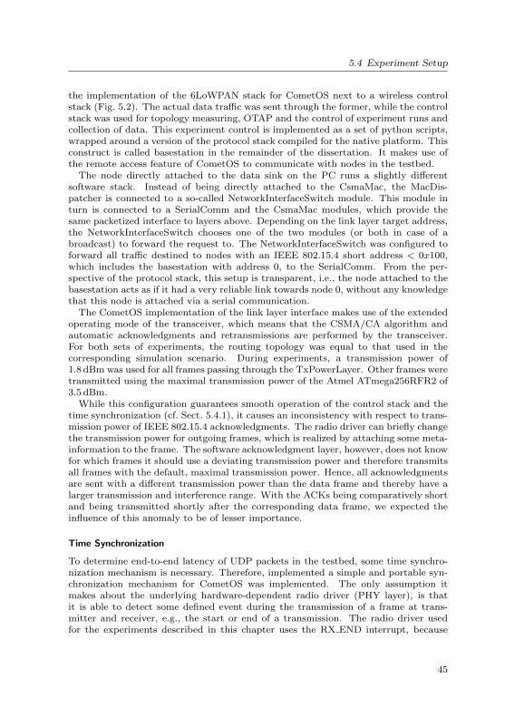
5.4 Experiment Setup
the implementation of the 6LoWPAN stack for CometOS next to a wireless controlstack (Fig. 5.2). The actual data traffic was sent through the former, while the controlstack was used for topology measuring, OTAP and the control of experiment runs andcollection of data. This experiment control is implemented as a set of python scripts,wrapped around a version of the protocol stack compiled for the native platform. Thisconstruct is called basestation in the remainder of the dissertation. It makes use ofthe remote access feature of CometOS to communicate with nodes in the testbed.
The node directly attached to the data sink on the PC runs a slightly differentsoftware stack. Instead of being directly attached to the CsmaMac, the MacDis-patcher is connected to a so-called NetworkInterfaceSwitch module. This module inturn is connected to a SerialComm and the CsmaMac modules, which provide thesame packetized interface to layers above. Depending on the link layer target address,the NetworkInterfaceSwitch chooses one of the two modules (or both in case of abroadcast) to forward the request to. The NetworkInterfaceSwitch was configured toforward all traffic destined to nodes with an IEEE 802.15.4 short address < 0x100,which includes the basestation with address 0, to the SerialComm. From the per-spective of the protocol stack, this setup is transparent, i.e., the node attached to thebasestation acts as if it had a very reliable link towards node 0, without any knowledgethat this node is attached via a serial communication.
The CometOS implementation of the link layer interface makes use of the extendedoperating mode of the transceiver, which means that the CSMA/CA algorithm andautomatic acknowledgments and retransmissions are performed by the transceiver.For both sets of experiments, the routing topology was equal to that used in thecorresponding simulation scenario. During experiments, a transmission power of1.8 dBm was used for all frames passing through the TxPowerLayer. Other frames weretransmitted using the maximal transmission power of the Atmel ATmega256RFR2 of3.5 dBm.
While this configuration guarantees smooth operation of the control stack and thetime synchronization (cf. Sect. 5.4.1), it causes an inconsistency with respect to trans-mission power of IEEE 802.15.4 acknowledgments. The radio driver can briefly changethe transmission power for outgoing frames, which is realized by attaching some meta-information to the frame. The software acknowledgment layer, however, does not knowfor which frames it should use a deviating transmission power and therefore transmitsall frames with the default, maximal transmission power. Hence, all acknowledgmentsare sent with a different transmission power than the data frame and thereby have alarger transmission and interference range. With the ACKs being comparatively shortand being transmitted shortly after the corresponding data frame, we expected theinfluence of this anomaly to be of lesser importance.
Time Synchronization
To determine end-to-end latency of UDP packets in the testbed, some time synchro-nization mechanism is necessary. Therefore, implemented a simple and portable syn-chronization mechanism for CometOS was implemented. The only assumption itmakes about the underlying hardware-dependent radio driver (PHY layer), is thatit is able to detect some defined event during the transmission of a frame at trans-mitter and receiver, e.g., the start or end of a transmission. The radio driver usedfor the experiments described in this chapter uses the RX END interrupt, because
45

5 Basic Forwarding Techniques for 6LoWPAN-Fragmented Datagrams
accuracy iMin iMax k noReset
5 ms 50 ms 12 5 false
Table 5.1: Parameters for CometOS simple time synchronization mechanism
a TX START interrupt is not available with at the Atmel ATmega128RFA11. Thispoint in time is then considered to refer to the same point in real time at both nodes,neglecting the propagation delay of the frame. For the purpose of determining thelatency of large datagrams, which is in the order of several tens of milliseconds, apropagation delay of about 1 µs (for 300 m) is considered negligible.
The synchronization mechanism uses a two kinds of broadcasts to propagate a jointnetwork time from a master node to all nodes in the network. Every time updateconsists of two messages:
• The InitialMessage contains only a depth field containing the distance of thesender (in hops) to the master of the time synchronization process. A receiverstores a local timestamp corresponding to a defined event of the reception.
• The TimestampMessage contains the network timestamp of the defined event. Thistimestamp is used by the receiver for synchronization.
Only nodes that consider themselves as synchronized transmit time updates. Hence,time updates originate at the master first and propagate into the network from there.Nodes only process time updates that originate from “parents”, i.e., nodes nearer tothe sink.
The transmission of time updates is governed by the Trickle algorithm [Lev+11].Nodes only transmit a timer update if they haven’t received k consistent transmissionsof other nodes. Consistent in that context means that a time update from a parentdoes not deviate from the current network time of a node by a configurable accuracyparameter. If, on the other hand, an inconsistent time update is received, the timesynchronization mechanism optionally resets Trickle to enable fast propagation ofthis time update through the network. Because such a reset of Trickle temporarilyincreases the traffic significantly, an option to prevent resetting was added. Thereby,after a starting phase, time updates are sent using a fixed interval range, reducing theburstiness of the time synchronization traffic at the cost of allowing some inaccuraciesin time synchronization.
For the testbed, Trickle was configured according to Tbl. 5.1, yielding a intervalrange for time updates of [51.2 s, 102.4 s] in a stable state. The used board (dresdenelectronic deRFmega128-22A00, [11b]) connects the Atmel ATmega128RFA1 clockinput to a crystal oscillator with a maximum deviation of ±10 ppm and therefore theclock drift between any two nodes in the network should stay below 0.2 ms for anupdate period. To verify that the time synchronization mechanism did only send anegligible number of frames, the number of transmissions and resets was logged andrecorded for each node at the end of each experiment. Thereby, it could be verifiedthat the interval of time updates corresponded to the maximum Trickle interval.
1This restriction and the fact that the extended mode of operation is used is the reason for makingthe time synchronization flexible
46

5.4 Experiment Setup
Memory usage
For our first set of experiments, the 6LoWPAN layer of our implementation had a6LoWPAN data buffer of 2000 B. This buffer is used for reassembly, buffering en-queued fragments and as a data storage for datagrams to be transmitted. For thesecond set of experiments we reduced the buffer size to the IPv6 minimum MTU of1280 B.
In the Assembly Mode, we set assembly_entries to 10, i.e., up to 10 datagrams canbe reassembled at the same time (given that their combined size fits into the buffer).Because the Direct modes only reassemble datagrams which are destined to the nodeitself, we reduce this value to 4 for those. The direct modes use a virtual fragmentbuffer, which keeps track of the state of up to 15 in-transit datagrams. With thisconfiguration, both modes use about the same amount of RAM yielding a basis for afair comparison. Concerning program memory, our implementation of the Direct modeuses 3910 B more than the corresponding implementation of the Assembly mode. Asthe Direct mode basically has to provide the same assembly service for packets destinedto the node itself, plus offering the additional services for direct forwarding, this is tobe expected. The rate-restricted modes mainly use a single variable of 2 B to storethe current estimated transmission time and a CometOS timer object which is startedafter each transmission corresponding to 5.1.
While the nodes are constrained with regard to the size of the 6LoWPAN data bufferand data structures storing information reassembly or forwarding, for all experimentswe provided the base station with buffers and structures large enough to not causeany drops of datagrams. We deem this approach reasonable as we expect 6LoWPANborder routers to be slightly more powerful devices, equipped with larger memories.
5.4.2 Simulation
The configuration of the simulation adopts the methodology presented in Chapter 4,with some exceptions. For our first set of experiments, we used a formula successfullyapplied in the iEZMesh project (Sect. 2.2.1), which used a sub-GHz transceiver andbinary frequency shift keying (BFSK) and consequently calculated the pe,BFSK by
pe,BFSK = 0.5× erfc
(√SINR
2
). (5.4)
This does not accurately represent the direct sequence spread-spectrum (DSSS)technique used at the IEEE 802.15.4 link layer and therefore shows a quite differ-ent curve compared to the one obtained by applying 4.1. The mismatch is shownin Fig. 5.3. Using the formula for BFSK, the FEP, denoted by pe,frame, starts todecrease at much larger values for signal to noise ratio (SNR) and the slope of thedecrease is less steep. This was accounted for by setting the thermal noise to a lowervalue of N0 = −105 dBm to get reasonable error probabilities for typical RSSI valuesbetween −85 dBm and −95 dBm. While this mitigates the inaccuracy of the modelfor transmissions in case only the thermal noise has to be considered, in case of in-terference the model still behaves differently from one using (4.1) to model DSSS.With (5.4), interference between frames most certainly causes frame drops unless onesignal is significantly stronger than the other one, i.e., SINR > 12 dB. This is different
47

5 Basic Forwarding Techniques for 6LoWPAN-Fragmented Datagrams
−6 −4 −2 0 2 4 6 8 10 12 14 16 1810−12
10−9
10−6
10−3
100
SNR[dB]
pe,fra
me
DSSSBFSK
Figure 5.3: FEP (pe,frame) to SNR for BFSK modulation and IEEE 802.15.4-DSSSwith O-QPSK for a PSDU of 96 B. For BFSK the FEP curve is shiftedand decreasing with a slope less steep.
from the DSSS model, for which interference between frames of slightly different signalstrength do not necessarily lead to a loss of both frames. The decision to stick with5.4 to calculate the FEP proved to introduce an unfavorable bias to the simulationresults, which will be discussed in Sect. 5.5.3.
The second set of experiments uses the more accurate formula to calculate the BEPthat is provided by the IEEE 802.15.4 standard and a thermal noise as defined inSect. 4.2.3.
The protocol stack used for the simulations above the MacAbstractionLayer is re-stricted to the 6LoWPAN stack (cf. Fig. 5.2). The control stack, TxPowerLayer andtime synchronization modules are not employed in a simulation environment.
5.4.3 Network Topologies
The evaluation in the first set of experiments concentrated on four different topologies(Fig. 5.4). The first three topologies are idealized, artificial constructs. The “Chain”network (Fig. 5.4a) was chosen as a network with potential for pipelining. In starkcontrast, the “Star” network has a maximum diameter of three and therefore does nothave any pipelining potential, but employs a bottle neck with regard to contentionfor the wireless channel and buffer space at its central node (Fig. 5.4b). Finally, theLong-Y network can be seen as a mixture of the two. In those three idealized networks,links are nearly perfect in the absence of interference, i.e., the FEP is near zero. Notethat for these networks, the routing tree and the actual wireless connections betweenthe nodes form the same graph. This means that in the Long-Y network, node 100and 200 are hidden-terminal from each others perspective when transmitting towardsnode 7.
The two “RealSim” networks were created from data collected in a real testbedwith the method described in Sect. 4.2.3. RS-A was evaluated in the first set of
48
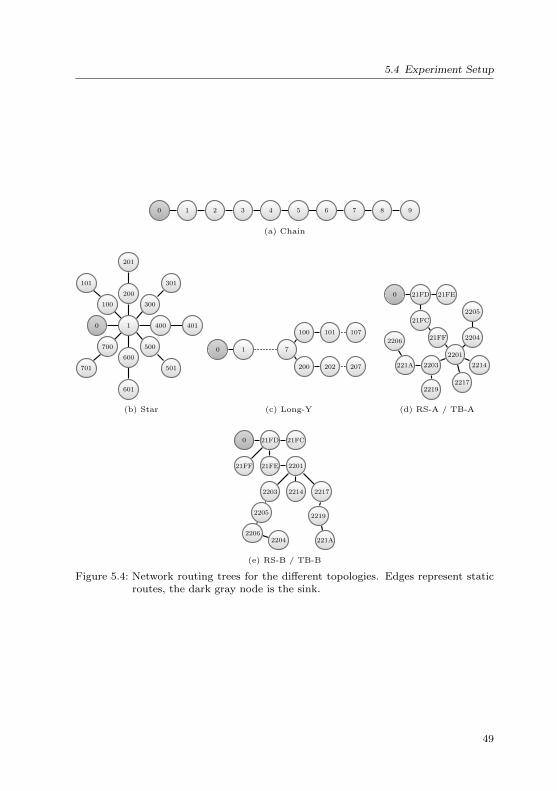
5.4 Experiment Setup
0 1 2 3 4 5 6 7 8 9
(a) Chain
0 1
100
200
300
400
500
600
700
101
201
301
401
501
601
701
(b) Star
0 1 7
100
200
101
202
107
207
(c) Long-Y
0 21FD 21FE
21FC
21FF
2201
2204
2205
2214
2217
2203
2219
2206
221A
(d) RS-A / TB-A
0 21FD 21FC
21FE21FF 2201
2203
2205
22062204
2214 2217
2219
221A
(e) RS-B / TB-B
Figure 5.4: Network routing trees for the different topologies. Edges represent staticroutes, the dark gray node is the sink.
49

5 Basic Forwarding Techniques for 6LoWPAN-Fragmented Datagrams
macMinBe (1st|2nd) macMaxBe macMaxCSMABackoffs macMaxFrameRetries
3|5 8 5 7
Table 5.2: Configuration of IEEE 802.15.4 link layer; macMinBe was varied between1st and 2nd set of experiments
experiments, RS-B in the second. Although the real nodes were deployed in the samerooms along a corridor in an office building at Hamburg University of Technology,the time between the first and second set of experiments was several months and thenodes had to be repositioned slightly. Therefore we decided to recreate the (routing)topology for the simulation. The resulting topologies are still similar with regard toaverage path length (3.62 for the first, 3.92 for the second set of experiments).
Instead of trying to simulate the serial connection in the testbed between basestationand the attached node (see Sect. 5.4.1), in the simulation environment we used awireless link with a constant strong signal of −50 dBm.
During some preliminary experiments, some links showed a strongly time-variantbehavior, i.e., the network became disconnected. To counter that effect, we measuredthe topology twice, once to determine a routing topology (for testbed and simulation)with lower transmission power of −6.5 dBm and once to collect link statistics for thesimulation with a higher one of 1.8 dBm. Thereby, routes are chosen more pessimisti-cally and more distant nodes are more likely to be within transmission range (but alsointerference range).
5.4.4 Traffic
We evaluated the performance of a collection traffic pattern for all networks. All nodesin the network periodically sent UDP packets of different sizes to the sink. To preventnodes from transmitting all at the same time, the interval i between two consecutiveUDP packet transmissions was randomized:
i = I +1
2λ, (5.5)
with I being uniformly distributed in[0, 1λ
]and λ = λB
LUDP, where λB and LUDP
denote the transmission rate of payload and the size of the individual UDP packet,respectively. This ensures a maximum interval between transmissions of UDP packetsfrom an arbitrary node in the network of imax = 3
2λ. This traffic pattern simulates a
collection of periodic data from all nodes in the wireless network.All nodes transmitted a constant total payload of 240 000 B and 48 000 B towards
the data sink in simulation and testbed, respectively. Hence, the total number of UDPpackets increased and the interval between the transmission of UDP packet decreasedwith increasing payload size, while the average transmission rate in terms of payloaddata was constant.
5.4.5 Link Layer Configuration
Because short tests with another macMinBe showed significantly different results forthe RS network in simulation, we conducted a second set of experiments for the slightly
50
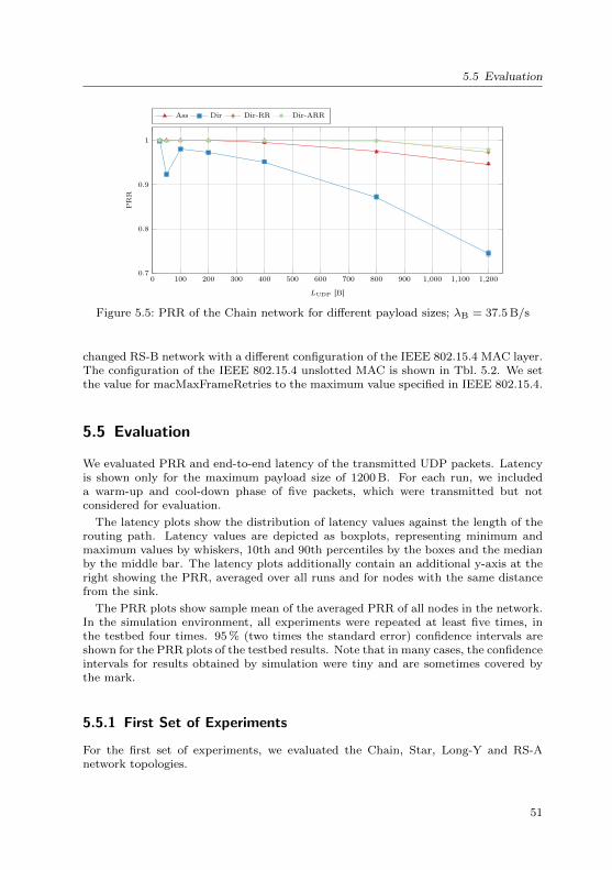
5.5 Evaluation
0 100 200 300 400 500 600 700 800 900 1,000 1,100 1,2000.7
0.8
0.9
1
LUDP [B]
PR
R
Ass Dir Dir-RR Dir-ARR
Figure 5.5: PRR of the Chain network for different payload sizes; λB = 37.5 B/s
changed RS-B network with a different configuration of the IEEE 802.15.4 MAC layer.The configuration of the IEEE 802.15.4 unslotted MAC is shown in Tbl. 5.2. We setthe value for macMaxFrameRetries to the maximum value specified in IEEE 802.15.4.
5.5 Evaluation
We evaluated PRR and end-to-end latency of the transmitted UDP packets. Latencyis shown only for the maximum payload size of 1200 B. For each run, we includeda warm-up and cool-down phase of five packets, which were transmitted but notconsidered for evaluation.
The latency plots show the distribution of latency values against the length of therouting path. Latency values are depicted as boxplots, representing minimum andmaximum values by whiskers, 10th and 90th percentiles by the boxes and the medianby the middle bar. The latency plots additionally contain an additional y-axis at theright showing the PRR, averaged over all runs and for nodes with the same distancefrom the sink.
The PRR plots show sample mean of the averaged PRR of all nodes in the network.In the simulation environment, all experiments were repeated at least five times, inthe testbed four times. 95 % (two times the standard error) confidence intervals areshown for the PRR plots of the testbed results. Note that in many cases, the confidenceintervals for results obtained by simulation were tiny and are sometimes covered bythe mark.
5.5.1 First Set of Experiments
For the first set of experiments, we evaluated the Chain, Star, Long-Y and RS-Anetwork topologies.
51

5 Basic Forwarding Techniques for 6LoWPAN-Fragmented Datagrams
0
0.2
0.4
0.6
0.8
1
PR
R
1 2 3 4 5 6 7 8 9
500
1,000
1,500
Hop
Late
ncy
[ms]
(a) Assembly Mode
0
0.2
0.4
0.6
0.8
1
PR
R
1 2 3 4 5 6 7 8 9
500
1,000
1,500
Hop
Late
ncy
[ms]
(b) Direct Mode
0
0.2
0.4
0.6
0.8
1
PR
R
1 2 3 4 5 6 7 8 9
500
1,000
1,500
Hop
Late
ncy
[ms]
(c) Direct-RR Mode
0
0.2
0.4
0.6
0.8
1
PR
R
1 2 3 4 5 6 7 8 9
500
1,000
1,500
Hop
Late
ncy
[ms]
(d) Direct-ARR Mode
Figure 5.6: Per hop latency and PRR in the Chain network with λB = 37.5 B/s and1200 B UDP payload; first set of experiments
Chain Network
In the Chain, the rate-restricted modes achieved better PRR – near 1 for packet sizesof up to 800 B – compared to the Assembly mode (Fig. 5.5), while the plain Directmode heavily suffers from packet losses caused by frame collisions. Main drop reasonin Assembly mode is lack of buffer space for reassembly, which is an issue especially forpayload sizes ≥ 400 B. The steep drop of the PRR at 50 B payload for the Direct modeis caused by a lack of IPv6 request objects at the 6LoWPAN layer. Those messagesare used by the DirectHandler to store addresses of fragmented datagrams in transit.Note that a UDP packet of 50 B payload has to be fragmented with our configurationand hence requires setting up transit state, which is not the case for 25 B packets.100 B packets, on the other hand, are transmitted with a smaller frequency, reducingthe required number of IPv6 request objects.
As expected, the direct modes exhibited lower median latency values, especially fornodes more distant to the sink (Fig. 5.6). With the plain Direct mode, the effect isless pronounced and the variation of the latency is considerably larger than for theAssembly mode and the rate-restricted modes. Considering the decrease of the PRRwith increasing distance of a node to the sink, the larger and more varying latencyin Direct mode can be explained with a comparatively large number of fragment re-
52
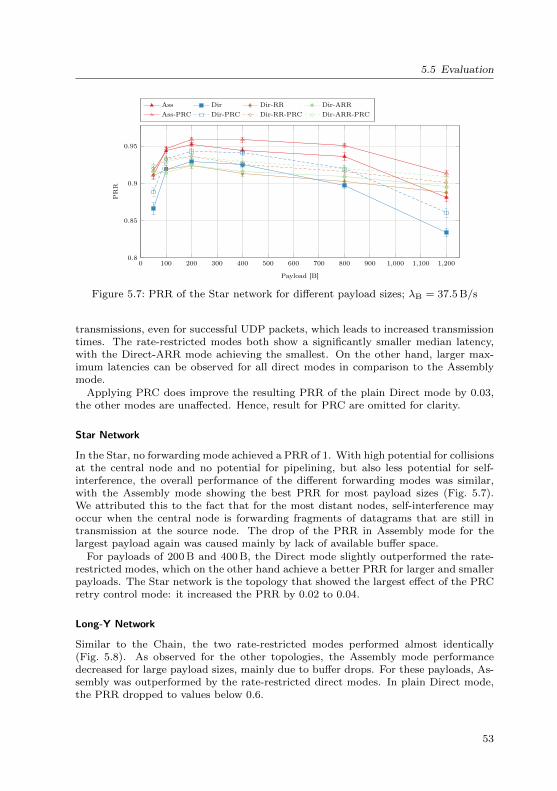
5.5 Evaluation
0 100 200 300 400 500 600 700 800 900 1,000 1,100 1,2000.8
0.85
0.9
0.95
Payload [B]
PR
RAss Dir Dir-RR Dir-ARRAss-PRC Dir-PRC Dir-RR-PRC Dir-ARR-PRC
Figure 5.7: PRR of the Star network for different payload sizes; λB = 37.5 B/s
transmissions, even for successful UDP packets, which leads to increased transmissiontimes. The rate-restricted modes both show a significantly smaller median latency,with the Direct-ARR mode achieving the smallest. On the other hand, larger max-imum latencies can be observed for all direct modes in comparison to the Assemblymode.
Applying PRC does improve the resulting PRR of the plain Direct mode by 0.03,the other modes are unaffected. Hence, result for PRC are omitted for clarity.
Star Network
In the Star, no forwarding mode achieved a PRR of 1. With high potential for collisionsat the central node and no potential for pipelining, but also less potential for self-interference, the overall performance of the different forwarding modes was similar,with the Assembly mode showing the best PRR for most payload sizes (Fig. 5.7).We attributed this to the fact that for the most distant nodes, self-interference mayoccur when the central node is forwarding fragments of datagrams that are still intransmission at the source node. The drop of the PRR in Assembly mode for thelargest payload again was caused mainly by lack of available buffer space.
For payloads of 200 B and 400 B, the Direct mode slightly outperformed the rate-restricted modes, which on the other hand achieve a better PRR for larger and smallerpayloads. The Star network is the topology that showed the largest effect of the PRCretry control mode: it increased the PRR by 0.02 to 0.04.
Long-Y Network
Similar to the Chain, the two rate-restricted modes performed almost identically(Fig. 5.8). As observed for the other topologies, the Assembly mode performancedecreased for large payload sizes, mainly due to buffer drops. For these payloads, As-sembly was outperformed by the rate-restricted direct modes. In plain Direct mode,the PRR dropped to values below 0.6.
53

5 Basic Forwarding Techniques for 6LoWPAN-Fragmented Datagrams
0 100 200 300 400 500 600 700 800 900 1,000 1,100 1,200
0.4
0.6
0.8
1
Payload [B]
PR
R
Ass Dir Dir-RR Dir-ARR
Figure 5.8: PRR of the Long-Y network for different payload sizes; λB = 37.5 B/s
0
0.2
0.4
0.6
0.8
1
PR
R
1 2 3 4 5 6 7 8 9 10 11 12 13 14 15
500
1,000
1,500
2,000
Hop
Late
ncy
[ms]
(a) Assembly Mode
0
0.2
0.4
0.6
0.8
1
PR
R1 2 3 4 5 6 7 8 9 10 11 12 13 14 15
500
1,000
1,500
2,000
Hop
Late
ncy
[ms]
(b) Direct Mode
0
0.2
0.4
0.6
0.8
1
PR
R
1 2 3 4 5 6 7 8 9 10 11 12 13 14 15
500
1,000
1,500
2,000
Hop
Late
ncy
[ms]
(c) Direct-RR Mode
0
0.2
0.4
0.6
0.8
1
PR
R
1 2 3 4 5 6 7 8 9 10 11 12 13 14 15
500
1,000
1,500
2,000
Hop
Late
ncy
[ms]
(d) Direct-ARR Mode
Figure 5.9: Per hop latency and PRR in the Long-Y network with λB = 37.5 B/s and1200 B payload; first set of experiments
54

5.5 Evaluation
0 200 400 600 800 1,000 1,2000.2
0.4
0.6
0.8
1
Payload [B]
PR
RAss Dir Dir-RR Dir-ARR
0 200 400 600 800 1,000 1,2000.2
0.4
0.6
0.8
1
Payload [B]
Figure 5.10: Comparing the packet reception rates of the RS-A and the TB-A networkswith a byterate of 37.5 B/s; first set of experiments
With the high potential for pipelining of fragments, the rate-restricted modes (Direct-RR: 395 ms, Direct-ARR: 392 ms) achieved median latencies of less than one third ofthat of the Assembly mode (1311 ms) for the largest payload size (Fig. 5.9). Again thiscame at the cost of a higher distance between 10th and 90th percentile and larger max-imum latencies. Different from the Chain network, the rate-restricted direct modesshowed a drop of the PRR beyond the bottleneck node (node 7 in Fig. 5.4c), whichalso does not occur in Assembly mode.
RS and Testbed
Figure 5.10 shows the PRR of RS-A and TB-A networks, respectively. Payloads of50 B, 200 B and 800 B were not evaluated in the testbed, but only in the simulation.Compared to to the results obtained from the idealized network topologies, the dif-ferent direct modes exhibited a significantly worse PRR in relation to the Assemblymode. The difference was even more pronounced for the results from the testbed. Incontrast to the results from the idealized network topologies, the Direct-ARR modeclearly outperformed the Direct-RR mode by as much as 0.2.
Considering the results for latency in the RS-A simulation (Fig. 5.11), we observedanother difference to the idealized topologies, especially Chain and Long-Y. Althoughthere is some potential for pipelining, the median latency was not smaller but slightlylarger with the Direct modes in comparison to the Assembly mode. Also, the PRRdropped steeply for nodes that were four hops or more distant from the sink. ForDirect and Direct-RR modes, it dropped below and to values slightly above 0.2, re-spectively. Only the Direct-ARR mode achieved an average PRR of more than 0.6 forall distances. This indicates that the Direct-ARR mode successfully adapts to addi-tional delays caused by retransmissions or additional CSMA/CA backoffs. The lattercan be expected to occur more often in the RS topologies, because the nodes use ahigher-than-necessary transmission power resulting in a larger interference range andhence an increased probability for failed clear channel assessments (cf. Sect. 5.4.3).
55

5 Basic Forwarding Techniques for 6LoWPAN-Fragmented Datagrams
0
0.2
0.4
0.6
0.8
1
PR
R
1 2 3 4 5 6 7
500
1,000
1,500
2,000
2,500
Hop
Late
ncy
[ms]
(a) Assembly mode
0
0.2
0.4
0.6
0.8
1
PR
R
1 2 3 4 5 6 7
500
1,000
1,500
2,000
2,500
Hop
Late
ncy
[ms]
(b) Direct mode
0
0.2
0.4
0.6
0.8
1
PR
R
1 2 3 4 5 6 7
500
1,000
1,500
2,000
2,500
Hop
Late
ncy
[ms]
(c) Direct-RR mode
0
0.2
0.4
0.6
0.8
1
PR
R
1 2 3 4 5 6 7
500
1,000
1,500
2,000
2,500
Hop
Late
ncy
[ms]
(d) Direct-ARR mode
Figure 5.11: Per hop latency and PRR in the RS-A network with 37.5 B/s and 1200 Bpayload; first set of experiments
Because this also decreases the possibilities for pipelining, it partially explains thatthe direct modes did not achieve better latencies than the Assembly mode.
5.5.2 Second Set of Experiments
Changing the macMinBe parameter from 3 to 5 was expected to have a significantimpact on the overall performance. With macMinBe = 3, the first backoff is chosenfrom the interval [0 ms, 2.56 ms]. This is even smaller than the raw transmission timefor an IEEE 802.15.4 PSDU of 96 B (plus PHY header and SFD) of 3.136 ms andhence causes a high probability of interfering frame transmissions in hidden-terminalscenarios. Note that after a failed transmission, i.e., no acknowledgment was received,IEEE 802.15.4 starts the retransmission resetting the current backoff exponent tomacMinBe.
With macMinBe = 5, the initial first backoff phase is in the interval [0, 9.92 ms]. Iftwo nodes start sending at the same time and a frame size of 96 B is assumed, theprobability that the two frames do not interfere, is[
1− (2− 1)3.072 ms
12.992 ms
]2
≈ 0.58. (5.6)
56
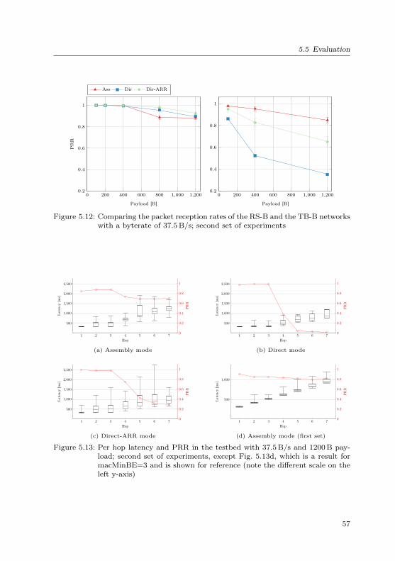
5.5 Evaluation
0 200 400 600 800 1,000 1,2000.2
0.4
0.6
0.8
1
Payload [B]
PR
R
Ass Dir Dir-ARR
0 200 400 600 800 1,000 1,2000.2
0.4
0.6
0.8
1
Payload [B]
Figure 5.12: Comparing the packet reception rates of the RS-B and the TB-B networkswith a byterate of 37.5 B/s; second set of experiments
0
0.2
0.4
0.6
0.8
1
PR
R
1 2 3 4 5 6 7
500
1,000
1,500
2,000
2,500
Hop
Late
ncy
[ms]
(a) Assembly mode
0
0.2
0.4
0.6
0.8
1
PR
R
1 2 3 4 5 6 7
500
1,000
1,500
2,000
2,500
Hop
Late
ncy
[ms]
(b) Direct mode
0
0.2
0.4
0.6
0.8
1
PR
R
1 2 3 4 5 6 7
500
1,000
1,500
2,000
2,500
Hop
Late
ncy
[ms]
(c) Direct-ARR mode
0
0.2
0.4
0.6
0.8
1
PR
R
1 2 3 4 5 6 7
500
1,000
Hop
Late
ncy
[ms]
(d) Assembly mode (first set)
Figure 5.13: Per hop latency and PRR in the testbed with 37.5 B/s and 1200 B pay-load; second set of experiments, except Fig. 5.13d, which is a result formacMinBE=3 and is shown for reference (note the different scale on theleft y-axis)
57

5 Basic Forwarding Techniques for 6LoWPAN-Fragmented Datagrams
Recall also that for the second set of experiments, the BEP for a frame was calculatedaccording to (4.1) in the physical layer model of the simulation.
Figure 5.12 shows the results for the second set of experiments. While the Assemblymode only had a slightly higher PRR compared to the first set of experiments, theDirect and Direct-ARR modes dramatically improved for the largest UDP packets byabout 0.4 and 0.13, respectively. Both performed better than the Assembly modein this regard. The decrease for payloads of 800 B can be explained by the reducedbuffer size used during the second set. The configuration allowed only a single 800 Bdatagram to fit the 6LoWPAN data buffer and therefore increases the number ofdrops.
Completely different are the results obtained from the testbed. Different fromthe simulation environment, the only property of the configuration changed was themacMinBe. Here, the Direct mode, though improved by 0.15, did not achieve an evencomparable PRR to that of the Direct-ARR mode. Then again, the Direct-ARR modedid not improve in comparison to the first set of experiments and achieves a muchlower PRR than the Assembly mode, which showed a very similar performance as inthe first set.
The latency plots obtained from the testbed (Fig. 5.13) showed an increase of themedian end-to-end latency for the Assembly mode in comparison to the first set ofexperiments (Fig. 5.13d), which was to be expected with the increased macMinBe.Also, the direct modes achieved better median latency values than the Assemblymode. However, the more striking observation was, that the PRR, while being near1 for the direct modes at nodes that are not more than three hops away from the thesink, dropped steeply for more distant nodes. For the plain Direct mode, the PRReven approaches 0 for nodes more that 5 hops distant from the sink. For Direct-ARR,the curve had a similar shape, but the decrease did not fall below 0.3 which is still adramatically bad performance.
A look at the reasons for dropped fragments revealed that for the Assembly mode,drops due to the lack of buffer space in the 6LoWPAN buffer was the primary reason,while for the direct modes, unsuccessful link-layer transmissions caused the majorityof packet losses.
The increase of macMinBe in the second set of experiments did not have the ex-pected effect in the testbed experiment. While the latency slightly increased, theoverall PRR did not improve by amounts comparable to the simulation environment.
5.5.3 Explanation of Results
At the time this first set of experiments was executed, we tried to explain the observeddifferences in results between simulation and testbed with the nature of the real worldenvironment:
• People were moving around constantly at daytime during the experiments.
• Numerous IEEE 802.11 hotspots, using the same ISM band may have causedadditional interference.
• The transient behavior of wireless links over time may have caused temporaldegradation of the link quality between pairs of nodes.
58
5.5 Evaluation
• The mechanism for time synchronization sporadically put an additional smallload on the real network.
In combination with the also degrading PRRs in simulation for the first set of exper-iments, which showed at least similar tendencies to the results from the testbed, theexplanation seemed reasonable. The stated reasons, however, fail to explain satisfac-torily, why the PRR of the Assembly mode deviates only slightly between simulationand testbed experiments.
Additionally, the PRR dropped to 0.5 and below 0.3 for the Direct mode in thetestbed environment in simulation and testbed, respectively. The average byterate ofthe traffic generator was equal in all experiments (λB = 37.5 B). Multiplying this valuewith the average path length in the RS networks results in an (lower bound) estimatefor the overall payload data rate of 1.08 kbit/s for the first and 1.176 kbit/s for thesecond set of experiments. These data rates are not terrifically high in comparisonto the IEEE 802.15.4 raw data rate of 250 kbit, even if CSMA/CA, header overheadand additional acknowledgments are considered. This does clearly not represent acongestion scenario. Therefore, the observed performance is unacceptably low.
This reasoning is supported by the fact that changing the BEP calculation in thesimulation and using a different macMinBe changed the results, in spite of the smaller6LoWPAN data buffer, while the testbed results remained virtually unchanged.
Another attempt to explain the results, especially of the second set of experiments,was to make the varying signal strength between retransmissions (drawing a newRSSI from a log-normal distribution; cf. Sect. 4.2.3) responsible for more successfultransmissions even in the presence of interference. We deemed this change of thecalculation of the BEP to be responsible for the simulation model underestimating theprobability of interference between frames leading to corrupted frames at the receivingnode(s) and thereby producing unrealistically good results. However, this explanationneglects the fact that in the testbed experiment, the change from macMinBe = 3 tomacMinBe = 5 did not lead to significantly different results.
The results clearly imply that the simulation model did not represent the realitysatisfactorily. A first attempt to get a better fit involved the introduction of a so-called decider correction factor (DCF). This DCF additionally attenuated the signalof an incoming frame by a certain value if interfering frames were present. Thereby,we wanted to increase the number of frames lost due to interference. This method didindeed decrease the overall PRR slightly, but the results were still completely differentfrom those obtained from the testbed.
I eventually identified the extended operating mode (Sect. 5.4.1) of the transceiver aspossible cause for the bad performance observed in the testbed. This mode is activatedby putting the transceiver into TX ARET state, which then automatically performsCSMA/CA backoffs, clear channel assessment and automatic retransmissions. In thisstate, the transceiver is not able to receive any incoming frames, which means thatit becomes “deaf” during the backoff phase. In Chapter 6, I examine the impact ofthis property and show that it is responsible for the vast majority of frame losses.This realization triggered the conduction of a revisited parameter study, which usedthe more accurate model for the bit error probability in simulation and a differentimplementation of the MacAbstractionLayer and is presented in Chapter 7.
In conclusion of the presented results, the major shortcoming of the presented ex-periment setup was the use of an inadequate formula for the BEP in the simulation
59

5 Basic Forwarding Techniques for 6LoWPAN-Fragmented Datagrams
environment (Sect. 5.4.2). It caused interfering frames to be lost with a probabilitynear 1 and – in contrast to the conclusions drawn then – overestimated the impact ofinterference in the real network. In combination with the unanticipated effects causedby the extended operating mode, simulation and testbed showed strikingly bad butseemingly plausible and consistent results. The execution of additional configurationsclearly showed that there existed some mismatch between testbed and simulationmodel. Therefore, the results presented in this chapter underline how important anaccurate simulation model and its validation are.
60

6 Hardware-Assisted IEEE 802.15.4Transmissions
In this chapter, the reasons for the difference between results from simulation andtestbeds as observed in Sect. 5.5 are examined. The realization of the transmissionin hardware, including the CSMA/CA mechanism, is identified as the culprit in thisregard.
6.1 Hypothesis
Possible reasons for the pronounced differences between Assembly and Direct modesare discussed in Sect. 5.5. However, these fail to explain, why for the Assembly modethe results from simulation and testbed are very similar, while they differ dramaticallyfor the Direct modes. Especially in the second set of experiments, which uses theformula to calculate the BER as given by the IEEE 802.15.4 standard, the differenceis large. One remaining significant distinction between simulation environment andtestbed is, that the protocol stack employed in the testbed makes use of Atmel’sATmega256RFR2 transceivers [14] extended operating mode.
This mode provides two additional basic states, RX AACK and TX ARET. En-tering the former state activates automatic acknowledgments, which are sent au-tonomously by the transceiver. Its counterpart is the TX ARET state, which enablesautomatic retransmissions for unicast frames. With TX ARET, the transceiver alsohandles the CSMA/CA protocol of IEEE 802.15.4, i.e., employs a backoff phase andclear channel assessment (and additional backoffs in case of busy channels). A similarautomatic mode of operation is found in Microchip’s MRF24XA [15]. Such hardware-assisted operating modes are compelling as they can reduce the complexity of theradio driver and link layer and potentially reduce the protocol stack’s program anddata memory1, the number of peripherals (timer) and the load on the CPU. Addi-tionally, the processing is faster that way and thereby can speed up the transmissionspeed of a frame. However, such extended operating modes deactivate the receptionof frames in TX ARET mode. In consequence, no frame can be received during thewhole backoff/CCA phase.
In a scenario with multiple hops and 6LoWPAN fragmentation, I expect this “no-RX-while-TX” property of the extended operating mode to be responsible for a largenumber of frame losses, especially using one of the Direct modes. With multipleframes being available for sending at once (due to fragmentation), on a multi-hoproute there is a high probability for consecutive frames to “interfere” in the sensethat a subsequent frame is transmitted while it predecessor frame is pending in TX -ARET state at the next-hop node. Figure 6.1 illustrates this situation for an extended
1Of the implementations described in Sect. 6.2, the AACK MAC is smaller than the SoftwareMAC by 5280 bytes ROM and 578 bytes RAM
61

6 Hardware-Assisted IEEE 802.15.4 Transmissions
2
1
2
1
no-Rx-while-TX
Time
· · ·
· · ·
RX-while-TX
Time
Node
IDLE RX TX BO RX TX PENDING TX RADIO
Figure 6.1: Example for sequence of states for two nodes on a multi-hop path leadingto the loss of a frame transceivers with “no-RX-while-TX”, while “RX-while-TX” transceivers receive all frames
operating mode (“no-RX-while-TX”) and a “RX-while-TX” implementation. In theformer case, a frame is sent repeatedly into the deaf next hop node, which performsconsecutive backoffs and therefore is unable to receive the frame until the sender givesup after a number of retransmissions. Goal of the experiments conducted in thischapter is to verify this assumption.
6.2 Capturing Node State in Real-Time
Three approaches can be applied to evaluate the extended operating modes’ impacton the overall performance:
• An analytical approach, based on a model similar to the one proposed by Lu-dovici et al. [Lud+14], but extended to a multi-hop scenario.
• A simulative approach, using a model which captures the behavior of such anextended operating mode.
• An approach comparing two implementations in a testbed, with the possibilityto capture the sequence of states of each node’s MAC layer.
I decided to adopt the third approach to be able to eliminate any inaccuracies andlimitations introduced by modeling the behavior. As representative for the extendedoperating mode, I use the MAC layer implementation for the ATmega256RFR2 that isincluded in CometOS (Sect. 4.1.3, [UWT12]). This implementation is called “AACKMAC” in the remainder of the thesis. As a reference, I ported the radio stack forthe ATmega128RFA1 (which is nearly identical to the ATmega256RFR2) of TinyOSto CometOS. The TinyOS radio stack was chosen, because it is widely used andmodularized. This layer implements the control of the transmission process comprisingacknowledgments, retransmissions, backoffs and clear-channel assessment in software.I also created an alternative backoff layer, which implements the unslotted CSMA/CAof 802.15.4 and replaces the default TinyOS backoff mechanism. This implementationis referred to as Software MAC throughout the thesis.
Keeping track of the accurate sequence of states of each node’s MAC layer posestwo major difficulties. First, the memory needed to store a large number of statechanges is not available on the resource-constrained nodes which already contain a
62

6.2 Capturing Node State in Real-Time
IDLE
TX BO
TX RF TX WAIT TX ACK
TX DONE
RXRX
RX DLRX DL RX ACKRX ACK
RX TX PDRX TX PD
RX DL TX PDRX DL TX PD
RX ACK TX PDRX ACK TX PD
RX DONE
RF TX END
TX START
RX DONE
RF
TX
END
RF
RX
END
TX BO FAIL
RX DONE
TXRET
RY
RF
RX
END
RX DONE,RX DROPPED
RF TX END
RX DONE
RFTXST
ART
RF
RX
START
TXBO
FAIL
TX START
RF
TX
END
RX DROPPED,RX DONE
TXRE
TRY
RF RX START
TX FAIL,TX SUCCESS
TXFA
IL,
TXSU
CCES
S
TX RETRY
RF RX DROPPED,RX DROPPED
RX
DON,RX
DROPPED,RF
RX
DROPPED
RF TX START
RF
RX
START
TX BO FAIL
RX DONE,RX DROPPED,
RF RX DROPPED
TX START
RF TX START
RF
RX
START
TX FAIL, TX SUCCESS,RX DROPPED, RX DONE
TXSTA
RT
RF RX START
IDLE RX TX BO RX TX PENDING TX RADIO
Figure 6.2: State machine for Software MAC
complete IPv6/6LoWPAN stack plus a parallel stack to control the execution of ex-periments. Secondly, time synchronization with the accuracy of some µs betweennodes is necessary to accurately interpret state sequences locally. To achieve sucha synchronization, additional frames on the wireless channel are necessary, interfer-ing with the data frames of the experiment. For those reasons, I pursued a differentapproach and instrumented both MAC layer implementations to encode all relevantevents as a 4 bit value and signal them to another microcontroller using plain GPIOports.
I decided to directly output the present event instead of keeping track of the com-plete state machine within a node throughout the different layers of the radio stack.This was done in order to make the instrumentation of code as non-intrusive as pos-sible. In consequence, only four CPU cycles (250 ns) are needed to update the valueof the GPIO port to signal a new event.
63
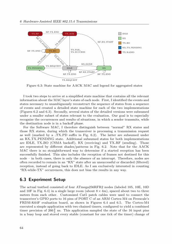
6 Hardware-Assisted IEEE 802.15.4 Transmissions
IDLE
TX BO
TX RF TX ACK
RXRXTX PENDINGTX PENDING
TXSTART T
XBOFA
IL
RF TX END
RFTXSTART
TX REQUEST
RX DONE
RF TX END
RF TX END
TXRETRY
RF RX START
TX FAIL,TX SUCCESS
TX REQUEST
RF RX STARTRF TX END
IDLE
RX
TX BO
RX TX PENDING
TX RADIO
Figure 6.3: State machine for AACK MAC and legend for aggregated states
I took two steps to arrive at a simplified state machine that contains all the relevantinformation about the MAC layer’s state of each node. First, I identified the events andstates necessary to unambiguously reconstruct the sequence of states from a sequenceof events and created a detailed state machine for each of the two implementations(Figures 6.2 and 6.3). Secondly, several states of the detailed versions were subsumedunder a smaller subset of states relevant to the evaluation. Our goal is to especiallyrecognize the occurrences and results of situations, in which a sender transmits, whilethe destination node is in a backoff phase.
For the Software MAC, I therefore distinguish between “normal” RX states andthose RX states, during which the transceiver is processing a transmission requestas well (marked by a TX PD suffix in Fig. 6.2). The latter are subsumed underan RX TX PENDING state. Additional subsumed states for both implementationsare IDLE, TX BO (CSMA backoff), RX (receiving) and TX RF (sending). Thoseare represented by different shades/patterns in Fig. 6.2. Note that for the AACKMAC there is no straightforward way to determine if a started reception has beensuccessfully finished. This also includes the reception of frames not destined for thisnode – in both cases, there is only the absence of an interrupt. Therefore, nodes areoften recorded to remain in an “RX” state after an unsuccessful or discarded (filtered)reception, instead of going back to IDLE. As I am exclusively interested in counting“RX-while-TX” occurrences, this does not bias the results in any way.
6.3 Experiment Setup
The actual testbed consisted of four ATmega256RFR2 nodes (labeled 105, 10E, 10Dand 10F in Fig. 6.4) in a single large room (about 8× 4m), spaced about two to threemeters from each other. Customized Cat5 patch cables were used to connect thetransceiver’s GPIO ports to 16 pins of PORT C of an ARM Cortex-M4 on Freescale’sFRDM-K64F evaluation board, as shown in Figures 6.4 and 6.5. The Cortex-M4executed a simple application with two chained timers, configured to yield a combinedtimer precision of 266 2
3ns. This application sampled the state of the 16 input pins
in a busy loop and stored every stable (constant for one tick of the timer) change of
64

6.3 Experiment Setup
10F 10D
10E
105
RaspPi FRDM-K64F
PC Basestation
PC
Ethernet/TCP
UART
UART
Radio Link/Static Route
GPIO connection cable
Figure 6.4: Schematic diagram of experimental setup
Figure 6.5: Wireless and sampling nodes, and Raspberry Pi controller of experiment
65
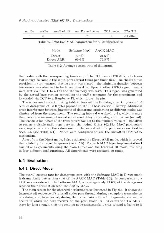
6 Hardware-Assisted IEEE 802.15.4 Transmissions
minBe maxBe csmaBackoffs maxFrameRetries CCA mode CCA TH
5 8 5 7 0 -90 dBm
Table 6.1: 802.15.4 MAC parameters for all configurations
Mode Software MAC AACK MAC
Direct 97 % 21.6 %Direct-ARR 99.6 % 79.5 %
Table 6.2: Average success rate of datagrams
their value with the corresponding timestamp. The CPU ran at 120 MHz, which wasfast enough to sample the input port several times per timer tick. The chosen timerprecision, in turn, ensured that no event was missed – the minimum duration betweentwo events was observed to be larger than 4 µs. Upon another GPIO signal, resultswere sent via UART to a PC and the memory was reset. This signal was generatedby the actual base station controlling the traffic generator for the experiment andforwarded via TCP to a Raspberry Pi, which drove the pin.
The nodes used a static routing table to forward the IP datagrams. Only node 105sent 20 datagrams of 1200 bytes payload to the PC base station. Thereby, additionalcross-interference between fragments of datagrams originating at different nodes waseliminated from the experiment. The sending interval was fixed to 4 s, which is morethan twice the maximal observed end-to-end delay for a datagram to arrive (or fail).The transmission power of the transceivers was set to the minimal value of −16.5 dBmto realize multiple radio hops between the nodes. Other 802.15.4 MAC parameterswere kept constant at the values used in the second set of experiments described inSect. 5.5 (see Table 6.1). Nodes were configured to use the unslotted CSMA-CAmechanism.
Apart from the Direct mode, I also evaluated the Direct-ARR mode, which improvedthe reliability for large datagrams (Sect. 5.5). For each MAC layer implementation Icarried out experiments using the plain Direct and the Direct-ARR mode, resultingin four different configurations. All experiments were repeated 50 times.
6.4 Evaluation
6.4.1 Direct Mode
The overall success rate for datagrams sent with the Software MAC in Direct modeis dramatically better than that of the AACK MAC (Table 6.2). In comparison to a97 % success rate with the Software MAC, on average, only 21.6 % of the datagramsreached their destination with the AACK MAC.
The main reason for the observed performance is illustrated in Fig. 6.6. It shows the(aggregated) sequence of states all nodes pass through during a complete transmissionof a datagram. As expected, during the transmission of the 18 fragments, a situationoccurs in which the next receiver on the path (node 0x10E) enters the TX ARETstate for long enough, that the sending node unsuccessfully tries to send a frame to it
66

6.4 Evaluation
4000 4060 4120 4180 4240 4300 4360 4420 4480 4540 4600
0x105
0x10e
0x10d
0x10f
Time [ms]
Node
IDLE RX TX BO RX TX PENDING TX RADIO
Figure 6.6: Sequence of states; AACK MAC, Direct mode, run 0, datagram 1
0 45 90 135 180 225 270 315 360 405 450
0x105
0x10e
0x10d
0x10f
Time [ms]
Node
IDLE RX TX BO RX TX PENDING TX RADIO
Figure 6.7: Sequence of states; Software MAC, Direct mode, run 0, datagram 0
(recall that during TX ARET, the transceiver is unable to receive any frame). Thispattern can be observed in slight variations for most of the datagrams in all runs forthe AACK MAC in Direct mode.
The Software MAC’s superior performance can be mainly attributed to the differentbehavior concerning the reception of frames while being in some TX state (Fig. 6.7).The occasions in which a node received frames while being in a back-off state forit’s own transmission are marked as RX TX PENDING in the plot. It can be seenthat allowing these receptions of frames does not lead to any losses of frames pendingfor transmission, but on the contrary significantly reduces the number of necessaryretransmissions for the sending node.
Departing from individual datagrams to a more general view, the number of frag-ments in certain combinations of events at the sending node and state at the receivingnode were extracted from the experiment data. Table 6.3 shows the summed up andaveraged results for the first two nodes of the path (105, 10E).
Comparing these data, it can be observed that the number of total fragments sent(fragRequests) reaches only 57.7 % of the number of fragments needed for a com-plete transmission (fragRequests (max)) of the datagram, because often senders hadto give up the transmission due to a completely failed transmission of a fragment.
67

6 Hardware-Assisted IEEE 802.15.4 Transmissions
Software MAC AACK MAC
(0) fragRequests (theo. max) 720.00 720.00(1) fragRequests 717.10 99.6 % of (0) 415.30 57.7 % of (0)
(2) fragSuccessDstTx 518.48 0(3) fragSuccessDstNonTx 198.38 398.76(4) fragFailDstTx 81.96 13.6 % of (7) 423.08 100.0 % of (7)(5) fragFailDstNonTx 23.44 10.6 % of (8) 4.44 1.1 % of (8)(6) fragFailTotal 105.40 14.7 % of (1) 427.52 102.9 % of (1)
(7) fragDstTxTotal 600.44 423.08(8) fragDstNonTxTotal 221.82 403.20
Table 6.3: Average fragment counts of Software MAC and AACK MAC over 50 runs;Direct forwarding mode
Furthermore, there is a difference in the relative and absolute number of retries andtransmission failures caused by frames that were transmitted to a sender that was insome TX state (TX BO or TX RF), denoted as fragFailDstTx. For the AACK MAC,nearly all (99 %) failed frame transmissions are caused by such frames, compared to77.8 % for the Software MAC. Also, for the Software MAC, the ratio of failed transmis-sions with receiver-TX and receiver-non-TX states (fragFailDstNonTx) against theirrespective totals (fragDstTxTotal, fragDstNonTxTotal) are not far apart from eachother: 13.6 % vs. 10.6 %. This suggests that the probability of a successful transmis-sion is only slightly higher if the receiving node is in an idle state for the SoftwareMAC. Possible explanations for this small difference are:
• A Transmission started during a CCA by the receiver is lost with the usedimplementation (during CCA, SHR detection is disabled).
• Sender and receiver perform their CCA at nearly the same time and both startsending.
Much more pronounced is the overall number of failures, which is only 14.7 % ofthe total number of transmission requests for the Software MAC, but 102.9 % for theAACK MAC. This means that, using the AACK MAC, on average there is about oneretransmission for every initial transmission request.
Finally, a higher percentage of fragFailDstNonTx for the Software MAC over theAACK MAC (10.6 % vs 1.1 % of all fragments with the receiver in a non-TX state)is observable. A possible explanation can be found in the fact that, with the Soft-ware MAC, on average more fragments reach the nodes farther down the path andthereby increase the number of collisions due the hidden terminal problem, which isnot captured by the selected metrics.
6.4.2 Direct-ARR Mode
Using adaptive rate restriction increases the average datagram success rate of theSoftware MAC slightly, that of the AACK MAC greatly (Table 6.2).
68

6.4 Evaluation
20000 20060 20120 20180 20240 20300 20360 20420 20480 20540 20600
0x105
0x10e
0x10d
0x10f
Time [ms]
Node
IDLE RX TX BO RX TX PENDING TX RADIO
Figure 6.8: Sequence of states; AACK MAC, Direct-ARR mode, run 0, datagram 5
8000 8060 8120 8180 8240 8300 8360 8420 8480 8540 8600
0x105
0x10e
0x10d
0x10f
Time [ms]
Node
IDLE RX TX BO RX TX PENDING TX RADIO
Figure 6.9: Sequence of states; AACK MAC, Direct-ARR mode, run 0, datagram 2
Figures 6.8 and 6.9 show the sequences of states with AACK MAC and Direct-ARR mode for a successful and an unsuccessful datagram transmission, respectively.Figure 6.8 illustrates how the additional delay of the Direct-ARR mode mitigatesthe risk of deaf receivers. However, due to the inherent random nature of the lengthof backoffs in 802.15.4 and random failures on the the wireless channel, the delaymechanism does not completely prevent situations, in which again the sender tries toget its fragment to a receiver in TX ARET state, as shown in Fig. 6.9.
Observing the results of 50 runs, I found that the by far dominating cause for lossesand retransmissions for the AACK MAC are again those fragments, which where lostdue to the sender being in TX ARET state (Table 6.4). As for the Direct mode,the number of transmission failures caused by a receiver-TX state is two orders ofmagnitude larger than that of transmission failures with a receiver-non-TX state.
However, the relative (in comparison to the number of fragments transmissionsrequested in total) and absolute number of transmission failures is greatly reducedby the Direct-ARR mode, from 427.52 (102.9 %) to 116.5 (17.6 %). Considering thesimple traffic scenario with a single sender and only four hops, the performance of theAACK MAC can still be regarded as disastrous, especially compared with the 99.9 %achieved by the Software MAC.
69

6 Hardware-Assisted IEEE 802.15.4 Transmissions
Software MAC AACK MAC
(0) fragRequests (theo. max) 720.00 720.00(1) fragRequests 719.92 99.99 % of (0) 661.62 91.90 % of (0)
(2) fragSuccessDstTx 87.80 12.20 % of (1) 0.00(3) fragSuccessDstNonTx 632.10 87.80 % of (1) 657.28(4) fragFailDstTx 16.72 16.00 % of (7) 114.80 100.00 % of (7)(5) fragFailDstNonTx 42.44 6.30 % of (8) 1.70 0.26 % of (8)(6) fragFailTotal 59.16 8.20 % of (1) 116.50 17.60 % of (1)
(7) fragDstTxTotal 104.52 114.80(8) fragDstNonTxTotal 674.54 658.98
Table 6.4: Average fragment counts of Software MAC and AACK MAC over 50 runs;Direct-ARR forwarding mode
Software MAC AACK MAC
Direct Direct-ARR Direct Direct-ARR
fragRequests 2.3 0.16 16.23 8.84
fragSuccessDstTx 6.4 4.64 na nafragSuccessDstNonTx 5.9 4.67 16.75 9.27
fragFailDstTx 3.8 1.93 14.58 6.84fragFailDstNonTx 2.7 5.88 0.64 0.82
Table 6.5: Confidence intervals of average fragment counts for all configurations
Most clearly, the effect of the rate restriction is shown by rows (7) and (8) of Ta-ble 6.4. Apart from preventing hidden-terminal collisions, it also reduces the numberof occasions during which senders transmit toward a receiver in TX state. Thereby, theoverall ratio of fragments sent during receiver-TX and fragments sent during receiver-non-TX is more than inverted for the Software MAC and significantly changed for theAACK MAC. Interestingly, the absolute number of fragments is nearly the same forboth MAC implementations (rows (7) and (8)).
Confidence intervals for all experiments were omitted for clarity from the resultstables and are shown in Table 6.5.
6.5 Conclusions
In this chapter, an experimental setup to analyze the sequence of events and statesof the MAC layer within a 6LoWPAN network was presented, focusing on the trans-mission of fragmented large datagrams with the cross-layered Direct and Direct-ARRmodes. The results of the experiments in a testbed of four nodes forming a simple linetopology have shown, that the extended operating mode of the hardware transceiveris responsible for the bad performance and the observed difference to the results fromsimulation. Additional mechanisms like rate restriction can significantly improve theperformance by preventing situations in which packet losses typically occur, but an
70

6.5 Conclusions
implementation using the extended operating mode is still not competitive and biasesexperiment results significantly. Moreover, it does so in a rather devious way, whichis difficult to distinguish from hidden terminal collisions or random sources of frameloss, especially in cases where the reduction is less dramatic, e.g., for the Direct-ARRmode.
Although only a small testbed was evaluated, it is obvious that the degradation ofperformance can not be expected to be less severe in larger networks and/or networkswith a larger diameter. Application scenarios that involve consecutive transmissions ofmultiple frames along the same route employing an unslotted CSMA/CA mechanismtherefore should avoid using hardware-assisted transmissions in their current state.
This conclusion has triggered a revision of the experiments in Sect. 5.5 using theSoftware MAC, which is presented in Chapter 7. For the evaluation of the 6LoOFprotocol (Chapter 8), I also use the Software MAC implementation in the testbedexperiments.
71


7 Basis Forwarding Techniques Revisited – aParameter Study
In consequence of the results of the experiments described in Chapter 5 and Chap-ter 6, a parameter study with a configuration corresponding to the insights gainedwas conducted. This chapter introduces the new setup and configuration and presentsan evaluation for the forwarding modes Assembly, Direct and Direct-ARR. The maingoal of the evaluation is to identify a useful configuration of IEEE 802.15.4 parametersfor the 6LoOF evaluation.
7.1 Experiment and Simulation Setup
This section describes the configuration of testbed and simulation. I used the collectiontraffic pattern that was introduced in Sect. 5.4.4. The total traffic amount was set to120 000 B in simulation and testbed to prevent the simulations, which explored a muchlarger parameter space, from running for too long due to a large number of runs. Theconfiguration of implementation specific parameters was not changed in comparison tothe one presented in Sect. 5.4.1 and hence the memory usage of Assembly and Directmode was nearly identical.
7.1.1 Testbed
For this parameter study, the Software MAC as described in Sect. 6.2 was employedin the testbed. A new testbed containing 13 nodes in rooms along the corridor on thefourth floor of our office building was installed. In comparison to the network usedfor the evaluation in Chapter 5, the position of nodes was slightly changed. Fig. 7.1shows a rough ground plan containing the location of all nodes. The nodes are dresdenelectronic deRFmega256-23T00 wireless transceiver modules, equipped with an AtmelATmega256RFR2. Apart from some additional minor functionality of the transceiver
0
100101 102
103104
105
106
107
108 109 10A10B
10C
Figure 7.1: Locations of TB-C nodes and routing tree of TB-C
73

7 Basis Forwarding Techniques Revisited – a Parameter Study
P tx,exp P tx,topo
6.5 dBm −0.5 dBm
Table 7.1: Transceiver transmission power for experiment and TopologyMonitor run
0 100 105
106
101 107
102104
109
10A108
103
10B10C
(a) RS-C, TB-C
0 1 2 3 4 5 6 7 8 9 10
(b) Chain-11
Figure 7.2: Network topologies for the parameter study
and twice as much program and data memory, this controller/transceiver system-on-chip is identical to the Atmel ATmega128RFA1 employed in earlier experiments(Sect. 5.4.1).
The routing topology (Fig. 7.2) of the TB-C network was obtained as describedin Sect. 4.2.3. As before, a different transmission power was used for the run of theTopologyMonitor and the actual experiment. These are shown in Table 7.1. All runsin the testbed were repeated five times.
7.1.2 Simulation
The actual parameter study was carried out in the simulation environment, becauseit took several days to weeks to execute the experiments with a significant number ofruns in the testbed. The parameter set employed in the simulations included that ofthe testbed experiments for validation, but further varies most IEEE 802.15.4 MACparameters, the size of the 6LoWPAN data buffer and the payload size. I examinedthe three surviving modes of operation Assembly, Direct and Direct-ARR.
Three network topologies were evaluated: a line topology and two different flavors ofthe RS-C network (Fig. 7.2). The links in the Chain-11 network are all configured withthe same link quality of RSSI = −50 dBm and no variance. The two RS-C networksuse the same routing tree but different link configurations. The two configurationsuse links obtained from the TopologyMonitor with the transmission power of P tx,exp
and P tx,topo , respectively. Hence, one configuration represents the configuration ofTB-C, the other the configuration that could be used in the testbed, if links would beless time-varying.
74

7.2 Validation of RS-C
Q BEmin BEmax macMaxCSMABackoffs r
1280 B 5 8 5 7
Table 7.2: IEEE 802.15.4 and 6LoWPAN configuration for validation experiments
RS-C2 TB-C
0.6
0.7
0.8
0.9
1.0
1.1
0.6
0.7
0.8
0.9
1.0
1.1
37.5
Bs −
175Bs −
1
50 200 800 1200 50 200 800 1200
LUDP [B]
PR
R
ModeAss
Dir
Dir-ARR
Figure 7.3: Validation experiment; Comparison of average PRR obtained from TB-Cand RS-C for two different application data rates. The results betweensimulation and testbed are largely consistent.
The simulation runs for validation of the testbed were repeated five times. Tofurther decrease the size of the confidence intervals while retaining viable runtimes,this number was increased to 15 for the larger-scale study.
7.2 Validation of RS-C
I used a subset of the parameter space to perform a validation of the simulation modelas shown in Table 7.2. The configuration of this validation experiment is shown inTable 7.2 for the 6LoWPAN buffer size Qand the IEEE 802.15.4 CSMA/CA configu-ration values macMinBe (BEmin), macMaxBe (BEmax) and macMaxCSMABackoffs,as well as the maximum number of retransmissions macMaxFrameRetries (r).
7.2.1 PRR
Figure 7.3 shows the PRR obtained from simulation and testbed runs averaged over allnodes against size of an individual UDP packet LUDP for the three different operatingmodes and two different (application traffic) byte rates. The same values are shownagain in Table 7.3 for exact reference. As a general result, it can be seen that simulation
75

7 Basis Forwarding Techniques Revisited – a Parameter Study
λB [B s−1] LUDP [B] Network PRRAssembly Direct Direct-ARR
37.5 800 TB-C 0.822 0.933 0.97637.5 800 RS-C 0.874 0.936 0.968
37.5 1200 TB-C 0.843 0.859 0.93437.5 1200 RS-C 0.870 0.860 0.891
75 800 TB-C 0.726 0.888 0.94675 800 RS-C 0.750 0.863 0.904
75 1200 TB-C 0.693 0.751 0.84775 1200 RS-C 0.743 0.735 0.778
Table 7.3: Validation experiment; average PRR values for the two largest payloadsizes and different total byterate λB (rows) from simulation and testbed(columns) with comparable configuration.
and testbed results exhibit similar behavior. For the two largest payloads, the PRRdecreases significantly. This effect is more pronounced for the higher application datarate. For the Assembly mode with the two largest UDP payloads, a steep drop of thePRR can be observed from almost 1 to below 0.9 and 0.8 for a data rate of 37.5 Band 75 B, respectively. Both simulation and testbed show the Direct-ARR modeperforming best for large datagrams. The plain Direct mode achieves nearly identicalvalues in simulation and testbed, regardless of the configuration setting.
All modes consistently reach a PRR of almost 1 for UDP payloads of 200 B, while thePRR for 50 B packets is significantly lower with the higher data rate in the simulation.At this point, the testbed results deviate from the simulation. The Direct mode showsnearly identical behavior, but Direct-ARR (with a very large confidence interval) andAssembly (reaching a PRR of nearly 1) are different in the testbed. In simulation, thedrop is caused by a lack of message structures used by 6LoWPAN and IPv6 layer tocommunicate, which cannot be observed in the testbed to the same extent, except forthe Direct-ARR mode.
For the scenarios evaluated, there is also a consistent bias in the results for theAssembly and the Direct-ARR modes. The Assembly mode achieves an average PRRin simulation which is by 0.027 to 0.052 higher than the corresponding results fromthe testbed. In contrast, the Direct-ARR mode consistently achieves a 0.012 to 0.069higher PRR in the testbed. In consequence, the Direct-ARR outperforms the Assem-bly mode by a significantly larger margin in the testbed for the given settings.
7.2.2 Drop Causes – 6LoWPAN Layer
Analyzing the causes for dropped datagrams shown in Fig. 7.4 for the higher of theevaluated data rates and UDP payloads of 1200 B, it can be observed that generaltrends again can be observed in testbed and simulation. The vast majority of dropsin Assembly mode is caused by a lack of space in the data buffer. Given a 6LoWPANbuffer size of Q = 1280 B, which forces the 6LoWPAN module to drop fragmentsif more than one datagram of those sizes is reassembled, this does not come as a
76

7.2 Validation of RS-C
RS-C2 TB-C
0.0
0.5
1.0
0.0
0.5
1.0
0.0
0.5
1.0
Ass
Dir
Dir-A
RR
100
105
106
101
107
102
104
108
109
10A
103
10B
10C
avg
100
105
106
101
107
102
104
108
109
10A
103
10B
10C
avg
Node Id and avg
#da
tagram
s(norm)
dropReasonMacFail
BufferFull
Figure 7.4: Drop causes for each node and average for the whole network, normalizedby the total number of UDP packets transmitted per node. Data rate ofλB = 75 B s−1
surprise. It explains the steep drop of the PRR for the Assembly mode. The testbedresults show a slightly larger number of datagrams dropped due to failures at thelink layer compared to those obtained by simulation. The same can be stated for theDirect mode. While the overall PRR of the Direct mode is nearly identical, the ratioof drops due to link layer failures and due to lack of buffer space is nearly inversebetween testbed and simulation.
The Direct-ARR mode shows results different from Assembly and Direct mode: thenumber of link layer failures and the number of buffer drops in the testbed is smallerthan for the corresponding simulation environment.
In addition to these general observations, it can also be seen that the direct neighborof the basestation drops more datagrams due to link layer failures in the simulationenvironment than in the testbed. This is a direct cause of modeling this last hopas wireless link, in contrast to the testbed which uses a serial connection that is notgoverned by the CSMA/CA algorithm and exposed to interference by other node’stransmissions.
7.2.3 Drop Causes – Link Layer
A closer look at the causes for drops by the IEEE 802.15.4 link layer reveals thatfor all examined network topologies a consecutively failed CCA is responsible for thelargest share of drops. Figure 7.5 shows the data for the RS-C2 network and thecorresponding TB-C. Again, the general trend observed in the simulation is confirmedby the testbed experiment: Direct and Direct-ARR lose considerably more datagramsdue to drops at the link layer than Assembly. However, while in the simulated RS-C2
77

7 Basis Forwarding Techniques Revisited – a Parameter Study
RS-C2 TB-C
0
1
2
0
1
2
37.5
Bs −
175Bs −
1
Ass Dir Dir-ARR Ass Dir Dir-ARR
Mode
#fr
ames
(nor
m) retries
#retries6
#retries7
#CCA_fail
#fail
Figure 7.5: Causes of drops at the IEEE 802.15.4 link layer averaged over all nodes,normalized by the total number of UDP packets transmitted per node forsimulated and testbed networks (columns) and total byterate λB (rows).Additionally the number of frames with a large number of frame retrans-missions is shown.
network frames are dropped exclusively due to CSMA/CA failures, in TB-C, frameswere also dropped because the maximum number of retransmissions is reached. Notethat this can be implicitly deduced from the fact that numCSMAFails is smaller thanthe numOutgoingNotAcknowledged metric. The number of retransmissions for eachframe has not been recorded in the testbed during this evaluation and is depicted as 0in the plot, while for the simulation environment the depicted 0 represents the actualnumber of frames with a corresponding number of retransmissions.
The fact that CSMA/CA drops are the sole reason for frame drops in the simulationalso explains the surprisingly large number of frames dropped by the link layer at thebasestation-attached node: The excellent link quality installed between the two nodesdoes not save it from CSMA/CA failures.
Additionally, large confidence intervals can be observed for the total number offrames dropped in the testbed experiments for the higher data rate. With the confi-dence intervals for drops caused by buffer drops being comparatively smaller, it can bededuced that the number of drops due to consecutively failed link layer retransmissionsvaries strongly between runs.
These results shed some more light on the behavior of the overall PRR betweensimulation and testbed. For both data rates, the testbed drops significantly moreframes after the maximum number of link layer retransmissions. The arguments statedin Sect. 5.5.3 enumerating reasons for frames losses in the testbed, while not logicallysound for the results in that section, provide a possible explanation for the effectobserved here.
78
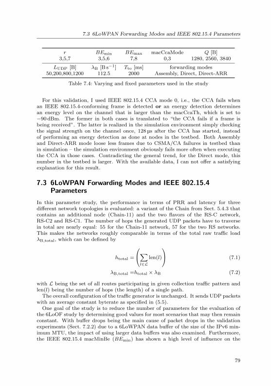
7.3 6LoWPAN Forwarding Modes and IEEE 802.15.4 Parameters
r BEmin BEmax macCcaMode Q [B]3,5,7 3,5,6 7,8 0,3 1280, 2560, 3840
LUDP [B] λB [B s−1] Tto [ms] forwarding modes50,200,800,1200 112.5 2000 Assembly, Direct, Direct-ARR
Table 7.4: Varying and fixed parameters used in the study
For this validation, I used IEEE 802.15.4 CCA mode 0, i.e., the CCA fails whenan IEEE 802.15.4-conforming frame is detected or an energy detection determinesan energy level on the channel that is larger than the macCcaTh, which is set to−90 dBm. The former in both cases is translated to “the CCA fails if a frame isbeing received”. The latter is realized in the simulation environment simply checkingthe signal strength on the channel once, 128 µs after the CCA has started, insteadof performing an energy detection as done at nodes in the testbed. Both Assemblyand Direct-ARR mode loose less frames due to CSMA/CA failures in testbed thanin simulation – the simulation environment obviously fails more often when executingthe CCA in those cases. Contradicting the general trend, for the Direct mode, thisnumber in the testbed is larger. With the available data, I can not offer a satisfyingexplanation for this result.
7.3 6LoWPAN Forwarding Modes and IEEE 802.15.4Parameters
In this parameter study, the performance in terms of PRR and latency for threedifferent network topologies is evaluated: a variant of the Chain from Sect. 5.4.3 thatcontains an additional node (Chain-11) and the two flavors of the RS-C network,RS-C2 and RS-C1. The number of hops the generated UDP packets have to traversein total are nearly equal: 55 for the Chain-11 network, 57 for the two RS networks.This makes the networks roughly comparable in terms of the total raw traffic loadλB,total, which can be defined by
htotal =
∑l∈L
len(l)
(7.1)
λB,total =htotal × λB (7.2)
with L being the set of all routes participating in given collection traffic pattern andlen(l) being the number of hops (the length) of a single path.
The overall configuration of the traffic generator is unchanged. It sends UDP packetswith an average constant byterate as specified in (5.5).
One goal of the study is to reduce the number of parameters for the evaluation ofthe 6LoOF study by determining good values for most scenarios that may then remainconstant. With buffer drops being the main cause of packet drops in the validationexperiments (Sect. 7.2.2) due to a 6LoWPAN data buffer of the size of the IPv6 min-imum MTU, the impact of using larger data buffers was also examined. Furthermore,the IEEE 802.15.4 macMinBe (BEmin) has shown a high level of influence on the
79

7 Basis Forwarding Techniques Revisited – a Parameter Study
2560B 3840B
0.50
0.75
1.00
0.50
0.75
1.00
0.50
0.75
1.00
Chain-11
RS-C
2R
S-C1
3 5 7 3 5 7
r
PR
R
ModeAss
Dir
Dir-ARR
Figure 7.6: PRR against r for different buffer sizes (cols) and networks (rows). Forthe shown cases, increasing r in all cases increases reliability. UDPpayload=1200 B, macCcaMode=3, BEmin=5, BEmax=8
overall reliability of transmissions in the initial study and is therefore examined forits default value and larger values. To get an indication if the macMaxBe (BEmax)has a similar influence, e.g., by shortening the overall transmission duration, a secondsetting is evaluated in this regard.
The analytical model presented in Sect. 3.2 indicates that a large number of retrans-missions successfully prevents rapidly decreasing end-to-end reliability, but is not ableto assess the influence of a large number of frame retransmissions on collision prob-abilities or the utilization of buffer space. The macMaxFrameRetries (r) is varied toevaluate the impact of this parameter.
Although macMaxCSMABackoffs was set to the allowed maximum value accordingto IEEE 802.15.4, the majority of frames were dropped because of a failed CSMA/CAprocedures. Therefore, an alternative IEEE 802.15.4 CCA mode (four different vari-ants are specified) (CCA) was evaluated. The CCA mode 0 was employed in theexperiments presented in Chapters 5 and 7. It corresponds to “Detection of a sig-nal with the modulation and spreading characteristics of this standard” OR “Energyabove the threshold” of the IEEE 802.15.4 standard [11a]. macCcaMode=3 changesthe logical operator between the two conditions to an “AND” and thereby increasesthe aggressiveness of the CCA, which is expected to lead to less failed CSMA/CAprocedures.
An overview of all settings is given in Table 7.4. For each configuration, 15 runswere executed, yielding a total of 19440 (1296 parameter combinations) runs for eachnetwork.
80

7.3 6LoWPAN Forwarding Modes and IEEE 802.15.4 Parameters
Ass Dir Dir-ARR
0
300
600
900
0
300
600
900
0
300
600
900
Chain-11
RS-C
2RS-C
1
3 5 7 3 5 7 3 5 7
r
#da
tagram
s dropReasonMacFail
BufferFull
OutOfHandlers
OutOfMessages
Figure 7.7: Drop causes against r for the different networks and forwarding modes.The number of drops due to lack of buffer space increase slightly for RSnetworks, but the overall number of drops decreases with increasing r
7.3.1 macMaxFrameRetries
First, the influence of the maximum number of frame retransmissions on the PRR isexamined. In all cases, a larger number of maximum frame retransmissions increasesthe average PRR in most network/parameter combinations. In the worst case, thePRR stays constant, which is the case for the RS-C2 network with macCcaMode0, because the sole reason for the dropping of frames is a failure of the CSMA/CAmechanism (cf. Sect. 7.2.3). This is exemplarily shown in Fig. 7.6. The Chain-11network achieves a PRR of almost 1 with the maximum value for r = 7 as specifiedby IEEE 802.15.4. RS-C2 and RS-C1 also benefit from a larger r.
Figure 7.7 additionally shows the drop causes for the same configuration and fora 6LoWPAN buffer size Q = 2560 B. Although the number of buffer drops slightlyincreases with increasing r, this effect is more than compensated by a decreasingnumber of drops at the link layer.
In conclusion, there was no configuration for which allowing more frame retrans-missions caused a decrease of the overall PRR. This observation is consistent with theanalytical model. Considering that the routes in our setup are static, this result is inline with my expectations. In consequence, the parameter r from is set to r = 7 forthe remaining evaluation.
81

7 Basis Forwarding Techniques Revisited – a Parameter Study
1280B 2560B 3840B
0.50
0.75
1.00
0.50
0.75
1.00
0.50
0.75
1.00
Chain-11
RS-C
2R
S-C1
3 5 6 3 5 6 3 5 6
BEmin
PR
R
ModeAss
Dir
Dir-ARR
Figure 7.8: PRR against BEmin for different buffer sizes (cols) and networks (rows).LUDP = 1200 B
7.3.2 macMinBe
The minimum backoff exponent of the unslotted CSMA/CA of IEEE 802.15.4 is ex-pected to have a large influence of the overall performance. Especially in multi-hopscenarios, a larger setting decreases the probability of self-interference between con-secutive 6LoWPAN fragments (cf. Sect. 5.5.2). First, the results are discussed for aLUDP = 1200 B, BEmax = 8 and macCcaMode = 0.
As can be seen, both Direct modes benefit by the BEminincreasing from 3 to 5(Figure 7.8). In contrast, the Assembly mode, which is much more prone to bufferdrops, does only achieve a higher PRR for the larger Q analyzed. With the smallestbuffer, the PRR even decreases significantly with increasing BEmin. For the givenconfiguration, the Direct-ARR mode shows the best results in the RS networks forBEmin = 5. With BEmin ∈ [3, 6], the PRR is lower. The PRR achieved by plainDirect mode, on the other hand, further increases for BEmin = 6 and the effect ismore strongly pronounced for larger values of Q.
A larger BEmin increases the probability for the Direct mode to avoid busy chan-nels and hidden-terminal collisions more often, whereas the Direct-ARR mode cannotfurther profit and even exhibits a decreased PRR. Note that the best PRR achievedby the Direct-ARR mode, however, is in the worst case only slightly lower (RS-C2,largest buffer) and otherwise slightly higher than the best result of the Direct mode.
The causes for drops (Fig. 7.9) reveal the issue that causes the Direct-ARR tolose more packets for BEmin = 6. The number of timeouts increases significantlyalthough the number of drops due to other reasons decreases in comparison to thesmaller BEmin. Note that the number of timeouts is difficult to interpret, becausea lost datagram will cause multiple (duplicate) timeout counting events: one at thenode where the datagram is initially lost and one at each node that has alreadyreceived at least one fragment belonging to that datagram. MAC failures and bufferdrops may also cause duplicate counting events, but for those cases already forwarded
82

7.3 6LoWPAN Forwarding Modes and IEEE 802.15.4 Parameters
Ass Dir Dir-ARR
0
500
1000
1500
2000
2500
0
500
1000
1500
2000
2500
0
500
1000
1500
2000
2500
Chain-11
RS-C
2RS-C
1
3 5 6 3 5 6 3 5 6
BEmin
#da
tagram
s
dropReasonMacFail
BufferFull
OutOfHandlers
OutOfMessages
Timeout
Figure 7.9: Drop causes against BEmin for different networks and forwarding modes.LUDP = 1200 B; Direct-ARR is still competitive to Direct, but suffersfrom the increasing number of timeouts (though no fragment is lost) forBEmin = 6
fragments have a good chance to be transported successfully to their final destination(and thereby not trigger another counting event of that kind). However, an increasingnumber of timeouts and a decreasing number of other drop causes at the same timeimply more datagrams have been dropped by a timeout event initially. With theAssembly mode, the ratio of other drop causes to timeouts is about 1; for everydropped datagram, the same datagram times out at the next hop node.
Especially for the idealized Chain-11 network, the Direct-ARR mode achieves asignificantly higher PRR for BEmin = 3. It can also be seen that this advantage ofthe Direct-ARR over the Direct mode, melts away with increasing BEmin, even whennot considering the large number of timeouts. On the other hand, in the comparison ofsimulation results and testbed experiment the Direct-ARR mode consistently achievedslightly better results (due to less MAC failures) in the testbed, while the Direct modelost more datagrams to MAC failures.
The PRR achieved by the Assembly mode with the largest examined buffer size(Q=3840 B) is best for BEmin = 5, regardless of the network topology. For BEmin =3, especially in the more complex RS networks, MAC failures can be observed, forBEmin = 6, buffer drops occur.
With BEmin = 6 achieving an only slightly better a PRR only for a small numberof cases and causing timeouts of datagrams for the Direct-ARR mode, I settle forBEmin = 5 as a compromise for following experiments and the 6LoOF evaluation.
83

7 Basis Forwarding Techniques Revisited – a Parameter Study
Figures 7.8 and 7.7 also provide some insight into the effect of the 6LoWPAN buffersize. Especially the Assembly mode benefits from larger buffers. Considering thatwith Assembly, whole datagrams have to be stored at intermediate nodes, this hasbeen expected. The Direct modes lose much less datagrams to buffer drops and hencebenefit less strongly from a larger buffer. Although nodes have to put the completeUDP payload into the 6LoWPAN buffer once the traffic generator generates a packet(and thereby also have to store 1200 B), even for the smallest buffer size the availablespace increases with each transmitted fragment. In general, the Direct modes copebetter with smaller buffers.
7.3.3 macCcaMode
1280B 2560B 3840B
0.60.70.80.91.0
0.60.70.80.91.0
0.60.70.80.91.0
Chain-11
RS-C
2R
S-C1
Ass Dir Dir-ARR Ass Dir Dir-ARR Ass Dir Dir-ARR
Mode
PR
R
macCcaMode0
3
Figure 7.10: PRR against forwarding mode; for different networks and buffer sizes,examining macCcaMode 0 and 3. macCcaMode0 performs better in com-plex scenarios with many weak links.
The impact of the macCcaMode strongly depends on the network topology underexamination. In the idealized Chain-11 network, the transmission and interferencerange is modeled comparable to a unit disc, where each node is within the com-munication radius of only the nodes next to it. Hence, the macCcaMode does notsignificantly change the results for that network. In contrast, the RS-C2 network usesa unnecessarily high transmission power, thereby increasing interference and trans-mission range far beyond the next hop node. In RS-C1, on the other hand, routes arechosen according to the transmission range.
Figure 7.10 shows the resulting PRR plot. In RS-C2, macCcaMode 3 consistentlyachieves higher PRRs than macCcaMode 0 for all modes and buffer sizes. In theRS-C1 network, the effect is inverted and macCcaMode 0 performs better.
The reason for the diametrical behavior is shown in Figure 7.11. In conformancewith the observations from the validation (cf. Sect. 7.2.3), the dominating cause forthe drop of datagrams at the MAC layer are continuously failing CCAs. The MAC
84

7.3 6LoWPAN Forwarding Modes and IEEE 802.15.4 Parameters
0 3
0
200
400
600
0
200
400
600
RS-C
2R
S-C1
Ass Dir Dir-ARR Ass Dir Dir-ARR
Mode
#fr
ames
retries#retries6
#retries7
#CCA_fail
#fail
Figure 7.11: Link layer drop causes against forwarding mode; for different RS networksand macCcaMode. The more defensive approach of macCcaMode 0 leadsto a large number of CSMA/CA backoff failures, the more aggressivemode 3 to more failures after unsuccessful retransmissions
drops the frame and thereby the datagram after macMaxCSMABackoffs CCA retries.In the RS-C2, the more aggressive macCcaMode 3 significantly reduces the numberof such CSMA/CA failures at the expense of a small increase of drops due to failedretransmissions.
For the RS-C1 network, a small share of the drops is caused by failed transmissionswith macCcaMode 0. With the more aggressive macCcaMode 3, there is only anegligible number of drops caused by CSMA/CA failures, but a significant increasein drops due to transmission failures can be seen. The latter effect overshadows theformer and hence the observed PRR can be explained.
RS-C1 represents the more realistic network topology, because a good routing pro-tocol will always try to find the shortest reliable routes. Therefore, I decide to usethe more defensive macCcaMode 0 in following experiments. This is also the modesupported by the radio driver used for the transceivers in the testbed.
The fact that RS-C2 with macCcaMode 3 outperforms RS-C1 with macCcaMode 0in terms of reliability, does not serve as an argument against mode 0, however. Ithas to be considered that higher transmission power does improve the reliability inabsence of interference and it also decreases the number of potential hidden terminalsin this network, because the diameter of the transmission range graph is much smallerthan that of routing graph. Therefore, the comparison is inherently unfair. A faircomparison should use routes that have been determined using the same transmissionpower, which is likely to decrease the resulting diameter of the routing graph as well.
Given the results of the more aggressive macCcaMode 3, it is possible that alower macCcaTh, e.g., −95 dBm improves the performance. With the Atmel AT-mega128RFA1, however, the employed macCcaTh of −90 dBm is the minimal possiblevalue already (cf. Sect. 4.2.3). Therefore, this possibility was not investigated.
85
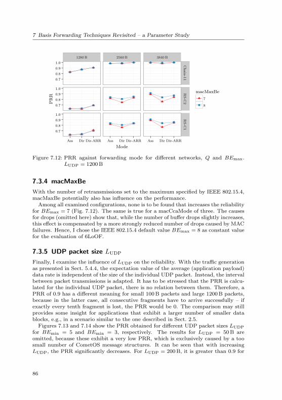
7 Basis Forwarding Techniques Revisited – a Parameter Study
1280B 2560B 3840B
0.70.80.91.0
0.70.80.91.0
0.70.80.91.0
Chain-11
RS-C
2R
S-C1
Ass Dir Dir-ARR Ass Dir Dir-ARR Ass Dir Dir-ARR
Mode
PR
R
macMaxBe7
8
Figure 7.12: PRR against forwarding mode for different networks, Q and BEmax.LUDP = 1200 B
7.3.4 macMaxBe
With the number of retransmissions set to the maximum specified by IEEE 802.15.4,macMaxBe potentially also has influence on the performance.
Among all examined configurations, none is to be found that increases the reliabilityfor BEmax = 7 (Fig. 7.12). The same is true for a macCcaMode of three. The causesfor drops (omitted here) show that, while the number of buffer drops slightly increases,this effect is compensated by a more strongly reduced number of drops caused by MACfailures. Hence, I chose the IEEE 802.15.4 default value BEmax = 8 as constant valuefor the evaluation of 6LoOF.
7.3.5 UDP packet size LUDP
Finally, I examine the influence of LUDP on the reliability. With the traffic generationas presented in Sect. 5.4.4, the expectation value of the average (application payload)data rate is independent of the size of the individual UDP packet. Instead, the intervalbetween packet transmissions is adapted. It has to be stressed that the PRR is calcu-lated for the individual UDP packet, there is no relation between them. Therefore, aPRR of 0.9 has a different meaning for small 100 B packets and large 1200 B packets,because in the latter case, all consecutive fragments have to arrive successfully – ifexactly every tenth fragment is lost, the PRR would be 0. The comparison may stillprovides some insight for applications that exhibit a larger number of smaller datablocks, e.g., in a scenario similar to the one described in Sect. 2.5.
Figures 7.13 and 7.14 show the PRR obtained for different UDP packet sizes LUDP
for BEmin = 5 and BEmin = 3, respectively. The results for LUDP = 50 B areomitted, because these exhibit a very low PRR, which is exclusively caused by a toosmall number of CometOS message structures. It can be seen that with increasingLUDP, the PRR significantly decreases. For LUDP = 200 B, it is greater than 0.9 for
86

7.3 6LoWPAN Forwarding Modes and IEEE 802.15.4 Parameters
1280B 2560B 3840B
0.70.80.91.0
0.70.80.91.0
0.70.80.91.0
Chain-11
RS-C
2R
S-C1
200 800 1200 200 800 1200 200 800 1200
LUDP [B]
PR
R
ModeAss
Dir
Dir-ARR
Figure 7.13: PRR against LUDP; different networks, Q and forwarding modes.BEmin = 5, BEmax = 8, macCcaMode = 0.
1280B 2560B 3840B
0.6
0.8
1.0
0.6
0.8
1.0
0.6
0.8
1.0
Chain-11
RS-C
2R
S-C1
200 800 1200 200 800 1200 200 800 1200
LUDP [B]
PR
R
ModeAss
Dir
Dir-ARR
Figure 7.14: PRR against LUDP; different networks, Q and forwarding modes.BEmin = 3, BEmax = 8, macCcaMode = 0
87
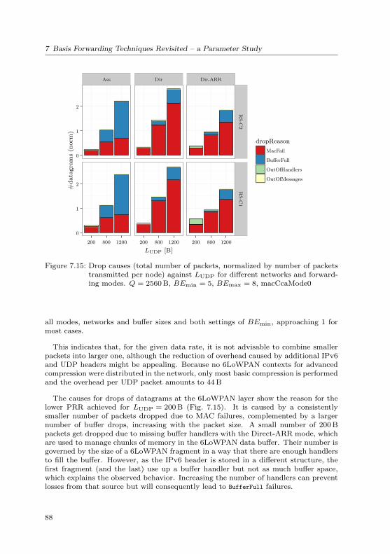
7 Basis Forwarding Techniques Revisited – a Parameter Study
Ass Dir Dir-ARR
0
1
2
0
1
2
RS-C
2RS-C
1
200 800 1200 200 800 1200 200 800 1200
LUDP [B]
#da
tagram
s(norm)
dropReasonMacFail
BufferFull
OutOfHandlers
OutOfMessages
Figure 7.15: Drop causes (total number of packets, normalized by number of packetstransmitted per node) against LUDP for different networks and forward-ing modes. Q = 2560 B, BEmin = 5, BEmax = 8, macCcaMode0
all modes, networks and buffer sizes and both settings of BEmin, approaching 1 formost cases.
This indicates that, for the given data rate, it is not advisable to combine smallerpackets into larger one, although the reduction of overhead caused by additional IPv6and UDP headers might be appealing. Because no 6LoWPAN contexts for advancedcompression were distributed in the network, only most basic compression is performedand the overhead per UDP packet amounts to 44 B
The causes for drops of datagrams at the 6LoWPAN layer show the reason for thelower PRR achieved for LUDP = 200 B (Fig. 7.15). It is caused by a consistentlysmaller number of packets dropped due to MAC failures, complemented by a largernumber of buffer drops, increasing with the packet size. A small number of 200 Bpackets get dropped due to missing buffer handlers with the Direct-ARR mode, whichare used to manage chunks of memory in the 6LoWPAN data buffer. Their number isgoverned by the size of a 6LoWPAN fragment in a way that there are enough handlersto fill the buffer. However, as the IPv6 header is stored in a different structure, thefirst fragment (and the last) use up a buffer handler but not as much buffer space,which explains the observed behavior. Increasing the number of handlers can preventlosses from that source but will consequently lead to BufferFull failures.
88

7.3 6LoWPAN Forwarding Modes and IEEE 802.15.4 Parameters
0
1000
2000
0
1000
2000
0
1000
2000
Ass
Dir
Dir-A
RR
1 2 3 4 5 6 7 8 9
Hops
Lat
ency
[ms]
(a) Chain-11
0
1000
2000
3000
4000
0
1000
2000
3000
4000
0
1000
2000
3000
4000
Ass
Dir
Dir-A
RR
1 2 3 4 5 6
Hops
Lat
ency
[ms]
(b) RS-C1
Figure 7.16: Latency against distance from sink (values accumulated for all nodeswith that distance); BEmin = 5, BEmax = 8, r = 7, macCcaMode0,Q = 2560 B
89
7 Basis Forwarding Techniques Revisited – a Parameter Study
7.3.6 Latency
I use a combination of violin and boxplot to depict the end-to-end latency. Theboxplots show median as horizontal bar and the lower and upper quartile as box. Thewhiskers represent the minimum or maximum values if these lie within 1.5 times theinter-quartile range; if not, the whiskers represent the most distant measured valuelying within 1.5 times the inter-quartile range. Values outside of this range are plottedindividually. The violin plots are cut at 1.5 times the inter-quartile range, too.
It can be seen that for the line topology, both Direct modes benefit from pipeliningand achieve a lower median latency than the Assembly mode at the most distantnode. The upper quartiles of both Direct modes are also lower than the median ofthe Assembly mode, which increases linearly with the distance. On the other and,the latency varies less with Assembly, even for nodes farther from the sink. Directand Direct-ARR show similar median values, but the inter-quartile range is larger forDirect-ARR.
For the RS-C1 network, the Assembly mode outperforms the Direct-ARR mode interms of median latency and again exhibits a smaller inter-quartile range. Latencies ofDirect and Assembly perform quite similar in all aspects. For this network topology,the Direct modes clearly cannot utilize the potential for pipelining.
7.3.7 Pull-Based Collection
A most simple alternative to push-based collection is a pull-based approach, i.e., thesink node polls every node in turn for its data. This approach, while arguably not avery sophisticated one, is attractive for a number of reasons:
• It is guaranteed that only one traffic flow is active at the same time. Interfer-ence does only occur between fragments of the same datagram and this can beprevented by using the Assembly mode.
• The overhead for sending an expectably small (fitting on IEEE 802.15.4 frame)request message becomes relatively small with the size of the data block re-quested. For example, with LUDP = 1200 B there is one small IEEE 802.15.4frame for the request and 18 large frames (fragments) for the data.
With a larger network diameter, the potential for parallel transmissions that do notinterfere with each other increases, but the overall total throughput is still boundedby one third of the throughput of a single link, because the last hop towards thesink always represents a bottle neck. To achieve a higher throughput, a push-basedapproach therefore needs to utilize the potential for parallel transmissions withoutbeing slowed down by interference between multiple flows.
To be able to quantitatively compare these approaches, additional experiments wererun. For those, the basestation/sink requests the transmission of an 1200 B data blockfrom all nodes in a round-robin fashion by means of a very small (2 B) CoAP message.The sink always waits for the current datagram to complete or a timeout of 3 s tooccur before it requests the next one. For 100 runs, the average duration of collecting200 data blocks from all nodes and the total PRR was recorded.
The results show that the Assembly mode achieves the fastest average collectiontime for the RS networks. A possible explanation can be found in the fact that
90

7.4 Summary
10000
10500
11000
11500
Ass Dir Dir-ARR
Mode
colle
ctio
nti
me
[ms]
Network RS-C2 RS-C1
(a) Duration for one collection
0.85
0.90
0.95
1.00
RS-C2 RS-C1
NetworkP
RR
ModeAss
Dir
Dir-ARR
(b) PRR of data collection
Figure 7.17: Collection duration and PRR for pull-based approach for the two RSnetworks
the Direct modes have a PRR below one, which means that the sink has to waitfor a timeout occasionally. This increases the overall duration. However, thoughDirect-ARR achieves a better PRR than the Direct, its duration for one collection islarger.
Using the average duration for 200 UDP packets with Assembly in the RS-C1network as reference (10 673.6 ms) yields an average payload data rate of approx.112.4 B s−1. This rate is all but equal to the data rate used for the push-basedcollection traffic scenario examined in this chapter (112.5 B s−1). The PRR of thepull-based collection with Assembly is almost 1 and hence it outperforms all RS net-work configurations of push-based collection examined in this chapter. Even arguingthat the used RS networks have a rather small diameter and comparatively mean linkcharacteristics, this has to be considered a rather bleak result.
7.4 Summary
Compared with the experiments presented in Chapter 5, the simulation and testbedsetup presented in this chapter produce results that match each other significantlybetter (cf. Sect. 7.2). Differences can be observed with regard to the causes fordropped frames at the 6LoWPAN layer and at the link layer. However, general trendsand effects can be observed in both environments and the results show the sametendencies, albeit not necessarily the same absolute numbers. Therefore, I deem thesimulation a viable tool to perform a large-scale parameter study and evaluation ofthe 6LoOF protocol (Sect. 8.4 and 7.3). Nevertheless, the conduction of testbedexperiments to re-validate simulation results is continued for evaluation of 6LoOF.
91

7 Basis Forwarding Techniques Revisited – a Parameter Study
r BEmax macCcaMode BEmin
7 8 0 5
Table 7.5: IEEE 802.15.4 MAC configuration parameters found to provide good per-formance for collection of large, 6LoWPAN-fragmented datagrams
The results of the conducted study have shown that there is a tremendous influenceof the configuration of the IEEE 802.15.4 MAC parameters on the reliability that canbe achieved in a multi-hop and multi-fragment collection traffic scenario.
For some parameters, it is possible to identify a setting that is beneficial for all ormost of the examined scenarios, others were more difficult to assess. macMaxBe andmacMaxFrameRetries clearly belong to the former, macCcaMode and macMinBe tothe latter category. To prevent parameter explosion (considering that 6LoOF comeswith its own set of parameters), I settled for the values shown in Table 7.5 for thefollowing experiments.
Furthermore, it can be stated that the Assembly mode performs well in terms ofreliability in the examined RS scenarios. Although being the most straightforwardimplementation, it is not impacted as strongly by the CSMA/CA or link layer trans-mission failures the Direct modes suffer from. With enough memory available for alarge 6LoWPAN data buffer, it outperforms both Direct modes in terms of reliability,even for BEmin = 6.
The behavior is different in the idealized Chain-11, for which the Direct-ARR modeoutperforms the other two modes. I assume that it benefits from the narrow inter-ference range, which only reaches to the adjacent node in the line topology, yieldingan average degree of two for the graph created by the “within interference range”relation. Hence, it can be assumed that the adaptive rate-restriction is able to pre-vent interference in many cases. In the RS-C2 and RS-C1 network, the degree ofthe link/interference graph is 11.85 and 11.15, respectively. This leads to more failedCCAs and retransmissions and thereby increases the variance of the average trans-mission duration T tx . Due to the EWMA smoothing, I expect the rate-restriction towork less effectively if the variance of T tx is large.
Examining a most simple pull-based collection approach, the superiority of thismethod compared a push-based collection with randomized transmission intervals hasbeen discovered for the examined network topologies and UDP packet sizes of 1200 B.In consequence, the evaluation of the 6LoOF protocol also considers data rates with thepotential for higher throughput than the corresponding pull-based collection approach.
92
8 6LoWPAN Ordered Forwarding - 6LoOF
This chapter introduces 6LoWPAN ordered forwarding, which was created as part ofthis doctoral thesis. The 6LoOF mechanism’s goal is to avoid the typical problemsencountered in the presence of 6LoWPAN fragmentation, as described in Chapter 7.
8.1 The 6LoOF Mechanism
All forwarding strategies presented in Sect. 7.3 (Assembly, Direct and Direct-ARR)exhibit packet reception rates significantly less than 100 %. The main reasons forthe packet drops are full forwarding buffers and consecutively failed clear channelassessments on the wireless channel in Assembly and Direct modes, respectively. Iassume that these losses in the Direct modes mainly occurred in situations in whichmultiple nodes try to forward large, fragmented datagrams within the same neigh-borhood, which resulted in increased channel contention and increased traffic volume,i.e., a local congestion. In consequence, an increased number of fragments and therebydatagrams were lost at the link layer in spite of repeated retransmissions.
6LoOF is an extension for direct forwarding that aims at reducing the number ofconcurrent transmissions in the immediate neighborhood of nodes. This is realized byutilizing the information provided by the 6LoWPAN fragmentation mechanism andadapting the rate at which nodes transmit their 6LoWPAN fragments. Simplisticallyspeaking, nodes that overhear their current next hop forwarding fragments belongingto a different datagram will completely stop the transmission of their current data-gram to allow for faster forwarding and less contention. As soon as transmission ofthe “foreign” datagram succeeded, the suspended transmission is reactivated. Thismechanism implements a congestion control with a narrow spatial and temporal scope.As it does not directly influence end-to-end sending rates, it does not prevent networkcongestion when the overall offered traffic is above the capacity of the network. Iexpect higher layers (TCP, CoAP) to deal with end-to-end congestion control.
This treatment of datagrams as traffic flows that suspend other traffic flows impliesthat nodes do not forward individual 6LoWPAN fragments using a FIFO approachas in the straightforward direct forwarding strategies. Instead, nodes always forwardwhole datagrams, i.e., they order incoming fragments by their belonging to a certaindatagram. Thus, the terms current next hop and active datagram here and in theremainder of the chapter describe the link layer destination of the datagram that iscurrently forwarded and this datagram itself, respectively. Note that with a route-overapproach, even using direct forwarding (cf. Sect. 2.2.3), this next hop does not changeduring transmission of a single datagram.
93

8 6LoWPAN Ordered Forwarding - 6LoOF
8.1.1 Snooping
6LoOF heavily relies on snooping of 6LoWPAN frames prefixed by a fragmentationheader to (re-) identify datagrams sent by other IPv6 routers. A node especially needsto identify transmissions of its current datagram originating at the current next hopfor this datagram. Using route-over forwarding, the datagram_tag changes with everywireless hop. In consequence it is necessary to combine IPv6 header information and6LoWPAN fragmentation header to achieve a reasonably accurate identification ofdatagrams. 6LoOF implements two different checks when it overhears a transmissionof its current next hop.
First, snooping the first fragment of a datagram, IPv6 header fields source anddestination are used for comparison. Note that the basic IPv6 header always fits thefirst fragment (cf. Sect. 2.2.1). Using the IPv6 header, the node can use destinationand source address along with the size of the datagram to check if the transmittedfragment is part of the node’s active datagram and thereby can decide whether to suc-ceed with its transmission or suspend it. The corresponding 6LoWPAN datagram_tag
is stored as metadata for the active datagram and is used to check further overheardfragments.
Secondly, if a FRAG N header is decoded without having a tag stored for thecurrent datagram, 6LoOF resorts to a sanity check. The fragment header’s size andoffset field are checked to determine if the overheard fragment may be part of theactive datagram, i.e., sizes have to be equal and the overheard offset smaller than thecurrent one for the fragment. Note that in case of false positives, this makes 6LoOFbehave similar to the corresponding non-6LoOF forwarding mode with regard to therate of transmissions.
For snooping to work, it has to be assumed that wireless links between nodes aresymmetric. All IEEE 802.15.4 unicast data traffic uses link-layer ACKs to confirm re-ception of a transmission, i.e., transmissions are only considered successful if a match-ing link-layer ACK is received. Routing protocols used above a IEEE 802.15.4 linklayer also have to consider that fact. Therefore, the assumption that wireless links aresymmetric between adjacent nodes in a routing graph is reasonable.
8.1.2 Probing
The general concept is illustrated in Fig. 8.1. Here, nodes A and B use node C as theirnext hop. Node C decides to forward the fragments of node A. This is overheard bynodes A and B (Fig. 8.1b). The former recognizes its active datagram and continuestransmitting fragments, the latter recognizes a different datagram and stops sending(Fig. 8.1c). Only after node B overhears the last fragment of A’s datagram (Fig. 8.1c),it enters state Sending again (Fig. 8.1d).
A problem with using a snooping-based approach is that in the absence of overheardframes, a node is not able to know if this absence is due to its next hop currentlysuspending its transmission or simply due to a random loss of frames on the wirelesschannel. In the latter case, nodes should continue transmitting to get a chance tosnoop from their successor. In the former case, however, it is not advisable to continuesending fragments to such a suspended node, as transmissions are likely to causehidden-terminal collisions at the suspended node. Figure 8.2 illustrates this issuewith node D being the suspended node. Furthermore, ACK frames sent from D to C
94
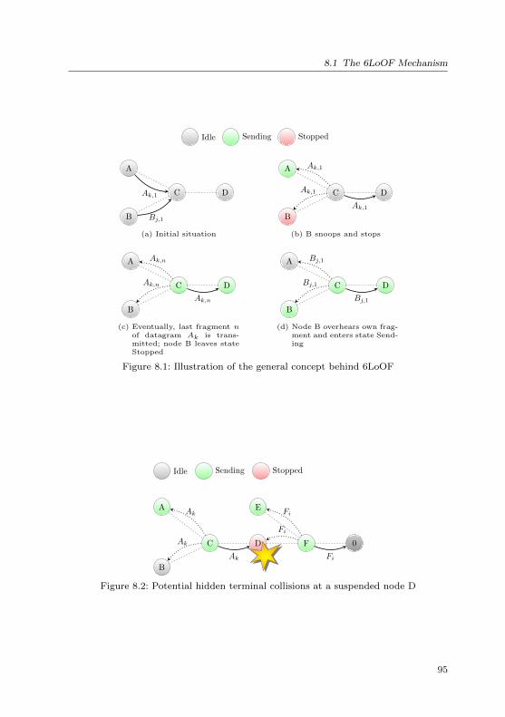
8.1 The 6LoOF Mechanism
Idle Sending Stopped
Ak,1
Bj,1
A
B
C D
(a) Initial situation
Ak,1
A
B
C D
Ak,1
Ak,1
(b) B snoops and stops
Ak,n
A
B
C D
Ak,n
Ak,n
(c) Eventually, last fragment nof datagram Ak is trans-mitted; node B leaves stateStopped
Bj,1
A
B
C D
Bj,1
Bj,1
(d) Node B overhears own frag-ment and enters state Send-ing
Figure 8.1: Illustration of the general concept behind 6LoOF
FiAk
Idle Sending Stopped
0
A
B
C D
E
F
Ak
Ak
Fi
Fi
Figure 8.2: Potential hidden terminal collisions at a suspended node D
95

8 6LoWPAN Ordered Forwarding - 6LoOF
Dispatch Header
11 010xxx FRAG1 EPN11 110xxx FRAG1 EPN
Table 8.1: Proposed header dispatch types to signal a node’s probing state (explicitprobing notification)
may also cause collisions at F with the traffic flow from E to F. In situations, in whichthere is more than a single sender, the suspended node’s buffer also has to store theincoming data without being able to empty it, up to a point at which the datagramhas to be dropped.
To mitigate this problem, a probing state for 6LoOF nodes is introduced. Nodes thatdo not snoop any fragment originating at their current next hop after a defined numberof sent fragments enter this state. Similar to the CSMA/CA protocol of IEEE 802.15.4,probing nodes exponentially reduce the frequency of their transmissions until they areable to snoop a fragment from the current next hop. Thereby, contention on thewireless channel is reduced if a confirming fragment was lost or the current next hopis suspended. Considering that the loss may also have been caused by a collision onthe wireless channel, reducing the rate of transmissions is a reasonable measure totake for both cases.
Additionally, nodes forwarding towards a probing node have no possibility to knowthat this node is probing. In consequence, such nodes will snoop a “probing” fragmentand if it matches their own datagram, will continue transmitting at a normal rate,governed solely by the rate restriction mechanism as described in Sect. 5.2.1. Toprevent nodes from transmitting to probing nodes at normal rate, additional headertypes for 6LoWPAN can be specified. These use the same format as FRAG 1 andFRAG N header of RFC 4944 ([Mon+07]), but a different dispatch to signal theprobing state of a node. The dispatch values are chosen from the reserved range ofdispatch values and do not interfere with any currently used dispatch values. Theyare shown in Table 8.1.
With the first draft of 6LoOF, preventing probing nodes to receive data at maximumrate was considered important enough to to justify an alteration of the 6LoWPANstandard headers. Reviewing this issue, it was concluded that sending to a probingnode at maximum rate is less harmful than thought initially. Given a routing topologythat tries to prevent unnecessarily long routes, a node that sends towards a probingnode is usually two hops away from the node in state Stopped that causes the nodeto probe. While this is by no means a guarantee that the stopped node is outside theinterference range of the sending node, there is a good probability that the strengthof potentially interfering signal is much lower than that of the fragments the stoppednode is trying to snoop. Therefore, the usage of these header dispatch types is optionalfor 6LoOF and is defined by the boolean parameter useEpnFlag xEPN. The impactof this parameter is examined in Sect. 8.4.1.
8.1.3 6LoOF Definition
Figure 8.3 on the following page shows a UML statechart defining the core of the6LoOF protocol.
96

Idle
entry/nswc=0entry/sendingAllowed=true
Active
Alive
entry/sendingAllowed=true
Sending
entry/probeFlag=false
Probing
entry/be= max(BE6LoOf,min+1, BE6LoOf,max)
Stalled
entry/sendingAllowed=falseexit/sendingAllowedCallback()
Stopped
entry/be= BE6LoOf,min
entry/scheduleStopTimer(e.fHdr)exit/cancelStopTimer()
ProbingBo
entry/scheduleProbeTimer(be)entry/probeFlag=trueexit/cancelProbeTimer()
6LoOF
SNOOP FOREIGN(e)/updateAv(e)
SENT(e)/nswc++;
[!checkAv(e.nH) && nswc ≤ NSWC max]/
[else]/be=BE6LoOf,min
SENT(e)/nswc++ [else]/be=BE6LoOf,min
[nswc <= NSWC max || nhIsDest(e.nH)]/
TIMERFIRED/
SENT(e)/
TIMER FIRED/
SNOOP1(e)/
[addressMatch(getActiveDg(),e.dg)]/setActiveTag(e.fHdr); nswc=0
[else]/
SNOOP N(e)/
[matchesActiveQo(e.fHdr)]/nswc=0
SNOOP1 EPN(e)/
[addressMatch(getActiveDg(),e.dg)]/setActiveTag(e.fHdr); be=BE6LoOf,min
SNOOPN EPN(e)/
[matchesActiveQo(e.fHdr)]/be=BE6LoOf,min
SENT LAST || SEND ABORTED || SWITCH QUEUE OBJ/
Figure 8.3: UML statechart – Core of the 6LoOF protocol
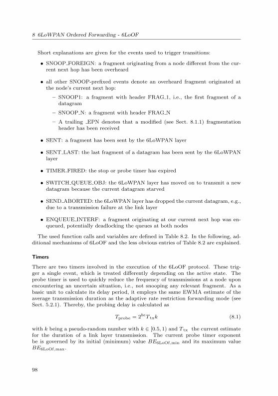
8 6LoWPAN Ordered Forwarding - 6LoOF
Short explanations are given for the events used to trigger transitions:
• SNOOP FOREIGN: a fragment originating from a node different from the cur-rent next hop has been overheard
• all other SNOOP-prefixed events denote an overheard fragment originated atthe node’s current next hop:
– SNOOP1: a fragment with header FRAG 1, i.e., the first fragment of adatagram
– SNOOP N: a fragment with header FRAG N
– A trailing EPN denotes that a modified (see Sect. 8.1.1) fragmentationheader has been received
• SENT: a fragment has been sent by the 6LoWPAN layer
• SENT LAST: the last fragment of a datagram has been sent by the 6LoWPANlayer
• TIMER FIRED: the stop or probe timer has expired
• SWITCH QUEUE OBJ: the 6LoWPAN layer has moved on to transmit a newdatagram because the current datagram starved
• SEND ABORTED: the 6LoWPAN layer has dropped the current datagram, e.g.,due to a transmission failure at the link layer
• ENQUEUE INTERF: a fragment originating at our current next hop was en-queued, potentially deadlocking the queues at both nodes
The used function calls and variables are defined in Table 8.2. In the following, ad-ditional mechanisms of 6LoOF and the less obvious entries of Table 8.2 are explained.
Timers
There are two timers involved in the execution of the 6LoOF protocol. These trig-ger a single event, which is treated differently depending on the active state. Theprobe timer is used to quickly reduce the frequency of transmissions at a node uponencountering an uncertain situation, i.e., not snooping any relevant fragment. As abasic unit to calculate its delay period, it employs the same EWMA estimate of theaverage transmission duration as the adaptive rate restriction forwarding mode (seeSect. 5.2.1). Thereby, the probing delay is calculated as
Tprobe = 2beT txk (8.1)
with k being a pseudo-random number with k ∈ [0.5, 1) and T tx the current estimatefor the duration of a link layer transmission. The current probe timer exponentbe is governed by its initial (minimum) value BE6LoOf,min and its maximum valueBE6LoOf,max.
98

8.1 The 6LoOF Mechanism
be probing exponent; to calculate backoff in probingstate
nswc number of fragments sent without snooping from cur-rent next hop
sendingAllowed output; denotes if 6LoOF allows sendingprobeFlag output; signals probing state to 6LoWPAN module
NSWC max 6LoOF parameter nNSWC,max
BE6LoOf,max 6LoOF parameter BE6LoOF,max
BE6LoOf,min 6LoOF parameter BE6LoOF,min
e.fHdr fragment information (size, offset, tag)e.nH IEEE 802.15.4address of current next hope.dg IPv6 datagram object
addressMatch() match IPv6 source and destination addressmatchesActiveQo() match by tag or sanity check (Sect. 8.1.1)
setActiveTag() attach received 6LoWPAN tag to active datagramgetActiveDg() returns the currently active IPv6 datagram (cf.
Sect. 8.1)nhIsDest() returns true, if current next hop equals the destina-
tion of the fragment
scheduleStopTimer() start timer to guarantee leaving state Stopped even-tually
scheduleProbeTimer() schedule probing backoffcancelStopTimer() stop the stop timer
cancelProbeTimer() stop the probe timer
checkAv() returns true, if a recent transmission from the currentnext hop has been overheard
updateAv() set or clear bit for neighbor based on snooped6LoWPAN frame
sendingAllowedCallback() signal 6LoWPAN layer that 6LoOF allows sendingthe next fragment
Table 8.2: Variables and actions (functions) used in the 6LoOF state machine
99
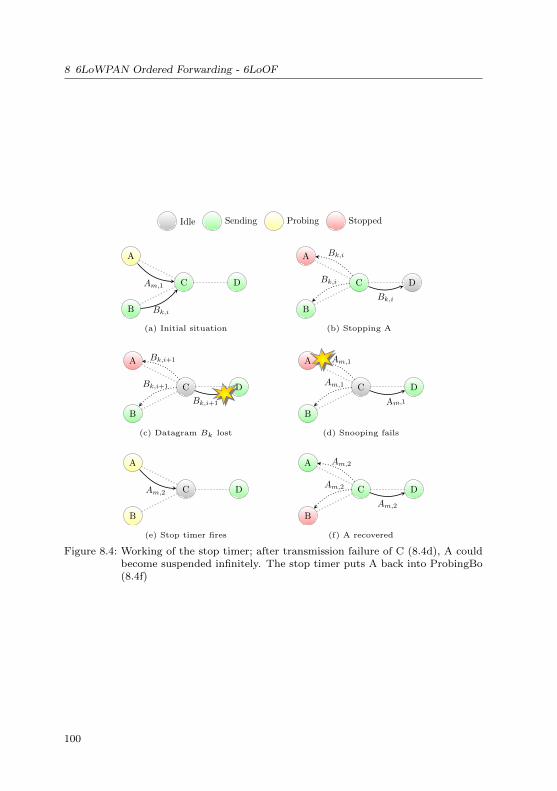
8 6LoWPAN Ordered Forwarding - 6LoOF
Idle Sending Probing Stopped
Am,1
Bk,i
A
B
C D
(a) Initial situation
Bk,i
A
B
C D
Bk,i
Bk,i
(b) Stopping A
Bk,i+1
A
B
C D
Bk,i+1
Bk,i+1
(c) Datagram Bk lost
Am,1
A
B
C D
Am,1
Am,1
(d) Snooping fails
Am,2
A
B
C D
(e) Stop timer fires
Am,2
A
B
C D
Am,2
Am,2
(f) A recovered
Figure 8.4: Working of the stop timer; after transmission failure of C (8.4d), A couldbecome suspended infinitely. The stop timer puts A back into ProbingBo(8.4f)
100
8.1 The 6LoOF Mechanism
The stop timer is necessary to prevent a node from being stuck in state Stopped.Consider the three nodes in Fig. 8.4. Node A entered state Stopped after snoopingfragment Bi,k. If datagram Bi is lost due to a buffer overflow or consecutively failingtransmissions at the link layer, node B will eventually stop sending fragments be-longing to it. In consequence, node A has no means to assess the situation withoutsnooping another fragment. One fragment of Aj has to be present at C, because Aalways transmits at least one fragment in probing state. However, there is no guar-antee that A successfully snoops such a fragment when it is transmitted by C. If nofragment is snooped, C starves while A is stuck in state Stopped. Therefore, a nodealways starts a timer upon entering state Stopped, with a duration of
Tstop =
datagram size−23datagram offsete.fHdr.size
T txkstop
2, (8.2)
T tx × kstop represents the average waiting time between forwarding two fragmentswith the Direct-ARR mode (Sect. 5.2.1). Tstop is half the estimated time it wouldtake this node to finish the transmission of the current next hop’s active datagram. Ifthis timer is triggered, the nodes enters state ProbingBo to transmit new fragmentsand eventually be able to snoop a confirming transmission.
Initial Transitions
Before some datagram arrives at a node, the node remains in state Idle. Anotherimportant decision concerns the state to enter upon sending the first datagram. Tosimplify this decision, nodes permanently monitor their neighborhood for transmis-sions. Ideally, a node stores information on individual transmissions of all neighbors,including the information necessary to calculate a stop timer delay as given in (8.2). Itcould then enter state Stopped directly without causing any interference to the ongo-ing transmission of its next hop. First, however, this would incur additional memorycosts (for at least datagram size and datagram offset), growing linearly with the sizeof the routing table, i.e., the number of potential next hops. Secondly, directly en-tering state Stopped denies a node the chance to leave this state by snooping one ofits own fragments (because it never sent any) in case its current next hop drops thedatagram that was responsible for letting the node enter state Stopped.
Therefore, 6LoOF only flags each entry in its routing table with an activity bit.updateAv() sets this bit if any FRAG N header is snooped that does not denote thelast fragment of a datagram, in which case the bit is cleared. Receiving an event SENTwith a node that is flagged active as next-hop destination, a node enters ProbingBoinstead. Note that this single-bit flag has a good chance to not occupy any additionalmemory, because an entry in a routing table usually contains a variable for prefixlength, which can be restricted to 7 bit (sensible prefix lengths are in the range [1, 128]).
If the current next hop is considered idle, the 6LoOF parameter “number sentwithout confirmation” (NSWC max) governs how long a node will stay in state Send-ing if it does not snoop its own fragments being forwarded by the current next hop.NSWC max specifies the number of fragments to transmit without such a confirmation(cf. Fig. 8.3).
101

8 6LoWPAN Ordered Forwarding - 6LoOF
Ak,1
Ak,2
Idle Sending Stopped
0
A
B
C D
E
F
Ak,1
Ak,1
Figure 8.5: Scenario leading to a node starving; new incoming datagrams are blockedat node F, because no new fragments arrive for datagram Ak, which is atthe head of the transmission queue
Prevention of Node Starving
Because 6LoOF forwards datagrams in an orderly fashion, a mechanism has been im-plemented to prevent nodes from “starving unnecessarily”. Different from the straight-forward direct modes, a node always tries to forward all fragments belonging to onedatagram before moving to another (Sect. 8.1). This property makes the idea of sus-pending transmissions viable in the first place. A fragment of datagram Ak that islost at a former node on the route, however, causes a node farther down the routeto block on that datagram. This is illustrated in Fig. 8.5, where node F is starvingafter transmission of Ak,1, because Ak,2 has been lost at C. The active datagram Akis at the head of the transmission queue at node F and no new fragments are goingto arrive. Note that node F has no way of knowing that the datagram Ak has beenlost. If node E starts transmission of a datagram, this new datagram will be enqueuedafter Ak and is blocked until either datagram Ak is removed due to a timeout or isremoved from the head of the queue by some other means.
Waiting for the regular timeout in the order of seconds to take care of the starvingdatagram is clearly undesirable. The situation is therefore resolved by allowing anode to postpone the transmission of such a datagram after it encountered an emptyactive datagram for a specified number of times, governed by the 6LoOF parameterqueueSwitchAfter (nqsa). Thereby, datagrams that are already lost are put to the endof the queue and eventually timeout without blocking active datagrams. If, on theother hand, the datagram is still alive, i.e., the lack of fragments has been caused bymere delays and not losses, the transmission can still be completed at a later time.
In general, a node always tries to transmit the next fragment immediately (Direct),after a delay (Direct-ARR) or when being allowed to transmit by the 6LoOF module.If this first attempt fails, because the active datagram is not able to provide thenext fragment, 6LoOF recoils and waits for the next fragment to arrive. This methodachieves that datagrams are only pushed back to the queue if there are other datagramswaiting to be sent. Senders of these other datagrams, however, enter state ProbingBoon not snooping any of their fragments. Thus the rate of incoming fragments isgoverned by the probing algorithm.
To reduce the reaction time in such situations, I also experimented with a methodthat instead schedules a new transmission attempt after a period of T tx has elapsed.
102

8.1 The 6LoOF Mechanism
AkAk
Hk
HkHkHk
Ak Ak
G
H
A
B
C D F
(a) Example for special case with trivial cycle
AkAk
Ak AkHk
HkHk
Hk
G
H
A
B
C D
E
F
(b) Example for general case with arbitrary-length cy-cles
Figure 8.6: Emergence of a Deadlock in 6LoOF with routes for two different datagramsoriginating at nodes A and H
Preliminary tests, however, have shown that this variant does not achieve an improve-ment in terms of reliability or latency and is therefore not considered further.
In addition to the presented push back scheme, 6LoOF also checks incoming frag-ments for being a successor of the currently active datagram. This is the case if linklayer source and destination addresses match and the incoming inbound tag is largerthan the inbound tag of the active datagram. Receiving a datagram with that youngertag implies that the node’s current predecessor also has switched to forwarding a dif-ferent datagram. If in this situation the active datagram does not have any fragmentsavailable for transmission, it is pushed back to the end of the queue, because no newmatching fragments will be received for this datagram.
Note that a similar issue may also appear the other way around, i.e., consider nodeF dropping Ak, e.g., due to an unsuccessful transmission towards node 0. In this case,node D can never snoop a confirming fragment and will transmit at snooping rate, itis snoop-starving. A fragment being lost in spite of link-layer retransmissions in manycases indicate the occurrence of a large traffic volume leading to a crowded wirelesschannel or buffer drops. Reducing the transmission rate in those cases is reasonable.However, in some cases this behavior is potentially too conservative.
A possibility to allow a predecessor node to be informed about such a lost datagramis the transmission of a dummy fragment upon reception of a fragment that belongsof the dropped datagram. However, a modification to the existing header types wouldhave to be used in that case, similar to the proposal in Table 8.1. Unfortunately, thisissue and the potential mitigation were discovered too late in the process of completingthe dissertation to be incorporated into the evaluation.
103

8 6LoWPAN Ordered Forwarding - 6LoOF
Deadlocks
Another important consideration is deadlock prevention. As shown in Fig. 8.6, it isenough for two nodes to route datagrams along the same path in opposite directionsto create a deadlock. Both nodes hear the other node forwarding some datagramdifferent from their own and enter state Stopped. Only after a timeout they transmitanother fragment, eventually snoop the other node’s fragment and enter state Stoppedagain. Note that the two problematic nodes do not have to directly send to each otherfor the problem to occur (Fig. 8.6b).
It is assumed that each route in a network forms a directed acyclic graph. If thegraph resulting in the union of all routing graphs contains a cycle, then there are atleast two nodes in danger of a deadlock. In Fig. 8.6b, node D may stop on overhearingthe transmission Hk,i from node F and node E will stop on overhearing Ak,j fromnode C. The major issue with the general case is, that it cannot be detected by eithernode without extensive additional information about the history of a datagram.
For this work, however, I assume that RPL ([Win+12]) is the routing protocol ofchoice for typical applications in LLNs. Considering the scope of 6LoWPAN and thefocus on collection traffic in this thesis, this is a reasonable assumption (see Sect. 2.2.4).RPL always creates a routing tree and routes upstream and downstream traffic alongthe same branch of that tree. Even one-to-one traffic is routed along the tree by routingup towards a common ancestor and from there down to the destination. While thetree may become corrupted at some point and temporary routing loops may form, theprotocol employs means to recover from the failure. In such a situation, a deadlockin 6LoOF is not the most urgent problem to solve. Therefore, it is assumed that therouting protocol above 6LoOF forms routing paths that result in a network topology(by union of all paths) that contains only trivial circles.
On this assumption, 6LoOF employs a simple deadlock recognition and avoidancestrategy. For every incoming fragment, a node checks if this fragment originates atthe next-hop destination of its active datagram. A reverse lookup in the neighbordiscovery’s neighbor cache ([Nar+07]) can be employed for this task. If the incomingfragment indeed originates from the current next hop, the IPv6 source address ofincoming and active datagram is compared to decide which datagram to forward. Inthat case, the datagram originating at the node with the smaller address proceeds,while the other datagram is rotated to the end of the transmission queue.
Edges of the Network
A node performing the final transmission of a datagram towards the IPv6 destinationor the edge of the wireless network can not rely on snooping to govern its transmissionbehavior. Thus, nodes determining that next hop and destination address are equalalways stay in state Sending for the duration of the transmission. In general, thedestination may also be located outside the 6LoWPAN wireless network. Assumingthe usage of the RPL protocol as above, the DODAG root can be used to catch thosecases and to reliably determine whether to enter the “send always” mode.
104

8.2 Implementation
1 1
IPForward
UDPICMP
Lowpan 6LoOF
LowpanQueue DgOrderedLowpanQueue
�interface�QueueObject
QueueFrame QueuePacket NextHopTagStoringObj
InOrderDgInOrderDgFrag QueuePacketWrapper
MAL
StaticRoutingTable
NeighborDiscovery
StaticRouting
Figure 8.7: 6LoOF implementation in CometOS
8.2 Implementation
I implemented 6LoOF for CometOS [UWT12]1. The 6LoOF module is integrated(Fig. 8.7) into the refactored 6LoWPAN IPv6 stack (Sect. 5.3).
The LowpanOrderedForwarding module is responsible to execute the actual state ma-chine. The Lowpan module generates events, transmits the actual fragments and man-ages the queue functions (Sect. 8.1.3). Before transmitting, it always checks if it isallowed to do so by the LowpanOrderedForwarding module. 6LoOF-specific functionalityis localized in sending and enqueueing methods of the LocalCongestionAvoider module,the Lowpan module and the LowpanQueue (Fig. 8.7). The latter two can be replaced byobjects of different subclasses and the former part is only active if these are realizedby the corresponding 6LoOF objects. This design allows 6LoOF to be (de-)activatedat runtime.
The 6LoOF implementation alters the behavior of the 6LoWPAN queue by pro-viding a new subclass for LowpanQueue and new subtypes of QueueObjects (Fig. 8.7).The DgOrderedQueue stores NextHopStoringQueueObject objects instead of QueueObjects.NextHopStoringQueueObject add the ability to attach 6LoWPAN tags to datagrams asthey are snooped by 6LoOF. Datagrams originating at a node are therefore alsowrapped by QueueObjectWrapper objects. While the plain 6LoWPAN implementation
1https://github.com/CometOS/CometOS
105

8 6LoWPAN Ordered Forwarding - 6LoOF
object type additional RAM used
DgOrderedQueue 7 B (more flexible queue structure)QueueObjectWrapper 5 B per objectInOrderDg 9 B per objectInOrderDgFrag 4 B per object
Table 8.3: 6LoOF-specific objects
0
100
GW101 102
103104
105
106
107
108 109 10A10B
10C
Figure 8.8: TB-D, location of nodes and routing tree for TB-D and RS-D1
enqueued incoming fragments as QueueFrames individually, for 6LoOF they are matchedby their tag and stored as a linked list of InOrderDgFrag in InOrderDg objects. Thereby,the ordering of datagrams is realized.
Compared to the plain Lowpan implementation, 6LoOF requires additional programand data memory, which can be attributed mainly to the necessity to keep track offragmentation header tags used by next hop nodes and the described wrapper objects.As individual implementations may vary, the data for the CometOS implementationis provided in Table 8.3.
8.3 Experiment setup
The setup for the employed testbeds as well as the configuration of all simulationscenarios for the evaluation of the 6LoOF protocol is described in this section.
8.3.1 Testbeds
Two different testbeds were employed for the evaluation of 6LoOF. In addition toa variant of the testbed at the Hamburg University of Technology (cf. Sect. 7.1.1),another one located at the IoTLab in France [Fam+14; Adj+15] was used.
At Hamburg University of Technology
First, I facilitated another variant of the Telematics testbed, similar to the ones usedfor evaluation of the basic and enhanced forwarding modes (cf. Sect. 5.4.1 and 7.1.1).Different from these formerly used testbeds, it employs a serial-to-wireless bridge nodeattached to the basestation (i.e., the script controlling the experiment, cf. Sect. 5.4.1)via the SerialComm instead of a node that contains a complete network stack. Thesetup was slightly changed in that way because the simulation model was not able to
106
8.3 Experiment setup
adequately capture the transparent serial link on the last hop (cf. Sect. 7.2.2). Withthe new setup, there still exists the additional serial connection, but the setup abovelayer two is equal. Furthermore, hacks to circumvent the problem that the last hopcommunication could not be snooped become unnecessary. The location of nodes inthe corridor of our office building and the resulting routing tree are shown in Fig. 8.8.
The serial-to-wireless bridge complicates time synchronization between basestationand neighboring nodes because any InitialMessage or TimestampMessage may be bufferedin the forwarding queue. To retain the capacity for time synchronization over thebridged link, the TimeSyncWirelessBridge module inspects incoming frames, deter-mines their service time and modifies the frame correspondingly. Furthermore, toconfigure the parameters of the IEEE 802.15.4 CSMA/CA of the bridge node’s trans-ceiver, a dedicated remote access module is installed. The distinction between framesto forward and frames destined to the bridge node itself is made by their protocoldispatch identifier paths.
At IoTLab
Secondly, I employed the IoTLab, specifically the site at Grenoble, to conduct larger-scale experiments with the 6LoOF protocol. CometOS, including the Software MAC,was ported to the M3 OpenNode platform used in the IoTLab. This wireless module iscomprised of a STM32F103REY ARM Cortex M3 MCU and the Atmel AT86RF231wireless transceiver. The M3 OpenNode nodes assigned to an experiment exposetheir UART interface via a TCP connection to the user. To prevent the issue withinconsistent transmission power in the Telematics testbeds caused by the use of thewireless link for control traffic and time synchronization with maximal transmissionpower (cf. Sect. 5.4.1), the connections of the protocol stack were slightly changedto use those serial connections instead of wireless links. Furthermore, the AODVimplementation used for the control stack’s routing layer did not scale very well to thelarger network and encountered issues with regard to its reliability and performance.
Tunneling the packetized SerialComm including its simple stop-wait automatic re-peat request (ARQ) via TCP from a local machine via the SSH gateway of IoTLabsite at Grenoble to the M3 OpenNode nodes proved to be prohibitively slow, espe-cially the connection towards the M3 OpenNode employed as bridge node. Anotheralternative would have been to execute the basestation script at the SSH gateway ofthe Grenoble site, but cascading incompatibilities (starting with the available versionof Python) ruled out this opportunity.
Apart from the M3 OpenNode nodes, the IoTLab also has some more powerfulA8 Nodes installed, that run an embedded Linux, which proved powerful enough torun the basestation script. The A8 Nodes are also serially connected to a slightlymodified M3 OpenNode located on the same board. This M3 OpenNode node wasused as wireless bridge. Because M3 OpenNodes and A8 Nodes are located in differentsub-networks and are not allowed to communicate with each other directly, a complexforwarding scheme had to be installed to establish a link from the basestation to theM3 OpenNodes serial interface for experiment control.
The IoTLab experiment was created and initialized via the IoTLab-CLI from a localmachine at Hamburg University of Technology. In addition to acquiring and flashingthe necessary set of nodes at the Grenoble site, this initialization script triggers severalactions at the SSH gateway of the Grenoble Site:
107
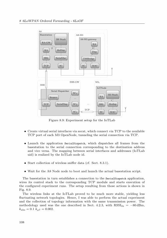
8 6LoWPAN Ordered Forwarding - 6LoOF
A8
SSH-GW
A8-M3
M31
A8-M3 gateway
Basestation
IoTNode
Serial Dispatcher
TSSBridge
SC MAC
Disp
RA
SC
SerialMac
6loDisp
BS Stack
RA-GW
RA
SRL
TCP
TCP
Bounce
SerialDisp SC2
SC1
...
SCn
SSH
SC
SRL
RA
MAC
6lodisp
M3 Stack
TCP
...
22
i
Figure 8.9: Experiment setup for the IoTLab
• Create virtual serial interfaces via socat, which connect via TCP to the availableTCP port of each M3 OpenNode, tunneling the serial connection via TCP.
• Launch the application SerialDispatch, which dispatches all frames from thebasestation to the serial connection corresponding to the destination addressand vice versa. The mapping between serial interfaces and addresses (IoTLabuid) is realized by the IoTLab node id.
• Start collection of wireless sniffer data (cf. Sect. 8.3.1).
• Wait for the A8 Node node to boot and launch the actual basestation script.
The basestation in turn establishes a connection to the SerialDispatch application,wires its control stack to the corresponding TCP module and starts execution ofthe configured experiment runs. The setup resulting from those actions is shown inFig. 8.9.
The wireless links at the IoTLab proved to be much more stable, yielding lessfluctuating network topologies. Hence, I was able to perform the actual experimentand the collection of topology information with the same transmission power. Themethodology used was the one described in Sect. 4.2.3, with RSSIth = −80 dBm,kabs = 0.1 kσ2 = 0.002.
108

8.3 Experiment setup
1m
Figure 8.10: Nodes selection at Grenoble site comprising the TB-IoT network; green:experiment nodes, blue: basestation and gateway node, red: sniffer nodes
0
A4839579
B268 A677 A478 2861
9183 9567 B877 9982 1162 A779 A283
8871 A183 A383 A079 9769 9177 9883
9082 9879 9072 B078 A569
B177 9168 A172 9071
B279 B482
9267 9167 A476
9472
B780
C268
Figure 8.11: Static routing topology of TB-IoT and RS-IoT networks
109
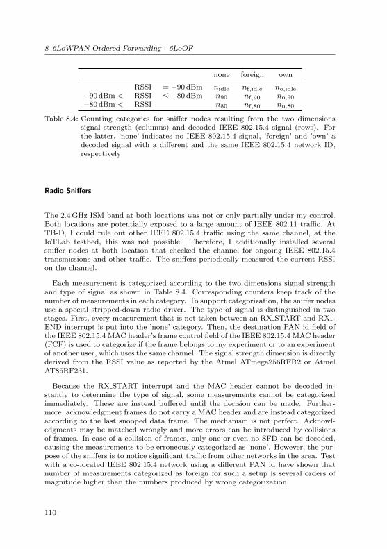
8 6LoWPAN Ordered Forwarding - 6LoOF
none foreign own
RSSI = −90 dBm nidle nf,idle no,idle
−90 dBm < RSSI ≤ −80 dBm n90 nf,90 no,90
−80 dBm < RSSI n80 nf,80 no,80
Table 8.4: Counting categories for sniffer nodes resulting from the two dimensionssignal strength (columns) and decoded IEEE 802.15.4 signal (rows). Forthe latter, ’none’ indicates no IEEE 802.15.4 signal, ’foreign’ and ’own’ adecoded signal with a different and the same IEEE 802.15.4 network ID,respectively
Radio Sniffers
The 2.4 GHz ISM band at both locations was not or only partially under my control.Both locations are potentially exposed to a large amount of IEEE 802.11 traffic. AtTB-D, I could rule out other IEEE 802.15.4 traffic using the same channel, at theIoTLab testbed, this was not possible. Therefore, I additionally installed severalsniffer nodes at both location that checked the channel for ongoing IEEE 802.15.4transmissions and other traffic. The sniffers periodically measured the current RSSIon the channel.
Each measurement is categorized according to the two dimensions signal strengthand type of signal as shown in Table 8.4. Corresponding counters keep track of thenumber of measurements in each category. To support categorization, the sniffer nodesuse a special stripped-down radio driver. The type of signal is distinguished in twostages. First, every measurement that is not taken between an RX START and RX -END interrupt is put into the ’none’ category. Then, the destination PAN id field ofthe IEEE 802.15.4 MAC header’s frame control field of the IEEE 802.15.4 MAC header(FCF) is used to categorize if the frame belongs to my experiment or to an experimentof another user, which uses the same channel. The signal strength dimension is directlyderived from the RSSI value as reported by the Atmel ATmega256RFR2 or AtmelAT86RF231.
Because the RX START interrupt and the MAC header cannot be decoded in-stantly to determine the type of signal, some measurements cannot be categorizedimmediately. These are instead buffered until the decision can be made. Further-more, acknowledgment frames do not carry a MAC header and are instead categorizedaccording to the last snooped data frame. The mechanism is not perfect. Acknowl-edgments may be matched wrongly and more errors can be introduced by collisionsof frames. In case of a collision of frames, only one or even no SFD can be decoded,causing the measurements to be erroneously categorized as ’none’. However, the pur-pose of the sniffers is to notice significant traffic from other networks in the area. Testwith a co-located IEEE 802.15.4 network using a different PAN id have shown thatnumber of measurements categorized as foreign for such a setup is several orders ofmagnitude higher than the numbers produced by wrong categorization.
110
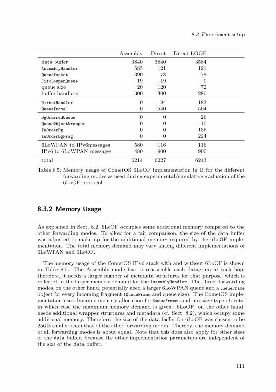
8.3 Experiment setup
Assembly Direct Direct-LOOF
data buffer 3840 3840 3584AssemblyHandler 585 121 121QueuePacket 390 78 78FifoLowpanQueue 19 19 0queue size 20 120 72buffer handlers 300 300 280
DirectHandler 0 184 183QueueFrame 0 540 504
DgOrderedQueue 0 0 26QueueObjectWrapper 0 0 10InOrderDg 0 0 135InOrderDgFrag 0 0 224
6LoWPAN to IPv6messages 580 116 116IPv6 to 6LoWPAN messages 480 900 900
total 6214 6227 6243
Table 8.5: Memory usage of CometOS 6LoOF implementation in B for the differentforwarding modes as used during experimental/simulative evaluation of the6LoOF protocol
8.3.2 Memory Usage
As explained in Sect. 8.2, 6LoOF occupies some additional memory compared to theother forwarding modes. To allow for a fair comparison, the size of the data bufferwas adjusted to make up for the additional memory required by the 6LoOF imple-mentation. The total memory demand may vary among different implementations of6LoWPAN and 6LoOF.
The memory usage of the CometOS IPv6 stack with and without 6LoOF is shownin Table 8.5. The Assembly mode has to reassemble each datagram at each hop,therefore, it needs a larger number of metadata structures for that purpose, which isreflected in the larger memory demand for the AssemblyHandler. The Direct forwardingmodes, on the other hand, potentially need a larger 6LoWPAN queue and a QueueFrame
object for every incoming fragment (QueueFrame and queue size). The CometOS imple-mentation uses dynamic memory allocation for QueueFrames and message type objects,in which case the maximum memory demand is given. 6LoOF, on the other hand,needs additional wrapper structures and metadata (cf. Sect. 8.2), which occupy someadditional memory. Therefore, the size of the data buffer for 6LoOF was chosen to be256 B smaller than that of the other forwarding modes. Thereby, the memory demandof all forwarding modes is about equal. Note that this does also apply for other sizesof the data buffer, because the other implementation parameters are independent ofthe size of the data buffer.
111
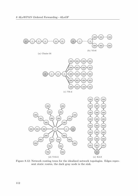
8 6LoWPAN Ordered Forwarding - 6LoOF
0 1 3 4 14 15
(a) Chain-16
0 1 5
100
200
101
202
105
205
(b) Y3-6
0 1 2 3
100 101 102 103
200 201 202 203
300 301 302 303
400 401 402 403
500 501 502 503
(c) Y6-4
012
100
101
102
200
201
202
300
301
302
400
401
402
500501502
600
601
602
700
701
702
800
801
802
900
901
902
(d) Y10-3
0
101
102
103
104
105
106
107
108
201
202
203
204
205
206
207
208
301
302
303
304
305
306
307
308
(e) X3-8
Figure 8.12: Network routing trees for the idealized network topologies. Edges repre-sent static routes, the dark gray node is the sink.
112
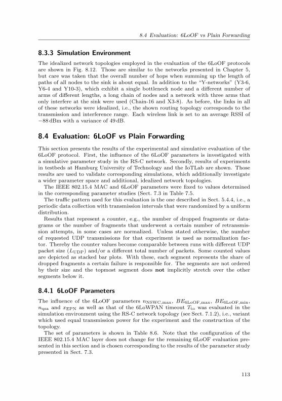
8.4 Evaluation: 6LoOF vs Plain Forwarding
8.3.3 Simulation Environment
The idealized network topologies employed in the evaluation of the 6LoOF protocolsare shown in Fig. 8.12. Those are similar to the networks presented in Chapter 5,but care was taken that the overall number of hops when summing up the length ofpaths of all nodes to the sink is about equal. In addition to the “Y-networks” (Y3-6,Y6-4 and Y10-3), which exhibit a single bottleneck node and a different number ofarms of different lengths, a long chain of nodes and a network with three arms thatonly interfere at the sink were used (Chain-16 and X3-8). As before, the links in allof these networks were idealized, i.e., the shown routing topology corresponds to thetransmission and interference range. Each wireless link is set to an average RSSI of−88 dBm with a variance of 49 dB.
8.4 Evaluation: 6LoOF vs Plain Forwarding
This section presents the results of the experimental and simulative evaluation of the6LoOF protocol. First, the influence of the 6LoOF parameters is investigated witha simulative parameter study in the RS-C network. Secondly, results of experimentsin testbeds at Hamburg University of Technology and the IoTLab are shown. Thoseresults are used to validate corresponding simulations, which additionally investigatea wider parameter space and additional, idealized network topologies.
The IEEE 802.15.4 MAC and 6LoOF parameters were fixed to values determinedin the corresponding parameter studies (Sect. 7.3 in Table 7.5.
The traffic pattern used for this evaluation is the one described in Sect. 5.4.4, i.e., aperiodic data collection with transmission intervals that were randomized by a uniformdistribution.
Results that represent a counter, e.g., the number of dropped fragments or data-grams or the number of fragments that underwent a certain number of retransmis-sion attempts, in some cases are normalized. Unless stated otherwise, the numberof requested UDP transmissions for that experiment is used as normalization fac-tor. Thereby the counter values become comparable between runs with different UDPpacket size (LUDP) and/or a different total number of packets. Some counted valuesare depicted as stacked bar plots. With these, each segment represents the share ofdropped fragments a certain failure is responsible for. The segments are not orderedby their size and the topmost segment does not implicitly stretch over the othersegments below it.
8.4.1 6LoOF Parameters
The influence of the 6LoOF parameters nNSWC,max, BE6LoOF,max, BE6LoOF,min,nqsa and xEPN as well as that of the 6LoWPAN timeout Tto was evaluated in thesimulation environment using the RS-C network topology (see Sect. 7.1.2), i.e., variantwhich used equal transmission power for the experiment and the construction of thetopology.
The set of parameters is shown in Table 8.6. Note that the configuration of theIEEE 802.15.4 MAC layer does not change for the remaining 6LoOF evaluation pre-sented in this section and is chosen corresponding to the results of the parameter studypresented in Sect. 7.3.
113
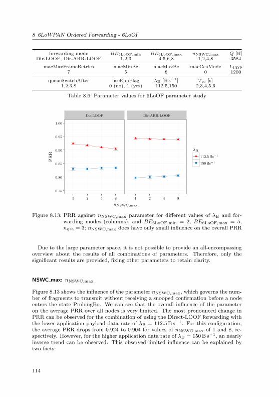
8 6LoWPAN Ordered Forwarding - 6LoOF
forwarding mode BE6LoOF,min BE6LoOF,max nNSWC,max Q [B]Dir-LOOF, Dir-ARR-LOOF 1,2,3 4,5,6,8 1,2,4,8 3584
macMaxFrameRetries macMinBe macMaxBe macCcaMode LUDP
7 5 8 0 1200
queueSwitchAfter useEpnFlag λB [B s−1] Tto [s]1,2,3,8 0 (no), 1 (yes) 112.5,150 2,3,4,5,6
Table 8.6: Parameter values for 6LoOF parameter study
Dir-LOOF Dir-ARR-LOOF
0.75
0.80
0.85
0.90
0.95
1.00
1 2 4 8 1 2 4 8
nNSWC,max
PR
R
λB
112.5Bs−1
150Bs−1
Figure 8.13: PRR against nNSWC,max parameter for different values of λB and for-warding modes (columns), and BE6LoOF,min = 2, BE6LoOF,max = 5,nqsa = 3; nNSWC,max does have only small influence on the overall PRR
Due to the large parameter space, it is not possible to provide an all-encompassingoverview about the results of all combinations of parameters. Therefore, only thesignificant results are provided, fixing other parameters to retain clarity.
NSWC max: nNSWC,max
Figure 8.13 shows the influence of the parameter nNSWC,max, which governs the num-ber of fragments to transmit without receiving a snooped confirmation before a nodeenters the state ProbingBo. We can see that the overall influence of the parameteron the average PRR over all nodes is very limited. The most pronounced change inPRR can be observed for the combination of using the Direct-LOOF forwarding withthe lower application payload data rate of λB = 112.5 B s−1. For this configuration,the average PRR drops from 0.924 to 0.904 for values of nNSWC,max of 1 and 8, re-spectively. However, for the higher application data rate of λB = 150 B s−1, an nearlyinverse trend can be observed. This observed limited influence can be explained bytwo facts:
114
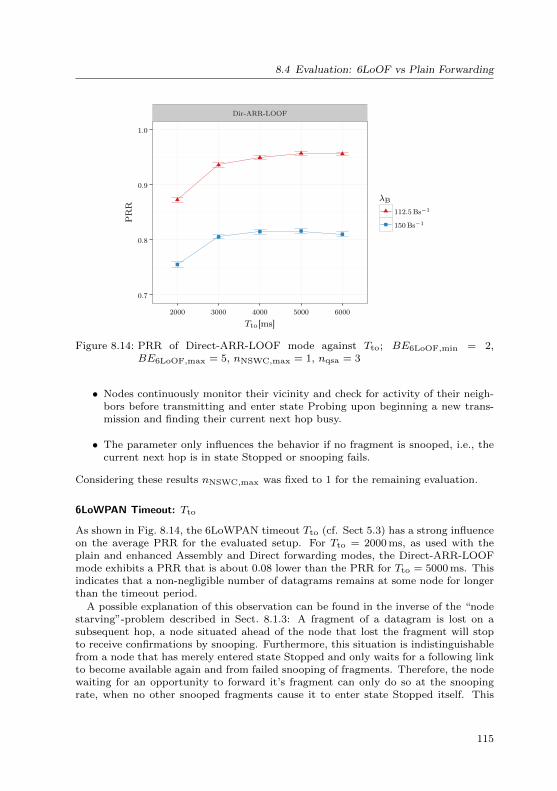
8.4 Evaluation: 6LoOF vs Plain Forwarding
Dir-ARR-LOOF
0.7
0.8
0.9
1.0
2000 3000 4000 5000 6000
Tto[ms]
PR
R
λB
112.5Bs−1
150Bs−1
Figure 8.14: PRR of Direct-ARR-LOOF mode against Tto; BE6LoOF,min = 2,BE6LoOF,max = 5, nNSWC,max = 1, nqsa = 3
• Nodes continuously monitor their vicinity and check for activity of their neigh-bors before transmitting and enter state Probing upon beginning a new trans-mission and finding their current next hop busy.
• The parameter only influences the behavior if no fragment is snooped, i.e., thecurrent next hop is in state Stopped or snooping fails.
Considering these results nNSWC,max was fixed to 1 for the remaining evaluation.
6LoWPAN Timeout: Tto
As shown in Fig. 8.14, the 6LoWPAN timeout Tto (cf. Sect 5.3) has a strong influenceon the average PRR for the evaluated setup. For Tto = 2000 ms, as used with theplain and enhanced Assembly and Direct forwarding modes, the Direct-ARR-LOOFmode exhibits a PRR that is about 0.08 lower than the PRR for Tto = 5000 ms. Thisindicates that a non-negligible number of datagrams remains at some node for longerthan the timeout period.
A possible explanation of this observation can be found in the inverse of the “nodestarving”-problem described in Sect. 8.1.3: A fragment of a datagram is lost on asubsequent hop, a node situated ahead of the node that lost the fragment will stopto receive confirmations by snooping. Furthermore, this situation is indistinguishablefrom a node that has merely entered state Stopped and only waits for a following linkto become available again and from failed snooping of fragments. Therefore, the nodewaiting for an opportunity to forward it’s fragment can only do so at the snoopingrate, when no other snooped fragments cause it to enter state Stopped itself. This
115

8 6LoWPAN Ordered Forwarding - 6LoOF
1 2 3
0.75
0.80
0.85
0.90
0.95
1.00
4 5 6 8 4 5 6 8 4 5 6 8
BE6LoOF,max
PR
R
λB
112.5Bs−1
150Bs−1
Figure 8.15: PRR of Direct-ARR-LOOF mode against BE6LoOF,max for differentvalue of λB and BE6LoOF,min (columns); nqsa = 3, nNSWC,max = 1.
issue is also suspected to be one of the major problems of the 6LoOF mechanism inits form as presented in this thesis.
Minimum and Maximum Probing Exponents: BE6LoOF,min, BE6LoOF,max
Examination of the backoff exponents of the 6LoOF probing timer also revealed alimited influence for the given network. The results for Direct-ARR-LOOF with abuffer of Q = 3584 B and nqsa = 3 are shown in Figure 8.15, which governs whenthe 6LoOF protocol pushes a datagram to the end of its transmission queue afterthis datagram was not able to provide new fragments (cf. Sect. 8.1.3). The PRRis lower for the larger examined values of BE6LoOF,max, independently from λB andBE6LoOF,min. The overall difference between BE6LoOF,max = 4 and BE6LoOF,max =8 is less than 0.025. The overall influence of the BE6LoOF,min parameter on thePRR even less pronounced. For the higher of the two data rates λB = 150 B s−1,the PRR curve is shifted to lower values for BE6LoOF,min = 3. For the lower datarate of λB = 112.5 B s−1, BE6LoOF,min = 2 exhibits the highest PRR. Similar to thenNSWC,max parameter, the influence on the PRR is limited. BE6LoOF,min = 2 andBE6LoOF,max = 4 were chosen as parameters for further evaluation.
Push Back Stale Datagrams: nqsa
Similar observations can be made for the nqsa parameter (Fig. 8.16). For the higherof the examined data rates λB = 150 B s−1, the highest PRR is achieved for nqsa = 1,the lowest for nqsa = 8. With λB = 112.5 B s−1, in contrast, the lowest PRR isobserved for nqsa = 1. nqsa = 3 was chosen as a compromise.
116

8.4 Evaluation: 6LoOF vs Plain Forwarding
3584B
0.75
0.80
0.85
0.90
0.95
1.00
1 2 3 8
nqsa
PR
R
λB
112.5Bs−1
150Bs−1
Figure 8.16: PRR of Direct-ARR-LOOF mode against nqsa for two different values ofλB; BE6LoOF,min = 2, BE6LoOF,max = 4
112.5Bs−1 150Bs−1
0.75
0.80
0.85
0.90
0.95
1.00
4 5 6 8 4 5 6 8
BE6LoOF,max
PR
R
xEPN
0
1
Figure 8.17: PRR of Direct-ARR-LOOF mode against BE6LoOF,max with xEPN setand cleared for varying λB; BE6LoOF,min = 2
117

8 6LoWPAN Ordered Forwarding - 6LoOF
BE6LoOF,min BE6LoOF,max nqsa nNSWC,max Tto (ms)
2 4 3 1 5000
Table 8.7: 6LoOF parameters used for evaluation
Q [B] LUDP [B]
3840 (3584) 1200
Table 8.8: Traffic generator parameters for 6LoOF evaluation in testbed
useEpnFlag: xEPN
Figure 8.17 shows the impact of explicit probing notification. As can be seen, itis rather limited. Only for BE6LoOF,max = 8 the PRR without using the flaggingmechanism (cf. Sect. 8.1.2) is more than 0.01 lower than the corresponding PRRusing the mechanism. For the other observations the PRR is lower by less than0.01. These findings support the hypothesis that flagging outgoing fragments doesnot greatly improve the performance of 6LoOF in terms of reliability. In the lightof those results, not using the flagging mechanism is clearly preferred, especially asit allows an implementation of 6LoOF without alteration to the 6LoWPAN fragmentheader format.
6LoOF Parameters: Summary
This section examined the influence of the parameters defined for the 6LoOF protocolon the average PRR for the examined traffic scenario and forwarding modes. Onereason for the limited impact is that they change the behavior of 6LoOF mainly insituations that represent an error case. For example, the nqsa parameter influences thehandling of the 6LoWPAN transmission queue only if subsequent fragments belongingto the active datagram are missing. Apart from nodes that encounter a stopped nodeas their next hop, probing is used only when snooping fails.
The 6LoOF parameters are fixed for the comparative evaluation of 6LoOF with theother forwarding modes to the values shown in Table 8.7.
8.4.2 TB-IoT Experiments
Due to the contention for the nodes in the IoTLab with other researchers and a com-paratively large number of runs to get sound results for both testbed experiments, theconfiguration of the traffic generator was restricted to the values shown in Table 8.8.xEPN was varied for both testbeds. The transmission rate of UDP packets λB wasconstant within each testbed but adapted to the examined network topology.
During the experiment at the Grenoble site of the IoTLab, nodes used the sametransmission power that was used to determine the network topology (cf. Sect. 8.3.1).λB was set in a way to produce a total network traffic (considering all paths of allnodes as in (7.2)) of λB,total = 6600 B. This configuration is shown in Tbl. 8.9.
118

8.4 Evaluation: 6LoOF vs Plain Forwarding
λB[B s−1] P tx [dBm] xEPN
37.5 -2.5 0,1
Table 8.9: Parameter setting for TB-IoT experiment
RS-IoT TB-IoT
0.75
0.80
0.85
0.90
0.95
1.00
1200 1200
LUDP [B]
PR
R
ModeAss
Dir
Dir-ARR
Dir-LOOF
Dir-ARR-LOOF
Figure 8.18: PRR of TB-IoT testbed and derived simulation scenario; xEPN = 1
PRR in Comparison to Simulation
Figure 8.18 shows the PRR obtained in the IoTLab and a corresponding simulationscenario derived using the method described in Sect. 4.3. The results show that forthe given configuration, the 6LoOF mechanism achieves the best performance of allforwarding modes in terms of PRR, in simulation and testbed. With a PRR of 0.982the PRR obtained by the Direct-ARR-LOOF mode is larger by 0.037 than that ofthe Assembly mode (0.945) and by 0.026 than that of the Direct-ARR (0.956). Tothe plain Direct mode, the gap is significantly larger. Note that while the differenceseems small it can be also translated to losing less than half as many datagrams thanthe next-best forwarding mode. The Direct-LOOF mode, with exception of the plainDirect mode, achieves a lower PRR than the other modes.
Comparing the results from the testbed with the corresponding simulation, the mostnotable difference is the better PRR exhibited by Direct and Direct-LOOF modes. TheDirect-LOOF forwarding achieves a PRR slightly higher than that of the Assemblymode and also outperforms the Direct-ARR mode. The Direct mode achieves a PRRthat is 0.14 higher than the one observed in the testbed. In general, the other modesperform slightly better in the simulation environment. While Direct-ARR-LOOF stillis the mode with the highest PRR, the margin is less pronounced in the simulationenvironment.
The influence of the xEPN parameter is shown in Fig. 8.19. The results support thestatement in Sect. 8.4.1 – xEPN = 1 does not have a significant positive influence onthe average PRR and therefore the flagging mechanism can be deactivated.
119

8 6LoWPAN Ordered Forwarding - 6LoOF
0 1
0.75
0.80
0.85
0.90
0.95
1.00
TB
-IoT
1200 1200
LUDP [B]
PR
R
ModeAss
Dir
Dir-ARR
Dir-LOOF
Dir-ARR-LOOF
Figure 8.19: PRR of IoTLab testbed for xEPN ∈ [0, 1] (columns)
Drop Causes
Looking at the causes for dropped fragments (Fig. 8.20), we can observe that the byfar dominating cause for lost fragments are transmission failures at the link layer.Further investigation reveals that among the causes for these drops a consecutivelyfailed CCA and in consequence a failed CSMA/CA is the dominant one. This istrue for both simulation and testbed environment and corresponds to the findings inSect. 7.3.3. The notable differences in simulation and testbed environment for thedifferent forwarding modes can be directly translated to the observations made forthe PRR.
Sniffing
In general, the experiments at the Grenoble site of the IoTLab have been executedat night in a rather quite environment with regard to interference by other wirelesstechnologies. The installed sniffers record a basic noise, which is supposed to be causedby idle beaconing of IEEE 802.11 access points and misinterpretation of transmissionbelonging to the experiment network itself (cf. Sect. 8.3.1). This “background noise”shows no significant correlation with the results of the experiment. However, with oneset of experiments, a more significant interference was recorded.
Figure 8.21 shows a normalized number of registered non-idle sniffer measurementsplotted against real-time together with a scatter plot of the average PRR obtained forthe Assembly mode. It can be seen that during one of last sets of experiments, the PRRdecreases significantly while at the same time the number of non-idle measurementsincreases significantly. Similar results can be observed for the other forwarding modes(except Direct-ARR-LOOF, whose runs in that period were invalid and removed due tonodes crashing during that particular set of experiments) during the execution of thisset of experiments. This result also explains the slightly higher confidence intervalsobservable in Fig. 8.19, which shows the results of the experiment with significant
120

8.4 Evaluation: 6LoOF vs Plain Forwarding
RS-IoT TB-IoT
0.00
0.05
0.10
0.15
0.20Ass
Dir
Dir-A
RR
Dir-LOOF
Dir-A
RR-LOOF
Ass
Dir
Dir-A
RR
Dir-LOOF
Dir-A
RR-LOOF
Mode
#da
tagram
s(norm)
dropReasonMacFail
BufferFull
(a) Drop causes
RS-IoT TB-IoT
0
2
4
6
Ass
Dir
Dir
-AR
R
Dir
-LO
OF
Dir
-AR
R-L
OO
F
Ass
Dir
Dir
-AR
R
Dir
-LO
OF
Dir
-AR
R-L
OO
F
Mode
#fr
ames
(nor
m) retries
#retries6
#retries7
#CCA_fail
#fail
(b) IEEE 802.15.4 MAC drop causes
Figure 8.20: Drop causes for fragments of IoTLab testbed and derived simulation sce-nario
121

8 6LoWPAN Ordered Forwarding - 6LoOF
Ass
0.00
0.25
0.50
0.75
1.00
MÃďr 28 Apr 04 Apr 11 Apr 18 Apr 25
time
PRR
Sniffer208
251
287
Figure 8.21: Working of the radio sniffer during IoTLab experiment. Scatter plotshowing the PRR along with the normalized step plot of the number ofsniffer measurements registering unrecognizable signals with an energy inthe interval [−80,−90] dBm: n90 × 10. Results are shown for all threesniffer nodes (see Fig. 8.10)
sniffer activity. This shows that the installed radio sniffers are viable to detect periodsof increased interference by other networks.
Summary
There are several possible approaches to explain significantly better performance of thenon-delayed Direct modes in the simulation environment, as observed in Sect. 8.4.2.First, the simulation model may underestimate the busyness on the wireless channel,i.e., the CCA fails more often in the real testbed due an energy detection yielding aresult that is larger than the macCcaTh of −90 dBm. However, the data obtainedfrom the radio sniffers show a ratio of busy to total measurements of below 1 % mostof the time and therefore rule out this possibility.
Secondly, it is possible that the simulation underestimates the capability of thetransceiver to successfully decode the IEEE 802.15.4 SFD of an incoming frame evenif the signal is weak. Recall that the used transceiver tries to completely receive a framebefore it is ready to receive another one and the used macCcaMode reports a channelas busy if a frame is currently being decoded. Therefore, an increased capability tosuccessfully decode the SFD of weak signals can worsen the overall performance ofthe testbed. During topology construction, all received frames with a received signalstrength of −90 dBm were put into a bin representing RSSI values in the interval[−90,−100] dBm. A link that primarily produces measurements of this uncertaintype results in a simulated link with an average RSSI in the interval [−90,−100] dBm.As shown in Fig. 4.3, the simulation model will successfully decode an SFD with aprobability near 1, which does not provide much room for underestimation. However,during construction of the topology, only frames received successfully, i.e., with a
122

8.4 Evaluation: 6LoOF vs Plain Forwarding
λB [B s−1] P tx [dBm] xEPN
112.5 -3.5 0,1
Table 8.10: Parameter setting for TB-D experiment
TB-D
0.75
0.80
0.85
0.90
0.95
1.00
0 1
xEPN
PR
R
ModeAss
Dir
Dir-ARR
Dir-LOOF
Dir-ARR-LOOF
Figure 8.22: PRR in TB-D against xEPN
correct CRC are actually passed to the TopologyMonitor. Frames with a successfullydecoded SFD but a failed CRC check are discarded and are not counted. This meansthat some “SFD-capable” links may exist in the testbed that are not recorded in thecorresponding simulation environment and thereby produce the described effect.
8.4.3 TB-D Experiments
Due to the observed fluctuation of link qualities, the experiment in the testbed atHamburg University of Technology used a slightly increased transmission power P tx
compared to the transmission power used to determine the routing topology. Thetransmission rate of UDP packets in the traffic generator was set to generate a totaltraffic rate of λB,total = 4387.5 B s−1.
PRR and xEPN
At a first glance, the results from the TB-D contrast those obtained from the IoTLaband simulations.
Figure 8.22 suggests that without using the flagging mechanism (cf. Sect. 8.1.2), theaverage PRR achieved by the Direct-ARR-LOOF forwarding mode drops by 0.1, alongwith similarly strong pronounced drops of all other modes. The comparatively largeconfidence interval also hint at a strong fluctuation in the results for individual runs.
123

8 6LoWPAN Ordered Forwarding - 6LoOF
It has to be noted that while the experiments for the non-6LoOF forwarding modeswere repeated along with those for the 6LoOF modes, the value of xEPN does nothave any influence on the behavior of those modes. Therefore, the xEPN parametercan not be the sole source of influence in this case.
Drop Causes
Examining the number of fragments dropped and the corresponding causes (Fig. 8.23a),it becomes evident that a major part of dropped fragments was caused by the nodewith id 101. Furthermore, different from earlier observations, a dominant reason fora dropped fragment at the link-layer were consecutively failing retransmissions (andnot CSMA/CA failures; Fig. 8.23b). Note that while the execution of the differentmodes and their repeated runs were interleaved to counter temporarily varying links,the experiments sets for xEPN = 1 and xEPN = 0 had a gap of about two weeksbetween them. Therefore, an explanation in the observed behavior is, that the linkbetween nodes 101 and 105 was temporarily not available during the experiment withxEPN = 0.
This explanation is further supported by the scatter plot of the PRR averaged overall nodes (Fig. 8.24). There is a strikingly large number of measurements around aPRR of about 0.62 for all forwarding modes. With node 101 being the forwardingrouter for a part of the network containing 5 out of 13 nodes (8/13 ≈ 0.615), it is indeedplausible that during the runs achieving a PRR of about 0.62 the link was completelybroken. This assumption is further supported by the fact that the recordings of theradio sniffer located at the gateway node show no meaningful correlation with theobserved PRR values.
Apart from that, the scatter plots shows that there is a comparatively large variancebetween individual runs in general for the experiment set with xEPN = 0. This showsthat in this case, the measures taken to prevent the static routing topology fromworking did not prevent all problems and that the temporal variation of link qualityhas a large if not dominant influence on the results. Therefore, the obtained resultsare of limited usefulness.
However, the scatter plot also shows that the Direct-ARR-LOOF forwarding modestill exhibits a number of runs with a PRR near 1, which no other mode achieves.This indicates that the Direct-ARR-LOOF mode can outperform the other forwardingmodes in the given configuration if all links are present and healthy.
To compensate for the “broken link” effect, the measured data from the testbedwas adjusted by removing all runs that exhibited 100 or more fragments at any singlenode that underwent the maximum number of 7 IEEE 802.15.4 MAC retransmissions.
In consequence, the PRR of all forwarding modes is improved for both settingsof xEPN. While with xEPN = 0 the PRR on average is still lower compared toxEPN = 1, the relative performance among the forwarding modes is, with the exceptionof Direct-LOOF and Assembly, much more similar after the removal of the bad runs.
Comparison to Simluation
The comparison of simulation and adjusted testbed data (Fig. 8.25a) leads to resultssimilar to those obtained for the testbed in the IoTLab. The PRR obtained in simula-tion better by 0.03 (Direct-ARR, Direct-ARR-LOOF) to 0.17 (Direct-LOOF). Again,
124

8.4 Evaluation: 6LoOF vs Plain Forwarding
TB-D
0.0
0.4
0.8
1.2
0.0
0.4
0.8
1.2
0.0
0.4
0.8
1.2
Ass
Dir-A
RR
Dir-A
RR-LOOF
105
101
106
107
102
103
104
108
109
10A
10B
10C
100
avg
Node Id and avg
#da
tagram
s(norm)
dropReasonMacFail
BufferFull
(a) Drop causes
0
1
2
3
0
1
2
3
01
Ass Dir Dir-ARR Dir-LOOFDir-ARR-LOOF
Mode
#fr
ames
(nor
m) retries
#retries6
#retries7
#CCA_fail
#fail
(b) IEEE 802.15.4 MAC drop causes
Figure 8.23: Drop causes for fragments of TB-D testbed and derived simulation sce-nario. Rows represent forwarding mode (8.23a) and xEPN (8.23b)
125

8 6LoWPAN Ordered Forwarding - 6LoOF
Ass Dir Dir-ARR Dir-LOOF Dir-ARR-LOOF
0.6
0.7
0.8
0.9
1.0
TB
-D
0 50 100 150 200 0 50 100 150 200 0 50 100 150 200 0 50 100 150 200 0 50 100 150 200
run number
PR
R
Figure 8.24: Scatter plot of the PRR averaged over all nodes for individual runs fordifferent forwarding modes (columns); xEPN=0
the non-delayed forwarding modes Direct and Direct-LOOF achieve a better PRR inthe simulation environment than in the testbed. For the TB-D, however, the mainreason for the simulation environment to exhibit a better PRR is the larger number offrames dropped due to consecutively failed retransmissions in the testbed even afterthe adjustment and not a larger number of CCA failures as can be seen in Fig. 8.25b.
8.4.4 Simulation
The simulation runs iterate over λB, Q and LUDP. Some of the networks introducedin Sect. 8.3.3 differ with respect to the total number of hops that have to be traversedfor the traffic of all nodes to reach its destination. Therefore, the total traffic rateλB,total would vary significantly if λB was equal for all networks. To enable a roughcomparison between the different topologies, λB is set to reflect four categories oftraffic load T: Tlow, Tmid, Thigh and Tmax.
Table 8.11 shows the setting for each network and the corresponding resultingλB,total and traffic category. 6LoWPAN buffer space is classified into three cate-gories QS, QM and QL, corresponding to Q ∈ {2560, 3840, 5120}B for non-6LoOFand to Q ∈ {2304, 3584, 4846}B for 6LoOF forwarding modes. Furthermore, all sim-ulation runs were carried out for different values of the UDP packet size LUDP ∈{400, 800, 1200}B.
126

8.4 Evaluation: 6LoOF vs Plain Forwarding
RS-D1 TB-D TB-Df
0.75
0.80
0.85
0.90
0.95
1.00
1 1 1
xEPN
PR
R
ModeAss
Dir
Dir-ARR
Dir-LOOF
Dir-ARR-LOOF
(a) PRR
0.0
0.5
1.0
1.5
2.0
0.0
0.5
1.0
1.5
2.0
0.0
0.5
1.0
1.5
2.0
RS-D
1T
B-D
TB
-Df
Ass Dir Dir-ARR Dir-LOOFDir-ARR-LOOF
Mode
#fr
ames
(nor
m) retries
#retries6
#retries7
#CCA_fail
#fail
(b) IEEE 802.15.4 MAC drop causes
Figure 8.25: PRR and MAC drop causes for TB-D, adjusted TB-Df and derived sim-ulation network
127
8 6LoWPAN Ordered Forwarding - 6LoOF
Networks htotal Tlow Tmid Thigh Tmax
RS-C1 57 75.0|4275.0|16 112.5|6412.5|11 150.0|8550.0|8.0 234.4|13360|5.1RS-D1, RS-D2 39 112.5|4385.5|11 150.0|5850.0|8 187.5|7312.5|6.4 337.5|13163|3.6
RS-IoT 176 28.1|4950.0|43 37.5|6600.0|32 56.3|9900.0|21 75.0|13200|16
Chain-16 120 37.5|4500.0|32 56.3|6750.0|21 75.0|9000.0|16 112.5|13500|11Y3-6 117 37.5|4387.5|32 56.3|6581.3|21 75.0|8775.0|16 112.5|13163|11Y6-4 116 37.5|4350.0|32 56.3|6525.0|21 75.0|8700.0|16 112.5|13050|11Y10-3 111 37.5|4162.5|32 56.3|6243.8|21 75.0|8325.0|16 112.5|12488|11X3-8 108 37.5|4050.0|32 56.3|6075.0|21 75.0|8100.0|16 112.5|12150|11
Table 8.11: 6LoOF simulation runs; λB[B s−1]|λB,total[B s−1]|i[s] for different trafficload categories
Overview of PRR Performance
First, mind that the scale of the y-axis does not begin at zero to better visualizesmaller differences. To get an accurate impression, the PRR bar plots have to beregarded as a zoomed-in and cut-off top section of the PRR. Note also that for theT = Tmax of the testbed-derived networks only the RS-IoT network maintains a PRRabove 0.6. The other two networks enter a congested state for that transmission rate
QS QM QL
0.7
0.8
0.9
1.0
0.7
0.8
0.9
1.0
0.7
0.8
0.9
1.0
RS-C
1R
S-IoTR
S-D2
Tlow TmidThighTmax Tlow TmidThighTmax Tlow TmidThighTmax
T
PR
R
ModeAss
Dir
Dir-ARR
Dir-LOOF
Dir-ARR-LOOF
Figure 8.26: PRR against traffic load T for testbed-derived networks (rows), differentbuffer sizes (columns) and forwarding modes (bar color). The payloadwas set to LUDP = 1200 B
128

8.4 Evaluation: 6LoOF vs Plain Forwarding
QS QM QL
0.50.60.70.80.91.0
0.50.60.70.80.91.0
0.50.60.70.80.91.0
0.50.60.70.80.91.0
0.50.60.70.80.91.0
Chain-16
X3-8
Y3-6
Y10-3
Y6-4
Tlow TmidThighTmax Tlow TmidThighTmax Tlow TmidThighTmax
T
PR
R
ModeAss
Dir
Dir-ARR
Dir-LOOF
Dir-ARR-LOOF
Figure 8.27: PRR against traffic load T for idealized networks (rows), different buffersizes (cols) and forwarding modes (bar color). The UDP packet payloadwas set to LUDP = 1200 B
and the PRR drops as low as 0.4 for those networks and is deliberately cut off inFig. 8.26 to retain visibility of differences for the other rates.
Figure 8.26 shows the average PRR for all testbed-derived networks and a UDPpayload LUDP = 1200 B. For the smallest of the evaluated 6LoWPAN buffer sizes,the 6LoOF mechanism significantly improves the PRR for all networks and all rates incomparison to the Direct-ARR mode, which consistently achieves the best performanceof non-6LoOF forwarding modes. With increasing Q, the PRR of the Assembly modesignificantly increases, causing it to obtain the best result of the non-6LoOF modes.However, the performance of Direct-ARR-LOOF is still better for all evaluated trafficloads in networks RS-IoT and RS-D1. An exception can be identified with the RS-C1 network, in which the Assembly mode achieves the highest PRR for T = Thigh
and 6LoWPAN buffer size QL. Another observation is, that in this network, theDirect-LOOF mode achieves a higher PRR than Direct-ARR-LOOF for T = Thigh.
It can also be observed that the PRR of the 6LoOF modes is not significantlyincreased by switching from a QM to a QL buffer. This is similar to the Direct modes.However, even for the QS buffer, 6LoOF outperforms the plain Direct forwardingmodes by 0.03 to 0.07. The gap to the Assembly mode is significantly larger for aQS buffer, especially for T = Thigh, e.g., 0.1 in network RS-IoT and 0.15 in networkRS-D2. This indicates that the goal for 6LoOF to work with restricted buffer spaceis fulfilled.
129

8 6LoWPAN Ordered Forwarding - 6LoOF
The observations for the idealized networks are mainly consistent with those forthe testbed-derived ones (Fig. 8.27). Interestingly, while the λB,total is similar to thetestbed-derived networks and among the idealized ones, there are significant differ-ences with regard to the PRR-performance. In Chain-16, Y3-6 and X3-8 networks,the PRR achieved by 6LoOF up to T = Thigh is near 1. This can be attributed to thesharply cut interference range that reaches only the direct neighbor of each node in theidealized topologies. Thereby, contention on the wireless channel is greatly reducedcompared to the testbed-derived networks. 6LoOF can be identified as the forwardingmode achieving the best results. Especially in the Y10-3 and Y6-4 networks, 6LoOFexhibits a better PRR for T = Thigh, with the non-rate-restricted Direct-LOOF modeperforming better that the rate-restricted Direct-ARR-LOOF. The latter fact is plau-sible considering the topology of Y10-3 and the limited potential for pipelining frag-ments in that network.
It has to be noted that approaching congestion in networks Y10-3 and Y6-4 withT = Tmax, the performance of both 6LoOF modes and that of the Direct-ARR modedecrease in comparison to the other forwarding modes. This behavior indicates that6LoOF is not as well suited in an already congested network. Section 8.1.3 shortlydiscussed a possible explanation for this behavior: If a successor node has to dropa datagram, a predecessor node will always transmit with snooping rate towards itbecause it will never get a confirmation for its fragments.
The results of the comparison between the real testbed and derived simulation envi-ronments in Sect. 8.4.2 and Sect. 8.4.3 show a significantly higher PRR in simulationespecially for the non-rate-restricted Direct modes. This has to be kept in mind whenassessing the simulation results.
Drop Causes
Exemplarily, the causes for dropped fragments are investigated for a 6LoWPAN bufferof size Q ∈ {QS,QL}, T = Thigh and UDP packet size LUDP = 1200 B in RS-IoT andY10-3 networks.
Examining the general causes for dropping fragments (Fig 8.28a) in the RS-IoTnetwork, it becomes evident that a lack of buffer space and failures at the link-layer arethe only causes for failures. For the larger 6LoWPAN buffer size, the number of dropsdue to link-layer transmission failures is increased. This can be explained by a strongercontention for the wireless channel due to less fragments being rejected because ofmissing buffer space. For the Assembly mode, which has the largest reduction ofbuffer drops with the larger buffer size, the number of link-layer failures increasesmore significantly.
Furthermore, it can be observed that the 6LoOF mechanism effectively reducesboth buffer drops and transmission failures. While Direct-LOOF exhibits less bufferdrops than Direct-ARR-LOOF, this is more than compensated for by the significantlyreduced number of transmission failures.
In RS-IoT, the dominant specific reason for transmission failures can again be iden-tified as CSMA/CA failures (Fig. 8.28b). 6LoOF is not only able to reduce the numberof failures caused by consecutively failed retransmissions to near zero, but also exhibitsa much smaller number of CSMA/CA failures, i.e., consecutively failed CCAs.
The results are quite different for the idealized Y10-3 network, which containsshorter paths and a single bottleneck at node 2 (Fig. 8.12d). Here, even for the large
130

8.4 Evaluation: 6LoOF vs Plain Forwarding
QS QL
0.0
0.1
0.2
0.0
0.1
0.2
RS-IoT
Y10-3
Ass
Dir
Dir-A
RR
Dir-LOOF
Dir-A
RR-LOOF
Ass
Dir
Dir-A
RR
Dir-LOOF
Dir-A
RR-LOOF
Mode
#da
tagram
s(norm)
dropReasonQueueFull
MacFail
BufferFull
OutOfHandlers
AssemblyFull
TinyFull
OutOfMessages
(a) General drop causes
QS QL
0.00
0.05
0.10
0.00
0.05
0.10
RS-IoT
Y10-3
Ass
Dir
Dir
-AR
R
Dir
-LO
OF
Dir
-AR
R-L
OO
F
Ass
Dir
Dir
-AR
R
Dir
-LO
OF
Dir
-AR
R-L
OO
F
Mode
#fr
ames
(nor
m) retries
#retries6
#retries7
#CCA_fail
#fail
(b) IEEE 802.15.4 MAC drop causes
Figure 8.28: Causes for dropping of fragments in general and at the IEEE 802.15.4link-layer in detail in RS-IoT and Y10-3 networks for LUDP = 1200 B
131
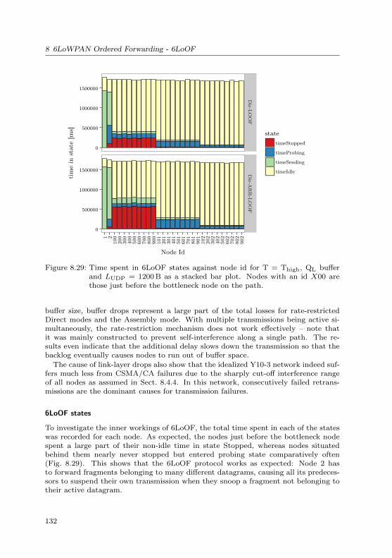
8 6LoWPAN Ordered Forwarding - 6LoOF
0
500000
1000000
1500000
0
500000
1000000
1500000
Dir-L
OO
FD
ir-AR
R-L
OO
F
1 210
020
030
040
050
060
070
080
090
010
120
130
140
150
160
170
180
190
110
220
230
240
250
260
270
280
290
2
Node Id
tim
ein
stat
e[m
s] statetimeStopped
timeProbing
timeSending
timeIdle
Figure 8.29: Time spent in 6LoOF states against node id for T = Thigh, QL bufferand LUDP = 1200 B as a stacked bar plot. Nodes with an id X00 arethose just before the bottleneck node on the path.
buffer size, buffer drops represent a large part of the total losses for rate-restrictedDirect modes and the Assembly mode. With multiple transmissions being active si-multaneously, the rate-restriction mechanism does not work effectively – note thatit was mainly constructed to prevent self-interference along a single path. The re-sults even indicate that the additional delay slows down the transmission so that thebacklog eventually causes nodes to run out of buffer space.
The cause of link-layer drops also show that the idealized Y10-3 network indeed suf-fers much less from CSMA/CA failures due to the sharply cut-off interference rangeof all nodes as assumed in Sect. 8.4.4. In this network, consecutively failed retrans-missions are the dominant causes for transmission failures.
6LoOF states
To investigate the inner workings of 6LoOF, the total time spent in each of the stateswas recorded for each node. As expected, the nodes just before the bottleneck nodespent a large part of their non-idle time in state Stopped, whereas nodes situatedbehind them nearly never stopped but entered probing state comparatively often(Fig. 8.29). This shows that the 6LoOF protocol works as expected: Node 2 hasto forward fragments belonging to many different datagrams, causing all its predeces-sors to suspend their own transmission when they snoop a fragment not belonging totheir active datagram.
132
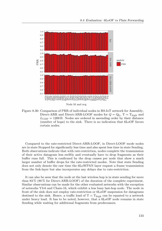
8.4 Evaluation: 6LoOF vs Plain Forwarding
0.5
0.6
0.7
0.8
0.9
1.0
0.5
0.6
0.7
0.8
0.9
1.0
0.5
0.6
0.7
0.8
0.9
1.0
Ass
Dir-A
RR
Dir-A
RR
-LO
OF
9579
A48
328
61A
478
A67
7B
268
1162
9183
9567
9982
A28
3A
779
B87
788
7191
7797
6998
83A
079
A18
3A
383
9072
9082
9879
A56
9B
078
9071
9168
A17
2B
177
B27
9B
482
9167
9267
A47
694
72B
780
C26
8av
gNode Id and avg
PR
R metricPRR
Figure 8.30: Comparison of PRR of individual nodes in RS-IoT network for Assembly,Direct-ARR and Direct-ARR-LOOF modes for Q = QL, T = Thigh andLUDP = 1200 B. Nodes are ordered in ascending order by their distance(number of hops) to the sink. There is no indication that 6LoOF favorscertain nodes.
Compared to the rate-restricted Direct-ARR-LOOF, in Direct-LOOF mode nodesare in state Stopped for significantly less time and also spent less time in state Sending.Both observations indicate that with rate-restriction, nodes complete the transmissionof their active datagram less swiftly and eventually have to drop fragments as theirbuffer runs full. This is confirmed by the drop causes per node that show a muchlarger number of buffer drops for the rate-restricted modes. Note that state Sendingdoes not only denote the raw time the 6LoWPAN layer request a frame transmissionfrom the link-layer but also incorporates any delays due to rate-restriction.
It can also be seen that the node at the last wireless hop is in state sending for morethan 83 % (88 % for Direct-ARR-LOOF) of the duration of the complete experiment.Similar observations can be made for the other evaluated networks with the exceptionof networks Y3-6 and Chain-16, which exhibit a less busy last-hop node. The node infront of the sink does not employ rate-restriction or 6LoOF suspension for datagramsdestined to the sink. Hence, a traffic load of T = Thigh can be equated to a networkunder heavy load. It has to be noted, however, that a 6LoOF node remains in stateSending while waiting for additional fragments from predecessors.
133

8 6LoWPAN Ordered Forwarding - 6LoOF
Fairness
Figure 8.30 shows the PRR for all nodes in the RS-IoT testbed for the forwardingmodes Assembly, Direct-ARR and Direct-ARR-LOOF and T = Thigh and LUDP =1200 B. Nodes are ordered in ascending order by their distance (number of hops) tothe sink. This figure is qualitatively representative for the other evaluated networks. Itshows that there is no significant preference to certain nodes by the 6LoOF protocol.While some differences in PRR between individual nodes exist, the pattern is verysimilar for all the shown forwarding modes and can not be attributed to the 6LoOFprotocol. That on average the PRR is slightly decreasing with the distance from thesink is to be expected, considering the increased potential for failures along longerpath (cf. Fig. 3.3) and can also not be attributed to the protocol itself. Comparedto the plain Direct-ARR forwarding, the absolute differences between nodes are evenless pronounced with 6LoOF.
UDPPacket size LUDP
For the QL 6LoWPAN buffer and T = Thigh the performance of the forwardingmodes for different UDP packet sizes is evaluated, while keeping the total data rateconstant. This is realized by adapting the average interval between packets accordingto λ = λB/LUDP. Note that the PRR is not directly comparable for the differentcombinations of λB and LUDP, because only individual packets are accounted for. Onthe one hand, the overhead caused by the UDP and IPv6 headers is larger for smallerpackets. On the other hand, losing one fragment per 1200 B payload for LUDP = 400 Btranslates into the loss of one out of three datagrams, whereas for LUDP = 1200 B ittranslates into losing 1 out of 1 datagram.
Figure 8.31 shows the PRR for LUDP ∈ {400, 800, 1200}B for the testbed-derivednetwork topologies, T = Thigh and a Q = QM. For LUDP = 400 B in RS-IoT andRS-D2, the PRR for all modes is better for smaller UDP packets. For the smallestshown size of 400 B, the different modes achieve comparable performance in RS-IoTand in RS-D2 and with 6LoOF the decrease is less pronounced for larger UDP packets.
An interesting observation are the distinguished results for the network RS-C1 andY10-3 for 400 B packets. The nearly exclusive reason for this behavior are drops due tolack of buffer space at node 106. No single dominant reason for the bad performanceof the Direct-ARR and both 6LoOF forwarding modes could be identified, but severalfactors are assumed to contribute to the observed behavior.
First, as described in Chapter 5, the adaptive rate restriction of Direct-ARR andDirect-ARR-LOOF uses an exponentially weighted average over the measured dura-tion for frame transmissions (including backoffs and retransmissions). The median ofthe frame duration for this scenario is below 10 ms for all nodes. However, Fig. 8.32shows the measurements classified as outliers (1.5 times the inter-quartile range).Some extremely large values for the duration of a frame transmission can be observed.Even though such values are smoothed by the averaging, they temporarily signifi-cantly increase the delay for the next transmissions. With node 106 not being directlyconnected to the root of the tree, the rate restriction is applied at this single bottleneck to nearly all fragments created in the network.
Secondly, the timeout obtained from the parameter study in Sect. 8.4.1 is not op-timal for the smaller packet size. Reducing Tto from 5 s to 2 s slightly improves the
134
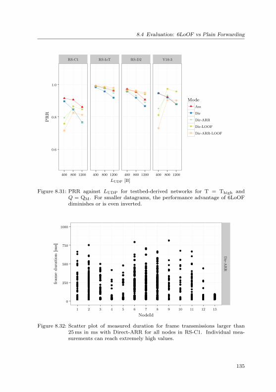
8.4 Evaluation: 6LoOF vs Plain Forwarding
RS-C1 RS-IoT RS-D2 Y10-3
0.6
0.8
1.0
400 800 1200 400 800 1200 400 800 1200 400 800 1200
LUDP [B]
PR
R
ModeAss
Dir
Dir-ARR
Dir-LOOF
Dir-ARR-LOOF
Figure 8.31: PRR against LUDP for testbed-derived networks for T = Thigh andQ = QM. For smaller datagrams, the performance advantage of 6LoOFdiminishes or is even inverted.
0
250
500
750
1000
Dir-A
RR
1 2 3 4 5 6 7 8 9 10 11 12 13
NodeId
fram
edu
rati
on[m
s]
Figure 8.32: Scatter plot of measured duration for frame transmissions larger than25 ms in ms with Direct-ARR for all nodes in RS-C1. Individual mea-surements can reach extremely high values.
135

8 6LoWPAN Ordered Forwarding - 6LoOF
PRR in this scenario by about 0.02. In the light of this observation, choosing the time-out value for forwarding or reassembly based on the size of the incoming datagrampresents an opportunity to improve overall 6LoWPAN performance.
Finally, Fig. 8.31 shows that Direct-LOOF, though being not a rate-restricted for-warding technique, also suffers from a comparatively bad performance for 400 B pack-ets. A possible explanation can be found in the ordering of datagrams. For 400 Bpackets, the transmission rate at the traffic generator is thrice the rate used for 1200 Bpackets, resulting in a larger number of independent packets in the network. Therefore,more fragments are transmitted during the initial probing phase of 6LoOF, increasingthe overall probability of fragments that do not belong to the active datagram to ar-rive at a node. Fragments that do belong to the active datagram, on the other hand,can be delayed by those transmissions. If no fragments of the active datagram areavailable for transmission in such a case, the node remains idle although fragmentsare ready for transmission until the next fitting fragment arrives or the “push back”mechanism described in Sect. 8.1.3 becomes active.
Polling
The results from randomized periodic collection are compared to a straightforwardpolling approach, i.e., the sink asks one node after the other to transmit a UDPpacket. Thereby, contention on the network is reduced to self-interference betweenfragments of the same UDP packet. For these simulation runs, the plain forwardingmodes were used. In all networks, the polling strategy achieves a PRR near one withforwarding modes Assembly and Direct-ARR (not shown). The PRR of the Directmode is lower by a few percent but also above 0.95 in all networks. For each requestedUDP packet, a timeout of 3 s was used. While this may seem a rather large value, thelatency for an individual UDP packet could be observed to occasionally exceed 2 s.
Figure 8.33 shows the average per-node throughput of collecting a single UDP trafficpacket from all nodes in the network. As reference, the average throughput achieved byperiodic push-based collection of data using Direct-ARR-LOOF forwarding is shown.Comparing the average throughput achieved with polling and and push-based collec-tion for the different networks, we see that for the RS-IoT and X3-8 networks, thethroughput is better by about 57 % and 40 %, respectively. In the other networks,polling is outperformed less distinctly (Chain-16, Y3-6, RS-C1) or achieves an evenbetter throughput, albeit with different forwarding modes (Assembly: RS-D1, RS-D2;Direct: Y10-3; Direct-ARR: Y6-4). Achieving a PRR near 1 for T = Tmax, the net-works X3-8, Chain-16 and RS-IoT may support higher traffic rates, while the othernetworks already suffer from congestion for this traffic rate and no further increasecan be expected.
The major difference between the RS-IoT and X3-8 networks, which exhibit thebest performance compared to polling, and all others is, that apart from the lasthop(s), the network can be divided into two spatially divided sub-networks that donot share a common interference range (excluding the last hop towards the gatewaynode). Thereby, transmissions can truly take place in parallel. This is true especiallyfor RS-IoT because even though the potential for pipelining along the same path isexistent, it is limited. This fact can be derived from the only slightly larger throughputachieved by the Direct forwarding modes for polling collection. In this regard, the two
136
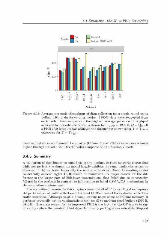
8.4 Evaluation: 6LoOF vs Plain Forwarding
1200
0
1000
2000R
S-C
1
RS-
D1
RS-
D2
RS-
IoT
Cha
in-1
6
Y3-
6
Y6-
4
Y10
-3
X3-
8
Network
b[B
s−1]
ModeAss
Dir
Dir-ARR
Periodic-LOOF-ARR
Figure 8.33: Average per-node throughput of data collection for a single round usingpolling with plain forwarding modes. 1200 B data were requested fromeach node. For comparison, the highest average per-node throughputachieved by periodic collection is shown for LUDP = 1200 B, Q = QM; Ifa PRR of at least 0.9 was achieved the throughput shown is for T = Tmax,otherwise for T = Thigh.
idealized networks with similar long paths (Chain-16 and Y3-6) can achieve a muchhigher throughput with the Direct modes compared to the Assembly mode.
8.4.5 Summary
A validation of the simulation model using two distinct testbed networks shows thatwhile not perfect, the simulation model largely exhibits the same tendencies as can beobserved in the testbeds. Especially the non-rate-restricted Direct forwarding modesconsistently achieve higher PRR results in simulation. A major reason for the dif-ference is the larger part of link-layer transmissions that failed due to consecutivefailures in the testbeds in contrast to failures due to failed CSMA/CA mechanisms inthe simulation environment.
The evaluation presented in this chapter shows that 6LoOF forwarding does improvethe performance of traffic collection in terms of PRR in most of the evaluated collectiontraffic scenarios. Although 6LoOF’s book keeping needs some additional memory, itperforms especially well in configurations with small to medium-sized buffers (2560 B,3840 B). The main reason for the improved PRR is the fact that 6LoOF is able to sig-nificantly reduce the number of link-layer failures by putting nodes into state Stopped
137
8 6LoWPAN Ordered Forwarding - 6LoOF
and thereby reducing the overall contention on the wireless channel. Exemplarily ex-amining the time spent in each state, it could be seen that nodes effectively suspendtheir transmissions in favor of other ongoing transmission. These result clearly indi-cate that the core idea behind the 6LoOF mechanism works well for large datagrams.Furthermore, the results indicate that 6LoOF is at least as fair as the plain Directforwarding modes.
However, there are some drawbacks. Maintaining the same average traffic rate butreducing the payload of individual UDP packets, the advantage that 6LoOF achievesfor very large datagrams diminishes. In some topologies, an significant decrease of thePRR compared to the other forwarding strategies could be observed for a packet sizeof 400 B in combination with a traffic rate near the congestion state of the network.Also, 6LoOF performs slightly worse than the other forwarding modes if the networkis in a congested state.
One of the unsolved problems of 6LoOF is the issue of “snoop-starving” describedin Sect. 8.1.3. Apart from explicitly notifying the predecessors, which necessitateschanges to the 6LoWPAN mechanism, no potential solution to this issue can be pre-sented.
The evaluation also shows that polling is a viable alternative to periodic randomizedpush-based data collection for large datagrams. Especially in networks with no orlimited potential for parallel data transmissions, a simple polling scheme achieves thesame or even slightly better performance than periodically triggered data collection.If, however, potential for parallelization is existent, be it via pipelining on the samepath or segregation of the network into multiple near-independent parts, push-baseddata collection outperforms polling in terms of achievable throughput, which can bealso translated into a larger number of supportable nodes in the network.
138
9 Conclusion and Outlook
The ever increasing demand for ubiquitous autonomously networked sensing and con-trol systems, also known as the “Internet of Things” or “Cyber-Physical Systems”constitutes a number of new challenges. One of those is the question of how to inte-grate large wireless networks of cheap and resource-constrained devices into existingnetwork infrastructures. A proposed solution is to take the proven and time-testedfamily of internet protocols and make them usable on even the tiniest nodes. Severalprotocols that are built upon the internet protocol version 6 have been standardizedby the IETF. Among them, the 6LoWPAN protocol addresses issues of IPv6 headercompression and fragmentation for link-layers that are not capable of providing thefull minimum MTU of 1280 B.
This dissertation addresses the issues that are caused by fragmentation of largedatagrams and their transmission via multi-hop routes using the IEEE 802.15.4 linkand physical layer. It concentrates on data collection traffic scenarios, i.e., multiplenodes, which periodically transmit data to a sink, that utilize the unslotted CSMA/CAmode of the IEEE 802.15.4 MAC protocol. While some research on this topic in formof analytical models and simulative and experimental evaluation exists, the availablework either makes strong simplifications or evaluates the different forwarding strategiesusing unrealistically small networks. Furthermore, the influence of the configurationof underlying link-layer is usually regarded not further. Another proposed approach toimproving 6LoWPAN reliability was based on end-to-end negative acknowledgmentsand can be seen as orthogonal to the research presented here. Taking the effortsfurther, this dissertation makes the following contributions to the problem.
An analytical model based on bit-error probabilities was extended to better reflectpractical approaches to handle the forwarding of fragmented datagrams. By means ofthe extended model, the number of “useless” bits, i.e., data belonging to datagramsthat have already been lost, can be quantified when using a non-reassembling approachto fragment forwarding. The output of the model suggests that for a reasonably highoverall end-to-end datagram success rate, the impact of these already-lost fragmentsis limited. While neglecting important aspects of wireless communication, the modelwas also used to show the strong negative influence the combination of fragmentationand multi-hop transmissions have on the end-to-end datagram success rate.
A suitable simulation model for investigating the performance of 6LoWPAN frag-mentation was discussed. Additionally, a method to derive a network topology includ-ing the link-layer properties from an existing testbed was developed and implementedfor the CometOS framework, which can be used as a basic operating system for wirelesssensor nodes and within the OMNeT++ simulator, using MiXiM to provide the ca-pability of sophisticated modeling of wireless physical channels. By comparing resultsfrom the original testbed and a corresponding testbed-derived simulation environment,a validation of the simulation model could be achieved and thereby the confidence inthe results from the more large-scale simulations could be improved.
139

9 Conclusion and Outlook
With initial experiments and simulations, the two most basic route-over forwardingmodes Assembly and Direct were evaluated together with a forwarding mode whichadaptively restricts the rate of transmissions to prevent self-interference. The re-sults showed a dramatically low PRR especially for the examined Direct forwardingstrategies, whereas the Assembly mode produced results consistent with expectations.Comparing these results to the ones obtained with another model for the bit-errorprobability of the IEEE 802.15.4 layer clearly indicated, that either the simulationdid not generate realistic results or some flaw in the testbed existed. A property ofthe transceiver’s “extended operating mode”, which provides support for automaticCSMA/CA and retransmissions, is that the transceiver becomes incapable of receivingany incoming IEEE 802.15.4 frame as soon as an automatic transmission is initiated.This “no-RX-while-TX” property was finally suspected to be a potential cause for thenon-consistent results.
In consequence, an experiment setup was devised and implemented to quantify theactual influence of the “no-RX-while-TX” property of the transceiver. For this, thedetailed sequence of states of the used radio stack for each of the four participatingnodes was recorded during the transmission of a large datagram along a path of threehops. As a reference, the same experiments were repeated with the radio driver layer ofTinyOS (ported to CometOS) which implements CSMA/CA backoffs and retransmis-sions in software and does allow for the reception of frames during the backoff phase ofa transmission. The obtained results clearly show that the “no-RX-while-TX” prop-erty indeed was solely responsible for the observed results. It has to be noted thatthis finding can be important for all other testbed deployments which use the sametransceiver or a transceiver with a similar mechanism and IEEE 802.15.4’s unslottedCSMA/CA mode. Even though the impact is especially strong in multi-hop scenarioswith fragmentation, it has potential to bias all results taken from deployments usingthis combination. An example for this are M3 OpenNodes running RIOT OS, whichis a probable setup to be encountered in the large and widely-used testbed facilityIoTLab.
After throwing out the transceiver’s extended operating mode, a new parame-ter study was set up with the aim to assess the influence and a suitable set ofIEEE 802.15.4 parameters for 6LoWPAN fragmentation of large datagrams. Further-more, the performance of the different forwarding modes was evaluated for varyingparameter sets, varying backoff exponents, the maximum number of retransmissions,the 6LoWPAN buffer size and the mode of clear channel assessments IEEE 802.15.4uses. The findings of the parameter study include that a larger number of maximumlink-layer retransmissions for all evaluated scenarios improve the overall reliability.Additionally, the IEEE 802.15.4 minimum backoff exponent has a significant influ-ence on the end-to-end datagram success rate. The mode of IEEE 802.15.4 channelassessment does have controversial influence, as the more aggressive variant (mode 3)improved the PRR in a network with artificially increased transmission power but sig-nificantly decreased it for the same routing topology with non-increased transmissionpower. Discussion of the results led to a selection of parameters to be used for theevaluation of the 6LoOF protocol.
Another finding of the evaluation was that a simple polling scheme for certaintopologies proved to be a viable and easy alternative to periodic collection of large dataitems triggered by the nodes independently. In some networks, the polling approach
140

achieves comparable throughput and in nearly all cases a better PRR. The evaluationindicates that polling is viable for large data packets, if the potential for pipelining islimited and no parallel sub-networks exist in the network.
Finally, this dissertation proposes 6LoOF, an implementation of 6LoWPAN thatuses snooping of network traffic to order the transmission of datagrams with the aimto reduces the overall contention for the wireless channel and thereby improve theoverall reliability of the transmission of large, 6LoWPAN-fragmented datagrams. Thebasic idea is that if a node overhears the transmission of a datagram that is not thedatagram currently transmitted by the node itself, the node will suspend its owntransmission to enable fast completion of the overheard datagram. This also impliesan “ordering” of fragments according to their belonging to a certain datagram, whichis reflected in the name of the mechanism. Mechanisms to prevent node starvingand suspension deadlocks were discussed and some additional tweaks to the protocolpresented to improve its performance. 6LoOF was implemented in for CometOS andevaluated in two different testbeds, at the IoTLab and at Hamburg University ofTechnology. Furthermore, a simulation study was carried out, comparing 6LoOF toother forwarding modes in testbed-derived and idealized networks.
The evaluation showed that 6LoOF outperforms the other forwarding modes innearly all of the evaluated scenarios. It consistently was able to reduce the numberof failures at the link-layer that otherwise led to the loss of a whole datagram. Es-pecially with regard to the usage of buffer space, 6LoOF shows that it utilizes theavailable space better than the Assembly mode and works well with small to mediumbuffer sizes. Disabling the optional use of an explicit probing flag by means of a mod-ified header dispatch value, 6LoOF can be implemented completely compliant to the6LoWPAN standard, sacrificing only a tiny part of the reliability improvement.
There are, however, some limitations of the 6LoOF protocol. First, it does not offera significant improvement when smaller datagrams are forwarded. In some cases,especially those of a high traffic load near or in a congested network state, it evenperforms worse for smaller datagrams than the other forwarding modes. Adaptingthe forwarding/reassembly timeout for smaller fragments may mitigate this problem,but not completely. Secondly, one inherent problem of the protocol is its inability fora node to communicate to a predecessor that the datagram belonging to an incomingfragment has been discarded due to a link-layer failure or the lack of buffer space.In consequence, predecessor nodes have to transmit the remaining fragments in aprobing state, wasting much time with an already lost cause. A possible remedy to thissituation is the transmission of explicit notifications every time an invalid fragment isdetected. This approach, however, could not be evaluated in this dissertation, becausethe issue and a possible solution were discovered too late in the process of completion.Finally, it was found that 6LoOF does not perform as well in scenarios with a veryhigh traffic load. The aforementioned issue is likely to be one of the reasons for this.
Applied together with one of the end-to-end congestion control mechanism that areproposed for CoAP to alleviate its shortcomings, the 6LoOF mechanism can be usedto improve the overall reliability in application scenarios that demand for the periodiccollection of large data items using a completely standardized protocol stack.
141

Bibliography
[06] IEEE Standard for Information technology– Local and metropolitan areanetworks– Specific requirements– Part 15.4: Wireless Medium AccessControl (MAC) and Physical Layer (PHY) Specifications for Low RateWireless Personal Area Networks (WPANs). Sept. 2006.
[10] IEC 62591:2010 - Industrial communication networks - Wireless com-munication network and communication profiles - WirelessHARTTM.IEC, 2010.
[11a] IEEE Standard for Local and metropolitan area networks–Part 15.4:Low-Rate Wireless Personal Area Networks (LR-WPANs). Sept. 2011.
[11b] User Manual Radio Modules; deRFmega128-22A00, deRFmega128-22A02, deRFmega128-22C00, deRFmega128-22C02. Document VersionV1.4. dresden electronic. Dresden, Germany, Aug. 2011.
[12a] IEEE 802.15.4eTM-2012 -IEEE Standard for Local and metropolitanarea networks–Part 15.4: Low-Rate Wireless Personal Area Networks(LR-WPANs) Amendment 1: MAC sublayer. IEEE, 2012.
[12b] ZigBee Specification. 2400 Camino Ramon, Suite 375, San Ramon, CA94583: ZigBee Alliance, Sept. 2012.
[14] 8-bit AVR Microcontroller with Low Power 2.4GHz Transceiver for Zig-Bee and IEEE 802.15.4: ATmega256RFR2. Rev. C. Atmel Corporation.San Jose, Sept. 2014.
[15] Low-Power, 2.4 GHz ISM-Band IEEE 802.15.4 RF Transceiver with Ex-tended Proprietary Features: MRF24XA. Rev. C. Microchip TechnologyInc. Chandler, Arizona, Apr. 2015.
[16] IEEE 802.15.4TM-2015 - IEEE Standard for Local and metropolitanarea networks–Part 15.4: Low-Rate Wireless Personal Area Networks(WPANs). IEEE, 2016.
[Adj+15] Cedric Adjih et al. “FIT IoT-LAB: A large scale open experimental IoTtestbed”. In: Internet of Things (WF-IoT), 2015 IEEE 2nd World Fo-rum on. Dec. 2015, pp. 459–464.
[Ali+06] Muneeb Ali, Umar Saif, Adam Dunkels, Thiemo Voigt, Kay Romer, KoenLangendoen, Joseph Polastre, and Zartash Afzal Uzmi. “Medium AccessControl Issues in Sensor Networks”. In: SIGCOMM Comput. Commun.Rev. 36.2 (Apr. 2006), pp. 33–36.
[AMR11] Ahmed Ayadi, Patrick Maille, and David Ros. “TCP over Low-Powerand Lossy Networks: Tuning the Segment Size to Minimize Energy Con-sumption”. In: New Technologies, Mobility and Security (NTMS), 20114th IFIP International Conference on. Feb. 2011, pp. 1–5.
143

Bibliography
[Aya+11] Ahmed Ayadi, Patrick Maille, David Ros, Laurent Toutain, and Pas-cal Thubert. “Energy-efficient fragment recovery techniques for Low-Power and Lossy Networks”. In: Wireless Communications and MobileComputing Conference (IWCMC), 2011 7th International. July 2011,pp. 601–606.
[Bac+12] Nouha Baccour, Anis Koubaa, Luca Mottola, Marco Antonio Zuniga,Habib Youssef, Carlo Alberto Boano, and Mario Alves. “Radio LinkQuality Estimation in Wireless Sensor Networks: A Survey”. In: ACMTrans. Sen. Netw. 8.4 (Sept. 2012), 34:1–34:33.
[Bac+13] Emmanuel Baccelli, Oliver Hahm, Mesut Gunes, Matthias Wahlisch, andThorsten C. Schmidt. “RIOT OS: Towards an OS for the Internet ofThings”. In: Computer Communications Workshops (INFOCOM WK-SHPS), 2013 IEEE Conference on. Apr. 2013, pp. 79–80.
[Bea96] David M. Beazley. “SWIG: An Easy to Use Tool for Integrating ScriptingLanguages with C and C++”. In: Proceedings of the 4th Conference onUSENIX Tcl/Tk Workshop, 1996 - Volume 4. TCLTK’96. Monterey,California: USENIX Association, 1996, pp. 15–15.
[Bet+15] August Betzler, Carles Gomez, Ilker Demirkol, and Josep Paradells. “Co-CoA+: An advanced congestion control mechanism for CoAP”. In: AdHoc Networks 33 (2015), pp. 126–139.
[BGD15] August Betzler, Carles Gomez, and Ilker Demirkol. “Evaluation of Ad-vanced Congestion Control Mechanisms for Unreliable CoAP Communi-cations”. In: Proceedings of the 12th ACM Symposium on PerformanceEvaluation of Wireless Ad Hoc, Sensor, & Ubiquitous Networks.PE-WASUN ’15. Cancun, Mexico: ACM, 2015, pp. 63–70.
[Bia06] Giuseppe Bianchi. “Performance Analysis of the IEEE 802.11 Dis-tributed Coordination Function”. In: IEEE J.Sel. A. Commun. 18.3(Sept. 2006), pp. 535–547.
[Boc+11] Maurizio Bocca, Janne Toivola, Lasse M. Eriksson, Jakko Hollmen, andHeiko Koivo. “Structural Health Monitoring in Wireless Sensor Net-works by the Embedded Goertzel Algorithm”. In: Cyber-Physical Sys-tems (ICCPS), 2011 IEEE/ACM International Conference on. Apr.2011, pp. 206–214.
[BS16] Carsten Bormann and Zach Shelby. Block-wise transfers in CoAP (draft-ietf-core-block-20). https://tools.ietf.org/html/draft-ietf-core-block-20. accessed: 2016-05-11. Apr. 2016.
[Bue+06] Michael Buettner, Gary V. Yee, Eric Anderson, and Richard Han. “X-MAC: A Short Preamble MAC Protocol for Duty-cycled Wireless SensorNetworks”. In: Proceedings of the 4th International Conference on Em-bedded Networked Sensor Systems. SenSys ’06. Boulder, Colorado, USA:ACM, 2006, pp. 307–320.
144

Bibliography
[Cho+09] Aminul Haque Chowdhury, Muhammad Ikram, Hyon-Soo Cha, Has-sen Redwan, S. M. Saif Shams, Ki-Hyung Kim, and Seung-Wha Yoo.“Route-over vs mesh-under routing in 6LoWPAN”. In: Proceedings ofthe 2009 International Conference on Wireless Communications andMobile Computing Connecting the World Wirelessly (IWCMC). 2009,pp. 1208–1212.
[CMN14] Cosmin Cobarzan, Julien Montavont, and Thomas Noel. “Analysis andperformance evaluation of RPL under mobility”. In: 2014 IEEE Sym-posium on Computers and Communications (ISCC). June 2014, pp. 1–6.
[DC12] Stephen Dawson-Haggerty and David E. Culler. BLIP Tutorial. http://tinyos.stanford.edu/tinyos- wiki/index.php/BLIP_Tutorial.accessed: 2016-05-24. 2012.
[De +03] Douglas S. J. De Couto, Daniel Aguayo, John Bicket, and Robert Mor-ris. “A High-throughput Path Metric for Multi-hop Wireless Routing”.In: Proceedings of the 9th Annual International Conference on MobileComputing and Networking. MobiCom ’03. San Diego, CA, USA: ACM,2003, pp. 134–146.
[DGV04] Adam Dunkels, Bjorn Gronvall, and Thiemo Voigt. “Contiki - alightweight and flexible operating system for tiny networked sensors”.In: Local Computer Networks, 2004. 29th Annual IEEE InternationalConference on. Nov. 2004, pp. 455–462.
[Di +12] Piergiuseppe Di Marco, Pangun Park, Carlo Fischione, and Karl Hen-rik Johansson. “Analytical Modeling of Multi-hop IEEE 802.15.4 Net-works”. In: Vehicular Technology, IEEE Transactions on 61.7 (Sept.2012), pp. 3191–3208.
[Dij] Edsger W. Dijkstra. “A note on two problems in connexion with graphs”.In: Numerische Mathematik 1.1 (), pp. 269–271.
[Duq+15] Simon Duquennoy, Beshr Al Nahas, Olaf Landsiedel, and ThomasWatteyne. “Orchestra: Robust Mesh Networks Through AutonomouslyScheduled TSCH”. In: Proceedings of the 13th ACM Conference onEmbedded Networked Sensor Systems. SenSys ’15. Seoul, South Korea:ACM, 2015, pp. 337–350.
[Fam+14] Olivier Fambon, Eric Fleury, Gaetan Harter, Roger Pissard-Gibollet,and Frederic Saint-Marcel. “”FIT IoT-LAB Tutorial: Hands-on PracticeWith a Very Large Scale Testbed Tool for the Internet of Things””. In:10emes journees francophones Mobilite et Ubiquite, UbiMob (2014).
[Gna+09] Omprakash Gnawali, Rodrigo Fonseca, Kyle Jamieson, David Moss,and Philip Levis. “Collection tree protocol”. In: Proceedings of the 7thACM Conference on Embedded Networked Sensor Systems (SenSys ’09).Berkeley, California: ACM, 2009, pp. 1–14.
[GS84] Clark R. Givens and Rae Michael Shortt. “A class of Wasserstein met-rics for probability distributions.” In: Michigan Math. J. 31.2 (1984),pp. 231–240.
145

Bibliography
[Hau09] Jan-Hinrich Hauer. TKN15.4: An IEEE 802.15.4 MAC Implementationfor TinyOS 2. TKN Technical Report Series TKN-08-003. Telecommu-nication Networks Group, Technical University Berlin, Mar. 2009.
[HC08] Jonathan W. Hui and David E. Culler. “Extending IP to Low-Power,Wireless Personal Area Networks”. In: IEEE Internet Computing 12.4(July 2008), pp. 37–45.
[HC11] Ulrich Herberg and Thomas Clausen. “A Comparative PerformanceStudy of the Routing Protocols LOAD and RPL with Bi-directional Traf-fic in Low-power and Lossy Networks (LLN)”. In: Proceedings of the 8thACM Symposium on Performance Evaluation of Wireless Ad Hoc, Sen-sor, and Ubiquitous Networks. PE-WASUN ’11. Miami, Florida, USA:ACM, 2011, pp. 73–80.
[HT11] Jonathan Hui and Pascal Thubert. Compression Format for IPv6 Data-grams over IEEE 802.15.4-Based Networks. RFC 6282. Sept. 2011.
[Ise+15] Javier Isern, August Betzler, Carles Gomez, Ilker Demirkol, and JosepParadells. “Large-Scale Performance Evaluation of the IETF Internet ofThings Protocol Suite for Smart City Solutions”. In: Proceedings of the12th ACM Symposium on Performance Evaluation of Wireless Ad Hoc,Sensor, & Ubiquitous Networks. PE-WASUN ’15. Cancun, Mexico:ACM, 2015, pp. 77–84.
[JDK15] Ilpo Jarvinen, Laila Daniel, and Markku Kojo. “Experimental evaluationof alternative congestion control algorithms for Constrained ApplicationProtocol (CoAP)”. In: Internet of Things (WF-IoT), 2015 IEEE 2ndWorld Forum on. Dec. 2015, pp. 453–458.
[Joh94] Glenn E. Johnson. “Constructions of particular random processes”. In:Proceedings of the IEEE 82.2 (Feb. 1994), pp. 270–285.
[KG14] Hamidreza Kermajani and Carles Gomez. “On the Network Conver-gence Process in RPL over IEEE 802.15.4 Multihop Networks: Improve-ment and Trade-Offs”. In: Sensors (Basel, Switzerland) 14.7 (July 2014),pp. 11993–12022.
[Kim+07a] Sukun Kim, Rodrigo Fonseca, Prabal Dutta, Arsalan Tavakoli, DavidCuller, Philip Levis, Scott Shenker, and Ion Stoica. “Flush: A ReliableBulk Transport Protocol for Multihop Wireless Networks”. In: Proceed-ings of the 5th international conference on Embedded networked sensorsystems. SenSys’07. New York, NY, and USA: ACM, 2007, pp. 351–365.
[Kim+07b] Sukun Kim, Shamim Pakzad, David Culler, James Demmel, GregoryFenves, Steven Glaser, and Martin Turon. “Health Monitoring of CivilInfrastructures Using Wireless Sensor Networks”. In: 2007 6th Interna-tional Symposium on Information Processing in Sensor Networks. Apr.2007, pp. 254–263.
[Ko+10] Teresa Ko, Shaun Ahmadian, John Hicks, Mohammad Rahimi, DeborahEstrin, Stefano Soatto, Sharon Coe, and Michael P. Hamilton. “Heart-beat of a Nest: Using Imagers As Biological Sensors”. In: ACM Trans.Sen. Netw. 6.3 (June 2010), 19:1–19:31.
146

Bibliography
[Kop+08] Andreas Kopke et al. “Simulating Wireless and Mobile Networks in OM-NeT++ the MiXiM Vision”. In: Proceedings of the 1st InternationalConference on Simulation Tools and Techniques for Communications,Networks and Systems & Workshops. Simutools ’08. Marseille, France:ICST (Institute for Computer Sciences, Social-Informatics and Telecom-munications Engineering), 2008, 71:1–71:8.
[Kur+12] Takuto Kuroiwa, Makoto Suzuki, Yasutaka Yamashita, Shunsuke Saru-watari, Tomonori Nagayama, and Hiroyuki Morikawa. “A multi-channelbulk data collection for structural health monitoring using wireless sensornetworks”. In: 2012 18th Asia-Pacific Conference on Communications(APCC). Oct. 2012, pp. 295–299.
[LCC11] Alessandro Ludovici, Anna Calveras, and Jordi Casademont. “Forward-ing Techniques for IP Fragmented Packets in a Real 6LoWPAN Net-work”. In: Sensors 11.1 (2011), pp. 992–1008.
[LCL07] HyungJune Lee, A. Cerpa, and P. Levis. “Improving Wireless SimulationThrough Noise Modeling”. In: Information Processing in Sensor Net-works, 2007. IPSN 2007. 6th International Symposium on. 2007, pp. 21–30.
[Lev+05] Philip Levis et al. “Ambient Intelligence”. In: ed. by Werner Weber, JanM. Rabaey, and Emile Aarts. Berlin, Heidelberg: Springer Berlin Heidel-berg, 2005. Chap. TinyOS: An Operating System for Sensor Networks,pp. 115–148.
[Lev+11] Philip Levis, Thomas Clausen, Jonathan Hui, Omprakash Gnawali, andJeongGil Ko. The Trickle Algorithm. RFC 6206. Mar. 2011.
[Lud+14] Alessandro Ludovici, Piergiuseppe Di Marco, Anna Calveras, and KarlH. Johansson. “Analytical Model of Large Data Transactions in CoAPNetworks”. In: Sensors 14.8 (2014), pp. 15610–15638.
[MLT08] Razvan Musaloiu-E., Chieh-Jan Mike Liang, and Andreas Terzis. “Koala:Ultra-Low Power Data Retrieval in Wireless Sensor Networks”. In: Pro-ceedings of the 7th International Conference on Information Processingin Sensor Networks. IPSN ’08. Washington, DC, USA: IEEE ComputerSociety, 2008, pp. 421–432.
[Mon+07] Gabriel Montenegro, Nandakishore Kushalnagar, Jonathan Hui, and Da-vid Culler. Transmission of IPv6 Packets over IEEE 802.15.4 Networks.RFC 4944. Sept. 2007.
[MT15] Florian Meier and Volker Turau. “An analytical model for fast and verifi-able assessment of large scale wireless mesh networks”. In: Design of Re-liable Communication Networks (DRCN), 2015 11th International Con-ference on the. Mar. 2015, pp. 185–190.
[Nar+07] Thomas Narten, Erik Nordmark, W. Simpson, and Hesham Soliman.Neighbor Discovery for IP version 6 (IPv6). RFC 4944. Sept. 2007.
147
Bibliography
[NH93] Homayoun Nikookar and Homayoun Hashemi. “Statistical modelingof signal amplitude fading of indoor radio propagation channels”. In:Universal Personal Communications, 1993. Personal Communications:Gateway to the 21st Century. Conference Record., 2nd InternationalConference on. Vol. 1. Oct. 1993, 84–88 vol.1.
[Pae+05] Jeongyeup Paek, Krishna Chintalapudi, John Caffrey, Ramesh Govin-dan, and Sami Masri. “A Wireless Sensor Network for Structural HealthMonitoring: Performance and Experience”. In: (2005).
[PG10] Jeongyeup Paek and Ramesh Govindan. “RCRT: Rate-Controlled Reli-able Transport Protocol for Wireless Sensor Networks”. In: ACM Trans-actions on Sensor Networks (TOSN) 7.3 (2010).
[Pos80] John Postel. User Datagram Protocol. RFC 768. Aug. 1980.
[PTB10] Dimosthenis Pediaditakis, Yuri Tselishchev, and Athanassios Boulis.“Performance and Scalability Evaluation of the Castalia Wireless Sen-sor Network Simulator”. In: Proceedings of the 3rd International ICSTConference on Simulation Tools and Techniques. SIMUTools ’10. Torre-molinos, Malaga, Spain: ICST (Institute for Computer Sciences, Social-Informatics and Telecommunications Engineering), 2010, 53:1–53:6.
[Puc+10] Daniele Puccinelli, Omprakash Gnawali, SunHee Yoon, Silvia Giordano,and Leonidas Guibas. “END: A Topology-aware Collection Metric forSensor Networks”. In: Proceedings of the 8th ACM Conference on Em-bedded Networked Sensor Systems. SenSys ’10. Zürich, Switzer-land: ACM, 2010, pp. 419–420.
[Rap02] Theodore S. Rappaport. Wireless communications : principles and prac-tice. 2. ed. Prentice Hall communications engineering and emerging tech-nologies series. Upper Saddle River, NJ: Prentice Hall PTR, 2002.
[Ren13] Bernd-Christian Renner. “Sustained Operation of Sensor Nodes with En-ergy Harvesters and Supercapacitors”. PhD thesis. Hamburg, Germany:Hamburg University of Technology, 2013.
[RH10] George F. Riley and Thomas R. Henderson. “The ns-3 Network Simu-lator”. In: Modeling and Tools for Network Simulation. Ed. by KlausWehrle, Mesut Gunes, and James Gross. Berlin, Heidelberg: SpringerBerlin Heidelberg, 2010, pp. 15–34.
[RL08] Tal Rusak and Philip A. Levis. “Investigating a Physically-based SignalPower Model for Robust Low Power Wireless Link Simulation”. In: Pro-ceedings of the 11th International Symposium on Modeling, Analysis andSimulation of Wireless and Mobile Systems (MSWiM ’08). Vancouver,British Columbia, Canada: ACM, 2008, pp. 37–46.
[Sey05] John S. 1958- Seybold. Introduction to RF propagation. Wiley-Interscience, 2005.
[SHB14] Zach Shelby, Klaus Hartke, and Carsten Bormann. The Constrained Ap-plication Protocol (CoAP). RFC 7252. June 2014.
148

Bibliography
[SK11] Sujesha Sudevalayam and Purushottam Kulkarni. “Energy HarvestingSensor Nodes: Survey and Implications”. In: IEEE Communications Sur-veys Tutorials 13.3 (Third 2011), pp. 443–461.
[SKH06] Dongjin Son, Bhaskar Krishnamachari, and John Heidemann. “Experi-mental Study of Concurrent Transmission in Wireless Sensor Networks”.In: Proceedings of the 4th International Conference on Embedded Net-worked Sensor Systems. SenSys ’06. Boulder, Colorado, USA: ACM,2006, pp. 237–250.
[Sri+10] Kannan Srinivasan, Prabal Dutta, Arsalan Tavakoli, and Philip Levis.“An Empirical Study of Low-power Wireless”. In: ACM Trans. Sen.Netw. 6.2 (Mar. 2010), 16:1–16:49.
[Suz+07] Makoto Suzuki, Shunsuke Saruwatari, Narito Kurata, and HiroyukiMorikawa. “A High-density Earthquake Monitoring System Using Wire-less Sensor Networks”. In: Proceedings of the 5th International Con-ference on Embedded Networked Sensor Systems. SenSys ’07. Sydney,Australia: ACM, 2007, pp. 373–374.
[TB12] Emanuele Toscano and Lucia Lo Bello. “Comparative assessments ofIEEE 802.15.4/ZigBee and 6LoWPAN for low-power industrial WSNs inrealistic scenarios”. In: Factory Communication Systems (WFCS), 20129th IEEE International Workshop on. May 2012, pp. 115–124.
[TH14] Pascal Thubert and Jonathan Hui. LLN Fragment Forwarding and Re-covery (draft). https://tools.ietf.org/html/draft-thubert-6lo-
forwarding-fragments-01. accessed: 2014-09-10. Feb. 2014.
[Thu15] Pascal Thubert. An Architecture for IPv6 over the TSCH mode ofIEEE 802.15.4. http://tools.ietf.org/pdf/draft- ietf- 6tisch-
architecture-09.pdf. accessed: 2016-05-19. Nov. 2015.
[TOV10] Joydeep Tripathi, Jaudelice C. de Oliveira, and Jean-Philippe Vasseur.“A performance evaluation study of RPL: Routing Protocol for Lowpower and Lossy Networks”. In: Information Sciences and Systems(CISS), 2010 44th Annual Conference on. Mar. 2010, pp. 1–6.
[Unt14] Stefan Unterschutz. “Methodologies and Protocols for Wireless Commu-nication in Large-Scale, Dense Mesh Networks”. PhD thesis. Hamburg,Germany: Hamburg University of Technology, 2014.
[UWT12] Stefan Unterschutz, Andreas Weigel, and Volker Turau. “Cross-PlatformProtocol Development Based on OMNeT++”. In: Proceedings of the 5thInternational Workshop on OMNeT++ (OMNeT++’12). Desenzano,Italy, Mar. 2012.
[Var+01] Andras Varga et al. “The OMNeT++ discrete event simulation system”.In: Proceedings of the European simulation multiconference (ESM’2001).Vol. 9. S 185. sn. 2001, p. 65.
[Var99] Andras Varga. “Using the OMNeT++ discrete event simulation systemin education”. In: IEEE Transactions on Education 42.4 (Nov. 1999),p. 372.
149

Bibliography
[VH08] Andras Varga and Rudolf Hornig. “An Overview of the OMNeT++ Sim-ulation Environment”. In: Proceedings of the 1st International Confer-ence on Simulation Tools and Techniques for Communications, Net-works and Systems & Workshops. Simutools ’08. Marseille, France: ICST(Institute for Computer Sciences, Social-Informatics and Telecommuni-cations Engineering), 2008, 60:1–60:10.
[Wat+16] Thomas Watteyne, Vlado Handziski, Xavier Vilajosana, Simon Duquen-noy, Oliver Hahm, Emmanuel Baccelli, and Adam Wolisz. “IndustrialWireless IP-Based Cyber-Physical Systems”. In: Proceedings of the IEEE104.5 (May 2016), pp. 1025–1038.
[Wei+14a] Andreas Weigel, Christian Renner, Volker Turau, and Holger Ernst.“Wireless Sensor Networks for Smart Metering”. In: Energy Conferenceand Exhibition (ENERGYCON), 2014 IEEE International. Dubrovnik,Croatia, May 2014, pp. 722–729.
[Wei+14b] Andreas Weigel, Martin Ringwelski, Volker Turau, and Andreas Timm-Giel. “Route-over forwarding techniques in a 6LoWPAN”. In: EAI En-dorsed Transactions on Mobile Communications and Applications 14.5(Dec. 2014).
[Wei10] Andreas Weigel. “Adaptive Channel Selection in Multi-Gateway WirelessSensor Networks”. MA thesis. Am Schwarzenberg-Campus 3, D-21073Hamburg: Hamburg University of Technology, Aug. 2010.
[Wer+06] Geoffrey Werner-Allen, Konrad Lorincz, Jeff Johnson, Jonathan Lees,and Matt Welsh. “Fidelity and Yield in a Volcano Monitoring SensorNetwork”. In: Proceedings of the 7th Symposium on Operating SystemsDesign and Implementation. OSDI ’06. Seattle, Washington: USENIXAssociation, 2006, pp. 381–396.
[Wes+09] Karl Wessel, Michael Swigulski, Andreas Kopke, and Daniel Willkomm.“MiXiM - The Physical Layer: An Architecture Overview”. In: Proceed-ing of the 2. International Workshop on OMNeT++. Rome, Italy, Mar.2009.
[WGG10] Klaus Wehrle, Mesut Gunes, and James Gross, eds. Modeling and Toolsfor Network Simulation. Springer, 2010.
[Win+12] Tim Winter et al. RPL: IPv6 Routing Protocol for Low-Power and LossyNetworks. RFC 6550. Mar. 2012.
[WPG15] Thomas Watteyne, Maria Rita Palattella, and Luigi Alfredo Grieco. Us-ing IEEE 802.15.4e Time-Slotted Channel Hopping (TSCH) in the In-ternet of Things (IoT): Problem Statement. RFC 7554. May 2015.
[WT14] Andreas Weigel and Volker Turau. “An Analytical Model of 6LoW-PAN Route-Over Forwarding Practices”. In: Conference proceedings ofthe International Conference on Ad-hoc, Mobile and Wireless Networks,ADHOC-NOW 2014. Benidorm, Spain, June 2014, pp. 279–289.
150

Bibliography
[WT15] Andreas Weigel and Volker Turau. “Hardware-Assisted IEEE 802.15.4Transmissions and Why to Avoid Them”. In: Conference proceedings ofthe 8th International Conference on Internet and Distributed ComputerSystems, IDCS 2015. Windsor, UK, Sept. 2015, pp. 223–234.
[WV16] Qin Wang and Xavier Vilajosana. 6top Protocol (6P). http://tools.ietf.org/pdf/draft-ietf-6tisch-6top-protocol-00.pdf. accessed:2016-05-19. Apr. 2016.
[YCI13] Jiazi Yi, Thomas Clausen, and Yuichi Igarashi. “Evaluation of rout-ing protocol for low power and Lossy Networks: LOADng and RPL”.In: Wireless Sensor (ICWISE), 2013 IEEE Conference on. Dec. 2013,pp. 19–24.
[Zhu+13] Yi-Hua Zhu, Gan Chen, Kaikai Chi, and Yanjun Li. “The ChainedMesh-Under Routing (C-MUR) for Improving IPv6 Packet Arrival Rateover Wireless Sensor Networks”. In: Advances in Wireless Sensor Net-works. Vol. 334. Communications in Computer and Information Science.Springer Berlin Heidelberg, 2013, pp. 734–743.
[ZK04] Marco Zuniga and Bhaskar Krishnamachari. “Analyzing the transitionalregion in low power wireless links”. In: Sensor and Ad Hoc Communi-cations and Networks, 2004. IEEE SECON 2004. 2004 First AnnualIEEE Communications Society Conference on. Oct. 2004, pp. 517–526.
151

Glossary
ARQ automatic repeat request
AWGN additive white Gaussian noise
BEP bit error probability
BFSK binary frequency shift keying
CCA clear channel assessment
CoAP Constrained Application Protocol
CSMA/CA carrier sense multiple access with collision avoidance
DCF decider correction factor
DSME distributed synchronous multi-channel extension to IEEE 802.15.4
DSSS direct sequence spread-spectrum
EWMA exponentially weighted moving average
FCF frame control field of the IEEE 802.15.4 MAC header
IEEE 802.15.4 IEEE Standard for Local and metropolitan area networks–Part 15.4:Low-Rate Wireless Personal Area Networks
HTTP Hypertext Transfer Protocol
IETF Internet Engineering Task Force
IPHC 6LoWPAN IPHC header compression
IPv6 Internet Protocol version 6
LFFR LLN fragment forwarding and recovery
LLN low power, lossy network
153
Glossary
6LoOF 6LoWPAN ordered forwarding
6LoWPAN abbreviation for the protocol defined by RFC4944 “Transmission of IPv6Packets over IEEE 802.15.4 Networks”
macCcaMode IEEE 802.15.4 CCA mode (four different variants are specified)
macMinBe IEEE 802.15.4 minimum backoff exponent (unslotted CSMA)
MTU maximum transmission unit
NHC 6LoWPAN next header compression
FEP frame error probability
PRC progress-based retry control
PRR packet success rate
PSDU PHY service data unit
FSP frame success probability
RPL Routing Protocol for Low Power and Lossy Networks
RSSI received signal strength indicator
SFD start of frame delimiter
SINR signal to noise and interference ratio
SNR signal to noise ratio
TCP Transmission Control Protocol
6tisch IPv6 over the TSCH mode of IEEE 802.15.4e
UDP User Datagram Protocol
WSN wireless sensor network
154

List of Symbols
α smoothing factor of EWMA to estimate T tx
BE6LoOF,max maximum backoff exponent of 6LoOF probing mechanism
BE6LoOF,min minimum backoff exponent of 6LoOF probing mechanism
BEmax maximum backoff exponent of unslotted IEEE 802.15.4 CSMA/CA
BEmin minimum backoff exponent of unslotted IEEE 802.15.4 CSMA/CA
c number of correctable bit errors when using forward error correction
EA expectation value of number of bits sent (Assembly)
ED expectation value of number of bits sent (Direct)
EAf expectation value of number of bits sent in case of failure (Assembly)
EAs expectation value of number of bits sent in case of success (Assembly)
Hf,k expectation value of number of bits sent in case of failure on link k
Hp,k expectation value of number of bits sent in case of partial failure on link k
Hs,k expectation value of number of bits sent in case of success on link k
Hsp,k expectation value of number of bits sent in case of success or partial failure onlink k
h index of last hop of a route
h0 index of first hop of a route
htotal accumulated number of hops of all routes in the network participating in thegiven collection traffic pattern
I random part of interval between UDP packet transmissions in traffic generator
i interval between UDP packet transmissions in traffic generator
imax maximum interval between UDP packet transmissions in traffic generator
155

List of Symbols
λ average rate of generation of UDP packets in traffic generator
λB per-node payload data rate in traffic generator
λB,total total raw offered data rate, obtained by the sum of the length of all trafficpaths in the network
LA link layer acknowledgment frame size (bits)
LF link layer frame size (bits), including 802.15.4 headers
l A single path (route) participating in the collection traffic pattern
L Set of all paths used for collection traffic
LUDP payload size of UDP packets in traffic generator
m total number of fragments to transmit
N0 thermal noise power
nf,80 number of sniffer samples with energy above−80 dBm and a foreign IEEE 802.15.4signal being decoded
nf,90 number of sniffer samples with energy between −90 dBm and −80 dBm and aforeign IEEE 802.15.4 signal being decoded
nf,idle number of sniffer samples with energy below−90 dBm and a foreign IEEE 802.15.4signal being decoded
n80 number of sniffer samples with energy above −80 dBm and no IEEE 802.15.4signal
n90 number of sniffer samples with energy between −90 dBm and −80 dBm and noIEEE 802.15.4 signal
nidle number of sniffer samples with energy below −90 dBm
nNSWC,max value of nswc that triggers a node to enter state ProbingBo
no,80 number of sniffer samples with energy above−80 dBm and an internal IEEE 802.15.4signal being decoded
no,90 number of sniffer samples with energy between −90 dBm and −80 dBm and aninternal IEEE 802.15.4 signal being decoded
no,idle number of sniffer samples with energy below−90 dBm and an internal IEEE 802.15.4signal being decoded
156

List of Symbols
nqsa “queue switch after” – number of empty queue object events 6LoOF after which6LoOF switches to the next object in the 6LoWPAN transmission queue
pe bit error probability
pe,frame packet error probability
pe,k bit error probability on link k
Pf,k probability of failure after r attempts on link k
pf,k probability of failure for a single transmission on link k
Ptx transmission power of transceiver
Pp,k probability of partial failure after r attempts on link k
pp,k probability of partial failure for a single transmission on link k
Ps end-to-end probability of success for a whole datagram
Ps,k probability of success after r attempts on link k
ps,k probability of success for a single transmission on link k
QL “large” 6LoWPAN buffer; Q=5120 B or Q=4864 B, depending on forwardingmode
QM “midsize” 6LoWPAN buffer; Q=3840 B or Q=3584 B, depending on forwardingmode
QS “small” 6LoWPAN buffer; Q=2560 B or Q=2304 B, depending on forwardingmode
Q size of the 6LoWPAN buffer
r maximum number of IEEE 802.15.4 retransmissions
Nto timeout counter of aging timeout mechanism
Ito timeout interval of aging timeout mechanism
Tto timeout value of aging timeout mechanism
T categorized traffic load to make different λB comparable for different networks
Tlow traffic category low
Tmid traffic category mid
157
List of Symbols
Thigh traffic category high
Tmax traffic category highest
Ttx average duration of link layer transmissions, including CSMA/CA
Td delay between link layer transmissions
xEPN flag indicating if the explicit probing notification flag, along with a special6LoWPAN header type is used in 6LoOF
158


![Routing Protocol Comparison for 6LoWPAN · PDF fileRouting Protocol Comparison for 6LoWPAN Ki-Hyung Kim ... s a simplified on-demand routing protocol ba sed on AODV[RFC3561] for 6LoWPAN](https://static.fdocuments.us/doc/165x107/5a78c0b07f8b9ae91b8ef859/routing-protocol-comparison-for-6lowpan-protocol-comparison-for-6lowpan-ki-hyung.jpg)