
ROBERTA SCHIATTARELLA - unina.it · dottorato di ricerca in scienze matematiche ciclo xxv sede...
92
DOTTORATO DI RICERCA in SCIENZE MATEMATICHE Ciclo XXV SEDE AMMINISTRATIVA: UNIVERSIT ` A DI NAPOLI FEDERICO II ROBERTA SCHIATTARELLA SOBOLEV AND BOUNDED VARIATION HOMEOMORPHISMS IN R n TESI DI DOTTORATO DI RICERCA TUTORE: COORDINATORE: Ch.mo Prof. Carlo Sbordone Ch.mo Prof. Francesco de Giovanni
Transcript of ROBERTA SCHIATTARELLA - unina.it · dottorato di ricerca in scienze matematiche ciclo xxv sede...

DOTTORATO DI RICERCA
in
SCIENZE MATEMATICHE
Ciclo XXV
SEDE AMMINISTRATIVA: UNIVERSITA DI NAPOLI FEDERICO II
ROBERTA SCHIATTARELLA
SOBOLEV AND BOUNDED VARIATION
HOMEOMORPHISMS IN Rn
TESI DI DOTTORATO DI RICERCA
TUTORE: COORDINATORE:
Ch.mo Prof. Carlo Sbordone Ch.mo Prof. Francesco de Giovanni

2

Contents
1 Lusin’s condition N and related results 9
1.1 Basic properties and definitions . . . . . . . . . . . . . . . . . 9
1.2 Lusin’s condition for Sobolev homeomorphisms . . . . . . . . 18
2 Sobolev and BV homeomorphism: the regularity of the in-
verse. 23
2.1 Bi–Sobolev mappings . . . . . . . . . . . . . . . . . . . . . . . 23
2.2 Regularity of the inverse of a Sobolev homeomorphism with
finite distortion . . . . . . . . . . . . . . . . . . . . . . . . . . 27
2.3 Regularity of the inverse of a homeomorphism of bounded vari-
ation . . . . . . . . . . . . . . . . . . . . . . . . . . . . . . . . 31
2.4 Composition of bi–Sobolev homeomorphisms . . . . . . . . . . 46
3 Some pathological examples of Sobolev homeomorphisms 53
3.1 Sign of the Jacobian . . . . . . . . . . . . . . . . . . . . . . . 53
3.2 Sobolev homeomorphism with zero Jacobian almost everywhere 54
3.3 Bi–Sobolev homeomorphism with zero Jacobian almost every-
where . . . . . . . . . . . . . . . . . . . . . . . . . . . . . . . 57
3

4 On the continuity of the Jacobian of orientation preserving
mappings 71
4.1 The integrability of the Jacobian . . . . . . . . . . . . . . . . 71
4.2 The continuity of the Jacobian . . . . . . . . . . . . . . . . . . 73
4
Introduction
In recent years there has been an increasing interest in the theory of defor-
mations in non linear elasticity. Let us quote here the pioneering works of
Antman, Ball and Ciarlet ([4], [5], [14]).
The domain Ω ⊂ Rn is view as a solid body in the space and the mapping
f : Ω → Rn as a deformation of the body Ω to f(Ω).
The questions that naturally arise are the following:
• Does f satisfy Lusin N condition; i. e. does f map null sets to null
sets? That means, is a “new material ”created from “nothing ”?
• If f is invertible, what are the properties of the inverse map f−1?
• If f is sufficiently smooth, what are the properties of its Jacobian?
The central concept running through all the thesis is the definition of
bi–Sobolev mapping, originally proposed in [48]. We recall that a homeo-
morphism f : Ωonto−→ Ω′ is called a bi–Sobolev mapping if f ∈ W 1,1
loc (Ω,R2)
and its inverse f−1 ∈ W 1,1loc (Ω
′,R2).
The thesis is organized as follows.
In Chapter 1 we recall some definitions and properties of the approximate
gradient of a Borel map. Moreover, we focus our attention on the Lusin N
5

condition and we discuss what kind of mappings satisfy this property. In [78],
Y. G. Reshetnyak showed that every homeomorphism of class W 1,n satisfies
Lusin N condition. An improvement of this result is due to J. Kauhanen, P.
Koskela, and J. Maly ([62]). Using a result of L. Greco ([33]) on the equality
between pointwise and distributional Jacobian, they relaxed the regularity
assumption f ∈ W 1,n into the setting of the closure of W 1,n into the norm
of Grand Sobolev space. We also investigate connections between Lusin N
condition and area formula.
The main topic of Chapter 2 is the regularity of the inverse of Sobolev
and BV homeomorphisms.
In general, one cannot expect the same regularity for f and its inverse.
Indeed, there are examples of Lipschitz homeomorphisms whose inverse are
not in W 1,1loc (see Section 2). In the planar case, S. Hencl, P. Koskela and J.
Onninen in [44] proved that if f : Ωonto−→ Ω′ is a homeomorphism of bounded
variation then so does its inverse map f−1 = (x, y) : Ω′ → Ω. We present a
different proof giving precise formulae for the total variations of the coordi-
nate functions of f−1. Extensions to higher dimension into the Sobolev case
are also considered.
As an application of above results, we study the composition operator of
two Sobolev homeomorphisms. Some of these results can be found in [18],
[22], [35].
In Chapter 3 we investigate how big can be the zero set of the Jacobian de-
terminant of a homeomorphism f . The null set of the Jacobian determinant
of a bi–Sobolev map could have positive measure (see [53], Section 6.2.6).
Moreover, we are able to construct for n ≥ 3 a pathological example of a
6

bi–Sobolev map with Jf = Jf−1 = 0 almost everywhere. Such a pathological
homeomorphism cannot exists in dimension n = 2 or with higher regularity
f ∈ W 1,n−1 (see [19]).
In the last Chapter we investigate the continuity in L1 norm of the Ja-
cobian determinant of orientation preserving maps belonging to the Grand
Sobolev space W 1,n)(Ω,Rn). Let us recall that if Jf ≥ 0 a.e., then |Df | ∈
Ln)(Ω) is the weakest assumption to guarantee that Jf is locally integrable
(see [55]).
7

8

Chapter 1
Lusin’s condition N and related
results
The main topic of this chapter is the study of Lusin’s condition N . We focus
our attention on some of its consequences and then investigate what are
the minimal integrability conditions on the partial derivatives of a Sobolev
homeomorphism f ∈ W 1,1loc (Ω,R
n) needed to guarantee that f satisfies it.
1.1 Basic properties and definitions
Let Ω be a bounded domain in Rn and f : Ω → R
n a mapping of the Sobolev
classW 1,p(Ω,Rn) . Here,W 1,p(Ω,Rn) consists of all p-integrable mappings of
Ω into Rn whose coordinate functions have p-integrable distributional deriva-
tives.
We denote by Df(z) the differential matrix of f at the point z ∈ Ω and
9

by Jf (z) the Jacobian determinant of Df :
Jf (z) = detDf(z).
The norm of Df(z) is defined as follows:
|Df(z)| = supξ∈Rn,|ξ|=1
|Df(z)ξ|.
It is easy to see that other norms are equivalent.
We need to recall the definition of approximate gradient of a Borel map
(see [32]).
For any measurable set A ⊂ Rn, the upper density θ∗(A, z) of A at z is
defined as
lim supr→0
|B(z, r) ∩ A||B(z, r)| .
Similarly, the lower density θ∗(A, z) of A at z is given by
lim infr→0
|B(z, r) ∩ A||B(z, r)| .
The density of A at z is defined whenever θ∗(A, z) = θ∗(A, z) as the common
value:
θ(A, z) = θ∗(A, z) = θ∗(A, z).
Let u : Ω −→ R be a measurable function. We recall that l is the
approximate limit of u at z when ρ tends to z in Ω, and we write
l = ap limρ→z
u(ρ)
10
if for all ε > 0, the set
Ωε = ρ ∈ Ω | |u(ρ)− l| ≥ ε
has density 0 at z.
The approximate upper limit of u at z is defined as the number (eventually
+∞ or −∞) given by
ap lim supρ→z
u(ρ) = inft | θ∗(E+t , z) = 0
where E+t = z ∈ Ω|u(z) > t.
Similarly, the approximate lower limit is given by
ap lim infρ→z
u(ρ) = supt|θ∗(E−t , z) = 0
where E−t = z ∈ Ω|u(z) < t.
Of course,
ap lim infρ→z
u(ρ) ≤ ap lim supρ→z
u(ρ)
and whenever
ap lim infρ→z
u(ρ) = ap lim supρ→z
u(ρ) = l ∈ R
the approximate limit exists and we have
ap limρ→z
u(ρ) = l.
11

We say that u : Ω −→ R is approximately continuous at z if
u(z) = ap limρ→z
u(ρ).
One can also prove
Proposition 1.1. If the function u : Ω −→ R is measurable then u is ap-
proximately continuous at a.e. z ∈ Ω.
The previous Proposition is an easy consequence of the Lebesgue dif-
ferentation theorem in the case of L1 maps. We have in fact
Proposition 1.2. Let u ∈ L1loc(Ω). If there exists τ ∈ R such that
limr→0
∫
Br(z)
|u(ρ)− τ |dρ = 0 (1.1)
then,
ap limρ→z
u(ρ) = τ. (1.2)
In particular, as a consequence, the approximate limit exists at each
Lebesgue point z.
In the same spirit of approximate limits and approximate continuity, we
may now introduce the notion of approximate differential.
Definition 1.1. Let Ω be a measurable subset of Rn and u : Ω → R be a
measurable map. Suppose that z ∈ Rn be such that θ∗(A, z) > 0. We say
that u is approximately differentiable at z if there exists a linear mapping
12

L : Rn −→ R such that:
ap lim supρ→z
|u(ρ)− u(z)− L(ρ− z)||ρ− z| = 0.
From the definition, it is not difficult to show that the approximate dif-
ferential, denoted by apDu(z) is unique whenever it exists.
Theorem 1.1. Assume u ∈ W 1,1loc (R
n). Then u is approximately differen-
tiable a.e. and its approximate derivative equals its weak derivative a.e.:
apDu(z) = Du(z) a. e.
In geometric function theory we are interested in the study of mappings
and their properties. One of the most important properties is the following:
Definition 1.2. Let f : Ω → Rn be a measurable mapping. We say that f
satisfies Lusin’s condition N if for each E ⊂ Ω,
|E| = 0 ⇒ |f(E)| = 0.
This property has the following physical interpretation. If we imagine
that Ω is a body in the space that is subjected to a deformation f , “new
material”cannot be crated from “nothing ”.
For the sake of completeness we review some of the standard results to-
gether with their proofs.
Let Ω and Ω′ be bounded domains in Rnand let us denote by Hom(Ω,Ω′)
the set of all homeomorphisms f : Ω → Ω′ = f(Ω).
13
Proposition 1.3. f ∈ Hom(Ω,Ω′) satisfies Lusin’s condition N if, and only
if, f takes measurable sets to measurable sets.
Proof. Let us assume that f satisfies the condition N . If A ⊂ Ω is a measur-
able set, then there exists a Borel set B such that B ⊂ A ⊂ Ω and |B\A| = 0.
Then we have |f(B\A)| = |f(B)\f(A)| = 0 and hence f(B)\f(A) is measur-
able. Moreover, as f is a homeomorphism, f(B) is a Borel set and hence f(A)
is also measurable. Conversely, by contradiction suppose that E ⊂ Ω verifies
|E| = 0 and |f(E)| > 0. If A′ ⊂ f(E) is a non measurable set then, f−1(A′)
is a measurable set of measure zero. By assumption also A′ = f(f−1(A′)) is
measurable as well and there is a contradiction.
Proposition 1.4. f ∈ Hom(Ω,Ω′) satisfies Lusin’s condition N if, and only
if, |f(E)| = 0 whenever E ⊂⊂ Ω is a compact set with zero measure.
Proof. Let E be a compact set with zero measure such that |f(E)| = 0. Then,
there exists a Borel set B ⊃ E such that |B| = 0. Suppose by contradiction
that |f(B)| > 0. Hence, there exists a compact set C ′ ⊂ f(B) such that
|C ′| = |f(B)| > 0. But f is a homeomorphism and f−1(C ′) is compact and
|f−1(C ′)| ≤ |B| = 0. This is not possible by assumption.
The condition N is strongly connected with the validity of the area for-
mula which is crucial in the next developments. An advanced version of the
theorem on change of variables is due to Federer [ [25], Theorem 3.2.3]. It
states that the area formula:
∫
Ω
η(f(z))|Jf (z)| dz =∫
Rn
(
∑
z∈Ω: f(z)=w
η(w)
)
dw (1.3)
14
is valid for all measurable functions η : Rn −→ [0,+∞), if f is a Lipschitz
map.
By Theorem 1.1, the set of points of approximate differentiable of f
AD(f) = z ∈ Ω | f is approximately differentiable atz
is a set of full measure.
Let us consider the set:
AL(f) =
z ∈ Ω∣
∣
∣ap lim sup
w→z
|f(w)− f(z)||w − z| <∞
.
Trivially, AD(f) ⊂ AL(f). By Theorem 3.1.8 of [25] , AD(f) is the union of
a countable family of measurable sets such that the restriction of f to each
member of the family is Lipschitz and hence the formula (1.3) becomes:
∫
Ω
η(f(z))|Jf (z)| dz ≤∫
Rn
(
∑
z∈Ω: f(z)=w
η(w)
)
dw (1.4)
Moreover, in (1.4), there is an equality if f satisfies Lusin’s condition N .
Notice that the area formula holds on the set where f is approximately
differentiable; in fact, the Lusin’s condition N holds on AD(f).
From (1.4), we can derive the following:
Theorem 1.2 (Area formula for Sobolev homeomorphisms). Let f : Ω −→
Rn be a Sobolev homeomorphism, η : Rn −→ [0,+∞) be a nonnegative Borel
measurable function and A be a Borel measurable set. Then:
∫
A
η(f(z))|Jf (z)| dz ≤∫
f(A)
η(w) dw. (1.5)
15

The equality:∫
A
η(f(z))|Jf (z)| dz =∫
f(A)
η(w) dw (1.6)
is verified if f satisfies Lusin’s condition N .
When (1.6) occurs we say that the area formula holds for f on A.
We note the following consequence of (1.5). If A′ ⊂ f(A) is a Borel subset
with |A′| = 0, then Jf (z) = 0 for a.e. z ∈ f−1(A′). Indeed,
∫
f−1(A′)
|Jf (z)| dz ≤∫
A′
dw = |A′| = 0.
Moreover, it is well known that there exists a set Ω ⊂ Ω of full measure
|Ω| = |Ω|, such that:
∫
Ω
η(f(z))|Jf (z)| dz =∫
f(Ω)
η(w) dw. (1.7)
As a consequence, if f is a Sobolev homeomorphism with f−1 satisfying the
N , then Jf (z) > 0 for almost every z ∈ Ω. Indeed, by (1.7),
|f(
z ∈ Ω : Jf (z) = 0)
| = 0.
Hence, by the N for f−1 and since Ω has full measure:
|z ∈ Ω : Jf (z) = 0| = |(
z ∈ Ω : Jf (z) = 0)
∪(
Ω \ Ω)
| = 0.
Thus in particular, as AD(f) is a set of full measure, the image of the set
16

of all critical points has zero measure:
|f (z ∈ Ω : f is approximately differentiable at z and Jf (z) = 0) | = 0.
This is a weak version of the classical Sard theorem.
An interesting application of condition N is the following result on the
inverse of an a.e. approximately differentiable homeomorphism.
Proposition 1.5. Let f ∈ Hom(Ω;Ω′) be approximately differentiable a.e..
If f verifies Lusin’s condition N , then the inverse f−1 is approximately dif-
ferentiable a.e.
Proof. We decompose the set AD(f) of points of approximately differentiable
of f as follows:
AD(f) = Rf ∪ Zf
where
Rf = z ∈ Ω : f is approximately differentiable at z and Jf (z) 6= 0
and
Zf = z ∈ Ω : f is approximately differentiable at z and Jf (z) = 0 .
Moreover, we consider
Ef = z ∈ Ω : f is not approximately differentiable at z
17

and hence
Ω = Zf ∪Rf ∪ Ef .
By the weak version of the classical Sard Lemma, |f(Zf )| = 0. Since f−1 is
approximately differentiable a.e., Ef has zero measure and by condition N ,
f(Ef ) has zero measure.
We notice that f−1 is approximately differentiable in f(Rf ) which is a
subset of full measure of f(Ω); indeed,
f(Ω) \ f(Rf ) = f(Zf ) ∪ f(Ef )
has zero measure.
1.2 Lusin’s condition for Sobolev homeomor-
phisms
We study conditions under which a map f could satisfy Lusin’s condition N .
Firstly, we consider the case of real- valued functions. A function f is
called absolutely continuous in a set E if the following condition is satisfied:
for every ε > 0, there exists δ = δ(ε) > 0 such that
N∑
i=1
|f(bi)− f(ai)| < ε
18

for every collection (ai, bi) of pairwise disjoint intervals with
N∑
i=1
(bi − ai) < δ.
An absolutely continuous function clearly satisfies Lusin’s condition N and
hence also every Lipschitz function sends sets of measure zero to sets of
measure zero. We note that by Rademacher’s theorem, locally Lipschitz
functions are differentiable almost everywhere. However, differentiability a.e.
is not enough to conclude Lusin’s condition N (see for example the Cantor
function).
In dimension n ≥ 2, the situation is much more complicated. M. Mar-
cus and V. Mizel, in [67], proved that Lusin’s condition N holds if f is a
continuous map in W 1,p provided p > n. The Lusin condition may fail for
continuous mappings inW 1,n. L. Cesari ([13]) demonstrated that there exists
a continuous map f ∈ W 1,n([−1, 1]n, [−1, 1]n) with n ≥ 2 such that
f(
[−1, 1]× 0n−1)
= [−1, 1]n
and hence f does not satisfy the Lusin’s condition N . Moreover, in the paper
[68], O. Martio and W. Ziemer investigated how condition N is related to
mappings in the Sobolev space W 1,n(Ω,Rn) with nonnegative Jacobians. In
particular, they showed that if f is a continuous map in W 1,n(Ω,Rn) with
Jf > 0 a.e. on Ω then, f satisfies Lusin’s condition N .
For a homeomorphism, less regularity is needed: it suffices to assume that
f ∈ W 1,nloc
(Ω,Rn). This is due to Reshetnyak ([77]). This result is sharp in
19

the scale ofW 1,p(Ω,Rn) - homeomorphisms. In fact, in the case p < n, Pono-
marev showed in [76], that for every n > 1 there exists a homeomorphism
f : [0, 1]n −→ [0, 1]n such that:
• the restriction of f to the boundary of the cube [0, 1]n is the identity
mapping;
• for all 0 < p < n, f belongs to the class W 1,p([0, 1]n, [0, 1]n);
• f does not have property N ;
• the inverse map f−1 belongs to the class W 1,p([0, 1]n, [0, 1]n) with any
1 < p <∞.
Another example has been constructed in [62] of a homeomorphism f ∈
∩1≤p<nW1,p(Ω,Rn) satisfying the condition
sup0<ε≤n−1
ε
∫
Ω
|Df |n−ε <∞ (1.8)
and such a mapping f does not satisfy condition N .
Let us define the Grand Lebesgue space Ln)(Ω) as the collection of all
measurable functions u with
‖u‖n) = sup0<ε≤n−1
(
ε
∫
Ω
|u(z)|n−ε dz
) 1n−ε
<∞.
This Banach space was introduced in [55] for mappings f : Ω ⊂ Rn → R
n (not
necessarily homeomorphisms) in the study of the integrability of nonnegative
Jacobians under minimal integrability assumptions for |Df |.
20

We also mention the article [62] by J. Kauhanen, P. Koskela and J. Maly,
where it is shown that the sharp regularity assumption to rule out the failure
of the condition N can be the following one:
limε→0+
ε
∫
Ω
|Df |n−ε = 0 (1.9)
under the condition that the Jacobian determinant is non negative a.e..
When (1.9) occurs, we write |Df | ∈ Ln)b (Ω). This function space is the
closure of bounded functions in Ln) (see [33]). Moreover, the following inclu-
sions hold:
Ln)b (Ω) ⊂ Ln)(Ω) ⊂
⋂
p<n
Lp(Ω).
We want underline that if |Df | ∈ Ln)b then, the weak Jacobian of the mapping
f coincides with the pointwise Jacobian by a result of L. Greco (see [33]).
Let us now introduce a space slightly larger than Ln(Ω) and then we shall
examine some relations between Ln)b and other classes of functions.
Our main source here will be [53, Section 4.12]. We shall need to consider
the Zygmund space Lp logα L(Ω), for 1 6 p < ∞, α ∈ R (α > 0 for p = 1),
and Ω ⊂ Rn. This is the Orlicz space generated by the function
Φ(t) = tp logα(a+ t) , t > 0 ,
where a > 0 is a suitably large constant, so that Φ is increasing and convex
on [0,∞[. The choice of a will be immaterial, as we shall always consider
these spaces on bounded domains. Thus, more explicitly, for a measurable
21
function u on Ω, u ∈ Lp logα L(Ω) simply means that
∫
Ω
|u|p logα(a+ |u|) dx <∞ .
As an example, for α = 0 we have the ordinary Lebesgue spaces. We shall
consider in Lp logα L(Ω) the Luxemburg norm
‖u‖Lp logα L = inf
λ > 0 :
∫
Ω
Φ(|u|/λ) dx 6 1
.
The following Holder type inequality for Zygmund spaces will be important
to us:
‖u1 · · · uk‖Lp logα L 6 C ‖u1‖Lp1 logα1 L · · · ‖uk‖Lpk logαk L (1.10)
where pi > 1, αi ∈ R, for i = 1, . . . , k, and
1
p=
1
p1+ · · · 1
pk,
α
p=α1
p1+ · · · αk
pk
The positive constant C in (1.10) is independent of ui.
We shall write u ∈ Lp logα Lloc(Ω) if u ∈ Lp logα L(E), for every compact
subset E of Ω.
For the Zygumund spaceLn
logL, the following inclusions hold:
Ln ⊂ Ln
logL⊂ Ln
b ⊂ Ln).
(see [33]).
22

Chapter 2
Sobolev and BV
homeomorphism: the regularity
of the inverse.
This chapter is concerned with the regularity of the inverse of a homeomor-
phism f of bounded variation in the planar case. We give precise formulae
for the total variations of the coordinate functions of f−1. Extensions to
higher dimension are also given.
2.1 Bi–Sobolev mappings
Let Ω and Ω′ be domains in R2. Recently, the relation between a homeo-
morphism f : Ω −→ Ω′ and its inverse has been intensively studied (see [43],
[45], [48]).
In the class of planar homeomorphisms a crucial role is played by bi–
23

Sobolev mappings, originally proposed in [48]. We recall that a homeomor-
phism f : Ωonto−→ Ω′ is called a bi–Sobolev mapping if f ∈ W 1,1
loc (Ω,R2) and
its inverse f−1 ∈ W 1,1loc (Ω
′,R2).
A first interesting property of a bi–Sobolev map f = (u, v) in the plane
is that u and v have the same critical points.
Theorem 2.1. Let f = (u, v) : Ωonto−→ Ω′ be a bi–Sobolev map. Then u and
v have the same critical points:
z ∈ Ω | ∇u(z) = 0 = z ∈ Ω | ∇v(z) = 0 a. e.
The same result holds also for the inverse.
The connection between the planar elliptic PDE’s and Function Theory
has been known since pioneering works of .B. Morrey [71], R. Caccioppoli
[11], L. Bers and L. Nirenberg [10], I.N. Vekua [81] and B. Bojarski [7] (see
also ([3],[65]).
A homeomorphism f = (u, v) : Ω −→ R2 is K–quasiconformal mapping
for a constant K ≥ 1, if f ∈ W 1,2loc (Ω,R
2) and
|Df(z)|2 ≤ KJf (z) a.e. z ∈ Ω. (2.1)
The smallest constant K for which (2.1) holds almost everywhere is called
the distortion of the mapping f .
Quasiconformal mappings possess many interesting properties, as embod-
ied in the following
Theorem 2.2. Let f : Ω −→ Ω′ be a K– quasiconformal mapping and let
24

g : Ω′ −→ R2 a K ′– quasiconformal mapping. Then
• f−1 : Ω′ → Ω is K– quasiconformal
• g f : Ω → R2 is KK ′– quasiconformal
• f satisfy the Lusin’s condition N
• the Jacobian determinant Jf (z) > 0 almost everywhere in Ω.
Some results hold also when the distortion K = K(z) is not bounded. A
mapping f ∈ W 1,1loc (Ω,R
n) is said to have finite distortion if there exists a
measurable function K : Ω −→ [1,∞) such that
|Df(z)|n 6 K(z) Jf (z) . (2.2)
Moreover, we assume that Jf ∈ L1loc(Ω).
We note that the existence of a measurable function K finite a.e. and
satisfying (2.2) amounts to saying that
Jf (z) = 0 =⇒ Df(z) = 0 a.e. (2.3)
This condition makes it possible to consider the distortion quotient
|Df(z)|nJf (z)
for a.e. z ∈ Ω. (2.4)
Hereafter the undetermined ratio 00is understood to be equal to 1 for z in
25

the zero set of the Jacobian:
Kf (z) =
|Df(z)|nJf (z)
, if Jf (z) > 0 ;
1 , otherwise.
(2.5)
In other words, Kf is the smallest function greater than or equal to 1 for
which (2.2) holds a.e.
It is well known (see [57]) that if f = (u, v) is a K–quasiconformal map
then u and v lie in W 1,2(Ω) and satisfy the same elliptic equation
divA(z)∇u = 0 and divA(z)∇v = 0 (2.6)
where A = A(z) ∈ L∞(Ω,R2 × R2) is a symmetric matrix with detA = 1
satisfying the uniform ellipticity bounds
|ξ|2K
≤ 〈A(z)ξ, ξ〉 ≤ K|ξ|2.
If f = (u, v) is only a bi–Sobolev homeomorphism, there is also an inter-
play with the solutions of (2.6) in the sense of distributions. Indeed, it was
shown in [43] and [15] that each bi-Sobolev mapping in dimension n = 2 has
finite distortion and in [48], it was shown that for any such f = (u, v) there
corresponds a degenerate elliptic matrix A = Af (z) with eigenvalues in the
interval
[
1
K(z), K(z)
]
such that u and v are very weak solutions to (2.6),
i.e. u, v ∈ W 1,1 satisfy (2.6) in the sense of distributions.
Theorem 2.3. To each bi–Sobolev mapping f = (u, v) : Ω → Ω′, there
26

corresponds a measurable function A = A(z) valued in symetric matrices
with detA(z) = 1 that for a.e. z ∈ Ω and for all ξ ∈ R2 we have
|ξ|2K(z)
≤ 〈A(z)ξ, ξ〉 ≤ K(z)|ξ|2.
where K(z) denotes the distortion function of f . The components of f are
very weak solutions of equation (2.6) with finite energy, i.e.
∫
Ω
〈A(z)∇u,∇u〉 <∞ and
∫
Ω
〈A(z)∇v,∇v〉 <∞.
Another important property of bi-Sobolev mappings is the following (see
[43], [48])
Theorem 2.4. Let f : Ω → Ω′ be a bi-Sobolev mapping. Then
∫
Ω
|Df(z)| dz =∫
Ω′
|Df−1(w)| dw. (2.7)
2.2 Regularity of the inverse of a Sobolev home-
omorphism with finite distortion
A part of the study of mappings of finite distortion which is vital to us is the
regularity of the inverse of a Sobolev homeomorphism, see [15, 43, 44, 48, 74,
28].
The bi-Sobolev assumption rules out a large class of homeomorphisms.
In fact, it is possible to construct a homeomorphism f : R2 −→ R2 such
that f is Lipschitz, but the inverse f−1 does not belong to W 1,1loc (R
2,R2). For
27

example, the mapping
f0 : (0, 2)× (0, 1)onto−→ (0, 1)× (0, 1) f0(x, y) = (h(x), y) (2.8)
where h−1(t) = t + c(t) and c : (0, 1) → (0, 1) is the usual Cantor ternary
function, is a Lipschitz homeomorphism whose inverse f−10 does not belong
to W 1,1loc .
Notice that Jf0(z) vanishes in a set of positive area. In fact, a sufficient
condition under which the inverse of a Sobolev homeomorphism belongs to
W 1,1loc is that Jf > 0 a.e. (see theorem 1.1 of [43]). But, it is not a necessary
condition. Indeed, it is possible to construct a bi–Sobolev homeomorphism
such that Jf = 0 in a set of positive area (see [53], Section 6.5.6).
A necessary and sufficient condition for f−1 ∈ W 1,1loc (R
2,R2) is thatDf(z) =
0 almost everywhere in the set z : Jf (z) = 0, i. e. that f has finite distor-
tion (see [43] and [41]).
Theorem 2.5. Let Ω,Ω′ be planar domains and f : Ω → Ω′ be a Sobolev
homeomorphism. Then, the following conditions are equivalent:
• f−1 ∈ W 1,1loc (R
2,R2)
• f has finite distortion
• f−1 has finite distortion.
A suitable integrability condition on the distortion function K guarantees
a better regularity for the inverse.
28

Theorem 2.6. Let Ω ⊂ R2 be a domain. If f : Ω → R
2 is a Sobolev homeo-
morphism of finite distortion K ∈ L1(Ω), then f−1 belongs to W 1,2loc (f(Ω),R
2)
and is a mapping of finite distortion.
We want underline that an integrability assumption of K1−δ for 0 < δ < 1
does not give any better than W 1,1–regularity of f−1. Hereafter, we use the
notation Q0 = [0, 1]× [0, 1] for the unit square in R2.
Example 2.1. Let 0 < δ < 1. There is a homeomorphism f : Q0 → Q0
of finite distortion such that f ∈ W 1,1loc (Q0,R
2), K1−δ ∈ L1(Q0) but f−1 /∈
W 1,1loc (Q0,R
2).
In higher dimension, besides the outer distortion already introduced in
Section 2.1, we shall need to consider the inner distortion. A mapping
f ∈ W 1,1loc (Ω;R
n) has finite inner distortion if its Jacobian Jf ∈ L1loc(Ω),
Jf ≥ 0 a.e. and
Jf (z) = 0 =⇒ | adjDf(z)| = 0 a.e. ,
where adjDf is the adjugate of the differential matrix Df of f .
For such a map, we call inner distortion of f the smallest function KIf > 1
such that
| adjDf(z)|n 6 KIf (z) Jf (z)
n−1 , (2.9)
for a.e. z ∈ Ω. Clearly, a map of finite outer distortion has also finite inner
distortion and KIf 6 (Kf )
n−1, as a consequence of Hadamard’s inequality
(| adjDf | ≤ |Df |n−1). In dimension n = 2 the two notions coincide.
29

Let us give the statement analogous to planar case examined in Theorem
2.5.
Theorem 2.7 ([28]). Let f : Ωonto−→ Ω′ be a homeomorphism inW 1,n−1
loc(Ω,Rn)
with finite inner distortion. Then, f−1 is a W 1,1loc
(Ω′,Rn) mapping of finite
distortion. Moreover,
|Df−1(w)|n ≤ K(f−1(w))Jf−1(w) for a.e. w ∈ Ω′, (2.10)
and∫
Ω′
|Df−1(w)|dw =
∫
Ω
| adjDf(z)|dz.
The same conclusion was known by M. Csornyei, S. Hencl, J. Maly [15]
under the strong assumption that f has finite outer distortion.
The regularity assumption |Df | ∈ Ln−1loc cannot be weakened in the scale
of Sobolev space. In fact, it is possible to construct a homeomorphism f ∈
W 1,n−1−ε where 0 < ε < 1 such that | adjDf | ∈ L1(Ω) but f−1 /∈ W 1,1,loc . The
above theorem is also sharp in the setting of Orlicz space (see [39]).
Regarding the higher dimensional setting, in [48] the authors showed:
Theorem 2.8. Let n ≥ 2 and let f : Ω → Rn be a bi–Sobolev map. Suppose
that for a measurable set E ⊂ Ω we have Jf = 0 almost evrywhere on E.
Then, | adjDf | = 0 a.e. on E. If we moreover assume that Jf ≥ 0, it follows
that f has finite inner distortion.
For n > 2 a similar result of Theorem 2.6 has been established in [72].
Theorem 2.9. Let Ω,Ω′ be bounded domains in Rn and f ∈ W 1,n−1 be a
homeomorphism with finite inner distortion such that KIf ∈ L1(Ω). Then,
30

|Df−1| ∈ Ln(Ω′) and
∫
Ω′
|Df−1(w)|ndw =
∫
Ω
KIf (z)dz.
In [72], it is worth pointing out that the regularity of the distortion influ-
ences the regularity of the inverse mapping also in the scale of Orlicz space.
2.3 Regularity of the inverse of a homeomor-
phism of bounded variation
Let Ω be a domain in R2. A function u ∈ L1(Ω) is of bounded variation,
u ∈ BV(Ω), if the distributional partial derivatives of u are measures with
finite total variation in Ω: there exist Radon signed measures D1u, D2u in
Ω such that for i = 1, 2, |Diu|(Ω) <∞ and
∫
Ω
uDiφ(z) dz = −∫
Ω
φ(z) dDiu(z) ∀φ ∈ C10(Ω).
The gradient of u is then a vector-valued measure with finite total variation
|∇u| (Ω) = sup
∫
Ω
udivϕ(z) dz : ϕ ∈ C10(Ω,R
2), ‖ϕ‖∞ ≤ 1
<∞.
By |∇u| we denote the total variation of the signed measure Du.
The Sobolev space W 1,1(Ω) is contained in BV(Ω); indeed for any u ∈
W 1,1(Ω) the total variation is given by∫
Ω|∇u| = |∇u| (Ω).
31
We say that f ∈ L1(Ω;Rn) belongs to BV(Ω;Rn) if each component of f is
a function of bounded variation. Finally we say that f ∈ BVloc(Ω;Rn) if f ∈
BV(A;Rn) for every open A ⊂⊂ Ω. In the following, for f ∈ BVloc(Ω;Rn)
we will denote the total variation of f by:
|Df | (Ω) = sup
n∑
i=1
∫
Ω
fidivϕi(z) dz : ϕi ∈ C10(Ω;R
n), ‖ϕi‖∞ ≤ 1, i = 1, . . . , n
.
The space BV(Ω,Rn) is endowed with the norm
‖f‖BV :=
∫
Ω
|f(z)| dz + |Df |(Ω).
There are equivalent ways to define a norm for BV maps. For example,
|f |BV(Ω) = sup
∣
∣
∣
∣
∫
Ω
[DTϕ(z)]f(z) dz
∣
∣
∣
∣
and the supremum runs over all test mappings ϕ ∈ C∞0 (Ω,Rn) with ‖ϕ‖∞ =
1.
We will need the definition of sets of finite perimeter (see [1]).
Definition 2.1. Let E be a Lebesgue measurable subset of Rn. For any open
set Ω ⊂ Rn the perimeter of E in Ω, denoted by P (E,Ω), is the total variation
of χE in Ω, i.e.
P (E,Ω) = sup
∫
E
divϕdz : ϕ ∈ C10(Ω;R
n), ‖ϕ‖∞ ≤ 1
.
We say that E is a set of finite perimeter in Ω if P (E,Ω) <∞.
32

Lemma 2.1. For any open set Ω′ ⊂ Rn and xi ∈ L1
loc(Ω′) we have
|∇xi| (Ω′) =
∫ +∞
−∞P (w ∈ Ω′ : xi(w) > t ,Ω′) dt. (2.11)
It is a well known fact (see e.g. [1], Section 3.11) that a function g ∈
L1loc(Ω) is in BVloc(Ω) (or in W
1,1loc (Ω)) if and only if there is a representative
which has bounded variation (or is an absolutely continuous function) on
almost all lines parallel to coordinate axes and the variation on these lines is
integrable.
We define the variation∣
∣
∣
∂f∂xi
∣
∣
∣ (Ω) along the direction xi as follows:
∣
∣
∣
∣
∂f
∂xi
∣
∣
∣
∣
(Ω) = sup
∫
Ω
f∂φ
∂xidx : φ ∈ C1
c (Ω), ‖φ‖∞ ≤ 1
.
In one dimensional setting, each monotone function f ∈ L1(Ω) belongs to
BVand hence also the inverse f−1 ∈ BV. The same holds in two dimensions.
The first paper dealing with properties of the inverse of BV-homeomorphisms
was [45], where the authors proved the following:
Theorem 2.10. Let Ω,Ω′ ⊂ R2 be open sets and suppose that f ∈ Hom(Ω,Ω′).
Then f ∈ BVloc(Ω,R2) if, and only if, f−1 ∈ BVloc(Ω
′,R2).
We shall use from now on the following notation:
f(x, y) = (u(x, y), v(x, y)) for (x, y) ∈ Ω
f−1(u, v) = (x(u, v), y(u, v)) for (u, v) ∈ Ω′.
It is possible to improve the result of Theorem 2.10, finding how the variations
33

of the components of the inverse map are related to the variation of f . More
precisely:
Theorem 2.11. Let f = (u, v) ∈ BVloc(Ω,R2) ∩ Hom(Ω,Ω′), with inverse
f−1 = (x, y). Then x, y ∈ BVloc(Ω′) and
|∇x|(Ω′) =
∣
∣
∣
∣
∂f
∂y
∣
∣
∣
∣
(Ω) (2.12)
|∇y|(Ω′) =
∣
∣
∣
∣
∂f
∂x
∣
∣
∣
∣
(Ω) . (2.13)
The statement of Theorem 2.11 is actually contained in [18] with the
additional assumption for mappings f ∈ W 1,1loc . However, with some technical
tools, it is possible to prove identities for the wider class of mappings with
bounded variation. Note that under the assumptions of previous Theorem,
we cannot expect a better regularity for the inverse, as it is shown by the
mapping f0 considered in Section 2.2.
Without loss of generality, we can consider Ω = (−1, 1)2 and f = (u, v) : Ω →
Ω′ ⊂ R2. We denote by:
f(x, ·) : t ∈ (−1, 1) → (u(x, t), v(x, t)) ∈ Ω′
f(·, y) : s ∈ (−1, 1) → (u(s, y), v(s, y)) ∈ Ω′.
the one dimensional restrictions of f along the coordinate axes.
We recall the following result that describes a first link between the vari-
ation along a direction and one-dimension sections.
34

Lemma 2.2. Let f ∈ BV(Ω,R2). Then
∣
∣
∣
∣
∂f
∂x
∣
∣
∣
∣
(Ω) =
∫ 1
−1
∣
∣
∣
∣
d
dxf(·, y)
∣
∣
∣
∣
((−1, 1)) dy. (2.14)
∣
∣
∣
∣
∂f
∂y
∣
∣
∣
∣
(Ω) =
∫ 1
−1
∣
∣
∣
∣
d
dyf(x, ·)
∣
∣
∣
∣
((−1, 1)) dx. (2.15)
(see [1] Theorem 3.103).
We are in a position to prove Theorem 2.11.
Proof of Theorem 2.11. We start to prove the equality (2.13).
For a general f ∈ BV∩Hom(Ω,Ω′) it is well known that the area formula
(1.5) fails. However, being f(·, y) continuous, the length of the image of the
parametrized curve is the total variation of the restriction of f along the
coordinate axes. In this way, for the restriction of f along the line y = t a
counter part of area formula holds (see [25] Theorem 2.10.13):
∣
∣
∣
∣
d
dxf(·, t)
∣
∣
∣
∣
(−1, 1) = H1(
f ((−1, 1)× t))
.
Since f belongs to BV(Ω,R2) ∩ Hom(Ω,Ω′), f has bounded variation on
almost all lines parallel to coordinate axes and the variation on these lines is
integrable.
Integrating with respect to t , by Lemma 2.2, we obtain:
∣
∣
∣
∣
∂f
∂x
∣
∣
∣
∣
(Ω) =
∫ 1
−1
H1(
f ((−1, 1)× t))
dt.
35

Since it is clear that
f ((−1, 1)× t) = w ∈ Ω′ : y(w) = t
then∣
∣
∣
∣
∂f
∂x
∣
∣
∣
∣
(Ω) =
∫ 1
−1
H1 (w ∈ Ω′ : y(w) = t) dt.
As y is continuous then the set w ∈ Ω′ : y(w) = t is the boundary of
the level set w ∈ Ω′ : y(w) > t.
By assumptions we know that for a.e. t, H 1 (w ∈ Ω′ : y(w) = t) < ∞
and from [1] (p. 209) we have:
H1 (w ∈ Ω′ : y(w) = t) = P (w ∈ Ω′ : y(w) > t ,Ω′)
a.e.t ∈ (−1, 1).
Using Coarea Formula from Lemma 2.1, we obtain:
|∇y|(Ω′) =
∣
∣
∣
∣
∂f
∂x
∣
∣
∣
∣
(Ω)
and we deduce that y ∈ BVloc(Ω′).
The equality (2.12) is proved using the same technique.
As an application of Theorem 2.11, we are able to connect the weak* BV
convergence of a sequence of homeomorphisms with the weak* BV conver-
36

gence of their inverse.
We recall the weak* convergence in BV that is useful for its compactness
properties.
Definition 2.2. Let f, fjwith j = 1, 2, . . . ∈ BV(Ω,Rn). We say that fj
weakly* converges in BV to f if fj converges to f in L1(Ω,Rn) and
limh→∞
∫
Ω
φdDfj =
∫
Ω
φdDf ∀φ ∈ C0(Ω)
An useful criterion for the weak* convergence in BV is the following.
Proposition 2.1. Let fj ∈ BV(Ω,Rn). Then fj weakly* converges to f
in BV if, and only if, fj is bounded in BV(Ω,Rn) and converges to f in
L1(Ω,Rn).
Now we are able to show the connection between the weak* BV conver-
gence of a sequence of homeomorphisms with the weak* BV convergence of
their inverses.
More precisely,
Corollary 2.1. Let fj ∈ Hom(Ω,Ω′) ∩ BV(Ω,R2) with j = 1, 2, . . . . The
sequence fj is locally weakly* compact in BV if, and only if, f−1j is locally
weakly* compact in BV.
Moreover, if fj → f ∈ Hom(Ω,Ω′) uniformly in Ω, then f−1j converge
weakly* in BV and locally uniformly to f−1.
Proof. By Theorem 2.11, f−1j belongs to BV(Ω′,R2) and there exists a con-
37

stant C ≥ 1 such that
|Df−1j |(Ω′) ≤ |∇x|(Ω′) + |∇y|(Ω′)
=
∣
∣
∣
∣
∂fj∂x
∣
∣
∣
∣
(Ω) +
∣
∣
∣
∣
∂fj∂y
∣
∣
∣
∣
(Ω)
≤ C|Dfj|(Ω)
(2.16)
Being fj locally weakly* compact in BV, fj admits a subsequence fj(k) that
weakly* converges to a map f ∈ BV(Ω,R2) and fj(k) is bounded in BV.
By the criterion of compactness in BV, we have to prove that
supj(k)
‖f−1j(k)‖BV = sup
∫
A′
|f−1j(k)| dx+ |Df−1
j(k)|(A′) : j(k) ∈ N
<∞
for all open set A′ ⊂⊂ Ω′.
Since f−1j(k) are homeomorphism between bounded domains, we need to
control uniformly only the total variation |Df−1j(k)|(A′). This comes from the
inequality (2.16) and the boundedness of the subsequence fj(k).
The other implication follows by symmetry.
If we assume in addition that fj → f uniformly, the local uniform conver-
gence of f−1j to f−1 follows from Lemma 3.1 of [28]. Moreover, f−1
j converges
to f−1 in L1loc(Ω
′,R2) because Ω,Ω′ are bounded domains. Hence, the weak*
convergence in BV(Ω′,R2) easily follows from the Proposition 2.1.
Corollary 2.1 fails in the setting of bi-Sobolev mappings, despite of the
identities of type (2.7) for fj; i.e. the equi-integrability of Dfj is not enough
to guarantee the equi-integrability of Df−1j . In [28] the authors consider
a sequence of homeomorphisms of finite distortion whose distortion Kj has
38

spherically rearrangement K∗j satisfying K∗
j ≤ K for a fixed Borel function
K. Under this assumption they prove that if Dfj is equi-integrable in Ω,
then Df−1j is equi-integrable in Ω′. The following example shows that the
assumption on the rearrangement K∗j cannot be removed.
Example 2.2. There exists a sequence fj of bi-Sobolev mappings such
that Dfj is equi-integrable in Ω, but D(f−1j ) is not equi-integrable in Ω′
and Kj = K∗j are not uniformly bounded by any Borel function.
We consider the one dimensional approximating sequence cj of the usual
Cantor ternary function c on the interval (0, 1). Let us now set gj(t) = t+cj(t)
and g(t) = t+ c(t). We note that g fails to be absolutely continuous. On the
other hand, we consider the inverse of g−1j = hj and g−1 = h. We observe
that h is a Lipschitz function mapping homeomorphically (0, 2) onto (0, 1).
Define fj(x, y) = (hj(x), y). For each positive integer j, let us indicate by
[αj, βj] one of the 2j intervals of length
(
13
)jwhich remain after the jth step
in the usual construction of Cantor set.
Since g(βj) − g(αj) = βj − αj + cj(βj) − cj(αj) =(
13
)j+(
12
)j, then the
union E ′j of the 2j intervals [g(αj), g(βj)] has measure 1 +
(
23
)j.
By standard calculation we have:
h′j(x1) =
1 if x ∈ (0, 2) \ E ′j
1
1 +(
32
)j if x ∈ E ′j
It easy to check that |Dfj| =√
(h′j)2 + 1 are equi-bounded and also equi-
integrable.
39

On the other hand, the inverse mappings f−1j (u, v) = (gj(u), v) converge
to f−1(u, v) = (g(u), v) only weakly* in BV ((0, 1)2,R2).
We observe that the distortions Kj of fj are:
Kj(z) =|Dfj(z)|2Jfj(z)
=
2 z ∈(
(0, 2) \ E ′j
)
× (0, 1)
1 +(
32
)j+
1
1 +(
32
)j z ∈ E ′j × (0, 1)
The set E ′j × (0, 1) = A′
j has positive measure, in particular∣
∣A′j
∣
∣ ≥ 1, hence
there exists a set
A′ =∞⋂
k=1
⋃
j≥k
A′j
of positive measure (|A′| ≥ 1) such that
lim supj
Kj(z) = +∞ ∀z ∈ A′.
We remark that Corollary 2.1 can be applied to the sequence fj of
previous example.
In general, the limit of a converging sequence of homeomorphisms fj :
Ωonto−→ Ω′ may loose injectivity. Iwaniec and Onninen in [54], proved that the
weak W 1,n− limit of a sequence of W 1,n− homeomorphisms admits a right
inverse everywhere. On this subject, it is possible to extend Theorem 1.4 of
[54] in the following sense.
Theorem 2.12. Let fj ∈ W 1,2loc ∩ Hom(Ω,Ω′) be such that fj converges
weakly in W 1,1loc and uniformly to f ∈ W 1,1
loc (Ω,R2). Then f admits a right
40

inverse h ∈ BVloc(Ω′,R2) a. e., that is f(h(w)) = w a. e. and
‖h‖BV ≤ C
∫
Ω
|Df |. (2.17)
The following example shows that under the assumptions of Theorem
2.12 , the existence of a right inverse everywhere is not guaranteed. We can
not expect more than the existence almost everywhere of the weak limit of
Sobolev homeomorphisms.
Example 2.3. There exists a sequence fj of W 1,2-bisobolev mappings
converging weakly in W 1,p for all 1 ≤ p < 3/2 and uniformly, whose limit
map does not admit right inverse everywhere.
We consider D = (x, y) : x2 + y2 ≤ 1, y ≥ 0 and denote by Ba (c) the
ball of center (0, c) and radius a with a < 12.
Let fj : Donto−→ D be a homeomorphism that maps the ball Ba (a+ εj)
into the ball Ba
(
12
)
by a vertical translation. We need to define fj outside
the ball Ba (a+ εj). Let P ∈ D \ Ba (a+ εj) and θ be the angle between the
second coordinate axis and the segment with endpoints P and the center of
Ba (a+ εj); moreover, let ρ be the distance of P from the center of Ba (a+ εj).
Then, using polar coordinates
P = ((0, a+ εj) + ρ (sin θ,− cos θ))
We construct fj that sends P into a point P ′ ∈ D \ Ba
(
12
)
, preserving θ.
41

More precisely:
fj ((0, a+ εj) + ρ (sin θ,− cos θ)) =
(
0,1
2
)
+ [α(θ)ρ+ β(θ)] (sin θ,− cos θ) .
To be consistent with the construction of fj, we have to consider three
different cases, depending for which angles θ the lines r and s intersect the
coordinate axis, where r joints P and (0, a+ εj) and s joints P ′ and(
0, 12
)
.
If −θ0 = − arctan 2 ≤ θ ≤ arctan 2 = θ0, then
α(θ) =1− 2a cos θ
2 (a(1− cos θ) + εj)
β(θ) = a (1− α) .
If − arctan 1a+εj
≤ θ ≤ −θ0 and θ0 ≤ θ ≤ arctan 1a+εj
, then
α(θ) =cos θ
(
cos θ − 2a+√3 + cos2 θ
)
2 (a(1− cos θ) + εj)
β(θ) = a (1− α) .
If −π ≤ θ ≤ − arctan 1a+εj
and arctan 1a+εj
≤ θ ≤ π
α(θ) =cos θ − 2a+
√3 + cos2 θ
2 (a+ εj) cos θ − a+√
1− (a+ εj)2 sin2 θ
β(θ) = a (1− α) .
42

We consider the Lp norm of the gradient of these mappings using polar
coordinates:∫
dθ
∫
ρ
[
|Dρfj|p +|Dθfj|pρp
]
dρ. (2.18)
By the expressions of α(θ) and β(θ), it is clear that the most critical case is
when −θ0 ≤ θ ≤ θ0. We consider separately the radial derivatives and the
angular derivatives.
For the radial derivative we observe that
|Dρfj| = α(θ) =1− 2a cos θ
2 (a(1− cos θ) + εj)
and
∫ θ0
−θ0
dθ
∫
a+εj
cos θ
a
ρ|Dρfj|pdρ =
1
2
∫ θ0
−θ0
dθ
(
1− 2a cos θ
2a (1− cos θ) + εj
)p[
(
a+ εjcos θ
)2
− a2
]
=
1
2
∫ θ0
−θ0
dθ
(
1− 2a cos θ
2a (1− cos θ) + εj
)p [(a2 + ε2j − a2 cos2 θ
cos2 θ
)
+2aεjcos2 θ
]
The term
∫ θ0
−θ0
(
1− 2a cos θ
2a (1− cos θ) + εj
)p(a2 + ε2j − a2 cos2 θ
cos2 θ
)
is finite for p < 3/2.
Indeed, when θ is close to 0, the other term has the same behaviour of
ε2−pj arctan
(
θ0√εj
)p
; that goes to 0 when εj → 0.
43
For the derivatives respect to θ, we observe that
α′(θ) =a sin θ
a(1− cos θ) + εj− a sin θ(1− 2a cos θ)
2(a(1− cos θ) + εj)2.
So that∫ θ0
−θ0
dθ
∫
a+εj
cos θ
a
|Dθfj|pdρ =
∫ θ0
−θ0
dθ
∫
a+εj
cos θ
a
(
(α′(θ))2(ρ− a)2 + (α(θ)ρ+ a(1− α(θ)))2)p/2
dρ
We observe that the second term on the left hand side is easily controlled
and the first term has the following behaviour near to 0:
∫ θ0
−θ0
dθ
∫
a+εj
cos θ
a
(α′(θ))p(ρ− a) =
∫ θ0
−θ0
(α′(θ))p
[
a2 + ε2j + 2aεj
2 cos2 θ− a
a+ εjcos θ
+a2
2
]
dθ.
Arguing as the radial case, it is just routine to prove that the last integral is
finite when εj → 0.
We observe that fj satisfies all the assumptions of Theorem 2.12, then
the limit f admits right inverse h a.e..
We emphasize that the “right inverse”h is not injective everywhere as
sends the segment of extremal (0, 0) and (0, 12− a) into the origin. The
central point is that the sequence fj does not converge in W 1,2, hence the
Theorem of Iwaniec and Onninen does not apply.
The dimension n = 2 in Theorem 2.11 is crucial. For n ≥ 3, to guarantee
that f−1 has bounded variation, we need stronger assumptions on f (see [44],
44

[45],[74]).
It was recently proved in [15] the following:
Theorem 2.13. Let Ω ⊂ Rn be an open set and f ∈ W 1,n−1
loc (Ω,Rn) be a
homeomorphism. Then f−1 ∈ BVloc(f(Ω),Rn).
In previous Theorem the regularity assumption on f , that is f ∈ W 1,n−1loc ,
is optimal, in fact for each n ≥ 3 and 0 < ǫ < 1, there exists a homeomor-
phism f ∈ W 1,n−1−ǫloc ((−1, 1)n,Rn) such that f−1 /∈ BVloc(f(Ω),R
n) (see [45],
Example 2).
Also in higher dimension, it is possible to give the explicit value of the
variations of the components of the inverse map in terms of minors of Jaco-
bian of f .
To state the main in his generality, we follow the notation of [66].
Let I(n, n−1) be the set of all increasing multindices from 1, . . . , nn−1,
i.e. α = (α1 . . . αn−1) ∈ I(n, n−1) if α, are integers 1 ≤ α1 < . . . < αn−1 ≤ n.
If α ∈ I(n, n− 1), we define the partial Jacobian
∂(
fα1 , . . . , fαn−1
)
∂(x1, . . . , xl−1, xl+1, . . . , xn)= det
(
∂fαi
∂xj
)
with i = 1, . . . , n− 1, j = 1, . . . , n, j 6= l.
We define the (n− 1)− dimensional partial Jacobian as:
J(n−1)fxi =
√
√
√
√
∑
α∈I(n,n−1)
(
∂(
fα1 , . . . , fαn−1
)
∂(x1, . . . , xi−1, xi+1, . . . , xn)
)2
(2.19)
We are in position to state:
45

Theorem 2.14. Let f ∈ W 1,n−1loc (Ω,Rn)∩Hom(Ω,Ω′) whose inverse is f−1 =
(x1, . . . , xn). Then xi ∈ BVloc(Ω′) ∀i = 1, . . . , n and
|∇xi| (Ω′) =
∫
Ω
J(n−1)fxi . (2.20)
A key ingredient for the proof of Theorem 2.14 is the following result
which prove that if f ∈ W 1,n−1 is a homeomorphism, then the area formula
holds on almost all hyperplanes (see [15]).
Lemma 2.3. Let f ∈ W 1,n−1loc ((−1, 1)n,Rn) be a homeomorphism. Then
for almost every y ∈ (−1, 1) the mapping f|(−1,1)n−1×y satisfies the Lusin
(N) condition, i.e., for every A ⊂ (−1, 1)n−1 × y, H n−1(A) = 0 implies
H n−1 (f(A)) = 0.
To prove that the inverse is in BV, in [43] and [45], the authors used a
characterization of BV functions (see [71]). The technique in Theorem 2.11
and Theorem 2.14 are completely different; in fact we slice homeomorphism
along coordinate directions. Theorem 2.14 generalizes the result of [18].
2.4 Composition of bi–Sobolev homeomorphisms
In this section the following question has been raised: when does a composi-
tion g f of two homeomorphisms
f : Ω −→ Ω′ and g : Ω′ −→ Ω′′
of finite distortion also have finite distortion?
46

The major difficulty lies in the fact that, also if we assume that f is a bi-
Sobolev map, the map f−1 need not satisfy the N-condition. In other words,
the image of a null set under f−1 may fail to be measurable. This poses se-
rious problems concerning measurability of the composition g f : Ω onto−→ Ω′′
and forces us to assume that f−1 satisfies the N-condition. In fact, it is well
known ([65] p. 121) that the N-condition on f−1 guarantees that g f is
measurable.
Concerning the composition map, the following result can be deduced
by [43]. Let f : Ωonto−→ Ω′ and g : Ω′ onto−→ Ω′′ be homeomorphisms, with
f−1 ∈ W 1,n(Ω′,Ω) with finite distortion and g ∈ W 1,n(Ω′,Ω′′). Then g f
belongs to W 1,1loc .
In [80] it has been observed that under the above assumptions also (g
f)−1 = f−1 g−1 belongs to W 1,1, that is g f is a bi–Sobolev mapping.
Hence, by Theorem 2.5 for n = 2, the composition has finite distortion.
In [35] we give sharp regularity conditions on f and g in the setting of
Zygmund spaces, under which g f ∈ W 1,1 (see Section 1.2 for definitions).
Our setting is more general and we recover the previous result when α = 0.
Theorem 2.15. Let f : Ωonto−→ Ω′ and g : Ω′ onto−→ Ω′′ be homeomorphisms,
with f−1 and g of finite distortion. If |Df−1| ∈ Ln logα Lloc and |Dg| ∈
Ln log−α(n−1) Lloc, with α > 0, then h = gf ∈ W 1,1loc and has finite distortion.
Moreover
Kh(z) 6 Kg(f(z))Kf (z) , for a.e. z ∈ Ω . (2.21)
Proof. Consider first the case g ∈ C∞(f(Ω),Rn). Then, g being locally
47

Lipschitz continuous and f continuous, we have g f ∈ W 1,1loc and
D(g f)(z) = Dg(f(z))Df(z) .
Moreover, f has finite distortion ([44, 74]), and hence
Jf (z) = 0 =⇒ D(g f)(z) = 0 .
Let us prove that for any ball B ⋐ Ω, we have
∫
B
|D(g f)| dz 6∫
f(B)
|Dg(w)| |Df−1(w)|n−1 dw . (2.22)
We decompose the domain Ω′ as follows
Ω′ = Rf−1 ∪ Zf−1 ∪ Ef−1
where
Rf−1 =
w ∈ Ω′ : f−1 is differentiable at w and Jf−1(w) 6= 0
,
Zf−1 =
w ∈ Ω′ : f−1 is differentiable at w and Jf−1(w) = 0
,
Ef−1 =
w ∈ Ω′ : f−1 is not differentiable at w
.
Recall [81] that f−1 is differentiable a.e. in Ω′, that is |Ef−1 | = 0. Using the
area formula we see that
∫
f−1(Ef−1 )
Jf (z)dz ≤ |Ef−1 | = 0.
48
Therefore, Jf = 0 a.e. in f−1(Ef−1). Furthermore, by Sard’s lemma, |f−1(Zf−1)| =
0 and therefore D(g f)(z) = 0 for a.e. z ∈ Ω \ f−1(Rf−1). On the other
hand, for all w ∈ Rf−1 , we have
Jf (f−1(y)) =
1
Jf−1(y), Df(f−1(y)) = (Df−1(y))−1 . (2.23)
Now, defining the Borel set A = B ∩ f−1(Rf−1), by area formula (1.5) and
(2.23) we compute
∫
B
|D(g f)| dz 6
∫
A
|Dg(f(z))| |Df(z)|Jf (z)
Jf (z) dz
6
∫
f(A)
|Dg(w)| |Df(f−1(w))|
Jf (f−1(w))dw
6
∫
f(B)
|Dg(w)| | adjDf−1(w)| dw ,
(2.24)
which implies (2.22).
Using Holder’s inequality in Zygmund spaces (1.10), we deduce from
(2.22)
∫
B
|D(g f)| dz 6 C ‖Dg‖Ln log−α(n−1) L(f(B)) ‖Df−1‖n−1Ln logα L(f(B)) .
Let now g be an arbitrary function in W 1,1loc (f(Ω),R
n) satisfying the assump-
tions. As in [38], let gj be a sequence of smooth mappings which approx-
imate g by standard mollification. We take two indices i, j and we apply
(2.22) to gi − gj. We see that D(gj f) is a Cauchy sequence in L1. Since
49

gj converges to g almost everywhere and f−1 satisfies the Lusin N then gj f
converges to g f almost everywhere (g f does not depend on the represe-
native of g). Since gj f is Cauchy in L1loc, we obtain that gj f converges
to g f in L1loc. This, toghether with the fact that D(gj f) is a Cauchy
sequence in L1 implies that h = g f ∈ W 1,1loc .
We only need to prove that h has finite distortion and that (2.21) holds.
The map h is differentiable at every point z in the set of full measure E =
f−1(Rf−1 ∩ (Rg ∪ Zg)), and we have:
Dh(z) = Dg(f(z))Df(z) , Jh(x) = Jg(f(z)) Jf (z) . (2.25)
From these formulas we can deduce that
Jh(z) = 0 =⇒ Dh(z) = 0 , (2.26)
for a.e. z ∈ Ω, that is, the composition map h has finite distortion. To this
end, recall that since g has finite distortion, there exists a set E ′ ⊂ Ω′ such
that |Ω′ \ E ′| = 0 and
Jg(w) = 0 =⇒ Dg(w) = 0 , for every w ∈ E ′ .
By (2.25), Jh(z) = 0 can happen on E only for z ∈ f−1(Rf−1 ∩ Zg), so
that Jg(f(z)) = 0, hence also Dg(f(z)) = 0 and in turn Dh(z) = 0, if
f(z) ∈ E ′. Therefore, (2.26) holds at every point z in the set of full measure
f−1(Rf−1 ∩ (Rg ∪ Zg) ∩ E ′).
50

The above argument also gives
Kh(z) =|Dh(z)|nJh(z)
6|Dg(f(z))|nJg(f(z))
· |Df(z)|n
Jf (z)= Kg(f(z))Kf (z)
on f−1(Rf−1∩Rg), andKh(z) = 1 a.e. on the complementary, thus inequality
(2.21) follows.
Another question concernig the regularity of the composition is when does
a composition u f of a map f : Ω → Rn and a function u has bounded
variation?
In the paper [24], we give some conditions on f−1 for which the compo-
sition operator u f maps one Sobolev space to the space BV.
51

52

Chapter 3
Some pathological examples of
Sobolev homeomorphisms
In this chapter we investigate when the Jacobian determinant does not change
sign; i.e. it is either non–negative almost everywhere or non–positive almost
everywhere. We also construct a bi–Sobolev homeomorphism f such that
Jf = Jf−1 = 0 almost everywhere.
3.1 Sign of the Jacobian
In geometric function theory the non negativity of the Jacobian is ofen taken
as an assumption. We shall examine that this is not a real restriction for
homeomorphisms.
First, we investigate the planar case.
Let Ω ⊂ R2 be a domain and f : Ω → R
2 be a Sobolev homeomorphism.
By Gehring–Lehto theorem (see for example [3]), every Sobolev homeomor-
53

phism is differentiable almost everywhere and moreover the following result
holds:
Theorem 3.1. Let f : Ω ⊂ R2 → Ω′ ⊂ R
2 be aW 1,1loc homeomorphism. Then,
the Jacobian determinant Jf does not change sign; that is either Jf ≥ 0 a.e.
or Jf−1 ≤ 0 a.e. in Ω.
In general, for n > 2, the Jacobian determinant does not change sign if f
is a homeomorphism differentiable a.e. in the classical sense.
Recalling that for n > 2, each homeomorphism f ∈ W 1,p with p > n− 1
is differentiable a.e., we have:
Theorem 3.2. Let Ω ⊂ Rn be an open set. Suppose that f ∈ W 1,p
loc with
p > n− 1. Then, either Jf ≥ 0 a.e. or Jf−1 ≤ 0 a.e. in Ω.
This result was improved in [47]. Indeed, when n ≤ 3 the authors showed
that the Jacobian of a homeomorphism f in W 1,1loc does not change sign and
moreover, in higher dimension, the following statement hold:
Theorem 3.3. Let Ω ⊂ Rn be a domain, n ≥ 2. If f : Ω → R
n is a W 1,p–
homeomorphism for some p >[
n2
]
. Then, either Jf ≥ 0 a.e. or Jf−1 ≤ 0
a.e. in Ω.
3.2 Sobolev homeomorphism with zero Jaco-
bian almost everywhere
In this section we examine how big can be the zero set of the Jacobian of a
homeomorphism of the Sobolev class W 1,p(Ω,Rn), p ≥ 1. We recall that it
54

is possible to construct a Lipschitz homeomorphism with zero Jacobian on
a set of positive measure (see [53], Section 6.2.6). The construction is based
on the classical “Sierpinski sponge ”. Initially, the holes of the sponge form
a Cantor set of positive measure. Then, they are squeezed down to a set
of positive measure. The homeomorphism constructed lies in every Sobolev
class W 1,p for 1 ≤ p ≤ ∞, has finite distortion K ∈ Lp for all p < 1n−1
but
not for p = 1n−1
, its Jacobian vanishes on a set S of positive measure and as
a consequence, f(S) has zero measure.
For a Lipschitz homeomorphism and in general for a homeomorphism
that satisfies the Lusin N condition, the Jacobian cannot vanishes almost
everywhere. In fact, in this case the area formula (1.6) holds as an equality
and
0 =
∫
Ω
Jf (x) dx = |f(Ω)|
Thus, we have a contradiction.
When is it possible to construct a Sobolev homeomorphism f with Jf = 0
almost everywhere? In one dimension, a homeomorphism u in W 1,1 cannot
satisfy u′ = 0 almost everywhere. In fact, we know that for any increas-
ing homeomorphism that belongs to W 1,1, the restriction to each compact
interval is absolutely continuous and for any measurable set A ⊂ R
0 =
∫
A
u′(x)dx = |u(A)|.
This gives us a contradiction.
Moreover, it is easy to see that for n ≥ 2 a homeomorphism of finite
distortion cannot satisfy Jf = 0 a.e. Otherwise, |Df | = 0 a.e. and the
55

absolutely continuity on almost all lines gives a contradiction.
A mapping with zero Jacobian almost everywhere has the following con-
sequences. The area formula for Sobolev mappings holds up to a set Z of
zero measure and hence
0 =
∫
Ω\ZJf (x)dx = |f(Ω \ Z)|.
Thus, such a mapping f sends a set of measure zero to a set of full measure:
|Z| = 0 and |f(Z)| = |f(Ω) \ f(Ω \ Z)| = |f(Ω)|.
Conversely, f sends a set of full measure to a null set
|Ω \ Z| = |Ω| and |f(Ω \ Z)| = 0.
S. Hencl showed in [40] that such pathological homeomorphism exists for any
1 ≤ p < n.
Theorem 3.4. Let 1 ≤ p < n. There is a homeomorphism f ∈ W 1,p ((0, 1)n, (0, 1)n)
such that Jf (x) = 0 almost everywhere.
Let us note that this example cannot be obtained as a simple iteration
of the Sierpinski’s sponge construction, because the Sobolev norm of such
mapping would grow too fast.
Later, Cerny in [12], with finer choice of parameters and estimates, ob-
tained the best possible integrability of |Df | for a homeomorphism with zero
Jacobian almost everywhere.
56

Theorem 3.5. Let n ≥ 2. There is a homeomorphism f ∈ W 1,1 ((0, 1)n, (0, 1)n)
such that Jf = 0 almost everywhere in [0, 1]n, f restricted to the boundary is
the identity mapping and |Df | belongs to Ln) ((0, 1)n).
This examples are based on the following steps. It is essential to con-
struct sequence of homeomorphisms Fj from some rhomboid onto the same
rhomboid (not from the unit cube onto the unit cube for technical reasons),
that converges uniformly to a homeomorphism f . Every Fj has JFj= 0 on
a particular Cantor set Cj of positive measure.
For n = 2, the mapping Fj for j odd, squeezes the set Cj in the horizontal
direction and the derivative in the vertical direction will be non–zero. On
the other hand, Fj for j even, squeezes the set Cj in the vertical direction
and the derivative in the horizontal direction will be non–zero. At the end
they need to estimate the derivatives of Fj and since they are constructed
as a composition of many mappings the derivative is computed using the
chain rule. The key ingredient of the construction is that all the matrices
are almost diagonall. This means that the stretching in the horizontal and
vertical direction do not multiply and thus the derivative is not big and the
norm is finite.
3.3 Bi–Sobolev homeomorphism with zero Ja-
cobian almost everywhere
In this section we focus our attention on the Sobolev regularity of the inverse
of a Sobolev homeomorphism with zero Jacobian almost everywhere.
57

In the previous construction there was no attention on the regularity of
the inverse map. The homeomorphism f with zero Jacobian almost every-
where belonged to the Grand Sobolev space W 1,n) and hence its inverse was
a mapping of bounded variation (see Theorem 2.13 ).
Here, we would like to underline that there is a “pathological ”bi–Sobolev
homeomorphism.
Theorem 3.6. Let n ≥ 3. There is a bi-Sobolev homeomorphism f :
(0, 1)nonto−→ (0, 1)n such that Jf (x) = 0 and Jf−1(y) = 0 almost everywhere.
Let us note that such a pathological homeomorphism cannot exists in
dimension n = 2. Otherwise, by the strategic characterization of bi–Sobolev
homeomorphism (see Theorem 2.5) we have
Jf (x) = 0 =⇒ Df(x) = 0.
and hence Df = 0 a.e. This gives us a contradiction.
In higher dimension cannot exists a bi–Sobolev homeomorphism such that
Jf = 0 a.e. with W 1,n−1–regularity.
Theorem 3.7. Let n ≥ 2 and let f ∈ W 1,n−1((0, 1)n,RN) be a bi–Sobolev
homeomorphism. Then Jf (x) 6= 0 on a set of positive measure.
Proof. Suppose for contrary that there is a bi-Sobolev homeomorphism f ∈
W 1,n−1 such that Jf = 0 a.e. By Theorem 2.8 we know that each bi-Sobolev
mapping is a mapping of finite inner distortion, i.e. for almost every x we
have
Jf (x) = 0 ⇒ adjDf(x) = 0 a.e..
58

Since Jf (x) = 0 a.e. we obtain that adjDf(x) = 0 a.e.
By Theorem 2.7 we know that eachW 1,n−1 homeomorphism of finite inner
distortion satisfies f−1 ∈ W 1,1 and we have the following identity
∫
(0,1)n| adjDf(x)| dx =
∫
f((0,1)n)
|Df−1(y)| dy .
Since the left hand side equals to zero we obtain that Df−1(y) = 0 a.e. Using
the absolute continuity of f−1 on almost all lines it is not difficult to deduce
that f−1 maps everything to a point which clearly contradicts the fact that
f is a homeomorphism.
The construction of the mapping f in Theorem 3.6 is essentially more
complicated with respect to Theorem 3.4 and Theorem 3.5. It requires several
new ideas and improvements. Moreover, to obtain a map with zero Jacobian
in the previous constructions it was enough to squeeze certain Cantor type
set only in one direction, but we have to squeeze these sets in two directions
to obtain mapping with adjDf = 0 a.e.
In what follows, we will use the usual convention that c denotes a generic
constant whose value may change at each occurrence.
We give the sketch of the construction f = (f1, f2, f3) in dimension n = 3.
In general dimension it is possible to use for example the mapping
f(x1, x2, . . . , xn) = (f1(x1, x2, x3), f2(x1, x2, x3), f3(x1, x2, x3), x4, . . . , xn)
which is again a bi–Sobolev homeomorphism with zero Jacobian a.e.
59

BASIC BUILDING BLOCKS
For 0 < w and s ∈ (0, 1), we denote the diamond of width w by
Qz(w) = (x, y, z) ∈ R3 : |x|+ |y| < w(1− |z|).
We will often work with the inner smaller diamond and the outer annular
diamond defined as
Iz(w, s) = Qz(ws) and Oz(w, s) = Qz(w) \Qz(ws).
Given parameters s ∈ [12, 1), s′ ∈ [1
4, 1), we will repeatedly employ the
mapping φzw,s,s′ : Q
z(w) → Qz(w) defined by
φzw,s,s′ =
(
1−s′
1−sx+ (1− |z|)w s′−s
1−sx
|x|+|y| ,1−s′
1−sy + (1− |z|)w s′−s
1−sy
|x|+|y| , z)
(x, y, z) ∈ Oz,
(
s′
sx, s
′
sy, z)
(x, y, z) ∈ Iz.
If s′ < s, then this homeomorphism horizontally compresses Iz(w, s) onto
Iz(w, s′), while stretching Oz(w, s) onto Oz(w, s′). Note that φzw,s,s′ is the
identity on the boundary of Qz(w).
φzw,s,s′
1
wws ws′ w
Fig. 1. The restriction of the mapping φzw,s,s′ to the x, z-plane
60
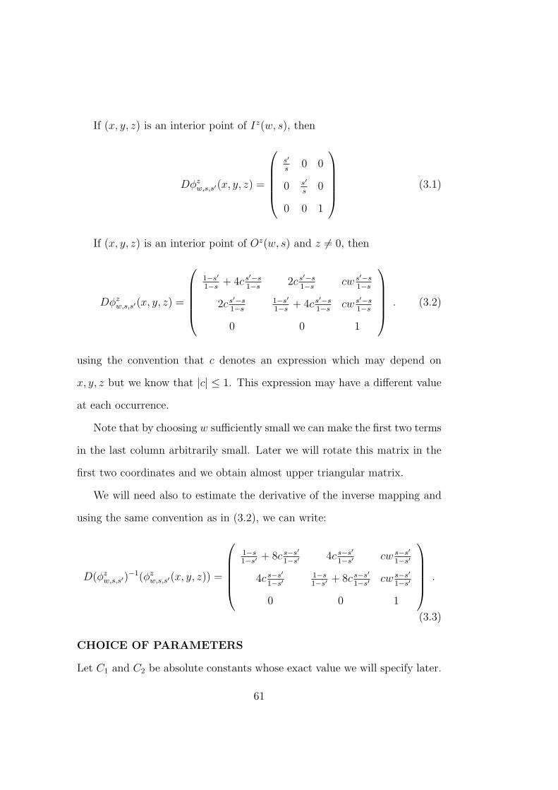
If (x, y, z) is an interior point of Iz(w, s), then
Dφzw,s,s′(x, y, z) =
s′
s0 0
0 s′
s0
0 0 1
(3.1)
If (x, y, z) is an interior point of Oz(w, s) and z 6= 0, then
Dφzw,s,s′(x, y, z) =
1−s′
1−s+ 4c s
′−s1−s
2c s′−s1−s
cw s′−s1−s
2c s′−s1−s
1−s′
1−s+ 4c s
′−s1−s
cw s′−s1−s
0 0 1
. (3.2)
using the convention that c denotes an expression which may depend on
x, y, z but we know that |c| ≤ 1. This expression may have a different value
at each occurrence.
Note that by choosing w sufficiently small we can make the first two terms
in the last column arbitrarily small. Later we will rotate this matrix in the
first two coordinates and we obtain almost upper triangular matrix.
We will need also to estimate the derivative of the inverse mapping and
using the same convention as in (3.2), we can write:
D(φzw,s,s′)
−1(φzw,s,s′(x, y, z)) =
1−s1−s′
+ 8c s−s′
1−s′4c s−s′
1−s′cw s−s′
1−s′
4c s−s′
1−s′1−s1−s′
+ 8c s−s′
1−s′cw s−s′
1−s′
0 0 1
.
(3.3)
CHOICE OF PARAMETERS
Let C1 and C2 be absolute constants whose exact value we will specify later.
61

We can clearly fix t > 1 such that
C1C2
(π2
6
)61
t<
1
2. (3.4)
For k ∈ N, we set
wk =k + 1
tk2 − 1, sk = 1− 1
tk2and s′k = sk
k
k + 1. (3.5)
In this case,
1− s′k1− sk
=tk2 + k
k + 1and
sk − s′k1− sk
wk =tk2 − 1
k + 1wk = 1. (3.6)
It is also easy to check that 0 < sk < 1 and
∞∏
i=1
si > 0.
We will construct a sequence of homeomorphisms Fj which will eventually
converge to f .
CONSTRUCTION OF F1
Let us denote Q0 := Qz(w1). We will construct a sequence of bi-Lipschitz
mappings
fk,1 : Q0onto−→ Q0
and our mapping F1 ∈ W 1,1(Q0,R3) will be later defined as:
F1(x) = limk→∞
fk,1(x).
62

We will also construct a Cantor-type set C1 of positive measure such that
JF1(x) = 0 almost everywhere on C1.
We define f1,1 : Q0onto−→ Q0 by
f1,1(x, y, z) = φzw1,s1,s′1
(x, y, z).
Clearly f1,1 is a bi-Lipschitz homeomorphism. Now each fk,1 will equal to f1,1
on the set Oz(w1, s1) and it remains to define it on R1,1 := Iz(w1, s1). LetQ2,1
be any collection of disjoint, scaled and translated copies of Qz(w2) which
covers f1,1(Iz(w1, s1)) = Iz(w1, s
′1) up to a set of measure zero. That is any
two elements ofQ2,1 have disjoint interiors, and there is a set E2,1 ⊂ Iz(w1, s′1)
of measure 0 such that
Iz(w1, s′1) \ E2,1 ⊂
⋃
Qz∈Q2,1
Qz ⊂ Iz(w1, s′1).
We define f2,1 : Q0 → Q0 by
f2,1(x, y, z) =
φQz
w2,s2,s′2 f1,1(x, y, z) f1,1(x, y, z) ∈ Qz ∈ Q2,1,
f1,1(x, y, z) otherwise.
It is not difficult to check that f2,1 is a bi-Lipschitz homeomorphism. From
now on each fk,1 will equal to f2,1 on
Oz(w1, s1) ∪ f−11,1
(
⋃
Qz∈Q2,1
Os2Qz
)
∪ (f1,1)−1(E2,1)
63
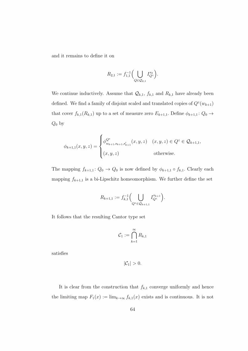
and it remains to define it on
R2,1 := f−11,1
(
⋃
Q∈Q2,1
Is2Qz
)
.
We continue inductively. Assume that Qk,1, fk,1 and Rk,1 have already been
defined. We find a family of disjoint scaled and translated copies of Qz(wk+1)
that cover fk,1(Rk,1) up to a set of measure zero Ek+1,1. Define φk+1,1 : Q0 →
Q0 by
φk+1,1(x, y, z) =
φQz
wk+1,sk+1,s′
k+1(x, y, z) (x, y, z) ∈ Qz ∈ Qk+1,1,
(x, y, z) otherwise.
The mapping fk+1,1 : Q0 → Q0 is now defined by φk+1,1 fk,1. Clearly each
mapping fk+1,1 is a bi-Lipschitz homeomorphism. We further define the set
Rk+1,1 := f−1k,1
(
⋃
Qz∈Qk+1,1
Isk+1
Qz
)
.
It follows that the resulting Cantor type set
C1 :=∞⋂
k=1
Rk,1
satisfies
|C1| > 0.
It is clear from the construction that fk,1 converge uniformly and hence
the limiting map F1(x) := limk→∞ fk,1(x) exists and is continuous. It is not
64

difficult to check that F1 is a one-to-one mapping of Q0 onto Q0. Since Q0
is compact and F1 is continuous we obtain that F1 is a homeomorphism.
WEAK DIFFERENTIABILITY OF F1
Let us estimate the derivative of our functions fm,1. Let us fix m, k ∈ N
such that m ≥ k. If Qz ∈ Qk,1 and (x, y, z) ∈ int(fk,1)−1(I
s′k
Qz), then we
have squeezed our diamond k-times. Using (3.1), (3.5) and the chain rule we
obtain
Dfk,1(x, y, z) =k∏
i=1
ii+1
0 0
0 ii+1
0
0 0 1
=
1k+1
0 0
0 1k+1
0
0 0 1
. (3.7)
Moreover, if (x, y, z) ∈ int(fm,1)−1(O
s′k
Qz), then we have squeezed our diamond
k − 1 times and then we have stretched it once. It follows from (3.1), (3.5),
(3.2), (3.6) and the chain rule that
Dfm,1(x, y, z) =
tk2+kk+1
+ 4c tk2−1
k+12c tk
2−1k+1
c
2c tk2−1
k+1tk2+kk+1
+ 4c tk2−1
k+1c
0 0 1
k−1∏
i=1
ii+1
0 0
0 ii+1
0
0 0 1
=
tk+1k+1
+ 4ck
tk2−1k+1
2ck
tk2−1k+1
c
2ck
tk2−1k+1
tk+1k+1
+ 4ck
tk2−1k+1
c
0 0 1
=: Ak.
(3.8)
It is easy to see that the norm of this matrix can be estimated by Ct.
It is possible to check that fk,1 forms a Cauchy sequence in W 1,1. Since
fk,1 converge to F1 uniformly we obtain that F1 ∈ W 1,1. From (3.7) we obtain
65

that the derivative of fk,1 on Rk,1 and especially on C1 equals to
Dfk,1(x, y, z) =
1k+1
0 0
0 1k+1
0
0 0 1
.
Since Dfk,1 converge to DF1 in L1 we obtain that for almost every (x, y, z) ∈
C1 we have
DF1(x, y, z) =
0 0 0
0 0 0
0 0 1
and therefore JF1(x, y, z) = 0.
Moreover, also f−1k,1 forms a Cauchy sequence in W 1,1
loc and since fk,1
converges uniformly to F1, f−1k,1 converges to F−1
1 uniformly (see Lemma
3.1 [28]). Hence, F1 is a bi–Sobolev mapping.
From now on each Fk will equal to F1 on C1 and we need to define it only
on Q0 \ C1. let us underline that, from the construction,
JF1 6= 0 a.e. on Q0 \ C1.
CONSTRUCTION OF F2 AND F3
As before, we construct a sequence of homeomorphisms
fk,2 : Q0onto−→ Q0
and F2 ∈ W 1,1(Q0,R3) will be later defined as
66

F2(x) = limk→∞
fk,2(x).
We construct a Cantor–type set C2 ⊂ Q0\C1 of positive measure such that
JF2 = 0 a.e. on C2. This time we recover F1(Q0 \ C1) up to a set of measure
zero by a collection of disjoint, scaled, traslated and “rotated ”copies of the
diamond Qy(w1) where
Qy(w) = (x, y, z) ∈ R3 : |x|+ |z| < w(1− |y|).
In Theorem 3.4 and Theorem 3.5, it was essential that all the matrices in-
volved are almost diagonal and thus we can make better estimates of the norm
of their product than simply estimate norm of each matrix. After squeezing
in two directions our mappings are no longer almost diagonal (for example
the matrix from (3.8)) but we repair this using the QR decomposition.
Proposition 3.1. For every n×n matrix A we can find an orthogonal matrix
Q and an upper triangular matrix R such that A = QR.
This linear transformation allows us to make some of the matrices almost
upper triangular which will be sufficient for our estimates.
The mapping F3 is constructed in a similar way using traslated and scaled
copies of Qx(w1) where
Qx(w) = (x, y, z) ∈ R3 : |y|+ |z| < w(1− |x|).
67

CONSTRUCTION OF F4
We will construct a sequence of homeomorphisms f−1k,4 : Q0 → Q0 and our
mapping F4 ∈ W 1,1(Q0,R3) will be later defined as F4(x) = limk→∞ fk,4(x).
So far we have constructed disjoint Cantor type sets such that JF1 = 0 a.e.
on C1, JF2 = 0 a.e. on C2 and JF3 = 0 a.e. on C3. Then, we construct a
Cantor type set C4 of positive measure in the image so that
JF−14
= 0 a.e. on C4
and so that |F−14 (C4)| = 0.
Thus, the sequence of homeomorphisms Fj which will eventually converge
to f is such that
• for j ∈ ⋃k∈N6k + 1, 6k + 2, 6k + 3, JFj= 0 a.e. on Cj with |Cj| > 0
• for j ∈ ⋃
k∈N6k + 4, 6k + 5, 6k + 6, JF−1j
= 0 a.e. on Fj(Cj) and
|Fj(Cj)| > 0.
The mappings F6k+1 and F−16k+4 are squeezing the Cantor type set in the
direction of x and y axes, F6k+2 and F−16k+5 are squeezing after rotation in the
directions x and z and finally F6k+3 and F−16k+6 are squeezing after rotation
in the directions y and z.
PROPERTIES OF f
Now we define f(x) = limj→∞ Fj(x). Since Fj converges uniformly, f is
a homeomorphism. Moreover, DFj and DF−1j is Cauchy in L1 and thus f is
68

bi-Sobolev. Moreover, it results,
∣
∣
∣
∣
∣
∞⋃
j=1
Cj∣
∣
∣
∣
∣
= |Q0|.
This together with JFj= 0 on Cj for each j ∈
⋃
l∈N6l+ 1, 6l+ 2, 6l+ 3
and Fk = Fj on Cj for each k > j, imply that Jf = 0 almost everywhere on
Q0. Analogously we will deduce that Jf−1 = 0 a.e. on Q0.
69

70

Chapter 4
On the continuity of the
Jacobian of orientation
preserving mappings
In several situations it is necessary to integrate the Jacobian. The usual
hypothesis ensuring this integrability has been f ∈ W 1,nloc (Ω,R
n). Here we
are concerned on the minimal condition on the regularity of the map that
ensures the local integrability and the continuity property for the Jacobian
determinant. The right setting will be the Grand Sobolev spaceW1,n)loc (Ω,Rn).
4.1 The integrability of the Jacobian
Let Ω be a domain of Rn and let f = (f 1, . . . , fn) : Ω → Rn be a locally inte-
grable map whose distributional differential Df is locally integrable. Then,
its Jacobian determinant is defined point-wise at almost every point x ∈ Ω.
71

In what follows, in the language of differential forms, we write
Jf (x)dx = df 1 ∧ . . . ∧ dfn(x).
From the Hadamard’s inequality:
|Jf (x)| ≤n∏
i=1
|Df i(x)|, (4.1)
follows that |Jf (x)| ≤ |Df(x)|n and hence, the natural assumption to guar-
antee the integrability of the Jacobian is f ∈ W 1,n.
Without any restriction, there is no reason to expect that the degree
of integrability of Jf is different from that of |Df |n. S. Muller in [73] was
the first to observe that the assumption that Jf does not change sign in Ω,
implies higher integrability of the Jacobian.
A map f is said orientation preserving if Jf ≥ 0 almost everywhere. S.
Muller in [73] proved that, if |Df | ∈ Ln(Ω) and Jf ≥ 0 then Jf ∈ L logL(K)
for any compact set K such that 2K ⊂ Ω. The result can be rephrased as
follows:∫
K
Jf (x) log
(
e+Jf (x)
JK
)
dx ≤ C(K)
∫
Ω
|Df |ndx
where JK is the integral mean of the Jacobian over K.
T. Iwaniec and C. Sbordone in [55] relaxed the natural assumption on
|Df |, proving that if f is an orientation preserving map, that is Jf (x) ≥ 0
a.e., and |Df | ∈ Ln)(Ω), then the Jacobian of f is locally integrable. The
72

key estimate for their proof was the following:
∫
B
Jf (x)dx ≤ c(n) sup0<ε≤1
[
ε
∫
2B
|Df |n−ε
] 1n−ε
for concentric balls B ⊂ 2B ⊂ Ω.
At this point it became clear that the improved integrability property of
the Jacobian could be observed also in spaces slightly larger than W 1,n(Ω).
As a matter of fact, under the hypothesis |Df | ∈ Ln log−1 L(Ω) of G. Moscariello,
([71]), the Jacobian of f is even slightly more integrable; indeed, Jf lies in
L log logLloc(Ω).
A result that interpolate between Muller’s result and [55] is given in [9];
namely, if |Df | ∈ Ln(logL)−s(Ω), 0 ≤ s ≤ 1, then Jf ∈ L(logL)1−s(K) for
any K such that 2K ⊂ Ω, see also L. Greco ([33]).
4.2 The continuity of the Jacobian
Until now we have considered the weakest assumption to guarantee that the
Jacobian determinant is integrable and its integrability properties. A ques-
tion that naturally arises is the following: what are the sharpest hypotheses
under which we may guarantee that if fj ∈ W 1,1(Ω,Rn) converges to f then
Jfj → Jf in some sense? It is well known that if fj f in W 1,n then
Jfj → Jf in the sense of distributions. This is a classical result due to Mor-
rey ([70]) and Reshetnyak ([78]). The key ingredient is that in W 1,n the
point-wise Jacobian agrees with the distributional one. In this setting, in
[55], it was proved that if fj is a sequence of orientation preserving mapping
73

weakly converging to f in W 1,n then,
limj
∫
Ω
ϕJfj =
∫
Ω
ϕJf ∀ϕ ∈ Exp(Ω).
We recall that the exponential class Exp(Ω) is formed by measurable func-
tions u on Ω for which there exists λ = λ(u) > 0 such that
exp(λ|u|) ∈ L1(Ω) .
T. Iwaniec and A. Verde in [60], under the strong convergence in W 1,n of
a sequence fj of orientation preserving mappings, proved that:
‖Jfj − Jf‖L logL(Ω) −→ 0.
Our aim here is to prove a similar result in the case that fj and f are
orientation preserving mappings in the Grand Sobolev space W 1,n)(Ω,Rn)
(see Section 2 for definition). We observe that in this case the distributional
Jacobian is not equal in general to the point-wise one. More precisely,
Theorem 4.1. Let Ω be a bounded domain of Rn. If fj and f are orientation
preserving mappings in W 1,n)(Ω,Rn) such that
fj −→ f in W 1,n)(Ω,Rn)
then
Jfj −→ Jf in L1loc(Ω).
The key tool is the following stability result for the Hodge decomposition,
74

first established in [49],[55] and [57].
Lemma 4.1. For every vector field ω of class Lr(1−ε)(Ω,Rn) with r > 1 and
−∞ < ε < 1− 1r, we can find function η and Du such that
|ω|−εω = η +Du
with u ∈ W 1,r0 (Ω) and divη = 0. This is called a Hodge decomposition and
the following estimates hold:
• If ω = Dv is a gradient field with v ∈ W1,r(1−ε)0 (Ω), then
‖η‖Lr(Ω) ≤ c(n, r)|ε|‖ω‖1−εLr(1−ε) (4.2)
• If ω is divergence free, that is divω = 0, then
‖Du‖Lr(Ω) ≤ c(n, r)|ε|‖ω‖1−εLr(1−ε) (4.3)
From the Hadamard’s inequality (4.1) follows one of the key pointwise
estimate for the Jacobian: for 0 < ε < 1,
|df 1|−ε|Jf (x)dx| ≤(
1 + |df 1|−1)
|Jf (x)dx|
≤|Jf (x)dx|+ |df 2| . . . |dfn| ≤ |Jf (x)dx|+ |Df |n−1.
(4.4)
An important application of the Lp-theory of differential form is:
Proposition 4.1. Let Ω be a bounded domain of Rn, u ∈ W1,n−ε
1−ε
0 (Ω) and
75

g ∈ W 1,n−εn−1 (Ω,Rn−1), then
∫
Ω
du ∧(
dg1 ∧ . . . dgn−1)
= 0 (4.5)
If u ∈ C∞0 (Ω) and g ∈ C∞(Ω,Rn−1) by Stokes’ theorem
∫
Ω
du ∧(
dg1 ∧ . . . dgn−1)
=
∫
Ω
d(
u ∧ dg1 ∧ . . . dgn−1)
=
∫
∂Ω
u ∧(
dg1 ∧ . . . dgn−1)
= 0.
As n−ε1−ε
and n−εn−1
are Holder conjugate then, du ∧ (dg1 ∧ . . . dgn−1) ∈ L1(Ω)
and (4.5) follows via an approximation argument (see [55], page 138).
Proof of Theorem 4.1. It is sufficient to prove the theorem for a subsequence.
Hence, without loss of generality, by assumptions, we can assume that
Dfj(x) → Df(x) a.e. x ∈ Ω. (4.6)
Firstly, we prove the following:
limj→∞
∫
Ω
ϕJfj =
∫
Ω
ϕJf (4.7)
for every nonnegative test functions ϕ ∈ C10(Ω). For technical reason, we
shall consider an auxiliary test function ψ ∈ C10(Ω) which is equal to 1 in the
support of ϕ.
Let fj = (f 1j , . . . , f
nj ). We consider the compactly supported maps:
gj = (ψf 1j , . . . , ψf
n−1j , ϕfn
j ) = (g1j , . . . , gnj ) and g = (ψf 1, . . . , ψfn−1, ϕfn) =
(g1, . . . , gn).
76

Using the calculus of differential forms, the Jacobian determinant of gj
is:
Jgjdx = dg1j ∧ . . . ∧ dgnj =
d(f 1j ) ∧ . . . ∧ d(fn−1
j ) ∧ d(ϕfnj ) on suppϕ
0 otherwise
(4.8)
The telescopic decomposition of the Jacobian ( [53], Section 8) leads to:
(
Jgj − Jg)
dx =(
dg1j ∧ . . . ∧ dgnj)
−(
dg1 ∧ . . . ∧ dgn)
=
=(dg1j − dg1) ∧ dg2j ∧ . . . ∧ dgnj +
+dg1 ∧(
dg2j − dg2)
∧ dg3j ∧ . . . ∧ dgnj + . . .+
+dg1 ∧ . . . ∧ dgn−1 ∧(
dgnj − dgn)
.
(4.9)
Applying the Hodge decomposition to Dgj −Dg, we have:
|Dgj −Dg|−ε(Dgj −Dg) = DGj + Lj (4.10)
with DGj ∈ Ln−ε1−ε , Lj ∈ L
n−ε1−ε and
‖Lj‖n−ε1−ε
≤ c(n, ε)ε‖Dgj −Dg‖1−εn−ε. (4.11)
It is important to realize that Lj becomes small as ε goes to zero.
(4.10) can be rewritten as:
|Dgj −Dg|−ε(Dgkj −Dgk) = DGkj + lkj k = 1, . . . , n (4.12)
where lkj is the 1-form whose coefficients are the entries of the k-th column
77

of Lj.
By (4.9) we have:
|Dgj −Dg|−ε(
Jgj − Jg)
= |Dgj −Dg|−ε
[
(dg1j − dg1) ∧ dg2j ∧ . . . ∧ dgnj +
+ dg1 ∧(
dg2j − dg2)
∧ dg3j ∧ . . . ∧ dgnj + . . .+
+ dg1 ∧ . . . ∧ dgn−1 ∧(
dgnj − dgn)
]
.
(4.13)
We focus our attention on the first term of the previous formula; using
(4.12), we have:
|Dgj −Dg|−ε(dg1j − dg1) ∧ dg2j ∧ . . . ∧ dgnj =
= dG1j ∧ dg2j ∧ . . . ∧ dgnj +l1j ∧ dg2j ∧ . . . ∧ dgnj
(4.14)
Let us estimate both terms in the right hand side of the last formula.
By Proposition 4.1, we find that:
∫
Ω
dG1j ∧ dg2j ∧ . . . ∧ dgnj =
∫
Ω
d(
G1jdg
2j ∧ . . . ∧ dgnj
)
= 0.
Applying Holder inequality and (4.11), we can estimate the second term
78

in (4.14):
∫
Ω
|l1j∧(
dg2j ∧ . . . ∧ dgnj)
| ≤
≤(∫
Ω
|l1j |n−ε1−ε
)1−εn−ε(∫
Ω
|dg2j ∧ . . . ∧ dgnj |n−εn−1
)n−1n−ε
≤c(n, ε)ε‖Dgj −Dg‖1−εn−ε‖Dgj‖n−1
n−ε
≤c(n, ε)‖Dgj −Dg‖1−εLn) ‖Dgj‖n−1
Ln) .
(4.15)
Analogously, we can estimate the k-th term in (4.13) as before, to obtain:
∫
Ω
|Dgj −Dg|−ε|dg1 ∧ . . . ∧ dgk−1 ∧ d(gkj − dgk) ∧ dgk+1j ∧ . . . ∧ dgnj |
≤c(n, ε)ε‖Dgj −Dg‖1−εn−ε‖dg1 ∧ . . . ∧ dgk−1 ∧ dgk+1
j ∧ . . . ∧ dgnj ‖n−εn−1
≤c(n, ε)ε‖Dgj −Dg‖1−εn−ε ‖|Dgk−1| |Dgj|n−k‖n−ε
n−1
≤c(n, ε)‖Dgj −Dg‖1−εLn) ‖Dg‖k−1
Ln) ‖Dgj‖n−kLn)
≤c(n, ε)‖Dgj −Dg‖1−εLn)
(
‖Dg‖n−1Ln) + ‖Dgj‖n−1
Ln)
)
.
79

Thus, for every j we get:
∣
∣
∣
∣
∫
Ω
|Dgj −Dg|−ε(
Jgj − Jg)
dx
∣
∣
∣
∣
≤n c(n, ε)‖Dgj −Dg‖1−εLn)
(
‖Dg‖n−1Ln) + ‖Dgj‖n−1
Ln)
)
.
(4.16)
Using telescopic decomposition of the Jacobian and (4.4), we can pass
to the limit under the integral sign by the dominated convergence theorem.
Since, Dgj converges to Dg in Ln) on the support of ϕ, we have:
lim supj→∞
(∣
∣
∣
∣
∫
suppϕ
(Jgj − Jg)dx
∣
∣
∣
∣
)
= 0. (4.17)
By (4.8), (4.17) is equivalent to:
lim supj→∞
(∣
∣
∣
∣
∫
suppϕ
ϕJfj − ϕJf
+
∫
suppϕ
fnj (df
1j ∧ . . . ∧ dfn−1
j ∧ dϕ)− fn(df 1 ∧ . . . ∧ dfn−1 ∧ dϕ)∣
∣
∣
∣
)
= 0.
Now, we can apply the imbedding of Grand Sobolev space W 1,n) into
Exp(Ω) (see [27]). It means that fnj , f
n belong to Lp for every 1 < p <∞ and
by assumptions it follows that fnj converges to fn in Lp for every 1 < p <∞.
This remark together with the telescopic decomposition of the Jacobian and
80

Holder’s inequality gives:
lim supj→∞
(∣
∣
∣
∣
∫
suppϕ
fnj (df
1j ∧ . . . ∧ dfn−1
j ∧ dϕ)− fn(df 1 ∧ . . . ∧ dfn−1 ∧ dϕ)∣
∣
∣
∣
)
= lim supj→∞
(∣
∣
∣
∣
∫
suppϕ
(fnj − fn)(df 1
j ∧ . . . ∧ dfn−1j ∧ dϕ)
+
∫
suppϕ
fn(df 1j ∧ . . . ∧ dfn−1
j − df 1 ∧ . . . ∧ dfn−1) ∧ dϕ)∣
∣
∣
∣
)
= 0.
(4.18)
Therefore,
lim supj→+∞
(∣
∣
∣
∣
∫
suppϕ
ϕJfj − ϕJf
∣
∣
∣
∣
)
= 0.
Since fj and f are orientation preserving maps, we get:
limj→+∞
∫
suppϕ
ϕJfj =
∫
suppϕ
ϕJf . (4.19)
for every non negative ϕ ∈ C10(Ω).
Now, we are in position to prove the thesis.
We recall, by a Theorem of Iwaniec and Sbordone ([55]), that Jfj and Jf
belong to L1loc(Ω). On the other hand, by assumptions, Jfj converges to Jf
a.e. Hence, an application of Fatou’s Lemma gives, for every measurable set
E ⊂⊂ Ω:
∫
E
Jf ≤ lim infj→+∞
∫
E
Jfj ≤ lim supj→+∞
∫
E
Jfj
≤ limj→+∞
∫
E
ϕJfj
=
∫
E
ϕJf
81
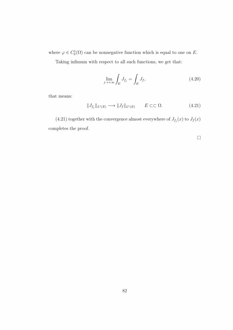
where ϕ ∈ C10(Ω) can be nonnegative function which is equal to one on E.
Taking infimum with respect to all such functions, we get that:
limj→+∞
∫
E
Jfj =
∫
E
Jf , (4.20)
that means:
‖Jfj‖L1(E) −→ ‖Jf‖L1(E) E ⊂⊂ Ω. (4.21)
(4.21) together with the convergence almost everywhere of Jfj(x) to Jf (x)
completes the proof.
82

Bibliography
[1] L. Ambrosio, N. Fusco, D. Pallara: Functions of bounded variation and
free discontinuity problems, Oxford Mathematical Monographs, The
Clarendon Press, Oxford University Press, New York, (2000).
[2] K. Astala,T. Iwaniec, P. Koskela, and G. Martin: Mappings of BMO-
bounded distortion, Math. Ann. 317 (2000), 703–726.
[3] K. Astala, T. Iwaniec, G. Martin. Elliptic Partial Differential Equations
and Quasiconformal Mappings in the Plane, Princeton Mathematical
Series vol. 24, (2008).
[4] S. Antman, Fundamental mathematical problems in the theory of non-
linear elasticity. Numerical solution of partial differential equations, III
(Proc. Third Sympos. (SYNSPADE), Univ. Maryland, College Park,
Md., 1975), pp. 35–54. Academic Press, New York, 1976.
[5] J. Ball, Convexity conditions and existence theorems in nonlinear elas-
ticity, Arch. Rational Mech. Anal. 63 (1976/77), no. 4, 337–403.
[6] L. Bers, L. Nirenberg: On linear and nonlinear elliptic boundary value
problems in the plane, Convegno Internazionale sulle Equazioni Lineari
83

alle Derivate Parziali, Trieste, 1954, Edizioni Cremonese, Roma, 1955,
141– 167.
[7] B. Bojarski: Generalized solutions of systems differential equations
of first order and of elliptic type with discontinuous coefficients, Math.
Sb. (N.S.) 43 (85) (1957), 451– 503.
[8] B. Bojarski and T.Iwaniec: Analytical foundations of the theory of
quasiconformal mappings in Rn. Ann. Acad. Sci. Fenn. Ser. A I Math.
8 (1983), 257–324.
[9] H. Brezis, N. Fusco and C.Sbordone, Integrability for the Jacobian
of orientation preserving mappings, J. Funct. Anal. 115 (1993), no. 2,
425–431.
[10] H. Brezis and H. Nguyen, The Jacobian determinant revisited, Invent.
Math. 185 (2011), no. 1, 17–54.
[11] R. Caccioppoli: Fondamenti per una teoria generale delle funzioni
pseudoanalitiche di una variabile complessa , Rend. Accad. Naz. Lincei
13 (1952), 197–204.
[12] R. Cerny, Homeomorphism with zero Jacobian: Sharp integrability of
the derivative, J. Math. Anal. Appl, 373, (2011), 161–174.
[13] L. Cesari: Sulle trasformazioni continue. Ann. Mat. Pura Appl. (4)
21, (1942), 157–188.
84

[14] P. Ciarlet, Mathematical elasticity. Vol. II. Theory of plates. Studies in
Mathematics and its Applications, 27. North-Holland Publishing Co.,
Amsterdam, 1997.
[15] M. Csornyei, S. Hencl, J. Maly: Homeomorphisms in the Sobolev space
W 1,n−1. J. Reine Angew. Math. 644 (2010), 221-235.
[16] S. Daneri and A. Pratelli, Smooth approximation of bi–
Lipschitz orientation–preserving homeomorphisms, preprint (2011),
arXiv:1106.1192.
[17] G. David: Solution de l’equation de Beltrami avec ‖µ‖∞ = 1, Ann.
Acd. Sci. Fenn. Ser. A I Math. 13:1 (1988), 25-70.
[18] P. Di Gironimo, L. D’Onofrio, C. Sbordone, R. Schiattarella:
Anisotropic Sobolev homeomorphisms, Ann. Acad. Sci. Fenn. Math.,
36, (2011), 593–602.
[19] L. D’Onofrio, S. Hencl and R. Schiattarella, Bi-Sobolev homeomor-
phism with zero Jacobian almost everywhere, Preprint MATH-KMA-
2012/408.
[20] L. D’Onofrio, C. Sbordone and R. Schiattarella, The Grand Sobolev
homeomorphisms and their measurability properties, Advanced Nonlin-
ear Studies, 12 (2012), no. 4, 767–782.
[21] L. D’Onofrio and R. Schiattarella, On the continuity of Jacobian of
orientation preserving mappings in the Grand Sobolev space, preprint.
85

[22] L. D’Onofrio and R. Schiattarella, On the total variations for the
inverse of a BV-homeomorphism, to appear in Adv. Calc.Var, DOI
10.1515/acv-2012-0103.
[23] D. Edmunds, P. Gurka and B. Opic, On embeddings of logarithmic
Bessel potential spaces, J. Funct. Anal. 146 (1997), no. 1, 116–150.
[24] F. Farroni, R. Giova, G. Moscariello and R. Schiattarella: Homeomor-
phisms of finite inner distortion: composition operators on Zygmund-
Sobolev and Lorentz–Sobolev spaces, preprint 2012.
[25] H. Federer: Geometric Measure Theory, Die Grundlehren der math-
ematischen Wissenschaften, Band 153 Springer - Verlag, New York
(1969) (Second edition 1996).
[26] I. Fonseca, G. Leoni and J. Maly, Weak continuity and lower semicon-
tinuity results for determinants, Arch. Ration. Mech. Anal. 178 (2005),
no. 3, 411–448.
[27] N. Fusco, P. Lions and C. Sbordone, Sobolev imbedding theorems in
borderline cases, Proc. Amer. Math. Soc. 124 (1996), no. 2, 561–565.
[28] N. Fusco, G. Moscariello, C. Sbordone: The limit of W 1,1-
homeomorphisms with finite distortion, Calc. Var. 33 (2008), 377-390.
[29] F. W. Gehring and O. Lehto: On the total differentiability of functions
of a complex variable, Ann. Acad. Sci. Fenn. Ser. A I 272, (1959), 1–9.
86

[30] F. Giannetti, L. Greco and A. Passarelli di Napoli: Regularity of map-
pings of finite distortion, Funct. Approx. Comment. Math. 40 (2009),
no. 1, 91–103.
[31] F. Giannetti, T. Iwaniec, J. Onninen and A. Verde: Estimates of Ja-
cobians by subdeterminants, J. Geom. Anal. 12 (2002), no. 2, 223–254.
[32] M. Giaquinta, G. Modica and J. Soucek: Area and the area formula.
Proceedings of the Second International Conference on Partial Differ-
ential Equations (Italian) (Milan, 1992). Rend. Sem. Mat. Fis. Milano
62 (1992), 53-87 (1994).
[33] L. Greco, A remark on the equality det Df = Det Df, Differential Inte-
gral Equations 6 (1993), 1089–1100.
[34] L. Greco, T. Iwaniec, G. Moscariello: Limits of the improved integra-
bility of the volume forms, Indiana Univ. Math. J. 44 (1995), 305-339.
[35] L. Greco, C. Sbordone and R. Schiattarella, Composition of bi-Sobolev
homeomorphisms, Proc. Roy. Soc. Edinburgh Sect. A 142 (2012), no.
1, 61–80.
[36] L. Greco, C. Sbordone, C. Trombetti: A note on planar homeomor-
phisms, Rend. Accad. Sci. Fis. Mat. Napoli (4) 75 (2008), 53-59.
[37] L. Greco and A. Verde, On some nonlinear expressions of the Jacobian.
Diff. Int. Eq. 13 (2000), no. 10-12, 1569–1582.
[38] S. Hencl: On the weak differentiability of u f−1, to appear in Math.
Scand. 107 (2010), no. 2, 198–208.
87

[39] S. Hencl: Sharpness of the assumptions for the regularity of a home-
omorphism, Michigan Math. J. 59 (2010), no. 3, 667–678.
[40] S. Hencl: Sobolev homeomorphism with zero Jacobian almost every-
where, J. Math. Pures Appl. (9) 95 (2011), no. 4, 444-458.
[41] S. Hencl, P. Koskela: Lectures on Mappings of finite distortion, Mono-
graph, (2012), preprint.
[42] S. Hencl, P. Koskela: Mappings of finite distortion: composition oper-
ator, Ann. Acd. Sci. Fenn. Math. 33 (2008), 65-80.
[43] S. Hencl, P. Koskela: Regularity of the inverse of a planar Sobolev
homeomorphism, Arch. Ration. Mech. Anal. 180 (2006), 75-95.
[44] S. Hencl, P. Koskela and J. Maly: Regularity of the inverse of a Sobolev
homeomorphism in space, Proc. Roy. Soc. Edinburgh Sect. A 136:6
(2006), 1267-1285.
[45] S. Hencl, P. Koskela and J. Onninen: Homeomorphisms of Bounded
Variation, Arch. Ration. Mech. Anal. 186, 2007, 351-360.
[46] S. Hencl, P. Koskela and X. Zhong, Mappings of finite distortion: re-
verse inequalities for the Jacobian. J. Geom. Anal. 17 (2007), no. 2,
253–273.
[47] S. Hencl, J. Maly: Jacobians of Sobolev homeomorphisms, Calc. Var.
Partial Differential Equations 38 (2010), no. 1–2, 233–242.
88

[48] S. Hencl, G. Moscariello, A. Passarelli di Napoli and C. Sbordone: Bi-
Sobolev mappings and elliptic equations in the plane, J. Math. Anal.
Appl. 355 (2009), 22-32.
[49] T. Iwaniec : p -harmonic tensors and quasiregular mappings. Ann. of
Math. (2) 136 (1992), no. 3, 589–624.
[50] T. Iwaniec, P. Koskela and G. Martin: Mappings of BMO-distortion
and Beltrami-type operators. Dedicated to the memory of Tom Wolff.
J. Anal. Math. 88 (2002), 337-381.
[51] T. Iwaniec, P. Koskela, G. Martin and C. Sbordone, Mappings of finite
distortion: Ln logγ L -integrability, J. London Math. Soc. (2) 67 (2003),
no. 1, 123–136.
[52] T. Iwaniec, L. Kovalev and J. Onninen Diffeomorphic approximation of
Sobolev homeomorphisms, Arch. Ration. Mech. Anal. 201 (2011), no.
3, 1047–1067.
[53] T. Iwaniec and G. Martin, Geometric function theory and non-linear
analysis, Oxford Mathematical Monographs. The Clarendon Press, Ox-
ford University Press, New York, 2001.
[54] T. Iwaniec, J. Onninen: Deformations of finite conformal energy:
Boundary behavior and limit theorems., Trans. Amer. Math. Soc. 363
(2011), no. 11, 5605–5648.
89

[55] T. Iwaniec and C. Sbordone, On the integrability of the Jacobian under
minimal hypotheses, Arch. Rational Mech. Anal. 119 (1992), no. 2, 129–
143.
[56] T. Iwaniec and C. Sbordone, Quasiharmonic fields, Ann. Inst. H.
Poincare Anal. Non Lineaire 18 (2001), no. 5, 519–572.
[57] T. Iwaniec and C. Sbordone, Weak minima of variational integrals, J.
Reine Angew. Math. 454 (1994), 143–161.
[58] T. Iwaniec and V. Sverak: On mappings with integrable dilatation.
Proc. Amer. Math. Soc. 118 (1993), 181–188.
[59] T. Iwaniec and V. Sverak: On mappings with integrable dilatation.
Proc. Amer. Math. Soc. 118 (1993), 181–188.
[60] T. Iwaniec and A. Verde: On the Operator L(f) = f log |f |, Journ. of
Funct Anal. 169 (1999) 391–420.
[61] J. Kauhanen, P. Koskela and J. Maly: On functions with derivatives
in a Lorentz space, Manuscripta Math. 100 (1999), 87-101.
[62] J. Kauhanen, P. Koskela and J. Maly: Mappings of finite distortion:
condition N, Michigan Math. J. 49 (2001), 169-181.
[63] P. Koskela and J. Maly: Mappings of finite distortion: the zero set of
the Jacobian, J. Eur. Math. Soc. 5:2 (2003), 95-105.
[64] P. Koskela and J. Onninen: Mappings of finite distortion: decay of the
Jacobian in the plane, Adv. Calc. Var. 1 (2008), 3, 309-321.
90

[65] O. Lehto, K. Virtanen: Quasiconformal Mappings in the Plane,
Springer- Verlag, Berlin, (1971).
[66] J. Maly: Lectures on change of variables in integral, Graduate School
in Helsinki, (2001).
[67] M. Marcus and V. Mizel: Transformations by functions in Sobolev
spaces and lower semicontinuity for parametric variational problems,
Bull. Amer. Math. Soc. 79 (1973), 790–795.
[68] O. Martio and W. Ziemer: Lusin’s condition (N) and mappings with
nonnegative Jacobians, Michigan Math. J. 39 (1992), no. 3, 495–508.
[69] C.B. Morrey: On the solutions of quasi-linear elliptic partial differen-
tial equations, Trans. Amer. Math. Soc. 43 (1938) 126–166.
[70] C. B. Morrey, Multiple integrals in the calculus of variations, Springer
Verlag, New York, 1966.
[71] G. Moscariello, On the integrability of the Jacobian in Orlicz spaces,
Math. Japon. 40 (1994), no. 2, 323–329.
[72] G. Moscariello and A. Passarelli di Napoli, The regularity of the in-
verses of Sobolev homeomorphisms with finite distortion,to appear on
J. Geom. Anal..
[73] S. Muller, Higher integrability of determinants and weak convergence
in L1, J. Reine Angew. Math. 412 (1990), 20–34.
[74] J. Onninen: Regularity of the inverse of spatial mappings with finite
distortion, Calc. Var. 26 (3) (2006), 331-341.
91

[75] S. P. Ponomarev: An example of an ACTLp homeomorphism that is
not absolutely continuous in the sense of Banach. Dokl. Akad. Nauk
SSSR 201 (1971), 1053–1054.
[76] S. P. Ponomarev: Property N of homeomorphism in the class W 1,p,
Transl. Sibirskii Math., 28 (2) (1987), 140-148.
[77] Yu. G. Reshetnyak: Some geometrical properties of functions and map-
pings with generalized derivatives, Sibirsk. Math. Zh. 7 (1966), 886-919.
[78] Y. G. Reshetnyak, Stability theorems for mappings with bounded excur-
sion, Sib. Math. J. 9 (1968), 499–512.
[79] V. Ryazanov, U. Srebro and E. Yakubov: Finite mean oscillation and
the Beltrami equation, Israel J. Math. 153 (2006), 247-266.
[80] R. Schiattarella: Composition of bisobolev mappings, Rend. Accad. Sci.
Fis. Mat. Napoli (4) 77 (2010), 7–14.
[81] J. Vaisala: Two new characterizations for quasiconformality, Ann.
Acad. Sci. Fenn. Ser. A I Math., 362, (1965), 1-12.
[82] S. K. Vodop’janov and V. M. Gol’dsteın: Quasiconformal mappings,
and spaces of functions with first generalized derivatives. (Russian)
Sibirsk. Mat. Z. 17 (1976), no. 3, 515-531.
[83] W.P. Ziemer: Change of variables for absolutely continuous functions,
Duke Math. J. ,36:1, (1969), 171–178.
92