
Enrico Schiattarella - polito.it · enrico _dot_ schiattarella _at_ gmail _dot_ com Thanks! ... In...
133
POLITECNICO DI TORINO SCUOLA DI DOTTORATO Dottorato in Ingegneria Elettronica e delle Comunicazioni - XVIII Ciclo Tesi di Dottorato High-Performance Packet Switching Architectures Enrico Schiattarella Tutore: Prof. Fabio Neri Coordinatore del corso di dottorato: Prof. Ivo Montrosset Marzo 2006
-
Upload
nguyenmien -
Category
Documents
-
view
222 -
download
0
Transcript of Enrico Schiattarella - polito.it · enrico _dot_ schiattarella _at_ gmail _dot_ com Thanks! ... In...

POLITECNICO DI TORINO
SCUOLA DI DOTTORATODottorato in Ingegneria Elettronica e delle Comunicazioni- XVIII Ciclo
Tesi di Dottorato
High-Performance Packet SwitchingArchitectures
Enrico Schiattarella
Tutore:Prof. Fabio Neri
Coordinatore del corso di dottorato:Prof. Ivo Montrosset
Marzo 2006

This work is Copyright 2006 (c) Enrico Schiattarella.
You are free to use and redistribute this work for personal andeducational purposes.
The author kindly asks to be informed about any usage of this work.
Please direct questions, requests and comments to:
enrico _dot_ schiattarella _at_ gmail _dot_ com
Thanks!

Abstract
Packet switches are at the heart of modern communication networks. Initially de-ployed for local- and wide-area computer networking, they are now being used in differ-ent contexts, such as interconnection networks for High-Performance Computing (HPC),Storage Area Networks (SANs) and Systems-on-Chip (SoC) communication. Each appli-cation domain, however, has peculiar requirements in termsof bandwidth, latency, scal-ability and delivery guarantee. These requirements must becarefully taken into accountand have a major impact on the design of the switch.
In this thesis we present two novel switching architectures, aimed at shared-memorysupercomputing and storage networking respectively. We describe the general architec-ture of the two systems and discuss how specific requirementsand current technologytrends have impacted the design. More important, we presentsome architectural inno-vations that address important issues concerning performance and scalability of input-queued switches.
In particular, we propose techniques that enable the construction of distributed (multi-chip) schedulers for large crossbars, develop a scheme for integrated scheduling of unicastand multicast traffic and study flow-control mechanisms thatallow switches to achievelossless behavior while providing fine-grained control of active flows. Simulation is usedto understand the impact of the proposed solutions and evaluate system performance.

Table of contents
Acknowledgments V
1 Introduction 11.1 Background . . . . . . . . . . . . . . . . . . . . . . . . . . . . . . . . . 11.2 Contributions . . . . . . . . . . . . . . . . . . . . . . . . . . . . . . . . 21.3 Outline of the Thesis . . . . . . . . . . . . . . . . . . . . . . . . . . . . 3
2 Packet Switching Basics 52.1 Definitions . . . . . . . . . . . . . . . . . . . . . . . . . . . . . . . . . . 52.2 General Architecture of a Packet Switch . . . . . . . . . . . . . .. . . . 62.3 Switching Fabric . . . . . . . . . . . . . . . . . . . . . . . . . . . . . . 7
2.3.1 Fabric properties . . . . . . . . . . . . . . . . . . . . . . . . . . 72.3.2 Crossbar . . . . . . . . . . . . . . . . . . . . . . . . . . . . . . 8
2.4 Buffering Strategies . . . . . . . . . . . . . . . . . . . . . . . . . . . . .92.4.1 Output-queued (OQ) . . . . . . . . . . . . . . . . . . . . . . . . 92.4.2 Input-queued (IQ) . . . . . . . . . . . . . . . . . . . . . . . . . 102.4.3 IQ switches with Virtual Output Queueing (VOQ) . . . . . .. . 112.4.4 Combined Input-Output-Queued (CIOQ) Switches . . . . .. . . 13
2.5 Scheduling Unicast Traffic in IQ Switches . . . . . . . . . . . . .. . . . 132.5.1 Optimal Scheduling Algorithm . . . . . . . . . . . . . . . . . . . 132.5.2 Parallel Iterative Matching Algorithms . . . . . . . . . . .. . . . 142.5.3 Sequential Matching Algorithms . . . . . . . . . . . . . . . . . .17
2.6 Scheduling Multicast Traffic in IQ Switches . . . . . . . . . . .. . . . . 182.6.1 Definitions . . . . . . . . . . . . . . . . . . . . . . . . . . . . . 182.6.2 Queueing . . . . . . . . . . . . . . . . . . . . . . . . . . . . . . 192.6.3 Scheduling . . . . . . . . . . . . . . . . . . . . . . . . . . . . . 19
I A Switching Architecture for Shared-Memory Supercomputers 21
3 Supercomputers and Interconnection Networks 22
3.1 Supercomputing Systems . . . . . . . . . . . . . . . . . . . . . . . . . . 223.1.1 Shared-Memory vs. Message-Passing . . . . . . . . . . . . . . .233.1.2 UMA vs. NUMA . . . . . . . . . . . . . . . . . . . . . . . . . . 233.1.3 Custom vs. Off-the-shelf . . . . . . . . . . . . . . . . . . . . . . 25
3.2 Interconnection Networks . . . . . . . . . . . . . . . . . . . . . . . . .. 263.2.1 Direct networks . . . . . . . . . . . . . . . . . . . . . . . . . . . 273.2.2 Indirect networks and MINs . . . . . . . . . . . . . . . . . . . . 28
4 The OSMOSIS Project 314.1 Electronics and optics in packet switching . . . . . . . . . . .. . . . . . 31
4.1.1 Electronic switching . . . . . . . . . . . . . . . . . . . . . . . . 314.1.2 Optical devices . . . . . . . . . . . . . . . . . . . . . . . . . . . 324.1.3 Optical switching architectures . . . . . . . . . . . . . . . . .. . 32
4.2 The OSMOSIS System . . . . . . . . . . . . . . . . . . . . . . . . . . . 334.2.1 Goals and requirements . . . . . . . . . . . . . . . . . . . . . . . 334.2.2 System Overview . . . . . . . . . . . . . . . . . . . . . . . . . . 344.2.3 Data path . . . . . . . . . . . . . . . . . . . . . . . . . . . . . . 354.2.4 Control path . . . . . . . . . . . . . . . . . . . . . . . . . . . . 354.2.5 Multistage scalability . . . . . . . . . . . . . . . . . . . . . . . . 37
5 Distributed Implementation of Crossbar Schedulers 395.1 Iterative Matching Algorithms . . . . . . . . . . . . . . . . . . . . .. . 39
5.1.1 Two- vs. three-phase algorithms . . . . . . . . . . . . . . . . . .405.1.2 Sizing experiments . . . . . . . . . . . . . . . . . . . . . . . . . 41
5.2 Distribution Challenges . . . . . . . . . . . . . . . . . . . . . . . . . .. 425.2.1 Monolithic DRRM implementation . . . . . . . . . . . . . . . . 435.2.2 Separating Input Selectors from Output Selectors . . .. . . . . . 445.2.3 Achieving further distribution levels . . . . . . . . . . . .. . . . 45
5.3 Distributed Implementation . . . . . . . . . . . . . . . . . . . . . . .. . 465.3.1 Pointer Update Approaches . . . . . . . . . . . . . . . . . . . . 465.3.2 Pending Request Counters . . . . . . . . . . . . . . . . . . . . . 48
5.4 Performing Multiple Iterations . . . . . . . . . . . . . . . . . . . .. . . 495.5 Simulation Results . . . . . . . . . . . . . . . . . . . . . . . . . . . . . 51
5.5.1 Uniform Bernoulli Traffic . . . . . . . . . . . . . . . . . . . . . 515.5.2 Bursty and Nonuniform Traffic . . . . . . . . . . . . . . . . . . . 54
6 Fair Integrated Scheduling of Unicast and Multicast Traffic in Input-QueuedSwitches 566.1 Motivation . . . . . . . . . . . . . . . . . . . . . . . . . . . . . . . . . . 566.2 Fair Integrated Scheduling . . . . . . . . . . . . . . . . . . . . . . . .. 58
6.2.1 Reference architecture . . . . . . . . . . . . . . . . . . . . . . . 58

6.2.2 Achieving fairness . . . . . . . . . . . . . . . . . . . . . . . . . 596.2.3 Integration policy . . . . . . . . . . . . . . . . . . . . . . . . . . 606.2.4 Remainder-service policy . . . . . . . . . . . . . . . . . . . . . 60
6.3 Simulation Results . . . . . . . . . . . . . . . . . . . . . . . . . . . . . 616.4 Enhanced Remainder-Service Policy . . . . . . . . . . . . . . . . .. . . 626.5 Implementation Complexity . . . . . . . . . . . . . . . . . . . . . . . .64
6.5.1 Integration policy . . . . . . . . . . . . . . . . . . . . . . . . . . 656.5.2 Base remainder-service policy . . . . . . . . . . . . . . . . . . .656.5.3 Enhanced remainder-service policy . . . . . . . . . . . . . . .. 65
7 Conclusions – Part I 67
II A Switching Architecture for Storage Area Networks 69
8 Introduction to Storage Area Networks 708.1 Limits of directly-attached storage . . . . . . . . . . . . . . . .. . . . . 708.2 Storage Area Networks . . . . . . . . . . . . . . . . . . . . . . . . . . . 718.3 Networking Technologies for SANs . . . . . . . . . . . . . . . . . . .. 73
8.3.1 Fibre Channel . . . . . . . . . . . . . . . . . . . . . . . . . . . . 748.3.2 Credit-based flow control . . . . . . . . . . . . . . . . . . . . . . 74
9 The Switching Architecture 769.1 System Overview . . . . . . . . . . . . . . . . . . . . . . . . . . . . . . 769.2 Data Path . . . . . . . . . . . . . . . . . . . . . . . . . . . . . . . . . . 78
9.2.1 Linecards . . . . . . . . . . . . . . . . . . . . . . . . . . . . . . 789.2.2 Switching fabric . . . . . . . . . . . . . . . . . . . . . . . . . . 79
9.3 Control Path . . . . . . . . . . . . . . . . . . . . . . . . . . . . . . . . . 809.3.1 Internal flow-control . . . . . . . . . . . . . . . . . . . . . . . . 809.3.2 The central arbiter . . . . . . . . . . . . . . . . . . . . . . . . . 82
9.4 Extension to Support Multicast Traffic . . . . . . . . . . . . . . .. . . . 829.4.1 Linecards . . . . . . . . . . . . . . . . . . . . . . . . . . . . . . 839.4.2 Switching fabric . . . . . . . . . . . . . . . . . . . . . . . . . . 839.4.3 Central arbiter . . . . . . . . . . . . . . . . . . . . . . . . . . . 84
10 Performance Under Unicast Traffic 8510.1 Simulation model . . . . . . . . . . . . . . . . . . . . . . . . . . . . . . 8510.2 Simulation settings . . . . . . . . . . . . . . . . . . . . . . . . . . . . .8510.3 Traffic model . . . . . . . . . . . . . . . . . . . . . . . . . . . . . . . . 8610.4 Diagonal traffic . . . . . . . . . . . . . . . . . . . . . . . . . . . . . . . 87
10.4.1 Small packets . . . . . . . . . . . . . . . . . . . . . . . . . . . . 89
10.4.2 Large packets . . . . . . . . . . . . . . . . . . . . . . . . . . . . 8910.4.3 Variable-size packets . . . . . . . . . . . . . . . . . . . . . . . . 89
10.5 Uniform traffic . . . . . . . . . . . . . . . . . . . . . . . . . . . . . . . 9010.5.1 The effects of internal flow-control . . . . . . . . . . . . . .. . 9110.5.2 Small packets . . . . . . . . . . . . . . . . . . . . . . . . . . . . 9210.5.3 Large packets . . . . . . . . . . . . . . . . . . . . . . . . . . . . 9210.5.4 Variable-size packets . . . . . . . . . . . . . . . . . . . . . . . . 93
10.6 Improving system performance . . . . . . . . . . . . . . . . . . . . .. . 9410.6.1 Increased internal speed-up in the switching fabric. . . . . . . . 9410.6.2 Extended memory size in the switching fabric . . . . . . .. . . . 9510.6.3 Link speed-up between the switching fabric and the linecards . . 96
10.7 Linear traffic . . . . . . . . . . . . . . . . . . . . . . . . . . . . . . . . 98
11 Performance Under Multicast Traffic 10011.1 Simulation Model . . . . . . . . . . . . . . . . . . . . . . . . . . . . . . 10011.2 Simulation settings . . . . . . . . . . . . . . . . . . . . . . . . . . . . .10111.3 Traffic model . . . . . . . . . . . . . . . . . . . . . . . . . . . . . . . . 10111.4 Broadcast traffic scenario - One active port per linecard . . . . . . . . . . 10311.5 Broadcast scenario - Four active ports on each linecard. . . . . . . . . . 10411.6 “Residue” traffic pattern . . . . . . . . . . . . . . . . . . . . . . . . .. 106
11.6.1 “Residue 2” traffic pattern . . . . . . . . . . . . . . . . . . . . . 10711.6.2 Modified “residue” traffic pattern with fanout 2 . . . . .. . . . . 11111.6.3 “Residue 3” traffic pattern . . . . . . . . . . . . . . . . . . . . . 112
11.7 Uniform traffic pattern . . . . . . . . . . . . . . . . . . . . . . . . . . .114
12 Conclusions – Part II 116
Bibliography 118

Acknowledgments
Despite the numerous challenges and the many difficulties found along the way, my years
as a Ph.D. student at Politecnico di Torino have really flown by.
The Telecommunication Networks Group has been an excellentenvironment to under-
take doctoral studies. I am sincerely grateful to professors Marco Ajmone Marsan and
Fabio Neri for attracting so many talented individuals overthe years and forming such
a brilliant research group. I wish to thank personally the people I have closely worked
with and who have had a major role in my education as a researcher: professors Emilio
Leonardi, Andrea Bianco and Paolo Giaccone. My gratitude also goes to all the other
members of the group, including fellow students, for being friendly, helpful and creating
such a lively and entertaining environment. A special thankto prof. Monica Visintin, for
her gentle attitude, dedication and encouraging words.
A significant part of my work has been performed at external research institutions.
I wish to thank Ronald Luijten of the IBM Zurich Research Lab,for giving me the op-
porunity to visit his group for more than one year, Dr. CyrielMinkenberg, for his precious
mentoring, and all the other members of the group, for being relentless sources of inspi-
ration and enthusiasm. Thanks also to Dr. Francesco Masetti-Placci, for allowing me to
spend a summer at Alcatel R&I, in beautiful Paris.
I gratefully acknowledge prof. Andrzej Jajszczyk of the AGHUniversity of Science
and Technology and prof. Angelos Bilas of the University of Crete, who kindly accepted
to review the entire manuscript.
Finally, a whole-hearted thank to my family. Your trust madethis possible.

Chapter 1
Introduction
1.1 Background
The history of packet-switched networks dates back to the ’60s, when deployment ofthe ARPANET, ancestor of the Internet, was initiated. In the’90s the Internet becamea global and ubiquitous networking infrastructure, used for business, entertainment andscientific purposes. Since then, the bandwidth demand of theInternet community hasbeen steadily increasing at exponential rates. To satisfy it, researchers and engineers havestudied extensively the design of high-performance switching fabrics, that are at the heartof Internet routers. Today’s commercial Internet routers offer aggregate bandwidths onthe order of terabits per second and employ sophisticated algorithms for packet buffering,processing and scheduling.
The success of this technology has led researchers to investigate its usage in otherdomains, where the communication subsystem has become a primary performance bot-tleneck. Packet switching is being used to build interconnection networks for High-Performance Computing (HPC) systems, where a large number of computing nodes andmemory banks must be interconnected. It is replacing the traditional bus-based inter-connection between servers and storage devices, giving birth to Storage Area Networks(SANs). More recently, it is also being used for Systems-on-Chip (SoC) interconnects.
While the benefits of using packet switching in these domainshave long been recog-nized, it is important to remember that each of them has its specific set of requirements,significantly different from those typical of computer networks. Table 1.1 summarizes therequirements for packet switches used in computer networksas well as in the two otherdomains we are considering. The most significant differences are in terms of latency,aggregate bandwidth and delivery guarantee.
Moreover, current technology trends are playing a significant role in the design ofpacket switches. Issues such as power consumption, chip I/Obandwidth limitations andpackaging constraints are becoming primary concerns for designers.
1

1 – Introduction
IP Routers Fibre Channel HPC InterconnectsSAN Switches
Throughput Very Important Very Important Moderately ImportantLatency Not Important Moderately Important Very ImportantDelivery Can Tolerate Losses not Losses notGuarantee Small Losses Acceptable AcceptableLine Rate/ < 10 Gb/s < 10 Gb/s ≥ 40 Gb/sPort Count ∼ 100 ports ∼ 100 ports ∼ 1000 ports
Table 1.1. Requirements of domain-specific interconnection networks.
Domain−specific
Requirements
Trends
Technology
Architectural
Innovations
Switching Architectures
ATM Switches
IP Routers and
Research on
Figure 1.1. Contributions and context of the thesis.
1.2 Contributions
In this thesis we present two novel switching architectures, aimed at HPC interconnectsand Storage Area Networks respectively. We discuss how the specific requirements ofthe respective domains and current technology trends have influenced the design. Moreimportantly, we present some of the architectural innovations that allow them to satisfythe demanding needs of their operating environments. The contributions and the contextof this work are illustrated in Figure 1.1.
Work described in Part I was performed in the context of OSMOSIS, a research projectdeveloped at the IBM Zurich Research Lab, in collaboration with Corning, Inc. Theproject aims at building a demonstrator interconnect for HPC systems, whose buildingblock is a switch featuring an all-optical data-path and electronic control-path. The systemis designed to provide state-of-the-art performance and scalability.
2

1 – Introduction
In Part II we discuss the architecture of a director-class Fibre Channel switch designedfor today’s data-center. The architecture presents a number of important features, such asan asynchronous design and the presence of a central arbiterthat allow the switch toachieve lossless behavior and isolate congesting flows.
Although the solutions we present have been developed to specifically address thechallenges posed by the design of these two architectures, we believe that they are valu-able in a more general context, as they address important issues concerning the perfor-mance and scalability of packet switches.
1.3 Outline of the Thesis
The thesis is organized as follows:
Chapter 2 introduces basic concepts and the terminology used in the rest of thethesis. It provides an overview of switching architecturesand a brief survey ofscheduling algorithms.
Chapter 3 contains an overview of supercomputing systems and interconnectionnetworks. It explains how several factors, such as node architecture and partitioningof the memory space influence the requirements of the communication subsystemand describes the two most important classes of interconnection networks.
Chapter 4 describes the OSMOSIS project, explains the rationale for ahybrid opto-electronic architecture and illustrates the switch data- and control-path.
Chapter 5 is devoted to the first specific problem we have considered: how to buildschedulers for large crossbars using multiple chips and overcoming the delay andI/O bandwidth limitations caused by distribution.
Chapter 6 addresses the problem of scheduling unicast and multicast traffic con-currently over a single fabric, achieving high overall performance and providingfairness guarantees.
Chapter 7 summarizes work described in Part I and the results we have obtained.
Chapter 8 opens Part II of the thesis, describing the evolution of the server-storageinterface and illustrating how Storage Area Networks improve the organization ofstorage resources.
Chapter 9 introduces the switching architecture for SANs, focusing in particularon the mechanisms used to achieve loss-free operation and isolate congesting flows.
3

1 – Introduction
Chapter 10 contains a simulation-based study of system performance under uni-cast traffic, analyzing the effects of system parameters (buffer sizes, fabric and linkspeed-up) and traffic characteristics (uniformity, packetsize distribution).
Chapter 11studies performance under multicast traffic.
Chapter 12draws conclusions from the results of Part II and concludes the thesis.
A table of acronyms used in the thesis can be found at the end ofthe document.
4

Chapter 2
Packet Switching Basics
In this chapter we introduce the basic concepts and the terminology used in the rest ofthe thesis. We first present the general architecture of a packet switch and discuss themain distinguishing feature: buffer placement. After an overview of output-queued (OQ),input-queued (IQ) and combined input-output-queued (CIOQ) switches, we focus on theproblem of scheduling unicast and multicast traffic in IQ switches. We provide a surveyof the most popular scheduling algorithms and discuss theircharacteristics in terms ofperformance and complexity.
Packet switching is a broad field, which has been studied extensively for decades. Acomprehensive treatment of the topic can be found in [1], [2]and [3].
2.1 Definitions
A packet switchis a network device that receives packets oninput portsand forwardsthem on the appropriateoutput ports.
The arrival of packets at the switch inputs can be modeled with a discrete-time stochas-tic process. At every timeslot at most one fixed-size data unit, calledcell can arrive oneach input. Variable-size packets can be considered as “bursts” of cells received at thesame input in subsequent timeslots and directed to the same output.
We denote withλij the average arrival rate on inputi of cells directed to outputj, nor-malized to the input/output link speed. Theoffered load from inputi is the (normalized)rate at which cells enter the switch on inputi and is represented by the term
∑N
j=1λij,
whereN is the number of input/output ports. Conversely, theoffered load to outputj isthe (normalized) rate at which cells destined to outputj enter the switch and is equal tothe sum
∑N
i=1λij .
Traffic is admissibleif no input/output links are overloaded, i.e. if the arrivalrate atthe inputs and the offered load to the outputs are less than orequal to the capacity of the
5

2 – Packet Switching Basics
input/output links. Formally, the admissibility conditions can be stated as:
N∑
j=1
λij ≤ 1 ∀i = 1, . . . ,N
N∑
i=1
λij ≤ 1 ∀j = 1, . . . ,N
In these conditions it is theoretically possible for the switch to forward to the outputs allthe cells it receives on the inputs in finite time.
Traffic isuniformif a cell entering the switch can be directed to any output with equalprobability:
λij = 1/N ∀ i,j
It is independent and identically distributed (i.i.d.), also calledBernoulli, if the probabilitythat a cell arrives at an input in a certain timeslot:
• is identical to and independent from the probability that a cell arrives at the sameinput in a different timeslot AND
• is independent from the probability that a cell arrives at another input.
The performance of a packet switch is mainly measured in terms of throughputand la-tency. Throughput is the (normalized) rate at which the device forwards packets to theoutputs, latency is the time taken by a packet to traverse theswitch. A switch achieves100% throughput if it is able to sustain an offered load to alloutputs equal to 1, under thehypothesis that traffic is admissible.
2.2 General Architecture of a Packet Switch
Figure 2.1 shows the architecture of a packet switch withN input/output ports. Packetsare received on an input port and enter aningress adapter, where they are stored (if neces-sary) and processed. Processing may include look-up of the destination port, recalculationof header fields (TTL, CRC, etc.) and filtering. Packets are then transmitted through theswitching fabricand reach theegress adapters, where they are stored (if necessary) andprepared for transmission on the output links. If the switching fabric operates only onfixed-size data units, variable-size packets have to be segmented on the ingress adapterand reassembled on the egress adapter. Usually an ingress adapter is coupled to an egressadapter and they physically reside on a single board calledlinecard that can host multiplebi-directional ports.
A switch is synchronousif the linecards and the fabric are coordinated by mean ofglobal clock signal and all ingress adapters start cell transmission at the same time. If the
6

2 – Packet Switching Basics
Switching Fabric
Ingress Adapter
Ingress Adapter
Ingress Adapter
Egress Adapter
Egress Adapter
Egress Adapter
Fabric Arbiter
Input 2
O1O3
O7
O1O1
O2O2
ON ONO7O2
Output 1
Output 2
Output N
Input 1
Input N
Data Link
Control Link
OX Packet (destined to output X)
Figure 2.1. General architecture of a packet switch.
switch isasynchronous, on the contrary, the linecards and the fabric work on independentclock domains and transmission from different ingress adapters is not coordinated. In gen-eral synchronous switches internally operate on fixed-sizecells, whereas asynchronousswitches may natively support variable-size packets. Synchronous architectures are morepopular because synchronicity simplifies many aspects of the design and implementa-tion of the device. However, asynchronous switches have advantages as well, so theyare being actively researched [4–6]. In the rest of this chapter we will implicitly refer tosynchronous, cell-based switches.
2.3 Switching Fabric
2.3.1 Fabric properties
The switching fabric sets up connections between ingress and egress adapters. It isnon-blocking if a connection between an idle input and an idle output can always be set-up,regardless of which other connections have already been established. This is a very de-sirable property, because it helps the switch in forwardingmultiple packets concurrently,thus increasing throughput and reducing latency.
The fabric may run at a higher data rate than the linecards; inthis case the ratiobetween the data rate of the fabric ports and that of the switch ports is calledspeed-up.For example, in a synchronous switch with speed-up two, at every time slot ingress/egress
7

2 – Packet Switching Basics
Output 1 Output 2 Output 3
Crosspoint
Output 0
Input 0
Input 1
Input 2
Input 3
Figure 2.2. A4 × 4 crossbar.
adapters can transmit/receive two cells to/from the fabric. When speed-up is used, theegress adapters can receive cells from the fabric at a higherrate than they can transmiton the output links, so they need buffers to temporarily store cells in excess. The termspeed-up generally refers to the case in which both input andoutput fabric ports run fasterthan the switch ports; however, it is possible to have outputspeed-up only, i.e. to haveonly fabric output ports run at a higher data rate. Speed-up on the fabric inputs only ispossible but has no practical use.
2.3.2 Crossbar
The crossbar is a very simple fabric that directly connectsn inputs tom outputs, withoutintermediate stages. From a conceptual point of view, it is composed byn + m lines, onefor each input and one for each output, andn × m crosspoints, arranged as depicted inFigure 2.2. Inputi is connected to outputj if crosspoint(i,j) is closed.
Every output can be connected to only one input at a time, i.e.at most one crosspointcan be closed on a column. However, one input can be connectedto multiple outputs atthe same time by closing the corresponding crosspoints on the input row. In this case thesignal at the input port is replicated to all the outputs for which the crosspoint is closed.The fabric has intrinsic support formulticast(one-to-many) communication. The crossbaris obviously non-blocking: an idle input (output) has all crosspoints its row (column)open, thus it is enough to close the crosspoint at the intersection to connect them.
The simplicity of the crossbar and its non-blocking property make it a very popularchoice for packet switches. The main drawback is its intrinsic quadratic complexity, dueto the presence ofn × m crosspoints. Crossbars implemented on a single chip may also
8

2 – Packet Switching Basics
be limited by the amount of I/O signals that must be mapped to chip pins. However,it is possible to build a large multi-chip crossbar by properly interconnecting smallersingle-chip ones [7]. The complexity in terms of gates remains quadratic.
2.4 Buffering Strategies
Due to traffic independence, the switch may receive in the same time slot multiple cellsdirected to the same output. In this case there is aconflictbetween inputs caused byout-put contention. It is not possible to forward one of the contending cells anddiscard all theother, because the drop rate would be unacceptable for any practical application. There-fore, the switch is endowed with internal buffers to store cells that cannot be transmittedimmediately on the output link. The buffering strategy, mainly if the cells are bufferedbefore being transferred through the switching fabric or after, is a major architectural traitand strongly influences performance, scalability and cost of a switch [8].
2.4.1 Output-queued (OQ)
In OQ switches all cells arriving at the fabric inputs are immediately transferred throughthe switching fabric and stored at the outputs. At every timeslot up toN cells directedto the same output can arrive, so the fabric must operate withspeed-upS = N and thememory bandwidth at each egress adapter must be equal toN times the line rate of theswitch ports1 (Figure 2.3).
N
N
N
1
1
1
1
1
1
Switching Fabric
Input 1
Input N
Output 1
Output N
Input 2 Output 2
Figure 2.3. An Output-queued switch.
If multiple cells are buffered at an egress adapter, it is necessary to decide in which or-der they will be transmitted on the output link. This choice allows the switch to prioritize
1For simplicity we only consider memorywrite bandwidth.
9
2 – Packet Switching Basics
different flows but does not have an impact on throughput. TheOQ switch offers idealperformance, i.e. it achieves 100% throughput under any traffic pattern.
The problem with OQ switches is scalability: fabric speed-up and, above all, egressadapters memory bandwidth, grow linearly withN . As the bandwidth offered by com-mercial memories is on the same order of link rates, the OQ architecture is a suitablechoice only for systems with a small number of ports or low link rates.
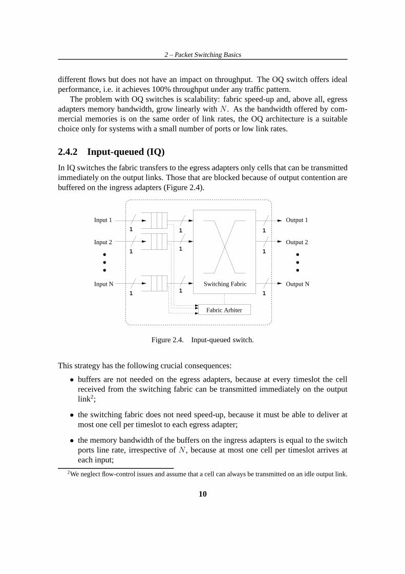
2.4.2 Input-queued (IQ)
In IQ switches the fabric transfers to the egress adapters only cells that can be transmittedimmediately on the output links. Those that are blocked because of output contention arebuffered on the ingress adapters (Figure 2.4).
1
1
1
1
1
Switching Fabric
1
Output 1
Output N
Output 2
1
1
1
Input 1
Input N
Input 2
Fabric Arbiter
Figure 2.4. Input-queued switch.
This strategy has the following crucial consequences:
• buffers are not needed on the egress adapters, because at every timeslot the cellreceived from the switching fabric can be transmitted immediately on the outputlink2;
• the switching fabric does not need speed-up, because it mustbe able to deliver atmost one cell per timeslot to each egress adapter;
• the memory bandwidth of the buffers on the ingress adapters is equal to the switchports line rate, irrespective ofN , because at most one cell per timeslot arrives ateach input;
2We neglect flow-control issues and assume that a cell can always be transmitted on an idle output link.
10

2 – Packet Switching Basics
• a scheduler is required to decide which among multiple cellscontending for thesame output will be transferred; the fabric must be configured accordingly.
In the simplest case, arriving cells are stored in FIFO queues and each ingress adaptercan only transmit the cell that is at the head of its queue. This constraint leads to aphenomenon called “Head-of-the-line (HOL) Blocking”: a cell that is at the head of itsinput queue and cannot be transferred because of output contention blocks all the othercells in the same queue. Blocked cells may be destined to outputs for which no other inputis contending, so the opportunity to transfer a cell is lost.HOL-blocking can severelydegrade performance: for large values ofN it limits switch throughput to about 58%under uniform i.i.d. traffic [8].
This level of performance is not acceptable, so in the past there have been many at-tempts to overcome the problem, in general by relaxing the FIFO constraint and allowingthe scheduler to consider multiple cells from the same queue. In recent years increasedCMOS densities have made feasible a new queueing architecture, called Virtual OutputQueueing, that completely eliminates HOL blocking and allows IQ switches to achievehigh performance.
2.4.3 IQ switches with Virtual Output Queueing (VOQ)
Virtual Output Queues (VOQs) are sets of independent FIFO queues, each of which isassociated to a specific output [9]. In an IQ switch it is possible to avoid HOL-blockingby deploying a set ofN VOQs on each ingress adapter (Figure 2.5). With VOQs, cells
1 1
11
Switching Fabric
1
1
Input N Output N
Output 1Input 1
Q1Q2
QN
Q1
QN
Q2
VOQ Set 1
VOQ Set N
...
...
Fabric Arbiter
Figure 2.5. Input-queued switch with Virtual Output Queues.
destined to different outputs can be served in any order and do not interfere with each
11

2 – Packet Switching Basics
Matching ProblemVOQ Status A Maximal Matching
Figure 2.6. A Bipartite Graph Matching (BGM) problem.
other; cells destined to the same output, on the contrary, are served with a FIFO policy topreserve the ordering of packets belonging to the same flow.
At every timeslot the scheduler must decide which cells to transfer through the switch-ing fabric, subject to the constraints that at most one cell can depart from an ingressadapter and at most one cell can be delivered to an egress adapter. The problem is equiv-alent to calculating a matching on a bipartite graph, as illustrated in Figure 2.6. Nodeson the left and right side represent fabric inputs and outputs respectively; dashed lines(edges) represent non-empty VOQs, i.e. cells that can be chosen for transfer. Amatchingis a set of edges such that each input is connected to at most one output and each outputto at most one input.
A matching ismaximum sizeif it contains the highest number of edges among allvalid matchings; it ismaximalif it is not possible to add new edges without removingpreviously inserted ones. For instance, the matching shownin Figure 2.6 is maximalbut not maximum: no edges can be added, but it is easy to verifythat there exists validmatchings with four edges. Edges can be assigned weights, such as the number of cellsenqueued in the corresponding VOQ, or the time the cell at thehead-of-the-line has beenwaiting for service. If weights are defined, theMaximum Weight Matching (MWM)is theone that maximizes the sum of the weights associated to the edges it contains.
IQ switches with VOQs can achieve 100% throughput under any i.i.d. traffic pattern,but only if very sophisticated scheduling algorithms are employed [10]. These algorithmsare in general difficult to implement in fast hardware and toocomplex to be executedin a single timeslot. However, as we will discuss in Section 2.5, a number of heuristicmatching algorithms that achieve satisfactory performance with reasonable complexity
12

2 – Packet Switching Basics
have been devised. Therefore input-queueing with VOQs is today the preferred architec-ture for the construction of large, high-performance packet switches. From this point on,when discussing IQ switches we will implicitly assume that VOQs are present.
2.4.4 Combined Input-Output-Queued (CIOQ) Switches
OQ and IQ switches represent two diametrically opposing points in the trade-off betweenspeed-up and scheduling complexity. The former employ maximum speed-up but re-quire no scheduling, the latter run without speed-up but need complex schedulers. CIOQswitches (with VOQs) represent an intermediate point: theybuffer packets both at theinputs and at the outputs, employ moderate speed-upS (1 ≤ S ≤ N) and use simplerschedulers.
Early simulation studies of CIOQ switches showed that, under a variety of switchsizes and traffic patterns, a small speed-up (between two andfive) leads to performancelevels close to those offered by OQ switches. These hints leda number of researchers toanalytically investigate the maximum performance achievable by CIOQ switches. Amongthe many results that were published, these are particularly significant:
• With a speed-upS = 2 and proper scheduling algorithms, a CIOQ switch canexactlyemulatean OQ switch, for any switch size and under any traffic pattern[11,12]. “Emulating” means producing exactly the same cell departure process at theoutputs given the same cell arrival process at the inputs.
• A CIOQ switch employing any maximal matching algorithm witha speed-up oftwo achieves 100% throughput under any traffic pattern, under the restriction thatno input or output is oversubscribed and that the arrival process satisfies the stronglaw of large numbers [13].
These results prove that with moderate speed-up the performance of an IQ switch canbe dramatically improved and that it can even reach the performance of an OQ switchif proper scheduling is used. A small fractional speed-up (S < 2) is also typically usedto compensate for various forms of overhead, such as additional headers that must beinternally prepended to cells and padding imposed by segmentation [14].
2.5 Scheduling Unicast Traffic in IQ Switches
2.5.1 Optimal Scheduling Algorithm
The optimal scheduling algorithms for an IQ switch, i.e. theone that maximizes through-put, is the Maximum Weight Matching (MWM), when queue lengths are used as weights [15].McKeown et al. noted that, with this choice of the weights, specific traffic patterns can
13

2 – Packet Switching Basics
lead to permanent starvation of some queues [10]. However, they also proved that 100%throughput is still achieved for any i.i.d. traffic pattern if the ages of HOL cells are usedas weights; in this case starvation cannot happen. The most efficient known algorithmfor calculating the MWM of a bipartite graph converges inO(N3 log N) time [16]. De-spite polynomial complexity, this algorithm is not practical for high-performance packetswitches, because it is difficult to implement in fast hardware and cannot be executed inthe short duration of a timeslot. For this reason, a number ofheuristic algorithms havebeen developed.
2.5.2 Parallel Iterative Matching Algorithms
Parallel iterative matching algorithms are the most popular class of heuristic matching al-gorithms. All inputs in parallel try to match themselves to one output by using a request-grant protocol. VOQ selection at the inputs and contention resolution at the outputs areperformed byarbiters (also calledselectors) using round-robin or random criteria. Theprocess is iterated multiple times, until a maximal matching is obtained or the maxi-mum number of iterations is reached. On average these algorithms converge inlog2 Niterations, but in the worst case they can takeN .
PIM
PIM [17] (Parallel Iterative Matching) is one of the first parallel iterative matching algo-rithms that have been proposed. In every timeslot the following threephasesare executedand possibly repeated multiple times:
1. Request:every unmatched input sends a request to every unmatched output forwhich it has a queued cell.
2. Grant: every output that has been requested by at least one inputrandomlyselectsone to grant.
3. Accept:if an input receives more than one grant, it selectsrandomlyone to accept.
The main disadvantage of PIM is that it does not perform well,as it achieves only63% throughput with a single iteration under uniform i.i.d.traffic. Moreover, it employsrandom selection, which is difficult and expensive to perform at high speed and can causeunfairness under specific traffic patterns [18].
RRM
RRM (Round-Robin Matching) [18] addresses some of the drawbacks of PIM by replac-ing random selection with round-robin. The selection logicat each input and output is
14

2 – Packet Switching Basics
composed by a round-robin selector and a pointer. Pointers at the outputs are namedgrant pointers, whereas those at the inputsaccept pointers.
Every iteration of RRM entails the following three phases:
1. Request:every unmatched input sends a request to every output for which it has aqueued cell.
2. Grant: every output that has been requested by at least one input selects one togrant in round-robin order, starting from the position indicated by the grant pointer.The pointer is advanced (moduloN) to one input beyond the one just granted.
3. Accept: if an input receives more than one grant it selects one to accept in round-robin order, starting from the position indicated by the accept pointer. The pointeris advanced (moduloN) to one output beyond the one just accepted.
The performance of RRM is very close to that of PIM, so still quite poor.
i-SLIP
i-SLIP [19] is a improvement of RRM that, with an apparently minor modification,achieves much higher performance. The three phases are modified as follows:
1. Request:same as RRM.
2. Grant: every output that has been requested by at least one input selects one togrant in round-robin order, starting from the position indicated by the pointer. Thepointer is advanced (moduloN) to one input beyond the one just grantedif and onlyif the released grant is accepted in the accept phase.
3. Accept:same as RRM.
Moreover, the grant and accept pointers are updated only in the first iteration; a detail thatis crucial to prevent starvation of any VOQ under any traffic pattern.
i-SLIP performs extremely well: under uniform i.i.d. trafficit achieves 100% through-put with a single iteration, because it guaranteesdesynchronizationof the grant pointers.When the switch is loaded at 100% and traffic is uniform i.i.d,all VOQs are backlogged.Assume that the grant pointers at multiple outputs point to the same input, i.e. theyaresynchronized. The input receives multiple grants, accepts one and moves the acceptpointer. Thanks to the modification of the grant phase, only one of the grant pointers (theone corresponding to the grant that has been accepted) is moved and leaves the group. Forthe same reason, at most one new grant pointer can join the group. It is possible to provethat, after a transient period, all grant pointers point to different inputs, regardless of theirinitial position. Amaximummatching is produced at every timeslot and 100% throughput
15

2 – Packet Switching Basics
is achieved. Desynchronization is preserved as long as all VOQs are non-empty, becauseall the released grants are accepted and so all the grant pointers move “in lockstep”.
Another important feature ofi-SLIP is that it is fair and starvation free, i.e. it doesnot favor some flows over others and guarantees that a cell at the head of a VOQ will beserved within finite time.
DRRM
DRRM [20] (Dual Round-Robin Matching) is a further variant of i-SLIP that achievessimilar performance with one less phase and less information exchange between the inputand the outputs.
The two phases performed in each iteration are:
1. Request:every unmatched input selectsoneunmatched output to request in round-robin order, starting from the position indicated by arequest pointer. In the firstiteration, the pointer is updated to one position beyond theinput just requested(moduloN) if and only if a grant is received in thegrant phase.
2. Grant: each output that has been requested by at least one input selects one to grantin round-robin order, starting from the position indicatedby a grant pointer. Inthe first iteration the pointer is updated to one position past the input just granted(moduloN).
A grant phase is not required because each input requests only one output, so it can receiveat most one grant, which is automatically accepted.
DRRM achieves 100% throughput under uniform i.i.d. traffic because in this situationrequest pointers (moved only if a grant is received) desynchronize.
Figure 2.7 shows the operation of the DRRM algorithm for a4× 4 switch. At the endof the first iteration all pointers (except R4 and G1) are moved forward by one position.As the matching is maximal, it is not necessary to perform additional iterations.
FIRM
FIRM [21] is an improvement ofi-SLIP that achieves lower average latency by favoringFCFS order of arriving cells. It does so by introducing a minor modification in the pointerupdate rule of the grant phase ofi-SLIP: in the first iteration, if a grant is not accepted, thegrant pointer is moved to the granted input. The authors also show that this modificationreduces the maximum waiting time for any request from(N − 1)2 + N2 to N2.
A similar modification has been proposed for DRRM in [22].
16

2 – Packet Switching Basics
1
34
2
1
34
2
1
34
2
1
34
2
1
34
2
1
34
2
1
34
2
1
34
2
RequestsRequest
VOQ Status Grants PointersGrant
Request Phase Grant Phase
Pointers
R1
R2
R4
G1
G2
G3
G4
R3
Figure 2.7. The behavior of the DRRM algorithm in a sample scenario.
Weighted Algorithms
As an attempt to approximate the behavior of MWM and improve performance undernon-uniform traffic, heuristic iterative weighted algorithms have been developed. Amongthese arei-OCF (Oldest Cell First),i-LQF (Longest Queue First) andi-LPF (Longest PortFirst), proposed by Mekkittikul and McKeown [23].
2.5.3 Sequential Matching Algorithms
Sequential scheduling algorithms produce a maximal matching by letting each input addan edge at a time to an initially empty matching.
RPA [24] (Reservation with Pre-emption and Acknowledgement) and RRGS [25](Round Robin Greedy Scheduler) are examples of sequential matching algorithms. Aninput receives a partial matching, adds an edge by selectinga free output and passes iton to the next input. Inputs considered first are favored, because they find most outputsstill available. To avoid unfairness, the order in which inputs are considered is rotated atevery timeslot. These algorithms always produce a maximal matching, are fair and can bepipelined to improve the matching rate. However, they require strong interaction amongthe inputs and introduce latency at low load when pipelined.
The Wavefront Arbiter [26] (WFA) is another popular sequential arbiter. The statusof all theN2 VOQs of the system is represented in aN × N request matrixR: Ri,j = 1
17

2 – Packet Switching Basics
if input i has a cell destined to outputj, 0 otherwise. Sets of VOQs that are positionedon a diagonal of the matrix are conflict-free, because they correspond to cells enqueuedat different inputs and destined to different outputs. Hence it is possible to produce amatching by sequentially “sweeping” all the diagonals of the request matrix, excludinginput and outputs that have already been matched. WFA is fast, simple and offers goodperformance; however, it suffers from some minor fairness and implementation issues [7].
2.6 Scheduling Multicast Traffic in IQ Switches
Traffic generated by a single source and directed to multipledestinations is calledmulti-cast. One-to-many communication is important for many applications (see Section 6.1)so switches must be able to efficiently replicate packets to multiple output ports.
In an IQ switch replication can be achieved simply by transmitting cells through theswitching fabric multiple times, one for every egress adapter that must be reached. How-ever, the crossbar has intrinsic multicasting capabilities and can replicate a cell to multipleoutputs in a single timeslot. A scheduler that takes advantage of this feature can reducethe latency experienced by cells and the load on the fabric input ports, which are occupiedfor only one timeslot.
In this section we briefly introduce the problem of scheduling multicast traffic andpresent some of the most popular scheduling algorithms.
2.6.1 Definitions
The set of outputs a multicast cell is destined to is called the fanout setand its cardinalitythe fanout3. For clarity, we distinguish between theinput cell that is transmitted to theswitching fabric and theoutput cellsthat are generated by the replication process.
A scheduling discipline is termedfanout splittingif it allows partial service of aninput cell, i.e. if the associated set of output cells can be transferred to the outputs overmultiple timeslots.No fanout splittingdisciplines, on the contrary, require all the outputcells associated to an input cell to be delivered at the outputs in the same timeslot. Fanoutsplitting offers a clear advantage because it allows the fabric to deliver in every timeslotas many cells as possible to the outputs, at the price of a small increase of implementationcomplexity.
The residueis the set of all output cells that lose contention for outputports in atimeslot and have to be transmitted in subsequent timeslots.
3The term “fanout” is often used to refer also to the set itself.
18

2 – Packet Switching Basics
2.6.2 Queueing
A multicast cell can be destined to any subset of theN outputs, so the number of possiblefanout sets is2N−1. Even for moderate values ofN it is not practically feasible to providea dedicated queue to cells with the same fanout set, therefore HOL-blocking cannot becompletely eliminated. Indeed, most architectures store cell arriving on an ingress adapterin a single queue and serve them in FIFO order.
To alleviate HOL-blocking, in [27] the authors propose a windowing scheme thatallows the scheduler to access any cell in the firstL positions of the queue. This schemeoffers throughput improvements, but requires random-access queues, which are complexto implement. Moreover, it is clearly not effective under bursty traffic.
In [28] and [29] the benefits that can be gained by using a smallnumber of FIFOqueues at each ingress adapter are investigated. When multiple queues are present, itis necessary to define a queueing policy. Static queueing policies always enqueue cellswith a given fanout in the same queue, whereas dynamic policies may enqueue them indifferent ones, depending on status parameters such as queue occupancy. Static policieslose effectiveness when few flows are active, because most ofthe available queues mayremain empty, whereas dynamic policies lead to out-of-order delivery.
In [30] maximum switch performance is analyzed, under the hypothesis that a queueis provided for every possible fanout set. The results of this work have great theoreticalinterest, because they show that an IQ switch is not able to achieve 100% throughputunder arbitrary traffic patterns, even if it employs this ideal queueing architecture and theoptimal scheduling discipline.
2.6.3 Scheduling
The problem of scheduling multicast traffic in an input-queued switch has been addressedby a number of theoretical studies. In [31] and [32] the performance of various schedulingdisciplines (such as random or oldest-cell-first) is analyzed under different assumptions.Work in [33] studies the optimal scheduling policy, obtaining it for switches of limitedsize (up to three inputs) and deriving some of its propertiesin the general case.
In [34] the authors take a more practical approach: they specifically target the designof efficient and implementable scheduling algorithms when FIFO queueing is used andfanout splitting allowed. They provide important insight on the problem and proposevarious solutions with different degrees of performance and complexity. An importantobservation is that at any timeslot, given a set of requests,all non-idlingpolicies (thosethat serve as many outputs as possible) transmits cells to the same outputs and leave thesame residue. What differentiates one policy from the otheris residue distribution, i.e. thecriteria with which the set of output cells that have lost contention is partitioned among theinputs. Aconcentratingpolicy assigns the residue to as few inputs as possible. Policiesexhibiting this property serve in each timeslot as many HOL cells as possible, helping new
19

2 – Packet Switching Basics
cells to advance to the head of the queue. As new cells may be destined to idle outputs,throughput is increased. Actually a proof is given that for a2×N switch a concentratingpolicy is optimal, but it cannot be extended to switches of arbitrary size.
The first proposed algorithm, called “Concentrate” implements a purely concentratingpolicy. However, the authors note that the algorithm suffers from fairness issues, as it canpermanently starve queues, so they proceed with the design of TATRA, a concentratingalgorithm with fairness guarantees. As TATRA is difficult toimplement in hardware, theyfurther propose the Weight Based Algorithm (WBA). WBA is a heuristic algorithm thatapproximates concentrating behavior by favoring cells with small fanout and guaranteesfairness by giving priority to older cells. The algorithm works as follows:
1. At the beginning of every cell time each input calculates the weightof the cell atthe head of its queue, based on the age of the cell (the older, the heavier) and thefanout (the larger, the lighter).
2. Each input submits a weighted request to all the outputs that it wishes to access.
3. Each output independently grants the input with the highest weight; ties are brokenrandomly.
In the specific implementation shown in the paper, the weightis calculated adW =αA − φF , whereA is the age (expressed in number of timeslots),F is the fanout andα andφ are multiplication factors that allow tuning of the scheduler for performance orfairness. Largeα implies that older cells are strongly favored, improving fairness, whilelargeφ penalizes cells with large fanout, exalting the concentrating property and thusimproving performance. Calculations show that a cell has towait at the head of the queuefor no longer than(N(φ/α + 1) − 1) timeslots. WBA can be easily implemented inhardware, as reported in the paper.
20

Part I
A Switching Architecture forShared-Memory Supercomputers

Chapter 3
Supercomputers and InterconnectionNetworks
In this chapter we present a brief overview of High-Performance Computing (HPC) sys-tems, also calledsupercomputers. We first describe the main architectural traits of asupercomputer, including the organization of the computing nodes, the partitioning ofthe memory space and the programming model. We then focus on the interconnectionnetwork(sometimes simply called “the interconnect”), discuss itsrole in the system andanalyze the main requirements. Finally, we introduce two fundamental classes of in-terconnection networks, highlight their most important features and show some sampletopologies.
3.1 Supercomputing Systems
A supercomputeris “a computing system (hardware, system software and applicationssoftware) that provides close to the best currently achievable sustained performance ondemanding computational problems” [35]. In the past the growth in demand for com-puting power has mainly been driven by scientific (weather forecasting, computationalbiology, plasma physics, etc.) and defense applications (cryptanalysis, stockpile steward-ship, etc.). Nowadays business applications (automotive and aircraft design, geologicalanalysis, modeling of financial markets, etc.) are also playing a role.
For almost two decades microprocessors have experienced a tremendous growth inperformance, mainly due to technological improvements. Now the growth rate is slow-ing down, because of complicated issues such as power dissipation and difficulties inmanaging design complexity. Computer designers have traditionally tried to push the per-formance of computing systems by building parallel machines, in which multiple com-puting nodes work concurrently on portions of the same problem. In the near future we
22

3 – Supercomputers and Interconnection Networks
can expect parallelism to become the major source of performance improvement for allcomputing systems.
A large number of parallel computer architectures have beenproposed over the years,varying considerably in terms of applications, programming model and intended systemsize. While it is difficult to provide a single, comprehensive taxonomy for this large anddiverse set of architectures, some useful dichotomies for positioning and comparison ofdifferent systems have been established.
3.1.1 Shared-Memory vs. Message-Passing
In a shared-memory system all available memory can be accessed by all processors bymeans of a global address space. Processors exchange data and synchronize by access-ing shared memory locations. Load/Store instructions issued by a processor are implic-itly converted to Read/Write messages that the interconnection network delivers to theappropriate memory bank.
In a message-passing system, on the contrary, each processor has its own private mem-ory space. Programmers explicitly exchange data and synchronization information amongprocessors by invoking message passing primitives.
In general shared-memory systems are easier to program (at the operating system,compiler and application level) but more difficult to designthan message-passing sys-tems. On the other hand, the hardware simplicity of message-passing systems, especiallythe lack of complex cache-coherency issues, makes them muchmore scalable. For thisreason, the majority ofMassively Parallel Processing(MPP) systems, having thousandsor even hundreds of thousands of processors, are message-passing machines.
3.1.2 UMA vs. NUMA
In a shared-memory machine memory can be logically placed ina single centralized lo-cation or distributed over the computing nodes, co-locatedwith the processors. In the firstcase memory access time isuniform, i.e. it does not depend on which processor accesseswhich memory location. In the other, it isnon-uniform, because a processor experienceslower access time when accessing a memory location in its local bank rather than in aremote one. Machines providing uniform or non-uniform memory access are classified asUMA and NUMA, respectively.
Typical UMA systems are SMP (Symmetric Multiprocessor) machines, in which asmall number of processors (few tens at most) and a single bank of memory are connectedby means of a simple interconnection (usually a shared bus),as shown in Figure 3.1.Examples of NUMA systems are DSM (Distributed Shared-Memory) machines, whichcomprise hundreds of computing nodes (composed by a processor and a memory bank)interconnected through a high-speed network (Figure 3.2).
23

3 – Supercomputers and Interconnection Networks
Memory Memory Memory
Processor
Cache
Processor
Cache
Processor
Cache
Interconnection Network
Figure 3.1. An SMP machine
Memory Memory Memory
Processor
Cache
Processor
Cache
Processor
Cache
Interconnection Network
Figure 3.2. A DSM machine
24

3 – Supercomputers and Interconnection Networks
3.1.3 Custom vs. Off-the-shelf
Various platforms use different blends of custom and commercial, off-the shelf (COTS)components. COTS components are designed for a broad range of applications and areproduced in large quantities. They benefit from economies ofscale and offer very goodcost/performance ratios. On the other hand, their design isnot optimized for supercom-puting and they might perform poorly on some specific applications.
Microprocessors
The cost of designing and manufacturing a new processor has grown steadily over theyears and nowadays only few companies can afford it. For thisreason, most super-computers today use commodity processors produced for the large-volume server andworkstation markets.
Interconnects
The interconnection network, on the contrary, is more difficult to build with commoditycomponents. The gap between the requirements of a local areanetwork and those of asupercomputer interconnect is quite large. Although the bandwidth offered by Ethernethas increased by several orders of magnitude during its lifetime, its application domain isstill limited by its inability to achieve low latency and guarantee lossless behavior.
New standard-based technologies, Infiniband [36] in particular, are trying to fill thegap and provide a unified network infrastructure for local area networking and parallelcomputing. Infiniband has a number of features specifically aimed at reducing networklatency. It employs an improved node/network interface that allows the network adapter toconnect directly to the memory controller of the node, bypassing the I/O bus. Moreover,it supports advanced communication paradigms, such as RDMA, that allow a node tomove data directly in and out the memory space of another node. A carefully designedflow-control mechanism enables loss-free operation and allows prioritization of latency-sensitive messages. Altogether this characteristics makeInfiniband a potential alternativeto custom interconnection networks.
Clusters
Many of the largest supercomputers available today arecluster, i.e. collections of stan-dard servers and workstations, loosely connected through standard LAN interconnectssuch as Gigabit Ethernet. As clusters are entirely composedby commodity components,they offer excellent cost/performance ratios. The use of standard interconnects promotesscalability, while the fact that each node has its own processor, memory and operatingsystem provides significant advantages in terms of reliability and fault-tolerance [37].
25

3 – Supercomputers and Interconnection Networks
Figure 3.3. Time evolution of the architecture of the 500 most powerful supercomputersin the world (fromhttp://www.top500.org).
Clusters performance is mainly limited by the latency introduced by the network,which makes them unfit for applications that require strong interaction among computingnodes. On the other hand, popular applications such as web servers and databases areparticularly amenable to run on clusters, because they are characterized by a large numberof independent threads that work in parallel, so they are notpenalized by network latency.For example, in [38], the authors describe the Google cluster, built with standard PCs andcomprising more than 6000 processors (as of December 2000).
Figure 3.3 shows the distribution of the 500 most powerful supercomputers in theworld, based on their architecture. The current list is clearly dominated by clusters andconstellations (clusters of SMP systems) that together account for 80% of the total. Theremaining 20% is represented by custom MPP systems.
3.2 Interconnection Networks
The interconnection network is a critical component of a supercomputer, because it has adirect impact on performance and scalability. The variety of node architectures, program-ming models and application requirements has generated a proliferation of interconnec-tion network designs, ranging from single shared busses used in SMP systems to complex,meshed fabrics with thousands of ports for MPP systems.
The key requirements of a supercomputer interconnect are:
• Low latency Latency is the time required for a packet to traverse the network.
26

3 – Supercomputers and Interconnection Networks
It is the most important performance metric of an HPC interconnect, especiallywhen considering shared-memory machines. In such systems communication istriggered by memory access instructions and the latency introduced by the networkdirectly contributes to memory access time. Specialized processors use latency-hiding techniques, such as fetching data from memory in advance [39], fetch-ing more than necessary and allowing multiple outstanding memory references.Despite the availability of these techniques, network latency remains the primaryperformance bottleneck for a number of applications [35].
• High Throughput Throughput is a measure of therate at which the network candeliver data to the nodes. High throughput corresponds to high utilization of linkbandwidth and is particularly important when the nodes haveto exchange bulk setsof data. Latency-hiding techniques mentioned above tend totransfer large blocksof data, thus increasing throughput requirements.
• Scalability The network must be able to interconnect a large number of comput-ing nodes. Moreover, as the number of nodes grows, the aggregate bandwidth ofthe network should increase proportionally and latency should remain low. Net-work scalability is essential to guarantee that the computing capacity of the systemreaches the intended levels and improves as new nodes are added.
• Reliability and Fault Tolerance A supercomputer uses a large number of com-ponents and, as a consequence, the failure rate can be high. The network shouldbe able to continue operation in presence of a limited numberof faults. In partic-ular, it should be able to exploit meshed connectivity and re-route messages overalternative paths in case of link or node failure.
Interconnection networks can be characterized in terms oftopology, routingandflow-control. Topology describes the interconnection pattern among nodes, routing determinespaths between pairs of non-adjacent nodes and flow-control defines mechanisms to reg-ulate message transmission among nodes and prevent networkoverloading. Selectingthe topology is usually the first step in designing the network, because routing and flow-control are heavily dependent on its characteristics. The choice of the topology is mainlydriven by the constraints imposed by the available packaging technology [7].
In the remaining part of this section we briefly describe two important classes of inter-connection networks and show some popular topologies. A comprehensive classificationcan be found in [40].
3.2.1 Direct networks
The distinguishing property of direct networks is that eachnode is directly connected to asmall set of other nodes by means of bi-directional, point-to-point links. Communication
27

3 – Supercomputers and Interconnection Networks
between non-neighboring devices entails transmission through intermediate hops. Eachnode has an integratedrouter that handles communications, transmitting and receivingmessages or relaying them to other nodes.
Popular topologies for direct networks aren-dimensional meshes, tori and hypercubes(Figure 3.4). The tree (Figure 3.5) is another important topology, because it efficientlysupports one-to-many and many-to-one communication patterns, typical of synchroniza-tion andcollectiveoperations that require coordination of many computing nodes [40].
Direct networks scale very well in terms of bandwidth, so they have been used exten-sively in MPP systems. However, as the number of nodes increase, so does the distancebetween pairs, thus latency degrades.
Very large systems can use multiple networks optimized for specific tasks. For ex-ample, the IBM Blue Gene/L, capable of scaling up to 65535 computing nodes, usesa 3D-torus as a general-purpose interconnect and two specialized tree-like networks forsynchronization and collectives [41,42].
3.2.2 Indirect networks and MINs
Indirect networks interconnect computing nodes through intermediate nodes calledswitches(Chapter 2). Switches receive messages on input ports and forward them to the appropri-ate output ports, towards the final destination.
The complexity of a switch typically grows quadratically with the number of ports,so its scalability is limited to few hundred ports at most (Section 2.3). As a single switchcannot satisfy the requirements of large supercomputers, we must turn toMultistage In-terconnection Networks (MINs). MINs enable the construction of fabrics interconnectingthousands of nodes by employing several switches arranged in multiplestages. The num-ber of stages and the interconnection pattern between the switches define the topology ofthe network.
MINs were originally studied for circuit-switched networks and later employed inpacket-switched networks. Among the most popular topologies are Clos [43,44], Butter-flies [45] and Fat-trees [46] networks.
A MIN is unidirectionalif data can flow on network links in a single directional,bi-directional if it can flow simultaneously in both directions. For computer interconnects,bi-directional MINs are usually preferred, because they offer shorter paths between nodes(messages traverse only as many stages as necessary) and better redundancy. Figures 3.6and 3.7 show a bi-directional Butterfly and a Fat-Tree network (circles represent nodesand boxes represent switches).
MINs have very good scalability properties because the aggregate bandwidth growsas new switches are added to the network and latency remains low thanks to small numberof stages. However, cost also increases rapidly, because more and more switch ports areused to connect to other switches rather than computing nodes.
28

3 – Supercomputers and Interconnection Networks
(a) (b)
(c)
Figure 3.4. Direct network topologies: (a) 2D-mesh, (b) 2D-Torus, (c) Hypercube
Figure 3.5. A 15-nodes binary tree topology
29

3 – Supercomputers and Interconnection Networks
Figure 3.6. An 8-nodes bi-directional butterfly network
Figure 3.7. An 8-nodes fat-tree network
30

Chapter 4
The OSMOSIS Project
In this chapter we present the OSMOSIS project, aimed at developing a prototype of aswitch for shared-memory supercomputers. We start with a digression on the role of elec-tronics and optics in packet switching, to explain the rationale behind the choice of anelectro-optical architecture and compare it briefly with other optical switching architec-tures. We then provide an overview of the system, discussingthe set of requirements andthe design of the the data- and control-path.
4.1 Electronics and optics in packet switching
4.1.1 Electronic switching
The performance of electronic packet switches has grown tremendously in the last fifteenyears, driven by the exponentially-increasing bandwidth requirements of Internet traffic.Electronic switching is now a mature technology that has been employed in a numberof other domains, including HPC systems. However, the toughlatency and scalabilityrequirements of HPC interconnects are pushing it to the limit and are exposing its weakestpoints.
The major problem that plagues electronic switching today is power consumption. Asthe line rates increase, it becomes more and more difficult todrive copper cables overacceptable distances. It is currently estimated that as much as 50% of the power con-sumed by a switch is actually spent on the cables [14]. The problem can be addressed byusing optical fibers for transmission on the links and electronic components for buffering,switching and processing. This solution, however, is only partially satisfactory, becausethe O/E/O conversions required at the ingress and egress side of the switch consumepower, increase the cost of the devices and introduce latency. It would be highly desirableto switch packets in the optical domain, avoiding conversion and reduce latency to thetime-of-flight of signals in the fibers.
31

4 – The OSMOSIS Project
4.1.2 Optical devices
Optical devices have a number of unique features that distinguish them from electronicones and make them extremely attractive. First, a single fiber link, thanks to DWDMtechniques, can offer bandwidths on the order of terabits per second, several orders ofmagnitude larger than what is provided by electrical links.Second, optical links canspan very long distances using limited power, so they are particularly fit for large anddistributed computing systems, whose diameters can be in the order of tens or hundredsof meters. Last, and probably foremost, many optical devices are data-rate transparent,meaning that they have extremely large operational bandwidths and can operate on signals(split, combine, amplify, etc.) at constant power, regardless of the frequency at whichthey are modulated. In the electronic domain, on the contrary, devices can only operatein specific frequency ranges and power consumption is proportional to frequency. Thanksto these features, an all-optical data-path can scale in bandwidth by orders of magnitude,without increasing the physical size or the power consumption of the network elements.
The development of optical switches has mainly been limitedby factors such as de-vice cost, integrability and noise levels. Moreover, the lack of optical buffers and logicelements are two fundamental issues that haven’t been addressed satisfactorily yet. How-ever, it is a common opinion that economic and technologicalissues can be solved inshort timeframes. If optical devices get market acceptance, their cost will decrease andthe manufacturing process will improve, leading to higher quality and integration levels.As Moore’s Law, that governs density as well as cost of electronic components, is slowingdown, projections show that optical switches could be economically competitive by theend of the decade [47].
4.1.3 Optical switching architectures
Over the years many optical switching architectures have been proposed [48]. Many ofthem, however, are conceived for circuit-switching networks, so they exploit physicalphenomena that enable switching times in the order of milliseconds.
For packet-switching networks, the switching time must be smaller than the durationof a minimum-size packet. Given the line-rates and packet sizes we are targeting, thistranslates to few nanoseconds. Optical Burst Switching (OBS) techniques mitigate thischallenging requirements by fitting multiple packets in large containers and switchingthem together at once. These techniques are not suitable forsupercomputing applica-tions because packets must wait for a container to be full before being switched, so theyexperience additional latency.
Semiconductor Optical Amplifiers (SOAs) are the most promising technology for op-tical packet switching. They can be viewed as ON/OFF opticalswitching elements, withvery low switching times (on the order of few nanoseconds), high extinction ratios andlow noise. They are compact, consume low power and can be integrated into arrays [49].
32

4 – The OSMOSIS Project
SOAs can be used to build switching nodes ranging from simple2 × 2 switches to largecrossbars using broadcast-and-select networks [50].
Even with appropriate technology, the question remains on how to build a packetswitch without large buffers and bit-level processing capabilities. A possible approach isto use electronics for buffering and control at the borders of the fabric, confining optics tothe data-path. The basic philosophy behind such hybrid opto-electronic architectures is touse optics for what optics does best and electronics for whatelectronics does best [51].
An alternative, pursued by the Data Vortex project [52], is to eliminate the need forbuffers altogether by using deflection routing and a very simple node structure that en-ables distributed control with minimal processing capabilities. The Data Vortex aims atfully exploiting the benefits of optical technologies and being a true all-optical switch. Ithas a number of desirable features that make it very attractive for supercomputing applica-tions, first and foremost scalability. However, it also has some non-negligible drawbacks,mainly low throughput per port, out-of-order delivery and hard-to-predict latency.
4.2 The OSMOSIS System
4.2.1 Goals and requirements
OSMOSIS (Optical Shared-MemOry Supercomputer Interconnect System) is a researchproject jointly developed by IBM and Corning that aims at building an HPC switch withan all-optical data path and an optimized electronic control path [53].
The goals of the project are twofold: on one side, it aims at solving the technicalchallenges involved in building a demonstrator system thatmeets a set of ambitious re-quirements, on the other it aims at accelerating the cost reduction of all-optical switches,achieving denser integration levels of optical componentsand finding a high volumemarket for them, in addition to the low volume HPC market.
The specific requirements for the demonstrator are:
Port count 64 (single stage) – 2048 (multistage)Line rate 40 Gb/s (scalable to 160 Gb/s)Total (application to application) latency< 1µsEffective user bandwidth > 75% of raw transmission bandwidthBit Error Rate (BER) < 10−21
Packet delivery Reliable and in-order
In addition, efficient support for mutlicast and broadcast is a basic requirement, as theyare particularly important for HPC applications [54]. All electronic control logic must beimplemented using only FPGAs and commercial components, togain flexibility and keepthe cost of the demonstrator acceptable.
33

4 – The OSMOSIS Project
(Scheduler)
Optical Switch Controller Module
WDMMux Coupler
Star
AmplifierOptical
8x1 1x128
λ 1
λ 2λ 3λ 4λ 5λ 6λ 7
λ 8
control
RXEQ
control
RXEQ
control
TX
64
1VOQs
control
TX
64
1VOQs
uCCτ
dCCτ
uDCτdDCτ
SCCτ
8x1 8x11x8
Combiner
Ingress HCAs (64x) Egress HCAs (64x)Optical Selection Modules (128x)Optical Broadcast Modules (8x)
EDFA
Fast SOA 1x8Fiber SelectorGates
Fast SOA 1x8WavelengthSelector Gates
Figure 4.1. OSMOSIS system architecture.
4.2.2 System Overview
From an architectural point of view, OSMOSIS is a synchronous CIOQ switch (Chap-ter 2). This implies that the switch operates on fixed-size cells and the optical core,functionally equivalent to a crossbar, is reconfigured on a cell-by-cell basis. The cellsize derived from the requirements set is 256 B [55]. In general shorter cells would bedesirable, as they would offer lower latency and improve efficiency. However, this cellsize is acceptable and well-suited for shared-memory supercomputing, as synchronizationmessages and cache-coherency transactions usually comprise a 100-300 B payload.
Figure 4.1 shows the high-level architecture of OSMOSIS in single-stage configura-tion. The system is composed by a set ofadaptersinterconnected by anoptical corecontrolled by a centralizedscheduler.
Adapters have two separated but physically co-located parts, namedingressandegressadapter, that handle cells entering and exiting the switch respectively. They perform in-terfacing functions between the computing nodes and the interconnect, including E/O andO/E conversions, cells buffering and processing. Every ingress adapter comprises a fullset ofN VOQs, in which it stores cells based on their destination anda corresponding setof N reliable delivery queues (RDQs). Egress adapter host anegress queuewhere theybuffer received cells before delivering them to the computing node or transmitting themto the next stage. Every adapter has a dedicated optical control link to the centralizedscheduler, which carries the control channel protocols.
The scheduler is located on a separate card close to the optical switching core. Atthe beginning of every timeslot it receives requests to transmit from the ingress adapters,resolves conflicts and grants selected adapters, authorizing them to transmit.
34

4 – The OSMOSIS Project
4.2.3 Data path
Every adapter is assigned a specific wavelengthλi, chosen among eight possible wave-lengths. The 64 adapters are logically divided in eight groups, in such a way that all theadapters in the same group use a different wavelength.
The switching function is implemented with aBroadcast & Selectarchitecture thatcombines eight-way space- and eight-way wavelength-division multiplexing to imple-ment a 64-port fabric. The first stage of the optical core consists of eightbroadcast unitsthat receive the signals transmitted by a group of adapters (consisting of eight signals oneight different wavelengths), multiplex them on a single fiber, amplify the resulting WDMsignal using an erbium-doped fiber amplifier (EDFA) and then split it to 128 waveguides1.The selectstage comprises 128 planes, two per output port, each connected to all theeight broadcast units of the first stage. A group of eight SOAsperforms fiber selectionby blocking signals coming from all the broadcast units except one. Regardless of the se-lected fiber, the WDM signal is passed through a combiner to guide it to a common fiberand then de-multiplexed to separate the eight wavelengths on different fibers. A secondgroup of SOAs is used to select a single wavelength and block the others. The signal isagain guided to a common fiber by means of a combiner and finallyreaches the egressadapter. Each egress adapter is connected to two select units, so it can independently re-ceive two signals at the same time. Multicast and broadcast transmission can be achievedsimply by having multiple planes select the same fiber/colorpair.
The optical core employs a combination of Planar Lightwave Circuits (PLCs) anddiscrete components. Transmission from the ingress adapters must be synchronized insuch a way that cells arrive at the optical crossbar at the same time, when SOAs have justbeen configured, and walk equal-length paths. This is achieved by using a global clocksignal distributed to all the adapters and components whoselength is matched to a fractionof the optical packet length.
Although all ports work at the same nominal bit-rate, egressadapters receive bit-streams generated by different serializers, with independent phases. Thus receivers mustoperate in burst-mode and, to keep cell overhead low, they must be able to recover bit-phase in a very short time. Moreover, channels use differentwavelengths, so receiversmust have wide-dynamic-range transimpedance.
4.2.4 Control path
The physical implementation and packaging constraints of OSMOSIS, and of large switchesin general [14], lead to a distribution of switch components(adapters, optical core, sched-uler) over multiple racks, interconnected by long cables. The latency introduced by thesecables, together with the delay due to (de-)serialization and other contributions, add up
1128-way splitting (rather than 64-way) is required to alloweach egress adapter to receive up to twocells per timeslot. The details about the usage of the secondreceiver can be found in [54]
35

4 – The OSMOSIS Project
to several cell times and must be carefully taken into account in the design of the controlpath.
Further details about the architecture of the OSMOSIS scheduler and the design of thecontrol plane can be found in [54].
Control Channel Protocol
As the scheduler is connected to the adapters through long cables, control messages haveto be pipelined. The scheduler has delayed knowledge of the status of the VOQs at theingress adapters, an issue that can seriously degrade performance. The problem is ad-dressed by maintaining VOQ status information at the scheduler, updating it using anincrementalprotocol [56] and ensuring its consistency using acensusmechanism [57].
The scheduler maintainsN2 counters, each representing the occupancy of a VOQ.When a new cell arrives at an adapter, the scheduler is notified by a control message andincrements the corresponding counter. When the scheduler issues a grant, it decrementsthe counter, as the cell will be dequeued as soon as the grant arrives at the adapter.
The census mechanism is a distributed consistency protocolcapable of detecting andcorrecting discrepancies between the information maintained at the scheduler and theknown status of the VOQs on the adapters. It is triggered at regular intervals to ensureproper recovery from control channel transmission errors.
Scheduler
The scheduler must solve a bipartite-graph matching problem at every timeslot (Sec-tion 2.4.3). As the optimal scheduling algorithms is not implementable in fast hardware,the scheduler uses a heuristic iterative algorithm based onDRRM (Section 2.5.2 and [20]).Iterative algorithms are implemented using2N programmable priority encoders, that per-form 1-out-of-N selection [28]; asN increases, so does their space and time complexity.Moreover, they need to performlog
2N iterations to produce a good matching and achieve
high delay-throughput performance.Given thatN is large and that only FPGAs are at disposal, implementing the schedul-
ing algorithm and performing the desired number of iterations entails a number of chal-lenges. First, the scheduler must be distributed over multiple chips, as it doesn’t fit on asingle one. Distribution requires the usage of specific techniques to deal with delays andbandwidth limitations of in chip-to-chip communication. These techniques are part ofthe contributions of this work and are discussed in detail inChapter 5 and [58]. Second,it is not possible to perform the desired number of iterations in the short duration of atimeslot. To overcome the problem, the scheduler employs a pipelining scheme, calledFLPPR (Fast Low-latency Parallel Pipelined aRbitration) [59]. The most important fea-ture of FLPPR, that distinguishes it from previously proposed pipelining schemes [60,61]
36

4 – The OSMOSIS Project
is that new requests are allowed to enter at any stage of the pipeline, reducing the mini-mum latency to a single timeslot. FLPPR also achieves betterperformance at high loadunder non-uniform and bursty traffic.
The scheduler also implements a novel scheme to achieve fairand efficient integratedscheduling of unicast and multicast traffic. The scheme is described in Chapter 6 and [62].
Reliable Delivery
The optical data path is engineered to achieve a raw bit-error rate of10−10. A customforward error-correcting code (FEC) is employed to reduce it to 10−17. Cells that cannotbe corrected by the FEC must be retransmitted, hence each adapter has a set of reliable-delivery queues (RDQs) where packets are stored until the egress adapter acknowledgesreception. ACKs are transmitted on the control channel and aGo-Back-N retransmissionpolicy is used. This policy is simple to implement and is consistent with the bursty na-ture of optical link errors. As the error rate provided by theFEC is already fairly low,retransmission is rarely required and the inefficiencies ofGo-Back-N are not an issue.
Flow Control
To prevent overflow of the egress buffers, the system employ an on-off flow control loopbetween egress adapters and the scheduler, which is embedded in the upstream controlchannel messages. If a specific egress buffer is close to saturation, the scheduler no longerconsiders any request for the corresponding output. When occupancy decreases below apre-determined threshold, the permission is reinstated.
4.2.5 Multistage scalability
One of the main objectives of the OSMOSIS project is to provide a system that can scaleto thousands of nodes. In single-stage configuration this isnot practically feasible dueto the quadratic complexity of the scheduler and the opticalcore. A viable solution isto scale the number of ports is to use a multistage network. Based on the considerationsexposed in Section 3.2.2, the Fat-Tree topology has been selected. Using 9664 × 64switches the fabric scales to 2048 ports with full bi-sectional bandwidth (Figure 4.2).
Having an end-to-end all-optical data path, without intermediate electronic buffers,would be very attractive, because it would reduce cost, power consumption and latency.However, it would require a centralized scheduler capable of configuring all the switchesin the network simultaneously. The complexity of such scheduler would be unbearablegiven the timing constraints. Moreover, the delay introduced by the control channel wouldbecome much larger. As the adapter must send a request and wait for a grant beforetransmitting a cell, much of the latency advantage would be defeated [51].
37

4 – The OSMOSIS Project
P0 P31 P2047
Level 164 Switches
32 SwitchesLevel 2
(64x64)
(64x64)
Figure 4.2. Multistage Fat-Tree configuration with 2048 ports and full bi-sectional band-width. All links are bi-directional. A single- and a multi-hop paths are shown.
38

Chapter 5
Distributed Implementation ofCrossbar Schedulers
Despite extremely high-density CMOS technologies, as the number of portsN grows, thecomplexity of crossbar schedulers based on parallel iterative algorithms such asi-SLIPand DRRM quickly exceeds single-chip implementation limits. The implementation islimited by power density, gate count, pin count, I/O bandwidth and wiring, due to thehigh degree of connectivity between the input and output selectors [14]. In this chapterwe present a set of techniques that enable distributed (multi-chip) implementations ofiterative matching algorithms, enabling the constructionof schedulers for large switches,while achieving a level of performance that is close to that of a monolithic (single-chip)implementation.
The practical motivation for this effort is the design and implementation of the OS-MOSIS arbiter, as described in Chapter 4. Sizing experiments show that the schedulerlogic must be distributed over multiple devices, which introduces a number of new chal-lenges. Most importantly, the physical distances among chips introduces latencies thatexceed the timing requirements and the separation of logical units prevents shared accessto status information.
We consider four levels of distribution, from monolithic tofully distributed, andpresent a number of techniques to mitigate the effects of specific distribution levels. Theperformance results obtained via simulation show that, using these methods, a distributedscheduler can achieve performance close to that of a monolithic one, even with largeinternal latencies.
5.1 Iterative Matching Algorithms
Iterative matching algorithms such asi-SLIP [19], FIRM [21], and DRRM [22] are widelyused owing to the key advantages they offer:
39

5 – Distributed Implementation of Crossbar Schedulers
1. High performance: More precisely, they guarantee 100% throughput under uniformuncorrelated traffic with a single iteration. Additional iterations significantly reducethe mean latency.
2. Fairness: They ensure that under any traffic pattern any nonempty VOQ receivesservice within finite time.
3. Practicality: Although, a total of2N selectors (one per input and one per output) isrequired, these selectors operate independently and in parallel. Thus, high matchingrates can be achieved. Moreover, the selectors are feasibleto implement in fasthardware [28].
5.1.1 Two- vs. three-phase algorithms
Iterative matching algorithms can be classified into two- and three-phase algorithms ac-cording to the number of steps per iteration. In three-phasealgorithms, there arerequest,grant, andacceptsteps in every iteration. In the request phase, every input sends a requestto everyoutput it has at least one cell for. In the grant phase, every output independentlyselects one request to grant. As these decisions are independent, multiple outputs maygrant the same input. Therefore, in the third phase, every input selects one grant to ac-cept. Two-phase algorithms, on the other hand, comprise only a request and a grant phase.In the request phase, every input sends a request tooneoutput for which it has at leastone cell. In the grant phase, every output independently selects a request to grant. Be-cause every input can receive one grant at maximum, there is no need for an accept phase,i.e., every grant is automatically accepted.i-SLIP and FIRM are three-phase algorithms,whereas DRRM is a two-phase one.
Input and output selection is based on a prioritized round-robin mechanism, i.e., theinput (output) selector chooses the first eligible output (input) starting from the positionindicated by apointer. The pointer update policy is a crucial characteristic of each algo-rithm and must be chosen carefully to guarantee performanceand fairness. The updatepolicies employed by these algorithms share a common trait:once a connection (corre-sponding to a VOQ) becomes highest priority, it will be givenprecedence over the othercompeting ones until it is established. Ini-SLIP this is achieved by having an output grantthe same input (in the first iteration) until the grant is accepted. In DRRM, on the con-trary, an input will keep requesting the same output (in the first iteration) until it receivesa grant. This feature guarantees fairness and leads topointer desynchronization[18], i.e.,it assures that under heavy traffic (when all the VOQs are nonempty) each output grants adifferent input (i-SLIP) or each input requests a different output (DRRM). When this hap-pens, there are no conflicts and a maximum-size matching is produced in every timeslot,leading to 100% throughput.
40

5 – Distributed Implementation of Crossbar Schedulers
device utilization performance #iterationsN
slices % #nets fmax tmin Ia It
(MHz) (ns)iSLIP (in- and output selectors)4 266 0.60 2,075 203.9 4.90 10.4 28 1,071 2.43 8,008 119.1 8.39 6.1 316 4,544 10.3 33,770 79.9 12.51 4.1 432 15,046 34.1 114,987 57.9 17.27 3.0 548 34,652 78.6 264,174 42.4 23.58 2.2 5.652 41,437 93.8 316,856 44.1 22.66 2.3 5.764 does not fit FPGA device – – – 6
Table 5.1. Sizing in Xilinx Virtex-II-Pro (speed grade -6),from [55].
5.1.2 Sizing experiments
This study is motivated by the implementation of the 64×64 crossbar scheduler for OS-MOSIS. One of the challenges in this project is to implement ascheduler of this com-plexity in FPGA technology, which is used mainly for reasonsof cost and flexibility.
Our sizing results, shown in Table 5.1 (also previously reported in [55]), demonstratethat a monolithic implementation does not fit in the targetedFPGA device, which is thebiggest and fastest FPGA available from Xilinx at the time ofimplementation, namely,the “xc2vp100-6ff1704,” a Virtex-II-Pro series FPGA providing 8 M system gates (100K logic cells)1 and 1040 users I/Os. The table lists the device utilization in the number ofslices, percentage and number of nets, the scheduler performance in terms of maximumclock frequencyfmax and minimum clock periodtmin, and the number of achievable iter-ationsIa vs. the targetIt = log2(N). The numbers refer to the unconstrained placementand routing of the request-grant-accept phases ofi-SLIP, based on the implementationdescribed in [28], considering only the core of the algorithm, without the I/O interfacesrequired to convey the external requests and grants to/fromthe scheduler device.
As the largest scheduler feasible in a single Virtex-II-Proxc2vp100 is somewhere inthe range of 52×52, we cannot use a monolithic matching algorithm for our centralizedcrossbar scheduler. Clearly, these hold for three- as well as two-phase algorithms, as thelatter are not inherently less complex in terms of silicon area.
Additional experiments show that it is possible to placetheN output selectorsof a64 × 64 DRRM scheduler, together with the I/O logic and the status and configurationregisters on a single chip. This result is important becauseit will be used for the designof our specific scheduler.
1Virtex logic cell = (1) 4-input LUT + (1) flip-flop + carry logic. Virtex slice = 2 logic cells.
41

5 – Distributed Implementation of Crossbar Schedulers
IS1
IS4
IS3
IS2
OS1
OS2
OS3
OS4
IS1
IS4
IS3
IS2
OS1
OS2
OS3
OS4
OS1
OS2
OS3
OS4
IS1 IS1
IS4
IS3
IS2
OS4
OS3
OS2
OS1
IS4
IS3
IS2
DL0 DL1 DL2 DL3
Figure 5.1. Schematic representation of the four levels of distribution. The bold linesrepresent the device (chip) boundaries. IS = input selector, OS = output selector.
5.2 Distribution Challenges
The sizing results above call for a distributed implementation, which entails partitioningthe selectors over multiple physical devices. In a monolithic implementation, the selec-tors are tightly coupled and decisions taken at the inputs are known to the outputs (andvice versa) within the same timeslot. In a distributed implementation, this is no longertrue. The delays caused by wires, (de-)serialization and pin-sharing can add up to severaltimeslots. This means that critical information needed to update pointers or issue newrequests is not available in a timely fashion. As mentioned previously, pointer update iscrucial for iterative algorithms, because it is the key to performance and fairness, so caremust be taken not to disrupt it.
For ease of reference, we introduce and discuss four levels of distribution (DL0 throughDL3), as illustrated in Figure 5.1:
DL0 Monolithic implementation: All input and output selectors are implemented in asingle device. The implicit assumption is that the result ofevery iteration is knownglobally before the next iteration is executed.
DL1 Separate the input from the output selectors, creating two groups ofN selectorseach, enabling distribution over two devices.
DL2 Additionally separate the input selectors from each other, enabling distribution overN + 1 devices.
DL3 Additionally separate the output selectors from each other. This level representsfull distribution and enables distribution over2N devices.
42

5 – Distributed Implementation of Crossbar Schedulers
5.2.1 Monolithic DRRM implementation
In order to clarify the issues that arise when selectors are distributed and explain our solu-tions, we refer to an implementation of the DRRM algorithm. We consider the “enhanced”version of DRRM [22], which achieves lower mean latency via amodified pointer updaterule similar to that used in FIRM. The techniques that we present are applicable to othertwo- and three-phase, pointer-based algorithms as well.
DRRM computes a matching in every timeslot in a sequence of iterations. The follow-ing steps are performed in every iteration (initially all inputs and outputs are unmatched):
• Step 1: Request. Each unmatched input sends a request to an unmatched outputcorresponding to the first nonempty VOQ in round-robin order, starting from thecurrent position of the request pointer. In the first iteration the pointer is updatedto point to the output just selected. The pointer is further updated to one positionbeyond the output selected (moduloN) if and only if the request is granted in step2 of the first iteration.
• Step 2: Grant. If an output receives one or more requests, it chooses the one thatappears next in a fixed round-robin order starting from the current position of thegrant pointer. The output notifies each requesting input whether or not its requestwas granted. The pointer is updated to one position beyond the input granted in thefirst iteration, moduloN . If there are no requests, the pointer remains where it is.
To facilitate the discussions that follows, Listing 5.1 shows a piece of C++ code thatimplements the DRRM matching algorithm in a monolithic fashion. N represents thenumber of ports andI the number of iterations. The arraysimatch[] andomatch[]store the port number that each input and output are matched to, respectively. They areinitialized to the value−1 (i.e., unmatched) at the start of every timeslot.reqPtr[]andgrtPtr[] are the round-robin request and grant pointers, respectively. The two-dimensionalrequests[][] array stores the number of requests for every VOQ. Forthe time being we shall assume thatI = 1. The input selection (request) is performed islines 5–18, whereas the output selection (grant) takes place in lines 20–36. Lines 12–13implement the enhanced request pointer update policy.
Listing 5.1. C++ implementation of the DRRM matching algorithm.1 void DRRM: : s c he du l e ( ) {2 i n t i , x , inp , outp , inpReq [N ] ;3 f o r ( i = 0 ; i < I ; i ++) {4 / / r e q u e s t5 f o r ( i np = 0 ; inp < N; inp ++) {6 inpReq [ inp ] = −1;7 i f ( imatch [ inp ] == −1) {8 f o r ( x = 0 ; x < N; x++) {
43

5 – Distributed Implementation of Crossbar Schedulers
9 outp = ( r e q P t r [ i np ]+ x ) % N;10 i f ( omatch [ outp ] ==−1 && r e q u e s t s [ i np ] [ outp ] > 0) {11 inpReq [ inp ] = outp ;12 i f ( i == 0) / / Enhanced DRRM13 r e q P t r [ i np ] = outp ;14 break ;15 }16 }17 }18 }19 / / g r an t20 f o r ( outp = 0 ; outp < N; outp ++) {21 i f ( omatch [ outp ] == −1) {22 f o r ( x = 0 ; x < N; x++) {23 inp = ( g r t P t r [ outp ]+ x ) % N;24 i f ( imatch [ inp ] == −1 && inpReq [ inp ] == outp ) {25 imatch [ inp ] = outp ;26 omatch [ outp ] = inp ;27 i f ( i == 0) {28 r e q P t r [ i np ] = ( outp +1) % N;29 g r t P t r [ outp ] = ( inp +1) % N;30 }31 break ;32 }33 }34 }35 }36 }37 }
5.2.2 Separating Input Selectors from Output Selectors
Physically separating the input and output selectors (i.e.moving from DL0 to DL1)introduces a non-negligible round-trip time (RTT) betweenthem, as illustrated in Fig-ure 5.2. Assuming that this RTT is larger than the timeslot duration, there are two majorimplications, which we explain with the help of Listing 5.1.
The request decision of a given inputi depends on the position of the request pointerreqPtr[i] and is stored temporarily ininpReq[i] (line 11). The requests made arethen considered in the grant loop (line 24). In a distributedimplementation, things aredifferent. First, the request information is delayed by RTT/22. Moreover, as the requestpointers are physically located at the input side, the pointer update (line 28) cannot beperformed immediately after the grant; this update occurs after RTT/2, i.e., when the
2For ease of discussion we assume that the RTT is symmetric, i.e. the up- and down-stream latenciesare equal.
44

5 – Distributed Implementation of Crossbar Schedulers
input status updateand selection
output selectionand status update
inputselector
outputselector
RTTrequest
grant
Figure 5.2. Round-trip time between input and output selectors.
grant arrives at the input selector. This has a further important consequence: unlike ina monolithic implementation, the requests to be issued in the next timeslot are based onpointer positions that are not updated according to the mostrecent grants. This breaks theround-robin desynchronization mechanism, leading to throughput limitations well below100%.
Another consequence of the delayed availability of grant information is that the re-quest selector is not able to accurately know for how many of the cells waiting in agiven VOQ grants are already underway. This affects its request decisions: clearly, is-suing requests for VOQs which are soon going to be empty is a waste of resources. Sec-tion 5.3.1 introduces pointer update policies to address the desynchronization issue, whileSection 5.3.2 deals with delayed grants.
5.2.3 Achieving further distribution levels
The issues just identified appear when moving from DL0 to DL1.When moving further,from DL1 to DL2, distribution of input schedulers prevent them from sharing information.This is not a problem, because by design they work independently and base their decisionon local information only. Hence, the techniques presentedin Sections 5.3 and 5.4, canbe applied to achieve DL2 as well.
DL3 prevents output schedulers from sharing status information. This does not in-hibit use of techniques presented Section 5.3 but impedes multiple iterations, as betterexplained in Section 5.4.
45

5 – Distributed Implementation of Crossbar Schedulers
5.3 Distributed Implementation
Our objective is to enable physical separation of the input and output selectors with anarbitrary RTT latency between them, while preserving performance and fairness.
For the moment we assume that during each timeslot only one iteration is performed.Performing multiple iterations poses additional challenges and will be discussed in Sec-tion 5.4.
5.3.1 Pointer Update Approaches
The key to achieving performance and fairness in a distributed implementation is to con-serve the pointer desynchronization property. We have developed two techniques to doso: themulti-pointerapproach, based on the duplication of status information, and thepointer-cursorapproach, based on heuristic pointer updating.
Multiple Pointers
In the first approach, each input and output selector maintains a distinct pointer for everytimeslot of the input-output round-trip. These pointers are labeledRi(t) andGj(t) for therequest and grant pointers, respectively, witht being the temporal index. Bypointer setwe denote the set of all pointersRi(t) andGj(t) corresponding to a specific indext, sothere are a total of RTT pointer sets.
The traditional pointer update rules are used: request pointers are only updated at thetime a grant arrives (which happens one RTT after issuing thecorresponding request),whereas grant pointers are updated immediately after issuing a grant, because issuedgrants are automatically accepted.
In a given timeslott each inputi issues requests using pointerRi(t mod RTT). Whena request issued using a pointer with temporal indext is granted, the corresponding grantpointerGj(t) with the same indext is updated.
At timeslott0 + RTT− 1 the grant decision for requests submitted at timeslott0 willarrive, so the pointersRi(0) can be updated and used again in timeslott0 + RTT. Theoutput selectors use a different pointer at every timeslot in the same way.
This pointer update policy implies that all pointer sets evolve independently and thateach request pointer is never reused before being updated according to the result of itsprevious request. Therefore, it preserves the important features of the matching algorithmregardless of the value of RTT. In particular, pointers belonging to each set will eventuallydesynchronize, resulting in 100% throughput. Fairness is preserved as well, as each inputwill request the same output at least once every RTT time slots, until it is granted.
This scheme requires RTT pointer status registers (eachlog2N bits wide) per selector.
However, the combinatorial selection logic does not have tobe duplicated. Instead, everyselector employs a multiplexer to select one of the registers depending on the temporal
46

5 – Distributed Implementation of Crossbar Schedulers
index. Also needed is a counter (modulo RTT) indicating the current pointer set to beused.
Pointer-Cursor Approach
The fact that the number of registers required at each input and output selector is propor-tional to RTT constitutes a drawback of the multi-pointer approach. Here we describe analternative solution that offers slightly lower performance but employs onlytwo registersper selector, regardless of RTT. We refer to the first set of registers simply aspointersand the second set ascursors; they are used in different timeslots and updated in differentways. Each input maintains a counterK, which is incremented modulo RTT at the end ofevery timeslot.
Each input uses the following policy to determine which output to request: IfK = 0,the input selector makes its selection using the pointer. Otherwise, it uses the cursor andadvances it to one position beyond the output selected modulo N withoutwaiting for theresult. If, at the end of a timeslot, the input receives a grant that was produced using a(grant) pointer, the input selector updates its (request) pointer to one position beyond thegranted output moduloN andcopies the value of the pointer to the cursor.
Every output selector operates as follows: If it receives requests that were producedusing (request) pointers, it issues a grant using its (grant) pointer, else it issues a grantusing the cursor. In either case, pointer or cursor are updated to one beyond the inputgranted moduloN .
To know whether the requests (grants) received were produced using pointers or cur-sors, a bit can be added to the protocol or, alternatively, a counter can be used at eachoutput (input), as it is known that first of each group of RTT requests (grants) are issuedusing pointers, the remaining using cursors. All selectorsmust be synchronized to use thepointers in the same timeslot.
The idea behind this solution is that we can have a “slow”, butrigorous matching al-gorithm (using pointers), overlapped with a simple round-robin algorithm (using cursors).Every request-grant cycle of the slow matching algorithm takes RTT timeslots. However,the pointers are strictly updated according to the algorithm rules, hence they will eventu-ally desynchronize and guarantee fairness. Once desynchronization of pointers has beenachieved, the copy operation propagates it to cursors. As a matter of fact, the cursors startfrom the positions of the pointers (which are desynchronized, hence point to differentoutputs) and afterwards, being all moved by one position at every timeslot, will remaindesynchronized. If not all the VOQs are nonempty, the round-robin policy that is used toupdate cursors is not optimal, as it might lead cursors to synchronize again. However, assoon as a request-grant cycle using pointers is completed, the situation will be correctedby aligning cursors to pointers, and desynchronization is regained.
Although this solution guarantees 100% throughput when theswitch is uniformlyloaded at 100%, performance at intermediate loads decreases as RTT increases, because
47

5 – Distributed Implementation of Crossbar Schedulers
cursors are updated less frequently and “sub-optimal” cursor positioning (caused by emptyVOQs) take longer to be corrected. If RTT is particularly large, it is possible to increasethe number of pointers and align cursors more frequently. For instance, if two pointers areused instead of one, cursors can be aligned every RTT/2 timeslots. In the extreme case,there are RTT sets of pointers, which falls back to the multi-pointer solution.
5.3.2 Pending Request Counters
The VOQ status registers reside close to the input selectors. requests[i][j] is in-cremented whenever a new cell arrives for VOQ(i,j) and decremented whenever a grantfor VOQ(i,j) is issued. The RTT introduced by the distribution implies that when aninput selector submits a request, it has to wait RTT time slots before knowing whetherit was granted or not. In the meanwhile, this cell is considered as unscheduled, so theinput selector can submit further requests. If the number ofsubmitted requests exceedsthe number of enqueued cells, it may happen that a slot is reserved for a VOQ that iscurrently empty. In general, this is undesirable because grants that arrive for an emptyVOQ are wasted, while another cell may have used this timeslot.3
To avoid the problem of issuing too many requests for a given VOQ, we introducepending request counters(PRC, labeledPij) per VOQ plus a request history per inputselector. The request counterPij is incremented when inputi issues a request for outputj. The request historyHi(t) for input selectori is an array with RTT entries, where entryHi(t) indicates the output that was requestedt timeslots ago. In every timeslot, inputselectori decrementsPij for which j = Hi(RTT− 1). As a result,Pij keeps track of thenumber of requests per VOQ for which the results are still pending.
The input selectors use these counters to filter their requests. Any VOQ for which thepending request counterPij exceeds or equals the current VOQ occupancy is not eligibleto issue a new request. This prevents grants from being wasted and therefore improvesperformance.
This enhancement, while not strictly necessary for either of the solutions we propose,is beneficial in the presence of large RTT and light loads or when traffic is heavily unbal-anced and different VOQs have significantly varying occupancy. Section 5.5 demonstratesthe performance improvement obtained by the PRCs.
3On the other hand, there is a possibility that, although the VOQ was empty at the time the outputselector issued the grant, a new arrival occurs in the meanwhile. In that case, this arrival will benefit from areduced scheduling latency, as it receives a grant in less than one RTT.
48

5 – Distributed Implementation of Crossbar Schedulers
5.4 Performing Multiple Iterations
In a monolithic implementation, performing multiple iterations per timeslot significantlyimproves performance by allowing more edges to be added in case multiple inputs re-quested the same output (or multiple outputs granted the same input in the case ofi-SLIP).In our distributed implementation the effectiveness of subsequent iterations is lower, asexplained below.
In Listing 5.1, the matched ports are indicated by theimatch[] andomatch[]arrays. These are updated in lines 25–26 when a new edge is added. In the next iteration,these updated values are taken into account in lines 7 and 10 to produce requests for thatiteration. In our distributed implementation, these updates occur at the output side, sothe input side does not learn of them for another RTT/2 timeslots. The input selectors,which have to chooseat the beginning of the timeslotwhich output to request in eachiteration, do not know which outputs will be matched at the end of each iteration andshould therefore be disregarded. As a result, we can havewasted requests.
Note that in all iterations except the first one, outputs mustdisregard requests frominputs that have already been matched. This assumes that theoutput selectors have sharedaccess to this information, which is true as long as they are implemented in a single device(up to DL2), but is not the case when they are also separated (DL3).
We address the issue of wasted requests by adding a separate pointerflywheel[inp]to every input selector. In the first iteration, a selection is made using the round-robinpointerreqPtr[inp]. Theflywheel[inp] is updated to one beyond the outputjust requested, moduloN . In subsequent iterations, the input selector is operated us-ing theflywheel[inp] rather than thereqPtr[inp]. After every selection, theflywheel[inp] is updated to one beyond the output just requested, moduloN . Thisway, we make sure that the input selector requests as many different outputs as possi-ble across the iterations, although there is no guarantee that the outputs requested are stillavailable. Each input selector also keeps track of which outputs it has already requested inthe current timeslot and avoids requesting the same output more than once, as this wouldbe useless.
PRC-based request filtering, as described above, ensures that the number of wastedgrants is minimized. On the other hand, overly conservativefiltering can be detrimental:once the filtering condition is met, a new request can only be submitted when the theresult for the first in-flight one is received. This can introduce gaps in the request pipelineand therefore cause unnecessary delays. Furthermore, requests for subsequent iterationsare increasingly less likely to be successful. As a result, our findings show that it iscounterproductive to include requests beyond the first iteration in the PRCs and requesthistory. Therefore, the PRC and request history operation (update and filter) apply onlyto requests in thefirst iteration. This choice, besides improving performance, simplifiesthe implementation of the input selectors.
Listing 5.2 shows a C++ implementation of the input selectorfor the multi-pointer
49

5 – Distributed Implementation of Crossbar Schedulers
approach. This procedure is executed once every timeslot and generates one request forevery iteration.reqPtr[] is the request pointer andreqFlywheel is the request fly-wheel pointer. The pointer is updated according to the enhanced DRRM rule, but only inthe first iteration. The flywheel is always updated to one beyond the output just requested.Therequested[] flags keep track of which outputs have already been requestedin thecurrent timeslot.ptr_set_id is the pointer set ID corresponding to the temporal index,which is incremented by one (modulo RTT) in every time slot.requests[] keeps trackof the number of requests per output, whereaspending_requests[] represents thepending request counter. When a request is made in the first iteration, the correspond-ing pending_requests[outp] counter is incremented, and a corresponding entryis made in therequest_history[ptr_set_id] array.
Listing 5.2. C++ implementation of the input selector for the multi-pointer approach.1 i n t j , i t e r , outp , t ;2 boo l r e q u e s t e d [N] ={ f a l s e} ;3 f o r ( i t e r = 0 ; i t e r < I ; i t e r ++) {4 f o r ( t = 0 ; t < N; t ++) {5 i f ( i t e r == 0) / / round−r ob i n p o i n t e r6 outp = ( r e q P t r [ p t r s e t i d ] + t ) % N;7 e l s e / / f l y w h e e l8 outp = ( reqF lywhee l + t ) % N;9 i f ( r e q u e s t s [ outp ]> 0) {
10 i f ( r e q u e s t e d [ outp ] )11 con t inue ;12 i f ( i t e r == 0 && p e n d i n g r e q u e s t s [ outp ]>= r e q u e s t s [ outp ] )13 con t inue ;14 req . outp = outp ;15 req . i t e r = i t e r ;16 req . p t r s e t i d = p t r s e t i d ;17 reqF lywhee l = ( outp +1) % N;18 i f ( i t e r == 0) / / EDRRM19 r e q P t r [ p t r s e t i d ] = outp ;20 r e q u e s t e d [ outp ] = t r u e ;21 i f ( i t e r == 0) {22 p e n d i n g r e q u e s t s [ outp ]++ ;23 r e q u e s t h i s t o r y [ p t r s e t i d ] . outp = outp ;24 }25 break ;26 } / / i f27 } / / f o r t28 } / / f o r i t e r
50
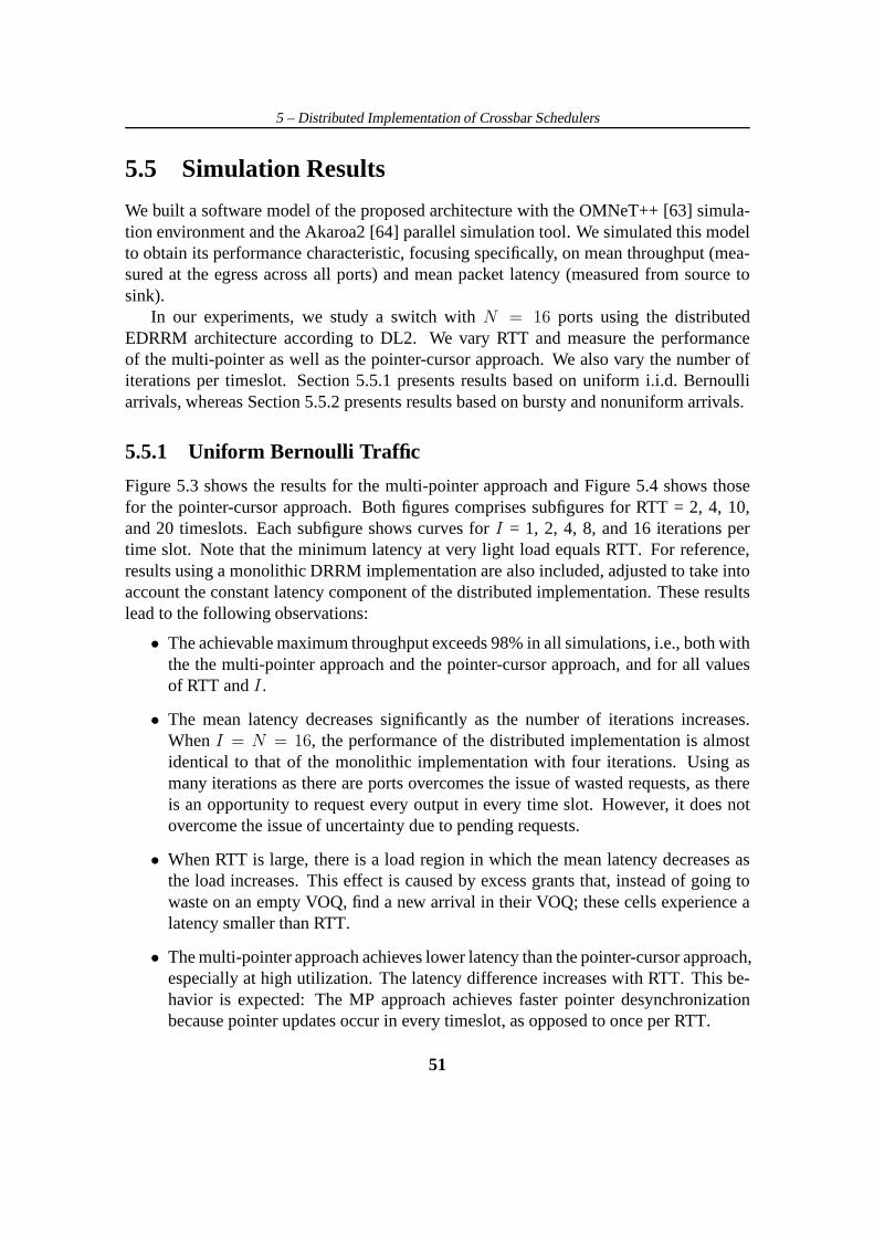
5 – Distributed Implementation of Crossbar Schedulers
5.5 Simulation Results
We built a software model of the proposed architecture with the OMNeT++ [63] simula-tion environment and the Akaroa2 [64] parallel simulation tool. We simulated this modelto obtain its performance characteristic, focusing specifically, on mean throughput (mea-sured at the egress across all ports) and mean packet latency(measured from source tosink).
In our experiments, we study a switch withN = 16 ports using the distributedEDRRM architecture according to DL2. We vary RTT and measurethe performanceof the multi-pointer as well as the pointer-cursor approach. We also vary the number ofiterations per timeslot. Section 5.5.1 presents results based on uniform i.i.d. Bernoulliarrivals, whereas Section 5.5.2 presents results based on bursty and nonuniform arrivals.
5.5.1 Uniform Bernoulli Traffic
Figure 5.3 shows the results for the multi-pointer approachand Figure 5.4 shows thosefor the pointer-cursor approach. Both figures comprises subfigures for RTT = 2, 4, 10,and 20 timeslots. Each subfigure shows curves forI = 1, 2, 4, 8, and 16 iterations pertime slot. Note that the minimum latency at very light load equals RTT. For reference,results using a monolithic DRRM implementation are also included, adjusted to take intoaccount the constant latency component of the distributed implementation. These resultslead to the following observations:
• The achievable maximum throughput exceeds 98% in all simulations, i.e., both withthe the multi-pointer approach and the pointer-cursor approach, and for all valuesof RTT andI.
• The mean latency decreases significantly as the number of iterations increases.WhenI = N = 16, the performance of the distributed implementation is almostidentical to that of the monolithic implementation with four iterations. Using asmany iterations as there are ports overcomes the issue of wasted requests, as thereis an opportunity to request every output in every time slot.However, it does notovercome the issue of uncertainty due to pending requests.
• When RTT is large, there is a load region in which the mean latency decreases asthe load increases. This effect is caused by excess grants that, instead of going towaste on an empty VOQ, find a new arrival in their VOQ; these cells experience alatency smaller than RTT.
• The multi-pointer approach achieves lower latency than thepointer-cursor approach,especially at high utilization. The latency difference increases with RTT. This be-havior is expected: The MP approach achieves faster pointerdesynchronizationbecause pointer updates occur in every timeslot, as opposedto once per RTT.
51

5 – Distributed Implementation of Crossbar Schedulers
512
256
128
64
32
16
8
4
2
1 0 0.1 0.2 0.3 0.4 0.5 0.6 0.7 0.8 0.9 1
Late
ncy
[tim
e sl
ots]
Throughput
I = 1I = 2I = 3I = 4I = 8
I = 16
(a) RTT= 2
512
256
128
64
32
16
8
4
2
1 0 0.1 0.2 0.3 0.4 0.5 0.6 0.7 0.8 0.9 1
Late
ncy
[tim
e sl
ots]
Throughput
I = 1I = 2I = 3I = 4I = 8
I = 16
(b) RTT = 4
512
256
128
64
32
16
8
4
2
1 0 0.1 0.2 0.3 0.4 0.5 0.6 0.7 0.8 0.9 1
Late
ncy
[tim
e sl
ots]
Throughput
I = 1I = 2I = 3I = 4I = 8
I = 16
(c) RTT = 10
512
256
128
64
32
16
8
4
2
1 0 0.1 0.2 0.3 0.4 0.5 0.6 0.7 0.8 0.9 1
Late
ncy
[tim
e sl
ots]
Throughput
I = 1I = 2I = 3I = 4I = 8
I = 16
(d) RTT = 20
Figure 5.3. Delay vs. throughput curves for the multi-pointer approach with varyingRTT.
Figure 5.5c shows the results for the multi-pointer approach with I = 1 and 4, anddemonstrates the impact of RTT. Here, the mean latency is normalized with respect toRTT. These curves clearly show that, in a limited load range,the mean latency dropsbelow RTT timeslots when RTT is large andI = 4.
Figure 5.6 compares the performance of the multi-pointer approachwith (Figure 5.6b)andwithout (Figure 5.6a) pending request counters withN = 16 and RTT= 4. Thesegraphs clearly show that use of PRCs achieves drastically lower latency throughout theload range. Considering the caseI = 1, the main difference is in the load range from10% to 70%; beyond 70% there is no noticeable latency difference. The reason is that,with heavy loads, the rate of wasted grants will be low, as most VOQs will be backlogged;therefore, the negative effect of excess requests is not noticed. At low to medium loads,on the other hand, many of the excess requests will result in wasted grants; every wastedgrant potentially is a wasted opportunity to transmit another cell, which therefore incursa longer latency. As a result, the mean latency increases. With I = 16, performance is
52

5 – Distributed Implementation of Crossbar Schedulers
2048
1024
512
256
128
64
32
16
8
4
2
1 0 0.1 0.2 0.3 0.4 0.5 0.6 0.7 0.8 0.9 1
Late
ncy
[tim
e sl
ots]
Throughput
I = 1I = 2I = 3I = 4I = 8
I = 16
(a) RTT= 2
2048
1024
512
256
128
64
32
16
8
4
2
1 0 0.1 0.2 0.3 0.4 0.5 0.6 0.7 0.8 0.9 1
Late
ncy
[tim
e sl
ots]
Throughput
I = 1I = 2I = 3I = 4I = 8
I = 16
(b) RTT = 4
2048
1024
512
256
128
64
32
16
8
4
2
1 0 0.1 0.2 0.3 0.4 0.5 0.6 0.7 0.8 0.9 1
Late
ncy
[tim
e sl
ots]
Throughput
I = 1I = 2I = 3I = 4I = 8
I = 16
(c) RTT = 10
2048
1024
512
256
128
64
32
16
8
4
2
1 0 0.1 0.2 0.3 0.4 0.5 0.6 0.7 0.8 0.9 1
Late
ncy
[tim
e sl
ots]
Throughput
I = 1I = 2I = 3I = 4I = 8
I = 16
(d) RTT = 20
Figure 5.4. Delay vs. throughput curves for the pointer-cursor approach with varyingRTT.
512
256
128
64
32
16
8
4
2 0 0.1 0.2 0.3 0.4 0.5 0.6 0.7 0.8 0.9 1
Late
ncy
[tim
e sl
ots]
Throughput
multi-pointer, I = 1multi-pointer, I = 4
multi-pointer, I = 16pointer-cursor, I = 1pointer-cursor, I = 4
pointer-cursor, I = 16monolithic DRRM, I = 4
(a) Delay vs. throughput compar-ison of both approaches, RTT=4
2048
1024
512
256
128
64
32
16
8 0 0.1 0.2 0.3 0.4 0.5 0.6 0.7 0.8 0.9 1
Late
ncy
[tim
e sl
ots]
Throughput
multi-pointer, I = 1multi-pointer, I = 4
multi-pointer, I = 16pointer-cursor, I = 1pointer-cursor, I = 4
pointer-cursor, I = 16monolithic DRRM, I = 4
(b) Delay vs. throughput compar-ison of both approaches, RTT=20
128
64
32
16
8
4
2
1
0.5 0 0.1 0.2 0.3 0.4 0.5 0.6 0.7 0.8 0.9 1
Late
ncy
[RT
T]
Throughput
I = 1, RT = 2I = 1, RT = 4
I = 1, RT = 10I = 1, RT = 20
I = 4, RT = 2I = 4, RT = 4
I = 4, RT = 10I = 4, RT = 20
(c) Normalized delay vs. through-put curves for the multi-pointerapproach with varying RTT.
Figure 5.5. Comparative figures.
close to ideal when using PRCs.
53

5 – Distributed Implementation of Crossbar Schedulers
256
128
64
32
16
8 0 0.1 0.2 0.3 0.4 0.5 0.6 0.7 0.8 0.9 1
Late
ncy
[tim
e sl
ots]
Throughput
distr-flppr-n16-multiptr-noprc.eps
distributed, I = 1distributed, I = 2distributed, I = 3distributed, I = 4distributed, I = 8
distributed, I = 16monolithic, I = 4
(a) Without PRCs
256
128
64
32
16
8 0 0.1 0.2 0.3 0.4 0.5 0.6 0.7 0.8 0.9 1
Late
ncy
[tim
e sl
ots]
Throughput
distr-flppr-n16-multiptr6.eps
distributed, I = 1distributed, I = 2distributed, I = 3distributed, I = 4distributed, I = 6distributed, I = 8
distributed, I = 16monolithic, I = 4
(b) With PRCs
Figure 5.6. Delay vs. throughput curves for the multi-pointer approach with RTT= 4,comparing performance with and without pending request counters.
5.5.2 Bursty and Nonuniform Traffic
To study the performance under nonuniform traffic, we adopt adestination distributioncharacterized by a non-uniformity parameterw [65], wherew = 0 corresponds to uniformtraffic andw = 1 to fully unbalanced, contention-free traffic:λij = λ
(w + 1−w
N
)if
i = j, λ1−wN
otherwise. Here,λij represents the traffic intensity from inputi to outputj,0 ≤ i,j < N ; λ is the aggregate offered load, andw the non-uniformity factor. Note thatno input or output is oversubscribed and that traffic is admissible as long asλ ≤ 1. Wevary the value ofw from 0 to 1 and measure the throughput achieved at an offered load of100%.
Figures 5.7(a,b) show the results forN = 16, RTT = 4, and Bernoulli arrivals forI ranging from 1 to 16. Also included for reference is a curve for monolithic DRRMwith I = 4. All curves exhibit the behavior of dipping to significantlyless than 100%throughput asw moves away from the extremes. However, increasingI increases thethroughput. The multi-pointer approach is able to reduce the gap with the reference tobelow four percentage points whenI ≥ 8. Overall, we again observe that the multi-pointer approach performance better than the pointer-cursor approach, with a differencein throughput that is generally less than five percentage points.
We also evaluate the performance using bursty traffic with geometrically distributedburst sizes with average burst size of 10 cells. Figure 5.8 shows the results. Here, wefirst observe that the maximum throughput again exceeds 98% in all cases. Moreover,the latency differences with the reference curves are even smaller than with Bernoullitraffic and the difference between the multi-pointer and pointer-cursor approaches is alsosignificantly smaller. Hence, the proposed distributed implementation is able to closelyapproximate a monolithic implementation in terms of performance for correlated as wellas uncorrelated arrivals.
54

5 – Distributed Implementation of Crossbar Schedulers
0.5
0.55
0.6
0.65
0.7
0.75
0.8
0.85
0.9
0.95
1
0 0.1 0.2 0.3 0.4 0.5 0.6 0.7 0.8 0.9 1
Thr
ough
put
Nonuniformity (w)
distributed, I = 1distributed, I = 2distributed, I = 3distributed, I = 4distributed, I = 8
distributed, I = 16monolithic, I = 4
(a) Multi-pointer
0.5
0.55
0.6
0.65
0.7
0.75
0.8
0.85
0.9
0.95
1
0 0.1 0.2 0.3 0.4 0.5 0.6 0.7 0.8 0.9 1
Thr
ough
put
Nonuniformity (w)
distributed, I = 1distributed, I = 2distributed, I = 3distributed, I = 4distributed, I = 8
distributed, I = 16monolithic, I = 4
(b) Pointer-cursor
Figure 5.7. Throughput vs. non-uniformity curves for both approaches withN = 16 andRTT = 4.
8192
4096
2048
1024
512
256
128
64
32
16
8
4 0 0.1 0.2 0.3 0.4 0.5 0.6 0.7 0.8 0.9 1
Throughput
distributed, I = 1distributed, I = 2distributed, I = 3distributed, I = 4distributed, I = 8
distributed, I = 16
(a) Multi-pointer
8192
4096
2048
1024
512
256
128
64
32
16
8
4 0 0.1 0.2 0.3 0.4 0.5 0.6 0.7 0.8 0.9 1
Throughput
distributed, I = 1distributed, I = 2distributed, I = 3distributed, I = 4distributed, I = 8
distributed, I = 16
(b) Pointer-cursor
8192
4096
2048
1024
512
256
128
64
32
16
8
4 0 0.1 0.2 0.3 0.4 0.5 0.6 0.7 0.8 0.9 1
Throughput
multi-pointer, I = 1multi-pointer, I = 4
multi-pointer, I = 16pointer-cursor, I = 1pointer-cursor, I = 4
pointer-cursor, I = 16monolithic, I = 4
(c) Comparison
Figure 5.8. Delay vs. throughput curves using bursty trafficfor both approaches withN = 16 and RTT= 4.
55

Chapter 6
Fair Integrated Scheduling of Unicastand Multicast Traffic in Input-QueuedSwitches
In this chapter we present a scheme to concurrently scheduleunicast and multicast trafficin an input-queued switch. It aims at providing high performance under any mix of the twotraffic types as well as avoiding starvation of any connection. The key idea is to schedulethe two traffic types independently and in parallel and then arbitrate among them foraccess to the switching fabric. Unicast and multicast matching are combined in a singleintegrated one. The edges that are excluded from the integrated matching are guaranteedto receive service at a later time, thus preventing starvation. We use simulation to evaluatethe performance of a system employing the proposed scheme and show that, despite itssimplicity, it achieves the intended goals. We also design an enhanced remainder-servicepolicy to achieve better integration and further improve performance.
This work was performed in the context of the OSMOSIS project(Chapter 4), but isgenerally applicable to input-queued crossbar-based synchronous switches.
6.1 Motivation
In environments where packet switches are used (TCP/IP networks, Storage Area Net-works, supercomputer interconnects) the vast majority of traffic consists of unicast (point-to-point) connections. However, in all these contexts, support for multicast (point-to-multipoint) traffic is essential. On the Internet, multicast enables applications such asaudio- and video-conferencing, multimedia content distribution (radio, TV) and remote
56

6 – Fair Integrated Scheduling of Unicast and Multicast Traffic in Input-Queued Switches
collaboration; in SANs, it is required to replicate data among multiple sites or to dis-tribute content to multiple servers; in supercomputing architectures it is essential to im-plement cache coherency protocols and support collective operations [40]. Ideally, a net-work switch should be able to achieve high performance underany mix of the two traffictypes.
Multicast packets can be treated as unicast simply by sending a separate copy of thepacket to each of the intended destinations; conversely, unicast packets can be consideredas multicast packets with only one destination and treated without any differentiation.These trivial solutions allow the switch to handle both types of traffic concurrently but arefar from optimal and generally lead to poor performance.
Another issue to address when both unicast and multicast arepresent is fairness. Atraffic type must not be allowed to monopolize switch resources; however, it is also im-portant to guarantee thatall connections of a given traffic type receive service. When bothconditions are met, we say that the switch scheduler isfair.
In this work we propose a novel method for integrated scheduling of unicast andmulticast traffic. It leads to high utilization of switch resources under any traffic mix,guarantees fairness, and exhibits a number of other desirable properties.
Although the problem of supporting unicast and multicast concurrently is clearly im-portant, not much attention has been devoted to it in the past. The problem has beenthoroughly studied from a theoretical point of view in [66] and its hardness has beenassessed. These authors also propose an integration schemethat consists of schedulingmulticast first and using the remaining resources for unicast. This scheme, which we call“sequential” predictably leads to high performance because it uses the switch resourcesvery efficiently. The multicast scheduler has all the resources at its disposal and canproduce its best matching. The unicast scheduler, on the contrary, is constrained by theremaining resources but, thanks to the VOQs, it can fully exploit them and increase thesize of the total matching. The main disadvantage of this scheme is that it easily leads tostarvation of unicast traffic. A single input loading the switch with broadcast traffic wouldsuffice to prevent unicast from getting any service at all. In[67] the authors propose a re-finement of the sequential scheme, in which at some timeslotsthe unicast scheduler runsfirst while in other the multicast scheduler is given priority. The choice of which schedulerruns first in a given interval, however, is based on a parameter that depends on the trafficpatterns, in particular on the ratio of multicast to unicasttraffic, and that must be deter-mined a-priori to guarantee high performance. Smiljanic showed that a practical approachto achieve integrated scheduling is to treat multicast traffic as unicast, but distributing theburden of cell replication over multiple ports [68]. The main problem with this schemeis that it potentially introduces very high latency, so it isnot suitable for our applications.The problem was also considered in [69], but the proposed solution is mainly targeted toshared-memory switches.
57

6 – Fair Integrated Scheduling of Unicast and Multicast Traffic in Input-Queued Switches
VOQ
VOQ
MC−Q
N−1
0
VOQ
VOQ
MC−Q
N−1
0
Req. Grants
MC Sched.UC Sched.
Integrated Scheduler
Crossbarconfig
Input (N−1)
Input 0
Crossbar
Output 0
Output (N−1)
Figure 6.1. Reference architecture
6.2 Fair Integrated Scheduling
Our integration scheme is conceived for a synchronous, IQ, crossbar-based,N×N switch(Figure 6.1). The scheme is independent from the queueing structure adopted for unicastor multicast traffic, but for concreteness we refer to the most common situation in whicheach switch input maintainsN VOQs for unicast and a single FIFO queue for multicast.
6.2.1 Reference architecture
At every timeslot, contentions among the cells of a single traffic type are resolved sepa-rately by specialized schedulers. The unicast scheduler receives requests from the inputsfor non-empty VOQs and produces a one-to-one matching between the inputs and theoutputs. The multicast scheduler examines the fanout of thecells that are at the HOL ofthe multicast queues and produces a one-to-many matching. Fanout splitting is allowed:during a timeslot a multicast cell can receive partial service, being transmitted only to asubset of its destinations.
As the two schedulers run in parallel and independently, thematchings they produce ingeneral are overlapping, meaning that they have conflictingedges. To obtain a consistentconfiguration for the crossbar, the two matchings must be combined into a single one. Anintegration blockdecides which unicast and multicast edges will be part of theintegratedmatching. The set of edges that are excluded from the integrated matching is called theremainder.
The request filteris a block capable of reserving a subset of the switch inputs andoutputs by dropping the corresponding unicast and multicast requests. Reservations at
58

6 – Fair Integrated Scheduling of Unicast and Multicast Traffic in Input-Queued Switches
Sched.Multicast
Multicast
Requests
Requests
Unicast
Integrated
Matching
UnicastSched.
Req.Filter
Integr.Block
Remainder
MC Matching
UC Matching
Figure 6.2. The FILM integration scheme
any timeslot may be made on the basis of information providedby a number of sources,including current requests and the integration block.
Employing two different schedulers that run in parallel provides important advantages.The designer is free to choose the algorithms that better fit his or her needs. The systemcan easily be partitioned over multiple chips. The minimum timeslot duration is deter-mined by the scheduling time of the slowest scheduler, whereas, if the schedulers ran insequence, it would be limited by the sum of the two.1 Moreover, it avoids the additionallatency naturally introduced by sequential schemes.
A block diagram of this scheme, called “FILM” (FILter & Merge), is shown in Fig-ure 6.2.
6.2.2 Achieving fairness
In the FILM scheme each connection goes through two points ofcontention: first it com-petes with the other connections belonging to the same traffic type, then with those of theother traffic type. To achieve fairness we must make sure thatevery connection regularlyhas a chance to win both contentions.
A scheduling algorithm is starvation-free if it guaranteesthat no queue is allowed toremain unserved indefinitely. As this is a fundamental property, many algorithms ex-hibit it. Unicast algorithms such asi-SLIP [19] and DRRM [20] prevent starvation byusing pointers that keep track of which VOQs have been servedmost recently. Multi-cast algorithms, on the other hand, often take into account the age of a cell or the orderin which cells at different inputs have advanced to the HOL oftheir queues (e.g. WBAand TATRA [34], respectively). We require both schedulers to employ starvation-freealgorithms to be sure that all connections eventually get past the first contention point.
1We assume that the delay contributed by the additional blocks is much lower than the scheduling times.As we will see in Section6.5 devoted to implementation complexity, this assumption is likely to hold.
59

6 – Fair Integrated Scheduling of Unicast and Multicast Traffic in Input-Queued Switches
Connections that have been selected by their schedulers still remain unserved if theintegration block excludes them from the integrated matching. The scheduler is unawareof the fact that granted service has in fact been withdrawn, so fairness is no longer guaran-teed. A solution to this problem is to make sure that all edgesthat are part of the remainderactually receive service, albeit in a later timeslot.
6.2.3 Integration policy
The performance of multicast scheduling algorithms variesconsiderably, as demonstratedin [34]. This is due to the fact that the single FIFO queuing architecture causes HOLblocking, therefore the algorithms must carefully choose which inputs to serve in orderto mitigate its effects. For example, it is shown that “concentrating the residue” at ev-ery timeslot (which roughly means providing full service toas many inputs as possible)greatly helps in draining the queues fast. Hence, special care should be taken when ma-nipulating multicast matchings to avoid compromising the effectiveness of the choicesmade by the scheduler.
Unicast scheduling, on the contrary, is less sensitive to withdrawal of resources be-cause the VOQs provide the scheduler with a wide choice of connections to serve. More-over it is important to note that if unicast and multicast contend for an input, only oneedge is lost if multicast wins, whereas multiple edges mightbe removed if it loses.
Following these considerations, we opt for an integration policy that gives strict prior-ity to multicast over unicast. Hence, the algorithm implemented in the integration blockcan be formulated as follows:
1. Start with an empty matching,
2. add all multicast edges,
3. add all non-conflicting unicast edges.
As a consequence, the remainder always contains only unicast edges.
6.2.4 Remainder-service policy
As noted above, if a remainder is produced in a timeslot, it isimportant to ensure thatall the edges it contains are eventually served. This can be done according to differentpolicies, the simplest one being to serve all of them in the next timeslot. As these edgesare part of a matching, they do not conflict with each other. Inaddition, the resources theyclaim are known and can be reserved to avoid further contention.
At every timeslot, new unicast and multicast requests are issued. The request filterdrops all those that involve inputs and outputs needed to serve the remainder produced
60

6 – Fair Integrated Scheduling of Unicast and Multicast Traffic in Input-Queued Switches
in the preceding timeslot and submits the others to the corresponding scheduler. Accord-ingly, the integration block issues grants for the edges in the remainder and for those inthe current matching. A new remainder is produced and fed back to the request filter forthe next timeslot.
An important property of the scheme is that, as a consequenceof filtering unicastrequests, the remainders produced in two consecutive timeslots are disjoint, i.e., haveno inputs or outputs in common. This is crucial for fairness because it assures that allswitch resources eventually become available for scheduling. Reserving resources for theremainder does not persistently preclude access to any input or output.
We expect this combination of integration and remainder-service policy to achievegood link utilization. The resources allocated to the remainder are fully utilized and thoseremaining can be assigned either to unicast or multicast. The integration block preservesthe matching produced by the multicast scheduler, but triesto enlarge it by adding unicastedges.
6.3 Simulation Results
We have studied the performance of a system employing the FILM scheme by simula-tion. In particular, we observed the total throughput as well as the individual throughputsof unicast and multicast traffic as the fraction of multicasttraffic (MCF) grows from0(unicast only) to1 (multicast only). Ideally, the throughput achieved by eachtraffic typeshould be equal to the corresponding share of the output loadand the total should be100%.
The simulated system is an8×8 switch with infinite buffers at the inputs. The unicastscheduler usesi-SLIP with three iterations and the multicast scheduler uses WBA. Sim-ulations run for 1 million cell times and results are collected after a quarter of the totalsimulation time has elapsed.
Cells are generated according to an i.i.d. Bernoulli process, i.e. every input portreceives a cell with probabilityρ, equal to the input load. Each cell has a probabilityPof being a multicast cell. The fanout of multicast cells is uniformly distributed between 2and 8. Traffic is uniform, i.e. all outputs have the same probability of being the destinationof a unicast cell or of belonging to the fanout of a multicast cell. Note that, under theseconditions and with this choice of scheduling algorithms, when the switch is loaded onlywith multicast traffic, the maximum throughput it can achieve is approximately0.93 [34],whereas it is1.0 when only unicast is present.
The total load on the switch isρ(PF + (1 − P )) whereF is the average fanout. Inour case,F = 5 andP andρ are varied to obtain the desired multicast load on the switchwhile keeping the total load equal to 1.
61

6 – Fair Integrated Scheduling of Unicast and Multicast Traffic in Input-Queued Switches
0
0.1
0.2
0.3
0.4
0.5
0.6
0.7
0.8
0.9
1
0 0.1 0.2 0.3 0.4 0.5 0.6 0.7 0.8 0.9 1
Thr
ough
put
Fraction of Multicast Traffic
FILM, totalFILM, UnicastFILM, Multicast
Sequential, totalSequential, UnicastSequential, Multicast
Figure 6.3. Performance of the FILM integration scheme
Figure 6.3 shows the throughput achieved by FILM with the integration and remainder-service policies described in the preceding section. The performance of the sequentialscheme, which is close to ideal, is also shown for reference.
The total throughput achieved by our scheme is always higherthan 0.9. Unicastthroughput shows very little degradation (on the order of a few percent) when it is thepredominant traffic type, whereas it achieves ideal performance when multicast is pre-dominant. However, multicast throughput progressively decreases with respect to outputload as MCF grows from0.4 to 1.0. The worst case is MCF= 0.7, when multicastthroughput is0.6 instead of0.7. This also corresponds to the point at which the overallthroughput is at its minimum (0.9).
Figure 6.4 shows the delay experienced by unicast and multicast cells as a function ofthe throughput when MCF= 0.5, i.e., when each traffic type is responsible for half of theoutput load. The unicast curve is bounded for any value of thetotal throughput, whereasthe multicast curve saturates when it approaches1.0.
6.4 Enhanced Remainder-Service Policy
Although the scheme presented above provides overall good performance and is quitesimple, it has a drawback: it penalizes multicast traffic most, especially when it is pre-dominant.
Multicast performance is limited because at every timeslot, some switch resources areused to discharge the remainder. Although it is essential toeventually serve all edges
62

6 – Fair Integrated Scheduling of Unicast and Multicast Traffic in Input-Queued Switches
1
10
100
1000
0.1 0.2 0.3 0.4 0.5 0.6 0.7 0.8 0.9 1
Del
ay
Throughput
AverageUnicast
Multicast
Figure 6.4. Delay vs. throughput curves for the FILM integration scheme
that are not selected in the merge, it is not necessary to do soimmediately. Thanks tothe disjoint remainder property, it is possible toaccumulatethe remainders producedin consecutive timeslots and serve the individual edges when the conditions are mostfavorable. The remainder-service policy identifies which edges should be served at everytimeslot and filters the corresponding multicast requests.Unicast requests, in contrast, arealways filtered using all the accumulated edges to obtain disjoint remainders.
A good policy should be able to serve the edges in the remainder rapidly and at thesame time cause as little disruption as possible to the flow ofmulticast cells. We proposeanenhancedpolicy that serves a remainder edge if it uses
1. an input not requested by multicast OR
2. an output not requested by multicast OR
3. an input that discharged a multicast cell in the precedingtimeslot.
The first two rules obviously aim at improving integration: if it is possible to use a re-source that would otherwise remain idle, it is desirable to do so. In this case the costof serving a remainder edge is to make one output (first rule) or one input (second rule)unavailable to multicast.
The third rule instead stems from the general observations on multicast schedulingfound in [34]. The scheduler tends to favor cells that contend with few others. Cells thathave just advanced to the HOL still have their full, usually large, fanout and cause manyconflicts. They are unlikely to receive much consideration,so postponing their scheduling
63

6 – Fair Integrated Scheduling of Unicast and Multicast Traffic in Input-Queued Switches
0
0.1
0.2
0.3
0.4
0.5
0.6
0.7
0.8
0.9
1
0 0.1 0.2 0.3 0.4 0.5 0.6 0.7 0.8 0.9 1
Thr
ough
put
Fraction of Multicast Traffic
Enh. FILM, totalEnh. FILM, UnicastEnh. FILM, Multicast
Base FILM, totalBase FILM, UnicastBase FILM, Multicast
Figure 6.5. Performance of FILM with enhanced remainder-service policy
should not significantly affect the quality of the matching.This rule is particularly impor-tant because it enables fairness: the multicast scheduler guarantees that the HOL cell atany input will be served in finite time; consequently, the inputs becomes available to serveremainder edges. Many algorithms (such as TATRA, WBA and mRRM [70]) ensure thatat least one multicast cell is fully discharged at every timeslot.
Figure 6.5 shows the performance of FILM when the enhanced policy is used, un-der the same conditions as in Section 6.3. The benefits on multicast traffic are evident:throughput is increased when(0.4 < MCF < 0.9) and closely tracks the output load upto MCF = 0.7. Unicast, on the other hand, shows a moderate decrease in thesame range.In the worst case (MCF= 0.7), the difference with respect to the output load is slightlylower than0.06. Overall throughput is noticeably increased when multicast predominates,whereas it shows little degradation when both traffic types are equally active.
Figure 6.6 shows the delay vs. throughput curve for this situation. Multicast experi-ences very low delay, seeming to be almost insensitive to thepresence of unicast. Unicastdelay instead saturates when the total throughput is approximately0.95.
6.5 Implementation Complexity
In this section we discuss some implementation aspects of the FILM scheme in order toget an idea of its complexity.
64
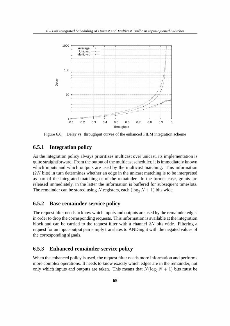
6 – Fair Integrated Scheduling of Unicast and Multicast Traffic in Input-Queued Switches
1
10
100
1000
0.1 0.2 0.3 0.4 0.5 0.6 0.7 0.8 0.9 1
Del
ay
Throughput
AverageUnicast
Multicast
Figure 6.6. Delay vs. throughput curves of the enhanced FILMintegration scheme
6.5.1 Integration policy
As the integration policy always prioritizes multicast over unicast, its implementation isquite straightforward. From the output of the multicast scheduler, it is immediately knownwhich inputs and which outputs are used by the multicast matching. This information(2N bits) in turn determines whether an edge in the unicast matching is to be interpretedas part of the integrated matching or of the remainder. In theformer case, grants arereleased immediately, in the latter the information is buffered for subsequent timeslots.The remainder can be stored usingN registers, each(log2 N + 1) bits wide.
6.5.2 Base remainder-service policy
The request filter needs to know which inputs and outputs are used by the remainder edgesin order to drop the corresponding requests. This information is available at the integrationblock and can be carried to the request filter with a channel2N bits wide. Filtering arequest for an input-output pair simply translates to ANDing it with the negated values ofthe corresponding signals.
6.5.3 Enhanced remainder-service policy
When the enhanced policy is used, the request filter needs more information and performsmore complex operations. It needs to know exactly which edges are in the remainder, notonly which inputs and outputs are taken. This means thatN(log
2N + 1) bits must be
65

6 – Fair Integrated Scheduling of Unicast and Multicast Traffic in Input-Queued Switches
transferred from the integration block. The information about which inputs dischargeda multicast cell in the preceding timeslot consists ofN bits and can be maintained bythe queues managers. Finally, the information about which inputs and which outputs arebeing requested by multicast (2N bits) is readily available as it can be derived from therequests themselves.
Unicast requests are filtered using all edges in the remainder as in the previous case,whereas multicast requests are filtered depending on which remainder edges are served.This information is produced at the request filter block by ORing the signals correspond-ing to the three conditions that grant service to an edge. Theintegration block also needsto know which edges are served, as it has to issue the appropriate grants. As the remainderedges are part of a matching, onlyN bits need to be transferred from the request filter tothe integration block.
As a final remark, we wish to highlight that all the operationsdescribed above can beperformed in parallel and implemented using combinationallogic only.
66
Chapter 7
Conclusions – Part I
In the first part of this thesis we have discussed the design ofpacket switches for super-computer interconnection networks.
We have started with an overview of supercomputing systems,illustrating how vari-ous factors such as the node architecture, the partitioningof the memory space and theprogramming model influence the requirements of the interconnection network. We haveexplained why optical switching has the potential to be the best technology to satisfy thedemanding requirements of supercomputers and which factors limit its deployment.
We have then introduced OSMOSIS, a research project jointlydeveloped by IBM andCorning that aims at building a demonstrator interconnect for HPC applications. Thebuilding block of the interconnect is a hybrid switch with anall-optical data-path and anelectronic control-path. The switch is designed to meet an ambitious set of requirementsthat include very low latency, high throughput, high port count, high line rate, scalabilityto thousands of ports and efficient support of multicast traffic. The design of the control-path is further complicated by the need to use only FPGAs.
In the context of the OSMOSIS project we have the developed techniques that enablethe construction of multi-chip crossbar schedulers, whichconstitute the first contributionof this part of the thesis. These techniques overcome the area, pin-count and power densityconstraints of single-chip schedulers and thus allow scheduling of much larger crossbarsthan previously possible. The distribution techniques we have proposed can be appliedto various parallel iterative matching algorithms, such asDRRM and SLIP, and preservetheir throughput and fairness properties. The first, namedmulti-pointer, is based on du-plication of status information and the performance it provides is almost insensitive to theRTT between chips. The second one is calledpointer-cursor, is based on heuristic updateof status information and has constant complexity; performance, however, degrades asthe RTT grows. Simulation results show that high performance levels are maintained un-der uniform i.i.d. traffic, even when the scheduler is distributed over2N chips separatedby distances equivalent to several time slots. Moreover, with proper distribution level
67

7 – Conclusions – Part I
and number of iteration, satisfactory performance is achieved also under non-uniform andbursty traffic.
We then devoted our attention to the problem of scheduling concurrently unicastand multicast traffic in an input-queued switch. We have developed a novel integrationscheme, named FILM, capable of scheduling the two traffic types fairly and efficiently,without a-priori knowledge of traffic characteristics. Thescheme first schedules the twotraffic types separately and then arbitrates among the results for access to the switchingfabric. A integration block combines the matchings produced by the two schedulers, pro-ducing an integrated matching and a remainder. The remainder contains edges that cannotbe served in the current time slot, but are guaranteed to receive service in a subsequentone. The first remainder service policy we have proposed is extremely simple and per-forms well, but tends to penalize multicast. The second one is more sophisticated and isable to minimize the interference with the flow of multicast cells. It leads to a very highoverall performance and an almost ideal treatment of multicast traffic, at the cost of someadditional complexity.
Although the work described in this part of the thesis has been performed to specifi-cally address the challenges posed by the design of the OSMOSIS scheduler, we believethat it is valuable in all the contexts in which high-performance packet switches are used.
68

Part II
A Switching Architecture forStorage Area Networks

Chapter 8
Introduction to Storage Area Networks
Nowadays servers are at the center of the enterprise information system. They run mission-critical applications, such as enterprise resource planning (ERP), supply chain manage-ment and customer relationship management (CRM). With the advent of the Internet ande-business, servers are used to do on-line transaction processing (OLTP) and provide ser-vices to millions of users. They must be able to access data inthe storage subsystemquickly and reliably. Failure to do so directly translates to significant costs and loss ofrevenue.
In this chapter we describe the evolution of the I/O interface between servers andstorage devices, pointing out the limits of directly-attached storage and how storage net-working overcomes them. We then introduce Fibre Channel as the preferred networktechnology to implement a SAN and outline its most importantcharacteristics.
8.1 Limits of directly-attached storage
Computing nodes have been traditionally connected to theirstorage resources (disks,tapes, CD libraries, etc.) by means of a fixed, dedicated channel, such as the SCSI parallelbus.
In recent years this paradigm, called “Directly-attached Storage” (DAS) has becomeinadequate. As servers grow in number and request additional capacity, several differentproblems arise. The most important are:
• Scalability: the number of devices that can be attached to a disk controller is limitedto few tens. Even with multiple controllers in the same server, the total availablecapacity might be insufficient.
• Performance: as the physical media is shared, adding devices results in morearbitration overhead and less bandwidth being available toeach of them.
70

8 – Introduction to Storage Area Networks
• Distance limitations: parallel buses are limited in length to few tens of meters byelectrical issues, such as skew. Skew is a phenomenon typical of parallel transmis-sion. Electrical pulses transmitted on different line of the parallel bus do not reachthe target device at exactly the same time. If the delay between the first and thelast arriving pulse is comparable to the time slot occupied by the pulse itself, thereceiver cannot correctly decode the transmitted bit string.
• Availability: devices attached to the bus cannot be added or removed withoutputting the whole string off-line. This causes downtime every time the storagesubsystem needs to be reconfigured.
• Data protection: each server must be equipped with proper devices (for example,tape drives) to backup its data. With hundreds or even thousands of servers, thisis costly and quickly becomes an administrative burden, as each server must bebacked up separately. If backup operations are performed through the LAN, theperformance of the corporate network might be severely impacted for long timeframes.
• Efficiency: disk space not used by a server cannot be relocated to anotherone. Theadministrators may need to buy and install additional storage devices even if freespace exists on those already available.
A close look to the problems listed above suggests that many of them are intrinsic tothe DAS model and cannot be solved simply with technologicalenhancements.
8.2 Storage Area Networks
Storage Area Networks (SANs) have emerged as the key solution to address the perfor-mance, scalability, reliability and maintainability issues posed by DAS. The SAN is adedicated network infrastructure that provides meshed, any-to-any connectivity betweenservers and storage devices.
The introduction of networking concepts and technologies as a replacement of a sin-gle, direct connection, redefines the relationship betweenservers and storage devices andenables the design of new information systems, as depicted in Figure 8.1. Storage re-sources are now a separated and well-delimited component ofthe system and serversbecome the front-end towards the users.
This novel organization of storage resources enables the implementation of new paradigms,providing several benefits [71]:
• Storage consolidation:as servers are no-longer directly connected to disks, all thedisks can be physically relocated in one or more disk arrays.Disk arrays are devicesable to host tens or hundreds of disks. By using the management interface of the
71

8 – Introduction to Storage Area Networks
LAN / WAN
SAN
Clients
Servers
StorageDevices
Figure 8.1. An information system employing a SAN
disk array, the storage administrator can allocate to each server a proper fraction ofthe total capacity. Additional space can be provided without disruption by addingdisks to the array and reconfiguring it. Storage consolidation can take place evenacross multiple disk arrays.
• Remote replication and disaster recovery:data can be protected from disk faultsby using a technique called “mirroring”. A pool of physical disks of equal capacityis combined in a single, virtual disk of the same capacity. Data written to the virtualdisk is physically stored on all the disks in the pool. If any of the disks in thepool fail, data is immediately available on the others and the server can continue
72

8 – Introduction to Storage Area Networks
its operations without disruption. As a SAN can connect devices located tens ofKilometers away, data can be replicated on remote sites, providing protection evenin case of disasters, such as natural calamities or terrorist attacks.
• Server clustering: a cluster is a set of servers working concurrently on the sameset of data. Clustering provides higher performance (as theservers work in parallel)and higher reliability (if one of the server fails, it simplygoes out of the cluster).Although complex issues exist at the operating system and application level (inter-process communication, concurrent data access, etc.) a SANeffectively promotesclustering because it allows easy sharing of common data.
• LAN-free, server-free backup: data stored in multiple disk arrays can be backedup directly to large, shared tape drives, without traversing the LAN and withoutinvolving the servers. All operations are scheduled and managed from a single,central location.
• Storage resources management:the ability to have a consistent and unified viewof all the storage devices greatly simplifies monitoring andallocation of resources,as well as provisioning and planning.
In general, the deployment of a SAN enablesvirtualization, i.e. the capability to provideto computing nodes a logical view of available storage resources that is independent ofthe physical location and the specific characteristics of the devices.
8.3 Networking Technologies for SANs
SANs are networks in all respects and present all the features typical of networkingtechnologies. The most important characteristics inherited from the networking worldare:
• serial transport, to ship data over long distances at high rates
• data packetization, to achieve high link efficiency and fairsharing of network re-sources
• addressing schemes that support very large device population
• routing capabilities, to provide multiple, redundant paths between source and des-tination devices
• a layered architecture, to support the transport of different protocols at the upperlayers and the usage of different interfaces at the lower ones.
73

8 – Introduction to Storage Area Networks
SANs can be built using different networking technologies,however, it it is importantto remember that servers, operating systems and applications still expect from the storageinterface a “channel-like” behavior, i.e. high-speed, low-latency, error-free communi-cations. Networking technologies used to implement SANs must therefore be carefullychosen and deployed in order to satisfy these strict requirements.
Today the preferred networking technology for SANs is FibreChannel, although dif-ferent solutions such as iSCSI (based on TCP/IP and Ethernet[72]) or Infiniband [36]have been proposed.
8.3.1 Fibre Channel
Fibre Channel is a multi-purpose, standard-based networking technology, specifically de-signed for computing environments. Its design is based on the assumption that the trans-port media (copper cable or optical fiber) is reliable, henceerror recovery mechanisms arereduced to a minimum and are mostly left to upper layer protocols. Data are fragmentedand encapsulated in network protocols with minimum overhead, in order to achieve highefficiency. Intermediate nodes guarantee that frames will not be discarded, duplicatedor delivered out-of-order under any circumstances. A simple, credit-based mechanismis used for flow and congestion control. These characteristics of the data-path make afull hardware-based implementation feasible. Incoming frames can be processed by endnodes at very high speed and do not incur the latency induced by large reassembly andreordering buffers.
8.3.2 Credit-based flow control
Flow control mechanisms are used to regulate the rate at which a transmitter sends frames,in order to achieve efficient bandwidth utilization withoutoverwhelming the receiver.These mechanism represent one of the most important characteristics of a networkingtechnology and have a very strong influence on the design of network devices.
In Fibre Channel networks flow control mechanisms are based on the concept ofcredit. A credit represents the ability of a receiver to accommodate one frame. Thereceiver grants to the transmitter an initial number of credits, typically proportional to thesize of its buffers. The transmitter is authorized to send one frame for each credit it hasreceived; after that it has to stop until it receives more. Assoon as the receiver has finishedprocessing an incoming frame (for instance, it has passed itto upper layers) it can free theresources that were used by that frame and grant a new credit.
Fibre Channel provides two levels of flow control: “buffer-to-buffer” and “end-to-end”. Buffer-to-buffer flow control takes place between pairs of adjacent ports, such as alink between a node and a switch or between two switches. It operates on all the packetstraversing the link, without the capability to discriminate among multiple flows. End-to-end flow control, on the contrary, operates only between end-nodes and is performed per
74
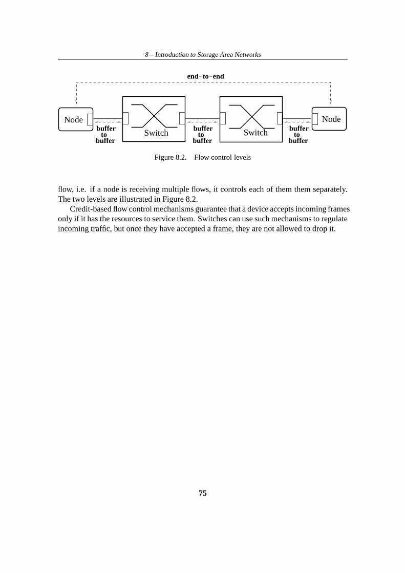
8 – Introduction to Storage Area Networks
Node Nodebuffer
tobuffer
bufferto
buffer
bufferto
bufferSwitch Switch
end−to−end
Figure 8.2. Flow control levels
flow, i.e. if a node is receiving multiple flows, it controls each of them them separately.The two levels are illustrated in Figure 8.2.
Credit-based flow control mechanisms guarantee that a device accepts incoming framesonly if it has the resources to service them. Switches can usesuch mechanisms to regulateincoming traffic, but once they have accepted a frame, they are not allowed to drop it.
75

Chapter 9
The Switching Architecture
In this chapter we present the architecture of a CIOQ switch specifically designed forFibre Channel SANs. The main differentiation points with respect to traditional LANswitches and Internet routers are the asynchronous design,the addition of a centralizedarbiter and the employment of a number of buffer management techniques that guaranteeloss-free operation. We first present the base architecture, considering unicast traffic only,and then discuss extensions to support multicast.
9.1 System Overview
The logical architecture of the system is depicted in Figure9.1. It is composed by aset ofNLC linecards interconnected by a crossbar-based switching fabric. Each linecardhostsPLC input/output ports and has two links to the switching fabric, nameduplinkand downlink. Packets enter the linecard through input ports and are multiplexed onthe uplink. They traverse the fabric and are transmitted to the proper output linecardon the downlink. After demultiplexing, they finally reach the destination output port.The bandwidth of the uplink and the downlink is equal to the sum of the bandwidths ofthe input/output ports hosted on a linecard, so they are not oversubscribed and do notconstitute a bottleneck.
The system is fully asynchronous, i.e. the linecards and theswitching fabric run onindependent clock domains. This feature provides several benefits in terms of simplicity,cost and scalability [4]. First, it prevents the necessity to maintain and distribute a globalclock signal, a task that can be problematic, especially if modules are distributed amongmultiple racks. Second, it enables native support for variable-length packets, eliminatingthe need for segmentation and reassembly buffers. Finally,it allows simplified arbitrationof the switching fabric, without employing complex scheduling algorithms. These advan-tages, however, come at a price: buffers are needed at the fabric inputs and outputs, andmoderate speed-up is required to achieve good performance.
76

9 – The Switching Architecture
output portsinput portsoutput portsinput ports
Packet StoreModule
Packet StoreModule
PLCP
LCP
LCPLC
Control Path
Data Path
Requestsand Grants
Arbiter
In−Module Out−ModuleOut−Module
Credits
In−Module
Switching Fabric
Line−CardLine−Card
Figure 9.1. Logical architecture of the switch, showing twolinecards
77

9 – The Switching Architecture
To achieve lossless operation, all buffers are endowed witha backpressuremecha-nism, that allows them to block transmission from previous stages when they are close tosaturation. The signal is activated when occupancy grows above a certain threshold andis deactivated when it decreases below another threshold.
This form of flow-control is sufficient to prevent buffer overflow, but is too coarse, asit does not discriminate among multiple flows traversing theswitch. Therefore the systememploys an additional centralized mechanism that guarantees fairness among multipleflows and enhances performance.
9.2 Data Path
9.2.1 Linecards
The Packet-Store Module (PSM) is a large buffer that stores packets entering on inputports1. Memory is divided in slots of equal size, dimensioned to contain a maximum-sizepacket2; if a smaller packet is stored, the remaining part of the slotis unusable. Memorysegmentation reduces usage efficiency but simplifies the implementation of buffer man-agement schemes. Total capacity is statically partitionedamong input ports. If the spaceassigned to a specific port is completely used, the port uses buffer-to-buffer flow control(Section 8.3.2) to inhibit transmission from the connectednode. Buffer space is logicallyorganized to provide a separate set of VOQs to each input port. Ports select independentlyand in parallel packets to be transferred to the In-module using a round-robin policy.
The In-module is a fast and small random-access memory, thatacts as a high-speedinterface towards the switching fabric. It contains a smallnumber of fixed-size slots,organized as a single set of VOQs. Access to the In-module memory is regulated bya buffer management mechanism that prevents input ports from monopolizing availablespace. Moreover, if a VOQ in the In-module grows beyond a specific size, no morepackets from the corresponding destination are accepted from the PSM VOQs. When allIn-module slots are occupied, a backpressure signal blocksany packet transfer from thePSM.
The Out-module receives from the switching fabric the aggregate flow of packets di-rected to the linecard and demultiplexes it based on the destination port. Memory issegmented in fixed-size slots and structured as a set ofPLC queues, one for each outputport on the linecard. Queues cannot overflow because space ispre-allocated using thecredit-based flow-control mechanism described in Section 9.3.1. The logical layout of alinecard, highlighting queueing stages, is shown in Figure9.2.
1In a practical implementation, PSM functionalities would be spread among multiple chips, each servinga subset of the input ports.
2MTU is 2 KB for Fibre Channel devices.
78

9 – The Switching Architecture
Q1 QN Q1 Q1 QN
QNQ2Q1
LC
NQ
Out−moduleIn−module
PSM
VOQs
Outp. 1 Outp. P
VOQs SetInput 1
VOQs SetInput 2
VOQs SetInput P
LCOutp. 2
Figure 9.2. Logical layout of a linecard
9.2.2 Switching fabric
The switching fabric is based on aNLC×NLC crossbar. As the fabric runs asynchronouslywith respect to the linecards, buffers are required at the input and outputfabric ports. Thesize of these buffers is determined by the Round-Trip Time (RTT) between the linecardsand the fabric. In principle, if the RTT is negligible, a single MTU-sized buffer suffices.In practice it is necessary to have more, to take into accountstore-and-forward delayand other sources of overhead that contribute to the RTT. Moreover, it is desirable tosupport multi-rack configurations, in which the RTT is largedue to propagation delay.The actual size of these buffers is chosen to be on the order offew tens of MTUs per port,depending on the constraints imposed by chip technology. Packets are stored contiguouslyin memory (i.e. there is no segmentation) to maximize efficiency. Buffer overflow isprevented using a backpressure signal that blocks transmission from the linecard whenspace is exhausted.
As the available amount of memory is small and the clock frequency high, it is notpossible to implement VOQs at the fabric input ports. Each input buffer is organized as asingle FIFO queue, hence the fabric suffers from HOL-blocking. This phenomenon canseverely impact throughput [8] but its effects can be partially mitigated by providing amoderate speed-upK.
Buffers at the fabric output ports receive packets atK times the rate of fabric inputports, so they must be able to store at leastK MTUs. In order to sustain temporary
79

9 – The Switching Architecture
overload conditions, their size is chosen to beK times the size of the input buffers.At the head of multiple fabric input queues there might be packets directed to the
same linecard. Each crossbar output can receive packets from only one crossbar input ata time, hence arbitration is necessary to resolve the contention. This task is performed bysimplefabric arbiters, one for each crossbar output, that select a crossbar input amongthe contending ones in a round-robin fashion. Fabric arbiters work independently and inparallel and do not need to perform multiple iterations. Note that this is much simplerthan solving a bipartite-graph matching problem.
If persistent overload conditions cause a fabric output queue to fill up, the correspond-ing fabric arbiter does not allow any new transmission untilqueue occupancy goes belowa given threshold. This forms of backpressure prevents packet losses inside the fabric.
9.3 Control Path
In a Fibre Channel network, nodes make explicit use of buffer-to-buffer flow-control toregulate incoming traffic (Section 8.3.2). A switch output port can be blocked by an ad-jacent node that, due to congestion, is not able to accommodate new packets and stopsreleasing credits. In this situation the switch stores packets in its internal buffers. If con-gestion persists, buffers eventually fill up and the switch blocks incoming flows directedto the congested node. It is important to make sure that blocked flows do not interferewith others that are traversing the switch.
Interference is potentially caused by the sharing of switchresources among multipleports. In particular, the switching fabric handles aggregates of flows that come from orare directed to the same linecard and has no notion of input and output ports. It cannotselectively block flows directed to a specific output port without blocking at the same timethose directed to other ports on the same linecard.
9.3.1 Internal flow-control
To isolate congested flows, the switch uses a mechanism that operates at the (input port,output port) granularity level. This mechanism, named “internal flow-control” is managedby the central arbiter, that acts as a “bridge”, effectivelyextending across the switchingfabric the buffer-to-buffer-flow control performed at the input and output ports.
Internal flow-control operates in the following phases, as depicted in Figure 9.3:
1. The Out-module sends acredit to the central arbiter to signal a free, MTU-sizedslot in a port queue.
2. The In-module sends to the central arbiter arequestto transmit to the switchingfabric a packet destined to a specific output port.
80

9 – The Switching Architecture
Arbiter
32
4
1 − 5
Switching fabric
In Module Out Module
GrantRequest Credit
Packet Packet
Control Path
Data Path
Figure 9.3. Credit-based flow control loop managed by the central arbiter
3. When the central arbiter finds an output port for which a credit is available and anungranted request exists, it sends agrant to the requesting In-module.
4. The In-module transmits the packet, which crosses the switching fabric and arrivesto the destination linecard, where it is stored in the Out-module.
5. When the packets is finally transmitted on the output link,the Out-module frees thebuffer and returns the credit to the arbiter.
Thanks to this mechanism, a packet enters the switching fabric only if there is spaceto store it in the destination output port’s queue. Queues cannot overflow, therefore nobackpressure is required from the Out-module to the switching fabric. If an output port isblocked, the queue fills up, the arbiter runs out of credits and In-modules do not receivegrants to transmit to that port. Buffer space inside cannot be monopolized by packetswaiting to be transferred to the blocked port, because the buffer management techniquedescribed in section 9.2.1 limits the number of packets directed to a specific destinationthat can be present in the In-module at the same time.
The term “credit” has been used to refer to control messages used both by buffer-to-buffer and internal flow-control. While the two mechanisms are clearly distinct, thesemantic of the term is the same in both contexts. A credit represents the capability ofthe receiver (whether it is a network node or a switch output port queue) to store a frameof maximum size or less, so the terminology we have introduced is consistent. From thispoint on, however, our discussion will focus on the internaloperations of the switch, sowe will always implicitly refer to internal flow-control andits control messages.
81

9 – The Switching Architecture
Output 1 Output N
CreditCounters
RequestQueues
Output 2
Scan procedure
Figure 9.4. Logical architecture of the central arbiter
9.3.2 The central arbiter
The central arbiter explicitly authorizes the transmission of every packet, so it mustoperate at very high rate and provide fair treatment to inputports.
The internal structure of the central arbiter is depicted inFigure 9.4. For each out-put port there is a credit counter and a request queue. The counter is incremented everytime a credit for the output port is received. Requests for the output port are are stored,in FIFO order, in the request queue. The arbiter continuously scans, in round-robin or-der, the credit vector and the requests queues, looking for output ports that have both anavailable credit and an ungranted request. When a match is found, the credit counter isdecremented, the request dequeued and the grant sent to the requesting In-module.
The maximum number of requests pending for an output port corresponds to the max-imum number of packets directed to that output port that can be present in the In-modulesat the same time. This number is limited by the buffer management policy employed ateach In-module. The request queues are dimensioned to be able to host the maximumnumber of pending requests, so their occupancy doesn’t haveto be controlled.
9.4 Extension to Support Multicast Traffic
The architecture we have presented can be suitably extendedto support multicast traffic.This part of the design is not finalized yet, so at some point wewill consider multiplesolutions, whereas at others we will neglect some issues, specifically those related to thepartitioning of system resources (internal and external links, buffers, etc.) between unicastand multicast.
The delivery of a multicast packet entails two phases:
1. the packet must be replicated to all the linecards that host one or more destinationports,
82

9 – The Switching Architecture
2. on each linecard, the packet must be replicated to all the intended output ports.
To minimize the load on the uplink, a single copy of each multicast packet is transmittedfrom the linecard to the switching fabric, and replication to multiple linecards is per-formed in the switching fabric. Conversely, to reduce the load on the downlink, a singlecopy of the packet is sent to each intended linecard, and replication to multiple outputports is performed independently on each linecard.
9.4.1 Linecards
Linecard buffers can simply be augmented with dedicated space for multicast packets.The PSM provides to each input port a separate portion of memory, organized as a FIFOqueue. This choice naturally leads to HOL blocking, but is dictated by the fact that it isnot practically feasible to sort incoming packets based on their fanout set [30]. When aninput port fully occupies its share of the PSM memory, transmission from the adjacentdevice is inhibited using buffer-to-buffer flow-control.
The In-module collects packets from the PSM queues in round-robin order and storesthem in a single FIFO queue. Each input port has a limit on the amount of In-modulememory that it can occupy. When this limit is reached, the In-module stops servicing theinput port’s PSM queue, until occupancy decreases below a certain level. This mechanismguarantees that individual inputs cannot monopolize the In-module memory. Both thePSM and the In-module memory is segmented to simplify buffermanagement.
The Out-module stores multicast packets received from the switching fabric in a bufferorganized as a single FIFO queue. When a packet reaches the head of the Out-modulequeue, it is replicated to all the output ports it is destinedto and dequeued. The replicationprocess is instantaneous and does not delay packet transmission on output links. If internalflow-control is used, memory must be segmented, because it isnot possible to know inadvance the size of a packet that will be received, so an MTU-sized slot must be set aside.On the contrary, if memory is not pre-allocated, packets canbe stored contiguously, tomake more efficient usage of available space. In this case backpressure towards the fabricoutput queues is necessary to avoid overflow.
9.4.2 Switching fabric
Multicast packets entering the switching fabric are storedin fabric input queues, togetherwith unicast packets or in a separated space. When a packet reaches the head of itsqueue, it must be replicated to multiple linecards. The crossbar is equipped with internalmulticasting capability, meaning that it can replicate a packet to multiple outputs at thesame time with no extra cost. By using this feature it is possible to reduce packet delaysand fabric input queues occupancy; however, doing so requires multiple outputs to be freeat the same time. Waiting to gain access to all the intended outputs before transmitting
83

9 – The Switching Architecture
a packet can be counterproductive, because it forces outputs that have already grantedaccess to stay idle while the others become free.
To exploit the benefits of crossbar replication without compromising efficient usageof output ports, fabric inputs transmit packets in multiplephases:
1. the input requests all the outputs included in the fanout set of the packet at the headof the fabric queue, and starts a timerTo;
2. it sends “in a single shot” the packet to all the outputs that have immediately grantedaccess;
3. afterwards, the input individually sends to each remaining output a copy of thepacket as soon as it grants access;
4. when the timerTo expires, the packet is dequeued and dropped, even if not all theintended destinations have been reached.
This final drop decision can be optionally skipped for packets that need more reliabledelivery (To set to∞).
9.4.3 Central arbiter
In section 9.3 we have illustrated the benefits achieved by controlling individually unicastflows. The same result is more difficult to obtain for multicast, because the number ofpossible flows traversing the switch grows exponentially (rather than quadratically) withN . This implies that no switch resource can be assigned per-flow. In particular, both onthe ingress and egress side of linecards packets are stored in a single FIFO queue, regard-less of their fanout. As a consequence, internal flow-control cannot provide differentiatedtreatment to multicast flows.
How to effectively isolate congesting multicast flows, using a reasonable number ofqueues and an implementable arbiter, remains an open issue.
84

Chapter 10
Performance Under Unicast Traffic
In this chapter we study by means of simulation the performance of the switch presentedin Chapter 9. To obtain and discuss our simulation results werefer to a specific imple-mentation, with a realistic choice of system parameters. Werefer to a256 × 256 systemoffering 512 Gbps of aggregate bandwidth [6].
The goal is to understand the effects of the flow control and backpressure mecha-nisms under different traffic patterns. We are particularlyinterested in observing systemperformance as the number of available credits per output port varies.
10.1 Simulation model
The simulator we have developed models all the system components described in Chap-ter 9, together with flow-control, backpressure and buffer management techniques. Itexplicitly takes into account the transmission times of packets on output links and trans-mission times of control messages (credits, requests and grants) on control links. Trans-mission times are only due to store-and-forward delays, as propagation delays are notconsidered.
In our experiments we assume that output ports absorb trafficat line-rate, i.e. they donot receive blocking signal from downstream devices (end-nodes or other switches).
The simulator samples system evolution at regular intervals, called “timeslots”. Theduration of a timeslotTs is equal to the length of the shortest event; all events are assumedto take an integer number of timeslots.
10.2 Simulation settings
Table 10.1 summaries the settings adopted in the simulation.
85

10 – Performance Under Unicast Traffic
Parameter Symbol Value
Input - Output portsInput-Output ports per linecard PLC 16Linecards in the system NLC 16Total number Input-Output ports N 256
Link speeds for data and signalingInput - Output ports (data path) VP 2 GbpsLinecard↔ crossbar (data path) VX 32 GbpsLinecard↔ central arbiter (control path) — 2 Gbps
Packet sizeMinimum packet dimension — 64 bytesMaximum packet dimension MTU 2048 bytes
In-module & Out-moduleTotal PSM buffer size — 4000MTUIn-module shared buffer size — 100MTUNumber of credits per output X variable
Switching FabricInternal speed-up K 2Input fabric buffer size — 20 KBytesOutput fabric buffer size — 40 KBytes
Table 10.1. Summary of the main architecture parameters
10.3 Traffic model
Open-loop source models, such as Bernoulli or on-off/bursty, traditionally used to analyzethe performance of lossy packet-switching systems, are notsuitable for our study. AFibre Channel source receives control information from thenetwork through buffer-to-buffer flow-control (Section 8.3.2). When the source is blocked by flow control, it stopstransmitting on the link and starts accumulating packets inthe output link queue. Whenit is allowed to restart transmission, it has a burst of packets waiting to be sent. However,if a source injects traffic at line-rate and packets are uncorrelated, the transmitter queuecan be neglected. In this situation the source transmits packets back-to-back anyway, soaccumulated packets would not make any difference.
Traffic matrix Λ = [λij ] represents the rate at which sourcei generatespackets di-rected to outputj, whereasΛ = [λij] represents the rate at which packets actually enterthe switch; obviouslyλij ≤ λij∀i,j. As we assumed that sources transmit at line-rate,
86

10 – Performance Under Unicast Traffic
∑j λij = 1 and admissibility conditions further require that
∑i λij ≤ 1.
In stationary conditionsλij also represents the rate at which traffic from inputi tooutputj exits the switch, so we can define throughput for portj as
∑i λij.
We consider three distributions of the packet size:
• minimum size (64 bytes) only,
• maximum size (2048 bytes) only,
• uniform between 64 and 2048 bytes, with 64 bytes increment
10.4 Diagonal traffic
In this scenario each input port only transmits to itself:λij = 1 if i = j, 0 otherwise. Thistraffic pattern allows us to observe system behavior when there is no contention in theswitching fabric and system dynamics are dominated by the flow control mechanisms.
As depicted in Figure 9.3, internal flow control effectivelyrepresent a closed-loopcontrol systems. The control loop delay (i.e. the time that elapses between the momentthe arbiter consumes a credit and the moment the Out-module returns it) is non-negligibleand includes store-and-forward delay of control messages,the transmission time of apacket on an output link as well as additional delays introduced by system components.
A minimum number of credits is required to compensate for thecontrol loop delayand achieve line-rate. Consider for example the case in which a single flow is traversingthe switch. If only 1 credit were available, an output port, after finishing the transmissionof that packet, would have to stay idle waiting for the next one to be transferred from theIn-module to the Out-module.
Let TLOOP be the control loop delay andTPK the transmission time of a minimum-size packet on an output link: then in a period of time equal toTLOOP the switching fabricmust be able to transfer at least⌈TLOOP/TPK⌉ packets.TLOOP is the sum of three terms:
• the time required to send a credit from the Out-module to arbiter and a grant fromthe arbiter to the In-module (TCR);
• the time required to transmit a packet through the switchingfabric, from the In-module to the Out-module (TSW );
• the transmission time of a packet on an output link (TPK).
Note that the first term is constant, whereas the other two depend on the packet size.We assumeTCR is equal to 64 ns, broken down as:
• 16 ns of processing time in the Out-module,
87

10 – Performance Under Unicast Traffic
0.65
0.7
0.75
0.8
0.85
0.9
0.95
1
1 2 3 4 5
Thr
ough
put
Credits per output port (X)
64 bytes packets64-2048 bytes packets
2048 bytes packets
Figure 10.1. Throughput under diagonal traffic as a functionof number of credits peroutput port
• 16 ns of transmission time to the arbiter,
• 16 ns of processing time in the arbiter (this term is constantbecause no other inputis contending for the same output) and
• 16 ns of transmission time to the In-module.
TSW in turn is the sum of three terms, that account for packet transmission on the uplink,through the switching fabric and on the downlink. Overall, considering crossbar speed-up K, TSW = (2 + 1/K)LPK/VX . The transmission time on an output link is simplyTPKT = LPK/VP .
Having evaluated control loop delay, we can calculate the minimum number of creditsneeded to achieve 100% throughput. Moreover, we can calculate the maximum through-put forX = 1 and fixed-size packets, because in these conditions1/TLOOP represents thearrival rate of packets at the Out-module:
TLOOP = TPK + TCR + TSW (10.1)
λ =TPK
TLOOP
=TPK
TPK + TCR + TSW
(10.2)
Figure 10.1 shows average throughput for different values of X and different packet-size distributions.
88

10 – Performance Under Unicast Traffic
Q2Q1
Credits
Packets
Figure 10.2. Simplified queueing model to study performanceunder variable-size pack-ets.
10.4.1 Small packets
This scenario is the most critical because small packets lead to small transmission times,whereas control path overhead is constant.
With 64 bytes packets,TPK = 256 ns ,TSW = 40 ns andTLOOP = 360 ns . Fromthe above formula we expect throughput withX = 1 to be equal to 71% and to reach100% withX = 2. Figure 10.1 confirms the results.
10.4.2 Large packets
In this scenarioTPK = 8192 ns ,TSW = 1280 ns andTLOOP = 9536 ns . ForX = 1throughput is 85.9% and forX = 2 it is 100%.
10.4.3 Variable-size packets
Referring again to Figure 10.1, we observe that with variable-size packets 5 credits arerequired to achieve 100% throughput.
This throughput reduction is due to the fact that variable-sized packets may introducea mismatch between the rate at which packets arrive at the In-module and the rate at whichcredits are released at the Out-module, forcing some packets to wait at the In-module.
Consider the simplified model of the flow-control mechanism shown in Figure 10.2.QueueQ2 models the Out-module transmitting on the output link, while queueQ1 modelsthe In-module transmitting to the switching fabric. Assumethat only two classes of pack-ets are present: large, of sizeL and small, of sizeαL, α < 1. Q2 serves packets at rateR2 bits/s, so it is capable of servicingR2/L large packets/s orR2/(αL) small packets/s.Whenever it has finished servicing a packet, it releases a credit to queueQ1. Q1 servespackets at rateR1 ≫ R2 bit/s, however, it can start packet service only if it has a creditin its buffer. Therefore, the rate at which it can servepacketsis equal to the rate at whichit receives credits. We ignore control-path latencies, so credits released at queueQ2 areimmediately available to queueQ1.
If we look at instantaneous packet service rates atQ1 andQ2, four cases are possible:
89

10 – Performance Under Unicast Traffic
1. Small packets at the heads of bothQ1 andQ2: Q2 services packets and releasescredits at rateR2/(αL). The rate is sufficient forQ1 to serve enqueued packets, sono backlog accumulates and maximum throughput is achieved.
2. Large packets at the heads of bothQ1 andQ2: this case is similar to the previousone, the only difference being the credit release rate equalto R2/L. Maximumthroughput is achieved again.
3. Large packets at the head ofQ1 and small packets at the head ofQ2: Q2 releasescredits at rateR2/(αL), which is larger than the rate needed byQ1 to serviceincoming packets, so maximum throughput is achieved.
4. Small packets at the head ofQ1 and large packets at the head ofQ2: in this caseQ2 releases credits at rateR2/L, which is smaller than the rate needed byQ1 toservice incoming packets. Basically, large packets with a long transmission time onan output link are holding credits needed by small packets atthe In-module. Therate at which new packets are enqueued atQ1 is R2/L(1/α − 1).
The situation described in case number 4 leads to throughputreduction, unless thecredit buffer is large enough to accumulate the excess credits issued in case number 3 andprovide compensation. This is again in accordance with the results shown in Figure 10.1.
The conclusion that we can draw using this simple model is that under any monomodaldistribution of packet size, to achieve maximum throughputis only necessary to compen-sate for the control-loop delay, whereas under variable size packets, more credits areneeded to compensate for temporary mismatch between the rates at which packets enterand exit the switch.
10.5 Uniform traffic
In this scenario packets entering the input ports are destined to all output ports with equalprobability (λij = 1/N ∀ i,j), so there is significant contention for system resources.
The main contention points are in the In-module, where packets must wait for a creditin order to access the switching fabric, and at the crossbar inputs, where packets from alinecard compete with packets from other linecards to reacha crossbar output port.
If a packet is blocked in the In-module because it lacks the credit needed to proceed,we say that it is experiencingstarvation; if, instead, it is blocked because the In-moduleis receiving backpressure from the congested fabric input queue, we say that the packet isexperiencing backpressure.
Both circumstances can degrade final throughput, so our aim is to understand underwhat conditions they occur. We start with a qualitative discussion of the impact ofX andthen we proceed with a more systematic analysis of simulation results.
90

10 – Performance Under Unicast Traffic
0.9
0.91
0.92
0.93
0.94
0.95
0.96
0.97
0.98
0.99
1
10 20 30 40 50
Thr
ough
put
Credits per output port (X)
64 bytes packets64-2048 bytes packets
2048 bytes packets
Figure 10.3. Throughput under uniform traffic and differentpacket size distribution
10.5.1 The effects of internal flow-control
Understanding the effects of internal flow-control under a generic traffic pattern andchoosing the optimal valueX is quite complex, because many implications must be takeninto account.
As discussed in the previous section,X must be large enough to to cover for thecontrol-delay loop, which becomes larger when there is contention in the switching fabric.Moreover, the largerX, the longer the switch can sustain temporary overload of specificoutput ports, without blocking packets at the In-module dueto starvation.
However if X is small, it is less likely that fabric input queues saturate, leading tobackpressure. In general backpressure is more harmful thanstarvation because it affectsall active flows entering on a linecard, whether they are congested or not. Besides, asmallX helps in reducing HOL-blocking, because it shapes traffic entering the switchingfabric. In the switching fabric there can be up toX packets directed to a specific outputport, therefore there can be up toPLCX packets directed to a specific linecard. The lowerthis number, the lower the probability that two packets destined to the same linecard arriveat the head of different fabric input queues and collide.
Figure 10.3 shows system throughput for different values ofX under uniform traffic,with fixed- and variable-size packets. The first thing to noteis that for all packet-size dis-tributions the number of credits required to achieve maximal performance is in the orderof 10’s, so significantly higher than under diagonal traffic.This is due to the contentionin the switching fabric, that increases the control-loop delay.
91

10 – Performance Under Unicast Traffic
Cre- Thru- Pkt. block prob. Av. fabric FIFOs occ. (Bytes)dits put St. Bp. Inputs Outputs
5 0.941 0.059 0 90.88 (0.44%) 283.52 (0.69%)10 0.960 0.040 0 96.00 (0.47%) 460.8 (1.1%)15 0.970 0.030 0 98.56 (0.48%) 646.4 (1.6%)20 0.976 0.024 0 100.48 (0.49%) 972.8 (2.4%)30 0.984 0.016 0 103.04 (0.50%) 1273.6 (3.1%)50 0.990 0.010 0 104.96 (0.51%) 2227.2 (5.4%)
Table 10.2. Stationary results under uniform traffic and 64 bytes packets
10.5.2 Small packets
Table 10.2 reports additional details, namely average fabric queue occupancy and aver-age packet blocking probability, due to starvation (“St.”)or backpressure (“Bp.”). If anIn-module is receiving backpressure from the fabric input queue, this is accounted asbackpressure, regardless of the actual availability of credits. Starvation only represent thecase in which the packet is blocked by lack of credits and backpressure is not active.
Thanks to the small size of the packets and the fact that fabric memory is not seg-mented, queues occupancy remains low and backpressure towards the In-module is neveractivated. Starvation is the only cause of throughput degradation, and decreases as thenumber of available credits grows. However, asX grows more packets are present in theswitching fabric at the same time and control-loop delay grows as well, so the benefitsprovided by additional credits are progressively reduced.
10.5.3 Large packets
With large packets, the situation is significantly different: throughput increase untilX =10, then it starts decreasing and keeps going down asX grows. By looking at Table 10.3we realize that this is mainly due to backpressure, which becomes the only cause ofthroughput degradation forX > 10. Fabric input queues have limited size and can onlyhost about ten packets each. With more credits available, they quickly fill up and back-pressure blocks packets at the In-modules. Fabric output queues occupancy grows untilX = 15, then it starts decreasing, even if fabric input queues occupancy keeps grow-ing. This is due to the fact that asX grows the shaping effect of internal flow-control isreduced and packets experience higher contention in the switching fabric.
92
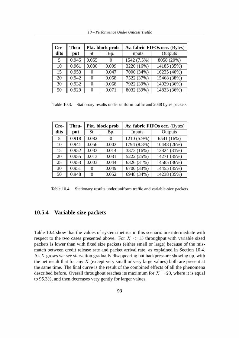
10 – Performance Under Unicast Traffic
Cre- Thru- Pkt. block prob. Av. fabric FIFOs occ. (Bytes)dits put St. Bp. Inputs Outputs
5 0.945 0.055 0 1542 (7.5%) 8058 (20%)10 0.961 0.030 0.009 3220 (16%) 14185 (35%)15 0.953 0 0.047 7000 (34%) 16235 (40%)20 0.942 0 0.058 7522 (37%) 15468 (38%)30 0.932 0 0.068 7922 (39%) 14929 (36%)50 0.929 0 0.071 8032 (39%) 14833 (36%)
Table 10.3. Stationary results under uniform traffic and 2048 bytes packets
Cre- Thru- Pkt. block prob. Av. fabric FIFOs occ. (Bytes)dits put St. Bp. Inputs Outputs
5 0.918 0.082 0 1210 (5.9%) 6541 (16%)10 0.941 0.056 0.003 1794 (8.8%) 10448 (26%)15 0.952 0.033 0.014 3373 (16%) 12824 (31%)20 0.955 0.013 0.031 5222 (25%) 14271 (35%)25 0.953 0.003 0.044 6326 (31%) 14585 (36%)30 0.951 0 0.049 6700 (33%) 14455 (35%)50 0.948 0 0.052 6948 (34%) 14238 (35%)
Table 10.4. Stationary results under uniform traffic and variable-size packets
10.5.4 Variable-size packets
Table 10.4 show that the values of system metrics in this scenario are intermediate withrespect to the two cases presented above. ForX < 15 throughput with variable sizedpackets is lower than with fixed size packets (either small orlarge) because of the mis-match between credit release rate and packet arrival rate, as explained in Section 10.4.As X grows we see starvation gradually disappearing but backpressure showing up, withthe net result that for anyX (except very small or very large values) both are present atthe same time. The final curve is the result of the combined effects of all the phenomenadescribed before. Overall throughout reaches its maximum for X = 20, where it is equalto 95.3%, and then decreases very gently for larger values.
93

10 – Performance Under Unicast Traffic
0.9
0.91
0.92
0.93
0.94
0.95
0.96
0.97
0.98
0.99
1
10 20 30 40 50
Thr
ough
put
Credits per output port (X)
2x fabric internal speedup3x fabric internal speedup
16x fabric internal speedup
Figure 10.4. Throughput with increased fabric speed-up under uniform traffic andvariable-size packets
10.6 Improving system performance
System performance is satisfactory in all the scenarios tested so far, throughput beinggreater than 92% under any packet size distribution forX > 5. Starting from the resultsobtained previously we try to understand on which parameters it is worth acting to furtherimprove performance.
10.6.1 Increased internal speed-up in the switching fabric
We first try to vary crossbar speed-up to understand how much HOL-blocking penalizesperformance. Results are reported in Figure 10.4 and Table 10.5 for variable-size packets.Note that the caseK = 16 corresponds to an output-queued switch, in which HOL-blocking and output contention are completely eliminated.
We see thatK = 3 brings small improvement, whereasK = 16 almost no improve-ment. We can deduce that HOL-blocking in the switching fabric has a very small impacton system performance. The reason is that with very high speed-up and smallX systemperformance is limited by starvation, whereas with largeX fabric output queues fill uprapidly and activate backpressure towards the fabric inputports. If a fabric output port issaturated, it cannot accept any new packet and speed-up becomes useless.
A comparison of Table 10.5 and Table 10.4 confirms that fabricoutput queues oc-cupancy increases, whereas fabric input queues occupancy decreases. This leads to a
94

10 – Performance Under Unicast Traffic
Cre- Thru- Pkt. block prob. Av. fabric FIFOs occ. (Bytes)dits put St. Bp. Inputs Outputs
5 0.919 0.081 0 111.1 (0.5%) 6746 (16%)10 0.942 0.055 0.003 275.0 (1.3%) 10838 (26%)20 0.959 0.013 0.028 1971 (9.6%) 15413 (38%)25 0.960 0.001 0.039 2802 (14%) 16497 (40%)30 0.958 0 0.042 3331 (16%) 16742 (41%)50 0.955 0 0.045 3690 (18%) 16901 (41%)
Table 10.5. Stationary results under uniform traffic and variable-size packets, forK =
16
small reduction of backpressure but leaves blocking probability due to starvation almostunchanged.
10.6.2 Extended memory size in the switching fabric
In this scenario a large amount of memory is placed at the fabric inputs and outputs, toavoid backpressure. The maximum amount of packets destinedto a linecard inside theswitching fabric at any point in time isX ×PLC . In the worst case they are all maximum-size packets and occupyX × PLC × Lmax = X × 16 × 2048 = X × 32768 bytes. Wechoose this value for the fabric output ports and set the sizeof fabric input ports to onehalf of it.
Cre- Thru- Pkt. block prob. Av. fabric FIFOs occ. (Bytes)dits put St. Bp. Inputs Outputs
5 0.918 0.082 0 1211 (1.5%) 6552 (4%)10 0.942 0.058 0 1340 (0.8%) 10726 (3.3%)15 0.955 0.045 0 1401 (0.6%) 14342 (2.9%)20 0.963 0.037 0 1450 (0.4%) 17772 (2.7%)25 0.969 0.031 0 1489 (0.4%) 21294 (2.6%)30 0.973 0.027 0 1506 (0.3%) 24255 (2.5%)50 0.983 0.017 0 1561 (0.2%) 36866 (2.3%)
Table 10.6. Stationary results with extended memory under uniform traffic and variable-size packets
Figure 10.5 shows the throughput achieved with the originalmemory size and with
95

10 – Performance Under Unicast Traffic
0.9
0.91
0.92
0.93
0.94
0.95
0.96
0.97
0.98
0.99
1
10 20 30 40 50
Thr
ough
put
Credits per output port (X)
Original mem size (64-2048 bytes packets)Ext mem size (64-2048 bytes packets)
Original mem size (2048 bytes packets)Ext mem size (2048 bytes packets)
Figure 10.5. Throughput with original and extended memory in the fabric
the extended memory size, in the case of variable- and maximum-size packets. With ex-tended memory, throughput grows fairly rapidly as more credits are available, and finallyapproaches 100%. Table 10.6 shows that backpressure is never active, but a small (anddecreasing) amount of starvation is still experienced by packets even for very largeX.This is due to the fact that with so much memory in the switching fabric, the control-loopdelay becomes larger and larger asX increases. The more credits are available, the slowerthey are returned.
The improvement achieved in this scenario is not negligible, but its cost is too high.Fabric memory is perhaps the most scarce resource in the system and it is not reasonableto assume that it is readily available in large quantities. The results presented in thisscenario are only meant to be taken as a reference.
10.6.3 Link speed-up between the switching fabric and the linecards
We finally explore the effects of speed-up on the uplink and the downlink (internal fabricspeed-up is kept equal to 2). We assume a data rate of 34 Gbps, corresponding to a linkspeed-up of34/32 = 1.06. The possibility to change link speed between the linecardsand the switching fabric is another benefit deriving from theasynchronicity of the design.
Figure 10.6 shows the throughput vs. number of credits curves for variable-size andmaximum-size packets, with and without speed-up. We observe that both curves withspeed-up are monotonically increasing, whereas those without have a maximum and then
96

10 – Performance Under Unicast Traffic
0.9
0.91
0.92
0.93
0.94
0.95
0.96
0.97
0.98
0.99
1
10 20 30 40 50
Thr
ough
put
Credits per output port (X)
Link at 32 Gbps and variable size packetsLink at 34 Gbps and variable size packets
Link at 32 Gbps and 2048 bytes packetsLink at 34 Gbps and 2048 bytes packets
Figure 10.6. Throughput with link speed-up between the switching fabric and thelinecards
start decreasing. Moreover, the asymptotic values obtained for largeX are much better:both with maximum-size and variable-size packets throughput grows beyond 98%.
Cre- Thru- Pkt. block prob. Av. fabric FIFOs occ. (Bytes)dits put St. Bp. Inputs Outputs
5 0.920 0.080 0 1056 (5.1%) 4513 (11%)10 0.944 0.056 0 1191 (5.8%) 6268 (15%)15 0.957 0.043 0 1363 (6.7%) 7286 (18%)20 0.965 0.034 0.001 1607 (7.8%) 7979 (19%)25 0.971 0.027 0.002 1810 (8.8%) 8397 (21%)30 0.975 0.023 0.002 2020 (9.9%) 8868 (22%)50 0.984 0.014 0.002 2342 (11%) 9638 (24%)
Table 10.7. Stationary results under uniform traffic and variable-size packets, in the caseof communication links between the switching fabric and thelinecards equal to 34 Gbps
Table 10.7 reports numerical data for the variable-size packets case. Fabric outputqueues occupancy is low and grows very slowly, as the queues are drained faster. Lowerfabric output queues occupancy also translates to lower fabric input queues occupancy,
97
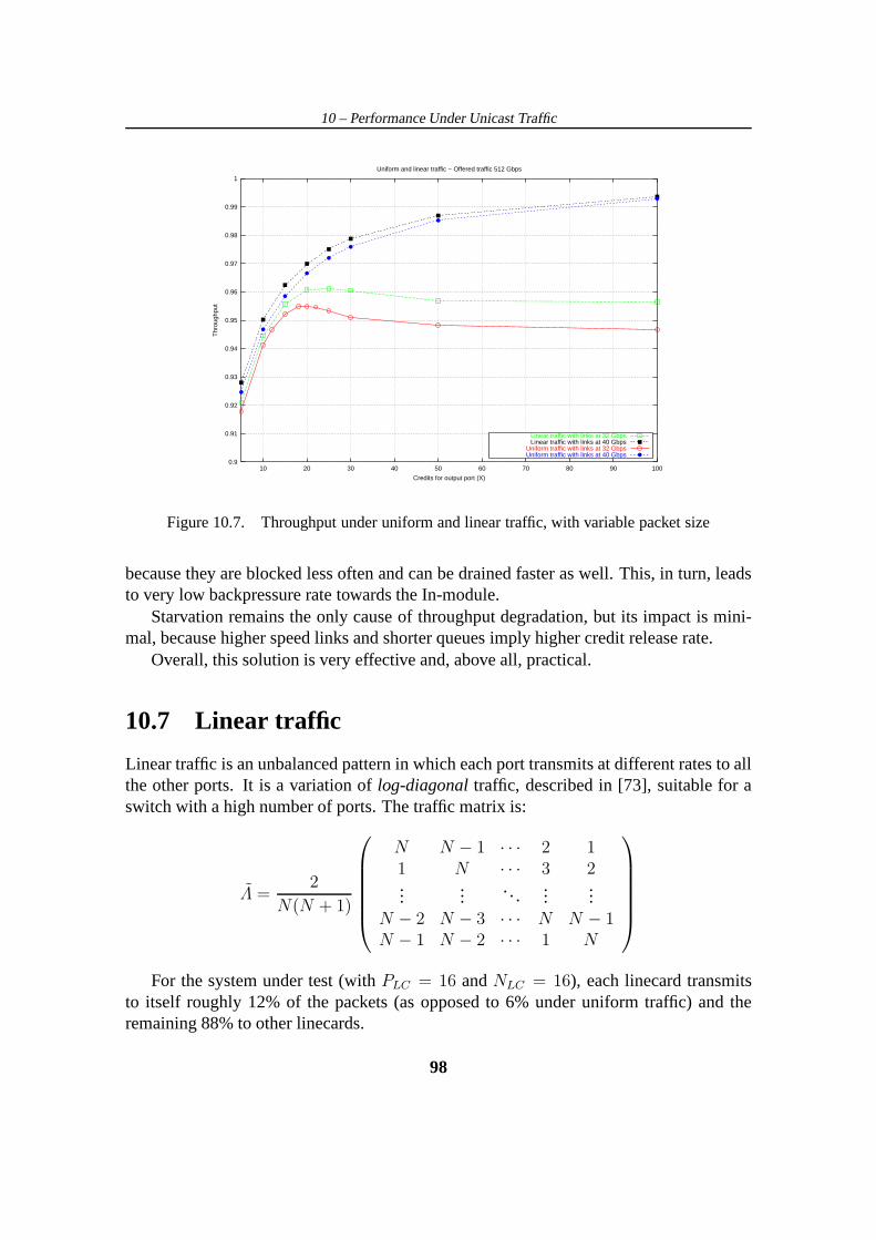
10 – Performance Under Unicast Traffic
0.9
0.91
0.92
0.93
0.94
0.95
0.96
0.97
0.98
0.99
1
10 20 30 40 50 60 70 80 90 100
Thr
ough
put
Credits for output port (X)
Uniform and linear traffic − Offered traffic 512 Gbps
Linear traffic with links at 32 GbpsLinear traffic with links at 40 Gbps
Uniform traffic with links at 32 GbpsUniform traffic with links at 40 Gbps
Figure 10.7. Throughput under uniform and linear traffic, with variable packet size
because they are blocked less often and can be drained fasteras well. This, in turn, leadsto very low backpressure rate towards the In-module.
Starvation remains the only cause of throughput degradation, but its impact is mini-mal, because higher speed links and shorter queues imply higher credit release rate.
Overall, this solution is very effective and, above all, practical.
10.7 Linear traffic
Linear traffic is an unbalanced pattern in which each port transmits at different rates to allthe other ports. It is a variation oflog-diagonaltraffic, described in [73], suitable for aswitch with a high number of ports. The traffic matrix is:
Λ =2
N(N + 1)
N N − 1 · · · 2 11 N · · · 3 2...
.... . .
......
N − 2 N − 3 · · · N N − 1N − 1 N − 2 · · · 1 N
For the system under test (withPLC = 16 andNLC = 16), each linecard transmitsto itself roughly 12% of the packets (as opposed to 6% under uniform traffic) and theremaining 88% to other linecards.
98

10 – Performance Under Unicast Traffic
Figure 10.7 compares the performance obtained under uniform and linear traffic, forvariable link speed-up (32 Gbps or 40 Gbps). Performance under linear traffic is slightlybetter than under uniform traffic, proving the fact that the fabric does not suffer fromtraffic unbalance, but actually benefits from reduced contention.
As in the uniform traffic scenario, performance is significantly improved with moder-ate speed-up on the uplinks and downlinks.
99

Chapter 11
Performance Under Multicast Traffic
Delivery requirements for multicast traffic are more variedthan for unicast and stronglydepend on the application. For example, data replication among multiple sites may requireabsolute delivery guarantee, whereas other applications such as video broadcasting mightallow, and in case of congestion even encourage, packets discard. Fibre Channel standardsprovide two classes of service for multicast [74]. The first is datagram-like and potentiallyunreliable, because end-nodes do not explicitly acknowledge received packets and donot perform end-to-end flow control. The other, instead, is connection-oriented, requiresend-nodes to acknowledge received packets and perform end-to-end flow control.
We study system performance under multicast traffic when twodifferent flow-controlpolicies are employed:
1. The system does not try to regulate incoming traffic in any way. All backpressuremechanisms are disabled and whenever a packet cannot be stored in a buffer, it issimply discarded.
2. The system employs backpressure between buffering stages to prevent overflows,as described in Chapter 9. Backpressure signals are not selective and block all flowstraversing the buffer. Packets in principle could be discarded by the fabric if theyremain blocked for too long1 (Section 9.4.2).
11.1 Simulation Model
For the analysis of system performance under multicast traffic we adopt a more abstractmodel of linecard buffers with respect to the description ofSection 9.4.1 . [75]. In partic-ular, we neglect the presence of two stages of queues on the ingress side and consider asingle module that jointly represents the PSM and the In-module. This component, which
1Actually, with current system settings and under the hypothesis that output ports drain data at line-rate,calculations show that timeoutTo cannot expire, so packets are never discarded by the fabric.
100

11 – Performance Under Multicast Traffic
Outp. PLC
Outp. 1Outp. 2Inp. 2Inp. 1 Inp. PLC
In−module Out−module
Figure 11.1. Linecard simulation model for multicast
we still call “In-module”, consists of a single large bufferorganized as a FIFO queue, di-vided in slots of size equal to a MTU. Total capacity is statically partitioned among inputports; ports can enqueue new packets only if space is available in their memory share.The Out-module is also organized as a single FIFO queue, as previously mentioned. Thelinecard model implemented in the simulator is show in Figure 11.1.
The Out-module and the switching fabric are modeled according to the description ofChapter 9.
11.2 Simulation settings
The simulated system is a16 × 16 switch with 4 linecards hosting 4 input/output portseach. Each port runs at 10 Gbps, hence the aggregate bandwidth is 160 Gbps. Table 11.1summarizes the values of system parameters we have used.
11.3 Traffic model
In all experiments, three packet size distributions have been considered:
• minimum size (80 bytes) only,
• maximum size (2000 bytes) only,
• uniform between 80 and 2000 bytes, with 40 bytes increment.
101

11 – Performance Under Multicast Traffic
Parameter Symbol Value
Input - Output portsInput-Output ports per linecard PLC 4Linecards in the system NLC 4Overall number of Input-Output ports N 16
Link speeds for data and signalingInput - Output ports (data path) — 10 GbpsLinecard↔ crossbar (data path) — 40 Gbps
Packet sizeMinimum packet dimension — 80 bytesMaximum packet dimension MTU 2000 bytes
In-module & Out-module BuffersIn-module shared buffer size — 8000 MTUs = 16 MBOut-module shared buffer size — 320 KB
Switching FabricInternal speed-up K 3Input fabric buffer size — 10 KBOutput fabric buffer size — 20 KBSecond timeout value To 15µs
Table 11.1. Summary of the main architecture parameters
Each active source emits a packet with probabilityρin, 0 ≤ ρin ≤ 1 and with probability1 − ρin remains idle for a period with the same distribution of the packet duration, whichcan be fixed (minimum or maximum size packets only) or variable (packet size uniformlydistributed).
If the backpressure signal from the In-module is active, generation of new packets isblocked. As soon as the backpressure signal is deactivated,the source can start generatingagain. The effective average input load generated by a source is ρin ≤ ρin.
Packets generated while a source is experiencing backpressure are simply discarded.We have decided to neglect the fact that in reality these packets would accumulate at thesource (Section 8.3.2) because it would introduce a perturbation of the input load andcomplicate throughput analysis, especially in overload conditions.
The average offered load to an output port isρout and it is equal to the sum of theρin
of input ports transmitting to that output times the probability of selecting that output. Ifρout > 1, traffic is not admissible and the output port is overloaded.
102

11 – Performance Under Multicast Traffic
0 0
1
2
3 3
2
1
Line CardIn−Module
Line CardOut−Module
(0,0)(0,1)(0,2)(0,3)
(1,0)(1,1)(1,2)(1,3)
(2,0)(2,1)(2,2)(2,3)
(3,0)(3,1)(3,2)(3,3)
(0,0)(0,1)(0,2)(0,3)
(1,0)(1,1)(1,2)(1,3)
(2,0)(2,1)(2,2)(2,3)
(3,0)(3,1)(3,2)(3,3)
0123
4567
89
1011
12131415
0123
4567
89
1011
12131415
Inputs −→ Outputs(0,0) −→ [(0,0) - (1,0) - (2,0) - (3,0)](1,1) −→ [(0,1) - (1,1) - (2,1) - (3,1)](2,2) −→ [(0,2) - (1,2) - (2,2) - (3,2)](3,3) −→ [(0,3) - (1,3) - (2,3) - (3,3)]
Figure 11.2. Broadcast traffic scenario with one active porton each linecard
As discussed in Section 9.4, the replication of a multicast packet to multiple ports onthe same linecard is instantaneous and does not have any impact on the switching of pack-ets between linecards. Thus, in all the traffic patterns we have selected, the destinationports in the fanout set always reside on different linecards. If the fanout of a packet isF ,then it must be replicated toF linecards.
11.4 Broadcast traffic scenario - One active port per linecard
We first present results obtained in two different broadcastscenarios. We call “broadcast”any scenario in which everylinecard transmits packets to alllinecards in the system,regardless of how many input ports are active and how many output ports they transmitto.
In Figure 11.2 the multicast pattern under consideration isshown. Each port is iden-tified by the pair (x,y), wherex is the linecard number andy the port number on thelinecard. On each linecard, only one input port is active andit transmits packets to fouroutput ports on four different linecards. Each output port receives packets from a single
103

11 – Performance Under Multicast Traffic
0.10
0.20
0.30
0.40
0.50
0.60
0.70
0.80
0.90
1.00
0.10 0.20 0.30 0.40 0.50 0.60 0.70 0.80 0.90 1.00
Thr
ough
put
Input Load = Output Load
BACKPRESSURE ON
80 bytes packets2000 bytes packets
80-2000 bytes packets0.10
0.20
0.30
0.40
0.50
0.60
0.70
0.80
0.90
1.00
0.10 0.20 0.30 0.40 0.50 0.60 0.70 0.80 0.90 1.00
Thr
ough
put
Input Load = Output Load
BACKPRESSURE OFF
80 bytes packets2000 bytes packets
80-2000 bytes packets
Figure 11.3. Throughput vs. offered load (broadcast scenario, one active port on eachlinecard)
input port. It follows that traffic is always admissible for any input load0 ≤ ρin ≤ 1 andthatρout = ρin.
Figure 11.3 shows average throughput as a function of the total load offered to a singleoutput port, when backpressure mechanisms are enabled (ON)or disabled (OFF).
Despite the high number of conflicts in the crossbar, in both cases the switch sustainsthe traffic pattern and throughput closely matches the offered load. This is due to the factthat only one port is active on each linecard: the active input port generates as a maximum10 Gbps of data, which is equivalent to 40 Gbps at the fabric output port due to the fanout4. Hence the fabric is always loaded at100% of its capacity.
Table 11.2 reports the numerical values of the average fabric queues occupation atdifferent traffic load. As expected, fabric input and outputqueue occupancy is quite low.When backpressure is enabled, input queue occupancy is slightly higher, meaning thatoutput queues occasionally reach full occupancy and block input queues. Notice that thetable refers to the case of maximum size packets only, when the fabric queues can host asmall number of packets.
11.5 Broadcast scenario - Four active ports on each linecard
In this scenario all input ports are active and transmit packets to four output ports onfour different linecards. The pattern is described in the following table, using the samenumbering scheme of Figure 11.2.
104

11 – Performance Under Multicast Traffic
Backpressure ON Backpressure OFF
OutputLoad0.800.901.00
Through- Xbar Queueput In’s Out’s0.80 5.8 % 13.2 %0.90 7.0 % 15.7 %1.00 8.2 % 21.6 %
Through- Xbar Queueput In’s Out’s0.80 1.4 % 17.7 %0.90 1.6 % 21.3 %1.00 1.8 % 25.1 %
Table 11.2. Average occupation of fabric input-output memories (broadcast scenario,one active port per linecard, 2000 bytes packets)
Inputs −→ Outputs(0,0) + (1,0) + (2,0) + (3,0) −→ [(0,0) - (1,0) - (2,0) - (3,0)](0,1) + (1,1) + (2,1) + (3,1) −→ [(0,1) - (1,1) - (2,1) - (3,1)](0,2) + (1,2) + (2,2) + (3,2) −→ [(0,2) - (1,2) - (2,2) - (3,2)](0,3) + (1,3) + (2,3) + (3,3) −→ [(0,3) - (1,3) - (2,3) - (3,3)]
As each output port receives packets from4 input ports,ρout = 4 × ρin and traffic isadmissible ifρin ≤ 0.25. By settingρin > 0.25 we can generate non-admissible trafficload and observe how the system behaves in overloading conditions.
Notice that from the fabric point of view this scenario is similar to the previous one:all packets coming from a linecard are directed to all linecards and the average load onthe fabric input links is 10 Gbps forρin = 0.25. An important difference regards theburstiness of the traffic arriving on the fabric input links.In this scenario multiple inputports on a linecard can transmit at the same time, effectively generating up to 40 Gbps oftraffic towards the fabric, whereas in the previous scenariothe load was always strictlylimited to 10 Gbps.
Throughput vs. offered output load curves are shown in Figure 11.4. On the top of thegraphs the corresponding input load is also indicated.
When backpressure is enabled, throughput closely matches the offered load and satu-rates to100% for ρin = 0.25. When backpressure is not used, on the contrary, the systemstarts experiencing losses when the offered load grows beyond 90%. This is due to thefact that the increased burstiness of the traffic entering the fabric can cause the fabric out-put queues to temporarily saturate even in underload conditions. Packets that reach a fullfabric output queue are simply discarded and throughput decreases. In overload condi-tions throughput slowly grows to100%, as packets in excess compensate for those that arediscarded. Note that the phenomenon is more evident for maximum-size packets, whenthe queues can host fewer packets, but it is present also whenpacket size is variable.
This analysis is confirmed by the numerical results reportedin Tables 11.3 and 11.4,referring to the case of maximum size packets. Table 11.3 shows that, when backpressure
105

11 – Performance Under Multicast Traffic
0.80
0.85
0.90
0.95
1.00
0.80 0.85 0.90 0.95 1.00 1.05 1.10 1.15 1.20 1.25 1.30
0.200 0.225 0.250 0.275 0.300 0.325
Thr
ough
put
Output Load
BACKPRESSURE ON
Input Load
80 bytes packets2000 bytes packets
80-2000 bytes packets0.80
0.85
0.90
0.95
1.00
0.80 0.85 0.90 0.95 1.00 1.05 1.10 1.15 1.20 1.25 1.30
0.200 0.225 0.250 0.275 0.300 0.325
Thr
ough
put
Output Load
BACKPRESSURE OFF
Input Load
80 bytes packets2000 bytes packets
80-2000 bytes packets
Figure 11.4. Throughput vs. offered load (broadcast scenario, four active ports on eachlinecard)
Output Throughput Throughput LossLoad In-Mod Xbar In Xbar Out Out-Mod0.80 0.800 (100 %) 0 % 0 % 0 % 0 %0.90 0.893 (99.2 %) 0 % 0 % 0.8 % 0 %0.94 0.923 (98.2 %) 0 % 0 % 1.8 % 0 %0.98 0.949 (96.8 %) 0 % 0 % 3.2 % 0 %1.00 0.960 (96.0 %) 0 % 0 % 4.0 % 0 %
1.10 0.992 (90.2 %) 0 % 0 % 9.8 % 0 %1.20 1.000 (83.3 %) 0 % 0 % 16.7 % 0 %
Table 11.3. Throughput loss (broadcast scenario, four active ports on each linecard,backpressure OFF, 2000 bytes packets)
is off, packets are discarded only at fabric output queues. Table 11.4 reports averagefabric queues occupancy. Fabric output queues fill up rapidly when the offered outputload becomes larger than0.90. If backpressure is on, input queues occupancy grows aswell, whereas if it is off, this occupancy remains low.
11.6 “Residue” traffic pattern
We now consider traffic patterns that are known to be particularly critical for input-queuedswitches [30]. These patterns are composed by packets that have a small fanout yet gen-erate a high number of output contentions. It is thus possible to impose high packets
106

11 – Performance Under Multicast Traffic
Backpressure ON Backpressure OFF
OutputLoad0.900.940.981.00
1.101.20
Through- Xbar Queueput In’s Out’s0.90 5.6 % 35.2 %0.94 9.9 % 48.4 %0.98 29.7 % 71.3 %1.00 93.3 % 92.2 %
1.00 94.6 % 91.4 %1.00 94.6 % 92.2 %
Through- Xbar Queueput In’s Out’s0.89 3.9 % 31.1 %0.92 4.2 % 38.2 %0.95 4.5 % 46.5 %0.96 4.7 % 51.7 %
0.97 4.8 % 55.3 %1.00 5.0 % 60.2 %
Table 11.4. Average fabric queue occupancy (broadcast scenario, four active ports oneach linecard, 2000 bytes packets)
injection rate without violating the admissibility condition (thanks to the small fanout)and, at the same time, stress the switching fabric (due to thehigh number of contentions).As fabric speed-up may not be sufficient to accommodate all contending packets, someof them receives partial service, i.e. aresidueis left at the fabric input queue. For thisreason, we name this kind of traffic patterns “Residue”.
11.6.1 “Residue 2” traffic pattern
0,12,30,12,3
0,21,30,21,3
Linecard 1
Linecard 0
0,12,30,12,3
0,21,30,21,3
Linecard 3
Linecard 2
Figure 11.5. “Residue” multicast traffic pattern with fanout 2, from the fabric point ofview
The first pattern we consider is summarized in the following table:
107

11 – Performance Under Multicast Traffic
0.80
0.85
0.90
0.95
1.00
0.80 0.85 0.90 0.95 1.00 1.05 1.10 1.15 1.20 1.25 1.30
0.40 0.45 0.50 0.55 0.60 0.65
Thr
ough
put
Output Load
BACKPRESSURE ON
Input Load
80 bytes packets2000 bytes packets
80-2000 bytes packets0.80
0.85
0.90
0.95
1.00
0.80 0.85 0.90 0.95 1.00 1.05 1.10 1.15 1.20 1.25 1.30
0.40 0.45 0.50 0.55 0.60 0.65
Thr
ough
put
Output Load
BACKPRESSURE OFF
Input Load
80 bytes packets2000 bytes packets
80-2000 bytes packets
Figure 11.6. Throughout vs. offered load (Residue pattern,fanout 2)
Inputs −→ Outputs Inputs −→ Outputs(0,0) −→ [(0, 0) - (1, 0)] (0,2) −→ [(0, 2) - (1, 2)](0,1) −→ [(2, 1) - (3, 1)] (0,3) −→ [(2, 3) - (3, 3)](1,0) −→ [(0, 0) - (2, 0)] (1,2) −→ [(0, 2) - (2, 2)](1,1) −→ [(1, 1) - (3, 1)] (1,3) −→ [(1, 3) - (3, 3)](2,0) −→ [(0, 0) - (1, 0)] (2,2) −→ [(0, 2) - (1, 2)](2,1) −→ [(2, 1) - (3, 1)] (2,3) −→ [(2, 3) - (3, 3)](3,0) −→ [(0, 0) - (2, 0)] (3,2) −→ [(0, 2) - (2, 2)](3,1) −→ [(1, 1) - (3, 1)] (3,3) −→ [(1, 3) - (3, 3)]
The same pattern, seen from the fabric point of view, is depicted in Figure 11.5. Packetscoming from a linecard always contend with at least two packets from other linecards.For instance, packets coming fromLC 0 always have one conflict with packets comingfrom LC 1 andLC 3 and one conflict on average with packets coming fromLC 2.
Each linecard has four active input ports and each output port is loaded by two inputs,so traffic is admissible ifρin ≤ 0.5.
Figure 11.6 shows throughput vs. offered load curves when backpressure mechanismsare set ON or OFF.
When backpressure mechanisms are OFF, system performance is similar to that ob-tained in the previous scenario, both in underload and in overload conditions. When back-pressure mechanisms are ON, on the contrary, significant differences can be observed.System throughput is close to ideal when the offered load is less than∼ 0.96, but at thatpoint it stops growing and actually starts decreasing. The trend can be better observed inFigure 11.7 where offered load is varied up to its maximum value (ρin = 1.0, ρout = 2.0).Throughput loss is especially evident when maximum size packets are used but, is signif-icant also when packet size is uniformly distributed. With minimum size packets, on the
108

11 – Performance Under Multicast Traffic
0.800.820.840.860.880.900.920.940.960.981.00
0.8 0.9 1.0 1.1 1.2 1.3 1.4 1.5 1.6 1.7 1.8 1.9 2.0
0.4 0.5 0.6 0.7 0.8 0.9 1.0
Thr
ough
put
Output Load
Input Load
80 bytes packets2000 bytes packets
80-2000 bytes packets
Figure 11.7. Throughout vs. offered load (Residue pattern,fanout 2, backpressure ON)
Input Output Throughput Average Xbar QueueLoad Load service In’s Out’s0.40 0.80 0.800 1.471 4.3 % 16.9 %0.45 0.90 0.899 1.374 7.1 % 29.6 %0.47 0.94 0.940 1.266 17.4 % 42.8 %0.49 0.98 0.973 1.041 86.6 % 64.9 %0.50 1.00 0.973 1.040 86.6 % 64.9 %
0.55 1.10 0.950 1.059 86.9 % 60.8 %0.60 1.20 0.916 1.067 87.3 % 56.0 %
Table 11.5. Performance results with “Residue” pattern (fanout 2, backpressure ON,2000 bytes packets)
contrary, no loss is experienced.Table 11.5 reports fabric queues occupancy when maximum size packets are used. We
can see that input queues occupancy grows rapidly asρout approaches0.96 and saturatesto ∼ 87%. Output queues occupancy, on the contrary, reaches its maximum at0.96 andsteadily decreases afterward.
To understand this behavior, we must focus on what happens atthe In-modules. Ifthe average fabric input queues occupancy is high, In-modules are subject to backpres-sure very often, and they fill up as well. When the In-module memory is almost full,backpressure towards the sources is activated. As the In-module memory is staticallypartitioned, each source enters and exits backpressure individually; in particular, sourcesthat recently have generated more aggressively enter backpressure earlier. When a source
109

11 – Performance Under Multicast Traffic
9.95e+06 9.96e+06 9.97e+06 9.98e+06 9.99e+06 1e+07
Pac
ket t
ype
Time (slot)
ρin = 0.45 - ρout = 0.90
(0,1)
(2,3)
9.95e+06 9.96e+06 9.97e+06 9.98e+06 9.99e+06 1e+07
Pac
ket t
ype
Time (slot)
ρin = 0.80 - ρout = 1.60
(0,1)
(2,3)
(a) (b)
Figure 11.8. Time traces of packets entering the fabric input 0, at low load (a) and highload (b)
experiences backpressure, the process of packets enteringthe linecard changes. Consider,for instance,LC 0: port (0,0) and (0,2) generate only packets destined to linecards{0,1},whereas ports (0,1) and (0,3) generate only packets destined to linecards{2,3}. If allports on the linecard are active, on average half of the enqueued packets are destined tolinecards{0,1} and the other half to linecards{2,3}. Besides, they are roughly alternated,because all sources generate uncorrelated packets. On the contrary, if a{0,1} source isblocked, more packets destined to linecards{2,3} are enqueued than packets aimed atlinecards{0,1}. It can even happen that both of{0,1} sources are backpressured at thesame time and a long burst of{2,3} packets enter the In-module. This long burst willreach the fabric input queues as well.
Figure 11.8 shows a trace of packets entering the fabric input 0 queue at low (a) andhigh (b) load over50000, hence0.4 ms. timeslots. The high load graph displays∼ 330packets, and the bursts are approximately30 packets long. Burstiness naturally leadsto performance penalties. Conflicting bursts in the fabric input queues prevent efficientusage of the crossbar switching capacity. Some linecard maynot receive packets for longperiods, despite the fact that many packets destined to themare present in the queue. Thisis a form of head-of-the-line blocking due to the usage of a single queue for multicasttraffic.
Notice that this phenomenon is self-sustaining: a source that enters backpressure re-mains blocked for a long time if large bursts of packets from different sources are presentahead in the In-module queue. The hysteresis mechanism usedto activate and deactivate
110

11 – Performance Under Multicast Traffic
backpressure towards sources further facilitates this phenomenon: a blocked port can-not transmit until a minimum number of packets belonging to it are removed from theIn-module queue.
When small packets are used, the In-module queue is drained much fasterin terms ofnumber of packets per unit of time, so sources remain blocked for shorter periods of timeand long bursts do not form.
Finally, asρin approaches1, sources tend to synchronize (because they all generateequal size packets almost back-to-back), so they enter and exit backpressure at the sametime and burst length decreases. A corresponding throughput increase is visible in Fig-ure 11.7 forρout ≥ 1.7. If variable size packets are used, sources do not synchronize andno throughput improvement is observed.
11.6.2 Modified “residue” traffic pattern with fanout 2
To evaluate system performance under the Residue traffic pattern but without the inducedburstiness, we allow all sources on a linecard to generate with equal probability bothkind of packets. For example, all sources transmitting fromLC 0 generate with equalprobability packets destined to linecards{0,1} and packets destined to linecards{2,3}.With this “modified” pattern (represented in the table below) we make sure that bursts donot form regardless of how many sources are experiencing backpressure at any time.
Inputs −→ Outputs Inputs −→ Outputs(0,0) −→ [(0, 0) - (1, 0)] - [(2, 0) - (3, 0)] (0,2) −→ [(0, 2) - (1, 2)] - [(2, 2) - (3, 2)](0,1) −→ [(0, 1) - (1, 1)] - [(2, 1) - (3, 1)] (0,3) −→ [(0, 3) - (1, 3)] - [(2, 3) - (3, 3)](1,0) −→ [(0, 0) - (2, 0)] - [(1, 0) - (3, 0)] (1,2) −→ [(0, 2) - (2, 2)] - [(1, 2) - (3, 2)](1,1) −→ [(0, 1) - (2, 1)] - [(1, 1) - (3, 1)] (1,3) −→ [(0, 3) - (2, 3)] - [(1, 3) - (3, 3)](2,0) −→ [(0, 0) - (1, 0)] - [(2, 0) - (3, 0)] (2,2) −→ [(0, 2) - (1, 2)] - [(2, 2) - (3, 2)](2,1) −→ [(0, 1) - (1, 1)] - [(2, 1) - (3, 1)] (2,3) −→ [(0, 3) - (1, 3)] - [(2, 3) - (3, 3)](3,0) −→ [(0, 0) - (2, 0)] - [(1, 0) - (3, 0)] (3,2) −→ [(0, 2) - (2, 2)] - [(1, 2) - (3, 2)](3,1) −→ [(0, 1) - (2, 1)] - [(1, 1) - (3, 1)] (3,3) −→ [(0, 3) - (2, 3)] - [(1, 3) - (3, 3)]
Throughput vs. offered load curves for this scenario are shown in Figure 11.9 and somenumerical values are reported in Table 11.6. We clearly see that throughput still reachesits maximum value forρout ≃ 0.96, but does not decrease afterward. Correspondingly,fabric output queues occupancy grows up to63% and remains at that level forρout > 0.96.Switch performance is satisfactory: despite the hardness of the traffic pattern, maximumthroughput loss is5% for 2000 bytes packets and4% for variable size packets.
111

11 – Performance Under Multicast Traffic
0.80
0.85
0.90
0.95
1.00
0.8 0.9 1.0 1.1 1.2 1.3 1.4 1.5 1.6 1.7 1.8 1.9 2.0
0.4 0.5 0.6 0.7 0.8 0.9 1.0
Thr
ough
put
Output Load
BACKPRESSURE ON
Input Load
80 bytes packets2000 bytes packets
80-2000 bytes packets
Figure 11.9. Throughput vs. offered load (modified Residue pattern, fanout 2)
Input Output Throughput Average Xbar QueueLoad Load service In’s Out’s0.40 0.80 0.800 1.478 4.4 % 19.6 %0.45 0.90 0.902 1.318 13.1 % 37.6 %0.47 0.94 0.941 1.113 47.5 % 55.3 %0.49 0.98 0.953 1.010 86.1 % 63.2 %0.50 1.00 0.953 1.003 86.2 % 63.4 %
0.55 1.10 0.952 1.009 86.2 % 63.2 %0.60 1.20 0.953 1.007 86.1 % 63.5 %
Table 11.6. Stationary results of modified residue pattern (fanout 2) with backpressureON and 2 Kbytes packets
11.6.3 “Residue 3” traffic pattern
In this section we try a Residue traffic pattern with fanout 3,that further stresses theswitching fabric. The pattern is represented from the fabric point of view in Figure 11.10.
Flows have fanout3 and each packet has at least two conflicts with packets comingfrom any other linecard. For instance, packets coming fromLC 0 always have two con-flicts with packets coming fromLC 1 andLC 3, as well as two or three conflicts withpackets coming fromLC 2.
Destination output ports are arranged in such a way that, on average, each output portis loaded by3 input ports. In particular, each input port generates two kind of packets,aimed at thesamethree linecards. Traffic is admissible for0 ≤ ρin ≤ 0.333.
Conditions that led to the generation of long bursts of packets with the same fanout
112

11 – Performance Under Multicast Traffic
0,1,30,1,20,1,3 0,1,2
0,2,31,2,30,2,31,2,3
Linecard 0
Linecard 1
0,1,30,1,20,1,3 0,1,2
0,2,31,2,30,2,31,2,3
Linecard 2
Linecard 3
Figure 11.10. “Residue” multicast traffic pattern with linecard packet fanout 3 (fourinput linecards active)
0.80
0.85
0.90
0.95
1.00
0.8 1.0 1.2 1.4 1.6 1.8 2.0 2.2 2.4 2.6 2.8 3.0
0.27 0.33 0.40 0.47 0.53 0.60 0.67 0.73 0.80 0.87 0.93 1.00
Thr
ough
put
Output Load
BACKPRESSURE ON
Input Load
80 bytes packets2000 bytes packets
80-2000 bytes packets0.80
0.85
0.90
0.95
1.00
0.80 0.85 0.90 0.95 1.00 1.05 1.10 1.15 1.20 1.25 1.30
0.267 0.300 0.333 0.367 0.400 0.433T
hrou
ghpu
t
Output Load
BACKPRESSURE OFF
Input Load
80 bytes packets2000 bytes packets
80-2000 bytes packets
(a) (b)
Figure 11.11. Throughout vs. offered load (Residue pattern, fanout 3)
in Section 11.6.1 apply to this scenario as well. Therefore,we basically observe in Fig-ure 11.11 the same behavior, although throughput loss in overloading region is much lessevident (96% vs. 87% in the worst case).
This is due to the larger fanout of packets in this scenario. When a packet is servedby the fabric, it feeds three output queues. Hence, at most one output queue is damagedby bursts at any time. Curves are intermediate between thoseobtained in the “Residue 2”and in the broadcast scenarios.
Finally, if we modify this traffic pattern to avoid bursts, aswe did in Section 11.6.2,we see that throughput remains constant in the overloading region and is higher than98%for any packet size distribution (Figure 11.12).
113

11 – Performance Under Multicast Traffic
0.80
0.85
0.90
0.95
1.00
0.8 1.0 1.2 1.4 1.6 1.8 2.0 2.2 2.4 2.6 2.8 3.0
0.27 0.33 0.40 0.47 0.53 0.60 0.67 0.73 0.80 0.87 0.93 1.00
Thr
ough
put
Output Load
BACKPRESSURE ON
Input Load
80 bytes packets2000 bytes packets
80-2000 bytes packets
Figure 11.12. Throughput vs. offered load (modified Residuepattern, fanout 3)
11.7 Uniform traffic pattern
In this section we analyze system performance under uniformtraffic, i.e. when the fanoutset of each packet is chosen randomly and independently overthe set of all possiblefanouts. Packets can have small or large fanout and the destination output ports do notdepend on the source port.
For each packet, we consider each possible destination individually and we include orexclude it depending on the toss of a coin (if the resulting fanout is zero, the procedure isrepeated). GivenN possible destinations, the average packet fanout is
F = N2N−1
2N − 1≃
N
2
As noted in Section 11.3 the replication of a packet to multiple ports on the same linecarddoes not affect system performance. Hence, we simplify the pattern by forcing eachpacket to be addressed to at most one port on each linecard.
As in our configurationNLC = 4, every port on a linecard can generate a total of2NLC −1 = 15 packets. Of these,4 have fanout1 (unicast),6 have fanout2, 4 have fanout3 and1 has fanout4 (broadcast). This corresponds to an average fanout of32/15 andtraffic is admissible for0 ≤ ρin ≤ 15/32 = 0.48675.
Figure 11.13 (a) and (b) shows throughput vs. offered load when backpressure mech-anisms are enabled and disabled respectively.
When backpressure mechanisms are OFF, system performance is similar to that ob-tained in previous traffic scenarios. When backpressure is enabled, we see that the systemperformance is not impacted by the variability of packet fanouts. Its behavior is similarto that observed with the modified version of the “Residue” traffic pattern. Throughputtracks offered load up toρout = 0.96 and then saturates to96% for 2 Kbytes packets and
114

11 – Performance Under Multicast Traffic
0.80
0.85
0.90
0.95
1.00
0.80 0.85 0.90 0.95 1.00 1.05 1.10 1.15 1.20 1.25 1.30
0.375 0.422 0.469 0.516 0.562 0.609
Thr
ough
put
Output Load
BACKPRESSURE ON
Input Load
80 bytes packets2000 bytes packets
80-2000 bytes packets0.80
0.85
0.90
0.95
1.00
0.80 0.85 0.90 0.95 1.00 1.05 1.10 1.15 1.20 1.25 1.30
0.375 0.422 0.469 0.516 0.562 0.609
Thr
ough
put
Output Load
BACKPRESSURE OFF
Input Load
80 bytes packets2000 bytes packets
80-2000 bytes packets
(a) (b)
Figure 11.13. System performance under uniform traffic pattern. (a): backpressure ON.(b): backpressure OFF.
97% for variable size packets. No losses are observed in the overloading region, as pack-ets are uncorrelated and bursts cannot form, regardless of which sources are blocked bybackpressure.
115

Chapter 12
Conclusions – Part II
We have presented a switching architecture specifically designed for Fibre Channel SANsand we have studied its performance by means of simulation under various unicast andmulticast traffic patterns.
The system was designed for high-performance and high-scalability. A major rolein achieving these goals is played by the asynchronicity of the design that simplifies theimplementation of system modules and provides other important benefits.
The demanding requirements of storage traffic, first and foremost loss-free operation,are satisfied with a blend of flow-control and buffer management techniques. In particular,backpressure at every buffering stage avoids packet lossesunder any circumstances, buffermanagement policies at the In-modules prevent active portsfrom monopolizing availablespace and fine-grained, credit-based, internal flow-control operated by the central arbiteridentifies and isolates congesting flows.
Simulation results show that performance is very satisfactory under uniform and non-uniform traffic patterns and for different packet-size distributions. Additional experimentsshow that it can be further improved by introducing a small speed-up on the uplinks andthe downlinks.
The switching architecture can be easily extended to support multicast traffic. Thechoice of performing replication in two stages, in the switching fabric and in the Out-modules leads to efficient usage of system resources. The switching fabric operatesaccording to an algorithm that tries to gain the benefits of crossbar replication withoutsacrificing latency.
As the number of potentially active multicast flows grows exponentially with the num-ber of ports, it is not practically feasible to allocate system resources per-flow. In thissystem multicast packets are simply enqueued in FIFO order,both on the ingress and theegress sides of linecards. This certainly leads to HOL blocking and to unfairness, whichbecome especially dangerous if downstream devices are blocking output ports. Interme-diate solutions, entailing a reasonable number of queues and an implementable arbiter arecertainly possible, but haven’t been investigated yet. We should also keep in mind that
116

12 – Conclusions – Part II
strictly lossless behavior for multicast traffic is required only in few particular situationsand that in general discarding packets, though undesirable, is acceptable.
Simulation results show that the system achieves satisfactory performance under var-ious multicast traffic patterns, for various packet-size distributions and both in lossy andloss-free operation. We have identified phenomena that can degrade throughput by in-ducing burstiness on traffic entering the fabric, however, they can only be observed inoverloading conditions and under particularly challenging traffic patterns.
Overall we believe that the results of this study prove that this innovative architectureis particularly fit for director-class data-center switches, thanks to its high-performance,robustness and scalability. The phenomena we have identified and the guidelines we havedevised can be useful to further evolve this architecture orto develop new ones aimed atthe same environment.
117

Bibliography
[1] H. J. Chao, C. Lam, and E. Oki,Broadband Packet Switching Technologies. JohnWiley & sons, Sept. 2001.
[2] A. Pattavina,Switching Theory. John Wiley & sons, 1998.[3] J. Y. Hui,Switching and Traffic Theory for Integrated Broadband Networks. Boston,
MA: Kluwer, 1990.[4] M. Katevenis, G. Passas, D. Simos, I. Papaefstathiou, and N. Chrysos, “Variable
packet size buffered crossbar (cicq) switches,” inProc. IEEE International Confer-ence on Communications (ICC 2004), vol. 2, (Paris, France), pp. 1090–1096, June20–24, 2004.
[5] K. Yoshigoe and K. Christensen, “A parallel-polled virtual output queued switchwith a buffered crossbar,” inProc. IEEE Workshop on High-Performance Switchingand Routing HPSR 2001, (Dallas, TX), pp. 271–275, May 2001.
[6] A. Bianco, P. Giaccone, E. M. Giraudo, F. Neri, and E. Schiattarella, “Perfor-mance analysis of storage area network switches,” inProc. IEEE Workshop onHigh-Performance Switching and Routing HPSR 2005, (Hong Kong), 2005.
[7] W. J. Dally and B. P. Towles,Principles and practices of interconnection networks.San Francisco, CA: Morgan Kaufmann, 2003.
[8] N. Karol, M. Hluchyj, and S. Morgan, “Input versus outputqueueing on a spacedivision switch,”IEEE Trans. Commun., vol. 35, pp. 1347–1356, Dec. 1987.
[9] Y. Tamir and G. Frazier, “High performance multi-queue buffers for vlsi commu-nication switches,” inProc. 15th Ann. Symp. Comp. Archi., pp. 343–354, June1988.
[10] N. McKeown, A. Mekkittikul, V. Anantharam, and J. Walrand, “Achieving 100%throughput in an input-queued switch,”IEEE Trans. Commun., vol. 47, pp. 1260–1267, Aug. 1999.
[11] S. T. Chuang, A. Goel, N. McKeown, and B. Prabhakar, “Matching output queueingwith a combined input output queued switch,”IEEE J. Sel. Areas Commun., vol. 17,pp. 1030–1039, June 1999.
[12] I. Stoica and H. Zhang, “Exact emulation of an output queueing switch by a com-bined input output queueing switch,” inProc. 6th IEEE/IFIP IWQoS ’98, (NapaValley, CA), pp. 218–224, May 1998.
118

Bibliography
[13] J. G. Dai and B. Prabhakar, “The throughput of data switches with and withoutspeed-up,” inProc. IEEE INFOCOM 2000, vol. 2, (Tel Aviv, Israel), pp. 556–564,Mar. 2000.
[14] C. Minkenberg, R. Luijten, F. Abel, W. Denzel, and M. Gusat, “Current issues inpacket switch design,”ACM Computer Commun. Rev., vol. 33, pp. 119–124, Jan.2003.
[15] L. Tassiulas and A. Ephremides, “Stability propertiesof constrained queueing sys-tems and scheduling policies for maximum throughput in multihop radio networks,”IEEE/ACM Trans. Automat. Control, vol. 37, pp. 1936–1948, Dec. 1992.
[16] R. E. Tarjan,Data Structures and Network Algorithms. Murray Hills, NJ: Bell Labs,1983.
[17] T. Anderson, S. Owicki, J. Saxe, and C. Thacker, “High-speed switch scheduling forlocal area networks,”ACM Trans. Comput. Syst, vol. 11, pp. 319–352, Nov. 1993.
[18] N. McKeown, Scheduling Algorithms for Input-Queued Switches. PhD thesis,University of California at Berkeley, 1995.
[19] N. McKeown, “The iSLIP scheduling algorithm for input-queued switches,”IEEE/ACM Trans. Networking, vol. 7, pp. 188–201, Apr. 1999.
[20] H. Chao and J. Park, “Centralized contention resolution schemes for a large-capacityoptical ATM switch,” inProc. IEEE ATM Workshop, (Fairfax, VA), pp. 11–16, May1998.
[21] D. Serpanos and P. Antoniadis, “Firm: A class of distributed scheduling algo-rithms for high-speed ATM switches with multiple input queues,” in Proc. IEEEINFOCOM 2000, vol. 2, (Tel Aviv, Israel), pp. 548–555, Mar. 2000.
[22] Y. Li, S. Panwar, and H. Chao, “On the performance of a dual round-robin switch,” inProc. IEEE INFOCOM 2001, vol. 3, (Anchorage, AK), pp. 1688–1697, Apr. 2001.
[23] A. Mekkittikul and N. McKeown, “A practical schedulingalgorithm to achieve100% thorughput in input-queued switches,” inProc. IEEE INFOCOM ’98, (SanFrancisco, CA), pp. 792–799, Apr. 1998.
[24] M. Ajmone Marsan, A. Bianco, and E. Leonardi, “RPA: A simple, efficient, andflexible policy for input buffered ATM switches,”IEEE Commun. Lett., vol. 1,pp. 83–86, May 1997.
[25] A. Smiljanic, R. Fan, and G. Ramamurthy, “RRGS-round-robin greedy schedulingfor electronic/optical terabit switches,” inProc. IEEE GLOBECOM 1999, (Rio deJaneiro, Brazil), pp. 584–555, Dec. 1999.
[26] Y. Tamir and H.-C. Chi, “Symmetric crossbar arbiters for VLSI communicationswitches,” IEEE Trans. Parallel and Distributed Systems, vol. 4, pp. 13–27, Jan.1993.
[27] W. T. Chen, C. F. Huang, C. Y. L., and W. Y. Hwang, “An efficient cell-scheduling al-gorithm for multicast atm switching systems,”IEEE/ACM Trans. Networking, vol. 8,pp. 517–525, Aug. 2000.
119

Bibliography
[28] P. Gupta and N. McKeown, “Designing and implementing a fast crossbar scheduler,”IEEE Micro, vol. 19, pp. 20–28, Jan./Feb. 1999.
[29] A. Bianco, P. Giaccone, E. Leonardi, F. Neri, and C. Pilgione, “On the number ofinput queues required to support multicast traffic in input queued switches,” inProc.IEEE Workshop on High-Performance Switching and Routing HPSR 2003, (Torino,Italy), pp. 49–54, June 24–27, 2003.
[30] M. Ajmone Marsan, A. Bianco, P. Giaccone, E. Leonardi, and F. Neri, “Multicasttraffic in input-queued switches: Optimal scheduling and maximum throughput,”IEEE/ACM Trans. Networking, vol. 11, pp. 465–477, June 2003.
[31] J. Hayes, R. Breault, and M. Mehmet-Ali, “Performance analysis of a multicastswitch,” IEEE/ACM Trans. Commun., vol. 39, pp. 581–587, Apr. 1991.
[32] J. Y. Hui and T. Renner, “Queueing analysis for multicast packet switching,”IEEETrans. Commun., vol. 42, pp. 723–731, feb/mar/apr 1994.
[33] Z. Liu and R. Righter, “Scheduling multicast input-queued switches,”J. Scheduling,vol. 2, pp. 99–114, 1999.
[34] B. Prabhakar, N. McKeown, and R. Ahuja, “Multicast scheduling for input-queuedswitches,”IEEE J. Sel. Areas Commun., vol. 15, pp. 855–866, June 1997.
[35] “Getting up to speed: The future of supercomputing,” tech. rep., National ResearchCouncil, 2005.
[36] G. F. Pfister, “An introduction to the InfiniBand architecture,” inHigh PerformanceMass Storage and Parallel I/O: Technologies and Applications (H. Jin, T. Cortes,and R. Buyya, eds.), ch. 42, pp. 617–632, New York, NY: IEEE Computer SocietyPress and Wiley, 2001.
[37] G. F. Pfister,In Search of Clusters. Upper Saddle River, NJ: Prentice Hall, 2 ed.,1998.
[38] J. Hennessy and D. Patterson,Computer Architecture - A Quantitative Approach.Morgan Kaufmann Publishers, Elsevier, third ed., May 2002.
[39] S. P. Vander Wiel and D. Lilja, “When caches aren’t enough: data prefetchingtechniques,”IEEE Computer, vol. 30, pp. 23–30, July 1997.
[40] J. Duato, S. Yalamanchili, and L. Ni,Interconnection Networks - An EngineeringApproach. Morgan Kaufmann Publishers, Elsevier, revised ed., 2003.
[41] A. Gara, M. A. Blumrich, D. Chen, G. L.-T. Chiu, P. Coteus, M. E. Giampapa, R. A.Haring, P. Heidelberger, D. Hoenicke, G. V. Kopcsay, T. A. Liebsch, M. Ohmact,S.-B. B. D., T. Takken, and P. Vranas, “Overview of the blue gene/l systemarchitecture,”IBM J. Res. & Dev., vol. 49, pp. 195–212, march/may 2005.
[42] N. R. Adiga, M. A. Blumrich, D. Chen, P. Coteus, A. Gara, M. E. Giampapa,P. Heidelberger, S. Singh, S.-B. B. D., T. Takken, M. Tsao, and P. Vranas, “Bluegene/l torus interconnection network,”IBM J. Res. & Dev., vol. 49, pp. 265–276,march/may 2005.
[43] C. Clos, “A study of non-blocking switching networks,”Bell System TechnicalJournal, vol. 32, pp. 406–424, 1953.
120

Bibliography
[44] A. Jajszczyk, “Nonblocking, repackable, and rearrangeable clos networks: Fiftyyears of the theory evolution,”IEEE Communications Magazine, vol. 41, pp. 28–33,Oct. 2003.
[45] C. W. Wu and T. Feng, “On a class of multistage interconnection networks,”IEEETrans. Computers, vol. 29, pp. 694–702, Aug. 1980.
[46] C. E. Leiserson, “Fat-trees: Universal networks for hardware-efficient supercomput-ing,” IEEE Trans. Computers, vol. 34, pp. 892–201, Oct. 1985.
[47] A. Schacham, B. A. Small, and K. Bergman, “Interconnection networks for high-performance computing – electronics vs. optics,” internalmanuscript, LighwaveResearch Laboratory, Columbia University, Mar. 2004.
[48] G. I. Papadimitriou, C. Papazoglou, and S. A. Pomportis, “Optical switching: Switchfabrics, techniques and architectures,”IEEE J. Lightwave Technol., vol. 21, pp. 384–405, Feb. 2003.
[49] S. Kitamura, K. Komatsu, and M. Kitamura, “Very low power consumption semi-conductor optical amplifier array,”IEEE Photonics Technology Letters, vol. 7,pp. 147–148, Feb. 1995.
[50] F. Masetti, D. Chiaroni, R. Dragnea, R. Robotham, and D.Zriny, “High-speed high-capacity packet-switching fabric: a key system for required flexibility and capacity,”J. Opt. Netw., vol. 2, pp. 255–265, jul 2003.
[51] R. Luijten, C. Minkneberg, R. Hemenway, M. Sauer, and R.Grzybowski, “Vi-able opto-electronic hpc interconnect fabrics,” inProc. ACM Supercomputing 2005,(Seattle, WA, USA), Nov. 2005.
[52] Q. Yang, K. Bergman, G. D. Hughes, and F. Johnson, “Wdm packet routing forhigh-capacity data networks,”IEEE J. Lightwave Technol., vol. 19, pp. 1420–1426,Oct. 2001.
[53] R. Hemenway, R. Grzybowski, C. Minkenberg, and R. Luijten, “Optical-packet-switched interconnect for supercomputer applications,”OSA J. Opt. Netw., vol. 3,pp. 900–913, Dec. 2004.
[54] C. Minkenberg, F. Abel, P. Muller, R. Krishnamurty, M.Gusat, P. Dill, I. Iliadis,R. Luijten, B. Roe Hemenway, R. Grzybowski, and E. Schiattarella, “Designing acrossbar scheduler for hpc applications,”To appear in IEEE Micro, 2006.
[55] C. Minkenberg, F. Abel, P. Muller, R. Krishnamurthy, and M. Gusat, “Control pathimplementation of a low-latency optical HPC switch,” inProc. of Hot Interconnects13, (Stanford, CA), Aug. 17–19 2005.
[56] C. Minkenberg, “Performance of i-SLIP scheduling withlarge round-trip latency,”in Proc. IEEE Workshop on High-Performance Switching and Routing HPSR 2003,(Torino, Italy), pp. 49–54, June 24–27, 2003.
[57] C. Minkenberg, F. Abel, and M. Gusat, “Reliable controlprotocol for crossbararbitration,”IEEE Commun. Lett., vol. 9, pp. 178–180, Feb. 2005.
[58] C. Minkenberg, F. Abel, and E. Schiattarella, “Distributed crossbar schedulers,” in
121

Bibliography
To appear in Proc. IEEE Workshop on High-Performance Switching and Routing(HPSR 2006), (Poland), 2006.
[59] C. Minkenberg, I. Iliadis, and F. Abel, “Low-latency pipelined crossbar arbitration,”in Proc. IEEE GLOBECOM 2004, (Dallas, TX), Dec. 2004.
[60] E. Oki, R. Rojas-Cessa, and H. Chao, “A pipeline-based approach for maximal-sized matching scheduling in input-buffered switches,”IEEE Commun. Lett., vol. 5,pp. 263–265, June 2001.
[61] E. Oki, R. Rojas-Cessa, and H. Chao, “PMM: A pipelined maximal-sized match-ing scheduling approach for input-buffered switches,” inProc. IEEE GLOBECOM2001, vol. 1, (San Antonio, TX), pp. 35–39, Nov. 2001.
[62] E. Schiattarella and C. Minkenberg, “Fair integrated scheduling of unicast and mul-ticast traffic in an input-queued switch,” inTo appead in Proc. IEEE InternationalConference on Communications (ICC 2006), (Istanbul, Turkey), 2006.
[63] “Omnet++ discrete event simulation system.” http://www.omnetpp.org/.[64] K. Pawlikowski, V. Yau, and D. McNickle, “Distributed stochastic discrete-event
simulation in parallel time streams,” inProc. Winter Simulation Conference,pp. 723–730, 1994.
[65] R. Rojas-Cessa, E. Oki, and H. Chao, “CIXOB-k: combinedinput-crosspoint-outputbuffered packet switch,” inProc. IEEE GLOBECOM 2001, vol. 4, (San Antonio,TX), pp. 2654–2660, Nov. 2001.
[66] M. Andrews, S. Khanna, and K. Kumaran, “Integrated scheduling of unicast andmulticast traffic in an input-queued switch,” inProc. IEEE INFOCOM 1999, vol. 3,pp. 1144–1151, Mar. 1999.
[67] M. Song and W. Zhu, “Integrated queueing and schedulingfor unicast and multicasttraffic in input-queued packet switches,” inProc. 2nd IASTED International Confer-ence on Communication and Computer Networks, (M.I.T., Cambridge, MA), Nov.2004.
[68] A. Smiljanic, “Scheduling of multicast traffic in high-capacity packet switches,”IEEE Communications Magazine, pp. 72–77, Nov. 2002.
[69] C. Minkenberg, “Integrating unicast and multicast traffic scheduling in a combinedinput- and output-queued packet-switching system,” inProc. IEEE ICCCN 2000,(Las Vegas, NV), pp. 127–234, Oct. 2000.
[70] N. McKeown and B. Prabhakar, “Scheduling multicast cells in an input-queuedswitch,” in Proc. IEEE INFOCOM 1996, vol. 1, pp. 271–278, Mar. 1996.
[71] T. Clark,Designing Storage Area Networks. Addison Wesley, 2 ed., 2003.[72] J. Satran, K. Meth, C. Sapuntzakis, M. Chadalapaka, andE. Zeidner, “Internet Small
Computer Systems Interface (iSCSI).” RFC 3720 (Proposed Standard), Apr. 2004.[73] P. Giaccone, B. Prabhakar, and D. Shah, “Randomized scheduling algorithms for
high-aggregate bandwidth switches,”IEEE J. Sel. Areas Commun., vol. 21, pp. 546–559, May 2003.
122

Bibliography
[74] ANSI, “Fibre channel - framing and signaling (fc-fs),”INCITS 373-2003, ANSI,Apr. 2003.
[75] A. Bianco, P. Giaccone, E. M. Giraudo, F. Neri, and E. Schiattarella, “Multicastsupport for storage area network switches,” inSubmitted to the IEEE GLOBECOM2006, 2006.
123

124

Table of Acronyms
CIOQ: Combined Input-Output QueuedCOTS: Commercial, Off-the-ShelfCMOS: Complementary Metal-Oxide-SemiconductorCRC: Cyclic Redundant CheckDSM: Distributed Shared-MemoryDWD: Dense Wavelength-Division MultiplexingEDFA: Erbium-Doped Fiber AmplifierE/O: Electro-OpticalFCFS: First Come, First ServedFEC: Forward Error-Correcting CodeFIFO: First In, First OutFPGA Field-Programmable Gate ArrayHOL: Head-Of-the-LineHPC: High-Performance ComputingIP: Internet ProtocolIQ: Input-QueuedLAN: Local Area NetworkMIN: Multistage Interconnection NetworkMPP: Massively Parallel ProcessorMTU: Maximum Tranfer UnitNUMA: Non-Uniform Memory AccessOBS: Optical Burst SwitchingO/E: Opto-ElectricalOSMOSIS: Optical Shared-MemOry Supercomputer Interconnect SystemOQ: Output-QueuedRDQ: Reliable-Delivery QueueRTT: Round-Trip TimeSAN: Storage Area NetworkSMP: Symmetric Multi-ProcessorSOA: Semiconductor Optical AmplifiersTCP: Transport Control ProtocolTTL: Time To LiveUMA: Uniform Memory AccessVOQ: Virtual Output QueueWAN: Wide Area NetworkWDM: Wavelength-Division Multiplexing