
Risk and Financial Management - FANARCO3.4.1 Bernoulli, Buffon, Cramer and Feller 51 3.4.2 Allais...
344
Risk and Financial Management Risk and Financial Management: Mathematical and Computational Methods. C. Tapiero C 2004 John Wiley & Sons, Ltd ISBN: 0-470-84908-8
Transcript of Risk and Financial Management - FANARCO3.4.1 Bernoulli, Buffon, Cramer and Feller 51 3.4.2 Allais...

Risk and Financial Management
Risk and Financial Management: Mathematical and Computational Methods. C. TapieroC© 2004 John Wiley & Sons, Ltd ISBN: 0-470-84908-8

Risk and FinancialManagementMathematical and Computational Methods
CHARLES TAPIEROESSEC Business School, Paris, France

Copyright C© 2004 John Wiley & Sons Ltd, The Atrium, Southern Gate, Chichester,West Sussex PO19 8SQ, England
Telephone (+44) 1243 779777
Email (for orders and customer service enquiries): [email protected] our Home Page on www.wileyeurope.com or www.wiley.com
All Rights Reserved. No part of this publication may be reproduced, stored in a retrieval systemor transmitted in any form or by any means, electronic, mechanical, photocopying, recording,scanning or otherwise, except under the terms of the Copyright, Designs and Patents Act 1988or under the terms of a licence issued by the Copyright Licensing Agency Ltd, 90 TottenhamCourt Road, London W1T 4LP, UK, without the permission in writing of the Publisher.Requests to the Publisher should be addressed to the Permissions Department, John Wiley &Sons Ltd, The Atrium, Southern Gate, Chichester, West Sussex PO19 8SQ, England, or emailedto [email protected], or faxed to (+44) 1243 770571.
This publication is designed to provide accurate and authoritative information in regard tothe subject matter covered. It is sold on the understanding that the Publisher is not engagedin rendering professional services. If professional advice or other expert assistance isrequired, the services of a competent professional should be sought.
Other Wiley Editorial Offices
John Wiley & Sons Inc., 111 River Street, Hoboken, NJ 07030, USA
Jossey-Bass, 989 Market Street, San Francisco, CA 94103-1741, USA
Wiley-VCH Verlag GmbH, Boschstr. 12, D-69469 Weinheim, Germany
John Wiley & Sons Australia Ltd, 33 Park Road, Milton, Queensland 4064, Australia
John Wiley & Sons (Asia) Pte Ltd, 2 Clementi Loop #02-01, Jin Xing Distripark, Singapore 129809
John Wiley & Sons Canada Ltd, 22 Worcester Road, Etobicoke, Ontario, Canada M9W 1L1
Wiley also publishes its books in a variety of electronic formats. Some content that appearsin print may not be available in electronic books.
Library of Congress Cataloging-in-Publication Data
Tapiero, Charles S.Risk and financial management : mathematical and computational methods / Charles Tapiero.
p. cm.Includes bibliographical references.
ISBN 0-470-84908-81. Finance–Mathematical models. 2. Risk management. I. Title.
HG106 .T365 2004658.15′5′015192–dc22 2003025311
British Library Cataloguing in Publication Data
A catalogue record for this book is available from the British Library
ISBN 0-470-84908-8
Typeset in 10/12 pt Times by TechBooks, New Delhi, IndiaPrinted and bound in Great Britain by Biddles Ltd, Guildford, SurreyThis book is printed on acid-free paper responsibly manufactured from sustainable forestryin which at least two trees are planted for each one used for paper production.

This book is dedicated to:
DanielDafnaOrenOscar andBettina

Contents
Preface xiii
Part I: Finance and Risk Management
Chapter 1 Potpourri 031.1 Introduction 031.2 Theoretical finance and decision making 051.3 Insurance and actuarial science 071.4 Uncertainty and risk in finance 10
1.4.1 Foreign exchange risk 101.4.2 Currency risk 121.4.3 Credit risk 121.4.4 Other risks 13
1.5 Financial physics 15Selected introductory reading 16
Chapter 2 Making Economic Decisions under Uncertainty 192.1 Decision makers and rationality 19
2.1.1 The principles of rationality and bounded rationality 202.2 Bayes decision making 22
2.2.1 Risk management 232.3 Decision criteria 26
2.3.1 The expected value (or Bayes) criterion 262.3.2 Principle of (Laplace) insufficient reason 272.3.3 The minimax (maximin) criterion 282.3.4 The maximax (minimin) criterion 282.3.5 The minimax regret or Savage’s regret criterion 28
2.4 Decision tables and scenario analysis 312.4.1 The opportunity loss table 32
2.5 EMV, EOL, EPPI, EVPI 332.5.1 The deterministic analysis 342.5.2 The probabilistic analysis 34
Selected references and readings 38

viii CONTENTS
Chapter 3 Expected Utility 393.1 The concept of utility 39
3.1.1 Lotteries and utility functions 403.2 Utility and risk behaviour 42
3.2.1 Risk aversion 433.2.2 Expected utility bounds 453.2.3 Some utility functions 463.2.4 Risk sharing 47
3.3 Insurance, risk management and expected utility 483.3.1 Insurance and premium payments 48
3.4 Critiques of expected utility theory 513.4.1 Bernoulli, Buffon, Cramer and Feller 513.4.2 Allais Paradox 52
3.5 Expected utility and finance 533.5.1 Traditional valuation 543.5.2 Individual investment and consumption 573.5.3 Investment and the CAPM 593.5.4 Portfolio and utility maximization in practice 613.5.5 Capital markets and the CAPM again 633.5.6 Stochastic discount factor, assets pricing
and the Euler equation 653.6 Information asymmetry 67
3.6.1 ‘The lemon phenomenon’ or adverse selection 683.6.2 ‘The moral hazard problem’ 693.6.3 Examples of moral hazard 703.6.4 Signalling and screening 723.6.5 The principal–agent problem 73
References and further reading 75
Chapter 4 Probability and Finance 794.1 Introduction 794.2 Uncertainty, games of chance and martingales 814.3 Uncertainty, random walks and stochastic processes 84
4.3.1 The random walk 844.3.2 Properties of stochastic processes 91
4.4 Stochastic calculus 924.4.1 Ito’s Lemma 93
4.5 Applications of Ito’s Lemma 944.5.1 Applications 944.5.2 Time discretization of continuous-time
finance models 964.5.3 The Girsanov Theorem and martingales∗ 104
References and further reading 108
Chapter 5 Derivatives Finance 1115.1 Equilibrium valuation and rational expectations 111

CONTENTS ix
5.2 Financial instruments 1135.2.1 Forward and futures contracts 1145.2.2 Options 116
5.3 Hedging and institutions 1195.3.1 Hedging and hedge funds 1205.3.2 Other hedge funds and investment strategies 1235.3.3 Investor protection rules 125
References and additional reading 127
Part II: Mathematical and Computational Finance
Chapter 6 Options and Derivatives Finance Mathematics 1316.1 Introduction to call options valuation 131
6.1.1 Option valuation and rational expectations 1356.1.2 Risk-neutral pricing 1376.1.3 Multiple periods with binomial trees 140
6.2 Forward and futures contracts 1416.3 Risk-neutral probabilities again 145
6.3.1 Rational expectations and optimal forecasts 1466.4 The Black–Scholes options formula 147
6.4.1 Options, their sensitivity and hedging parameters 1516.4.2 Option bounds and put–call parity 1526.4.3 American put options 154
References and additional reading 157
Chapter 7 Options and Practice 1617.1 Introduction 1617.2 Packaged options 1637.3 Compound options and stock options 165
7.3.1 Warrants 1687.3.2 Other options 169
7.4 Options and practice 1717.4.1 Plain vanilla strategies 1727.4.2 Covered call strategies: selling a call and a
share 1767.4.3 Put and protective put strategies: buying a
put and a stock 1777.4.4 Spread strategies 1787.4.5 Straddle and strangle strategies 1797.4.6 Strip and strap strategies 1807.4.7 Butterfly and condor spread strategies 1817.4.8 Dynamic strategies and the Greeks 181
7.5 Stopping time strategies∗ 1847.5.1 Stopping time sell and buy strategies 184
7.6 Specific application areas 195

x CONTENTS
7.7 Option misses 197References and additional reading 204Appendix: First passage time∗ 207
Chapter 8 Fixed Income, Bonds and Interest Rates 2118.1 Bonds and yield curve mathematics 211
8.1.1 The zero-coupon, default-free bond 2138.1.2 Coupon-bearing bonds 2158.1.3 Net present values (NPV) 2178.1.4 Duration and convexity 218
8.2 Bonds and forward rates 2228.3 Default bonds and risky debt 2248.4 Rated bonds and default 230
8.4.1 A Markov chain and rating 2338.4.2 Bond sensitivity to rates – duration 2358.4.3 Pricing rated bonds and the term structure
risk-free rates∗ 2398.4.4 Valuation of default-prone rated bonds∗ 244
8.5 Interest-rate processes, yields and bond valuation∗ 2518.5.1 The Vasicek interest-rate model 2548.5.2 Stochastic volatility interest-rate models 2588.5.3 Term structure and interest rates 259
8.6 Options on bonds∗ 2608.6.1 Convertible bonds 2618.6.2 Caps, floors, collars and range notes 2628.6.3 Swaps 262
References and additional reading 264Mathematical appendix 267
A.1: Term structure and interest rates 267A.2: Options on bonds 268
Chapter 9 Incomplete Markets and Stochastic Volatility 2719.1 Volatility defined 2719.2 Memory and volatility 2739.3 Volatility, equilibrium and incomplete markets 275
9.3.1 Incomplete markets 2769.4 Process variance and volatility 2789.5 Implicit volatility and the volatility smile 2819.6 Stochastic volatility models 282
9.6.1 Stochastic volatility binomial models∗ 2829.6.2 Continuous-time volatility models 00
9.7 Equilibrium, SDF and the Euler equations∗ 2939.8 Selected Topics∗ 295
9.8.1 The Hull and White model and stochasticvolatility 296
9.8.2 Options and jump processes 297

CONTENTS xi
9.9 The range process and volatility 299References and additional reading 301Appendix: Development for the Hull and White model (1987)∗ 305
Chapter 10 Value at Risk and Risk Management 30910.1 Introduction 30910.2 VaR definitions and applications 31110.3 VaR statistics 315
10.3.1 The historical VaR approach 31510.3.2 The analytic variance–covariance approach 31510.3.3 VaR and extreme statistics 31610.3.4 Copulae and portfolio VaR measurement 31810.3.5 Multivariate risk functions and the
principle of maximum entropy 32010.3.6 Monte Carlo simulation and VaR 324
10.4 VaR efficiency 32410.4.1 VaR and portfolio risk efficiency with
normal returns 32410.4.2 VaR and regret 326
References and additional reading 327
Author Index 329
Subject Index 333

Preface
Another finance book to teach what market gladiators/traders either know, haveno time for or can’t be bothered with. Yet another book to be seemingly drownedin the endless collections of books and papers that have swamped the economicliterate and illiterate markets ever since options and futures markets grasped ourpopular consciousness. Economists, mathematically inclined and otherwise, havebeen largely compensated with Nobel prizes and seven-figures earnings, compet-ing with market gladiators – trading globalization, real and not so real financialassets. Theory and practice have intermingled accumulating a wealth of ideasand procedures, tested and remaining yet to be tested. Martingale, chaos, ratio-nal versus adaptive expectations, complete and incomplete markets and whatnothave transformed the language of finance, maintaining their true meaning to themathematically initiated and eluding the many others who use them nonetheless.
This book seeks to provide therefore, in a readable and perhaps useful manner,the basic elements or economic language of financial risk management, mathe-matical and computational finance, laying them bare to both students and traders.All great theories are based on simple philosophical concepts, that in some cir-cumstances may not withstand the test of reality. Yet, we adopt them and behaveaccordingly for they provide a framework, a reference model, inspiring the re-quired confidence that we can rely on even if there is not always something tostand on. An outstanding example might be complete markets and options valua-tion – which might not be always complete and with an adventuresome valuationof options. Market traders make seemingly risk-free arbitrage profits that are infact model-dependent. They take positions whose risk and rewards we can onlymake educated guesses at, and make venturesome and adventuresome decisionsin these markets based on facts, fancy and fanciful interpretations of historicalpatterns and theoretical–technical analyses that seek to decipher things to come.
The motivation to write this book arose from long discussions with a hedge fundmanager, my son, on a large number of issues regarding markets behaviour, globalpatterns and their effects both at the national and individual levels, issues regardingpsychological behaviour that are rendering markets less perfect than what wemight actually believe. This book is the fruit of our theoretical and practicalcontrasts and language – the sharp end of theory battling the long and wily practiceof the market gladiator, each with our own vocabulary and misunderstandings.Further, too many students in computational finance learn techniques, technicalanalysis and financial decision making without assessing the dependence of such

xiv PREFACE
analyses on the definition of uncertainty and the meaning of probability. Further,defining ‘uncertainty’ in specific ways, dictates the type of technical analysis andgenerally the theoretical finance practised. This book was written, both to clarifysome of the issues confronting theory and practice and to explain some of the‘fundamentals, mathematical’ issues that underpin fundamental theory in finance.
Fundamental notions are explained intuitively, calling upon many trading ex-periences and examples and simple equations-analysis to highlight some of thebasic trends of financial decision making and computational finance. In somecases, when mathematics are used extensively, sections are starred or introducedin an appendix, although an intuitive interpretation is maintained within the mainbody of the text.
To make a trade and thereby reach a decision under uncertainty requires anunderstanding of the opportunities at hand and especially an appreciation of theunderlying sources and causes of change in stocks, interest rates or assets values.The decision to speculate against or for the dollar, to invest in an Australian bondpromising a return of five % over 20 years, are risky decisions which, inordinatelyamplified, may be equivalent to a gladiator’s fight for survival. Each day, tensof thousands of traders, investors and fund managers embark on a gargantuanfeast, buying and selling, with the world behind anxiously betting and waitingto see how prices will rise and fall. Each gladiator seeks a weakness, a breach,through which to penetrate and make as much money as possible, before thehordes of followers come and disturb the market’s equilibrium, which an instantearlier seemed unmovable. Size, risk and money combine to make one richerthan Croesus one minute and poorer than Job an instant later. Gladiators, too,their swords held high one minute, and history a minute later, have played to thearena. Only, it is today a much bigger arena, the prices much greater and the lossescatastrophic for some, unfortunately often at the expense of their spectators.
Unlike in previous times, spectators are thrown into the arena, their money fatedwith these gladiators who often risk, not their own, but everyone else’s money –the size and scale assuming a dimension that no economy has yet reached.
For some, the traditional theory of decision-making and risk taking has faredbadly in practice, providing a substitute for reality rather than dealing with it.Further, the difficulty of problems has augmented with the involvement of manysources of information, of time and unfolding events, of information asymmetriesand markets that do not always behave competitively, etc. These situations tend todistort the approaches and the techniques that have been applied successfully butto conventional problems. For this reason, there is today a great deal of interest inunderstanding how traders and financial decision makers reach decisions and notonly what decisions they ought to reach. In other words, to make better decisions,it is essential to deal with problems in a manner that reflects reality and not onlytheory that in its essence, always deals with structured problems based on specificassumptions – often violated. These assumptions are sometimes realistic; butsometimes they are not. Using specific problems I shall try to explain approachesapplied in complex financial decision processes – mixing practice and theory.The approach we follow is at times mildly quantitative, even though much ofthe new approach to finance is mathematical and computational and requires an

PREFACE xv
extensive mathematical proficiency. For this reason, I shall assume familiaritywith basic notions in calculus as well as in probability and statistics, making thebook accessible to typical economics and business and maths students as well asto practitioners, traders and financial managers who are familiar with the basicfinancial terminology.
The substance of the book in various forms has been delivered in several in-stitutions, including the MASTER of Finance at ESSEC in France, in Risk Man-agement courses at ESSEC and at Bar Ilan University, as well as in MathematicalFinance courses at Bar Ilan University Department of Mathematics and ComputerScience. In addition, the Montreal Institute of Financial Mathematics and the De-partment of Finance at Concordia University have provided a testing groundas have a large number of lectures delivered in a workshop for MSc studentsin Finance and in a PhD course for Finance students in the Montreal consor-tium for PhD studies in Mathematical Finance in the Montreal area. Through-out these courses, it became evident that there is a great deal of excitement inusing the language of mathematical finance but there is often a misunderstandingof the concepts and the techniques they require for their proper application. Thisis particularly the case for MBA students who also thrive on the application ofthese tools. The book seeks to answer some of these questions and problemsby providing as much as possible an interface between theory and practice andbetween mathematics and finance. Finally, the book was written with the supportof a number of institutions with which I have been involved these last few years,including essentially ESSEC of France, the Montreal Institute of Financial Math-ematics, the Department of Finance of Concordia University, the Departmentof Mathematics of Bar Ilan University and the Israel Port Authority (EconomicResearch Division). In addition, a number of faculty and students have greatlyhelped through their comments and suggestions. These have included, Elias Shiuat the University of Iowa, Lorne Switzer, Meir Amikam, Alain Bensoussan, AviLioui and Sebastien Galy, as well as my students Bernardo Dominguez, PierreBour, Cedric Lespiau, Hong Zhang, Philippe Pages and Yoav Adler. Their helpis gratefully acknowledged.

PART I
Finance and RiskManagement
Risk and Financial Management: Mathematical and Computational Methods. C. TapieroC© 2004 John Wiley & Sons, Ltd ISBN: 0-470-84908-8

CHAPTER 1
Potpourri
1.1 INTRODUCTION
Will a stock price increase or decrease? Would the Fed increase interest rates,leave them unchanged or decrease them? Can the budget to be presented inTransylvania’s parliament affect the country’s current inflation rate? These and somany other questions are reflections of our lack of knowledge and its effects onfinancial markets performance. In this environment, uncertainty regarding futureevents and their consequences must be assessed, predictions made and decisionstaken. Our ability to improve forecasts and reach consistently good decisions cantherefore be very profitable. To a large extent, this is one of the essential preoccu-pations of finance, financial data analysis and theory-building. Pricing financialassets, predicting the stock market, speculating to make money and hedgingfinancial risks to avoid losses summarizes some of these activities. Predictions,for example, are reached in several ways such as:
‘Theorizing’, providing a structured approach to modelling, as is the case infinancial theory and generally called fundamental theory. In this case, eco-nomic and financial theories are combined to generate a body of knowledgeregarding trades and financial behaviour that make it possible to price financialassets.
Financial data analysis using statistical methodologies has grown into a fieldcalled financial statistical data analysis for the purposes of modelling, testingtheories and technical analysis.
Modelling using metaphors (such as those borrowed from physics and otherareas of related interest) or simply constructing model equations that are fittedone way or another to available data.
Data analysis, for the purpose of looking into data to determine patterns orrelationships that were hitherto unseen. Computer techniques, such as neuralnetworks, data mining and the like, are used for such purposes and therebymake more money. In these, as well as in the other cases, the ‘proof of the pud-ding is in the eating’. In other words, it is by making money, or at least making
Risk and Financial Management: Mathematical and Computational Methods. C. TapieroC© 2004 John Wiley & Sons, Ltd ISBN: 0-470-84908-8

4 POTPOURRI
it possible for others to make money, that theories, models and techniques arevalidated.
Prophecies we cannot explain but sometimes are true.
Throughout these ‘forecasting approaches and issues’ financial managers dealpractically with uncertainty, defining it, structuring it and modelling its causes,explainable and unexplainable, for the purpose of assessing their effects on finan-cial performance. This is far from trivial. First, many theories, both financial andstatistical, depend largely on how we represent and model uncertainty. Dealingwith uncertainty is also of the utmost importance, reflecting individual preferencesand behaviours and attitudes towards risk. Decision Making Under Uncertainty(DMUU) is in fact an extensive body of approaches and knowledge that attemptsto provide systematically and rationally an approach to reaching decisions insuch an environment. Issues such as ‘rationality’, ‘bounded rationality’ etc., aswe will present subsequently, have an effect on both the approach we use andthe techniques we apply to resolve the fundamental and practical problems thatfinance is assumed to address. In a simplistic manner, uncertainty is character-ized by probabilities. Adverse consequences denote the risk for which decisionsmust be taken to properly balance the potential payoffs and the risks implied bydecisions – trades, investments, the exercise of options etc. Of course, the moreambiguous, the less structured and the more uncertain the situations, the harderit is to take such decisions. Further, the information needed to make decisions isoften not readily available and consequences cannot be predicted. Risks are thenhard to determine. For example, for a corporate finance manager, the decision maybe to issue or not to issue a new bond. An insurance firm may or may not confer acertain insurance contract. A Central Bank economist may recommend reducingthe borrowing interest rate, leaving it unchanged or increasing it, depending onmultiple economic indicators he may have at his disposal. These, and many otherissues, involve uncertainty. Whatever the action taken, its consequences may beuncertain. Further, not all traders who are equally equipped with the same tools,education and background will reach the same decision (of course, when theydiffer, the scope of decisions reached may be that much broader). Some are wellinformed, some are not, some believe they are well informed, but mostly, alltraders may have various degrees of intuition, introspection and understanding,which is specific yet not quantifiable. A historical perspective of events may beuseful to some and useless to others in predicting the future. Quantitative trainingmay have the same effect, enriching some and confusing others. While in theorywe seek to eliminate some of the uncertainty by better theorizing, in practiceuncertainty wipes out those traders who reach the wrong conclusions and thewrong decisions. In this sense, no one method dominates another: all are impor-tant. A political and historical appreciation of events, an ability to compute, anunderstanding of economic laws and fundamental finance theory, use of statisticsand computers to augment one’s ability in predicting and making decisions underuncertainty are only part of the tool-kit needed to venture into trading speculationand into financial risk management.

THEORETICAL FINANCE AND DECISION MAKING 5
1.2 THEORETICAL FINANCE AND DECISION-MAKING
Financial decision making seeks to make money by using a broad set of economicand theoretical concepts and techniques based on rational procedures, in a consis-tent manner and based on something more than intuition and personal subjectivejudgement (which are nonetheless important in any practical situation). Gener-ally, it also seeks to devise approaches that may account for departures from suchrationality. Behavioural and psychological reasons, the violation of traditionalassumptions regarding competition and market forces and exchange combine toalter the basic assumptions of theoretical economics and finance.
Finance and financial instruments currently available through brokers, mutualfunds, financial institutions, commodity and stock markets etc. are motivated bythree essential problems:
Pricing the multiplicity of claims, accounting for risks and dealing with thenegative effects of uncertainty or risk (that can be completely unpredictable,or partly or wholly predictable)
Explaining, and accounting for investors’ behaviour. To counteract the effectsof regulation and taxes by firms and individual investors (who use a widevariety of financial instruments to bypass regulations and increase the amountof money investors can make).
Providing a rational framework for individuals’ and firms’ decision makingand to suit investors’ needs in terms of the risks they are willing to assume andpay for. For this purpose, extensive use is made of DMUU and the constructionof computational tools that can provide ‘answers’ to well formulated, butdifficult, problems.
These instruments deal with the uncertainty and the risks they imply in manydifferent ways. Some instruments merely transfer risk from one period to anotherand in this sense they reckon with the time phasing of events to reckon with. One ofthe more important aspects of such instruments is to supply ‘immediacy’, i.e. theability not to wait for a payment for example (whereby, some seller will assume therisk and the cost of time in waiting for that payment). Other instruments provide a‘spatial’ diversification, in other words, the distribution of risks across a numberof independent (or almost independent) risks. For example, buying several typesof investment that are less than perfectly correlated, maitaining liquidity etc. Byliquidity, we mean the cost to instantly convert an asset into cash at its fair price.This liquidity is affected both by the existence of a market (in other words, buyersand sellers) and by the cost of transactions associated with the conversion of theasset into cash. As a result, risks pervading finance and financial risk managementare varied; some of them are outlined in greater detail below.
Risk in finance results from the consequences of undesirable outcomes andtheir implications for individual investors or firms. A definition of risk involvestheir probability, individual and collective and consequences effects. These arerelevant to a broad number of fields as well, each providing an approach to the

6 POTPOURRI
measurement and the valuation of risk which is motivated by their needs andby the set of questions they must respond to and deal with. For these reasons,the problems of finance often transcend finance and are applicable to the broadareas of economics and decision-making. Financial economics seeks to provideapproaches and answers to deal with these problems. The growth of theoreticalfinance in recent decades is a true testament to the important contribution thatfinancial theory has made to our daily life. Concepts such as financial markets,arbitrage, risk-neutral probabilities, Black–Scholes option valuation, volatility,smile and many other terms and names are associated with a maturing professionthat has transcended the basic traditional approaches of making decisions underuncertainty. By the same token, hedging which is an important part of the practicefinance is the process of eliminating risks in a particular portfolio through a trade ora series of trades, or contractual agreements. Hedging relates also to the valuation-pricing of derivatives products. Here, a portfolio is constructed (the hedgingportfolio) that eliminates all the risks introduced by the derivative security beinganalyzed in order to replicate a return pattern identical to that of the derivativesecurity. At this point, from the investor’s point of view, the two alternatives – thehedging portfolio and the derivative security – are indistinguishable and thereforehave the same value. In practice too, speculating to make money can hardly beconceived without hedging to avoid losses.
The traditional theory of decision making under uncertainty, integrating statis-tics and the risk behaviour of decision makers has evolved in several phasesstarting in the early nineteenth century. At its beginning, it was concerned withcollecting data to provide a foundation for experimentation and sampling theory.These were the times when surveys and counting populations of all sorts began.Subsequently, statisticians such as Karl Pearson and R. A. Fisher studied and setup the foundations of statistical data analysis, consisting of the assessment ofthe reliability and the accuracy of data which, to this day, seeks to represent largequantities of information (as given explicitly in data) in an aggregated and sum-marized fashion, such as probability distributions and moments (mean, varianceetc.) and states how accurate they are. Insurance managers and firms, for exam-ple, spend much effort in collecting such data to estimate mean claims by insuredclients and the propensity of certain insured categories to claim, and to predictfuture weather conditions in order to determine an appropriate insurance premiumto charge. Today, financial data analysis is equally concerned with these prob-lems, bringing sophisticated modelling and estimation techniques (such as linearregression, ARCH and GARCH techniques which we shall discuss subsequently)to bear on the application of financial analysis.
The next step, expounded and developed primarily by R. A. Fisher in the 1920s,went one step further with planning experiments that can provide effective in-formation. The issue at hand was then to plan the experiments generating theinformation that can be analysed statistically and on the basis of which a deci-sion could, justifiably, be reached. This important phase was used first in testingthe agricultural yield under controlled conditions (to select the best way to growplants, for example). It yielded a number of important lessons, namely that the

INSURANCE AND ACTUARIAL SCIENCE 7
procedure (statistical or not) used to collect data is intimately related to the kindof relationships we seek to evaluate. A third phase, expanded dramatically in the1930s and the 1940s consisted in the construction of mathematical models thatsought to bridge the gap between the process of data collection and the need ofsuch data for specific purposes such as predicting and decision making. Linear re-gression techniques, used extensively in econometrics, are an important example.Classical models encountered in finance, such as models of stock market prices,currency fluctuations, interest rate forecasts and investment analysis models, cashmanagement, reliability and other models, are outstanding examples.
In the 1950s and the 1960s the (Bayes) theory of decision making under un-certainty took hold. In important publications, Raiffa, Luce, Schlaiffer and manyothers provided a unified framework for integrating problems relating to data col-lection, experimentation, model building and decision making. The theory wasintimately related to typical economic, finance and industrial, business and otherproblems. Issues such as the value of information, how to collect it, how muchto pay for it, the weight of intuition and subjective judgement (as often used bybehavioural economists, psychologists etc.) became relevant and integrated intothe theory. Their practical importance cannot be understated for they providea framework for reaching decisions under complex situations and uncertainty.Today, theories of decision making are an ever-expanding field with many ar-ticles, books, experiments and theories competing to provide another view andin some cases another vision of uncertainty, how to model it, how to representcertain facets of the economic and financial process and how to reach decisionsunder uncertainty. The DMUU approach, however, presumes that uncertaintyis specified in terms of probabilities, albeit learned adaptively, as evidence ac-crues for one or the other event. It is only recently, in the last two decades, thattheoretical and economic analyses have provided in some cases theories and tech-niques that provide an estimate of these probabilities. In other words, while inthe traditional approach to DMUU uncertainty is exogenous, facets of modernand theoretical finance have helped ‘endogenize’ uncertainty, i.e. explain uncer-tain behaviours and events by the predictive market forces and preferences oftraders. To a large extent, the contrasting finance fundamental theory and tra-ditional techniques applied to reach decisions under uncertainty diverge in theirattempts to represent and explain the ‘making of uncertainty’. This is an importantissue to appreciate and one to which we shall return subsequently when basic no-tions of fundamental theory including rational expectations and option pricing areaddressed.
Today, DMUU is economics, finance, insurance and risk motivated. There area number of areas of special interest we shall briefly discuss to better appreciatethe transformations of finance, insurance and risk in general.
1.3 INSURANCE AND ACTUARIAL SCIENCE
Actuarial science is in effect one of the first applications of probability theoryand statistics to risk analysis. Tetens and Barrois, already in 1786 and 1834

8 POTPOURRI
respectively, were attempting to characterize the ‘risk’ of life annuities and fireinsurance and on that basis establish a foundation for present-day insurance.Earlier, the Gambling Act of 1774 in England (King George III) laid the foun-dation for life insurance. It is, however, to Lundberg in 1909, and to a group ofScandinavian actuaries (Borch, 1968; Cramer, 1955) that we owe much of thecurrent mathematical theory of insurance. In particular, Lundberg provided thefoundation for collective risk theory. Terms such as ‘premium payments’ requiredfrom the insured, ‘wealth’ or the ‘firm liquidity’ and ‘claims’ were then defined.In its simplest form, actuarial science establishes exchange terms between theinsured, who pays the premium that allows him to claim a certain amount fromthe firm (in case of an accident), and the insurer, the provider of insurance whoreceives the premiums and invests and manages the moneys of many insured. Theinsurance terms are reflected in the ‘insurance contract’ which provides legallythe ‘conditional right to claim’. Much of the insurance literature has concentratedon the definition of the rules to be used in order to establish the terms of such acontract in a just and efficient manner. In this sense, ‘premium principles’ and awide range of operational rules worked out by the actuarial and insurance profes-sion have been devised. Currently, insurance is gradually being transformed tobe much more in tune with market valuation of insurable contracts and financialinstruments are being devised for this purpose. The problems of insurance are,of course, extremely complex, with philosophical and social undertones, seekingto reconcile individual with collective risk and individual and collective choicesand interests through the use of the market mechanism and concepts of fairnessand equity. In its proper time setting (recognizing that insurance contracts ex-press the insured attitudes towards time and uncertainty, in which insurance isused to substitute certain for uncertain payments at different times), this problemis of course, conceptually and quantitatively much more complicated. For thisreason, the quantitative approach to insurance, as is the case with most financialproblems, is necessarily a simplification of the fundamental issues that insurancedeals with.
Risk is managed in several ways including: ‘pricing insurance, controls, risksharing and bonus-malus’. Bonus-malus provides an incentive not to claim whena risk materializes or at least seeks to influence insured behaviour to take greatercare and thereby prevent risks from materializing. In some cases, it is used todiscourage nuisance claims. There are numerous approaches to applying each ofthese tools in insurance. Of course, in practice, these tools are applied jointly, pro-viding a capacity to customize insurance contracts and at the same time assuminga profit for the insurance firm.
In insurance and finance (among others) we will have to deal as well withspecial problems, often encountered in practical situations but difficult to analyseusing statistical and analytical techniques. These essentially include dependen-cies, rare events and man-made risks. In insurance, correlated risks are costlierto assume while insuring rare and extremely costly events is difficult to assess.Earthquake and tornado insurance are such cases. Although, they occur, they doso with small probabilities. Their occurrence is extremely costly for the insurer,

INSURANCE AND ACTUARIAL SCIENCE 9
however. For this reason, insurers seek the participation of governments for suchinsurance, study the environment and the patterns in weather changes and turn toextensive risk sharing schemes (such as reinsurance with other insurance firmsand on a global scale). Dependencies can also be induced internally (endoge-nously generated risks). For example, when trading agents follow each other’saction they may lead to the rise and fall of an action on the stock market. In thissense, ‘behavioural correlations’ can induce cyclical economic trends and there-fore greater market variability and market risk. Man-made induced risks, such asterrorists’ acts of small and unthinkable dimensions, also provide a formidablechallenge to insurance companies. John Kay (in an article in the Financial Times,2001) for example states:
The insurance industry is well equipped to deal with natural disasters in the developed world:the hurricanes that regularly hit the south-east United States; the earthquakes that are boundto rock Japan and California from time to time. Everyone understands the nature of theserisks and their potential consequences. But we are ignorant of exactly when and where theywill materialize. For risks such as these, you can write an insurance policy and assess apremium.
But the three largest disasters for insurers in the past 20 years have been man-made, notnatural. The human cost of asbestos was greater even than that of the destruction of the WorldTrade Center. The deluge of asbestos-related claims was the largest factor in bringing theLloyd’s insurance market to its knees.
By the same token, the debacle following the deregulation of Savings and Loansin the USA in the 1960s led to massive opportunistic behaviours resulting in hugelosses for individuals and insurance firms. These disasters have almost uniformlyinvolved government interventions and in some cases bail-outs (as was the casewith airlines in the aftermath of the September 11th attack on the World TradeCenter). Thus, risk in insurance and finance involves a broad range of situations,sources of uncertainty and a broad variety of tools that may be applied whendisasters strike. There are special situations in insurance that may be difficult toassess from a strictly financial point of view, however, as in the case of man-made risks. For example, environmental risks have special characteristics that areaffecting our approach to risk analysis:
Rare events: Relating to very large disasters with very small probabilities thatmay be difficult to assess, predict and price.
Spillover effects: Having behavioural effects on risk sharing and fairness sincepersons causing risks may not be the sole victims. Further, effects may be feltover long periods of time.
International dimensions: having power and political overtones.
For these reasons, some of the questions raised in conjunction with environmentalrisk that are of acute interest today are numerous, including among others:

10 POTPOURRI
Who pays for it? What prevention if at all? Who is responsible if at all?
By the same token, the future of genetic testing promises to reveal informa-tion about individuals that, hitherto has been unknown, and thereby to changethe whole traditional approach to insurance. In particular, randomness, an es-sential facet of the insurance business, will be removed and insurance contractscould/would be tailored to individuals’ profiles. The problems that may arise sub-sequent to genetic testing are tremendous. They involve problems arising over thepower and information asymmetries between the parties to contracts. Explicitly,this may involve, on the one hand, moral hazard (we shall elaborate subsequently)and, on the other, adverse selection (which will see later as well) affecting thepotential future/non-future of the insurance business and the cost of insurance tobe borne by individuals.
1.4 UNCERTAINTY AND RISK IN FINANCE
Uncertainty and risk are everywhere in finance. As stated above, they result fromconsequences that may have adverse economic effects. Here are a few financialrisks.
1.4.1 Foreign exchange risk
Foreign exchange risk measures the risk associated with unexpected variations inexchange rates. It consists of two elements: an internal element which depends onthe flow of funds associated with foreign exchange, investments and so on, andan external element which is independent of a firm’s operations (for example, avariation in the exchange rates of a country).
Foreign exchange risk management has focused essentially on short-term de-cisions involving accounting exposure components of a firm’s working capital.For instance, consider the case of captive insurance companies that diversify theirportfolio of underwriting activities by reinsuring a ‘layer’ of foreign risk. In thiscase, the magnitude of the transaction exposure is clearly uncertain, compound-ing the exchange and exposure risks. Bidding on foreign projects or acquisitionsof foreign companies will similarly entail exposures whose magnitudes can becharacterized at best subjectively. Explicitly, in big-ticket export transactions orlarge-scale construction projects, the exporter or contractor will first submit a bidB(T ) of say 100 million which is denominated in $US (a foreign currency fromthe point of view of the decision maker) and which, if accepted, would give riseto a transaction exposure (asset or liability) maturing at a point in time T , say 2years ahead. The bid will in turn be accepted or rejected at time t , say 6 monthsahead (0 < t < T ), resulting in the transaction exposure which is uncertain untilthe resolution (time) standing at the full amount B(T ) if the bid is accepted, or

UNCERTAINTY AND RISK IN FINANCE 11
being cancelled if the bid is rejected. Effective management of such uncertainexposures will require the existence of a futures market for foreign exchangeallowing contracts to be entered into or cancelled at any time t over the biddinguncertainty resolution horizon 0 < t < T . The case of foreign acquisition is a spe-cial case of the above more general problem with uncertainty resolution beingarbitrarily set at t = T . Problems in long-term foreign exchange risk manage-ment – that is, long-term debt financing and debt refunding – in a multi-currencyworld, although very important, is not always understood and hedged. As globalcorporations expand operations abroad, foreign currency-denominated debt in-struments become an integral part of the opportunities of financing options. Onemay argue that in a multi-currency world of efficient markets, the selection ofthe optimal borrowing source should be a matter of indifference, since nominalinterest rates reflect inflation rate expectations, which, in turn, determine the pat-tern of the future spot exchange rate adjustment path. However, heterogeneouscorporate tax rates among different national jurisdictions, asymmetrical capitaltax treatment, exchange gains and losses, non-random central bank interventionin exchange markets and an ever-spreading web of exchange controls render thehypothesis of market efficiency of dubious operational value in the selection pro-cess of the least-cost financing option. How then, should foreign debt financingand refinancing decisions be made, since nominal interest rates can be mislead-ing for decision-making purposes? Thus, a managerial framework is required,allowing the evaluation of the uncertain cost of foreign capital debt financing asa function of the ‘volatility’ (risk) of the currency denomination, the maturity ofthe debt instrument, the exposed exchange rate appreciation/depreciation and thelevel of risk aversion of the firm.
To do so, it will be useful to distinguish two sources of risk: internal andexternal. Internal risk depends on a firm’s operations and thus that depends onthe exchange rate while external risk is independent of a firm’s operations (suchas a devaluation or the usual variations in exchange rates). These risks are thenexpressed in terms of:
Transaction risk, associated with the flow of funds in the firm Translation risk, associated with in-process, present and future transactions. Competition risk, associated with the firm’s competitive posture following a
change in exchange rates.
The actors in a foreign exchange (risk) market are numerous and must beconsidered as well. These include the firms that import and export, and the in-termediaries (such as banks), or traders. Traders behave just as market makersdo. At any instant, they propose to buy and sell for a price. Brokers are inter-mediaries that centralize buy and sell orders and act on behalf of their clients,taking the best offers they can get. Over all, foreign exchange markets are com-petitive and can reach equilibrium. If this were not the case, then some traderscould engage in arbitrage, as we shall discuss later on. This means that sometraders will be able to make money without risk and without investing anymoney.

12 POTPOURRI
1.4.2 Currency risk
Currency risk is associated with variations in currency markets and exchangerates. A currency is not risky because its depreciation is likely. If it were to de-preciate for sure and there were to be no uncertainty as to its magnitude andtiming-there would not be any risk at all. As a result, a weak currency can be lessrisky than a strong currency. Thus, the risk associated with a currency is related toits randomness. The problems thus faced by financial analysts consist of defininga reasonable measure of exposure to currency risk and managing it. There maybe several criteria in defining such an exposure. First, it ought to be denominatedin terms of the relevant amount of currency being considered. Second, it shouldbe a characteristic of any asset or liability, physical or financial, that a given in-vestor might own or owe, defined from the investor’s viewpoint. And finally, itought to be practical. Currency risks are usually associated with macroeconomicvariables (such as the trade gap, political stability, fiscal and monetary policy,interest rate differentials, inflation, leadership, etc.) and are therefore topics ofconsiderable political and economic analysis as well as speculation. Further, be-cause of the size of currency markets, speculative positions may be taken bytraders leading to substantial profits associated with very small movements incurrency values. On a more mundane level, corporate finance managers operat-ing in one country may hedge the value of their contracts and profits in anotherforeign denominated currency by assuming financial contracts that help to relievesome of the risks associated with currency (relative or absolute) movements andshifts.
1.4.3 Credit risk
Credit risk covers risks due to upgrading or downgrading a borrower’s creditwor-thiness. There are many definitions of credit risk, however, which depend on thepotential sources of the risk, who the client may be and who uses it. Banks inparticular are devoting a considerable amount of time and thoughts to definingand managing credit risk. There are basically two sources of uncertainty in creditrisk: default by a party to a financial contract and a change in the present value(PV) of future cash flows (which results from changes in financial market con-ditions, changes in the economic environment, interest rates etc.). For example,this can take the form of money lent that is not returned. Credit risk considera-tions underlie capital adequacy requirements (CAR) regulations that are requiredby financial institutions. Similarly, credit terms defining financial borrowing andlending transactions are sensitive to credit risk. To protect themselves, firms andindividuals turn to rating agencies such as Standard & Poors, Moody’s or others(such as Fitch Investor Service, Nippon Investor Service, Duff & Phelps, ThomsonBank Watch etc.) to obtain an assessment of the risks of bonds, stocks and finan-cial papers they may acquire. Furthermore, even after a careful reading of theseratings, investors, banks and financial institutions proceed to reduce these risksby risk management tools. The number of such tools is of course very large. For

UNCERTAINTY AND RISK IN FINANCE 13
example, limiting the level of obligation, seeking collateral, netting, recouponing,insurance, syndication, securitization, diversification, swaps and so on are someof the tools a financial service firm or bank might use.
An exposure to credit risk can occur from several sources. These include anexposure to derivatives products (such as options, as we shall soon define) in expo-sures to the replacement cost (or potential increases in future replacement costs)due to default arising from market adverse conditions and changes. Problems ofcredit risk have impacted financial markets and global deflationary forces. ‘Wildmoney’ borrowed by hedge funds faster than it can be reimbursed to banks hascreated a credit crunch. Regulatory distortions are also a persistent theme overtime. Over-regulation may hamper economic activity. The creation of wealth,while ‘under-regulation’ (in particular in emerging markets with cartels and feweconomic firms managing the economy) can lead to speculative markets and finan-cial distortions. The economic profession has been marred with such problems.For example:
One of today’s follies, says a leading banker, is that the Basle capital adequacy regime providesgreater incentives for banks to lend to unregulated hedge funds than to such companies as IBM.The lack of transparency among hedge funds may then disguise the bank’s ultimate exposureto riskier markets. Another problem with the Basle regime is that it forces banks to reinforcethe economic cycle – on the way down as well as up. During a recovery, the expansion of bankprofits and capital inevitably spurs higher lending, while capital shrinkage in the downturncauses credit to contract when it is most needed to business. (Financial Times, 20 October1998, p. 17)
Some banks cannot meet international standard CARs. For example, DaiwaBank, one of Japan’s largest commercial banks, is withdrawing from all overseasbusiness partly to avoid having to meet international capital adequacy standards.For Daiwa, as well as other Japanese banks, capital bases have been eroded bygrowing pressure on them to write off their bad loans and by the falling value ofshares they hold in other companies, however, undermining their ability to meetthese capital adequacy standards.
To address these difficulties the Chicago Mercantile Exchange, one of thetwo US futures exchanges, launched a new bankruptcy index contract (for creditdefault) working on the principle that there is a strong correlation between creditcharge-off rates and the level of bankruptcy filings. Such a contract is targeted atplayers in the consumer credit markets – from credit card companies to holdersof car loans and big department store groups. The data for such an index will bebased on bankruptcy court data.
1.4.4 Other risks
There are other risks of course, some of which are defined below while otherswill be defined, explained and managed as we move along to define and use thetools of risk and computational finance management.

14 POTPOURRI
Market risk is associated with movements in market indices. It can be due to astock price change, to unpredictable interest rate variations or to market liquidity,for example.
Shape risk is applicable to fixed income markets and is caused by non-parallelshifts of interest rates on straight, default-free securities (i.e. shifts in the termstructure of interest rates). In general, rates risks are associated with the setof relevant flows of a firm that depend on the fluctuations of interest rates.The debt of a firm, the credit it has, indexed obligations and so on, are a fewexamples.
Volatility risk is associated with variations in second-order moments (suchas process variance). It reduces our ability to predict the future and can inducepreventive actions by investors to reduce this risk, while at the same time leadingothers to speculate wildly. Volatility risk is therefore an important factor in thedecisions of speculators and investors. Volatility risk is an increasingly importantrisk to assess and value, owing to the growth of volatility in stocks, currency andother markets.
Sector risk stems from events affecting the performance of a group of securi-ties as a whole. Whether sectors are defined by geographical area, technologicalspecialization or market activity type, they are topics of specialized research. An-alysts seek to gain a better understanding of the sector’s sources of uncertaintyand their relationship to other sectors.
Liquidity risk is associated with possibilities that the bid–ask spreads on securitytransactions may change. As a result, it may be impossible to buy or sell an assetin normal market conditions in one period or over a number of periods of time.For example, a demand for an asset at one time (a house, a stock) may at one timebe oversubscribed such that no supply may meet the demand. While a liquidityrisk may eventually be overtaken, the lags in price adjustments, the process athand to meet demands, may create a state of temporary (or not so temporary)shortage.
Inflation risk: inflation arises when prices increase. It occurs for a large numberof reasons. For example, agents, traders, consumers, sellers etc. may disagree onthe value of products and services they seek to buy (or sell) thereby leading toincreasing prices. Further, the separation of real assets and financial markets caninduce adjustment problems that can also contribute to and motivate inflation.In this sense, a clear distinction ought to be made between financial inflation(reflected in a nominal price growth) and real inflation, based on the real termsvalue of price growth. If there were no inflation, discounting could be constant (i.e.expressed by fixed interest rates rather than time-varying and potentially random)since it could presume that future prices would be sustained at their current level.In this case, discounting would only reflect the time value of money and not thepredictable (and uncertain) variations of prices. In inflationary states, discountingcan become nonstationary (and stochastic), leading to important and substan-tial problems in modelling, understanding how prices change and evolve overtime.
Importantly inflation affects economic, financial and insurance related issuesand problems. In the insurance industry, for example, premiums and benefits

FINANCIAL PHYSICS 15
calculations induced by real as well as nominal price variations, i.e. inflation, aredifficult to determine. These variations in prices alter over time the valuation ofpremiums in insurance contracts introducing a risk due to a lack of precise knowl-edge about economic activity and price level changes. At the same time, changesin the nominal value of claims distributions (by insurance contract holders), in-creased costs of living and lags between claims and payment render insuranceeven more risky. For example, should a negotiated insurance contract includeinflation-sensitive clauses? If not, what would the implications be in terms ofconsumer protection, the time spans of negotiated contracts and, of course, thepolicy premium? In this simple case, a policyholder will gradually face decliningpayments but also a declining protection. In case of high inflation, it is expectedthat the policyholder will seek a renegotiation of his contract (and thereby in-creased costs for the insurer and the insured). The insurance firm, however, willobtain an unstable stream of payments (in real terms) and a very high cost ofoperation due to the required contract renegotiation. Unless policyholders are ex-tremely myopic, they would seek some added form of protection to compensateon the one hand for price levels changes and for the uncertainty in these priceson the other. In other words, policyholders will demand, and firms will supply,inflation-sensitive policies. Thus, inflation clearly raises issues and problems thatare important for both the insurer and the insured. For this reason, protection frominflation risk, which is the loss at a given time, given an uncertain variation ofprices, may be needed. Since this is not a ‘loss’ per se, but an uncertainty regardingthe price, inflation-adjusted loss valuation has to be measured correctly. Further-more, given an inflation risk definition, the apportioning of this risk between thepolicyholder and the firm is also required, demanding an understanding of riskattitudes and behaviours of insured and insurer alike. Then, questions such as:who will pay for the inflation risk? how? (i.e. what will be the insurance policywhich accounts expressly for inflation) and how much? These issues require thatinsurance be viewed in its inter-temporal setting rather than its static actuarialapproach.
To clarify these issues, consider whether an insurance firm should a prioriabsorb the inflation risk pass it on to policyholders by an increased load factor(premium) or follow a posterior procedure where policyholders increase paymentsas a function of the published inflation rate, cost of living indices or even the valueof a given currency. These are questions that require careful evaluation.
1.5 FINANCIAL PHYSICS
Recently, domains such Artificial Intelligence, Data Mining and ComputationalTools, as well as the application of constructs and themes reminiscent of financialproblems, have become fashionable. In particular, a physics-like approach hasbeen devised to deal with selected financial problems (in particular with optionvaluation, volatility smile and so on). The intent of physical models is to explain(and thereby forecast) phenomena that are not explained by the fundamentaltheory. For example, trading activity bursts, bubbles and long and short cycles, as

16 POTPOURRI
well as long-run memory, that are poorly explained or predicted by fundamentaltheory and traditional models are typical applications. The physics approach is es-sentially a modelling approach, using metaphors and processes/equations used inphysics and finding their parallel in economics and finance. For example, an indi-vidual consumer might be thought to be an atom moving in a medium/environmentwhich might correspond in economics to a market. The medium results from aninfinite number of atoms acting/interacting, while the market results from an infi-nite number of consumers consuming and trading among themselves. Of course,these metaphors are quite problematic, modelling simplifications, needed to ren-der intractable situations tractable and to allow aggregation of the many atoms(consumers) into a whole medium (market). There are of course many techniquesto reach such aggregation. For example, the use of Brownian motion (to representthe uncertainty resulting from many individual effects, individually intractable),originating in Bachelier’s early studies in 1905, conveniently uses the CentralLimit Theorem in statistics to aggregate events presumed independent. However,this ‘seeming normality’, resulting from the aggregation of many independentevents, is violated in many cases, as has been shown in many financial dataanalyses. For example, data correlation (which cannot be modelled or explainedeasily), distributed (stochastic) volatility and the effects of long-run memorynot accounted for by traditional modelling techniques, etc. are such cases. Inthis sense, if there is any room for financial physics it can come only after thefailure of economic and financial theory to explain financial data. The contri-bution of physics to finance can be meaningful only by better understanding offinance – however complex physical notions may be. The true test is, as always, the‘proof of the pudding’; in other words, whether models are supported by the evi-dence of financial data or making money where no one else thought money couldbe made.
SELECTED INTRODUCTORY READING
Bachelier, L. (1900) Theorie de la speculation, These de Mathematique, Paris.Barrois, T. (1834) Essai sur l’application du calcul des probabilites aux assurances contre
l’incendie, Mem. Soc. Sci. De Lille, 85–282.Beard, R.E., T. Pentikainen and E. Pesonen (1979) Risk Theory (2nd edn), Methuen, London.Black, F., and M. Scholes (1973) The pricing of options and corporate liabilities, Journal of
Political Economy, 81, 637–659.Borch, K.H. (1968) The Economics of Uncertainty, Princeton University Press, Princeton, N. J.Bouchaud, J.P., and M. Potters (1997) Theorie des Risques Financiers, Alea-Saclay/Eyrolles,
Paris.Cootner, P.H. (1964) The Random Character of Stock Prices. MIT Press, Cambridge, MA.Cramer, H. (1955) Collective Risk Theory (Jubilee Volume), Skandia Insurance Company.Hull, J. (1993) Options, Futures and Other Derivatives Securities (2nd edn), Prentice Hall,
Englewood Cliffs, NJ.Ingersoll, J.E., Jr (1987) Theory of Financial Decision Making, Rowman & Littlefield, New
Jersey.Jarrow, R.A. (1988) Finance Theory, Prentice Hall, Englewood Cliffs, NJ.Kalman, R.E. (1994) Randomness reexamined, Modeling, Identification and Control, 15(3),
141–151.

SELECTED INTRODUCTORY READING 17
Lundberg, F. (1932) Some supplementary researches on the collective risk theory, SkandinaviskAktuarietidskrift, 15, 137–158.
Merton, R.C. (1990) Continuous Time Finance, Cambridge, M.A, Blackwell.Modigliani, F., and M. Miller (1958) The cost of capital and the theory of investment, American
Economic Review, 48(3), 261–297.Tetens, J.N. (1786) Einleitung zur Berchnung der Leibrenten und Antwartschaften, Leipzig.

CHAPTER 2
Making EconomicDecisions underUncertainty
2.1 DECISION MAKERS AND RATIONALITY
Should we invest in a given stock whose returns are hardly predictable? Shouldwe buy an insurance contract in order to protect ourselves from theft? How muchshould we be willing to pay for such protection? Should we be rational and reacha decision on the basis of what we know, or combine our prior and subjectiveassessment with the unfolding evidence? Further, do we have the ability to use anew stream of statistical news and trade intelligently? Or ‘bound’ our procedures?This occurs in many instances, for example, when problems are very complex,outpacing our capacity to analyse them, or when information is so overbearingor so limited that one must take an educated or at best an intuitive guess. Inmost cases, steps are to be taken to limit and ‘bound’ our decision processesfor otherwise no decision can be reached in its proper time. These ‘bounds’ arevaried and underlie theories of ‘bounded rationality’ based on the premise thatwe can only do the best we can and no better! However, when problems arewell defined, when they are formulated properly – meaning that the alternativesare well-stated, the potential events well-established, and their conditional con-sequences (such as payoffs, costs, etc.) are determined, we can presume that arational procedure to decision making can be followed. If, in addition, the uncer-tainties inherent in the problem are explicitly stated, a rational decision can bereached.
What are the types of objectives we may consider? Although there are severalpossibilities (as we shall see below) it is important to understand that no criterionis the objectively correct one to use. The choice is a matter of economic, individualand collective judgement – all of which may be imbued with psychological andbehavioural traits. Utility theory, for example (to be seen in Chapter 3), providesan approach to the selection of a ‘criterion of choice’ which is both consistentand rational, making it possible to reconcile (albeit not always) a decision and its
Risk and Financial Management: Mathematical and Computational Methods. C. TapieroC© 2004 John Wiley & Sons, Ltd ISBN: 0-470-84908-8
20 MAKING ECONOMIC DECISIONS UNDER UNCERTAINTY
economic and risk justifications. It is often difficult to use, however, as we shallsee later on for it requires parameters and an understanding of human decisionmaking processes that might not be available.
To proceed rationally it is necessary for an individual decision-maker (an in-vestor for example) to reach a judgement about: the alternatives available, thesources of uncertainties, the conditional outcomes and preferences needed toorder alternatives. Then, combine them without contradicting oneself (i.e. bybeing rational) in selecting the best course of action to follow. Further, to be ratio-nal it is necessary to be self-consistent in stating what we believe or are preparedto accept and then accept the consequences of our actions. Of course, it is possi-ble to be ‘too rational’. For example, a decision maker who refuses to accept anydubious measurements or assumptions will simply never make a decision! Hethen incurs the same consequences as being irrational. To be a practical investor,one must accept that there is a ‘bounded rationality’ and that an investment willin the end bear some risk one did not plan on assuming. This understanding isan essential motivation for financial risk management. That is, we can only besatisfied that we did the best possible analysis we could, given the time, the in-formation and the techniques available at the time the decision to invest (or not)was made. Appropriate rational decision-making approaches, whether these arebased on theoretical and/or practical considerations, would thus recognize bothour capacities and their limit.
2.1.1 The principles of rationality and bounded rationality
Underlying rationality is a number of assumptions that assume (Ariel Rubinstein,1998):
knowledge of the problem, clear preferences, an ability to optimize, indifference to equivalent logical descriptions of alternative and choice sets.
Psychologists and economists have doubted these. The fact that decisions arenot always rational does not mean that there are no underlying procedures to thedecision-making process. A systematic approach to departures from rationalityhas been a topic of intense economic and psychological interest of particularimportance in finance, emphasizing ‘what is’ rather than ‘what ought to be’.
For example, decision-makers often have a tendency to ‘throw good moneyafter bad’, also known as sunk costs. Although it is irrational, it is often practised.Here are a few instances: Having paid for the movie, I will stay with it, eventhough it is a dreadful and time-consuming movie. An investment in a stock,even if it has failed repeatedly, may for some irrational reason generate a loyaltyfactor. The reason we are so biased in favour of bringing existing projects tofruition irrespective of their cost is that such behaviour is imbedded in our brains.We resist the conceptual change that the project is a failure and refuse to changeour decision process to admit such failure. The problem is psychological: once we

DECISION MAKERS AND RATIONALITY 21
have made an irreversible investment, we imbue it with extra value, the price ofour emotional ‘ownership’. There are many variations of this phenomenon. Oneis the ‘endowment effect’ in which a person who is offered $10 000 for a paintinghe paid only $1000 for refuses the generous offer. The premium he refuses isaccounted for by his pride in an exceptionally good judgement—truly, perhapsthe owner’s wild fantasy that make such a painting wildly expensive. Similarly,once committed to a bad project one becomes bound to its outcome. This isequivalent to an investor to being OTM (on the money) in a large futures positionand not exercising it. Equivalently, it is an alignment, not bounded by limitedresponsibility, as would be the case for stock options traders; and therefore itleads to maintaining an irrational risky position.
Currently, psychology and behavioural studies focus on understanding and pre-dicting traders’ decisions, raising questions regarding markets’ efficiency (mean-ing: being both rational and making the best use of available information) andthereby raising doubts regarding the predictive power of economic theory. For ex-ample, aggregate individual behaviour leading to herding, black sheep syndrome,crowd psychology and the tragedy of the commons, is used to infuse a certainreality in theoretical analyses of financial markets and investors’ decisions. It iswith such intentions that funds such as ABN AMRO Asset Management (a fundhouse out of Hong Kong) are proposing mutual investment funds based on ‘be-havioural finance principles’ (IHT Money Report, 24–25 February 2001, p. 14).These funds are based on the assumption that investors make decisions based onmultiple factors, including a broad range of identifiable emotional and psycho-logical biases. This leads to market mechanisms that do not conform to or arenot compatible with fundamental theory (as we shall see later on) and therefore,provide opportunities for profits when they can be properly apprehended. Theemotional/psychological factors pointed out by the IHT article are numerous.‘Investors’ mistakes are not due to a lack of information but because of mentalshortcuts inherent in human decision-making that blinds investors. For example,investors overestimate their ability to forecast change and they inefficiently pro-cess new information. They also tend to hold on to bad positions rather thanadmit mistakes.’ In addition, image bias can keep investors in a stock even whenthis loyalty flies in the face of balance sheet fundamentals. Over-reaction to newscan lead investors to dump stocks when there is no rational reason for doing so.Under-reaction is the effect of people’s general inability to admit mistakes. This isa trait that is also encountered by analysts and fund managers as much as individ-ual investors. These factors are extremely important for they underlie financialpractice and financial decision-making, drawing both on theoretical constructsand an appreciation of individual and collective (market) psychology. Thus, toconstruct a rational approach to making decisions, we can only claim to do thebest we can and recognize that, however thorough our search, it is necessarilybounded.
Rationality is also a ‘bounded’ qualitative concept that is based on essen-tially three dimensions: analysis of information, perception of risk and decision-making. It may be defined and used in different ways. ‘Classical rationality’,underlying important economic and financial concepts such as ‘rational

22 MAKING ECONOMIC DECISIONS UNDER UNCERTAINTY
expectations’ and ‘risk-neutral pricing’ (we shall attend to this later on in greatdetail), suppose that the investor/decision maker uses all available information,perceives risk without bias and makes the best possible investment decision hecan (given his ability to compute) with the information he possesses at the timethe decision is made. By contrast, a ‘Bayesian rationality’, which underlies thischapter, has a philosophically different approach. Whereas ‘rational expectations’supposes that an investor extrapolates from the available information the true dis-tribution of payoffs, Bayesian rationality supposes that we have a prior subjectivedistribution of payoffs that is updated through a learning mechanism with un-folding new information. Further, ‘rational expectations’ supposes that this prioror subjective distribution is the true one, imbedding future realizations while theBayes approach supposes that the investor’s belief or prior distribution is indeedsubjective but evolving through learning about the true distribution. These ‘dif-ferences of opinion’ have substantive impact on how we develop our approachto financial decision making and risk management. For ‘rational expectations’,the present is ‘the present of the future’ while Bayesian rationality incorporateslearning from one’s bias (prejudice or misconception) into risk measurement andhence decision making, the bias being gradually removes uncertainty as learningsets in. In this chapter we shall focus our attention on Bayes decision makingunder uncertainty.
2.2 BAYES DECISION MAKING
The basic elements of Bayes rational decision making involve behaviours includ-ing:
(1) A decision to be taken from a set of known alternatives.(2) Uncertainty defined in terms of events with associated known (subjective)
probabilities.(3) Conditional consequences resulting from the selection of a decision and the
occurrence of a specific event (once uncertainty, ex-post, is resolved).(4) A preference over consequences, i.e. there is a well-specified preference
function or procedure for selecting a specific alternative among a set ofgiven alternatives.
An indifferent decision maker does not really have a problem. A problem ariseswhen certain outcomes are preferred over others (such as making more moneyover less) and when preferences are sensitive to the risks associated with suchoutcomes. What are these preferences? There are several possibilities, each basedon the information available – what is known and not known and how we balancethe two and our attitude toward risk (or put simply, how we relate to the probabili-ties of uncertain outcomes, their magnitude and their adverse consequences). Forthese reasons, risk management in practice is very important, impacting events’desirability and their probabilities. There are many ways to do so, as we shall seebelow.

BAYES DECISION MAKING 23
2.2.1 Risk management
Risk results from the direct and indirect adverse consequences of outcomes andevents that were not accounted for, for which we are ill-prepared, and whicheffects individuals, firms, financial markets and society at large. It can resultfrom many reasons, both internally induced and occurring externally. In the for-mer case, consequences are the result of failures or misjudgements, while, inthe latter, these are the results of uncontrollable events or events we cannot pre-vent. As a result, a definition of risk involves (i) consequences, (ii) their prob-abilities and their distribution, (iii) individual preferences and (iv) collective,market and sharing effects. These are relevant to a broad number of fields aswell, each providing an approach to measurement, valuation and minimizationof risk which is motivated by psychological needs and the need to deal withproblems that result from uncertainty and the adverse consequences they mayinduce.
Risk management is broadly applied in finance. Financial economics, for ex-ample, deals intensively with hedging problems in to order eliminate risks in aparticular portfolio through a trade or a series of trades, or through contractualagreements reached to share and induce a reduction of risk by the parties in-volved. Risk management consists then in using financial instruments to negatethe effects of risk. It might mean a judicious use of options, contracts, swaps,insurance contracts, investment portfolio design etc. so that risks are brought tobearable economic costs. These tools cost money and, therefore, risk managementrequires a careful balancing of the numerous factors that affect risk, the costs ofapplying these tools and a specification of (or constraints on) tolerable risks aneconomic optimization will be required to fulfil. For example, options requirethat a premium be paid to limit the size of losses just as the insured are requiredto pay a premium to buy an insurance contract to protect them in case an adverseevent occurs (accidents, thefts, diseases, unemployment, fire, etc.). By the sametoken, ‘value at risk’ (see Chapter 10) is based on a quantile risk constraint, whichprovides an estimate of risk exposure. Each profession devises the tools it canapply to manage the more important risks to which it is subjected.
The definition of risk, risk measurement and risk management are closelyrelated, one feeding the other to determine the proper/optimal levels of risk. Inthis process a number of tools are used based on:
ex-ante risk management, ex-post risk management and robustness.
Ex-ante risk minimization involves the application of preventive controls; pre-ventive actions of various forms; information seeking, statistical analysis andforecasting; design for reliability; insurance and financial risk management etc.Ex-post risk minimization involves by contrast control audits, the design of op-tional, flexible-reactive schemes that can deal with problems once they haveoccurred and limit their consequences. Robust design, unlike ex-ante and ex-postrisk minimization, seeks to reduce risk by rendering a process insensitive to its

24 MAKING ECONOMIC DECISIONS UNDER UNCERTAINTY
adverse consequences. Thus, risk management consists of altering the states asystem many reach in a desirable manner (financial, portfolio, cash flow etc.),and their probabilities or reducing their consequences to planned or economi-cally tolerable levels. There are many ways to do so, however, each professiondevises the tools it can apply or create a market for. For example, insurance firmsuse reinsurance to share the risks insured while financial managers use derivativeproducts to contain unsustainable risks.
Risk management tools are applied in insurance and finance in many ways.Control seeks to ascertain that ‘what is intended occurs’. It is exercised in a numberof ways rectifying decisions taken after a nonconforming event or problem hasbeen detected. For example, auditing a trader, controlling a portfolio performanceover time etc. are such instances. The disappearance of $750 million at AIB(Allied Irish Bank) in 2002 for example, accelerated implementation of controlprocedures within the bank and its overseas traders.
Insurance is a medium or a market for risk, substituting payments now for po-tential damages (reimbursed) later. The size of such payments and the potentialdamages that may occur with various probabilities, can lead to widely dis-tributed market preferences and thereby to a possible exchange between decision-makers of various preferences. Insurance firms have recognized the opportuni-ties of such differences and have, therefore, provided mechanisms for pooling,redistributing and capitalizing on the ‘willingness to pay to avoid losses’. It isbecause of such attitudes, combined with goals of personal gain, social welfareand economic efficiency, that markets for fire and theft insurance, as well assickness, unemployment, accident insurance, etc., have come to be as impor-tant as they are today. It is because of persons’ or institutions’ desires to avoidtoo great a loss (even with small probabilities), which would have to be bornealone, that markets for reinsurance (i.e., sub-selling portions of insurance con-tracts) and mutual protection insurance (based on the pooling of risks) have alsocome into being. Today, risk management in insurance has evolved and is muchmore in tune with the valuation of insurance risks by financial markets. Under-standing the treatment of risk by financial markets; the ‘law of the single price’(which we shall consider below); risk diversification (when is is possible) andrisk transfer techniques using a broad set of financial instruments currently usedand traded in financial markets; the valuation of risk premiums and the estimationof yield curves (see also Chapter 8); mastering financial statistical and simula-tion techniques; and finally devising applicable risk metrics and measurementapproaches for insurance firms – all have become essential for insurance riskmanagement.
While insurance is a passive form of risk management, based on exchangemechanisms only (or, equivalently, ‘passing the buck’ to some willing agent),loss prevention and technological innovations are active means of managing risks.Loss prevention is a means of altering the probabilities and the states of undesir-able, damaging states. For example, maintaining one’s own car properly is a formof loss prevention seeking to alter the chances of having an accident. Similarly,driving carefully, locking one’s own home effectively, installing fire alarms, etc.are all forms of loss prevention. Of course, insurance and loss prevention are, in

BAYES DECISION MAKING 25
fact, two means to the similar end of risk protection. Car insurance rates tend,for example, to be linked to a person’s past driving record. Certain clients (orareas) might be classified as ‘high risk clients’, required to pay higher insurancefees. Inequities in insurance rates will occur, however, because of an imperfectknowledge of the probabilities of damages and because of the imperfect distribu-tion of information between the insured and insurers. Thus, situations may occurwhere persons might be ‘over-insured’ and have no motivation to engage in lossprevention. Such outcomes, known as ‘moral hazard’ (to be seen in greater detailin Chapter 3), counter the basic purposes of insurance. It is a phenomenon thatcan recur in a society in widely different forms, however. Over-insuring unem-ployment may stimulate persons not to work, while under-insuring may createuncalled-for social inequities. Low car insurance rates (for some) can lead toreckless driving, leading to unnecessary damages inflicted on others, on publicproperties, etc. Risk management, therefore, seeks to ensure that risk protectiondoes not become necessarily a reason for not working. More generally, risk man-agement in finance considers both risks to the investor and their implicationsfor returns, ‘pricing one at the expense of the other’. In this sense, finance, hasgone one step further in using the market to price the cost an investor is willingto sustain to prevent the losses he may incur. Financial instruments such as op-tions provide a typical example. For this reason, given the importance of financialmarkets, many insurance contracts have to be reassessed and valued using basicfinancial instruments.
Technological innovation means that the structural process through which agiven set of inputs is transformed into an output is altered. For example, buildinga new six-lane highway can be viewed as a way for the public to change the‘production-efficiency function’ of transport servicing. Environmental protectionregulation and legal procedures have, in fact, had a technological impact byrequiring firms to change the way in which they convert inputs into outputs,by considering as well the treatment of refuse. Further, pollution permits haveinduced companies to reduce their pollution emissions in a given by-product andsell excess pollution to less efficient firms.
Forecasting, learning, information and its distribution is also an essential in-gredient of risk management. Banks learn every day how to price and manage riskbetter, yet they are still acutely aware of their limits when dealing with complexportfolios of structured products. Further, most non-linear risk measurement andassessment are still ‘terra incognita’ asymmetries. Information between insuredand insurers, between buyers and sellers, etc., are creating a wide range of op-portunities and problems that provide great challenges to risk managers and, forsome, ‘computational headaches’ because they may be difficult to value. Theseproblems are assuming added importance in the age of internet access for alland in the age of ‘total information accessibility’. Do insurance and credit cardcompanies have access to your confidential files? Is information distribution nowswiftly moving in their favour? These are issues creating ‘market inefficiencies’as we shall see in far greater detail in Chapter 9.
Robustness expresses the insensitivity of a process to the randomness of pa-rameters (or mis-specification of the model) on which it is based. The search for

26 MAKING ECONOMIC DECISIONS UNDER UNCERTAINTY
robust solutions and models has led to many approaches and techniques of opti-mization. Techniques such as VaR (Value at Risk), scenario optimization, regretand ex-post optimization, min-max objectives and the like (see Chapter 10) seekto construct robust systems. These are important tools for risk management; weshall study them here at length. They may augment the useful life of a portfoliostrategy as well as provide a better guarantee that ‘what is intended will likelyoccur’, even though, as reality unfolds over time, working assumptions madewhen the model was initially constructed turn out to be quite different.
Traditional decision problems presume that there are homogeneous decisionmakers, deciding as well what information is relevant. In reality, decision makersmay be heterogeneous, exhibiting broadly varying preferences, varied access toinformation and a varied ability to analyse (forecast) and compute it. In this envi-ronment, decision-making becomes an extremely difficult process to understandand decisions become difficult to make. For example, when there are few majortraders, the apprehension of each other’s trades induces an endogenous uncer-tainty, resulting from a mutual assessment of intentions, knowledge, knowhowetc. A game may set in based on an appreciation of strategic motivations andintentions. This may result in the temptation to collude and resort to opportunisticbehaviour.
2.3 DECISION CRITERIA
The selection of a decision criterion is an essential part of DMUU, expressingdecision-makers’ impatience and attitudes towards uncertain outcomes and valu-ing them. Below we shall discuss a few commonly used approaches.
2.3.1 The expected value (or Bayes) criterion
Preferences for decision alternatives are expressed by sorting their expected out-comes in an increasing order. For monetary values, the Expected Monetary Value(or EMV) is calculated and a choice is made by selecting the greatest EMV. Forexample, given an investment of 3 million dollars yielding an uncertain returnone period hence (with a discount rate of 7%), and given in the returns in the tablebelow, what is the largest present expected value of the investment? For the first,alternative we calculate the EMV of the investment one period hence and obtain:EMV = 4.15. The current value of the investment is thus equal to the presentvalue of the expected return (EMV less the cost of the investment) or:
V (I ) = (1 + r )−1EMV − I = 4.15 * (1 + 0.07)−1 − 3 = 0.878
Probability 0.10 0.20 0.30 0.15 0.15 0.10
Return −4 −1 5 7 8 10
When there is more than one alternative (measured by the initial outlay andforecasting of future cash flows), a decision is then reached by comparing the

DECISION CRITERIA 27
economic properties of each investment alternative. For example, consider anotherinvestment proposal consisting of an initial outlay of 1 million dollars only (ratherthan 3) with a prospective cash flow given by the following:
Probability 0.10 0.20 0.30 0.15 0.15 0.10
Return −8 −3 5 3 4 8
If we maintain the same EMV criterion, we note that:
V (I ) = (1 + r )−1EMV − I = 1.95 * (1 + 0.07)−1 − 1 = 0.822
which clearly ranks the first investment alternative over the second (in terms ofthe EMV criterion). In both cases the EMV is positive and therefore both projectsseem to be economically worthwhile. There may be other considerations, forexample, an initial outlay of 3 (rather than 1) million dollars for sure comparedto an uncertain cash flow in the future (with prospective potential losses, albeitprobabilistic, in the future). The attidude towards these losses are often importantconsiderations to consider as well. Such considerations require the applicationof other criteria for decision making, as we shall briefly outline below. Note thatit is noteworthy that such an individual approach does not deal with the marketvaluation of such cash flow streams and expresses only an individual’s judgement(and not market valuation of the cash flow, that is the consensus of judgementsof participants on a market price). Financial analysis, as we shall see subse-quently, provides a market-sensitive discounting to these uncertain streams ofcash.
2.3.2 Principle of (Laplace) insufficient reason
The Laplace principle states that, when the probabilities of the states of naturein a given problem are not known, we assume they are equally likely. In otherwords, a state of utmost ignorance will be replaced by assigning to each potentialstate the same probability! In this case, when we return to our first investmentproject, we are faced with the following prospect:
Probability 0.166 0.166 0.166 0.166 0.166 0.166
Return −4 −1 5 7 8 10
and its present EMV is,
V (I ) = (1 + r )−1EMV − I = 5 * (1 + 0.07)−1 − 3 = 1.672
which implies that ‘not knowing’ can be worth money! This is clearly not the case,since reaching a decision on this basis can lead to losses since the probability wehave assumed are not necessarily the true ones. Gathering information in thesecases may be useful, since it may be used to reduce the potential (miscalculated)expected losses.

28 MAKING ECONOMIC DECISIONS UNDER UNCERTAINTY
2.3.3 The minimax (maximin) criterion
The criterion consists in selecting the decision that will have the least maximal lossregardless of what future (state) may occur. It is used when we seek protection fromthe worst possible events and expresses generally an attitude of abject pessimism.Consider again the two investment projects with cash flows I and II specifiedbelow and for simplicity, assume that they require initially the same investmentoutlay. The flows to compare are:
Probability 0.10 0.20 0.30 0.15 0.15 0.10
Return I −4 −1 −5 −7 8 10
Return II −8 −1 5 7 8 10
The worst prospect in the first project is −7 million dollars while it is –8 milliondollars in the second project. The minimum of the maximum loss is therefore −7million dollars, which provides a criterion (albeit very pessimistic) justifying theselection of the first investment project.
The minimax criterion takes the smallest of the available maximums. In thiscase, the projects have an equal maximum value and the investor is indifferentbetween the two. It is a second-best objective. Who cares about getting the goldmedal as long as we get the silver! Honour is safe and the player satisfied. Thiscriterion can be extended using this sporting analogy. A bronze is third best, goodenough; while fourth best may be just participating, providing a reward in itself.Maximin is a loss-averse mindset. As long as we do get the best of all worstpossible outcomes the investor is satisfied.
2.3.4 The maximax (minimin) criterion
This is an optimist’s criterion, banking on the best possible future, yielding thehoped for largest possible profits. It is based on the belief or the urge to profit asmuch as possible, regardless of the probability of desirable or other events. Again,returning to our previous example, we note that both projects have a maximalgain of 10 million dollars and therefore the maximum–maximum gain (maximaxcriterion) will indicate indifference in selecting one or the other project, as wasthe case for the minimax criterion. As Voltaire’s Candide would put it: ‘We livein the best of all possible worlds’ as he travelled in a world ravaged by man, as aprelude story to the French Revolution.
The minimin criterion is a pessimist’s point of view. Regardless of what hap-pens, only the worst case can happen. On the upside, such a point of view, leadsonly to upbeat news. My house has not burned today! Amazing!
2.3.5 The minimax regret or Savage’s regret criterion
The previous criteria involving maximums and minimums were evaluated ex-ante.In practice, payoffs and probabilities are not easily measured. Thus, these criteria

DECISION CRITERIA 29
express a philosophical outlook rather than an objective to base a decision on. Ex-post, unlike ex-ante, decision-making is reached once information is revealed anduncertainty is resolved. Each decision has then a regret defined by the differencebetween the gain made and the gain that could have been realized had we selectedthe best decision (associated with the event that actually occurs). An expected‘regret’ decision-maker would then seek to minimize the expectation of such aregret, while a minimax regret decision-maker would seek to select the decisionproviding the least maximal regret.
The cost of a decision’s regret represents the difference between the ex-antepayoffs that would be received with a given outcome compared to the maximumpossible ex-post payoff received. Savage, Bell and Loomes and Sugden (see ref-erences) have pointed out the relevance of this criterion to decision-making underuncertainty by suggesting that decision makers may select an act by minimizingthe regrets associated with potential decisions. Behaviourally, such a criterionwould be characteristic of people attached to their past. Their past mistakes haunttheir present day, hence, they do the best they can to avoid them in the future.Specifically, assume that we select an action (decision) and some event occurs.The decision/event combination generates a payoff table, expressing the condi-tional consequences of that decision when, ex-post, the event occurs. For example,the following table gives the payoff on a portfolio dependent on two different de-cisions on the portfolio allocation.
Event A Event B Event C Event D Event E Event F
Probability 0.10 0.20 0.30 0.15 0.15 0.10
Return I −3 −1 −5 −7 8 10
Return II −8 1 6 7 8 12
The decision/event combination may then generate a ‘regret’ for the decision –for it is possible that we could have done better! Was decision 1 the better one?This is an opportunity loss, since a profit could have been made – had we knownwhat events were to occur. If event B is the one that happens then clearly, basedon an ex-post basis, decision 2 is the better one. If decisions were reversible thenit might be possible to compensate (at least partially) for the fact that we took, aposteriori, a ‘wrong’ decision. Such a characteristic is called ‘flexibility’ and isworth money that decision makers are willing to pay for. What would I be willingto pay to have taken effectively decision 1 instead of 2 when event B happens?Options for example, provide such an opportunity, as we shall see in Chapter 6.An option would give us the right but not the obligation to make a decision in thefuture, once uncertainty is resolved. In most cases, these are decisions to sell orbuy. But applications to real world problems have led to options to switch fromone technology to another for example.
For example, say that we expect the demand for a product to grow significantly,and as a result we decide to expand the capacity of our plants. Assume that infact, this expectation for demand growth does not materialize and we are left with

30 MAKING ECONOMIC DECISIONS UNDER UNCERTAINTY
a large excess capacity, unable to reduce it except at a substantial loss. What canwe do then, except regret our decision! Similarly, assume that we expect peaceto come on earth and decide to spend less on weapons development. Optimism,however much it may be wanted, may not, unfortunately, be justified and insteadwe find ourselves facing a war for which we may be ill-prepared. What can wedo? Not much, except regret our decision. The regret (also called the Savageregret) criterion, then, seeks to minimize the regret we may have in adoptinga decision. This explains why some actions are taken to reduce the possibilityof such extreme regrets (as with the buying of insurance, steps taken to reducethe risks of bankruptcy, buying options to limit downside risk, in times of peaceprepare for war – Sun-Tze and so on). Examples to this effect will be consideredbelow using the opportunity loss table in the next section (Table 2.3).
Example: Regret and the valuation of firmsAnalysts’ valuation of stocks are growing in importance. Analyst recommenda-tions have a great impact on investors, but their effects are felt particularly whenanalysts are ‘disappointed’ by a stock performance and revise their recommenda-tions downwards. In these cases, the effects can be disastrous for the stock pricein consideration. In practice, analysts use a number of techniques that are basedon firms’ reports. Foremost is the net return multiple factor. It is based on the ratioof the stock value of the firm to its net return. The multiple factor is then selectedby comparing firms that have the same characteristics. It is then believed that thelarger the risk, the smaller the multiple factor. In practice, analysts price stocksquite differently. A second technique is based on the firm’s future discounted (atthe firm’s internal rate of return) cash flow. In practice, the future cash flow isbased on forecasts that may not be precise. Finally, the third technique is basedon assets value (which is the most conservative one). In other words, there is nota uniform agreement regarding which objective to use in valuing a firm’s stock.Financial fundamental theory has made an important contribution by providinga set of proper circumstances to resolve this issue. This will be considered inChapter 6 in particular.
Example: The firm and risk managementConsider a firm operating in a given industry. Evidently, competition with otherfirms, as well as explicit (or implicit) government intervention through regulation,tax rebates for special environmental protection investments, grants or subsidizedcapital budgets in distress areas, etc., are instances where firms are required tobe sensitive to uncertainty and risk. Managers, of course, will seek to reduceand manage the risk implied by such uncertainty and seek ways to augment themarket control (by vertical integration, acquisition of competition, etc.), or theymay diversify risks by seeking activities in unrelated markets.
In the example Table 2.1 we have constructed a list of uncertainties and risksfaced by firms and how these may be met. The list provided is by no means exhaus-tive and provides only an indication of the kind of problems that we can address.For example, competition can be an important source of risk which may be met bymany means such as strategic M & A, collusion practices, diversification an so on.
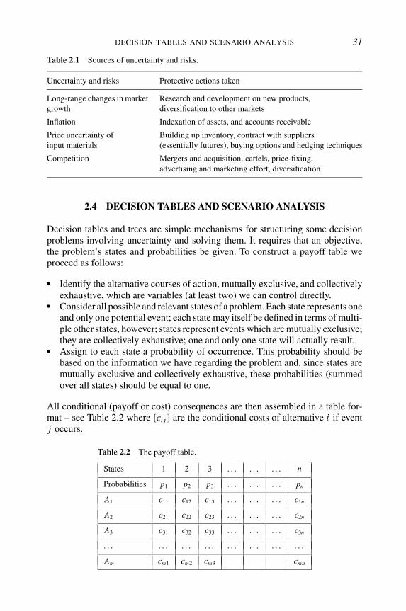
DECISION TABLES AND SCENARIO ANALYSIS 31
Table 2.1 Sources of uncertainty and risks.
Uncertainty and risks Protective actions taken
Long-range changes in marketgrowth
Research and development on new products,diversification to other markets
Inflation Indexation of assets, and accounts receivable
Price uncertainty ofinput materials
Building up inventory, contract with suppliers(essentially futures), buying options and hedging techniques
Competition Mergers and acquisition, cartels, price-fixing,advertising and marketing effort, diversification
2.4 DECISION TABLES AND SCENARIO ANALYSIS
Decision tables and trees are simple mechanisms for structuring some decisionproblems involving uncertainty and solving them. It requires that an objective,the problem’s states and probabilities be given. To construct a payoff table weproceed as follows:
Identify the alternative courses of action, mutually exclusive, and collectivelyexhaustive, which are variables (at least two) we can control directly.
Consider all possible and relevant states of a problem. Each state represents oneand only one potential event; each state may itself be defined in terms of multi-ple other states, however; states represent events which are mutually exclusive;they are collectively exhaustive; one and only one state will actually result.
Assign to each state a probability of occurrence. This probability should bebased on the information we have regarding the problem and, since states aremutually exclusive and collectively exhaustive, these probabilities (summedover all states) should be equal to one.
All conditional (payoff or cost) consequences are then assembled in a table for-mat – see Table 2.2 where [ci j ] are the conditional costs of alternative i if eventj occurs.
Table 2.2 The payoff table.
States 1 2 3 . . . . . . . . . n
Probabilities p1 p2 p3 . . . . . . . . . pn
A1 c11 c12 c13 . . . . . . . . . c1n
A2 c21 c22 c23 . . . . . . . . . c2n
A3 c31 c32 c33 . . . . . . . . . c3n
. . . . . . . . . . . . . . . . . . . . . . . .
Am cm1 cm2 cm3 cmn

32 MAKING ECONOMIC DECISIONS UNDER UNCERTAINTY
For example, for a credit manager, what are the relevant states to considerwhen a customer comes in and demands a loan? Simply grant the loan (state 1)or not (state 2). If the loan is not reimbursed on time (and reimbursement delaysare introduced) there may be other ways to express these states. For example,a first state would stand for no delay, a second, would stand for a one-perioddelay, a third state for a two-period delay, and so on. The entries in the table tellus what will be the conditional payoffs (or costs) associated with each action.The sample Table 2.2 specifies n states 1, 2, 3, 4, . . . n and m alternatives. Whenalternative Ai , i = 1, 2, . . . , m is taken and say state j occurs with probabilityp j , j = 1, 2, . . . , n, then the cost (or payoff) is ci j (orπi j ). Thus, in such a decisionproblem, there are:
(1) n potential, mutually exclusive and exhaustive states,(2) m alternative actions, one of which only can be selected,(3) nm conditional consequences we should be able to define.
If we use an expected cost (or expected payoff) criterion, then the decision selectedwould be the one yielding the least expected cost (or, equivalently, the largestexpected payoff). The expected monetary cost of alternative i is then:
EMCi =n∑
j=1
pi j ci j
while the least cost alternative k selected is:
k ∈ Mini∈[1,..n] EMCi ProblemCash management consists of managing the short-term flow of funds in order tomeet a potential need or demand for cash. Cash is kept primarily because of itsneed in the future. Assume, for example, that an investor has the following needsfor money:
Quantities 100 300 500 700 900
Probabilities 0.05 0.25 0.50 0.15 0.05
(1) What are the potential courses of action?(2) What are the problem states? And their probabilities?(3) What are the conditional costs if the bank rate is 20 % yearly?
2.4.1 The opportunity loss table
Say that action i has been selected and event j occurs and thus payoff πi j is gained.If we were equipped with this knowledge prior to making a decision, it is possiblethat another decision would bring greater profits. Assume such knowledge andlet the maximum payoff, based on the best decision be
Maxj
[πi j ]

EMV, EOL, EPPI, EVPI 33
Table 2.3 Opportunity loss table.
States 1 2 3 . . . . . . . . . n
Probabilities p1 p2 p3 . . . . . . . . . pn
A1 l11 l12 l13 . . . . . . . . . l1n
A2 l21 l22 l23 . . . . . . . . . l2n
A3 l31 l32 l33 . . . . . . . . . l3n
. . . . . . . . . . . . . . . . . . . . . . . .
Am lm1 lm2 lm3 lmn
The difference between this maximum payoff and the payoff obtained by takingany other decision is called the opportunity loss, denoted by:
li j = Maxj
[πi j ] − πi j
The opportunity loss table is therefore a matrix as given in Table 2.3.Thus, the opportunity loss is the difference between the costs or profits actually
realized and the costs or profits which would have been realized if the decisionhad been the best one possible. A project might seem like a good investment, butit means that we have lost the opportunity to do something else that might be moreprofitable. This loss may be likened to the additional income a trader would haverealized had he been an inside trader, benefiting from information regarding stockprices before they reach the market! As a result, we can verify that the differencebetween the expected profits of any two acts is equal in magnitude but oppositein sign to the difference between their expected losses. By the same token, thedifference between the expected costs of any two acts is equal in magnitudeand identical in sign to the difference between their expected opportunity losses.With these definitions on hand we can also state that: the cost of uncertainty is theexpected opportunity loss of the best possible decision under a given probabilitydistribution.
2.5 EMV, EOL, EPPI, EVPI
EMV, EOL, EPPI and EVPI are terms associated with a decision; they will beelucidated through an application. Assume that data supplied by a Port Authoritypoints to a number of development alternatives for the port. Uncertainty regard-ing the economic state of the country, geopolitical developments and so on, leadto a number of scenarios to be considered and against which each of these al-ternatives must be assessed. Each alternative can generate, ex-post, a sense ofsatisfaction at having followed the proper course of action as well as a sense thata suboptimal alternative was taken. Four scenarios are assumed each to lead tothe following results, summarized in the table below where entries are payoffs(losses):

34 MAKING ECONOMIC DECISIONS UNDER UNCERTAINTY
Scenario 1 2 3 4 5 6
Probability 0.1 0.15 0.25 0.05 0.3 0.15
Alternative 1 –200 –100 150 400 –300 700
Alternative 2 300 –150 300 600 100 500
Alternative 3 –500 300 400 –100 400 100
Alternative 4 400 600 –100 –250 –300 100
2.5.1 The deterministic analysis
An alternative is selected irrespective of the probabilities of forthcoming events.Given a number of alternatives and specified events, a decision can be taken. Anumber of criteria are used, such as maximax, maximin, minimax regret and the‘equally likely’ (Laplace) criteria as stated earlier. Under these criteria, we seethat alternatives 1 and 2 are always better than alternatives 3 and 4. Explicitly, thefollowing results are obtained:
Criterion Decision Payoff
Maximax Alternative 1 700
Maximin Alternative 2 −150
Minimax regret Alternative 1 700
Equally likely Alternative 2 275
2.5.2 The probabilistic analysis
Probabilistic analysis characterizes the likelihood of forthcoming events by asso-ciating a probability with each event. It uses a number of potential criteria but weshall be concerned essentially with the EMV – expected monetary value index ofperformance. The results for our example are given by the following:
Probabilistic analysis: The Port AuthorityExpected value – Summary reportDecision Expected payoffAlternative 1 37.50Alternative 2 217.50Alternative 3 225.00 *Alternative 4 17.50
Calculations were made as follows:Alternative 1: 0.1(−200) + 0.15(−100) + 0.25(150) + 0.05(400) + 0.3(−300) + 0.15(700) = 37.50Alternative 2: 0.1(300) + 0.15(−150) + 0.25(300) + 0.05(600) + 0.3(100) + 0 .15(500) = 217.50Alternative 3: 0.1(−500) + 0.15(300) + 0.25(400) + 0.05(−100) + 0.3(400) + 0.15(100) = 225.00Alternative 4: 0.1(400) + 0.15(600) + 0.25(−100) + 0.05(−2500) + 0.3(−300) + 0.15(100) = 17.50

EMV, EOL, EPPI, EVPI 35
The EMV (expected monetary value) consists of valuing each alternative by itsEMV. The ‘best’ choice (in an EMV context) is 225. In other words, ex-ante, thebest decision we can take is alternative 3. By contrast, if a decision could be takenex-post, once uncertainty is revealed and removed, the cost of each decision isgiven by its opportunity loss, whose expectation is the EOL (expected opportunityloss). This value is calculated explicitly through the opportunity loss table below:
Table of opportunity losses, calculations
Scenario 1 2 3 4 5 6
Probability 0.1 0.15 0.25 0.05 0.3 0.15
Alternative 1 400 − ( −200) 600 − ( −100) 400 − 150 600 − 400 400 − ( −300) 700 − 700
Alternative 2 400 − 300 600 − ( −150) 400 − 300 600 − 600 400 − 100 700 − 500
Alternative 3 400 − ( −500) 600 − 300 400 − 400 600 − ( −100) 400 − 400 700 − 100
Alternative 4 400 − 400 = 0 600 − 600 400 − ( −100) 600 − ( −250) 400 − ( −300) 700 − 100
Table of opportunity losses
Scenario 1 2 3 4 5 6
Probability 0.1 0.15 0.25 0.05 0.3 0.15
Alternative 1 60 105 62.5 10 210 0
Alternative 2 10 110.5 25 0 90 30
Alternative 3 90 45 0 35 0 90
Alternative 4 0 0 125 42.5 210 90
Entries are calculated as follows. Say that scenario 1 realizes itself. The bestalternative would then be alternative 4 yielding a payoff of 400. We replace inthe table the entry 400 by 0 and then calculate in the first column correspondingto Scenario 1 the relative losses had we selected a suboptimal alternative. Nowcompute for each alternative the expected opportunity loss, which is the sumof columns for each row. Verify that the sums EMV + EOL are equal for eachalternative, called the EPPI, or the Expected Profit under Perfect Information.Further, note that the recommended alternative under an EOL criterion is alsoalternative 3 as in the expected payoff (EMV) case. This is always the case andshould not come as any surprise, since selecting the largest EMV is equivalent tothe smallest EOL. Since,
EMV + EOL = EPPI
Note that the EOL for the third alternative equals 260 and, therefore, note thatthe EPPI is 485, which is the same for all alternatives. The EPPI means that if,ex-post, we always have the best alternative, then in expectation our payoff wouldbe 485. Since, ex-ante, it is only 225 (=EMV), the potential for improving theex-ante payoff EMV by better forecasts of the scenarios, by a better managementof uncertainty (through contracts of various sorts that manage risk) cannot belarger than the EOL or 260. Such an approach would be slightly more complex if

36 MAKING ECONOMIC DECISIONS UNDER UNCERTAINTY
we were to introduce sample surveys, information guesses etc. used to improveour assessment of the states, the probabilities and the economic value of such anassessment.
Optimal Decision: Alternative 3; Expected payoff : 225.00Probabilistic analysisExpected value of perfect information
State Prob. Decision Payoff Prob.*PayoffScenario 1 0.1000 Alternative 4 400.00 40.00Scenario 2 0.1500 Alternative 4 600.00 90.00Scenario 3 0.2500 Alternative 3 400.00 100.00Scenario 4 0.0500 Alternative 2 600.00 30.00Scenario 5 0.3000 Alternative 3 400.00 120.00Scenario 6 0.1500 Alternative 1 700.00 105.00
Expected payoff with perfect information (EPPI) 485.00Expected payoff without perfect information (EMV) 225.00Expected value of perfect information (EVPI) 260.00
If we integrate other sources of information, it is possible to improve the prob-ability estimates and, therefore, improve the optimal decision. The value of in-formation, of a sample on the basis of which such information is available, iscalled EVSI (or the expected value of sample information). It is a gain obtainedby improving our assessment of the events/states probabilities. Finally, if gainsand losses are weighted in a different manner, then we are led to approaches basedon disappointment (giving greater weight to losses, relative to gains) and elation(when the prospects of ‘doing better than expected’ is more valued because of theself-gratification it produces). Avoidance of losses, motivated by disappointment,can also lead to selecting alternatives that have smaller gain expectation but re-duce the probability of having made the ‘wrong choice’, in the sense of ending thedevelopment project with losses. We shall return to this approach in Chapter 3.
ProblemThe Corporate Financial Officer Vice of HardKoor Co. has the problem of raisingsome additional capital. To do so, it is possible to sell 10 000 convertible bonds.A preliminary survey of the capital market indicates that they could be sold at thepresent time for $100 per bond. However, the company is currently engaged in aunion contract dispute and there is a possibility of a strike. If the strike were totake place, the selling price of the bonds would be decreased by 20 %. There isalso a possibility of winning a large, exclusive contract which, if obtained, wouldmean the bonds could be sold for 30 % more. The VP Finance would like to raisethe maximum amount of capital, and so must decide whether to offer the bondsnow or wait for the situation to become clearer.
(a) What are the alternatives?(b) What are the sources and the types of uncertainty?(c) What action should be taken if an EMV criterion is used? – if a minimax
criterion is taken? – if a maximin criterion is taken? – if a regret criterion istaken?

EMV, EOL, EPPI, EVPI 37
(d) If the probability of a strike is felt to be 0.4, while the probability of thecontract being awarded is 0.8, what action is best if the EMV criterion isapplied (note that it is necessary to calculate the proceeds for the variousoutcomes), and if the expected opportunity loss (EOL) criterion is used?
(e) Give one example of how the principle of bounded rationality was apparentlyused in formulating the problem?
SELECTED REFERENCES AND READINGS
Bell, D.E. (1982) Regret in decision making under uncertainty, Operations Research, 30, 961–981.
Bell, D.E. (1983) Risk premiums for decision regrets, Management Science, 29, 1156–1166.Loomes, G., and R. Sugden (1982) Regret theory: An alternative to rational choice under
uncertainty, Economic Journal, 92, 805–824.Loomes, G., and R. Sugden (1987) Some implications of a more general form of regret theory,
Journal of Economic Theory, 41, 270–287.Luce, R.D., and H. Raiffa (1958) Games and Decisions, John Wiley & Sons, Inc., New York.Raiffa, H., and R. Schlaiffer (1961) Applied Statistical Decision Theory, Division of Research,
Graduate School of Business, Harvard University, Boston, MA.Rubinstein, A. (1998) Modeling Bounded Rationality, MIT Press, Boston, MA.Savage, L.J. (1954) The Foundations of Statistics, John Wiley & Sons, Inc., New York.Winkler, R.L. (1972) Introduction to Bayesian Inference and Decision, Holt, Rinehart & Win-
ston, New York.

CHAPTER 3
Expected Utility
3.1 THE CONCEPT OF UTILITY
When the expected monetary value (EMV) is used as the sole criterion to reacha decision under uncertainty, it can lead to results we might not have intended.Outstanding examples to this effect are noted by observing people gambling in acasino or acquiring insurance. For example, in Monte Carlo, Atlantic City or LasVegas, we might see people gambling (investing!) their wealth on ventures (such asputting $100 on number 8 in roulette), knowing that these ventures have a negativeexpected return. To explain such an ‘irrational behaviour’, we may argue that notall people value money evenly. Alternatively we may rationalize that the prospectof winning 36 ∗ 100 = $3600 in a second at the whim of the roulette is worthtaking the risk. After all, someone will win, so it might as well be me! Both anattitude towards money and the willingness to take risks, originating in a person’sinitial wealth, emotional state and the pleasure to be evoked in some way by suchrisk, are reasons that may justify a departure from the Bayes EMV criterion. Ifall people were ‘straight’ expected payoff decision-makers, then there would beno national lotteries and no football or basketball betting. Even the mafia mightbe much smaller! People do not always use straight expected payoffs to reachdecisions, however. The subjective valuation of money and people’s attitudestowards risk and gambling provide the basic elements that characterize gamblingand the utility of money associated with such gambling. Utility theory seeks torepresent how such subjective valuation of wealth and attitude towards risk canbe quantified so that it may provide a rational foundation for decision-makingunder uncertainty.
Just as in Las Vegas we might derive ‘pleasure from gambling’, we may be alsoconcerned by the loss of our wealth, even if it can happen with an extremely smallprobability. To protect ourselves from large losses, we often turn to insurance.Do we insure our house against fire? Do we insure our belongings against theft?Should we insure our exports against currency fluctuations or against default pay-ment by foreign buyers? Do we invest in foreign lands without seeking insuranceagainst national takeovers? And so on. In these situations and in order to avoidlarge losses, we willingly pay money to an insurance firm – the premium neededto buy such insurance. In other words, we transfer our risk to the insurer who in
Risk and Financial Management: Mathematical and Computational Methods. C. TapieroC© 2004 John Wiley & Sons, Ltd ISBN: 0-470-84908-8

40 EXPECTED UTILITY
(
π)0: −π
( ): R R −πFigure 3.1 A lottery.
turn makes money by collecting the premium. Of course, how much premium topay for how much risk insured underscores our ability to sustain a great loss andour attitude towards risk. Thus, just as our gambler was willing to pay a smallamount of money to earn a very large one (albeit with a very small probability),we may be willing to pay a small amount (the premium) to prevent and protectourselves from having to face a large loss, even if it occurs with a very smallprobability. In both cases, the Bayes expected payoff (EMV) criterion breaksdown, for otherwise there would be no casinos and no insurance firms. Yet, theyare here and provide an important service to society. Due to the importance ofutility theory to economics and finance, providing a normative framework fordecision-making under uncertainty and risk management, we shall outline its ba-sic principles. Subsequently, we shall see how the concepts of expected utilityhave been used importantly in financial analysis and financial decision-making.
3.1.1 Lotteries and utility functions
Lotteries consist of the following: we are asked to pay a price π (say it is $5)for the right to participate in a lottery and earn, potentially, another amount, R,
called the reward (which is say $1 000 000), with some probability, p. If we do notwin the lottery, the loss is π . If we win, the payoff is R. This lottery is representedgraphically in Figure 3.1 where all cash expenditures are noted. Lotteries of thissort appear in many instances. A speculator buys a stock expecting to make aprofit (in probability) or losing his investment. Speculators are varied, however,owning various lotteries and possessing varied preferences for these lotteries. Itis the exchange between speculators and investors that create a ‘financial market’which, once understood, can provide an understanding and a valuation of lotteriespricing.
If we use an EMV criterion for valuing the lottery, as seen in the previouschapter, then the value of the lottery would be:
Expected value of lottery = p(R − π ) − (1 − p)π = pR − π < 0
By participating in the lottery, we will be losing money in an expected sense.In other words, if we had ‘an infinite amount of money’ and were to play thelottery forever, then in the long run we would lose $(π − pR)! Such odds forlotteries are not uncommon, and yet, however irrational they may seem at first,many people play such lotteries. For example, people who value the prospectof ‘winning big’ even with a small probability much more than the prospect of

THE CONCEPT OF UTILITY 41
‘losing small’ even with a large probability, buy lottery tickets. This unevenvaluation of money means that we may not be able to compare two sums ofmoney easily. People are different in many ways, not least in their preferencesfor outcomes that are uncertain. An understanding of human motivations anddecision making is thus needed to reconcile observed behaviour in a predictableand theoretical framework. This is in essence what expected utility theory isattempting to do. Explicitly, it seeks to define a scale that values money by somefunction, called the utility function U (.), whose simple expectation provides thescale for comparing alternative financial and uncertain prospects. The larger theexpected utility, the ‘better it is’.
More precisely, the function U (.) is a transformation of the value of money thatmakes lotteries of various sums comparable. Namely, the two sums (R − π ) and(−π ), can be transformed into U (R − π ) and U (−π ), and then the lottery wouldbe,
Make U (R − π ) with a probability p. Make (lose) U (−π ) with a probability 1 − p.
while its expected value, which tells how valuable it is compared to other lotteries,is:
Expected utility = EU = pU (R − π ) + (1 − p)U (−π )
This means that:
If EU = 0, we are indifferent whether we participate in the lottery or not. If EU > 0, we are better off participating in the lottery. If EU < 0, we are worse off participating in the lottery.
Thus, participation in a lottery is measured by its expected utility. Further, theprice $π we will be willing to pay – the premium, for the prospect of winning $Rwith probability p – is the price that renders the expected utility null, or EU = 0,found by the solution to
EU = 0 = pU (R − π ) + (1 − p)U (−π )
which can be solved for π when the utility function is specified.By the same token, expected utility can be used by an investor to compare
various lotteries, various cash flows and payments, noting that the value of eachhas an expected utility, known for certain and used to scale the uncertain prospects.The ‘expected utility’ approach to decision-making under uncertainty is thusextremely useful, providing a rational approach ‘eliminating the uncertainty fromdecision-making’ and bringing it back to a problem under certainty, which we cansolve explicitly and numerically. But there remains the nagging question: how canwe obtain such utility functions? And how justified are we in using them? VonNeumann and Morgenstern, two outstanding mathematicians and economists,concluded in the late 1940s, that for expected utility to be justified as a scalingfunction for uncertain prospects the following holds:

42 EXPECTED UTILITY
(1) The higher the utility the more desirable the outcome. This makes it possibleto look for the best decision by seeking the decision that makes the expectedutility largest.
(2) If we have three possibilities (such as potential investment alternatives), thenif possibility ‘1’ is ‘better’ than ‘2’ and ‘2’ is better than ‘3’, then necessarily‘1’ is better than ‘3’. This is also called the transitivity axiom.
(3) If we are indifferent between two outcomes or potential acts, then necessarilythe expected utilities will be the same.
These three assumptions, underlie the rational framework for decision makingunder uncertainty that expected utility theory provides.
3.2 UTILITY AND RISK BEHAVIOUR
An expected utility provides a quantitative expression of a decision makers’ de-sires for higher rewards as well as his attitude towards the ‘risks’ of such rewards.Say that R, P(.) is a set of rewards R assumed to occur with probability P(.) andlet u(.) define a utility function. The basic utility theorem states that the expectedutility provides an objective index to evaluate the desirability of rewards, or:
E (u(R)) =∫
u(R)P(R) dR; R ∈
Given uncertain prospects, a rational decision-maker will then select that prospectwhose expected utility is largest. For example, the EU of an alternative prospecti with probability outcomes (πij, pij) is:
EUi =n∑
j=1
piju(πij)
and the optimal alternative k is found by:
k ∈ Maxi∈[1,n] EUi In this decision approach, the function u(.), stands for the investor’s psychology.For example, we might construe that u′(.) > 0 implies greed, u′′(.) < 0 impliesfear, while risk tolerance and prudence are implied by the signs of the thirdderivative u′′′(.) > 0 and u′′′(.) < 0 respectively. Given a probability distributionfor rewards, P(R), the basic assumptions regarding continuous utility functionsare that alternative rewards:
(1) can be compared (comparability).(2) can be ranked such that preferred alternatives have greater utility.(3) have strong independence.(4) have transitive preferences (transitivity).(5) are indifferent if their utilities are equal.

UTILITY AND RISK BEHAVIOUR 43
3.2.1 Risk aversion
Expected utility provides an investor preference for uncertain payoffs, expressingthereby his attitude toward the risk associated with such payoffs. Three attitudesare defined: (1) risk aversion (2) risk loving and (3) risk neutrality. Risk aversionexpresses a risk-avoidance preference and thus a preference for more conservativegambles. For example, a risk-averse investor may be willing to pay a premium toreduce risk. A risk lover would rather enjoy the gamble that an investment riskprovides. Finally, risk neutrality implies that rewards are valued at their objectivevalue by the expectation criterion (EMV). In other words, the investor would beoblivious to risk. For risk-averse investors, the desire for greater rewards withsmaller probabilities will decrease (due to the increased risk associated with suchrewards); such an attitude will correspond to a negative second derivative of theutility function or equivalently to an assumption of concavity, as we shall seebelow. And, vice versa, for a risk loving decision-maker the second derivative ofthe utility function will be positive. To characterize quantitatively a risk attitude,two approaches are used:
Risk aversion directly relates to the risk premium, expressed by the differencebetween the expected value of a decision and its certainty (riskless) equivalentreward.
Risk aversion is expressed by a decreasing preference for an increased risk,while maintaining a mean preserving spread.
These two definitions are equivalent for concave utility functions, as we shall seebelow.
Certainty equivalence and risk premiumAssume an uncertain reward R whose expected utility is E(u(R)). Its equivalentsure amount of money, given by the expected utility of that amount, is called thecertainty equivalent which we shall denote here by R and is given by
u(R) = E(u(R)) and R = u−1E[u(R)]Note that the certainty equivalent is not equal to the expected value R = E(R) forit embodies as well the cost of risk associated with the uncertain prospect valuedby its expected utility. The difference ρ = R − R, expresses the risk premium adecision maker would be willing to pay for an outcome that provides for sure theexpected return compared to the certainty equivalent. It can be null, positive ornegative. In other words, the risk premium is:
Risk premium (ρ) = Expected return (R) − The certainty equivalent (R)
An alternative representation of the risk premium can be reached by valuing theexpected utility of the random payoff: R = R + ε where E(ε) = 0, var(ε) = σ 2
and σ 2 denotes the payoff spread. In this case, note that a Taylor series expansion

44 EXPECTED UTILITY
around the mean return yields:
Eu(R) = Eu(R + ε) = u(R) + σ 2 u′′(R)
2
Similarly, a first-order Taylor series expansion of the certainty equivalent utilityaround the mean return (since there are no uncertain elements associated with it)yields:
u(R) = u(R − ρ) = u(R) − ρu′(R)
Equating these two equations, we obtain the risk premium calculated earlier butexpressed in terms of the derivatives of the utility function and the return variance,or:
ρ = −1
2σ 2 u′′(R)
u′(R)
This risk premium can be used as well to define the index of risk behavioursuggested by Arrow and Pratt. In particular, Pratt defines an index of absolute riskaversion expressing the quantity by which a fair bet must be altered by a risk-averse decision maker in order to be indifferent between accepting and rejectingthe bet. It is given by:
ρa(R) = ρ
σ 2/2= −u′′(R)
u′(R)
Prudence and robustnessWhen a decision-maker’s expected utility is not (or is mildly) sensitive to othersources of risk, we may state that the expected utility is ‘robust’ or expressesa prudent attitude by the decision-maker. A prudent investor, for example, whoadopts a given utility function to reach an investment decision, expresses both hisdesire for returns and the prudence he hopes to assume in obtaining these returns,based on the functional form of the utility function he chooses. Thus, an investorwith a precautionary (prudence) motive will tend to save more to hedge againstthe uncertainty that arises from additional sources of risk not accounted for bythe expected utility of uncertain returns. This notion of prudence was first definedby Kimball (1990) and Eeckoudt and Kimball (1991) and is associated withthe optimal utility level (measured by the relative marginal utilities invariance),which is, or could be, perturbed by other sources of risk. Explicitly, say that(w, R) is the wealth of a person and the random payoff which results from someinvestment. If we use the expected marginal utility, then at the optimum investmentdecision:
Eu′(w + R) > u′(w) if u′ is convex
Eu′(w + R) < u′(w) if u′ is concave
The risk premium ψ that the investor pays for ‘prudence’ is thus the amount ofmoney required to maintain the marginal utility for sure at its optimal wealth

UTILITY AND RISK BEHAVIOUR 45
level. Or:
u′(w − ψ) = Eu′(w + R) and ψ = w − u′−1[Eu′(w + R)]
Proceeding as before (by using a first term Taylor series approximation on themarginal utility), we find that:
ψ = 1
2var(R)
[−u′′′(w)
u′′(w)
]
The square bracket term is called the degree of absolute prudence. For a risk-averse decision maker, the utility second-order derivative is negative (u′ ≤ 0) andtherefore prudence will be positive (negative) if the third derivative u′′′ is positive(negative). Further, Kimball also shows that if the risk premium is positive anddecreases with wealth w, then ψ > π . As a result, ψ − π is a premium an investorwould pay to render the expected utility of an investment invariant under othersources of risks.
The terms expected utility, certainty equivalent, risk premium, Arrow–Prattindex of risk aversion and prudence are used profusely in insurance, economicsand financial applications, as we shall see later on.
3.2.2 Expected utility bounds
In many instances, calculating the expected utility can be difficult and thereforebounds on the expected utility can be useful, providing a first approximation to theexpected utility. For risk-averse investors with utility function u(.) and u′′(.) ≤ 0,the expected utility has a bound from above, known as Jensen’s inequality. It isgiven by:
Eu(R) ≤ u(R) when u′′(.) ≤ 0
Eu(R) ≥ u(R) when u′′(.) ≥ 0
and vice versa when it is the utility function of a risk-loving investor (i.e. u′′(.) ≥0). When rewards have known mean and known variance however, Willasen(1981, 1990) has shown that for risk-averse decision-makers, the expected utilitycan be bounded from below as well. In this case, we can bound the expectedutility above and below by:
u(R) ≥ Eu(R) ≥ R2u(α2/R)/α2; α2 = E(R2)
The first bound is, of course, Jensen’s inequality, while the second inequalityprovides a best lower bound. It is possible to improve on this estimate by usingthe best upper and lower Tchebycheff bounds on expected utility (Willasen, 1990).This inequality is particularly useful when we interpret and compare the effectsof uncertainty on the choice of financial decisions, as we shall see in the examplebelow. Further, it is also possible to replace these bounds by polynomials suchthat:
Eu(R) ≤ E A(R); Eu(R) ≥ E B(R)

46 EXPECTED UTILITY
where A(.) and B(.) are polynomials of the third degree. To do so, second- andthird-order Taylor series approximations are taken for the utility functions (usingthereby the decision-makers’ prudence). For example, consider the followingportfolio prospect with a mean return of R and a variance σ 2. Say that meanreturns are also a function of the variance, expressing the return-risk substitution,with:
R = R(σ ), ∂ R(σ )/∂σ>, R(0) = R f
where R f denotes the riskless rate of return. It means that the larger the returnsuncertainty, the larger the required expected payoff. Using the Jensen and Willaseninequalities, we have for any portfolio, the following bounds on the expectedutility:
u(R(σ )(1 + ν))
1 + ν≤ Eu(R) ≤ u(R(σ )); ν=σ 2
R2; E(R2) = R2 + σ 2
Thus, lower and upper bounds of the portfolio expected utility can be constructedby maximizing (minimizing) the lower (upper) bounds over feasible (R, σ ) port-folios. Further, if we set R = R f + λσ where λ is used as a measure for the price ofrisk (measured by the return standard deviation and as we shall see subsequently),we have equivalently the following bounds:
u((R f + λσ )(1 + ν))
1 + ν≤ Eu(R) ≤ u(R f + λσ )
The definition of an appropriate utility function is in general difficult. For thisreason, other means are often used to express the desirability of certain outcomes.For example, some use targets, expressing the desire to maintain a given level ofcash, deviations from which induce a dis-utility. Similarly, constraints (as they aredefined by specific regulation) as well as probability constraints can also be usedto express a behavioural attitude towards outcomes and risks. Such an approachhas recently been found popular in financial circles that use ‘value at risk’ (VaR)as an efficiency criterion (see Chapter 10 in particular). Such assumptions re-garding decision-makers’ preferences are often used when we deal with practicalproblems.
3.2.3 Some utility functions
A utility function is selected because it represents the objective of an investorfaced with uncertain payoffs and his attitude towards risk. It can also be selectedfor its analytical convenience. In general, such a selection is difficult and hastherefore been one of the essential reasons in practice for seeking alternativeapproaches to decision making under uncertainty. Below we consider a numberof analytical utility functions often used in theoretical and practical applications.
(1) The exponential utility function: u(w) = 1 − e−aw, a > 0 is a concavefunction. For this function, u′(w) = a e−aw > 0, u′′(w) = −a2 e−aw < 0 whilethe index of absolute risk aversion RA is constant and given by: RA(w)

UTILITY AND RISK BEHAVIOUR 47
= −u′′/u′ = a > 0. Further u′′′(w) = a3 e−aw > 0 and therefore the degree ofprudence is a while the prudence premium is, ψ = 1
2 a var(R).(2) The logarithmic utility function: u(w) = log(β + γw), with β > 0, γ > 0
is strictly increasing and strictly concave and has a strictly decreasing absoluterisk aversion. Note that, u′(w) = γ /(β + γw) > 0, u′′(w) = −γ 2/(β + γw)2 <
0 while, RA(w) = γ /(β + γw) = u′(w) which is decreasing in wealth.(3) The quadratic utility function: u(w) = w − ρw2 is a concave function for
all ρ ≥ 0 since u′ = 1 − 2ρw, u′ ≥ 0 → w ≤ 1/2ρ and u′′ = −2ρ ≤ 0. As aresult, the Arrow–Pratt index of absolute risk aversion is
RA(w) = −u′′[E(w)]
u′[E(w)]= 2ρ
1 − 2ρw
and the prudence is null (since the third derivative is null).(4) The cubic utility function: u(w) = w3 − 2kw2 + (k2 + g2)w, k2 > 3g2 is
strictly increasing and strictly concave and has a decreasing absolute risk aversionif 0 ≤ w ≤ 2
3 k − 12
√k2 − 3g2.
(5) The power utility function: u(w) = (w − δ)β , 0 < β < 1 is strictly increas-ing and has a strictly absolute risk aversion on [δ, ∞) since: u′ = β (w − δ)β−1 ,
and u′′ = −(1 − β)β (w − δ)β−2. The risk aversion index is thus, RA(w) =−(1 − β) (w − δ)−1.
(6) The HARA (hyperbolic absolute risk aversion) has a utility function givenby:
u(w) = 1 − γ
γ
[aw
1 − γ+ b
]γ
while its first and second derivatives as well as its index of absolute risk aversionare given by:
u′ = a
[aw
1 − γ+ b
]γ−1
> 0, u′′ = −a2
[aw
1 − γ+ b
]γ−2
< 0;
Ra(w) = −u′′
u′ = a
b + aw/(1 − γ )> 0
This utility function includes a number of special cases. In particular, when γ
tends to one, we obtain the logarithmic utility.
3.2.4 Risk sharing
Two firms sign an agreement for a joint venture. A group of small firms organizea cooperative for marketing their products. The major aerospace companies inthe US west coast set up a major research facility for deep space travel. A groupof 70 leading firms form a captive insurance firm in the Bahamas to insure theirmanagers against kidnappings, and so on. These are all instances of risk sharing.Technically, when we combine together a number of (independent) participantsand split among them a potential loss or gain, the resulting variance of the lossor gain for each of the participants will be smaller. Assuming that this variance

48 EXPECTED UTILITY
is an indicator of the ‘risk’, and if decision makers are assumed to be risk averse,then the more partners in the venture the smaller the individual risk sustained byeach partner. Such arguments underly the foundations of insurance firms (thatcreate the means for risk sharing), of major corporations based on numerousshareholders etc. Assuming that our preference is well defined by a utility functionU(.), how would we know if it is worthwhile to share risk? Say that the netbenefits (profits less costs) of a venture is $X whose probability distribution isp(X ). If we do nothing, nothing is gained and nothing is lost and therefore the‘value’ of doing nothing is U(0). The venture with its n participants, however, willhave an expected utility EU (X/n). Thus, if sharing is worthwhile the expectedutility of the venture ought to be greater than the utility of doing nothing! Or,EU (X/n) > U (0).
Problems(1) Formulate the problem of selecting the optimal size of a risk-sharing pool.(2) How much does a member of the pool benefit from participating in sharing.
3.3 INSURANCE, RISK MANAGEMENT AND EXPECTED UTILITY
How much would it be worth paying for car insurance (assuming that there issuch a choice)? This simple question highlights an essential insurance problem.If we are fully insured and the premium is $π , then the expected utility is, forsure, U (w − π ) where w is our initial wealth. If we-self-insure for a risk whoseprobability distribution is p(X ), then using the expected utility theory paradigm,we should be willing to pay a premium π as long as U (w − π ) > EU (w − X ).In fact the largest premium we would be willing to pay solves the equation above,or
π∗ = w − U−1(EU (w − X ))
Thus, if the utility function is known, we can find out the premium π∗ abovewhich we would choose to self-insure.
ProblemFor an exponential, HARA and logarithmic utility function, what is the maximalpremium an individual will be willing to pay for insurance?
3.3.1 Insurance and premium payments
Insurance risk is not reduced but is transferred from an individual to an insurancefirm that extracts a payment in return called the premium and profits from it byinvesting the premium and by risk reducing aggregation. In other words, it is thedifference in risk attitudes of the insurer and the insured, as well as the priceinsured, and insurers are willing to pay for that to create an opportunity for theinsurance business.

INSURANCE, RISK MANAGEMENT AND EXPECTED UTILITY 49
Say that X is a risk to insure (a random variable) whose density function isF(X ). Insurance firms, typically, seek some rule to calculate the premium theyought to charge policyholders. In other words, they seek a ‘rule’ ϒ such that apremium can be calculated by:
P = ϒ(F(X ))
Although there are alternative ways to construct this rule, the more prominentones are based on the application of the expected utility paradigm and traditionallybased on a factor loading the mean risk insured. The expected utility approachseeks a ‘fair’ premium P which increases the firm expected utility, or:
U (W ) ≤ EU (W + P − X )
where W is the insurance firm’s capital. The loading factor approach seeks, how-ever, to determine a loading parameter λ providing the premium to apply to theinsured and calculated by P/n = (1 + δ)E(x), where x denotes the individualrisk in a pool of n insured, i.e. x = X/n and P/n is an individual premium share.For the insured, whose utility function is u(.) and whose initial wealth is w, theexpected utility of insurance ought to be greater than the expected utility of self-insurance. As a result, a premium P is feasible if the expected utilities of both theinsurer and the insured are larger with insurance, or:
u(w − P/n) ≥ Eu(w − xi ), X =n∑
i=1
xi ; U (W ) ≤ EU (W + P − X )
Note that in this notation, the individual risk is written as xi which is assumed to beidentically and independently distributed for all members of the insurance pool.Of course, since an insurance firm issues many policies, assumed independent, itwill profit from risk aggregation. However, if risks are correlated, the variance ofX will be much greater, prohibiting in some cases the insurance firm’s ability orwillingness to insure (as is the case in natural disaster, agricultural and weatherrelated insurance).
Insurance ‘problems’ arise when it is necessary to resolve the existing dispari-ties between the insured and the insurer, which involves preferences and insuranceterms that are specific to both the individual and the firm. These lead to extremelyrich topics for study, including the important effects of moral hazard, adverseselection resulting from information asymmetry which will be studied subse-quently, risk correlation, rare events with substantive damages, insurance againsthuman-inspired terrorists acts etc.
Risk sharing, risk transfer, reinsurance and other techniques of risk managementare often used to spread risk and reduce its economic cost. For example, let xbe the insured risk; the general form of reinsurance schemes associated with aninsurer (I), an insured (i) and a reinsurer (r) and consisting in sharing risk can be

50 EXPECTED UTILITY
written as follows:
Insured: Ri (x |a , q) =
x x ≤ a(1 − q)x x ≥ a
Insurer: RI (x |a, b, c, q ) =
0 x ≤ aq(x − a) a < x ≤ b
c b > x
Reinsurer: Rr (x |b, c, q ) =
0 x ≤ bq(b − x) − c x ≥ b
Here, if a risk materializes and it is smaller than ‘a’, then no payment is madeby the insurance firm while the insured will be self-insured up to this amount.When the risk is between the lower level ‘a’ and the upper one ‘b’, then only aproportion q is paid where 1−q is a co-participation rate assumed by the insured.Finally, when the risk is larger than ‘b’, then only c is paid by the insurer whilethe remaining part x − c is paid by a reinsurer. In particular for a proportionalrisk scheme we have R(x) = qx while for an excess-loss reinsurance scheme wehave:
RI (x |a ) =
0 x ≤ ax − a x > a
where a is a deductible specified by the insurance contract. A reinsurance schemeis thus economically viable if the increase in utility is larger than the premiumPr to be paid to the reinsurer by the insurance firm. In other words, for utilityfunctions uI (.), ui (.), ur (.) for the individual, the insurance and the reinsurancefirms with premium payments: Pi , PI , Pr , the following conditions must be held:
ui (w − Ri (x |a, q ) − Pi ) ≥ Eui (w − x) (the individual condition)
uI (W ) ≤ EuI (W + Pi − PI − RI (x |a, b, c, q )) (the insurance firm condition)
ur (Wr ) ≤ Eur (Wr + PI − Rr (x |b, c, q )) (the reinsurer condition)
Other rules for premium calculation have also been suggested in the insuranceliterature. For example, some say that in insurance ‘you get what you give’. Inthis sense, the premium payments collected from an insured should equal whathe has claimed plus some small amounts to cover administrative expenses. Theseissues are in general much more complex because the insurer benefits from riskaggregation over the many policies he insures, a concept that is equivalent toportfolio risk diversification. In other words, if the insurance firm is large enough itmight be justified in using a small (risk-free) discount rate in valuing its cash flows,compared to an individual insured, sensitive with the uncertain losses associatedwith the risk insured. For this reason, the determination of the loading rate is oftena questionable parameter in premium determination. Recent research has greatlyimproved the determination of insurance premiums by indexing insurance riskto market risk and using derivative markets (such as options) to value insurancecontracts (and thereby the cost of insurance or premium).

CRITIQUES OF EXPECTED UTILITY THEORY 51
3.4 CRITIQUES OF EXPECTED UTILITY THEORY
Theory and practice do not always concur when we use expected utility theory.There are many reasons for such a statement. Are decision-makers irrational? Arethey careless? Are they uninformed or clueless? Do they lack the proper incentivesto reach a rational decision. Of course, the axioms of rationality that underlieexpected utility theory may be violated. Empirical and psychological research hassought to test the real premises of decision-makers under uncertainty. To assesspotential violations, we consider a number of cases. Consider first the examplebelow called the St Petersburg Paradox that has motivated the development of theutility approach.
3.4.1 Bernoulli, Buffon, Cramer and Feller
Daniel Bernoulli in the early 1700s suggested a problem whose solution wasnot considered acceptable in practice, albeit it seemed to be appropriate from atheoretical viewpoint. This is called the St Petersburg Paradox. The paradox isframed in a tossing game stating how much one would be willing to pay for agame where a fair coin is thrown until it falls ‘heads’. If it occurs at the r th throw,the player receives 2r dollars from the bank. Thus, the gain doubles at each throw.In an expected sense, the probability of obtaining ‘heads’ at the kth throw is 1/2k ,since the pay-out is also equal to 2k , the expected value of the game is:
∞∑
k=1
(1/2k)2k = 1 + 1 + · · · = ∞
Thus, the fair amount to pay to play this game is infinite, which clearly does notreflect the decision makers’ behaviour. Bernoulli thus suggested a logarithmicutility function whose expected utility:
Eu(x) =∞∑
i=1
p(i)u(2i−1) =∞∑
i=1
(1
2i
)log(2i−1) =
∞∑
i=1
(i − 1
2i
)log(2)
Since∞∑
i=1
(1
2i
)= 1 and
∞∑
i=1
(i − 1
2i
)= 1
The expected utility of the game equals Eu(x) = log(2).Mathematicians such as Buffon, Cramer, Feller and others have attempted to
provide a solution that would seem to be appropriate. Buffon and Cramer suggestthat the game be limited (in the sense that the bank has a limited amount of moneyand, therefore, it can only pay a limited amount). Say that the bank has only amillion dollars. In this case, we will have the following amounts,
19∑
k=1
(1/2k)2k + 106∞∑
k=20
(1/2k) = 1 + 1 + · · · 1 + 1.19 ≈ 21

52 EXPECTED UTILITY
Therefore, the fair amount to play this game is 21 dollars only. Any larger amountwould be favourable to the bank.
Gabriel Cramer, on the other hand, suggested a square root utility function.Then for the St Petersburg game, we have:
Eu(x) =∑
i=1
∞p(i)u(i) =
∞∑
i=1
(1
2i
) √2i − 1
= 1
2+
√2
22+ (
√2)2
22+ · · · + (
√2) j
2 j+1+ · · · = 1
2
1
1 − √2/2
= 1
2 − √2
And therefore, for Cramer, the value of the game is 1/(2 − √2). Feller suggests
another approach however, seeking a mechanism for the gains and payments tobe equivalent in the long run. In other words, a lottery will be fair if:
Accumulated gains
Accumulated fees= Nn
Rn→ 1 as n → ∞
or P
∣∣∣∣Nn
Rn− 1
∣∣∣∣ < ε
→ ∞ as n → ∞
Feller noted that the game is fair if Rn = n log2 (n). Thus if the accumulatedentrance fee to the game is proportional to the number of games, it will not be afair game.
3.4.2 Allais Paradox
The strongest attack on expected utility theory can be found in Allais’ Paradox,which doubts the strong independence assumption needed for consistent choicein expected utility. Allais proved that the assumption of linearity in probabilitiesapplied in calculating the expected utility is often doubtful in practice. Explicitly,the independence axiom also called the ‘sure-thing’ principle asserts that twoalternatives that have a common outcome under a particular state of nature shouldimply that ordering should be independent of the value of their common outcome.This is not always the case and counter examples abound, in particular due toAllais.
For example, let us confront people with two lotteries. First, we have to pickone of the two gambles given by (p1, p2) below. The first gamble consists of$100 000 for sure (probability 1) while the other is $5 000 000 with probability0.1, 1 million with probability 0.89 and nothing with probability 0.01 as statedbelow.
p1 ⇒ 1 100 000 and p2 ⇒
0.1 5 000 0000.89 1 000 0000.01 0
A second set of gambles (p3, p4) consists of:
p3 ⇒
0.1 5 000 0000.9 0 and p4 ⇒
0.11 1 000 0000.89 0

EXPECTED UTILITY AND FINANCE 53
Confronted with choosing between p1 and p2, people chose p1 while confrontingp1, p3 and p4, people preferred p3 which is in contradiction with the strongindependence axiom of utility theory. In other words, if gamble 1 is selectedover gamble 2, while in presenting people with gambles 1, 3 and 4 results in theirselecting 3 over 1, there is necessarily a contradiction, since if we were to comparegambles 3 and 2, clearly, 3 is not as good as 2. This contradiction means, therefore,that application of expected utility theory does not always represent investors’and decision-maker’s psychology. Since then, a large number of studies have beendone, seeking to bridge a gap between investors’ psychology and the concepts ofutility theory. Some essential references include Kahnemann and Tverski (1979),Machina on anticipated utility (1982, 1987) and Quiggin (1985) as well as manyother others. In these approaches, the expected utility framework is ‘extended’by stating that an uncertain prospect can be measured by an ‘expected utility’u(.) interpreted either as the choice of a utility function (as was the case intraditional expected utility) or by a preferred probability distribution (P) (or afunction g (P) assumed over the probability distribution). Then, the probabilitiesused to calculate the expected utility would be ‘subjective’ estimates, or beliefs,about the probabilities of returns, imbedding ‘something else’ above and beyondthe objective assessment of uncertain prospects. Thus, the objective index used tovalue the relative desirability of uncertain prospects is also a function of the modelused for probabilities P(.). This is in contrast to the utility function, expressing abehaviour imbedded in the choice of the function u(.) only, which stands solelyfor the investor’s psychology, as we saw above. For example, what if we were todetermine probabilities P∗(.) such that the price of random prospects R could beuniquely defined by the following expected value?
π =∫
R dP∗(R)
In this case, once such a well-defined transformation of these probabilities isreached, all uncertain prospects may be valued uniquely, thereby simplifyinggreatly the problem of financial valuation of risk assets such as stocks, defaultbonds and the like. This approach, defined in terms of economic exchange mar-ket mechanisms (albeit subject to specific assumptions regarding markets andindividual behaviours), underlies the modern theories of finance and ‘risk-neutralpricing’. This is also an essential topic of our study in subsequent chapters.
3.5 EXPECTED UTILITY AND FINANCE
Finance provides many opportunities for applications of expected utility. Forexample, portfolio management consists essentially of selecting an allocationstrategy among n competing alternatives (stocks, bonds, etc.), each yielding anuncertain payoff. Each stock purchase is an alternative which can lead to a (spec-ulative) profit or loss with various (known or unknown) probabilities. When se-lecting several stocks and bonds to invest in, balancing the potential gains withthe risks of losing part or all of the investment, the investor in effect constructs a

54 EXPECTED UTILITY
portfolio with a risk/reward profile which is preferred in an expected utility sense.Similarly, to evaluate projects, contracts, investments in real estate, futures andforward contracts, etc. financial approaches have been devised based directly on(or inspired by) expected utility. Below, we shall review some traditional tech-niques for valuing cash flows and thereby introduce essential notions of financialdecision making using expected utility. Typical models include the CAPM (Cap-ital Asset Pricing Model) as well the SDF (Stochastic Discount Factor) approach.
3.5.1 Traditional valuation
Finance values money and cash flow, the quantity of it, the timing of it and the riskassociated with it. A number of techniques and approaches that are subjective –defined usually by corporate financial officers or imposed by managerial require-ments – have traditionally been used. For example, let C0, C1, C2, . . . , Cn be aprospective cash flow in periods i = 1, 2, . . . , n. Such a cash flow may be knownfor sure, may be random, payments may be delayed unexpectedly, defaulted etc.To value these flows, various techniques can be used, each assuming a body ofpresumptions regarding the cash flow and its characteristics. Below, we considerfirst a number of ‘traditional’ approaches including ‘the payback period’, ‘theaccounting rate of return’ and the traditional ‘NPV’ (Net Present Value).
Payback periodThe payback period is the number of years required for an investment to berecovered by a prospective cash flow. CFOs usually specify the number of yearsneeded for recovery. For example, if 4 years is the specified time to recover aninvestment, then any project with a prospective cash flow of recovery less or equalto 4 years is considered acceptable. While, any investment project that does notmeet this requirement is rejected. This is a simple and an arbitrary approach,although in many instances it is effective in providing a first cut approach tomultiple investment opportunities. For example, say that we have an investment of$100 000 with a return cash flow (yearly and cumulatively) given by the followingtable:
Year 1 2 3 4 5 6 7 8 9
Return −5 5 10 20 40 30 20 10 10
Cumulative −5 0 10 30 70 100 120 130 140
Thus, only after the sixth year is the investment is recovered. If managementspecifies a period of 4 years payback, then of course the investment will berejected.
The accounting rate of return (ARR)The ARR is a ratio of average profit after depreciation and average investmentbook value. There are, of course, numerous accounting procedures in calcu-lating these terms, making this approach as arbitrary as the payback period.

EXPECTED UTILITY AND FINANCE 55
A decision may be made to specify a required ARR. Any such ratio ‘better’than the ARR selected would imply that the investment project is accepted.
The internal rate of return (IRR)The net present value (NPV) approach uses a discount rate R for the time valueof money, usually called the rate of return. This discount rate need not be therisk-free rate (even if future cash flows are known for sure). Instead, they arespecified by CFOs and used to provide a firm’s valuation of the prospective cashflow. Typically, it consists of three components: the real interest rate, the inflationrate and a component adjusting for investment risk.
Discount (Nominal) Rate = (Real + Inflation + Risk Compensating) Rates
Each of these rates is difficult to assess and, therefore, much of finance theoryand practice seeks to calculate these rates. The NPV of a cash flow over n periodsis given by:
NPV = C0 + C1
1 + R+ C2
(1 + R)2+ C3
(1 + R)3+ · · · + Cn
(1 + R)n
where R is the discount rate applied to value the cash flow. The IRR, however, isfound by finding the rate that renders the NPV null (NPV = 0), or by solving forR∗ is:
0 = C0 + C1
1 + R∗ + C2
(1 + R∗)2+ C3
(1 + R∗)3+ · · · + Cn
(1 + R∗)n
Each project may therefore have its own IRR which in turn can be used to rankalternative investment projects. In fact, one of the essential problems CFOs mustdeal with is selecting an IRR to enable them to select /accept investment alterna-tives. If the IRR is larger than a strategic discount factor, specified by the CFO,then investment is deemed economical and therefore can be made. There are,of course, many variants of the IRR, such as the FIE (fixed equivalent rate ofreturn) which assumes a fixed IRR with funds, generated by the investment, rein-vested at the IRR. Such an assumption is not always realistic, however, tendingto overvalue investment projects. Additional approaches based on ‘risk analysis’and the market valuation of risk have therefore been devised, seeking to evaluatethe probabilities of uncertain costs and uncertain payoffs (and thereby uncertaincash flows) of the investment at hand. In fact, the most significant attempt offundamental finance has been to devise a mechanism that takes the ‘arbitrariness’out of investment valuation by letting the market be the mechanism to value risk(i.e. by balancing supply and demand for risky assets at an equilibrium price forrisky assets). We shall turn to this important approach subsequently.
Net present value (NPV) and random cash flowsWhen cash flows are random we can use the expected utility of the randomquantities to calculate the NPV. We consider first a simple two-period example.Let C be an uncertain cash flow whose expected utility is Eu(C). Its certaintyequivalent, is CE where Eu(C) = u(CE) or CE = u−1(Eu(C)). Since CE is a sure

56 EXPECTED UTILITY
quantity, the discount rate applied to value the reception of such a quantity forone period hence is the risk free rate R f . In other words, for a one-period modelthe PV is:
PV = C E
1 + R f= u−1(Eu(C))
1 + R f= E(C) − P
1 + R f
where P is the risk premium. Equivalently we can calculate the PV by using theexpected cash flow but discounted at a rate k (incorporating the risk inherent inthe cash flow). Namely,
PV = E(C) − P
1 + R f= E(C)
1 + k
As a result, we see that the risk-free rate and the risk premium combine to deter-mine the risk adjusted rate as follows:
1 − P
E(C)= 1 + R f
1 + k→ k − R f = (1 + k)
P
E(C)or k = 1 + R f
1 − P/E(C)− 1
In particular note that k − R f defines the ‘excess discount rate’. It is the rate ofreturn needed to compensate for the uncertainty in the cash flow C . To calculate theappropriate discount rate to apply, a concept of equilibrium reflecting investors’homogeneity is introduced. This is also called ‘the capital market equilibrium’which underlies the CAPM as we shall see below. Over multiple periods of time,calculations of the PV for an uncertain future cash stream, yields similarly:
PV = C0 + E(C1)
(1 + k)1+ E(C2)
(1 + k)2+ E(C3)
(1 + k)3+ · · ·
However, interest rates (and similarly, risk-free rates, risk premiums, etc.) mayvary over time – reflecting the effects of time (also called the term structure)either in a known or unknown manner. Thus, discounting must reflect the discountadjustments to be applied to both uncertainties in the cash flow and the discountrate to apply because of the timing of payments associated with these cash flows.If the discount (interest) rates vary over time, and we recognize that each instant oftime discounting accounts for both time and risk of future cash flows, the presentvalue is then given by:
PV = C0 + E(C1)
(1 + k1)1+ E(C2)
(1 + k2)2+ E(C3)
(1 + k3)3+ · · · =
∑
i=0
E(C i )
(1 + ki )i
where k1, k2, k3, . . . , kn . . . express the term structure of the risk-adjusted rates.Finally, note that if we use the certainty cash equivalents Ci , associated with autility u(Ci ) = Eu(C i ), then:
PV =∑
i=0
Ci
(1 + R f,i )i
where R f,i is the risk-free term structure of interest rate for a discount over iperiods. In Chapter 7, we shall discuss these issues in greater detail.

EXPECTED UTILITY AND FINANCE 57
3.5.2 Individual investment and consumption
A number of issues in finance are stated in terms of optimal consumption prob-lems and portfolio holdings. Say that an individual maximizes the expected utilityof consumption, separable in time and state and is constrained by his wealth accu-mulation equation (the returns on savings and current wage income). Technically,assume that an individual investor has currently a certain amount of money in-vested in a portfolio consisting of N0 shares of a stock whose current price is p0
and a riskless investment in a bond whose current price is B0. In addition, theinvestor has a wage income of s0. Thus, current wealth is:
W0 = N0 p0 + B0 + s0
Let c0 be a planned current consumption while the remaining part W0 − c0 isreinvested in a portofolio consisting of N1 shares of a stock whose price is p0 anda bond whose current price is B1. At the next time period, time ‘1’, the investorconsumes all available income. Disposable savings W0 − c0 are thus invested ina portfolio whose current wealth is N1 p0 + B1, or initially:
W0 − c0 = N1 p0 + B1
At the end of the period, the investor’s wealth is random due to a change in thestock price p and is wholly consumed, or:
W1 = N1(p0 + p) + B1(1 + R f ) and c1 = W1
Given the investor’s utility function, there are three decisions to reach: how muchto consume now, how many shares of stock to buy and how much to invest inbonds. The problem can be stated as the maximization of:
U = u0(c0) + 1
1 + REu1(W1)
with, u0(.) and u1(.) the utilities of the current and next (final) period consumption.An individual’s preference is expressed here twice. First we use an individualdiscount rate R for the expected utility of consumption at retirement Eu1(W1).And, second, we have used the expected utility as a mechanism to express theeffects of uncertainty on the value of such uncertain payments. Define a cash(certainty) equivalent to such expected utility by C1 or C1 = u−1
1 (Eu1(W1)). Sincethis is a ‘certain cash equivalent’, we can also write in terms of cash worth:
U = C0 + C1
1 + R f, C0 = u−1
0 (u0(c0)) = c0
Note that once we have used a certain cash amount we can use the risk-free rateR f to discount that amount. As a result,
1 + R f
1 + R= u1
−1(Eu1(W1))
Eu1(W1)

58 EXPECTED UTILITY
which provides a relationship between the discounted expected utility and therisk-free discount rate for cash. Using the expected utility discount rate, we have:
U = u0(N0 p0 + B0 + s0 − N1 p0 − B1) + 1
1 + REu1(N1(p0 + p)
+B1(1 + R f ))
A maximization of the current utility provides the investment strategy (N1, B1),found by the solution of:
p0∂u0(c0)
∂ N1= 1
1 + RE
(∂u1(c1)
∂ N1(p0 + p)
),
∂u0
∂ B1= E
(∂u1
∂ B1
)
This portfolio allocation problem will be dealt with subsequently in a generalmanner but has already interesting implications. For example, if the utility ofconsumption is given by a logarithmic function, u0(c) = ln(c) and u1(c) = ln(c),we have:
p0
c0= 1
1 + RE
(p0 + p
c1
)or η0 = 1
1 + RE(η1), ηi = pi
ci, i = 0, 1
meaning that the price per unit consumption ηi is an equilibrium whose value isthe rate R. Further, the condition for the bond yields
∂u0(c0)
∂c0= E
(∂u1(c1)
∂c1
)or
1
c0= E
(1
c1
)
It implies that the current marginal utility of consumption equals the next period’sexpected marginal consumption. The investment policy is thus a solution of thefollowing two equations for (N1, B1) (where W1 = N1(p0 + p) + B1(1 + R f )):
p0
(N0 p0 + B0 + s0 − N1 p0 − B1)= 1
1 + RE
(p0 + p
W1
)
1
N0 p0 + B0 + s0 − N1 p0 − B1= E
(1
W1
)
or p0 RE(1/W1) = E( p/W1). To solve this equation numerically, we still needto specify the probability of the stock price.
ProblemAssume that
p =
H p0 w.p. π
Lp0 w.p. 1 − π
where w.p. means with probability, and find the optimal portfolio. In particular, setπ = 0.6, H=0.3, L = −0.2 and R f = 0.1, then show that the optimal investment

EXPECTED UTILITY AND FINANCE 59
policy is an all-bond investment. However, if H = 0.5, we have:
B∗1 = 0.085(N0 p0 + B0 + s0), N ∗
1 = −0.6444
(N0 + B0 + s0
p0
)
3.5.3 Investment and the CAPM
Say that an investor has an initial wealth level W0. Let k be a random rate ofreturn of a portfolio with known mean and known variance given respectively byk, σ 2
k respectively. Say that part of the individual wealth, S1, is invested in therisky asset while the remaining part B1 = W0 − S1 is invested in a non-risky assetwhose rate of return is the risk-free rate R f . The wealth one period hence is thus:
W1 = B1(1 + R f ) + S1(1 + k)
The demand for the risky asset is thus given by optimizing the expected utilityfunction:
MaxS1≥0
Eu[B1(1 + R f ) + S1(1 + k)] or MaxS1≥0
Eu[W0(1 + R f ) + S1(k − R f )]
The first two derivatives conditions are:
d(Eu(W1))
dS1= E(u′(W1)(k − R f )) = 0
d2(Eu(W1))
d(S1)2= E(u′′(W1)(k − R f )2) < 0
This is always satisfied when the investor is risk-averse. Consider the first-ordercondition, which we rewrite for convenience as follows:
E[u′(W1)k] = E[u′(W1)R f ]
By definition of the covariance, we have:
E(u′(W1)k) = k E(u′(W1)) + cov(u′(W1), k)
Thus,
k E(u′(W1)) + cov(u′(W1), k) = R f E(u′(W1))
Since the derivative of the expected utility is not null, we divide this expressionby it and obtain:
k + cov(u′(W1), k)
E(u′(W1))= R f
which clearly outlines the relationship between the expected returns of the riskyand the non-risky asset and provides a classical result called the Capital AssetPricing Model (CAPM). If we write the CAPM regression equation (to be seenbelow) by:
k = R f + β(Rm − R f )

60 EXPECTED UTILITY
then, we can recuperate the beta factor often calculated for stocks and riskyinvestments:
β = − cov(u′(W1), k)
(Rm − R f )E(u′(W1))
where Rm is the expected rate of return of a market portfolio or the stock marketindex. However, the beta found in the previous section implies:
β = cov(Rm, k)
σ 2m
= − cov(u′(W1), k)
(Rm − R f )E(u′(W1))
and therefore:
k − R f = (Rm − R f )cov(Rm, k)
σ 2m
= −cov(u′(W1), k)
E(u′(W1))
This sets a relationship between individuals’ utility of wealth, the market mech-anism and a statistical estimate of market parameters.
An equivalent approach consists in constructing a portfolio consisting of aproportional investment yi = Si/W0 in a risky asset i with a rate of return ki
while the remaining part is invested in a market index whose rate of return is Rm
(rather than investing in a riskless bond). The rate of return of the portfolio is thenk p = yi ki + (1 − yi )Rm with mean and variance:
k p = yi ki + (1 − yi )Rm, Rm = E Rm
σ 2p = y2
i σ 2i + (1 − yi )
2σ 2m + 2yi (1 − yi )σim ; σim = cov(ki , km)
where variances σ 2 are appropriately indexed according to the return variablethey represent. The returns–risk substitution is found by calculating by chaindifferentiation:
dk p
dσp= dk p/dyi
dσp/dyi
where:
dk p
dyi= ki − Rm ;
dσp
dyi= yi
(σ 2
i + σ 2m − 2σim
) + σim − σ 2m
σp
A portfolio invested only on the market index (i.e. yi = 0) will lead to:(
dσp
dxi
)
m
=(
dσp
dxi
)
xi =0
= σim − σ 2m
σpand
(dk p
dσp
)
m
= (ki − Rm)σm
σim − σ 2m
However since for all investors, the preference for returns is a linear function ofthe returns’ standard deviation, (assuming they all maximize a quadratic utilityfunction!), we have:
k = R f + λσ

EXPECTED UTILITY AND FINANCE 61
where σ is the volatility of the portfolio. For all assets we have equivalently:ki = R f + λσi and for the portfolio as well, or:
k p = R f + λσp → dki
dσi= λ and
(dk p
dσp
)
m
= (ki − Rm)σm
σim − σ 2m
and therefore,(
dk p
dσp
)
m
= (ki − Rm)σm
σim − σ 2m
= λ which leads to: ki = Rm − λσm + λσim
σm
But also Rm = R f + λσm which we insert in the previous equation, leadingthereby to a linear expression for risk discounting which assumes the form ofthe (CAPM) or:
ki = R f + λσim
σmand explicitly, ki = R f + λ cov(ki , Rm)
σm
as seen earlier. Note that this expression can be written in a form easily amenableto a linear regression in returns and providing an estimate for the βi factor:
ki = R f + βi (Rm − R f ); βi = λ cov(ki , Rm)
(Rm − R f )σm
Since λ = (Rm − R f )/σm is the market price of risk, we obtain also the followingexpression for the beta factor,
βi = cov (ki , Rm)
σ 2m
With this ‘fundamental’ identity on hand, we can calculate the risk premium ofan investment as well as the betas for traded securities.
3.5.4 Portfolio and utility maximization in practice
Market valuation of a portfolio and individual valuation of a portfolio are not thesame. The latter is based on an individual preference for the assets compositionof the portfolio and responding to specific needs. For example, denote by $Wa budget to be invested and let yi , i = 1, 2, 3, . . . , n be the dollars allocated toeach of the available alternatives with a resulting uncertain payoff
R =n∑
i=1
ri (yi )
The portfolio investment problem is then formulated by solving the followingexpected utility maximization problem:
Maximizey1,y2,y3,...,yn
Eu(R) = Eu
(n∑
i=1
ri (yi )
)subject to :
n∑
i=1
yi ≤ W, yi ≥ 0, i
= 1, 2, · · · , n

62 EXPECTED UTILITY
where u(.) is the individual utility function, providing a return risk ordering overall possible allocations. This problem has been solved in many ways. It clearlysets up a transformation of an uncertain payoffs problem into a problem which isdeterministic and to which we can apply well-known optimization and numericaltechniques. If u(.) is a quadratic utility function and the rates of return are linearin the assets allocation (i.e. ri (yi ) = ri yi ), then we have:
Maximizey1,y2,y3,...,yn
Eu(R) = Eu
(n∑
i=1
ri (yi )
)=
n∑
i=1
ri yi − µ
n∑
j=1
n∑
i=1
ρi j yi y j ;
ρi j = cov(ri , r j )
where ri is the mean rate of return on asset i, ρi j is the covariance between thereturns on two assets (i, j) and µ is a parameter expressing the investor’s riskaversion (µ > 0) or risk loving (µ < 0). This defines a well known quadraticoptimization problem that can be solved using standard computational softwarewhen the index of risk aversion is available. There are many other formulations ofthis portfolio problem due to Harry Markowitz, as well as many other techniquesfor solving it, such as scenario optimization, multi-criterion optimization andothers.
The Markowitz approach had a huge impact on financial theory and practice.Its importance is due to three essential reasons. First, it justifies the well-knownbelief that it is not optimal to put all one’s eggs in one basket (or the ‘principle ofdiversification’). Second, a portfolio value is expressed in terms of its mean returnand its variance, which can be measured by using statistical techniques. Further,the lower the correlation, the lower the risk. In fact, two highly and negativelycorrelated assets can be used to create an almost risk-free portfolio. Third andfinally, for each asset there are two risks, one diversifiable through a combinationof assets and the other non-diversifiable to be borne by the investor and for whichthere may be a return compensating this risk.
Markowitz suggested a creative approach to solving the quadratic utility portfo-lio problem by assuming a specific index of risk aversion. The procedure consistsin solving two problems. The first problem consists in maximizing the expectedreturns subject to a risk (variance) constraint (Problem 1 below) and the secondproblem consists in minimizing the risk (measured by the variance) subject to arequired expected return constraint (Problem 2 below). In other words,
Problem 1:
Maximizey1,y2,y3,...,yn
n∑
i=1
ri yi
Subject to:n∑
j=1
n∑
i=1
ρi j yi y j ≤ λ
Problem 2:
Minimizey1,y2,y3,...,yn
n∑
j=1
n∑
i=1
ρi j yi y j
Subject to:
n∑
i=1
ri yi ≥ µ
An optimization of these problems provides the efficient set of portfolios definedin the (λ, µ) plane.

EXPECTED UTILITY AND FINANCE 63
The importance of Markowitz’s (1959) seminal work cannot be overstated. Itlaid the foundation for portfolio theory whereby rational investors determine theoptimal composition of their portfolio on the basis of the expected returns, thestandard deviations of returns and the correlation coefficients of rates of return.Sharpe (1964) and Lintner (1965) gave it an important extension leading to theCAPM to measure the excess premium paid to hold a risky financial asset, as wesaw earlier.
3.5.5 Capital markets and the CAPM again
The CAPM for the valuation of assets is essentially due to Markowitz, James Tobinand William Sharpe. Markowitz first set out to show that ‘diversification pay’,in other words an investment in more than one security, provides an opportunityto ‘make money with less risk’, compared to the prior belief that the optimalinvestment strategy consists of putting all of one’s money in the ‘best basket’. Forrisk-averse investors this was certainly a strategy to avoid. Subsequently, Tobin(1956) showed that when there is a riskless security, the set of efficient portfolioscan be characterized by a ‘two-fund separation theorem’ which showed that anefficient portfolio can be represented by an investor putting some of his moneyin the riskless security and the remaining moneys invested in a representativefund constructed from the available securities. This led to the CAPM, statedexplicilty by Sharpe in 1964 and Lintner in 1965. Both assumed that investors arehomogeneous and mean-variance utility maximizers (or, alternatively, investorsare quadratic utility maximizers). These assumptions led to an equilibrium offinancial markets where securities’ risks are measured by a linear function (dueto the quadratic utility function) given by the risk-free rate and a beta multipliedby the relative returns of the ‘mutual fund’ (usually taken to be the market averagerate of return). In this sense, the CAPM approach depends essentially on quadraticutility maximizing agents and a known risk-free rate. Thus, the returns of an asseti can be estimated by a linear regression given explicitly by:
ki = αi + βi Rm + εi
where Rm is the market rate of return calculated by the rate of return of the stockmarket as a whole, βi is an asset specific parameter while εi is the statistical error.The CAPM has, of course, been subject to criticism. Its assumptions may be toostrong: for example, it implies that all investors hold the same portfolio – which isthe market portfolio, by definition fully diversified. In addition, in order to invest,it is sufficient to know the beta associated with a stock, since it is the parameterthat fully describes the asset /stock return. Considerable effort has been devotedto estimating this parameter through a statistical analysis of stocks’ risk–returnhistory. The statistical results obtained in this manner should then clarify whethersuch a theory is applicable or not. For example, for one-factor models (marketpremium in the CAPM) the following regression is run:
(k j − R f ) = α j + β j [Rm − R f ] + ε j

64 EXPECTED UTILITY
where k j is the stock (asset) j rate of return at time t, when the risk-free rate atthat time was R f , (α j , β j ) are regression parameters, while Rm is the market rateof return. Finally, ε j is the residual value, an error term, assumed to be normallydistributed with mean zero and known variance. Of course, if (α j = 0) then thiswill violate a basic assumption of no excess returns of the CAPM. In addition, Rm
must also, according to the CAPM theory, capture the market portfolio. If, again,this is not the case, then it will also violate a basic assumption of the CAPM.Using the regression equation above, the risk consists now of (assuming perfectdiversification, or equivalently, no correlation):
var(k j − R f ) = β2j σ
2m + σ 2
ε , σ 2m = var(Rm); σ 2
ε = var(ε j )
expressing risk as a summation of beta-squared times the index-market plus theresidual risk.
The problems with a one-factor model, although theory-independent (since it ismeasured by simple financial statistics), are its assumptions. Namely, it assumesthat the regression is stable and that nonstationarities and residual risks are knownas well. Further, to estimate the regression parameters, long time series are needed,which renders their estimate untimely (and, if used carefully, it is of limitedvalue). The generalization of the one-factor model into a multiple-factor modelis also known as APT, or arbitrage pricing theory. Dropping the time index, itleads to:
(k j − R f ) = α j + β j1[Rm − R f ] + · · · + β j K [RK − R f ] + ε j
where RK − R f is the expected risk premium associated with factor K . Thenumber of factors that can be used is large, including, among many others, theyield, interest-rate sensitivity, market capitalization, liquidity, leverage, labourintensity, recent performance (momentum), historical volatility, inflation, etc.This model leads also to risks defined by the matrices calculated (the orthogonalfactors of APT) using the multivariate regression above, or
Σ = B′ Γ B + Φ
where Σ is the variance–covariance matrix of assets returns, B is the matrixof assets’ exposures to the different risk factors, Γ is the vector of factor riskpremiums (i.e. in excess of the risk-free rate for period t) and finally, Φ is the(diagonal) matrix of asset residual risks. These matrices, unfortunately involvemany parameters and are therefore very difficult to estimate.
A number of approaches based on the APT are available, however. One ap-proach, the fundamental factor model assumes that the matrix B is given andproceeds to estimate the vector Γ. A second approach, called the macroeconomicapproach, takes Γ as given and estimates the matrix B. Finally, the statisticalapproach seeks to estimate (B,Γ) simultaneously. These techniques each havetheir problems and are therefore used in varying circumstances, validated by thevalidity of the data and the statistical results obtained.

EXPECTED UTILITY AND FINANCE 65
3.5.6 Stochastic discount factor, assets pricing and the Euler equation
The financial valuation of assets is essentially based on defining an approachaccounting for the time and risk of future payoffs. To do so, financial practice andtheories have sought to determine a discounting mechanism that would, appropri-ately, reflect the current value of uncertain payoffs to be realized at some futuretime. Thus, techniques such as classical discounting based on a pre-specified dis-count rate (usually a borrowing rate of return provided by banks or some otherinterest rate) were used. Subsequently, a concept of risk-adjusted discount rateapplied to discounting the mean value of a stream of payoffs was used. A par-ticularly important advance in determining an appropriate discount mechanismwas ushered in, first by the CAPM approach, as we saw above, and subsequentlyby the use of risk-neutral pricing, to be considered in forthcoming chapters. Bothapproaches use ‘the market mechanism’ to determine the appropriate discount-ing process to value an asset’s future payoffs. We shall consider these issues atlength when we seek a risk-neutral approach to value options and derivatives ingeneral. These approaches are not always applicable, however, in particular whenmarkets are incomplete and the value of a portfolio may not be determined in aunique manner. In these circumstances, attempts have been made to maintain theframework inspired by rational expectations and at the same time be consistenttheoretically and empirically verifiable. The SDF approach, or the generalizedmethod of moments, seeks to value an asset generally in terms of its future valuesusing a stochastic discount factor. This development follows risk-neutral pricing,which justified a risk-free rate discounting process with respect to some proba-bility measure, as we shall see later on (in Chapter 6).
Explicitly, the SDF approach for a single asset states that the price of an assetequals the expected value of the asset payoff, times a stochastic discount factor.This approach has the advantage that it leads to some of the classical results offinancial economics and at the same time it can be used by applying financialstatistics in asset pricing by postulating such a relationship. Define:
pt = asset price at time t that an investor may wish to buy
x t = asset returns, a random variable
mt = a stochastic discount factor to be defined below
The SDF postulates:
pt = E(mt+1 xt+1), mt+1 = 1
1 + Rt+1
where Rt+1 is a random discounting. The rationality for such a postulate is basedon the expected utility of a consumption-based model. Say that an investor hasa utility function for consumption u(.), which remains the same at times t andt + 1. We let the discount factor be ρ, expressing the subjective discount rate ofthe consumer. Current consumption is certain, while next period’s consumptionis uncertain and discounted. Thus, in terms of expected utility we have:
U (ct , ct+1) = u(ct ) + ρEt u(ct+1)

66 EXPECTED UTILITY
where Et is an expectation operator based on the information up to time t . Nowassume that st is a consumer’s salary at time t, part of which may be invested forfuture consumption in an asset whose price is pt (for example, buying stocks). Lety be the quantity of an asset bought (say a stock). Current consumption left overafter such an investment equals: ct = st − ypt . If the asst price one period hence isxt+1, then the next period consumption is simply equal to the sum of the period’scurrent income and the return from the investment, namely ct+1 = st+1 + yxt+1.As a result, the consumer problem over two periods is reduced to:
U (ct , ct+1) = u(st − ypt ) + βEt u(st+1 + yxt+1)
The optimal quantity to invest (i.e. the number of shares to buy), found by maxi-mizing the expected utility with respect to y, leads to:
∂U
∂y= −pt u
′(st − pt y) + βEt [xt+1u′(st+1 + xt+1 y)]
= −pt u′(ct ) + βEt [xt+1u′(ct+1)] = 0
which yields for an optimum portfolio:
pt = Et
[β
u′(ct+1)
u′(ct )xt+1
]
Thus, if we set the stochastic discount factor, mt+1, expressing the inter-temporalsubstitution of current and future marginal utilities of consumption, then:
mt+1 = βu′(ct+1)
u′(ct )and therefore Rt+1 =
1 − βu′(ct+1)u′(ct )
βu′(ct+1)u′(ct )
the pricing equation becomes pt = Et [mt+1 xt+1], which is the desired SDFasset-pricing equation. This equation is particularly robust and therefore itis also very appealing. For example, if the utility function is of the loga-rithmic type, u(c) = ln(c), then, u′(c) = 1/c and mt+1 = βct/ct+1, or Rt+1 =β[(1/β)ct+1 − ct ]/ct and further, pt/ct = βEt [xt+1/ct+1]. In other words, if wewrite πt = pt/ct ; πt+1 = xt+1/ct+1, then we have: πt = βEt (πt+1).
The results of such an equation can be applied to a broad a number of situations,which were summarized by Cochrane (2001) and are given in Table 3.1. Thisapproach is extremely powerful and will be considered subsequently in Chapter 8,since it is applicable to a broad number of situations and financial products. Forexample, the valuation of a call option would be (following the information inTable 3.1) given as follows (where the time index is ignored):
C = E [m Max(ST − K , 0)]
This approach can be generalized in many ways, notably by considering multipleperiods and various agents (heterogeneous or not) interacting in financial markets
Administrator
ferret

INFORMATION ASYMMETRY 67
Table 3.1 Selected examples.
Price pt Payoff xt+1
Dividend paying stock pt pt+1 + dt+1
Investment return 1 Rt+1
Price/dividend ratiopt
dt
(pt+1
dt+1+ 1
)dt+1
dt
Managed portfolio zt zt Rt+1
Moment condition E(pt zt ) xt+1zt
One-period bond pt 1
Risk-free rate 1 R f
Option C Max[ST − K , 0]
to buy, sell and transact financial assets. Cochrane (2001) in particular suggestsmany such situations. An inter-temporal framework uses the Euler conditions foroptimality to generate an equilibrium discount factor and will be considered inChapter 9.
ExampleConsider a one-dollar investment in a risk-free asset whose payoff is R f . Thus,1/
(1 + R f
) = E(m * 1) and therefore we have 1/(1 + R f ) = E(m) as expected.
3.6 INFORMATION ASYMMETRY
Uncertainty and information asymmetry have special importance because of theireffects on decision-makers. These result also in markets being ‘incomplete’ sincethe basic assumptions regarding ‘fair competition’ are violated. In general, thepresumption that information is commonly shared is also, often, violated. Someinformation may be truthful, some may not be. Truth-in-lending for example, isan important legislation passed to protect consumers, which is, in most cases,difficult to enforce. Courts are filled with litigation on claims and counter-claims,leading to a battle of experts on what the truth is and where it may lie. Envi-ronmental litigation has often led to a ‘battle of PhDs’ expounding alternativeand partial pearls of knowledge. In addition, positive, negative, informative, par-tial, asymmetric, etc. information has different effects on both decision-makersand markets. For example, firms and funds are extremely sensitive to negativeinformation regarding their stock, their products as well as their services. Phar-maceutical firms may be bankrupted upon adverse publicity, whether true or not,regarding one of their products. For example, the Food and Drug Administrationwarning on the content of benzene in Perrier’s sparkling water has more thantainted the company’s image, its bottom-line profits and, at a certain time, itsfuture prospects. Of course, the tremendous gamble Perrier has taken to meetthese claims (that were not entirely verified) is a sign of the importance Perrierattached to its reputation and to the effects of negative information.

68 EXPECTED UTILITY
Information asymmetry and uncertainty can open up the possibility of cheating,however. For example, some consumer journals may receive money in variousforms (mostly advertising dollars) not to publish certain articles and therebymanage information in a way that does not benefit the public. For this reason,regulatory authorities are needed in certain areas. A used-car salesman may betempted to sell a car with defects unknown to the prospective buyer. In somecountries, importers are not required to inform clients of the origin and the qual-ity (state) of the product and parts used in the product sold. As a result, a productclaimed to be new by the seller may not in fact be new, opening up many possibil-ities for cheating legally. These questions arise on Wall Street in many ways. Inan article in the Wall Street Journal the question was raised by Hugo Dixon withrespect to analysts’ claims and the conflict of interest when they act according totheir own edicts:
Shouldn’t analysists put their money where their mouth is? That is the contrarian response toMerrill Lynch’s decision to ban its analysts from buying shares of companies they cover. Itmight be said that researchers will have an incentive to give better opinions if they stand to makemoney if they are right – and lose money if they are wrong. Clients might also be comfortedto know that the analysts who are peppering them with ‘buy’ recommendations are followingtheir own advice. Under this contrarian position, the fact that some analysts buy shares incompanies they follow isn’t a conflict of interest all. Quite the reverse! It is an alignment ofinterests . . . this contrarian view cannot be dismissed as a piece of errant nonsense. But it isnevertheless misconceived. There is a better way of aligning analyst’s financial interests withthose of their clients. And there are potential conflicts caused by an analyst trading stocks heor she covers!
These ‘information problems’ are the subject of extensive study, both for prac-tical and theoretical reasons. A number of references are included at the endof this chapter. Below, we only consider some of the outstanding implicationsinformation asymmetry may create.
3.6.1 ‘The lemon phenomenon’ or adverse selection
In a seminal paper, Akerlof (1970) pointed out that goods of different qualities maybe uniformly priced when buyers cannot realize that there are quality differences.This is also called ‘adverse selection’ because some of the information associatedwith the choice problem may be hidden. For example, one may buy a used car, notknowing its true state, and therefore be willing to pay a price that would not trulyreflect the value of the car. In fact, we may pay an agreed-upon market price eventhough this may be a lemon. The used-car salesman may have such informationbut, for some obvious reason, he may not be amenable to revealing the true stateof the car. In such situations, price is not an indicator of quality and informedsellers can resort to opportunistic behaviour (the used-car salesman phenomenonstated above). While Akerlof demonstrated that average quality might still be afunction of price, individual units may not be priced at that level. By contrast,people who discovered in the 1980s that they had AIDS were very quick in taking

INFORMATION ASYMMETRY 69
out very large life insurance (before insurance firms knew what it really entailedand therefore were at first less informed than the insured). Bonds or stocks ofvarious qualities (but of equal ratings) are sometimes difficult to discern for anindividual investor intending to buy. For this reason, rating agencies, tracking andfollowing firms have an important role to play, compensating for the problems ofinformation asymmetry and making markets more efficient. This role is not alwaysproperly played, as evidenced by the Enron debacle, where changing accountingpractices had in fact hidden information from the public.
Information asymmetry and uncertainty can largely explain the desires of con-sumers to buy service or product warranties to protect themselves against fail-ures or to favour firms who possess service organizations (in particular whenthe products are complex or involve some up-to-date technologies). Generally intransactions between producers and suppliers, uncertainty leads to constructinglong-term trustworthy relationships and contractual engagements to assure that‘what is contracted is also delivered’. The potential for adverse selection may alsobe used to protect national markets. Anti-dumping laws, non-tariff trade barriers,national standards and approval of various sorts are some of the means used tomanage problems of adverse selection on the one hand and to manage market en-tries to maintain a competitive advantage on the other. Finance and insurance areabound with applications and examples where asymmetry induces an uncertaintywhich has nothing to do with ‘what nature does’ but with ‘what people do’.
Problems of adverse selection can sometimes be overcome by compulsoryinsurance regulation requiring all homeowners to insure their homes or requiringeveryone to take out medical insurance, for example. Some employers insure alltheir employees as one package to avoid adverse selection problems. If everyoneis insured, high-risk individuals will be better off (since they will be insured ata lower premium than justified by the risks they have in fact). Whether low-riskindividuals are better off under this scheme depends on how risk-averse they areas the insurance they are offered is not actuarially fair.
3.6.2 ‘The moral hazard problem’
For many situations, the cost of providing a product or a service depends on thebehaviour of the purchaser. For example, the cost of insurance depends on theamount of travel done by the purchaser and by the care he takes in driving. Simi-larly, the cost of warranties depends on the care of the purchaser in using the com-modity. Such behaviour cannot always be observed directly by the supplier/seller.As a result, the price cannot depend on the behaviour of the purchaser that af-fects costs. In this case, equilibrium cannot always be the first-best-optimum andsome intervention is required to reach the best solution. Questions are of course,how and how much. For example, should car insurance be obligatory? How dopurchasers react after buying insurance? How do markets behave when there ismoral hazard and how can it be compensated?
Imperfect monitoring of fund managers, for example, can lead to moral hazard.What does it mean? It implies that when the fund manager cannot be observed,there is a possibility that the provider, the fund manager, will use that fact to his

70 EXPECTED UTILITY
advantage and not deliver the right level of performance. Of course, if we contractthe delivery of a given level of returns and if the fund manager knowingly doesnot maintain the terms of the contract, he would be cheating. We can deal withsuch problems with various sorts of controls combined with incentive contracts tocreate an incentive not to cheat or lie and to perform in the interest of the investor.If a fund manager were to cheat or lie, and if he were detected, he would then bepenalized accordingly (following the terms agreed on by the contract).
For some, transparency (i.e. sharing information) is essential to provide a ‘sig-nal’ that they operate with the best of intentions. For example, some restaurantsmight open their kitchen to their patrons to convey a message of truthfulnessin so far as cleanliness is concerned. A supplier would let the buyer visit themanufacturing facilities as well as reveal procedures relating to quality, machin-ing controls and the production process in general. A fund manager will provideregulators with truthful reports regarding the fund’s state and strategy.
Moral hazard pervades some of the most excruciating problems of finance.The problem of deposit insurance and the ‘too big to fail’ syndrome encouragesexcessive risk taking. As a result of implicit governmental guarantee, banks enjoya lower cost of capital, which leads to the consistent under-pricing of credit.Swings in economic cycles are thus accentuated. The Asian financial crisis of1998 is a case in point. The extent of its moral hazard is difficult to measure butwith each bail out by governments and the IMF, the trend for excessive risk takingis reinforced.
3.6.3 Examples of moral hazard
(1) An over-insured driver may drive recklessly. Thus, while the insured motoristis protected against any accident, this may induce him to behave in a nonrationalmanner and cause accidents that are costly to society.
(2) In 1998, the NYSE at last, belatedly (since the practice was acknowledgedto have been going on since 1992), investigated charges against floor brokersfor ‘front-running’ or ‘flipping’. This is a practice in which the brokers usedinformation obtained on the floor to trade and earn profits on their own behalf.One group of brokers was charged with making $11 millions. (Financial Times,20 February 2001).
(3) The de-responsibilization of workers in factories also induces a moral hazard.It is for this reason that incentives, performance indexation and responsibilizationare so important and needed to minimize the risks from moral hazard (whetherthese are tangibles or intangibles). For example, decentralization of the workplaceand getting people involved in their jobs may be a means to make them care alittle more about their job and deliver the required performance in everything theydo.
Throughout these examples, there are negative inducements to good performance.To control or reduce these risks, it is necessary to proceed in a number of ways.Today’s concern for firms’ organizational design, the management of traders and
INFORMATION ASYMMETRY 71
their compensation packages, is a reflection of the need to construct relationshipsthat do not induce counterproductive acts. Some of the steps that can be followedinclude:
(1) Detecting signals of various forms and origins to reveal agents’ behaviours,rationality and performance. A greater understanding of agents’ behaviourcan lead to a better design of the workplace and to appropriate inducementsfor all parties involved in the firm’s business.
(2) Managing and controlling the relationship between business partners, em-ployees and workers. This means that no relationship can be taken forgranted. Earlier, we saw that information asymmetry can lead to oppor-tunistic behaviour such as cheating, lying and being counterproductive, justbecause there may be an advantage in doing so without having to sustain theconsequences of such behaviour.
(3) Developing an environment which is cooperative, honest and open, andwhich leads to a frank exchange of information and optimal performance.
All these actions are important. It is therefore not surprising that many of theconcerns of managers deal with people, communication, simplification and thetransparency of everything firms do.
Example: Genetic testing and insuranceIn a Financial Times article of 7–8 November 1998, it was pointed out thatgenetic testing can give early warning of disease and that those results couldhave serious consequences for those seeking insurance. The problem at hand,therefore, indicates an important effect of information on insurance. How cansuch problems be resolved? Should genetic testing be a requirement imposed byinsurers or should they not? If accurate genetic tests do become widely available,they could encourage two trends that would undermine the present economicbasis of the insurance industry:
(1) Adverse selection: people who know they are at high risk take out insurance.This drives up the price of premiums, so low-risk people are deterred fromtaking out policies and withdrawing from the insurance ‘pool’.
(2) Cherry-picking: insurers identify people at lower risk than average and offerthem reduced premiums. If they join the preferred pool, this increases theaverage risk in the standard pool and premiums have to rise. For example,the insurance industry suffered from adverse selection in the 1980s whenindividuals who knew they had HIV/AIDS took out extra insurance coverwithout disclosing their HIV status. A more respectable name for cherry-picking is market segmentation, as applied in general insurance for housecontents and motor vehicles, where policies favouring the (lesser) betterrisks are common. These are becoming increasingly important issues due tothe improved databases available about insured and insurance firms abilityto tap these databases.

72 EXPECTED UTILITY
3.6.4 Signalling and screening
In conditions of information asymmetry, one of the parties may have an incentiveto reveal some of the information it has. The seller of an outstanding conceptfor a start-up to invest in will certainly have an interest in making his concepttransparent to the potential VC (venture capitalist) investor. He may do so in anumber of ways, such as pricing it high and therefore conveying the message tothe potential VC that it is necessarily (at that price) a dream concept that willrealize an extraordinary profit in an IPO (but then, the concept seller may also becheating!). The seller may also spend heavily on advertising the concept, claimingthat it is an outstanding one with special technology that it is hard to verify (butthen, the seller may again be lying!). Claiming that a start-up concept is just ‘great’may be insufficient. Not all VCs are gullible. They require and look for signalsthat reveal the true potential of a concept and its potential for making large profits.Pricing, warranties, advertising, are some of the means used by well-establishedfirms selling a product to send signals. For example, the seller of a lemon witha warranty will eventually lose money. Similarly, a firm that wants to limit theentry of new competitors may signal that its costs are very low (and so if theydecide to enter, they are likely to lose money in a price battle). Advertising heavilymay be recuperated only through repeat purchase and, therefore, over-advertisingmay be used as a signal that the over-advertised products are of good quality. Forstart-ups, the game is quite different, VCs look for the signals leading to potentialsuccess, such as good management, proven results, patentable ideas and a hugepotential combined with hefty growth rate in sales. Still, these are only signals,and more sophisticated investors actually get involved in the start-ups they investin to reduce further the risks of surprise.
Uninformed parties, however, have an incentive to look for and obtain infor-mation. For example, shop and compare, search for a job etc. are instances ofinformation-seeking by uninformed parties. Such activities are called screening.A life insurer requires a medical record history; a driver who has a poor accidentrecord history is likely to pay a greater premium (if he can obtain insurance atall). If characteristics of customers are unobservable, firms can use self-selectionconstraints as an aid in screening to reveal private information. For example,consider the phenomenon of rising wage profiles where workers get paid an in-creasing wage over their careers. An explanation may be that firms are interestedin hiring workers who will stay for a long time. Especially if workers get trainingor experience, which is valuable elsewhere, this is a valid concern. Then theywill pay workers below the market level initially so that only ‘loyal’ workerswill self-select to work for the firm. The classic example of ‘signalling’ wasfirst analysed by Spence (1974) who pointed out that high-productivity individ-uals try to differentiate themselves from low-productivity ones by the amountof education they acquire. In other words, only the most productive workersinvest in education. This is the case because the signalling cost to the produc-tive workers is lower than to low-productivity workers and therefore firms candifferentiate between these two types of workers because they make differentchoices.

INFORMATION ASYMMETRY 73
Uninformed parties can screen by offering a menu of choices or possible con-tracts to prospective (informed) trading partners who ‘self-select’ one of theseofferings. Such screening was pointed out in insurance economics for example,showing that, if the insurer offers a menu of insurance policies with different pre-miums and amounts of cover, the high-risk clients self-select into a policy withhigh cover. This can lead to insurance firms portfolios where bad risks crowd outthe good ones. Insurance companies that are aware of these problems create riskgroups and demand higher premium from members in the ‘bad’ risk portfolio, aswell as introducing a number of clauses that will share responsibility for paymentsin case claims are made (Reyniers, 1999).
3.6.5 The principal–agent problem
Consider a business or economic situation involving two parties: a principal and anagent. For example the manager of a company may be the ‘agent’ for a stockholderwho acts as a ‘principal’, trusting the manager to perform his job in the interestof stockholders. Similar situations arise between a fund and its traders. The fund‘principal’ seeks to provide incentives motivating the traders – ‘agents’ – toperform in the interest of the fund. In these situations, the actions taken by theagent may be observed only imperfectly. That is, the performance observed bythe principal is the outcome of the agent actions (known only by the agent) andsome random variable, which may be known, or unknown by the agent at thetime an action is assumed and taken. The principal – agent problem consiststhen in determining the rules for sharing the outcomes obtained through suchan organization. This asymmetry of information leads of course to a situationof potential moral hazard. There are several approaches to this problem, whichwe consider below. For example, designing appropriate incentive systems is ofgreat practical importance. CAR (capital adequacy requirements), health-carecompensation etc. are only some of the tools that are used and widely practisedto mitigate the effects of moral hazard through agency.
The principal–agent problem is well researched, and there are many researchpapers using assumptions leading to what we may call normative behaviours andnormative compensations. Here we consider a simple example based on the first-order approach. Let x be a random variable, which represents the gross return,obtained by a hedge fund manager – the principal. The distribution of this returnis influenced by the variable a, which is under the control of the trader and notobserved by the principal. Now assume that the sharing rule is given by F(x, a)while the probability distribution of the outcome is f (x, a) which is independentstatistically of a. The principal–agent problem consists in determining the amounttransferred to the agent by the principal in order to compensate him for the effortshe performs on behalf of the principal. To do so, we assume that the agent utilityis separable and given by:
V (y, a) = v(y) − w(a); v′ > 0, v′′ ≤ 0, w′ > 0, w′′ > 0
In order to assure the agent’s participation, it is necessary to provide at least an
74 EXPECTED UTILITY
expected utility:
EV (y, a) ≥ 0 or E v(y) ≥ w(a)
In this case, the utility of the principal is:
u(x − y), u′ > 0, u′′ ≤ 0
The problems we formulate depends then on the information distribution betweenthe principal and the agent.
Assume that the agent’s effort ‘a’ is observable by the principal. In this case,the problem of the principal is formulated by optimizing both ‘a’ and of coursethe transfer. That is,
Maxa,y(.)
Eu(x − y(x)) subject to: Ev(y(x) − w(a)) ≥ 0
By applying the conditions for optimality, the optimal solution is found to be:
u′(x − y(x))
v′(y(x))= λ
This yields a sharing rule based on the agent and the principal marginal utilityfunctions, a necessary condition for Pareto optimal risk sharing. A differentiationof the sharing rule, indicates that:
dy
dx= u′′/u′
u′′/u′ + v′′/v′
For example, if we assume exponential utility functions given by:
u(w) = −e−awu
a; v(w) = −e−bwv
b
where initial wealth is given by (wu, wv) then, we have a linear risk-sharing rule,given by:
e−a(wu−(x−y(x))
e−b(wv−y(x))= λ ⇒ y(x) =
(a
a + b
)x +
(bwv − awa
a + b
)
In other words, the share of the first party is proportional to the risk tolerance,which is given by λ/a and λ/b respectively.
Similarly, assume a fund manager can observe the trader’s effort. Or, alterna-tively, consider a manager–trader relationship where there is a direct relation-ship between performance and effort. For example, for salesmen of financialproducts, there is a direct relationship between the performance of the sales-men (quantity of contracts sold) and his effective effort. Let e be the effort

REFERENCES AND FURTHER READING 75
and P(e) the profit function. The employee’s cost is C(e) and the employee’sreservation utility is u. There are a number of simple payment schemes thatcan motivate a trader/worker to work and provide the efficient amount of effort.These are payments based on effort, forcing contracts and franchises consideredbelow (Reyniers (1999))
(1) Payments based on effort: The worker is paid based on his effort, e, accordingto the wage payment (we + K ), the manager’s problem is then to solve:
Max π = P(e) − (we + K ) − C(e)
Subject to: we + K − C(e) ≥ u
The inequality constraint is called the ‘participation constraint’ or the ‘individualrationality constraint’. The employer has no motivation to give more money to thetrader than his reservation utility. In this case, the effort selected by the managerwill be at the level where marginal cost equals the marginal profit of effort, orP ′(e∗) = C ′(e∗). The trader has to be encouraged to provide the optimal effortlevel that leads to the incentive compatibility constraint. In other words, theworker’s net payoff should be maximized at the optimal effort or w = C ′(e∗).Thus, the trader is paid a wage per unit time equal to his marginal disutility ofeffort and a lump sum K that leaves him with his reservation utility.
(2) Forcing contracts: The manager could propose to pay the trader a lumpsum L which gives him his reservation utility if he makes effort e∗, i.e. L = u +C(e∗) and zero otherwise. Clearly, the participation and incentive compatibilityconstraints are satisfied under this simple payment scheme. This arrangement iscalled a forcing contract because the trader is forced to make effort e∗ (whileabove, the trader is left to select his effort level).
(3) Franchises: Now assume that the trader can keep the profits of his effort inreturn for a certain payment to the principal/manager. This can be interpreted as afranchise structure (similar in some ways to a fund of funds). To set the franchisefee, the trader proceeds as follows. First the trader maximizes P(e) − C(e) − Fand therefore chooses the same optimal effort as before such that: P ′(e∗) = C ′(e∗).The principal/manager can charge a franchise fee which leaves the trader with hisreservation utility: F = P(e∗) − C(e∗) − u. When the effort cannot be observed,the problem is more difficult. In this case, payment based on effort is not possible.If we choose to pay based on output, then the employer would choose a franchisestructure. However, if the employee is risk-averse, he will seek some paymentto compensate the risk he is assuming. If the manager is risk-neutral, he may bewilling to assume the trader’s risk and therefore the franchise solution will not bepossible in its current form!
REFERENCES AND FURTHER READING
Akerlof, G. (1970) The market for lemons: Quality uncertainty and the market mechanism,Quarterly Journal of Economics, 84, 488–500.
Allais, M. (1953) Le Comportement de l’homme rationnel devant le risque: Critique des pos-tulats et axiomes de l’ecole americaine, Econometrica, 21, 503–546.

76 EXPECTED UTILITY
Allais, M. (1979) The foundations of a positive theory of choice involving risk and a criticismof the postulates and axioms of the American School, in M. Allais, and O. Hagen (Eds),Expected Utility Hypothesis and the Allais Paradox, D. Reidel, Dordrecht.
Arrow, K.J. (1951) Alternative approaches to the theory of choice in risk-taking situations,Econometrica, October.
Arrow, K.J. (1965) Aspects of the Theory of Risk-Bearing, Yrjo Jahnssonin Saatio, Helsinki.Arrow, K.J. (1982) Risk perception in psychology and in economics, Economics Inquiry,
January, 1–9.Bawa, V. (1978) Safety first, stochastic dominance and optimal portfolio choice, Journal of
Financial and Quantitative Analysis, 13(2), 255–271.Beard, R.E., T. Pentikainen and E. Pesonen (1979) Risk Theory (2nd edn), Methuen, London.Bell, D. (1982) Regret in decision making under uncertainty, Operations Research, 30, 961–
981.Bell, D. (1985) Disappointment in decision making under uncertainty, Operations Research,
33, 1–27.Bell, D. (1995) Risk, return and utility, Management Science, 41, 23–30.Bernoulli, D. (1954) Exposition of a new theory on the measurement of risk, Econometrica,
January.Bierman, H., Jr (1989) The Allais paradox: A framing perspective, Behavioral Science, 34,
46–52.Borch, K. (1968) The Economics of Uncertainty, Princeton University Press, Princeton, NJ.Borch, K. (1974) The Mathematical Theory of Insurance, Lexington Books, Lexington,
MASS.Borch, K., and J. Mossin (1968) Risk and Uncertainty, Proceedings of the Conference on Risk
and Uncertainty of the International Economic Association, Macmillan, London.Buhlmann, H. (1970) Mathematical Methods in Risk Theory, Springer-Verlag, Bonn.Chew, Soo H., and Larry G. Epstein (1989) The structure of preferences and attitudes towards
the timing of the resolution of uncertainty, International Economic Review, 30, 103–117.Christ, Marshall (2001) Operational Risks, John Wiley & Sons, Inc., New York.Cochrane, John H., (2001) Asset Pricing, Princeton University Press, Princeton, New Jersey.Dionne, G. (1981) Moral hazard and search activity, Journal of Risk and Insurance, 48, 422–
434.Dionne, G. (1983) Adverse selection and repeated insurance contracts, Geneva Papers on Risk
and Insurance, 29, 316–332.Dreze, Jacques, and Franco Modigliani (1966) Epargne et consommation en avenir aleatoire,
Cahiers du Seminaire d’Econometrie.Dyer, J.S., and J. Jia (1997) Relative risk–value model, European Journal of Operations Re-
search, 103, 170–185.Eeckoudt, L., and M. Kimball (1991) Background risk prudence and the demand for insurance,
in Contributions to Insurance Economics, G. Dionne (Ed.), Kluwer Academic Press,Boston, MA.
Ellsberg, D. (1961) Risk, ambuguity and the Savage axioms, Quarterly Journal of Economics,November, 643–669.
Epstein, Larry G., and Stanley E. Zin (1989) Substitution, risk aversion and the temporalbehavior of consumption and asset returns: A theoretical framework, Econometrica, 57,937–969.
Epstein, Larry G., and Stanley E. Zin (1991) Substitution, risk aversion and the temporalbehavior of consumption and asset returns: An empirical analysis, Journal of PoliticalEconomy, 99, 263–286.
Fama, Eugene F. (1992) The cross-section of expected stock returns, The Journal of Finance,47, 427–465.
Fama, Eugene F. (1996) The CAPM is wanted, dead or alive, The Journal of Finance, 51, 1947.Fishburn, P.C. (1970) Utility Theory for Decision Making, John Wiley & Sons, Inc. New York.Fishburn, P.C. (1988) Nonlinear Preference and Utility Theory, The Johns Hopkins University
Press, Baltimore, MD.

REFERENCES AND FURTHER READING 77
Friedman, M., and L.J. Savage (1948) The utility analysis of choices involving risk, Journalof Political Economy, August.
Friedman, M., and L.J. Savage (1952) The expected utility hypothesis and the measurabilityof utility, Journal of Political Economy, December.
Grossman, S., and O. Hart (1983) An analysis of the principal agent model, Econometrica, 51,7–46.
Gul, Faruk (1991) A theory of disappointment aversion, Econometrica, 59, 667–686.Hadar, Josef, and William R. Russell (1969) Rules for ordering uncertain prospects, American
Economic Review, 59, 25–34.Holmstrom, B. (1979) Moral hazard and observability, Bell Journal of Economics, 10,
74–91.Holmstrom, B. (1982) Moral hazard in teams, Bell Journal of Economics, 13, 324–340.Hirschleifer, J. (1970) Where are we in the theory of information, American Economic Review,
63, 31–39.Hirschleifer, J., and J.G. Riley (1979) The analysis of uncertainty and information: An expos-
itory survey, Journal of Economic Literature, 17, 1375–1421.Holmstrom, B. (1979) Moral hazard and observability, Bell Journal of Economics, 10, 74–91.Jacque, L., and C.S. Tapiero (1987) Premium valuation in international insurance, Scandinavian
Actuarial Journal, 50–61.Jacque, L., and C.S. Tapiero (1988) Insurance premium allocation and loss prevention in a large
firm: A principal–agency analysis, in M. Sarnat and G. Szego (Eds), Studies in Bankingand Finance.
Jia, J., J.S. Dyer and J.C. Butler (2001) Generalized disappointment models, Journal of Riskand Uncertainty, 22, 159–178.
Kahnemann, D., and A. Tversky (1979) Prospect theory: An analysis of decision under risk,Econometrica, March, 263–291.
Kreps, D. (1979) A representation theorem for preference for flexibility, Econometrica, 47,565–577.
Kimball, M. (1990) Precautionary saving in the small and in the large, Econometrica, 58,53–78.
Knight, F.H. (1921) Risk, Uncertainty and Profit, Houghton Mifflin, New York.Kreps, David M., and Evan L. Porteus (1978) Temporal resolution of uncertainty and dynamic
choice theory, Econometrica, 46, 185–200.Kreps, David M., and Evan L. Porteus (1979) Dynamic choice theory and dynamic program-
ming, Econometrica, 47, 91–100.Laibson, David (1997) ‘Golden eggs and hyperbolic discounting’, Quarterly Journal of Eco-
nomics, 112, 443–477.Lintner, J. (1965) The valuation of risky assets and the selection of risky investments in stock
portfolios and capital budgets, Review of Economic and Statistics, 47, 13–37.Lintner, J. (1965) Security prices, risk and maximum gain from diversification, Journal of
Finance, 20, 587–615.Loomes, Graham, and Robert Sugden (1986) Disappointment and dynamic consistency in
choice under uncertainty, Review of Economic Studies, 53, 271–282.Lucas, R.E. (1978) Asset prices in an exchange economy, Econometrica, 46, 1429–1446.Machina, M.J. (1982) Expected utility analysis without the independence axiom, Econometrica,
March, 277–323.Machina, M.J. (1987) Choice under uncertainty, problems solved and unsolved, Economic
Perspectives, Summer, 121–154.Markowitz, Harry M. (1959) Portfolio Selection; Efficient Diversification of Investments, John
Wiley & Sons, Inc., New York.Mossin, Jan (1969) A note on uncertainty and preferences in a temporal context, American
Economic Review, 59, 172–174.Pauly, M.V. (1974) Overinsurance and the public provision of insurance: The roles of moral
hazard and adverse selection, Quarterly Journal of Economics, 88, 44–74.Pratt, J.W. (1964) Risk aversion in the small and in the large, Econometrica, 32, 122–136.

78 EXPECTED UTILITY
Pratt, J.W. (1990) The logic of partial-risk aversion: Paradox lost, Journal of Risk and Uncer-tainty, 3, 105–113.
Quiggin, J. (1985) Subjective utility, anticipated utility and the Allais paradox, OrganizationalBehavior and Human Decision Processes, February, 94–101.
Rabin, Matthew (1998) Psychology and economics, Journal of Economic Literature, 36 11–46.Reyniers, D. (1999) Lecture Notes in Microeconomics, London School of Ecomomics, London.Riley, J. (1975) Competitive signalling, Journal of Economic Theory, 10, 174–186.Rogerson, W.P. (1985) The first order approach to principal agent problems, Econometrica,
53, 1357–1367.Ross, S. (1973) On the economic theory of agency: The principal’s problem, American Eco-
nomic Review, 63(2), 134–139.Ross, Stephen A. (1976) The arbitrage theory of capital asset pricing, Journal of Monetary
Economics, 13(3), 341–360.Samuelson, Paul A. (1963) Risk and uncertainty: A fallacy of large numbers, Scientia, 98,
108–163.Sharpe, W.F. (1964) Capital asset prices: A theory of market equilibrium under risk, The Journal
of Finance, 19, 425–442.Siegel, Jeremy J., and Richard H. Thaler (1997) The Equity Premium Puzzle, Journal of
Economic Perspectives, 11, 191–200.Spence, M. (1974) Market Signaling, Harvard University Press, Cambridge, MA.Spence, Michael, and Richard Zeckhauser (1972) The effect of the timing of consumption
decisions and the resolution of lotteries on the choice of lotteries, Econometrica, 40,401–403.
Sugden, R. (1993) An axiomatic foundation of regret theory, Journal of Economic Theory,60,150–180.
Tapiero, C.S. (1983) The optimal control of a jump mutual insurance process, Astin Bulletin,13, 13–21.
Tapiero, C.S. (1984) A mutual insurance diffusion stochastic control problem, Journal ofEconomic Dynamics and Control, 7, 241–260.
Tapiero, C.S. (1986) The systems approach to insurance company management, in Develop-ments of Control Theory for Economic Analysis, C. Carraro and D. Sartore (Eds), MartinusNijhoff, Dordrecht.
Tapiero, C.S. (1988) Applied Stochastic Models and Control in Management, North Holland,Amsterdam.
Tapiero, C.S., and L. Jacque (1987) The expected cost of ruin and insurance premiums inmutual insurance, Journal of Risk and Insurance, 54 (3), 594–602.
Tapiero, C.S., and D. Zuckerman (1982) Optimum excess-loss reinsurance: A dynamic frame-work, Stochastic Processes and Applications, 12, 85–96.
Tapiero, C.S., and D. Zuckerman (1983) Optimal investment policy of an insurance firm,Insurance Mathematics and Economics, 2, 103–112.
Tobin, J. (1956) The interest elasticity of the transaction demand for cash, Review of Economicsand Statistics, 38, 241–247.
Willasen, Y. (1981) Expected utility, Chebychev bounds, mean variance analysis, ScandinavianEconomic Journal, 83, 419–428.
Willasen, Y. (1990) Best upper and lower Tchebycheff bounds on expected utility, Review ofEconomic Studies, 57, 513–520.

CHAPTER 4
Probability and Finance
4.1 INTRODUCTION
Probability modelling in finance and economics provides a means to rationalizethe unknown by imbedding it into a coherent framework, clearly distinguishingwhat we know and what we do not know. Yet, the assumption that we can for-malize our lack of knowledge is both presumptuous and essential at the sametime. To appreciate the problems of probability modelling it is essential to dis-tinguish between randomness, uncertainty and chaos. These terms are central toan important polemic regarding ‘modelling cultures’ in probability, finance andeconomics. Kalman (1994) states that ‘the majority of observed phenomena ofrandomness in nature (always excluding games of chance) cannot and should notbe explained by conventional probability theory; there is little or no experimentalevidence in favour of (conventional) probability but there is massive, accumulat-ing evidence that explanations and even descriptions should be sought outside theconventional framework’. This means that randomness might be defined with-out the use of probabilities. Kolmogorov, defined randomness in terms of non-uniqueness and non-regularity. For example, a die has six faces and therefore ithas non-uniqueness. Further, the expansion of
√2 or of π provides an infinite
string of numbers that appear irregularly, and can therefore be thought of as ‘ran-dom’. The Nobel Laureate, Born, in his 1954 inaugural address also stated thatrandomness occurs when ‘determinacy lapses into indeterminacy’ without anylogical, mathematical, empirical or physical argumentation, preceding thereby animportant research effort on chaos. Kalman, seeking to explain these approachesto modelling defined chaos as ‘randomness without probability’. Statements suchas ‘we might have trouble forecasting the temperature of coffee one minute inadvance, but we should have little difficulty in forecasting it an hour ahead’ byEdward Lorenz, a weather forecaster and one of the co-founders of chaos theory,reinforces the many dilemmas we must deal with in modelling uncertain phenom-ena. In weather modelling and forecasting for example, involving in many casesas many as 50 000 equations and more, it is presumed that if small models canpredict well, it is only natural to expect that bigger and more sophisticated onescan do better. This turned out not to be the case, however. Bigger does not alwaysturn out to be better; more sophisticated does not always mean improved accuracy.
Risk and Financial Management: Mathematical and Computational Methods. C. TapieroC© 2004 John Wiley & Sons, Ltd ISBN: 0-470-84908-8

80 PROBABILITY AND FINANCE
In weather forecasting it soon became evident that no matter what the size andsophistication of the models used, forecasting accuracy decreased considerablybeyond two to three days and provided no better predictions than using the aver-age weather conditions of similar days of previous years to predict temperature,rainfall, or snow. What came to be known as the ‘butterfly effect’ (meaning in factan insensitivity to initial conditions) or the effects of a flying butterfly exerting anunlikely and unpredictable critical influence on future weather patterns (Lorenz,1966). In the short term too, the accuracy of weather forecasting could not im-prove much beyond the use of the naive approach which predicts that tomorrow’sor the next day’s weather will be exactly the same as today’s. Subsequent studieshave amplified the importance of chaos in biology. Similar issues are raised infinancial forecasting: the time scale of data, whether it is tickertape data or daily,weekly or monthly stock quotations, alters significantly the meaningfulness offorecasts.
In economic and business forecasting, the accuracy of predictions did not turnout to be any better than those of weather forecasting seen above. Further, accruedevidence points out that assumptions made by probability models are in practiceviolated. Long-run memory undermines the existence of martingales in finance.Further, can stock prices uncertainty or ‘noise’ be modelled by Brownian motion?This is one of the issues we must confront and deal with in financial modelling.The index of Hurst, entropy and chaos, which we shall discuss subsequently, areimportant concepts because they stimulate and highlight that there may be otherapproaches to be reckoned with and thereby stimulate economic and financialtheoretical and empirical thinking.
The study of nonlinear financial time series and in particular chaos has assumedrecently an added importance. Traditionally, it has been assumed for mathematicalconvenience that time series have a number of characteristics including:
Existence of an equilibrium (or fixed point or a stationary state), or equivalentlyan insensitivity to initial conditions in the long run.
Periodicity. Structural stability which allows the transformation of equations which
are hard to study to some other forms which are stable and amenable toanalysis.
There are a number of physical and economic phenomena that do not share allthese properties. When this is the case, we call these series chaotic, implyingthat both indeterminacy and our inability to predict what the state of a systemmay be. Chaos can thus occur in both deterministic time series as well as instochastic ones. For this reason, it has re-ignited the age-old confrontation ofa deterministic versus a probabilistic view of nature and the world as well asmathematical modelling between externally and internally induced disturbances(which are the source of nonlinearities).
Commensurate analysis of nonlinear time series has also followed its course infinance. ARCH and GARCH type models used to estimate volatility are also non-linear models expressed as a function (linear or not) of past variations in stocks.

UNCERTAINTY, GAMES OF CHANCE AND MARTINGALES 81
Their analysis and estimation is the more difficult, the greater the nonlinearitiesassumed in representing the process. Current research is diverted towards thestudy of various nonlinear (non-Gaussian) and leptokurtic distributions, seekingto bridge a gap between traditional probability approaches in finance (based onthe normal probability distribution) and systems exhibiting a chaotic behaviourand ‘fat tails’ in their distributions. For example, a great deal of research effortis devoted to explain why probability distributions are leptokurtic. Some ap-proaches span herding behaviour in financial markets, reflecting the interactionof traders, imitation of investor groups and the following of gurus or opinionleaders. In such circumstances, collective behaviour can be ‘irrational’ leadingto markets crashing. A paper ‘Turbulent cascades in foreign exchange markets’by Ghashghaie et al., published in a letter in Nature in 1996, has also pointed tothe statistical observation that a similar behaviour is seen in financial exchangemarkets and hydrodynamic turbulence. Such behaviour clearly points to a ‘non-Gaussian-Normal noise’ and thereby to invalidating the assumption of ‘normalnoise’ implicit in the underlying random walk models used in finance.
In general, in order to model uncertainty we seek to distinguish the knownfrom the unknown and find some mechanisms (such as theories, common sense,metaphors and more often intuition) to reconcile our knowledge with our lack ofit. For this reason, modelling uncertainty is not merely a collection of techniquesbut an art in blending the relevant aspects of a situation and its unforeseen con-sequences with a descriptive, yet theoretically justifiable and tractable, economicand mathematical methodology. Of course, we conveniently use probabilities todescribe quantitatively the set of possible events that may unfold over time. Spec-ification of these probabilities and their associated distributions are important andbased on an understanding of the process at hand and the accrued evidence wecan apply to estimate these probabilities. Any model is rationally bounded andalso has its own sources of imperfections that we may (or may not) be aware of.However, ‘at the end of the day’, probabilities and their quantitative assessment,remain essential and necessary to provide a systematic approach to construct-ing a model of uncertainty. For this reason, it is important to know some of theassumptions we use in building probability models, as we shall briefly outlinebelow. The approach we shall use is informal, however, emphasizing a study ofmodels’ implications at the expense of formality.
4.2 UNCERTAINTY, GAMES OF CHANCE AND MARTINGALES
Games of chance, such as betting in Monte Carlo or any casino, are popularmetaphors to represent the ongoing exchanges of stock markets, where money isthrown to chance. Its historical origins can be traced to Girolamo Cardano whoproposed an elementary theory of gambling in 1565 (Liber de Ludo Aleae – TheBook of Games of Chance). The notion of ‘fair game’ was clearly stated: ‘Themost fundamental principle of all in gambling is simply equal conditions, e.g. ofopponents, of bystanders, of money, of situation, of the dice box, and of the dieitself. The extent to which you depart from that equality, if it is in your opponent’s

82 PROBABILITY AND FINANCE
favour, you are a fool, and if in your own, you are unjust’. This is the essence ofthe Martingale (although Cardano did not use the word ‘martingale’). It was inBachelier’s thesis in 1900 however that a mathematical model of a fair game, themartingale, was proposed. Subsequently J. Ville, P. Levy, J.L. Doob and othershave constructed stochastic processes. The ‘concept of a fair game’ or martingale,in money terms, states that the expected profit at a given time given the total pastcapital is null with probability one. Gabor Szekely points out that a martingale isalso a paradox. Explicitly,
If a share is expected to be profitable, it seems natural that the share is worth buying, and if it isnot profitable, it is worth selling. It also seems natural to spend all one’s money on shares whichare expected to be the most profitable ones. Though this is true, in practice other strategies arefollowed, because while the expected value of our money may increase (our expected capitaltends to infinity), our fortune itself tends to zero with probability one. So in Stock Exchangebusiness, we have to be careful: shares that are expected to be profitable are sometimes worthselling.
Games of dice, blackjack, roulette and many other games, when they are fair,corrected for the bias each has, are thus martingales. ‘Fundamental finance theory’subsumes as well that under certain probability measures, asset prices turn out tohave the martingale property. Intuitively, what does a martingale assume?
Tomorrow’s price is today’s best forecast. Non-overlapping price changes are uncorrelated at all leads and lags.
The martingale is considered to be a necessary condition for an efficient assetmarket, one in which the information contained in past prices is instantly, fullyand perpetually reflected in the asset’s current price. A technical definition of amartingale can be summarized as the presumption that each process event (suchas a new price) is independent and can be summed (i.e. it is integrable) and has theproperty that its conditional expectation remains the same (i.e. it is time-invariant).That is, if Φt = p0, p1, . . . , pt are an asset price history at time t = 0, 1, 2, . . .
expressing the relevant information we have at this time regarding the time series,also called the filtration. Then the expected next period price at time t + 1 is equalto the current price
E (pt+1 |p0, p1, p2, . . . , pt ) = pt
which we also write as follows:
E (pt+1 |Φt ) = pt for any time t
If instead asset prices decrease (or increase) in expectation over time, we have asuper-martingale (sub-martingale):
E (pt+1 |Φt ) ≤ (≥)pt
Martingales may also be defined with respect to other processes. In particular,if pt , t ≥ 0 and yt , t ≥ 0 are two processes denoting, say, price and interest

UNCERTAINTY, GAMES OF CHANCE AND MARTINGALES 83
rate processes, we can then say that pt , t ≥ 0 is a martingale with respect toyt , t ≥ 0 if:
E |pt | < ∞ and E (pt+1 |y0, y1, . . . , yt ) = pt , ∀t
Of course, by induction, it can be easily shown that a martingale implies aninvariant mean:
E(pt+1) = E(pt ) = · · · = E(p0)
For example, given a stock and a bond process, the stock process may turn out tobe a martingale with respect to the bond (a deflator) process, in which case thebond will serve as a numeraire facilitating our ability to compute the value of thestock.
Martingale techniques are routinely applied in financial mathematics and areused to prove many essential and theoretical results. For example, the first ‘funda-mental theorem of asset pricing’, states that if there are no arbitrage opportunities,then properly normalized security prices are martingales under some probabilitymeasure. Furthermore, efficient markets are defined when the relevant informa-tion is reflected in market prices. This means that at any one time, the currentprice fully represents all the information, i.e. the expected future price p(t + T )conditioned by the current information and using a price process normalized toa martingale equals the current price. ‘The second fundamental theorem of assetpricing’ states in contrast that if markets are complete, then for each numeraireused there exists one and only one pricing function (which is the martingalemeasure). Martingales and our ability to construct price processes that have themartingale properties are thus extremely useful to price assets in theoretical fi-nance as we shall see in Chapter 6.
Martingales provide the possibility of using a risk-neutral pricing frameworkfor financial assets. Explicitly, when and if it can be used, it provides a mechanismfor valuing assets ‘as if investors were risk neutral’. It is indeed extremely con-venient, allowing the pricing of securities by using their expected returns valuedat the risk-free rate. To do so, one must of course, find the probability measure,or equivalently find a discounting mechanism that renders the asset values a mar-tingale. Equivalently, it requires that we determine the means to replicate thepayoff of an uncertain stream by an equivalent ‘sure’ stream to which a risk-freediscounting can be applied. Such a risk-neutral probability exists if there are noarbitrage opportunities. The martingale measures are therefore associated with apricing of an asset which is unique only if markets are complete. This turns outto be the case when the assumptions made regarding market behaviours include:
rational expectations, law of the single price, no long-term memory, no arbitrage.
The problem in applying rational expectations to financial valuation is thatit may not be always right, however. The interaction of markets can lead to

84 PROBABILITY AND FINANCE
instabilities due to very rapid and positive feedback or to expectations that arebecoming trader- and market-dependent. Such situations lead to a growth ofvolatility, instabilities and perhaps, in some special cases, to bubbles and chaos.George Soros, the hedge fund financier has also brought attention to the concept of‘reflexivity’ summarizing an environment where conventional traditional financetheory no longer holds and therefore theoretical finance does not apply. In thesecircumstances, ‘there is no hazard in uncertainty’. A trader’s ability to ‘identifya rational behaviour’ in what may seem irrational to others can provide greatopportunities for profit making.
The ‘law of the single price’, claiming that two cash flows of identical char-acteristics must have, necessarily, the same price (otherwise there would be anopportunity for arbitrage) is not always satisfied as well. Information asymmetry,for example, may violate such an assumption. Any violation of these assumptionsperturbs the basic assumptions of theoretical finance, leading to incomplete mar-kets. In particular, we apply this ‘law’ in constructing portfolios that can replicaterisky assets. By hedging, i.e. equating these portfolios to a riskless asset, it be-comes possible to value the assets ‘as if they were riskless’. This approach willbe developed here in greater detail and for a number of situations.
We shall attend to these issues at some length in subsequent chapters. At thispoint, we shall turn to defining terms often used in finance: random walks andstochastic processes.
4.3 UNCERTAINTY, RANDOM WALKS ANDSTOCHASTIC PROCESSES
A stochastic process is an indexed pair events, time expressed in terms of afunction – a random variable indexed to time. This defines a sample path, i.e. a setof values that the process can assume over time. For example, it might be a stockprice denoting events, indexed to a time scale. The study of stochastic processeshas its origin in the study of the kinetic behaviour of molecules in gas by physicistsin the nineteenth century. It was only in the twentieth century, following work byEinstein, Kolmogorov, Levy, Wiener and others, that stochastic processes werestudied in some depth. In finance, however, Bachelier, in his dissertation in 1900,had already provided a study of stock exchange speculation using a fundamentalstochastic process we call the ‘random walk’, establishing a connection betweenprice fluctuations in the stock exchange and Brownian motion – a continuous-timeexpression of the random walk assumptions.
4.3.1 The random walk
The random walk model of price change is based on two essential behaviouralhypotheses.
(1) In any given time interval, prices may increase with a known probability0 < p < 1, or decrease with probability 1 − p.
(2) Price changes from period to period are statistically independent.

UNCERTAINTY, RANDOM WALKS AND STOCHASTIC PROCESSES 85
Denote by ξ (t) the random event denoting the price change (of size x) in asmall time interval t :
ξ (t) =+x w.p. p
−x w.p. 1−p
Thus, if x(t) is the price at the discrete time t , and if it is only a function of thelast price x(t − t) and price changes ξ (t) in (t − t, t), then an evolution ofprices is given by:
x(t) = x(t − t) + ξ (t)
Prices are thus assuming values x(t) at times . . . , t − t, t, t + t, . . . Thesevalues denote a stochastic process x(t) which is also written as x(t), t ≥ 0. Theprice at time t , x(t), assumes in this case a binomial distribution since eventsare independent and of fixed probability, as we shall see next. Say that we startat a given price x0 at time t0 = 0. At time t1 = t0 + t , either the price in-creases by x with probability 0 < p < 1 or it decreases with probability 1 − p.Namely,
x(t1) = x(t1 − t) + ξ1, or x(t1) = x(t0) + ξ1.
We can also write this equation in terms of the number of times i1 the priceincreases. In our case, prices either increase or decrease in t , or
x(t1) = x0 + i1x − (1 − i1)x, i1 ∼ B(1, p)
where i1 assumes two values i1 = 0, 1 given by the binomial probability distri-bution
B(1, p) =(
1i1
)pi1 (1 − p)1−i1
i1 = 0, 1 and parameter (1, p), 0 < p < 1. An instant of time later t2 = t1 +t = t0 + 2t , we have:
x(t2) = x(t2 − t) + ξ2 or x(t2) = x(t1) + ξ2 or x(t2) = x(t0) + ξ1 + ξ2
which we can write as follows (see also Figure 4.1):
x(t2) = x0 + i2x − (2 − i2)x, i2 ∼ B(2, p)
and generally, for n successive intervals of time (tn = nt), the price is definedby:
x(tn) = x0 + inx − (n − in)x, in ∼ B(n, p)
where:
B(n, p) =(
nin
)pin (1 − p)n−in ; in = 0, 1, 2, . . . , n

86 PROBABILITY AND FINANCE
x
x + ∆x; p
x − ∆x; p
2∆x; p2x +
x;2p(1− p)
x−2∆x;(1− p)2
Figure 4.1 A two-period tree.
The price process can thus be written by:
x(tn) = x(tn−1) + ξn or x(tn) = x(t0) +n∑
i=0
ξ j
where x(tn) − x(t0) has the probability distribution of the sum ξ j ( j = 1, . . . , n).Since price changes are of equal size, we can state that the number of timesprices have increased is given by the binomial distribution B(n, p). The expectedprice and its variance can now be calculated easily. The expected price at timetn is:
E(x(tn)) = x0 + x E(in) − x E(n − in); E(in) = np; E(n − in) = n(1 − p)
Set d = [in − (n − in)] x . The mean distance and its variance, given by E(d)and var(d), with q = 1 − p are then,
E(d) = n(p − q)x and var(d) = 4npq(x)2
This is easily proved. Note that E(i) = np and var(i) = npq, with i replacing in
for simplicity. Thus,
E(d) = E [i − (n − i)] x = E [2i − n] x = (2np − n)x = n(p − q)x
Also
var(d) = (x)2 var [i − (n − i)] = (x)2 var [2i − n] = 4npq(x)2
The results above are expressed in terms of small distance (which we shall hence-forth call states) increments x and small increments of time t . Letting theseincrements be very small, we can obtain continuous time and continuous statelimits for the equation of motion. Explicitly, in a time interval [0, t], let the number

UNCERTAINTY, RANDOM WALKS AND STOCHASTIC PROCESSES 87
of jumps be n and be given by n = [t/t]. When t is a small time increment,then (with t/t integer):
E(d) = t(p − q)x
t, var(d) = 4tpq(x)2
t
For the problem to make sense, the limits of x/t and (x)2/t as x → 0must exist, however. In other words, we are specifying a priori that the stochasticprocess, has at the limit, finite mean and finite variance growth rates. If we letthese limits be:
limt→0x→0
x
t= 2C, lim
t→0x→0
(x)2
t= 2D
It is also possible to express the probability of a price increase in terms of theseparameters which we choose for convenience to be:
p = 1
2+ C
2Dx,
Inserting this probability in the mean and variance equations, and moving to thelimit, we obtain the mean and variance functions m(t) and σ 2(t) which are linearin time:
m(t) = 2Ct ; σ 2(t) = 2Dt
where C is called the ‘drift’ of the process expressing its tendency over time whileD is its diffusion, expressing the process variability. The proof of these is simpleto check. First note that:
E(d) = n(p − q)x = nC
D(x)2
However, (x)2 = 2Dt and therefore, E(d) = 2Cnt = 2Ct . By the sametoken,
var(d) = 4npq(x)2 = n
[1 + C
Dx
] [1 − C
Dx
](x)2
However, we also have (x)2 = 4C2(t)2, n = t/t which is inserted in theequation above to lead to:
var(d) = t(x)2
t
[1 − C2
D2(x)2
]= 2Dt
[1 − 2(x)2(t)
4(t)2(x)2(x)2
]
since,[
1 − 2(x)2(t)
4(t)2(x)2(x)2
]= [1 − Dt]
At the time limit, we obtain the variance var(d) = σ 2(t) = 2Dt stated above.

88 PROBABILITY AND FINANCE
Since this limit results from limiting arguments to the underlying binomialprocess describing the random walk, we can conclude that the parameters(m(t), σ 2(t)) are normally distributed, or:
f (x, t) = 1√2πσ (t)
exp
−1
2
[x − m(t)]2
σ 2(t)
This equation turns out to be also a particular solution of a partial differentialequation expressing the continuous time–state evolution of the process probabil-ities and called the Fokker–Planck equation. Using the elementary observationthat a linear transformation of normal random variables are also normal, we canwrite the price equation in terms of its drift 2C and diffusion
√2D (also called
volatility), by:
x(t) = 2Ct +√
2Dw(t), with E(w(t)) = 0, var(w(t)) = t
where w(t) is a normal probability distribution with zero mean and variancet . Such processes, in continuous time are called stochastic differential equations(SDEs) while the process x(t) = w(t) is called a Wiener (Levy) process.Finally, the integral of w(t), or W (t), is also known as Brownian motion whichis essentially a zero mean normally distributed random variable with independentincrements and a linear variance in time t . It is named after Robert Brown (1773–1858), a botanist who discovered the random motion of colloid-sized particlesfound in experiments performed in June–August 1825 with pollen. If we were totake a stock price, it would be interesting to estimate both the drift and the diffusionof the process. Would it fit? Would the residual error be indeed a normal probabilitydistribution with mean zero, and a linear time variance with no correlation? Sucha study would compare stock data taken every minute (tickertape), daily, weeklyand monthly. Probably, results will differ according to the time scale taken forthe estimation and thereby violate the assumptions of the model. Such studies areimportant in financial statistics when they seek to justify the assumption of ‘errornormality’ in financial time series.
The Wiener process is of fundamental importance in mathematical financebecause it is used to model the uncertainty associated with many economic pro-cesses. However, it is well known in finance that such a process underestimatesthe probability of the price not changing, and overestimates the mid-range valueprice fluctuations. Further, extreme price jumps are grossly underestimated by theWiener (normal) process. The search for distributions that can truly reflect stockmarket behaviour has thus became an important preoccupation. Mandelbrot andFama for example have suggested that we use Pareto–Levy distributions as wellas leptokurtic distributions to describe the statistics of price fluctuations. Explic-itly, say that a distribution has mean m and variance σ 2 and define the followingcoefficients ζ1 = m3/σ
3 and ζ2 = m4/σ4 − 3 where m3 and m4 are the third and
the fourth moment respectively. The first index is an index of asymmetry pointingto leptokurtic distributions while the second is ‘an excess coefficient’ point toplatokurtic distributions. For the Normal distribution we have ζ1 = 0 and ζ2 = 0,

UNCERTAINTY, RANDOM WALKS AND STOCHASTIC PROCESSES 89
thus any departure from these reference values will also indicate a departure fromnormality. Pareto–Levy stable distributions exhibit, however, an infinite variance,practically referred to as ‘fat tail distributions’ that also violate the underlyingassumptions of ‘Normal–Wiener’ processes. When weekly or monthly data isused (rather than daily and intraday data), a smoothing of the data allows theuse of the Normal distribution. This observation thus implies that the time scalewe choose to characterize uncertainty is an important factor to deal with. Whenthe time scale increases, the use of Normal distributions is justified because insuch cases, we gradually move from leptokurtic to Normal distributions. Whatstatistical distribution can one assume over different periods of consideration?The random walk is by far the most used and the easiest to work with andagrees well for larger periods of time. Other distributions are mathematicallymore challenging, especially since different results are seen for various assets.Part of the problem can be explained by the deviations from the efficient marketshypothesis and external influences on the market, as we shall see in subsequentchapters.
Formally, it is a Markov stochastic process x = x(t); t ≥ 0 whose non-overlapping increments xt and xs
x(τ ) = x(τ + t) − x(τ ); τ = t, s
are stationary, independently and normally distributed with mean zero and vari-ance t , i.e. with zero drift and volatility 1. In continuous time, this equation isoften written as:
dx = 2C dt =√
2D dw(t)
Such equations are known as stochastic differential equations. Generalization tofar more complex movements can also be constructed by changing the modellinghypotheses regarding the drift and the diffusion processes. When the diffusion–volatility is also subject to uncertainty, this leads to processes we call stochasticvolatility models, leading to incomplete markets (as will be seen in Chapter 5).In many cases, volatility can be a function of the process itself. For example, saythat σ = σ (x), then evidently,
x = σ (x)w
which need not lead, necessarily, to a Normal probability distribution for x . Forexample, in some cases, it is convenient to presume that rates of returns areNormal, meaning that x/x can be represented by a process with known drift(the expected rate of return) and known diffusion (the rates of returns volatility).Thus, the following hypothesis is stated:
x
x= αt + σw.

90 PROBABILITY AND FINANCE
This is equivalent to stating that the log of return y = ln (x) has a Normal proba-bility distribution:
y = αt + σw, y = ln (x)
with mean αt and variance σ 2t and therefore, x has a lognormal probabilitydistribution.
In many economic and financial applications stochastic processes are drivenby a Wiener process leading to models of the form:
x(t + t) = x(t) + f (x, t)t + σ (x, t)w(t)
Of course, if the time interval is t = 1, this is reduced to a difference equation,
Xt+1 = Xt + ft (X ) + σt (X )εt , εt ∼ N (0, 1), t = 0, 1, 2, . . .
where εt is a zero mean, unit variance and normally distributed random variable.When the time interval is infinitely small, in continuous time, we have a stochasticdifferential equation:
dx(t) = f (x, t) dt + σ (x, t) dw(t), x(0) = x0, 0 ≤ t ≤ T
The variable x(t) is defined, however, only if the above equation is meaningfulin a statistical sense. In general, existence of a solution for the stochastic differ-ential equation cannot be taken for granted and conditions have to be imposed toguarantee that such a solution exists. Such conditions are provided by the Lip-schitz conditions assuming that: f , σ and the initial condition x(0) are real andcontinuous and satisfy the following hypotheses:
f and σ satisfy uniform Lipschitz conditions in x . That is, there is a K > 0such that for x2 and x1,
| f (x2, t) − f (x1, t)| ≤ K |x2 − x1||σ (x2, t) − σ (x1, t)| ≤ K |x2 − x1|
f and σ are continuous in t on [0, T ], x(0) is any random variable withE (x(0))2 < ∞, independent of the increment stochastic process. Then:(1) The stochastic differential equation has, in the mean square limit sense,
a solution on
t ∈ [0, T ] , x(t) − x(0) =t∫
0
f (x, τ ) dτ +t∫
0
σ (x, τ ) dw(τ )
(2) x(t) is mean square continuous on [0, T ](3) E (x(0))2 < M, for all t ∈ [0, T ] and arbitrary M ,
T∫
0
E((x(t))2) dt < ∞

UNCERTAINTY, RANDOM WALKS AND STOCHASTIC PROCESSES 91
(4) x(t) − x(0) is independent of the stochastic process dw(τ ); τ > t fort ∈ [0, T ].
The stochastic process x(t), t ∈ [0, T ], is then a Markov process and, in a meansquare sense, is uniquely determined by the initial condition x(0). The Lipschitzand the growth conditions, meaning ( f (x, t))2 + (σ (x, t))2 ≤ K 2(1 + |x |2), pro-vide both a uniqueness and existence non-anticipating solution x(t) of the stochas-tic differential equation in the appropriate range [0, T ]. In other words, if theseconditions are not guaranteed, as is the case when the variance of processesincreases infinitely, a solution to the stochastic differential equation cannot beassured.
Clearly, there is more than one way to conceive and formalize stochastic modelsof prices. In this approach, however, the evolution of prices was entirely indepen-dent of their past history. And further, a position at an instant of time depends onlyon the position at the previous instant of time. Such assumptions, compared tothe real economic, financial and social processes we usually face, are extremelysimplistic. They are, however, required for analytical tractability and we musttherefore be aware of their limitations. The stringency of the assumptions re-quired to construct stochastic processes, thus, point out that these can be useful tostudy systems which exhibit only small variations in time. Models with large andunpredictable variations must be based therefore on an intuitive understanding ofthe problem at hand or some other modelling techniques.
4.3.2 Properties of stochastic processes
The characteristics of time series are mostly expressed in terms of, ‘stationarity,ergodicity, correlation and independent increments’. These terms are often en-countered in the study of financial time series and we ought therefore to understandthem.
StationarityA time series is stationary when the evolution of its mean (drift) and variance(volatility–diffusion) are not a function of time. If f (x, t) is the probability dis-tribution of x at time t, then: f (x, t) = f (x, t + τ ) = f (x) for all t and τ . Thisproperty is called strict stationarity. In this case, for a two random variablesprocess, we have:
f (x1, x2, t1, t2) = f (x1, x2, t1, t1 + τ ) = f (x1, x2, t2 − t1) = f (x1, x2, τ )
That is, for the joint distribution of a strict stationary process, the distribution isa function of the time difference τ of the two (prices) random variables. As a re-sult, the correlation function B(t1, t2) = E(x(t1)x(t2)), describing the correlationbetween (x1, x2) at instants of time (t1, t2), is a function of the time differencet2 − t1 = τ only. The autocovariance function (the correlation function about themean) is then given by K (t1, t2), with K (t1, t2) = B(t1, t2) − Ex1(t1)Ex2(t2). Bythe same token, the correlation coefficient R1(τ ) of the random variable x1 is a

92 PROBABILITY AND FINANCE
function of the time difference τ only, or
R1(τ ) = cov[x1(t), x1(t + τ )]
var[x1(t)] var[x1(t + τ )]
For stationary processes we have necessarily var[x(t)] = var [x(t + τ )] and there-fore the correlation coefficient is a function of the time difference only, or
R(τ ) = [B(τ ) − m]2
var[x(t)]= K (τ )
K (0)
Independent incrementsIncrements x(t) = x(t + 1) − x(t) are stationary and independent if non-overlapping x(t) and x(s) are statistically, identically and independently dis-tributed. This property leads to well-known processes such as the Poisson Jumpand the Wiener process we saw earlier and can, sometimes, be necessary for themathematical tractability of stochastic processes. The first two moments of non-overlapping independent and stationary increments point to a linear function oftime (hence the term of linear finance, associated with using Brownian motion infinancial model building). This is shown by the simple equalities:
E[X (t)] = t E[X (1)] + (1 − t)E[X (0)];var[X (t)] = t var[X (1)] + (1 − t) var[X (0)]
The proof is straightforward and found by noting that if we set f (t) = E[X (t)] −E[X (0)], then, non-overlapping stationary increments imply that:
f (t + s) = E[X (t + s)] − E[X (0)] = E[X (t + s) − X (t)] + E[X (t) − X (0)]
= E[X (s) − X (0)] + E[X (t) − X (0)]
= f (t) + f (s)
And the only solution is f (t) = t f (1), which is used to prove the result for theexpectation. The same technique applies to the variance.
4.4 STOCHASTIC CALCULUS
Financial and computational mathematics use stochastic processes extensivelyand thus we are called to manipulate equations of this sort. To do so, we mostlyuse Ito’s stochastic calculus. The ideas of this calculus are simple and are basedon the recognition that the magnitudes of second-order terms of asset prices arenot negligible. Many texts deal with the rules of stochastic calculus, includingArnold (1974), Bensoussan (1982, 1985), Bismut (1976), Cox and Miller (1965),Elliot (1982), Ito (1961), Ito and McKean (1967), Malliaris and Brock (1982) andmy own (Tapiero, 1988, 1998). For this reason, we shall consider here these rulesin an intuitive manner and emphasize their application. Further, for simplicity,functions of time such as x(t) and y(t) are written by x and y except when thetime specification differs.

STOCHASTIC CALCULUS 93
The essential feature of Ito’s calculus is Ito’s Lemma. It is equivalent to thetotal differential rule in deterministic calculus. Explicitly, state that a functionalrelationship y = F(x, t), continuous in x and time t , expresses the value of someeconomic variable y measured in terms of another x (for example, an optionprice measured in terms of the underlying stock price on which the option iswritten, the value of a bond measured as a function of the underlying stochasticinterest rate process etc.) whose underlying process is known. We seek y =y(t + t) − y(t). If x is deterministic, then application of the total differential rulein calculus, resulting from an application of Taylor series expansion of F(x, t),provides the following relationship:
y = ∂ F
∂tt + ∂ F
∂xx
Of course, having higher-order terms in the Taylor series development yields:
y = ∂ F
∂tt + 1
2
∂2 F
∂t2[t]2 + ∂ F
∂xx + 1
2
∂2 F
∂x2[x]2 + ∂2 F
∂t ∂x[t x]
If the process x is deterministic, then obviously, terms of the order [t]2,[x]2 and [t x] are negligible relative to t and x , which leads us to theprevious first-order development. However, when x is stochastic, with varianceof ordert , terms of the order [x]2 are non-negligible (since they are also ofordert). As a result, the appropriate development of F(x, t) leads to:
y = ∂ F
∂tt + ∂ F
∂xx + 1
2
∂2 F
∂x2[x]2
This is essentially Ito’s differential rule (also known as Ito’s Lemma), as we shallsee below for continuous time and continuous state stochastic processes.
4.4.1 Ito’s Lemma
Let y = F(x, t) be a continuous, twice differentiable function in x and t , or∂ F/∂t, ∂ F/∂x, ∂2 F/∂x2 and let x(t), t ≥ 0 be defined in terms of a stochasticdifferential equation with drift f (x, t) and volatility (diffusion) σ (x, t),
dx = f (x, t) dt + σ (x, t) dw, x(0) = x0, 0 ≤ t ≤ T
then:
dF = ∂ F
∂tdt + ∂ F
∂xdx + 1
2
∂2 F
∂x2(dx)2.
Or
dF = ∂ F
∂tdt + ∂ F
∂x[ f (x, t) dt + σ (x, t) dw] + 1
2
∂2 F
∂x2[ f (x, t) dt + σ (x, t) dw]2
Neglecting terms of higher order than dt, we obtain Ito’s Lemma:
dF =
∂ F
∂t+ ∂ F
∂xf (x, t) + 1
2σ 2(x, t)
∂2 F
∂x2
dt + ∂ F
∂xσ (x, t) dw

94 PROBABILITY AND FINANCE
This rule is a ‘work horse’ of mathematical finance in continuous time. Notein particular, that when the function F(.) is not linear, the volatility affects theprocess drift. Applications to this effect will be considered subsequently. General-izing to multivariate processes is straightforward. For example, for a two-variableprocess, y = F(x1, x2, t) where x1(t), x2(t); t ≥ 0 are two stochastic processeswhile F admits first- and second-order partial derivatives, then the stochastic totaldifferential yields:
dF = ∂ F
∂tdt + ∂ F
∂x1dx1+ 1
2
∂2 F
∂x21
(dx1)2 + ∂ F
∂x2dx2 + 1
2
∂2 F
∂x22
(dx2)2
+ ∂2 F
∂x1x2(dx1 dx2)
in which case we introduce the appropriate processes x1(t), x2(t); t ≥ 0 andmaintain all terms of order dt. For example, define y = x1x2, then for this case:
∂ F
∂t= 0;
∂ F
∂x1= x2;
∂2 F
∂x21
= 0;∂ F
∂x2= x1;
∂2 F
∂x22
= 0;∂2 F
∂x1x2= 1
which means that:
dF = x2 dx1 + x1 dx2 + dx1 dx2
Other examples will be highlighted through application in this and subsequentchapters. Below, a number of applications in economics and finance are consid-ered.
4.5 APPLICATIONS OF ITO’S LEMMA
4.5.1 Applications
The examples below can be read after Chapter 6, in particular the applications ofthe Girsanov Theorem and Girsanov and the binomial process.
(a) The Ornstein–Uhlenbeck processThe Ornstein-Uhlenbeck process is a process used in many circumstances tomodel mean returning processes. It is given by the following stochastic differentialequation:
dx = −ax dt + σ dw(t), a > 0
We shall show first that the process has a Normal probability distribution and solvethe equation by an application of Ito’s Lemma. Let y(t) = eat x(t) and apply Ito’sdifferential rule to lead to:
dy = σ eat dw(t)

APPLICATIONS OF ITO’S LEMMA 95
An integration of the above equation with substitution of y yields the solution:
x(t) = x(0) e−at + σ
t∫
0
e−a(t−τ ) dw(τ )
The meaning of this equation is that the process x(t) is an exponentially weightedfunction of past noise. Note that the transformed process y(t) has a constant meansince its mean growth rate is null, or E(dy) = E[σ eat dw(t)] = σ eat E[dw(t)] =0. In other words, the exponential growth process y(t) = eat x(t) is a constantmean process.
(b) The wealth process of a portfolio of stocksLet x be the invested wealth of an investor at a given time t and suppose that inthe time interval (t, t + dt), c dt is consumed while y dt is the investor’s incomefrom both investments and other sources. In this case, the rate of change in wealthis equal x(t + dt) = x + [y − c] dt . In order to represent this function in termsof investment assets, say that all our wealth is invested in stocks. The price of astock, denoted by Si , i = 1, 2, . . . , n and the number of stocks Ni held of eachtype i , determines wealth as well as income. If income is measured only in termsof price changes (i.e. we do not include at this time borrowing costs, dividendpayments for holding shares etc.), then income y dt in dt is necessarily:
y dt =n∑
i=1
Ni dSi
and therefore the investor’s worth is:
dx =n∑
i=1
Ni dSi − c dt
For example, assume that prices are lognormal, given by:
d Si
Si= αi dt + σi dwi , Si (0) = S0,i given, i = 1, 2, . . . , n
where wi (t) are standard Wiener processes (that may be independent or not, inwhich case they are assumed to be correlated). Inserting into the wealth processequation, we obtain:
dx =n∑
i=1
Ni [αi Si dt + σi Si dwi ] − c dt =n∑
i=1
[αi Ni Si − c] dt
+n∑
i=1
[σi Ni Si dwi ]
This is of course, a linear stochastic differential equation. Simplifications to thisequation can be reached, allowing a much simpler treatment. For example, say

96 PROBABILITY AND FINANCE
that a proportion θi of the investor wealth is invested in stock i . In other words,
Ni Si = θi x or Ni = θi x /Si withn∑
i=1
θi = 1
Further, say that the Wiener processes are uncorrelated, in which case:
n∑
i=1
[σi Ni Si dwi ] =n∑
i=1
[σiθi x dwi ] = x
√√√√n∑
i=1
[σ 2
i θ2i
]dw
which leads to:
dx =[
n∑
i=1
αiθi x − c
]dt + x
√√√√n∑
i=1
[σ 2
i θ2i
]dw,
n∑
i=1
θi = 1
Thus, by selecting trading and consumption strategies represented by θi , i =1, 2, . . . , n we will, in fact, also determine the evolution of the (portfolio) wealthprocess.
4.5.2 Time discretization of continuous-time finance models
When the underlying model is given in a continuous time and in a continuousstate framework, it is often useful to use discrete models as an approximation.There are a number of approaches to doing so. Discretization can be reachedby discretizing the state space, the time or both. Assume that we are given astochastic differential equation (SDE). A time (process) discretization might leadto a simple stochastic difference equation or to a stochastic difference equationsubject to multiple sources of risk, as we shall see below. A state discretizationmeans that the underlying process is represented by discrete state probabilitymodels (such as a binomial random walk, a trinomial walk, or Markov chains andtheir like). These approaches will be considered below.
(a) Probability approximation (discretizing the states)In computational finance, numerical techniques are sought that make it possiblealso to apply risk-neutral pricing, in other words approximate the process by us-ing binomial models or other models with desirable mathematical characteristicsthat allow the application of fundamental finance theories. Approximations bybinomial trees are particularly important since many results in fundamental fi-nance are proved and explained using the binomial model. It would therefore beuseful to define a sequence of binomial processes that converge weakly (at least)to diffusion–stochastic differential equation models. Nelson and Ramaswamy(1990) have suggested such approximations, which are in fact similar to a drift–volatility approximation. Let x be the current price of a stock and let its next price(in the discretized model with time intervals h) be either X+(x, t) or X−(x, t).

APPLICATIONS OF ITO’S LEMMA 97
We denote by P(x, t), the probability of transition to state X+(x, t). Or
Xt = x ; Xt+1 =
[X+(x, t)] with Pr P(x, t)[X−(x, t)] with Pr 1 − P(x, t)
Thus,
Xt+1 − Xt = x =
[X+(x, t) − x] with Pr P(x, t)[X−(x, t) − x] with Pr 1 − P(x, t)
For a financial process defined by a stochastic differential equation with driftµ(x, t) and volatility σ (x, t) we then have:
µ(x, t)h = P(x, t)[X+(x, t) − x] + [1 − P(x, t)][X−(x, t) − x]
σ 2(x, t)h = P(x, t)[X+(x, t) − x]2 + [1 − P(x, t)][X−(x, t) − x]2
This is a system of two equations in the three values P(x, t), [X−(x, t)] and[X+(x, t)] that the discretized scheme requires. These values can be defined inseveral ways. Explicitly, we can write:
X+(x, t) ≡ x + σ√
h; X−(x, t) ≡ x − σ√
h;
P(x, t) = 1/2 + √hµ(x, t)/2σ (x, t)
And, therefore, an approximate binomial tree can be written as follows:
x =
σ√
h with Pr [1/2 + √hµ(x, t)/2σ (x, t)]
−σ√
h with Pr [1/2 − √hµ(x, t)/2σ (x, t)]
For example, say that H x = X+(x, t) and Dx = X−(x, t) as well as p = P(x, t).Then:
Xt+1 =
H x with Pr pLx with Pr 1 − p ; Xt = x
Let i be the number of times the price (process) increases over a period of timeT , then, the price distribution at time T is:
XT
x= (H )i (L)T −i w.p. Pi =
(Ti
)pi (1 − p)T −i i = 0, 1, 2, 3, . . . , T
Consider now the mean reverting (Ornstein–Uhlenbeck) process often used tomodel interest rate and volatility processes:
dx = β(α − x) dt + σ dw, x(0) = x0 > 0, β > 0, x ∈ [0, 1]
Then, we define the following binomial process as an approximation:
X+(x, t) ≡ x + σ√
h; X−(x, t) ≡ x − σ√
h;
P(x, t) = 1/2 + √hµ(x, t)/2σ (x, t)

98 PROBABILITY AND FINANCE
x
t
t+ ∆t Time
P (x, t)
(x) ( − x X x, t)= -
ε1 (x) = X+ (x , t) − x
ε2
Figure 4.2 A binomial tree.
with the explicit transition probability given by:
P(x, t) =
1/2 + √hβ(α − x)/2σ if 0 ≤ 1/2 + √
hβ(α − x)/2σ ≤ 1
0 if 1/2 + √hβ(α − x)/2σ < 0
1 otherwise
The probability P(x, t) is chosen to match the drift, it is censored if it falls outsidethe boundaries [0, 1]. As a result, the basic building block of the binomial processwill be given as shown in Figure 4.2. In order to construct a simple (plain vanilla)binomial process it is essential that the volatility be constant, however. Otherwisethe process will exhibit conditional heteroscedasticity. In the example above, thiswas the case and therefore we were able to define the states and the transitionprobability simply. When this is not the case, we can apply Ito’s differentialrule and find the proper transformation that will ‘purge’ this heteroscedasticity.Namely, we consider the transformation y(x, t) to which we apply Ito’s Lemma:
dy =
∂y
∂t+ ∂y
∂xf (x, t) + 1
2σ 2 ∂2 y
∂x2
dt + ∂y
∂xσ (x, t) dw
and choose:
y(x, t) =x∫
dz
σ (z, t)
in which case, the term(
σ (x, t)∂y(x, t)
∂x
)dw
is replaced by dw and the instantaneous volatility of the transformed process isconstant. This allows us to obtain a computationally simple binomial tree. To seehow to apply this technique, we consider another example. Consider the CEV

APPLICATIONS OF ITO’S LEMMA 99
stock price:
dx = µx dt + σ xγ dw; 0 < γ < 1 and y(x, t) ≡ σ−1
x∫z−γ dz = x1−γ
σ (1 − γ )
which has the effect of reducing the stochastic differential equation to a constantvolatility process, thus making it possible to transform it into a simple binomialprocess with an inverse transform given by:
x(y, t) =
[σ (1 − γ )x]1/(1−γ ) if x > 00 otherwise
(b) The Donsker TheoremA justification of this approximation based on binomial trees can be made usingthe Donsker Theorem which is presented intuitively below. Given that the processwe wish to represent is a trinomial random walk (or a simple random walk), werepresent for convenience the transition probabilities as follows:
pn = 1 − r
2+ α
2n; qn = 1 − r
2− α
2n
with α ∈ R, 0 ≤ r < 1 real numbers and n is a parameter representing thenumber of segments n2 used in dividing a given time interval, assumed to belarge. Note that these (Markov) transition probabilities satisfy: pn ≥ 0, qn ≥ 0,
r + pn + qn = 1. For each partitioning of the process, we associate the randomwalk (X (n)
t ; t ∈ T ) which is a piecewise linear approximation of the stochasticprocess where the time interval [0, t] is divided into equal segments each ofwidth 1/n2. At the kth segment, we have the following states:
X (n)k/n2 = 1√
n2Xk = X (k)([n2t])
X (n)t = X (n)
k/n2 + (n2t − [n2t])(X (n)
(k+1)/n2 − X (n)k/n2
)∀t ∈[
k + 1
n2,
k
n2
]
Note that the larger n, the greater the number of states and thereby, the more refinedthe approximation. The corresponding continuous (Brownian motion) process (afunction of n) is then assumed given by:
Bn(t) = 1
n
(X (n)([n2t]) + (n2t − [n2t])ε([n2t+1])
); t ≥ 0
[..] denotes the integer value of its argument and ε(.) is the random walk withtransition probabilities (pn, qn). Note that by writing the continuous process inthis form, we essentially divide the time scale in widths of 1/n2. Of course,when n is large, then time will become approximately continuous. The DonskerTheorem essential statement is that when n is large, the approximating randomwalk converge to a Brownian motion. Note that we can easily deduce that for n

100 PROBABILITY AND FINANCE
large, the following moments:
E
[1
nX (n)([n2t])
]= α
n2[n2t];
var
1
nX (n)([n2t])
= [n2t]
n2
(r (1 − r ) + (1 − r )2 − α2
n2
)
Consequently, for a fixed time, at the limit ([n2t] ≈t→∞
n2t, t fixed):
Limn→+∞ E
[1
nX (n)([n2t])
]= αt
Limn→∞ Var
1
nX (n)([n2t])
= t(r (1 − r ) + (1 − r )2) = (1 − r )t
Furthermore, the last term in B(n)(t) disappears since |(n2t − [n2t])ε([n2t])+1| ≤ 1.These allow the application of the Donsker Theorem stating that the process
B(n) converges in distribution to (√
1 − r Bt + αt ; t ≥ 0) where (Bt ; t ≥ 0) des-ignates a real and standardized Brownian motion starting at 0. This result, which isderived formally, justifies the previous continuous approximation for the randomwalk. Note that when r (the probability of remaining in the same state) is large,then we obtain a process with drift α and zero variance. However, when n is small(close to zero or equal to zero) we obtain a Brownian motion with drift. Finally,we can proceed in a similar manner and calculate the empirical variance processof a trinomial random walk, providing therefore a volatility approximation aswell. This is left as an exercise.
(c) Discrete time approximationsIn some cases, we approximate an underlying price stochastic differential equationby a stochastic difference equation. There are a number of ways to do so, however.As a result, a unique (price) valuation process based on a continuous-time modelmight no longer be unique in its ‘difference’ form. This will be seen belowby using an approximation due to Milshtein (1974) which uses principles ofstochastic integration in the relevant approximate discretized time interval. Thus,unlike application of the Donsker Theorem which justified the partitioning ofthe price (state) process, we construct below a discrete time process and applyIto’s differential rule within each time interval in order to estimate the evolutionof prices (states) within each interval. The approximation within a time intervalis achieved by a Taylor series approximation which can be linear, or of higherorder. Integration using Ito’s calculus provides then an estimate of the states inthe discretized scheme. As we shall see below, this has the effect of introducing aprocess uncertainty which is not normal, thereby leading to stochastic volatility.The higher the order approximation the larger the number of uncertainty sources.To see how this is defined, we consider first the following Ito differential equation:
dx = f (x, t) dt + σ (x, t) dw(s)

APPLICATIONS OF ITO’S LEMMA 101
Consider next two subsequent instants of time t and r, r > t , then a discretizedprocess in the interval r − t , r > t can be written as follows:
xr = xt + α(r, xt , r − t) + β(r, xt , r − t, wr − wt )
where α(r, xt , r − t), β(r, xt , r − t, wr − wt ) are a drift, a function of the begin-ning state and the end state as well as as a function of time, the time intervaland the volatility which is, in addition, a function of the uncertainty in the timeinterval. Note the volatility function need not be a linear function in (wr − wt ).In a stochastic integral form, the evolution of states is:
xt = xs +t∫
s
f (r, xr ) dr +t∫
s
σ (xr , r ) dwr
If we use in discrete time only a first-order (linear) approximation to the drift andthe volatility, we have:
xr∼= xt + f (s, xt ) t + σ (t, xt ) wt ,
t = (r − t); wt = (wr − wt ), α(.) = f (s, xt ) t ; β(.) = σ (s, xs) wt
When we take a second-order approximation, an additional source of uncertaintyis added. To see how this occurs, consider a more refined approximation based ona Taylor series expansion of the first two terms for the functions ( f, σ ). Then inthe time interval (t, s; t > s) :
xt = xs +
+t∫
s
[f (s, xs) + ∂ f (s, xs)
∂t(r − s) + ∂ f (s, xs)
∂x( f (s, xs)(r − s)
+ σ (s, xs)(wr − ws))] dr +t∫
s
[σ (s, xs) + ∂σ (s, xs)
∂t(r − s) + ∂σ (s, xs)
∂x
( f (s, xs)(r − s) + σ (s, xs)(wr − ws))
]dr
Since the stochastic integral is given by:
xt = xs +
t∫
s
[wr − ws] dwr = 1
2[(wt − ws)2 − (t − s)]
Including terms of order (t − s) only, we obtain:
xt = xs + f (s, xs)(t − s) + σ (s, xs)(wt − ws) + 1
2
∂σ (s, xs)
∂x[(wt − ws)2 − (t − s)]

102 PROBABILITY AND FINANCE
or:
xt = xs + f (s, xs) t + σ (s, xs) ws + 1
2
∂σ (s, xs)
∂x[(ws)2 − t]
Note that in this case, there are two sources of uncertainty. First we have anormal term (wt − ws) of mean zero and variance t − s, while we also have achi-square term defined by (wt − ws)2. Their sum produces, of course, a nonlinear(stochastic) model.
An improvement of this approximation can further be reached if we take ahigher-order Taylor series approximation. Although this is cumbersome, we sum-marize the final result here that uses the following stochastic integral relations(which are given without their development):
t∫
s
(r − s) dr =t−s∫
0
u du = 1
2(t − s)2 = 1
2(t)2
t∫
s
(r − s)2 dr =t−s∫
0
u2 du = (t − s)3
3= (t)3
3
t∫
s
(r − s)(wr − ws) dr =t−s∫
0
τ (wr − ws) dτ =t−s∫
0
τ
v∫
0
dw(v) dτ
=t−s∫
0
dw(v)
t−s∫
v
τ dτ = 1
2
t−s∫
0
(t2 − v2) dw(v)
which has Normal probability distribution with mean zero and variance:
var(x(t)) = 1
4
t−s∫
0
[t2 − u2]2 du =1
4
t−s∫
0
[t4 + u4 − 2t2u2] du = t5
6
t∫
s
w(τ ) dw(τ ) = 1
2(w(t)2 − w(s)2) − 1
2(t − s)
t∫
s
w(τ )2 dw(τ ) = 1
3(w(t)3 − w(s)3) −
t∫
s
w(τ ) dτ
= 1
3(w(t)3 − w(s)3) − 1
2(w(t)2 − w(s)2) + 1
2(t − s)

APPLICATIONS OF ITO’S LEMMA 103
And therefore we have at last:
xt = xs + [ f (s, xs) + σ (s, xs)] t+
+ 1
2
∂ f (s, xs)
∂t+ ∂σ (s, xs)
∂t+
∂ f (s, xs)
∂xf (s, xs) + ∂σ (s, xs)
∂xf (s, xs)
(t)2
+ 1
2.3
[∂2 f (s, xs)
∂t2+ ∂2σ (s, xs)
∂t2+ ∂2σ (s, xs)
∂x2f (s, xs)
](t)3
+ 1
2
[∂ f (s, xs)
∂x+ ∂σ (s, xs)
∂x
]σ (s, xs)[(ws)2 − t]
+ 1
2.3
∂2 f (s, xs)
∂x2σ 2(s, xs)+
∂2σ (s, xs)
∂x2σ 2(s, xs)
(
w3t − w3
s
) − 3(w2
t − w2s
) + 3t
+ ∂2σ (s, xs)
∂x2f (s, xs)σ (s, xs)
(t)5/2
√6
ws
This scheme allows the numerical approximation of the stochastic differentialequation and clearly involves multiple sources of risk.
For the lognormal price process:
dx = αx dt + βx dw
The transformation of the Ito stochastic differential equation becomes:
d(log x) =[α − β2
2
]dt + β dws
And therefore, a finite differencing, based on integration over a unit intervalyields:
log xt − log xt−1 =[α − β2
2
]+ βεt ; εt ≡ (Wt − Wt−1)
which can be used now to estimate the model parameters using standard statisticaltechniques. Interestingly, if we consider other intervals, such as smaller lengthintervals (as would be expected in intraday data), then the finite difference modelwould be instead:
τ = log xt − log xt−τ =[α − β2
2
]+ β
√τετ
t ; ετt ∼ N (0, 1)
Of course, the estimators of the model parameters will be affected by this dis-cretization. Higher-order discretization can be used as well to derive more preciseresults, albeit these results might not allow the application of standard fundamen-tal finance results.

104 PROBABILITY AND FINANCE
4.5.3 The Girsanov Theorem and martingales*
The Girsanov Theorem is important to many applications in finance. It defines a‘discounting process’ which transforms a given price process into a martingale.A martingale essentially means, as we saw it earlier, that any trade or transactionwill be ‘fair’ in the sense that the expected value of any such transaction is null.And therefore its ‘transformed price’ remains the same. In particular, define thetransformation:
L = exp
t∫
0
σ (s) dW (s) − 1
2
t∫
0
σ 2(s) ds
where σ (s), 0 ≤ s ≤ T is bounded and is the unique solution of:
dL
L= σ dW ; L(0) = 1; E(L) = 1, ∀t ∈ [0, T ]
and L(t) is a martingale. The proof can be found, by an application of Ito’s differen-tial rule with y = log L , or dy = dL/L − (1/2L2)(dL)2 = σ dW − (1/2)σ 2 dtwhose integration leads directly to:
y − y0 = ln (L) − ln (L0) =t∫
0
σ (s) dW (s) − 1
2
t∫
0
σ 2(s) ds
And therefore,
L(0) = L(t) exp
−t∫
0
σ (s) dW (s) + 1
2
t∫
0
σ 2(s) ds
, L(0) = 1
In this case, note that y is a process with drift while that of L has no drift and thusL is a martingale. For example, for the lognormal stock price process:
dS
S= α dt + σ dW, S(0) = S0
Its solution at time t is simply:
S(t) = S(0) eαt exp
[−σ 2
2t + σ W (t)
], W (t) =
t∫
0
dW (t)
which we can write in terms of L(t) as follows:
S(t) = S(0)eαt L(t)
L(0)or
S(t)
L(t)= eαt S(0)
L(0)or
S(0)
L(0)= e−αt S(t)
L(t)
Note that the term S(t)/L(t) is no longer stochastic and therefore no expectation istaken (alternatively, a financial manager would claim that, since it is deterministic,

APPLICATIONS OF ITO’S LEMMA 105
its future value ought to be at the risk-free rate). By the same token, consider botha stock price and a risk-free bond process given by:
dS
S= α dt + σ dW, S(0) = S0;
dB
B= R f dt, B(0) = B0
If the bond is defined as the numeraire, then we seek a transformation such thatS(t)/B(t) is a martingale. For this to be the case, we will see that the stock priceis then given by:
dS
S= R f dt + σ dW ∗, S(0) = S0
where dW ∗ is the martingale measure which is explicitly given by:
dW ∗ = dW + α − R f
σdt
In this case, under such a transformation, we can apply the risk-neutral pricingformula:
S(0) = e−R f t E∗ (S(t))
where E∗ denotes expectation with respect to the martingale measure.
ProblemLet y = x1/x2 where x1(t), x2(t); t ≥ 0 are two stochastic processes, each withknown drift and known diffusion, then show that the stochastic total differentialyields:
dy = 1
x2dx1 − x1
x22
dx2 + x1
x32
(dx2)2 − 1
x22
(dx1 dx2)
Further, show that if we use the stock price and the bond process, it is reduced to:
dy = dS
B(t)− S(t)
B2(t)dB + S(t)
B3(t)(dB)2 − dS dB
B2(t)= dS
B(t)− S(t)
B2(t)dB
And as a result,
dy
y= (
α − R f)
dt + σ dW
Finally, replace dW by
−α − R f
σdt + dW ∗ = dW and obtain:
dy
y= σ dW ∗
which is of course a martingale under the transformed measure.

106 PROBABILITY AND FINANCE
Martingale examples∗
(1). Let the stock price process be defined in terms of a Bernoulli event wherestock prices grow from period to period at rates a > 1 and b < 1 with probabilitiesdefined below:
St =
aSt−1 w.p.1 − b
a − b
bSt−1 w.p.a − 1
a − b
This process is a martingale. First it can be summed and, further, we have to showthat this a constant mean process with:
E (St+1 |St , St−1, . . . , S0 ) = E (St+1 |St ) = St
Explicitly, we have:
E (St+1 |St ) = aSt1 − b
a − b+ bSt
a − 1
a − b= St
b(a − 1) + a(1 − b)
a − b= St
By the same token, we can show that there are many other processes that have themartingale property. Consider the trinomial (birth–death) random walk definedby:
St+1 = St + εt , S0 = 0
εt =
+1 w.p. p0 w.p. r
−1 w.p. q; p ≥ 0, q ≥ 0, r ≥ 0, p + q + r = 1
Then it is easy to show that [St − t(p − q); t ≥ 0] is a martingale. To verify thisassertion, note that:
E [St+1 − (t + 1)(p − q)/t ] = E [St + εt − (t + 1)(p − q)/t ]
= St − (t + 1)(p − q) + E(εt ) = St − (t + 1)(p − q) + (p − q)
= St − t(p − q)
where t ≡ (S0, S1, S2, . . . , St ) resumes the information set available at time t .Further:
[S2
t − t(p − q); t ≥ 0],[
S2t − t(p − q)
]2 + t[(p − q)2 − (p + q)]; t ≥ 0
and λxt , λ = q/p, t ≥ 0 , p > 0 are also martingales. The proof is straightfor-ward and a few cases are treated below. By the same token, we can also considerprocesses that are not martingales and then find a transformation or another pro-cess that will render the original process a martingale.
(2) The Wiener process is a martingale∗. The Wiener process w(t), t ≥ 0 is aMarkov process and as we shall see below a martingale. Let F(t) be its filtration, inother words, it defines the information set available at time t on which a conditionalexpectation is calculated (and on the basis of which financial calculations are

APPLICATIONS OF ITO’S LEMMA 107
assumed to be made). Then, we can state that the Wiener process is a martingalewith respect to its filtration. The proof is straightforward since
E w(t + t) |F(t) = E w(t + t) − w(t) |F(t) + E w(t) |F(t) The first term is null while the independent conditional increments of the Wienerprocess imply:
E w(t + t) − w(t) |F(t) = E w(t + t) − w(t) = 0
since w(t + t) − w(t) is independent of w(s) for s ≤ t . Thus by the law ofconditional probabilities which are independent, we note that the Wiener processis a martingale.
(3) The process x(t) = w(t)2 − t is a martingale. This assertion can be provedby showing that E [x(t + s) |F(t) ] = x(t). By definition we have:
E[w(t + s) |F(t) ] = E[w(t + s)2 |F(t) ] − (t + s)
= E[w(t + s) − w(t)2 + 2w(t + s)w(t) − w(t)2 |F(t) ] − (t + s)
= E[w(t + s) − w(t)2 |F(t) ] + 2E[w(t + s) |F(t) ] − E[w(t)2 |F(t) ] − (t + s)
Independence of the non-overlapping increments implies that w(t + s) − w(t) isindependent of F(t) which makes it possible to write:
E[w(t + s) − w(t)2 |F(t) ] = E[w(t + s) − w(t)2] = s
Conditional expectation and using the fact that w(t) is a martingale with respectto its filtration imply:
E [w(t + s)w(t) |F(t) ] = w(t)2
and since E[w(t)2 |F(t) ] = w(t)2. We note therefore that:
E [x(t + s) |F(t) ] = s + 2w(t)2 − w(t)2 − (t + s) = w(t)2 − t = x(t)
which proves that the process is a martingale.
(4) The process
x(t) = exp
(αw(t) − α2t
2
)
where α is any real number is a martingale. The proof follows the procedureabove. We have to show that E [x(t + s) |F(t) ] = x(t), or
E [x(t + s) |F(t) ] = E
[exp
(αw(t + s) − α2(t + s)
2
)|F(t)
]
= E
[x(t) exp
(α[w(t + s) − w(t)] − α2s
2
)|F(t)
]

108 PROBABILITY AND FINANCE
Independence and conditional expectations make it possible to write:
E [x(t + s) |F(t) ] = x(t)E
[x(t) exp
(α[w(t + s) − w(t)] − α2s
2
)|F(t)
]
= x(t) exp
(−α2s
2
)E[exp α[w(t + s) − w(t)]]
The term α [w(t + s) − w(t)] has a Normal probability distribution with zeromean and variance α2s. Consequently, the term exp α [w(t + s) − w(t)] has alognormal probability distribution with expectation exp
(α2s/2
)which leads to
E [x(t + s) |F(t) ] = x(t) and proves that the process is a martingale.
REFERENCES AND FURTHER READING
Arnold, L. (1974) Stochastic Differential Equations, John Wiley & Sons, Inc., New York.Bachelier, L. (1900) Theorie de la speculation, these de mathematique, Paris.Barrois, T. (1834) Essai sur l’application du calcul des probabilites aux assurances contre
l’incendie, Mem. Soc. Sci. de Lille, 85–282.Bensoussan, A. (1982) Stochastic Control by Functional Analysis Method, North Holland,
Amsterdam.Bernstein, P.L. (1998) Against the Gods, John Wiley & Sons, Inc., New York.Bibby, Martin, and M. Sorenson (1997) A hyperbolic diffusion model for stock prices, Finance
and Stochastics, 1, 25–41.Bismut, J.M. (1976) Theorie Probabiliste du Controle des Diffusions, Memoirs of the American
Mathematical Society, 4, no. 167.Born, M. (1954) Nobel Lecture, published in Les Prix Nobel, Nobel Foundation, Stockholm.Brock, W.A., and P.J. de Lima (1996) Nonlinear time series, complexity theory and finance,
in G. Maddala and C. Rao (Eds), Handbook of Statistics, Vol. 14, Statistical Methods inFinance, North Holland, Amsterdam.
Brock, W.A., D.A. Hsieh and D. LeBaron (1991) Nonlinear Dynamics, Chaos and Instability:Statistical Theory and Economic Evidence, MIT Press, Boston, MA.
Cinlar, E. (1975) Introduction to Stochastic Processes, Prentice Hall, Englewood Cliffs, NJ.Cox, D.R., and H.D. Miller (1965) The Theory of Stochastic Processes, Chapman & Hall,
London.Cramer, H. (1955) Collective Risk Theory, Jubilee Volume, Skandia Insurance Company.Doob, J.L. (1953) Stochastic Processes, John Wiley & Sons, Inc., New York.Elliot, R.J. (1982) Stochastic Calculus and Applications, Springer Verlag, Berlin.Feller, W. (1957) An Introduction to Probability Theory and its Applications, Vols. I and II,
John Wiley & Sons, Inc., New York (second edition in 1966).Gardiner, C.W. (1990) Handbook of Stochastic Methods, (2nd edn), Springer Verlag, Berlin.Gerber, H.U. (1979) An Introduction to Mathematical Risk Theory, Monograph no. 8, Huebner
Foundation, University of Pennsylvania, Philadelphia, PA.Geske, R. and K. Shastri (1985) Valuation by approximation: A comparison of alternative
option valuation techniques, Journal of Financial and Quantitative Analysis, 20, 45–71.Ghahgshaie S., W. Breymann, J. Peinke, P. Talkner and Y. Dodge (1996) Turbulent cascades
in foreign exchange markets, Nature, 381, 767.Gihman, I.I., and A.V. Skorohod (1970) Stochastic Differential Equations, Springer Verlag,
New York.Harrison, J.M., and D.M. Kreps (1979) Martingales and arbitrage in multiperiod security
markets, Journal of Economic Theory, 20, 381–408.

REFERENCES AND FURTHER READING 109
Harrison, J.M., and S.R. Pliska (1981) Martingales and stochastic integrals with theory ofcontinuous trading, Stochastic Processes and Applications, 11, 261–271.
Iglehart, D.L. (1969) Diffusion approximations in collective risk theory, Journal of AppliedProbability, 6, 285–292.
Ito, K. (1961) Lectures on Stochastic Processes, Lecture Notes, Tata Institute of FundamentalResearch, Bombay, India.
Ito, K., and H.P. McKean (1967) Diffusion Processes and their Sample Paths, Academic Press,New York.
Judd, K. (1998) Numerical Methods in Economics, MIT Press, Cambridge, MA.Kalman, R.E. (1994) Randomness reexamined, modeling, Identification and Control, 15(3),
141–151.Karatzas, I., J. Lehocsky, S. Shreve and G.L. Xu (1991) Martingale and duality methods for
utility maximization in an incomplete market, SIAM Journal on Control and Optimization,29, 702–730.
Karlin, S., and H.M. Taylor (1981) A Second Course in Stochastic Processes, Academic Press,San Diego, CA.
Kushner, H.J. (1990) Numerical methods for stochastic control problems in continuous time,SIAM Journal on Control and Optimization, 28, 999–1948.
Levy, P. (1948) Processus Stochastiques et Mouvement Brownien, Paris.Lorenz, E. (1966) Large-scale motions of the atmosphere circulation, in P.M. Hurley (Ed.),
Advances in Earth Science, MIT Press, Cambridge, MA.Lundberg, F. (1909) Zur Theorie der Ruckversicherung Verdandlungskongress fur Ver-
sicherungsmathematik, Vienna.Malliaris, A.G., and W.A. Brock (1982) Stochastic Methods in Economics and Finance, North
Holland, Amsterdam.Mandelbrot, B. (1972) Statistical methodology for non-periodic cycles: From the covariance
to R/S analysis, Annals of Economic and Social Measurement, 1, 259–290.Mandelbrot, B., and M. Taqqu (1979) Robust R/S analysis of long run serial correlation, Bulletin
of the International Statistical Institute, 48, book 2, 59–104.Mandelbrot, B., and J. Van Ness (1968) Fractional Brownian motion, fractional noises and
applications, SIAM Review, 10, 422–437.McKean, H.P. (1969) Stochastic Integrals, Academic Press, New York.Milshtein, G.N. (1974) Approximate integration of stochastic differential equations, Theory of
Probability and Applications, 19, 557–562.Milshtein, G.N. (1985) Weak approximation of solutions of systems of stochastic differential
equations, Theory of Probability and Applications, 30, 750–206.Nelson, Daniel, and K. Ramaswamy (1990) Simple binomial processes as diffusion approxi-
mations in financial models, The Review of Financial Studies, 3(3), 393–430.Peter, Edgar E. (1995) Chaos and Order in Capital Markets, John Wiley & Sons, Inc., New
York.Pliska, S. (1986) A stochastic calculus model of continuous trading: Optimal portfolios, Math-
ematics of Operations Research, 11, 371–382.Revesz, Pal (1994) Random Walk in Random and Non-Random Environments, World Scientific,
Singapore.Samuelson, P.A. (1965) Proof that properly anticipated prices fluctuate randomly, Industrial
Management Review, 6, 41–49.Seal, H.L. (1969) Stochastic Theory of a Risk Business, John Wiley & Sons, Inc., New York.Snyder, D.L. (1975) Random Point Processes, John Wiley & Sons, Inc., New York.Spitzer, F. (1965) Principles of Random Walk, Van Nostrand, New York.Stratonovich, R.L. (1968) Conditional Markov Processes and their Applications to the Theory
of Optimal Control, American Elsevier, New York.Sulem, A., and C.S. Tapiero (1994) Computational aspects in applied stochastic control, Com-
putational Economics, 7, 109–146.Taylor, S. (1986) modeling Financial Time Series, John Wiley & Sons, Inc., New York.

CHAPTER 5
Derivatives Finance
5.1 EQUILIBRIUM VALUATION AND RATIONAL EXPECTATIONS
Fundamental notions such as rational expectations, risk-neutral pricing, completeand incomplete markets, underlie the market’s valuation of risk and its pricing ofderivatives assets. Both economics and mathematical finance use these conceptsfor the valuation of options and other financial instruments. Rational expectationspresume that current prices reflect future uncertainties and that decision makersare rational, preferring more to less. It also means that current prices are basedon the unbiased, minimum variance mean estimate of future prices. This propertyseems at first to be simple, but it turns out to be of great importance. It providesthe means to ‘value assets and securities’, although, in this approach, bubblesare not possible, as they seem to imply a persistent error or bias in forecasting.This property also will not allow investors to earn above-average returns withouttaking above-average risks, leading to market efficiency and no arbitrage. In suchcircumstances, arbitrageurs, those ‘smart investors’ who use financial theory toidentify returns that have no risk and yet provide a return, will not be able to profitwithout assuming risks.
The concept of rational expectation is due to John Muth (1961) who formulatedit as a decision-making hypothesis in which agents are informed, constructing amodel of the economic environment and using all the relevant and appropriateinformation at the time the decision is made (see also Magill and Quinzii, 1996,p. 23):
I would like to suggest that expectations, since they are informed predictions of future events,are essentially the same as the predictions of the relevant economic theory . . . We call suchexpectations ‘rational’ . . . The hypothesis can be rephrased a little more precisely as follows:that expectations . . . (or more generally, the subjective probability distribution of outcomes)tend to be distributed, for the same information set, about the prediction of the theory (theobjective probability of outcomes).
In other words, if investors are ‘smart’ and base their decisions on informedand calculated predictions, then, prices equal their discounted expectations. Thishypothesis is essentially an equilibrium concept for the valuation of asset pricesstating that under the ‘subjective probability distribution’ the asset price equals the
Risk and Financial Management: Mathematical and Computational Methods. C. TapieroC© 2004 John Wiley & Sons, Ltd ISBN: 0-470-84908-8

112 DERIVATIVES FINANCE
expectation of the asset’s future prices. In other words, it implies that investors’subjective beliefs are the same as those of the real world – they are neitherpessimistic nor optimistic. When this is the case, and the ‘rational expectationsequilibrium’ holds, we say that markets are complete or efficient. Samuelson hadalready pointed out this notion in 1965 as the martingale property, leading Fama(1970), Fama and Miller (1972) and Lucas (1972) to characterize markets withsuch properties as markets efficiency.
Lucas used a concept of rational expectations similar to Muth to confirmMilton Friedman’s 1968 hypothesis of the long-run neutrality of the monetarypolicy. Specifically, Lucas (1972, 1978) and Sargent (1979) have shown that eco-nomic agents alter both their expectations and their decisions to neutralize theeffects of monetary policy. From a practical point of view it means that an investormust take into account human reactions when making a decision since they willreact in their best interest and not necessarily the investor’s.
Martingales and the concept of market efficiency are intimately connected. Ifprices have the martingale property, then only the information available today isrelevant to make a prediction on future prices. In other words, the present price hasall relevant information embedding investors’ expectations. This means that inpractice (the weak form efficiency) past prices should be of no help in predictingfuture prices or, equivalently, prices have no memory. In this case, arbitrage isnot possible and there is always a party to take on a risk, irrespective of howhigh it is. Hence, risk can be perfectly diversified away and made to disappear. Insuch a world without risk, all assets behave as if they are risk-free and thereforeprices can be discounted at a risk-free rate. This is also what we have called risk-neutral pricing (RNP). It breaks down, however, if any of the previous hypotheses(martingale, rationality, no arbitrage, and absence of transaction costs) are invalid.In such cases, prices might not be valued uniquely, as we shall see subsequently.
There is a confrontation between economists, some of whom believe that mar-kets are efficient and some of whom do not. Market efficiency is ‘under siege’from both facts and new dogmas. Some of its critics claim that it fails to accountfor market anomalies such as bubbles and bursts, firms’ performance and theirrelationship to size etc. As a result, an alternative ‘behavioural finance’ has soughtto provide an alternative dogma (based on psychology) to explain the behaviour offinancial markets and traders. Whether these dogmas will converge back togetheras classical and Keynesian economics have, remains yet to be seen. In summary,however, some believe that the current price imbeds all future information. Andsome presume that past prices and behaviour can be used (through technical anal-ysis) to predict future prices. If the ‘test is to make money’, then the verdict isfar from having been reached. Richard Roll, a financial economist and moneymanager argues:
‘I have personally tried to invest money, my clients’ and my own, in every single anomalyand predictive result that academics have dreamed up. And I have yet to make a nickel onthese supposed market inefficiencies. An inefficiency ought to be an exploitable opportunity.If there is nothing that investors can exploit in a systematic way, time in and time out, thenit’s very hard to say that information is not being properly incorporated into stock prices.Real money investment strategies do not produce the results that academic papers say they

FINANCIAL INSTRUMENTS 113
should’ . . . but there are some exceptions including long term performers that have over theyears systematically beaten the market. (Burton Malkiel, Wall Street Journal, 28 December2000)
Rational expectation models in finance may be applied wrongly. There are manysituations where this is the case. Information asymmetries, insider trading and ad-vantages of various sorts can provide an edge to individual investors, and therebyviolate the basic tenets of market efficiency, and an opportunity for the lucky onesto make money. Further, the interaction of markets can lead to instabilities dueto very rapid and positive feedback or to expectations that are becoming trader-and market-dependent. Such situations lead to a growth of volatility, instabilitiesand perhaps, in some special cases, to bubbles and chaos. Nonetheless, whetherit is fully right or wrong, it seems to work sometimes. Thus, although rationalexpectations are an important hypothesis and an important equilibrium pillar ofmodern finance, they should be used carefully for making money. It is, however,undoubtedly in theoretical finance where it is used with simple models for thevaluation of options and for valuing derivatives in general – albeit this valuationdepends on a riskless interest rate, usually assumed known (i.e. mostly assumedexogenous). Thus, although the arbitrage-free hypothesis (or rational expecta-tions) assumes that decision makers are acting intelligently and rationally, it stillrequires the risk-free rate to be supplied. In contrast, economic equilibrium the-ory, based on the clearing of markets by equating ‘supply’ to ‘demand’ for allfinancial assets, provides an equilibrium where interest rates are endogenous. Itassumes, however, that beliefs are homogeneous, markets are frictionless (withno transaction costs, no taxes, no restriction on short sales and divisible assets) aswell as competitive markets (in other words, investors are price takers) and finallyit also assumes no arbitrage. Thus, general equilibrium is more elaborate than ra-tional expectations (and arbitrage-free pricing) and provides more explicit resultsregarding market reactions and prices (Lucas, 1972). The problem is particularlyacute when we turn to incomplete markets or markets where pricing cannot beuniquely defined under the rational expectations hypothesis. In this case, a de-cision makers’ rationality is needed to determine asset prices. This was done inChapter 3 when we introduced the SDF (stochastic discount factor) approachused to complement the no arbitrage hypothesis by a rationality that is sensitiveto decision makers’ utility of consumption. In Chapter 9, we shall return to thisapproach in an inter-temporal setting. For the present, we introduce the financialinstruments that we will attempt to value in the next chapters.
5.2 FINANCIAL INSTRUMENTS1
There are a variety of financial instruments that may be used for multiple purposes,such as hedging, speculating, investing, and ‘money multiplying’ or leveraging.Their development and use require the ingenuity of financial engineers and the
1 This section is partly based on a paper written by students at ESSEC, Bernardo Dominguez, CedricLespiau and Philippe Pages in the Master of Finance programme. Their help is gratefully acknowledged.

114 DERIVATIVES FINANCE
care of practising investors. Financial instruments are essentially contracts ofvarious denominations and conditions on financial assets. Contracts by definition,however, are an agreement between two or more parties that involves an exchange.The terms of the contract depend on the purpose of contracting, the contractees,the environment and the information available to each of the parties. Examplesof contracts abound in business, and more generally in society. For example, onetheory holds that a firm is nothing more than a nexus of contracts both internaland external in nature.
Financial contracts establish the terms of exchange between parties mostlyfor the purpose of managing contractors’ and contract holders’ risks. Derivativeassets or derivative contracts are special forms of contract that derive their valuefrom an underlying asset. Such assets are also called contingent claim assets,as their price is dependent upon the state of the underlying asset. For example,warrants, convertible bonds, convertible preferred stocks, options and forwardcontracts, etc. are some well-known derivatives. They are not the only ones,however. The intrinsic value of these assets depends on the objectives and theneeds of the buyer and the seller as well as the right and obligations these assetsconfer on each of the parties. When the number of buyers and (or) sellers is verylarge, these contingent assets are often standardized to allow their free tradingon an open market. Many derivatives remain over-the-counter (OTC) and areeither not traded on a secondary market or are in general less traded and henceless liquid than their market counterparts. The demand for such trades has ledto the creation of special stock exchanges (such as the Chicago, London, andPhiladelphia commodities and currency exchanges) that manage the transactionsof such assets. A number of such contingent assets and financial instruments aredefined next.
5.2.1 Forward and futures contracts
A futures contract gives one side, the holder of the contract, the obligation tobuy or sell a commodity, a foreign currency etc. at some specified future time ata specified price, place, quantity, location and quality, according to the contractspecification. The buyer or long side has at the end of the contract, called thematurity, the option to buy the underlying asset at a predetermined price and sellit back at the market price if he wishes to do so. The seller or short side (provider),however, has the obligation to sell the underlying asset at the predetermined price.In futures contracts, the exchange of the underlying asset at a predetermined priceis between anonymous parties which is not the case in OTC forward contracts.Financial futures are used essentially for trading, hedging and arbitrage.
Futures contracts can be traded on the CBOT (the Chicago Board of Trade)and the CME (the Chicago Mercantile Exchange), as well as on many tradingfloors in the world. Further, many commodities, currencies, stocks etc. are tradeddaily in staggering amounts (hundreds of billions of dollars). A futures price attime t with delivery at time T can be written by F(t, T ). If S(t) is the spot price,then clearly if t = T , we have by definition F(t, t) = S(t) and S(t) ≥ F(t, T ),T ≥ t .

FINANCIAL INSTRUMENTS 115
The difference between the spot assets to be pledged in a future contract andits futures price is often called the ‘basis risk’ and is given by b(t, T ) = S(t) −F(t, T ). It is the risk one suffers when reversing a futures contracts position.Imagine we need to buy in 3-month pork for a food chain. We may buy futurescontracts today that deliver the asset at a predetermined price in 6 months. After3 months, we reverse or sell our futures position. The payoff is thus the changein the futures price less the price paid for the underlying asset, or F(3, 6) −F(0, 6) − S(3). If we were at maturity, only −F(0, 6) would remain. That is, theprice of the underlying asset is set by a delayed physical transaction using futurescontracts. However, if there remains a basis risk in the payoff, then −F(0, 6) +b(3, 6) would remain. If the futures contract does not closely match the priceof the underlying asset then the effectiveness of our hedging strategy will bereduced.
Futures contracts like forwards can be highly speculative instruments becausethey require no down payment since no financial exchange occurs before eithermaturity or the reversal of the position. Traders in the underlying assets cantherefore use these markets to enhance their positions in the underlying asseteither short or long. Unsurprisingly, a position in these contracts is consideredlevered or a borrowed position in the underlying asset, as the price of a forward andfutures contract is nothing more than an arbitrage with the asset bought today usingborrowed funds and delivered at maturity. There are differences between futuresand forwards involving liquidity, marking to market, collaterals and deliveryoptions, but these differences are generally glossed over.
The leverage implied in a futures contract explains why collaterals are requiredfor forwards and marking to market for futures. In their absence, defaults wouldbe much more likely to happen. For example, for a short futures contract, whenprices fall, the investor is making a virtual loss since he would have to sell ata higher price than he started with (should he terminate his contract) and takean offsetting position by buying a futures contract. This is reflected in a ‘futuresmarket’ when the bank adjusts the collateral account of the trader, called themargin. The margin starts at an initial level in, generally, the form of Treasurybills. It is adjusted every day to reflect the day’s gains or losses. Should the marginfall below a maintenance level, the trader will ask the investor to add funds tomeet margin requirements. If the investor fails to meet such requirements, thetrader cuts his losses by reversing the position.
A forward rate agreement (FRA) is an agreement made between two partiesseeking generally to protect or hedge themselves against a future interest-rate orprice movement, for a specific hedging period, by fixing the future interest rateor price at which they will buy or sell for a specific principal sum in a specifiedcurrency. It requires that settlement be effected between the parties in accordancewith an established formula. Typically, forward contracts, unlike futures contractsare not traded and can therefore be tailored to specific needs. This means thatcontracts tend to be much higher in size, far less liquid and less competitivelypriced, but suffer from no basis risk. The price at time t of a forward contract attime T in the future can be written by p(t, T ) or by p(t, t + x), x = T − t andis defined by the (delivery) price for which the contract value is null at delivery

116 DERIVATIVES FINANCE
under risk neutral pricing.
E(Future spot rate − Forward rate) = 0
Of course, p(T, T ) = 1 and therefore the derivative of the price with respect to T(or x) is necessarily negative, reflecting the lower value of the asset in the futurecompared to the same asset in the present.
The relationship between forward rates and spot prices is a matter of intensiveresearch and theories. For example, the theory of rational expectations suggeststhat we equate the expected future spot rate to the current forward rate, that is(see also the next chapter):
Forward rate = E (Future spot rate)
For example, if st is the logarithm of the spot price of a currency at time t and ft
is the logarithm of the 1 month forward price, the expectation hypothesis meansthat:
ft = E(st+1)
Note that if St is the spot price at time t , St = St+1 − St , then the rate of change,expressing the rates of return St/St is given by (log St ) with st = log St .Empirical research has shown, at least for currencies forward, that it is mis-leading and therefore additional and alternative theories are often devised whichintroduce concepts of risk premium as well as the expected rate of depreciation toexplain the incoherence between spot and forward market values and risk-neutralpricing.
Forward and futures contracts are not only used in financial and commoditiesmarkets. For example, a transport futures exchange has been set up on the In-ternet to help solve forward-planning problems faced by truckers and companiesshipping around the world. The futures exchange enables companies to purchasetransport futures, helping them to plan their freight requirements and shipments byroad, rail and, possibly, barge. The exchange allows truckers and manufacturers tomatch transport capacity to their shipments and to match their spot requirements,buy and sell forward, and speculate on future movements of the market. This mar-ket completes other markets where one can buy and sell space on ocean-goingships. For example, London’s Baltic Exchange handles spot trades in dry cargocarriers and tankers.
5.2.2 Options
Options are instruments that let the buyer of the option (the long side) the rightto exercise, for a price, called the premium, the delivery of a commodity, a stock,a foreign currency etc. at a given price, called the strike price, at (within) a giventime period, also called the exercise date. Such an option is called a European(American) CALL for the buyer. The seller of such an option (the short side), hasby contrast the obligation to sell the option at the stated strike and exercise date.A PUT option (the long side) provides an option to sell while for the short seller

FINANCIAL INSTRUMENTS 117
this is an obligation to buy. There are many types of options, however. Below area selected few (in the next two chapters we shall consider a far larger number ofoption contracts):
Call option (long) (on foreign exchange (FX), deposit or futures etc.): anoption contract that gives the holder the right to buy a specified amount of thecommodity, stock or foreign currency for a premium on or before an expirationdate as stated above. A call option (short), however, is an obligation to maintainthe terms of this contract.
Put option (long) (on FX, commodity etc.): gives the right to sell a specifiedamount at the strike price on (or before, for an American option) a specificexpiration date. The short side of such a contract is an obligation, however, tomeet the terms of this contract.
Swaps (for interest rates, currency and cross-currency swaps, for example):transactions between two unrelated and independent borrowers, borrowingidentical principal amounts for the same period from different lenders and withan interest rate calculated on a different basis. The borrowers agree to makepayments to each other based on the interest cost of the other’s borrowing. It isused both for arbitrage and to manage firm’s liabilities. It can facilitate accessof funding in a particular currency, provide export credits or other credits ina particular currency, provide access to various capital markets etc. Thesecontracts are used intensively by banks and traders and will be discussed atlength in the next chapter.
Caps: a contract in which a seller pays a buyer predetermined payments atprespecified dates, with an interest (cap) rate calculated at later dates. If therate of reference (the variable rate) is superior to a guaranteed rate, then thecap rate becomes effective, meaning that the largest interest rate is applied.
Floors: products consisting in buying a cap and at the same time selling anotherproduct at a price compensating exactly the buying price of the cap. In this case,the floor is a contract in which the seller pays to the buyer for a predeterminedperiod with a rate calculated at the fictive date. If the reference rate (the variablerate) is inferior to the guaranteed rate by the floor (rate), then the lower rate isapplied.
Options againTrading in options and other derivatives is not new. Derivative products were usedby Japanese farmers and traders in the Middle Ages, who effectively bought andsold rice contracts. European financial markets have traded equity options sincethe seventeenth century. In the USA, derivative contracts initially started to tradein the CBOT (Chicago Board of Trade) in 1973. Derivatives were thus used fora long time without stirring up much controversy. It is not the idea that is new,it is the volume of trade, the large variety of instruments and the significant andgrowing number of users trading in financial markets that has made derivatives atopic that attracts permanent attention.
Today, the most active derivative market is the CBOT, while the CME(Mercantile Stock Exchange) ranks second. Other active exchanges are the CBOE,

118 DERIVATIVES FINANCE
PHLX, AMEX, NYSE and TSE (Toronto Stock Exchange). In Montreal a stockexchange devoted to derivatives was also started in 2001. In Europe the most activemarkets are LIFFE (London International Financial Futures Exchange), MATIF(Marche a Terme International de France), DTB (Deutsche Terminbrose), and theEOE (Amsterdam’s European Options Exchange). The most voluminous marketsin East Asia include TIFFE (Tokyo International Financial Futures Exchange),the Hong Kong Futures Exchange and SIMEX (Singapore International).
Options contracts in particular are traded on many trading floors and, mostly,they are defined in a standard manner. Nevertheless, there are also ‘over-the-counter options’ which are not traded in specific markets but are used in somecontracts to fit specific needs. For example, there are ‘Bermudan and Asian op-tions’. The former option provides the right to exercise the option at severalspecific dates during the option lifetime while the latter defines the exercise priceof the option as an average of the value attained over a certain time interval. Ofcourse, each option, defined in a different way, will lead to alternative valuationformulas. More generally, there can be options on real assets, which are not tradedbut used to define a contract between two parties. For example, an airline com-pany contracts the acquisition (or the option to acquire) a new (technology) planeat some future time. The contract may involve a stream or a lump sum paymentto the contractor (Boeing or Airbus) in exchange for the delivery of the plane at aspecified time. Since payments are often made prior to the delivery of the plane,a number of clauses are added in the contract to manage the risks sustained byeach of the parties if any of the parties were to deviate from the contract statedterms (for example, late deliveries, technological obsolescence etc.). Similarly,a manufacturer can enter into binding bilateral agreements with a supplier bywhich agreed (contracted) exchange terms are used as a substitute for the freemarket mechanism. This can involve future contractual prices, delivery rates atspecific times (to reduce inventory holding costs) and, of course, a set of clausesintended to protect each party against possible failures by the other in fulfillingthe terms of the contract. Throughout the above cases the advantage resultingfrom negotiating a contract is to reduce, for one or both parties, the uncertaintyconcerning future exchange operating and financial conditions. In this manner,the manufacturer will be eager to secure long-term sources of supplies, and theirtimely availability, while the investor, buyer of options, would seek to avoid toolarge a loss implied by the acquisition of a risky asset, currency or commodity,etc. Since for each contract there, necessarily, needs to be one (or many) buyer andone (or many) seller, the price of the contract can be interpreted as the outcomeof a negotiation process where both parties have an inducement to enter into acontractual agreement. For example, the buyer and the seller of an option canbe conceived of as being involved in a game, the benefits of which for each ofthe players are deduced from premium and risk transfer. Note that the utility ofentering into a contractual agreement is always positive ex-ante for all parties;otherwise there would not be any contractual agreement (unless such a contractwere to be imposed on one of the parties!). When the number of buyers andsellers of such contracts becomes extremely large, transactions become ‘imper-sonal’ and it is the ‘market price’ that defines the value of the contract. Strategic

HEDGING AND INSTITUTIONS 119
behaviours tend to break down the larger the group and prices tend to becomemore efficient.
Making decisions with optionsWe shall see in Chapter 7, ‘Options and Practice’, some approaches using optionsin hedging and in speculating. Decisions involving options are numerous, e.g.:
Buy and sell; on the basis of the stock price and the remaining time to itsexercise.
Buy and sell; on the basis of estimated volatility of the underlying or relatedstatistics.
Use options to hedge downside risk. Use stock options to motivate management and employees. Use options and stock options for tax purposes. Use options to raise money for investments.
These problems clearly require a competent understanding of options theory andfinancial markets and generally the ability to construct and compounds assets,options and other contracts into a portfolio of desirable characteristics. This isalso called financial engineering and is also presented in the next chapter.
We shall use a theoretical valuation of options based on ‘risk-neutral proba-bilities’. ‘Uncertainty’, defined by ‘risk-neutral probabilities’, unlike traditional(historical) probabilities, determined by interacting market forces, reflects themarket resolution of demand and supply (equilibrium) for assets of various risks.This difference contrasts two cultures. It is due to economic and financial as-sumptions that current market prices ‘endogenize’ future prices (states and theirbest forecast based on available information). If this is the case, and it is so inmarkets we call complete markets, the current price ought to be determined byan appropriate discounting of expected future values. In other words, it is themarket that determines prices and not uncertainty. We shall calculate explicitlythese ‘probabilities’ in the next chapter when we turn to the technical valuationof options.
5.3 HEDGING AND INSTITUTIONS
Financial instruments are used in many ways to reduce risk (hedging), makemoney through speculation (which means that the trader takes a position, short orlong, in the market) or through arbitrage. Arbitrage consists of taking positionsin two or more markets so that a riskless profit is made (i.e. providing an infiniterate of return since money can be made without committing any investment). Thenumber of ways to hedge is practically limitless. There are therefore many tradingstrategies financial managers and insurers can adopt to protect their wealth or tomake money. Firms can use options on currency, commodities and other assetsto protect their assets from unexpected variations. Financial institutions (suchas banks and lending institutions) by contrast, use options to cover their risk

120 DERIVATIVES FINANCE
exposure and immunize their investment portfolios. Insurance firms, however, useoptions to seek protection against excessive uncontrollable events, to diversifyrisks and to spread out risks with insured clients as we have outlined earlier.Generally, hedging strategies can be ‘specialized services’, tailored to individualand collective needs.
5.3.1 Hedging and hedge funds
Hedging is big business, with many financial firms providing a broad range ofservices for protecting investments and whatnot. The traditional approach, basedon portfolio theory, optimizes a portfolio holding on the basis of risk return sub-stitution (measured by the mean and variance of returns as we saw in Chapter 3).Hedging, however, proceeds to eliminate a particular risk in a portfolio througha trade or a series of trades (called hedges). While in portfolio management theinvestor seeks the largest returns given a risk level, in hedging – also used inthe valuation of derivatives – a portfolio is constructed to eliminate completelythe risk associated with the derivative (the option for example). In other words,a hedging portfolio is constructed, replicating the derivative security. If this canbe done, then the derivative security and the replicating portfolio should have thesame value (since they have exactly the same return properties). Otherwise, therewould be a potential for arbitrage.
Hedge funds, however, may be a misnomer. They attract much attention becauseof the medias’ fascination with their extremes – huge gains and losses. They wereimplicated in the 1992 crisis that led to major exchange rate realignments inthe European Monetary System, and again in 1994 after a period of turbulencein international bond markets. Concerns mounted in 1997 in the wake of thefinancial upheavals in Asia. And they were amplified in 1998, with allegationsof large hedge fund transactions in various Asian currency markets and with thenear-collapse of Long-Term Capital Management (LTCM). Government officials,fearing this new threat to world financial markets, stepped in to coordinate asuccessful but controversial private–public sector rescue of LTCM. Yet, for all thisattention, little concrete information is available about the extent of hedge funds’activities and how they operate. Despite a plethora of suggestions for reforms, noconsensus exists on the implications of hedge fund activity for financial stability,or on how policy should be adapted.
The financial community defines a hedge fund as any limited partnership, ex-empted from certain laws (due to its legal location, shareholders features, etc.),whose main objective is to manage funds and profits. The term ‘hedge fund’ wascoined in the 1960s when it was used to refer to investment partnerships that usedsophisticated arbitrage techniques to invest in equity markets. Federal regulationof financial instruments and market participants in the USA is based on Acts ofCongress seeking to protect individual market investors. However, by acceptinginvestments only from institutional investors, companies, or high-net-worth indi-viduals, hedge funds are exempt from most of investor protection and regulations.Consequently, hedge funds and their operators are generally not registered andare not required to publicly disclose data regarding their financial performance

HEDGING AND INSTITUTIONS 121
or transactions. Hence they have been accused of being speculative vehicles forfinancial institutions that are constrained by costly prudential regulations.
Hedge funds can also be eclectic investment pools, typically organized as pri-vate partnerships and often located offshore for tax and regulatory reasons. Theirmanagers, who are paid on a fee-for-performance basis, may be free to use avariety of investment techniques, including short positions and leverage, to raisereturns and cushion risk. While hedge funds are a rapidly growing part of thefinancial industry, the fact that they operate through private placements and re-strict share ownership to rich individuals and institutions frees them from mostdisclosure and regulation requirements applied to mutual funds and banks. Fur-ther, funds legally domiciled outside the main financial markets and main tradingcountries are generally subject to even less regulation.
Hedge funds operate today as both speculators and hedgers, using a broad spec-trum of risk-management tools. Macro funds, for example, base their investmentstrategies on the use of perceived discrepancies in the economic fundamentalsof macroeconomic policies. Macro funds, may take large directional (unhedged)positions in national markets based on top-down analysis of macroeconomic andfinancial conditions, including current accounts, the inflation rate, the real ex-change rate, etc. As a result, they necessarily are very sensitive to countries risk,global and national politics, economics and finance. Macro hedge funds may beclassified into two essential categories:
Arbitrage-based investment strategies Macro specific funds strategies
Arbitrage-based strategies seek to profit from current price discrepancies intwo instruments (or portfolios) that will, at their maturity, have the same value.However, hedge funds that call themselves arbitrage-type use analytical modelsto profit from the discrepancy between their valuation ‘model’ and the actualmarket price. The arbitrage always involves two transactions: the purchase of anundervalued asset and the sale of an overvalued asset. Some commonly utilizedarbitrage strategies include:
Trade an instrument (cash instruments, index of equity securities, currencyspot price, etc.) against its futures counterpart.
Misalignments in prices of cash market fixed-income securities. A hedge fundmight have a model for the levels of yield representing a number of bonds withvarious maturities. If the yield curve models differ from the yields of somebonds there is an opportunity for arbitrage.
Misalignments because of the credit quality of two instruments. These sortsof trades are routinely executed by hedge funds examining the differencesin the creditworthiness of various US corporate securities relative to the USTreasury bond yield spread.
Convertible arbitrage involves purchasing convertible securities, mostly fixed-income bonds that can be converted into equity under certain circumstances.A portion of the equity risk embedded in the bond is hedged by selling short

122 DERIVATIVES FINANCE
the underlying equity. Sometimes the strategy will also involve an interest ratehedge to protect against general fluctuations in the yield curve. Thus, this tradewould be designed to profit from mis-pricing of the equity associated with theconvertible bond.
Misalignments between options or other features imbedded in mortgage-backed securities. Often, complicated structures can be decomposed into var-ious components that have market counterparts, permitting hedge funds toprofit from deviations in prices of the underlying components and the struc-tured product. The prepayment risk – the risk that the mortgage holder willprepay the mortgage prior to its maturity – is such an example.
Many of the determinants of a viable strategy are not specific to hedge funds,but are common to many types of investors. Virtually all hedge funds calculatewhether the all-in return more than compensates for the risk undertaken. Threeelements are taken into account in these calculations: (1) examining the marketrisk, which usually includes some type of ‘stress test’ to assess the downside risksof the proposed strategy; (2) examining the liquidity risk, that is, to see whetherthe hedge fund can enter and exit markets without extra costs in both normaltimes and in periods of market distress; (3) examining the timing and the cost offinancing the position. If the expected duration of the trade is too long, with aprohibitive financing cost, the position will not be assumed.
Macro specific funds strategies are based on information regarding economicfundamentals. They seek incongruent relationships between the level of pricesand the country’s fundamentals – both economically and psychologically. Macrohedge funds are universally known for their ‘top-down’ global approach to invest-ments, combining knowledge of economics, politics and history into a coherentview of things to come. In currency markets, a macro fund strategy might exam-ine countries maintaining a pegged exchange rate to the dollar but having littleeconomic reason for using the dollar for the peg. Some funds use rather detailedmacroeconomic modelling techniques; others use less quantitative techniques,examining historical relationships among the various variables of interest. Theymay examine the safety and soundness of the banking sector and its connectionsto other parts of the financial sector. Excess liquidity and credit growth within thebanking sector are often cited by funds as leading indicators of subsequent bank-ing problems. Extensive use of unhedged foreign-currency-denominated debt ofbanks is also a tip-off for hedge funds. A pattern of high and fast appreciationof various assets is also used as a signal for a financial sector awaiting a down-turn. Political risk and the probability that government’s strategy may, or maynot, be implemented are also used as signals on the basis of which positions maybe taken. However, market funds are very sensitive to the potential for marketexit (and thus liquidity) in the case where events are delayed or do not confirmexpectations.
Risk management in a hedge fund is often planned and integrated across prod-ucts and markets (related through correlation analysis). Scenario analysis andstress tests are common diagnostic techniques. Further, some trading risks aremanaged by limiting the types, the number and the market exposure of trades.

HEDGING AND INSTITUTIONS 123
The criteria used are varied, such as the recent track record of the trader, therelative portfolio risk of the trade, and market liquidity.
5.3.2 Other hedge funds and investment strategies
There are of course, many strategies for hedge fund management and trading. Wecan only refer to a few.
Market hedge funds focus on either equity or debt markets of developing oremerging countries. In general, they are classified by geographical areas and com-bine arbitrage and macro hedge fund strategies. Since many emerging marketsare underdeveloped and illiquid, we note three points. (1) The size of transactionsis relatively small. (2) Pricing of various securities abounds. These are inefficientmarkets for a number of reasons such as a basic misunderstanding of their op-eration, due to selling agents behaviour governed by liquidity needs rather thanby ‘market rationality’. (3) Bets on political events may cause important differ-ences in valuations. Political risk receives special attention for emerging markethedge funds compared to the Group of Ten leading countries where economicconsiderations are prominent.
Event-related funds focus on securities of firms undergoing a structural change(mergers, acquisitions, or reorganizations), seeking to profit from increases ordecreases in both stock prices – before a merger or when valuation of the mergedfirm is altered appreciably. These funds may estimate the time to complete themerger and the annualized return on the investment if undertaken. Annualizedreturns includes the purchase and sale of the equity of the two merging companiesand the cost of executing the short position, any dividends gained or lost andcommissions. Using such returns calculations, the fund can assess the probabilitythat a deal will be consumed. If annualized returns, including the probability thatthe merger will come through is greater than a ‘baseline’, the fund may executethe deal.
Value investing funds have a strategy close to mutual funds (portfolio) strategiesseeking to profit from undervalued companies. Hedge funds are probably morelikely to use hedging methodologies designed to offset industry risk and reducemarket volatility, however.
Short-selling funds use short-selling strategies. They involve limited partner-ships and offshore funds sponsored by wealthy individuals. In short sales, theinvestor sells short a stock at the current market price while the capital is investedin US Treasury securities with the same holding period. The amount of capitalis then adjusted daily to reflect the change in the stock price. If the stock pricedecreases, free cash is released; when the stock price increases, the capital mustbe increased. Losses on a short position are unlimited since they must be paid inreal time. As a result, the short seller may run out of capital, making the depthof the short sellers’ pocket and the timing of trades important determinants ofsuccess of the fund.
Sector funds combine strategies described above but applied to the ‘sector’ thefund focuses on and in which it trades. A sector may have specific characteristics,recognized and capitalized on for making greater profits.

124 DERIVATIVES FINANCE
Hedge funds have raised concerns due to their often speculative and destabiliz-ing character. For this reason, financial regulation agencies have devoted specialattention to regulating funds. Further, hedge funds often use stabilizing strategies.Two such strategies are employed: ‘counter’ strategies and arbitrage strategies.Counter strategies involve buying when prices are thought to be too low andselling when they are thought to be high, countering current market movements.It is an obvious strategy when prices are naturally pushed back to their perceivedfair value, thereby stabilizing prices. Arbitrage strategies are neither stabilizingnor destabilizing since the arbitrageur’s action simply links one market to another.However, studies have shown that arbitrage activity on stock indices are in factstabilizing, in the sense of reducing volatility of the underlying stocks.
In contrast, destabilizing strategies can be divided into two essential groups: (1)strategies that use existing prices and (2) strategies that use positions of other mar-ket participants for trading decisions. The first group is often called ‘positive feed-back trading’; if there are no offsetting forces, these participants can cause pricesto ‘overshoot’ their equilibrium value, adding volatility relative to that determinedby fundamental information. It can arise under a variety of circumstances, someof which are related to institutional features of markets. These include dynamichedging, stop loss orders, and collateral or margin calls. On a simpler level, posi-tive feedback strategies also incorporate general trend-following behaviour whereinvestors use various technical rules to determine trends, reinforced by buyingand selling on the trend. Among strategies inducing a positive feedback typebehaviour, the most complex is dynamic hedging. Options sellers, for example(using a put protective strategy, see Chapter 7), sell the underlying asset as itsprice decreases in order to dynamically hedge to replicate put options. Thus, tohedge, they would be required to sell the underlying asset in a falling market tomaintain a hedged position, potentially exacerbating the original movement. Ingeneral, hedge funds are typically buyers of options (not sellers) and do not needto hedge themselves; but dealers that sell those options to hedge funds do needto hedge. Other institutional features like collateral calls or margin calls can alsolead to a positive feedback response. Collateral holders may require additionalcollateral from their customers when prices fall and losses are incurred. Often,the collateral is obtained by selling any number of instruments, causing furtherprice declines and losses. Some intermediaries, providing margins to hedge fundscan keep these funds on a very tight leash, requiring margin calls more than oncea day if necessary.
A second group of trading behaviours that destabilize hedge funds results fromherding – taking similar positions to other market participants, rather than basingdecisions explicitly on prices. Positions can be mimicked directly by observingwhat other participants do or indirectly by using the same information, analysisand tools as other participants. Often, fund managers have an incentive to mimicother participants’ behaviour to hide their own incompetence. There may be then atemptation to ignore private information and realign their performance on others.Since hedge fund managers have most of their wealth invested in the fund and arecompensated on total absolute returns rather than on relative benchmarks, theyare less inclined than other fund managers to ‘herd’, directly mimicking others.

HEDGING AND INSTITUTIONS 125
However, many hedge funds probably hold the same analytical tools and haveaccess to the same information, arriving necessarily, at similar assessments and atapproximately the same time, creating an appearance of collusion. Further, evenif hedge funds do not herd (directly or indirectly), other investors may herd withthem or follow their lead into various markets.
Hedge funds, like other institutional investors, are potentially subject to threegeneral types of prudential regulations: (1) those intended to protect investors,(2) those designed to ensure the integrity of markets, and (3) those meant tocontain systemic risk. Investor protection regulation is employed when authoritiesperceive a lack of sophistication on the part of investors, for example, lacking theinformation needed to properly evaluate their investments. Then, regulations caneither ensure that sufficient information is properly disclosed or exclude certaintypes of investors from participating in certain investments.
Regulation to protect market integrity seeks to ensure that markets are designedso that price discovery is reasonably efficient, that market power is not easilyconcentrated in ways that allow manipulation, and that pertinent information isavailable to potential investors.
Systemic risk is often the most visible element in the regulation of financialmarkets because it often requires coordination across markets and across regula-tory and geographical boundaries. Regulation to protect market integrity and/orlimit systemic risk, which includes capital requirements, exposure limits, and mar-gin requirements, seeks to ensure that financial markets are sufficiently robust towithstand the failure of even the largest participants.
5.3.3 Investor protection rules
Shares in hedge funds are securities but, since they are issued through privateplacements,2 they are exempt from making extensive disclosure and commit-ments in the detailed prospectuses required of registered investment funds. Theymust still provide investors with all material information about their securitiesand will generally do so in an offering memorandum. Non-accredited investorsare generally not accepted by hedge funds, because they would have to be givenessentially the same information that would have been provided as a registeredoffer. However, most hedge fund operators are likely to be subject to regulationunder the Commodity Exchange Act, because of their activity as commoditypool operators and/or as large traders in the exchange-traded futures markets.Requirements for commodity pools and commodity pool operators (CPOs) aremainly relative to (1) personal records and exams to get registered, (2) disclosureand reporting on issues as risks relevant to the pool, historical performance, feesincurred by participants, business backgrounds of CPOs, any possible conflict ofinterest on the part of the CPOs, and (3) maintenance of detailed records at the headoffice.
2 A private placement consists of an offering of securities made to investors on an individual (bilateral)basis rather than through broader advertising. It is not allowed to offer for sale the securities by anyform of general solicitation or advertising.

126 DERIVATIVES FINANCE
Market integrity protection rules: Although hedge funds can opt out of manyof the registration and disclosure requirements of the securities laws, they aresubject to all the laws enacted to protect market integrity. The essential purposeof such laws is to minimize the potential of market manipulation by increasingtransparency and limiting the size of positions that a single participant may es-tablish in a particular market. Many of these regulations also help in containingthe spillovers across markets and hence in mitigating systemic risks.
The Treasury monitors all ‘large’ participants in the derivatives markets.Weekly and monthly reports are required of large participants, defined as playerswith more than US$50 billion equivalent in contracts at the end of any quarterduring the previous year. The Treasury puts out the aggregate data in its monthlybulletin but the desegregated data by participant are not published or revealed tothe public. For government securities, the US Treasury is allowed to impose re-porting requirements on entities having large positions in to-be-issued or recentlyissued Treasury securities. Such information is deemed necessary for monitor-ing large positions in Treasury securities and making sure that players are notsqueezing other participants. The Security Exchange Act (SEA) also requires thereporting of sizeable investments in registered securities. It obliges any personwho, directly or indirectly, acquires more than 5 % of the shares of a registeredsecurity to notify the SEC within 10 days of such acquisition. In overseeing thefutures markets, the CFTC attempts to identify large traders in each market, theirpositions, interaction of related accounts, and, sometimes, even their trading in-tentions. Also, to reinforce the surveillance, each exchange is required to haveits own system for identifying large traders. For example, the Chicago Mercan-tile Exchange requires position reports for all traders with more than 100 S&P500 contracts. The regulators have the authority to take emergency action if theysuspect manipulation, cornering of a market, or any hindrance to the operation ofsupply and demand forces.
Systemic risk reduction rules: The key systemic question is to what extent arelarge, and possibly leveraged, investors, including hedge funds, a source of risk tothe financial institutions that provide them with credit and to the intermediaries,such as broker-dealers, who help them implement their investment strategies.Banks provide many services to hedge funds and accept hedge funds as profitablecustomers with associated risks controllable. They examine the structure of thecollective investment vehicle, the disclosure documents submitted to regulatorsand those offered to clients, the financial statements, and the fund’s performancehistory. Further, generally, a large proportion of the credit extended by banks tohedge funds is collateralized.
The SEC also monitors brokers’ and dealers’ credit risk exposure. The netcapital rule fortifies a broker-dealer against defaults by setting minimum netcapital standards and requiring it to deduct from its net worth the value of loans thathave not been fully collateralized by liquid assets. Further, reporting rules enablea periodic assessment and, at times, continuous monitoring of the risks posedto broker-dealers by their material affiliates, including those involved in over-the-counter. Along with the bank and broker-dealer credit structures that protect

REFERENCES AND ADDITIONAL READING 127
against excessively large uncollateralized positions, the Treasury and CFTC largeposition and/or large trader reporting requirements, by automatically solicitinginformation, provide continuous monitoring of large players in key markets andhence allow early detection of stresses in the system.
Mutual funds regulation, however, is strict, protecting shareholders, by:
Regulatory requirements to ensure that investors are provided with timely andaccurate information about management, holdings, fees, and expenses andto protect the integrity of the fund’s assets. Therefore, mutual fund holdingsand strategies are also regulated. In contrast, hedge funds are free to choosethe composition of their portfolios and the nature of their investmentstrategies.
Fees. Federal law requires a detailed disclosure, a standardized reporting andimposes limits to mutual fund fees and expenses. Hedge fund fees need notbe disclosed and there are no imposed limits, which generally are between 15and 20 % of returns and between about 1 and 2 % of net assets.
Leverage practices and derivative products are used to enhance returns orreduce risks and have a restricted usage in mutual funds, while hedge fundshave no restrictions other than their own internal strategies or partnershipagreements.
Pricing and liquidity. Mutual funds are required to price their shares dailyand to allow shareholders to redeem shares also on a daily basis. Hedge funds,however, have no rules about pricing their own shares and redemption of sharesmay be restricted by the partnership agreement if wanted.
Investors. The minimum initial investment to enter a mutual fund is aboutUS$1000–2500. To own shares in a hedge fund, it is commonly required tomake a commitment of US$1 million. Such measures are designed to restrictshare ownership and, in consequence, to fall in a much weaker investor pro-tection rules environment.
REFERENCES AND ADDITIONAL READING
Asness, C., R. Krail and J. Liew (2001) Do hedge funds hedge?, Journal of Portfolio Manage-ment, Fall, 6–19.
Fama, E.F. (1970) Efficient capital markets: A review of theory and empirical work, The Journalof Finance, 25, 383–417.
Fama, E.F., and M.H. Miller (1972) The Theory of Finance, Holt, Rinehart & Winston, NewYork.
Fothergill, M. and C. Coke (2001) Funds of hedge funds: An introduction to multi-managerfunds, Journal of Alternative Investments, Fall, 7–16.
Henker, T. (1998) Naıve diversification for hedge funds, Journal of Alternative Investments,Winter, 32–42.
Liang, B. (2001) Hedge funds performance: 1990–1999, Financial Analysts Journal, Jan/Feb.,57, 11–18.
Lucas, R.E. (1972), Expectations and the Neutrality of Money, Journal of Economic Theory,4(2), 103–124.
Lucas, R.E. (1978) Asset prices in an exchange economy, Econometrica, 46, 1429–1446.

128 DERIVATIVES FINANCE
Magill, M., and M. Quinzii (1996) Theory of Incomplete Markets, Vol 1, MIT Press, Boston,MA.
Muth, J. (1961) Rational expectations and the theory of price movements, Econometrica, 29,315–335.
Sargent, T.J. (1979) Macroeconomic Theory, Academic Press, New York.

PART II
Mathematical andComputational Finance
Risk and Financial Management: Mathematical and Computational Methods. C. TapieroC© 2004 John Wiley & Sons, Ltd ISBN: 0-470-84908-8

CHAPTER 6
Options and DerivativesFinance Mathematics
6.1 INTRODUCTION TO CALL OPTIONS VALUATION
Options are some of the building blocks of modern corporate finance and financialeconomics. Their mathematical study is in general difficult, however. In thischapter and in the following one, we consider the valuation of options and theiruse in practice. Terms such as a trading strategy, risk-neutral pricing, rationalexpectations, etc. will be elucidated in simple mathematical terms. To value anoption it is important to define first, and clearly, a number of terms. This is whatwe do next.
We begin by defining wealth at a given time t , W (t). This is the amount of moneyan investor has either currently invested or available for investment. Investmentscan be made in a number of assets, some of which may be risky, providinguncertain returns, while others may provide a risk-free rate of return (as wouldbe achieved by investing in a riskless bond) which we denote by R f . A riskyinvestment is assumed for simplicity to consist of an investment in securities. LetN0 be the number of bonds we invest in, say zero coupon of $1 denomination,bearing a risk-free rate of return R f one period hence. Thus, at a given time, ourinvestment in bonds equals N0 B(t, t + 1) with B(t + 1, t + 1) = 1. This meansthat one period hence, this investment will be worth B(t, t + 1)N0(1 + R f ) =N0(1 + R f ) for sure. We can also invest in risky assets consisting of m securitieseach bearing a known price Si (t), i = 1, . . . , m at time t . The investment insecurities is defined by the number of shares N1, N2, . . . , Nm bought of eachsecurity at time t . Thus, a trading strategy at this time is given by the portfoliocomposition (N0, N1, N2, . . . , Nm). The total portfolio investment at time t , isthus given by:
W (t) = N0 B(t, t + 1) + N1S1(t) + N2S2(t) + · · · + Nm Sm(t)
Risk and Financial Management: Mathematical and Computational Methods. C. TapieroC© 2004 John Wiley & Sons, Ltd ISBN: 0-470-84908-8

132 OPTIONS AND DERIVATIVES FINANCE MATHEMATICS
For example, for a portfolio consisting of a bond and in a stock, we have:
W (t) =
$N0 invested in a riskless bond$N1S1(t) invested in a risky asset, a stock
W (t) = N0 + N1S1(t)
A period later, the bond is cashed while security prices may change in an uncertainmanner. That is to say, the price in the next period of a security i is a randomvariable that we specify by a ‘tilde’, or Si (t + 1). The gain (loss) is thus therandom variable:
Si (t) = Si (t + 1) − Si (t), i = 1
Usually, one attempts to predict the gain (loss) by constructing a stochastic processfor Si (t). The wealth gain (loss) over one period is:
W (t) = W (t + 1) − W (t)
where,
W (t + 1) = N0(1 + R f ) + N1 S1(t + 1)
Thus, the net gain (loss) in the time interval (t, t + 1), is:
W (t) = N0 R f + N1S1(t)
In general, a portfolio consists of multiple assets such as bonds of various denom-inations and maturities, stocks, options, contracts of various sorts and assets thatmay be more or less liquid (such as real estate or transaction-cost-prone assets).We restrict ourselves for the moment to an investment in a simple binomial stockand a bond.
Over two periods, future security prices assume two values only, one high SH
(the security price increases), the other low SL (the security price decreases) with0 < SL < SH as well as SL/S ≤ 1 + R f ≤ SH/S. These conditions will excludearbitrage opportunities as we shall see later on. Thus stock prices at t and at t + 1are (see Figure 6.1):
S(t) and S(t + 1) =
SH
SL
This results in a portfolio that assumes two possible values at time t + 1:
W (t) =
N0
N1S and W (t + 1) =
N0(1 + R f ) + N1SH
N0(1 + R f ) + N1SL
In other words, at time t the current time, the price of a stock is known and givenby S = S(t). An instant of time later, at (t + 1), its price is uncertain and assumesthe two values (SH , SL ), with SH > SL . As a result, if at t = 0, wealth is investedin a bond and in a security, we have the investment process given by (see Figure6.2):
W (0) = N0 + N1S1(0) and W (1) = N0(1 + R f ) + N1 S1(1)

INTRODUCTION TO CALL OPTIONS VALUATION 133
Time t Time t+1
HS
S
LS
Figure 6.1
where in period 1, wealth can assume two values only since future prices are equalto either of (SH , SL ) , SH > SL and the trading strategy is defined by (N0, N1).In this specific case, the price process is predictable, assuming two values only.This predictability is an essential assumption to obtain a unique value for thederivative asset, as we shall see subsequently.
For example, say that a stock has a current value of $100 and say that a periodhence (say a year), it can assume two possible values of $140 and $70. That is:
S(t) = S(=100) and S(t + 1) =
SH (=140)SL (=70)
The risk-free yearly interest rate is 12%, i.e. R f = 0.12. Thus, if we construct aportfolio of N0 units of a bond worth each $1 and N1 shares of the stock, then theportfolio investment and its future value one period hence are:
W (0) = N0(1 + 0.12) + 100N1 and W (1) = N0(1 + 0.12) +
140N1
70N1
Now assume that we want to estimate the value of an option derived from such asecurity. Namely, consider a call option stating that at time t = 1, the strike time,the buyer of the option has the right to buy the security at a price of K , the exerciseor strike price, with, for convenience, SH ≥ K ≥ SL . If the price is high, thenthe gain for the buyer of the option is SH − K > 0 and the option is exercised
Time t Time t+1
0 1(1 ) HN r N S+ +
0 (1 ) LN r N S+ +
0 1N N S+
1
Figure 6.2

134 OPTIONS AND DERIVATIVES FINANCE MATHEMATICS
while the short seller of the option has a loss, which is K − SL . If the price islow (below the strike price) then there is no gain and the only loss to the buyerof the call option is the premium paid for it initially. The problem we are facedwith concerns the value/price of such a derived (option) contract. In other words,how much money would the (long) buyer of the option be willing to pay for thisright. To find out, we proceed as follows. First, we note the possible payoffs ofthe option over one period and denote it by C(1). Then we construct a portfolioreplicating the exact cash flow associated to the option. Let the portfolio worth atthe strike time be W (1):
W (1) = N0(1 + R f ) + N1 S(1) =
N0(1 + R f ) + N1SH
N0(1 + R f ) + N1SLand W (1) ≡ C(1)
To determine this equivalence, the portfolio composition N0, N1 has to be deter-mined uniquely. If it were not possible to replicate the option cash flow uniquelyby a portfolio, then we would not be able to determine a unique price for theoption and we would be in a situation we call incomplete. This conclusion isbased on the economic hypothesis that two equivalent and identical cash flowshave necessarily the same economic value (or cost). If this were not the case,there may be more than one price or no price at all for the derivative asset. Ourability to replicate a risky asset by a portfolio uniquely underlies the notion ofthe ‘no arbitrage’ assumption, which implies in turn the ‘law of the single price’.Thus, by constructing portfolios that have exactly the same returns with the samerisks, their value ought to be the same. If this were not the case, then one of thetwo assets would be dominated and therefore their value could not be the same.Further, there would be an opportunity for profits that can be made with no in-vestment – or equivalently, an opportunity for infinite rates of returns (assumingperfect liquidity of markets) that cannot be sustained (and therefore not maintaina state of equilibrium). Thus, to derive the option price, it is sufficient to estimatethe replicating portfolio initial value. This is done next. Say that, for a call option,its value one period hence is:
C(1) =
SH − K if the security price rises0 if the security price decreases
where SL < K < SH . A replicating portfolio investment equivalent to an optionwould thus be:
W (1) = C(1)
Or, equivalently,
W (1) = C(1) ⇔
N0(1 + R f ) + N1SH = SH − KN0(1 + R f ) + N1SL = 0
Note that these are two linear equations in two unknowns and have therefore aunique solution for the replicating portfolio:
N1 = SH − K
(SH − SL ), N0 = − SL (SH − K )
(1 + R f )(SH − SL )

INTRODUCTION TO CALL OPTIONS VALUATION 135
The procedure followed is summarized below.
W (0) ⇐ W (1)⇓
C(0) C(1)
The call option’s payoff is replicated by holding short bonds to invest in a stock(N0 < 0, N1 > 0). As the stock price increases, the portfolio is shifted from bondsto stocks. As a result, calling upon the ‘no arbitrage’ assumption, the option priceand the replicating portfolio must be the same since they have identical cash flows.That is, as stated above:
W (1) = C(1) ⇔ W (0) = C(0) and since: W (0) = N0 + N1S(0)
We insert the values for (N0, N1) calculated above and obtain the call optionprice:
C(0) = (S(1 + R f ) − SL )(SH − K )
(1 + R f )(SH − SL )
Thus, if we return to our portfolio, and assume that the option has a strike priceof $120, then the replicating portfolio is:
N1 = SH − K
(SH − SL )= 140 − 120
140 − 70= 2
7
N0 = − SL (SH − K )
(1 + R f )(SH − SL )= − 70(140 − 120)
(1 + 0.12)(140 − 70)= − 20
1.12
and further, the option price is:
W (0) = N0 + N1S(0) = − 20
1.12+ 200
7= 10.72
which can be calculated directly from the formula above:
C(0) = [S(1 + R f ) − SL ](SH − K )
(1 + R f )(SH − SL )= (100(1.12) − 70)(140 − 120)
(1 + 0.12)(140 − 70)= 10.72
By the same token, say that the current price of a stock is S = $100 while the pricea period hence (at which time the option may be exercised) is either SH = $120 orSL = $70. The strike price is K = $110 while the discount rate over the relevantperiod is 0.03. Thus, a call option taken for the period on such a stock has a price,which is given by:
C(0) = (100 − 70)(120 − 110)
(1 + 0.03)(120 − 70)= $5.825
6.1.1 Option valuation and rational expectations
The rational expectations hypothesis claims that an expectation over ‘futureprices’ determines current prices (see Figure 6.3). That is to say, assuming that

136 OPTIONS AND DERIVATIVES FINANCE MATHEMATICS
......CurrentPrice
Futureprices basedon thecurrentinformation
Figure 6.3
rational expectations hold, there is a probability measure that values the optionin terms of its expected discounted value at the risk-free rate, or
C(0) = 1
1 + R fE∗C(1)
where E∗ is an expectation taken over the appropriate probability measure as-sumed to exist (in our current case it is given by [p∗,1 − p∗]) and therefore:
C(0) = 1
1 + R f[p∗C(1|SH ) + (1 − p∗)C(1|SL )]
where C(1 |SH ) = SH − K , C(1 |SL ) = 0 are the option value at the exercisetime and p∗ denotes a ‘risk-neutral probability’. This probability is not, however,a historical probability of the stock moving up or down but a ‘risk-neutral prob-ability’, making it possible to value the asset under a risk-neutrality assumption.In this case, the option’s price is the discounted (at a risk-free rate) expected valueof the option,
C(0) = 1
1 + R f[p∗(SH − K ) + (1 − p∗)(0)]
And, using the value of the option found earlier, we have:
0 ≤ p∗ = 1
SH − SL[(1 + R f )S − SL ] ≤ 1
In our previous example, we have:
0 ≤ p∗ = 1
120 − 70[(1 + 0.03)100 − 70] = 0.66

INTRODUCTION TO CALL OPTIONS VALUATION 137
By the same token, we can verify that:
S = 1
1 + .03[(0.66)(120) + (1 − 0.66)(70)] = 100
C(0) = 1
1 + .03[(0.66)(120 − 110)] = (0.66)(10)
1.03= 5.825
with p∗ = 0.66. This ‘risk-neutral probability’ is determined in fact by tradersin financial markets interacting with others in developing the financial marketequilibrium – where profits without risk cannot be realized. For this reason,‘risk-neutral pricing’ is ‘determined by the market and provides the appropriatediscount mechanism to value the asset in the following form (see also Chapter 3and our discussion on the stochastic discount factor):
C(0) = Em1C(1); m1 = 1
1 + R f
Risk-neutral probabilities, as we have just seen, allow a linear valuation of theoption which hinges on the assumption of no arbitrage. Nonetheless, the existenceof risk-neutral probabilities do not mean that we can use linear valuation, forto do so requires markets completeness (expressed by the fact in this sectionthat we were able to replicate by portfolio the option value and derive a uniqueprice of the option). In subsequent chapters, we shall be concerned with marketincompleteness and see that this is not always the case. These situations willcomplicate the valuation of financial assets in general.
6.1.2 Risk-neutral pricing
The importance of risk-neutral pricing justifies our considering it in greater depth.In many instances, security prices can be conveniently measured with respect to agiven process – in particular, a growing process called the numeraire, expressingthe value of money (money market), a bond or some other asset. That is, allowingus to write (see also Chapter 3):
V (S(t)) = 1
1 + R fE∗(V (S(t + 1))) = 1
1 + R f[p∗V (SH ) + (1 − p∗)V (SL )]
p∗ is said to be a ‘risk-neutral probability’ and R f is a risk-free discount rate.And for an option (since R f has a fixed value):
C(t) = E∗[
1
1 + R fC(t + 1)
]= 1
1 + R fE∗[C(t + 1)]
In general, for any value (whether it is an option or not) Vi at time i with a risk-free
rate R f , we have, over one period: V0 = E∗(
11+R f
V1
)
By iterated expectations, we have as well:
V1 = E∗(
1
1 + R fV2
)and
V0 = 1
(1 + R f )E∗
(E∗
(1
1 + R fV2
))= E∗
(1
(1 + R f )2V2
)

138 OPTIONS AND DERIVATIVES FINANCE MATHEMATICS
and therefore, over n periods:
V0 = E∗(
1
(1 + R f )nVn
)= 1
(1 + R f )nE∗(Vn)
If we set 0, the information regarding the process initially, then we write
V0(1 + R f )n = E∗(Vn |0 )
Further, application of iterated expectations has shown that this discounting pro-cess defines a martingale. Namely, we have:
V (S0) = (1 + R f )−k V (Sk) = E∗(1 + R f )−(k+n)V (Sk+n) |k;
k = 0, 1, 2, . . . and n = 1, 2, 3, . . .
or, equivalently,
V (Sk) = E∗(1 + R f )−n V (Sk+n) |k ; k = 0, 1, 2, . . . and n = 1, 2, 3, . . .
This result can be verified next using our binomial model. Set the unit one periodrisk-free bond, B(t) = B(t, t + 1) for notational convenience, then discountinga security price with respect to the risk-free bond yields:
S∗(t) = S(t)
B(t)or S∗(t) = S(t)
(1 + R f )t
and S∗(t) is a martingale. Generally, under the risk-neutral measure, P∗ the dis-counted process
(1 + R f )−k Sk |k , k = 0, 1, 2, . . .
is, as we saw earlier, a martingale. Here again, the proof is simple since:
E∗ (1 + R f )−(k+1)Sk+1 |k
= (1 + R f )−k Sk
and
E∗ (1 + R f )−(k+1)Sk+1 |k
= (1 + R f )−(k+1)
[p∗ SH
Sk+ q∗ SL
Sk
]Sk
= (1 + R f )−(k+1)Sk[(1 + R f )] = (1 + R f )−k Sk
This procedure remains valid if we consider a portfolio which consists of a bondand m stocks. In this case, dropping for simplicity the tilde over random variables,we have:
W ∗(t) = N0 + N1S∗1 (t) + N2S∗
2 (t) + · · · + Nm S∗m(t)
W ∗(t + 1) = N0 + N1S∗1 (t + 1) + N2S∗
2 (t + 1) + · · · + Nm S∗m(t + 1)
and
W ∗(t) = N1S∗1 (t) + N2S∗
2 (t) + · · · + NmS∗m(t)
Equating these to the value of some derived asset, a period hence:
W ∗(t + 1) = C∗(t + 1)

INTRODUCTION TO CALL OPTIONS VALUATION 139
leads to a solution for (N0, N1, N2, . . . , Nm) where C∗(t + 1) is a vector of assetswe use to construct a riskless hedge and replicate the derivative product we wishto estimate (Pliska (1997) and Shreve et al. (1997) for example).
Example: Options and portfolios holding costConsider now the problem of valuing the price of a call option on a stock whenthe alternative portfolio consists in holding a risky asset (a stock) and a bond, forwhich there is a ‘holding cost’. This cost is usually the charge a bank may requirefor maintaining in its books an investor’s portfolio. In this case, the hedgingportfolio is given by equating:
W (1) =
N0(1 + R f − cB) + N1(SH − cS)N0(1 + R f − cB) + N1(SL − cS)
where cB is the bond holding cost and cS is the stock holding cost. The option’scash flow is:
C(1) =
SH − K if the security price rises0 if the security price decreases
This leads to:
N0(1 + R f − cB) + N1(SH − cS) =N0(1 + R f − cB) + N1(SL − cS) =
SH − K0
and
N1 = SH − K
SH − SL, N0 = − (SH − K )(SL − cS)
(SH − SL )(1 + R f − cB)
Therefore, the option price is equal instead to:
C(0) = N1S + N0 = SSH − K
SH − SL+ (SH − K )(SL − cS)
(SH − SL )(1 + R f − cB)
For example, if we use the data used in the previous option’s example withS = 100, SH = 140, SL = 70, K = 120, R f = 0.12 and the ‘holding costs’are: cS = 5, cB = 0.02, then
C(0) = 100140 − 120
140 − 70− (140 − 120)(70 − 5)
(140 − 70)(1 + 0.12 − 0.02)or
C(0) = 200
7− (20)(65)
(70)(1.1)= 28.57 − 16.88 = 11.68
which compares to a price of 10.64 without the holding cost. In this sense, holdingcosts will increase the price of acquiring the option. A general approach to thisproblem is treated by Bensoussan and Julien (2000) in continuous-time models.The costs of holding, denoted friction costs, are, however, far more complex,leading to incompleteness.

140 OPTIONS AND DERIVATIVES FINANCE MATHEMATICS
=
[ ]C H S KHH =Max ,0 2
[ ]C HLS KHL Max ,0
[ ]C L S KLL = Max ,0 2
[ ]C HS KH = Max ,0
[ ]C LS KL = Max ,0
C
−
−
−
−
−
Figure 6.4 A two-period binomial tree.
6.1.3 Multiple periods with binomial trees
Over two or more periods, the problem remains the same. For one period,we saw that the price of a call option is: CH = Max [0, SH − K ] ; CL =Max [0, SL − K ] and by risk-neutral pricing,
C(0) = 1
1 + R fE∗C(1) = 1
1 + R f[p∗CH + (1 − p∗)CL ]
Over two periods, we have:
C(0) = 1
(1 + R f )2E∗C(2)
CH = 1
1 + R f[p∗CH H + (1 − p∗)CH L ]; CL = 1
1 + R f[p∗CH L + (1 − p∗)CL L ]
which we insert in the previous equation, to obtain the option price for two periods(see Figure 6.4). Explicitly, we have the following calculations:
C(0) = 1
(1 + R f )E∗C(1) = 1
(1 + R f )E∗
1
(1 + R f )E∗C(2)
or
C(0) =(
1
1 + R f
)2
[p∗2CH H + 2p∗(1 − p∗)CH L + (1 − p∗2)CL L ]
Generally, the price of a call option at time t whose strike price is K at time Tcan be calculated recursively by:
C(t) = E∗(
1
1 + R fC(t + 1)
); C(T ) = Max [0, S(T ) − K ]
Explicitly, if we set, SH = HS, SL = LS, we have :
C(0) = 1
(1 + R f )2
p∗2(H 2S − K )++2p∗(1 − p∗)(H L S − K )++(1 − p∗)2 (H 2S − K )+
= 1
(1 + R f )2
2∑
j=0
(2j
)
p∗ j (1 − p∗)2− j H j L2− j S − K +

FORWARD AND FUTURES CONTRACTS 141
We generalize to n periods and obtain by induction:
C(0) = 1
(1 + R f )n
n∑
j=0
(nj
)p∗ j (1 − p∗)n− j (H j Ln− j S − K )+
We can write this expression in still another form:
Cn = 1
(1 + R f )nE(Sn − K )+ = 1
(1 + R f )n
n∑
j=0
Pj (S j − K )+
where
Pj = P(Sn = H j Ln− j S) =(
nj
)p∗ j (1 − p∗)n− j
are the risk-neutral probabilities. This expression is of course valid only underthe assumption of no arbitrage. This mechanism for pricing options is generallyapplicable to other types of options, however, such as American, Look-Back,Asiatic, esoteric and other options, as we shall see later on.
The option considered so far is European since exercise of the option is possi-ble only at the option’s maturity. American options, unlike European ones, givethe buyer the right to exercise the option before maturity. The buyer must there-fore take into account to optimal timing of his exercise. An option exercised tooearly may forgo future opportunities, while exercised too late it may lose pastopportunities. The optimal exercise time will be that time that balances the livevalue of the option versus its ‘dead’ or exercise value. The recursive solution ofthe European call option can be easily modified for the exercise feature of theAmerican option. Proceeding backward from maturity, the option will be exer-cised when its ‘dead’ value is larger than its ‘live’ one. Technically, the exercisetime is a stopping time, as we shall see subsequently. Note that early exercise ofthe option is optimal only if the option value diminishes. For a call option (andin the absence of dividends), it does not diminish over time and therefore it willnever pay to exercise an option early. For this reason we note that the price ofa European and an American call are equal. For a put option, the present valueof the payoff is a decreasing function of time hence, early exercise is possibleirrespective of the existence of dividend payments.
6.2 FORWARD AND FUTURES CONTRACTS
A forward contract is an agreement to buy or sell an asset at a fixed date for aprice determined today. The buyer agrees to buy the asset at the price F and sellit at the market price at maturity for a payoff S − F . The seller takes the oppositeposition and sells at the market price F and buys the asset at the market price Sat maturity.
Forward contracts are thus an agreement between two parties or traders regard-ing the price, the delivery price, of a stock, a commodity or any another asset,settled at some future time – the maturity. Unlike options, forward contracts are

142 OPTIONS AND DERIVATIVES FINANCE MATHEMATICS
(1)F
(1) HF S
(1)F
−
−SL
Figure 6.5 Forward contract valuation.
an obligation to be maintained by the buyer and the seller at maturity. The partythat has agreed to buy the forward contract is said to assume a long position whilethe party that agrees to sell is said to assume the short position. Such contractsallow for the parties to exchange the price risk at maturity. For example, a wheatfarmer may be exposed to a fall of the wheat price when he brings it to market. Hecan then enter in a forward contract to sell his wheat today at the fixed price F . Atmaturity, he may sell wheat at a predetermined price and buy it at the spot rate Sfrom the buyer (say, the baker) of the forward for a payoff of (F − S). The buyer(baker) takes the opposite position for a payoff of (S − F). Both sell and buy arein the market and their position is [(F − S) + S = F] and [(S − F) − S = F]respectively. The parties have therefore perfectly eliminated their wheat price riskas their payoffs are determined at the initiation of the contract. In this example,we evolved into a world where risk can be completely shifted away, which is alsothe risk-neutral world that conveniently discounts risky payoffs at the risk-freerate (under an appropriately defined probability measure). This transformation tothe ‘risk-neutral world’ breaks down when a seller cannot find a buyer with theexact opposite hedging needs and vice versa. In this case, speculators are neededto take on the risk and a risk neutral world will no longer exist. Depending onwhether excess hedging is in long or short forwards, the pressure will be upwardor downward compared to the risk-neutral price.
To calculate the forward price at times t = 1 and t = 2, say F(1) and F(2) weproceed as follows. Consider the first period only, at which the gain can be eitherF(1) − SH in case of a price increase or F(1) − SL in case of a price decrease (seeFigure 6.5). Initially nothing is spent and therefore, initially we also get nothing.At present it is thus worth nothing. Assuming no arbitrage (otherwise we wouldnot be able to use the risk-neutral probability), and proceeding as in the previoussection, we have:
0 = 1
1 + R f[p∗(F(1) − SH ) + q∗(F(1) − SL )]; p∗ + q∗ = 1
which is an one equation in one unknown and where R f is an effective risk-freeannual rate. The forward price F(1) resulting from the solution of the equationabove is therefore:
F(1) = [p∗SH + q∗SL ] = S(1 + R f )
In other words, the one period forward price equals the discounted current spotprice. For two periods we note equivalently that when the spot price is SH or SL ,

FORWARD AND FUTURES CONTRACTS 143
then (from period 1 to 2):
F(2) =
p∗SH H + q∗SH L = (1 + R f )SH w.p. p∗
p∗SH L + q∗SL L = (1 + R f )SL w.p. q∗
As a result, F(2) = E∗ F(2) = p∗(1 + R f )SH + q∗(1 + R f )SL and thereforeF(2) = (1 + R f )2S and obviously:
F(n) = (1 + R f )n S
This means that the n periods forward price equals the n periods discounted currentspot price (see also Figure 6.4). Of course, using the risk-neutral reasoning, sincethere is no initial expenditure at the time the forward contract is signed, while attime t, the profit realized equals the difference between the current price and theforward (agreed) on price at time zero which we write by F(n), we have:
0 = 1
(1 + R f )nE∗ [Sn − F(n)] and F(n) = E∗ [Sn]
Since under risk-neutral pricing,
S0 = 1
(1 + R f )nE∗ (Sn) → E∗ (Sn) = S0(1 + R f )n
we obtain at last the general forward price:
F(n) = S0(1 + R f )n
In practice, there may be some problems because decision makers may use forwardprices to revalue the spot price. Feedback between these markets can inducean opportunity for arbitrage. Further, it is also necessary to remember that wehave assumed a risk-neutral world. As a result, when traders use historical data,there may again be some problems, leading to a potential for arbitrage since thefundamental assumption of rational expectations is violated. For example, if thespot price of silver is $50, while the delivery price is $53 with maturity in one year,while interest rates equal 0.08, then the no arbitrage price is: 50(1 + 0.08) = $54.This provides an arbitrage opportunity since in one year there is an arbitrage profitof $1(=54 − 53) that can be realized.
A futures contract differs from a forward contract in that it is standardized,openly traded and marked to market. Marking to market involves adjusting aninvestor’s initial margin deposit by the change in the futures contract price eachday. If the investor’s margin account falls below the maintenance margin, thetrader asks the investor to fill the margin account back to the initial margin,posted in the form of interest-bearing T-bonds.
A futures price is determined as follows. The futures price one period henceF(0, 1) at time t = 1 is set equal to the forward price for that time, since no costis incurred. In other words, we have, F(0, 1) = F(1). Now consider the futuresprice in two periods, F(0, 2). If the spot price increases to SH , the futures priceturns out to equal the one-period forward price, or FH (1) (since only one moreperiod is left till the exercise time). Similarly, if the spot price decreases to SL ,

144 OPTIONS AND DERIVATIVES FINANCE MATHEMATICS
[ ] F FH ( ) ( , )1 0 2
[ ] F FL ( ) ( , )1 0 2
[ ]S FHH H ( )1
[ ]S FHL H ( )1
[ ]S FLL L ( )1
[ ]S FHL L ( )1
Marking to market
0
−
−
−
−
−
−
Figure 6.6 Future price valuation.
the future price is now FL (1). As a result, cash flow payments at the first andsecond periods are given by Figure 6.6. Initially, the value of these flows is worthnothing, since nothing is spent and nothing is gained. Thus, an expectation offutures flows is worth nothing today. That is,
0 = 1
1 + R f
[p∗ (FH (1) − F(0, 2)) + q∗ (FL (1) − F(0, 2))
]
+ 1
(1 + R f )2
[p∗2 (SH H − FH (1)) + p∗q∗ (SH L − FH (1)) +p∗q∗ (SH L − FL (1)) + q∗2 (SL L − FL (1))
]
which is one equation and three unknowns. However, noting that for the one-period futures (forward) price, we have:
FH (1) = (1 + R f )SH , FL (1) = (1 + R f )SL
Inserting these results into our equation, we obtain the futures price: F(0, 2) =(1 + R f )2S0 which is equal to the forward price. This is the case, however, becausethe discount interest rate is deterministic. In a stochastic interest rate framework,this would not be the case. A generalization to n periods yields:
F(0, n) = (1 + R f )n S0
Futures contracts are stated often in terms of a basis, measuring the differencebetween the spot and the futures price. The basis may be mis-priced, however,because of mismatching of assets (cross-hedged), because of maturity (forwardversus futures) and the quality of related assets (options). There are some funda-mental differences between forward and futures contracts that we summarize inTable 6.1. These relate to the hedging quality of these financial products, theirbarriers to entry, etc. Further, although under risk-neutral pricing they have thesame price, in practice (when interest rates are stochastic as stated above) theycan differ appreciably. In many cases, futures contracts are preferred to forwardcontracts simply because they are more liquid and thereby more ‘tradable’.
ExampleWe compare the consequences of forward and futures contracts on a volume of100 Dax shares each worth 77E over say five periods. We obtained the following

RISK-NEUTRAL PROBABILITIES AGAIN 145
Table 6.1 Forward and futures contracts: contrasts.
Forward Futures
Market OTC (Private) Exchange marketsStandard contract No YesBarrier to entry Substantial WeakSecurity Individual Margin systemDaily controls No YesFlexibility Inverse contract Long–shortHedge quality Best Problematic
results, pointing to differences in cash flow (Table 6.2). Calculations are performedas follows. The cash flows associated with a forward contract of five periods(denoted by ∗) and associated with a futures contract at period 2 (denoted by ∗∗)are given in Table 6.2.
Further, note that the sum of payments of mark to market are equal to the sumof payments of the forward since their initial prices (investment) were the same.
Table 6.2
T 1 2 3 4 5
DAX 7700 7770 7680 7650 7730Price forward 7800 — — — 7730Price future 7800 7845 7730 7675 7730Cash flow forward — — — — −7000(*)Cash flow future — +4500(**) −11500 −5500 +5500
(*) = (F[1;T] – F[0;T]) * volume = (7730 − 7800) * 100 = 7000
(**) = (7845−7800) * 100 = 4500
ExampleSay that K is the forward delivery price with maturity T while F is the cur-rent forward price. The value of the long forward contract is then equal to thepresent value of their difference at the risk-free rate R f , or PL = (F − K ) e−R f T .Similarly, the value of the short forward contract is PS = −PL = (K − F) e−R f T .
Example: Futures on currenciesLet S be the dollar value of a euro and let (R$, RE ) be the risk-free rate of thelocal (dollar) and the foreign currency (euro). Then the relative rate is (R$ − RE )and the future euro price T periods hence is: F = Se(R$−RE )T .
6.3 RISK-NEUTRAL PROBABILITIES AGAIN
Risk-neutral probabilities, conveniently, allow linear pricing measures. Theseprobabilities are defined in terms of market parameters (although their existence

146 OPTIONS AND DERIVATIVES FINANCE MATHEMATICS
hinges importantly on a risk-free rate, R f , and rational traders) and differ markedlyfrom historical probabilities. This difference, contrasting two cultures, is due toeconomic assumptions that the market price of a traded asset ‘internalizes’ all thepast, future states and information that such an asset can be subjected to. If this isthe case, and it is so in markets we call complete markets, then the current priceought to be determined by its future values as we have shown here. In other words,the market determines the price and not historical (probability) uncertainty! Ifthere is no unique set of risk-neutral pricing measures, then market prices arenot unique and we are in a situation of market incompleteness, unable to valuethe asset price uniquely.
It is therefore important to establish conditions for market completeness. Ourability to construct a unique set of risk neutral probabilities for the valuation ofthe stock at period 1 or the value of buying an option depends on a number ofassumptions that are of critical importance in finance and must be maintainedtheoretically and practically. Pliska (1997) for example, emphasizes the impor-tance of these assumptions and their implications for risk-neutral probabilities.Namely, there can be a linear pricing measure if and only if there are no dominat-ing trading strategies. Further, if there are no dominant trading strategies, then thelaw of the single price holds, albeit the converse need not necessarily be true. Andfinally, if there were a dominating trading strategy, then there exists an arbitrageopportunity, but the converse is not necessarily true. Thus, risk-neutral pricingrequires, as stated earlier:
No arbitrage opportunities. No dominant trading strategies. The law of the single price.
When the assumption of market completeness is violated, it is no longer possibleto obtain a unique set of risk-neutral probabilities. This means that one cannotduplicate the option with a portfolio or price it uniquely. In this case, an appropriateportfolio is optimized for the purpose of selecting risk-neutral probabilities. Suchan optimization problem can be based on the best mean forecast as we shalloutline below. These probabilities will, however, be a function of a number ofparameters implied by the portfolio and decision makers’ preferences and ofcourse the information available to the decision maker. When this is not possible,we can, for a given set of parameters bound the relevant option prices.
6.3.1 Rational expectations and optimal forecasts
Rational expectations mean that economic agents can forecast the ‘mean’ price(since risk-neutral probabilities imply that an expected value is used to value theasset). In this case, a mean forecast can be selected by minimizing the forecast error(in which case the mean error is null). Explicitly, say that x = x1, x2, . . . , xtstands for an information set (a time series, a stock price record, financial variablesetc.). A forecast is thus an estimate based on the information set x written forconvenience by the function f (.) such that y = f (x) whose error forecast is

THE BLACK–SCHOLES OPTION FORMULA 147
ε = y − y where y is the actual record of the series investigated and its forecastis obtained by minimizing the least squares errors. Assume that the forecast isunbiased, that is, based on all the relevant information available, I; the forecastequals the conditional expectation, or y = E(y |I ) whose error is ε = y − y =y − E(y |I ) . In this case, rational expectations exist when the expected errors areboth null and uncorrelated with its forecast as well as with any observation in theinformation set. This is summarized by the following three conditions of rationalexpectations:
E(ε) = 0; E(ε y) = E(εE(y |I )) = 0 ; E(εx) = cov(ε, x) = 0, ∀x ∈ I
Of course, there can be various information sets as well as various mechanismsthat can be used to generate rational expectations. However, it is essential to notethat the behaviour of forecast residual errors determine whether these forecastsare rational expectations forecasts or not.
6.4 THE BLACK–SCHOLES OPTION FORMULA
In continuous time and continuous state, the procedure for pricing options remainsthe same but its derivation is based on stochastic calculus. We shall demonstratehow to proceed by developing the Black–Scholes model for the valuation of a calloption. Let S(t) be a security-stock price at time t and let W be the value of an assetderived from this stock which we can write by the following function W = f (S, t)assumed to be differentiable with respect to time and the security-stock S(t). Forsimplicity, let the security price be given by a lognormal process:
dS/S = α dt + σ dw, S(0) = S0
The procedure we follow consists in a number of steps:
(1) We calculate dW by applying Ito’s differential rule to W = f (S, t)(2) We construct a portfolio P that consists of a risk-free bond B and number
‘a’ of shares S. Thus, P = B + aS or B = P − aS.(3) A perfect hedge is constructed by setting: dB = dP − a dS. Since, dB =
R f B dt , this allows determination of the stockholding ‘a’ in the replicatingportfolio.
(4) We equate the portfolio and option value processes and apply the ‘law ofthe single price to determine the option price. Thus, setting dP = dW , weobtain a second-order partial differential equation with appropriate boundaryconditions and constraints, providing the solution to the option price.
Each of these steps is translated into mathematical manipulations. First, by anapplication of Ito’s differential rule we obtain the option price:
dW = ∂ f
∂tdt + ∂ f
∂SdS + 1
2
∂2 f
∂S2(dS)2 =
=(
∂ f
∂t+ αS
∂ f
∂S+ σ 2S2
2
∂2 f
∂S2
)dt +
(σ S
∂ f
∂S
)dw

148 OPTIONS AND DERIVATIVES FINANCE MATHEMATICS
Next, we construct a replicating riskless portfolio by assuming that the sameamount of money is invested in a bond whose riskless (continuously compounded)rate of return is R f . In other words, instead of a riskless investment, say that wesell a units of the asset at its price S (at therefore at the cost of aS) and buy anoption whose value is $W . The return on such a transaction is W − aS. In a smalltime interval, this will be equal: dW − a dS. To replicate the bond’s rate, R f ,we establish an equality between dB and dW − a dS, thus: dB ≡ dW − a dS.This argument implies no arbitrage, i.e. the risk-free and the ‘risky’ market ratesshould yield an equivalent return, or
dB = dW − a dS = dW − a(αS dt + σ S dw)
Inserting dW , found above by application of Ito’s Lemma, we obtain the followingstochastic differential equation:
dB = µ dt +(
∂ f
∂S− a
)Sσ dw; µ = αS
∂ f
∂S− aαS + ∂ f
∂t+ σ 2S2
2
∂2 f
∂S2
Since dB = R f B dt , this is equivalent to: µ dt = R f B dt and(
∂ f
∂S− a
)Sσ = 0
These two equalities lead to the following conditions:
a = ∂ f
∂Sand R f S = αS
∂ f
∂S− aαS + ∂ f
∂t+ σ 2S2
2
∂2 f
∂S2
Inserting the value of a, we obtain:
R f f = ∂ f
∂t+ σ 2S2
2
∂2 f
∂S2
Since B = f − aS, then inserting in the above equation we obtain the followingsecond-order differential equation in f (S, t), the price of the derived asset:
−∂ f
∂t= R f S
∂ f
∂S+ σ 2S2
2
∂2 f
∂S2− R f f
To obtain an explicit solution, it is necessary to specify a boundary condition. Ifthe derived asset is a European call option, then there are no cash flows arisingfrom the European option until maturity. If T is the exercise date, then clearly,
f (0, t) = 0, ∀t ∈ [0, T ]
At time T , the asset price is S(T ). If the strike (exercise price) is K , then ifS(T ) > K , the value of the call option at this time is f (S, T ) = S(T ) − K (sincethe investor can exercise his option and sell back the asset at its market price attime T ). If S(T ) ≤ K , the value of the option is null since it will not be worthexercising. In other words,
f (S, T ) = Max [0, S(T ) − K ]

THE BLACK–SCHOLES OPTION FORMULA 149
This final condition, together with the asset price partial differential equation, canbe solved providing thereby a valuation of the option, or the option price. Blackand Scholes, in particular have shown that the solution is given by:
W = f (S, t) = S(d1) − K e−R f t(d2)
where
(y) = (2π )−1/2
y∫
−∞e−u2/2 du; d1 =
[log(S/K ) + (T − t)(R f + σ 2/2)
σ√
T − t
];
d2 = d1 − σ√
T − t
This result is remarkably robust and holds under very broad price processes.Further, it can be estimated by simulation very simply. There are many computerprograms that compute these options prices as well as their sensitivities to anumber of parameters.
The price of a put option is calculated in a similar manner and is therefore left asan exercise. For an American option, the value of the call equals that of a Europeancall (as we have shown earlier). While for the American put, calculations are muchmore difficult, although we shall demonstrate at the end of this chapter how suchcalculations are made.
Properties of the European call are easily calculated using the explicit equationfor the option value. It is simple to show that the option price has the followingproperties:
∂W
∂S≥ 0,
∂W
∂T> 0,
∂W
∂K< 0,
∂W
∂ R f> 0
They express the option’s sensitivity. Intuitively, the price of a call option isthe discounted expected value (with risk-neutral probabilities) of the payofff (S, T ) = Max [0, S(T ) − K ]. The greater the stock price at maturity (or thelower the strike price), the greater the option price. The higher the interest rate,the greater the discounting of the terminal payoff and thus the stock price in-creases as it grows at the risk-free rate in the risk-neutral world. The net effectis an increase in the call option price. The longer the option’s time to maturitythe larger the chances of being in the money and therefore the greater the optionprice. The call option is therefore an increasing function of time. The higher thestock price volatility, the larger the stock option price. Because of the correspon-dence between the option price and the stock price volatility, traders often talkof volatility trading rather than options trading, trading upward on volatility withcalls and downward with puts.
A numerical analysis of the Black–Scholes equation will reveal these relation-ships in fact. For example, if we take as a reference point a call option whosestrike price is $160, the expiration date is 5 months, stock current price is $140,volatility is 0.5 and the compounded risk-free interest rate is 0.15, then the priceof this option will turn out to be $81.82. In other words, given the current param-eters, an investor will be willing to pay $81.82 for the right to buy the stock at a

150 OPTIONS AND DERIVATIVES FINANCE MATHEMATICS
price of $160 over the next 5 months. If we let the current price vary, we obvi-ously see that as the stock price increases (at the time the call option is acquired),the price of the option increases and vice versa when the current stock pricesdecreases.
Variation in the current stock price
Stock price 120 130 140 150 160
Option price 65.01 73.33 81.82 90.46 90.22
Variation in the expiration date
Expiration T 3 4 5 6 7
Option price 60.53 72.14 81.82 89.98 96.92
Variation in the strike price
Strike price 140 150 160 170 180
Option price 86.81 84.26 81.82 79.50 77.27
Variation in volatility
Volatility 0.3 0.4 0.5 0.6 0.7
Option price 68.07 74.76 81.82 88.82 95.52
Variation in the risk-free compounded interest rate
Interest rate 0.05 0.10 0.15 0.20 0.25
Option price 63.80 73.15 81.82 89.68 96.67
Variations in the strike price, the expiration date of the option, the stock volatil-ity and the compounded risk-free interest rate are outlined below as well. Notethat when the stock price, the expiration date, the volatility and the interest rate

THE BLACK–SCHOLES OPTION FORMULA 151
increase, the option price increases; while when the strike price increases, theoption price declines. However, in practice, we note that beyond some level of thestrike, the option price increases — this is called the smile and will be discussedin Chapter 8.
Call and put options are broadly used by fund managers for the leverage theyprovide or to cover a position. For example, the fund manager may buy a calloption out of the money (OTM) in the hope that he will be in the money (ITM) andthus make an appreciable profit. If the fund manager owns an important numberof shares of a given stock, he may then buy put options at a given price (generallyOTM). In the case of a loss, the stock price decline might be compensated byexercising the put options. Unlike the fund manager, a trader can use call optionsto ‘trade on volatility’. If the trader buys a call, the price paid will be associated tothe implicit volatility (namely a price calculated based on Black–Scholes optionvalue formula). If the volatility is in fact higher than the implicit volatility, thetrader can probably realize a profit, and vice versa.
6.4.1 Options, their sensitivity and hedging parameters
Consider a derived asset as a function of its spot price S, time t , the standarddeviation (volatility σ ) and the riskless interest rate R f . In other words, we setthe derived asset price as a function f ≡ f (S, t, σ, R f ) whose solution is known.Consider next small deviations in these parameters, then by Taylor series approx-imation, we can write:
d f = ∂ f
∂SdS + ∂ f
∂tdt + ∂ f
∂σdσ + ∂ f
∂ R fdR f + 1
2
∂2 f
∂S2(dS)2 + 1
2
∂2 f
∂t2(dt)2 + · · ·
Terms with coefficients of order greater than dt are deemed negligible (for example∂2 f/∂t2). Each of the terms in the Taylor series expansion provides a measurementof local sensitivity with respect to the parameter defining the derivative price. Inparticular, in financial studies the following ‘Greeks’ are defined:
DELTA = = ∂ f
∂S: sensitivity to the spot price
THETA = = ∂ f
∂t: sensitivity to time to expiration
VEGA = υ = ∂ f
∂σ: sensitivity to volatility
RHO = ρ = ∂ f
∂ R f: sensitivity to the interest rate
GAMMA = = ∂2 f
∂S2
Inserting into the derived asset differential equation, we have:
dF = dS + dt + ν dσ + ρ dR f + 1
2(dS)2

152 OPTIONS AND DERIVATIVES FINANCE MATHEMATICS
For the sensitivity equations to make sense, however, the option price, a func-tion of the spot price must assume certain mathematical relationships that implyconvexity of the option price. Evidently, this equation will differ from one derivedasset to another (for example, for a bond, a currency, a portfolio of securities etc.we will have an equation which expresses the parameters at hand and of coursethe underlying partial differential equation of the derived asset).The ‘Greeks’can be calculated easily using widely available programs (such as MATLAB,MATHEMATICA etc.) that also provide graphical representations of ‘Greeks’variations.
6.4.2 Option bounds and put–call parity
BoundsAn option is a right, not an obligation to buy or sell an asset at a predetermined(strike price) and at a given period in the future (maturity). A forward contractdiffers from the option in that it is an obligation and not a right to buy or sell.Hence, an option is inherently more valuable than a forward or futures contractfor it can never lead to a loss at maturity. Explicitly, the value of the forwardcontract is the discounted payoff at maturity FT − F0 for a long futures contractand F0 − FT for a short. The predetermined futures price F0 is the strike price K inoption terminology. Hence, the option price must obey the following inequalitiesthat provide lower bounds on the option’s call and put values (where we replacedthe forward’s price by its value derived previously):
cE ≥ e−R f (T −t)(S eR f (T −t) − F0
) = S − K e−R f (T −t)
pE ≥ e−R f (T −t)(F0 − S eR f (T −t)
) = K e−R f (T −t) − S
where cE and pE are the call and the put of a European option. Further, at thelimit:
Limt→T
cE = S − K
Limt→T
pE = K − S
Similarly, we can construct option bounds on American options. Since theseoptions have the additional right to exercise the option in the course of its lifetime,option writers are likely to ask for an additional premium to cover the additionalrisk transfer from the option buyer. Thus, as long as time is valuable to the investorthe following bounds must also hold. Explicitly, let the price of an American anda European call option be C and c respectively while for put options we have alsoP and p. Then, for a non-paying dividend option it can be verified that (basedon the equivalence of cash flows of two portfolios using European and Americanput and call options):
C = c, P > p when R f > 0

THE BLACK–SCHOLES OPTION FORMULA 153
Put–call parityThe put–call parity relationship establishes a relationship between p and c. It canbe derived by a simple arbitrage between two equivalent portfolios, yielding thesame payoff regardless of the stock price. As a result, their value must be thesame. To do this, we construct the following two portfolios at time t:
Time t Time TST < K ST > K
c + K e−R f (T −t) K (ST − K ) + K = ST
p + St K = (K − ST ) + ST ST
We see that at time T , the two portfolios yield the same payoff Max(ST , X ) whichimplies the same price at time t . Thus:
c + K e−R f (T −t) = p + St
If this is not the case, then there would be some arbitrage opportunity. In thissense, computing European options prices is simplified since, knowing one leadsnecessarily to knowing the other.
When we consider dividend-paying options, the put-call Parity relationshipsare slightly altered. Let D denote the present value of the dividend paymentsduring the lifetime of the option (occurring at the time of its ex-dividend date),then:
c > S − D − K e−R f (T −t)
p > D + K e−R f (T −t) − S
Similarly, for put-call parity in a dividend-paying option, we have the followingbounds:
S − D − K < C − P < S − K e−R f (T −t)
Upper boundsAn option’s upper bound can be derived intuitively by considering the payoffirrespective of the options being American or European. The largest payoff fora put option Max[K − S, 0] occurs when the stock price is null. The put optionupper bound is thus,
p < P < K
For a European call option, a similar argument leads to the conclusion that thecall price must be below the price of the stock at maturity. This is irrelevant toa trader who cannot predict the stock price. However, for an American option,Max[S − K , 0], the largest payoff occurs when the strike price is set to zero andtherefore, the American call upper bound is the stock price,
c < C < S
These relationships can be obtained also by using arbitrage arguments (see,for example, Merton 1973). Finally other bounds on options are considered inChapter 8.

154 OPTIONS AND DERIVATIVES FINANCE MATHEMATICS
6.4.3 American put options
American options, unlike European options may be exercised prior to the expi-ration date. To value such options, we can proceed intuitively by noting that thevaluation is defined in terms of exercise and continuation regions over the stockprice. In a continuation region, the value of the option is larger than the value ofits exercise and, therefore, it is optimal to wait. In the exercise region, it is optimalto exercise the option and cash in the profits. If the time to the option’s expira-tion date is t, then the exercise of the option provides a profit K − S(t). In thislatter case, the exercise time is a ‘stopping time’, and the problem is terminated.Another way to express such a statement is:
f (S, t) = Max[K − S(t), e−R f dt E f (S + dS, t + dt)]
where f (S, t) is the option price at time t when the underlying stock price is S andone or the other of the two alternatives hold at equality. At the contracted striketime of the option, we have necessarily, f (S, 0) = K − S(0). The solution of theoption’s exercise time is difficult, however, and has generated a large numberof studies seeking to solve the problem analytically or numerically. Noting thatthe solution is of the barrier type, meaning that there is some barrier X∗(t) thatseparates the exercise and continuation regions, we have:
If K − S(t) ≥ X∗(t) exercise region: stopping time
K − S(t) < X∗(t) continuation region
The solution of the American put problem consists then in selecting the optimalexercise barrier (Bensoussan, 1982, 1985). A number of studies have attemptedto do so, including Broadie and Detemple (1996), Carr et al. (1992) and Huanget al. (1996) as well as many other authors. Although the analytical solution ofAmerican put options is hard to achieve, we shall consider here some very simpleand analytical problems. For most practical problems, numerical and simulationtechniques are used.
Example: An American put option and dynamic programming∗
American options, unlike European ones, provide the holder of the option with theoption to exercise it whenever he may wish to do so within the relevant option’slifetime. For American call options the call price of the European equals the callprice of the American. This is not the case for put options, however. Assumethat an American put option derived from this stock is exercised at time τ < Twhere T is the option exercise period while the option exercise price is K . Letthe underlying stock price be:
dS(t)
S(t)= R f dt + σ dW (t), S(0) = S0
Under risk-neutral pricing, the value of the option equals the discounted value (atthe risk-free rate) at the optimal exercise time τ ∗ < T , namely:
J (S, T ) = Maxτ≤T
ES e−R f τ (K − S(τ ), 0)

THE BLACK–SCHOLES OPTION FORMULA 155
Thus,
J (S, t) =
K − S(t) exercise region: stopping timee−R f dt E J (S + dS, t − dt) continuation region
In the continuation region we have explicitly:
J (S, t) = e−R f dt E J (S + dS, t + dt)
= (1 − R f dt
)E
(J (S, t) + ∂ J
∂tdt + ∂ J
∂SdS + 1
2
∂2 J
∂S2(dS)2
)
which is reduced to the following partial differential equation:
−∂ J
∂t= −R f J (S, t) + ∂ J
∂SR f S + 1
2
∂2 J
∂S2σ 2S2
While in the exercise region:
J (S, t) = K − S(t)
For a perpetual option, note that the option price is not a function of time but ofprice only and therefore ∂ J/∂t = 0 and the option price is:
0 = −R f J (S) + dJ
dSR f S + 1
2
d2 J
dS2σ 2S2
Here the partial differential equation is reduced to an ordinary differential equationof the second order. Assume that an interior solution exists, meaning that theoption is exercised if its (optimal) exercise price is S∗. In this case, the optionis exercised as soon as S(t) ≤ S∗, S∗ ≤ K . These specify the two boundaryconditions required to solve our equation.
In the exercise region: J (S∗) = K − S∗ For optimal exercise price
dJ (S)
dS|S=S∗ = −1
Let the solution be of the type J (S) = q S−λ. This reduces the differential equationto an equation we solve for λ:
σ 2 λ(λ + 1)
2− λR f − R f = 0 and λ∗ = 2R f
σ 2
At the exercise boundary S∗, however:
J (S∗) = q S∗−λ∗ = K − S∗;dJ (S∗)
dS∗ = −λ∗q S∗−λ∗−1 = −1
These two equations are solved for q and S∗ leading to:
S∗ = λ∗
1 + λ∗ K and q = (λ∗)λ∗ K 1+λ∗
(1 + λ∗)1+λ∗

156 OPTIONS AND DERIVATIVES FINANCE MATHEMATICS
And the option price is:
J (S) =[
(λ∗)λ∗
K 1+λ∗
(1 + λ∗)1+λ∗
]S−λ∗, λ∗ = 2R f
σ 2, S∗ = λ∗
1 + λ∗ K
In other words, the solution of the American put will be:
sell if S ≤ S∗hold if S > S∗
When the option time is finite, say T, the condition for optimality is reduced toone of the two equations equating zero:
0 =
J (S, t) − (K − S(t))
−∂ J
∂t+ R f J (S, t) + ∂ J
∂SR f S + 1
2
∂2 J
∂S2σ 2S2
This problem is much more difficult to solve, however. Below, we consider apaper that has in fact been solved analytically.
Example∗: A solved case (Kim and Yu, 1993)Let the underlying price process be a lognormal process:
dS
S= µ dt + σ dw, S(0) = S0
As long as the option is kept, its price evolves following the (Black–Scholes)partial differential equation:
∂ f
∂t+ µS
∂ f
∂S+ σ 2S2
2
∂2 f
∂S2− R f f = 0
In addition, we have the following boundaries:
f (ST , T ) = Max [0, K − ST ]
LimSt →∞
f (St , t) = 0
LimSt →S∗
t
f (St , t) = K − S∗t
The first boundary condition assumes that the option is exercised at its expirationdate T , the second assumes that the value of the option is null if the stock priceis infinite (in which case, it will never pay to sell the option) and finally, thethird boundary condition measures the option’s payoff at its exercise at timet . Let S∗
t be the optimal exercise price at time t , when the option is exercisedprior to maturity, in which case (assuming that f (St , t) admits first and secondderivatives), we have:
LimSt →S∗
t
∂ f (St , t)
∂St= −1

REFERENCES AND ADDITIONAL READING 157
Although the solution of such a problem is quite difficult, Carr et al. (1992) andKim and Yu (1993) have shown that the solution can be written as the sum of theoption price for the European part of the option plus another sum which accountsfor the premium that the American option provides. This expression is explicitlygiven by:
P0 = P(S0, 0) = p0 + π
π = R f KT∫
0e−R f t
S∗t∫
0(St , S0) dSt dt − (R f − µ)
T∫
0e−R f t
S∗t∫
0St(St , S0) dSt dt
where p0 is the option price of a European put, the ‘flexibility premium’ associatedwith the American option is π , while (St , S0) is the transition probability densityfunction to a price St at time t from a price S0 at t = 0.
The analytical, as well as the numerical, solution of these problems is of coursecumbersome. In the next chapter we shall consider a similar class of problemsthat seek to resolve simple problems of the type ‘when to sell, when to buy, shouldwe hold’ both assets and options.
REFERENCES AND ADDITIONAL READING
Back, K. (1993) Asymmetric information and options, Review of Financial Studies, 6, 435–472.Beibel, M., and H.R. Lerche (1997) A new look at optimal stopping problems related to
mathematical finance, Statistica Sinica, 7, 93–108.Bensoussan, A. (1982) Stochastic Control by Functional Analytic Methods, North Holland,
Amsterdam.Bensoussan, A. (1984) On the Theory of Option Pricing, ACTA Applicandae Mathematicae,
2, 139–158.Bensoussan, A., and H. Julien (2000) On the pricing of contingent claims with friction, Math-
ematical Finance, 10, 89–108.Bergman, Yaacov A. (1985) Time preference and capital asset pricing models, Journal of
Financial Economics, 14, 145–159.Black, F., and M. Scholes (1973) The pricing of options and corporate liabilities, Journal of
Political Economy, 81, 637–659.Boyle, P. P. (1992) Options and the Management of Financial Risk, Society of Actuaries, New
York.Brennan, M.J. (1979) The pricing of contingent claims in discrete time models, The Journal
of Finance, 1, 53–63.Brennan, M.J., and E.S. Schwartz (1979) A Continuous Time Approach to the Pricing of
Corporate Bonds, Journal of Banking and Finance, 3, 133–155.Brennan, M.J., and E.S. Schwartz (1989) Portfolio insurance and financial market equilibrium,
Journal of Business, 62(4), 455–472.Briys, E., M. Crouhy and H. Schlesinger (1990) Optimal hedging under intertemporally de-
pendent preferences, The Journal of Finance, 45(4), 1315–1324.Broadie, M., and J. Detemple (1996) American options valuation, new bounds, approximations
and a comparison of existing methods, Review of Financial Studies, 9, 1211–1250.Brown, R.H., and S.M. Schaefer (1994) The term structure of real interest rates and the Cox,
Ingersoll and Ross model, Journal of Financial Economics, 35(1), 3–42.Carr, P., R. Jarrow and R. Myneni (1992) Alternative characterizations of American Put options,
Mathematical Finance, 2, 87–106.

158 OPTIONS AND DERIVATIVES FINANCE MATHEMATICS
Cox, J.C., J.E. Ingersoll Jr and S. A. Ross (1981) The relation between forward prices andfutures prices, Journal of Financial Economics, 9(4), 321–346.
Cox, J.C., and S.A. Ross (1976) The valuation of options for alternative stochastic processes,Journal of Financial Economics, 3, 145–166.
Cox, J.C., and S.A. Ross (1978) A survey of some new results in financial option pricing theory,Journal of Finance, 31, 383–402.
Cox, J.C., S.A. Ross and M. Rubenstein (1979) Option pricing approach, Journal of FinancialEconomics, 7, 229–263.
Cox, J., and M. Rubinstein (1985) Options Markets, Prentice Hall, Englewood Cliffs, NJ.Davis, M.H.A., V.G. Panas and T. Zariphopoulou (1993) European option pricing with trans-
action costs, SIAM Journal on Control and Optimization, 31, 470–493.Duffie, D. (1988) Security Markets: Stochastic Models, Academic Press, New York.Duffie, D. (1992) Dynamic Asset Pricing Theory, Princeton University Press, Princeton, N. J.Geman, H., and M. Yor (1993) Bessel processes, Asian options and perpetuities, Mathematical
Finance, 3(4), 349–375.Geske, R., and K. Shastri (1985) Valuation by approximation: A comparison of alternative
option valuation techniques, Journal of Financial and Quantitative Analysis, 20, 45–71.Grabbe, J. O. (1991) International Financial Markets (2nd edn), Elsevier, New York.Harrison, J.M., and D.M. Kreps (1979) Martingales and arbitrage in multiperiod security
markets, Journal of Economic Theory, vol. 20, no. 3, 381–408.Harrison, J.M., and S.R. Pliska (1981) Martingales and stochastic integrals with theory of
continuous trading, Stochastic Processes and Applications, 11, 261–271.Haug, E.G. (1997) The Complete Guide to Option Pricing Formulas, McGraw-Hill, New York.Henry, C. (1974) Investment decisions under uncertainty: The irreversibility effect, American
Economic Review, 64, 1006–1012.Huang, C.F., and R. Litzenberger (1988) Foundations for Financial Economics, North Holland,
Amsterdam.Huang, J., M.G. Subrahmanyan and G. G. Yu (1996) Pricing and hedging Amercian options,
Review of Financial Studies, 9(3), pp. 277–300.Hull, J. (1993) Options, Futures and Other Derivatives Securities (2nd edn), Prentice Hall,
Englewood Cliffs, NJ.Jacka, S.D. (1991) Optimal stopping and the American Put, Journal of Mathematical Finance,
1, 1–14.Jarrow, R.A. (1988) Finance Theory, Prentice Hall, Englewood Cliffs, NJ.Karatzas, I., and S.E. Shreve (1998) Methods of Mathematical Finance, Springer, New York.Kim, I.J., and G. Yu (1990) A simplified approach to the valuation of American options and
its application, New York University, Working paper.Kim, I.J. (1993) The analytic valuation of American options, Review of Financial Studies, 3,
547–572.Leroy, Stephen F. (1982) Expectation models of asset prices: A survey of theory, Journal of
Finance, 37, 185–217.McKean, H.P. (1965) A free boundary problem for the heat equation arising from a problem
in mathematical economics, Industrial Management Review, 6, 32–39.Merton, R. (1969) Lifetime portfolio selection under uncertainty: The continuous time case,
Review of Economics and Statistics, 50, 247–257.Merton, R.C. (1973) Theory of rational option pricing, Bell Journal of Economics and Man-
agement Science, 4, 141–183.Merton, R.C. (1977) Optimum consumption and portfolio rules in a continuous time model,
Journal of Economic Theory, 3, 373–413.Merton, R.C. (1992) Continuous Time Finance, Blackwell, Cambridge, MA.Pliska, S.R. (1975) Controlled jump processes, Stochastic Processes and Applications, 3, 25,
282.Ross, S.A. (1976) Options and efficiency, Quarterly Journal of Economics, 90.Ross, S.A. (1976) The arbitrage theory of capital asset pricing, Journal of Economic Theory,
December, 13(3), 341–360.

REFERENCES AND ADDITIONAL READING 159
Smith, C.W. (1976) Option pricing: A review, Journal of Financial Economics, 3, 3–51.Stoll, Hans, R. (1969) The relationship between put and call option prices, Journal of Finance,
24, 802–824.Wilmott, P. (2000) Paul Wilmott on Quantitative Finance, John Wiley & Sons, Ltd, Chichester.Wilmott, P., J. Dewynne and S.D. Howison (1993) Option Pricing: Mathematical Models and
Computation, Oxford Financial Press, Oxford.

CHAPTER 7
Options and Practice
7.1 INTRODUCTION
Option writers, are entrepreneurs in search of profits. As in any fight, fairness isnot rewarded. In this spirit, option writers and their financial engineers seek toavoid fair competition by differentiating their products and fitting them to theirclients’ specific needs or responding to demands of new or seasoned hedgersand speculators. ‘The best fight is the one that we cannot lose’! Profits maythus be realized when option writers create a market niche where competition isconspicuously lacking and where there may be some arbitrage profits. Of course,fees have to be set as a function of the writer’s power which will depend onthe risk of losing important clients, competition from other writers of the sameand other products as well as the sophistication of large institutions with theirown trading centres. Option writers, as other marketers in other areas, attempt toinnovate by creating new products (or variants to currently marketed products),which is in fact a service of intangible characteristics catering to the attitude ofinvestors, firms and individuals to uncertainty. The majority of investors, in fact,abhor uncertainty, while only few seek it or are willing to take positions that themajority will refuse. These participants in financial markets are ‘human entities’and market gladiators are prospecting by providing services and trades that aresensitive to their ‘psychological and economic’ needs and profiles. For riskycontracts (in times of crashes for example or very high volatility) speculators willbe needed to provide liquidity. Hence, it is not surprising that complete marketsand risk-neutral pricing breaks down when this is the case. When the supply of riskis overbearing and there may not be enough ‘speculators’ to assume it, marketswill, at least, become incomplete. Market gladiators are neither risk-seeking norpure hedgers, however. Management of conservative investment funds such asretirement funds also involve risk. Bonds, assumed generally safe investments,are also risky for they may default or, at least, their value may fluctuate as a functionof interest rates, inflation and other economic variables. By the same token, aswe have seen in Chapter 5, some hedge fund managers may share informationregarding disparities between economic policies and economic fundamentals togenerate a herd effect, or a potential run on a currency or an economic entity –bringing them back to alignment with a ‘natural economic equilibrium’. Fortunes
Risk and Financial Management: Mathematical and Computational Methods. C. TapieroC© 2004 John Wiley & Sons, Ltd ISBN: 0-470-84908-8

162 OPTIONS AND PRACTICE
are made and lost on these ‘casino runs’ where money is made in an instant andlost in another.
Niche-seeking and product innovation responding to speculative and hedgingneeds are not the only tools available to market gladiators. A continuous concernfor market participation, a concern to avoid regulatory interventions and the urgeto avoid tax payments in a legally defensible manner, underpin another sourceof product innovation. An outstanding example is the creation of Eurodollarsdeposits of a domestic currency in a foreign country – just as currency swapswere started in the 1980s by the World Bank and have been used since then byCFOs of international firms and banks. Similarly, the concept of offshore fundswas conceived to avoid tax payments. This fact underscores current governmentregulation seeking to limit the use of these funds.
For these reasons, option writers have produced as many tailored options asbusiness imagination can construct. They can be used individually as well as ina combined manner. Financial engineers create and price the cost of productsbut it is only the market that prices these products. The more ‘tailored’ the prod-ucts the less price-efficient the market is, compared to standard widely tradedproducts.
Although most people believe that derivatives are a recent innovation, they dateas far back as twelfth-century practices by Flemish traders. The first futures andoptions contracts resembling current option types were in fact implemented in theseventeenth century in Amsterdam, which was at that time the financial capitalof the Western world, and in the rice market of Osaka. Practice in derivativeshas truly expanded into global financial markets since mathematical finance andeconomic theory has made it possible to value such derivatives contracts. Theresult is an expansion of trades for both ‘present and futures trades’ are traded atthe same time, providing broad flexibilities to financial managers and investorsto select the time-risk profile substitutions they prefer.
Options products may be grouped in several categories, summarized by thefollowing:
Packaged options are usually expressed and valued in terms of plain vanilla op-tions, combining them to generate desired risk properties and profiles. Optionsstrategies such as covered call; protective put; bull and bear spread; calendarspread, butterfly spread, condors, laps and flex, warrants, and others, are suchcases we shall consider in this chapter.
Compound options are derived options based on exercise prices that may beuncertain (for example, warrants, stock options, options on corporate bondsetc.). In this case, it is a ‘derived asset twice’ – first on the underlying asset andthen on some other variable on the basis of which the option is constructed.
Forward starts are options with different states, awarding thereby the right toexercise the option at several times in the future.
Path-dependent options depend on the price and the trajectory of other vari-ables. Asian options, knock-out options and many other option types are ofthis kind, as we shall see in this chapter.

PACKAGED OPTIONS 163
Multiple assets options involve options on several and often correlated riskyassets (such as quantos, exchange options etc.).
In addition, there are options in application areas such as currency options, com-modity options, and options on futures, as well as climatic options that assumean increasingly important role in both insurance and energy-related contracts.Warrants are used by firms as call options on the firm’s equity. When the warrantis exercised, firms usually issue new stock, thereby diluting current stockholders’equity holdings. There are in addition numerous contracts such as swaps, caps andfloors, swaptions and captions etc. that we shall also elaborate on in this chapter.The number of options used in practice is therefore very large and this precludesa complete coverage. For this reason, we shall consider a few such options as ex-amples, providing an opening for both the theoretically and applications mindedinvestor and financial manager. Further study will be needed, however, to appre-ciate the mathematical intricacies and limitations of dealing with these problemsand to augment the sensitivity to the economic rationale such options presumewhen they are used in practice and are valued by the available quantitative tools.
7.2 PACKAGED OPTIONS
Packaged options are varied. We consider first binary options. A payoff for binaryoptions occurs if the value of the underlying asset S(T ) at maturity T is greaterthan a given strike price K . The amount paid may be constant or a function of thedifference S(T ) − K . The price of these options can be calculated easily if risk-neutral pricing is applicable (since, it equals the discounted value of the terminalpayoff). When computations are cumbersome, it is still possible to apply stan-dard (Monte Carlo) simulation techniques and calculate the expected discountedpayoff (assuming again risk-neutral pricing, for otherwise simulation would bemisleading). The variety of options that pay nothing or ‘something’ is large andtherefore we can briefly summarize a few:
Cash or nothing: Pays A if S(T ) > K . Asset or nothing: Pays S(T ) if S(T ) ≥ K . Gap: Pays S(T ) − K if S(T ) ≥ K . Supershare: Pays S(T ) if KL ≤ S(T ) ≤ K H . Switch: Pays a fixed amount for every day in [0,T ] that the stock trades above
a given level K . Corridor (or range notes): Pays a fixed amount for every day in [0,T ] that the
stock trades above a level K and below a level L . Lookback options: Floating-strike lookback options that provide a payout
based on a lookback period (say three months), equalling the difference be-tween the largest value and the current price. There are Min and Max lookbackoptions:
Min : V (T ) = Max [0,S(T ) − Smin]; Max : V (T ) = Max[0,Smax − S(T )]

164 OPTIONS AND PRACTICE
Asian options: Asian options are calculated by replacing the strike price bythe average stock price in the period. Let the average price be:
S = 1
T
T∫
0
S(t) dt ; t ∈ [0,T ]
Then the value of the call and put of an Asian option is simply:
Put : V (T ) = Max [0, S − S(T )]; Call : V (T ) = Max[0,S(T ) − S]
Exchange: A multi-asset option that provides the option for a juxtapositionof two assets (S1,S2) and given by Max [S2(T ) − S1(T ),0]. Such options canalso be used to construct options on the maximum or minimum of two assets.For example, buying the option to exchange one currency (S1) with another(S2) leads to:
V (T ) = min [S1(T ), S2(T )] = S2 − Max [S2(T ) − S1(T ),0]
V (T ) = max [S1(T ), S2(T )] = S1(T ) + Max [S2(T ) − S1(T ),0]
Chooser : Provides the option to buy either a call or a put. Explicitly, say that(T1, T2) are the maturity dates of call and put options with strikes (K1, K2).Now assume that an option is bought on either of the options with strikeT ≤ (T1, T2). The payoff at maturity T is then equal to the max of a callC[S(T ), T1 − T ; K1] and the put P[S(T ), T2 − T ; K2] :
MaxC[S(T ), T1 − T ; K1], P[S(T ), T2 − T ; K2] Barrier and other options: Barrier options have a payoff contingent on the
underlying assets reaching some specified level before expiry. These optionshave knock-in features (namely in barrier) as well as knock-out features (out-barrier). These options are solved in a manner similar to the Black–Scholesequation considered in the previous chapter, except for a specification ofboundary conditions at the barriers. We can also consider barrier options withexotic and other features such as options on options, calls on puts, calls oncalls, puts on calls etc., as well as calls on forwards and vice versa. These arecompound options and are written using both the maturity dates and strikeprices for both the assets involved. For example, consider a call option withmaturity date and strike price given by (T1, K1). In this case, the payoff of acall on a call with maturity date T and strike K is a compound option givenby:
Cc(T1, K1) = Max0, C[S(T ), T1 − T, K1] − K1where C[S(T ), T1 − T, K1] is the value at time T of a European call optionwith maturity T1 − T and strike price K1. By the same token, a compound putoption on a call pays at maturity:
Pc(T1, K1) = Max (0, K − C(S(T ), T1 − T, K1))

COMPOUND OPTIONS AND STOCK OPTIONS 165
Practically, the valuation of such options is straightforward under risk-neutralpricing since their value equals their present discounted terminal payoff (atthe exercise time).
Passport options: These are options that make it possible for the investorto engage in short/long (sell/buy) trading of his own choice while the optionwriter has the obligation to cover all net losses. For example, if the buyer of theoption takes positions at times ti , i = 1, . . . , n − 1, t0 = 0, tn = T by buyingor selling European calls on the stock, then the passport option provides thefollowing payoff at timeT – the option exercise time:
Max
(n−1∑
i=0
ui [S(ti+1) − S(ti )], 0
)
where ui is the number of shares (if bought, it is positive; if sold, it is negative)at time ti and resolved at period ti+1. In this case, the period profit or loss wouldbe: [S(ti+1) − S(ti )]. Particular characteristic can be added such as the choiceof the asset to trade, the number of trades allowed etc.
As you like it options: These options allow the investor to chose after a specifiedperiod of time T , whether the option is a call or a put. If the option is Europeanand the call and the put have the same strike price K , then put-call parity canbe used. The value at exercise is Max(c, p) and consists in selecting either thecall or the put at the time the option exercise is made. Thus, put-call paritywith continuous and compounded discounting and a dividend-paying stock ata rate of q implies (as we shall see later on):
c + e−q(T −t)Max[0, K e−(R f −q)(T −t) − S(t)]
In other words, ‘as you like it options’ consist of a call option with strike Kat T and e−q(T −t) put options with a strike of [K e−(R f −q)(T −t)] at maturity T .
The finance trade and academic literature abounds with options that are tailoredto clients’ needs and to the market potential for such options. Therefore, we shallconsider a mere few while the motivated reader should consult the numerousreferences at the end of the previous and the current chapter for further study andreferences to specific option types.
7.3 COMPOUND OPTIONS AND STOCK OPTIONS
Stocks are assets that represent equity shares issued by individual firms. Theyhave various forms, granting various powers to stockholders. In general, stock-holders are entitled to dividend payments made by the firm and to the right tovote at the firm’s assembly. Stocks are also a claim to the value of the firm thatthey share with bondholders. For example, if the firm defaults on its interest pay-ments, bondholders can force the firm into bankruptcy to recover the loans. Astockholder, a junior claimant in this case, has generally nothing left to claim.Hence, a bondholder has the right to sell the company at a given threshold or,

166 OPTIONS AND PRACTICE
equivalently, the bondholder holds a put on the value of the firm that the stock-holder must hold short. Hence, a stock can be viewed as a claim or option on thevalue of the firm that is shared with bondholders. In practice, managers are oftengiven stock options on their firm so they may align their welfare with those ofthe shareholders. The rationale of such compensation is that a manager whoseincome is heavily dependent on an upward move of the firm’s stock price willbe more likely to pursue an aggressive policy leading to a stock price rise as hispayoff is a convex increasing function of the stock price. The shareholders will, ofcourse, benefit from such a rise while it assumes some risk due to the call (stock)option’s limited liability granted to the manager. This case illustrates some of theeconomic limits of risk-neutral pricing, which presumes that risk can be elim-inated by trading it away. Further, this supposes the existence of another partywilling to take the risk for no extra compensation. This can happen only if marketsare perfectly liquid or there exists another investor willing to take on the exactopposite risk. Risk-neutrality presupposes therefore that there is always such anexact opposite. In reality, as is the case for executives’ options, the strategy is setup so that the risk is not shifted away. For most applications, risk-neutrality maybe used comfortably. But, the more out of the money options are, the less risk canbe transferred and, thus, the more speculators are needed to take this risk. Thismeans that in crash times or other extreme events, risk-neutral pricing tends tobreak down.
With these limitations in mind, we can apply risk-neutral pricing to valueoptions or compound options (options on a stock option or some other underlyingasset). Define a stock option (a claim) on the value of the firm (its stock price).To do so, say that a firm has N shares whose price is S and let the firm’s debtbe expressed by a pure discount bond B with maturity T . Initially, the value ofthe firm V can be written as V = NS + B. Assuming risk-neutral pricing, thestockprice (using an annual risk-free discount rate) over one and two periods is:
S = 1
(1 + R f )E∗ S(1) = 1
(1 + R f )2E∗ S(2)
For a binomial process, shown in Figure 7.1, we have: S(1) = (Sh, Sd ) andS(2) = (Shh, Shd Sdd ). By the same token, we compute recursively the value ofthe compound (stock) option by:
Cc = 1
(1 + R f )E∗Cc(1) = 1
(1 + R f )2E∗Cc(2)
with Cc(1) = (Cc
h, Ccd
), Cc(2) = (
Cchh, Cc
hd , Ccdd
)
Cchh = Max [0, h2V − B]; Cc
dd = Max [0, d2V − B]; Cchd = Max [0, h dV − B]
and therefore:
Cc =(
1
1 + R f
)2
p∗2(Max[0, h2V − B])+2(1 − p∗)p∗ (Max [0, h dV − B]) +(1 − p∗)2Max(0, d2V − B)

COMPOUND OPTIONS AND STOCK OPTIONS 167
V
hV
dV
2h V
hdV
2d V
S
hS
dS
( )21max 0,hhS h V B
n= −
( )1max 0,hdS hdV B
n= −
( )21max 0,ddS d V B
n= −
Figure 7.1 Compound option.
Here the risk neutral probability is:
p∗ = 1 + R f − d
h − d
Note that this model differs from the simple plain vanilla model treated earlier,since in this case, Sh = hS; Sd = dS. When the firm has no debt, the firm valueis V = NP, a portion is invested in a risk-free asset and the other in a riskyasset, similarly to the previous binomial case. For example, say that u = 1.3while d = 0.8 and the risk free rate is R f = 0.1. Thus the risk-neutral probabilityis:
p∗ = 1 + 0.1 − 0.8
1.3 − 0.8= 0.3
0.5= 0.6,
Cc =(
1
1.1
)2
0.36 [Max (0, 1.69V − B)] +0.48 [Max (0, 0.8V − B)] +0.16 [Max (0, 0.64V − B)]
Now, if bondholders have a claim on 40 % of the firm value, we have:
Cc = V
(1
1.1
)2
[0.36 (1.29) + 0.48 (0.4) + 0.16 (0.24)] = (0.57421)V

168 OPTIONS AND PRACTICE
ProblemWhat are the effects of an increase of 5 % on bondholders’ share of the firm onthe option’s price?
ProblemHigh-tech firms (and in particular start-ups) often offer their employees stockoptions instead of salary increases. When is it better to ‘take the money’ over theoptions and vice versa. Construct a model to justify your case.
7.3.1 Warrants
Warrants are compound options, used by corporations that issue call optionswith their stock as an underlying asset. When the option is exercised, new stock isissued, diluting other stockholders’ holdings but adding capital to the corporation.A warrant is valued as follows. Say that V is the firm’s value and let there be nwarrants, providing the right to buy one share of stock at a price of x and assumeno other source of financing. If all warrants are exercised, then the new value ofthe firm is V + mx and thus, each warrant must at least be worth its price x , or:
V + mx
N + m> x
This means that a warrant is exercised only if:
V + mx > (N + m)x and V > N x or x < V/N = S
If the value at time t is: W (V, τ ), τ = T − t or at time t = 0,
W (V, 0) =
V + mx
N + m− x V > Nx
0 V ≤ Nx
Then, if we set: λ = 1/ [N + m] we have λ(V + mx) − x = λV − x(1 − mλ)and thereby the price W (V, 0) can be written as follows:
W (V, 0) = Max [λV − x(1 − mλ), 0] = Max
[V − x(1 − mλ)
λ, 0
]
This corresponds to an option whose price is V , the value of the firm, and whosestrike (in a Black–Scholes model) is [x(1 − mλ)] /λ, thus, applying the Black–Scholes option pricing formula, we have at any one time:
W (V, τ, λ, x) = λW
(V, τ,
x(1 − mλ)
λ
)= W (λV, τ, x(1 − mλ))
Therefore, it is possible to value a warrant using the Black–Scholes option for-mula. For example, say that there are m = 500 warrants with a strike pricex = 100, a time to maturity of τ = 0.25 years, the yearly risk-free interest rateis R f = 10 %, the stock price volatility is σ = 20 % a year and let there beN = 100 000 shares on the market while the current firm value is 150 000. Then,

COMPOUND OPTIONS AND STOCK OPTIONS 169
the warrant’s price is calculated by:
W [λV, τ, x(1 − mλ)] = W 1.5(105)λ, 0.25, 100[1 − (500)λ]= W (14.285, 0.25, 95.23)
where λ = 1/(10 500) = 0.095 238.In a similar manner, other compound options such as options on a call (call on
call, put on call) and options on put (put on put, put on call) etc. may be valued.
7.3.2 Other options
We consider next and briefly a number of other options in a continuous-timeframework. Throughout, we assume that the underlying process is a lognormalprocess.
Options on dividend-paying stocks are options on stocks that pay dividendsat a rate of D proportional to the stock price. Note that the underlying priceprocess with dividends is then:
dS
S= (µ − D) dt + σdW
Thus, applying risk-neutral pricing, the partial differential equation that valuesthe option is given by:
−R f V + ∂V
∂t+ (R f − D)S
∂V
∂S+ 1
2σ 2S2 ∂2V
∂S2= 0
and the boundary condition for a European call option is V (S, T ) = Max(S(T ) − K , 0). If we apply a no-arbitrage argument as we have in the previ-ous chapter, we are left with −D dt which in essence deflates the price of thestock for the option holder (since the option holder, not owning the stock, doesnot benefit from dividend distribution). On this basis we obtain the option pricedeflated by dividends.
Options on foreign currencies are derived in the same manner. Instead ofdividends, however, it is the foreign risk-free rate R for that we use. In this case,the partial differential equation is:
−R f V + ∂V
∂t+ (R f − R for)S
∂V
∂S+ 1
2σ 2S2 ∂2V
∂S2= 0
Again, by specifying the appropriate boundaries, we can estimate the value of thecorresponding option.
Unlike options on dividend paying stocks, options on commodities involve acarrying charge of, say q S dt , which is a fraction of the value of the commodity thatgoes toward paying the carrying charge. As a result, the corresponding differentialequation is:
−R f V + ∂V
∂t+ (R f + q)S
∂V
∂S+ 1
2σ 2S2 ∂2V
∂S2= 0
with an appropriate boundary condition, specified according to the type of optionwe consider (call, put, etc.)

170 OPTIONS AND PRACTICE
Options on futures are defined by noting that (see also Chapter 8):
F = SeR f (TF −t)
Thus, the value of an option on a stock and an option on its futures are inherentlyconnected by the above relationship. However, futures differ from options onstock in that the underlying security is a futures contract. Upon exercise, the optionholder obtains a position in the futures contract. If we apply Ito’s differential ruleto determine the value of the option on the futures, we have:
dF = ∂ F
∂t+ ∂ F
∂SdS + 1
2
∂2 F
∂S2(dS)2 or dF + R f S dt = eR f (TF −t) dS
which is introduced in our partial differential equation to yield:
−R f VF + ∂VF
∂t+ 1
2σ 2S2 ∂2VF
∂S2= 0
This is solved with the appropriate boundary constraint (determined by the con-tract we seek to value). Although options on futures have existed in Europe forsome time, they have only recently become available in America. In 1982, theCommodity Futures Trading Commission allowed each commodity exchange totrade options on one of its futures contracts. In that year eight exchanges intro-duced options. These contracts included gold, heating oil, sugar, T-bonds andthree market indices. Options on futures now trade on every major futures ex-change. The underlying spot commodities include financial assets such as bonds,Eurodollars and stock indices, foreign currencies such as British pounds andeuros, precious metals such as gold and silver, livestock commodities such ashogs and cattle and agricultural commodities such as corn and soybeans.
An option on a futures price for say, a commodity, can be related to the spotprice by:
F = Se(R f −q)(TF −t)
For a financial asset, q is the dividend yield on the asset, whereas for a commodity(which can be consumed), q must be modified to reflect the convenience yieldless the carrying charge. Now in a risk-neutral economy the expected growth ratein the price of a stock which pays continuous dividends at a rate of q is R f − q.In such an economy, the expected growth rate of a futures price should be zero,because trading a futures contract requires no initial investment. This means, thatfor pricing purposes, the value of q should be R f . That is, for pricing an optionon futures, the futures prices can be treated in the same way as a security payinga continuous dividend yield rate R f . We substitute G(t) = F(t) e−R f (TF −t) intoMerton’s model, leading to the model above and whose solution for a Europeancall option is (as established by Fisher–Black):
VF (0) = e−R f TF [F(0)N (d∗1 ) − XN(d∗
2 )]; d∗1 = 1
σ√
TF
[ln
(F(0)
X
)+ 1
2σ 2TF
]
and d∗2 = d∗
1 − σ√
TF .

OPTIONS AND PRACTICE 171
7.4 OPTIONS AND PRACTICE
Financial options and engineering is about making money, or, inversely, not los-ing it. To do so, pricing (valuation), forecasting, speculation and risk reductionthrough trading (hedging and risk trading management) are an essential activityof traders. For investors, hedgers, speculators and arbitageurs that consider thebuying of options (call, put or of any other sort), it is important to understand themany statistics that abound and are provided by financial services and firms andhow to apply such knowledge to questions such as:
When to buy and sell (how long to hold on to an option or to a financial asset).In other words, what are the limits to buy/sell the stock on the asset.
How to combine a portfolio of stocks, assets and options of various types anddates to obtain desirable (and feasible) investment risk profiles. In other words,how to structure an investment strategy.
What are the risks and the profit potential that complex derivative productsimply (and not only the price paid for them)?
How to manage productively derivatives and trades. How to use derivatives to improve the firm positioning. How to integrate chart-trading strategies into a framework that takes into
account financial theory, and how to value these strategies and so on.
The decision to buy (a long contract) and sell (a short contract, meaning that thecontract is not necessarily owned by the investor) is not only based on current riskprofiles, however. Prospective or expected changes in stock prices, in volatility,in interest rates and in related economic and financial markets (and statistics) areessential ingredients applied to solve the basic questions of ‘what to do, when andwhere’. In practice, these questions are approached from two perspectives: theindividual investor and the market valuation. The former has his own set of pref-erences and knowledge, while the latter results from demand and supply marketforces interacting in setting up the asset’s price. Trading and trading risks resultfrom the diverging assessments of the market and the individual investor, andfrom external and environmental effects inducing market imperfections. Theseissues will be addressed here and in the subsequent chapters as well.
In practice, options and derivative products (forward, futures, their combina-tions etc.) are used for a broad set of purposes spanning hedging, credit andtrading risk management, incentives for employees (serving often the dual pur-pose of an incentive to perform and a substitute for cash outlays in the formof salaries as we saw earlier) and as an essential tool for constructing financialpackages (in mergers and acquisitions for example). Derivatives are also used tomanage commodity trades, foreign exchange transactions, and interest risk (inbonds, in mortgage transactions etc.). The application of these financial productsspans the simple ‘buy’/‘sell’ decisions and complex trading strategies over mul-tiple products, multiple markets and multiple periods of time. While there aremany strategies, we shall focus our attention on a selected few. These strategiescan be organized as follows:

172 OPTIONS AND PRACTICE
Strategies based on plain vanilla options, including:—strategies using call options only,—strategies using put options only,—strategies combining call and put options.
strategies based on exotic options. Other speculating – buy–sell–hold-buy – strategies
These strategies are determined by constructing a portfolio combining options,futures, forwards, stocks etc. in order to obtain cash flows with prescribed anddesirable risk properties. The calculation and the design of such portfolios isnecessarily computation-intensive, except for some simple cases we shall usehere.
7.4.1 Plain vanilla strategies
Call and put optionsPlain vanilla options can be used simply and in a complex manner. A long calloption consists in buying the option with a given exercise price and strike timespecified. The portfolio implied by such a financial transaction is summarized inthe table below and consists in a premium payment of c for an option, a function ofK and T and the underlying process, whose payoff at time T is Max (ST − K ,0)(see also Figure 7.2):
Time t = 0 Final time T
c0 Max (ST − K , 0)
When the option is bought, the payoff is a random variable, a function of thefuture (at the expiration date T ) market stock price ST |0, reflecting the currentinformation the investor has regarding the price process at time t = 0 and its strikeK :
c0 = E[e−Ri (T −t)Max(ST |0 − K , 0)]
In this case, note that the discount rate Ri is the one applied by the investor. Ifmarkets are complete, we have risk-neutral pricing, then of course the option(market) price equals its expectation, and therefore:
c0 = e−R f (T −t) E∗[Max(ST |0 − K ,0)]
where R f is the risk-free rate and E∗ is an expectation taken under the risk-neutraldistribution. An individual investor may think otherwise, however, and his beliefsmay of course be translated into (technical) decision rules where the individualattitudes to risk and beliefs as well as private and common knowledge combine toyield a decision to buy and sell (long or short) or hold on to the asset. In general,such call options are bought when the market (and/or the volatility) is bullishor when the investor expects the market to be bullish – in other words, when we

OPTIONS AND PRACTICE 173
expect that the market price may be larger than the strike price at its exercise time.The advantage in buying an asset long, is that it combines a limited downsiderisk (limited to the option’s call price) while maintaining a profit potential if theprice of the underlying asset rises above the strike price. For example, by buyinga European call on a share of stock whose current price is $110 at a premium of$5 with a strike price of $120 in six months, we limit our risk exposure to thepremium while benefiting from any upside movement of the stock above $120.Generally, for an option contract defined at time t by (ct , K , T ) and traded overthe time interval t ∈ [0, T ], the profit resulting from such a transaction at timet is given by: ct − c0 where ct is the option price traded at time t , reflecting theinformation available at this time. Using conditional estimates of this randomvariable, we have the following expectation:
ct = e−R f (T −t)
∞∫
K
(S − K ) dFT |t (S)
where FT |t (S) is the (risk neutral) distribution function of the stock (asset) priceat time T based on the information at time t.
There may also be some private information, resulting from the individual in-vestors’ analysis and access to information (information albeit commonly avail-able but not commonly used), etc. Of course, as time changes, information willchange as well, altering thereby the value of such a transaction. In other words,a learning process (such as filtering and forecasting of the underlying process)might be applied to alter and improve the individual investor’s estimates of futureprices and their probabilities. For example, say that we move from time t to timet + t . Assuming that the option is tradable (it can be bought or sold at any time),the expected value would be:
ct+t = e−R f (T −t−t)
∞∫
K
(S − K
)dFT |t+t (S)
0 S
CKSMax )0,(
OTM
KS <ITM
KS >ATM
KS =
− −
Figure 7.2 A plain call option.

174 OPTIONS AND PRACTICE
where FT |t+t (S) expresses the future stock price distribution reached at timet + t . Under risk-neutral pricing, the value of the option at any time equalsits discounted expectation or ct+t changing over time and with incoming newinformation. As a result, if the option was bought at time t , it might be sold attime t + t for a profit (or loss) of (ct+t − ct ), or it might be maintained withthe accounting change in the value of the option registered if it is not sold. If theprobabilities are ‘objective’ historical distributions, then of course, the profit –loss parameters are in fact random variables with moments we can calculate (theo-retically or numerically). The decision to act one way or the other may be based onbeliefs and the economic evaluation of the fundamentals or on technical analyseswhose ultimate outcomes are: ‘is the price of the stock rising or decreasing’, ‘willthe volatility of the stock increase or decrease’, ‘are interest rates changing or notand in what direction’ etc. The option’s Greek sensitivity parameters (Delta, Vegaetc.) provide an assessment of the effects of change in the respective parameters.
The same principle applies to other products and contracts that satisfy the sameconditions, such as commodity trades, foreign exchange, industrial input factors,interest rates etc. In most cases, however, each contract type has its own specificcharacteristics that must be accounted for explicitly in our calculations. Further,for each contract bought there must be an investor (or speculator) supplying sucha contract. In our case, in order to buy a long call, there must also be seller, who isbuying the call short – in other words, collecting the premium c against which hewill assume the loss of a profit in the case of the stock rising above the strike priceat its exercise. Such transactions occur therefore because investors/speculatorshave varied preferences, allowing exchanges that lead to an equilibrium wheredemand and the supply for the specific contract are equal.
Example: Short sellingA short sell consists in the promise to sell a security at a given price at somefuture date. To do so, the broker ‘borrows’ the security from another client andsells it in the market in the usual way. The short seller must then buy back thesecurity at some specified time to replace it in the client’s portfolio. The shortseller assumes then all costs and dividends distributed in the relevant period ofthe financial sell contract. For example, if we short sell 100 GM shares sold inJanuary at $25 while in March the contract is exercised when the price of the stockis $20, and in February 1, a dividend of $1 was distributed to GM shareholders,then, the short seller profit is: 100(25 − 20 − 1) = $400.
In a similar manner we may consider long put options. They consist in theoption to sell a certain asset at a certain date for a certain strike price K or at themarket price S(T ), whichever is largest, or Max (S(T ), K ). The cost of such anoption is denoted byp, the strike is K and the exercise time is T . For a speculator,such an option is bought when the investor expects the market to be bearish and/orthe asset volatility to be bullish. Unlike the long call, the long put combines alimited upside exposure with a high gearing in a falling market. The costs/payoffsof a portfolio based on a single long put option contract is therefore given by thefollowing.

OPTIONS AND PRACTICE 175
A put option
Time t = 0 Final time T
p + S0 Max (K , ST )
As a result, in risk-neutral pricing, the price of the put is:
p = e−R f T E∗[Max (K , ST |0)] − S0
Equivalently, it is possible at the time the put is bought, that a forward contractF(0,T ) for the security to be delivered at time T is taken (see also Chapter 8). Inthis case (assuming again risk-neutral pricing), F(0,T ) = eR f T S0 and thereforethe value of a put option can be written equivalently as follows:
p = e−R f T E∗Max[K − F(0,T ), ST |0 − F(0,T )]Put–call parity can be proved from the two equations derived here as well. Notethat the value of the call can be written as follows:
c = e−R f T E∗(Max[ST |0 − K , 0]) = e−R f T E∗(Max[ST |0, K ]) − e−R f T K
and therefore: c + e−R f T K = e−R f T E∗(Max [ST |0, K ]). Thus, we have the call-put parity seen in the previous chapter:
p + S0 = c + e−R f T K
Since p ≥ 0 and c ≥ 0 the put–call parity implies trivially the following bounds:p ≥ e−R f T K − S0 and c ≥ S0 − e−R f T K . Thus, for a trader selling a put, theput writer, the maximum liability is the value of the underlying stock. Thesetransactions are popular when they are combined with another (or several other)transactions. These strategies are used to both speculate and hedge. For example,say that a put option on CISCO is bought for a strike of $42 per share whosepremium is $2.25 while the stock current price is $46 per share. Then, an investorwould be able to contain any loss due to stock decline, to the premium paid forthe put (thereby hedging downside losses). Thus, if the stock falls below $42,the maximum loss is: (46 − 42) + 2.25 = $6.25 per share. While, if the stockincreases to $52, the gain would be: −2.25 + 52 − 46 = 3.75.
Some firms use put options as a means to accumulate information. For example,some investment firms buy puts (as warrants) in order to generate a signal from thefirm they intend to invest in (or not). If a firm responds positively to a request to aput (warrant) contracts, then this may be interpreted as a signal of ‘weakness’ – thefirm willing to sell because it believes it is overpriced – and vice versa, if it doesnot want to sell it might mean that the firm estimates that it is underpriced. Suchinformation eventually becomes common knowledge, but for some investmentfirms, the signals they receive are private information which remains private forat least a certain amount of time and provides such firms with a competitiveadvantage (usually, less than four months) which is worth paying for and tospeculate with.

176 OPTIONS AND PRACTICE
7.4.2 Covered call strategies: selling a call and a share
Say that a pension fund holds 1000 GM shares with a current price of $130 pershare. A decision is reached to sell these shares at $140 as well as a call expiringin 90 days with an exercise price of $140 at a premium of $5 per share. As a result,the fund picks up an immediate income of $5000 while the fund would lose itsprofit share for the stock when it reaches levels higher than $140. However, sinceit intended to sell its holdings at $140 anyway, such a profit would have not beenmade. This strategy is called a covered call. It is based on a portfolio consisting inthe purchase of a share of stock with the simultaneous sale of a (short) call on thatstock in order to pick up an extra income (the call option price), on a transactionthat is to be performed in any case. The price (per share) of such a transaction isthe expectation of the following random variable written as follows:
S − c = e−R f T E∗[Min (K , ST |0)]
where c is the call premium received, K is the strike price of the option with anexercise at time T , while ST is the stock price at the option exercise time. Underrisk-neutral pricing, there is a gain for the seller of the call since he picks up thepremium on a transaction that he is likely to perform anyway.
A covered call
Time t Final time T
S − c Min (K , ST )
The buyer of the (short) call, however, is willing to pay a premium because heneeds the option to limit his potential losses. As a result, a market is createdfor buyers and sellers to benefit from such transaction. The terminal payoff of acovered call is given in the Figure 7.3.
S0Call
ITM
KS <OTM
KS >ATM
KS =
)KS(
S+
K −
−
−
Figure 7.3 Terminal payoffs: covered call.

OPTIONS AND PRACTICE 177
ProblemWrite the payoff equation for a covered call when the seller of the stock is financedby a forward.
7.4.3 Put and protective put strategies: buying a put and a stock
The protective put is a portfolio that consists in buying a stock and a put onthe stock. It is a strategy used when we seek protection from losses below theput option price. For this reason, it is often interpreted as an insurance againstdownside losses. Buying a put option on stock provides an investor with a limit onthe downside risk while maintaining the potential for unlimited gains. Banks forexample, use a protective put to protect their principal from interest rate increases.Similarly, say that a euro firm receives an income from the USA in dollars. Ifthe dollar depreciates or the euro increases, it will of course be financially hurt.To protect the value of this income (in the local currency), the firm can buy aput option by selling dollars and obtain protection in case of a downward pricemovement. The protective put has therefore the following cash flow, summarizedin the table below.
A protective put strategy
Time t = 0 Final time T
p + S Max(K , ST )
where p is the put premium and:
p + S = e−R f T E∗[Max (K , ST |0)]
or, equivalently:
p = e−R f T E∗[Max (K − e−R f T S,ST |0 − e−R f T S)]
This is shown graphically in Figure 7.4 and illustrated by exercise of the put.
S0
KS < KS >KS =
K)(S
S+
K
− −
Figure 7.4 Terminal payoffs: Protective put.

178 OPTIONS AND PRACTICE
7.4.4 Spread strategies
Spread strategy consists in constructing a portfolio by taking position in twoor more options of the same type but with different strike prices. For example,a spread over two long call options can be written by W = c1 + c2 Where ci ,
i = 1, 2 are call option prices associated with the strike prices Ki , i = 1, 2. Thefollowing table summarizes a spread strategy cash flow.
A call–call spread strategy
Time t = 0 Final time T
c1 + c2 Max (K1,ST ) + Max (K2,ST )
There are also long and short put spread versus call and, vice versa, long andshort call versus put. In a short put spread versus call, we sell a put with strikeprice B and sell a put at a lower strike A and buy a call at any strike. The longcall will generally be at a higher strike price, C, than both puts. The return profileturns out to be similar to that of a short put spread, but the long call providesan unlimited profit potential should the underlying asset rise above C . Such atransaction is performed when the investor expects the market and the volatilityto be bullish. In a rising market the potential profit would be unlimited while ina falling market, losses are limited. This is represented graphically below. Forexample, in the expectation of a stock price increasing, a speculator will buy acall at a low strike price K1 and sell another with a high strike price K2 > K1 (thisis also called a bull spread). This will have the effect of delimiting the profit/losspotential of such a trade, as shown in the Figure 7.5. In this case, the value ofsuch a spread is as follows.
A bull spreadThe premium collected initially at time t = 0 is c1 − c2, while (under risk-neutralpricing):
c1 − c2 = e−R f T E∗Max[(ST |0 − K2), 0] − e−R f T E∗Max[(ST |0 − K1), 0]
Profit
Stock price
1K 2K
Figure 7.5 A bull spread.

OPTIONS AND PRACTICE 179
)( 1KS
1K
)( 1KS
1KS
12 KK
2K
−−
Figure 7.6 Terminal payoffs: bullish spread.
By contrast, in the expectation that stock prices will fall, the investor/speculatormay buy a call option with a high strike price and sell a (short) call with a lowerstrike price. This is also called a bear spread. In this case, the initial cash inflowwould be.
0 = c1 − c2 + e−R f T E∗Max[(ST |0 − K2), 0] − e−R f T E∗Max[(ST |0 − K1), 0]For a bullish spread, however, we buy and sell:
Long call (K1,T ) + Short call (K2,T ) = C(K1,T ) − C(K2,T )
while the payoff at maturity is:
ST < K1 K1 < ST < K2 ST > K2 Calls
0 ST − K1 ST − K1 C(K1,T )0 0 −(ST − K2) −C(K2,T )0 ST − K1 K2 − K1
This is given graphically in Figure 7.6.
7.4.5 Straddle and strangle strategies
A straddle consists in buying both a call and a put on a stock, each with thesame strike price, K , at the exercise date, T , and selling a call at any strike. Astraddle is used by investors who believe that the stock will be volatile (movingstrongly but in an unpredictable direction). A straddle can be long and short. Along straddle versus call consists of buying both a call and a put at the same strikebut in addition, selling a call at any strike. Similarly, expectation of a takeover oran important announcement by the firm is also a good reason for a straddle. Thecash flows associated with a straddle based on buying a put and a call with thesame exercise price and the same expiration date is thus (see Figure 7.7):
p + c = e−R f T E∗ Max[ST |0 − K , K − ST |0]
In contrast to a straddle, a strangle consists of a portfolio but with different strikesfor the put and the call. The graph for such a strangle is given in Figure 7.8.

180 OPTIONS AND PRACTICE
S
K
ITM
KS <OTM
KS >ATM
KS =
)KS( )( KS− − −
Figure 7.7 A Straddle strategy: terminal payoffs.
S0
2K1K
Figure 7.8 A strangle strategy.
7.4.6 Strip and strap strategies
If the investor believes that there is soon to be a strong stock price move, butwith potentially a stronger probability of a downward move, then the investorcan use a strip. This is similar to a straddle, but it is asymmetric. To implement astrip, the investor will take a long position in one call and two in puts. Inversely,if the investor believes that there is a stronger chance that the stock price willmove upwards, then the investor will implement a strap, namely taking a longposition on two calls and one on a put. In other words, the economic value ofsuch strategies are given by the following payoff:
Strip strategies
ST < K ST > K
1 Long call 0 ST − K2 Long puts 2(K − ST ) 0
2(K − ST ) ST − K
The graph of such a cash flow is given in Figure 7.9.
Strap strategiesIn a strap (see Figure 7.10) we make an equal bet that the market will go up ordown and thus a portfolio is constructed out of two calls and one put. The payoffs

OPTIONS AND PRACTICE 181
S0
K
Figure 7.9 A strip strategy.
S
0K
Figure 7.10 A Strap strategy.
are given by the following table.
ST < K ST > K
2 Long calls 0 2(ST − K )1 Long put (K − ST ) 0
(K − ST ) 2(ST − K )
7.4.7 Butterfly and condor spread strategies
When investors believe that prices will remain the same, they may use butterflyspread strategies (see Figure 7.11). This will ensure that if prices move upwardor downward, then losses will be limited, while if prices remain at the same levelthe investor will make money. In this case, the investor will buy two call options,one with a high strike price and the other with a low strike price and at the sametime, will sell two calls with a strike price roughly halfway in between (roughlyequalling the spot price). As a result, butterfly spreads merely involve optionswith three different strikes. Condor spreads are similar to butterfly spreads butinvolve options with four different strikes.
7.4.8 Dynamic strategies and the Greeks
In the previous chapter we have drawn attention to the ‘Greeks’, expressingthe option’s price sensitivity to the parameters used in calculating the option’sprice. These measures are summarized below with an interpretation of their signs

182 OPTIONS AND PRACTICE
1KS
2K
3K
Figure 7.11 A butterfly spread strategy.
(Willmott, 2002). This sensitivity is used practically to take position on optionsand stocks:
Delta
=
Exposure to direction of price changes, Dollar change in position value
Dollar change in underlying security price
When Delta is negative, it implies a bearish situation with a position that benefitsfrom a price decline. When Delta is null, then there is little change in the positionas a function of the price change. Finally, when the sign is positive, it implies abullish situation with a position that benefits from a price increase.
Lambda
=
Leverage of position price elasticity, Percentage change in position value
Percentage change in underlying security price
The Lambda has the same implications as the Delta.
Gamma
=
Exposure to price instability; ‘non - directional price change’,Change in position Delta
Dollar change in underlying security price
When Gamma is positive or negative, the position benefits from price instability,while when it is null, it is not affected by price instability.
Theta
=
Exposure to time decay, Dollar change in position value
Decrease in time to expiration
When Theta is negative the position value declines as a function of time and viceversa when Theta is positive. When Theta is null, the position is insensitive totime.

OPTIONS AND PRACTICE 183
Kappa
κ =
Exposure to changes in volatility of prices, Dollar change in position value
One percent change in volatility of prices
When Kappa is negative, the position benefits from a drop in volatility andvice versa. Of course, when Kappa is null, then the position is not affected byvolatility.The option strategies introduced above are often determined in practice by the‘Greeks’. That is to say, based on their value (positive, negative, null) a strategyis implemented. A summary is given in Table 7.1 (Wilmott, 2002).
Table 7.1 Common option strategies.
Delta Gamma Theta Strategy Implementation
Positive Positive Negative Long call Purchase long call option
Negative Positive Negative Long put Purchase long put option
Neutral Positive Negative Straddle Purchase call and put, both with sameexercise and expiration date
Neutral Positive Negative Strangle Purchase call and put, each equally outof the money, and write a call and a put,each further out of the money, and eachwith the same expiration date
Neutral Positive Negative Condor Purchase call and put, each equally outof the money, and write a call and a put,each further out of the money than thecall and put that were purchased. Alloptions have the same expiration date
Neutral Negative Positive Butterfly Write two at-the-money calls, and buytwo calls, one in the money and theother equally far out of the money
Positive Neutral Neutral Verticalspread
Buy one call and write another call witha higher exercise price. Both optionshave the same time to expiration
Neutral Negative Positive Time spread Write one call and buy another call witha longer time to expiration. Both op-tions have the same exercise price
Neutral Positive Negative Back spread Buy one call and write another call witha longer time to expiration. Both op-tions have the same exercise price.
Neutral Neutral Neutral Conversion Buy the underlying security, write acall, and buy a put. The options have thesame time to expiration and the sameexercise price

184 OPTIONS AND PRACTICE
ProblemDiscuss the strategy buy a call and sell a put c − p. Discuss the strategy to buya stock and borrow the present value S − K/(1 + R f )T . Verify that these twostrategies are equivalent. In other words verify that: c − p = S − K/(1 + R f )T .
Problem: A portfolio with return guaranteesConsider an investor whose initial wealth is W0 seeking a guaranteed wealth levelaST + b at time T where ST is the stock price. This guarantee implies initiallythat W0 ≥ aS0 + b e−R f T where R f is the risk-free rate. Determine the optimalportfolio which consists of an investment in a zero coupon bond with nominalvalue, BT at time T or BT = B0eR f T , an investment in a risky asset whose priceSt is a given by a lognormal process and finally, an investment in a European putoption whose current price is P0 with an exercise price K .
7.5 STOPPING TIME STRATEGIES*
7.5.1 Stopping time sell and buy strategies
Buy low, sell high is a sure prescription for profits that has withstood the test oftime and markets (Connolly, 1977; Goldman et al., 1979). Waiting too long forthe high may lead to a loss, while waiting too little may induce insignificant gainsand perhaps losses as well. In this sense, trade strategies of the type ‘buy–hold–sell’ involve necessarily both gains and losses, appropriately balanced betweenwhat an investor is willing to gamble and how much these gambles are worthto him.
Risk-neutral pricing (when it can be applied) has resolved the dilemma of whatutility function to use to price uncertain payoffs. Simply none are needed since theasset price is given by the (rational) expectation of its future values discountedat the risk-free discount rate. Market efficiency thus implies that it makes nosense for an investor to ‘learn’, to ‘seek an advantage’ or even believe that hecan ‘beat the market’. In short, it denies the ability of an investor who believesthat he can be cunning, perspicacious, intuition-prone or whatever else that maylead him to make profits by trading. In fact, in an efficient market, one makesmoney only if one is lucky, for in the short run, prices are utterly unpredictable. Yet,investors trade and invest trillions daily just because they think that they can makemoney. In other words, they may know something that we do not know, are plaingamblers or plain ‘stupid’. Or perhaps, they understand something that makesthe market incomplete and find potential arbitrage profits. This presumption, thattraders and investors trade because they believe that markets are incomplete,results essentially in ‘market’ forces that will correct market incompleteness andthus lead eventually to efficient markets. For as long as there are arbitrage profitsthey will take advantage of the market inefficiency till it is no longer possibleto do so and the market becomes efficient. In this sense a market may providean opportunity for profits which cannot be maintained forever since the marketwill be self-correcting. The cunning investor is thus one who understands that an

STOPPING TIME STRATEGIES 185
opportunity to profit from ‘inefficiency’ cannot last forever, knows when to detectit, identify and prospect on this opportunity and, importantly, knows as well whento get out. For at some time, this inefficiency will be obliterated by other investorswho have realized that profits have been made and, wishing to share in it, willnecessarily render the market efficient.
For these reasons, in practice, there may be problems in applying the risk-neutral framework. Numerous situations to be elaborated in Chapter 9, such asrisk-sensitive individual investors expressing varied preferences, using discretetime and historical data, using private information etc. contribute to market inef-ficiencies. In such a framework, future price distributions possess risk propertiesthat may be more or less desired by the individual investor/speculator who mayeither use a risk-adjusted discount factor or provide a risk qualification for thefinancial decisions he may wish to assume.
In this section we shall consider first a risk-neutral framework (essentially tomaintain the risk-free discounting of risk-neutral pricing) and consider the deci-sion to buy or sell an asset under the martingale probability measure. We shallshow, using an example, that no profits can be made when the trade strategyis to sell as soon as a given price (greater than the current price) is reached.Of course, in practice we can use the actual probability measure (rather thanthe risk-neutral measure) but then it would be necessary to apply the individ-ual investor’s discount rate. This procedure is followed subsequently and wedemonstrate through examples how the risk premium associated with a tradingstrategy for a risk-sensitive investor/trader is determined. Finally, we considera quantile risk-sensitive (Value at Risk – VaR) investor and assess a number oftrading strategies for such an investor. Both discrete and continuous-time priceprocesses are considered and therefore some of the problems considered may bein an incomplete market situation. For practical purposes, when the risk-neutralframework can be applied, simulation can be used to evaluate a trading strategy,however complex it may be (since simulation merely applies an experimentalapproach and assess performance of the trading strategy based on frequency andaverage concepts). When this is not the case, simulation must be applied care-fully for the discount rate applied to simulated cash streams must necessarilyaccount for the premium payments to be incurred for the cash flow’s randomcharacteristics.
To demonstrate the technique used, we begin again with the lognormal stockprice process:
dS
S= αdt + σdW, S(0) = S0
Its solution at time t is simply:
S(t) = S(0) exp
(α − σ 2
2
)t + σ W (t), W (t) =
t∫
0
dW (t)
where W (t) is the Brownian motion. It is possible to rewrite this expression as

186 OPTIONS AND PRACTICE
follows (adding and subtracting in the exponential R f t):
S(t) = S(0) exp
(R f − σ 2
2
)t + σ
(W (t) + α − R f
σt
)
In order to apply the risk-neutral pricing framework, we define another probabilitymeasure or a numeraire with respect to which expectation is taken. Let
W ∗(t) =(
W (t) + α − R f
σt
),
then
S(t) = S(0) exp
(R f − σ 2
2
)t + σ W ∗(t)
which corresponds to the (transformed) price process:
dS
S= R f dt + σdW ∗(t), S(0) = S0
And the current price equals the expected future price under risk neutral pricingsince:
S(0) = e−R f t E∗ (S(t)) = e−R f t E∗(
S(0) exp
(R f − σ 2
2
)t + σ W ∗(t)
)
= S(0) e−σ 2t/2 E∗ (eσ W ∗(t)
)
Since E∗ is an expectation taken with respect to the risk neutral process, we have:
e−σ 2t/2 E∗ (eσ W ∗(t)
) = e−σ 2t/2eσ 2t/2 = 1
Thus, the current price equals an expectation of the future price. It is importantto remember, however, that the proof of such a result is based on our ability toreplicate such a process by a risk-free process (and thereby value it by the risk-freerate). In terms of the historical process, we have first:
dW ∗(t) = dW (t) + λdt, λ = α − R f
σ
which we insert in the risk-neutral process and note that:
dS
S= R f dt + σ [dW (t) + λdt] = [R f + σλ] dt + σdW (t)
where R f is the return on a risk-free asset while λ = (α − R f )/σ is the premium(per unit volatility) for an asset whose mean rate of return is α and its volatility is σ .In other words, risk-neutral pricing is reached by equating the stock price processwhose return equals the risk-free rate plus a return of α − σλ that compensatesfor the stock risk, or:
dS
S= (R f + α − σλ) dt + σ [dW (t) + λ dt]
= R f dt + σ [dW (t) + λ dt] = R f dt + σdW ∗(t)

STOPPING TIME STRATEGIES 187
Under such a transformation, risk-neutral pricing is applicable and therefore fi-nancial assets may be valued by expectations using the transformed risk-neutralprocess or adjusting the price process by its underlying risk premium (if it can beassessed of course by, say, regressions that can estimate risky stock betas usingthe CAPM). Consider next the risk-neutral framework constructed and evaluatethe decision to sell an asset we own (whose current price is S0) as soon as itsprice reaches a given level S∗ > S0. The profit of such a trade under risk-neutralpricing is:
π0 = E∗e−R f τ S∗ − S0
Here the stopping (sell) time is random, defined by the first time the target sellprice is reached:
τ = Inft > 0, S(t) ≥ S∗; S(0) = S0We shall prove that under the risk-neutral framework, there is an ‘equivalence’to selling now or at a future date. Explicitly, we will show that π0 = 0. Again, letthe risk-neutral price process be:
dS
S= R f dt + σdW ∗(t)
and consider the equivalent return process y = ln S
dy =(
R f − σ 2
2
)dt + σdW ∗(t), y(0) = ln(S0)
τ = Inft > 0, y(t) ≥ ln(S∗); y(0) = ln(S0)As a result, E∗
S(e−R f τ ) = E∗y (e−R f τ ) which is the Laplace transform of the sell
stopping time when the underlying process has a mean rate and volatility givenrespectively by µ = R f − σ 2/2, σ (see also the mathematical Appendix to thischapter):
g∗R f
(S∗, ln S0) = exp
[ln S0 − ln S∗
σ 2
(−µ +
√µ2 + 2R f µσ 2
)],
σ > 0, −∞ < ln S0 ≤ ln S∗ < ∞The expected profit arising from such a transaction is thus:
π0 = S∗E∗(e−R f τ ) − S0 = S∗g∗R f
(ln S∗, ln S0) − S0
= S∗ exp
[ln S0 − ln S∗
σ 2
(−µ +
√µ2 + 2R f µσ 2
)]− S0
That is to say, such a strategy will in a risk-neutral world yield a positive returnif π0 > 0. Elementary manipulations show that this is to equivalent to:
π0 > 0 ifσ 2
2> (R f − 1) µ or
σ 2
2> (1 − R f )
(σ 2
2− R f
)if R f >
σ 2
2

188 OPTIONS AND PRACTICE
As a result,
π0 =
> 0 if R f >σ 2
2
< 0 if R f <σ 2
2
The decision to sell or wait to sell at a future time is thus reduced to the simplecondition stated above. An optimal selling price in these conditions can be foundby optimizing the return of such a sell strategy which is found by noting that eitherit is optimal to have a selling price as large as possible (and thus never sell) or selectthe smallest price, implying selling now at the current (any) price. If the risk-freerate is ‘small’ compared to the volatility, then it is optimal to wait and, vice versa,a small volatility will induce the holder of the stock to sell. In other words,
dπ0
dS∗ =
> 0 R f < σ 2/2< 0 R f > σ 2/2
Combining this result with the profit condition of the trade, we note that:
dπ0
dS∗ > 0, π0 < 0 if R f < σ 2/2
dπ0
dS∗ < 0, π0 > 0 if R f > σ 2/2
And therefore the only solution that can justify these conditions is π0 = 0,implying that whether one keeps the asset or sells it is irrelevant, for underrisk-neutral pricing, the profit realized from the trade or of maintaining the stockis equivalent. Say that R f < σ 2/2 then a ‘wait to sell’ transaction induces anexpected trade loss and therefore it is best to obtain the current price. WhenR f > σ 2/2, the expected profit from the trade is positive but it is optimal toselect the lowest selling price which is, of course, the current price and then,again, the profit transaction, π0 = 0 will be null as our contention states.
Similar results are obtained when the time to exercise the sell strategy is finite.In this case,
π0,T = S∗E∗(e−R f τ T ) − S0 = 0
which turns out to have the same properties as above.For a risk-sensitive investor (trader or speculator) whose utility for money is
u(.), a decision to sell or wait will be based on the following (using in this casethe actual probability measure and an individual discount rate Ri ):
MaxS∗≥S0
Eu(π0) = Eu(S∗e−Ri τ − S0)
If, at the end of the period, we sell the asset anyway, then the optimal trading/sellcondition is:
MaxS∗≥S0
T∫
0
Eu(S∗e−Ri τ − S0) e−Ri τ g(τ ) dτ + ES(T )u(S(T ) e−Ri T − S0)[1 − G(T )]

STOPPING TIME STRATEGIES 189
where g(.) and G(.) are the inverse Gaussian probability and cumulative distri-butions respectively.
g(S∗, t ; S0) = |S0 − S∗|√2πσ 2t3
exp
[− (S∗ − S0 − R f t)
2σ 2t
],
1 − G(T ) =[
1 − 2
(−(S∗ − S0)
σ√
T
)]
When we use historical data, the situation is different, as we discussed earlier.Say that the underlying asset has the following equation:
dS/S = b dt + σdW, S(0) = S0
To determine the risk-sensitive rate associated with a trading strategy, we canproceed as follows. Say that a risk-free zero coupon bond pays S∗ at time Twhose current price is B∗. In other words, B∗ = e−R f,T T S∗ . Thus, S∗ = B∗eR f,T T
where R f,T is a known discount rate applied to this bond. Since (see also themathematical Appendix):
g∗R f
(S∗, ln S0) = exp
[− ln S∗/S0
σ 2
(−b +
√b2 + 2R f bσ 2
)], and
S0 = S∗ exp
[− ln S∗/S0
σ 2
(−b +
√b2 + 2Ri bσ 2
)]
We obtain:
S0 = B∗ exp
[R f,T T − ln(B∗eR f,T T /S0)
σ 2
(−b +
√b2 + 2Ri bσ 2
)]
This is solved for the risk-sensitive discount rate:
Ri =[
1 + σ 2 [R f,T T − ln(S0/B∗)]
2b ln(B∗eR f,T T /S0)
][R f,T T − ln(S0/B∗)]
ln(B∗eR f,T T /S0)
Example: Buying and selling on a random walkThe problem considered above can be similarly solved for a buy/sell strategy ina random walk. To do so, consider a binomial price process where price increaseor decline by $1 with probabilities p and q respectively. Set the initial price toS0 = 0. When p = q = 1/2, the price process is a martingale. Assume that weown no stock initially but we construct the trading strategy: buy a stock as soonas it reaches the prices Sn = −a and sell it soon thereafter as soon as it reachesthe price Sn = b. Our problem is to assess the average profit (or loss) of such atrade. First set the first time that a buy order is made to:
Ta = Inf n, Sn = −a, a > 0
Once the price ‘ − a’ is reached and a stock is bought, it is held until it reachesthe price b. This time is:
Tb = Inf n, Sn = b, S0 = −a

190 OPTIONS AND PRACTICE
At this time, the profit is (a + b). In present value terms, the profit is a randomvariable given by:
π−a,b = −aE(ρ−Ta ) + bE(ρ−(Ta+Tb))
where ρ is the discount rate applied to the trade. Given the stoppin time generatingfunction (to be calculated below), we can calculate the expected profit. Of course,initially, we put down no money and therefore, in equilibrium, it is also worth nomoney. That is π−a,b = 0 and therefore a/b = E(ρ−(Ta+Tb))/E(ρ−Ta ).
ProblemCalculate π−a,b and compare the results under a risk-free discount rate (whenrisk-neutral pricing can be applied and when it is not).
Now assume that we own a stock which we sell when the price decreasesby a or when it increases by b, whichever comes first. If −a is reached first,a loss ‘−a’ is incurred, otherwise a profit b is realized. Let the probability ofa loss be Ua and let the underlying price process be a symmetric random walk(and thereby a martingale), with E(Sn) = E(ST ) = 0, T = min (T−a, Tb) whileE(ST ) = Ua(−a) − (1 − Ua)b which leads to:
Ua = b
a + b
As a result, in present value terms, we have a profit given by:
θ−a,b = −aUa E(ρ−Ta ) + b(1 − Ua)E(ρ−Tb )
Some of the simple trading problems based on the martingale process canbe studied using Wald’s identity. Namely say that a stock price jump is Yi , i =1, 2, . . . assumed to be independent from other jumps and possessing a generatingfunction:
φ(ν) = E(eνY1 ), Sn =n∑
i=1
Yi , S0 = 0
Now set the first time T that the process is stopped by:
T = Inf n, Sn ≤ −a, Sn ≥ bWald’s identity states that:
E[(φ(ν))−T eνSn ] = 1 for any ν satisfying φ(ν) ≥ 1.
Explicitly, set a φ(ν∗) = 1 then by Wald’s identity, we have:
E[(φ(ν∗))−T eν∗Sn ] = E[eν∗Sn ] = 1
In expectation, we thus have:
1 = E[eν∗ST |ST ≤ −a] PrST ≤ −a + E[eν∗ST |ST ≥ b] PrST ≥ b

STOPPING TIME STRATEGIES 191
and therefore:
PrST ≥ b = 1 − E[eν∗ST |ST ≤ −a]
E[eν∗ST |ST ≥ b] − E[eν∗ST |ST ≤ −a]
As a result, the probability of ‘making money’ (b) is PrST ≥ b while the prob-ability of losing money (−a) is 1 − PrST ≥ b.
Problem: Filter ruleAssess the probabilities of making or losing money in a filter rule which consistsin the following. Suppose that at time ‘0’ a sell decision has been generated. Thetrading rule generates the next buy signal (i.e. reaching price b first and thenwaiting for price −a to be reached).
Problem: Trinomial modelsConsider for simplicity the risk-neutral process (in fact, we could consider equallyany other diffusion process):
dS/S = R f dt + σ dW, S(0) = S0
and apply Ito’s Lemma to the transformation y = ln(S) and obtain:
dy =(
R f − 1
2σ 2
)dt + σ dW, y(0) = y0
Given this normal (logarithmic) price process consider the trinomial random walkapproximation:
Yt+1 =
Yt + f1 w.p. p
Yt + f2 w.p. 1 − p − q
Yt + f3 w.p. q
where:
E (Yt+1 − Yt ) = p f1 + (1 − p − q) f2 + q f3 ≈(
R f − 1
2σ 2
)
E (Yt+1 − Yt )2 = p f 2
1 + (1 − p − q) f 22 + q f 2
2 ≈ σ 2
First assume that p + q = 1 and calculate the stopping sell time for an asset weown. Apply also risk neutral valuation to calculate the price of a European calloption derived from this price if the strike is K and if the exercise time is 2. Ifp + q < 1, explain why it is not possible to apply risk-neutral pricing? In such acase calculate the expected stopping time of a strategy which consists in buyingthe stock at Y = −Ya and selling at Y = Yb.
Stopping times on random walks are often called the ‘gambler’s ruin’ problem,inspired by a gambler playing till he loses a certain amount of capital or takinghis winnings as soon as they reach a given level. For an asymmetric birth–deathrandom walk with:
P(Yi = +1) = p, P(Yi = −1) = q, and P(Yi = 0) = r

192 OPTIONS AND PRACTICE
It is well known (for example, Cox and Miller, 1965, p. 75) that the probabilityof reaching one or the other boundaries is given by,
P(Yt = −a) =
1 − (1/λ)b
1 − (1/λ)a+bλ = 1
b/(a + b) λ = 1P(Yt = b) =
(1/λ)b − (1/λ)a+b
1 − (1/λ)a+bλ = 1
a/(a + b) λ = 1
where λ = q/p. Further,
E(T−a,b) =
[1
1 − r
] [λ + 1
λ − 1
] [a(λb − 1) + b(λ−a − 1)
λb − λ−a
]λ = q/p
ab
1 − rλ = 1
Note that (λxn ; n ≥ 0) is a martingale which is used together with the stoppingtheorem to prove these results (see also Chapter 4). For example, as discussedearlier, at the first loss −a or at the profit b the probability of ‘making money’ isP(ST (−a,b) = b) while the probability of losing it is P(ST (−a,b) = −a), as calcu-lated above. The expected amount of time the trade will be active is also E(T−a,b).For example, if a trader repeats such a process infinitely, the average profit of thetrader strategy would be given by:
π (−a, b) = bP(ST (−a,b) = b) − a P(ST (−a,b) = −a)
E(T−a,b)
Of course, the profit from such a trade is thus random and given by:
π =
−a w.p.
1 − (1/λ)b
1 − (1/λ)a+bλ = 1
b/(a + b) λ = 1
b w.p.
(1/λ)b − (1/λ)a+b
1 − (1/λ)a+bλ = 1
a/(a + b) λ = 1
And therefore, the expected profit, its higher moments and the average profit canbe calculated. When λ = 1 in particular, the long run average profit is null andthe variance equals 2ab, or:
E(π ) = (−ab + ba)
a + b= 0, var(π ) = 2ab
Thus, a risk-averse investor applying this rule will be better off doing nothing,since there is no expected gain. When ρ = 1 while r = 0 (the random walk) wehave (Cox and Miller, 1965, p. 31):
P(ST (−a,b) = b) = λa − 1
λa+b − 1; P(ST (−a,b) = −a) = λa+b − λa
λa+b − 1

STOPPING TIME STRATEGIES 193
and
E(T−a,b) =[λ + 1
λ − 1
] [a(λb − 1) + b(λ−a − 1)
λb − λ−a
]
while the long run average profit is:
π (−a, b) = [b(λa − 1) − a(λa+b − λa)](λ − 1)(λb − λ−a)
[b(λ−a − 1) + a(λb − 1)](λ + 1)(λa+b − 1)
An optimization of the average profit over the parameters (a, b) when the under-lying process is a historical process provides then an approach for selling andbuying.
ProblemConsider the average profit above and optimize this profit with respect to a and band as a function of λ > 1 and λ < 1.
ProblemShow that when p > q, then the mean time and its variance for a random walkto attain the value b is equal to:
E(Tb) = b/(p − q) and var (Tb) = ([1 − (p − q)2] b)/(p − q)3
Finally, show that when the boundary b becomes large that the standardizedstopping time tends to a standard Normal distribution.
Example: Pricing a buy/sell strategy on a random walk∗
Consider again an underlying random walk price (where the framework of risk-neutral pricing might not be applicable) (St ), t = 1, 2, . . . . The probability thatthe price increases is s while the probability that the stock price decreases is q.Assume that the current price is i0 and let i be a target selling price i = i0 + i >
i0, given by the binomial probability distribution:
P (Sn = i = i0 + i) =
n[
i + n
2
]
s(n+i)/2q (n−i)/2
=(
i + 2ν
i + ν
)si+νqν ; n − i = 2ν, ν = 0, 1, 2, 3, . . .
where [ ] denotes the least integer. Since, prices i can be reached only at evenvalues of i + n, it is convenient to rewrite the price process by:
P (Si+2ν = i) =(
i + 2ν
i + ν
)si+νqν = si+νqν
ν!
ν∏
k=1
(i + ν + k);
n − i = 2ν, ν = 0, 1, 2, 3, . . .

194 OPTIONS AND PRACTICE
The amount of time τ (i) = n = 2ν + i for an underlying process (s > q) thatcan reach this price, however, is given by Feller (1957):
P(τ (i) = 2ν + i) = i
2ν + iP(S2ν+i = i) = i
(2ν + i)
si+νqν
ν!
ν∏
k=1
(i + ν + k);
ν = 0, 1, 2, 3, . . . s > q
Thus, if a sell order for a stock is to be exercised at price i and if we use arisk-sensitive adjusted discount rate ρ, then the current expected value of thistransaction is:
i0 = E(i0) = iE(ρτ (i)) = i2(ρs)i∞∑
ν=0
ν∏k=1
(i + ν + k)
(2ν + i)ν!(ρ2sq)ν
Under risk-neutral pricing of course, the discount rate equals the risk free rate ρ f ,that is ρ = ρ f = 1/(1 + R f ) and for convenience:
i0 = i2(ρs)i i (ρ); i (ρ) =∞∑
ν=0
ν∏k=1
(i + ν + k)
(2ν + i)ν!(ρ2sq)ν
We can also set ρ = ρ f + π where π is the risk premium associated with sellingat a price i . A price i can also be obtained as well by buying a bond of nominalvalue i in m periods hence without risk. In this case, we will have:
Bi (m) = i(ρ f )m or i = Bi (m)(ρ f )−m
Replacing i , we have
i0 = [Bi (m)(ρ f )−m]2(ρs)[Bi (m)(ρ f )−m ] Bi (m)(ρ f )−m (ρ)
This provides a solution for the risk-sensitive discount rate and therefore its riskpremium. Higher-order moments can be calculated as well. Set:
i0 = i2 (ρ)var (i0) = i3 (ρ2) − i4 2(ρ)
The probability distribution P(i0|i0, var(i0)) of the current trade which is a func-tion of the discount rate provides a risk specification for such a trade. If wehave a quantile risk given by, P(i0 ≤ i0 − i |i0, var(i0)) ≤ ξ , then by insertingthe mean variance parameters given above, and expressed in terms the discountrate ρ, we obtain an expression of the relationship between this discount rate andthe VaR parameters (ξ, i0 − i).
Say that the problem is to sell or wait and let i∗ > i0 be the optimal future sellingprice (assumed to exist of course and calculated according to some criteria as weshall see below). If price i∗ is reached for the first time at time n, then the price ofsuch a trade is i∗ρn which can be greater or smaller than the current price. If wesell now, then the probability that this decision is ill-taken is P(i∗ρτ (i∗) ≥ i0). Asa result, the probability of a loss due to a future price increase has a quantile risk

SPECIFIC APPLICATION AREAS 195
P(i∗ρτ (i∗) − i0 ≥ Vs) ≤ 1 − θs where Vs is the value at risk for such a decisionwhile 1 − θs is the assigned probability associated with the risk of holding thestock. By the same token, if we wait and do not sell the stock, the probability ofhaving made the wrong decision is now:
P(i0 − i∗ρτ (i∗) ≥ Vh) = P(i∗ρτ (i∗) − i0 ≤ Vh) ≥ θs
where Vh denotes the value at risk of holding the stock. If a transaction cost isassociated with a trade and if we set c to be this cost (when there are no holdingcosts), then we have:
P[(i∗ − c)ρτ (i∗) − (i0 − c) ≥ Vs] ≤ 1 − θs
or
Pi∗ρτ (i∗) − [i0 − c(1 − ρτ (i∗))] ≥ Vs ≤ 1 − θs
Therefore, a transaction cost has the net effect of depreciating the current priceby c(1 − ρτ (i∗)) > 0 and thereby favouring selling later rather than now in orderto delay the cost of the transaction. In this sense, a transaction cost has the effectof reducing the number of trades! By the same token, an investor may seek tobuy an asset believing that its current value is underpriced. In such a case, thebuyer will compare the future discounted price with the current price and reach adecision accordingly. For example, the optimal buy price, based on the expecteddiscounted future prices would be:
i∗∗0 = Max
i>i0
iE
(ρτ (i)
) − i0|i∗∗ > i0 + d, τ (i) = Inf n, i > i0,
where d is the buy transaction cost. An appropriate buy–sell–hold strategy is thendefined by:
Do nothing i∗0 ≤ i0 ≤ i∗∗
0Sell if i∗
0 ≤ i0
Buy if i∗∗0 ≥ i0
In this framework, the quantile risk approach provides in a simple and a uniformmanner an approach to stopping as a function of the risks the investor is willingto sustain. In Chapter 10, this measure of risk will be considered in greater detail,however.
7.6 SPECIFIC APPLICATION AREAS
Foreign exchange is a fertile ground for the application of financial products,their pricing and their analyses. Basic transactions (through the interbank orthe wholesale market) on spot, futures, forwards and swap and other prod-ucts are applied extensively. FX trading is assuming greater importance. ThePhiladelphia Exchange trades, for example, options on the British pound,German mark, Japanese yen, Swiss franc and the Canadian dollar. The mostheavily traded contracts are the Deutschemark and Japanese yen American-style

196 OPTIONS AND PRACTICE
options. The strike price for each foreign currency option is the US dollar price ofa unit of foreign exchange. The expiration dates correspond to the delivery datesin futures. Specifically, the expiration dates correspond to the Saturday beforethe third Wednesday of the contract month. Contract months are March, June,September and December plus the two near-term contracts. The daily volumeof contracts traded on the Philadelphia exchange has steadily increased to over40 000 contracts per day.
Contract Strike price PremiumCurrency size intervals quotations
Mark 62 500 1.0 CentsSterling 31 250 2.5 CentsSwiss franc 62 500 1.0 CentsYen 6 250 000 0.01 Hundredth cent
Consider the British pound for example. Each contract is for 31 250 Britishpounds. Newspapers report the closing spot price, in cents per pound sterling.The strike prices are reported in cents per pounds, at 2.5-cent intervals. The calland put premiums are also in cents per pound. Consider the theoretical priceof a European call option on the British pound that trades at the PhiladelphiaExchange. The time to expiration is 6 months. The spot is $1.60 per pound. Anat-the-money call is to be valued where the exchange rate volatility is 10 % peryear. The domestic interest rate and the foreign interest rate are both equal to8 %. Using the theoretical price of the European call option given below, we findthe option price to be $0.0433. The equations for this problem are similar tothe Black–Scholes model, as we saw earlier and in the previous chapter, and aresummarized below.
Price of a European call option on foreign exchange
C E (0) = G(0)N (d∗1 ) − K e−rT N (d∗
2 ); d∗1 = 1
σ√
Tln [G(0)/K ]
+(r + σ 2/2)T ; d∗2 = d∗
1 − σ√
T
with σ the volatility of foreign exchange and G(0) = S(0) e−rF T where rF is therisk-free rate in the foreign currency.
FX swap contracts are made by drafting purchase–repurchase agreements byselling simultaneously one currency (say DM) in the spot and the forward market.Swap contracts are immensely popular contracts and will be treated in the nextchapter in the context of interest-rate-related contracts.
In practice, financial products can be tailored to sources of risks and can respondto specific business, industrial or other needs. For example, financial products thatmeet firms’ risks related to climatic risks and energy supplies. Climatic factors in

OPTION MISSES 197
particular account for a substantial part of insurance firms’ costs. The December1999 storm that hit France may have cost 44.5 billion francs! – hitting hard boththe French insurance companies and reinsurance firms throughout Europe. Cli-matic risks also have an important effect on the US economy, accounting forapproximately 20 % of GNP according to the Department of Energy. There arein fact few sectors that are immune to weather effects and thereby the importanceof all risk-management activities related to meteorological forecasting, robustconstruction, tourism, fashion etc. Energy needs in particular, are determined bythe intensity of summer heat and winter cold, generating fluctuations in demandand supply for energy sources. An expanding climatic volatility has only addedto the management of these risks. For this reason, firms such as ENRON (nowdefunct), Koch, Aquila and Southern Energy have focused attention on the useof financial energy-related products that can protect sources of supplies and meetdemands. As a result, since 1997, there have been energy products on the CMEand, since 2000, on London’s LIFFE, providing financial services to energy in-vestors, speculators and firms. The underlying sources of risk of energy firms (aswell as many supply contract) span:
(a) Price risk whose effects are given by V p where V is the quantity of theenergy commodity and p is the price change of the commodity.
(b) Quantity risk, (V )p.(c) Correlation risk V p.
To manage these risks, derivative products on both the price and the supplycontract are used. These contracts, over multiple sources of risks, are difficult toassess and are currently the subject of extensive research and applications.
7.7 OPTION MISSES
In the mid-nineties, media and regulators’ attention was focused on option missesbecause of huge derivative-based losses that have affected significantly both largecorporate firms and institutions. The belief that options are primarily instrumentsfor hedging was severely shaken and the complexity and risks implied in tradingwith derivatives revealed. Management and boards, certain that derivatives wereused only to hedge and reduce price risk, were astounded by the consequencesof positions taken in the futures and options markets – for the better and forthe worse. According to the Wall Street Journal for 12 April, 1996, J.P. Morganearnings in the first quarter jumped by 72 % from the previous year, helped byan unexpectedly strong derivatives business that more than doubled the bank’soverall trading revenue! By the same token, firms were driven to bankruptcydue to derivative losses. Business managers also discovered that managing riskwith derivatives can be tempting, often only understood by a few mathematicallyinclined financial academics. At the same time there is a profusion of derivativescontracts, having a broad set of characteristics and responding in different waysto the many factors that beset firms and individuals, which have invaded financial

198 OPTIONS AND PRACTICE
Table 7.2 Derivatives losses of industries and organizations.
Name Losses ($ million) Main cause
AIG 90 Derivatives revaluationAir Product 113 Leveraged and currency swapsArco (Pension Fund) 25 Structured notesAskine Securities 605 MBS modelBank of America 68 FraudProcter & Gamble 450 Leveraged and currency swapsBarings PLC 1400 Futures tradingBarnnet Banks 100 Leveraged swapsCargil 100 Mortgage derivativesCodelco (Chile) 210 Futures trading–copperCommunity Bankers 20 Leveraged swapsDell Computers 35 Leveraged swapsGestetner 10 Leveraged swapsGlaxo 200 Derivatives and swapsHarris Trust 52 Mortgage derivativesKashima Oil 1450 Currency derivativesKidder Peabody 350 Fraud tradingMead 12 Leveraged swapsMetalgesellschaft 1300 Futures tradingGranite Partners 600 Leveraged CMOsNippon Steel 30 Currency derivativesOrange County 1700 Mortgage derivativesPacific Horizon 70 Structured notesPiper Jaffray 700 Leveraged CMOsSandoz 80 Derivatives transactionsShowa/Shell Sekiyu 1400 Forward contractsSalomon Brothers 1000 Fraud (cornering)United Services 95 Leveraged swaps
Estimated losses 12 265
markets. In many cases too, derivatives hype has ignited investors’ imagination,for they provided a response to many practical and real problems hitherto notdealt with. An opportunity to manage risks, enhance yields, delay debt recordsto some future time, exploit arbitrage opportunities, provide corporate liquidity,leverage portfolios and do whatever might be needed are just a very few suchinstances.
A derivative mania has generated at the same time their misuse, leading tolarge losses, as many companies and individuals have experienced. Derivativesbecame the culprit for many losses, even if derivatives could not intelligentlybe blamed. For example, the continuous increase in interest rates during 1993–94 pushed down T-bond prices so that the market lost hundreds of billions inUS dollars. Additionally, the sharp drop in the IBM stock price in 1992–94from 175 to 50 created a market loss of approximately $70 billion for one firmonly! These losses could not surely be blamed on derivatives trading! Table 7.2

OPTION MISSES 199
summarizes some of the losses, assembled from various sources and sustained bycorporate America (Meir Amikam, 1996). These derivative losses were found tobe due to a number of reasons including: (1) a failure to understand and identifyfirms’ sensitivities to different types of risk and calculating risk exposure; (2)over-trusting – trusting traders with strong personality led to huge losses in Bar-ings, megalomania in Orange County, Gestetner etc.; (3) miscalculation of risks– overly large positions undertaken which turned out sour; (4) information asym-metry – the lack of internal control systems and audits of trading activities hasled traders to assume unreasonable positions in hope; (5) poor technology – lackof computer-aided tools to follow up trading activity for example; (6) applyingreal-time trading techniques, responding to volatility rather than to fundamentaleconomic analysis, that have also contributed to ignoring risks.
Of courser, a number of risk management tools and models have been suggestedto institutional and individual investors and traders to prevent these risks whereverpossible. For example, value at risk, extremes loss distributions, mark to marketand using the Delta of model-based risk, to be considered in Chapter 10, havebeen found useful. These models have their own limitations, however, and cannotreplace the expectations of qualified professional judgement. By the same token,these expectations introduce a systematic risk that can lead to unexpected volatilityand cause severe losses, not only to speculators, but also to hedgers. Some ofthe great failures in 1993–94, for example, were incurred because users werecaught by a surprise interest rate hike. A similar scenario occurred when theprice of oil dropped. Thus, the use of derivatives for speculation purposes cancause large losses if traders turn out to be on the wrong side of their marketexpectations.
There are some resounding losses, however, that have been the subject of intensescrutiny. Below we outline a few such losses.
Bankers Trust/Procter & Gamble/Gibson Greeting: ‘Our policy calls for plainvanilla type swaps’, Erick Nelson, CFO, Procter & Gamble.
Procter & Gamble incurred a loss of $157 million loss from interest swaps inboth US and German markets, swapping fixed for floating rates. In effect theyhad a put option given to Bankers Trust. P&G’s strategic error was the belief thatexchange rates would continue to fall both in the USA and in Germany. Swapswere thus made for the purpose of reducing interest costs. The actual state ofinterest rates turned out to be quite different, however. In the USA, the expectationof lower interest rates meant that the value of bonds would increase, renderingthe put option worthless to Bankers Trust. In fact interest rates did not fall andtherefore, Treasury bonds increased in value, forcing P&G to purchase the bondsfrom Bankers Trust at a higher price. This resulted in a first substantial loss. Bythe same token, the expectations of a decline in interest rates in Germany meantthat the German Bund would decline rendering again the put option worthlessto Bankers Trust. Therefore P&G would have lower interest costs as well. Ratesincreased instead, and therefore, the value of the German Bund decreased, forcingthereby a purchase of bonds from Banker’s Trust at higher prices then the currentmarket price – inducing again a loss. The combined losses reached $157 million.

200 OPTIONS AND PRACTICE
In other words, P&G took an interest-rate gamble instead of protecting itself incase the ‘bet’ turned out to be wrong.
In April 1994, Procter & Gamble and Gibson Greetings claimed that BankersTrust, had sold them high-risk, leveraged derivatives. The companies claim thatthose instruments, on which profits and losses can multiply sharply in certaincircumstances, had been bought without giving the companies adequate warningof the potential risks. Bankers Trust countered that the firms were trying to escapeloss-making contracts. P&G sued Bankers Trust in October 1994, and again inFebruary 1995, for additional damages on the leveraged interest-rate swap tiedto the yields on Treasury bonds. P&G has also claimed damages on a leveragedswap tied to DM interest rates for $195 million, insisting that the status of thefirst swap was not fully and accurately disclosed. The case was settled out ofcourt in January 1995. It seemed in the course of the court deliberations thatBankers Trust may have not accurately disclosed losses and Bankers Trust mayhave hoped that market movements would turn to match their positions, so theydid not notify Gibson immediately of the true magnitude of the intrinsic riskof the derivatives bought. Had Gibson been aware of the risk, the losses couldhave been minimized. In response the bank has fired one manager, reassignedothers, and shacked up the leveraged derivatives unit. It also agreed to pay a$10 million fine to regulators and entered into a written agreement with theNew York Federal Reserve Bank that allows regulators unprecedented oversightof the bank’s leveraged derivatives business. The agreement is open-ended andhighly embarrassed Bankers Trust. In addition, the lawsuits have tarnished thereputation of Bankers Trust. Outsiders have wondered if it was more the deal-making culture that was to blame, rather than the official tale of a few rogueemployees. Other banks, such as Merrill Lynch, First Boston and J.P. Morgan havealso run into trouble selling leveraged derivatives and other high-risk financialinstruments.
The Orange County (California) case was a cause celebre amplified by the mediaand regulation agencies warning of the dangers of financial markets speculationsby public authorities. The Orange County strategy is called ‘On the street, akind of leveraged reverse repo strategy, also coined the death spiral becauseone significant market move can blow down the strategy in one puff’. This canoccur if managers fail to understand properly the firm’s sensitivities to differentsorts of risks or do not regard financial risks as an integral part of the institutionor corporate strategy. Speculation by the Orange County treasurer, who initiallygenerated huge profits, ultimately bankrupted it. As the treasurer supervisor stated:‘This is a person who has gotten us all millions of dollars. I don’t care how thehell he does it, but it makes us all look good.’
The county lost $2.5 billion. Out of a $7.8 billion portfolio! The loss wasfaulted on borrowing short to invest long in risk-structured notes. In other words,the county treasurer leveraged the (public) portfolio by borrowing $2 for eachdollar in the portfolio, equivalent to investing on margin. The county then usedthe repo (reverse purchase agreement) market to borrow short in order to purchase

OPTION MISSES 201
long (term) government bonds. In the repo agreement, the county pledged thelong-term bonds it was purchasing as collateral for secured loans. These loanswere then rolled over every three to six months. As interest rates began to rise, thecost of borrowing increased while the value of long-term bonds decreased. Thissituation resulted in a substantial loss. In effect, Orange County was betting thatinterest rates would remain low or even decrease some and that spreads betweenlong- and short-term rates would remain high. Something else happened. Wheninterest rates rose, the cost of short-term borrowing increased, the value of thelong-term bonds purchased decreased, the rates on the inverse floaters (consistingfor an initial period of a fixed rate and then of a variable rate) fell and the rateson the spread bonds (consisting of a fixed percentage plus a long-term interestminus a short-term rate) fell as the yield curve flattened. This generated a hugeloss for Orange County.
Metalgesellschaft: ‘Pride in integrity takes a blow’ (Cooke and Cramb, FinancialTimes). Metalgesellschaft, a $15 billion sales commodity and engineering con-glomerate, blamed its near collapse on reckless speculation in energy derivativesby its New York subsidiary. To save the firm that employed 46 000 people, banksand shareholders provided a $2.1 billion bail-out. The subsidiary MGRM (MGRefining & Marketing) negotiated long-term, fixed-price contracts to sell fuelto gas stations and other small businesses in 1992. The fixed price was slightlyhigher than the prevailing spot price. To lock in this profit and hedge againstrising fuel prices, the company hedged itself by buying futures on the New YorkMercantile Exchange (NYMEX). Maintaining such a ‘stacked rollover hedge’when prices are falling could require large amounts of liquidity. To hedge thelong-term contracts, MGRM was obligated to buy short-term futures contracts tocover its delivery commitment since matching its supply obligations with con-tracts of the same maturity was impossible. That strategy was based on rollingover the short-term futures just before they expired. The hedging depended onthe assumption that oil markets, which were in backwardation over two-thirds ofthe time over the past decade, would remain in that state for most of the time.By entering into futures contracts, MGRM would be able to hedge their shortpositions in the forward sales contracts. This assumption was predicated on thefact that, as expiration approaches, the future price MGRM paid for the contractswould be less than the spot price. That trading and hedging strategy had someinherent risks that happened to be crucial:
Market fluctuations risk: oil prices, futures and spot price, that did not meetexpectations.
Proper hedge risk: Resulting from mismatched timing of contracts and enter-ing into a speculative hedge.
Funding risk: futures contracts require marking to market; this margin callcaused by futures losses is not offset by forward contract gains, which areunrealized until delivery.

202 OPTIONS AND PRACTICE
By September 1993, MGRM’s obligation was equivalent to 160 million barrels.In November 1993, oil prices dropped by $5 to $14.5 as a reaction to OPEC’sdecision to cut production. That drop wiped out 20 % of MGRM short-term futurescontracts and led to a cumulative trading loss of $660 million. German GAAPdoes not allow the offset of gains or losses on hedging positions using futuresagainst corresponding gains or losses on the underlying hedge asset, however.Further, Deutsche Bank, advising MG and apprehensive about the short-termlosses as they mounted, convinced MG to close out its positions, thus causing theloss. The risk MG was taking was using a short-term instrument hedging strategyfor a long-term exposure, creating thereby a mismatch that could be considereda bet that turned out to be wrong. The paper loss converted into a real heavyloss as the futures positions were closed. In 1994 the group announced that thepotential losses of unwinding its positions could bring the total losses up to $1.9billion over the next three years. It is argued, though, among academics that thestrategy could have worked had MGRM not unwound their futures position. Thus,liquidity was essential for this strategy to work. Alternatively MGRM could havereversed its futures position when oil prices dropped. It is important to look atcurrent market conditions in reassessing the merits of one’s strategy. MGRMtraders did not (and, in fact, could not) properly hedge. They were speculatingon the correlation between the underlying and the cash market. They ignored therisks of a speculative hedge, trusting that they could predict the relationship andchanges in prices from month to month.
Barings: ‘Ultimately, if you want to cover something up, it’s not that difficult. . . Derivative positions change all the time and balance sheets don’t give a properpicture of what’s going on. For anyone on the outside to keep track is virtuallyimpossible’ (SIMEX trader, quoted by the Financial Times, February 1995).
The much-publicized Barings loss of $1.3 billion was incurred by its branchin Singapore. It was incurred in three weeks by trading on the Nikkei Index.Leeson the Singapore Office Head of Trading was speculating that the NikkeiIndex would rally after the Kobe earthquake, so he amassed a $27 billion longposition in Nikkei Index futures. The Nikkei Index fell, however, and Leeson wasforced to sell put and call options to cover the margin calls. In an effort to recouplosses, Leeson increased the size of his exposure and held 61 039 long contractson the Nikkei 225 and 26 000 short contracts on Japanese bonds. When he decidedto flee, the Nikkei dropped to 17 885. Leeson was betting that the Index wouldtrade in a range and he would therefore earn the premium from the contracts(to pay the margins). No one was aware of such trades and the risk exposure itcreated for Barings (as a result, it generated a much-needed and heated discussionregarding the needs for controls. The main office ‘seemed’ to focus far more onthe potential gains rather than on the potential losses! This loss induced the demiseof Barings, a venerable and longstanding English institution, which was sold toABN AMRO.
Initially Leeson was responsible for settlement. In a short time he turned outto be a successful trader whose main job was to arbitrage variations among theprices of futures and options on the Nikkei 225, having the unique advantage

OPTION MISSES 203
that Barings had seats both on SIMEX and on OSE (Osaka Stock Exchange).Contracts on the Nikkei 225 and Nikkei 300 were OSE’s only futures and optionsand accounted for 30 % of SIMEX business. As a member he enjoyed the privilegeof seeing the orders ahead of non-members and of taking suitable positions withlow risk. His strategy was mainly based on small spreads in which he investedlarge amount of money. Later on he was promoted to be responsible for tradingand for settlement.
Granite partners: Granite Partners lost $600 million in mortgage derivatives inthe mid-nineties. Fund managers promised their investors little risk in their invest-ment policy since they used derivatives mainly for hedging purposes. By usingCMO derivatives they expected to take advantage of market movements. But thedisclosure emphasized that Granite had the option to wait, if need be, until mar-ket conditions suited the funds’ position. Leveraging with CMO derivatives wasmuch more than what was promised. The portfolio was leveraged based on theassumption of some in-house models. To their detriment, the bond market tooka direction that went against the funds’ positions. Since the portfolio was highlyleveraged, the losses grew tremendously and Granite was shut down.
Freddie Mac: In January 2003, PriceWaterhouseCoopers, Freddie Mac’s auditorfor less than a year, revealed that the company might have misreported some ofits derivatives trades. As a result, Freddie Mac later said that some earnings thatshould have been reported in 2001 and 2002 were improperly shifted into thefuture. It is not clear that the top executives were not attempting to distort thecompany’s books. But recent corporate crises suggest that if someone wants tohide something, derivatives can help (New York Times, 12 June 2003).
Lessons from these loss cases, as well as many others, are summarized in Table7.3. Generally, the most common cause was speculation – the market movingin directions other than presumed, the trade strategy collapsed – causing unex-pected losses. There is little information relating to internal and external auditand control, however, implying perhaps that in most cases management doesnot realize the risk exposures they take on and thus controls end up being verypoor. There were no reports of written policies that were supposed to limit posi-tions and losses. Had there been such policies, traders could have easily ignoredthem, trusting their strategic ‘cunning and assessments’. Although these figureswere assembled from various sources, including the media, and the actual rea-sons for such losses were varied, a distribution of the main causes for the losseswere: management, 18; poor audit or no controls, 20; wrong methods and tradestrategies applied, 21; market fluctuation (poor forecasts), 17; and, finally, fraudsand traders’ megalomania, 5. Problems associated with audit and controls areresurging in various contexts today. For example, in the wake of multibillion-dollar accounting scandals, companies are under intense pressure to make surethat their financial results do not paint a misleading, rosy picture. Insurance firmsfor example, are swamped with billions of dollars in corporate bonds that theybought years ago and that are still maintained at their original value in their

204 OPTIONS AND PRACTICE
Table 7.3 Main reasons which led to losses.
Audit/ Methods/ Market Frauds/Firm Management control strategy fluctuations megalomania
AIG + + +Air Product + + +Arco (Pension Fund) + + +Askine Securities + +Bank of America + +Bankers Trust/
Procter and Gamble + + +Barings PLC + + + +Barnnet Banks + +Cargil + + + +Codelco (Chile) + + + +Community Bankers + + + +Dell Computers + + +Gestetner + + + +Glaxo + + + +Harris Trust + +Kashima Oil + + +Kidder Peabody + + + +Mead + +Metalgesellschaft + + +Granite Partners + +Nippon Steel + +Orange County + + + +Pacific Horizon + + +Piper Jaffray + + +Sandoz + +Showa/Shell Sekiyu + +Salomon Brothers + +United Services + +
books! Now, financial regulators are suggesting that they should be accounted attheir true value, which could lead many insurance firms to the brink, or at theleast to reporting huge losses and to borrowing large amounts of money to meettheir capital requirements (International Herald Tribune, 17 June 2003, BusinessSection).
REFERENCES AND ADDITIONAL READING
Albizzati, M.O., and H. Geman (1994) Interest rate risk management and valuation of surrenderoption in life insurance policies, Journal of Risk and Insurance, 61, 616–637.
Amikam, H., (1996), Private Communication.Arndt, K. (1980) Asymptotic properties of the distribution of the supremum of a random walk
on a Markov chain, Probability Theory and Applications, 46, 139–159.

REFERENCES AND ADDITIONAL READING 205
Barone-Adesi, G., and R.E. Whaley (1987) Efficient analytical approximation of Americanoption values, Journal of Finance, 42, 301–320.
Barone-Adesi, G., W. Allegretto and R. Elliott (1995) Numerical evaluation of the critical priceand American options, The European Journal of Finance, 1, 69–78.
Basak, S., and A. Shapiro (2001) Value at risk based risk management: Optimal policies andasset prices, 2001, Review of Financial Studies, 14, 371–405.
Beibel, M., and H.R. Lerche (1997) A new look at warrant pricing and related optimal stop-ping problems. Empirical Bayes, sequential analysis and related topics in statistics andprobability, Statistica Sinica, 7, 93–108.
Benninga, S. (1989) Numerical Methods in Finance, MIT Press, Cambridge, MA.Boyle, P. (1977) Options: A Monte Carlo approach, Journal of Financial Economics, 4,
323–338.Boyle, P., and Y. Tse (1990) An algorithm for computing values of options on the maximum or
minimum of several assets, Journal of Financial and Quantitative Analysis, 25, 215–227.Brennan, M., and E. Schwartz (1977) The valuation of American put options, Journal of
Finance, 32, 449–462.Capocelli, R.M., and L.M. Ricciardi (1972) On the inverse of the first passage time probability
problem, Journal of Applied Probability, 9, 270–287.Caraux, G., and O. Gascuel (1992) Bounds on distribution functions of order statistics for
dependent variates, Statistical Letters, 14, 103–105.Carr, P., R. Jarrow and R. Myeneni (1992) Alternative characterizations of American put
options, Journal of Mathematical Finance, 2, 87–106.Cho, H., and K. Lee (1995) An extension of the three jump process models for contingent claim
valuation, Journal of Derivatives, 3, 102–108.Chow, Y.S., H. Robbins and D. Siegmund (1971) The Theory of Optimal Stopping, Dover
Publications, New York.Chow, Y.S., H. Robbins and D. Siegmund (1971) Great Expectations: The Theory of Optimal
Stopping, Houghton Mifflin, Boston, MA.Coffman, E.G., P. Flajolet, L. Flatto and M. Hofri (1997) The max of a random walk and its
application to rectangle packing, Research Report, INRIA (France), July.Connoly, K.B. (1977) Buying and Selling Volatility, John Wiley & Sons, Inc., New York.Cox, D.R., and H.D. Miller (1965) The Theory of Stochastic Processes, Chapman & Hall,
London.Darling, D.A., and A.J.F. Siegert (1953) The first passage time for a continuous Markov process,
Annals of Math. Stat., 24, 624–639.Duffie, D., and H.R. Richardson (1991) Mean-variance hedging in continuous time, Annals of
Applied Probability, 1, 1–15.Durbin, J. (1992) The first passage time of the Brownian motion process to a curved boundary,
Journal of Applied Probability, 29, 291–304.Embrechts, P., C. Kluppelberg and T. Mikosch (1997) Modelling Extremal Events, Springer
Verlag, Berlin & New York.Feller, W. (1957) An Introduction to Probability Theory and its Applications, John Wiley &
Sons, Inc., New York.Galambos, J. (1978) The Asymptotic Theory of Extreme Order Statistics, John Wiley and Sons,
Inc., New York.Garman, M.B., and S.W. Kohlhagen (1983) Foreign currencies option values, Journal of In-
ternational Money and Finance, 2, 231–237.Gerber, H.U., and E.S.W. Shiu (1994a) Martingale approach to pricing perpetual American
options, ASTIN Bulletin, 24, 195–220.Gerber, H.U., and E.S.W. Shiu (1994b) Pricing financial contracts with indexed homogeneous
payoff, Bulletin of the Swiss Association of Actuaries, 94, 143–166.Gerber, H.U., and E.S.W. Shiu (1996) Martingale approach to pricing perpetual American
options on two stocks, Mathematical Finance, 6, 303–322.Gerber, H.U., and Shiu, E.S.W. (1996). Actuarial bridges to dynamic hedging and option
pricing, Insurance: Mathematics and Economics, 18, 183–218.

206 OPTIONS AND PRACTICE
Geske, R., (1979) The valuation of compound options, Journal of Financial Economics, 7,63–81.
Geske, R., and H.E. Johnson (1984) The American put option valued analytically, Journal ofFinance, 39, 1511–1524.
Geske, R., and K. Shastri (1985) Valuation by approximation: A comparison of alternativeoption valuation techniques, Journal of Financial and Quantitative Analysis, 20, 45–71.
Goldman, M.B., H. Sosin and M. Gatto (1979) Path-dependent options: buy at the low, sell atthe high, Journal of Finance, 34, 1111–1128.
Graversen, S.E., G. Peskir and A.N. Shiryaev (2001) Stopping Brownian motion without antic-ipation as close as possible to its ultimate maximum, Theory Probability and Applications,45(1), 41–50.
He, H. (1990) Convergence from discrete to continuous time contingent claim prices, TheReview of Financial Studies, 3, 523–546.
Hull, J., and A. White (1990) Valuing derivative securities using the explicit finite differencemethod, Journal of Financial and Quantitative Analysis, 25, 87–100.
Jacka, S.D. (1991) Optimal stopping and the American put, Journal of Mathematical Finance,1, 1–14.
Johnson, N.L., and S. Kotz (1969) Discrete Distributions, Houghton Mifflin, New York.Johnson, N.L., and S. Kotz (1970a) Continuous Univariate Distributions – 1, Houghton Mifflin,
New York.Johnson, N.L., and S. Kotz (1970b) Continuous Univariate Distributions – 2, Houghton Mifflin,
New York.Karatzas, I. (1989) Optimization problems in the theory of continuous trading, SIAM Journal
on Control and Optimization, 27, 1221–1259.Kijima, M. and M. Ohnishi (1999) Stochastic orders and their applications to financial opti-
mization, Mathematical Methods of Operation Research, 50, 351–372.Kim, I.J. and G. Yu (1996) An alternative approach to the valuation of American options and
applications, Review of Derivative Research, 1, 61–85.Korczak, J., and P. Roger (2002) Stock timing and genetic algorithms, Applied Stochastic
Models in Business and Industry, 18, 121–134.Korshunov, D.A. (1997) On distribution tail of the maximum of a random walk, Stochastic
Processes and Applications, 72(1), 97–103.Korshunov, D.A. (2001) Large-deviation probabilities for maxima of sums of independent
random variables with negative mean and subexponential distribution. Theory Probab.Appl., 46(2) 387–397. (In Russian.)
Lamberton, D. (2002) Brownian optimal stopping and random walks, Applied Mathematicsand Optimization, 45, 283–324.
Leadbetter, M.R., G. Lindgren and H. Rootzen (1983) Extremes and Related Properties ofRandom Sequences and Processes, Springer Verlag, New York.
Murphy, J. (1998) Technical Analysis of the Financial Markets, New York Institute of Finance,New York.
Peksir, G. (1998) Optimal stopping of the maximum process: The maximality principle, Annal.Prob., 26, 1614–1640.
Revesz, Pal (1994) Random Walk in Random and Non-Random Environments, World Scientific,Singapore.
Ritchken, P., and R. Trevor (1999) Pricing options under generalized GARCH and stochasticvolatility process, Journal of Finance, 54, 377–402.
Rychlik, T. (1992) Stochastically extremal distribution order statistics for dependent samples,Statistical Probability Letters, 13, 337–341.
Rychlik, T. (2001) Mean-variance bounds for order statistics from dependent DFR, IFR, DFRAand IFRA samples, Journal of Statistical Planning and Inference, 92, 21–38.
Schweizer, M. (1995) Varian-optimal hedging in discrete time, Mathematics of OperationsResearch, February (1), 1–32.
Shaked, M., and J.G. Shantikumar (1994) Stochastic Orders and their Applications, AcademicPress, San Diego, CA.

APPENDIX: FIRST PASSAGE TIME 207
Shepp, L.A., and A.N. Shiryaev (1993) The Russian option: Reduced regret, Annals of AppliedProbability, 3, 631–640.
Shepp, L. A., and A.N. Shiryaev (1994) A new look at the Russian option, Theory Prob. Appl.,39, 103–119.
Shirayayev, A.N. (1978) Optimal Stopping Rules, Springer-Verlag, New York.Shiryaev, A.N. (1999) Essentials of Stochastic Finance, World Scientific, Singapore.Tapiero, C.S. (1977) Managerial Planning: An Optimum and Stochastic Control Approach,
Gordon & Breach, New York.Tapiero, C.S. (1988) Applied Stochastic Models and Control in Management, North Holland,
New York.Tapiero, C.S. (1996) The Management of Quality and its Control, Chapman & Hall,
London.Wilmott P., (2000) Paul Wilmott on Quantitative Finance, John Wiley & Sons Ltd., Chichester.Zhang, Q. (2001) Stock trading and optimal selling rule, SIAM Journal on Control, 40(1),
64–87.
APPENDIX: FIRST PASSAGE TIME∗
A first time to some state, say S (a given stock price, an exercise option price, agiven interest rate level and so on), may be defined by:
T (x0) = Inf t > 0; x0) = x0, x(t) ≥ Swhere x0 is the initial state (at time t = 0). The ‘target state’ can be thought of asan absorbing state. Let f (x,t) be the probability of state x at time t of a Markovprocess. Thus, the probability that the passage time exceeds the current timeis:
Pr T (x0) > t =S∫
−∞f (x, t/x0) dx
As a result, the passage time probability can be written by deriving:the PrT (x0) ≤ t = 1 − PrT (x0) > t, leading to the distribution functiong(S, t/x0), 0 ≤ t < ∞:
g(t) = − ∂
∂t
S∫
−∞f (x, t/x0) dx
with the additional (existence) conditions:
g(S, t/x0) ≥ 0, ∀S, t, x0; 0 <
∞∫
0
g(S, t/x0) dt ≤ 1, ∀S, t, x0;
× Limx0→S
g(S, t/x0) = δ(t)
Of course, if the probability distribution f (. , .) can be found analytically, then thestopping time distribution can be calculated explicitly in some cases. An exampleto this effect is considered below, which clearly points out to some mathematical

208 OPTIONS AND PRACTICE
difficulties when analytical solutions are sought. Consider a forward Kolmogorov(Fokker–Plank) equation (corresponding to the stochastic differential equationwith drift b(x) and diffusion a(x):
∂ f
∂t= − ∂
∂x[b(x) f ] + ∂2
∂x2[a(x) f ]
which we write for convenience by the operator:
∂ f
∂t= L f, L = − ∂
∂x[b(x) f ] + ∂2
∂x2[a(x) f ]
Using the fact that state S is absorbing, an expectation of the passage time canbe obtained by defining a simpler differential operator (expressed as a functionof the initial condition x0 and not of time and as we can see by the application ofIto’s differential rule). That is to say, the Laplace transform of the passage timedistribution, defined in the terms of the initial state and the target (absorbing)state, is defined by:
g∗λ(S, x0) =
∞∫
0
e−λt g(S, t ; x0) dt, 0 < g∗0(S, x0) ≤ 1, Lim
x0→Sg∗
λ(S, x0) = 1
An application of Ito’s differential rule yields the second-order differential equa-tion:
a(x0)d2g∗
λ
dx20
+ b(x0)dg∗
λ
dx0− λg∗
λ = 0
which we write in terms of an adjoint operator L+ by:
L+gλ = λgλ, L+ = ∂
∂x[b(x0) f ] + ∂2
∂x2[a(x0) f ]
If λ > 0, then the solution for gλ is necessarily bounded and is the Laplacetransform of a passage time distribution for an Ito stochastic differential equationwhich is given by:
dx = b(x) dt + a(x) dw, x(0) = x0
For (a, b) constants, we have as a special case:
g∗λ(S, x0) = exp
[x0 − S
a2
(−b +
√b2 + 2λba2
)], a > 0, −∞ < x0 ≤ S < ∞
whose inverse transform yields the inverse Gaussian distribution:
g(S, t ; x0) = (x0 − S)√2πa2t3
exp
[− (S − x0 − bt)2
2a2t
]
In other words, if the decision is to sell a stock at a price S, then the probabilitydistribution of the time at which the stock is sold is given by g(S, t ; x0). The current

APPENDIX: FIRST PASSAGE TIME 209
discounted value of such a policy, however, is given by: V (S) = E(S e−Rτ ) whereE
(e−Rτ
)is the stopping time Laplace transform with the risk-free rate replacing
the transform’s variable. As a result, we have:
V (S) = S exp
[x0 − S
a2
(−b +
√b2 + 2R f ba2
)]
For a study of first passage time problems the reader should refer to Darling andSiegert (1953) as well as Capocelli and Ricciardi (1972) who provides the firstpassage time distribution for a lognormal process as well.

CHAPTER 8
Fixed Income, Bonds andInterest Rates
8.1 BONDS AND YIELD CURVE MATHEMATICS
Bonds are binding obligations by a bond issuer to pay the holder of the bond pre-agreed amounts of money at future and given dates. Thus, unlike stocks, bondshave payouts of known quantities and at known dates. Bonds are important instru-ments that make it possible for governments and firms to raise funds now againstfuture payments. They are considered mostly safe investments, although they canbe subject to default and their dependence on interest rates affect their price. As aresult, although the nominal values of bonds are known, their price is derived fromunderlying interest rates. There are as well many types of bonds, designed to meetinvestors’ needs, firms and governments’ needs and payment potential when rais-ing capital and funds. For example, there are zero-coupon bonds, coupon-bearingbonds paid at discrete irregular and regular time intervals, there are floating ratebonds, fixed rate bonds, repos (involving a repurchase agreement at some futuredate and at an agreed-on price). There are also strips bonds (meaning SeparateTrading of Registered Interest and Principal of Securities) in which the couponand the principal of normal bonds are split up, creating an artificial zero-couponbond of longer maturity. There are options on bonds, bonds with call provisionsallowing their recall prior to redemption etc.
Bond values express investors’ ‘impatience’ measured by the rate of interest(discount) used in determining their value. When a bond is totally risk-free, therisk-free rate (usually the Treasury Bills rate of the US Government) is used.When a bond is also subject to various sources of uncertainties (due to interest-rate processes, due to defaults, inflation etc.) then a risk-sensitive discount ratewill be applied reflecting an attitude toward these uncertainties and interactionsbetween ‘impatience and risk’. We shall see later on that these ‘risk-sensitivediscount rates’ can also be determined in terms of the ongoing risk-free rates andthe rates term (of payments and time) structure.
Bond market sizes and trades dwarf all other financial markets and providetherefore a most important source and fundamental information for the valuation
Risk and Financial Management: Mathematical and Computational Methods. C. TapieroC© 2004 John Wiley & Sons, Ltd ISBN: 0-470-84908-8

212 FIXED INCOME, BONDS AND INTEREST RATES
of financial assets in general and the economic health of nations and firms. Ratedbonds made by financial agencies, such as Standard and Poors, Moody’s and theirlike, are closely watched indicators that have a most important impact on bothfirm’s equity value and governments’ liquidity.
In this chapter, essential elements of bond valuation and bond-derived contractswill be elaborated. Further we shall also provide an introduction to interest-ratemodelling which is equivalent to bond modelling for one reflects the other and viceversa. It is also a topic of immense economic practical and research interest. Irv-ing Fisher in his work on interest (1906, 1907, 1930) gave the first modern insightinto the market interest rate as a balance between agents’ impatience (and atti-tude towards time) and the productivity (returns) of capital (investments). Thesestudies were performed in the spirit of a general equilibrium theory whose foun-dations were posed by Walras in his Elements d’Economie Politique Pure in 1874.Subsequent economic studies (Arrow, 1953) have introduced uncertainty in equi-librium theory based on this approach. A concise review can be found for examplein Magill and Quinzzi (1996). Subsequent studies have formalized both the theoryof interest rates and its relation to time (the term structure of interest rates) as wellas model the exogenous and endogenous sources of uncertainty in interest ratesevolution. These studies are of course of paramount importance and interest forbond pricing, whether they are risk-free or default-prone (as it is the case for somecorporate bonds). When a bond is risk-free then of course we use the risk-free rateassociated with the time of payment. However, since interest rates may vary overtime, the bond ‘productivity or yield’ may shift in various ways (according to theuncertain evolution of interest rates as well as the demand by borrowers and thesupply by lenders), which renders the risk-free rate time-varying. When bonds aresubject to default of various types, risks are compounded, affecting thereby the dis-count rate applied to the payment of bonds (and thus the bond price). In this sense,the study and the valuation of bonds is imbued with uncertainty and the risks itgenerates.
In this chapter we introduce some basic notions for the valuation of bonds. Weconsider rated bonds, with and without default, with reliable and unreliable rating,for which a number of results and examples will be treated. These results are keptsimple except in some cases where over-simplification can hide some importantaspects in bond valuation. In such cases we ‘star’ the appropriate section. Inaddition a number of results regarding options on bonds, the use of bonds tovalue the cash flows of corporate rated firms (such as computing ‘net presentvalues’ of investment projects by such firms etc.) are derived.
Bond markets are, as stated above, both extremely large and active. By far,the most-traded bonds are Treasury bills. These are zero-coupon bonds with amaturity of less than one year. Treasury bills are issued in increments of $5 000above a minimum amount of $10 000. In economic journals, T-bills are quotedby their maturity, followed by a price expressed by the bank discount yield.Below some simple examples are treated to appreciate both the simplicity and thecomplexity of bond valuation. At the same time, we shall elaborate on a broadnumber of transactions that can be valued using the bond terminology.

BONDS AND YIELD CURVE MATHEMATICS 213
8.1.1 The zero-coupon, default-free bond
A zero coupon bond consists in an obligation to pay at a given future date T(the maturity date), a certain amount of money (the bond nominal value). Forsimplicity, let this amount be $1. The price of such a bond at a given time t ,B(t, T ), denotes the current price of a dollar payment at time T . The value of thisbond is essentially a function of:
(i) the time to payment or τ = T − t and(ii) the discount factor used at t for a payment at T or, equivalently, it is expressed
in terms of the bond yield, denoted by y(t, T ).
In other words, the value of a bond can be written in terms of these variables by:
B(t, T ) = V (y(t, T ), τ ); τ = T − t ;∂V (y(t, T ), τ )
∂y< 0,
∂V (y(t, T ), τ )
∂τ< 0
Note that the larger the amount of time left to payment (the bond redemptiontime) the smaller the bond price (explaining its negative derivative). Further, thelarger the discount factor-yield at time t , the smaller the value of the bond (seeFigure 8.1).
The definition of a bond’s price and its estimation is essential for financialmanagement and mathematics. The behaviour of such a value and its proper-ties underlies the process of interest-rate formation and vice versa, interest-rateprocesses define the value of bonds. Some obvious properties for bond values are:
B(t, t) = 1; Lim(T −t)→∞
B(t, T ) = 0; B(s ′, s) > B(s ′′, s) if s ′′ > s ′
In other words, a bond paid instantly equals its nominal value, while a bondredeemed at infinity is null. Finally, two similar bond payouts, with one bond duebefore the other, imply that the one is worth more than the other. Thus, to value abond, we need to express the time preference for money by the yield, representing
B(t,T)
0 t T
B(0,t)
B(T,T)
T-t
Figure 8.1

214 FIXED INCOME, BONDS AND INTEREST RATES
the effective bond discount rate y(t, T ) at time t associated with a payment T − tperiods later. The yield is one of the important functions investors and speculatorsalike seek to define. It is used by economists to capture the overall movementof interest rates (which are known as ‘yields’ in Wall Street parlance). There arevarious interest rates moving up and down, not necessarily in unison. Bonds ofvarious maturities may move independently with short-term rates and long-termrates often moving in opposite directions simultaneously. The overall pattern ofinterest-rate movement – and what it means about the future of the economy andWall Street – are the important issues to reckon with. They are thus like tea leaves,only much more reliable if one knows how to read them. Ordinarily, short-termbonds carry lower yields to reflect the fact that an investor’s money has less risk.The longer our cash is tied up, the theory goes, the more we should be rewarded forthe risk taken. A normal yield curve, therefore, slopes gently upward as maturitieslengthen and yields rise. From time to time, however, the curve twists itself intoa few recognizable shapes, each of which signals a crucial, but different, turningpoint in the economy. When those shapes appear, it is often time to alter one’sassumptions about economic growth.
In discrete time, the value of a bond is given by discounting the future payoutover the remaining period of time using the yield associated to the payment tobe received. Of course, we can also calculate the yield as a function of the bondprice and its time to maturity. This is done when data regarding bond values aremore readily available than yields. For a discrete time bond, it would be writtenas follows:
B(t, T ) = [1 + y(t, T )]−(T −t) or y(t, T ) = 1 − [B(t, T )]−1/T −t
while in continuous time, it is written as follows:
B(t, T ) = e−y(t,T )(T −t) or y(t, T ) = − ln(B(t, T ))
(T − t)
In other words, the yield and the bond are priced uniquely – one reflecting theother and vice versa. If this were not the case, then markets would be incompleteand ‘bond arbitrageurs’, for example, would identify such situations and profitfrom the ‘mis-pricing’ of bonds. For example, say that a bond paying $1 in 2years has a current market value of 0.85. Thus, the yield is found by solving thefollowing equation:
0.85 = [1 + y(0, 2)]−2 and therefore the yield is y(0, 2)
=√[
1
0.85
]− 1 = 0.08455
In this case, the bond has a return of 8.455 %. If risk-free interest rates for the sameperiod are 9 %, then clearly it is economically appealing to use the difference ininterest rates to make money.

BONDS AND YIELD CURVE MATHEMATICS 215
8.1.2 Coupon-bearing bonds
Pure discount bonds such as the above are one of the ‘building blocks’ of financeand can be used to evaluate a variety of financial instruments. For example, if adefault-free bond pays a periodic payment of $c (the coupon payment) as well asa terminal nominal payment F at time T (the bond face value at maturity), thenits price can be expressed in terms of zero-coupon bonds. Its value would be:
Bc(t, T ) = cT −1∑
k=t+1
B(t, k) + FB(t, T )
The same value expressed in terms of the yield will be, of course:
Bc(t, T ) = cT∑
k=t+1
[1
1 + y(t, k)
]k−t
+ F1
[1 + y(t, T )]T −t
For example, a bond whose face value is $1000, with a coupon payout of $50yearly with a 9 % interest rate has a current value of $713.57. By the same token,another bond whose current price is $800 and has the same properties (payoutand face value) has a yield which is necessarily smaller than putting money in thebank and collecting money at the risk-free rate of 9 %.
Valuation in continuous time yields the following equation:
Bc(t, T ) = c
T∫
t
B(t, τ ) dτ + F B(t, T ) or as yields
Bc(t, T ) = c
T∫
t
e−y(t,τ−t)(τ−t) dτ + F e−y(t,T )(T −t)
Mortgage payments, debt payment of various forms and sorts, investmentsyielding a fixed income etc. can be written in terms of bonds (assuming all pay-ments to be default-free). In some cases, such as reverse mortgage, one may haveto be careful in using bonds for the valuation of a financial contract. For exam-ple, in reverse mortgage, the bank would assume the responsibility of paying afixed amount, say c, every month to a homeowner, as long as he lives. At death(which is a random time) the bank would ‘at last’ take ownership of the home.The value of the bond, thus, equals a coupon payout made for a random amountof time while receiving at the final random time (when the homeowner passesaway) an amount equalling the home (random) value. These situations, of course,render the valuation of such contracts more difficult. What may seem at first aprofitable contract may turn out to be disastrous subsequently. For this reason,considerable attention is devoted to these situations so that an appropriate pricingprocedure and protection (hedging) may be structured. If sources of uncertaintycan be determined in a fairly reliable manner, we can at least write the value of thebond equation in terms of these uncertain ingredients and proceed to numericalor simulation techniques to obtain a solution, providing that we can equate these

216 FIXED INCOME, BONDS AND INTEREST RATES
Table 8.1 Term structure interest rates (source: ECB, 2000).
1 year 2 years 3 years 4 years 5 years
y(0, t) 0.0527 0.053 0.0537 0.0543 0.0551y(1, t) — 0.0533 0.0542 0.0548 0.0557y(2, t) — — 0.0551 0.0556 0.0565y(3, t) — — — 0.0561 0.0572y(4, t) — — — — 0.0583
values to some replicating risk-free portfolio that would allow calculation of theappropriate discount rate. Additional problems are met when we introduce ratedbonds, default bonds, junk bonds etc., as we shall see subsequently.
ExampleConsider a coupon-paying bond with a payout of $100 a year for 4 years at theend of which the principal of $1000 is redeemed. The current yield is found andgiven in Table 8.1. On the basis of this information, we are able to calculate thecurrent bond price. Namely, assuming that this is a default-free bond, the bondprice is:
B100(0, 5) = 1004∑
k=1
[1
1 + y(0, k)
]k
+ 10001
[1 + y(0, 5)]5
Table 8.1 provides the yields at and for various periods. Yields are calculatedby noting that if there is no arbitrage then a dollar invested at time ‘0’ for t periodsshould have the same value as a dollar invested for s periods and then reinvestedfor the remaining t − s periods. In other words, in complete markets, when therecan be no arbitrage profit, we have:
[1 + y(0, t)]t = [1 + y(0, s)]s [1 + y(s, t)]t−s and
y(s, t) =(
[1 + y(0, t)]t
[1 + y(0, s)]s
)1/(t−s)
− 1
Thus, yields y(0, t) provide all the information needed to calculate the bondcurrent price. Say that we are currently in the year 2000. This means that we haveto insert the term structure rates of year 2000 in our equation in order to calculatethe current bond price, or:
B100(0, 5) = 100
1
(1 + 0.0527)+ 1
(1 + 0.053)2+
+ 1
(1 + 0.0537)3+ 1
(1 + 0.0543)4
+ 11001
(1 + 0.0551)5= 1192.84

BONDS AND YIELD CURVE MATHEMATICS 217
To determine the price a period hence, the appropriate table for the rates termstructure will have to be used. If we assume no changes in rates, then the bondvalue is calculated by:
B100(1, 5) = 1004∑
k=1
[1
1 + y(1, k)
]k
+ 10001
[1 + y(1, 5)]5 = 1155.72
which is a decline in the bond value of 1192.84 − 1155.72 = 37.12 dollars.
8.1.3 Net present values (NPV)
The NPV of an investment providing a stream of known-for-sure payments over agiven time span can be also written in terms of zero-coupon bonds. The traditionalNPV of a payment stream C0, C1, C2, C3, . . . , Cn with a fixed risk-free discountrate R f is:
NPV = C0 + C1
1 + R f+ C2
(1 + R f )2+ C3
(1 + R f )3+ · · · + Cn
(1 + R f )n
There are some problems with this formula, however, for it is not market-sensitive, ignoring the rates term structure and the uncertainty associated withfuture payouts. If the payout is risk-free, it is possible to write each pay-ment Ci , i = 0, 1, 2, . . . , n in terms of zero-coupon (risk-free) bonds. At timet = 0,
NPV0 = C0 + C1 B(0, 1) + C2 B(0, 2) + C3 B(0, 3) + · · · + Cn B(0, n)
While a period later, we have:
NPV1 = C1 + C2 B(1, 2) + C3 B(1, 3) + · · · + Cn B(1, n)
with each bond valued according to its maturity. When a zero-coupon bond israted or subject to default (which has not been considered so far), applying aconstant discount rate to evaluate the NPV can be misleading since it might notaccount for changes in interest rates over time, their uncertainty as well as therisks associated with the bond payouts and the ability of the bond issuer to redeemit as planned. If a bond yield is time-varying, deterministically or in a randommanner, then the value of the bond will change commensurately, altering overtime the NPV. Corporate bonds (rated by financial agencies such as Standardand Poors, Moody’s, Fitch), the value of corporations’ cash flows must similarlyreflect the corporate rating and their associated risks. In section 8.3, we considerthese bonds and thereby provide an approach to valuing cash flows of ratedcorporations as well. The net present value at time t of a corporate cash flow isthus a random variable reflecting interest-rate uncertainty and the corporate rateand its reliability. An appropriate and equivalent way to write the NPV (assumingthat cash payments are made for sure) using the yield y(0, i) associated with each

218 FIXED INCOME, BONDS AND INTEREST RATES
zero-coupon bond with maturity i), is:
NPV(0 |) = C0 + C1
1 + y(0, 1)+ C2
(1 + y(0, 2))2+ C3
(1 + y(0, 3))3+ · · ·
+ Cn
(1 + y(0, n))n
Thus, generally, we can write a net present value at time t by:
NPV(t |) =n∑
i=t
Ci B(t, i) =n∑
i=t
Ci
[1 + y(t, i)]i−t
In a similar manner, a wide variety of cash flows and expenses may be valued. Theimplication of this discussion is that all cash flows, their timing and the uncertaintyassociated with these flows may also be valued using ‘bond mathematics’. Whencoupon payments are subject to default, we can represent the NPV as a sumof default-prone bonds, as will be discussed later on. Similarly, if the NPV wecalculate is associated to a corporation whose debt (bond) is rated, then suchrating also affects the value of the bond and thereby the corporation’s cash flow.Generally, bonds are used in many ways to measure asset values, to measure risksand to provide an estimate of many contracts that can be decomposed into bondsthat can be, or are, traded.
8.1.4 Duration and convexity
‘Duration’ is a measure for exposure to risk. It expresses the sensitivity of thebond price to (small) variations in interest rates. In other words, the duration attime t of a bond maturing at time T , written by D(t, T ), measures the return perunit for a move y in the yield, or
D(t, T ) = − 1
B(t, T )
[B(t, T )]
y(t, T )
For small intervals of time, we can rewrite this expression as follows:
D(t, T ) = −[ log B(t, T )
]
y(t, T )≈ −d[log B(t, T )]
dy(t, T )
Since the bond rate of return is R(t, T ) = B(t, T )/B(t, T ) ≈ log B(t, T ) andy(t, T ) is a rate move at time t , we can write:
R(t, T ) = −D(t, T ) [y(t, T )]
In words:
Rate of returns on bonds = −(Duration) * (Yield rate move)
At time t , a zero-coupon bond maturing at time T has, of course, a duration ofT − t . For a coupon bond with payments of Ci at times ti , i = 1, . . . , n and a bond

BONDS AND YIELD CURVE MATHEMATICS 219
price yield denoted by B(0, n) and y(0, n), then (in continuous-time discounting):
B(0, n) =n∑
i=1
Ci e−y(0,n)ti
and the duration is measured by time-weighted average of the bond prices:
D(0, n) =
n∑i=1
Ci ti e−y(0,n)ti
n∑i=1
Ci e−y(0,n)ti
This result can be proved by simple mathematical manipulations since:
−d(log B)
dy= D implies −
d
(log
n∑i=1
Ci e−yti
)
dy=
n∑i=1
Ci ti e−yti
n∑i=1
Ci e−yti
= D
While duration reflects a first-order change of the bond return with respect to itsyield, convexity captures second-order effects in yield variations. Explicitly, letus take a second-order approximation to a bond whose value is a function of theyield. Informally, let us write the first three terms of a Taylor series expansion ofthe bond value:
B(t, y + y) = B(t, y) + ∂ B(t, y)
∂yy + 1
2
∂2 B(t, y)
∂y2(y)2
Dividing by the bond value, we have:
B(t, y)
B= 1
B
∂ B(t, y)
∂yy + 1
2
1
B
∂2 B(t, y)
∂y2(y)2
And, approximately, for a small variation in the yield of y, we have (replacingpartial differentiation by differences):
B
B= 1
B
B
yy + 1
2
1
B
2 B
y2(y)2
If we define convexity by:
ϒ(t, T ) = 1
B
2 B
y2
then, an expression for the bond rate of return in terms of the duration and theconvexity is:
B
B= −D(t, T )y + 1
2ϒ(t, T )(y)2,

220 FIXED INCOME, BONDS AND INTEREST RATES
or(
Rate ofreturns on bonds
)= −(Duration) *
(Yield
rate move
)
+ 1
2(Convexity) *
(Yield
rate move
)2
Thus, a fixed-income bond will lose value as the interest rate (i.e. y > 0) in-creases and, conversely, it loses value when the interest decreases (i.e. y < 0).For example, say that a coupon-bearing bond at time ti , i = 1, 2, 3, . . . with yieldy is given at time t by:
B(t, T ) = K e−y(T −t) +Ci∑
i=1
e−y(ti −t)
Note that:
dB
dy= −K (T − t) e−y(T −t) −
∑
i=1
Ci (ti − t) e−y(ti −t)
d2 B
dy2= −K (T − t)2 e−y(T −t) −
∑
i=1
Ci (ti − t)2 e−y(ti −t)
And therefore the duration and the convexity express explicitly first- and second-order effects of yield variation, or:
D(t, T ) = dB
Bdy; ϒ(t, T ) = d2 B
Bdy2
ExampleWe consider the following bond and calculate its duration:
Actual price: 100Nominal interest rate: 10 % (p.a.)Buy back value: 100Years remaining: 4The actual market interest rate: 10 %
The duration is defined by:
Macaulay duration = − PV ′(Y )
PV (Y )=
n∑i=1
ti * ci * (1 + Y )−ti
n−1∑i=1
ci * (1 + Y )−ti + (100 + ci ) * (1 + Y )−ti

BONDS AND YIELD CURVE MATHEMATICS 221
where PV′ is the derivative of PV (Y ). This means that the duration of the bondequals:
DCM =
[1 * 10 000 * (1.1)−1 + 2 * 10 000 * (1.1)−2 + 3 * 10 000 * (1.1)−3 + 4 * 110 000 * (1.1)−4
]
100 000= 3.5
If one invests in a bond at a given time and for a given period, the yield does notrepresent the rate of return of such an investment. This is due to the fact that couponpayments are reinvested at the same yield, which is not precise since yields arechanging over time and coupon payments are reinvested at the prevailing yieldswhen coupons are distributed. As a result, changing yield has two opposite effectson the investor rate of return. On the one hand, an increase in the yield decreasesthe bond value, as we saw earlier, while it increases the rate of return on thecoupon. These two effects cancel out exactly when the investor holds the bondfor a time period equal to its duration. Thus, by doing so, the rate of return willbe exactly the yield at the time he acquired the bond and thus his investment isimmune to changing yields. This strategy is called immunization. This strategyis in fact true only for small changes in the yield.
Explicitly, let B(t, y) = B(t, y : T ) be the bond price at time t when the yieldis y and the maturity T . Consider another instant of time t + t and let the yieldat this time be equal y + y. In the (continuous) time interval [t, t + t] thecoupon payment c is reinvested continuously at the new yield and therefore thebond values at time t and t + t are given by:
Time t : B(t, y)
Time t + t : B(t + t, y + y) +t+t∫
t
c e−(y+y)(t+t−z)dz
Thus, for immunization we require that the bond rate of return equals its currentyield, or:
y = 1
t
B(t + t, y + y) +t+t∫
tc e−(y+y)(t+t−z)dz − B(t, y)
B(t, y)
Since
t+t∫
t
c e−(y+y)(t+t−z) dz = c
(y + y)
[1 − e−(y+y) t
] ≈ c t
and for small t ,
B(t + t, y + y) ≈ B(t, y + y) + ∂ B(t, y + y)
∂tt
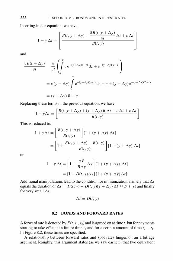
222 FIXED INCOME, BONDS AND INTEREST RATES
Inserting in our equation, we have:
1 + y t =
B(t, y + y) + ∂ B(t, y + y)
∂tt + c t
B(t, y)
and
∂ B(t + y)
∂t= ∂
∂t
T∫
t
c e−(y+y)(z−t) dz + e−(y+y)(T −t)
= c (y + y)
T∫
t
e−(y+y)(z−t) dz − c + (y + y) e−(y+y)(T −t)
= (y + y) B − c
Replacing these terms in the previous equation, we have:
1 + yt =[
B(t, y + y) + (y + y) B t − c t + c t
B(t, y)
]
This is reduced to:
1 + yt =[
B(t, y + y)
B(t, y)
][1 + (y + y) t]
=[
1 + B(t, y + y) − B(t, y)
B(t, y)
][1 + (y + y) t]
or
1 + y t =[
1 + B
Byy
][1 + (y + y) t]
= [1 − D(t, y)y] [1 + (y + y) t]
Additional manipulations lead to the condition for immunization, namely that tequals the duration or t = D(t, y) − D(t, y)(y + y) t ≈ D(t, y) and finallyfor very small t
t = D(t, y)
8.2 BONDS AND FORWARD RATES
A forward rate is denoted by F(t, t1, t2) and is agreed on at time t , but for paymentsstarting to take effect at a future time t1 and for a certain amount of time t2 − t1.In Figure 8.2, these times are specified.
A relationship between forward rates and spot rates hinges on an arbitrageargument. Roughly, this argument states (as we saw earlier), that two equivalent

BONDS AND FORWARD RATES 223
t1 2tt
Figure 8.2
investments (from all points of view) have necessarily the same returns. Say thatat time t we invest $1 for a given amount of time t2 − t at the available spotrate (its yield). The price of such an investment using a bond is then: B(t, t2).Alternatively, we could invest $1 for a certain amount of time, say t1 − t, t1 ≤ t2at which time the moneys available will be reinvested at a forward rate for theremaining time interval: t2 − t1. The price of such an investment will then beB(t, t1)B f (t1, t2) where B f (t1, t2) = [1 + F(t, t1, t2)]−(t2−t1) is the value of thebond at time t1 paying $1 at time t2 using the agreed-on (at time t) forwardrate F(t, t1, t2). Since both payments result in $1 both received at time t2 theyhave the same value, for otherwise there will be an opportunity for arbitrage. Forthis reason, assuming no arbitrage, the following relationship must hold (and seeFigure 8.3):
B(t, t2) = B(t, t1)B f (t1, t2) implying B f (t1, t2) = B(t, t2)
B(t, t1)
In discrete and continuous time, assuming no arbitrage, this leads to the followingforward rates:
[1 + F(t, t1, t2)]t2−t1 = [1 + y(t, t2)]t2−t
[1 + y(t, t1)]t1−t (discrete time)
F(t, t1, t2) = y(t, t2)(t2 − t) − y(t, t1)(t1 − t)
(t2 − t1)(continuous time)
In practice, arbitrageurs can make money by using inconsistent valuations by bondand forward rate prices. For complete markets (where no arbitrage is possible),the spot rate (yield) contains all the information regarding the forward marketrate and, vice versa, the forward market contains all the information regardingthe spot market rate, and thus it will not be possible to derive arbitrage profits.In practice, however, some pricing differences may be observed, as stated above,opening up arbitrage opportunities.
t1 2tt
2( , )B t t
1( , )B t t 1 2( , )fB t t
Figure 8.3

224 FIXED INCOME, BONDS AND INTEREST RATES
ProblemAn annuity pays the holder a scheduled payment over a given amount of time(finite or infinite). Determine the value of such an annuity using bond values atthe current time. What would this value be in two years using the current observedrates?
ProblemWhat will be the value of an annuity that starts in T years and will be paidfor M years afterwards? How would you write this annuity it is terminated atthe time the annuity holder passes away (assuming that all payments are thenstopped)?
ProblemSay that we have an obligation whose nominal value is $1000 at the fixed rateof 10 % with a maturity of 3 years, reimbursed in fine. In other words, the firmobtains a capital of $1000 whose cost is 10 %. What is the financial value of theobligation? Now, assume that just after the obligation is issued the interest ratefalls from 10 to 8 %. The firm’s cost of finance could have been smaller. Whatis the value of the obligation (after the change in interest rates) and what is the‘loss’ to the firm.
8.3 DEFAULT BONDS AND RISKY DEBT
Bonds are rated to qualify their standard risks. Standard and Poors, Moody’s andother rating agencies use for example, AAA, AA, A, BB, etc. to rate bonds asmore or less risky. We shall see in section 8.4 that these rating agencies alsoprovide Markov chains, expressing the probabilities that rated firms switch fromone rating to another, periodically adapted to reflect market environment and theconditions particularly affecting the rated firm (for example, the rise and fall ofthe technology sector, war and peace, and their likes).
Consider a portfolio of B-rated bonds yielding 14 %; typically, these are bondswhich currently are paying their coupons, but have a high likelihood of defaultingor have done so in the recent past. A Treasury bond of similar duration yields5.5 %. Thus, in this example, the Junk–Treasury Spread (JTS) is 8.5 %. Now, letus take a look at the spread’s history over the past 13 years (Jay Diamond, Grant’sInterest Rate Observer data).
The spread depicted in Figure 8.4 corresponds roughly to a B-rated debt. Notethe very wide range of spreads, from just below 3 % to almost 10 %. What doesa JTS of 3 % mean? Very bad news for the junk buyer, because he or she willhave been better off in Treasuries if the loss rate exceeds 3 %. And even if theloss rate is only half of that, a 1.5 % return premium does not seem adequate tocompensate for this risk. There is a wealth of data on the bankruptcy/default rate,allowing us to evaluate whether the prevailing risk premium amounts to adequatecompensation.

DEFAULT BONDS AND RISKY DEBT 225
Figure 8.4 Junk–Treasury spread 1988–2000 (Jay Diamond, Grant’s Interest RateObserver data).
Rating agencies often use terms such as default rate and loss rate which areimportant to understand. The former defines the proportion of companies default-ing per year. But not all companies that default go bankrupt. The recovery rateis the proportion of defaulting companies that do not eventually go bankrupt. Soa portfolio’s reduction in return is calculated as the default rate times one minusthe recovery rate: if the default rate is 4 % and the recovery rate is 40 %, thenthe portfolio’s total return has been reduced by 2.4 %. The loss rate, how muchof the portfolio actually disappears, is simply the default rate minus the abso-lute percentage of companies which recover. According to Moody’s, the annuallong-term default rate of bonds rated BBB/Baa (the lowest ‘investment grade’) isabout 0.3 %; for BB/Ba, about 1.5 %; and for B, about 7 %. But in any given year,the default rate varies widely. Further, because of the changes in the high-yieldmarket that occurred 15 years ago, the pre-1985 experience may not be of greatrelevance to high-yield investing today.
Prior to the use of junk bonds the overwhelming majority of speculative issueswere ‘fallen angels’, former investment-grade debt which had fallen on hard times.But, after 1985, most high-yield securities were speculative right from their initialoffering. Once relegated to bank loans, poorly rated companies were for the firsttime able to issue debt themselves. This was not a change for the better. Similarto speculative stock IPOs, these new high-yield bond issues tended to have lesssecure ‘coverage’ (based on an accounting term defined as the ratio of earnings-before-taxes-and-interest to total interest charges) than the fallen angels of yore,and their default rates were correspondingly higher.

226 FIXED INCOME, BONDS AND INTEREST RATES
Many financial institutions hold large amounts of default-prone risky bondsand securities of various degrees of complexity in their portfolios that require areliable estimate of the credit exposure associated with these holdings. Models ofdefault-prone bonds fall into one of two categories: structural models and reduced-form models. Structural models specify that default occurs when the firm valuefalls below some explicit threshold (for example, when the debt to equity ratiocrosses a given threshold). In this sense, default is a ‘stopping time’ defined by theevolution of a representative stochastic process. Merton (1974) first consideredsuch a problem; it was studied further by many researchers including Black andCox (1976), Leland (1994), and Longstaff and Schwartz (1995). These modelsdetermine both equity and debt prices in a self-consistent manner via arbitrage,or contingent-claims pricing. Equity is assumed to possess characteristics similarto a call option, while debt claims have features analogous to claims on the firm’svalue. This interpretation is useful for predicting the determinants of credit-spreadchanges, for example.
Some models assume as well that debt-holders get back a fraction of the debt,called the recovery ratio. This ratio is mostly specified a priori, however. While thisis quite unrealistic, such an assumption removes problems associated to the debtseniority structure, which is a drawback of Merton’s (1974) model. Some authors,for example, Longstaff and Schwartz (1995), argue that, by looking at the historyof defaults and recovery ratios for various classes of debt of comparable firms, onecan find a reliable estimate of the recovery ratio. Structural models are, however,difficult to use in valuing default-prone debt, due to difficulties associated withdetermining the parameters of the firm’s value process needed to value bonds.But one may argue that parameters could always be retrieved from market pricesof the firm’s traded bonds. Further, they cannot incorporate credit-rating changesthat occur frequently for default-prone (risky) corporate debts.
Many corporate bonds undergo credit downgrades by credit-rating agenciesbefore they actually default, and bond prices react to these changes (often brutally)either in anticipation or when they occur. Thus, any valuation model shouldtake into account the uncertainty associated with credit-rating changes as well asthe uncertainty surrounding default and the market’s reactions to such changes.These shortcomings make it necessary to look at other models for the valuation ofdefaultable bonds and securities that are not predicated on the value of the firm andthat take into account credit-rating changes. For example, a meltdown of financialmarkets, wars, political events of economic importance are such cases, where therisk is exogenous (rather than endogenous). This leads to reduced-form models.
The problem of rating the credit of bonds and credit markets is in fact moredifficult than presumed by analytical models. Information asymmetries compoundthese difficulties. Akerlof in his 2001 Nobel allocution pointed to these effectsfurther.
A bank granting a credit has less information than the borrower, on his actual default risk. . . . Onthe same token, banks expanding into new, unknown markets are at a particular risk. On theone hand, due to their imperfect market knowledge, they must rely on the equilibrium betweensupply and demand to a large extent. On the other hand, under asymmetric information, it is very

DEFAULT BONDS AND RISKY DEBT 227
Value
Time
Default level
Figure 8.5 Structural models of default.
easy for clients to hide risks and to give too optimistic profit estimates, possibly approachingfraud in extreme cases. Adverse selection then implies a markedly increased default risk forsuch banks. Banks can use interest rates and additional security as instruments for screeningthe creditworthiness of clients when they estimate that their information is insufficient. Creditrisk and pricing models, of course, are complementary tools. Based on information providedby the client, they produce risk-adjusted credit spreads and thus may set limits to the principleof supply and demand. On the other hand, borrowers with a credit rating may use this rating tosignal the otherwise private information on their solvency, to the bank. In exchange, they expectto receive better credit conditions than they would if the bank could only use information onsample averages.
Technically, the value process is defined in terms of a stochastic process x, t ≥ 0while default is defined by the first time τ (the stopping time) the process reachesa predefined threshold-default level. In other words, let the threshold space be ,then:
τ = Inf t > 0, x(t) /∈ where is used to specify the set of feasible states for an operating firm. As soonas the firm’s value is out of these states, default occurs.
Reduced-form models specify the default process explicitly, interpreting it asan exogenously motivated jump process, usually expressed as a function of thefirm value. This class of models has been investigated, for example by Jarrowand Turnbull (1995), Jarrow et al. (1997) and others. Although these modelsare useful for fitting default to observed credit spreads, they mostly neglect theunderlying value process of the firm and thus they can be less useful when it isnecessary to determine credit spread variations. Jarrow et al. (1997) in particularhave adopted the rating matrix used by financial institutions such as Moody’s,Standard and Poors and others as a model of credit rating (as we too shall do inthe next section).
Technically, default is defined exogenously by a random variable T wheret < T < T , with T , the bond expiry date. The conditional probability of defaultis assumed given by:
P(T ∈ (t + dt)∣∣t < T < T ) = q(x) dt + 0(dt)

228 FIXED INCOME, BONDS AND INTEREST RATES
Value
Time
Default levelJump timeto default
Figure 8.6 Reduced-form models default.
This means that the conditional probability of default q in a small time interval (t +dt), given that no default has occurred previously, is a function of an underlyingstochastic process x, t ≥ 0. If the probability q is independent of the processx, t ≥ 0, this implies that the probability of default is of the exponential type.That is to say, it implies that at each instant of time, the probability of defaultis time-independent and independent of the underlying economic fundamentals.These are very strong assumptions and therefore, in practice, one should be verycareful in using these models.
A comparison between structural and reduced-form models (see Figure 8.6) isoutlined in Table 8.2. Selecting one model or the other is limited by the underlyingrisk considered and the mathematical and statistical tractability in applying sucha model. These problems are extensively studied, as the references at the end ofthe chapter indicate.
A general technical formulation, combining both structural and reduced-formmodels leads to a time to default we can write by Min(τ, T , T ) where T is thematurity reached if no default occurs, while exogenous and endogenous defaultare given by the random variables (τ, T ). If the yield of such bonds at time t for apayout at s is given by, Y (t, s) ≡ y(τ, T , s), the value of a pure default-prone bondpaying $1 at redemption is then E exp(−Y (t, T ) Min(τ, T , T )). Of course if therewas no default, the yield would be y(t, s) and therefore Y (t, s) > y(t, s) in orderto compensate for the default risk. The essential difficulty of these problemsis to determine the appropriate yield which accounts for such risks, however.For example, consider the current value of a bond retired at Min(τ, T , T ) andpaying an indexed coupon payout indexed to some economic variable or economicindex (inflation, interest rate etc.). Uncertainty regarding the coupon payment, itsnominal value and the bond default must then be appropriately valued throughthe bond yield.
When a bond is freely traded, the coupon payment can also be interpreted asa ‘bribe’ paid to maintain bond holding. For example, when a firm has couponpayments that are too large, it might redeem the bond (provided it incurs the costsassociated with such redemption). By the same token, given an investor withother opportunities, deemed better than holding bonds, it might lead the investorto forgo future payouts and principal redemption, and sell the bond at its current

DEFAULT BONDS AND RISKY DEBT 229
Table 8.2 A comparison of selected models.
Model Advantages Drawbacks
Merton(1974)
Simple to implement. (a) Requires inputs about the firmvalue.
(b) Default occurs only at debtmaturity.
(c) Information about default andcredit-rating changes cannot beused.
Longstaffand Schwartz(1995)
(a) Simple to implement.(b) Allows for stochastic term
structure and correlation betweendefaults and interest rates.
(a) Requires inputs related to thefirm value.
(b) Information in the history ofdefaults and credit-ratingchanges cannot be used.
Jarrow, Lando,and Turnbull(1997)
(a) Simple to implement.(b) Can match exactly existing prices
of default-risky bonds and thusinfer risk-neutral probabilities fordefault and credit-rating changes.
(c) Uses the history of default andcredit-rating change.
(a) Correlation not allowed betweendefault probabilities and thelevel of interest rates.
(b) Credit spreads change onlywhen credit ratings change.
Lando(1998)
(a) Allows correlation between defaultprobabilities and interest rates.
(b) Allows many existingterm-structure models to be easilyembedded in the valuationframework.
Historical probabilities of defaultsand credit-rating changes are usedassuming that the risk premiums dueto defaults and rating changes, isnull.
Duffie andSingleton(1997)
(a) Allows correlation between defaultprobabilities and the level ofinterest rates.
(b) Recovery ratio can be random anddepend on the pre-default value ofthe security.
(c) Any default-free term-structuremodel can be accommodated, andexisting valuation results fordefault-free term-structure modelscan be readily used.
Information regarding credit-ratinghistory and defaults cannot be used.
Duffie andHuang(1996) (swaps)
(a) Has all the advantages of Duffieand Singleton.
(b) Asymmetry in credit qualities iseasily accommodated.
(c) ISDA guidelines for settlementupon swap default can beincorporated.
(a) Information regardingcredit-rating history and defaultscannot be used.
(b) Computationally difficult toimplement for some swaps, suchas cross-currency swaps, ifdomestic and foreign interestrates are assumed to be random.
230 FIXED INCOME, BONDS AND INTEREST RATES
market value. The number of cases we might consider is very large indeed, butonly a few such cases will be considered explicitly here.
Structural and reduced-form models for valuing default-prone debt do not in-corporate financial restructuring (and potential recovery) that often follows de-fault. Actions such as renegotiating the terms of a debt by extending the maturityor lowering/postponing promised payments, exchanging debt for other forms ofsecurity, or some combination of the above (often being the case after default),are not considered. Similarly, institutional and reorganization features (such asbankruptcy) cannot be incorporated in any of these models simply. Further, an-ticipated debt restructurings by the market is priced in the value of a defaultablebond in ways that none of these models captures. In fact, many default-prone se-curities are also thinly traded. Thus, a liquidity premium is usually incorporatedinto these bond prices, hiding their risk of default. Finally, empirical evidence forthese models is rather thin. Duffie and Singleton (1997, 1999) find that reduced-form models have problems explaining the observed term structure of creditspreads across firms of different credit qualities. Such problems could arise fromincorrect statistical specifications of default probabilities and interest rates orfrom models’ inability to incorporate some of the features of default/bankruptcymentioned above. Bond research, just like finance in general, remains thereforea domain of study with many avenues to explore and questions that are still farfrom resolved.
8.4 RATED BONDS AND DEFAULT
The potential default of bonds and changes in rating are common and outstandingissues to price and reckon with in bonds trading and investment. They can occurfor a number of reasons, including some of the following:
(1) Default of the payout or default on the redemption of the principal.(2) Purchasing power risk arising because inflationary forces can alter the value
of the bond. For example, a bond which is not indexed to a cost of livingindex may in fact generate a loss to the borrower in favour of the lendershould inflation be lower than anticipated thereby increasing the real orinflation-deflated payments.
(3) Interest-rate risk, resulting from predictable and unpredictable variations inmarket interest rates and therefore the bond yield.
(4) Delayed payment risk, and many other situations associated with the finan-cial health of the bond issuer and its credit reliability.
These situations are difficult to analyse but rating agencies specializing in the anal-ysis and the valuation of financial assets provide ratings to nations and corporateentities that are used to price bonds. These agencies provide explicit matricesthat associate to various bond classes (AAA, AA, B etc.) probabilities (a Markovchain) of remaining in a given class or switching to another (higher or lower) risk(rating) class. Table 8.3 shows a scale of ratings assigned to bonds by financial

RATED BONDS AND DEFAULT 231
Table 8.3 Ratings.
Moody’s S&P Definition
Aaa AAA Highest rating availableAa AA Very high qualityA A High qualityBaa BBB Minimum investment gradeBa BB Low gradeB B Very speculativeCaa CCC Substantial riskCa CC Very poor qualityC D Imminent default or in default
firms services (Moody’s, Standard and Poors etc.) that start from the best qual-ity to the lowest. In addition to these ratings, Moody’s adds a ‘1’ to indicate aslightly higher credit quality; for instance, a rating of ‘A1’ is slightly higher thana rating of ‘A’ whereas ‘A3’ is slightly lower. S&P ratings may be modified by theaddition of a ‘+’ or ‘−’ (plus or minus). ‘A+’ is a slightly higher grade than ‘A’and ‘A−’ is slightly lower. Occasionally one may see some bonds with an ‘NR’in either Moody’s or S&P. This means ‘not rated’; it does not necessarily meanthat the bonds are of low quality. It basically means that the issuer did not applyto either Moody’s or S&P for a rating. Government agencies are a good exampleof very high quality bonds that are not rated by S&P. Other things being equal,the lower the rating, the higher the yield one can expect. Insured bonds have thehighest degree of safety of all non-government bonds. Bond insurance agenciesguarantee the payment of principal and interest on the bonds they have insured(since insurance reduces the bond’s risk). When bonds are insured by one of themajor insurance agencies, they automatically attain ‘AAA’ rating, identifying thebond as one of the highest quality one can buy. Some of the major bond insurersare AMBAC, MBIA, FGIC and FSA. In such circumstances, bonds have almostno default risk.
The Moody’s rating matrix shown in Table 8.4 is an example. For AAA bonds,the probability that it maintains such a rating is .9193 while there is a .0746probability that the bond rating is downgraded to a AA bond and so on forremaining values. These matrices are updated and changed from time to time asbusiness conditions change. Given these matrices we observe that even a tripleAAA bond is ‘risky’ since there is a probability that it be downgraded and itsprice reduced to reflect such added risk.
In some cases, the price of downgrading the credit rating of a firm can be muchlarger than presumed. For example, buried in Dynegy Inc.’s. annual report for2001 is a ‘$301 million paragraph’. The provision is listed on page 28 of a 114-page document is the only published disclosure showing that Dynegy will haveto post that much collateral if the ratings of its Dynegy Holdings Inc. unit are cutto junk status, or below investment grade. Debtors like Dynegy, WorldCom Inc.and Vivendi Universal SA are obligated to pay back billions of dollars if their

232 FIXED INCOME, BONDS AND INTEREST RATES
Table 8.4 A typical Moody’s rating matrix.
AAA AA A BBB BB B CCC D NR
AAA 91.93 % 7.46 % 0.48 % 0.08 % 0.04 % 0.00 % 0.00 % 0.00 % —
AA 0.64 % 91.81 % 6.76 % 0.60 % 0.06 % 0.12 % 0.03 % 0.00 % —
A 0.07 % 2.27 % 91.69 % 5.12 % 0.56 % 0.25 % 0.01 % 0.04 % —
BBB 0.04 % 0.27 % 5.56 % 87.88 % 4.83 % 1.02 % 0.17 % 0.24 % —
BB 0.04 % 0.10 % 0.61 % 7.75 % 81.48 % 7.90 % 1.11 % 1.01 % —
B 0.00 % 0.10 % 0.28 % 0.46 % 6.95 % 82.80 % 3.96 % 5.45 % —
CCC 0.19 % 0.00 % 0.37 % 0.75 % 2.43 % 12.13 % 60.45 % 23.69 % —
D 0.00 % 0.00 % 0.00 % 0.00 % 0.00 % 0.00 % 0.00 % 100.00 % —
credit ratings fall, their stock drops or they fail to meet financial targets. Half ofthese so-called triggers have not been disclosed publicly, according to Moody’sInvestors Service Inc., which has been investigating the presence of such clausessince the collapse of the Enron Corp. (International Herald Tribune, May 9 May2002, p. 15). In other words, in addition to a corporation’s rating, there are othersources of information, some revealed and some hidden, that differentiate thevalue of debt for such corporations, even if they are equally rated. In other words,their yield may not be the same even if they are equally rated. The rating of bondsis thus problematic, although there is an extensive insurance market for bondsthat index premiums to the bond rating. A dealer’s quotes in Moody’s provides,for example, an estimate of insurance costs for certain bonds (determined by theswap market), some of which are reproduced in Table 8.5. The premium paidvaries widely, however, based on both the rating and the perceived viability of thecompany whose bond is insured.
Table 8.5 Date-Moody’s, 20 May 2002.
Premium cost per Moody’s SeniorCompany $M for 5 years Debt Rating
Merrill Lynch 10 000 Aa3Lehman Brothers 9 500 A2American Express 8 000 A1Bear Stearns 7 500 A2Goldman Sachs 6 500 A1GE Capital 6 500 AaaMorgan Stanley 6 500 Aa3JP Morgan Chase 6 500 Aa3*AIG 5 300 AaaCitigroup 4 000 Aa1*Bank of America 4 000 Aa2*Bank One 3 500 Aaa

RATED BONDS AND DEFAULT 233
The valuation of rated bonds is treated next by making some simplifying as-sumptions to maintain an analytical and computational tractability, and by solvingsome problems that highlight approaches to valuing rated bonds. Rating can onlyserve as a first indicator to future default risk. Good accounting, information(statistical and otherwise) and economic analyses are still necessary.
8.4.1 A Markov chain and rating
Consider first a universe of artificial (and in fact non-existing) coupon-bearingrated bonds with a payment of a dollar fraction i at maturity T , depending onthe rating of the bond at maturity. Risk is thus induced only by the fraction 1 − i
lost at maturity. Further, define the bond m-ratings matrix by a Markov chain [pij]where
0 ≤ pij ≤ 1,
m∑
j=1
pij = 1
denotes the objective transition probability that a bond rated i in a given periodwill be rated j in the following one. Discount factors are a function of the ratingstates, thus a bond rated i has a spot (one period) yield Rit , Rit ≤ R jt for i < jat time t . As a result, a bond rated i at time t and paying a coupon cit at this timehas, under the usual conditions, a value given by:
Bi,t = cit +m∑
j=1
pij
1 + R jtB j,t+1; Bi,T = i , i = 1, 2, 3, . . . , m
Note that the discount rate R jt is applied to a bond rated j in the next period.For example, for an ‘imaginary’ rated bond A and D only, each with (short-term) yields (RAt , RDt ) at time t and a rating matrix specified by the transitionprobabilities, [pij]; i, j = A, D, we have:
BA,t = cA,t +[
pAA
1 + RAtBA,t+1 + pAD
1 + RDtBD,t+1
]; BA,T = A = 1
BD,t = cD,t +[
pDA
1 + RAtBA,t+1 + pDD
1 + RDtBD,t+1
]; BD,T = D
where (cA,t , cD,t ) are the payouts associated with the bond rating and (A, D)are the bond redemption values at maturity T , both a function of the bond rating.In other words, the current value of a rated bond equals current payout plus theexpected discount value of the bond rated at all classes, using the correspondingyield for each class at time t + 1. Of course, at the terminal time, when the bondis due (since there is not yet any default), the bond value equals its nominal value.If at maturity the bond is rated A, it will pay the nominal value of one dollar(A = 1) while if it is rated D, it will imply a loss of 1 − D for a bond ratedinitially A. If we define D as a default state (i.e. where the bondholder cannotrecuperate the bond nominal value), the D can be interpreted as the recuperationratio. Of course, we can assume as well D = 0 as will be the case in a number

234 FIXED INCOME, BONDS AND INTEREST RATES
of examples below. In vector notation we have:
[BA,t
BD,t
]=
[cA,t
cD,t
]+
pAA
1 + RAt
pAD
1 + RDt
pDA
1 + RAt
pDD
1 + RDt
[BA,t+1
BD,t+1
];
[BA,T
BD,T
]=
[A
D
];
where i is the nominal value of a bond rated i at maturity. And generally, for anm-rated bond,
Bt= ct + Ft Bt+1, BT = L
Note that the matrix Ft has entries [pij/(1 + R jt )] and L is a diagonal matrix ofentries i , i = 1, 2, . . . , m. For a zero-coupon bond, we have:
Bt =T∏
k=t
FkL.
By the same token, rated bonds discounts qit = 1/(1 + Rit ) are found by solvingthe matrix equation:
q1t
q2t
...
...
qmt
=
p11 B1,t+1 p12 B2,t+1 ... ... p1m Bm,t+1
p21 B1,t+1 p22 B2,t+1 p2m Bm,t+1
...
...
pm1 B1,t+1 pm2 B2,t+1 pmm Bm,t+1
−1
B1,t − c1t
B2,t − c2t
...
...
Bm,t − cmt
where at maturity T , Bi,T = i . Thus, in matrix notation, we have:
qt = −1t+1 (Bt−ct )
Note that one period prior to maturity, we have: qT −1 = −1T (BT −1−cT −1) where
T is a matrix with entries pij B j,T = pij j . For example, for the two-ratings bond,we have:
B1,t = c1t + q1t p11 B1,t+1 + q2t p12 B2,t+1; B1,T = 1
B2,t = c2t + q1t p21 B1,t+1 + q2t p22 B2,t+1; B2,T = 2
Equivalently, in matrix notation, this is given by:[
q1t
q2t
]=
[p11 B1,t+1 p12 B2,t+1
p21 B1,t+1 p22 B2,t+1
]−1 [B1,t − c1t
B2,t − c2t
]
In this sense the forward bond price can be calculated by the rated bond discountrate and vice versa.
ExampleWe consider the matrix representing a rated bond supplied by Moody’s (Table 8.6).The discount rates Ri , i = AAA, . . . , D for each class and the correspondingcoupon payments are given in Table 8.7. For example, the discount rate of anAAA bond is 0.06 yearly while that of a BBB bond is 0.1. In addition, the AAA-rated bond has a coupon paying $1, while if it were rated BB its coupon payment

RATED BONDS AND DEFAULT 235
Table 8.6
AAA AA A BBB BB B CCC D
AAA 0.9193 0.0746 0.0048 0.0008 0.0004 0 0 0
AA 0.0064 0.9181 0.0676 0.006 0.0006 0.0012 0.0003 0
A 0.0007 0.0227 0.9169 0.0512 0.0056 0.0025 0.0001 0.0004
BBB 0.0004 0.0027 0.0556 0.8788 0.0483 0.0102 0.0017 0.0024
BB 0.0004 0.001 0.0061 0.0775 0.8148 0.079 0.0111 0.0101
B 0 0.001 0.0028 0.0046 0.0695 0.828 0.0396 0.0545
CCC 0.0019 0 0.0037 0.0075 0.0243 0.1213 0.6045 0.2369
D 0 0 0 0 0 0 0 1
would have to be $1.4. In this sense, both the size of the coupon and the discountapplied to the rated bond are used to pay for the risk associated with the bond. Thebond nominal value is $100 with a lifetime of ten years. An elementary programwill yield then the following bond value, shown above for each class at each yeartill the bond’s redemption. For example, initially, the premium paid for a AAAbond compared to a AA one is (63.10−58.81) = $4.29. At the end of the fifthyear, however, the AAA–AA bond price differential is only 82.59–80.11 = $2.48.In fact, we note that the smaller the amount of time left to bond redemption, thesmaller the premium.
8.4.2 Bond sensitivity to rates – Duration
For the artificial rated bond considered above, we can calculate the durationof a rated bond through the rated bond sensitivity to the yields of each rating.For simplicity, assume that short yields are constants and calculate the partialderivatives for a bond rated A or D only. In this case, we seek to calculate thepartials:
[∂ BA,t
∂ RA,∂ BA,t
∂ RD,∂ BD,t
∂ RA,∂ BD,t
∂ RD
],
∂ BA,t
∂ RA= − pAA
(1 + RA)2 BA,t+1+ pAA
1 + RA
∂ BA,t+1
∂ RA+ pAD
1 + RD
∂ BD,t+1
∂ RA;∂ BA,T
∂ RA= 0
∂ BA,t
∂ RD=
[pAA
1 + RA
∂ BA,t+1
∂ RD− pAD
(1 + RD)2 BD,t+1+ pAD
1 + RD
∂ BD,t+1
∂ RD
];∂ BA,T
∂ RD= 0
∂ BD,t
∂ RA=
[− pDA
(1 + RA)2 BA,t+1 + pDA
1 + RA
∂ BA,t+1
∂ RA+ pDD
1 + RD
∂ BD,t+1
∂ RA
];∂ BD,T
∂ RA= 0
∂ BD,t
∂ RD=
[pDA
1 + RA
∂ BA,t+1
∂ RD− pDD
(1 + RD)2 BD,t+1 + pDD
1 + RD
∂ BD,t+1
∂ RD
];∂ BD,T
∂ RD= 0

Tabl
e8.
7
AA
A1
AA
1.1
A1.
2
BB
B1.
3
BB
1.4
B1.
5
CC
C1.
6
D1.
7
AA
A0.
06
AA
0.07
A0.
08
BB
B0.
09
BB
0.1
B0.
11
CC
C0.
12
D0.
13
Res
ults
AA
AA
AA
BB
BB
BB
CC
CD
T=0
63.1
058
.81
54.8
551
.30
47.8
944
.84
42.3
239
.88
T=1
65.8
961
.78
57.9
654
.50
51.1
548
.13
45.6
143
.15
T=2
68.8
464
.96
61.3
258
.00
54.7
451
.78
49.2
946
.83
T=3
71.9
868
.37
64.9
561
.80
58.7
055
.84
53.4
151
.00
T=4
75.3
172
.02
68.8
865
.95
63.0
460
.34
58.0
355
.71
T=5
78.8
475
.92
73.1
270
.48
67.8
365
.35
63.2
061
.03
T=6
82.5
980
.11
77.7
075
.41
73.1
070
.91
68.9
967
.05
T=7
86.5
684
.58
82.6
480
.79
78.8
977
.08
75.4
873
.84
T=8
90.7
889
.38
87.9
986
.65
85.2
783
.93
82.7
581
.52
T=9
95.2
594
.51
93.7
693
.04
92.2
891
.55
90.8
890
.20
T=1
010
010
010
010
010
010
010
010
0

RATED BONDS AND DEFAULT 237
We can write in vector notation a system of six simultaneous equations given by:
Γt =[
BA,t , BD,t ,∂ BA,t
∂ RA,∂ BA,t
∂ RD,∂ BD,t
∂ RA,∂ BD,t
∂ RD
];
where Γt = Ct + ΦΓt+1,ΓT = [A, D, 0, 0, 0, 0] ; Ct = [cA, cD, 0, 0, 0, 0]
Φ =
pAA
1 + RA
pAD
1 + RD0 0 0 0
pDA
1 + RA
pDD
1 + RD0 0 0 0
− pAA
(1 + RA)2 0pAA
1 + RA0
pAD
1 + RD0
0 − pAD
(1 + RD)2 0pAA
1 + RA0
pAD
1 + RD
− pDA
(1 + RA)2 0pDA
1 + RA0
pDD
1 + RD0
0 − pDD
(1 + RD)20
pDA
1 + RA0
pDD
1 + RD
A solution to this system of equations is found similarly by backward recursion.Namely, for a time-invariant coupon payout, we have:
ΓT −n =n∑
j=1
[Φ]j−1 C + [Φ]n ΓT L, n = 0, 1, 2, . . .
while for a nonpaying coupon bond, we have:
ΓT −n = [Φ]n ΓT , n = 0, 1, 2, . . .
These equations can be solved numerically providing thereby a combined estimateof rated bond prices and their yield sensitivity.
Generally, we can also calculate rated bonds’ duration and their ‘cross-duration’. Bond duration is now defined in terms of partial durations, expressingthe effects of all yields rates. Explicitly, say that a bond is rated i at time t andfor simplicity let the yields be time-invariant. The duration of a bond rated i withrespect to its yield is denoted by Dii (t, T ), i = 1, 2, . . . , m, with,
Dii (t, T ) = − 1
Bi,t
∂ Bi,t
∂ Ri
while the partial duration, of the bond rated i with respect to any other yield, R j ,i = j is:
Di j (t, T ) = − 1
Bi,t
∂ Bi,t
∂ R j= −∂
(log Bi,t
)
∂ R j; i = j

238 FIXED INCOME, BONDS AND INTEREST RATES
By the same token, for convexity we have:
ϒi i (t, T ) = 1
Bi,t
∂2 Bi,t
∂ R2i
and ϒi j (t, T ) = 1
Bi,t
∂2 Bi,t
∂ Ri∂ R j
The partial durations and convexities express the sensitivity of a bond rated i isthus:
dBi,t
Bi,t= 1
Bi,t
∂ Bi,t
∂tdt + 1
Bi,t
m∑
j=1
∂ Bi,t
∂ R jdR j + 1
2
1
Bi,t
m∑
j=1
∂2 Bi,t
∂ R j∂ RidRi dR j
Or:
dBi,t
Bi,t− ∂ log Bi,t
∂tdt = −
m∑
j=1
Di j dR j + 1
2
m∑
j=1
ϒi j dRi dR j
ExampleConsider a bond with three ratings (1, 2 and 3) and assume constant yields foreach given by (R1, R2, R3) = (0.05; 0.07; 0.10). Let the ratings transition matrixbe:
P =
0.9 0.1 00.05 0.8 0.150.00 0.05 0.95
Then the bond recursive equation for a pure bond paying $1 in two periods is:
Bi,t =m∑
j=1
pij
1 + R jB j,t+1; Bi,2 = i , i = 1, 2, 3, . . . , m, t = 0, 1, 2
For m = 3, this is reduced to:
B1,0 = (0.81q11 + 0.005q12)1 + (0.09q12 + q220.08)2 + 0.015q233
B2,0 = (0.045q11 + 0.04q12)1 + (0.005q12 + 0.64q22 + 0.0075q23) 2
+ (0.12q23 + 0.1425q33) 3
B3,0 = (0.0025q12) 1 + (0.04q22 + 0.0475q23)2 + (0.0075q23 + 0.9025q33)3
with the notation:
qi j = 1
1 + Ri
1
1 + R j
and,
q11 = .9068, q12 = 0.8899, q13 = 0.8656,
q22 = 0, 8732, q23 = 0.8494, q33 = 0.8262

RATED BONDS AND DEFAULT 239
Thus,
B1,0 = 0.73891 + 0.097 882 + 0.01273
B2,0 = 0.07631 + 0.56952 + 0.21963
B3,0 = 0.002 221 + 0.07522 + 0.74563
Therefore, a bond rated ‘1’ is worth more than a bond rated ‘2’ and a ‘2’ isworth more than a ‘3’ if B1,0 > B2,0 > B3,0. Their difference accounts for theyield differential associated with each bond rating. Of course, if the rated bondis secured throughout the two periods (i.e. it does not switch from class to class),we have:
B1,0 = 1
(1 + R1)2= 0.907; B2,0 = 1
(1 + R2)2= 0.8734;
B3,0 = 1
(1 + R3)2= 0.8264
The difference between these numbers accounts for a premium implied by theratings switching matrix. For the bond rated ‘3’, we note that the secured ‘rate 3’bond is worth less than the rated bond, accounting for the potential gain in yieldif the bond credit quality is improved. Alternatively, we can use the risk-freediscount rate R f = 0.04 assumed for simplicity to equal 4 % yearly (since thebond has no default risk). In this case,
B f,0 = 1
(1 + R f )2= 1
(1 + 0.04)2= 0.9245
The premium for such a risk-free bond compared to a secured bond rated ‘1’, is0.9245 − 0.907l.
8.4.3 Pricing rated bonds and the term structure risk-free rates∗
When the risk-free term structure is available, and assuming no arbitrage, we canconstruct a portfolio replicating the bond, thereby valuing the rated bond yieldsfor each bond class. Explicitly, consider a portfolio of rated bonds consisting ofNi , i = 1, 2, 3, . . . , m bonds rated i , each providing i dollars at maturity. Letthe portfolio value at maturity be equal to $1. That is to say
m∑
i=1
Ni Bi,T =m∑
i=1
Nii = 1
One period (year) prior to maturity, such a portfolio would be worth
m∑
i=1
Ni Bi,T −1

240 FIXED INCOME, BONDS AND INTEREST RATES
dollars. By the same token, if we denote by R f,T −1 the risk-free discount rate forone year, then assuming no arbitrage, one period prior to maturity, we have:
m∑
i=1
Ni Bi,T −1 = 1
1 + R f,T −1; Bi,T −1 = cit +
m∑
j=1
q j,T −1 pij B j,T ;
Bi,T = i , i = 1, 2, . . . , m
with q jt = 1/(1 + R j,t ) and R j,t is the one-period discount rate applied to aj-rated bond. This system of equations provides 2m unknown rates and the port-folio composition with only one equation is therefore under-determined. For twoperiods we have an additional equation:
m∑
i=1
Ni Bi,T −2 = 1
(1 + R f,T −1)2
While the bond price is given by:
Bi,T −2 = ci,T −2 +m∑
j=1
q j,T −2 pij B j,T −1; Bi,T = i , i = 1, 2, . . . , m
as well as:
Bi,T −2 = ci,T −2 +m∑
j=1
q j,T −2,2 p(2)ij B j,T ; Bi,T = i , i = 1, 2, . . . , m
where p(2)ij is the probability that the bond is rated j two periods hence while
q j,T −2,2 is the discount rate for a j-rated bond for two periods forward (that mightdiffer from the rate q j,T −2,1 applied for one period only). Here again, we see thatthere are 2m rates while there are only two equations. For three periods we willhave three equations per rating and so on. Generally, k periods prior to maturity,assuming no arbitrage, we have the following conditions for no arbitrage:
m∑
i=1
Ni Bi,T −k = 1
(1 + R f,T −k)kk = 0, 12, 3, . . . , T
Bi,T −k = ci,T −k +m∑
j=1
q j,T −k,h p(h)ij B j,T −(k−h); Bi,T = i ,
i = 1, 2, . . . , m; k = 1, 2, 3, . . . , T ; h = 1, 2, 3, . . . , k
where R f,T −k, k = 1, 2, 3, . . . , is the risk-free rate term structure and p(h)ij is
the ij entry of the h-power of the rating matrix. These provide a system of T + 1simultaneous equations spanning the bond life. In matrix notation this is given by:
NBT −k = 1
(1 + R f,T −k)kk = 0, 1, 2, . . . , T ; N = (N1, . . . , Nm) ;
BT −k = (B1,T −k, . . . , Bm,T −k)

RATED BONDS AND DEFAULT 241
as well as:
Bt−k = ct−k + F(h)t Bt+(k−h); BT = L,
F(h)t =
[q j,T −k,h p(h)
ij
]; h = 1, 2, . . . , k; k = 1, 2, . . . , T
This renders the estimation of the term structure of ratings discount grosslyunder-determined. However, some approximations can be made which may beacceptable practically. Such an approximation consists in assuming that the ratesat a given time are assumed time-invariant and the term structure of risk-freerates is known and we only estimate the short ratings discount. We assume firstthe case of a maturity larger than the number of rating classes.
Case T ≥ 2mWhen the bond maturity is larger than the number of ratings T ≥ 2m, andq j,T −k,h = q j,h, h = 1 and q j,1 = q j , the hedging portfolio of rated bonds isfound by a solution of the system of linear equations above (with h = 1), leadingto the unique solution:
N∗ = −1Ω
where is the matrix transpose of [Bi,T − j+1] and Ω is a column vector withentries [1/(1 + R f,T −s)s], s = 0, 1, 2, . . . , m − 1. Explicitly, we have:
N1
N2
...
...
Nm
=
B1,T B2,T B3,T ... Bm,T
B1,T −1 B2,T −1 B3,T −1 ... Bm,T −1
... ...
... ...
B1,T −m B2,T −m B3,T −m ... Bm,T −m
−1
11/(1 + R f,T −1)1
...
...
1/(1 + R f,T −m)m
Thus, the condition for no arbitrage is reduced to satisfying a system of systemof nonlinear equations:
−1ΩBT −k = 1
(1 + R f,T −k)k; k = m, m + 1, . . . , T
For example, for a zero-coupon rated bond and stationary short discounts, wehave Bt−k = (F)k L and therefore, the no-arbitrage condition becomes:
−1Ω (F)k L = 1
(1 + R f,T −k)k; k = m, m + 1, . . . , T
where F has entries q j pij. This provides, therefore, T + 1 − m equations appliedto determining the bond ratings short (one period) discount rates q j .
Our system of equations may be over- or under-identified for determiningthe ratings discount rates under our no-arbitrage condition. Of course, if T +1 − m = m, we have exactly m additional equations we can use to solve theratings discount rates uniquely (albeit, these are nonlinear equations and can besolved only numerically). If (T ≥ 2m + 1) we can use the remaining equationsto calculate some of the term structure discounts of bond ratings as well. For

242 FIXED INCOME, BONDS AND INTEREST RATES
example, for a bond with maturity three times the number of ratings, T = 3m,we have the following no-arbitrage condition:
−1ΩBT −k = 1
(1 + R f,T −k)k; k = m, m + 1, . . . , T
and
Bi,T −k = ci,T −k +m∑
j=1
q j,1 p(1)ij B j,T −(k−1); Bi,T = i ,
Bi,T −k = ci,T −k +m∑
j=1
q j,2 p(2)ij B j,T −(k−2); Bi,T = i ,
i = 1, 2, . . . , m; k = 1, 2, 3, . . . , T
Thus, when the bond maturity is very large (or if we consider a continuous-timebond), an infinite number of equations is generated which justifies the conditionfor no arbitrage stated by Jarrow et al. (1997).
When data regarding the risk-free term structure is limited, or for short bonds,we have, m ≤ T < 2m and the Markov model is incomplete. We must, therefore,proceed to an approach that can, nevertheless, provide an estimate of the ratingsdiscount rates. We use for convenience a sum of squared deviations from the ratedbond arbitrage condition, in which case we minimize the following expression(for estimating the short discount rates only):
Minimize0 ≤ q1,q2,....qm−1,qm ≤ 1
T∑
k=m
(−1ΩBT −k − 1
(1 + R f,T −k)k
)2
subject to a number of equalities used in selecting the portfolio, namely:
Bi,T −k = ci,T −k +m∑
j=1
q j,1 p(1)ij B j,T −(k−1); Bi,T = i , k = 1, 2, . . . , T
Additional constraints, reflecting expected and economic rationales of the ratingsdiscounts q j might be added, such as:
0 ≤ q j ≤ 1 as well as 0 ≤ qm ≤ qm−1 ≤ qm−2 ≤ qm−3, . . . ,≤ q2 ≤ q1 ≤ 1
These are typically nonlinear optimization problems, however. A simple two-ratings problem and other examples are considered to highlight the complexitiesin determining both the hedging portfolio and the ratings discounts provided therisk-free term structure is available.
Example: Valuation of a two-rates rated bondFor a portfolio of two-rates bonds over one period where 1 = 1, 2 = 0.2 wehave the following two equations that can be used to calculate the risk-free

RATED BONDS AND DEFAULT 243
portfolio composition:
N1 + 0.2N2 = 1 or N2 = 5(1 − N1)
N1 B1,T −1 + 5(1 − N1)B2,T −1 = 1
1 + R f,T −1
and,
N1 = B2,T −1(1 + R f,T −1) − 0.2
(1 + R f,T −1)(B2,T −1 − 0.2B1,T −1)
If we assume a bond of maturity of three periods only, then only two additionalequations are available (T − 2, T − 3) providing a no-arbitrage estimate for therated bond discounts and given by:
(B2,T −1(1 + R f,T −1) − 0.2
(1 + R f,T −1)(B2,T −1 − 0.2B1,T −1)
)
× (B1,T −2 − 5B2,T −2) + 5B2,T −2 = 1
(1 + R f,T −2)2
(B2,T −1(1 + R f,T −1) − 0.2
(1 + R f,T −1)(B2,T −1 − 0.2B1,T −1)
)
× (B1,T −3 − 5B2,T −3) + 5B2,T −3 = 1
(1 + R f,T −3)3
B1,T −1 = c1,T −1 + q1 p11 + 0.2q2 p12;
B2,T −1 = c2,T −1 + q1 p21 + q2 p220.2
B1,T −2 = c1,T −2 + q1 p11 B1,T −1 + q2 p12 B2,T −1;
B2,T −2 = c2,T −2 + q1 p21 B1,T −1 + q2 p22 B2,T −1
B1,T −3 = [c1,T −3 + q1 p11c1,T −2 + q2 p12c2,T −2]
+ [q21 p2
11 + q1q2 p12 p21]B1,T −1 + [q2q1 p11 p12 + q22 p12 p22]B2,T −1
B2,T −3 = [c2,T −3 + q1 p21c1,T −2 + q2 p22c2,T −2]
+ [q1q1 p21 p11 + q1q2 p12 p21]B1,T −1 + [q2q1 p21 p22 + q22 p2
22]B2,T −1
where, B1,T −1, B1,T −2, B1,T −3 are functions of the bond redemption values andthe ratings discount rates q1 and q2. That is to say, we have a system of twoindependent equations in two unknowns only that we can solve by standardnumerical analysis. For example, consider a zero-coupon bond with a ratingmatrix given by:p11 = 0.8, p12 = 0.2, p21 = 0.1, p22 = 0.9. In addition, set1 = 1, 2 = 0.6 (and therefore a recuperation rate of 60 % on bond default)

244 FIXED INCOME, BONDS AND INTEREST RATES
and R f,T −1 = 0.07, R f,T −2 = 0.08 thus:
B1,T −1 = 0.8q1 + 0.12q2; B2,T −1 = 0.1q1 + 0.54q2
B1,T −2 = 0.8q1 B1,T −1 + 0.2q2 B2,T −1; B2,T −2 = 0.1q1 B1,T −1 + 0.9q2 B2,T −1
B1,T −3 = [0.64q2
1 + 0.02q1q2]
B1,T −1 + [0.16q2q1 + 0.18q2
2
]B2,T −1
B2,T −3 = [0.08q2
1 + 0.02q1q2]
B1,T −1 + [0.09q2q1 + 0.81q2
2
]B2,T −1
and therefore(
1.07B2,T −1 − 0.6
1.07((0.8q1 − 0.6)B1,T −1 + 0.2q2 B2,T −1)
)
× (0.6334q1 B1,T −1 − 1.2294.2q2 B2,T −1)
+ (0.1666q1 B1,T −1 + 1.4994q2 B2,T −1) = 0.8733
(1.07B2,T −1 − 0.6
1.07((0.8q1 − 0.6)B1,T −1 + 0.2q2 B2,T −1)
)
×([
0.5072q21 − 0.013 32q1q2
]B1,T −1+
+ [0.010 06q2q1 − 1.169 46q2
2
]B2,T −1
)
+ ([0.133 28q2
1 + 0.033 32q1q2]
B1,T −1 + [0.14994q2q1 + 1.3446q2
2
]B2,T −1
)
= 0.7937
This is a system of six equations six unknowns that can be solved numerically bythe usual methods.
8.4.4 Valuation of default-prone rated bonds∗
We consider next the more real and practical case consisting in a bonds defaultingprior to maturity and generally we consider the first time n, a bond rated initiallyi , is rated j and let the probability of such an event be denoted by, fij(n). Thisprobability equals the probability of not having gone through a j th rating in priortransitions and be rated j at time n. For transition in one period, this is equal tothe transition bond rating matrix (S&P or Moody’s matrix), while for a transitionin two periods it equals the probability of transition in two periods conditional onnot having reached rating j in the first period. In other words, we have:
fij(1) = pij(1) = pij; fij(2) = pij(2) − fij(1)pjj
By recursion, we can calculate these probabilities:
fij(n) = pij(n) −n−1∑
k=1
fij(k)pjj(n − k)

RATED BONDS AND DEFAULT 245
The probability of a bond defaulting prior to time n is thus,
Fkm(n − 1) =n−1∑
j=1
fkm( j)
while the probability that such a bond does not default is:
Fkm(n − 1) = 1 − Fkm(n − 1)
At present, denote by i (n) the probability that the bond is rated i at time n. Invector notation we write, (n). Thus, given the rating matrix, [P] we have:
(n) = [P]′ (n − 1), n = 1, 2, 3, . . . , and (0) given
with [P]′, the matrix transpose. Thus, at time n, (n) = [P
′]n (0) and the present
value of a coupon payment (given that there was no default at this time) is thereforediscounted at R j,n, q j,n = 1/(1 + R j,n) if the bond is rated j . In other words, itspresent value is:
m−1∑
j=1
c j,nqnj,n j,n; j,n =
m−1∑
i=1
i,0 p(n)ij
where p(n)ij is the ijth entry of the transpose power matrix [P
′]n and i,0 is the
probability that initially the bond is rated i .When a coupon-bearing default bond rated i at time s, defaults at time, s + 1,
T − (s + 1) periods before maturity with probability fim(s + 1 − s) = fim(1), wehave a value:
Vs,i = (ci,T −s + q
m,T −(s+1)
i
)w.p. fim(1)
If such an even occurs at time, s + 2, with probability fim(s + 2 − s) = fim(2),we have:
Vs,i =(
ci,T −s +m−1∑
k=1
qkck,T −(s+1) k,(s+1)−s + q2i m,T −(s+2)
)w.p. fim(2)
where
k,1 =m−1∑
i=1
i,0 p(1)ik
and i,0 is a vector whose entries are all zero except at i (since at s we conditionedthe bond value at being rated i). By the same token three periods hence and priorto maturity, we have:
Vs,i =(
ci,T −s +m−1∑
k=1
qkck,T −(s+1) i,0 p(1)ik
+m−1∑
k=1
q2k ck,T −(s+2) i,0 p(2)
ik + q3i m,T −(s+3)
)w.p. fim(3)

246 FIXED INCOME, BONDS AND INTEREST RATES
and, generally, for any period prior to maturity,
Vs,i =(
ci,T −s +τ−1∑
θ=1
m−1∑
k=1
qθk ck,T −(s+θ ) i,0 p(θ )
ik + qτi m,T −(s+τ )
)w.p. fim(τ )
In expectation, if the bond defaults prior to its maturity, its expected price at times is,
EBi,D(s, T ) = ci,T −s +T −s∑
τ=1
(qτ
i m,T −(s+τ ) +τ−1∑
θ=1
m−1∑
k=1
qθk ck,T −(s+θ ) i,0 p(θ )
ik
)fim(τ )
With m,T − j , the bond recovery when the bond defaults, assumed to be a functionof the time remaining for the faultless bond to be redeemed. And therefore, theprice of such a bond is:
Bi,ND(s, T ) =(
ci,T −s +m−1∑
k=1
qT −sk k i,0 p(T −s)
ik
+T −s−1∑
θ=1
m−1∑
k=1
qθk ck,T −(s+θ ) i,0 p(θ )
ik
) [1 −
T −s∑
u=1
fim(u)
]
where i denotes the bond nominal value at redemption when it is rated i.Combining these sums, we obtain the price of a default prone bond rated i attime s:
Bi (s, T ) = ci,T −s +(
ci,T −s +m−1∑
k=1
qT −sk k i,0 p(T −s)
ik
+T −s−1∑
θ=1
m−1∑
k=1
qθk ck,T −(s+θ ) i,0 p(θ )
ik
) [1 −
T −s∑
u=1
fim(u)
]
+T −s∑
τ=1
(qτ
i m,T −(s+τ ) +τ−1∑
θ=1
m−1∑
k=1
qθk ck,T −(s+θ ) i,0 p(θ )
ik
)fim(τ )
For a zero-coupon bond, this is reduced to:
Bi (s, T ) =(
m−1∑
k=1
qT −sk k i,0 p(T −s)
ik
) [1 −
T −s∑
u=1
fim(u)
]
+T −s∑
τ=1
(qτ
i m,T −(s+τ ))
fim(τ )
To determine the (short) price discounts rates for a default-prone rated bond wecan proceed as we have before by constructing a hedged portfolio consisting ofN1, N2, . . . , Nm−1 shares of bonds rated, i = 1, 2, . . . , m − 1. Again, let R f,T −u
be the risk-free rate when there are u periods left to maturity. Then, assuming no

RATED BONDS AND DEFAULT 247
arbitrage and given the term structure risk-free rate, we have:
m−1∑
i=1
Ni Bi (s, T ) = 1(1 + R f,T −s
)s , s = 0, 1, 2, . . .
with Bi (s, T ) defined above. Note that the portfolio consists of only m − 1 ratedbonds and therefore, we have in fact 2m − 1 variables to be determined basedon the risk-free term structure. When the system is over-identified (i.e. there aremore terms in the risk-free term structure than there are short ratings discount toestimate), additional equations based on the ratings discount term structure canbe added so that we obtain a sufficient number of equations. Assuming that oursystem is under-determined (which is the usual case), i.e. T ≤ 2m − 1, we arereduced to solving the following minimum squared deviations problem:
Minimize0 ≤ q1 ≤ q2 ≤ .... ≤ qm−1 ≤ 1;N1, N2, N3......, Nm−1
T∑
s=0
(m−1∑
k=1
Nk Bk (s, T ) − 1(1 + R f,T −s
)s
)2
subject to:
Bi (s, T ) = ci,T −s +(
ci,T −s +m−1∑
k=1
qT −sk k i,0 p(T −s)
ik
+T −s−1∑
θ=1
m−1∑
k=1
qθk ck,T −(s+θ ) i,0 p(θ )
ik
) [1 −
T −s∑
u=1
fim(u)
]
+T −s∑
τ=1
(qτ
i m,T −(s+τ ) +τ−1∑
θ=1
m−1∑
k=1
qθk ck,T −(s+θ ) i,0 p(θ )
ik
)fim(τ )
This is, of course, a linear problem in Nk and a nonlinear one in the rated discountswhich can be solved analytically with respect to the hedged portfolio (and usingthe remaining equations to calculate the ratings discount rates). Explicitly, wehave:
T∑
s=0
m−1∑
k=1
Nk B j (s, T ) Bk (s, T ) =T∑
s=0
B j (s, T )(1 + R f,T −s
)s
This is a system of linear equation we can solve by:
m−1∑
k=1
Nk A jk = D j ; j = 1, 2, 3, . . . , m − 1; D j =T∑
s=0
B j (s, T )(1 + R f,T −s
)s ;
A jk =T∑
s=0
B j (s, T ) Bk (s, T )
and, therefore, in matrix notation
N∗A = D → N∗ = A−1D

248 FIXED INCOME, BONDS AND INTEREST RATES
and obtain the replicating portfolio for a risk-free investment. This solution can beinserted in our system of equations to obtain the reduced set of equations for theratings discount rates of the default bond. A solution can be found numerically.
Example: A two-rated default bondConsider a two-rated zero-coupon bond and define the transition matrix:
P =[
p 1 − p0 1
]with Pn =
[pn 1 − pn
0 1
]
The probability of being in one of two states after n periods is (pn, 1 − pn).Further,
f12(1) = 1 − p; f12(2) = p(2)2 − (1) f12(1) = 1 − p2 − (1 − p) = p(1 − p)
Thus, for a no-coupon paying bond, we have:
Bi (s, T ) = ci,T −s + qT −s
[1 −
T −s∑
u=1
f12(u)
]+
T −s∑
τ=1
(qτ 2,T −(s+τ )) f12(τ )
In particular,
B1(T, T ) =
B1(T − 1, T ) = q [1 − f12(1)] + q2,0 f12(1)
B1(T − 2, T ) = q2 [1 − f12(1) − f12(2)] + q2,1 f12(τ ) + q2m,0 f12(2)
B1(T − 3, T ) = q3 [1 − f12(1) − f12(2) − f12(3)] + (q2,2
)f12(1)
+ q22,1 f12(2) + q32,0 f12(3)
If we have a two-year bond, then the condition for no arbitrage is:
NB1(T, T ) = N = 1 and N = 1 /
NB1(T − 1, T ) = 1
1 + R f,T −1⇒ 1 + R1,T −1 = 1 + R f,T −1
1 − (1 − 2,0/
)f12(1)
If we set, 2,0 = 0, implying that when default occurs at maturity, the bond is atotal loss, then:
1 + R1,T −1 = 1 + R f,T −1
1 − f12(1)= 1 + (1 − p) + R f,T −1
por
R1,T −1 = (1 − p) + R f,T −1
p
This provides an explicit determination of the rated ‘1’ bond in terms of the risk-free rate. If there is no loss (p = 1), then, R1,T −1 = R f,T −1. If we have a two-yearbond, then the least quadratic deviation cost rating can be applied. Thus,
Minimize0 ≤ q ≤ 1
Q = ((1/)B(T − 1, T ) − (q f,T − 1))2
+ ((1/)B(T − 2, T ) − (q f,T −2))2

RATED BONDS AND DEFAULT 249
Subject to:
B1(T − 1, T ) = q [1 − f12(1)] + q2,0 f12(1)
B1(T − 2, T ) = q2 [1 − f12(1) − f12(2)] + q2,1 f12(1) + q22,0 f12(2)
leading to a cubic equation in q we can solve by the usual methods. Rewritingthe quadratic deviation in terms of the discount rate yields:
Minimize0 ≤ q ≤ 1
(q[1 − f12(1)(1 − (2,0 / ))] − (q f,T −1))2
+ (q2[1 − f12(1) − (1 − 2,0/) f12(2)] + q(2,1/) f12(1) − (q f,T −2))2
Set
a = [1 − f12(1)(1 − (2,0 / ))]; b = [1 − f12(1) − (1 − 2,0/) f12(2)];
c = (2,1/) f12(1)
Then an optimal q is found by solving the equation:
2q3b2 + 3q2bc + q(a2 − 2bq f,T −2 + c2) − (aq f,T −1 + cq f,T −2) = 0
Assume the following parameters,
R f,T −1 = 0.07; R f,T −2 = 0.08, p = 0.8, = 1, 2,0 = 0.6, 2,1 = 0.4
In this case,
f12(1) = 1 − p = 0.2 and f12(2) = p(1 − p) = 0.16
For a one-period bond, we have:
1 + R1,T −1 = 1 + 0.07
1 − (0.084)= 1.168
and, therefore, we have a 16.8 % discount, R1,T −1 = 0.168.
ProblemAn AAA-rated bond has a clause that if it is downgraded to an AA bond, it mustincrease its coupon payment by 12 % while if it is downgraded to a B bond, thenthe firm has to redeem the bond in its entirety. For simplicity, say that the firm hasonly credit-rating classes (AAA, AA, B) and that it cannot default. In this case,how would you value the bond if initially it were an AAA bond?
ProblemBy how much should a coupon payment be compensated when the bond classis downgraded? Should we sell a bond when it is downgraded? What are theconsiderations to keep in mind and how can they be justified?
ExampleFor simplicity, consider a coupon-paying bond with two credit ratings, A and D.‘D’ denotes default and at redemption at time T , $1 is paid. Let q = 1 − p be aconstant probability of default. Thus, if default occurs for the first time at n ≤ T ,

250 FIXED INCOME, BONDS AND INTEREST RATES
the probability that default occurs at any time prior to redemption is given by thegeometric distribution pn−1(1 − p) and therefore the conditional probability ofdefault at n ≤ T is given by:
f (n |n ≤ T ) = pn−1(1 − p)
1 − F(T ), n = 1, 2, . . . , T
where F(T ) is the probability of default before or at bond redemption, or
F(T ) = (1 − p)
(1 − pT +1
1 − p− 1
)= p(1 − pT )
As a result, if the yield of this bond is y, the bond price is given by:
B(0) =
cT∑
j=1
(1
1 + y
) j (p j−1(1 − p)
1 − p(1 − pT )
)+
(1
1 + y
)T
[1 − p(1 − pT )]
While for a risk-free bond we have at the risk-free rate:
B f (0) =
cT −1∑
j=1
(1
1 + R f
) j
+ 1
(1
1 + R f
)T
The difference between the two thus measures the premium paid for a rated bond.These expressions can be simplified, however. This is left as an exercise.
ProblemFollowing Enron’s collapse, Standard and Poors Corp. has said that it plans torank the companies in the S&P500 stock index for the quality of their publicdisclosures as investors criticize the rating agency for failing to identify recentbankruptcies. As a result, a complex set of criteria will be established to constructa ‘reliability rating’ of S&P’s own rating. Say that the credit rating of a bond is nowgiven both by its class (AAA, AA, etc.) and by a reliability index, meaning thatto each rating, there is an associated probability with the complement probabilityassociated to a bond with lower rating. How would you proceed to integrate thisreliability in bond valuation?
Example: Cash valuation of a rated firmEarlier we noted that the cash flow of a firm can be measured by a synthetic sumof zero-coupon bonds. If these bonds are rated, then of course it is necessaryfor cash flow valuation to recognize this rating. Let k, k = 1, 2, 3, . . . , m be them rates a firm assumes and let qk(t) be the probability that the bond is rated kat time t . In vector notation we write q(t) which is given in terms of the ratingmatrix transpose P
′. In other words, q(t) = [P
′]tq(0), k = 1, 2, 3, . . . and q(0)
given. Thus, the NPV of a rated firm is given by:
NPV(t |) =n∑
s=t
m∑
k=1
Cs Bk(t, s)qk(s),m∑
k=1
qk(s) = 1

INTEREST-RATE PROCESSES, YIELDS AND BOND VALUATION 251
Our analysis can be misleading, however. Bonds entering in a given state mayremain there for a certain amount of time before they switch to another state.Unstable countries and firms transit across rated states more often than say ‘stablecountries’ and ‘firms’. Further, they will usually switch to adjacent states ordirectly to a default state rather than to ‘distant states’. For example, an AAAbond may be rated after some time to an AA bond while it is unlikely that it wouldtransit directly to rating C. It is possible, however, that for some (usually external)reason the bond defaults, even if initially it is highly rated. These possibilitiesextend the Markov models considered and are topic for further empirical andtheoretical study.
8.5 INTEREST-RATE PROCESSES, YIELDS ANDBOND VALUATION∗
Bonds, derivative securities and most economic time series depend intimatelyon the interest-rate process. It is therefore not surprising that much effort hasbeen devoted to constructing models that can replicate and predict reliably theevolution of interest rates. There are, of course, a number of such models, eachexpressing some economic rationale for the evolution of interest rates. So far wehave mostly assumed known risk-free interest rates. In fact, these risk-free (dis-counting) interest rates vary over time following some stochastic process and as afunction of the discount period applied. Generally, and mostly for convenience, aninterest-rate process r (t), t ≥ 0 is represented by an Ito stochastic differentialequation:
dr = µ(r, t) dt + σ (r, t) dw
where µ and σ are the drift and the diffusion function of the process, whichmay or may not be stationary. Table 8.8 summarizes a number of interestrates models. Note that while Merton’s model is nonstationary (letting the
Table 8.8
Author Drift Diffusion Stationary
Merton (1973) β σ noCox (1975) 0 σr 3/2 yesVasicek (1977) β(α − r ) σ yesDothan (1978) 0 σr yesBrennan–Schwartz (1979) βr [α − ln(r )] σr yesCourtadon (1982) β(α − r ) σr yesMarch–Rosenfeld (1983) αr−(1−δ) + βr σr δ/2 yesCox–Ingersoll–Ross (1985) β(α − r ) σr 1/2 yesChan et al. (1992) β(α − r ) σrλ yesConstantinidis (1992) α + βr + γ r 2 σ + γ r yesDuffie–Kan (1996) β(α − r )
√σ + γ r yes

252 FIXED INCOME, BONDS AND INTEREST RATES
diffusion-volatility be time-variant), other models have attempted to model thisdiffusion coefficient. Of course, to the extent that such a coefficient can be mod-elled appropriately, the technical difficulties encountered when the coefficientsare time-variant can be avoided and the model parameters estimated (even thoughwith difficulty, since these are mostly nonlinear stochastic differential equations).Further, note that the greater part of these interest rate models are of the ‘meanreversion’ type. In other words, over time short-term interest rates are pulledback to some long-run average level. Thus when the short rate is larger thanthe average long rate, the drift coefficient is negative and vice versa. Black andKarasinski (1991) (see also Sandmann and Sonderman, 1993) have also suggestedthat interest models can be modelled as well as a lognormal process. Explicitly,let the annual effective interest rate be given by the nonstationary lognormalmodel:
dra(t)
ra(t)= β(t) dt + σ (t) dW ; ra(0) = ra,0
and consider the continuously compounded rate R(t) = ln (1 + ra(t)). An appli-cation of Ito’s Lemma to this transformation yields also a diffusion process:
dR(t) = (1 − e−R(t))
[θ (t) − 1
2(1 − e−R(t))σ 2
]dt + σdW (t)
Another model suggested, and covering a broad range of distributionalassumptions, includes the following (Hogan and Weintraub, 1993):
dR(t) = R(t)
[θ (t) − a ln R(t) + 1
2σ 2
]dt + R(t)σ dW (t)
The valuation of a bond when interest rates are stochastic is difficult because wecannot replicate the bond value by a risk-free rate. In other words, when rates arestochastic there is no unique way to price the bond. Mathematically this meansthat there are ‘many’ martingales we can use for pricing the bond and determineits yield (the integral of the spot-rate process). The problem we are faced with is,therefore, to determine a procedure which we can use to select the ‘appropriatemartingale’ which can replicate observed bond prices. Specifically, say that theinterest-rate model is defined by a stochastic process which is a function of avector parameters . In other words, we write the stochastic process:
dr = µ(r, t, ) dt + σ (r, t, ) dw
If this were the case, the theoretical price of a zero-coupon bond paying $1 attime T is:
BT h(0, T ; ) = E∗exp
−T∫
0
r (u, )du
= E∗(e−y(0,T ;)T)
where y(0, T ; ) is the yield, a function of the vector parameters . Now assume

INTEREST-RATE PROCESSES, YIELDS AND BOND VALUATION 253
that these bond prices can be observed at time zero for a whole set of futuretimes T and denote these observed values by, Bobs(0, T ). In order to determinethe parameters set we must find therefore some mathematical mechanism thatwould minimize in some manner some function of the ‘error’
B = Bobs(0, T ) − BT h(0, T ; )
There are several alternatives to doing so, as well as numerous mathematical tech-niques we can apply to solving this problem. This is essentially a computationalproblem (see, for example, Nelson and Siegel, 1987; Wets et al., 2002; Kortanekand Medvedev, 2001; Kortanek, 2003; Delbaen and Lorimier, 1992; Filipovic,1999, 2000, 2001).
The Nelson and Siegel approach is applied by many banks and consists inestimating the zero-coupon yield curve by fitting for all available bonds data in asector credit combination the yield curve:
BT h(0, T ; ) = E(e−r (0,T ;)T
); r [0, T ; (βi ), i = 1, . . . , 4]
= β0 + (β1 + β2)
(1 − e−β3T
β3T
)− β2 e−β3T
where r (0, T ; (βi ) , i = 1, . . . , 4) is the spot rate and (βi ) are the modelparameters. The Roger Wets approach (www.episolutions.com) is based upon aTaylor series approximation of the discount function in integral form. It is basedon an approximation, and in this sense it shares properties with purely splinemethods. Kortanek and Medvedev (2001), however, use a dynamical systemsapproach for modelling the term structure of interest rates based on a stochasticlinear differential equation by constructing perturbation functions on either theunobservable spot interest rate or its integral (the yield) as unknown functions.Functional parameters are then estimated by minimizing a norm of the errorcomparing computed yields against observed yields over an observation period,in contrast to using the expectation operator for a stochastic process. When appliedto a future period, the solved-for spot-rate function becomes the forecast of theunobservable function, while its integral approximates the yield function to thedesired accuracy.
Some prevalent methods for computing (extracting) the zeros, curve-fittingprocedures, equating the yield curve to observed data in the central bank include,among others: in Canada using the Svensson procedure and David Bolder (Bank ofCanada); in Finland the Nelson–Siegel procedure; in France, the Nelson–Siegel,Svensson procedures; in Japan and the USA the banks use smoothing splinesetc. (see Kortanek and Medvedev, 2001; Filipovic, 1999, 2000, 2001). Explicitsolutions can be found for selected models, as we shall see below when a numberof examples are solved. In particular, we shall show that approaches based on theoptimal control of selected models can also be used.

254 FIXED INCOME, BONDS AND INTEREST RATES
8.5.1 The Vasicek interest-rate model
The Vasicek model has attracted much attention and is used in many theoreticaland empirical studies. Its validity is of course, subject to empirical verification.An analytical study of the Vasicek model is straightforward since it is a classicalmodel used in stochastic analysis (also called the Ornstein–Uhlenbeck process,as we saw in Chapter 4). In Vasicek’s model the interest-rate change fluctuatesaround a long-run rate, α. This fluctuation is subjected to random and normalperturbations of mean zero and variance σ 2dt however.
dr = β(α − r ) dt + σ dw
This model’s solution at time t when the interest rate is r (t) is r (u; t):
r (u; t) = α + e−β(u−t) (r (t) − α) + σ
u∫
t
e−β(u−τ ) dw(τ )
In this theoretical model we might consider the parameters set ≡ (α, β, σ ) asdetermining a number of martingales (or bond prices) that obey the model above,namely bond prices at time t = 0 can theoretically equal the following:
Bth(0, T ; α, β, σ ) = E∗ exp
−T∫
0
r (u; α, β, σ ) du
In this simple case, interest rates have a normal distribution with a known meanand variance (volatility) evolution. Therefore
T∫
0
r (u,α, β, σ ) du
has also a normal probability distribution with mean and variance given by:
m(r (0), T ) = αT + (1 − e−βT )r (0) − α
β
v(r (0), T ) = v(T ) = σ 2
2β3(4 e−βT − e−2βT + 2βT − 3)
In these equations the variance is independent of the interest rate while the meanis a linear function of the interest which we write by:
m(r (0), T ) = α
[T − (1 − e−βT )
β
]+ r (0)
(1 − e−βT )
β
This property is called an affine structure and is of course computationally de-sirable for it will allow a simpler calculation of the desired martingale. Thus, the

INTEREST-RATE PROCESSES, YIELDS AND BOND VALUATION 255
theoretical zero-coupon bond price paying $1 T periods hence can be written by:
Bth(0, T ; α, β, σ ) = E exp
T∫
0
r (u, α, β, σ ) du
= e−m(r (0),T )+v(T )/2 = eA(T )−r0 D(T )
A(T ) = −α
[T − (1 − e−βT )
β
]+ σ 2
4β3(4 e−βT − e−2βT + 2βT − 3);
D(T ) = (1 − e−βT )
β
Now assume that a continuous series of bond values are observed and given byBobs(0, T ) which we write for convenience by, Bobs(0, T ) = e−RT T . Without lossof generality we can consider the yield error term given by:
T = RT − (A(T ) − r0 D(T ))
and thus select the parameters (i.e. select the martingale) that is closest in somesense to observed values. For example, a least squares solution of n observedbond values yields the following optimization problem:
Minα,β,σ
n∑
i=1
(i )2
When the model has time-varying parameters, the problem we faced above turnsout to have an infinite number of unknown parameters and therefore the yieldcurve estimation problem we considered above might be grossly underspecified.Explicitly, let the interest rate model be defined by:
dr (t) = β [α(t) − r (t)] dt + σ dw
The theoretical bond value has still an affine structure and therefore we can write:
Bth[t, T ; α(t), β, σ ] = E∗ exp
−T∫
0
r (u; α, β, σ ) du
= eA(t,T )−r (t)D(t,T )
The integral interest-rate process is still normal with mean and variance leadingto:
A(t, T ) =T∫
t
1
2σ 2 D2(s, T ) − βα(s)D(s, T )
ds; D(t, T ) = 1
β
1 − e−β(T −t)
or:
dA(t, T )
dt= α(t)
1 − e−β(T −t)
− σ 2
2β2
1 − e−β(T −t)
2, A(T, T ) = 0

256 FIXED INCOME, BONDS AND INTEREST RATES
in which α(t), β, σ are unspecified. If we equate this equation to the availablebond data we will obviously have far more unknown variables than data pointsand therefore the yield curve estimate will depend again on the optimizationtechnique we use to generate the best fit parameters β∗, σ ∗ and the function,α∗(t). Such problems can be formulated as standard problems in the calculus ofvariations (or optimal control theory). For example, if we consider the observedprices Bobs(t, T ), t ≤ T < ∞, for a specific time, T , and minimize the follow-ing squared error in continuous time, we obtain the following singular controlproblem:
Minα(u)
=t∫
0
[A(u, T ) − c(u, T )]2du
subject to:
dA(u, T )
du= α(u)a(u, T ) − b(u, T ), A(T, T ) = 0
with
c(u, t) = yobs(u, T ) + r (u)
[1
β
1 − e−β(T −u)
],
a(u, t) = 1 − e−β(T −u)
; b(u, t) = σ 2
2β2
1 − e−β(T −u)
2
and α(u) is the control and A(u, T ) is the state which can be solved by theusual techniques in optimal control. The solution of this problem leads either toa bang-bang solution, or to a singular solution. Using the deterministic dynamicprogramming framework, the long-run (estimated) rate is given by solving:
−∂ J
∂u= Min
α(u)
[A(u, T ) − c(u, T )]2 + ∂ J
∂ A[α(u)a(u, T ) − b(u, T )]
On a singular strip, ∂ J/∂ A = 0 where a(u, t) = 0 and therefore in order to cal-culate α(u), we can proceed by a change of variables and transform the originalcontrol problem into a linear quadratic control problem which can be solved bythe standard optimal control methods. Explicitly, set:
y(u) = [A(u, T ) − c(u, T )]
withdw(u)
du= α(u) and z(u) = y(u) − a(u, T )w(u)
Thus, the problem is reduced to:
Minw(u)
=t∫
0
[z(u) + a(u, T )w(u)]2 du

INTEREST-RATE PROCESSES, YIELDS AND BOND VALUATION 257
subject to:
dz(u)
du= −a(u, T )w(u) − b(u, T ) − c(u, T ); a(u, T ) = da(u, T )/du
and at time T,
z(T ) = −c(T, T ) − a(T, T )w(T )
This is a linear control problem whose objective is quadratic in both the state andthe control. As a result, the problem solution of this standard control problem isthe linear feedback form:
w(u) = Q(u) + S(u)z(u) or α(t) =t∫
0
w(u) du
The functions Q(u), S(u) can be found by inserting in the problem’s conditionsfor optimality. This problem is left for self-study, however (see also Tapiero,2003).
Problem: The cox–ingersoll–Ross (CIR) modelBy changing the interest-rate model, we change naturally the results obtained.Cox, Ingersoll and Ross (1985), for example, suggested a model, called the squareroot process, which has a volatility given as a function of interest rates as well,namely, they assume that:
dr = β (α − r ) dt + σ√
rdw
First show that the interest rate process is not normal but its mean and varianceare given by:
E(r (t) |r0) = c(t)
[4βα
σ 2+ ξ
]; Var(r (t) |r0) = c(t)2
[8βα
σ 2+ 4ξ
]
where
c(t) = σ 2
4β[1 − e−βt ]; ξ = 4r0β
σ 2 [exp(βt) − 1]
Demonstrate then that this process has an affine structure as well by verifyingthat:
B(r, t, T ) = E exp
−T∫
t
r (T − u) du
= e(A(t,T )−r D(t,T )); B(r, T, T ) = 1
and at the boundary A(T, T ) = 0, D(T, T ) = 0. Finally, calculate both A(t, T )and D(t, T ) and formulate the numerical problem which has to be solved in orderto determine the bond yield curve based on available bond prices.

258 FIXED INCOME, BONDS AND INTEREST RATES
Problem: The nonstationary Vasicek modelShow for the nonstationary model dr = µ(t)(m(t) − r ) dt + σr dw that its solu-tion is:
r (t) = exp [−A(t)]
y +t∫
0
µ(s)m(s) exp [−A(s)]
A(t) = M(t) + σ 2t/2 − σ
t∫
0
dw and M(t) =t∫
0
µ(s) ds
8.5.2 Stochastic volatility interest-rate models
Cotton, Fouque, Papanicolaou and Sircar (2000) have shown that a single factormodel (i.e. with one source of uncertainty) driven by Brownian motion impliesperfect correlation between returns on bonds for all maturities T , which is notseen in empirical analysis. They suggest, therefore, that the volatility in the Va-sicek model ought to be stochastic as well. Their derivation, based on a meanreverting model in the short rate, shows an exponential decay in the short-term,(two weeks). This is small compared to bonds with maturities of several years.Denote the variance in an interest model by V = σ 2(r, t), then an interest-rate‘stochastic volatility model’ consists of two stochastic differential equations, withtwo sources of risk (w1, w2) which may be correlated or not. An example wouldbe:
dr = µ(r, t) dt + √V (r, t) dw1
dV = ν(V, r, t) dt + γ (V, r ) dw2
where the variance V appears in both equations. Hull and White (1988) for ex-ample suggest that we use a square root model with a mean reverting variancemodel given by:
dr
r= µ dt +
√V dw1; dV = α(β − V ) dt + γ r V λ dw2, ρ dt = E dw1 dw2
In this case, note that when stock prices increase, volatility increases. Furtherwhen volatility increases, interest rates (or the underlying asset we are modeling)increase as well. Cotton et al. (2000), in contrast, suggested that, in a CIR-typemodel such as dr = (µ − r ) dt + σrγ dW , γ is not equal to a half but rather isequal to one and half and thereby certainly greater than one. The model theysuggest turns out:
dr = θr (µr − r ) dt + √αr + βr V dW ∗
dV = θV (µV − V ) dt + √αV + βV V dZ∗
where (dW ∗, dZ∗) are Brownian motion under the pricing measure. Note herethat the volatility is a mean reverting driving process. The advantage in usingsuch a model is that it also leads to an affine structure where the time-dependent

INTEREST-RATE PROCESSES, YIELDS AND BOND VALUATION 259
coefficients are given by the solutions of differential equations. In this case, esti-mation of the yield curve can be reached, as we have stated above, by the solutionof an optimal control problem. In other words, once a theoretical estimate of thebond price is found, and observed bond prices are available, we can calculate theparameters of the model by solving the appropriate optimization problem.
8.5.3 Term structure and interest rates
Interest rates applied for known periods of time, say T , change necessarily overtime. In other words, if r (t, T ) is the interest rate applied at t for T , then at t + 1,the relevant rate for this period T would be r (t + 1, T − 1), while the goinginterest for the same period would be r (t + 1, T ). If these interest rates are notequal, there may be an opportunity for refinancing. As a result, the evolution ofinterest rates for different maturity dates is important. For example, if a model isconstructed for interest rates of maturity T , then we may write:
dr (t, T ) = µ(r, T ) dt + σ (r, T ) dw
The price of a zero-coupon bond is a function of such interest rates and is givenby B(t, T ) = exp [−r (t, T )(T − t)] whose differential equation (see the mathe-matical Appendix to this chapter)
0 = ∂ B
∂t+ ∂ B
∂r[µ(r, T ) − λ(r, t)] + 1
2
∂2 B
∂r2σ 2(r, T ) − r B
B(r, T, T ) = 1
where the price of risk, a known function of r and time t , is proportional to thereturns standard deviation and given by:
α(r, t, T ) = r + λ(r, t)1
B
∂ B
∂r
The solution of this equation, although cumbersome, can in some cases be deter-mined analytically, and in others it can be solved numerically. For example, if weset (µ(r, T ) − λ(r, t)) = θ ; σ 2(r, T ) = ρ2 where (θ, ρ) are constant then a solu-tion of the partial differential equation of the bond price (see the MathematicalAppendix), we obtain an affine structure type:
B(r, t, T ) = exp
−r (T − t) − 1
2θ (T − t)2 + 1
6ρ2(T − t)3
ProblemSet the following equalities: µ(r, T ) − λ(r, t) = k(θ − r ); σ 2(r, T ) = ρ2r(which is the CIR model seen earlier) and show that the solution for the bondprice equation is of the following form:
B(r, t, T ) = exp A(T − t) + r D(T − t)A solution for the function A(.) and D(.) can be found by substitution.

260 FIXED INCOME, BONDS AND INTEREST RATES
8.6 OPTIONS ON BONDS∗
Options on bonds are compound options, traded popularly in financial markets.The valuation of these options requires both an interest-rate model and the valua-tion of term structure bond prices (which depend on the interest rates for variousmaturities of the bond). For instance, say that there is a T bond call option, whichconfers the right to exercise it at time S < T . The procedure we adopt in valuinga call option on a bond consists then in two steps. First we evaluate the termstructure for a T and an S bond. Then we can proceed to value the call on the Tbond with exercise at time S (used to replace the spot price at time S in the plainvanilla option model of Black–Scholes). The procedure is explicitly given by thefollowing. First we construct a hedging portfolio consisting of the two bonds ma-turities S and T (S < T ). Such a portfolio can generate a synthetic rate, equatedto the spot interest rate so that no arbitrage is possible. In this manner, we value theoption on the bond uniquely. An extended development is considered in the Math-ematical Appendix while here we summarize essential results. Let, for example,the interest process:
dr = µ(r, t) dt + σ (r, t) dw
A portfolio (nS, nT ) of these two bonds has a value and a rate of return given by:
V = nS B(t, S) + nT B(t, T ) anddV
V= nS
dB(t, S)
B(t, S)+ nT
dB(t, T )
B(t, T )
The rates of return on T and S bonds are assumed given as in the previous section.Each bond with maturity T and S has at its exercise time a $1 denomination, thusthe value of each of these (S and T ) bonds is given by BT (t, r ) and BS(t, r ). Giventhese two bonds, we define the option value of a call on a T bond with S < Tand strike price K , to be:
X = Max [B(S, T ) − K , 0]
with B(S, T ) the price of the T bond at time S. The bond value B(S, T ) is ofcourse found by solving for the term structure equation and equating B(r, S, T ) =B(S, T ). To simplify matters, say that the solution (value at time t) for the T bondis given by F(t, r, T ), then at time S, this value is: F(S, r, T ) to which we equateB(S, T ). In other words,
X = Max [F(S, r, T ) − K , 0]
Now, if the option price is B(.), then, as we have seen in the plain vanilla modelin Chapter 6, the value of the bond is found by solving for P(.) in the followingpartial differential equation:
0 = ∂ B
∂t+ µ(r, t)
∂ B
∂r+ σ 2 1
2
∂2 B
∂r2− r B, B(S, r ) = Max [F(S, r, T ) − K , 0]

OPTIONS ON BONDS 261
A special case of interest consists again in using an affine term structure (ATS)model as shown above in which case:
F(t, r, T ) = eA(t,T )−r D(t,T )
where A(.) and D(.) are calculated by the term structure model. The price of anoption of the bond is thus given by the solution of the bond partial differentialequation, for which a number of special cases have been solved analytically. Whenthis is not the case, we must turn to numerical or simulation techniques.
8.6.1 Convertible bonds
Convertible bonds confer the right to the bond issuer to convert the bond into stockor into certain amounts of money that include the conversion cost. For example,if the bond can be converted against m shares of stock, whose price dynamics is:
dS = µS dt + σ S dw
Then, the bond price is necessarily a function of the stock price and given byV (S, t). To value such a bond we proceed ‘as usual’ by constructing an equivalentrisk-free and replicating portfolio. Let this risk-free portfolio be:
π = V + αS and therefore dπ = dV + α dS
For this portfolio to be risk-free, we equate it to a portfolio whose rate of return isthe risk-free rate R f . Thus, dπ = dV + α dS = R f πdt = R f (V + αS) dt anddV = R f (V + αS) dt − α dS. Using Ito’s Lemma, we calculate dV leading to:
∂V
∂tdt +
(∂V
∂S
)dS + 1
2
∂2V
∂S2(dS)2 = R f (V + αS) dt − α dS
which can be rearranged to:[∂V
∂t+ µS
∂V
∂S+ σ 2S2
2
∂2V
∂S2+ αµS − R f V − αR f S
]dt
+ σ S
(∂V
∂S+ α
)dw = 0
A risk-free portfolio has no volatility and therefore we require:
σ S
(∂V
∂S+ α
)dw = 0 or α = −∂V
∂S
Inserting α = − ∂V /∂S yields the following partial differential equation:
∂V
∂t+ σ 2S2
2
∂2V
∂S2+ R f S
∂V
∂S− R f V = 0, V (S, T ) = 1
where at redemption the bond equals $1. If the conversion cost is C(S, t) = mS,the least cost is Min V (S, t), C(S, t). Therefore, in the continuation region (i.e.as long as we do not convert the bonds into stocks), we have: V (S, t) ≥ C(S, t) =mS while in the stopping region (i.e. at conversion) we have: V (S, t) ≤ mS. In

262 FIXED INCOME, BONDS AND INTEREST RATES
other words, the convertible option has the value of an American option whichwe solve as indicated in Chapter 6. It can also be formulated as a stopping timeproblem, but this is left as an exercise for the motivated reader.
8.6.2 Caps, floors, collars and range notes
A cap is a contract guaranteeing that a floating interest rate is capped. For example,let r be a floating rate and let rc be an interest rate cap. If we assume that thefloating rate equals approximately the spot rate, r ≈ r then a simple caplet ispriced by:
∂V
∂t+ [µ(r, t) − λσ ]
∂ P
∂r+ σ 2 1
2
∂2V
∂r2− r V, V (r, T ) = Max [r − rc, 0]
with the cap being a series of caplets. By the same token, a floor ensures that theinterest rate is bounded below by the rate floor: r f . Thus, the rate at which a cashflow is valued is: Max (r f − r, 0), r ≥ rc. Again, if we assume that the floatingrate equals the short rate, we have a floorlet price given by:
∂V
∂t+ [µ(r, t) − λσ ]
∂ P
∂r+ σ 2 1
2
∂2V
∂r2− r V, V (r, T ) = Max
[r f − r, 0
]
while the floor is a series of floorlets. A collar, places both an upper and a lowerbound on interest payments, however. A collar can thus be viewed as a longposition on a cap, with a given strike rc and a short position on a floor with alower strike r f . If the interest rate falls below r f , the holder is forced into payingthe higher rate of r f . The strike price of the call is often set up so that the cost ofthe cap is exactly subsidized by the revenue from the sale of the floor. When theinterest rate on a notional principal is bounded above and below, then we have arange note. In this case, the value of the range note can be solved by using thedifferential equations framework as follows:
∂V
∂t+ [µ(r, t) − λσ ]
∂ P
∂r+ σ 2 1
2
∂2V
∂r2− r V + (r )
= 0; (r ) =
r if r < r < r0 otherwise
This is only an approximation since, in practice, the relevant interest rate willhave a finite maturity (Wilmott, 2000).
8.6.3 Swaps
An interest rate swap is a private agreement between two parties to exchange onestream of cash flow for another on a specific amount of principal for a specificperiod of time. Investors use swaps to exchange fixed-rate liabilities/assets intofloating-rate liabilities/assets and vice versa.
Interest rate swaps are most important in practice. They emerged in the 1980sand their growth has been spectacular ever since. They are essentially customized

OPTIONS ON BONDS 263
commodity exchange agreements between two parties to make periodic paymentsto each other according to well-defined rules. In the simplest of interest rateswaps, one part periodically pays a cash flow determined by a fixed interest rateand receives a cash flow determined by a floating interest rate (Ritchken, lecturenotes, 2002).
For example, consider Company A with $50 000 000 of floating-rate debt out-standing on which it is paying LIBOR plus 150 bps (basis points), i.e. if LIBORis 4 %, the interest rate would be 5.5 %. The company thinks that interest rateswill rise, i.e. company’s interest expense will rise, and the company decides toconvert its debt from floating-rate into fixed-rate debt. Now consider CompanyB which has $50 000 000 of fixed-rate 6 % debt. The company thinks that inter-est rates will fall, which would benefit the company if it has floating-rate debtinstead of fixed-rate debt, since its interest expense will be reduced. By enteringinto an interest rate swap with Company A, both parties can effectively converttheir existing liabilities into the ones they truly want. In this swap, Company Amight agree to pay Company B fixed-rate interest payments of 5 % and Com-pany B might agree to pay Company A floating-rate interest payments of LIBOR.Therefore Company A will pay LIBOR + 150 to its original lender and 5 % inthe swap, giving a total of LIBOR + 6.5 %; it receives LIBOR in the swap. Thisleaves an all-in cost of funds of 6.5 %, a fixed rate. In the case of Company B, itpays 6 % to its original lender and LIBOR in the swap, giving a total of LIBOR+ 6 %. In return it receives 5 % in the swap, leaving an all-in cost of LIBOR +1 %, a floating rate (see Figure 8.7).
There are four major components to a swap: the notional principal amount,the interest rate for each party, the frequency of cash exchange and the durationof the swap. A typical swap in swap jargon might be $20m, two-year, pay fixed,receive variable, semi. Translated, this swap would be for $20m notional principal,where one party would pay a fixed interest-rate payment for every 6 monthsbased on the $20m and the counterparty would pay a variable rate payment every6 months based on the $20m. The variable-rate payment is usually based on aspecific short-term interest rate index such as the 6-months LIBOR. The timeperiod specified by the variable rate index usually coincides with the frequencyof swap payments. For example, a swap that is fixed versus 6 months LIBORwould have semiannual payments. Of course there can be exceptions to this rule.
Figure 8.7 A swap contract.

264 FIXED INCOME, BONDS AND INTEREST RATES
For example, the variable-rate payment could be linked to the average of all T-billauction rates during the time period between settlements.
Most interest rate swaps have payment date arrears. That is, the net cash flowbetween parties is established at the beginning of the period, but is actually paidout at the end of the period. The fixed rate for a generic swap is usually quotedas some spread over benchmark US treasuries. For example a quote of ‘20 over’for a 5-year swap implies that the fixed rate on a 5-year swap will be set at the5-year Treasury yield that exists at the time of pricing plus 20 basis point. Usually,swap spreads are quoted against the two, three, five, seven and ten benchmarkmaturities. The yield used for other swaps (such as a 4-year swap) is then obtainedby averaging the surrounding yields.
Finally, a ‘swaption’ is an option to swap. It confers the right to enter into aswap contract at a predetermined future date at a fixed-rate and be a payer at thefixed rate. ‘Captions’ and ‘floortions’ are similarly options on caps and floorsrespectively.
A swap price can be defined by a cap–floor parity, where
Cap = Floor + Swap
In other words, the price of a swap equals the price difference between the cap andthe floor. A caplet can be shown to be equivalent to the price of a put option expiringat a time ti−1 prior to a bond’s maturity at time ti . Set the payoff Max(r − rc, 0)a period hence, which is discounted to ti−1 and yielding:
1
1 + r
Max (r − rc, 0) = Max
(r − rc
1 + r
, 0
)= Max
(1 − 1 + rc
1 + r
, 0
)
However (1 + rc)/(1 + r) is the price of paying 1 + rc a period hence. Thus acaplet is equivalent to a put option expiring at ti−1 on a bond with maturity ti .
REFERENCES AND ADDITIONAL READING
Arrow, K.J. (1953) Le role des valeurs boursieres pour la repartition la meilleur des risques,in econometric, Colloquia International du CNRS, 40, 41–47. In English, The role ofsecurities in the optimal allocation of risk bearing, Review of Economic Studies, 31,91–96, 1963.
Augros, Jean-Claude (1989) Les Options sur Taux d’Interet, Economica, Paris.Belkin, B., S. Suchower and L. Forest Jr (1998) A one-parameter representation of
credit risk and transition matrices, CreditMetrics R© Monitor, third quarter, 1998.(http://www.riskmetrics.com/cm/pubs/index.cgi)
Bingham, N.H. (1991) Fluctuation theory of the Ehrenfest urn, Advances in Applied Probability,23, 598–611.
Black F. and J.C. Cox, (1976), Valuing corporate securities: Some effects of bond indentureprovisions, Journal of Finance, 31(2), 351–367.
Black, F., E. Derman and W. Toy (1990) A one-factor model of interest rates and its applicationto treasury bond options, Financial Analysts Journal, January–February, 133–139.
Black, F., and P. Karasinski (1991) Bond and options pricing when short rates are lognormal,Financial Analysts Journal, 47, 52–59.

REFERENCES AND ADDITIONAL READING 265
Black, F., and M. Scholes (1973) The pricing of options and corporate liabilities, Journal ofPolitical Economy, 81(3), 637–654.
Brennan, M.J., and E.S. Schwartz (1977) Convertible bonds: valuation and optimal strategiesfor call and conversion , Journal of Finance, 32, 1699–1715.
Brennan, M.J., and E.S. Schwartz (1979) A continuous time approach to the pricing of corporatebonds, Journal of Banking and Finance, 3, 133–155.
Chan, K.C., G.A. Karolyi, F.A. Longstaff and A.B. Sanders (1992) An empirical compari-son of alternative models of the short term interest rate, Journal of Finance, 47, 1209–1227.
Chance, D. (1990) Default risk and the duration of zero-coupon bonds, Journal of Finance,45(1), 265–274.
Cotton, Peter, Jean-Pierre Fouque, George Papanicolaou and K. Ronnie Sircar (2000) Stochasticvolatility corrections for interest rate derivatives, Working Paper, Stanford University, 8May.
Courtadon, G. (1982) The pricing of options on default free bonds, Journal of Financial andQuantitative Analysis, 17, 75–100.
Cox, J.C., J.E. Ingersoll and S.A. Ross (1985) A theory of the term structure of interest rates,Econometrica, 53, 385–407.
Delbaen, F., and S. Lorimier (1992) Estimation of the yield curve and forward rate curvestarting from a finite number of observations. Insurance: Mathematics and Economics,11, 249–258.
Duffie, D., and D. Lando (2001) Term structures of credit spreads with incomplete accountinginformation, Econometrica, 69, 633–664.
Duffie, D. and K.J. Singleton (1997) Modeling term structures of defaultable bonds, Review ofFinancial Studies, 12(4), 687–720.
Duffie, D. and K.J. Singleton (1999) Modelling term structures of defaultable bonds, Reviewof Financial Studies, 12(4), 687–720.
Duffie, G.R. (1998) The relation between Treasury yields and corporate bond yield spreads,Journal of Finance, 53, 2225–2242.
Duffie, G.R. (1999) Estimating the price of default risk, Review of Financial Studies, 12,197–226.
Duffie, J.D., and R. Kan (1996) A yield-factor model of interest rates, Mathematical Finance,6, 379–406.
Fabozzi, F.J. (1996) Bond Markets: Strategies and Analysis, Prentice Hall, Englewood Cliffs,NJ.
Fama, E., and K. French (1993) Common risk factors in the returns on stocks and bonds,Journal of Financial Economics, 33(1), 3–56.
Filipovic, D. (1999) A note on the Nelson–Siegel family, Mathematical Finance, 9, 349–359.Filipovic, D. (2000) Exponential-polynomial families and the term structure of interest rates,
Bernoulli, 6, 1–27.Filipovic, D. (2001) Consistency problems for Heath–Jarrow–Morton interest rate models,
Number 1760 in Lecture Notes in Mathematics, Series Editors J.-M. Morel, F. Takens andB. Teissier. Springer Verlag, New York.
Fisher, I. (1906) The Nature of Capital and Income, Sentry Press, New York. Reprinted byAugustus M. Kelly, New York, 1965.
Fisher, I. (1907) , The Rate of Interest, Macmillan, New York.Fisher, I. (1930) The Theory of Interest, Macmillan, New York. Reprinted by Augustus M.
Kelly, New York, 1960.Flajollet, F., and F. Guillemin (2000) The formal theory of birth–death processes, lat-
tice path combinatorics and continued fractions, Advances Applied in Probability, 32,750–778.
Geske, R. (1977) The valuation of corporate liabilities as compound options, Journal of Fi-nancial and Quantitative Analysis, 12(4), 541–552.
Heath, D., R. Jarrow and A. Morton (1990) Contingent claim valuation with a random evolutionof interest rates, The Review of Future Markets, 54–76.

266 FIXED INCOME, BONDS AND INTEREST RATES
Heath, D., R. Jarrow and A. Morton (1992) Bond pricing and the term structure of interestrates: A new methodology for contingent claims evaluation, Econometrica, 60, 77–105.
Ho, T.S.Y., and S.B. Lee (1986) Term structure movements and pricing of interest rate contin-gent claims, Journal of Finance, 41, December, 1011–1029.
Hogan, M., and K. Weintraub (1993) The lognormal interest model and Eurodollars futures,Working Paper, Citibank, New York.
Hull J. and A. White (1988) An analysis of the bias in option pricing caused by a stochasticvolatility, Advances in Futures and Options Research, 3(1), 29–61
Hull J. and A. White (1993) Bond Option pricing based on a model for the evolution of bondprices, Advances in Futures and Options Research, 6, 1–13.
Jarrow, Robert A. (1996) Modelling Fixed Income Securities and Interest Rate Options,McGraw Hill, New York.
Jarrow, R., and S. Turnbull (1995) Pricing derivatives on financial securities subject to creditrisk, Journal of Finance, 50, 53–86.
Jarrow, R.A., D. Lando and S. Turnbull (1997) A Markov model for the term structure of creditspreads, Review of Financial Studies, 10, 481–523.
Karlin, S., and J.L. McGregor (1957) The differential equation of birth–death processes, andthe Stieltjes moment problem, Transactions of the American Mathematical Society, 85,489–546.
Karlin, S., and H.M. Taylor (1975) A First Course in Stochastic Processes, 2nd edn, AcademicPress, New York.
Karlin, S., and H.M. Taylor (1981) A Second Course in Stochastic Processes, 2nd edn, AcademicPress, New York.
Kim, J. (1999) Conditioning the transition matrix, Credit Risk, a special report by Risk, October.Kortanek, K.O. (2003) Comparing the Kortanek & Medvedev GP approach with the recent
Wets approach for extracting the zeros, April 26 (Internet paper).Kortanek, K.O., and V. G. Medvedev (2001) Building and Using Dynamic Interest Rate Models,
John Wiley & Sons, Ltd., Chichester.Lando D. (1998) Oncox processes and credit risky securities, Review of Derivatives Research,
2(2, 3), 99–120.Lando, D. (2000) Some elements of rating-based credit risk modeling, in: N. Jegadeesh and B.
Tuckman (Eds), Advanced Fixed-Income Valuation Tools, John Wiley & Sons, Inc., NewYork.
Leland H. E. (1994) Corporate debt value, bond covenants and optimal capital structure, Journalof Finance, 49(4), 1213–1252.
Longstaff, F., and E. Schwartz (1995) A simple approach to valuing risky fixed and floatingrate debt, Journal of Finance, 50, 789–819.
Merton, R. (1974) On the pricing of corporate debt: the risk structure of interest rates, Journalof Finance, 29, 449–470.
Moody’s Special Report (1992) Corporate bond defaults and default rates, Moody’s InvestorsServices, New York.
Nelson, C.R., and A. F. Siegel (1987) Parsimonious modeling of yield curves, Journal ofBusiness, 60, 473–489.
Nickell, P., W. Perraudin and S. Varotto (2000) Stability of rating transitions, Journal of Bankingand Finance, 24 (1–2), 203–227.
Rebonato, R. (1998) Interest-rate option models, 2nd edn, John Wiley & Sons, Ltd,Chichester.
Sandmann, K., and D. Sondermann (1993) A term structure model and the pricing of interestrates derivatives, The Review of Future Markets, 12(2), 391–423.
Sandmann, K., and D. Sondermann (1993) In the stability of lognormal interest rate models,SFB 303, Universitat Bonn, Working Paper B-263.
Standard & Poors Special Report (1998) Corporate defaults rise sharply in 1998, Standard &Poors, New York.
Standard & Poors (1999) Rating performance 1998, stability and transition, Standard & Poors,New York.

MATHEMATICAL APPENDIX 267
Tapiero, C.S. (2003) Selecting the optimal yield curve: An optimal control approach, WorkingPaper, ESSEC, France.
Vasicek, O. (1977) An equilibrium characterization of the term structure, Journal of FinancialEconomics, 5, 177–188.
Walras, L. (1874) Elements d’Economie Politique Pure, Corbaz, Lausanne. (English translation,Elements of Pure Economy, Irwin, Homewood, IL, 1954.
Wets, R.J.B., S.W. Bianchi and L. Yang (2002) Serious zero curves. Technical report, EpiSo-lutions, Inc, El Cerrito, California,
Wilmott, P., (2000), Paul Wilmott on Quantitative Finance, John Wiley & Sons Ltd., Chichester.
MATHEMATICAL APPENDIX
A.1: Term structure and interest rates
Let the interest-rate process:
dr (t, T ) = µ(r, T ) dt + σ (r, T ) dw
The price of a zero-coupon bond is a function of such interest rates which we canassume to be:
dB(t, T )
B(t, T )= α(r, t, T ) dt + β(r, t, T ) dw
with (α(r, t, T ), β(r, t, T )) the parameters denoting the drift and diffusion of thebond’s return. To determine these parameters, we apply Ito’s Lemma’s to:
B(t, T ) = exp[−r (t, T )(T − t)]
leading to:
dB(t, T ) =[∂ B
∂t+ ∂ B
∂rµ(r, T ) + 1
2
∂2 B
∂r2σ 2(r, T )
]dt + ∂ B
∂rσ (r, T ) dw
and therefore, by equating the two equations, the bond and the term structureinterest-rate model, we have:
α(r, t, T )B =[∂ B
∂t+ ∂ B
∂rµ(r, T ) + 1
2
∂2 B
∂r2σ 2(r, T )
]; β(r, t, T )B = ∂ B
∂rσ (r, T )
Now assume that the risk premium is proportional to the returns standard devia-tion. Assuming that the price of risk is a known function of r and time t , we havethus:
α(r, t, T ) = r + λ(r, t)1
B
∂ B
∂r
which we insert in the Bond equation derived above leading to:
r B + λ(r, t)∂ B
∂r=
[∂ B
∂t+ ∂ B
∂rµ(r, T ) + 1
2
∂2 B
∂r2σ 2(r, T )
]

268 FIXED INCOME, BONDS AND INTEREST RATES
and finally we obtain a partial differential equation whose solution provides theprice of a zero-coupon bond with maturity T ,
0 = ∂ B
∂t+ ∂ B
∂r(µ(r, T ) − λ(r, t)) + 1
2
∂2 B
∂r2σ 2(r, T ) − r B
B(r, T, T ) = 1
A.2: Options on bonds
Let for example, the interest process:
dr = µ(r, t) dt + σ (r, t) dw
A synthetic portfolio (nS, nT ) of two S and T bonds has a value and a rate ofreturn given by:
V = nS B(t, S) + nT B(t, T ) anddV
V= nS
dB(t, S)
B(t, S)+ nT
dB(t, T )
B(t, T )
The rates of return on the T and S bonds are (as shown previously):
dB(t, T )
B(t, T )= αT (r, t) dt + βT (r, t) dw
αT (r, t) = 1
B(t, T )
[∂ B
∂t+ ∂ B
∂rµ(r, T ) + 1
2
∂2 B
∂r2σ 2(r, T )
];
βT (r, t) = 1
B(t, T )
∂ B
∂rσ (r, T )
dB(t, S)
B(t, S)= αS(r, t) dt + βS(r, t) dw
αS(r, t) = 1
B(t, S)
[∂ B
∂t+ ∂ B
∂rµ(r, S) + 1
2
∂2 B
∂r2σ 2(r, S)
];
βS (r, t) = 1
B(t, S)
∂ B
∂rσ (r, S)
We replace these terms in the synthetic bond portfolio leading to:
dV
V= (nSαS + nT αT ) dt + (nSβS + nT βT ) dw
A risk-free portfolio has no volatility, however. If the portfolio initial value is onedollar (V = 1), we can then specify two equations in the two unknown portfolioparameters (nS, nT ) which we can solve simply. Explicitly, these equations are:
nSβS + nT βT = 0
nS + nT = 1 and
nS = βT
βT − βS
nT = − βS
βT − βS

MATHEMATICAL APPENDIX 269
The risk-free (synthetic) portfolio has thus a rate of growth, called the syntheticrate k(t), explicitly given by:
dV
V=
(βT αS − βSαT
βT − βS
)dt = k(t) dt
This rate is equated to the spot rate r (t), providing thereby the following equality:
r (t) = βT αS − βSαT
βT − βSor λ(t) = r (t) − αS
βS= r (t) − αT
βT
where λ(t) denotes the price of risk per unit volatility. Each bond with maturity Tand S has at its exercise time a $1 denomination, thus the value of each of these(S and T ) bonds is:
0 = ∂ BT
∂t+ ∂ BT
∂r[µ(r, T ) − λβT ] + 1
2
∂2 B
∂r2β2
T − r BT , B(r, T ) = 1
0 = ∂ BS
∂t+ ∂ BS
∂r[µ(r, S) − λβS] + 1
2
∂2 B
∂r2β2
S − r BS, B(r, S) = 1
Given a solution to these two equations, we define the option value of a callon a T bond with S < T and strike price K , to be: X = Max [B(S, T ) − K , 0]with B(S, T ) the price of the T bond at time S. The bond value B(S, T ) is ofcourse found by solving for the term structure equation and equating B(r, S, T ) =B(S, T ). To simplify matters, say that the solution (value at time t) for the T bondis given by F(t, r, T ), then at time S, this value is: F(S, r, T ) to which we equateB(S, T ). In other words,
X = Max [F(S, r, T ) − K , 0]
Now, if the option price is B(.), then as we have seen in the plain vanilla modelin the previous chapter, the value of the bond is found by solving for B(.) in thefollowing partial differential equation:
0 = ∂ B
∂t+ µ(r, t)
∂ B
∂r+ σ 2 1
2
∂2 B
∂r2− r B, B(S, r ) = Max [F(S, r, T ) − K , 0]
as indicated in the text.

CHAPTER 9
Incomplete Markets andStochastic Volatility
9.1 VOLATILITY DEFINED
Volatility pricing, estimation and analysis are topics of considerable interest infinance. The value of an option, for example, depends on the volatility, whichcannot be observed directly but must be estimated or guessed – the larger thevolatility the larger the value of an option. Thus, trading in options requires thatvolatility be predicted and positions taken to profit from forthcoming high volatil-ity and vice versa from forthcoming low volatility. In many instances, attemptsare also made to manage volatility, either by using derivative-based strategiesor by some other creative means, such as ‘certification’. In a past issue of TheEconomist (18 August 2001, p. 56), an article on ‘Fishy Math’ pointed out thatsalmon certification may stabilize prices and thereby profit Alaska’s fishermen.To do so, options were used by the MSC (the Marine Stewardship Council, anot-for-profit agency that campaigns for sustaining fishing), to value the certi-fication of Alaska salmon, claimed to ensure a certain standard of fishery andenvironmental management which customers are said to value. For fishermen, along-term benefit would be to reduce the volatility of salmon prices and therebyincrease the value of their catch. The valuation of such profits was found by theMSC using Black–Scholes options. That is to say, the options prices implied bythose two levels of volatility – what a reasonable person would expect to pay tohedge the price risk before and after certification – were calculated and compared,indicating a profit for fishermen, a profit sufficient to cover the cost of certification.Choosing a model of volatility is critical in the valuation of derivatives, however.In a stable economic environment it makes sense to use plain vanilla models.However, there is ample historical evidence that this may not be the case andtherefore volatility, and in particular stochastic volatility, can be the cause of mar-ket incompleteness and create appreciable difficulties in pricing assets and theirderivatives. The study of volatility is thus important, for both these and many otherreasons. For example, the validation of fundamental financial theory presumesboth the ‘predictability’ of future prices and interest rates, as well as other relevant
Risk and Financial Management: Mathematical and Computational Methods. C. TapieroC© 2004 John Wiley & Sons, Ltd ISBN: 0-470-84908-8

272 INCOMPLETE MARKETS AND STOCHASTIC VOLATILITY
time series. Financial markets and processes where the underlying uncertainty ismodelled by ‘random walks’ are such an instance, since they can provide futurepredictions, albeit characterized by a known probability distribution. The randomwalk hypothesis further implies, as we saw earlier; independent increments, inde-pendently and identically distributed Gaussian random variables with mean zeroand a linear growth of variance. Statistically independent increments imply infact, ‘a linear growth of uncertainty’. Technically, this is shown by noting that thefunctional relationship, implying independence, f (t + s) = f (t) + f (s) impliesa linear growth since it is uniquely given by the linear time function, f (t + s) =(t + s) f (0).
This facet of ‘linear growth of uncertainty’ has been severely criticized as toosimplistic, ignoring the long-term dependence of financial time series. Further,empirical evidence has shown that financial series are not always ‘well-behaved’and thus, cannot be always predicted. For this reason, extensive research hasbeen initiated seeking to explain, for example, the leptokurtic character of ratesof returns distributions, the ‘chaotic behaviour’ of time series, underscoring the‘unpredictability of future asset prices’. These approaches characterize ‘nonlin-ear science’ approaches to finance. Practically, ‘bursts’ of activity, ‘feedbackvolatility’ and broadly varying behaviours by stock market agents, ‘memory’etc., are contributing to processes which do not exhibit predictable price pro-cesses and therefore violate the presumptions of fundamental finance. The studyof these series has motivated a number of approaches falling under a numberof themes spanning: fat tails (or Pareto–Levy stable) distribution analysis char-acterized by infinite variance; long-term memory and dependence characterizedby explosive growth of volatility; chaotic analysis; Lyapunov stability analy-sis; complexity analysis; fractional Brownian motion; multifractal time seriesanalysis; R/S (range to scale) analysis etc. Extensive study has been devoted tothese methods (see, for example, the review papers of Mandelbrot (1997a) andLo (1997)).
Volatility modelling and estimation is often specialized to the second mo-ment evolution of a price process, but it is much more. Generally, we say thata random variable, say the returns x is more volatile than a random variabley if for all a > 0, the cumulative density functions of the returns distributionsFX (.), FY (.) satisfies, FX (a) > FY (a). The mathematics of ‘stochastic ordering’consisting in comparing and ordering distributions, as above, has focused finan-cial managers’ attention on such measurements using terms such as ‘stochasticdominance’ (or first, second and third degree), ‘hazard rate dominance’, convexdominance, etc. These techniques have the advantage of being utility-free, but theyare not easy to apply, nor is it always possible to do so. A practical measurementof volatility is thus problematic. When the underlying distribution of a process isNormal, consisting of two parameters, the mean and the variance, it makes senseto accept the standard deviation as a measure of volatility. However, when the un-derlying distribution is not Normal (as with leptokurtic distributions, expressingasymmetry in the distribution), the definition of what constitutes volatility hasto be dealt with carefully. An appropriate measure of volatility is thus far from

MEMORY AND VOLATILITY 273
being unique, albeit a process standard deviation is often used and will be usedin this chapter. There are other indicators of volatility, such as the range R, thesemi-variance, R/S statistics (see the last section in this chapter for a develop-ment and explanations of such statistics) etc. providing thereby more than oneapproach and more than one statistical measurement to express the volatility of aseries.
Given the importance of volatility, a broad number of approaches and tech-niques have been applied to measure and model it. The simplest case is, of course,the constant (variance) volatility model implied in random walk models. Whenthe variance changes over time (whether it is stochastic or not), models of volatil-ity are needed that are both economically acceptable and statistically measurable.We shall provide a brief overview of these techniques in this chapter since theyare currently a ‘workhorse’ of financial statistics.
9.2 MEMORY AND VOLATILITY
‘Memory’ represents quantitatively the effects of past states on the current oneand how we use it to construct forecasts of future states. A temporal ‘indepen-dence’ is equivalent to a ‘timeless’ situation in which the events reached atone point in time are independent of past and future states. In this circum-stance, there is no ‘memory’ and volatility tends to be smaller. A temporal de-pendence induces time correlations, however, and thereby a process variance(volatility) growth. Time and memory, in both psychological and quantitativesenses, can also form the basis for distinguishing among past, present and future.Objectively, the present is now; subjectively, however, the present also consists ofpast and future. This idea has been stated clearly by St Augustine (Confessions,Book XI, xx):
yet perchance it might be properly said, ‘there be three times; a present of things past, a presentof things present, and a present of things future.’ For these three do exist in some sort, in thesoul, but otherwise I do not see them; present of things past, memory; present of things present,sight; present of things future, expectation.
We are thus always in the present. But the present has three dimensions:
(1) The present of the past.(2) The present of the present.(3) The present of the future.
Technically, we construct the past with experiences and empirical observa-tions of the (price) process as it unfolds over time; our construction of the future(prices), on the other hand, must be in terms of indeterminate and uncertain eventswhich are our best assessment of the future (price) at a given (filtered) presenttime. To a large extent, ‘technical analysis’ in finance uses such an approach. We

274 INCOMPLETE MARKETS AND STOCHASTIC VOLATILITY
have different mechanisms for establishing things past and establishing thingsfuture. Our ability to relate the past and the future to each other – i.e. to makesense of temporal change – by means of a temporal ‘sequentiality’ is the primereason for studying memory processes. For example, ‘remembering that stockmarkets behave cyclically’ might induce a cyclical behaviour of prices (whichneed not, of course, be the case). ‘Remembering’, i.e. recording the claims historyof an insured over the last years, may be used to determine a premium paymentsschedule. The ‘health’ history of a patient might provide important clues to deter-mining the probabilities of his survival over time as he approaches ages where apopulation has a tendency to be depleted. In finance, these issues are particularlyrelevant. Rational expectations and its risk-neutral pricing framework squarelystates that ‘there is no memory of the past’ since all current price values are ‘anestimate of future prices’. In this sense, in a rational expectations framework, the‘present is the anticipation of the future at the known risk-free rate’. By the sametoken, the SDF (stochastic discount factor) claims essentially the same but with-out specifying a deterministic kernel for discounting future states. By contrast,charting approaches in finance state that there is a memory of the past whichis used through modelling based on past data to determine current prices. Thefinancial dilemma regarding rational expectations and charting is thus reducedto a memory issue and how it affects the process of price formation. Potentialapproaches can be summarized by:
(1) No memory in which case the past and the future have no effect on currentprices.
(2) Anticipative (rational expectations or SDF) memory in which current pricesare defined in terms of a predictable ‘expectation’ of future prices.
(3) Long-run memory, expressing the inter-relationship of past events andcurrent prices and therefore the omnipresent effects of the past in anypresent.
For example, if speculative prices exhibit dependency, then the existence of suchdependency would be inconsistent with rational expectations and would thusmake a strong case for technical forecasting on stock prices (contrary to the con-ventional assumption that prices fluctuate randomly and are thus unpredictable).In addition, the notion of market efficiency is dependent on ‘market memory’.Fama (1970) defines explicitly an efficient market as one in which information isinstantly reflected in the market price. This means that, provided all the past infor-mation F(t) at time t is used, a market is efficient if its expected price conditionedby this information equals the current price. Thus for a given time t + T andprice p(t), we have, as seen previously: p(t) = E[p(t + T ) |F(t)] . As time goesby, additional information is obtained and F(t) grows to include more informa-tion (a new filtration) F(t + 1) and thus p(t + 1) = E[p(t + 1 + T ) |F(t + 1)] .This property of markets efficiency (assuming that it exists) underlies the martin-gale approach to finance, as we saw earlier. Without it, markets have a mea-sure of ‘predictability’ and can thus lead to some investor making arbitrageprofits.

VOLATILITY, EQUILIBRIUM AND INCOMPLETE MARKETS 275
9.3 VOLATILITY, EQUILIBRIUM AND INCOMPLETE MARKETS
Volatility, and in particular stochastic volatility, is an increasingly important issuedealt with by financial managers. The Financial Times for example, reported in1997 (although it could be any year):
The New York Stock Exchange (NYSE) has been swinging far more wildly than in previousyears. The events of 1997 that struck stock markets throughout Asia and subsequently in Europeand in the US are additional proof that volatility (stochastic) is becoming a determinant factorof stock values. This has an important effect on investments and investing behaviour. Someinvestors, for example, are ‘tiptoeing’ away from the stock market and sitting on cash ratherthan stocks. Others are lulled by the swings in stock values and as a result are becoming lesssensitive to these variations (which may be a costly strategy to follow if the stock market wereto decline significantly). This year for example, there were daily price drops of more than 3 %,a phenomenon which in years past would have attracted a great deal of attention and warnings.Past experience has also indicated that when the volatility increases, it may signal a downturnon the stock market (although, it has also signalled upturns on the stock market – but lessoften). In any case, a growth of volatility makes investors rethink their strategy and thereby, tochange their portfolio holdings.
Stochastic volatility is often used as a proof that markets are incomplete (sincethe former implies the latter). In other words, it implies an underlying departurefrom conventional approaches to economics and finance that invalidates risk-neutral pricing. Incompleteness, thus, reflects our inability to explain uniquelyprices’ formation. Ever since the Second World War change has been plentiful,providing an opportunity to explain why volatility may have grown or changed.Some factors contributing to an appreciable change in economics and financetheories that seek to explain the behaviour of financial markets include amongothers:
The demise of Bretton Woods. The liberalization of the financial sector worldwide. Globalization through the growth of multinational firms, cross-boundary cap-
ital flows etc. The growth of derivatives and related products that have enriched financial
theories and financial markets but at the same time have allowed the use offinancial products on an unprecedented scale.
Explicitly, economic theory has changed! Classical equilibrium precepts,coined by the Arrow–Debreu–Mackenzie studies have diverted attention to dis-equilibrium theories, information asymmetries, organization and the effects ofcontracts on economic behaviour. Economic and finance theories have recog-nized these changes that led to new approaches – both theoretical and practicaland underlie to a large extent fundamental finance. The assumption of the ratio-nal expectations hypothesis that markets clear (i.e. decision and expectations arecompatible both in current and derivatives markets in the present and the future),the assumption that decision makers are homogeneous, self-interested, rational

276 INCOMPLETE MARKETS AND STOCHASTIC VOLATILITY
and informed, with common knowledge of the market statistics came in somecases to be doubtful. As a result, the study of incompleteness and situations in-volving bounded rationality, information asymmetry, utility maximizing decisionmakers etc. have also become important elements to reckon with in devising amechanism for the valuation and pricing of assets.
Although financial economics has greatly contributed to finance practice, boththrough its approach to valuation by risk-neutral pricing and in a better under-standing of financial market mechanisms, there are some problems to be reck-oned with. First, financial theory is based on assumptions that are not alwaysright. In this case, we ought to develop other theories to compensate for the-oretical imperfections. For these reasons, making sure that financial theory as-sumptions are validated is essential for making money using ‘complete marketmodels’.
9.3.1 Incomplete markets
Markets are incomplete when any random cash flow cannot be generated by someportfolio strategy. The market is then deemed ‘not rich enough’. Technically, thismeans that the number of assets that make up a portfolio is smaller than thenumber of market risk sources plus one, or:
number of assets ≤ Number of risk sources + 1
When this is not the case, we cannot replicate, for example, an option’s impliedcash flow and thus, are unable to value the option uniquely. For this, as well asother reasons, incompleteness, implying non-uniqueness in pricing, is particularlyimportant. Non-uniqueness can arise for many reasons, however, including forexample issues:
Due to pricing, rationality and psychology. Due to information asymmetries and networking. Due to transaction costs. Due to stochastic volatility.
If markets are not complete or close to it, financial markets have problems to valueassets and investments. Some cases are well studied, however (transaction costsfor certain types of assets, some problems associated with stochastic volatility),where one uses additional sources of information to replicate a derived finan-cial asset. Financial markets may be perceived as too risky, perhaps ‘chaotic’, andtherefore profits may be too volatile; the risk premium would then be too high andinvestment horizons smaller, thereby reducing investments. Finally, contingentclaims may have an infinite number of prices (or equivalently an infinite numberof martingale measures). As a result, valuation becomes forcibly utility-based,which is ‘subjective’ rather than based on the market mechanism. In these circum-stances, the SDF (stochastic discount factor) framework presented in Chapter 3 is

VOLATILITY, EQUILIBRIUM AND INCOMPLETE MARKETS 277
particularly useful, providing an empirical approach to pricing (risk-discounting)financial assets.
Example: Sources of incompleteness(1) Incompleteness can arise in many circumstances. Below, a few are summa-
rized briefly: Because of lack of liquidity (leading to market-makers’ and bid/ask
spreads – for which trading micro-models are constructed). Because of excessive friction defined in terms of: taxes; indivisibility of
assets; varying rates for lending and borrowing, such as no short salesand various portfolio constraints.
Because of transaction costs leading to ‘friction’ in market transactions. Because of insiders trading introducing a risk originating in information
asymmetries and leading thereby to assets mis-pricing.(2) Arbitrage: The existence of arbitrage opportunities implies nonviable mar-
kets rendering the unique determination of contingent claim prices impos-sible. If there is arbitrage, there will be trade only out of equilibrium andthus the fundamental theory of finance will not be again applicable andrisk-neutral pricing cannot be applied.
(3) Network and information asymmetries: Networks of hedge funds, commu-nicating with each other and often coordinated explicitly and implicitly andherding into speculative activities can lead to market inefficiencies, thuscontradicting a basic hypothesis in finance assuming that agents are pricetakers. In networks, the information exchange provides a potential for in-formation asymmetries or at least delays in information. In this sense, theexistence of networks in their broadest and weakest form may also causemarket incompleteness.
(4) Pricing and classical contract theory: Transaction costs, informationalasymmetries in the Arrow–Debreu paradigm, lead to significant amend-ments of classical analysis. For example, analysis of competition in thepresence of moral hazard and adverse selection lead to stressing substantialdifferences between trade on ‘contracts’ and trade on contingent commodi-ties. The profit associated with the sale of one unit of a (contingent) gooddepends then only on its price. Further, the profitability of the sale of onecontract may also depend on the identity of the buyer. Identity matters, eitherbecause the buyer has bought other contracts (the exclusivity problem) orbecause profitability of the sales depends on the buyer’s characteristics, alsoknown as the screening problem. These issues relate to financial intermedia-tion too, where special attention must be given to the effects of informationalasymmetries to better understand prices and how they differ from the ‘socialvalues of commodities’.
(5) Psychology and rationality: The Financial Times has pointed out that someinvestment funds seek to capitalize on human frailties to make money. Forexample: Are financial managers human? Are they always rational, mim-icking Star Trek’s Mr Spock? Are they devoid of emotions and irrationality?

278 INCOMPLETE MARKETS AND STOCHASTIC VOLATILITY
Psychological decision-making processes integrated in economic rationaleshave raised serious concerns regarding the rationality axioms of DM pro-cesses, as was discussed in Chapters 2 and 3. There are, of course, manychallenges to reckon with in understanding human behaviour. Some of theseinclude: Thought processes based on decision-making approaches focusing on
the big picture versus compartmentalization. The effects of under- and over-confidence on decision making. The application of heuristics of various sorts applied to trading.
These psychological aspects underpin an important trend in finance called ‘Be-havioral Finance’ and at the same they provide and presume important sources ofincompleteness, stimulating research to bridge observed and normative economicbehaviour.
9.4 PROCESS VARIANCE AND VOLATILITY
Say that a stock price has a time-variant mean and standard deviation given by(µt , σt ). In other words, if we let zt be a standard random variable then therecord of the series can be written as follows : xt = µt + σt zt . When the standarddeviation is known, the time series can be used to estimate the mean parameter(even if it is time-variant). When the variance is not known, it is necessary toestimate it as well. Such estimation is usually difficult and requires that specificmodels describing the evolution of the variance be constructed. For example, ifwe standardize the time series, we obtain a standard normal probability randomvariable for the error as seen below,
zt = xt − µt
σt∼ N (0, 1)
We can rewrite this model by setting εt = σt zt where the error has a zero mean(usually obtained by de-trending the time series). If the standard deviation isnot known, then of course the error is no longer normal and therefore there arestatistical problems associated with its estimation. Models of the type ARCH andGARCH seek to estimate this variance by using the residual squared deviations.There are many ways to proceed, however, from both a modelling and a statisticalpoint of view, rendering volatility modelling a challenging task. Empirical financeresearch has sought to explain volatility in terms of the randomness of incominginformation and trading processes. In the first instance, volatility is explainedby the effects of external events which were not accounted for initially, whilein the latter instance it is based on the behaviour of traders, buyers and sellersthat induce greater volatility (such as herd or other systematic and unsystematicbehaviours). The number of approaches and statistical techniques one may use forestimating volatility vary as well. For this reason, we shall consider some simplecases, although numerous studies, both methodological and empirical, abound.Many references related to these topics are included as well in the ‘Referencesand additional reading at the end of the chapter.

PROCESS VARIANCE AND VOLATILITY 279
ExampleLet Rt+1, the returns of a firm at time t + 1, be unknown at time t and assumethat mean returns forecast at time t are given by the next period expectation µt =Et (Rt+1).This means that the conditional expectation of the one-period returns‘forecast’ can be calculated. Such a model assumes rational expectations sincecurrent returns are strictly an expectation of future ones. At present, hypothesizea model for the error, given by εt – also called the innovation. Thus, a one-periodahead return can be written by:
Rt+1 = µt + εt+1
The volatility (or the return variance) is by definition:
σ 2t = Et
(R2
t+1
) − µ2t = Et
(ε2
t+1
)
which is presumed either known or unknown, in which case it is a stochasticvolatility model. A simple variance estimate can be based on statistical historicalaverages. That is to say, using closing daily financial prices Pt (spot on stocks forexample) and in particular using daily proportional price change: Rt = ln Pt −ln Pt−1, we obtain (historical) estimates for the mean and the variance:
µ = 1
T
T∑
t=1
Rt ; σ 2 = 1
T − 1
T∑
t=1
(Rt − µ)2
By the same token we can use the daily range (or a Hi, Lo statistic) for volatil-ity estimation. This is justified by the fact that for identically and independentlydistributed (iid) large sample statistics, the range and the variance have, approxi-mately, equivalent distributions. Then,
σ = 0.627
T − 1
T∑
t=1
ln (Ht/Lt )
where (Ht , Lt ) are the high and low prices of the trading day respectively.Historical estimation can be developed further by building weighted estimation
schemes, giving greater prominence to recent data compared to past data. In otherwords, say that a volatility estimate is given by a weighted sum of squares of pastreturns:
σ 2t = Et
(R2
t+1
) = w0 +k∑
i=1
wi (t)R2t+i−1
where wi (t) denotes the weight at time t associated to past returns. Variancemodels may be differentiated then by the weighting schemes we use. For thenaıve historical model, we have:
σ 2t = Et
(R2
t+1
) = 1
T
T∑
i=1
R2t+i−1; wi (t) = 1
T
For an exponential smoothing of volatility forecasts, as done by Riskmetrics, we

280 INCOMPLETE MARKETS AND STOCHASTIC VOLATILITY
have:
σ 2t = Et
(R2
t+1
) =∞∑
i=1
θ i−1 R2t+i−1; wi (t) = θ i−1, 0 ≤ θ i−1 ≤ 1
since:
σ 2t =
∞∑
i=1
θ i−1 R2t+i−1 = R2
t−1 + θ
∞∑
i=1
θ i−1 R2t−1+i−1
and we obtain the recursive scheme:
σ 2t = R2
t−1 + θσ 2t−1
Extensions were suggested by Engle (1987, 1995) (ARCH models) and Bollerslev(GARCH models). There are other estimation techniques such as nonparametricmodels that are harder to specify. In these cases, the weighting function w(xt−i )expresses a memory based on a number of state variables. Such approaches are ingeneral difficult to estimate. The importance of ARCH and GARCH modellingin financial statistics cannot be overestimated, however. Econometric softwaremakes it possible to perform such statistical analyses with great ease, using generalmodels of the variance. For further study we refer to Bollerslev (1986), Nelsonand Foster (1994), Taylor (1986), and Engle and Bollerslev (1986).
Example: Stochastic volatility and process discretizationA stochastic volatility model can be obtained by discretization of a plain vanillacontinuous-time model. This demonstrates that in handling theoretical modelsfor practical ends and discretizing the model we may also introduce problemsassociated with stochastic volatility. Say that an asset price is given by the often-used lognormal model:
dS
S= µ dt + σ dW
where µ is asset rate of return and σ is its volatility. An application of Ito’sdifferential rule to Y = ln S, yields:
dY =(
µ − σ 2
2
)dt + σ dW
A simple discretization with a time interval k, needed for estimation purposes,yields:
Yk − Yk−1 =(
µ − σ 2
2
)k +
(σ√
k)
Zk ; Zk ∼ N(0, 1); k = 1, 2, . . .
A linear regression provides an estimate of(µ − σ 2/2
), requiring that the volatil-
ity be presumed known and constant for the estimate to be meaningful. If thevolatility is not known but it is also estimated by the data at hand, then anotherregression is needed, supplied potentially by the ARCH–GARCH apparatus andproviding a simultaneous estimation of the model’s parameters. Such estimation

IMPLICIT VOLATILITY AND THE VOLATILITY SMILE 281
subsumes, however, a stochastic volatility (since the volatility is error-prone andestimated using historical values). As a result, discretization, even when it isproperly done, can lead to estimation problems that imply stochastic volatility.
9.5 IMPLICIT VOLATILITY AND THE VOLATILITY SMILE
It is possible to estimate volatility for traded stocks, exchange rates and otherfinancial instruments using the Black–Scholes (BS) equation. Note that the BSequation is given as a function of volatility and a number of other variableswhich are recorded easily or market-specified. As a result, we can use recordedoption prices to calculate, other things being equal, the corresponding volatility.This is also called the implicit volatility. When there is no arbitrage (and theBS equation provides the option price), the implicit volatility corresponds to theactual volatility. Otherwise, there may be some opportunity for arbitrage profit.Ever since the stock market crash of 1987, it has been noted that options’ implicitvolatility with the same maturity are a function of the strike. This is known as thevolatility smile, shown graphically in Figure 9.1. It is believed that this effect isdue to some extent to agents’ willingness to pay to hedge their position in case ofsudden and unpredictable market reversal. Of course, such a ‘smile’ has a directeffect on return distributions which may no longer be normal but rather be definedby a skewed distribution.
Explicitly, say that we use the BS formula, specified in Chapter 6:
W = F(p, t ; T, K , R f , σ ) = p(t)(d1) − K e−R f (T −t)(d2)
where σ is the volatility, T is the exercise (maturity) date, K is the exercise priceand R f is the risk-free interest rate and, of course, W , is the option price of theunderlying asset whose price a time t is equal to p(t) with:
(y) = (2π )−1/2
y∫
−∞e−u2/2 du,
d1 =[
log(p(t)/K ) + (T − t)(R f + σ 2/2)
β√
T − t
], d2 = d1 − σ
√T − t,
A solution for σ , leads by implicit numerical techniques to a function which is
Figure 9.1

282 INCOMPLETE MARKETS AND STOCHASTIC VOLATILITY
given by:
σ = (p, t ; T, K , R f , W )
In this manner, and using data for the option price, the volatility can be calculated.This analysis presumes, of course, that the BS option is the proper function forvaluing an option on the stock exchange.
9.6 STOCHASTIC VOLATILITY MODELS
Stochastic volatility models presume that a process’s volatility (variance) variesover time following some stochastic process, usually well specified. As a result,it is presumed that volatility growth increases market unpredictability, therebyrendering the application of the rational expectations hypothesis, at best, a tenuousone. Modelling volatility models might require then a broad number of approachesnot falling under the ‘random walk hypothesis’. Techniques such as ARCH andGARCH, we referred to, might be used to estimate empirically the volatility insuch cases. Below, we consider a number of problems and issues associated withstochastic volatility in the valuation of financial assets.
Stochastic volatility introduces another ‘source of risk’, a volatility risk, whenwe model an asset’s price (or returns). This leads to incompleteness and thusto non-unique asset prices. Risk-neutral pricing is no longer applicable since theprobabilities calculated by the application of rational expectations (i.e. hedging toeliminate all sources of risk and using the risk-free rate as a mechanism to replicateassets) do not lead to risk-neutral valuation. For this reason, unless some otherasset can be used to ‘enrich’ a hedging portfolio (for the volatility risk as well),we are limited to using approximations based on an economic rationale or onsome other principles so that our process can be constructed (and on the basisof which risk-neutral pricing can be applied). A number of approaches can beapplied including:
time contraction, approximate replication, approximate risk–neutral pricing valuation, bounding.
These approaches and related ones are the subject of much ongoing research.Again, we shall consider some simple cases and, in some cases, define only aquantitative framework of the problem at hand.
9.6.1 Stochastic volatility binomial models∗
Stochastic volatility has an important effect on the process underlying uncertainty,altering the basic assumption of ‘normal’ or ‘binomial’ driving disturbances. Tosee these effects we consider the simple binomial model we have used repeatedly

STOCHASTIC VOLATILITY MODELS 283
x
Hx
Lx
xppα
qpα
1 pα−
Figure 9.2
and given below:
xt+1 − xt
xt= αεt ; εt =
H pL q
;
Here α denotes the process constant volatility. Now assume a mild stochasticvolatility. Namely, we let the volatility α assume a value of 1 and zero withprobabilities (pα, qα) leading to:
xt+1 − xt
xt= αtεt ; εt =
H pL q ; αt =
1 pα
0 qα
In this case, the random (binomial) volatility is reduced to a trinomial model (seeFigure 9.2) where p is the probability of the constant volatility model and pα
is the probability that volatility equals one and qα is the probability that thereis no volatility. For this simple case, already it is not possible to construct aperfect hedge for, say, an option as we have done earlier. This is because there aretwo sources of risk – one associated with the price and the other with volatility.Assuming one asset only, the number of risk sources is larger than the number ofassets and therefore we have an incomplete market situation where prices neednot be unique.
When volatility is constant, note that αtεt is a random walk, but when volatilityis a random variable, the process αtεt is no longer a random walk. Let zt = αtεt
have a density function Fzt (.) and assume that the random walk and the volatilityare statistically independent (which is a strong assumption). Using elementaryprobability calculations, we have:
Fzt (z) =∞∫
0
Fα(α)Fε
( z
α
)dα
α−
0∫
−∞Fα(α)Fε
( z
α
)dα
α
For example, if the random walk εt = (+1, −1) is biased and with probabilities(p, p), while volatility assumes two values α = (a, b) with probabilities (q, q),the following quadrinomial process results:
zt =
+a w.p. pq+b w.p. pq−b w.p. pq−a w.p. pq
In other words, stochastic volatility has generated incompleteness in the form of

284 INCOMPLETE MARKETS AND STOCHASTIC VOLATILITY
a quadrinomial process. By enriching the potential states volatility may assumewe are augmenting the ‘volatility stochasticity’. Note, that it is not the size ofvolatility that induces incompleteness but its uncertainty. We shall see below,using a simple example, that the option of a ‘mild volatility’ process is largerthan a larger (constant) volatility process – hence, emphasizing the effects ofincompleteness (stochastic volatility) on option prices which in some cases canbe more important to greater (but constant) volatility.
Time contractionThe underlying rationale of ‘time contraction’ is a reverse discretization. In otherwords, assuming that at the continuous-time limit, the underlying price processcan be represented by a stochastic differential equation of the Ito type, it is thenreasonable to assume that there is some binomial process that approximates theunderlying process. Of course, there may be more than one way to do so (thusleading, potentially, to multiple prices) and therefore, this approach has to beapplied carefully to secure that the limit makes economic sense as well. In thisapproach, a multinomial process is replaced by a binomial tree, consisting of asmany stages (discretized time) as are needed to replicate the underlying model.For example, the trinomial process considered earlier can be reduced to a two-stage tree as shown in Figure 9.3, where (p1, p2, p3) are assumed to be risk-neutralprobabilities, appropriately selected by replication. Note that we have necessarily:
p1 p2 = ppα
p1 p2 + p1 p3 = 1 − pα
p1 p3 = qpα
Since there are only two independent equations, we have in fact a system of threevariables in two equations that can be solved in a large number of ways (forexample as a function of p3). This means also that there is no unique price. Inthis case,
p2 = [ppα/(p pα/ p3)]p1 = 1 − (p pα/ p3)
x
Hx
Lx
xppα
qpα
1 pα x
Hx
Lx
x
A
B
1p2p
3p−
Figure 9.3

STOCHASTIC VOLATILITY MODELS 285
However, if we assume rational expectations, then:
A = 1
1 + R f[p2(1 + H )x + p2x] and B = 1
1 + R f[p3x + p3(1 + L)x]
and
1 =(
1
1 + R f
)2
[p1 p2(1 + H ) + p1 p2 + p3 p1 + p1 p3(1 + L)]
which provides a third equation in (p1, p2, p3). Of course, for pα = 1 we havenonstochastic volatility and, therefore, we can calculate the approximate risk-neutral probabilities as a function of 0 < pα < 1. For simplicity, set p1 = p2 =p3, then we have a quadratic equation:
0 =[
p2 − 2L
(H + L)p −
(1 + R f
)2 − 1 − L
(H + L)
]
whose solution is given by:
p = L
(H + L)±
√(L
H + L
)2
+ (1 + R f )2 − 1 − L
(H + L)
If we use the following parameters as an example, 1 + H = 1.4, 1 + L = 0.8,
R f = 0.04, the only feasible solution is:
p =√
1 + (1 + 0.04)2 − 0.8
(0.2)− 1 or p = 0.55177
Inserting in our equations:
A/x = 0.9615 [(0.55177)(1.4) + 0.44823] = 1.1737
B/x = 0.9615 [(0.55177) + 0.44823(0.8)] = 0.8753
In this particular case, the option price is given by:
C = 1
(1 + r )2[p∗2(H − K )x] = 0.9245[0.3(0.55177)2x] = 0.084439x
We consider next the problem with mild volatility (see Figure 9.4) andset: p′ = p∗2/pα = 0.3044/pα . If pα = 0.6, p′ = 0.50733. If we assume nostochastic volatility but α =1 with probability 1 (that is a process more volatilethan the previous one), then the value of an option is calculated by p′ = p∗2/pα =0.3044/pα . In addition, since pα = 1 we have p′ = 0.3044. As a result, the optionprice is:
C = 1
1 + R[p′(H − K )x] = 0.9245 [0.3044(1.4 − 1.1)x] = 0.08442x
compared with an option price with mild volatility given by C = 0.084439x .

286 INCOMPLETE MARKETS AND STOCHASTIC VOLATILITY
C
(0, )Max Hx − K
0
'p pα
(1 ')p pα
1 pα
0
−
−
Figure 9.4
Thus, the difference due to the stochastic volatility growth is equal to 0.08442x− 0.084439x = 0.00003x . In other words the value of an option increases bothwith volatility and with stochastic volatility.
We can generalize this approach further. For example, if the volatility canassume a number of potential values, say, α = (0, 1, 2, 3, 4, 5), then it is possibleto reduce the ten-nomial process to a ten-stage binomial process as shown below.Mathematically, this is given by:
xt+1 = xt + αεt and εt =+1 1/2
−1 1/2 ; α =
0 w.p. p0
· · · · · · · · ·5 w.p. p5
An analysis similar to the previous one provides the mechanism to calculatethe approximate binomial risk-neutral probability. Of course, in this model, thesingle stage ten-nomial process is transformed into a nine-stage binomial process(see Figure 9.5). The number of ways to do so might be very large, however.Additional information and assumptions might then be needed to reduce thenumber of possibilities and thereby constrain the set of prices the financial assetcan assume.
Ten-- nomial Nine-- stage binomial
Figure 9.5

STOCHASTIC VOLATILITY MODELS 287
ProblemConsider the following stochastic volatility process:
xt+1 = xt + αεt ; εt =+1 1/2
−1 1/2 ; α =
2 q3 1 − q
Construct the equivalent binomial process and find the risk-neutral probabilitiescoherent with such a process.
xαt+1 = xα
t + zt ; zt =
+3 w.p. (0.5)(1 − q)+2 w.p. (0.5)q−2 w.p. (0.5)q−3 w.p. (0.5)(1 − q)
This approach can be extended to continuous-time models. For example, assumea mean reversion interest-rate model:
dS = µ(α − S) dt + V dW or S(t) = α + [S(0) − α ± V ε(t)] e−µt
where ε(t) is a standard random walk and V is a stochastic volatility given by:
dV = θ (β − V ) dt + κ dW or V (t) = β + [V (0) − β ± κη(t)] e−θ t
We assume that V ≥ 0 for simplicity. Note that the interest-rate process combinestwo sources of risk given by (η(t), ε(t)) and therefore:
S(t) = S(0) e−µt + α(1 − e−µt )
± [V (0) e−(θ+µ)t + β(e−µt − e−(θ+µ)t )
]ε(t) ± κ e−(θ+µ)tη(t)ε(t)
The mean rate is therefore:
S(t) = S(0) e−µt + α(1 − e−µt ) + κ e−(θ+µ)t E [η(t)ε(t)]
Since [η(t), ε(t)] are standard random walks their covariation E[η(t)ε(t)] is equalto 1/4, thus:
S(t) = α + e−µt [S(0) − α + κ e−θ t/4]
Since the resulting process is given explicitly by a quadrinomial process:
S(t) = S(0) e−µt + α(1 − e−µt ) ±+ e−(µ+θ )t [V (0) + β(eθ t − 1) + κ] w.p. 1/4
+ e−(µ+θ )t [V (0) + β(eθ t − 1) − κ] w.p. 1/4
− e−(µ+θ )t [V (0) + β(eθ t − 1) − κ] w.p. 1/4
− e−(µ+θ )t [V (0) + β(eθ t − 1) + κ] w.p. 1/4
The interest-rate variance can be calculated easily since:
Var(S(t)) = e−2(θ+µ)t [V (0) + β(eθ t − 1) − (κ) /4]2 + κ2 e−2(µ+θ )t

288 INCOMPLETE MARKETS AND STOCHASTIC VOLATILITY
(0) (1)
(0) (1)
W
C
Hedgingportfolio
Optioncash flow
W(0) C(0)
⇐ W∼
∼⇓
⇔399
C
Figure 9.6
This process can be replaced by an approximate risk-neutral pricing process bytime contraction, by mean–variance hedging or by applying the principle of leastdivergence as we shall see below.
(2) Mean variance replication hedgingThis approach consists in the construction of a hedging portfolio in an incomplete(stochastic volatility) market by equating ‘as much as possible’ the cash flowsresulting from the hedging portfolio and the option’s contract. We seek to do so,while respecting the basic rules of rational expectations and risk-neutral pricing.In particular, say that we consider a two-stage model (Figure 9.6; see also Chapter6). Thus, assuming that a portfolio and an option have the same cash flow, (i.e.W (1) ≡ C(1)), their current price are necessarily equal, implying that: W (0) =C(0). Since, by risk-neutral pricing,
C(0) = 1
1 + R fEC(1); W (0) = 1
1 + R fEW (1) and C(0) = W (0)
or equivalently:
EW (1) = EC(1) and further, EW 2(1) = EC2(1)
These equations provide only four equations while the number of parametersmight be large. However, since a hedging portfolio can involve a far greaternumber of parameters, it might be necessary to select an objective to minimize.A number of possibilities are available.
A simple quadratic optimization problem consisting in the minimization of thesquared difference of probabilities associated to the binomial tree might be used.Alternatively, the minimization of a hedging portfolio and the option ex-postvalues of some option contract leads to the following:
Min Φp1,...,pn
= E(W (1) − C(1))2

STOCHASTIC VOLATILITY MODELS 289
subject to: W (0) = C(0) or
1
1 + R f[EW (1)]= 1
1 + R f[EC(1)] and EW 2(1) = EC2(1)
Of course the minimization objective can be simplified further to:
Min Φp1,..., pn
= EC2(1) − EW (1)C(1) or Min Φp1,...,pn
=n∑
i=1
pi (C21i − W1i C1i )
where W1i , C1i are the hedging portfolio and option outcomes associated witheach of the events i that occurs with probability pi , i = 1, 2, . . . , n. For example,consider the four-states model given above and assume a portfolio consisting ofstocks and bonds aS + B. Let K be the strike price with Si − K > 0, i = 1, 2 andSi − K < 0, i = 3, 4 then the cash flows at time ‘1’ for the portfolio and the op-tion are respectively aSi + (1 + R f )B, i = 1, 2, 3, 4 and (S1 − K , S2 − K , 0, 0)as shown in Figure 9.7. The following and explicit nonlinear optimization problemresults:
Min Φp1,...,p4
=2∑
i=1
pi (Si − K )[(1 − a)Si − K − (1 + R f )B)]
Subject to:
a4∑
i=1
pi (Si − S) + R f B =2∑
i=1
pi (Si − K ) and
S = 1
1 + R f
4∑
i=1
pi Si ,
4∑
i=1
pi = 1; pi ≥ 0
Explicitly, say that we have the following parameters:
S1 = 110, S2 = 100, S3 = 90, S4 = 80, S = 90, K = 95, R f = 0.12
Hedgingportfolio
Optioncash flow
aS+(1+r)B
C(0)
1p2p
3p
4p
1 (1 )aS r B
4 (1 )aS r B
0
0
2S K
1S K−
−
Figure 9.7

290 INCOMPLETE MARKETS AND STOCHASTIC VOLATILITY
Then, our problem is reduced to a nonlinear optimization problem:
Min Φp1,...,p4
= 3p1 (110a − 15 − 1.12B)) + p2 (100a − 5 − 1.12B))
Subject to:
4ap1 + 2ap2 − 2ap4 + 0.024B = 3p1 + p2
1.09126p1 + 0.99206p2 + 0.8928p3 + 0.79365p4 = 1
p1 + p2 + p3 + p4 = 1; pi ≥ 0
The problem can of course be solved easily by standard nonlinear optimizationsoftware.
ExampleLet Sj , j = 1, 2, . . . , n be the n states a stock can assume at the time an op-tion can be exercised. We set, S0 < S1 < S2 < · · · < Sn and define the buy-ing and selling prices of the stock by: Sa, Sb respectively. By the same token,we define the corresponding observed call option prices Ca, Cb. Let p be theprobability of a price increase. Of course, if the ex-post price is, Sn , this willcorrespond to the stock increasing each time period with probability given by:Pn = (n
n)
pn(1 − p)n−n = pn . By the same token, the probability of the stockhaving a price Sj corresponding to the stock increasing j times and decreasingn − j times is given by the binomial probability:
Pj =(
nj
)p j (1 − p)n− j
As a result, we have, under risk-neutral pricing:
S = 1
1 + R f
n∑
j=0
Pj S j = 1
1 + R f
n∑
j=0
Sj
(nj
)p j (1 − p)n− j ; Sa ≤ S ≤ Sb
and the call option price is:
C =n∑
j=0
C j = 1
(1 + R f )n
n∑
j=0
(nj
)p j (1 − p)n− j Max(Sj − K , 0)
subject to an appropriate constraint on the call options values, Ca ≤ C ≤ Cb.Note that S and C , as well as p, are the only unknown values so far. While thebuy and sell values for stock and option, the strike time n and its price K , as well asthe risk-free discount rate and future prices Sj , are given. Our problem at presentis to select an objective to optimize and calculate the risk-neutral probabilities.We can do so by minimizing the quadratic distance between a portfolio of a unitof stock and a bond B. At time n, the portfolio is equal aSj + (1 + r )n B if the

STOCHASTIC VOLATILITY MODELS 291
price is, Sj . Of course, initially, the portfolio equals:
S = 1
(1 + R f )n
(a
n∑
j=0
Pj S j + (1 + R f )n B
)
As a result, the least squares replicating portfolio is given by:
Φ =n∑
j=1
Pj (aSj + (1 + R f )n B − Max(Sj − K , 0))2
leading to the following optimization problem:
Min1≥p≥0,C,S
=n∑
j=1
(nj
)p j (1 − p)n− j [aSj + (1 + R f )n B − Max(Sj − K , 0)]2
Subject to:
S = 1
(1 + R f )n
n∑
j=0
(nj
)p j (1 − p)n− j S j ; Sa ≤ S ≤ Sb
C = 1
(1 + r )n
n∑
j=0
(nj
)p j (1 − p)n− j Max(Sj − K , 0); Ca ≤ C ≤ Cb
aS + B = C
This is again a tractable nonlinear optimization problem.
(3) Divergence and entropyDivergence is defined in terms of directional discrimination information(Kullback, 1959) which can be measured in discrete states by two probabilitydistributions say, (pi , qi ), i = 1, 2, . . . , m, as follows.
I (p, q) =m∑
i=1
pi logpi
qi; I (q, p) =
m∑
i=1
qi logqi
pi
while the divergence is:
J (p, q) = I (p, q) + I (q, p) =m∑
i=1
pi logpi
qi+
m∑
i=1
qi logqi
pi
and finally,
J (p, q) =m∑
i=1
(pi − qi ) logpi
qi
This expression measures the ‘distance’ between these two probability distribu-tions. When they are the same their value is null and therefore, given a distribution‘p’, a distribution ‘q’ can be selected by the minimization of the divergence, subjectto a number of conditions imposed on both distributions ‘p’ and ‘q’ (such as expec-tations, second moments, risk-neutral pricing etc.). For example, one distribution

292 INCOMPLETE MARKETS AND STOCHASTIC VOLATILITY
may be an empirical distribution while the other may be theoretical, providingthe parameters needed for the application of approximate risk-neutral pricing.
This approach can be generalized further to a bivariate state, involving time aswell as states. In this case, we have for each time period:
I (p, q) =T∑
t=1
n∑
i=1
pit log
(pitqit
); J (p, q) =
T∑
t=1
n∑
i=1
(pit − qit ) log
(pit
qit
)
where the following constraints must be satisfied:n∑
i=1
pit = 1;n∑
i=1
qit = 1; pit ≥ 0, qit ≥ 0
Moments conditions as well as other constraints may be imposed as well, pro-viding a ‘least divergence’ risk-neutral pricing approximation to the empirical(incomplete) distribution.
ExampleConsider the following random volatility process
xαt+1 = xα
t + zt ; zt =
+3 w.p. (0.5)(1 − q)+1 w.p. (0.5)q−1 w.p. (0.5)q−3 w.p. (0.5)(1 − q)
A three-stage standard binomial process leads to:
xαt+1 = xα
t + zt ; zt =
+3 w.p. (0.5)(1 − q) ↔ π3
+1 w.p. (0.5)q ↔ 3π2(1 − π )
−1 w.p. (0.5)q ↔ 3π (1 − π )2
−3 w.p. (0.5)(1 − q) ↔ (1 − π )3
As a result, we can calculate the probability π by minimizing the divergence Jwhich is given by an appropriate choice of π :
J = [π3 − (0.5)(1 − q)] log
(2π3
1 − q
)+ [3π2(1 − π ) − (0.5)q]
× log
(6π2(1 − π )
q
)+ [3π (1 − π )2 − (0.5)q] log
(6π (1 − π )2
q
)
+ [(1 − π )3 − (0.5)(1 − q)] log
(2(1 − π )3
1 − q
)
Of course other constraints may be imposed as well. Namely, if the current priceis $1, we have by risk-neutral pricing the constraint:
1 =(
1
1 + R f
)2
[3π3 + π2(1 − π ) − π (1 − π )2 − 3(1 − π )3]; 0 ≤ π ≤ 1

EQUILIBRIUM, SDF AND THE EULER EQUATIONS 293
As a result, the least divergence parameter π is found by solving the optimizationproblem above.
9.7 EQUILIBRIUM, SDF AND THE EULER EQUATIONS∗
We have seen, throughout Chapters 5, 6 and 7, the importance of the rationalexpectations hypothesis as a concept of equilibrium for determining asset prices.In Chapter 3, we have also used the maximization of the expected utility ofconsumption to determine a rationality leading to a pricing mechanism we havecalled the SDF (stochastic discount factor). In other words, while in rationalexpectations we have an asset price determined by:
Current price = 1
1 + R fE∗ Future Prices
where E∗ denotes expectation with respect to a ‘subjective’ probability (in J.Muth, 1961 words) which we called the risk-neutral probability and R f is therisk-free rate. In the SDF framework, we had:
Current price = EKernel ∗ Future Prices
In this section, we extend the two-period framework used in Chapter 3 to multipleperiods. To do so, we shall use Euler’s equation, providing the condition for anequilibrium based on a rationality of expected utility of consumption. Let aninvestor maximizing the expected utility of consumption:
Vt = MaxT −1∑
j=0
ρ j u(ct+ j ) + ρT G(WT )
where u(ct+ j ) is the utility of consumption at time t + j , T is the final time andG(WT ) is the terminal wealth state at time T . At time t , the change rate in thewealth is:
Wt − Wt−1 = Wt = qt ct − Rt and therefore ct+ j = Wt+ j + Rt+ j
qt+ j
We insert this last expression in the utility to be maximized:
Vt = MaxT −1∑
j=0
ρ j u
(Wt+ j + Rt+ j
qt+ j
)+ ρT G(WT )
Application of Euler’s equation, a necessary condition for value maximization,yields:
∂Vt
∂Wt+ j−
(∂Vt
∂Wt+ j
)= 0

294 INCOMPLETE MARKETS AND STOCHASTIC VOLATILITY
Since
∂Vt
∂Wt+ j= 0,
(∂Vt
∂Wt+ j
)= 0
and therefore we have the following ‘equilibrium’:
∂Vt
∂Wt+ j= ρ j
qt+ j
∂u(ct+ j )
∂Wt+ j= constant or
∂u(ct+ j−1)
∂Wt+ j−1= E
ρ
qt+ j−1
qt+ j
∂u(ct+ j )
∂Wt+ j
In other words, the marginal utility of wealth increments (savings) equals the dis-counted inflation-adjusted marginal utilities of consumption. If wealth is investedin a portfolio of assets such that:
Wt = (Nt − Nt−1)pt = ptNt and∂Vt
∂Wt+ j= pt
∂u(ct+ j )
∂Nt+ j
and therefore,
∂u(ct+ j−1)
∂Nt+ j−1pt−1 = E
ρ
qt+ j−1
qt+ j
∂u(ct+ j )
∂Nt+ jpt
and
pt−1 = E
ρ
qt+ j−1
qt+ j
u′(ct+ j )
u′(ct+ j−1)pt
; u′(ct+ j ) = ∂u(ct+ j )
∂Nt+ j
since at time t−1, the future price at time t is random, we have:
pt−1 = E Mt pt ; Mt = ρqt+ j−1
qt+ j
u′(ct+ j )
u′(ct+ j−1)
where Mt is the kernel, or the stochastic discount factor, expressing the ‘con-sumption impatience’. This equation can also be written as follows:
1 + Rt = pt
pt−1; 1 = E
Mt
pt
pt−1
→ 1 = E Mt (1 + Rt ) |t
which is the standard form of the SDF equation.
Example: The risk-free rateIf pt is a bond worth $1 at time t , then for a risk-free discount rate:
1
1 + R f= E Mt (1) and therefore E Mt = 1
1 + R f
This leads to:
Mt
E(Mt )= ρ(1 + R f )
qt+ j−1
qt+ j
u′(ct+ j )
u′(ct+ j−1)and finally to pt−1 = E∗
t
(pt
1 + R f
)
where E∗t is a modified (subjective) probability distribution.

SELECTED TOPICS 295
Example: Risk premium and the CAPM betaFor a particular risky asset, the CAPM provides a linear discount mechanismwhich is:
Mt+1 = at + bt RM,t+1
In other words, for a given stock, whose rate of return is 1 + Rt+1 = pt+1/pt , wehave:
1 = E Mt+1(1 + Rt+1) → E(1 + Rt+1) = 1
E(Mt+1)− cov (Mt+1, 1 + Rt+1)
E(Mt+1)
and therefore, upon introducing the linear SDF, we have:
E(1 + Rt+1) = 1
E(Mt+1)− cov (Mt+1, 1 + Rt+1)
E(Mt+1)
After we insert the linear model for the kernel we have:
E(1 + Rt+1) = (1 + R f,t ) [1 − cov (Mt+1, 1 + Rt+1)] and
E(1 + Rt+1) = (1 + R f,t+1)[1 − cov(a + bRM,t+1, 1 + Rt+1)]
which is reduced to:
E(Rt+1 − R f,t+1) = cov(RM,t+1 − R f,t+1, Rt+1 − R f,t+1)
var(RM,t+1 − R f,t+1)Et (RM,t+1 − R f,t+1)
or to
E(Rt+1 − R f,t+1) = βEt (RM,t+1 − R f,t+1)
However, the hypothesis that the kernel is linear may be limiting. Recent studieshave suggested that we use a quadratic measurement of risk with a kernel givenby:
Mt+1 = at + bt RM,t+1 + ct R2M,t+1
In this case, the skewness of the distribution also enters into the determination ofthe value of the stock.
9.8 SELECTED TOPICS∗
When a process has more sources of risk than assets, we are, as stated earlier, in anincomplete market situation. In such cases it is possible to proceed in two ways.Either find additional assets to use (for example, another option with differentmaturity and strike price) or approximate the stochastic volatility process byanother risk-reduction process. There are two problems we shall consider in detail,including (stochastic) jumps and stochastic volatility continuous type models.
Problems are of three types: first, how to construct a process describing reli-ably the evolution of the variance; second, what are the sources of uncertaintyof volatility; and, third, how to represent the stochastic relationship between the

296 INCOMPLETE MARKETS AND STOCHASTIC VOLATILITY
underlying process and its volatility. These equations are difficult to justify ana-lytically and therefore we shall be satisfied with any model that practically canbe used and can replicate historical statistical data. There are, however, a num-ber of continuous-time models for stocks, returns, interest rates and other pricesand their volatility that are often used. We shall consider such a model in theappendix to this chapter in detail to highlight some of the technical problems wemust resolve in order to deal with such problems.
9.8.1 The Hull and White model and stochastic volatility
Hull and White (1987) have suggested a stochastic volatility model in whichvolatility is a geometric Brownian motion. This is written as follows:
dS/S = α dt + √V dw, S(0) = S0; dV/V = µ dt + ξ dz, V (0) = v0;
E(dw dz) = ρdt
where V is the volatility while dw and dz are two Wiener processes, with cor-relation ρ. A call option would in this case be a function of both S and V , orC(t, S, V ). Since there are two sources of risk, the hedging (replicating) portfoliomust reflect this multiplicity of risks. Hull and White assume that the volatility riskis perfectly diversifiable, consequently the volatility risk premium is null. Using aTaylor series development of the option’s price allows the calculation of the valueof a call option as a function of small perturbations in volatility. The resultingsolution turns out to be (see the Appendix for a mathematical development):
1
dtE
(dC
C
)= R f +
[(α − R f )
S
C
∂C
∂S+ λV
C
∂C
∂V
]
= 1
dtE
∂C
C ∂tdt + ∂C
C∂ SdS + ∂C
C∂ VdV + 1
2
∂2C
C∂ S2[dS]2 + 1
2
∂2C
C∂ V 2[dV ]2
+ ∂2C
C ∂ S∂V[dS dV ]
After some additional manipulations, we obtain a partial differential equation intwo variables:
−R f − ∂C
C∂ t= ∂C
C∂ SR f S + ∂C
C∂ V(µV − λV ) + 1
2
∂2C
C∂ S2S2V
+1
2
∂2C
C∂ V 2ξ 2V 2 + ∂2C
C ∂S ∂Vρξ SV 3/2C(S, V, T ) = Max (S(T ) − K , 0)
where K is the strike price, λV = (µ − R f )VβV and while βV is the beta of thevolatility. The analytical treatment of such problems is clearly difficult. In 1976,Cox introduced a model represented generally by:
dS = µ(S, t) dt + V (S, t) dW

SELECTED TOPICS 297
Additionally a volatility state that V (S, t) = σ Sδ with δ a real number between0 and 1. Application of Ito’s Lemma, as seen in Chapter 4, leads to:
dV = ∂V
∂S
[µ(S, t) + 1
2
∂2V
∂S2V 2(S, t)
]dt + V (S, t) dW
and in this special case, we have:
V (S) = σ Sδ,∂V
∂S= δσ Sδ−1,
∂2V
∂S2= δ(δ − 1)σ Sδ−2
which we insert in the equation above to obtain a stochastic volatility model:
dV/V = δS−1
[µ(S, t) + 1
2δ(δ − 1)S−2V (S, t)
]dt + dW
A broad number of other models can be constructed. In particular, for interestrate models we saw in Chapter 8, mean reversion models. For example, Ornstein–Uhlenbeck models of stochastic volatility are used with both additive and geo-metric models for the volatility equation. The additive model is given by:
dS
S= µ dt +
√V dWt and dV = α(θ − V ) dt + ξ dW ′
t
while the geometric model is:
dS
S= µ dt +
√V dWt and
dV
V= α(θ − V ) dt + ξ dW ′
In both cases the process is mean-reverting where θ corresponds to a volatility,a deviation from which induces a volatility movement. It can thus be interpretedas the long-run volatility. α is the mean reversion driving force while ξ is thestochastic effect on volatility. The study of these models is in general difficult,however.
9.8.2 Options and jump processes (Merton, 1976)
We shall consider next another ‘incomplete’ model with two sources of risk whereone of the sources is a jump. We treat this model in detail to highlight as wellthe treatment of models with jumps. Merton considered such a problem for thefollowing price process:
dS
S= α dt + σ dw + K dQ
where dQ is an adapted Poisson process with parameter q t . In other words,Q(t + t) − Q(t) has a Poisson distribution function with mean q t or forinfinitesimal time intervals:
dQ =
1 w.p. q dt0 w.p. (1 − q) dt

298 INCOMPLETE MARKETS AND STOCHASTIC VOLATILITY
Let F = F(S, t) be the option price. When a jump occurs, the new option priceis F[S(1 + K )]. As a result,
dF = [F(S(1 + K )) − F] dQ
When no jump occurs, we have a process evolving according to the diffusionprocess:
dF = ∂ F
∂tdt + ∂ F
∂SdS + 1
2
∂2 F
∂S2(dS)2
Letting τ = T − t be the remaining time to the exercise date, we have:
dF =[−∂ F
∂τ+ αS
∂ F
∂p+ 1
2S2σ 2 ∂2 F
∂S2
]dt + Sσ
∂ F
∂Sdw
Combining these two equations, we obtain:
dF = a dt + b dw + c dQ
a =[−∂ F
∂τ+ αS
∂ F
∂S+ 1
2S2σ 2 ∂2 F
∂S2
]; b = Sσ
∂ F
∂S; c = F[S(1 + K )] − F
with
E(dF) = [a + qc] dt since E(dQ) = q dt
To eliminate the stochastic elements (and thereby the risks implied in the priceprocess) in this equation, we construct a portfolio consisting of the option and astock. To eliminate the ‘Wiener risk’, i.e. the effect of ‘dw’, we let the portfolioZ consist of a future contract whose price is S for which a proportion v of stockoptions is sold (which will be calculated such that this risk disappears). In thiscase, the value of the portfolio is:
dZ = Sα dt + Sσ dw + SK dQ − [va dt + vb dw + vc dQ]
If we set v = Sσ/b and insert in the equation above (as done by Black–Scholes),then we will eliminate the ‘Wiener risk’ since:
dZ = S(α − σa/b) dt + (Sσ − vb) dw + S(K − σc/b) dQ
or
dZ = S(α − σa/b) dt + S(K − σc/b) dQ
In this case, if there is no jump, the evolution of the portfolio follows the differ-ential equation:
dZ = S(α − σa/b) dt
However, if there is a jump, then the portfolio evolution is:
dZ = S(α − σa/b) dt + S(K − σc/b) dQ

THE RANGE PROCESS AND VOLATILITY 299
Since the jump probability equals, q dt,we obviously have:
E(dZ )
dt= S(α − σa/b) + Sq(K − σc/b)
There remains a risk in the portfolio due to the jump. To eliminate it we canconstruct another portfolio using an option F ′ (with exercise price E ′) and a futurecontract such that the terms in dQ are eliminated as well. Then, constructing acombination of the first (Z ) portfolio and the second portfolio (Z ′), both sourcesof uncertainty will be eliminated. Applying an arbitrage argument (stating thatthere cannot be a return to a riskless portfolio which is greater than the risklessrate of return) we obtain the proper proportions of the riskless portfolio.
Alternatively, finance theory (and in particular, application of the CAPM (cap-ital asset pricing model) state that any risky portfolio has a rate of return in asmall time interval dt which is equal the riskless rate plus a premium for the riskassumed. Thus, using the CAPM we can write:
EdZ
Z dt= R f + λ
S(K − σc/b)
Z
where λ is assumed to be a constant and expresses the ‘market price’ for therisk associated with a jump. This equation can be analysed further, leading tothe following partial differential equation which remains to be solved (once theboundary conditions are specified):
−∂ F
∂τ+ (λ − q)
SK
∂ F
∂S− (F[S(1 + K ) − F)
+ 1
2
∂2 F
∂S2S2σ 2 − R f F = 0
with boundary condition:
F(T ) = Max [0, S(T ) − E]
Of course, for an American option, it is necessary to specify the right to exercisethe option prior to its final exercise date, or
F(t) = Max[F∗(t), S(t) − E]
where F∗(t) is the value of the option which is not exercised at time t and givenby the solution of the equation above. The solution of this equation is of coursemuch more difficult than the Black–Scholes partial differential equation. Specificcases have been solved analytically, while numerical techniques can be appliedto obtain numerical solutions.
9.9 THE RANGE PROCESS AND VOLATILITY
The range process of a time series is measured by the difference between thelargest and the lowest values the time series assumes within a given time interval.It provides another indication for a process volatility with some noteworthy differ-ences between the range and the process standard deviation (or variance). Explic-itly, when a series becomes more volatile, the series standard deviation estimate

300 INCOMPLETE MARKETS AND STOCHASTIC VOLATILITY
varies more slowly than that of the range. Thus, a growth surge in volatility mightbe detected more quickly using the range. By the same token, when the volatilitydeclines, the range process will be stabilized. These properties have been used,for example, in the R/S (range to standard deviation statistic) applied in financialanalysis to detect volatility shifts. Both the variance and the range processes aretherefore two sources of information which are important. The Bloomberg, forexample, provides such a statistic for financial time series, also named the Hurstexponent (Hurst, 1951) or the R/S index. This index is essentially a parameterthat seeks to quantify the statistical bias arising from self-similarity power lawsin time series. In other words, it expresses the degree of power nonlinearity inthe variance growth of the series. It is defined through rescaling the range into adimensionless factor.
Calculations for the range and the R/S statistic are made as follows. Samplesare of fixed length N are constructed, and thus the sample range is given by:
Rt,N = Maxyt,N − Minyt,N while the sample standard deviation is calculated by:
St,N =
√√√√√N∑
i=1(yt,i −
yt,N )2
N − 1
where
yt,N is the sample average. A regression, (R/S) = (Const∗N )H providesan estimate of H, the Hurst exponent, or using a logarithmic transformation:
In
(RN
SN
)= a + bH ; b = log(αN );
With the notation: H = Hurst exponent, R = sample’s range, S = sample’s stan-dard deviation and finally α = a constant. For random (Normal) processes, theHurst index turns out to equal 0.5. While for any values larger than 0.5 obtainedin a regression, it may indicate ‘long-term dependence’. Use of the Hurst indexshould be made carefully and critically, however. The origins of the Hurst ex-ponent are due to Hurst who began working on the Nile River Dam project andstudied the random behaviour of the dam and the influx of water from rainfallover the thousand years data have been recorded. The observation was made thatif the series were random, the range would increase with the square root of time –A result confirmed by many time series as well as theoretically for normal pro-cesses. Hurst noted explicitly that most natural phenomena follow a biased ran-dom walk and thus characterized it by the parameter H expressing as well aseries’ dependence called by Mandelbrot the ‘Joseph effect’ (Joseph interpretedPharaolc’s dream as seven years of plenty followed by seven years of famine).Explicitly, a correlation C between disjoint increments of the series is given byC = 22H−1 − 1. Thus, if H = 0.5, the disjoint intervals are uncorrelated. ForH > 0.5, the series are correlated, exhibiting a memory effect as stated above(which tends to amplify patterns in time series). For H < 0.5, these are called
REFERENCES AND ADDITIONAL READING 301
‘anti-persistent’ time series. Such analyses require large samples N , however,which might not be always available. For this reason, such analyses are usedwhen series are long, such as sunspots, water levels of rivers, intra-day tradingstock market ticker data etc.
An attempt to represent these series, expressing a persistent behaviour (oralternatively a nonlinear variance growth) was reached by Mandelbrot who in-troduced a fractional Brownian motion, denoted by BH (t) (see also Greene andFielitz (1977, 1980) for an application in finance). A particular relationship forfractional Brownian motion which is pointed out by Mandelbrot and Van Ness(1968) is based on the self-similarity of the power law for such processes whichmeans that the increment for a time interval s are in distribution proportional tos H , or:
BH (t + s) − BH (t) →i.d.
s H [BH (t + 1) − BH (t)]
where i.d. means in distribution. Furthermore, the increments variance is:
E [BH (t + s) − BH (t)]2 = s2H E [BH (t + 1) − BH (t)]2
which means that the variance for any time interval s is equal to s2H times thevariance for the unit interval. Of course, it is now obvious that for H = 0.5, thevariance is linear (as is the case for random walks and for Brownian motion)and it is nonlinear otherwise. In this sense, assuming a relationship betweenthe Hurst exponent (which is also a power law for the series) and the notionof long-run dependence of series (modelled by fractional Brownian motion), anestimate of the one is indicative of the other. From the finance point of view, suchobservations are extremely important. First and foremost, long-run dependenceviolates the basic assumptions made regarding price processes that are valuedunder the assumption of complete markets. As such, they can be conceived asstatistical tests for ‘fundamental’ assumptions regarding the underlying process.Second, the Hurst index can be used as a ‘herd effect’ index applied to stocks orother time series, meaning that series volatility that have a tendency to grow, willgrow faster over time if the index is greater than 0.5 and vice versa if the indexis smaller than 0.5. For these reasons, the R/S index has also been associated to‘chaos’, revealing series that are increasingly unpredictable.
REFERENCES AND ADDITIONAL READING
Adelman, I. (1965) Long cycles – fact or artifact ? American Economic Review, 60, 440–463.Amin, K. (1993) Jump diffusion option valuation in discrete time, Journal of Finance, 48,
1833–1863.Amin, K.I., and V.K. Ng (1993) Option valuation with systematic stochastic volatility, Journal
of Finance, 48, 881–909.Andersen, T.G. (1994) Stochastic autoregressive volatility: A framework for volatility model-
ing, Mathematical Finance, 4, 75–102.Anis, A.A., and E.H. Lloyd (1976) The expected values of the adjusted rescaled Hurst range
of independent normal summands. Biometrika, 63, 111–116.

302 INCOMPLETE MARKETS AND STOCHASTIC VOLATILITY
Baillie, R.T., and T. Bollerslev (1990) A multivariate generalized ARCH approach to modelingrisk premia in forward foreign rate markets, Journal of International Money and Finance,97, 309–324.
Ball, C., and W. Torous (1985) On jumps in common stock prices and their impact on calloption prices, Journal of Finance, 40, 155–173.
Bera, A.K., and M.L. Higgens (1993) ARCH models: Properties, estimation and testing, Journalof Economic Surveys, 7, 305–366.
Beran, Jan (1994) Statistics for Long-Memory Processes, Chapman & Hall, London.Bhattacharya, R.N., V.K. Gupta and E. Waymire (1983) The Hurst effect under trends, Journal
of Applied Probability, 20, 649–662.Biagini, F., P. Guasoni and M. Pratelli (2000) Mean–variance hedging for stochastic volatility
models, Mathematical Finance, 10(2), 109–123.Blank, S.C. (1991) ‘Chaos’ in futures markets? A nonlinear dynamical analysis, The Journal
of Futures Markets, 11, 711–728.Bollerslev, T. (1986) Generalized autoregressive conditional heteroskedasticity, Journal of
Econometrics, 31, 307–328.Bollerslev, T. (1990) Modeling the coherence in short run nominal exchange rates: A
multivariate generalized ARCH model, The Review of Economics and Statistics, 72,498–505.
Bollerslev, T., and R.F. Engle (1993) Common persistence in conditional variances, Econo-metrica, 61, 167–186.
Bollerslev, T., R.Y. Chou and K. F. Kroner (1992) ARCH modeling in finance: A review of thetheory and empirical evidence, Journal of Econometrics, 52, 5–59.
Bollerslev, T., R.F. Engle and D. B. Nelson (1994) ARCH models, in Handbook ofEconometrics, Vol. 4, R. F. Engle and D.McFadden (Eds), North Holland, Amsterdam.
Booth, G., F. Kaen and P. Koveos (1982) R/S analysis of foreign exchange rates un-der two international monetary regimes, Journal of Monetary Economics, 10, 407–415.
Breeden, Douglas T. (1979) An intertemporal asset pricing model with stochastic consumptionand investment opportunities, Journal of Financial Economics, 7(3), 265–296.
Breeden, Douglas T., and Litzenberger, Robert H. (1978) Prices of state-contingent claimsimplicit in option prices, Journal of Business, 51, 621–651.
Brock, W.A., and P.J. de Lima (1996) Nonlinear time series, complexity theory and finance,in G. Maddala and C. Rao (Eds), Handbook of Statistics, Vol. 14, Statistical Methods inFinance, North Holland, Amsterdam.
Brock, W.A., and M.J. P. Magill (1979) Dynamics under uncertainty, Econometrica, 47 843–868.
Brock, W.A., D.A. Hsieh and D. LeBaron (1991) Nonlinear Dynamics, Chaos and Instability:Statistical Theory and Economic Evidence, MIT Press, Cambridge, MA.
Cao, M., and J. Wei (1999) Pricing weather derivatives: An equilibrium approach, WorkingPaper, Queens University, Ontario.
Campbell, J., and J. Cochrane (1999) By force of habit: A consumption-based explana-tion of aggregate stock market behavior, Journal of Political Economy, 107, 205–251.
Cecchetti, S., P. Lam and N. Mark (1990) Mean reversion in equilibrium asset prices, AmericanEconomic Review, 80, 398–418.
Cecchetti, S., P. Lam and N. Mark (1990) Evaluating empirical tests of asset pricing models,American Economic Review, 80(2), 48–51.
Cheung, Y.W. (1993) Long memory in foreign exchange rates, Journal of Business Economicsand Statistics, 11, 93–101.
Cotton, P., J.P. Fouque, G. Papanicolaou and K.R. Sircar (2000) Stochastic Volatility Correctionfor Interest Rates Derivatives, May, Stanford University.
Cox, D.R. (1991) Long range dependence, nonlinearity and time irreversibility, Journal of TimeSeries Analysis, 12(4), 329–335.

REFERENCES AND ADDITIONAL READING 303
Cvitanic, J., W. Schachermayer and H. Wang (2001) Utility maximization in incomplete mar-kets with random endowment, Finance Stochastics, 5(2), 259–272.
Davis, M. H. A. (1998) Option pricing in incomplete markets, in Mathematics of Deriva-tives Securities, M.A.H. Dempster and S. R. Pliska (Eds), Cambridge University Press,Cambridge.
Diebold, F., and G. Rudebusch (1989) Long memory and persistence in aggregate output,Journal of Monetary Economics, 24, 189–209.
Diebold, F., and G. Rudebusch (1991) On the power of the Dickey–Fuller test against fractionalalternatives, Economic Letters, 35, 155–160.
El Karoui, N., and M. C. Quenez (1995) Dynamic programming and pricing contingent claimsin incomplete markets, SIAM Journal of Control and Optimization, 33, 29–66.
El Karoui, N., C. Lepage, R. Myneni, N. Roseau and R. Viswanathan (1991) The valuationof hedging and contingent claims Markovian interest rates, Working Paper, Universite deParis 6, Jussieu, France.
Engle, R.F. (1995) ARCH Selected Reading, Oxford University Press, Oxford.Engle, R.F., and T. Bollerslev (1986) Modeling the persistence of conditional variances, Econo-
metric Reviews, 5, 1–50.Feller, W. (1951) The asymptotic distribution of the range of sums of independent random
variables, Annals of Mathematical Statistics, 22, 427–432.Feller, W. (1957, 1966) An Introduction to Probability Theory and its Applications, Vols I and
II, John Wiley & Sons, Inc., New York.Fouque, J. P., G. Papanicolaou and K. R. Sircar (2000) Stochastic Volatility, Cambridge Uni-
versity Press, Cambridge.Frank, M., and T. Stengos (1988) Chaotic dynamics in economic time series, Journal of Eco-
nomic Surveys, 2, 103–133.Fung, H.G. and W.C. Lo (1993) Memory in interest rate futures, The Journal of Futures Markets,
13, 865–873.Fung, Hung-Gay, Wai-Chung Lo, John E. Peterson (1994) Examining the dependency in intra-
day stock index futures, The Journal of Futures Markets, 14, 405–419.Geman, H. (Ed.) (1998) Insurance and Weather Derivatives: From Exotic Options to Exotic
Underlying, Risk Books, London.Geske, R., and K. Shastri (1985) Valuation by approximation: A comparison of alterna-
tive option valuation techniques, Journal of Financial and Quantitative Analysis, 20,45–71.
Ghysels, E., A.C. Harvey and E. Renault (1996) Stochastic volatility, in C. R. Rao and G. S.Maddala (Eds), Statistical Methods in Finance, North-Holland, Amsterdam.
Gourieroux, C. (1997) ARCH Models and Financial Applications, Springer Verlag,New York.
Granger, C.W., and T. Trasvirta (1993) Modeling Nonlinear Economic Relationships, OxfordUniversity Press, Oxford.
Green, M.T., and B. Fielitz (1977) Long term dependence in common stock returns, Journalof Financial Economics, 4, 339–349.
Green, M.T., and B. Fielitz (1980) Long term dependence and least squares regression ininvestment analysis, Management Science, 26(10), 1031–1038.
Harvey, A.C., E. Ruiz and N. Shephard (1994) Multivariate stochastic variance models, Reviewof Economic Studies, 61, 247–264.
Helms, B., F. Kaen and R. Rosenman (1984) Memory in commodity futures contracts, Journalof Futures Markets, 4, 559–567.
Hobson, D., and L. Rogers (1998) Complete models with stochastic volatility, MathematicalFinance, 8, 27–48.
Hsieh, D.A. (1989) Testing for nonlinear dependence in daily foreign exchange rates, Journalof Business, 62, 339–368.
Hsieh, D.A. (1991) Chaos and nonlinear dynamics application to financial markets, Journal ofFinance, 46, 1839–77.

304 INCOMPLETE MARKETS AND STOCHASTIC VOLATILITY
Hull, J., and A. White (1987) The pricing of options on assets with stochastic volatilities,Journal of Finance, 42, 281–300.
Hurst, H.E. (1951) Long-term storage capacity of reservoirs, Transactions of the AmericanSociety of Civil Engineers, 770–808.
Imhoff, J. P. (1985) On the range of Brownian motion and its inverse process, Annals ofProbability, 13(3), 1011–1017.
Imhoff, J. P. (1992) A construction of the Brownian motion path from BES (3) pieces, StochasticProcesses and Applications, 43, 345–353.
Kullback, S. (1959) Information Theory and Statistics, Wiley, New York.LeBaron, B. (1994) Chaos and nonlinear forecastability in economics and finance, Philosoph-
ical Transactions of the Royal Society of London, A, 348, 397–404.Liu, T., C.W.J. Granger and W. P. Heller (1992) Using the correlation exponent to decide
whether an economic series is chaotic, Journal of Applied Econometrics, 7, Supplement,S23–S39.
Lo, Andrew W. (1992) Long term memory in stock market prices, Econometrica, 59(5), 1279–1313.
Lo, Andrew W. (1997) Fat tails, long memory and the stock market since 1960’s, EconomicNotes, 26, 213–245.
Mandelbrot, B. (1971) When can price be arbitraged efficiently? A limit to the the validityof the random walk and martingale models, Review of Economics and Statistics, 53,225–236.
Mandelbrot, B. (1972) Statistical methodology for non-periodic cycles: From the covarianceto R/S analysis, Annals of Economic and Social Measurement, 1, 259–290.
Mandelbrot, B.B. (1971) Analysis of long run dependence in economics: The R/S technique,Econometrica, 39, 68–69.
Mandelbrot, B. (1997a) Three fractal models in finance: Discontinuity, concentration, risk,Economic Notes, 26, 171–212.
Mandelbrot, B.B. (1997b) Fractals and Scaling in Finance: Discontinuity, Concentration, Risk,Springer Verlag, New York.
Mandelbrot, B., and J. W. Van Ness (1968) Fractional Brownian motions, fractional noises andapplications, SIAM Review, 10 422–437.
Mandelbrot, B., and M. Taqqu (1979) Robust R/S analysis of long run serial correlation, Bulletinof the International Statistical Institute, 48, Book 2, 59–104.
Merton, R. (1976) Option pricing when underlying stock returns are discontinuous, Journal ofFinancial Economics, 3, 125–144.
Naik, V., and M. Lee (1990) General equilibrium pricing of options on the market portfoliowith discontinuous returns, Review of Financial Studies, 3, 493–521.
Nelson, Charles, and Charles Plosser (1982) Trends and random walks in macroeconomictime series: Some evidence and implications, Journal of Monetary Economics, 10,139–162.
Nelson, Daniel B., and D. P. Foster (1994) Asymptotic filtering theory for univariate ARCHmodel, Econometrica, 62, 1–41.
Otway, T.H. (1995) Records of the Florentine proveditori degli cambiatori: An exam-ple of an antipersistent time series in economics, Chaos, Solitons and Fractals, 5,103–107.
Peter, Edgar E. (1995) Chaos and Order in Capital Markets, John Wiley & Sons, Inc., NewYork.
Renault, E. (1996) Econometric models of option pricing errors, in D.M. Kreps and K.F. Wallis(Eds), Advances in Economics and Econometrics: Theory and Applications, CambridgeUniversity Press, Cambridge.
Sandmann, K., and D. Sondermann (1993) A term structure model and the pricing of interestrates derivatives, The Review of Futures Markets, 12(2), 391–423.
Scheinkman, J.A. (1994) Nonlinear dynamics in economics and finance, Philosophical Trans-actions of the Royal Society of London, 346, 235–250.

APPENDIX: DEVELOPMENT FOR THE HULL AND WHITE MODEL 305
Scheinkman, J.A., and B. LeBaron (1989) Nonlinear dynamics and stock returns, Journal ofBusiness, 62, 311–337.
Schlogl, Erik, and D. Sommer (1994) On short rate processes and their implications for termstructure movements, Discussion Paper B-293, University of Bonn, Department of Statis-tics, Bonn.
Siebenaler, Yves (1997) Etude de l’amplitude pour certains processus de Markov, Thesis,Department of Mathematics, University of Nancy I, France (under supervision of ProfessorPierre Vallois).
Tapiero, C.S., and P. Vallois (1997) Range reliability in random walks, Mathematical Methodsof Operations Research, 45, 325–345.
Taqqu, M. S. (1986) A bibliographical guide to self similar processes and long range depen-dence, in Dependence in Probability and Statistics, E. Eberlein and M.S. Taqqu (Eds),Birkhauser, Boston, pp. 137–165.
Vallois, P. (1995) On the range process of a Bernoulli random walk, in Proceedings ofthe Sixth International Symposium on Applied Stochastic Models and Data Analysis,Vol. II., J. Janssen and C.H. Skiadas (Eds), World Scientific, Singapore, pp. 1020–1031.
Vallois, P. (1996) The range of a simple random walk on Z, Advances in Appllied Probability,28, 1014–1033.
Vallois, P., and C. S. Tapiero (1996) The range process in random walks: Theoretical resultsand applications, in Advances in Computational Economics, H. Ammans, B. Rustem andA. Whinston (Eds), Kluwer, Dordrecht.
Vallois, P., and C.S. Tapiero (1996) Run length statistics and the Hurst exponent in ran-dom and birth–death random walks, Chaos, Solutions and Fractals, September. 7(9),1333–1341.
Vallois, P., and C.S. Tapiero (2001) The inter-event range process in birth–death random walks,Applied Stochastic Models in Business and Industry.
Wiggins, J. (1987) Option values under stochastic volatility: theory and empirical estimates,Journal of Financial Economics, 5, 351–372.
APPENDIX: DEVELOPMENT FOR THE HULL ANDWHITE MODEL (1987)∗
Consider the stochastic volatility model in which volatility is a geometricBrownian motion. This is written as follows:
dS/S = µ dt + √V dw, S(0) = S0
dV/V = α dt + β√
V dz, V (0) = V0
where (w, z) are two Brownian motions with correlation ρ. A call option priceC(t, S, V ) would in this case be a function of time, S and V . Since there are twosources of risk, the hedging (replicating) portfolio must reflect this multiplicityof risks. Use Ito’s Lemma and obtain:
dC = ∂C
∂tdt + ∂C
∂SdS + ∂C
∂VdV + 1
2
∂2C
∂S2[dS]2 + 1
2
∂2C
∂V 2[dV ]2
+ ∂2C
∂S ∂V[dS dV ]

306 INCOMPLETE MARKETS AND STOCHASTIC VOLATILITY
It is a simple exercise to show that we have:
dC =
∂C
∂t+ ∂C
∂SαS + ∂C
∂VµV
+ 1
2
∂2C
∂S2[σ S]2 + 1
2
∂2C
∂V 2[ξV ]2
+ ∂2C
∂S ∂V(µV dt + ρξσ SV )
dt + ∂C
∂S[σ S dW ] + ∂C
∂V[ξV dZ ]
The first term in the brackets is a deterministic component while the remainingones are stochastic terms that we seek to reduce by hedging. For example, ifwe construct a replicating portfolio consisting a riskless asset and a risky one,we have a portfolio whose value is X = nS + (X − nS) where the investment ina bond is B = (X − nS). Further, we equate the replicating portfolio X and itsdifferential dX with the option value and its differential (C, dC), leading to:
dX = n dS + dB = dC
Since for the riskless bond dB = R f B dt , we have also dC − n dS = R f B dtwhich leads to:
0 = dC − n dS − R f B dt
=[−R f B +
(∂C
∂S− n
)αS + ∂C
∂VµV dt + ∂C
∂t+ 1
2
∂2C
∂S2[Sσ ]2
+ 1
2
∂2C
∂V 2[Sξ ]2 + ∂2C
∂S ∂V[ρSV σξ ]
]dt +
(∂C
∂S− n
)σ S dW + ∂C
∂VξV dZ
For a hedging portfolio we require:(
∂C
∂S− n
)σ S = 0 → n = ∂C
∂Sas well as
∂C
∂VξV = 0
which is clearly a nonreplicating portfolio. Of course, if the volatility is constantthen, ∂C/∂V = 0. In this case we have a replicating portfolio, however. For thisreason it is essential to seek another asset. There are a number of possibilities toconsider but for our current purpose we shall select another option. The replicationportfolio is then:
X = n1S + n2C2 + (X − n1S − n2C2), B = (X − n1S − n2C2)
where n1, n2 are the number of stock shares and an option of different maturity.In this case, proceeding as before and replicating the option cash process by theportfolio, we have dC1 = dX which implies:
dC1 − n1 dS − n2 dC2 = R f B dt = R f (C1 − n1S − n2C2) dt

APPENDIX: DEVELOPMENT FOR THE HULL AND WHITE MODEL 307
and therefore,
(dC1 − R f C1 dt) − n1(dS − R f S dt) − n2(dC2 − R f C2 dt) = 0
This provides the equations needed to determine a hedging portfolio. Set,
d1 = (dC1 − R f C1 dt) → 1 = e−R f t C1
d2 = (dp − R f S dt) → 2 = e−R f t S
d3 = (dC2 − R f C2 dt) → 2 = e−R f t C2
and
d1 = n1 d2 + n2 d3 or d
(C1
eR f t
)= n1 d
(S
eR f t
)+ n2 d
(C2
eR f t
)
Further, if we write:
dC1
C1= µ1 dt + σ1 dW1 and set λ1 = (µ1 − R f )
σ1or
dC1
C1− R f dt
= σ1 (λ1 dt + dW1) = σ1 dW ∗1
With (λ1 dt + dW1) = dW ∗1 , the risk-neutral measure. Applying a CAPM risk
valuation, we have:
1
dtE
(dC1
C1− R f
)= σ1λ1 = [(Rp − R f )βcp + (RV − R f )βcV ]
where (Rp) is the stock mean return,
βcp = p
C1
∂C1
∂pβp
is the stock beta, (RV ) is the volatility drift, while
βcV = V
C1
∂C1
∂VβV
is the beta due to volatility. We therefore obtain the following equations:
1
dtE
(dC1
C1
)= R f +
[(α − R f
) S
C1
∂C1
∂Sβp + (µ − S) βV
V
C1
∂C1
∂V
]
Rp = α; RV = µ, λV = (µ − R f )VβV
where λV is the risk premium associated to the volatility. Thus,
1
dtE
(dC1
C1
)= R f +
[(α − R f )
S
C1
∂C1
∂S+ λV
C1
∂C1
∂V
]
which we equate to the option to value. Since
1
dtE
(dC
C
)= R f +
[(α − R f )
S
C
∂C
∂S+ λV
C
∂C
∂V
]

308 INCOMPLETE MARKETS AND STOCHASTIC VOLATILITY
we obtain at last:
1
dtE
(dC
C
)= 1
dtE
∂C
C∂tdt + ∂C
C∂SdS + ∂C
C∂VdV + 1
2
∂2C
C∂S2[dS]2
+ 1
2
∂2C
C∂V 2[dV ]2 + ∂2C
C ∂S ∂V[dS dV ]
We equate these last two expressions and replace all terms for (dS, dV ) leading toa partial differential equation in (t, S, V ) we might be able to solve numerically.This equation is given in the text.

CHAPTER 10
Value at Risk and RiskManagement
10.1 INTRODUCTION
The definition of risk and its ‘translation’ into a viable set of indices is of practicalimportance for risk management. Risk is generally defined in terms of the returnsvariance. This is not the only approach, however. The range, semi-variance (alsocalled the downside risk), duration (measuring, rather, an exposure to risk as wesaw in Chapter 8) and the value at risk (VaR or the quantile risk) are some addi-tional examples. Stone (1973) presented a class of risk measures which includemost of the empirical and theoretical class of risk measures. It is specified by thefollowing:
Rt (W0, k, A; f ) =
A∫
−∞|W − W0|k ft (W ) dW
1/k
Note that Rt (W , 2, ∞; f ) denotes the standard deviation. The parameter A can beused, however, to define semi-variance and other potential measures. This classof risk measures is closely related to Fishburn’s (1977) measure, widely used ineconomics and finance, or
Rα,t ( f ) =t∫
−∞(t − W )α f (W ) dW
It includes the variance and the semi-variance as special cases and α and t are twoparameters used to specify the attitude to risk. Practical measurements of risk areextremely important for financial risk management. Artzner et al. (1997, 1999)and Cvitanic and Karatzas (1999), for example, have sought to provide a system-atic and coherent definition of risk measurement, consistent with applications tofinancial products, and related to issues of:
Risk and Financial Management: Mathematical and Computational Methods. C. TapieroC© 2004 John Wiley & Sons, Ltd ISBN: 0-470-84908-8

310 VALUE AT RISK AND RISK MANAGEMENT
diversification (through portfolio design), the use of derivatives for risk management, real options valuation, risk transfer and sharing (in insurance for example).
Artzner et al. (1997, 1999) have proposed a definition in terms of the requiredreserve for the wealth state W of an insurance firm (and thus appropriate fora regulator), denoted by R(W ). The required properties from such a ‘reservefunction’ are as follows:
(1) Monotonicity, meaning that the riskier the wealth, the larger the requiredreserve.
(2) Invariance by drift, meaning that if wealth increases by a fixed quantity, thenthe required reserve remains the same.
(3) Homogeneity, meaning that reserves are proportional to wealth, or in math-ematical terms Rt (aW ) = a Rt (W ).
(4) Sub-additivity, and therefore Rt (W + W ∗) ≤ Rt (W ) + Rt (W ∗).
In particular, properties (3) and (4) imply convexity of the reserve function while(4) implies the economic usefulness of merging portfolio holdings (i.e. diversifi-cation). These axioms can be problematic, however (Shiu, 1999). For example,homogeneity is not always reasonable. An insurance company may charge Xdollars to insure a person for a million dollars. It will not charge 1000X to insurethe same person for a billion dollars. Another way to put it is that an insurancecompany would rather insure one-tenth of each of ten ships rather than insure allof one ship.
Although VaR or ‘value at risk’, is a widely applied measure of risk, it doesnot satisfy all the properties specified by Artzner et al. (1997). It is essentiallya quantile measure of risk expressing the expected loss resulting from potentialadverse market movements with a specified probability over a period of time.The advantage of VaR is that it provides a single number which encapsulates theportfolio risk and which can be applied easily by non-technically minded financialrisk managers. Its origin can be traced to the ‘4:15 report’ of Dennis Weatherstone,chairman of JP Morgan who demanded that a one-page report be delivered to himevery day summarizing the company’s market exposure and providing an estimateof the potential loss over the next trading day. By the same token, CAR, or capitaladequacy ratio (Jorion, 1997) is also used to compensate for market risk exposure.In this case, financial institutions set aside a certain amount of capital so that theprobability that the institution will not survive adverse market conditions remainsvery small.
Although the concept of VaR has its origin in the investment banking sector, therecent generalization of its use by financial institutions is largely due to regula-tory authorities. In April 1995, the Basle Committee announced that commercialbanks could use the results given by their internal model to compute the levelof regulatory capital corresponding to their market risk. The Basle Committeeofficially recognized VaR as sound risk-management practice as it adopted the

VAR DEFINITIONS AND APPLICATIONS 311
0
0,02
0,04
0,06
0,08
0,1
0,12
0,14
0,16
-20 -18 -16-14 -12 -10 -8 -6 -4 -2 0 2 4 6 8 10 12 14 16 18 20
VaR
Pro
babi
lity 97.5%
confidence
revenue > VaR
2.5%
probability of
loss > VaR
Gain/losses of the portfolio
Figure 10.1 The VaR.
formula for the level of capital C given by:
Ct+1 = Max
[VaRt , (M + m)
1
60
t−1∑
j=t−60
VaR j
]
where M is a factor whose value is arbitrarily set to 3 to provide near-absoluteinsurance for bankruptcy, m is an additional factor whose value is between 0 and1 and depends on the quality of the prediction of the internal model developed bythe institution. Finally, VaR j is the VaR calculated in the j th day. Recently, Baslecapital 2 has suggested a uniform specification (.99, 10), meaning a safety factorof 99 % over 10 days.
A graphical representation of the VaR can be shown by the probability dis-tribution of Figure 10.1, expressing the potential (and probabilistic) variationsin assets holdings over a specified period of time. Practically, it is not simpleto assess such a distribution, since many adverse and unpredictable events canbe rare and, therefore, mostly ignored. In addition, risks may arise from severalindependent sources that may be difficult to specify in practice and the interac-tion effects of which may be even more difficult to predict. Extensive research ispursued that seeks to provide better probability estimates of the risks firms aresubject to.
10.2 VaR DEFINITIONS AND APPLICATIONS
VaR defines the loss in market value of say, a portfolio, over the time horizon Tthat is exceeded with probability 1 − PVaR. In other words, it is the probability

312 VALUE AT RISK AND RISK MANAGEMENT
that returns (losses), say ξ , are smaller than −VaR over a period of time (horizon)T , or:
PVaR = P(ξ < −VaR) =−VaR∫
−∞PT (ξ ) dξ
where PT (.) is the probability distribution of returns over the time period (0, T ).When the returns are normal, VaR is equivalent to using the variance as a riskmeasure. When risk is sensitive to rare events and extreme losses, we can fit ex-treme distributions (such as the Weibull and Frechet distributions) or build modelsbased on simulation of VaR. When risks are recurrent, VaR can be estimated byusing historical time series while for new situations, scenarios simulation or theconstruction of theoretical models are needed.
The application of VaR in practice is not without pitfalls, however. In thefinancial crises of 1998, a bias had made it possible for banks to lend morethan they ought to, and still seem to meet VaR regulations. If market volatilityincreases, capital has to be put up to meet CAR requirements or shrink the volumeof business to remain within regulatory requirements. As a result, reduction led toa balance sheet leverage that led to a vicious twist in credit squeeze. In addition,it can be shown, using theoretical arguments, that in nonlinear models (suchlong-run memory and leptokurtic distributions), the exclusive use of the variance–covariance of return processes (assuming the Normal distribution) can lead to VaRunderstating risk. This may be evident since protection is sought from unexpectedevents, while the use of the Normal distribution presumes that risk sources arestable. This has led to the use of scenario and simulation techniques in calculatingthe VaR. But here again, there are some problems. It is not always possible tocompare the VaR calculated using simulation and historical data. The two candiffer drastically and therefore, they can, in some cases, be hardly comparable.Nonstationarities of the underlying return processes are also a source of risk sincethey imply that return distributions can change over time. Thus, using stationaryparameters in calculating the VaR can be misleading again. Finally, one should beaware that VaR is only one aspect of financial risk management and therefore over-focusing on it, may lead to other aspects of risk management being neglected.Nonetheless, VaR practice and diffusion and the convenient properties it has,justifies that we devote particular attention to it. For example, the following VaRproperties are useful in financial risk management:
Risks can be aggregated over various instruments and assets. VaR integrates diversification effects of portfolios, integrating a portfolio risk
properties. This allows the design of VaR-efficient portfolios as we shall seelater on.
VaR provides a common language for risk management, applicable to portfoliomanagement, trading, investment and internal risk management.
VaR is a simple tool for the selection of strategic risk preferences by topmanagement that can be decomposed in basic components and applied at

VAR DEFINITIONS AND APPLICATIONS 313
Table 10.1 VaR methods and parameters in a number of banks.
Bank Technique applied Confidence interval Holding period
Abbey National Variance/covariance 95 % 1 dayBank Paribas Monte Carlo simulations 99 % 1 dayBNP Variance/covariance 99 % 1 dayDeutsche Bank Paris Variance/covariance 99 % 1 daySociete Generale Historical simulation 99 % 10 daysBasle Committee Variance/covariance, 99 % 10 days or 1
historical simulation, (days∗√10)
Monte Carlo
various levels of a portfolio, a firm or organization. Thus, risk constraints atall levels of a hierarchical organization can be used coherently.
Finally, VaR can be used as a mechanism to control the over-eagerness of sometraders who may assume unwarranted risks as this was the case with Barings(see also Chapter 7).
Example: VaR in banking practiceGenerally, the VaR used by banks converges to the Basle Committee specificationsas shown in Table 10.1. Most banks are only beginning to apply VaR methodolo-gies, however. At the Societe Generale, for example, market risk measurementconsists in measuring the potential loss due to an accident that may occur once in10 years (with a confidence interval of 99.96 %). Correlations are ignored, lead-ing thereby to an underestimation of this risk. This too, led to the introductionof the VaR approach including correlations, with a probability of 99 %. The firsttechnique was maintained, however, in order to perform stress tests required byregulators. In most banks the time period covered was one day, while the BasleCommittee requires 10 days. This means that VaR measures must be aggregated.If risks are not correlated over time, then aggregation is simple, summarized bytheir sum (and thus leading to a linear growth of variance). In this case, to movefrom a one day to a 10-day VaR we calculate:
VaR10 days = VaR1 day ∗√
10
When there is an inter-temporal correlation, or long-run memory, the calcula-tion of the VaR is far more difficult (since the variance is essentially extremelylarge and the measurement of VaR not realistic). Regulatory institutions, operat-ing at international, EU and national levels have pressured banks to standardizetheir measurements of risks and the application of controls, however. In particular,the CRB operating by a regulation law of 21 July 1995 defines four market risksthat require VaR specification:
(1) Interest-rate risk: relating to obligations, titles, negotiable debts and relatedinstruments.

314 VALUE AT RISK AND RISK MANAGEMENT
(2) Price risk of titles and related instruments.(3) Regulated credit risk(4) Exchange risk.
Financial institutions have to determine market positions commensurate withBasle (VaR) regulation for these risks.
Numerical examples(1) Say that a firm buys in a position in DM that produces a loss if the dollarappreciates (and a profit if it depreciates). We seek to determine the VaR cor-responding to the maximum loss that can be sustained in 24 hours with a 5 %probability. Assume that the returns distributions are stable over time. Based ondata covering the period of 2000 for the DM/USD exchange rate, a histogramcan be constructed and used to calculate the probability of an appreciation largerthan 5 %. The critical value for such dollar appreciation turns out to be 1.44 %;which is applied to a market value of $1 million, and thereby leading to a VaR of$14 400.
(2) A US investor assumes a long position of DM 140 millions. Volatility inDM/USD FX is: 0.932 while the exchange rate is 1.40 DM/USD. As a result, theVaR for the US investor is calculated by:
VaRUSD = 140 millions DM * 0.932 %/1.40DM/USD = 932 000 USD
(3) We define next two positions, each with it own VaR calculation, VaR1, VaR2
respectively. The VaR of both positions is thus
VaR =√
VaR21 + VaR2
1 + 2ρ12VaR1VaR2
where ρ1,2 is the correlation of the positions. The US investor assumes then a longposition of DM 140 million in a German bond for 10 years (thereby maintaininga long position in DM). The bond volatility is calculated to be: 0.999 % whilethe DM/USD volatility is: 0.932 % with correlation −0.27. The interest-rate andexchange-rate risks are thus:
Interest-rate risk: 140 million DM * 0.999 % / 1.40 = 999 000 USD
Exchange-rate risk: 140 million DM * 0.932 %/1.40 = 932 000 USD
As a result, the VaR in both positions is:
VaRUSD =√
(999 000)2 + (932 000)2 + 2 * (−0.27) * 999 000 * 932 000
= 1.17 million USD
Non-diversifiable risks that have perfect correlation have a risk which is simplytheir sum. A correlation 1 would thus lead to a risk of 999 000 USD + 932 000USD = 1.93 million USD. When risk is diversifiable the risk can be reduced with

VAR STATISTICS 315
the difference benefiting the investor. In our case, this is equal to: ($1.93 million−$1.17 million = $760 000).
10.3 VaR STATISTICS
VaR statistics can be calculated in a number of ways. These include the analyticvariance–covariance approach, the Monte Carlo simulation and other approachesbased on extreme distributions and statistical models of various sorts. Theseapproaches are outlined next.
10.3.1 The historical VaR approach
The historical VaR generates scenarios directly from historical data. For eachday, returns and associated factors are assessed and characterized probabilisti-cally. This approach generates a number of errors, however. First, markets maybe nonstationary and therefore the scenarios difficult to characterize. This has theeffect of overestimating the leptokurtic effect (due to heteroscedasticity) while ap-plication of the VaR using simulation tends to underestimate these effects becauseit uses theoretical distributions (such as the normal, the lognormal etc.)
10.3.2 The analytic variance–covariance approach
This approach assumes the normality of returns given by a mean and a standarddeviation. Thus, if X has a standard Normal distribution, N (0, 1), then P(X >
1.65) = 5 %. If we consider again the preceding example, the standard deviationrelative to the DM/USD exchange can be easily calculated. For 1995, it has a valueof 0.7495 %. Assuming a zero mean we can calculate for a risk of 5 % the value1.645 as seen above. As a result, we obtain a critical value of 0.7495 * 1.645 =1.233 %; and therefore a VaR of 12 330 USD.
In trading rooms, VaRs are the outcomes of multiple interacting risk factors(exchange-rate risk, interest-rate risk, stock price risks etc. that may be correlatedas well). Their joint effects are, thus, assessed by the variance–covariance matrix.For example, a portfolio consisting of a long position in DM and a short in yenwith a bivariate normal distribution for risk factors has a VaR that can be calculatedwith great ease. Let σ1 and σ2 be the standard deviations of two risk factors andlet ρ1,2 be their correlation, the resultant standard deviation of the position is thus:
σp = 0.5(σ 2
1 + σ 22 + 2 * ρ1,2σ1σ2
)1/2
This is generalized to more than two factors as well. Problems arise regardingthe definition of multivariate risk distributions, however. Mostly, only marginaldistributions are given while the joint multivariate distribution is not easily ob-servable – theoretically and statistically. Recent studies have supported the useof Copula distributions. These distributions are based on the development ofa multivariate distribution of risks based on the specification of their marginal

316 VALUE AT RISK AND RISK MANAGEMENT
distributions. Such an approach is attracting currently much interest due to theinteraction effects of multiple risk sources where only marginal distributions aredirectly observable. There are other techniques for deriving such distributions,however. For example, the principle of maximum entropy (which we shall elabo-rate below) also provides a mechanism for generating distributions based on thepartial information regarding these distributions.
10.3.3 VaR and extreme statistics
The usefulness of extreme statistics arises when the normal probability distribu-tion is no longer applicable, underestimating the real risk to be dealt with, or wheninvestors may be sensitive to extreme losses. These distributions are defined overthe Max or the Min of a sample of random returns and have ‘fatter’ tails thansay the Normal distribution. For example, say that a portfolio has a loss densityfunction FR(x) while we seek the distribution of the largest loss of n periods:
Yn = MaxR1, R2, . . . , RnAssuming all losses independent (which is usually a strong assumption), let R( j)
be the j th order statistic, with R(1) < R(2) < R(3) < · · · < R(n) over n periods. LetFj (R), j = 1, 2, . . . , n denote the density function of R( j). Then, the distributionfunction of the maximum Yn = R(n) is given by:
Yn = R(n) = MaxR1, R2, . . . , RnIf we set a target maximum loss VaR with risk specification PV a R , then we oughtto construct a portfolio whose returns distribution yields:
PVaR = P(Yn < −VaR) =−VaR∫
−∞dFn(ξ )
In probability terms:
Fn(R) = PR(n) < R = Pall Ri < R = [F(R)]n
Similarly for the minimum statistic: Y1 = R(1) = Min [R1, R2, . . . , Rn], we have,
F1(R) = PR(1) < R = 1 − PrR(1) > R = 1 − Pr all Ri > R= 1 − [1 − F(R)]n
and generally, for the j th statistic,
F( j)(R) =n∑
j=i
(ni
)[F(R)]i [1 − F(R)]n−i
By deriving with respect to R, we have the distribution:
f j (R) = n!
( j − 1)!(n − j)!f (R) [F(R)] j−1 [1 − F(R)]n− j

VAR STATISTICS 317
If we concentrate our attention on the largest statistic, then in a sample of sizen, the cumulative distribution of the Max statistic is: FYn (x) = [FR(x)]n . At thelimit, when n is large, this distribution converges to Gumbel, Weibull or a Frechetdistributions, depending on the parameters of the distribution. This fact is anessential motivation for their use in VaR analyses. These distributions are givenby:
Gumbel: FY (y) = exp(−e−y), y ∈ I R
Weibull: FY (y) =
exp[−(−y)−k
]for y < 0(k < 0)
0 for y ≥ 0
Frechet: FY (y) =
0 for y ≤ 0exp (−y−k) for y > 0 (k > 0)
The VaR is then calculated simply since these distributions have analytical cu-mulative probability distributions as specified above and as the example willdemonstrate.
Example: Weibull and Burr VaRAssume a Weibull distribution for the Max loss, given by:
f (x/β) = aβxa−1 e−βxa, x ≥ 0, ζ, a > 0; F(x) = 1 − e−βxa
where the mean and the variance are:
E(x) = βa
(1
a+ 1
), var(x) = β2a
[
(2
a+ 1
)− 2
(1
a+ 1
)]
Say that the parameter β has a Gamma probability distribution given by: g(β) =δβν−1 e−δβ , a mixture (Burr) distribution results, given by:
f (x) = ανxα−1
(xα + δ)δ+1 , F(x ≥ ) =[
1 + α
δ
]−ν
Thus, if the probability of a loss over the = VaR is PVaR, we have:
PVaR = F(x ≥ VaR) =[
1 + VaRα
δ
]−ν
and therefore,
VaR = [δ[PVaR]−1/ν − 1]1/α
The essential problem with the use of the extreme VaR approach, however, isthat for cumulative risks or stochastic risk processes, these distributions are notapplicable since the individual risk events are statistically dependent. In this sense,extreme distributions when they are applied to general time-varying stochasticportfolios have limited usefulness.
Example: The option VaR by Delta–GammaConsider an option value and assume that its underlying asset has a Normaldistribution. For simplicity, say that the option value is a function of an assetprice and time to maturity. A Taylor series approximation for the option price is

318 VALUE AT RISK AND RISK MANAGEMENT
then:
Vt+h − Vt ≈ δ(Pt+h − Pt ) + 12 (Pt+h − Pt )2 + θh
δ = ∂Vt
∂ Pt; = ∂2Vt
∂ P2t
, θ = ∂Vt
∂τ, τ = T − t
The option’s rate of return is therefore:
RV = Vt+h − Vt
Vt, Rp = Pt+h − Pt
Pt, or
RV ≈ δRpη + 1
2 R2
pηP2 + θh/Vt ; η = Pt/Vt
Explicitly, we have then:
RV = η δRP + 0.5η Pt R2P + n
(θ
Vt
)
which can be used to establish the first four moments of the rates of return RV ofthe option:
Option ROR Underlying
RV RP
Mean: 0.5 σ 2P + θn 0
Variance: δ2σ 2P + 0.5 2σ 4
P σ 2P
Skewness: 3δ2 σ 4P + 3σ 6
P 0
Kurtosis: 12δ2 2σ 6P + 3 4σ 8
P + 3σ 4P 3σ 4
P
In practice, after we calculate the Greek coefficients delta, gamma, theta and thevariance of the underlying furnished by Risk Metrics, the four moments allow anestimation of the distribution. Such an approach can be generalized further to aportfolio of derivatives and stocks, albeit calculations might be difficult.
10.3.4 Copulae and portfolio VaR Measurement
In practice, a portfolio consisting of many assets may involve ‘many sources ofrisks’, which are in general difficult to assess singly and collectively. Empirical re-search is then carried out to specify the risk properties of the underlying portfolio.These topics are motivating extensive research efforts spanning both traditionalstatistical approaches and other techniques. Assume that the wealth level of aportfolio is defined as a nonlinear and differentiable function of a number ofassets written as follows:
Wt = F(P1t , P2t , P3t , . . . , Pnt , B)
with P1t , P2t , P3t , . . . , Pnt , the current prices of these assets, while B is a risklessasset. The function F is assumed for the moment to be differentiable. Then, in a

VAR STATISTICS 319
small interval of time, a first approximation yields:
Wt = ∂ F
∂ P1tP1t + ∂ F
∂ P2tP2t + · · · + ∂ F
∂ PntPnt + ∂ F
∂ BB
If we set Nit = ∂ F/∂ Pit to be the number of shares bought at t , we have a portfoliowhose process is:
Wt = N1t P1t + N2t P2t + · · · + Nnt Pnt + C B
where C is the investment in a riskless asset. Assume for simplification that therate of return for each risky asset is αi t t = E (Pit/Pit ) while volatility isσ 2
i t t = var (Pit/Pit ). A normal approximation, Wt ∼ N(µt t, t t) ofthe portfolio with mean µt and variance–covariance matrix t is:
µt = C B +n∑
i=1
Nit αit Pit; t = 1
2
n∑
i=1
∂2 F
∂ P2it
σ 2it+
n∑
i= j
n∑
i=1
∂2 F
∂ Pit ∂ Pjt[ρijσitσjt]
and, the VaR can be measured simply, as we saw earlier. This might not always bepossible, however. If the marginal distributions only are given (namely the meanand the variances of each return distribution) it would be difficult to specify theappropriate distribution of the multiple risk returns to adopt.
Copulae are multivariate distributions constructed by assuming that theirmarginal distributions are known. For example (see Embrecht et al., 2001), giventwo sources of risks (X1, X2), each with their own VaR appropriately calculated,what is the VaR of the sum of the two, potentially interacting sources of risks(X1 + X2)? Intuitively, the worst case VaR for a portfolio (X1 + X2) occurs whenthe linear correlation is maximal. However, it is wrong in general. The problemat hand is thus how to construct bounds for the VaR of the joint position anddetermine how such bounds change when some of the assets may be statisticallydependent and when information is revealed, as the process unfolds over time.The Copula provides such an approach which we briefly refer to. For example,this approach can be summarized simply by a theorem of Sklar (see Embrechtset al., 2001), stating that a joint distribution F has marginals (F1, F2) only if thereis a Copula such that:
F(x1, x2) = C [F1(x1), F2(x2)]
Inversely, given the marginals (F1, F2), the joint distribution can be constructedby choosing an appropriate Copula C . This procedure is not simple to apply,but recent studies have contributed to the theoretical foundations of this evolvingarea of study. For example, if the marginal distributions are continuous, thenthere is a unique Copula. In addition, Copulae structures can contribute to theestimation of multiple risks VaR. Embrecht, Hoing and Juri (2001) and Embrecht,Kluppelberg and Mikosch (1997) have studied these problems in great detail andthe motivated reader ought to consult these references first. Current research isongoing in specifying such functions and their properties.

320 VALUE AT RISK AND RISK MANAGEMENT
10.3.5 Multivariate risk functions and the principle of maximum entropy
When some characteristics, data or other information regarding the risk distribu-tion are available, it is possible to define its underlying distribution by selectingthat distribution which assumes the ‘least’, that is the distribution with the greatestvariability, given the available information. One approach that allows the defini-tion of such distributions is defined by the ‘maximum entropy principle’.
Entropy (or its negative, the negentropy) can be simply defined as a measurefor ‘departure from randomness’. Explicitly, the larger the entropy the more thedistribution departs from randomness and vice versa, the larger the negentropy,the greater a distribution’s randomness. The origins of entropy arose in statis-tical physics. Boltzmann observed that entropy relates to ‘missing information’inasmuch as it pertains to the number of alternatives which remain possible toa physical system after all the macrospically observable information concerningit has been recorded. In this sense, information can be interpreted as that whichchanges a system’s state of randomness (or, equivalently, as that quantity whichreduces entropy). For example, for a word, which has k letters, assuming zerosand ones, and one two, define a sequence of k letters, (a0, a1, a2, . . . , ak),
ai =
10
for all i = j, a j = ai = 2 and one j . The total number of configurations (orstrings of k + 1 letters) that can be created is N where, N = 2k(k + 1). Thelogarithm to the base 2 of this number of configurations is the information I , orI = log2N and, in our case, I = k + log2(k + 1). The larger this number I , thelarger the number of possible configurations and therefore the larger the ‘random-ness’ of the word. As a further example, assume an alphabet of G symbols andconsider messages consisting of N symbols. Say that the frequency of occurrenceof a letter is fi , i.e., in N symbols the letter G occurs on the average Ni = fi Ntimes. There may then be W different possible messages, where:
W = N !N∏
i=1Ni !
The uncertainty of an N symbols message is simply the ability to discern whichmessage is about to be received. Thus, if,
W = eHN and H = LimN→∞
1
Nlog(W ) =
∑pi log (1/pi )
which is also known as Shannon’s entropy. If the number of configurations (i.e.W ) is reduced, then the ‘information’ increases. To see how the mathematical andstatistical properties of entropy may be used, we outline a number of problems.
(1) Discrimination and divergenceConsider, for example, two probability distributions given by [F, G], one the-oretical and the other empirical. We want to construct a ‘measure’ that makes
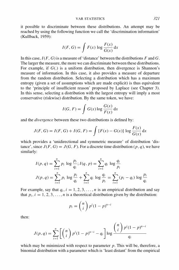
VAR STATISTICS 321
it possible to discriminate between these distributions. An attempt may bereached by using the following function we call the ‘discrimination information’(Kullback, 1959):
I (F, G) =∫
F(x) logF(x)
G(x)dx
In this case, I (F, G) is a measure of ‘distance’ between the distributions F and G.The larger the measure, the more we can discriminate between these distributions.For example, if G(.) is a uniform distribution, then divergence is Shannon’smeasure of information. In this case, it also provides a measure of departurefrom the random distribution. Selecting a distribution which has a maximumentropy (given a set of assumptions which are made explicit) is thus equivalentto the ‘principle of insufficient reason’ proposed by Laplace (see Chapter 3).In this sense, selecting a distribution with the largest entropy will imply a mostconservative (riskwise) distribution. By the same token, we have:
I (G, F) =∫
G(x) logG(x)
F(x)dx
and the divergence between these two distributions is defined by:
J (F, G) = I (F, G) + I (G, F) =∫
[F(x) − G(x)] logF(x)
G(x)dx
which provides a ‘unidirectional and symmetric measure’ of distribution ‘dis-tance’, since J (F, G) = J (G, F). For a discrete time distribution (p, q), we havesimilarly:
I (p, q) =n∑
i=1
pi logpi
qi; I (q, p) =
n∑
i=1
qi logqi
pi
J (p, q) =n∑
i=1
pi logpi
qi+
n∑
i=1
qi logqi
pi=
n∑
i=1
(pi − qi ) logpi
qi
For example, say that qi , i = 1, 2, 3, . . . , n is an empirical distribution and saythat pi , i = 1, 2, 3, . . . , n is a theoretical distribution given by the distribution:
pi =(
ni
)pi (1 − p)n−i
then:
J (p, q) =n∑
i=1
[(ni
)pi (1 − p)n−i − qi
]log
(ni
)pi (1 − p)n−i
qi
which may be minimized with respect to parameter p. This will be, therefore, abinomial distribution with a parameter which is ‘least distant’ from the empirical

322 VALUE AT RISK AND RISK MANAGEMENT
distribution. For a bivariate state distribution, we have similarly:
I (p, q) =m∑
j=1
n∑
i=1
pij log
(pij
qij
); J (p, q) =
m∑
j=1
n∑
i=1
(pij − qij) log
(pij
qij
)
while, for continuous distributions, we have also:
I (F, G) =∫∫
F(x, y) logF(x, y)
G(x, y)dx dy
as well as:
J (F, G) =∫∫
[F(x, y) − G(x, y)] logF(x, y)
G(x, y)dx dy
This distribution may then be used to provide ‘divergence-distance’ measuresbetween empirically observed and theoretical distributions.
The maximization of divergence or entropy can be applied to constructing amultivariate risk model. For example, assume that a nonnegative random vari-able θ has a known mean given by θ , the maximum entropy distribution for acontinuous-state distribution is given by solution of the following optimizationproblem:
Max H = −∞∫
0
f (θ ) log [ f (θ )] dθ
subject to:∞∫
0
f (θ ) dθ = 1,θ =∞∫
0
θ f (θ ) dθ
The solution of this problem, based on the calculus of variations, yields an expo-nential distribution. In other words,
f (θ ) = 1
θe−θ/θ , θ ≥ 0
When the variance of a distribution is specified as well, it can be shown that theresulting distribution is the Normal distribution with specified mean and specifiedvariance. The resulting optimization problem is:
Max H =∞∫
−∞f (θ ) log
1
[ f (θ )]dθ
subject to:∞∫
−∞f (θ ) dθ = 1, θ =
∞∫
−∞θ f (θ ) dθ, σ 2 =
∞∫
−∞(θ − θ )2 f (θ ) dθ

VAR STATISTICS 323
which yields (as stated above) the normal probability distribution with mean andvariance
(θ , σ 2
). If an empirical distribution is available, then, of course, we can
use the divergence to minimize the distance between these distributions by theappropriate selection of the theoretical parameters. This approach can be appliedequally when the probability distribution is discrete, bounded, multivariate distri-butions with specified marginal distributions etc. In particular, it is interesting topoint out that the maximum entropy of a multivariate distribution with specifiedmean and known variance–covariance matrix turns out also to be a multivari-ate normal, implying that the Normal is the most random distribution that has aspecified mean and a specified variance. Evidently, if we also specify leptokurticparameters the distribution will not be Normal.
Example: A maximum entropy price process:Consider a bivariate probability distribution (or a price stochastic process)h(x, t), x ∈ [0, ∞) , t ∈ [a, b]. The maximum entropy criterion can be writtenas an optimization problem, maximizing:
Max H =∞∫
0
b∫
a
h(x, t) log1
[h(x, t)]dt dx
Subject to partial information regarding the distribution h(x, t), x ∈ [0, ∞) , t ∈[a, b]. Say that at the final time b, the price of a stock is for sure Xb whileinitially it is given by Xa . Further, let the average price over the relevant timeinterval be known and given by X (a,b), this may be translated into the followingconstraints:
h(Xa, a) = 1, h(Xb, b) = 1 and1
b − a
b∫
a
∞∫
0
xh(x, t) dx dt = X (a,b)
to be accounted for in the entropy optimization problem. Of course, we can includeadditional constraints when more information is available. Thus, the maximumentropy approach can be used as an ‘alternative rationality’ to constructing proba-bility risk models (and thereby modelling the uncertainty we face and computingits VaR measure) when the burden of explicit hypothesis formulation or the jus-tification of the model at hand is too heavy.
Problem: The maximum entropy distribution with specified marginalsDefine the maximum entropy of the joint distribution by specifying the marginaldistributions as constraints. Or
Max H = −∞∫
0
b∫
a
F(x, y) log [F(x, y)] dy dx

324 VALUE AT RISK AND RISK MANAGEMENT
subject to:
F1(x) =b∫
a
F(x, y) dy; F2(y) =∞∫
0
F(x, y) dx
and apply the multivariate calculus of variations to determine the correspondingdistribution.
10.3.6 Monte Carlo simulation and VaR
Monte Carlo simulation techniques are both widely practised and easy to apply.However, applications of simulation should be made critically and carefully. Insimulation, one generates a large number of market scenarios that follow the sameunderlying distribution. For each scenario the value of the position is calculatedand recorded. The simulated values form a probability distribution for the valueof a portfolio which is used in deriving the VaR figures. It is clear that by usingMonte Carlo techniques one can overcome approaches based solely on a Normalunderlying distribution. While such distributions are easy to implement, thereis an emerging need for better models, more precise, replicating closely marketmoves. But where can one find these models? Underlying distributions are essen-tially derived from historical data and the stochastic model used to interpret data.The same historical data can lead to very different values-at-risk, under differ-ent statistical models, however. This leads to the question: what model and whatdistribution to select? Monte Carlo simulation does not resolve these problemsbut provides a broader set of models and distributions we can select from. In thissense, in simulation the GIGO (garbage in, garbage out) principle must also becarefully apprehended. The construction of a good risk model is by no meansa simple task, but one that requires careful thinking, theoretical knowledge andpreferably an extensive and reliable body of statistical information.
10.4 VaR EFFICIENCY
10.4.1 VaR and portfolio risk efficiency with normal returns
VaR, either as an objective or as a risk constraint, has become another tool forthe design of portfolios. Gourieroux et al. (2000), Basak and Shapiro (2001) haveattracted attention to this potential usefulness of the VaR. To see how VaR-efficientportfolios can be formulated we proceed as follows: let Wt (.) be the value of aportfolio at time t and let, at a time t + h later, wealth be Wt+h(.). The probabilityof the value at risk in the time interval (t, t + h) is then given by:
Pr [Wt+h − Wt < −VarW (h)] = PVaR
Thus, if the return is RW (h) = Wt+h − Wt we can write instead:
Pr [RW (h) < −VarW (h)] = PVaR

VAR EFFICIENCY 325
Models will thus vary according to the return model used in value at risk estima-tion. For our purposes, let N be the number of financial assets, P(i, t) be the priceof asset i at time t and B(t) be the budget at time t . We also set a1, a2, a3, . . . , aN
be the number of shares held of each asset at time t . As a result, the wealth stateat time t is:
Wt (a) =n∑
i=1
ai pi,t = aT pt
while the return in a time interval is:
Wt+1(a) − Wt (a) = aT (pt+1 − pt )
The loss probability α = PVaR implies a VaR calculated in terms of the portfolioholdings and the risk constraint, or VaRt (a, α) is defined by:
Pt [Wt+1(a) − Wt (a) < −VaRt (a, α)] = α
where Pt is the conditional distribution of future asset prices given the informa-tion available at time t . Set the price change yt+1 = pt+1 − pt . Then we haveequivalently,
Pt [−aT yt+1 > VaRt (a, α)] = α
In other words, the portfolio VaR is determined in terms of information regardingpast prices, the portfolio composition and the specified loss probability α. Whenthe price changes are normally distributed:
yt+1 ∼ N (µt , t ) then VaRt (a, α) = −aT µt + (aT t a
)1/2Z1−α
where Z1−α is the 1 − α quantile of the standard normal distribution. We mightconsider then a number of portfolio design approaches.
Problem 1Maximize expected returns subject to a VaR constraint.
Problem 2Minimize a VaR risk subject to returns constraints.The first problem is stated as follows:
Maxa
E(aT yt+1
)subject to VaRt (a, α) ≤ VaR0
where VaR0 is a VaR constraint specified by management. The solution of thisproblem will turn out to be a portfolio allocation which is necessarily a functionof the risk parameters α, VaR0. By the same token, we can state the secondproblem as follows:
Mina
VaRt (a, α) subject to E(aT yt+1
) ≥ R
where R is the required mean return. A solution to these problems by analyticalor numerical means is straightforward.

326 VALUE AT RISK AND RISK MANAGEMENT
10.4.2 VaR and regret
The Savage (1954) regret criterion has inspired a number of approaches called‘regret–disappointments models’ (Loomes and Sugden, 1982, 1987). Accordingto Bell (1982), disappointment is a psychological reaction to an outcome thatdoes not meet a decision maker’s expectation. In particular, Bell assumed that themeasurement of disappointment is assumed to be proportional to the differencebetween expectation and the outcome below the expectation. Elation, may occurwhen the outcome obtained is better than its expectation. Usually (for risk-aversedecision makers), the ‘cost of reaching the wrong decision’ (disappointment) maybe, proportionately, greater than the payoff of having made the right decision(elation). In other words, managers abhor losses, valuing them more than theyvalue gains for having made the right decision. The inverse may also be true. Atrader whose income is derived from trade-ins only may be tempted to assumerisks which may be larger than the investment firm may be willing to assume.For example, a stock performance below that expected by analysts can havedisproportionate effects on stock values while an uncontrollable trader may leadto disaster. To see how to proceed, consider the utility of an investment given byu(x) and let CE be its certainty equivalent. That is to say, as we saw in Chapter 3:
u(CE) = Eu(x) and CE = u−1 [Eu(x)]
Say that ‘disappointment’ occurs when the outcome is below CE, resulting in anexpected utility that is depreciated due to disappointment. As a result, an adjustedexpected utility, written by V (b) with a factor b can be specified by:
V (b) = Eu(x) − bE [u(C E) − u(x) |C E ≥ x ]
Explicitly, it equals the expected utility less the expected utility loss when theex-post event is below the certainty equivalent,
V (b) = Eu(x) − b [Eu(x) − u(x) |C E ≥ x ]
Since Eu(x) = u(C E), we also have:
V (b) = Eu(x) − b [u(C E) − u(x) |C E ≥ x ]
= u(C E) (1 − bF(C E)) + bEu (x |x ≤ C E )
This procedure allows us to resolve the problem of a reference point endoge-nously. For example, consider a two-event process:
x = (x1, x2) with prob (α,1 − α) with x1 > x2
which corresponds to a binomial model. Then, the expected utility is:
Eu(x) = u(C E) = αu(x1) + (1 − α)u(x2)
while
V (b) = [αu(x1) + (1 − α)u(x2)] [1 − b(1 − α)] + bu(x2)(1 − α)
and therefore:
V (b) = α [1 − b(1 − α)] u(x1) + (1 − α) (1 + bα) u(x2)

REFERENCES AND ADDITIONAL READING 327
which we can write as follows:
V (b) = αβu(x1) + (1 − α) (β + b) u(x2); β = [1 − b(1 − α)]
Since b > 0, it provides a greater weight to the lower outcome. Further,
= V (b) − Eu(x) = (1 − β) [u(x1) − αu(x2)]
By applying the same argument to the VaR by assuming a linear truncated utility,we have:
V (b, VaR) = E(x) + bE [−VaR + x |−VaR > x ]
As a result, the expected value is:
V (b, VaR) = E(x) + b
−VaR∫
−∞(x − VaR) dF(x)
For example, say that an option price is C(0) while the strike price over one periodis K and assume two states x1, x2, x1 ≤ K ≤ x2. Thus, the expected value of theoption price is:
C(0) = 1
1 + r
α
1 + b(1 − α)u(0) + (1 + b)(1 − α)
1 + b(1 − α)u(x2 − K )
If the option price can be observed together with the utility of u(0), then theequivalent parameter b is found to be equal to:
0 < b = αu(0) + (1 − α)u(x2 − K ) − C(0)(1 + r )
(1 − α) [C(0)(1 + r ) − u(x2 − K )]
Note that αu(0) + (1 − α)u(x2 − K ) < C(0)(1 + r ), meaning that we require fora positive disappointment parameter (since we have necessarily, C(0)(1 + r ) <
u(x2 − K )) that the option price be larger than the expected value of the utilityof the option lottery. In other words, the option price also includes the investor’sdesire for the potential to reduce deception by allowing him to regret and reversea decision badly taken.
REFERENCES AND ADDITIONAL READING
Alexander, C.O. (1998) The Handbook of Risk Management and Analysis, John Wiley & Sons,Inc., New York.
Arrow, K.J. (1971) Essays in the Theory of Risk Bearing, Markham, Chicago.Artzner, P., F. Delbaen, J.M. Eber and D. Heath (1997) Thinking coherently, Risk, 10, 67–71.Artzner, P., F. Delbaen, J. Elber and D. Heath (1999) coherent measures of risk, Mathematical
Finance, 9, 203–228.Basak, S., and A. Shapiro (2001) Value-at-risk-based risk management: Optimal policies and
asset prices, The Review of Financial Studies, 14, 371–405.Basle Committee (1996) Amendment to the capital accord to incorporate market risks, on
banking supervision, January.

328 VALUE AT RISK AND RISK MANAGEMENT
Bauer, C. (2000) Value at risk using hyperbolic distributions, Journal of Economics and Busi-ness, 52, 455–467.
Bell, D.E. (1982) Regret in decision making under uncertainty, Operations Research, 30,961–981.
Bell, D.E. (1983) Risk premiums for decision regrets, Management Science, 29, 1156–1166.Bell, D.E. (1985) Disappointment in decision making under uncertainty, Operation Research,
33, 1–27.Cvitanic, J., and I. Karatsas (1999) On dynamic measures of risk, Finance and Stochastics, 3,
451–482.Dowd, K. (1998) Beyond Value at Risk, The New Science of Risk Management, John Wiley &
Sons, Ltd, Chichester.Duffie, D., and J. Pan (1997) An overview of value at risk, Journal of Derivatives, 4, 7–49.Embrecht, P., A. Hoing and A. Juri (2001) Recent advances in the application of copulae to
non-linear Value at Risk, ETH Department of Mathematics, CH-8092 Zurich, April.Embrecht, P., C. Kluppelberg and T. Mikosch (1997) Modelling Extremal Events, Springer-
Verlag, Berlin.Feller, W. (1957, 1966) An Introduction to Probability Theory and its Applications, Vols 1 and
2, John Wiley & Sons, Inc., New York.Fishburn, P. (1977) Mean risk analysis with risk associated with below target returns, American
Economic Review, 67(2), 116–126.Gourieroux, C., J.P. Laurent and O. Scaillet (2000) Sensitivity analysis of values at risk, Journal
of Empirical Finance, 7, 225–245.Gul, Faruk (1991) A theory of disappointment aversion, Econometrica, 59, 667–686.Jia, J., and J.S. Dyer (1994) Risk-value theory, Department of Management Science and In-
formation Systems, The Graduate School of Business, University of Texas, Austin, WP,94/95-3-4.
Jorion, P. (1997) Value at Risk: The New Benchmark for Controlling Market Risk, McGraw-Hill,Chicago.
Jorion, P. (1999) Risk management lessons from long term capital management, Working Paper,University of California, Irvine.
Kullback S. (1959) Information Theory and Statistics, Wiley, New York.Loomes, G., and R. Sugden (1982) Regret theory: An alternative to rational choice under
uncertainty, Economic Journal, 92, 805–824.Loomes, G., and R. Sugden (1987) Some implications of a more general form of regret theory,
Journal of Economic Theory, 41, 270–287.Morgan, J.P. (1995) Introduction to RiskMetricsT M , 4th Edition, November.Robinson, Gary (1995) Directeur, R&D Division, Global Market Risk Management, BZW,
Value-at-Risk Analysis: Its Strengths and Limitations, October.Savage, L.J. (1954) The Foundations of Statistics, John Wiley & Sons, Inc., New York.Schachter, B. (2002) All about value at risk, www.GloriaMundi.org/var.Shiu, E.W. (1999) Discussion of Philippe Artzner’s, ‘Application of coherent risk measures to
capital requirements in insurance’, North American Actuarial Journal, 3(2).Shore, H. (1986) Simple general approximations for a random variable and its inverse distri-
bution function based on linear transformations of nonskewed variate, SIAM Journal onScientific and Statistical Computing, 7, 1–23.
Shore, H. (1995) Identifying a two parameter distribution by the first two sample moments(partial and complete), Journal of Statistical and Computational Simulation, 52, 17–32.
Stone, B. (1973) A general class of three parameter risk measures, Journal of Finance, 28,675–685.
Tapiero, C.S. (2003) VaR and inventory control, European Journal of Operations Research,forthcoming.
Telser, L.G. (1956) Safety first and hedging, Review of Economic Studies, 23, 1–16.

Author Index
Akerlof, G. 68, 226Allais’ Paradox 52–3Amikam, Meir 199Aquila 197Arnold, L. 92Arrow, K.J. 44, 212Artzner, P. 309, 310Augustine, St 273
Bachelier, L. 16, 84Barrois, T. 7Basak, S. 324Bell, D.E. 29, 326Bensoussan, A. 92, 139, 154Bismut, J.M. 92Black, F. 226, 252Bloomberg 300Bolder, David 253Bollerslev, T. 280Borch, K.H. 8Born, M. 79Broadie, M. 154Brock, W.A. 92Brown, Robert 88
Capocelli, R.M. 209Cardano, Girolamo 81–2Carr, P. 154, 157Cochrane, John H. 66, 67Connolly, K.B. 184Cotton, Peter 258Cox, D.R. 92, 192, 296Cox, J.C. 226Cox–Ingersoll–Ross (CIR) model 257Cramer, Gabriel 51–2Cramer, H. 8Cvitanic, J. 309
Darling, D.A. 209Delbaen, F. 253Detemple, J. 154Dixon, Hugo 68Donsker Theorem 99–100Doob, J.L. 82Duff & Phelps 12Duffie, G.R. 230
Eeckoudt, L. 44Einstein, Albert 84Elliot, R.J. 92Embrecht, P. 319Engle, R.F. 280
Fama, E.F. 88, 112, 274Feller, W. 51–2, 194Fielitz, B. 301Filipovic, D. 253Fishburn, P. 309Fisher, Irving 212Fisher, R.A. 6Fokker–Planck equation 88Foster, D.P. 280Fouque, Jean-Pierre 258Friedman, Milton 112
Ghashghaie, S. 80Goldman, M.B. 184Gourieroux, C. 324Green, M.T. 301
Hogan, M. and Weintraub, K. 252Hoing, A. 319Huang, J. 154Hull, J. 258Hurst, H.E. 300
Risk and Financial Management: Mathematical and Computational Methods. C. TapieroC© 2004 John Wiley & Sons, Ltd ISBN: 0-470-84908-8

330 AUTHOR INDEX
Ito, K. 92
Jarrow, R. 227, 242Jorion, P. 310Julien, H. 139Juri, A. 319
Kahnemann, D. 53Kalman, R.E. 79Kappa 183Karasinski, P. 252Karatzas, I. 309Kay, John 9Kim, I.J. 156–7Kimball, M. 44, 45Kluppenberg, C. 319Koch 197Kolmogorov 79, 84Kortanek, K.O. 253Kullback, S. 291, 321
Leeson, Nick 202Leland, H.E. 226Levy, P. 82, 84Lintner, J. 63Lo, Andrew W. 272Longstaff, F. 226Loomes, G. 29, 326Lorenz, Edward 79, 80Lorimier, S. 253Lucas, R.E. 112, 113Luce, R.D. 7Lundberg, F. 8
Machina, M.J. 53Magill, M. 111, 212Malkiel, Burton 13Malliaris, A.G. 92Mandelbrot, B. 88, 272,
300, 301Markowitz, Harry 62–3McKean, H.P. 92Medvedev, V.G. 253Merrill Lynch 68, 200Merton, R.C. 153, 226Mikosch, T. 319Miller, H.D. 92, 192Miller, M.H. 112Milshtein, G.N. 100
Morgan, J.P. 197, 200Morgenstern Oskar, 41Muth, John 111, 112, 293
Nelson, C.R. and Siegel, A.F., approach tointerest rates 253
Nelson, Daniel 96, 280Nelson, Erick 199
Papanicolaou, George 258Pearson, Karl 6Pliska, S.R. 139, 146Pratt, J.W. 44
Quiggin, J. 53Quinzii, M. 111, 212
Raiffa, H. 7Ramaswamy, K. 96Reyniers, D. 73, 75Ricciardi, L.M. 209Roll, Richard 112Rubinstein, Ariel 20
Samuelson Paul 112Sandmann, K. 252Sargent, T.J. 112Savage, L.J. 29Schlaiffer, R. 7Schwartz, E. 226Shapiro, A. 324Sharpe, William 63Shiu, E.W. 310Shreve S.E. 139Siegel, A.F. 253Siegert, A.J.F. 209Singleton, K.J. 230Sircar, K. Ronnie 258Sklar 319Sonderman, D. 252Soros, George 84Spence, M. 72Stone, B. 309Sugden, R. 29, 326Svensson 253Szekely, Gabor 82
Tapiero, Charles 92, 257Taylor H.M. 280

AUTHOR INDEX 331
Tetens, J.N. 7Tobin, James 63Turnbull, S. 227Tverski, A. 53
Van Ness, J.W. 301Vasicek 254–8, 258Ville, J. 82Von Neumann John 41
Walras, L. 212Weatherstone, Dennis 310Wets, Roger J.B. 253White, A. 258Wiener, Norbert 84Willasen, Y. 45Wilmott, P. 182, 183, 262
Yu, G. 156–7
Index compiled by Annette Musker

Subject Index
ABN AMRO Asset Management 21, 202absolute risk aversion, index of 44absorbing state 207accounting rate of return (ARR) 54–5actuarial science, insurance and 7–10adverse selection 68–9, 71affine structure 254, 255affine term structure (ATS) model 261Allais’ Paradox 52–3Allied Irish Bank (AIB) 24AMBAC 231American call option 116American put option 149, 154–7AMEX 118Aquila 197arbitrage 6, 119, 277
arbitrage-based strategies 121–2arbitrage pricing theory (APT) 64
ARCH 7, 80, 278, 280, 282Arrow–Debreu paradigm 277Arrow–Pratt index of risk aversion 45, 47Artificial Intelligence 15Asian financial crisis 70autocovariance function 91
Baltic Exchange (London) 116Bank of Canada 253Bankers Trust 199–200barrier option 164–5basis risk 115Basle Committee 310–11, 313Bayes criterion 26–7Bayes decision making 22–6Bayes theory 7Bayesian rationality 22bear spread 162, 179Bermudan option 118Bernouilli, Daniel 51–2
beta factor 60, 61, 63binomial random walk 96binomial tree, multi-period 140–1black sheep syndrome 21Black–Scholes option formula 6, 147–57,
168, 196volatility and 281
bond(s)arbitrageurs 214convertible 114, 261–2corporate 217coupon-bearing 215–17default 216, 224–30definition 211fixed rate 211floating rate 211forward rate and 222–4junk 216markets 212mathematics 218options on 260–4, 268–9ratings 231risk 161strips 211valuation, interest-rate processes, yields
and 251–9see also rated bonds
bonus-malus 8bounded rationality 4, 19, 20–2bounds, option 152–3Brownian motion 16, 80, 88, 92, 99–100bull spread 162, 178–9butterfly effect 80butterfly spread 162, 181
calendar spread 162call–call spread strategy 178call option 116, 117, 133–4, 149, 169, 172–4
Risk and Financial Management: Mathematical and Computational Methods. C. TapieroC© 2004 John Wiley & Sons, Ltd ISBN: 0-470-84908-8

334 SUBJECT INDEX
call option price 135calls on calls 164calls on forwards 164calls on puts 164cap 117, 163, 262capital adequacy ratio (CAR) 310capital adequacy requirements (CAR) 12,
13, 73Capital Asset Pricing Model (CAPM) 54, 56,
187capital markets and 63–4investment and 59–61risk-premium and 295
capital market equilibrium 56caplet 262caption 163, 264cash or nothing 163CBOE 117Central Limit Theorem 16certain cash equivalent 57certainty equivalence 43–4, 45certification 271CFTC 126, 127chaos 79–80chaotic analysis 272cherry-picking 71Chicago Board of Trade (CBOT) 114, 117Chicago Mercantile Exchange (CME) 13,
114, 117, 126, 197chooser option 164claims 8classical discounting 65classical rationality 21climatic option 163climatic risks 196–7collar 262collateral call 124Commodity Exchange Act 125Commodity Futures Trading Commission
170commodity option 163, 169commodity pool 125commodity pool operators (CPOs) 125competition risk 11complete market 119, 146complexity analysis 272compound option 162, 165–70Computational Tool 15condor 162condor spread strategies 81
consumption, individual investment and57–9
contingent claim assets 114contract 114control 24convertible bond 114, 261–2convertible preferred stock 114convex dominance 272convexity 218–22copula distributions 315, 318–19corporate bond 217correlation analysis 122correlation coefficient 91, 92correlation function 91correlation risk 197corridor (range note) 163, 262counter strategies of hedge funds 124coupon-bearing bond 215–17coverage 225covered call 162, 176–7Cox–Ingersoll–Ross (CIR) model 257credit ratings, downgrading 231–2credit risk 12–13crowd psychology 21cubic utility function 47currency option 163currency risk 12
Daiwa Bank 13data mining 3, 15dead value 141death spiral 200decision criteria 26–31Decision Making Under Uncertainty
(DMUU) 4, 7decision table 31–3default bond 216
risky debt and 224–30default, definition 227–8default rate 225degree of absolute prudence 45delivery price of stock 141Delta 151, 174, 182, 199dependencies 8, 9derivative asset 114derivative contract 114derivative security 6derivatives losses 198destabilizing strategies of hedge funds 124deterministic analysis 34

SUBJECT INDEX 335
Deutsche Bank 202Deutsche Terminbrose (DTB) 118diffusion–stochastic differential equation
models 96diffusion–volatility 89disappointment 326–7discrete time approximations 100–3discrimination information 321divergence-distance measures 322diversification, principle of 62Donsker Theorem 99–100downside risk 309duration 218–22, 309dynamic hedging 124Dynegy Inc. 231
efficient markets hypothesis 89endowment effect 21Enron 69, 197, 232entropy, maximum, principle of 320–4
discrimination and divergence 320–3distribution with specified marginals
323–4price process 323
environmental litigation 67environmental protection 25environmental risk 9–10, 196–7EOE (European Options Exchange,
Amsterdam) 118equally likely (Laplace) criteria 34equilibrium 293–5error normality 88Euler equation 65–7
equilibrium and 293–5Eurodollar deposits 162European call option 116, 148, 149European Monetary System 120event-related funds 123ex-ante risk management 23excess discount rate 56exchange option 163, 164exercise date 116exercise value 141expectation criterion 43expected cost criterion 32expected monetary cost 32Expected Monetary Value (EMV) 26–7,
33–7, 39, 40expected opportunity loss (EOL) 33–7expected payoff criterion 32
Expected Profit under Perfect Information(EPPI) 33–7
expected utility 40, 41, 45bounds 45–6critiques of 51–3finance and 53–67insurance, risk management and 48–50
expected value (Bayes) criterion 26–7expected value of sample information
(EVSI) 33–7exponential utility function 46–7ex-post risk management 23
fair competition 67fair game 81–2‘fallen angels’ 225fat tails 81, 89, 272FGIC 231filter rule 191financial instruments 113–19financial physics 15–16finite difference model 103firm liquidity 8First Boston 200first passage time 207–9Fitch Investor Service 12, 217fixed equivalence rate of return (FIE) 55flexibility 29flipping 70floating rate bond 211floor 117, 163, 262floorlet 262floortion 264Fokker–Planck equation 88forcing contract 75forecasts, optimal, rational expectations and
146–7foreign exchange (FX) trading 195
price of a European call option on 196–7foreign exchange risk 10–11forward contract 114–16, 141–5forward rate agreement (FRA) 115–16forward rate, bonds and 222–4forward starts 162fractional Brownian motion 272, 301franchises 75Frechet distribution 312, 317Freddie Mac 203front-running 70FSA 231

336 SUBJECT INDEX
fundamental factor model 64fundamental theorem of asset pricing 83fundamental theory, definition 3funding risk 201futures
contract 114–16, 141–5market 115occurrences, example 145price 143–4
gambler’s ruin problem 191gambling 81–2Gambling Act (1774) 8Gamma 151, 182GARCH 7, 80, 278, 280, 282generalized method of moments (stochastic
discount factor; SDF) 54, 65–7, 113,274
genetic testing, insurance and 71Gibson Greeting 199–200Girsanov Theorem 104–8Granite Partners 203‘Greeks’ 151–2, 174
dynamic strategies and 181–4Gumbel distribution 317
HARA (hyperbolic absolute risk aversion)47
hazard rate dominance 272hedge fund fees 127hedge funds 120–5hedging 6, 119, 120–3hedging portfolio 6herd effect index 301herding 21, 124–5holding cost 139homogeneity of reserves 310Hong Kong Futures Exchange 118Hurst exponent 300, 301
IBM 198immediacy, financial instruments and 5immunization 221–2in the money (ITM) 151incentive compatibility constraint 75incompleteness in pricing 276, 277–8independent increments 92individual rationality constraint 75inflation 14–15inflation risk 14, 15
information asymmetry 67–75, 113insider trading 113insufficient reason (Laplace), principle of 27,
321insurance 24
actuarial science and 7–10contract 8
interest rate modelling 251–3interest rate swap 262–4interest rates and term structure 259, 267–8internal rate of return (IRR) 55International Monetary Fund (IMF) 70invariance by drift 310investor protection rules 125–7irrational behaviour 39Ito’s Lemma 93–4, 147, 148, 170, 191, 251,
252applications of 94–108application to wealth process of portfolio
of stocks 95–6
Jensen’s inequality 45, 46Joseph effect 300junk bonds 216Junk–Treasury Spread (JTS) 224, 225
knock-out option 162Kolmogorov 79, 84Kolmogorov (Fokker–Plank) equation 208
Laplace (equally likely) criteria 34Laplace principle of insufficient reason 27,
321Laplace transform 208laps and flex 162law of the single price 24, 83, 84, 134, 146least divergence, principle of 288lemon phenomenon 68–9leptokurtic distributions 81, 88, 89leverage, hedge fund and 127linear growth of uncertainty 272linear regression 7linear risk-sharing rule 74Lipschitz conditions 90, 91liquidity 5liquidity risk 14logarithmic utility function 47London International Financial Futures
Exchange (LIFFE) 118, 197London’s Baltic Exchange 116

SUBJECT INDEX 337
long call option 172long put option 174Long-Term Capital Management (LTCM)
120lookback option 163loss prevention 24–5loss rate 225lotteries, utility functions and 40–2lower bounds of option 152Lyapunov stability analysis 272
macro funds 121macro hedged funds 121macro specific fund strategies 122macroeconomic approach 64man-made risks 8, 9margin calls 124Marine Stewardship Council (MSC) 271market efficiency 112–13, 184
market memory and 274market fluctuations risk 201market gladiators 161, 162market hedge funds 123market inefficiencies 25, 184–5market integrity protection rules of hedge
funds 126market rationality 123market risk 14Markov chain 96, 224, 230Markov stochastic process 89martingale 82–3
Girsanov Theorem and 104–8market efficiency and 112Wiener process as 106–7
MATHEMATICA 152MATIF (Marché à Terme International de
France) 118MATLAB 152maturity 141maximax (minimin) criterion 28, 34maximin (minimax) criterion 28, 34MBIA 231mean variance replication hedging 288–91mean reversion model 252memory, volatility and 273–4Merrill Lynch 68, 200Merton model 170, 251, 297–9Metalgesellschaft (MG) 201–2
MG Refining & Marketing (MGRM)201–2
minimax (maximin) criterion 28minimax regret 28–31, 334minimin (maximax) criterion 28min-max objectives 26monotonicity 310Monte Carlo simulation 163
VaR and 324Moody’s 12, 212, 217, 224, 225, 227
bond ratings 231, 232moral hazard 25, 69–71multifractal time series analysis 272multiple-factor model 64mutual funds regulation 127
net present value (NPV) 55–6, 217–18network and information asymmetries 277neural networks 3New York Federal Reserve Bank 200New York Mercantile Exchange (NYMEX)
201New York Stock Exchange (NYSE) 70, 118Nikkei Index 202–3Nippon Investor Service 12no arbitrage assumption 134, 135, 241, 242nonlinear (non-Gaussian) distributions 81non-Gaussian distributions 81non-uniqueness in pricing 276Normal distribution 88, 89–90, 312, 322–3Normal–Wiener processes 89numeraire 137
obligation to sell 116offshore funds 162one-factor models (market premium in the
CAPM) 63–4opportunity loss 3opportunity loss table 32–3, 35option misses 197–204option writers 161option(s) 13, 114, 116–19
asset or nothing 163as you like it 165Asian 118, 162, 164barrier 164–5Bermudan 118on bonds 260–4, 268–9bounds 152–3call 116, 117, 133–4, 148, 149, 169, 172–4chooser 164climatic 163

338 SUBJECT INDEX
option(s) (Cont.)commodity 163, 169on corporate bonds 162currency 163on dividend-paying stocks 169exchange 163, 164on foreign currencies 169on futures 163, 170on a futures price 170jump processes and 297–9knockout 162long call 172lookback 163on options 164over-the-counter 118packaged 162, 163–5passport 165path-dependent 162practice and 171–84rational expectations 135–7stock 162, 165–70upper bounds of 153valuation 131–41value at risk,, by Delta–Gamma 317–18see also put options
Orange County (California) case 199, 200–1Ornstein–Uhlenbeck process 97, 254, 297
application of Ito’s Lemma to 94–5Osaka Stock Exchange (OSE) 203out of the money (OTM) 21, 151over-insurance 25over-the-counter (OTC) derivatives 114over-the-counter option 118
packaged option 162, 163–5Pareto–Levy distributions 88, 89Pareto optimal risk sharing 74participation constraint 75passport option 165path-dependent options 162payback period 54payments based in effort 75payoff table 29, 31Philadelphia Exchange 195, 196PHLX 118plain vanilla strategies 172–5planning experiments 6–7platokurtic distributions 88Poisson Jump 92positive feedback trading 124
power utility function 47predictability of markets 274preferred probability distribution 53premium 116premium payments 8, 48–50premium principles 8prepayment risk 122present value 12price risk 197PriceWaterhouseCoopers 203pricing and classical contract theory 277pricing insurance 8principal–agent problem 73–5private placements 125probabilistic analysis 34–7Procter & Gamble 199–200production-efficiency function 25proper hedge risk 201protective put 124, 162, 177prudence 44–5psychology and rationality 277–8put option 116, 117, 169, 172–4, 175
American 149, 154–7buying 177calls on 164long 174protective 124, 162, 177
put–call parity 153, 165puts on calls 164
quadratic utility function 47quantile risk see value at risk (VaR)quantity risk 197quantos 163
R/S index 300, 301random cash flows 55–6random walk 84–91, 272, 282randomness, definition 79range 309range note 163, 262range to scale (R/S) analysis 272, 273rare events 8–9rated bond 212, 216
default and 230–51duration 235–9Markov chain and 233–5pricing for risk-free rates 239–44
no-arbitrage condition 241–2valuation of two-rates rated bond 242–4
SUBJECT INDEX 339
valuation of default-prone rated bonds244–51
cash value of rated firm 250–1two-rated default bond 248–9
rational expectations 21–2, 83–4, 111–13,131
optimal forecasts and 146–7rationality, principles of 4, 20–2recovery ratio 226reduced-form models of default 226,
227–8cf structural models 228–30
reflexivity 84regret (Savage regret) 28–31
ex-post optimization and 26valuation of firms and 30VaR and 326–7
regret–disappointments models 326reinsurance 49remembering 274repos 211reverse mortgage 215reward 40rho 151right to exercise 116risk aversion 43–5risk behaviour, utility and 42–8risk, definition 5–6, 23, 309risk diversification 24risk loving 43risk management 22, 23–6Risk Metrics 318risk-neutral pricing 22, 53, 112, 131, 137–9,
166, 184, 185, 186, 188risk-neutral probabilities 6, 119, 136, 137,
145–7, 167risk-neutral world 142–3risk premium 24, 43–4, 45risk sharing 8, 47–8, 49risk tolerance 42risk transfer 49robustness 23, 25–6, 44–5
Savage regret criterion see regretscenario analysis 31–3, 122scenario optimization 26, 62screening 72–3, 277SEC 126sector funds 123sector risk 14
Security Exchange Act (SEA) 126self-selection constraints 72–3semi-variance 309sensitivity equations 151–2September 11th, 2001 9sequentiality 274Shannon’s entropy 320, 321shape risk 14short selling 123, 174signalling –3SIMEX (Singapore International)
118, 203smile 6, 151smoothing splines 253Société Générale 313Southern Energy 197spatial diversification 5speculation 119Spence, M. 72spillover events 9spread strategies 178–9square root process 257St Petersburg Paradox 51–2stabilizing strategies of hedge funds
124stacked rollover hedge 201Standard & Poors 12, 212, 217, 224, 227,
231state discretization 96–9stationarity 91–2statistical approach, APT and 64statistical data analysis 6stochastic calculus 92–4stochastic differential equations (SDEs) 88,
89, 90, 96stochastic discount factor (SDF)
(generalized method of moments) 54,65–7, 113, 274, 276, 293
stochastic dominance 272stochastic ordering 272stochastic processes, properties of 91–2stochastic volatility binomial models
282–93stochastic volatility interest-rate models
258–9stochastic volatility models 89, 282–93stochastic volatility, process discretization
280–1stock, buying 177stock option 162, 165–70

340 SUBJECT INDEX
stopping time sell and buy strategies 184–95,226
buying/selling on a random walk 189–90pricing a buy/sell strategy on a random
walk 193–5straddle 179, 180strangle 179, 180strap 180–1stress test 122strict stationarity 91strike price 116strip 180, 181strips bonds (Separate Trading of Registered
Interest and Principal of Securities) 211structural models of default 226–7
cf reduced form models 228–30sub-additivity of reserves 310subjective probability distribution 111sub-martingale 82sunk costs 20super-martingale 82supershare 163sure-thing principle 52Svensson procedures 253swaps 117, 163
contracts 196interest rate 262–4
swaption 163, 264switch 163systematic risk 199systemic risk 125
reduction rules of hedge funds 126–7
Taylor series approximation 100, 101Taylor series expansion 93, 151Tchebycheff bounds on expected utility 45technical analysis 273technological innovation 25term structure 56
interest rates and 267–8theta 151, 182Thomson Bank Watch 12time contraction 284–6time (process) discretization of
continuous-time finance models96–103
time phasing of events 5Tokyo International Financial Futures
Exchange (TIFFE) 118
too big to fail syndrome 70Toronto Stock Exchange (TSE) 118trade on volatility 151trading strategy 131traditional valuation 54–6tragedy of the commons 21transaction risk 11transition bond rating matrix 244transivity axiom 42transparency 70Treasury bills 212trinomial walk 96, 191–3truth-in-lending 67two-fund separation theorem 63
upper bounds of option 153utility
concept of 19, 39–42lotteries and 40–2maximization 61–3risk behaviour and 42–8see also expected utility
value at risk (VaR) (quantile risk) 23, 26, 46,185, 199, 309, 310–11
analytic variance–covariance approach315–16
in banking practice 313–14Burr 317copulae and portfolio measurement
318–19definition and applications 311–15efficiency 324–7extreme statistics and 316–17Frechet distribution and 317Gumbel distribution and 317historical approach 315Monte Carlo simulation and 324negentropy 320numerical examples 314–15option, by Delta–Gamma 317–18portfolio risk efficiency with normal
returns and 324–5regret and 326–7statistics 315–24Weibull distribution and 317
value investing funds 123Vasicek interest-rate model 254–8
nonstationary 258

SUBJECT INDEX 341
Vega 151, 174Vivendi Universal SA 231volatility 6, 88
definition 271–3equilibrium and 275–8implicit 281–2incomplete markets and 276–8memory and 273–4modelling and estimation 272–3process variance and 278–81range process and 299–301risk 14smile 281–2
Wald’s identity 190Walras, L. 212
warrants 114, 162, 163, 168–9wealth, definition 8, 131wealth process of portfolio of stocks
application of Ito’s Lemma to 95–6Weibull distribution 312, 317Wiener (Levy) process 88, 90, 92, 95–6
as a martingale 106–7Wiener risk 298‘wild money’ 13Willasen inequalities 46World Bank 162WorldCom Inc. 231
yield curve estimation 24zero-coupon bonds 211zero-coupon, default-free bond 213–14
Index compiled by Annette Musker