Review for Exam2 - University of Iowafluids/Posting/Exams... · 2015-11-13 · Review for Exam2 11....

Review for Exam2

11. 13. 2015

Hyunse Yoon, Ph.D.

Adjunct Assistant ProfessorDepartment of Mechanical Engineering, University of Iowa

Assistant Research ScientistIIHR-Hydroscience & Engineering, University of Iowa

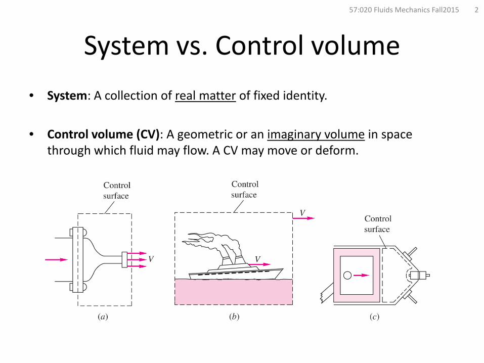
System vs. Control volume• System: A collection of real matter of fixed identity.

• Control volume (CV): A geometric or an imaginary volume in space through which fluid may flow. A CV may move or deform.

57:020 Fluids Mechanics Fall2015 2

Laws of Mechanics for a System57:020 Fluids Mechanics Fall2015 3

Laws of mechanics are written for a system, i.e., for a fixed amount of matter• Conservation of mass

𝐷𝐷𝐷𝐷𝐷𝐷𝐷𝐷

= 0

• Conservation of momentum𝐷𝐷 𝐷𝐷𝑉𝑉𝐷𝐷𝐷𝐷 = 𝐷𝐷𝑎𝑎 = 𝐹𝐹

• Conservation of energy𝐷𝐷𝐷𝐷𝐷𝐷𝐷𝐷 = �̇�𝑄 − �̇�𝑊

Note:𝐷𝐷 𝐷𝐷𝑉𝑉𝐷𝐷𝐷𝐷 = �

𝐷𝐷𝐷𝐷𝐷𝐷𝐷𝐷=0

𝑉𝑉 + 𝐷𝐷 �𝐷𝐷𝑉𝑉𝐷𝐷𝐷𝐷=𝑎𝑎

= 𝐷𝐷𝑎𝑎

Governing Differential Eq. (GDE):

∴𝐷𝐷𝐷𝐷𝐷𝐷 𝐷𝐷,𝐷𝐷𝑉𝑉,𝐷𝐷

system extensiveproperties, 𝐵𝐵sys

= RHS

Reynolds Transport Theorem (RTT)• In fluid mechanics, we are usually interested in a region of space, i.e.,

CV and not particular systems. Therefore, we need to transform GDE’s from a system to a CV, which is accomplished through the use of RTT

𝐷𝐷𝐵𝐵sys𝐷𝐷𝐷𝐷

time rate of changeof 𝐵𝐵 for a system

=𝐷𝐷𝐷𝐷𝐷𝐷

�CV 𝑥𝑥,𝑡𝑡

𝛽𝛽𝛽𝛽𝛽𝛽𝑉𝑉

time rate of changeof 𝐵𝐵 in CV

+ �CS 𝑥𝑥,𝑡𝑡

𝛽𝛽𝛽𝛽𝑉𝑉𝑅𝑅 ⋅ 𝛽𝛽𝐴𝐴

net flux of 𝐵𝐵across CS

where, 𝛽𝛽 = 𝑑𝑑𝐵𝐵𝑑𝑑𝑑𝑑

= 1,𝑉𝑉, 𝑒𝑒 for 𝐵𝐵 = (𝐷𝐷,𝐷𝐷𝑉𝑉,𝐷𝐷)

• Fixed CV,

𝐷𝐷𝐵𝐵sys𝐷𝐷𝐷𝐷 =

𝜕𝜕𝜕𝜕𝐷𝐷 �CV

𝛽𝛽𝛽𝛽𝛽𝛽𝑉𝑉 + �CS𝛽𝛽𝛽𝛽𝑉𝑉 ⋅ 𝛽𝛽𝐴𝐴


Note:

𝐵𝐵CV = �CV𝛽𝛽𝛽𝛽𝐷𝐷 = �

CV𝛽𝛽𝛽𝛽𝛽𝛽𝑉𝑉

�̇�𝐵CS = �CS𝛽𝛽𝛽𝛽�̇�𝐷 = �

CS𝛽𝛽𝛽𝛽𝑉𝑉 ⋅ 𝛽𝛽𝐴𝐴

Continuity Equation• RTT with 𝐵𝐵 = 𝐷𝐷 and 𝛽𝛽 = 1,

𝜕𝜕𝜕𝜕𝐷𝐷�CV𝛽𝛽𝛽𝛽𝑉𝑉 + �

CS𝛽𝛽𝑉𝑉 ⋅ 𝛽𝛽𝐴𝐴 = 0

• Steady flow,

�CS𝛽𝛽𝑉𝑉 ⋅ 𝛽𝛽𝐴𝐴 = 0

• Simplified form,

∑�̇�𝐷out − ∑�̇�𝐷in = 0

• Conduit flow with one inlet (1) and one outlet (2):

𝛽𝛽2𝑉𝑉2𝐴𝐴2 − 𝛽𝛽1𝑉𝑉1𝐴𝐴1 = 0

If 𝛽𝛽 = constant,𝑉𝑉1𝐴𝐴1 = 𝑉𝑉2𝐴𝐴2


Note: �̇�𝐷 = 𝛽𝛽𝑄𝑄 = 𝛽𝛽𝑉𝑉𝐴𝐴

Momentum Equation• RTT with 𝐵𝐵 = 𝐷𝐷𝑉𝑉 and 𝛽𝛽 = 𝑉𝑉,

𝜕𝜕𝜕𝜕𝐷𝐷�CV𝑉𝑉𝛽𝛽𝛽𝛽𝑉𝑉 + �

CS𝑉𝑉𝛽𝛽𝑉𝑉 ⋅ 𝛽𝛽𝐴𝐴 = ∑𝐹𝐹

• Simplified form:

∑ �̇�𝐷𝑉𝑉 out − ∑ �̇�𝐷𝑉𝑉 in = ∑𝐹𝐹

or in component forms,

∑ �̇�𝐷𝑢𝑢 out − ∑ �̇�𝐷𝑢𝑢 in = ∑𝐹𝐹𝑥𝑥∑ �̇�𝐷𝑣𝑣 out − ∑ �̇�𝐷𝑣𝑣 in = ∑𝐹𝐹𝑦𝑦∑ �̇�𝐷𝑤𝑤 out − ∑ �̇�𝐷𝑤𝑤 in = ∑𝐹𝐹𝑧𝑧


Note: If 𝑉𝑉 = 𝑢𝑢�̂�𝒊 + 𝑣𝑣�̂�𝒋 + 𝑤𝑤�𝒌𝒌is normal to CS, �̇�𝐷 = 𝛽𝛽𝑉𝑉𝐴𝐴, where 𝑉𝑉 = 𝑉𝑉 .

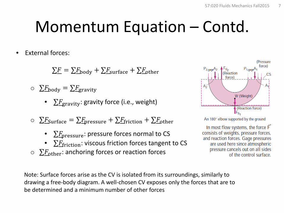
Momentum Equation – Contd.• External forces:

∑𝐹𝐹 = ∑𝐹𝐹body + ∑𝐹𝐹surface + ∑𝐹𝐹other

o ∑𝐹𝐹body = ∑𝐹𝐹gravity

• ∑𝐹𝐹gravity: gravity force (i.e., weight)

o ∑𝐹𝐹Surface = ∑𝐹𝐹pressure + ∑𝐹𝐹friction + ∑𝐹𝐹other

• ∑𝐹𝐹pressure: pressure forces normal to CS• ∑𝐹𝐹friction: viscous friction forces tangent to CS

o ∑𝐹𝐹other: anchoring forces or reaction forces


Note: Surface forces arise as the CV is isolated from its surroundings, similarly to drawing a free-body diagram. A well-chosen CV exposes only the forces that are to be determined and a minimum number of other forces

Example (Bend)57:020 Fluids Mechanics Fall2015 8

Inlet (1):�̇�𝐷1 = 𝛽𝛽𝑉𝑉1𝐴𝐴1𝑢𝑢1 = 𝑉𝑉1𝑣𝑣1 = 0

Outlet (2):�̇�𝐷2 = 𝛽𝛽𝑉𝑉2𝐴𝐴2𝑢𝑢2 = −𝑉𝑉2 cos 45∘𝑣𝑣2 = −𝑉𝑉2 sin 45∘

�̇�𝐷𝑢𝑢 out − �̇�𝐷𝑢𝑢 in = 𝛽𝛽𝑉𝑉2𝐴𝐴2 −𝑉𝑉2 cos 45∘ − 𝛽𝛽𝑉𝑉1𝐴𝐴1 𝑉𝑉1�̇�𝐷𝑣𝑣 out − �̇�𝐷𝑣𝑣 in = 𝛽𝛽𝑉𝑉2𝐴𝐴2 −𝑉𝑉2 sin 45∘ − 𝛽𝛽𝑉𝑉1𝐴𝐴1 0

Since 𝛽𝛽𝑉𝑉1𝐴𝐴1 = 𝛽𝛽𝑉𝑉2𝐴𝐴2,�̇�𝐷𝑢𝑢 out − �̇�𝐷𝑢𝑢 in = − 𝛽𝛽𝑉𝑉2𝐴𝐴2 𝑉𝑉2 cos 45∘ + 𝑉𝑉1�̇�𝐷𝑣𝑣 out − �̇�𝐷𝑣𝑣 in = −𝛽𝛽𝑉𝑉22𝐴𝐴2 sin 45∘

𝑢𝑢2𝑣𝑣2

𝑢𝑢1

This slide contains an example problem and its contents (except for general formula) should NOT be included in your cheat-sheet.

Example – Contd.57:020 Fluids Mechanics Fall2015 9

∑𝐹𝐹𝑥𝑥:1) Body force = 02) Pressure force = 𝑝𝑝1𝐴𝐴1 + 𝑝𝑝2𝐴𝐴2 cos 45∘3) Anchoring force = −𝐹𝐹𝐴𝐴𝑥𝑥

∑𝐹𝐹𝑦𝑦:1) Body force = −𝑊𝑊𝑤𝑤 −𝑊𝑊𝑒𝑒2) Pressure force = 𝑝𝑝2𝐴𝐴2 sin 45∘3) Anchoring force = −𝐹𝐹𝐴𝐴𝑧𝑧

Thus,− 𝛽𝛽𝑉𝑉2𝐴𝐴2 𝑉𝑉2 cos 45∘ + 𝑉𝑉1 = 𝑝𝑝1𝐴𝐴1 + 𝑝𝑝2𝐴𝐴2 cos 45∘ − 𝐹𝐹𝐴𝐴𝑥𝑥−𝛽𝛽𝑉𝑉22𝐴𝐴2 sin 45∘ = −𝛾𝛾𝑉𝑉𝑤𝑤 −𝑊𝑊𝑒𝑒 + 𝑝𝑝2𝐴𝐴2 sin 45∘ − 𝐹𝐹𝐴𝐴𝑧𝑧

∴ 𝐹𝐹𝐴𝐴𝑥𝑥 = 𝛽𝛽𝑉𝑉2𝐴𝐴2 𝑉𝑉2 cos 45∘ + 𝑉𝑉1 + 𝑝𝑝1𝐴𝐴1 + 𝑝𝑝2𝐴𝐴2 cos 45∘𝐹𝐹𝐴𝐴𝑧𝑧 = 𝛽𝛽𝑉𝑉22𝐴𝐴2 sin 45∘ − 𝛾𝛾𝑉𝑉𝑤𝑤 −𝑊𝑊𝑒𝑒 + 𝑝𝑝2𝐴𝐴2 sin 45∘

𝑝𝑝2𝐴𝐴2 cos 45∘𝑝𝑝2𝐴𝐴2 sin 45∘

𝑝𝑝2𝐴𝐴2


Energy Equation• RTT with 𝐵𝐵 = 𝐷𝐷 and 𝛽𝛽 = 𝑒𝑒,

𝜕𝜕𝜕𝜕𝐷𝐷�CV𝑒𝑒𝛽𝛽𝛽𝛽𝑉𝑉 + �

CS𝑒𝑒𝛽𝛽𝑉𝑉 ⋅ 𝛽𝛽𝐴𝐴 = �̇�𝑄 − �̇�𝑊

• Simplified form:

𝑝𝑝in𝛾𝛾 + 𝛼𝛼in

𝑉𝑉in2

2g + 𝑧𝑧in + ℎ𝑝𝑝 =𝑝𝑝out𝛾𝛾 + 𝛼𝛼out

𝑉𝑉out2

2g + 𝑧𝑧out + ℎ𝑡𝑡 + ℎ𝐿𝐿

• 𝑉𝑉 in energy equation refers to average velocity �𝑉𝑉

• 𝛼𝛼 : kinetic energy correction factor = �1 for uniform flow across CS

2 for laminar pipe flow≈ 1 for turbulent pipe flow


Energy Equation - Contd.Uniform flow across CS’s:

𝑝𝑝1𝛾𝛾

+𝑉𝑉12

2g+ 𝑧𝑧1 + ℎ𝑝𝑝 =

𝑝𝑝2𝛾𝛾

+𝑉𝑉22

2g+ 𝑧𝑧1 + ℎ𝑡𝑡 + ℎ𝐿𝐿

• Pump head ℎ𝑝𝑝 = �̇�𝑊𝑝𝑝

�̇�𝑑g= �̇�𝑊𝑝𝑝

𝜌𝜌𝜌𝜌g= �̇�𝑊𝑝𝑝

𝛾𝛾𝜌𝜌⇒ �̇�𝑊𝑝𝑝 = �̇�𝐷gℎ𝑝𝑝 = 𝛽𝛽g𝑄𝑄ℎ𝑝𝑝 = 𝛾𝛾𝑄𝑄ℎ𝑝𝑝

• Turbine head ℎ𝑡𝑡 = �̇�𝑊𝑡𝑡�̇�𝑑g

= �̇�𝑊𝑡𝑡𝜌𝜌𝜌𝜌g

= �̇�𝑊𝑡𝑡𝛾𝛾𝜌𝜌

⇒ �̇�𝑊𝑡𝑡 = �̇�𝐷gℎ𝑡𝑡 = 𝛽𝛽g𝑄𝑄ℎ𝑡𝑡 = 𝛾𝛾𝑄𝑄ℎ𝑡𝑡

• Head loss ℎ𝐿𝐿 = ⁄loss g = ⁄�𝑢𝑢2 − �𝑢𝑢1 g − ⁄�̇�𝑄 �̇�𝐷g > 0


Example (Pump)57:020 Fluids Mechanics Fall2015 12

Energy equation:

𝑝𝑝1𝛾𝛾

+𝑉𝑉12

2g+ 𝑧𝑧1 + ℎ𝑝𝑝 =

𝑝𝑝2𝛾𝛾

+𝑉𝑉22

2g+ 𝑧𝑧2 + ℎ𝑡𝑡 + ℎ𝐿𝐿

With 𝑝𝑝1 = 𝑝𝑝2 = 0, 𝑉𝑉1 = 𝑉𝑉2 ≈ 0, ℎ𝑡𝑡 = 0, and ℎ𝐿𝐿 = 23 m

ℎ𝑝𝑝 = 𝑧𝑧2 − 𝑧𝑧1 + ℎ𝐿𝐿 = 45 + 23 = 68 m

Pump power,

�̇�𝑊𝑝𝑝 = 𝛾𝛾𝑄𝑄ℎ𝑝𝑝 =68 9790 0.03

746 = 80 hp

(Note: 1 hp = 746 N⋅m/s = 550 ft⋅lbf/s)


Differential Analysis57:020 Fluids Mechanics Fall2015 13

A microscopic description of fluid motions for a fluid particle by using differential

equations*,

• Continuity equation

𝜕𝜕𝛽𝛽𝜕𝜕𝐷𝐷 + 𝛻𝛻 ⋅ 𝛽𝛽𝑉𝑉 = 0

• Momentum equation

𝛽𝛽𝜕𝜕𝑉𝑉𝜕𝜕𝐷𝐷 + 𝑉𝑉 ⋅ 𝛻𝛻𝑉𝑉 = 𝛽𝛽g − 𝛻𝛻𝑝𝑝 + 𝛻𝛻 ⋅ 𝜏𝜏𝑖𝑖𝑖𝑖

*CV analysis is a macroscopic description of fluid motions by using integral

equations (RTT).

Navier-Stokes EquationsFor incompressible, Newtonian fluids,

• Continuity:

𝜕𝜕𝑢𝑢𝜕𝜕𝜕𝜕

+𝜕𝜕𝑣𝑣𝜕𝜕𝜕𝜕

+𝜕𝜕𝑤𝑤𝜕𝜕𝑧𝑧

= 0

• Momentum:

𝛽𝛽𝜕𝜕𝑢𝑢𝜕𝜕𝐷𝐷

+ 𝑢𝑢𝜕𝜕𝑢𝑢𝜕𝜕𝜕𝜕

+ 𝑣𝑣𝜕𝜕𝑢𝑢𝜕𝜕𝜕𝜕

+ 𝑤𝑤𝜕𝜕𝑢𝑢𝜕𝜕𝑧𝑧

= −𝜕𝜕𝑝𝑝𝜕𝜕𝜕𝜕

+ 𝛽𝛽g𝑥𝑥 + 𝜇𝜇𝜕𝜕2𝑢𝑢𝜕𝜕𝜕𝜕2

+𝜕𝜕2𝑢𝑢𝜕𝜕𝜕𝜕2

+𝜕𝜕2𝑢𝑢𝜕𝜕𝑧𝑧2

𝛽𝛽𝜕𝜕𝑣𝑣𝜕𝜕𝐷𝐷

+ 𝑢𝑢𝜕𝜕𝑣𝑣𝜕𝜕𝜕𝜕

+ 𝑣𝑣𝜕𝜕𝑣𝑣𝜕𝜕𝜕𝜕

+ 𝑤𝑤𝜕𝜕𝑣𝑣𝜕𝜕𝑧𝑧

= −𝜕𝜕𝑝𝑝𝜕𝜕𝜕𝜕

+ 𝛽𝛽g𝑦𝑦 + 𝜇𝜇𝜕𝜕2𝑣𝑣𝜕𝜕𝜕𝜕2

+𝜕𝜕2𝑣𝑣𝜕𝜕𝜕𝜕2

+𝜕𝜕2𝑣𝑣𝜕𝜕𝑧𝑧2

𝛽𝛽𝜕𝜕𝑤𝑤𝜕𝜕𝐷𝐷

+ 𝑢𝑢𝜕𝜕𝑤𝑤𝜕𝜕𝜕𝜕

+ 𝑣𝑣𝜕𝜕𝑤𝑤𝜕𝜕𝜕𝜕

+ 𝑤𝑤𝜕𝜕𝑤𝑤𝜕𝜕𝑧𝑧

= −𝜕𝜕𝑝𝑝𝜕𝜕𝑧𝑧

+ 𝛽𝛽g𝑧𝑧 + 𝜇𝜇𝜕𝜕2𝑤𝑤𝜕𝜕𝜕𝜕2

+𝜕𝜕2𝑤𝑤𝜕𝜕𝜕𝜕2

+𝜕𝜕2𝑤𝑤𝜕𝜕𝑧𝑧2


Exact Solutions of NS Eqns.The flow of interest is assumed additionally (than incompressible & Newtonian), for example,

1) Steady (i.e., ⁄𝝏𝝏 𝝏𝝏𝝏𝝏 = 𝟎𝟎 for any variable)2) Parallel such that the 𝜕𝜕-component of velocity is zero (i.e., 𝒗𝒗 = 𝟎𝟎)3) Purely two dimensional (i.e., 𝒘𝒘 = 𝟎𝟎 and ⁄𝝏𝝏 𝝏𝝏𝝏𝝏 = 𝟎𝟎 for any velocity

component)4) Fully developed (i.e., ⁄𝝏𝝏 𝝏𝝏𝝏𝝏 = 𝟎𝟎 for any velocity component)

e.g.)

𝛽𝛽�𝜕𝜕𝑢𝑢𝜕𝜕𝐷𝐷

1)

+ 𝑢𝑢�𝜕𝜕𝑢𝑢𝜕𝜕𝜕𝜕

4)

+ ⏞𝑣𝑣2) 𝜕𝜕𝑢𝑢𝜕𝜕𝜕𝜕 +

�𝑤𝑤𝜕𝜕𝑢𝑢𝜕𝜕𝑧𝑧

3)

= −𝜕𝜕𝑝𝑝𝜕𝜕𝜕𝜕 + 𝛽𝛽g𝑥𝑥 + 𝜇𝜇

�𝜕𝜕2𝑢𝑢𝜕𝜕𝜕𝜕2

4)

+𝜕𝜕2𝑢𝑢𝜕𝜕𝜕𝜕2 +

�𝜕𝜕2𝑢𝑢𝜕𝜕𝑧𝑧2

3)

or

𝜇𝜇𝛽𝛽2𝑢𝑢𝛽𝛽𝜕𝜕2 =

𝜕𝜕𝑝𝑝𝜕𝜕𝜕𝜕 − 𝛽𝛽g𝑥𝑥


Boundary ConditionsCommon BC’s:

• No-slip condition (𝑉𝑉fluid = 𝑉𝑉wall; for a stationary wall 𝑉𝑉fluid = 0)

• Interface boundary condition (𝑉𝑉𝐴𝐴 = 𝑉𝑉𝐵𝐵 and 𝜏𝜏𝑠𝑠,𝐴𝐴 = 𝜏𝜏𝑠𝑠,𝐵𝐵)

• Free-surface boundary condition (𝑝𝑝liquid = 𝑝𝑝gas and 𝜏𝜏𝑠𝑠,liquid = 0)

Other BC’s:

• Inlet/outlet boundary condition

• Symmetry boundary condition

• Initial condition (for unsteady flow problem)


Example: No pressure gradient57:020 Fluids Mechanics Fall2015 17

𝜇𝜇𝛽𝛽2𝑢𝑢𝛽𝛽𝜕𝜕2

= 0

Integrate twice,𝑢𝑢 𝜕𝜕 = 𝐶𝐶1𝜕𝜕 + 𝐶𝐶2

B.C.,𝑢𝑢 0 = (𝐶𝐶1) 0 + 𝐶𝐶2 = 0 ⇒ 𝐶𝐶2 = 0

𝑢𝑢 𝑏𝑏 = 𝐶𝐶1 𝑏𝑏 + 𝐶𝐶2 = 𝑈𝑈 ⇒ 𝐶𝐶1 =𝑈𝑈𝑏𝑏

∴ 𝑢𝑢 𝜕𝜕 =𝑈𝑈𝑏𝑏 𝜕𝜕

Analysis:

𝜏𝜏𝑤𝑤 = 𝜇𝜇 �𝛽𝛽𝑢𝑢𝛽𝛽𝜕𝜕 𝑦𝑦=0

= 𝜇𝜇𝑈𝑈𝑏𝑏 =

𝜇𝜇𝑈𝑈𝑏𝑏


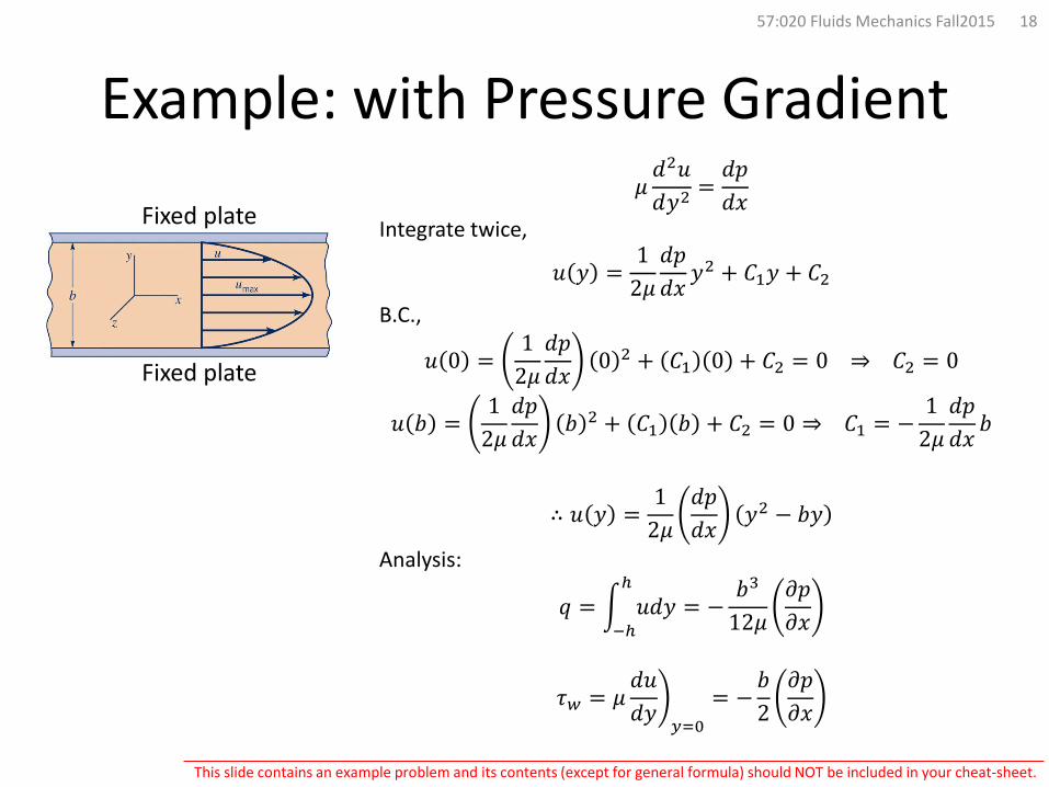
Example: with Pressure Gradient𝜇𝜇𝛽𝛽2𝑢𝑢𝛽𝛽𝜕𝜕2

=𝛽𝛽𝑝𝑝𝛽𝛽𝜕𝜕

Integrate twice,

𝑢𝑢 𝜕𝜕 =12𝜇𝜇

𝛽𝛽𝑝𝑝𝛽𝛽𝜕𝜕

𝜕𝜕2 + 𝐶𝐶1𝜕𝜕 + 𝐶𝐶2B.C.,

𝑢𝑢 0 =12𝜇𝜇


0 2 + 𝐶𝐶1 0 + 𝐶𝐶2 = 0 ⇒ 𝐶𝐶2 = 0

𝑢𝑢 𝑏𝑏 =12𝜇𝜇


𝑏𝑏 2 + 𝐶𝐶1 𝑏𝑏 + 𝐶𝐶2 = 0 ⇒ 𝐶𝐶1 = −12𝜇𝜇


𝑏𝑏

∴ 𝑢𝑢 𝜕𝜕 =12𝜇𝜇


𝜕𝜕2 − 𝑏𝑏𝜕𝜕

Analysis:

𝑞𝑞 = �−ℎ

ℎ𝑢𝑢𝛽𝛽𝜕𝜕 = −

𝑏𝑏3

12𝜇𝜇𝜕𝜕𝑝𝑝𝜕𝜕𝜕𝜕


= −𝑏𝑏2

𝜕𝜕𝑝𝑝𝜕𝜕𝜕𝜕


Fixed plate

Fixed plate


Example: Inclined wall𝜇𝜇𝛽𝛽2𝑢𝑢𝛽𝛽𝜕𝜕2

= −𝛽𝛽g𝑥𝑥Integrate twice,

𝑢𝑢 𝜕𝜕 = −𝛽𝛽g𝑥𝑥2𝜇𝜇

𝜕𝜕2 + 𝐶𝐶1𝜕𝜕 + 𝐶𝐶2B.C.,

𝑢𝑢 0 = −𝛽𝛽g𝑥𝑥𝜇𝜇

0 2 + 𝐶𝐶1 0 + 𝐶𝐶2 = 0 ⇒ 𝐶𝐶2 = 0

�𝛽𝛽𝑢𝑢𝛽𝛽𝜕𝜕 𝑦𝑦=ℎ

= −𝛽𝛽g𝑥𝑥𝜇𝜇

ℎ + 𝐶𝐶1 = 0 ⇒ 𝐶𝐶1 =𝛽𝛽g𝑥𝑥𝜇𝜇

ℎ

∴ 𝑢𝑢 𝜕𝜕 =𝛽𝛽g𝑥𝑥𝜇𝜇

ℎ𝜕𝜕 −𝜕𝜕2

2Analysis:

𝑞𝑞 = �0

ℎ𝑢𝑢𝛽𝛽𝜕𝜕 =

𝛽𝛽g𝑥𝑥𝜇𝜇

ℎ3

3


= 𝜇𝜇𝛽𝛽g𝑥𝑥𝜇𝜇

ℎ = 𝛽𝛽g𝑥𝑥ℎ


Note:g = g𝑥𝑥�̂�𝚤 + g𝑦𝑦 ̂𝚥𝚥

where,g𝑥𝑥 = g sin𝜃𝜃

g𝑦𝑦 = −g cos𝜃𝜃


Buckingham Pi Theorem

• For any physically meaningful equation involving 𝒏𝒏 variables, such as

𝑢𝑢1 = 𝑓𝑓 𝑢𝑢2,𝑢𝑢3,⋯ , 𝑢𝑢𝑛𝑛

with minimum number of 𝒎𝒎 reference dimensions, the equation can be rearranged into product of 𝒓𝒓 dimensionless pi terms.

Π1 = 𝜙𝜙 Π2,Π3,⋯ ,Π𝑟𝑟

where,𝒓𝒓 = 𝒏𝒏 −𝒎𝒎


Similarity and Model TestingIf all relevant dimensionless parameters have the same corresponding values for model and prototype, flow conditions for a model test are completely similar to those for prototype.

For,Π1 = 𝜙𝜙 Π2, … ,Π𝑛𝑛

Similarity requirements:Π2,model = Π2,prototype

⋮Π𝑛𝑛,model = Π𝑛𝑛,prototype

Prediction equation:Π1,model = Π1,prototype


Example (Repeating Variable Method)

Example: The pressure drop per unit length Δ𝑝𝑝ℓ in a pipe flow is a function of the pipe diameter 𝐷𝐷 and the fluid density 𝛽𝛽, viscosity 𝜇𝜇, and velocity 𝑉𝑉.


Δ𝑝𝑝ℓ = 𝑓𝑓 𝐷𝐷,𝛽𝛽, 𝜇𝜇,𝑉𝑉

𝑟𝑟 = 𝑛𝑛 − 𝐷𝐷 = 5 − 3 = 2

Δ𝑝𝑝ℓ 𝐷𝐷 𝛽𝛽 𝜇𝜇 𝑉𝑉

𝑀𝑀𝐿𝐿−2𝑇𝑇−2 𝐿𝐿 𝑀𝑀𝐿𝐿−3 𝑀𝑀𝐿𝐿−1𝑇𝑇−1 𝐿𝐿𝑇𝑇−1


Example – Contd.Select 𝐷𝐷 = 3 repeating variables, 𝐷𝐷,𝑉𝑉,𝛽𝛽 for 𝐿𝐿,𝑇𝑇,𝑀𝑀 , then

Π1 = 𝐷𝐷𝑎𝑎𝑉𝑉𝑏𝑏𝛽𝛽𝑐𝑐Δ𝑝𝑝ℓ =̇ 𝐿𝐿 𝑎𝑎 𝐿𝐿𝑇𝑇−1 𝑏𝑏 𝑀𝑀𝐿𝐿−3 𝑐𝑐 𝑀𝑀𝐿𝐿−2𝑇𝑇−2 =̇ 𝑀𝑀0𝐿𝐿0𝑇𝑇0

𝑎𝑎 + 𝑏𝑏 − 3𝑐𝑐 − 2 = 0−𝑏𝑏 − 2 = 0𝑐𝑐 + 1 = 0

⇒ 𝑎𝑎 = −1, 𝑏𝑏 = −2, 𝑐𝑐 = −1

⇒ Π1 = 𝐷𝐷−1𝑉𝑉−2𝛽𝛽−1Δ𝑝𝑝ℓ =Δ𝑝𝑝ℓ𝐷𝐷𝛽𝛽𝑉𝑉2

Π2 = 𝐷𝐷𝑎𝑎𝑉𝑉𝑏𝑏𝛽𝛽𝑐𝑐𝜇𝜇 =̇ 𝐿𝐿 𝑎𝑎 𝐿𝐿𝑇𝑇−1 𝑏𝑏 𝑀𝑀𝐿𝐿−3 𝑐𝑐 𝑀𝑀𝐿𝐿−1𝑇𝑇−1 =̇ 𝑀𝑀0𝐿𝐿0𝑇𝑇0

𝑎𝑎 + 𝑏𝑏 − 3𝑐𝑐 − 1 = 0−𝑏𝑏 − 1 = 0𝑐𝑐 + 1 = 0

⇒ 𝑎𝑎 = −1, 𝑏𝑏 = −1, 𝑐𝑐 = −1

⇒ Π2 = 𝐷𝐷−1𝑉𝑉−1𝛽𝛽−1𝜇𝜇 =𝜇𝜇

𝐷𝐷𝑉𝑉𝛽𝛽

∴Δ𝑝𝑝ℓ𝐷𝐷𝛽𝛽𝑉𝑉2

= 𝜙𝜙𝛽𝛽𝑉𝑉𝐷𝐷𝜇𝜇



Example (Model Testing)

Δ𝑝𝑝ℓ𝐷𝐷𝛽𝛽𝑉𝑉2 = 𝜙𝜙

𝛽𝛽𝑉𝑉𝐷𝐷𝜇𝜇


Model Prototype

If,𝛽𝛽𝑑𝑑𝑉𝑉𝑑𝑑𝐷𝐷𝑑𝑑𝜇𝜇𝑑𝑑

=𝛽𝛽𝑝𝑝𝑉𝑉𝑝𝑝𝐷𝐷𝑝𝑝𝜇𝜇𝑝𝑝

similarity requirement

Then,Δ𝑝𝑝ℓ𝑑𝑑𝐷𝐷𝑑𝑑𝛽𝛽𝑑𝑑𝑉𝑉𝑑𝑑2

=Δ𝑝𝑝ℓ𝑝𝑝𝐷𝐷𝑝𝑝𝛽𝛽𝑝𝑝𝑉𝑉𝑝𝑝2

(Prediction equation)


Example – Contd.57:020 Fluids Mechanics Fall2015 25

Model (in water)• 𝐷𝐷𝑑𝑑 = 0.1 m• 𝛽𝛽𝑑𝑑 = 998 kg/m3

• 𝜇𝜇𝑑𝑑 = 1.12 × 10-3 N⋅s/m2

• 𝑉𝑉𝑑𝑑 = ?• Δ𝑝𝑝ℓ𝑑𝑑 = 27.6 Pa/m

Prototype (in air)• 𝐷𝐷𝑝𝑝 = 1 m• 𝛽𝛽𝑝𝑝 = 1.23 kg/m3

• 𝜇𝜇𝑝𝑝 = 1.79 × 10-5 N⋅s/m2

• 𝑉𝑉𝑝𝑝 = 10 m/s• Δ𝑝𝑝ℓ𝑑𝑑 = ?

Similarity requirement:

𝑉𝑉𝑑𝑑 =𝛽𝛽𝑝𝑝𝛽𝛽𝑑𝑑

𝜇𝜇𝑑𝑑𝜇𝜇𝑝𝑝

𝐷𝐷𝑝𝑝𝐷𝐷𝑑𝑑

𝑉𝑉𝑝𝑝 =1.23998

1.12 × 10−3

1.79 × 10−51

0.1 10 = 𝟕𝟕.𝟕𝟕𝟕𝟕 ⁄𝐦𝐦 𝐬𝐬

Prediction equation:

Δ𝑝𝑝ℓ𝑝𝑝 =𝐷𝐷𝑑𝑑𝐷𝐷𝑝𝑝

𝛽𝛽𝑝𝑝𝛽𝛽𝑑𝑑

𝑉𝑉𝑝𝑝𝑉𝑉𝑑𝑑

2

Δ𝑝𝑝ℓ𝑑𝑑 =0.11

1.23998

107.71

2

27.6 = 𝟓𝟓.𝟕𝟕𝟕𝟕 × 𝟕𝟕𝟎𝟎−𝟑𝟑 ⁄𝐏𝐏𝐏𝐏 𝐦𝐦


Pipe Flow: Laminar vs. Turbulent

• Reynolds number regimes

Re =𝛽𝛽𝑉𝑉𝐷𝐷𝜇𝜇

26

Re < Recrit ∼ 2,000

Recrit < Re < Retrans

Re > 𝑅𝑅𝑒𝑒trans ∼ 4,000

57:020 Fluids Mechanics Fall2015

Flow in Pipes

• Basic piping problems:– Given the desired flow rate, what pressure drop (e.g.,

pump power) is needed to drive the flow (i.e., to overcome the head loss through piping)?

– Given the pressure drop (e.g., pump power) available, what flow rate will ensue?

– Given the pressure drop and the flow rate desired, what pipe diameter is needed?


Head Lossℎ𝐿𝐿 = ℎ𝐿𝐿major + ℎ𝐿𝐿 minor

• ℎ𝐿𝐿 major (or ℎ𝑓𝑓): Major loss, the loss due to viscous effects• ℎ𝐿𝐿 minor: Minor loss, the loss in the various pipe components

Darcy-Weisbach equation

ℎ𝑓𝑓 = 𝑓𝑓𝐿𝐿𝐷𝐷𝑉𝑉2

2g

• 𝑓𝑓 = 8𝜏𝜏𝑤𝑤𝜌𝜌𝑉𝑉2

: Friction factor

• 𝐿𝐿: Pipe length• 𝐷𝐷: Pipe diameter• 𝑉𝑉: Average flow velocity across the pipe cross-section


Laminar Pipe Flow• Exact solution exists by solving the NS equation

𝑢𝑢 𝑟𝑟 = 𝑉𝑉max 1 −𝑟𝑟𝑅𝑅

2, 𝑉𝑉max = 2𝑉𝑉

• Wall shear stress

𝜏𝜏𝑤𝑤 = −𝜇𝜇 �𝛽𝛽𝑢𝑢𝛽𝛽𝑟𝑟 𝑟𝑟=𝑅𝑅

=8𝜇𝜇𝑉𝑉𝐷𝐷

• Friction factor

𝑓𝑓 =8𝜏𝜏𝑤𝑤𝛽𝛽𝑉𝑉2

=64𝜇𝜇𝛽𝛽𝐷𝐷𝑉𝑉

=64Re

• Head loss


2g=32𝜇𝜇𝐿𝐿𝑉𝑉𝛾𝛾𝐷𝐷2

=128𝜇𝜇𝐿𝐿𝑄𝑄𝜋𝜋𝛾𝛾𝐷𝐷4


Notes: 𝑄𝑄 = 𝑉𝑉𝐴𝐴

𝐴𝐴 =𝜋𝜋𝐷𝐷2

4

Turbulent Pipe Flow• From a dimensional analysis

𝑓𝑓 = 𝜙𝜙 Re, ⁄𝜀𝜀 𝐷𝐷

• Moody chart: Empirical functional dependency of 𝑓𝑓 on Re and ⁄𝜀𝜀 𝐷𝐷


Turbulent Pipe Flow – Cond.• Colebrook equation (difficult in its use as implicit)

1𝑓𝑓

= −2 log⁄𝜀𝜀 𝐷𝐷

3.7+

2.51𝑅𝑅𝑒𝑒 𝑓𝑓

• Haaland equation (easier to use as explicit but approximation)

1𝑓𝑓

= −1.8 log⁄𝜀𝜀 𝐷𝐷

3.7

1.1

+6.9𝑅𝑅𝑒𝑒


Example (pipe flow)3257:020 Fluids Mechanics Fall2015

Energy equation:𝑝𝑝1𝛾𝛾 + 𝛼𝛼1

𝑉𝑉12

2g + 𝑧𝑧1 =𝑝𝑝2𝛾𝛾 + 𝛼𝛼2

𝑉𝑉22

2g + 𝑧𝑧2 + ℎ𝑓𝑓Since 𝑝𝑝1 = 𝑝𝑝2 = 0 and 𝑉𝑉1 = 𝑉𝑉2,

ℎ𝑓𝑓 = 𝑧𝑧1 − 𝑧𝑧2 = Δ𝑧𝑧Friction factor,

1𝑓𝑓

= −1.8 log0.00033

3.7

1.1

+6.9

1.75 × 106 ⇒ 𝑓𝑓 = 0.0159

Head loss


2g = 0.0159(1700)

(1.5)14.1 2

2 (32.2) = 56 ft

∴ Δ𝑧𝑧 = 𝟓𝟓𝟓𝟓 𝐟𝐟𝐟𝐟

If D = 1.5 ft and Q = 25 ft3/s, ∆z = z1 – z2? Neglect minor losses.

𝑉𝑉 =𝑄𝑄𝐴𝐴 =

25⁄𝜋𝜋 1.5 2 4 = 14.1 ⁄ft s

Re =𝑉𝑉𝐷𝐷𝜈𝜈 =

(14.1)(1.5)1.21 × 10−5 = 1.75 × 106 (turbulent)

⁄𝜀𝜀 𝐷𝐷 = ⁄0.0005 1.63 = 0.00033


Review for Exam2 - University of Iowafluids/Posting/Exams... · 2015-11-13 · Review for Exam2 11....

Documents

Transcript of Review for Exam2 - University of Iowafluids/Posting/Exams... · 2015-11-13 · Review for Exam2 11....