Rev. 03 STP 3 & 4 Environmental Report
70
Water 2.3-1 STP 3 & 4 Environmental Report 2.3 Water This section describes the hydrology, water use, and water quality characteristics of the STP site and surrounding region that could affect or be affected by the construction and operation of two Advanced Boiling Water Reactor (ABWR) units, which will be referred to as STP 3 & 4. The potential water-related impacts of construction and operation are discussed in Chapters 4 and 5, respectively. The STP site is located in Matagorda County, Texas, near the west bank of the Colorado River, opposite river mile 14.6. It is approximately 12 miles south-southwest of Bay City, Texas, and 8 miles north-northwest of Matagorda, Texas (Figure 2.3.1-1). The surface elevation of the site ranges from approximately 32 to 34 ft above mean sea level (MSL) at the north boundary to between 15 ft and 20 ft MSL at the south end. The existing grade at the location for STP 3 & 4 is approximately 30 ft MSL and the finish plant grade in the STP 3 & 4 power block area is anticipated to be between 32 ft and 36.5 ft MSL. 2.3.1 Hydrology This section describes surface water bodies and groundwater aquifers that could affect the plant water supply and effluent disposal or that could be affected by the construction and operation of STP 3 & 4. The site-specific and regional data on the physical and hydrologic characteristics of these water resources are summarized in the following sections. 2.3.1.1 Surface Water 2.3.1.1.1 The Colorado River Basin The Colorado River Basin extends across the middle of Texas, from the southeastern portion of New Mexico to Matagorda Bay at the Gulf of Mexico. The total drainage area of the Colorado River is 42,318 mi 2 , of which 11,403 mi 2 are considered non- contributory to the river’s water supply (Reference 2.3.1-1). The Lower Colorado River Basin is the part of the river system from Lake O.H. Ivie to the Gulf Coast (Figure 2.3.1-2) and comprises approximately 22,682 mi 2 of drainage area (Reference 2.3.1- 2). The Upper Colorado River Basin has a drainage area of approximately 19,636 mi 2 . There are six major tributaries with drainage areas greater than 900 mi 2 that contribute to the Colorado River: Beals Creek and the Concho River in the Upper Colorado River Basin and the San Saba, Llano, Pedernales Rivers and Pecan Bayou in the Lower Colorado River Basin. These major tributaries, and approximately 90% of the entire contributing drainage for the river, occur upstream of Mansfield Dam near Austin. Downstream of Austin, there are only two tributaries with drainage areas greater than 200 mi 2 , Barton Creek and Onion Creek in Travis County (Reference 2.3.1-1). Table 2.3.1-1 summarizes the drainage areas of major freshwater streams in the Colorado River Basin. The Colorado River Basin lies in the warm-temperate/subtropical zone, and its subtropical climate is typified by dry winters and humid summers. Spring and fall are both wet seasons in this region with rainfall peaks in May and September. The spring Rev. 03
Transcript of Rev. 03 STP 3 & 4 Environmental Report
STP 3 & 4 Environmental Report
Rev. 03
2.3 WaterThis section describes the hydrology, water use, and water quality characteristics of the STP site and surrounding region that could affect or be affected by the construction and operation of two Advanced Boiling Water Reactor (ABWR) units, which will be referred to as STP 3 & 4. The potential water-related impacts of construction and operation are discussed in Chapters 4 and 5, respectively.
The STP site is located in Matagorda County, Texas, near the west bank of the Colorado River, opposite river mile 14.6. It is approximately 12 miles south-southwest of Bay City, Texas, and 8 miles north-northwest of Matagorda, Texas (Figure 2.3.1-1). The surface elevation of the site ranges from approximately 32 to 34 ft above mean sea level (MSL) at the north boundary to between 15 ft and 20 ft MSL at the south end. The existing grade at the location for STP 3 & 4 is approximately 30 ft MSL and the finish plant grade in the STP 3 & 4 power block area is anticipated to be between 32 ft and 36.5 ft MSL.
2.3.1 HydrologyThis section describes surface water bodies and groundwater aquifers that could affect the plant water supply and effluent disposal or that could be affected by the construction and operation of STP 3 & 4. The site-specific and regional data on the physical and hydrologic characteristics of these water resources are summarized in the following sections.
2.3.1.1 Surface Water
2.3.1.1.1 The Colorado River Basin The Colorado River Basin extends across the middle of Texas, from the southeastern portion of New Mexico to Matagorda Bay at the Gulf of Mexico. The total drainage area of the Colorado River is 42,318 mi2, of which 11,403 mi2 are considered non-contributory to the river’s water supply (Reference 2.3.1-1). The Lower Colorado River Basin is the part of the river system from Lake O.H. Ivie to the Gulf Coast (Figure2.3.1-2) and comprises approximately 22,682 mi2 of drainage area (Reference 2.3.1-2). The Upper Colorado River Basin has a drainage area of approximately 19,636 mi2. There are six major tributaries with drainage areas greater than 900 mi2 that contribute to the Colorado River: Beals Creek and the Concho River in the Upper Colorado River Basin and the San Saba, Llano, Pedernales Rivers and Pecan Bayou in the Lower Colorado River Basin. These major tributaries, and approximately 90% of the entire contributing drainage for the river, occur upstream of Mansfield Dam near Austin. Downstream of Austin, there are only two tributaries with drainage areas greater than 200 mi2, Barton Creek and Onion Creek in Travis County (Reference 2.3.1-1). Table 2.3.1-1 summarizes the drainage areas of major freshwater streams in the Colorado River Basin.
The Colorado River Basin lies in the warm-temperate/subtropical zone, and its subtropical climate is typified by dry winters and humid summers. Spring and fall are both wet seasons in this region with rainfall peaks in May and September. The spring
Water 2.3-1
STP 3 & 4 Environmental Report
Rev. 03
rains are produced by convective thunderstorms, which result in high intensity, short duration precipitation events with rapid runoff. The fall rains are primarily governed by tropical storms and hurricanes that originate in the Caribbean Sea or the Gulf of Mexico. These rains pose flooding risks to the Gulf Coast from Louisiana to Mexico. The spatial rainfall distribution in this region varies from an annual amount of 44 inches at the coast to 24 inches in the northwestern portion of the region (Reference 2.3.1-1). The Colorado River Basin is located in a semi-arid region, and its hydrologic characteristics are closely linked to the weather in this area, which has been described as a “continuous drought periodically interrupted by floods” (Reference 2.3.1-3).
Stream flow gauging data collected in the Colorado River since the early 1900s show that there has been a major drought in almost every decade of the twentieth century, with severe droughts occurring every 20 to 40 years. Major droughts in the basin cause stock ponds and small reservoirs to go dry and large reservoirs, such as Lake Travis, to significantly drop their storage levels, to as much as one third of their storage capacity. During the 30-year time period from 1941 to 1970, there were three major statewide droughts; from 1947 to 1948, from 1950 to 1957, and from 1960 to 1967. The most severe of these droughts occurred from 1950 to 1957, when 94% of the counties in the state were declared disaster areas (Reference 2.3.1-1).
A drought cycle is often followed by one or more flooding events. Due to very limited vegetative cover, rocky terrain, and steep channels, runoff in the Upper Colorado River Basin is high and rapid, producing fast moving and high-peak floods. The terrain in the Lower Colorado River Basin is flatter with greater vegetative cover and wider floodplains, which reduces the velocity of floods. The Hill Country watershed of the Lower Colorado River has been characterized as “Flash Flood Alley,” meaning that the Lower Colorado River Basin is one of the regions that are most prone to flash flood damage. The susceptibility to flash flooding occurs because the thin soils and steep slopes in the Upper Colorado River Basin promote rapid runoff from the watershed during heavy rain events. Also, the large drainage area of the Hill Country watershed can contribute runoff from hundreds of miles away, transforming heavy rains into flood waters with destructive potential. More than 80 floods have been recorded in this region since the mid-1800s. During these events, water levels exceed the river flood stage and inundate dry lands. The most intense localized flash flood in the Lower Colorado region in recent history occurred in May 1981 in Austin (Reference 2.3.1-1).
Major reservoirs in the Colorado River Basin are summarized in Table 2.3.1-2 (Reference 2.3.1-4 sorted in order of descending storage capacity. The locations of some major dams are shown in Figure 2.3.1-3. Because of the high risk of flooding in the Lower Colorado River Basin, a system of dams and reservoirs has been developed along the river primarily to manage floodwaters, and to conserve and convey water supplies. The Lower Colorado River Authority (LCRA) operates six dams on the Lower Colorado River: Buchanan, Roy Inks, Alvin Wirtz, Max Starcke, Mansfield, and Tom Miller (Figure 2.3.1-4). These dams form the six Highland Lakes; Buchanan, Inks, LBJ, Marble Falls, Travis, and Austin (Reference 2.3.1-5).
2.3.1-2 Hydrology
STP 3 & 4 Environmental Report
Rev. 03
Approximately 28 miles upstream from Austin is Mansfield Dam, which forms Lake Travis, the largest reservoir on the Colorado River. Mansfield Dam is the most downstream existing major control structure on the Colorado River. With the completion of the Simon Freese Dam in 1989, normal flows and flood flows in the Colorado River upstream of Mansfield Dam are regulated by a total of 27 major reservoirs, which includes Lake Travis, with Mansfield Dam providing most of the floodwater storage capacity and precludes short-duration flow fluctuation downstream.
The storage capacities of the remaining upstream reservoirs are relatively small compared to Lake Travis and Lake Buchanan formed by the Buchanan Dam, and are of lesser importance to flood control. Tom Miller Dam at Austin, downstream of Lake Travis, impounds a portion of the Colorado River known as Lake Austin, but because of the small storage capacity of its reservoir, it affords no major control of flood flows.
Lake Travis and Lake Buchanan also serve as water supply reservoirs. With a combined capacity of approximately 4.2 million acre-feet, they store water for communities, industry, and aquatic life along the river, and they supply irrigation water for the agricultural industry near the Gulf Coast.
The Lower Colorado River near the STP site has a relatively shallow gradient and broad floodplain. The average gradient of the river downstream of Austin varies from 1.0 ft/mile to 2.1 ft/mile. The main channel of the Colorado River has the capacity to contain flows ranging from a 6-year to a 21-year return interval from Austin to the Gulf of Mexico. Thus, in any given year there is a 5 to 16% chance that river flows will encroach upon the floodplains. The Lower Colorado River floodplain below Columbus varies from 4 to 8 miles in width with side slopes averaging between 0.009% and 0.028%. In this area, no discernible valley exists, and the floodwaters can spill over beyond the basin divide causing interbasin spillage. As mentioned above, the susceptibility of the Lower Colorado River area to the flash flooding results from regional weather patterns and its geographic proximity to the Gulf of Mexico, which induces very high intensity rainfalls frequently in the summer. Historically, the most severe floods often occurred in May to September as a result of high rainfall intensities (Reference 2.3.1-3), and the area of floodplain extends correspondingly. As the dry season approaches, some floodplains will shrink or even dry up completely.
Table 2.3.1-3 presents pertinent data for seven U.S. Geological Survey (USGS) maintained stream-flow gauge stations downstream of the Mansfield Dam, including location, drainage area, mean, maximum, and minimum average annual flow for the period of record. The locations of these gauges are shown on Figure 2.3.1-5 (Reference 2.3.1-6). The Bay City streamflow gauging station (Gauge 08162500) is the nearest to the STP site, being located approximately 16 miles upstream of the STP site, approximately 2.8 miles west of Bay City, at river mile 32.5 on the Colorado River. Records of water elevation at this station have been collected since the gauge was installed in April 1948. Based on the historical data for the water years 1948 to 2004, the maximum annual average stream flow at this station is 14,270 cubic feet per second (cfs), the minimum annual average flow is 375 cfs, and the mean annual average flow is approximately 2628 cfs.
Hydrology 2.3.1-3
STP 3 & 4 Environmental Report
Rev. 03
In order to facilitate the evaluation of the water supply characteristics at the STP site, a number of flow data statistics are presented for the Colorado River at Bay City. Table 2.3.1-4 presents the mean daily flow rate for each day of the May 1948 to September 2006 period of record (Reference 2.3.1-7). Table 2.3.1-5 presents the mean monthly flow rate for the same period of record (Reference 2.3.1-7). Table 2.3.1-6 gives the minimum daily flow and Table 2.3.1-7 gives the maximum daily flow for each month of the period of record.
Table 2.3.1-8 presents the flood frequency distribution for the Colorado River at Wharton for regulated conditions estimated in Reference 2.3.1-8, Chapter 4: “The basis for the regulated peak discharge frequency curves are the regulated daily flows for the period of record generated by a reservoir system regulation model that takes into account the current system of reservoirs, conservation pool demands and the flood control regulation rules” (Reference 2.3.1-9, Chapter 2, page 1).
Table 2.3.1-9 presents the minimum daily flow at Bay City for the years 1948 to 2006. Table 2.3.1-10 presents the 7-day minimum flow for the same period based on data from Reference 2.3.1-10. The minimum 7-day flow for the period 1948 to 2006 is approximately 0.5 cfs. The minimum daily and minimum 7-day low flows for the years 1948-2006 are also shown in Figure 2.3.1-6. Plotting the low flow data using the Weibull plotting position formula on normal distribution paper and fitting a straight line through the data, the 7-day low flow with a 10-year return period was estimated to be 4.3 cfs.
2.3.1.1.2 Local Hydrologic Features A major feature of the site is the Main Cooling Reservoir (MCR), which is formed by a 12.4-mile-long earthfill embankment constructed above the natural ground surface. The MCR was developed solely for the industrial use of dissipating heat from STP units as an engineered cooling pond. The MCR has a surface area of 7000 acres with a normal maximum operating level of El. 49 ft MSL (Reference 2.3.1-9). The MCR makeup water is withdrawn from the Colorado River adjacent to the site, and provides reservoir storage to account for dry periods during the year. A smaller separate cooling pond, referred to as the Essential Cooling Pond (ECP), serves as the Ultimate Heat Sink (UHS) for STP 1 & 2. The surface area of the ECP is 46 acres.
The MCR was originally sized for four nuclear units similar in size to the existing two units. Therefore, there will be no significant changes to the existing MCR due to the construction of new units, except the addition, on the north dike, of the STP 3 & 4 Circulating Water (CW) pump intake and the STP 3 & 4 outfall west of the existing STP 1 & 2 outfall. To maintain sufficient MCR water inventory to offset evaporation, seepage and blowdown, STP is entitled to divert 55% of the river flow in excess of 300 cfs at the Reservoir Makeup Pumping Facility (RMPF) as MCR makeup, with the annual flow diversion in any given year limited to 102,000 acre-ft (Reference 2.3.1-11). In the event of a repeat of the Lower Colorado River’s Drought of Record (DOR) from 1947 to 1957, the LCRA would be required, by contract, to make available an additional 40,000 acre-ft per year of firm water. This firm water will be made available, without restriction on river flow, for MCR makeup when the water level in MCR is below 35 ft MSL. These arrangements are expected to be adequate to maintain sufficient
2.3.1-4 Hydrology
STP 3 & 4 Environmental Report
Rev. 03
water in the MCR for continuous operation of all four units. This assessment is also supported by the water management plan for the Lower Colorado River (Reference 2.3.1-12).
A significant hydrologic feature near the STP site is Little Robbins Slough. It is an intermittent stream located 9 miles northwest of Matagorda in southwestern Matagorda County and runs south for 6.5 miles to the point where it joins Robbins Slough, a brackish marsh, which meanders for four more miles to the Gulf Intracoastal Waterway (GIWW). During the construction of the MCR for STP 1 & 2, the water course of Little Robbins Slough within the boundary of the STP site was relocated to a channel on the west side of the west embankment of the reservoir, and rejoined its natural course approximately one mile east of the southwest corner of the MCR.
The Design-Basis Flood (DBF) for STP 3 & 4 is based on the potential breach of the dike containing the MCR. The DBF elevation is 48.540.0 ft MSL.
2.3.1.1.3 Adjacent Drainage Basins To the west of the Lower Colorado River Basin is the Colorado-Lavaca River Basin, shown on Figure 2.3.1-7. This basin includes the Tres Palacios River, which is not tributary to either of those rivers. The Colorado-Lavaca River Basin drains into Tres Palacios Bay, northwest of Matagorda Bay. In the event of inter-basin spillage, flood waters from the Colorado River Basin flow into Caney Creek near Wharton, as in the case of the 1913 flood, into the San Bernard Coastal Basin on the east edge of the Colorado River Basin, or into the Colorado-Lavaca River Basin to the west.
2.3.1.1.4 Wetlands The STP site is located in the mid-coast region of the Gulf-Atlantic Coastal Flats, which are characterized by large bay and estuary systems supplied by freshwater inflow from rivers and covered with extensive coastal prairies inland (Figure 2.3.1-8, Reference 2.3.1-13). A study conducted by the Texas General Land Office determined that wetlands and aquatic habitats on Matagorda Island, Matagorda Peninsula, and Colorado River delta are dominated by estuarine emergent wetlands (salt and brackish marshes), which represent 67% of the vegetated wetland and aquatic classes in this area (Reference 2.3.1-14). Among other mapped classes, seagrass beds are most abundant, followed by tidal flats, Gulf beaches, palustrine marshes, and mangroves.
Wetlands in the vicinity of the STP site are mainly associated with the Colorado River and its tributaries. Wetlands within a 6 mile radius of the site are delineated on Figure 2.3.1-9. Wetland inventory data was provided by the U.S. Fish and Wildlife Service (Reference 2.3.1-15). Freshwater emergent wetlands have been identified as the predominant class in this region, encompassing an area of approximately 262 acres in a 6-mile radius from the STP site. Other wetland types found in this region include freshwater forested/shrub wetland and freshwater pond, which cover areas of 13 acres and 1 acre, respectively in the same radius from the site (See Section 2.4). Because wetlands near the site are primarily classified as freshwater types, the area of wetlands covered by water generally reduces in the dry season and expands in the wet season.
Hydrology 2.3.1-5
STP 3 & 4 Environmental Report
Rev. 03
2.3.1.1.5 Erosion and SedimentationMost of the sediment data for the Colorado River have been collected from two USGS daily suspended sediment stations; one near San Saba at river mile 474.3 and the other at the eastern edge of Columbus at river mile 135.1. Because the Columbus gauging station is the closest to the STP site, its sediment records were examined to characterize the suspended sediment loads for the Colorado River. Figure 2.3.1-10 shows in histogram form the annual sediment load based on data collected at this station from March 1957 to September 1973 (Reference 2.3.1-16). Each bar of the histogram is divided into the suspended load discharged in 1% of the year (3.65 days), 10% of the year (36.5 days), and the rest of the year. These frequencies are generated by ranking the sediment load for each day of the year. The data summarized in Figure 2.3.1-10 indicate that the annual sediment load at the Columbus gauging station has declined over time. This decline is likely associated with the creation of impoundments over the same period, which serve as sediment traps in the Colorado River Basin. The data also indicate that major fractions (80-90%) of the total sediment load in individual years are produced by infrequent large storms.
No bed load sediment transport measurements have been reported for any reach of the Colorado River and cannot be easily estimated as a fraction of the suspended load because the portion of sediment that moves as bed load varies widely between rivers and on the same river over time (Reference 2.3.1-17). However, to get an order of magnitude estimate, the globally averaged ratio of suspended load to bed load sediment flux for rivers of 9:1, reported in Reference 2.3.1-18 can be used.
2.3.1.1.6 Shore RegionsThe STP site is located 10.5 miles inland from Matagorda Bay and 16.9 miles inland from the Gulf of Mexico. It is approximately 75 miles from the Continental Shelf. The shoreline of Matagorda Peninsula along the Gulf of Mexico changes constantly, retreating landward or advancing seaward as the result of a combination of hydrologic and meteorological processes, climatic factors as well as engineering activities.
Matagorda Peninsula is a classic microtidal, wave-dominated coast with a mean diurnal tide range of approximately 2.1 ft. An evaluation of 20 years of data shows that the mean significant wave height near the Colorado River entrance is approximately 3.3 ft, with a variation of 1.3 ft during the year (Reference 2.3.1-19). This shore region is also greatly affected by waves generated by tropical storms and hurricanes.
The hydrologic features of the shore region are also altered by a series of engineering interventions. After the removal of a log jam on the Colorado River in 1929, a channel was dredged across the Matagorda Peninsula to allow the river to directly discharge to the Gulf of Mexico in 1936. In the 1990s, the U.S. Army Corps of Engineers (USACE) constructed jetties on each side of the river entrance and dredged an entrance channel. In 1993, USACE constructed a diversion channel that directs the flow of the Colorado River into East Matagorda Bay. The former river channel is now a navigation channel connected to the GIWW.
2.3.1-6 Hydrology
STP 3 & 4 Environmental Report
Rev. 03
Studies conducted recently to calculate the average annual rate of shoreline changes show that the shoreline segment of Matagorda Peninsula 1.6 miles southwest of the Colorado River is retreating at a rate of 1.6 to 6.4 ft/yr (Reference 2.3.1-19). Up north toward the mouth of the Colorado River, the shoreline displays long-term advance, which is related to the sediment supplies from the river, sand bypassing across the entrance jetties, and wave sheltering by the jetties (Reference 2.3.1-19). The shoreline northeast of the Colorado River is relatively stable and shows slight long-term advance in an area 8 miles to the northeast of the river mouth (Reference 2.3.1-19).
2.3.1.1.7 Hydrologic Characteristics of the Intake Structure AreaSTP 3 & 4 will use the MCR for normal plant cooling. The Colorado River is the source of water to make up water losses in the MCR due to evaporation and seepage. For this purpose, STP 3 & 4 will use the existing RMPF on the Colorado River.
Makeup water demands are described in Section 3.3, while the RMPF is discussed in Section 3.4. Based on the dimensions of the RMPF, the total length of the intake is 406 ft, and the depth below normal water surface elevation in front of the intake is 10 ft. The Figure 2.3.1-11 shows a cross section of the Colorado River channel near the RMPF. As can be seen in the figure, the bottom of the river channel is at elevation approximately -14 ft NAVD88. NAVD 88, North America Vertical Datum 88, is the new vertical (elevation) reference system adopted in North America. It is adjusted based on field work prior to 1929 as well as surveys as recent as 1988. Based on the makeup demands described in Section 3.3 and dimensions of the intake presented in Section 3.4, the average water velocity in front of the intake for maximum flow conditions (1200 cfs) would be approximately 0.3 ft/s considering a cross section of approximately 4060 ft2.
2.3.1.2 Groundwater ResourcesThe regional and site-specific data on the physical and hydrologic characteristics of the groundwater resources are summarized in this section to provide the basic data for an evaluation of impacts on the aquifers of the area.
The STP site covers an area of approximately 12,220 acres and is located on the coastal plain of southeastern Texas in Matagorda County (Reference 2.3.1-9). The STP site lies approximately 10 mi north of Matagorda Bay. Nearby communities include Palacios, approximately 10 mi to the southwest, and Bay City, approximately 12 mi to the northeast (Figure 2.3.1-12). The closest major metropolitan center is Houston, approximately 90 mi to the northeast.
The 7000-acre MCR is the predominant feature at the STP site, as shown in Figure 2.3.1-13. The MCR is fully enclosed with a compacted earth embankment and encompasses most of the southern and central portions of the site. The existing STP 1 & 2 facilities are located just outside of the MCR northern embankment. Further north of the embankment and to the northwest of STP 1 & 2 is the proposed area for STP 3 & 4.
Hydrology 2.3.1-7
STP 3 & 4 Environmental Report
Rev. 03
The STP site, in general, has less than 15 ft of natural relief in the 4.5 mi distance from the northern to southern boundary. The northern section is at an elevation of approximately 30 ft MSL. The southeastern section is at an elevation of approximately 15 ft above MSL. The Colorado River flows along the southeastern site boundary. There are also several unnamed drainages in the site boundaries, one of which feeds Kelly Lake.
2.3.1.2.1 Hydrogeologic SettingThe STP site lies in the Gulf Coastal Plains physiographic province in the Coastal Prairies sub-province, which extends as a broad band parallel to the Texas Gulf Coast, as shown in Figure 2.3.1-14 (Reference 2.3.1-20). The Coastal Prairies sub-province is characterized by relatively flat topography with land elevation ranging from sea level along the coast to 300 ft above sea level along the northern and western boundaries. The geologic materials underlying the Coastal Prairies sub-province consist of deltaic deposits.
The STP site is underlain by a thick wedge of southeasterly dipping, sedimentary deposits of Holocene through Oligocene age. The site overlies what has been referred to as the Coastal Lowlands Aquifer System (Figure 2.3.1-15). This aquifer system contains numerous local aquifers in a thick sequence of mostly unconsolidated Coastal Plain sediments of alternating and interfingering beds of clay, silt, sand, and gravel. The sediments reach thicknesses of thousands of feet and contain groundwater that ranges from fresh to saline. Large amounts of groundwater are withdrawn from the aquifer system for municipal, industrial, and irrigation needs (Reference 2.3.1-21).
The lithology of the aquifer system reflects three depositional environments: continental (alluvial plain), transitional (delta, lagoon, and beach), and marine (continental shelf). The depositional basin thickens towards the Gulf of Mexico, resulting in a wedge-shaped configuration of hydrogeologic units. Numerous oscillations of ancient shorelines resulted in a complex, overlapping mixture of sand, silt, and clay (Reference 2.3.1-21).
As part of the USGS Regional Aquifer-System Analysis (RASA) program, the Coastal Lowlands Aquifer System was subdivided into five permeable zones and two confining units. The term “Gulf Coast Aquifer” is generally used in Texas to describe the Coastal Lowlands Aquifer System. A comparison of the USGS aquifer system nomenclature to that used in Texas is shown in Figure 2.3.1-16. A cross-sectional representation is shown in Figure 2.3.1-17 (Reference 2.3.1-21).
The Texas nomenclature is used to describe the Gulf Coast Aquifer beneath the site. The hydrogeologic units commonly used to describe the aquifer system (from shallow to deep) are as follows (Figure 2.3.1-16):
Chicot Aquifer
Evangeline Aquifer
Burkeville Confining Unit
2.3.1-8 Hydrology
STP 3 & 4 Environmental Report
Rev. 03
Jasper Aquifer
Catahoula Confining Unit (restricted to where present in the Jasper Aquifer)
Vicksburg-Jackson Confining Unit
The base of the Gulf Coast Aquifer is identified as either its contact with the top of the Vicksburg-Jackson Confining Unit or the approximate depth where groundwater has a total dissolved solids concentration of more than 10,000 milligrams per liter (mg/l). The aquifer system is recharged by the infiltration of precipitation that falls on aquifer outcrop areas in the northern and western portion of the province. Discharge occurs by evapotranspiration, loss of water to streams and rivers as base flow, upward leakage to shallow aquifers in low lying coastal areas or to the Gulf of Mexico, and pumping.
With the exception of the shallow zones in the vicinity of the outcrops, the water in the Gulf Coast Aquifer is under confined conditions. In the shallow zones, the specific yield for sandy deposits generally ranges between 10 and 30%. For the confined aquifer, the storage coefficient is estimated to range between 1 x 10⁻⁴ and 1 x 10⁻³. The productivity of the aquifer system is directly related to the thickness of the sands in the aquifer system that contain freshwater. The aggregated sand thickness ranges from 0 ft at the up dip limit of the aquifer system to as much as 2000 ft in the east. Estimated values of transmissivity are reported to range from 5000 ft2/day to nearly 35,000 ft2/day (Reference 2.3.1-21).
The hydrogeologic conceptual model presented herein was developed from multiple conceptual hydrogeologic models that vary in scale and hydrostratigraphic framework. Consideration of the scale and framework were not mutual exclusive, but were intertwined during a series of steps designed to develop a tenable site hydrogeologic conceptual model. Four steps were involved in the development of the scale-dependent conceptual models, and include:
A regional "desktop" study based on published state, federal and other sources;
A review of documentation addressing STP Units 1 & 2;
A site-specific geotechnical, geologic, and hydrogeologic field study conducted for proposed Units 3 & 4; and
An evaluation of site-specific data in conjunction with regional and local information.
The first step of site model conceptualization involved formulating an understanding of the hydrogeologic conditions in Southern Texas and Matagorda County by reviewing regional geologic and hydrogeologic information available from the USGS and Texas. Research indicates that the USGS and the State of Texas developed separate regional hydrogeologic conceptual models to describe the Coastal Lowlands Aquifer System, with the Texas model being the more widely used. Although nomenclature between
Hydrology 2.3.1-9
STP 3 & 4 Environmental Report
Rev. 03
the two conceptual models varies significantly, the frameworks are largely comparable (Table 2.3.1-16).
The second step involved a review of documentation addressing local hydrogeologic conditions, such as the STP Units 1 & 2 UFSAR and the Annual Environmental Operating Report, to resolve the temporal and localized unknowns. Incorporating the conceptual site model with regional concepts, the Chicot aquifer was subdivided into two distinct confined aquifers - the "Deep Aquifer" and the "Shallow Aquifer".
During the third step, a site-specific subsurface site investigation (SI) was implemented at the proposed Units 3 & 4 site area, concentrated within the STP northern site boundaries and the proposed Units 3 & 4 facility footprint.
The fourth step involved evaluation of the SI field data with the regional and local STP information. This included evaluation of:
regional & local groundwater movement;
vertical gradients between the aquifers;
site-specific slug test results and local and regional pumping test results; and
natural and manmade (i.e., MCR) impacts on water levels in the Shallow Aquifer.
From this effort, site-specific data was integrated with existing STP Units 1 & 2 information and regional information to formulate the conceptual site model described in the following section.
2.3.1.2.2 Regional Hydrogeologic Conceptual ModelThe STP site is located over the Gulf Coast Aquifer System, as shown on Figure 2.3.1-18 (Reference 2.3.1-22). The boundary of the regional area surrounding the STP site is defined as the extent of Matagorda County. The principal aquifer used in Matagorda County is the Chicot Aquifer, which extends to a depth of greater than 1000 ft in the vicinity of the STP site, as shown on Figure 2.3.1-19. The Chicot Aquifer is the shallowest aquifer in the Gulf Coast Aquifer System, and it is comprised of Holocene alluvium in river valleys and the Pleistocene age Beaumont, Montgomery, and Bentley Formations, and the Willis Sand (Reference 2.3.1-23). Groundwater flow beneath Matagorda County is, in general, southeasterly from the recharge areas north and west of the county, to the Gulf of Mexico. Numerous river systems and creeks flow south and southeasterly through Matagorda County. River channel incisions can act as localized areas of recharge and discharge for the underlying aquifer system resulting in localized hydraulic sources and sinks.
The Chicot Aquifer geologic units used for groundwater supply in Matagorda County are the Beaumont Formation and the more localized Holocene alluvium that is associated with the Colorado River floodplain. The following sections describe the pertinent details of these units.
2.3.1-10 Hydrology
STP 3 & 4 Environmental Report
Rev. 03
2.3.1.2.2.1 Beaumont FormationThe Beaumont Formation consists of fine-grained mixtures of sand, silt, and clay deposited in alluvial and deltaic environments. In the upper portion of the Beaumont Formation, sands occur as sinuous bodies, representing laterally discontinuous channel deposits, while the clays and silts tend to be more laterally continuous, representing their deposition as natural levees and flood deposits. The deeper portion of the unit, or the Deep Aquifer, is greater than 250 ft below ground surface in the vicinity of the STP site and has thicker and more continuous sands. This portion of the Beaumont Formation is the primary groundwater production zone for most of Matagorda County. Well yields in this interval are typically between 500 and 1500 gallons per minute (gpm), with yields of up to 3500 gpm reported (Reference 2.3.1-24). Groundwater occurs in this zone under confined conditions.
2.3.1.2.2.2 Holocene AlluviumHolocene alluvium of the Colorado River floodplain occurs in a relatively narrow band that parallels the river. The alluvial deposits are typically coarser-grained than the materials found in the Beaumont Formation. The alluvium consists of silt, clay, fine- to coarse-grained sand, and gravel along with wood debris and logs (Reference 2.3.1-24). Because the alluvial materials are deposited in a channel incised into the Beaumont Formation, it is likely that the alluvium is in contact with shallow aquifer units in the Beaumont Formation.
The thickness of the alluvium influences the amount of groundwater that can be withdrawn for use. In the vicinity of the STP site, the alluvium is considered too thin to be a significant source of groundwater.
2.3.1.2.3 Local and Site Specific Hydrogeologic Conceptual ModelThe Beaumont Formation in the Chicot Aquifer (and to the lesser extent, the Holocene alluvium associated with the Colorado River floodplain) is the principal water-bearing unit used for groundwater supply in the vicinity of STP. The following sections describe the local and site specific characteristics of these water-bearing units, including groundwater sources and sinks. Discussions include groundwater flow directions and hydraulic gradients, temporal groundwater trends, aquifer properties, and hydrogeochemical characteristics.
2.3.1.2.3.1 Local Hydrogeologic ConditionsThe local hydrogeologic system is identified as the STP site area and includes areas of groundwater-surface water interactions within a few miles of the site. In this area, the Chicot Aquifer is divided into two aquifer units, the Shallow Aquifer and the Deep Aquifer. The base of the Shallow Aquifer is approximately 90 to 150 ft below ground surface. The Shallow Aquifer has limited production capability, and it is used for livestock watering and occasional domestic use. Potentiometric heads are generally within 15 ft of ground surface. The Deep Aquifer is the primary groundwater production zone and lies below depths of 250 to 300 ft. A zone of predominately clay materials, usually greater than 150 ft thick, separates the Shallow and Deep Aquifers (Reference 2.3.1-9).
Hydrology 2.3.1-11
STP 3 & 4 Environmental Report
Rev. 03
Recharge to the Shallow Aquifer is considered to be within a few miles north of the STP site. Discharge is to the Colorado River alluvial material east of the site. Recharge to the Deep Aquifer is further north in Wharton County, where the aquifer outcrops. Discharge from the Deep Aquifer is to Matagorda Bay and the Colorado River estuary, approximately 5 mi southeast of the STP site. Shallow Aquifer groundwater quality is generally inferior to that of the Deep Aquifer.
The Shallow Aquifer has been subdivided into Upper and Lower zones. Both zones respond to pumping as confined or semi-confined aquifers with somewhat different potentiometric heads. The Upper Shallow Aquifer is comprised of interbedded sand layers to depths of approximately 50 ft below ground surface. The Lower Shallow Aquifer consists of interbedded sand layers between depths of approximately 50 to 150 ft below ground surface.
Aquifer pumping tests performed in the Shallow Aquifer at the site in support of STP 1 & 2 indicate well yields from 10 to 300 gpm. These tests also indicate a variable degree of hydraulic connection between the Upper Shallow Aquifer and Lower Shallow Aquifer (Reference 2.3.1-9).
2.3.1.2.3.2 Site Specific Hydrogeologic ConditionsThe STP 3 & 4 geotechnical and hydrogeological investigation provided information to depths of 600 ft below ground surface. Subsurface information was collected from more than 150 geotechnical borings and cone penetrometer tests (CPTs). A detailed description of the geotechnical subsurface investigation, including the locations of these borings and CPTs is provided in COLA Part 2.
Twenty-eight (28) groundwater observation wells were installed in the vicinity of STP 3 & 4 and completed in the Upper and Lower Shallow Aquifer. The wells were located to supplement the existing STP site piezometer network in order to provide (a) an adequate distribution for determining groundwater flow directions and (b) hydraulic gradients in the vicinity of STP 3 & 4. Well pairs were installed at selected locations to determine vertical hydraulic gradients. Field hydraulic conductivity tests (slug tests) were conducted in each observation well. Monthly water level measurements from these groundwater observation wells began in December 2006 and continued through December 2007. Figure 2.3.1-20 shows the locations of observations wells and piezometers at the STP site.
The subsurface data collected in late 2006 and early 2007 as part of the STP 3 & 4 subsurface investigation confirmed the aquifer conditions described for STP 1 & 2. The top of the upper sand layer in the Upper Shallow Aquifer is encountered at approximately depth of about 15 to 30 ft below ground surface. The groundwater potentiometric level is approximately 5 to 10 ft below ground surface. The unit is comprised of sand and silty sand, approximately 15 to 20 ft thick.
Multiple sandy units separated by silts and clays define the Lower Shallow Aquifer. The groundwater potentiometric level for these sands intervals is approximately 10 to 15 ft below ground surface in the vicinity of STP 3 & 4.
2.3.1-12 Hydrology
STP 3 & 4 Environmental Report
Rev. 03
2.3.1.2.3.3 Groundwater Sources and SinksThe natural regional flow pattern in the Beaumont Formation (Chicot Aquifer) is from recharge areas, where the sand layers outcrop at the surface, to discharge areas, which are either at the Gulf of Mexico or to the Colorado River Valley alluvium. The outcrop areas for the Beaumont Formation sands are in northern Matagorda County (Shallow Aquifer) and Wharton County (Deep Aquifer), to the north of Matagorda County. In the outcrop areas, precipitation falling on the ground surface can infiltrate directly into the sands and recharge the aquifer. Groundwater flow, in general, is towards the Gulf of Mexico. Superimposed on this generalized flow pattern is the influence of heavy pumping in the aquifer. Concentrated pumping areas can either alter or reverse the regional flow patterns.
The Holocene alluvium receives recharge from infiltration of precipitation and groundwater flow from the Shallow Aquifer in the Beaumont Formation. In the site area, flow paths in the alluvium are short due to the limited surface area. Discharge from the Holocene alluvium contributes to the base flow of the Colorado River. During certain times of the year the only sources of water to the Colorado River below Bay City are irrigation tail water releases and base flow created by seepage from the Holocene alluvium. Because there are no flow-gauging stations downstream of Bay City, the amount of base flow contributed by seepage is not known (Reference 2.3.1-24).
The 7000-acre MCR is unlined and may act as a local recharge source to the Shallow Aquifer at the site. The normal maximum operating level elevation is 49 ft above MSL, imposing a hydraulic head of up to 20 ft above ground surface. The capacity of the MCR at this elevation is approximately 202,600 acre-ft. The MCR embankment dike and associated features are designed to lower the hydraulic gradient across the embankment to the extent that the potentiometric levels of the soil layers in the site area stay below the ground surface. This is accomplished through the use of low permeability clay (compacted fill), relief wells, and sand drainage blankets. Discharge to the environment from the MCR occurs from seepage through the reservoir floor to the groundwater. Groundwater flow from the MCR is intercepted in part by the relief well system, installed into the sands of the Upper Shallow Aquifer, around the perimeter of the MCR, which is. Groundwater is discharged from the passive relief wells and collected in toe and drainage ditches around the periphery of the MCR embankment and then discharged to surface water features at various locations. Seepage discharge from the MCR is composed of two parts: (a) seepage that is collected and discharged through approximately 770 relief wells that have been installed in the Upper Shallow Aquifer at the toe of the embankment around the reservoir to relieve excess hydrostatic pressure and (b) seepage through the Upper Shallow Aquifer that bypasses the relief wells and continues down gradient. During the design stage, total seepage of the MCR was estimated to be 3530 gpm, or approximately 5700 acre-ft/yr. Of this value, approximately 68%, or 3850 acre-ft/yr, would be discharged through the relief wells (Reference 2.3.1-9). STPNOC periodically monitors the potentiometric head and flow rates at the MCR relief wells to assist in controlling the potentiometric head and seepage within the dike structure.
Hydrology 2.3.1-13
STP 3 & 4 Environmental Report
Rev. 03
The purpose of MCR seepage controls are as follows (Reference 2.3.1-9):
To minimize seepage through the embankment section and prevent detrimental discharge on downstream slopes.
To minimize underseepage beneath the embankment and control its exit in order to prevent detrimental uplift and discharge at the downstream toe.
To limit the maximum piezometric level at the relief well line to El. 27.0 MSL opposite the power block structures.
Groundwater from five production wells is currently used to support STP 1 & 2 plant operations. Water use from these wells includes: makeup water for the ECP, makeup of demineralized water, the potable and sanitary water system, and the plant fire protection system (Reference 2.3.1-25). The groundwater is pumped from the Deep Aquifer. Groundwater is projected to be the main source of makeup water for the STP 3 & 4 UHS, condensate makeup, radwaste and fire protection systems and the source of potable water for STP 3 & 4. The water level within the MCR will remain within the original design levels and therefore, large changes with the MCR seepage rate are not expected. Regional groundwater use trends and future plant groundwater demand projections are discussed in Subsection 2.3.1.2.4.
2.3.1.2.3.4 Groundwater Flow Directions and Subsurface PathwaysA regional potentiometric surface map for the Deep Aquifer in Matagorda County in 1967 is presented on Figure 2.3.1-21 (Reference 2.3.1-24). Figure 2.3.1-22 presents a potentiometric surface map for the Gulf Coast Aquifer from data collected between 2001 and 2005 (Reference 2.3.1-26). Comparison of the figures suggests that the regional flow direction of northwest to southeast is represented on both figures with localized flow disturbances caused by pumping. Comparison of the figures also suggests that groundwater elevations have increased in some parts of Matagorda County. In 1967, groundwater elevations above mean sea level were primarily located in the northern portion of the county. In the 2001-2005 potentiometric surface map, groundwater elevations in both the northern and central portions of the county were above mean sea level. The hydraulic gradient in the STP site area is 0.0006 ft/ft for the 1967 potentiometric surface map and 0.0002 ft/ft for the 2001 to 2005 map. Regional potentiometric surface maps are not available for the Shallow Aquifer, due primarily to limited regional use of this aquifer.
The STP piezometer network, site groundwater level measurements from November 1, 2005 and May 1, 2006 were used to develop potentiometric surface maps for the Upper and Lower Shallow Aquifer Figure 2.3.1-23 and the Deep Aquifer Figure 2.3.1-24. The Upper Shallow Aquifer groundwater flow direction in the vicinity of STP 3 & 4 is generally toward the southeast. There is also an apparent southerly flow direction along the west side of the MCR. This southerly flow direction may be a result of seepage from the MCR or the operation of the relief wells adjacent to the MCR dike. The groundwater flow direction in the vicinity of STP 3 & 4 in the Lower Shallow Aquifer is generally easterly. The Lower Shallow Aquifer flow direction turns southeasterly near the eastern edge of the STP site. Both the Upper and Lower Shallow Aquifer flow
2.3.1-14 Hydrology
STP 3 & 4 Environmental Report
Rev. 03
directions are consistent with flow toward the Holocene alluvium in the Colorado River floodplain. The groundwater flow directions and gradients are based on the water levels recorded in the observation wells and do not represent localized gradients between the eastern wells and the river. Localized conditions in the vicinity of the Colorado River could vary based on the flow and elevation of the river stage.
The potentiometric maps for the Deep Aquifer show the influence of onsite groundwater production, with most of the onsite groundwater flows toward the production wells. The onsite Deep Aquifer potentiometric surface suggests a reversal of the regional flow direction in the southern portion of the map, where flow is north towards the site pumping wells, rather than toward the southeast.
The potentiometric surface maps were used to estimate hydraulic gradients at the site. A flow line originating in the area of STP 3 & 4 was drawn on each map. The hydraulic gradient along these flow lines is estimated by dividing the head change along the flow line by the length of the flow line. The Upper Shallow Aquifer potentiometric surfaces indicate a hydraulic gradient of approximately 0.001 ft/ft. The Lower Shallow Aquifer potentiometric surface maps indicate a hydraulic gradient of approximately 0.0004 ft/ft. The Deep Aquifer has a hydraulic gradient between 0.0008 and 0.002 ft/ft. The hydraulic gradient in the Deep Aquifer adjacent to STP 3 & 4 appears to be influenced primarily by changes in pumping at Production Well 6 (Figures 2.3.1-20 and -24).
Monthly groundwater level measurements have been collected from the newly installed Shallow Aquifer observation wells for the STP 3 & 4 subsurface investigation. The measurements are presented in Table 2.3.1-11. Well construction information is provided in Table 2.3.1-12. The measurements were used to prepare the potentiometric surface maps shown on Figure 2.3.1-25 for February and April of 2007. These maps indicate flow directions toward the southeast and southwest. This flow divide may be created by radial seepage from the MCR. The Upper Shallow Aquifer potentiometric surface map also shows seepage influence from the MCR and the duck pond/marsh located to the north of Observation Well pair OW-929U/L. The potentiometric surface maps indicate hydraulic gradients of approximately 0.001 ft/ft to 0.002 ft/ft for the southeast flow component and 0.0007 ft/ft to 0.0008 ft/ft for the southwest flow component in the Upper Shallow Aquifer. The Lower Shallow Aquifer hydraulic gradient is approximately 0.0004 ft/ft.
As part of the subsurface investigation program, well pairs screened in the Upper and Lower zones of the Shallow Aquifer were installed. These well pairs were used to estimate the vertical hydraulic gradient in the Shallow Aquifer. The vertical flow path length is assumed to be from the midpoint elevation of the Upper zone observation well screen to the midpoint elevation of the Lower zone observation well screen. Figure 2.3.1-26 shows a generalized hydrogeologic section through the STP 3 & 4 area. This figure shows the relationship between the Upper and Lower Shallow Aquifer zones and the interconnection of sand layers in the Lower Shallow Aquifer zone. The head difference over the vertical flow path is the difference in water level elevations between the two paired wells. The hydraulic gradient is estimated by dividing the head difference by the length of the flow path. Table 2.3.1-13 presents the estimated vertical hydraulic gradients. All well pairs indicate a downward flow potential between the
Hydrology 2.3.1-15
STP 3 & 4 Environmental Report
Rev. 03
Upper and Lower zones in the Shallow Aquifer. The estimated vertical hydraulic gradients range from 0.06 to 0.29 ft/ft in a downward direction.
2.3.1.2.3.5 Temporal Groundwater Trends and VariationsThe Texas Water Development Board (TWDB) has been collecting groundwater level data in Matagorda County since the 1940s (Reference 2.3.1-27). Two observation wells near the STP site were selected to prepare the regional hydrographs shown on Figure 2.3.1-27. These wells monitor two different intervals in the Deep Aquifer. Well 8015402 monitors the heavy pumping interval approximately 300 ft below ground surface. This well indicates that between 1957 and the early 1990s a significant drop in groundwater level occurred. Since the early 1990s, the groundwater level has been recovering and has nearly returned to the 1957 level. The second well, Well 8015301, monitors the deeper zone of the Deep Aquifer, corresponding to the production zone in the STP onsite wells. This well shows generally stable water levels over the period of record. Due to the limited groundwater development potential in the Shallow Aquifer, regional temporal measurements of water levels have not been collected.
Groundwater levels are monitored in the historical site observation wells (piezometers) as part of STP 1 & 2 operations. Selected observation wells in proximity to STP 3 & 4 were used to prepare hydrographs of the Shallow and Deep Aquifers, as shown in Figure 2.3.1-28. The monitoring data set selected extends from March 1995 through May 2006. Upper Shallow Aquifer Wells 603B and 601 are located to the west and east, respectively, of STP 3 & 4, and well 602A, which is located immediately north of STP 3. Well 603B shows some seasonal variability, on the order of 1 to 2 ft, while Well 601 shows little seasonal variability. Well 602A shows some seasonal variability, with a peak groundwater elevation over the period of record of 25.8 ft MSL and with a long term variability of approximately 4 ft. Lower Shallow Aquifer wells 603A and 601A are located to the west and east, respectively, of STP 3 & 4. These wells show some seasonal variability, with an overall decreasing trend in groundwater elevation. The elevation difference between the two wells suggests that they may be screened in different sand units in the Lower zone.
Deep Aquifer wells 613 and 605 are located to the southwest and north, respectively, of STP 3 & 4. These wells show a notable increase in water level elevation between 1996 and 1998. Water levels in Well 613 show a slight declining trend between 2004 and 2006. Well 613 is located in the influence of STP Production Well 6.
Shallow Aquifer observation wells installed as part of the STP 3 & 4 subsurface investigation program have been used for monthly water level measurements since December of 2006. Three well series designations represent the following location areas:
OW-300 series wells are located in the proposed STP 3 facility area
OW-400 series wells are located in the proposed STP 4 facility area
OW-900 series wells include all of the wells located outside of the power block areas
2.3.1-16 Hydrology
STP 3 & 4 Environmental Report
Rev. 03
An “L” suffix on the well number indicates a Lower Shallow Aquifer well and a “U” suffix indicates an Upper Shallow Aquifer well.
Figure 2.3.1-29 presents the hydrographs for these wells (December 2006 through June 2007). These hydrographs suggest short-term temporal variations in the Upper Shallow Aquifer on the order of 1 to 2 ft. The Upper Shallow Aquifer wells show consistently higher groundwater elevations than the adjacent Lower Shallow Aquifer wells. In the power block areas, groundwater is approximately 5 ft below ground surface.
2.3.1.2.3.6 Hydrogeologic PropertiesThe hydraulic properties of the aquifer materials at the STP site were evaluated using both field methods and laboratory analysis. Field parameters include transmissivity and storage coefficient measurements from historical aquifer pumping tests and hydraulic conductivity values determined from both historical aquifer pumping tests and the slug tests performed in December 2006 as part of the STP 3 & 4 subsurface investigation.
The geotechnical parameters derived from laboratory testing include bulk density (or dry unit weight), porosity, effective porosity, and permeability from grain size. Regional and site-specific hydrogeochemical data is also presented.
Vadose ZoneBetween 1951 and 1980, the average annual precipitation in the general area of STP was approximately 42 inches, and the corresponding average annual runoff was estimated as about 12 inches (Reference 2.3.1-21). The difference of approximately 30 inches is either evaporated, consumed by plants, or percolates into the vadose zone to recharge the shallow aquifers. Much of the water is returned to the atmosphere by evapotranspiration (Reference 2.3.1-21).
The vadose zone is considered to be relatively thin and limited at the site. The first saturated sand zone is encountered at a depth of approximately 20 ft below ground surface, and is classified as part of the Upper Shallow Aquifer. The aquifer zone exhibits semi-confined to confined conditions. The potentiometric head is under pressure, rising to within 5 ft to 10 ft of ground surface as measured in the onsite observation wells. The soils overlying the sand are generally described as clay.
From the geotechnical data listed in COLA Part 2, measured natural moisture contents from samples collected to a depth of 20 ft ranged from approximately 5% to 29%. The majority of the values ranged between 15% and 25%. Dry unit weights for the materials sampled ranged from approximately 92 pounds per cubic foot (pcf) to 115 pcf. Wet densities when measured, ranged from approximately 97 pcf to 133 pcf.
Aquifer PropertiesRegional aquifer properties have been collected by the TWDB (Reference 2.3.1-24). Data for the area in proximity to the STP site is presented on Table 2.3.1-14. Deep Aquifer transmissivity ranges from 10,500 to 195,300 gpd/ft (with one outlying value of
Hydrology 2.3.1-17
STP 3 & 4 Environmental Report
Rev. 03
399,000 gpd/ft) and storage coefficient ranges from 4.6 x 10⁻⁵ to 1.4 x 10⁻³. Although several of the wells on the table have screened intervals that encompass the depth interval associated with the Shallow Aquifer at the STP site, the screened intervals also extend into the Deep Aquifer, thus the test results cannot be applied to the Shallow Aquifer. Historical aquifer pumping tests have been performed on the STP site at three of the Deep Aquifer production wells and four test wells in the Shallow Aquifer in support of STP 1 & 2. The results of these tests are summarized on Table 2.3.1-15. Transmissivity ranges from 1100 to 50,000 gpd/ft and the storage coefficient ranges from 2.2 x 10⁻⁴ to 1.7 x 10⁻³.
Figure 2.3.1-30 presents a graphical comparison of regional and site-specific measurements using box and whisker plots. The box and whisker plot, also known as a boxplot, is a graphical representation of the data based on dividing the data set into quartiles. The data range of the solid portion of the box encompasses 50% of the data and the data range of each “whisker” contains 25% of the data. The ends of the “whiskers” represent the minimum and maximum values in the data set. Examination of the transmissivity plot indicates that the regional and STP Deep Aquifer values fall in the same data range, while the STP Shallow Aquifer data range falls below the regional range. This is caused by two Upper Shallow Aquifer tests that have transmissivity values of 1100 and 12,500 gpd/ft. The plot for storage coefficient indicates that the regional, STP Deep Aquifer, and STP Shallow Aquifer fall in the same data range. The Shallow Aquifer values fall in the upper portion of the regional range of data. This may be a result of aquitard leakage influencing the Shallow Aquifer tests.
Hydraulic conductivity can be determined from aquifer pumping tests by dividing the transmissivity by the saturated thickness. There is uncertainty associated with this method because assumptions are made regarding the amount of permeable material present in the screened interval of the test well. The pumping wells have screened intervals ranging from 16 ft to 819 ft in length, and the saturated thickness is apportioned across this screened interval (possibly underestimating the hydraulic conductivity for the more permeable sands units in the well screen intervals). Hydraulic conductivity values from the aquifer pumping tests are included in Tables 2.3.1-14 and 2.3.1-15.
Hydraulic conductivity can also be determined by the slug test method. This method measures the water level response in the test well to an instantaneous change in water level in the well. A disadvantage of this method is that it measures hydraulic conductivity only in the immediate vicinity of the test well. However, because the slug test requires minimal equipment and can be performed rapidly, slug tests can be performed in many wells, allowing a determination of spatial variability in hydraulic conductivity. Table 2.3.1-16 presents a summary of slug tests performed in observation wells installed as part of the STP 3 & 4 subsurface investigation. The test results indicate a range of hydraulic conductivity from 9 to 561 gpd/ft2. The slug test results for the Upper and Lower zones of the Shallow Aquifer were contoured, as shown on Figure 2.3.1-31, to delineate spatial trends. The Upper Shallow Aquifer contour map indicates areas of higher hydraulic conductivity in the vicinity of STP 3. The surrounding measurements suggest these areas are localized. The Lower
2.3.1-18 Hydrology
STP 3 & 4 Environmental Report
Rev. 03
Shallow Aquifer map indicates an area of higher hydraulic conductivity between STP 3 & 4 that extends to the south of the units. This area corresponds to the area of higher groundwater elevation identified on the February 22, 2007 potentiometric surface map for the Lower Shallow Aquifer, as previously shown on Figure 2.3.1-25.
Box and whisker plots comparing hydraulic conductivity from regional aquifer pumping tests, STP site aquifer pumping tests, STP site slug tests, and grain size data are shown on Figure 2.3.1-32. The grain size derived hydraulic conductivity is discussed in the next section. The plots indicate that the slug tests have the greatest range of hydraulic conductivity; however, the geometric means for the aquifer pumping test derived hydraulic conductivity values and the slug test results are not significantly different (337 gpd/ft2 versus 205 gpd/ft2).
Geotechnical PropertiesThe geotechnical investigation component of the STP 3 & 4 subsurface investigation program included the collection of soil samples for laboratory determination of soil properties. These tests are discussed in FSAR Section 2.5S. A summary of the test results are presented in Table 2.3.1-17. The results have been arranged to reflect the properties of the various hydrogeologic units present at the site. Basic soil properties were used to estimate the hydrogeologic properties of the materials such as porosity, effective porosity, and permeability. Bulk density values were measured by the laboratory, thus no further processing of the data was necessary.
Porosity is determined from a conversion of the void ratio to porosity. The effective porosity (or specific yield) is some fraction of porosity. In general terms, the effective porosity of sands or gravels approximates porosity, while the effective porosity of silts and clays is much less than their porosity. Figure 2.3.1-33 (from Reference 2.3.1-28) shows the relationship between porosity, specific yield, and specific retention for various median grain sizes and sorting conditions. Interpolating from this graph for median grain sizes in the Shallow Aquifer, and using the curve for average material, suggest that the specific yield is approximately 80% of the porosity of the Shallow Aquifer.
Permeability or hydraulic conductivity of sands can be estimated using the D10 grain size using the Hazen formula (Reference 2.3.1-29). This formula is based on empirical studies for the design of sand filters for drinking water. The formula was developed for use in well-sorted sand, and application to poorer-sorted materials would result in over-prediction of permeability. Figure 2.3.1-32 included the grain size derived hydraulic conductivity with aquifer pumping test and slug test derived hydraulic conductivity. Comparison of the boxplots suggests that, although the grain size derived hydraulic conductivity is in the range of regional hydraulic conductivity, it is above the STP aquifer test ranges. Comparison of geometric means indicates the grain size derived hydraulic conductivity is within the range of the STP aquifer test results.Comparison of the box plots suggests that the grain size derived hydraulic conductivity is within the range of the slug test hydraulic conductivity values but, is below that of the regional and STP aquifer pumping test values. Comparison of the geometric means indicates the grain size derived hydraulic conductivity is below the geometric means determined from the other cited sources of hydraulic conductivity.
Hydrology 2.3.1-19
STP 3 & 4 Environmental Report
Rev. 03
The hydraulic conductivity of the clay materials was measured in the STP 1 & 2 subsurface investigation (Reference 2.3.1-9). Table 2.3.1-18 summarizes the results of these tests. The geometric mean hydraulic conductivity of the clay samples is 0.004 gpd/ft2 (1.72 x 10⁻⁷ cm/s). The clay samples were collected to a maximum depth of 39 ft below ground surface. The uniform depositional history and effects of consolidation and loading on clay hydraulic conductivity suggest that it would be a conservative assumption to apply these hydraulic conductivity values to deeper clays at the site.
Hydrogeochemical CharacteristicsRegional hydrogeochemical data were obtained from Reference 2.3.1-24 and are presented in Table 2.3.1-19. The data set includes 10 wells in the Deep Aquifer and seven wells in the Shallow Aquifer. The analytical data was compared to EPA Primary and Secondary Drinking Water Standards (Reference 2.3.1-30), and exceedances are identified on the table. The principal exceedances were for total dissolved solids and chloride (Secondary Drinking Water Standards). Examination of data suggests that the highest concentrations of total dissolved solids and chlorides are present in the Shallow Aquifer.
STP site-specific hydrogeochemical data are presented in Table 2.3.1-20, which includes seven samples from the Deep Aquifer and 23 samples from the Shallow Aquifer. The analytical data were also compared to EPA Primary and Secondary Drinking Water Standards and the exceedances are identified on the table. The principal exceedances were for total dissolved solids and chloride with the highest concentrations present in the Shallow Aquifer.
The hydrogeochemical data can also be used as an indicator of flow patterns in the groundwater system. Variations in chemical composition can be used to define hydrochemical facies in the groundwater system. The hydrochemical facies are classified by the dominant cations and anions in the groundwater sample. These facies can be shown graphically on a trilinear diagram (Reference 2.3.1-31). A trilinear diagram showing the regional and STP site-specific data is presented in Figure 2.3.1-34. The predominant groundwater type for the Deep Aquifer regional groundwater data is a sodium bicarbonate type, while for the Shallow Aquifer regional data the groundwater type varies from a sodium bicarbonate type to a sodium chloride type. The predominant STP site-specific groundwater type in the Deep Aquifer is sodium bicarbonate, in the Upper Shallow Aquifer is sodium chloride, and in the Lower Shallow Aquifer is sodium bicarbonate. An exception to the Lower Shallow Aquifer hydrochemical facies pattern is observed at observation wells OW-332L and OW-930L, where the water type is sodium chloride. This facies change may indicate the proximity of a zone of vertical interconnection between the Upper and Lower Shallow Aquifers. This observation would be consistent with the findings of aquifer pumping test WW-4 that indicated a localized hydraulic connection between the Upper and Lower Shallow Aquifers (Reference 2.3.1-32). The conclusion that this is a localized connection is based on the absence of a hydraulic connection at the other three aquifer pumping test sites. The source of this interconnection may be either a natural feature, such as an incised channel or scour feature, or a man-made feature, such as an excavation backfilled with pervious material or a leaking well seal. The manmade
2.3.1-20 Hydrology
STP 3 & 4 Environmental Report
Rev. 03
sources of interconnection are less probable because the depth to the Lower Shallow Aquifer is on the order of 60 ft below ground surface, which would be below most site excavations, and leaky well seals also typically exhibit elevated pH associated with the impacts of cement grout, which is not observed at either of the wells.
Hydrogeologic Conceptual ModelFigure 2.3.1-35 presents a simplified hydrostratigraphic section of the site. The units presented on the section were used as a framework to relate measured or estimated properties to the groundwater system. A summary of important properties related to groundwater flow and transport is presented on Table 2.3.1-21. The values for bulk density, total porosity, and effective porosity for the Deep Aquifer were taken from tests performed in the Lower Shallow Aquifer. The similarity of depositional environments and the observed grain size distributions suggest that an assumption of equivalence between the units is reasonable.
To assign representative values, the properties were divided into spatially and temporally variable data. Spatially variable data includes unit thickness, hydraulic conductivity, bulk density, porosity, and effective porosity. Representative values for the spatially variable data were assigned either an arithmetic mean (unit thickness, bulk density, porosity, and effective porosity) or a geometric mean (hydraulic conductivity) of the referenced data set. Temporally variable data are the hydraulic gradient measurements, and the maximum value from each data set are assigned as the representative value.
2.3.1.2.4 Groundwater Users and Historical TrendsGroundwater use is discussed in Subsection 2.3.2.2. A summary is provided in the following sections to assist with the description of the hydrogeologic conceptual model used in the groundwater flow and transport evaluation presented in Subsection 2.3.1.2.5. The databases referenced in this section are periodically updated by the identified source agency. The information used in this evaluation was accessed through the source agency web pages in March 2007.
2.3.1.2.4.1 Sole Source AquifersThe Gulf Coast Aquifer has not been declared a Sole Source Aquifer (SSA) by the U.S. Environmental Protection Agency (EPA) (Reference 2.3.1-33). A SSA is a source of drinking water for an area that supplies 50% or more of the drinking water with no reasonably available alternative source should the aquifer become contaminated. Figure 2.3.1-36 shows the location of SSAs in EPA Region VI, which includes Texas. The nearest SSA in Texas is the Edwards I and II Aquifer System, which is located approximately 150 mi northwest of the STP site. Based on a southeasterly groundwater flow direction beneath Matagorda County toward the Gulf of Mexico, and the distances to the identified SSAs, the construction and operation of STP 3 & 4 will not impact any SSAs. The identified SSAs are upgradient and beyond the boundaries of the local and regional hydrogeologic systems associated with the STP site.
Hydrology 2.3.1-21
STP 3 & 4 Environmental Report
Rev. 03
2.3.1.2.4.2 Regional Groundwater TrendsGroundwater pumpage in the Gulf Coast Aquifer System was relatively small and constant from 1900 until the late 1930s. Pumping rates increased sharply between 1940 and 1960 and then increased relatively slowly through the mid 1980s. By the mid 1980s, withdrawals were primarily from the east and central area of the aquifer system. This included the Houston area; but some of the greatest pumpage was associated with rice irrigation centered in Jackson, Wharton, and portions of adjacent counties including Matagorda (Reference 2.3.1-21).
Problems associated with groundwater pumpage, such as land subsidence, saltwater encroachment, stream base-flow depletion, and larger pumping lifts, have caused pumpage to be curtailed in some areas. As a result, TWDB began making projections of future groundwater use. For the 10 counties that withdrew the largest amount of water from the Gulf Coast Aquifer System during 1985, state officials projected a large decline in pumping from six counties, including Matagorda County, through 2030. Matagorda County was expected to experience a net decrease of 48% or 15 million gallons per day (mgd), with pumping rates decreasing from 31 mgd to approximately 16 mgd (Reference 2.3.1-21). These water use projections undergo revisions and updating as technical and socioeconomic factors change and are further discussed in Subsection 2.3.2.2.
The EPA monitors drinking water supply systems throughout the country and displays the results on their Safe Drinking Water Information System (SDWIS) website (Reference 2.3.1-34). Figure 2.3.1-37 shows the locations of the SDWIS water supply systems in Matagorda County as of March 2007. A total of 40 systems were identified in Matagorda County by SDWIS, with seven systems serving greater than 1000 people, 18 systems serving greater than 100 to less than 1000 people, and 15 systems serving less than or equal to 100 people. The closest SDWIS water supply systems are the onsite water supply (Water system ID TX1610051) and the Nuclear Training Facility water supply (Water system ID TX1610103). The nearest non-site related SDWIS water supply system is the Selkirk Water System, which is located across the Colorado River from the STP, approximately 4 mi to the southeast.
Regional groundwater use in the site area is controlled by the TWDB and in Matagorda County by the Coastal Plains Groundwater Conservation District (CPGCD). The TWDB maintains a statewide database of wells called the Water Information Integration and Dissemination (WIID) system. This database includes water wells and oil and gas production wells (Reference 2.3.1-35). The CPGCD, in conjunction with the Coastal Bend Groundwater Conservation District (Wharton County), also maintains a database of water wells (Reference 2.3.1-36).
Information from the TWDB database was used to prepare Figure 2.3.1-38, which shows well locations in Matagorda County as of March 2007. The database includes water wells, and oil and gas wells. The search area for wells was limited to Matagorda County because pumping effects in the Deep Aquifer and flow information in the Shallow Aquifer suggest that groundwater use and groundwater impacts from accidents at STP would be limited to this area. The figure presents a total of 838 water wells in Matagorda County. It should be noted that the TWDB database (Driller’s
2.3.1-22 Hydrology
STP 3 & 4 Environmental Report
Rev. 03
Report database) includes 18 wells identified as being in other counties, but the well coordinates plot in Matagorda County. It is not known whether these entries have erroneous county names or location coordinates.
Figure 2.3.1-39 presents the water well information from the CPGCD as of March 2007. The database includes 1989 water wells in Matagorda County. The larger number of wells in this database is a result of including single-family domestic wells.
The TWDB conducts water use surveys throughout the state (Reference 2.3.1-37). The surveys are based on information submitted by the water user and may include estimated values. These surveys do not include single-family domestic well groundwater use. The TWDB also prepares estimates of future water use as part of water supply planning (Reference 2.3.1-38). These estimates contain uncertainties associated with population growth projections, assumptions about climatic conditions (drought or wet years), and schedules for implementation of water conservation measures. The results of these studies and projections are discussed in Subsection 2.3.2.2 and FSAR Subsection 2.4S.12.
2.3.1.2.4.3 Plant Groundwater UseBoth surface water and groundwater are used on the site to support STP 1 & 2 plant operations. The groundwater is pumped from the Deep Aquifer using five production wells (Production Wells 5 through 8 and the Nuclear Training Facility [NTF] well), as shown on Figure 2.3.1-20. No sustained pumping is permitted within 4000 ft of the STP 1 & 2 plant area in order to minimize the potential for subsidence resulting from lowering of the Deep Aquifer potentiometric head. The exception is the NTF well, which was installed to provide fire protection water to the NTF. Potable water for the NTF is supplied by Production Well 8.
Table 2.3.1-22 presents the combined monthly groundwater withdrawals from the five production wells between 1995 and 2006. STPNOC is currently permitted to use up to 3000 acre-ft of groundwater. As the table indicates, annual groundwater use by STP 1 & 2 is between 1200 and 1300 acre-feet. Therefore, over 1700 acre-ft (1050 gpm) of groundwater could be available for use by STP 3 & 4. Water demand could be met by increasing the yield of the existing wells or installing new wells, STPNOC is currently evaluating the possibility of permitting and installing additional groundwater wells at the STP site. Once the evaluation has been completed, the NRC would be notified if additional wells are proposed. Also, STPNOC would submit the necessary well permit applications to the Coastal Plains Groundwater Conservation District (CPGCD) and TCEQ as required for approval. A detailed evaluation of groundwater availability and estimates of aquifer drawdown, water conservation measures, and identification of alternative sources, if practicable, will be addressed as part of the detailed engineering for STP 3 & 4.
Groundwater is projected to be the primary source of makeup water for the STP 3 & 4 UHS, condensate makeup, radwaste and fire protection systems and the source of potable water for STP 3 & 4. These systems are predicted to require typical groundwater consumption of approximately 2003 acre-ft per year (1242 gpm), whereas the peak consumption (i.e., outages) is expected to be as great as 4108 gpm.
Hydrology 2.3.1-23
STP 3 & 4 Environmental Report
Rev. 03
Short-term water demand beyond the current capacity of the existing wells could be met by increasing the yield of the existing wells, installing new wells, or withdrawing the necessary additional water from the MCR. A detailed evaluation of groundwater availability and estimates of aquifer drawdown, water conservation measures, and identification of alternative sources, if practicably, will be addressed as part of the detailed engineering for STP 3 & 4.
The potential impacts to the local groundwater aquifer system as the result of plant expansion are discussed in Subsection 2.3.2.2 and Section 5.2.
2.3.1.2.5 Groundwater Flow and TransportThe likelihood of an accidental liquid effluent release to groundwater is remote due to multiple levels of protection in the liquid radwaste system. The radwaste building system components are designed to prevent environmental releases, and include a stainless steel lined compartment to contain tank spillage and specially constructed building components surrounding the tanks to capture and prevent releases from the Radwaste Building. These design components would mitigate any potential release from the building tanks to the subsurface environment. Discussion of sorption and radioactive decay effects on offsite exposure is presented in COLA Part 2. Provided in the next section is a brief description of the potential groundwater pathways in the highly unlike event that a release could occur.
2.3.1.2.5.1 Groundwater Pathway The Shallow Aquifer would be the most likely hydrogeologic unit to be impacted by an accidental liquid effluent release on site. The Upper Shallow Aquifer has a flow direction toward the southeast. Examination of Figure 2.3.1-40 (Reference 2.3.1-39) indicates that a potential Upper Shallow Aquifer groundwater discharge area would be the unnamed surface water tributary, located to the east of the STP 1 & 2 ECP, which flows into Kelly Lake, approximately 7300 ft from STP 3. A second possible discharge area for both the Upper and Lower Shallow Aquifer is at Well 2004120846, which is an 80 ft deep livestock well located east of the site boundary, approximately 9000 ft from STP 3. A third possible discharge area for both Shallow Aquifer zones would be the Colorado River, approximately 17,800 ft to the southeast of STP 3.
Over much of the site, the Lower Shallow Aquifer is isolated from the Upper Shallow Aquifer by a less permeable confining layer. However, aquifer pumping test data and hydrogeochemical data suggest that leakage through the less permeable confining layer separating these to aquifer zones is occurring. Additionally, excavations for the foundations of some of the deeper structures are projected to depths associated with the Lower Shallow Aquifer. A consistent downward vertical hydraulic gradient exists between the Upper and Lower Shallow Aquifer, which would provide the driving force for movement of groundwater from the Upper to the Lower Shallow Aquifer
An effluent release scenario would be a direct effluent release into the surrounding excavation backfill material. The downward hydraulic head between the Upper and Lower Shallow Aquifer zones would result in vertical migration downward through the backfill to the Lower Shallow Aquifer. The Lower Shallow Aquifer has an east to
2.3.1-24 Hydrology
STP 3 & 4 Environmental Report
Rev. 03
southeast flow direction. Due to the depth to the top of the aquifer, and the downward vertical hydraulic gradient in the Lower Shallow Aquifer, it is unlikely that discharge would occur into the unnamed tributary to the east of the STP 1 & 2 ECP. Likely discharge points are Well 2004120846 as discussed above or the Colorado River alluvium, where the river channel has incised into the Lower Shallow Aquifer, approximately 17,800 ft from STP 3 & 4.
The Deep Aquifer is the least likely hydrogeologic unit to be impacted by an accidental liquid effluent release. A release of contaminants would follow the path of least resistance, which is the permeable sand layers within the Shallow Aquifer. The Deep Aquifer is separated from the Shallow Aquifer by a 100 to 150 ft thick clay and silt layer with low permeability. Potentiometric surfaceSurface maps for the Deep Aquifer indicate that groundwater flow beneath the site is moving toward the site production wells, thus precluding the potential for offsite migration in the unlikely event that effluent passes through the clay layer. These factors suggest that there is no credible offsite release pathway for the Deep Aquifer.
2.3.1.2.5.2 Advective TransportAdvective transport assumes that an accidental liquid effluent release travels at the same velocity as groundwater flow. The groundwater flow velocity or average linear velocity is estimated from Reference 2.3.1-29:
where:
v = average linear velocity (ft/day)
K = hydraulic conductivity (ft/day)
i = hydraulic gradient (ft/ft)
ne = effective porosity (decimal)
The travel time from the effluent source to the receptor would be:
where:
T = travel time (day)
D = distance from source to receptor (ft)
v = average linear groundwater velocity (ft/day)
enKiv =
vDT =
Hydrology 2.3.1-25
STP 3 & 4 Environmental Report
Rev. 03
Table 2.3.1-23 presents average linear velocity and travel time estimates for the Upper Shallow Aquifer and the Lower Shallow Aquifer using representative properties from Table 2.3.1-21. The average linear velocity in the Upper Shallow Aquifer is estimated to be 0.2 ft/day and in the Lower Shallow Aquifer to be 0.09 ft/day. In the Upper Shallow Aquifer, travel time to the unnamed tributary east of the ECP would be 100 years, to Well 2004120846 it would be 123 years, and to the Colorado River it would be 244 years. In the Lower Shallow Aquifer, travel time to Well 2004120846 would be 274 years and to the Colorado River it is estimated to be 541 years. Bounding average linear velocities and travel times based on the calculated range for hydraulic conductivities, hydraulic gradients, and effective porosities are also presented in Table 2.3.1-23.
2.3.1.2.6 Monitoring and SafeguardsGroundwater level monitoring in the STP 3 & 4 area is currently being implemented through the use of the groundwater observation wells installed in 2006 and through the periodic review of water levels from selected historical wells in the vicinity of the site.
Some of the existing STP 3 & 4 area observation wells will be taken out of service prior to construction activities due to anticipated earth moving and construction requirements. Prior to commencing construction activities, the observation well monitoring network will be evaluated in order to determine groundwater data gaps and needs created by the abandonment of existing wells. These data needs will be met by the installation of additional observation wells, if required. As part of the detailed engineering for STP 3 & 4, the groundwater monitoring program described in Section 6 and Subsection 2.4S.12.4 of the FSAR will be evaluated to determine if modification of the existing program is required to adequately monitor plant effects on the groundwater.
Construction activities at STP 3 & 4 should not adversely affect the local or regional groundwater systems. The Shallow Aquifer will be temporarily impacted during construction dewatering activities. The Deep Aquifer is not expected to be impacted by construction activities. Construction and water related impacts are discussed in Sections 4.2 and 6.3.
During excavation and construction of STP 3 & 4, the hydrostatic loading on the excavation and structures will be controlled by a temporary construction dewatering system which includes the installation of a slurry wall around the perimeter of the entire excavation. Typical dewatering systems for this type of cut and fill excavation would consist of a combination of perimeter dewatering wells and open pumping from sumps in the excavation. The perimeter dewatering wells would control lateral inflow and assist in removing water stored in the excavation. The open pumping system would control precipitation runoff, assist in water storage removal, and the removal of any inflow to the excavation.
Excavations for the construction of STP 3 & 4 are preliminarily planned to depths of at least 90 ft below existing grade. The reactor building bottom of foundation is expected to be placed at a depth of approximately 80 ft below existing grade, with the control building at a depth of approximately 72 ft, the UHS basins and pump houses at 26 ft
2.3.1-26 Hydrology
STP 3 & 4 Environmental Report
Rev. 03
and 62 ft (respectively), the pump house at a depth of approximately 66 ft and the turbine building at the lowest stepped depth of approximately 56 ft. Perimeter construction dewatering will be required to a depth of at least 35 ft with deeper excavation dewatering to a depth of at least 90 ft. The excavation design includes the addition of a slurry wall. The wall is located outside the foundation and excavation areas, at least 30 feet from the top edge of the excavation, and is continuous around the perimeter. The low permeability wall will hydraulically isolate the excavation inside the wall and allow the excavation to be dewatered, minimizing the effect on the groundwater outside the wall. Details are in Section 2.5S.4.5.2 of the FSAR.
The hydrogeologic conditions encountered beneath the STP 3 & 4 area are, in general, similar to that beneath STP 1 & 2. The initial dewatering rate is estimated to be 6700 gpm and is expected to decline due to the slurry wall. The range in pumping rates is dependent on the hydraulic conductivity used in the analysis. Since the excavation required for the construction of STP 3 & 4 is estimated to be deeper than that for STP 1 & 2, the flow rates estimated for STP 3 & 4 are considered to be within reason in comparison to actual flow rates measured at STP 1 & 2 which were between 1300 and 2900 gpm. The slurry wall will reduce the amount of water to be removed. The slurry wall is a permanent featureas opposed to other typed of cut off walls which are temporary. Some dewatering would still be required to remove storage, precipitation runoff, and vertical inflow. Methods to mitigate the potential for subsidence to existing structures include cut-off walls, injection wells, and infiltration trenches. The entire dewatering system consists of a combination of deepwells, recharge wells, jet eductors, sand drains, wellpoints, pumps, standby pumps, sumps, sump pumps, trenches, and necessary appurtenances capable of achieving the design requirements to dewater or to depressurize the major water-bearing strata.
The ground surface elevation within the power block areas prior to construction is approximately 29 ft to 32 ft MSL. The post construction grade will range from approximately 32 ft to 36.5 ft MSL. Floor grade for the main building facilities is expected to be at approximately 35 ft MSL. Based on the water level elevations collected to date, the groundwater depth in the power block area for both units is below the maximum groundwater level of 61 cm (2 ft) below ground surface as specified in ABWR DCD Tier 2, Table 2.0-1 (Reference 2.3.1-40). Based on this observation, a permanent dewatering system is not a design feature for the STP 3 & 4 facilities.
Post-construction groundwater conditions are anticipated to have some localized changes resulting from excavation, backfilling, and placements of buildings. However, based on observations of STP 1 & 2 post-construction groundwater conditions, the effects would be minimal and may include localized communication between the Upper and Lower Shallow Aquifers and an increased cone of depression in the Deep Aquifer resulting from increased groundwater use for STP 3 & 4.
The groundwater supply wells to be installed for STP 3 & 4 are not safety-related sources of water, because the UHS has a 30-day supply of water, which is sufficient for plant shutdown without a supplementary water source.
Hydrology 2.3.1-27
STP 3 & 4 Environmental Report
Rev. 03
2.3.1.3 References2.3.1-1 “The 2005 Initially Prepared Regional Water Plans (for the 2006 Adopted
Regional Water Plans) for Lower Colorado Planning Region (Region K),” Chapter 1. Texas Water Development Board (TWDB) website. Available at http://www.twdb.state.tx.us/rwpg/main-docs/IPP-index.htm), accessed on April 5, 2007.
2.3.1-2 “Arc Hydro Developments for the Lower Colorado River Basin,” Online Report 04-6, Daniel R. Obenour and Dr. David R. Maidment, Centers for Research In Water Resources, University of Texas at Austin, May 2004. Available at http://www.crwr.utexas.edu/online.shtml, accessed on April 24, 2007.
2.3.1-3 “Colorado River Flood Guide,” Lower Colorado River Authority (LCRA), January 2003.
2.3.1-4 U.S. Army Corps of Engineers, National Inventory of Dams (http://crunch.tec.army.mil/nidpublic/webpages/nid.cfm), website accessed on April 11, 2007.
2.3.1-5 Website on dams, lakes and structures designed for flood management, water supply, hydroelectricity, Lower Colorado River Authority. Available at http://www.lcra.org/water/dams.html, accessed on April 5, 2007.
2.3.1-6 “Volume 4, Colorado River basin, Lavaca River basin, and intervening coastal basins,” Water Resources Data, Texas, Water Year 2004, Long, Susan C. Aragon; Reece, Brian D.; Eames, Deanna R., U.S. Geological Survey. Available at http://pubs.usgs.gov/wdr/2004/WDR-TX-04-4/index.html, website accessed on April 10, 2007.
2.3.1-7 “Surface-water for the Nation, National Water Information System,” U.S. Geological Survey. Available at http://waterdata.usgs.gov/nwis/sw, website accessed on May 10, 2007.
2.3.1-8 “Flood Damage Evaluation Project, Volume II-B, Chapter 4, Hydrology and Volume II-C, Chapter 6, Hydraulics,” Halff Associates, Inc, prepared for the Lower Colorado River Authority and Fort Worth District Corps of Engineers, July 2002.
2.3.1-9 “STPEGS Updated Final Safety Analysis Report, Units 1 and 2,” Revision 13.
2.3.1-10 United States Geological Survey, 2007: Daily Streamflow Data for Bay City Gauging Station, Texas. http://waterdata.usgs.gov/nwis/dv/?site_no=08162500&referred_module=sw.
2.3.1-11 Amended and Restated Contract by and between the Lower Colorado River Authority and STP Nuclear Operating Company, Effective as of January 1, 2006.
2.3.1-28 Hydrology
STP 3 & 4 Environmental Report
Rev. 03
2.3.1-12 Water Management Plan for the Lower Colorado River Basin Effective September 20, 1989 including Amendments through May 14, 2003.
2.3.1-13 “Texas Coastal Wetlands, Status and Trends, Mid-1950s to Early 1990s,” Moulton, D.W., Dahl, T.E., Dall, D.M., United States Department of the Interior, U.S. Fish and Wildlife Service, Southwestern Region, March 1997.
2.3.1-14 “Status and Trends of Wetlands on Barrier Islands, Central Texas Coast,” White, W.A., Tremblay, T.A., Waldinger, R.L., Calnan, T.R., Texas General Land Office, February 2003. Available at http://www.glo.state.tx.us/coastal/pub.
2.3.1-15 “National Wetlands Inventory, Wetlands Mapper,” U.S. Fish and Wildlife Service. Available at http://www.fws.gov/nwi/, accessed on May 7, 2007.
2.3.1-16 “Suspended-Sediment Database - Daily Values of Suspended Sediment and Ancillary Data,” U.S. Geological Survey. Available at http://co.water.usgs.gov/sediment/seddatabase.cfm, accessed on May 7, 2007.
2.3.1-17 “A Protocol for Establishing Sediment TMDLs,” Keyes and Radcliffe, developed by the Georgia Conservancy and the UGA Institute of Ecology, 2002.
2.3.1-18 “Predicting the terrestrial flux of sediment to the global ocean: a planetary perspective,” Sedimentary Geology 162 (203) 5-24, James Syvitski, S. D. Peckham, R. Hilberman, and Thierry Mulder.
2.3.1-19 “Texas Shoreline Change Project – Gulf of Mexico Shoreline Change from the Brazos River to Pass Cavallo,” James C. Gibeaut et al., Bureau of Economic Geology, The University of Texas at Austin, TX, October 2000.
2.3.1-20 “Physiographic Map of Texas,” The University of Texas at Austin, Bureau of Economic Geology, 1996. Available at http://www.lib.utexas.edu/geo/maps.html, accessed May 5, 2007.
2.3.1-21 “Ground Water Atlas of the United States - Oklahoma, Texas,” HA 730E, Ryder, Paul D., U.S. Geological Survey, 1996. Available at http://capp.water.usgs.gov/gwa/ch_e/index.html, accessed April 16, 2007.
2.3.1-22 “Major Aquifers of Texas,” 2000. Available at http://www.twdb.state.tx.us/mapping/index.asp, accessed March 1, 2007.
2.3.1-23 “Stratigraphic and Hydrogeologic Framework of Part of the Coastal Plain of Texas,” Texas Department of Water Resources Report 236, Baker, E.T., 1979. Available at http://www.twdb.state.tx.us/publications/reports/GroundWaterReports/GWReports/Individual%20Report%20htm%20files/Report%20236.htm.
Hydrology 2.3.1-29
STP 3 & 4 Environmental Report
Rev. 03
2.3.1-24 “Ground-Water Resources of Matagorda County, Texas, Texas Water Development Board Report 91,” W. Hammond, Jr., Cooperative study by the Texas Water Development Board, Lower Colorado River Authority, and Matagorda County Commissioners Court, 1969. Available at http://www.twdb.state.tx.us/publications/reports/GroundWaterReports/GWReports/Individual%20Report%20htm%20files/Report%2091.htm, accessed February 23, 2007.
2.3.1-25 “South Texas Project Electrical Generating Station 2005 Annual Environmental Operating Report,” STPNOC, 2006.
2.3.1-26 “Hydrochemistry, Salinity Distribution, and Trace Constituents: Implications for Salinity Sources, Geochemical Evolution, and Flow Systems Characterization, Gulf Coast Aquifer, Texas, in Aquifers of the Gulf Coast of Texas, Texas Water Development Board Report 365,” Chowdhury, A., Boghici, R. and Hopkins, J., 2006. Available at http://www.twdb.state.tx.us/publications/reports/GroundWaterReports/GWReports/R365/AGCindex.htm, accessed February 23, 2007.
2.3.1-27 “Well Database Information,” Texas Water Development Board. Available at http://www.twdb.state.tx.us/publications/reports/GroundWaterReports/GWDatabaseReports/Database%20in%20ASCII/Matagorda/wlevels.txt, accessed march 14, 2007.
2.3.1-28 “Hydrogeology,” Davis, S.N and DeWiest, R.J.M., 1966.
2.3.1-29 “Applied Hydrogeology,” Fetter, C.W., 1988.
2.3.1-30 “Drinking Water Contaminants,” U.S. Environmental Protection Agency, 2007. Available at http://www.epa.gov/safewater/contaminants/index.html, accessed April 9, 2007.
2.3.1-31 “A Graphic Procedure in the Geochemical Interpretation of Water Analyses, Transactions, American Geophysical Union,” 25, 914-923, Piper, A.M., 1944.
2.3.1-32 “Basic Data Report – Ground Water South Texas Project,” submitted to Brown and Root, Inc., August 29, Woodward-Clyde Consultants, 1975.
2.3.1-33 U.S. Environmental Protection Agency Region VI Sole Source Aquifer Map, Available at http://www.epa.gov/region6/6wq/swp/ssa/maps.htm, accessed March 2, 2007.
2.3.1-34 U.S. Environmental Protection Agency Safe Drinking Water Information System (SDWIS). Available at http://oaspub.epa.gov/enviro/sdw_query_v2.get_list?
2.3.1-30 Hydrology
STP 3 & 4 Environmental Report
Rev. 03
wsys_name=&fac_search=fac_beginning&fac_county=MATAGORDA&pop_serv=500&pop_serv=3300&pop_serv=10000&pop_serv=100000&pop_serv=100001&sys_status=active&pop_serv=&wsys_id=&fac_state=TX&last_fac_name=&page=1&query_results=&total_rows_found=, accessed March 15, 2007.
2.3.1-35 Texas Water Development Board Water Information Integration and Dissemination (WIID) system. Available at http://wiid.twdb.state.tx.us/, accessed March 20, 2007.
2.3.1-36 Coastal Plain/Coastal Bend Groundwater Conservation Districts Database Available at http://www.gis.aecom/cbcpgcd/, accessed March 20, 2007.
2.3.1-37 “Historical Water Use Information,” Texas Water Development Board. Available at http://www.twdb.state.tx.us/wushistorical/, accessed March 12, 2007.
2.3.1-38 “Water Use Projections,” Texas Water Development Board. Available at http://www.twdb.state.tx.us/DATA/db07/defaultReadOnly.asp, accessed March 12, 2007.
2.3.1-39 “Blessing SE, Texas,” 28096-G1-TF-024, DMA 6741 1 SE-SERIES V882, United States Geological Survey, 1995. Available at http://www.tnris.org/datadownload/quad.jsp?Quad=Blessing%20SE&num=28096-G1.
2.3.1-40 ABWR Design Control Document, Tier 2, GE Nuclear Energy, Revision 4.
2.3.1-41 River Basin Map of Texas, 1996, Bureau of Economic Geology, The University of Texas at Austin, Texas, 78713.
Hydrology 2.3.1-31
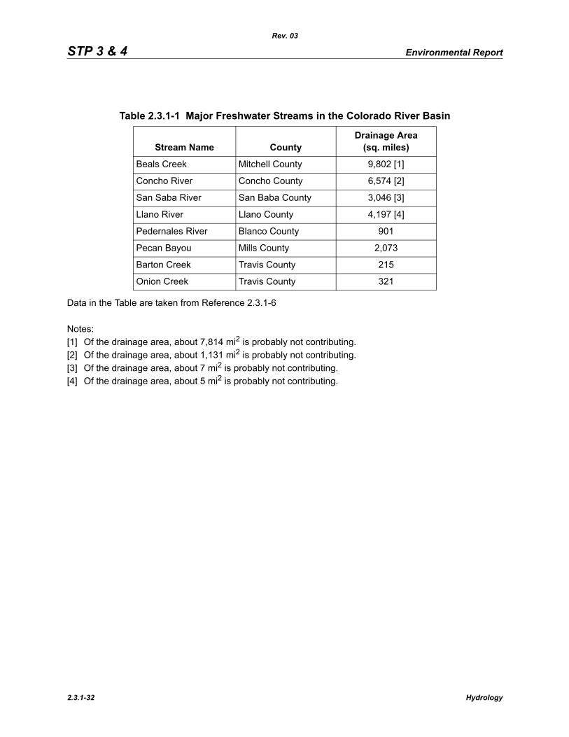
STP 3 & 4 Environmental Report
Rev. 03
Data in the Table are taken from Reference 2.3.1-6
Notes: [1] Of the drainage area, about 7,814 mi2 is probably not contributing.[2] Of the drainage area, about 1,131 mi2 is probably not contributing.[3] Of the drainage area, about 7 mi2 is probably not contributing.[4] Of the drainage area, about 5 mi2 is probably not contributing.
Table 2.3.1-1 Major Freshwater Streams in the Colorado River Basin
Stream Name CountyDrainage Area
(sq. miles)
Beals Creek Mitchell County 9,802 [1]
Concho River Concho County 6,574 [2]
San Saba River San Baba County 3,046 [3]
Llano River Llano County 4,197 [4]
Pedernales River Blanco County 901
Pecan Bayou Mills County 2,073
Barton Creek Travis County 215
Onion Creek Travis County 321
2.3.1-32 Hydrology
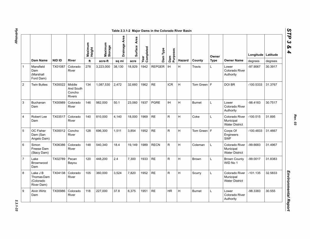
Hydrology
2.3.1-33
STP 3 & 4
Environmental R
eport
ner e Owner Name
Longitude Latitude
degrees degrees
1 Lower Colorado River Authority
-97.9067 30.3917
2 DOI BR -100.5333 31.3767
3 Lower Colorado River Authority
-98.4183 30.7517
4 Colorado River Municipal Water District
-100.515 31.895
5 Corps Of Engineers SWF
-100.4833 31.4667
6 Colorado River Municipal Water District
-99.6683 31.4967
7 Brown County WID No 1
-99.0017 31.8383
8 Colorado River Municipal Water District
-101.135 32.5833
9 Lower Colorado River Authority
-98.3383 30.555
Rev. 03
Table 2.3.1-2 Major Dams in the Colorado River Basin
Dam Name NID ID River
Max
imum
H
eigh
t
Max
imum
St
orag
e
Dra
inag
e A
rea
Surf
ace
Are
a
Year
Com
plet
ed
Dam
Typ
e
Dam
Pu
rpos
es
Hazard CountyOwTypft acre-ft sq mi acre
Mansfield Dam (Marshall Ford Dam)
TX01087 Colorado River
278 3,223,000 38,130 18,929 1942 REPGER IH H Travis L
Twin Buttes TX00022 Middle And South Concho Rivers
134 1,087,530 2,472 32,660 1962 RE ICR H Tom Green F
Buchanan Dam
TX00989 Colorado River
146 982,000 50.1 23,060 1937 PGRE IH H Burnet L
Robert Lee Dam
TX03517 Colorado River
140 810,000 4,140 18,000 1969 RE R H Coke L
OC Fisher Dam (San Angelo Dam)
TX00012 Concho River
128 696,300 1,511 3,854 1952 RE R H Tom Green F
Simon Freese Dam (Stacy Dam)
TX06386 Colorado River
148 540,340 18.4 19,149 1989 RECN R H Coleman L
Lake Brownwood Dam
TX02789 Pecan Bayou
120 448,200 2.4 7,300 1933 RE R H Brown L
Lake J B Thomas Dam (Colorado River Dam)
TX04138 Colorado River
105 360,000 3,524 7,820 1952 RE R H Scurry L
Alvin Wirtz Dam
TX00986 Colorado River
118 227,000 37.8 6,375 1951 RE HR H Burnet L
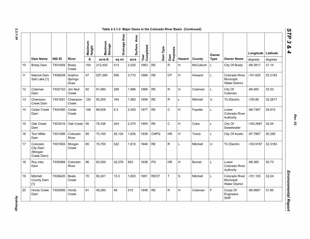
2.3.1-34H
ydrology
STP 3 & 4
Environmental R
eport
10 City Of Brady -99.3917 31.14
11 Colorado River Municipal Water District
-101.625 32.2183
12 City Of Coleman
-99.465 32.03
13 TU Electric -100.86 32.2817
14 Lower Colorado River Authority
-96.7367 29.915
15 City Of Sweetwater
-100.2667 32.04
16 City Of Austin -97.7867 30.295
17 TU Electric -100.9167 32.3183
18 Lower Colorado River Authority
-98.385 30.73
19 Colorado River Municipal Water District
-101.105 32.24
20 Corps Of Engineers SWF
-99.5667 31.85
ner e Owner Name
Longitude Latitude
degrees degrees
Rev. 03
Brady Dam TX01659 Brady Creek
104 212,400 513 2,020 1963 RE R H McCulloch L
Natural Dam Salt Lake [1]
TX06028 Sulphur Springs Draw
47 207,265 556 3,710 1989 RE CP H Howard L
Coleman Dam
TX02152 Jim Ned Creek
92 91,680 299 1,886 1966 RE R H Coleman L
Champion Creek Dam
TX01691 Champion Creek
120 90,200 164 1,560 1959 RE R L Mitchell U
Cedar Creek Dam
TX04380 Cedar Creek
106 88,628 6.3 2,400 1977 RE C H Fayette L
Oak Creek Dam
TX03516 Oak Creek 95 79,336 244 2,375 1950 RE C H Coke L
Tom Miller Dam
TX01086 Colorado River
85 73,100 26,124 1,830 1939 CNPG HR H Travis L
Colorado City Dam (Morgan Creek Dam)
TX01693 Morgan Creek
85 70,700 322 1,610 1949 RE R L Mitchell U
Roy Inks Dam
TX00988 Colorado River
96 63,500 32,076 803 1938 PG HR H Burnet L
Mitchell County Dam [1]
TX06420 Beals Creek
70 50,241 15.3 1,603 1991 REOT T S Mitchell L
Hords Creek Dam
TX00006 Hords Creek
91 49,290 48 510 1948 RE R H Coleman F
Table 2.3.1-2 Major Dams in the Colorado River Basin (Continued)
Dam Name NID ID River
Max
imum
H
eigh
t
Max
imum
St
orag
e
Dra
inag
e A
rea
Surf
ace
Are
a
Year
Com
plet
ed
Dam
Typ
e
Dam
Pu
rpos
es
Hazard CountyOwTypft acre-ft sq mi acre
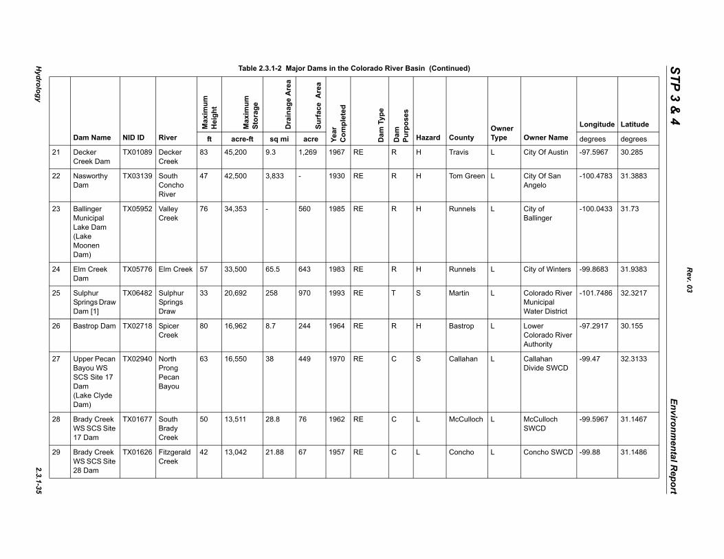
Hydrology
2.3.1-35
STP 3 & 4
Environmental R
eport
21 City Of Austin -97.5967 30.285
22 City Of San Angelo
-100.4783 31.3883
23 City of Ballinger
-100.0433 31.73
24 City of Winters -99.8683 31.9383
25 Colorado River Municipal Water District
-101.7486 32.3217
26 Lower Colorado River Authority
-97.2917 30.155
27 Callahan Divide SWCD
-99.47 32.3133
28 McCulloch SWCD
-99.5967 31.1467
29 Concho SWCD -99.88 31.1486
ner e Owner Name
Longitude Latitude
degrees degrees
Rev. 03
Decker Creek Dam
TX01089 Decker Creek
83 45,200 9.3 1,269 1967 RE R H Travis L
Nasworthy Dam
TX03139 South Concho River
47 42,500 3,833 - 1930 RE R H Tom Green L
Ballinger Municipal Lake Dam(Lake Moonen Dam)
TX05952 Valley Creek
76 34,353 - 560 1985 RE R H Runnels L
Elm Creek Dam
TX05776 Elm Creek 57 33,500 65.5 643 1983 RE R H Runnels L
Sulphur Springs Draw Dam [1]
TX06482 Sulphur Springs Draw
33 20,692 258 970 1993 RE T S Martin L
Bastrop Dam TX02718 Spicer Creek
80 16,962 8.7 244 1964 RE R H Bastrop L
Upper Pecan Bayou WS SCS Site 17 Dam (Lake Clyde Dam)
TX02940 North Prong Pecan Bayou
63 16,550 38 449 1970 RE C S Callahan L
Brady Creek WS SCS Site 17 Dam
TX01677 South Brady Creek
50 13,511 28.8 76 1962 RE C L McCulloch L
Brady Creek WS SCS Site 28 Dam
TX01626 Fitzgerald Creek
42 13,042 21.88 67 1957 RE C L Concho L
Table 2.3.1-2 Major Dams in the Colorado River Basin (Continued)
Dam Name NID ID River
Max
imum
H
eigh
t
Max
imum
St
orag
e
Dra
inag
e A
rea
Surf
ace
Are
a
Year
Com
plet
ed
Dam
Typ
e
Dam
Pu
rpos
es
Hazard CountyOwTypft acre-ft sq mi acre
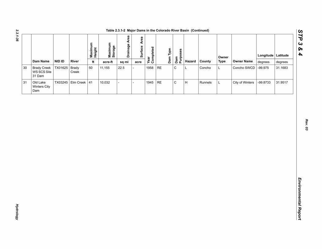
2.3.1-36H
ydrology
STP 3 & 4
Environmental R
eport
30 Concho SWCD -99.975 31.1683
31 City of Winters -99.8733 31.9517
ner e Owner Name
Longitude Latitude
degrees degrees
Rev. 03
Brady Creek WS SCS Site 31 Dam
TX01625 Brady Creek
50 11,155 22.5 - 1958 RE C L Concho L
Old Lake Winters City Dam
TX03245 Elm Creek 41 10,032 - - 1945 RE C H Runnels L
Table 2.3.1-2 Major Dams in the Colorado River Basin (Continued)
Dam Name NID ID River
Max
imum
H
eigh
t
Max
imum
St
orag
e
Dra
inag
e A
rea
Surf
ace
Are
a
Year
Com
plet
ed
Dam
Typ
e
Dam
Pu
rpos
es
Hazard CountyOwTypft acre-ft sq mi acre
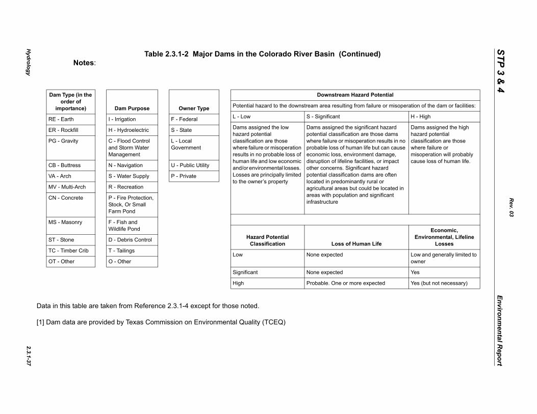
Hydrology
2.3.1-37
STP 3 & 4
Environmental R
eport
d)
Da
[1]
otential
ure or misoperation of the dam or facilities:
H - High
nt hazard ose dams
n results in no ut can cause damage, , or impact azard are often al or be located in ignificant
Dams assigned the high hazard potential classification are those where failure or misoperation will probably cause loss of human life.
ife
Economic, Environmental, Lifeline
Losses
Low and generally limited to owner
Yes
cted Yes (but not necessary)
Rev. 03
Table 2.3.1-2 Major Dams in the Colorado River Basin (ContinueNotes:
ta in this table are taken from Reference 2.3.1-4 except for those noted.
Dam data are provided by Texas Commission on Environmental Quality (TCEQ)
Dam Type (in the order of
importance) Dam Purpose Owner Type
RE - Earth I - Irrigation F - Federal
ER - Rockfill H - Hydroelectric S - State
PG - Gravity C - Flood Control and Storm Water Management
L - Local Government
CB - Buttress N - Navigation U - Public Utility
VA - Arch S - Water Supply P - Private
MV - Multi-Arch R - Recreation
CN - Concrete P - Fire Protection, Stock, Or Small Farm Pond
MS - Masonry F - Fish and Wildlife Pond
ST - Stone D - Debris Control
TC - Timber Crib T - Tailings
OT - Other O - Other
Downstream Hazard P
Potential hazard to the downstream area resulting from fail
L - Low S - Significant
Dams assigned the low hazard potential classification are those where failure or misoperation results in no probable loss of human life and low economic and/or environmental losses. Losses are principally limited to the owner’s property
Dams assigned the significapotential classification are thwhere failure or misoperatioprobable loss of human life beconomic loss, environmentdisruption of lifeline facilitiesother concerns. Significant hpotential classification damslocated in predominantly ruragricultural areas but could areas with population and sinfrastructure
Hazard Potential Classification Loss of Human L
Low None expected
Significant None expected
High Probable. One or more expe
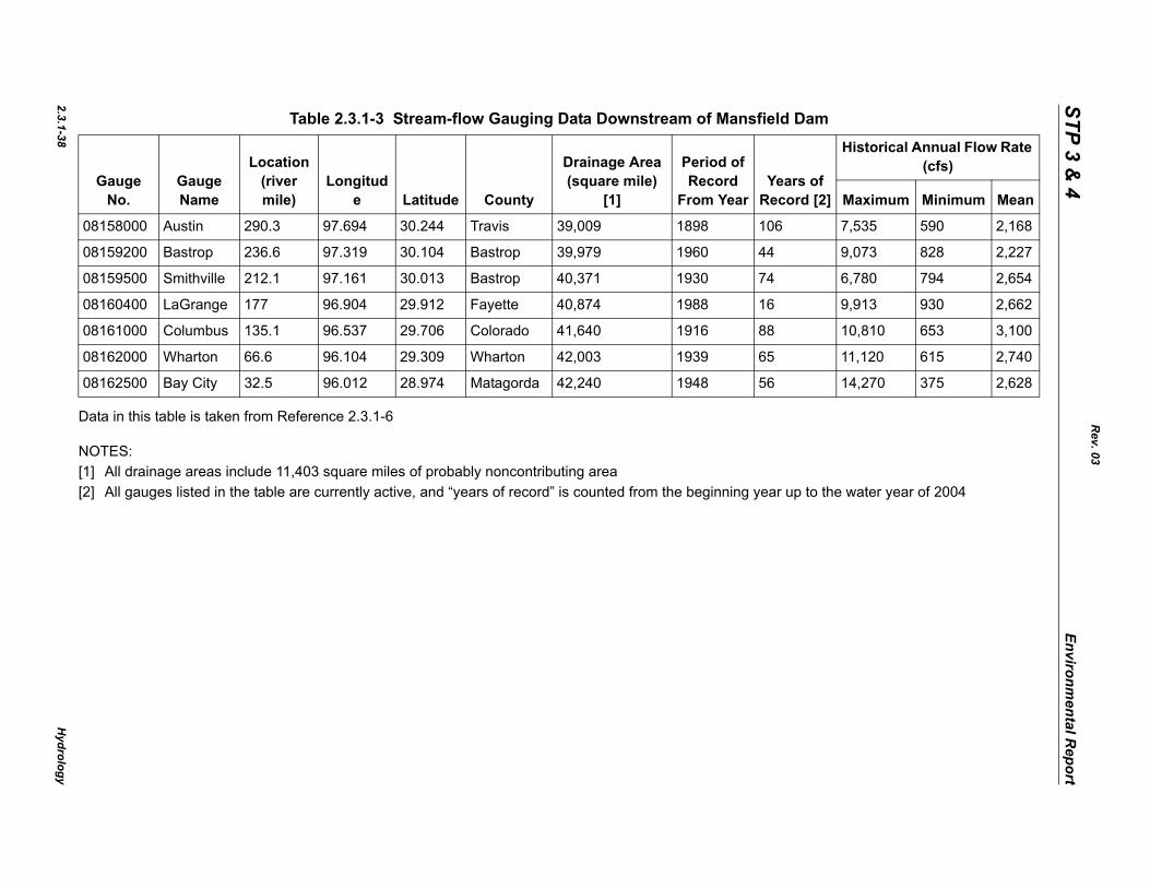
2.3.1-38H
ydrology
STP 3 & 4
Environmental R
eport
Da
NO[1][2] to the water year of 2004
am
s of d [2]
Historical Annual Flow Rate (cfs)
Maximum Minimum Mean
08 7,535 590 2,168
08 9,073 828 2,227
08 6,780 794 2,654
08 9,913 930 2,662
08 10,810 653 3,100
08 11,120 615 2,740
08 14,270 375 2,628
Rev. 03
ta in this table is taken from Reference 2.3.1-6
TES: All drainage areas include 11,403 square miles of probably noncontributing areaAll gauges listed in the table are currently active, and “years of record” is counted from the beginning year up
Table 2.3.1-3 Stream-flow Gauging Data Downstream of Mansfield D
Gauge No.
Gauge Name
Location (river mile)
Longitude Latitude County
Drainage Area (square mile)
[1]
Period of Record
From YearYear
Recor
158000 Austin 290.3 97.694 30.244 Travis 39,009 1898 106
159200 Bastrop 236.6 97.319 30.104 Bastrop 39,979 1960 44
159500 Smithville 212.1 97.161 30.013 Bastrop 40,371 1930 74
160400 LaGrange 177 96.904 29.912 Fayette 40,874 1988 16
161000 Columbus 135.1 96.537 29.706 Colorado 41,640 1916 88
162000 Wharton 66.6 96.104 29.309 Wharton 42,003 1939 65
162500 Bay City 32.5 96.012 28.974 Matagorda 42,240 1948 56
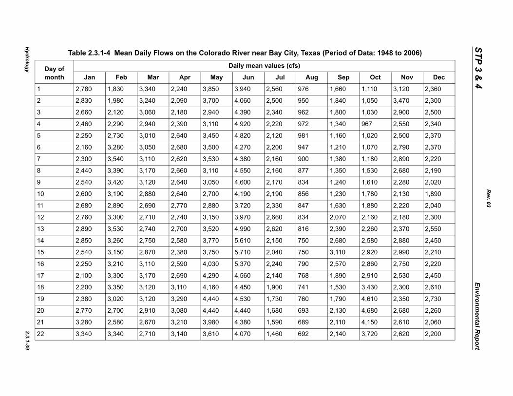
Hydrology
2.3.1-39
STP 3 & 4
Environmental R
eport
Data: 1948 to 2006)
Oct Nov Dec
1 1,110 3,120 2,360
2 1,050 3,470 2,300
3 1,030 2,900 2,500
4 967 2,550 2,340
5 1,020 2,500 2,370
6 1,070 2,790 2,370
7 1,180 2,890 2,220
8 1,530 2,680 2,190
9 1,610 2,280 2,020
10 1,780 2,130 1,890
11 1,880 2,220 2,040
12 2,160 2,180 2,300
13 2,260 2,370 2,550
14 2,580 2,880 2,450
15 2,920 2,990 2,210
16 2,860 2,750 2,220
17 2,910 2,530 2,450
18 3,430 2,300 2,610
19 4,610 2,350 2,730
20 4,680 2,680 2,260
21 4,150 2,610 2,060
22 3,720 2,620 2,200
Rev. 03
Table 2.3.1-4 Mean Daily Flows on the Colorado River near Bay City, Texas (Period of
Day ofmonth
Daily mean values (cfs)
Jan Feb Mar Apr May Jun Jul Aug Sep
2,780 1,830 3,340 2,240 3,850 3,940 2,560 976 1,660
2,830 1,980 3,240 2,090 3,700 4,060 2,500 950 1,840
2,660 2,120 3,060 2,180 2,940 4,390 2,340 962 1,800
2,460 2,290 2,940 2,390 3,110 4,920 2,220 972 1,340
2,250 2,730 3,010 2,640 3,450 4,820 2,120 981 1,160
2,160 3,280 3,050 2,680 3,500 4,270 2,200 947 1,210
2,300 3,540 3,110 2,620 3,530 4,380 2,160 900 1,380
2,440 3,390 3,170 2,660 3,110 4,550 2,160 877 1,350
2,540 3,420 3,120 2,640 3,050 4,600 2,170 834 1,240
2,600 3,190 2,880 2,640 2,700 4,190 2,190 856 1,230
2,680 2,890 2,690 2,770 2,880 3,720 2,330 847 1,630
2,760 3,300 2,710 2,740 3,150 3,970 2,660 834 2,070
2,890 3,530 2,740 2,700 3,520 4,990 2,620 816 2,390
2,850 3,260 2,750 2,580 3,770 5,610 2,150 750 2,680
2,540 3,150 2,870 2,380 3,750 5,710 2,040 750 3,110
2,250 3,210 3,110 2,590 4,030 5,370 2,240 790 2,570
2,100 3,300 3,170 2,690 4,290 4,560 2,140 768 1,890
2,200 3,350 3,120 3,110 4,160 4,450 1,900 741 1,530
2,380 3,020 3,120 3,290 4,440 4,530 1,730 760 1,790
2,770 2,700 2,910 3,080 4,440 4,440 1,680 693 2,130
3,280 2,580 2,670 3,210 3,980 4,380 1,590 689 2,110
3,340 3,340 2,710 3,140 3,610 4,070 1,460 692 2,140
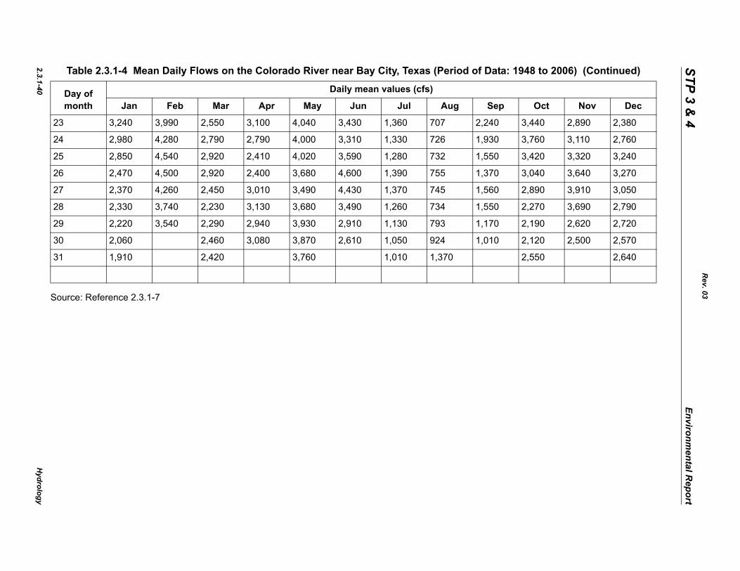
2.3.1-40H
ydrology
STP 3 & 4
Environmental R
eport
So
23 3,440 2,890 2,380
24 3,760 3,110 2,760
25 3,420 3,320 3,240
26 3,040 3,640 3,270
27 2,890 3,910 3,050
28 2,270 3,690 2,790
29 2,190 2,620 2,720
30 2,120 2,500 2,570
31 2,550 2,640
948 to 2006) (Continued)
Oct Nov Dec
Rev. 03
urce: Reference 2.3.1-7
3,240 3,990 2,550 3,100 4,040 3,430 1,360 707 2,240
2,980 4,280 2,790 2,790 4,000 3,310 1,330 726 1,930
2,850 4,540 2,920 2,410 4,020 3,590 1,280 732 1,550
2,470 4,500 2,920 2,400 3,680 4,600 1,390 755 1,370
2,370 4,260 2,450 3,010 3,490 4,430 1,370 745 1,560
2,330 3,740 2,230 3,130 3,680 3,490 1,260 734 1,550
2,220 3,540 2,290 2,940 3,930 2,910 1,130 793 1,170
2,060 2,460 3,080 3,870 2,610 1,050 924 1,010
1,910 2,420 3,760 1,010 1,370
Table 2.3.1-4 Mean Daily Flows on the Colorado River near Bay City, Texas (Period of Data: 1
Day ofmonth
Daily mean values (cfs)
Jan Feb Mar Apr May Jun Jul Aug Sep
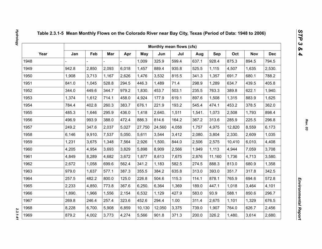
Hydrology
2.3.1-41
STP 3 & 4
Environmental R
eport
Data: 1948 to 2006)
Oct Nov Dec
19 875.3 894.5 794.5
19 4,507 1,635 2,530.
19 691.7 680.1 788.2
19 634.7 439.5 405.8
19 389.8 622.1 1,940.
19 1,315 883.9 1,625
19 453.2 378.5 362.0
19 2,508 1,793 898.4
19 285.9 225.5 296.8
19 12,820 8,559 6,173
19 2,330. 2,609 1,035
19 10,410 6,010. 4,408
19 4,944 7,059 3,708
19 1,736 4,713 3,580.
19 813.0 680.9 1,358
19 351.7 317.8 342.5
19 765.9 694.6 572.8
19 1,018 3,464 4,101
19 588.1 850.6 296.7
19 1,101 1,329 676.5
19 764.0 626.7 2,456
19 1,480. 3,614 2,680.
Rev. 03
Table 2.3.1-5 Mean Monthly Flows on the Colorado River near Bay City, Texas (Period of
Year
Monthly mean flows (cfs)
Jan Feb Mar Apr May Jun Jul Aug Sep
48 - - - - 1,009 325.9 599.4 637.1 928.4
49 942.8 2,850 2,093 6,018 1,457 889.4 935.8 525.5 1,115
50 1,908 3,713 1,167 2,626 1,476 3,532 815.5 341.3 1,357
51 841.0 1,045 528.8 294.5 446.3 1,489 71.4 298.9 1,289
52 344.0 449.6 344.7 979.2 1,830. 453.7 503.1 235.5 763.3
53 1,374 1,612 714.1 458.0 4,924 177.9 619.1 897.6 1,508
54 784.4 402.8 260.3 383.7 676.1 221.9 193.2 545.4 474.1
55 485.3 1,646 295.9 436.0 1,418 2,640. 1,511 1,541. 1,073
56 496.9 993.9 388.0 472.4 886.3 814.6 164.2 367.2 313.6
57 249.2 347.6 2,037 5,027 27,750 24,560 4,058 1,757 4,975
58 6,146 9,910. 7,537 5,050. 5,611 3,544 3,412 2,080. 3,804
59 1,231 3,675 1,348 7,564 2,926 1,500. 844.0 2,506 2,575
60 4,205 4,954 3,693 3,829 5,898 8,909 2,566 1,949 1,113
61 4,849 8,289 4,682 3,672 1,877 8,613 7,675 2,876 11,160
62 2,672 1,058 699.6 562.4 341.2 1,183 582.5 274.5 888.3
63 979.0 1,637 577.1 387.3 355.5 384.2 635.8 313.0 393.0
64 257.5 482.2 800.0 125.0 226.8 504.6 115.3 114.1 878.1
65 2,233 4,850. 773.8 367.6 6,250. 6,364 1,369 189.0 447.1
66 1,890. 1,966 1,556 2,154 6,532 1,129 427.9 583.0 93.9
67 269.8 246.4 257.4 323.6 452.6 294.4 1.00 311.4 2,675
68 8,228 6,700. 5,908 6,859 10,130 12,050 3,375 739.0 1,907
69 879.2 4,002 3,773 4,274 5,566 901.8 371.3 200.0 326.2
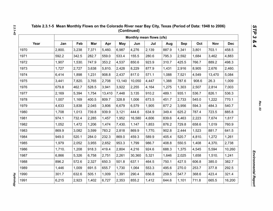
2.3.1-42H
ydrology
STP 3 & 4
Environmental R
eport
19 3,801 703.1 458.5
19 1,684 3,462 4,883
19 766.7 889.2 498.3
19 8,905 2,676 2,460.
19 4,549 13,470 5,084
19 908.6 26.3 1,009
19 2,507 2,814 7,003
19 536.7 826.1 536.3
19 545.0 1,222 770.1
19 594.3 484.3 540.7
19 787.4 723.5 885.8
19 2,223 7,674 1,617
19 658.6 1,019 760.9
19 1,523 881.7 641.5
19 4,810. 1,272 1,261
19 1,408 4,370. 2,738
19 4,545 5,594 10,260
19 1,658 1,510. 1,241
19 606.8 385.0 382.7
19 253.7 377.8 292.5
19 368.6 423.4 321.4
19 711.8 665.5 16,200
Data: 1948 to 2006)
Oct Nov Dec
Rev. 03
70 2,800. 3,238 7,371 5,460. 6,987 4,276 2,139 887.9 1,341
71 592.2 342.5 282.7 559.0 533.4 155.5 280.6 795.3 2,592
72 1,907 1,530. 747.9 353.2 4,537 850.6 923.9 310.7 425.5
73 1,727 2,727 3,638 5,810. 2,428 8,229 877.9 1,431 2,916
74 6,414 1,898 1,231 908.8 2,437 817.0 571.1 1,088 7,521
75 3,441 7,820. 3,765 2,708 13,140 10,050 4,447 1,388 787.6
76 679.8 462.7 528.5 3,941 3,922 2,255 4,164 1,275 1,303
77 2,169 5,394 1,754 13,410 7,448 3,135 910.2 489.1 935.1
78 1,007 1,169 400.5 809.7 328.8 1,006 673.5 451.7 2,733
79 4,633 3,838 2,045 3,806 6,679 6,579 1,905 877.2 3,956
80 1,708 1,013 739.8 939.9 3,121 444.6 634.9 349.4 625.2
81 974.1 732.4 2,285 1,457 1,952 16,580 4,606 839.6 4,463
82 1,052 1,472 1,206 1,474 7,430. 1,147 1,853 876.2 729.8
83 869.9 3,082 3,599 783.2 2,818 869.9 1,770. 902.8 2,444
84 949.0 520.1 284.0 232.3 869.0 459.3 589.9 405.4 520.7
85 1,979 2,052 3,955 2,652 953.3 1,799 986.7 408.8 550.5
86 1,710. 1,208 918.3 419.4 2,804 4,216 924.6 688.3 1,375
87 6,866 5,326 6,758 2,751 2,261 30,360 5,321 1,646 2,025
88 896.2 572.6 2,327 650.3 501.8 637.1 464.5 750.1 427.5
89 1,446 1,009 691.5 655.7 1,730 1,064 553.3 495.6 270.0
90 301.7 632.6 505.1 1,009 1,391 290.4 656.8 259.5 547.7
91 6,215 2,923 1,402 6,727 2,353 855.2 1,412 644.6 1,101
Table 2.3.1-5 Mean Monthly Flows on the Colorado River near Bay City, Texas (Period of (Continued)
Year
Monthly mean flows (cfs)
Jan Feb Mar Apr May Jun Jul Aug Sep
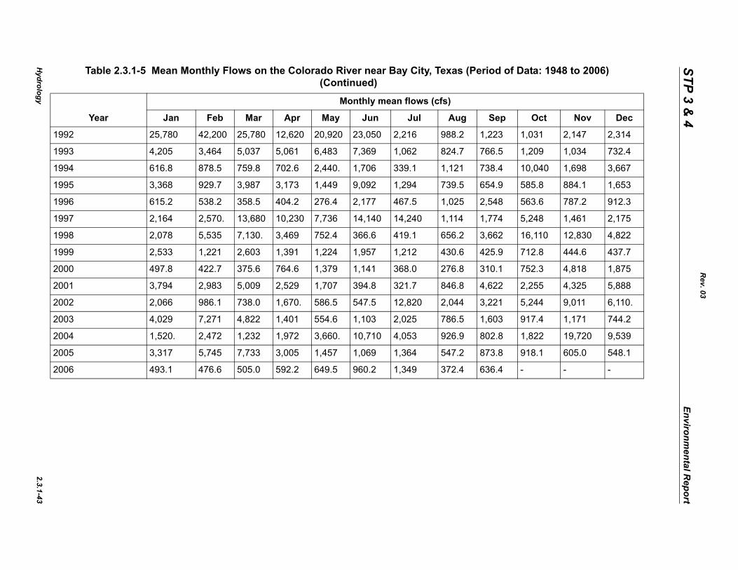
Hydrology
2.3.1-43
STP 3 & 4
Environmental R
eport
19 1,031 2,147 2,314
19 1,209 1,034 732.4
19 10,040 1,698 3,667
19 585.8 884.1 1,653
19 563.6 787.2 912.3
19 5,248 1,461 2,175
19 16,110 12,830 4,822
19 712.8 444.6 437.7
20 752.3 4,818 1,875
20 2,255 4,325 5,888
20 5,244 9,011 6,110.
20 917.4 1,171 744.2
20 1,822 19,720 9,539
20 918.1 605.0 548.1
20 - - -
Data: 1948 to 2006)
Oct Nov Dec
Rev. 03
92 25,780 42,200 25,780 12,620 20,920 23,050 2,216 988.2 1,223
93 4,205 3,464 5,037 5,061 6,483 7,369 1,062 824.7 766.5
94 616.8 878.5 759.8 702.6 2,440. 1,706 339.1 1,121 738.4
95 3,368 929.7 3,987 3,173 1,449 9,092 1,294 739.5 654.9
96 615.2 538.2 358.5 404.2 276.4 2,177 467.5 1,025 2,548
97 2,164 2,570. 13,680 10,230 7,736 14,140 14,240 1,114 1,774
98 2,078 5,535 7,130. 3,469 752.4 366.6 419.1 656.2 3,662
99 2,533 1,221 2,603 1,391 1,224 1,957 1,212 430.6 425.9
00 497.8 422.7 375.6 764.6 1,379 1,141 368.0 276.8 310.1
01 3,794 2,983 5,009 2,529 1,707 394.8 321.7 846.8 4,622
02 2,066 986.1 738.0 1,670. 586.5 547.5 12,820 2,044 3,221
03 4,029 7,271 4,822 1,401 554.6 1,103 2,025 786.5 1,603
04 1,520. 2,472 1,232 1,972 3,660. 10,710 4,053 926.9 802.8
05 3,317 5,745 7,733 3,005 1,457 1,069 1,364 547.2 873.8
06 493.1 476.6 505.0 592.2 649.5 960.2 1,349 372.4 636.4
Table 2.3.1-5 Mean Monthly Flows on the Colorado River near Bay City, Texas (Period of (Continued)
Year
Monthly mean flows (cfs)
Jan Feb Mar Apr May Jun Jul Aug Sep
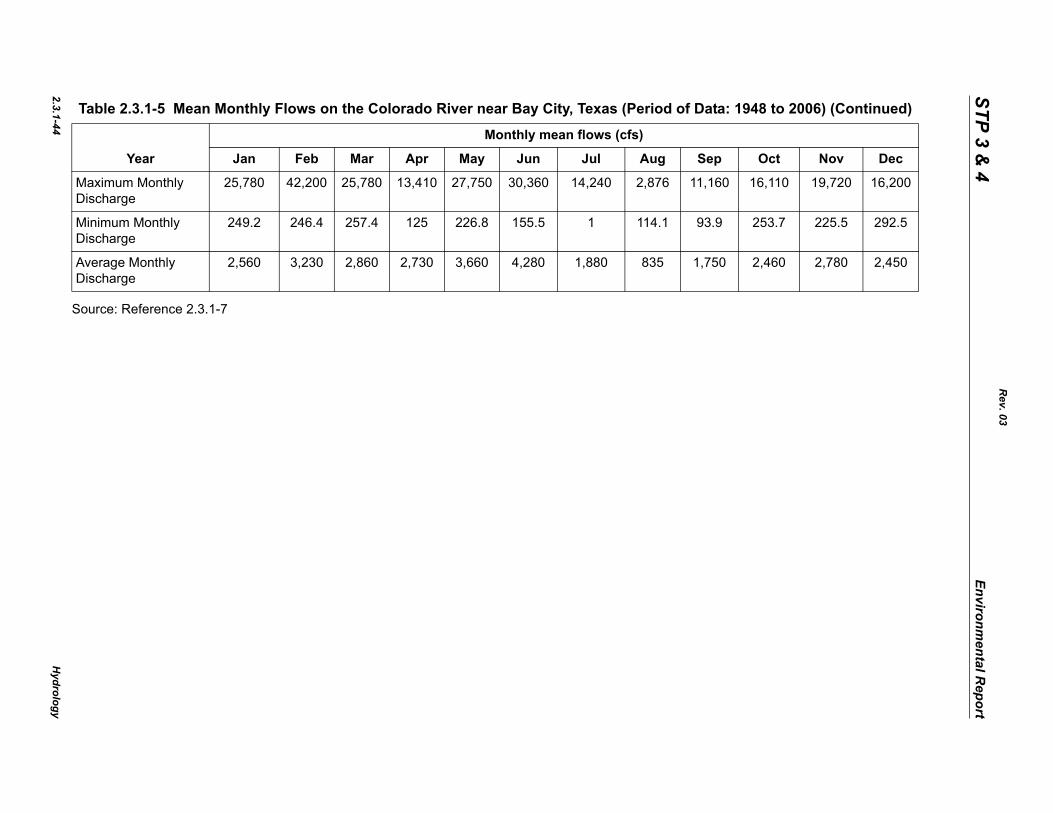
2.3.1-44H
ydrology
STP 3 & 4
Environmental R
eport
So
T 1948 to 2006) (Continued)
Oct Nov Dec
MD
16,110 19,720 16,200
MD
253.7 225.5 292.5
AD
2,460 2,780 2,450
Rev. 03
urce: Reference 2.3.1-7
able 2.3.1-5 Mean Monthly Flows on the Colorado River near Bay City, Texas (Period of Data:
Year
Monthly mean flows (cfs)
Jan Feb Mar Apr May Jun Jul Aug Sep
aximum Monthly ischarge
25,780 42,200 25,780 13,410 27,750 30,360 14,240 2,876 11,160
inimum Monthly ischarge
249.2 246.4 257.4 125 226.8 155.5 1 114.1 93.9
verage Monthly ischarge
2,560 3,230 2,860 2,730 3,660 4,280 1,880 835 1,750

Hydrology
2.3.1-45
STP 3 & 4
Environmental R
eport
of Data: 1948 to 2006)
Oct Nov Dec
19 600 655 630
19 610 1,150 1,120
19 508 498 530
19 386 400 350
19 242 290 660
19 346 431 440
19 318 342 318
19 1,080 1,020 530
19 156 128 92
19 2,130 6,180 4,400
19 1,600 1,300 710
19 2,760 3,840 3,160
19 1,170 2,350 1,700
19 1,200 1,140 2,700
19 466 449 650
19 52 253 247
19 2 3 238
19 510 1,070 1,070
19 72 282 258
19 221 304 490
19 182 428 781
19 0 2,810 1,520
Rev. 03
Table 2.3.1-6 Monthly Minimum Flows on the Colorado River near Bay City, Texas (Period
Year
Monthly minimum flows (cfs)
Jan Feb Mar Apr May Jun Jul Aug Sep
48 44 16 154 221 394
49 655 865 1,420 560 81 88 305 162 340
50 1,120 1,120 810 460 586 635 137 157 568
51 610 605 298 7 8 0 0 0 521
52 322 302 229 151 1 0 143 50 90
53 630 930 226 0 386 11 48 2 256
54 467 350 92 2 190 28 43 208 238
55 368 350 53 23 1 386 550 740 526
56 404 440 60 53 15 205 0 12 114
57 219 231 305 455 7,430 5,780 2,260 925 1,710
58 4,110 2,400 6,540 3,660 3,000 2,520 1,400 1,670 1,600
59 805 1,460 900 850 1,300 562 510 1,080 1,920
60 2,280 2,200 2,130 2,840 1,850 1,090 1,360 1,270 500
61 1,670 1,390 3,920 2,590 1,200 800 3,110 2,350 2,270
62 1,570 785 225 50 5 416 201 107 342
63 550 449 26 14 12 22 76 12 12
64 5 256 10 3 2 2 3 1 1
65 255 722 227 24 12 4,240 92 16 16
66 1,100 710 432 60 2,060 300 10 3 2
67 190 8 2 1 1 1 1 0 1
68 476 6,010 3,850 5,100 4,500 3,900 1,050 258 205
69 569 520 1,440 365 1,640 234 1 0 0
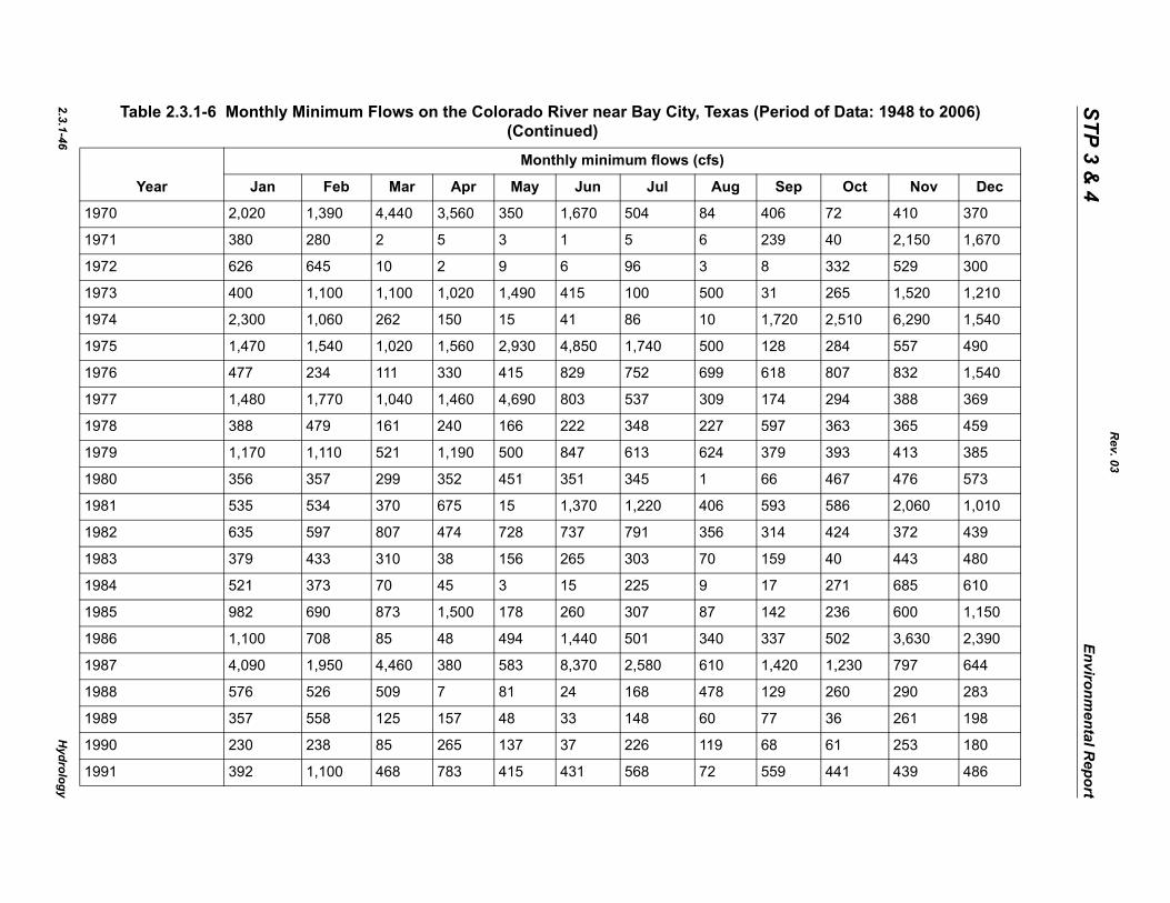
2.3.1-46H
ydrology
STP 3 & 4
Environmental R
eport
19 72 410 370
19 40 2,150 1,670
19 332 529 300
19 265 1,520 1,210
19 2,510 6,290 1,540
19 284 557 490
19 807 832 1,540
19 294 388 369
19 363 365 459
19 393 413 385
19 467 476 573
19 586 2,060 1,010
19 424 372 439
19 40 443 480
19 271 685 610
19 236 600 1,150
19 502 3,630 2,390
19 1,230 797 644
19 260 290 283
19 36 261 198
19 61 253 180
19 441 439 486
of Data: 1948 to 2006)
Oct Nov Dec
Rev. 03
70 2,020 1,390 4,440 3,560 350 1,670 504 84 406
71 380 280 2 5 3 1 5 6 239
72 626 645 10 2 9 6 96 3 8
73 400 1,100 1,100 1,020 1,490 415 100 500 31
74 2,300 1,060 262 150 15 41 86 10 1,720
75 1,470 1,540 1,020 1,560 2,930 4,850 1,740 500 128
76 477 234 111 330 415 829 752 699 618
77 1,480 1,770 1,040 1,460 4,690 803 537 309 174
78 388 479 161 240 166 222 348 227 597
79 1,170 1,110 521 1,190 500 847 613 624 379
80 356 357 299 352 451 351 345 1 66
81 535 534 370 675 15 1,370 1,220 406 593
82 635 597 807 474 728 737 791 356 314
83 379 433 310 38 156 265 303 70 159
84 521 373 70 45 3 15 225 9 17
85 982 690 873 1,500 178 260 307 87 142
86 1,100 708 85 48 494 1,440 501 340 337
87 4,090 1,950 4,460 380 583 8,370 2,580 610 1,420
88 576 526 509 7 81 24 168 478 129
89 357 558 125 157 48 33 148 60 77
90 230 238 85 265 137 37 226 119 68
91 392 1,100 468 783 415 431 568 72 559
Table 2.3.1-6 Monthly Minimum Flows on the Colorado River near Bay City, Texas (Period (Continued)
Year
Monthly minimum flows (cfs)
Jan Feb Mar Apr May Jun Jul Aug Sep
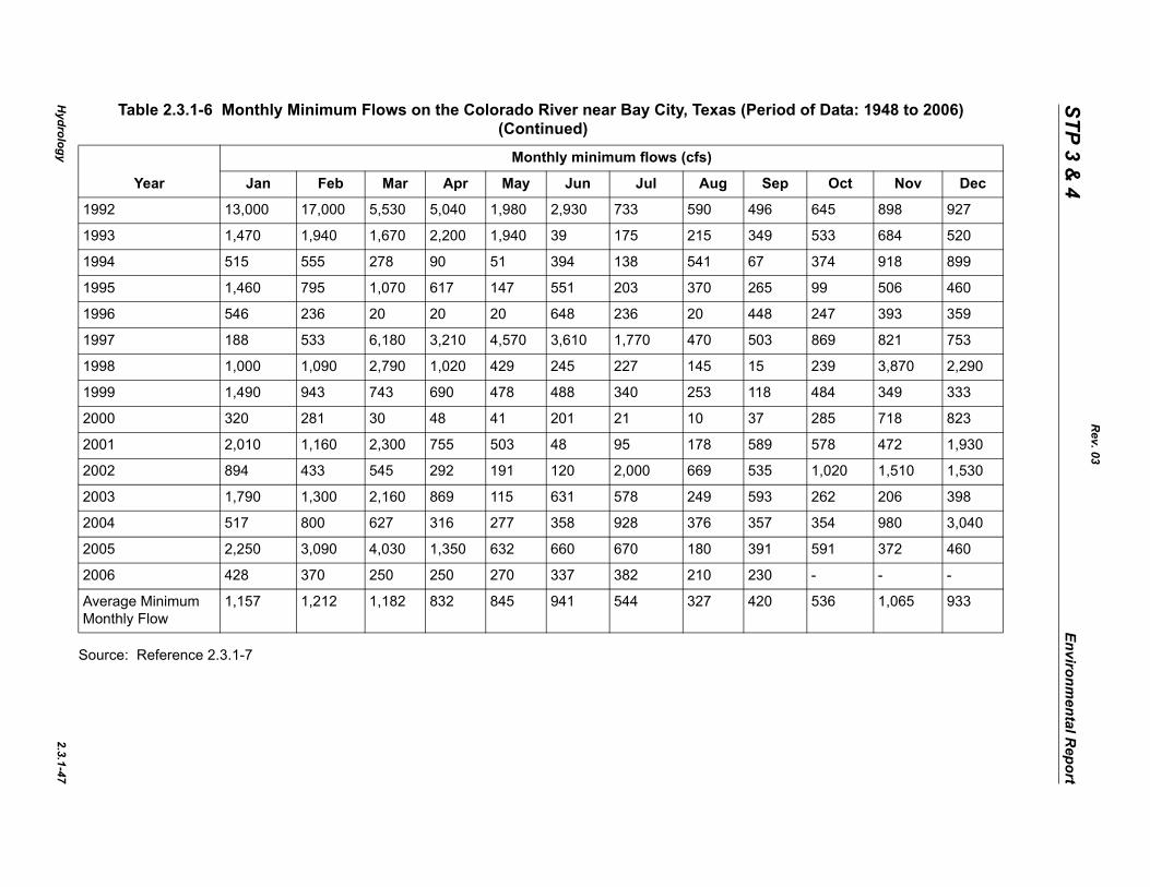
Hydrology
2.3.1-47
STP 3 & 4
Environmental R
eport
So
19 645 898 927
19 533 684 520
19 374 918 899
19 99 506 460
19 247 393 359
19 869 821 753
19 239 3,870 2,290
19 484 349 333
20 285 718 823
20 578 472 1,930
20 1,020 1,510 1,530
20 262 206 398
20 354 980 3,040
20 591 372 460
20 - - -
AM
536 1,065 933
of Data: 1948 to 2006)
Oct Nov Dec
Rev. 03
urce: Reference 2.3.1-7
92 13,000 17,000 5,530 5,040 1,980 2,930 733 590 496
93 1,470 1,940 1,670 2,200 1,940 39 175 215 349
94 515 555 278 90 51 394 138 541 67
95 1,460 795 1,070 617 147 551 203 370 265
96 546 236 20 20 20 648 236 20 448
97 188 533 6,180 3,210 4,570 3,610 1,770 470 503
98 1,000 1,090 2,790 1,020 429 245 227 145 15
99 1,490 943 743 690 478 488 340 253 118
00 320 281 30 48 41 201 21 10 37
01 2,010 1,160 2,300 755 503 48 95 178 589
02 894 433 545 292 191 120 2,000 669 535
03 1,790 1,300 2,160 869 115 631 578 249 593
04 517 800 627 316 277 358 928 376 357
05 2,250 3,090 4,030 1,350 632 660 670 180 391
06 428 370 250 250 270 337 382 210 230
verage Minimum onthly Flow
1,157 1,212 1,182 832 845 941 544 327 420
Table 2.3.1-6 Monthly Minimum Flows on the Colorado River near Bay City, Texas (Period (Continued)
Year
Monthly minimum flows (cfs)
Jan Feb Mar Apr May Jun Jul Aug Sep
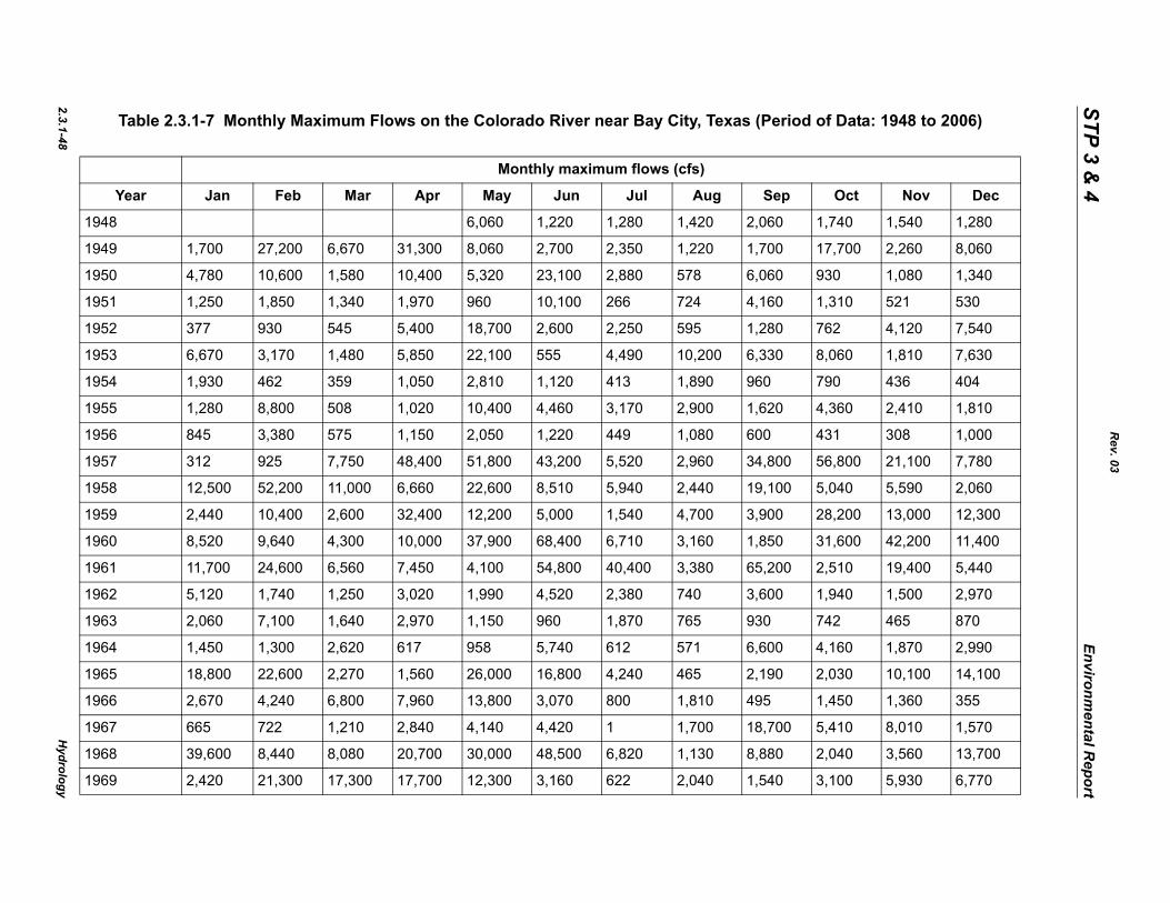
2.3.1-48H
ydrology
STP 3 & 4
Environmental R
eport
of Data: 1948 to 2006)
Oct Nov Dec
19 1,740 1,540 1,280
19 17,700 2,260 8,060
19 930 1,080 1,340
19 1,310 521 530
19 762 4,120 7,540
19 8,060 1,810 7,630
19 790 436 404
19 4,360 2,410 1,810
19 431 308 1,000
19 56,800 21,100 7,780
19 5,040 5,590 2,060
19 28,200 13,000 12,300
19 31,600 42,200 11,400
19 2,510 19,400 5,440
19 1,940 1,500 2,970
19 742 465 870
19 4,160 1,870 2,990
19 2,030 10,100 14,100
19 1,450 1,360 355
19 5,410 8,010 1,570
19 2,040 3,560 13,700
19 3,100 5,930 6,770
Rev. 03
Table 2.3.1-7 Monthly Maximum Flows on the Colorado River near Bay City, Texas (Period
Monthly maximum flows (cfs)
Year Jan Feb Mar Apr May Jun Jul Aug Sep
48 6,060 1,220 1,280 1,420 2,060
49 1,700 27,200 6,670 31,300 8,060 2,700 2,350 1,220 1,700
50 4,780 10,600 1,580 10,400 5,320 23,100 2,880 578 6,060
51 1,250 1,850 1,340 1,970 960 10,100 266 724 4,160
52 377 930 545 5,400 18,700 2,600 2,250 595 1,280
53 6,670 3,170 1,480 5,850 22,100 555 4,490 10,200 6,330
54 1,930 462 359 1,050 2,810 1,120 413 1,890 960
55 1,280 8,800 508 1,020 10,400 4,460 3,170 2,900 1,620
56 845 3,380 575 1,150 2,050 1,220 449 1,080 600
57 312 925 7,750 48,400 51,800 43,200 5,520 2,960 34,800
58 12,500 52,200 11,000 6,660 22,600 8,510 5,940 2,440 19,100
59 2,440 10,400 2,600 32,400 12,200 5,000 1,540 4,700 3,900
60 8,520 9,640 4,300 10,000 37,900 68,400 6,710 3,160 1,850
61 11,700 24,600 6,560 7,450 4,100 54,800 40,400 3,380 65,200
62 5,120 1,740 1,250 3,020 1,990 4,520 2,380 740 3,600
63 2,060 7,100 1,640 2,970 1,150 960 1,870 765 930
64 1,450 1,300 2,620 617 958 5,740 612 571 6,600
65 18,800 22,600 2,270 1,560 26,000 16,800 4,240 465 2,190
66 2,670 4,240 6,800 7,960 13,800 3,070 800 1,810 495
67 665 722 1,210 2,840 4,140 4,420 1 1,700 18,700
68 39,600 8,440 8,080 20,700 30,000 48,500 6,820 1,130 8,880
69 2,420 21,300 17,300 17,700 12,300 3,160 622 2,040 1,540
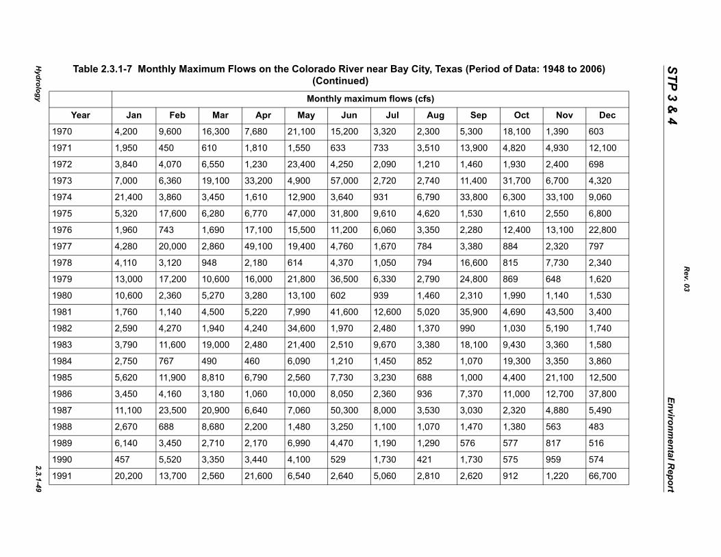
Hydrology
2.3.1-49
STP 3 & 4
Environmental R
eport
19 18,100 1,390 603
19 4,820 4,930 12,100
19 1,930 2,400 698
19 31,700 6,700 4,320
19 6,300 33,100 9,060
19 1,610 2,550 6,800
19 12,400 13,100 22,800
19 884 2,320 797
19 815 7,730 2,340
19 869 648 1,620
19 1,990 1,140 1,530
19 4,690 43,500 3,400
19 1,030 5,190 1,740
19 9,430 3,360 1,580
19 19,300 3,350 3,860
19 4,400 21,100 12,500
19 11,000 12,700 37,800
19 2,320 4,880 5,490
19 1,380 563 483
19 577 817 516
19 575 959 574
19 912 1,220 66,700
of Data: 1948 to 2006)
Oct Nov Dec
Rev. 03
70 4,200 9,600 16,300 7,680 21,100 15,200 3,320 2,300 5,300
71 1,950 450 610 1,810 1,550 633 733 3,510 13,900
72 3,840 4,070 6,550 1,230 23,400 4,250 2,090 1,210 1,460
73 7,000 6,360 19,100 33,200 4,900 57,000 2,720 2,740 11,400
74 21,400 3,860 3,450 1,610 12,900 3,640 931 6,790 33,800
75 5,320 17,600 6,280 6,770 47,000 31,800 9,610 4,620 1,530
76 1,960 743 1,690 17,100 15,500 11,200 6,060 3,350 2,280
77 4,280 20,000 2,860 49,100 19,400 4,760 1,670 784 3,380
78 4,110 3,120 948 2,180 614 4,370 1,050 794 16,600
79 13,000 17,200 10,600 16,000 21,800 36,500 6,330 2,790 24,800
80 10,600 2,360 5,270 3,280 13,100 602 939 1,460 2,310
81 1,760 1,140 4,500 5,220 7,990 41,600 12,600 5,020 35,900
82 2,590 4,270 1,940 4,240 34,600 1,970 2,480 1,370 990
83 3,790 11,600 19,000 2,480 21,400 2,510 9,670 3,380 18,100
84 2,750 767 490 460 6,090 1,210 1,450 852 1,070
85 5,620 11,900 8,810 6,790 2,560 7,730 3,230 688 1,000
86 3,450 4,160 3,180 1,060 10,000 8,050 2,360 936 7,370
87 11,100 23,500 20,900 6,640 7,060 50,300 8,000 3,530 3,030
88 2,670 688 8,680 2,200 1,480 3,250 1,100 1,070 1,470
89 6,140 3,450 2,710 2,170 6,990 4,470 1,190 1,290 576
90 457 5,520 3,350 3,440 4,100 529 1,730 421 1,730
91 20,200 13,700 2,560 21,600 6,540 2,640 5,060 2,810 2,620
Table 2.3.1-7 Monthly Maximum Flows on the Colorado River near Bay City, Texas (Period (Continued)
Monthly maximum flows (cfs)
Year Jan Feb Mar Apr May Jun Jul Aug Sep
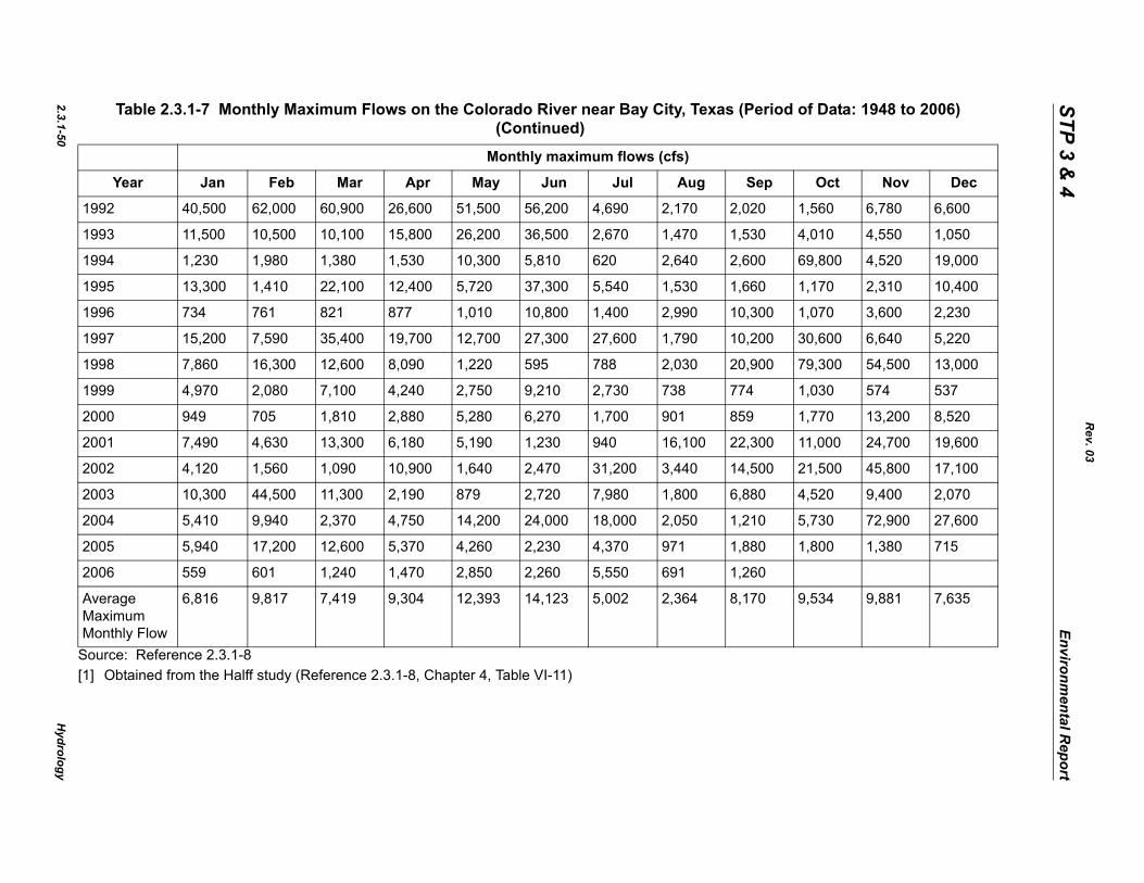
2.3.1-50H
ydrology
STP 3 & 4
Environmental R
eport
So[1]
19 1,560 6,780 6,600
19 4,010 4,550 1,050
19 69,800 4,520 19,000
19 1,170 2,310 10,400
19 1,070 3,600 2,230
19 30,600 6,640 5,220
19 79,300 54,500 13,000
19 1,030 574 537
20 1,770 13,200 8,520
20 11,000 24,700 19,600
20 21,500 45,800 17,100
20 4,520 9,400 2,070
20 5,730 72,900 27,600
20 1,800 1,380 715
20
AMM
9,534 9,881 7,635
of Data: 1948 to 2006)
Oct Nov Dec
Rev. 03
urce: Reference 2.3.1-8Obtained from the Halff study (Reference 2.3.1-8, Chapter 4, Table VI-11)
92 40,500 62,000 60,900 26,600 51,500 56,200 4,690 2,170 2,020
93 11,500 10,500 10,100 15,800 26,200 36,500 2,670 1,470 1,530
94 1,230 1,980 1,380 1,530 10,300 5,810 620 2,640 2,600
95 13,300 1,410 22,100 12,400 5,720 37,300 5,540 1,530 1,660
96 734 761 821 877 1,010 10,800 1,400 2,990 10,300
97 15,200 7,590 35,400 19,700 12,700 27,300 27,600 1,790 10,200
98 7,860 16,300 12,600 8,090 1,220 595 788 2,030 20,900
99 4,970 2,080 7,100 4,240 2,750 9,210 2,730 738 774
00 949 705 1,810 2,880 5,280 6,270 1,700 901 859
01 7,490 4,630 13,300 6,180 5,190 1,230 940 16,100 22,300
02 4,120 1,560 1,090 10,900 1,640 2,470 31,200 3,440 14,500
03 10,300 44,500 11,300 2,190 879 2,720 7,980 1,800 6,880
04 5,410 9,940 2,370 4,750 14,200 24,000 18,000 2,050 1,210
05 5,940 17,200 12,600 5,370 4,260 2,230 4,370 971 1,880
06 559 601 1,240 1,470 2,850 2,260 5,550 691 1,260
verage aximum onthly Flow
6,816 9,817 7,419 9,304 12,393 14,123 5,002 2,364 8,170
Table 2.3.1-7 Monthly Maximum Flows on the Colorado River near Bay City, Texas (Period (Continued)
Monthly maximum flows (cfs)
Year Jan Feb Mar Apr May Jun Jul Aug Sep
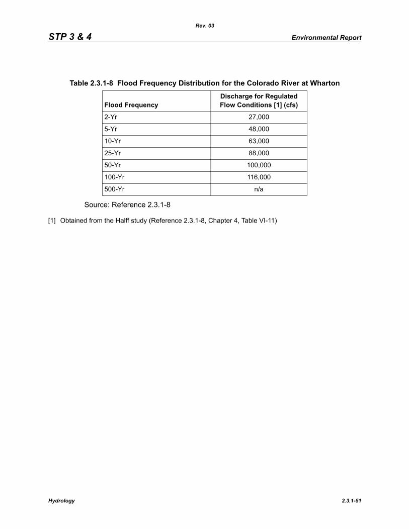
STP 3 & 4 Environmental Report
Rev. 03
Source: Reference 2.3.1-8
[1] Obtained from the Halff study (Reference 2.3.1-8, Chapter 4, Table VI-11)
Table 2.3.1-8 Flood Frequency Distribution for the Colorado River at Wharton
Flood FrequencyDischarge for Regulated Flow Conditions [1] (cfs)
2-Yr 27,000
5-Yr 48,000
10-Yr 63,000
25-Yr 88,000
50-Yr 100,000
100-Yr 116,000
500-Yr n/a
Hydrology 2.3.1-51
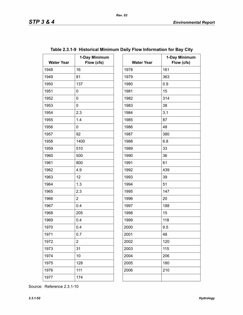
STP 3 & 4 Environmental Report
Rev. 03
Source: Reference 2.3.1-10
Table 2.3.1-9 Historical Minimum Daily Flow Information for Bay City
Water Year1-Day Minimum
Flow (cfs) Water Year1-Day Minimum
Flow (cfs)
1948 16 1978 161
1949 81 1979 363
1950 137 1980 0.9
1951 0 1981 15
1952 0 1982 314
1953 0 1983 38
1954 2.3 1984 3.1
1955 1.4 1985 87
1956 0 1986 48
1957 92 1987 380
1958 1400 1988 6.8
1959 510 1989 33
1960 500 1990 36
1961 800 1991 61
1962 4.9 1992 439
1963 12 1993 39
1964 1.3 1994 51
1965 2.3 1995 147
1966 2 1996 20
1967 0.4 1997 188
1968 205 1998 15
1969 0.4 1999 118
1970 0.4 2000 9.5
1971 0.7 2001 48
1972 2 2002 120
1973 31 2003 115
1974 10 2004 206
1975 128 2005 180
1976 111 2006 210
1977 174
2.3.1-52 Hydrology
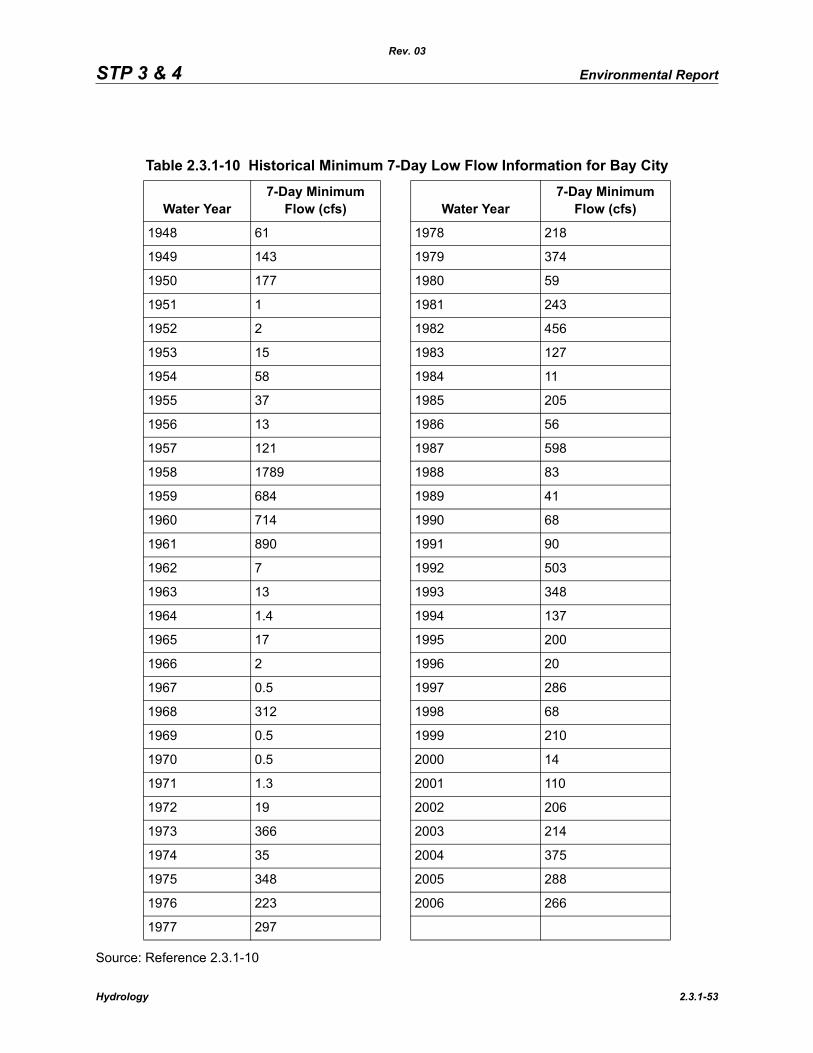
STP 3 & 4 Environmental Report
Rev. 03
Source: Reference 2.3.1-10
Table 2.3.1-10 Historical Minimum 7-Day Low Flow Information for Bay City
Water Year7-Day Minimum
Flow (cfs) Water Year7-Day Minimum
Flow (cfs)
1948 61 1978 218
1949 143 1979 374
1950 177 1980 59
1951 1 1981 243
1952 2 1982 456
1953 15 1983 127
1954 58 1984 11
1955 37 1985 205
1956 13 1986 56
1957 121 1987 598
1958 1789 1988 83
1959 684 1989 41
1960 714 1990 68
1961 890 1991 90
1962 7 1992 503
1963 13 1993 348
1964 1.4 1994 137
1965 17 1995 200
1966 2 1996 20
1967 0.5 1997 286
1968 312 1998 68
1969 0.5 1999 210
1970 0.5 2000 14
1971 1.3 2001 110
1972 19 2002 206
1973 366 2003 214
1974 35 2004 375
1975 348 2005 288
1976 223 2006 266
1977 297
Hydrology 2.3.1-53
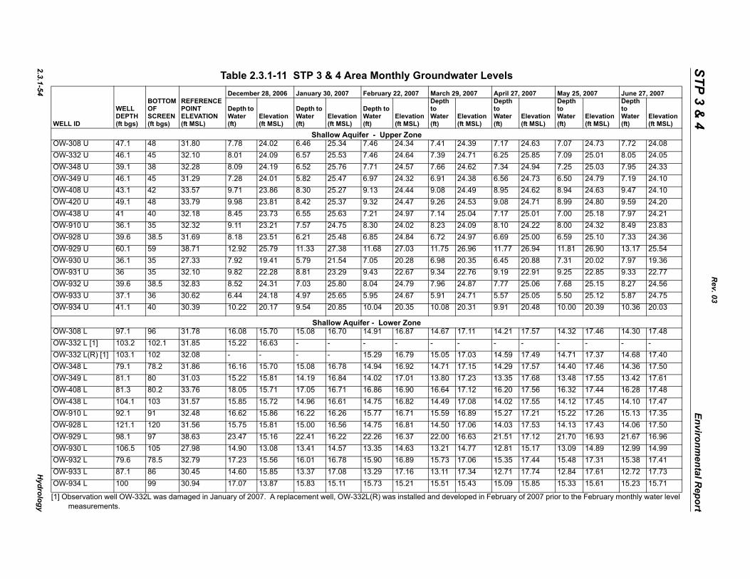
2.3.1-54H
ydrology
STP 3 & 4
Environmental R
eport
[1] f 2007 prior to the February monthly water level
WE
2007 May 25, 2007 June 27, 2007
Elevation (ft MSL)
Depth to Water (ft)
Elevation (ft MSL)
Depth to Water (ft)
Elevation (ft MSL)
OW 24.63 7.07 24.73 7.72 24.08OW 25.85 7.09 25.01 8.05 24.05OW 24.94 7.25 25.03 7.95 24.33OW 24.73 6.50 24.79 7.19 24.10OW 24.62 8.94 24.63 9.47 24.10OW 24.71 8.99 24.80 9.59 24.20OW 25.01 7.00 25.18 7.97 24.21OW 24.22 8.00 24.32 8.49 23.83OW 25.00 6.59 25.10 7.33 24.36OW 26.94 11.81 26.90 13.17 25.54OW 20.88 7.31 20.02 7.97 19.36OW 22.91 9.25 22.85 9.33 22.77OW 25.06 7.68 25.15 8.27 24.56OW 25.05 5.50 25.12 5.87 24.75OW 20.48 10.00 20.39 10.36 20.03
OW 17.57 14.32 17.46 14.30 17.48OW - - - - -OW 17.49 14.71 17.37 14.68 17.40OW 17.57 14.40 17.46 14.36 17.50OW 17.68 13.48 17.55 13.42 17.61OW 17.56 16.32 17.44 16.28 17.48OW 17.55 14.12 17.45 14.10 17.47OW 17.21 15.22 17.26 15.13 17.35OW 17.53 14.13 17.43 14.06 17.50OW 17.12 21.70 16.93 21.67 16.96OW 15.17 13.09 14.89 12.99 14.99OW 17.44 15.48 17.31 15.38 17.41OW 17.74 12.84 17.61 12.72 17.73OW 15.85 15.33 15.61 15.23 15.71
Rev. 03
Observation well OW-332L was damaged in January of 2007. A replacement well, OW-332L(R) was installed and developed in February omeasurements.
Table 2.3.1-11 STP 3 & 4 Area Monthly Groundwater Levels
LL ID
WELL DEPTH (ft bgs)
BOTTOM OF SCREEN(ft bgs)
REFERENCEPOINTELEVATION (ft MSL)
December 28, 2006 January 30, 2007 February 22, 2007 March 29, 2007 April 27,
Depth to Water (ft)
Elevation (ft MSL)
Depth to Water (ft)
Elevation (ft MSL)
Depth to Water (ft)
Elevation (ft MSL)
Depth to Water (ft)
Elevation (ft MSL)
Depth to Water (ft)
Shallow Aquifer - Upper Zone-308 U 47.1 48 31.80 7.78 24.02 6.46 25.34 7.46 24.34 7.41 24.39 7.17-332 U 46.1 45 32.10 8.01 24.09 6.57 25.53 7.46 24.64 7.39 24.71 6.25-348 U 39.1 38 32.28 8.09 24.19 6.52 25.76 7.71 24.57 7.66 24.62 7.34-349 U 46.1 45 31.29 7.28 24.01 5.82 25.47 6.97 24.32 6.91 24.38 6.56-408 U 43.1 42 33.57 9.71 23.86 8.30 25.27 9.13 24.44 9.08 24.49 8.95-420 U 49.1 48 33.79 9.98 23.81 8.42 25.37 9.32 24.47 9.26 24.53 9.08-438 U 41 40 32.18 8.45 23.73 6.55 25.63 7.21 24.97 7.14 25.04 7.17-910 U 36.1 35 32.32 9.11 23.21 7.57 24.75 8.30 24.02 8.23 24.09 8.10-928 U 39.6 38.5 31.69 8.18 23.51 6.21 25.48 6.85 24.84 6.72 24.97 6.69-929 U 60.1 59 38.71 12.92 25.79 11.33 27.38 11.68 27.03 11.75 26.96 11.77-930 U 36.1 35 27.33 7.92 19.41 5.79 21.54 7.05 20.28 6.98 20.35 6.45-931 U 36 35 32.10 9.82 22.28 8.81 23.29 9.43 22.67 9.34 22.76 9.19-932 U 39.6 38.5 32.83 8.52 24.31 7.03 25.80 8.04 24.79 7.96 24.87 7.77-933 U 37.1 36 30.62 6.44 24.18 4.97 25.65 5.95 24.67 5.91 24.71 5.57-934 U 41.1 40 30.39 10.22 20.17 9.54 20.85 10.04 20.35 10.08 20.31 9.91
Shallow Aquifer - Lower Zone-308 L 97.1 96 31.78 16.08 15.70 15.08 16.70 14.91 16.87 14.67 17.11 14.21-332 L [1] 103.2 102.1 31.85 15.22 16.63 - - - - - - --332 L(R) [1] 103.1 102 32.08 - - - - 15.29 16.79 15.05 17.03 14.59-348 L 79.1 78.2 31.86 16.16 15.70 15.08 16.78 14.94 16.92 14.71 17.15 14.29-349 L 81.1 80 31.03 15.22 15.81 14.19 16.84 14.02 17.01 13.80 17.23 13.35-408 L 81.3 80.2 33.76 18.05 15.71 17.05 16.71 16.86 16.90 16.64 17.12 16.20-438 L 104.1 103 31.57 15.85 15.72 14.96 16.61 14.75 16.82 14.49 17.08 14.02-910 L 92.1 91 32.48 16.62 15.86 16.22 16.26 15.77 16.71 15.59 16.89 15.27-928 L 121.1 120 31.56 15.75 15.81 15.00 16.56 14.75 16.81 14.50 17.06 14.03-929 L 98.1 97 38.63 23.47 15.16 22.41 16.22 22.26 16.37 22.00 16.63 21.51-930 L 106.5 105 27.98 14.90 13.08 13.41 14.57 13.35 14.63 13.21 14.77 12.81-932 L 79.6 78.5 32.79 17.23 15.56 16.01 16.78 15.90 16.89 15.73 17.06 15.35-933 L 87.1 86 30.45 14.60 15.85 13.37 17.08 13.29 17.16 13.11 17.34 12.71-934 L 100 99 30.94 17.07 13.87 15.83 15.11 15.73 15.21 15.51 15.43 15.09
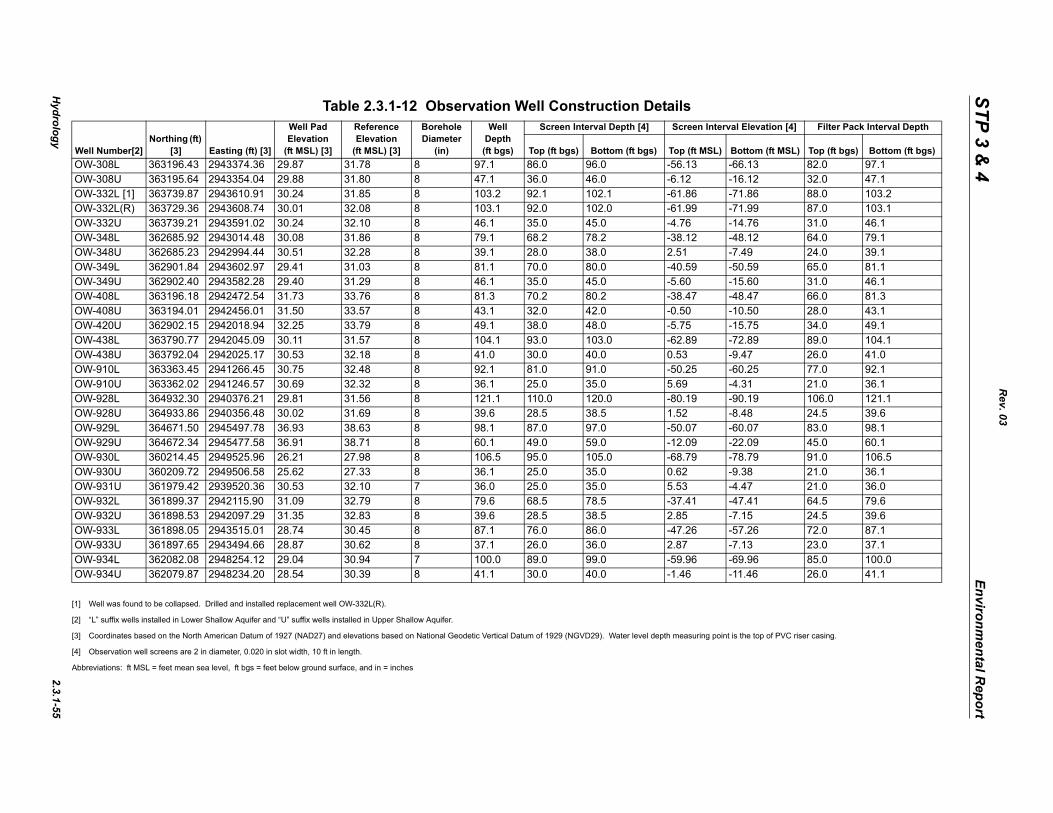
Hydrology
2.3.1-55
STP 3 & 4
Environmental R
eport
[1]
[2]
[3] is the top of PVC riser casing.
[4]
Abb
We
al Elevation [4] Filter Pack Interval Depth
Bottom (ft MSL) Top (ft bgs) Bottom (ft bgs)OW 66.13 82.0 97.1OW 16.12 32.0 47.1OW 71.86 88.0 103.2OW 71.99 87.0 103.1OW 14.76 31.0 46.1OW 48.12 64.0 79.1OW 7.49 24.0 39.1OW 50.59 65.0 81.1OW 15.60 31.0 46.1OW 48.47 66.0 81.3OW 10.50 28.0 43.1OW 15.75 34.0 49.1OW 72.89 89.0 104.1OW 9.47 26.0 41.0OW 60.25 77.0 92.1OW 4.31 21.0 36.1OW 90.19 106.0 121.1OW 8.48 24.5 39.6OW 60.07 83.0 98.1OW 22.09 45.0 60.1OW 78.79 91.0 106.5OW 9.38 21.0 36.1OW 4.47 21.0 36.0OW 47.41 64.5 79.6OW 7.15 24.5 39.6OW 57.26 72.0 87.1OW 7.13 23.0 37.1OW 69.96 85.0 100.0OW 11.46 26.0 41.1
Rev. 03
Well was found to be collapsed. Drilled and installed replacement well OW-332L(R).
“L” suffix wells installed in Lower Shallow Aquifer and “U” suffix wells installed in Upper Shallow Aquifer.
Coordinates based on the North American Datum of 1927 (NAD27) and elevations based on National Geodetic Vertical Datum of 1929 (NGVD29). Water level depth measuring point
Observation well screens are 2 in diameter, 0.020 in slot width, 10 ft in length.
reviations: ft MSL = feet mean sea level, ft bgs = feet below ground surface, and in = inches
Table 2.3.1-12 Observation Well Construction Details
ll Number[2]Northing (ft)
[3] Easting (ft) [3]
Well Pad Elevation
(ft MSL) [3]
Reference Elevation
(ft MSL) [3]
Borehole Diameter
(in)
Well Depth (ft bgs)
Screen Interval Depth [4] Screen Interv
Top (ft bgs) Bottom (ft bgs) Top (ft MSL)-308L 363196.43 2943374.36 29.87 31.78 8 97.1 86.0 96.0 -56.13 --308U 363195.64 2943354.04 29.88 31.80 8 47.1 36.0 46.0 -6.12 --332L [1] 363739.87 2943610.91 30.24 31.85 8 103.2 92.1 102.1 -61.86 --332L(R) 363729.36 2943608.74 30.01 32.08 8 103.1 92.0 102.0 -61.99 --332U 363739.21 2943591.02 30.24 32.10 8 46.1 35.0 45.0 -4.76 --348L 362685.92 2943014.48 30.08 31.86 8 79.1 68.2 78.2 -38.12 --348U 362685.23 2942994.44 30.51 32.28 8 39.1 28.0 38.0 2.51 --349L 362901.84 2943602.97 29.41 31.03 8 81.1 70.0 80.0 -40.59 --349U 362902.40 2943582.28 29.40 31.29 8 46.1 35.0 45.0 -5.60 --408L 363196.18 2942472.54 31.73 33.76 8 81.3 70.2 80.2 -38.47 --408U 363194.01 2942456.01 31.50 33.57 8 43.1 32.0 42.0 -0.50 --420U 362902.15 2942018.94 32.25 33.79 8 49.1 38.0 48.0 -5.75 --438L 363790.77 2942045.09 30.11 31.57 8 104.1 93.0 103.0 -62.89 --438U 363792.04 2942025.17 30.53 32.18 8 41.0 30.0 40.0 0.53 --910L 363363.45 2941266.45 30.75 32.48 8 92.1 81.0 91.0 -50.25 --910U 363362.02 2941246.57 30.69 32.32 8 36.1 25.0 35.0 5.69 --928L 364932.30 2940376.21 29.81 31.56 8 121.1 110.0 120.0 -80.19 --928U 364933.86 2940356.48 30.02 31.69 8 39.6 28.5 38.5 1.52 --929L 364671.50 2945497.78 36.93 38.63 8 98.1 87.0 97.0 -50.07 --929U 364672.34 2945477.58 36.91 38.71 8 60.1 49.0 59.0 -12.09 --930L 360214.45 2949525.96 26.21 27.98 8 106.5 95.0 105.0 -68.79 --930U 360209.72 2949506.58 25.62 27.33 8 36.1 25.0 35.0 0.62 --931U 361979.42 2939520.36 30.53 32.10 7 36.0 25.0 35.0 5.53 --932L 361899.37 2942115.90 31.09 32.79 8 79.6 68.5 78.5 -37.41 --932U 361898.53 2942097.29 31.35 32.83 8 39.6 28.5 38.5 2.85 --933L 361898.05 2943515.01 28.74 30.45 8 87.1 76.0 86.0 -47.26 --933U 361897.65 2943494.66 28.87 30.62 8 37.1 26.0 36.0 2.87 --934L 362082.08 2948254.12 29.04 30.94 7 100.0 89.0 99.0 -59.96 --934U 362079.87 2948234.20 28.54 30.39 8 41.1 30.0 40.0 -1.46 -
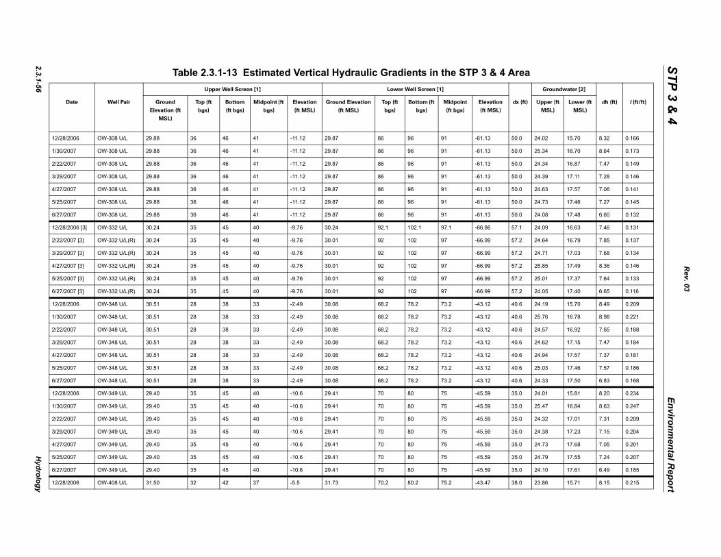
2.3.1-56H
ydrology
STP 3 & 4
Environmental R
eport
Area Groundwater [2]
dx (ft) Upper (ft
MSL)
Lower (ft
MSL)
dh (ft) i (ft/ft)
12 50.0 24.02 15.70 8.32 0.166
1/3 50.0 25.34 16.70 8.64 0.173
2/2 50.0 24.34 16.87 7.47 0.149
3/2 50.0 24.39 17.11 7.28 0.146
4/2 50.0 24.63 17.57 7.06 0.141
5/2 50.0 24.73 17.46 7.27 0.145
6/2 50.0 24.08 17.48 6.60 0.132
12 57.1 24.09 16.63 7.46 0.131
2/2 57.2 24.64 16.79 7.85 0.137
3/2 57.2 24.71 17.03 7.68 0.134
4/2 57.2 25.85 17.49 8.36 0.146
5/2 57.2 25.01 17.37 7.64 0.133
6/2 57.2 24.05 17.40 6.65 0.116
12 40.6 24.19 15.70 8.49 0.209
1/3 40.6 25.76 16.78 8.98 0.221
2/2 40.6 24.57 16.92 7.65 0.188
3/2 40.6 24.62 17.15 7.47 0.184
4/2 40.6 24.94 17.57 7.37 0.181
5/2 40.6 25.03 17.46 7.57 0.186
6/2 40.6 24.33 17.50 6.83 0.168
12 35.0 24.01 15.81 8.20 0.234
1/3 35.0 25.47 16.84 8.63 0.247
2/2 35.0 24.32 17.01 7.31 0.209
3/2 35.0 24.38 17.23 7.15 0.204
4/2 35.0 24.73 17.68 7.05 0.201
5/2 35.0 24.79 17.55 7.24 0.207
6/2 35.0 24.10 17.61 6.49 0.185
12 38.0 23.86 15.71 8.15 0.215
Rev. 03
Table 2.3.1-13 Estimated Vertical Hydraulic Gradients in the STP 3 & 4Upper Well Screen [1] Lower Well Screen [1]
Date Well Pair Ground
Elevation (ft
MSL)
Top (ft
bgs)
Bottom
(ft bgs)
Midpoint (ft
bgs)
Elevation
(ft MSL)
Ground Elevation
(ft MSL)
Top (ft
bgs)
Bottom (ft
bgs)
Midpoint
(ft bgs)
Elevation
(ft MSL)
/28/2006 OW-308 U/L 29.88 36 46 41 -11.12 29.87 86 96 91 -61.13
0/2007 OW-308 U/L 29.88 36 46 41 -11.12 29.87 86 96 91 -61.13
2/2007 OW-308 U/L 29.88 36 46 41 -11.12 29.87 86 96 91 -61.13
9/2007 OW-308 U/L 29.88 36 46 41 -11.12 29.87 86 96 91 -61.13
7/2007 OW-308 U/L 29.88 36 46 41 -11.12 29.87 86 96 91 -61.13
5/2007 OW-308 U/L 29.88 36 46 41 -11.12 29.87 86 96 91 -61.13
7/2007 OW-308 U/L 29.88 36 46 41 -11.12 29.87 86 96 91 -61.13
/28/2006 [3] OW-332 U/L 30.24 35 45 40 -9.76 30.24 92.1 102.1 97.1 -66.86
2/2007 [3] OW-332 U/L(R) 30.24 35 45 40 -9.76 30.01 92 102 97 -66.99
9/2007 [3] OW-332 U/L(R) 30.24 35 45 40 -9.76 30.01 92 102 97 -66.99
7/2007 [3] OW-332 U/L(R) 30.24 35 45 40 -9.76 30.01 92 102 97 -66.99
5/2007 [3] OW-332 U/L(R) 30.24 35 45 40 -9.76 30.01 92 102 97 -66.99
7/2007 [3] OW-332 U/L(R) 30.24 35 45 40 -9.76 30.01 92 102 97 -66.99
/28/2006 OW-348 U/L 30.51 28 38 33 -2.49 30.08 68.2 78.2 73.2 -43.12
0/2007 OW-348 U/L 30.51 28 38 33 -2.49 30.08 68.2 78.2 73.2 -43.12
2/2007 OW-348 U/L 30.51 28 38 33 -2.49 30.08 68.2 78.2 73.2 -43.12
9/2007 OW-348 U/L 30.51 28 38 33 -2.49 30.08 68.2 78.2 73.2 -43.12
7/2007 OW-348 U/L 30.51 28 38 33 -2.49 30.08 68.2 78.2 73.2 -43.12
5/2007 OW-348 U/L 30.51 28 38 33 -2.49 30.08 68.2 78.2 73.2 -43.12
7/2007 OW-348 U/L 30.51 28 38 33 -2.49 30.08 68.2 78.2 73.2 -43.12
/28/2006 OW-349 U/L 29.40 35 45 40 -10.6 29.41 70 80 75 -45.59
0/2007 OW-349 U/L 29.40 35 45 40 -10.6 29.41 70 80 75 -45.59
2/2007 OW-349 U/L 29.40 35 45 40 -10.6 29.41 70 80 75 -45.59
9/2007 OW-349 U/L 29.40 35 45 40 -10.6 29.41 70 80 75 -45.59
7/2007 OW-349 U/L 29.40 35 45 40 -10.6 29.41 70 80 75 -45.59
5/2007 OW-349 U/L 29.40 35 45 40 -10.6 29.41 70 80 75 -45.59
7/2007 OW-349 U/L 29.40 35 45 40 -10.6 29.41 70 80 75 -45.59
/28/2006 OW-408 U/L 31.50 32 42 37 -5.5 31.73 70.2 80.2 75.2 -43.47
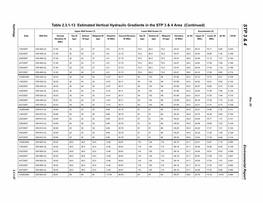
Hydrology
2.3.1-57
STP 3 & 4
Environmental R
eport
1/3 38.0 25.27 16.71 8.56 0.225
2/2 38.0 24.44 16.90 7.54 0.199
3/2 38.0 24.49 17.12 7.37 0.194
4/2 38.0 24.62 17.56 7.06 0.186
5/2 38.0 24.63 17.44 7.19 0.189
6/2 38.0 24.10 17.48 6.62 0.174
12 63.4 23.73 15.72 8.01 0.126
1/3 63.4 25.63 16.61 9.02 0.142
2/2 63.4 24.97 16.82 8.15 0.129
3/2 63.4 25.04 17.08 7.96 0.126
4/2 63.4 25.01 17.55 7.46 0.118
5/2 63.4 25.18 17.45 7.73 0.122
6/2 63.4 24.21 17.47 6.74 0.106
12 55.9 23.21 15.86 7.35 0.131
1/3 55.9 24.75 16.26 8.49 0.152
2/2 55.9 24.02 16.71 7.31 0.131
3/2 55.9 24.09 16.89 7.20 0.129
4/2 55.9 24.22 17.21 7.01 0.125
5/2 55.9 24.32 17.26 7.06 0.126
6/2 55.9 23.83 17.35 6.48 0.116
12 81.7 23.51 15.81 7.70 0.094
1/3 81.7 25.48 16.56 8.92 0.109
2/2 81.7 24.84 16.81 8.03 0.098
3/2 81.7 24.97 17.06 7.91 0.097
4/2 81.7 25.00 17.53 7.47 0.091
5/2 81.7 25.10 17.43 7.67 0.094
6/2 81.7 24.36 17.50 6.86 0.084
12 38.0 25.79 15.16 10.63 0.280
(Continued)Groundwater [2]
dx (ft) Upper (ft
MSL)
Lower (ft
MSL)
dh (ft) i (ft/ft)
Rev. 03
0/2007 OW-408 U/L 31.50 32 42 37 -5.5 31.73 70.2 80.2 75.2 -43.47
2/2007 OW-408 U/L 31.50 32 42 37 -5.5 31.73 70.2 80.2 75.2 -43.47
9/2007 OW-408 U/L 31.50 32 42 37 -5.5 31.73 70.2 80.2 75.2 -43.47
7/2007 OW-408 U/L 31.50 32 42 37 -5.5 31.73 70.2 80.2 75.2 -43.47
5/2007 OW-408 U/L 31.50 32 42 37 -5.5 31.73 70.2 80.2 75.2 -43.47
7/2007 OW-408 U/L 31.50 32 42 37 -5.5 31.73 70.2 80.2 75.2 -43.47
/28/2006 OW-438 U/L 30.53 30 40 35 -4.47 30.11 93 103 98 -67.89
0/2007 OW-438 U/L 30.53 30 40 35 -4.47 30.11 93 103 98 -67.89
2/2007 OW-438 U/L 30.53 30 40 35 -4.47 30.11 93 103 98 -67.89
9/2007 OW-438 U/L 30.53 30 40 35 -4.47 30.11 93 103 98 -67.89
7/2007 OW-438 U/L 30.53 30 40 35 -4.47 30.11 93 103 98 -67.89
5/2007 OW-438 U/L 30.53 30 40 35 -4.47 30.11 93 103 98 -67.89
7/2007 OW-438 U/L 30.53 30 40 35 -4.47 30.11 93 103 98 -67.89
/28/2006 OW-910 U/L 30.69 25 35 30 0.69 30.75 81 91 86 -55.25
0/2007 OW-910 U/L 30.69 25 35 30 0.69 30.75 81 91 86 -55.25
2/2007 OW-910 U/L 30.69 25 35 30 0.69 30.75 81 91 86 -55.25
9/2007 OW-910 U/L 30.69 25 35 30 0.69 30.75 81 91 86 -55.25
7/2007 OW-910 U/L 30.69 25 35 30 0.69 30.75 81 91 86 -55.25
5/2007 OW-910 U/L 30.69 25 35 30 0.69 30.75 81 91 86 -55.25
7/2007 OW-910 U/L 30.69 25 35 30 0.69 30.75 81 91 86 -55.25
/28/2006 OW-928 U/L 30.02 28.5 38.5 33.5 -3.48 29.81 110 120 115 -85.19
0/2007 OW-928 U/L 30.02 28.5 38.5 33.5 -3.48 29.81 110 120 115 -85.19
2/2007 OW-928 U/L 30.02 28.5 38.5 33.5 -3.48 29.81 110 120 115 -85.19
9/2007 OW-928 U/L 30.02 28.5 38.5 33.5 -3.48 29.81 110 120 115 -85.19
7/2007 OW-928 U/L 30.02 28.5 38.5 33.5 -3.48 29.81 110 120 115 -85.19
5/2007 OW-928 U/L 30.02 28.5 38.5 33.5 -3.48 29.81 110 120 115 -85.19
7/2007 OW-928 U/L 30.02 28.5 38.5 33.5 -3.48 29.81 110 120 115 -85.19
/28/2006 OW-929 U/L 36.91 49 59 54 -17.09 36.93 87 97 92 -55.07
Table 2.3.1-13 Estimated Vertical Hydraulic Gradients in the STP 3 & 4 Area Upper Well Screen [1] Lower Well Screen [1]
Date Well Pair Ground
Elevation (ft
MSL)
Top (ft
bgs)
Bottom
(ft bgs)
Midpoint (ft
bgs)
Elevation
(ft MSL)
Ground Elevation
(ft MSL)
Top (ft
bgs)
Bottom (ft
bgs)
Midpoint
(ft bgs)
Elevation
(ft MSL)
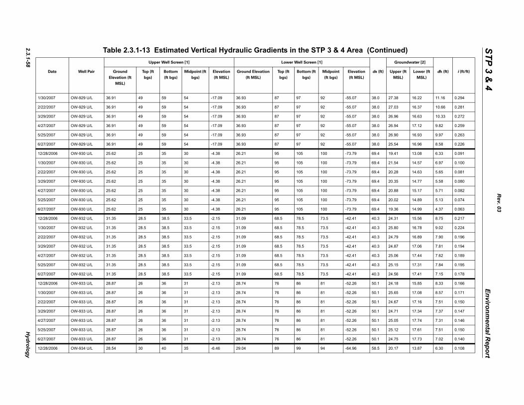
2.3.1-58H
ydrology
STP 3 & 4
Environmental R
eport
1/3 38.0 27.38 16.22 11.16 0.294
2/2 38.0 27.03 16.37 10.66 0.281
3/2 38.0 26.96 16.63 10.33 0.272
4/2 38.0 26.94 17.12 9.82 0.259
5/2 38.0 26.90 16.93 9.97 0.263
6/2 38.0 25.54 16.96 8.58 0.226
12 69.4 19.41 13.08 6.33 0.091
1/3 69.4 21.54 14.57 6.97 0.100
2/2 69.4 20.28 14.63 5.65 0.081
3/2 69.4 20.35 14.77 5.58 0.080
4/2 69.4 20.88 15.17 5.71 0.082
5/2 69.4 20.02 14.89 5.13 0.074
6/2 69.4 19.36 14.99 4.37 0.063
12 40.3 24.31 15.56 8.75 0.217
1/3 40.3 25.80 16.78 9.02 0.224
2/2 40.3 24.79 16.89 7.90 0.196
3/2 40.3 24.87 17.06 7.81 0.194
4/2 40.3 25.06 17.44 7.62 0.189
5/2 40.3 25.15 17.31 7.84 0.195
6/2 40.3 24.56 17.41 7.15 0.178
12 50.1 24.18 15.85 8.33 0.166
1/3 50.1 25.65 17.08 8.57 0.171
2/2 50.1 24.67 17.16 7.51 0.150
3/2 50.1 24.71 17.34 7.37 0.147
4/2 50.1 25.05 17.74 7.31 0.146
5/2 50.1 25.12 17.61 7.51 0.150
6/2 50.1 24.75 17.73 7.02 0.140
12 58.5 20.17 13.87 6.30 0.108
(Continued)Groundwater [2]
dx (ft) Upper (ft
MSL)
Lower (ft
MSL)
dh (ft) i (ft/ft)
Rev. 03
0/2007 OW-929 U/L 36.91 49 59 54 -17.09 36.93 87 97 92 -55.07
2/2007 OW-929 U/L 36.91 49 59 54 -17.09 36.93 87 97 92 -55.07
9/2007 OW-929 U/L 36.91 49 59 54 -17.09 36.93 87 97 92 -55.07
7/2007 OW-929 U/L 36.91 49 59 54 -17.09 36.93 87 97 92 -55.07
5/2007 OW-929 U/L 36.91 49 59 54 -17.09 36.93 87 97 92 -55.07
7/2007 OW-929 U/L 36.91 49 59 54 -17.09 36.93 87 97 92 -55.07
/28/2006 OW-930 U/L 25.62 25 35 30 -4.38 26.21 95 105 100 -73.79
0/2007 OW-930 U/L 25.62 25 35 30 -4.38 26.21 95 105 100 -73.79
2/2007 OW-930 U/L 25.62 25 35 30 -4.38 26.21 95 105 100 -73.79
9/2007 OW-930 U/L 25.62 25 35 30 -4.38 26.21 95 105 100 -73.79
7/2007 OW-930 U/L 25.62 25 35 30 -4.38 26.21 95 105 100 -73.79
5/2007 OW-930 U/L 25.62 25 35 30 -4.38 26.21 95 105 100 -73.79
7/2007 OW-930 U/L 25.62 25 35 30 -4.38 26.21 95 105 100 -73.79
/28/2006 OW-932 U/L 31.35 28.5 38.5 33.5 -2.15 31.09 68.5 78.5 73.5 -42.41
0/2007 OW-932 U/L 31.35 28.5 38.5 33.5 -2.15 31.09 68.5 78.5 73.5 -42.41
2/2007 OW-932 U/L 31.35 28.5 38.5 33.5 -2.15 31.09 68.5 78.5 73.5 -42.41
9/2007 OW-932 U/L 31.35 28.5 38.5 33.5 -2.15 31.09 68.5 78.5 73.5 -42.41
7/2007 OW-932 U/L 31.35 28.5 38.5 33.5 -2.15 31.09 68.5 78.5 73.5 -42.41
5/2007 OW-932 U/L 31.35 28.5 38.5 33.5 -2.15 31.09 68.5 78.5 73.5 -42.41
7/2007 OW-932 U/L 31.35 28.5 38.5 33.5 -2.15 31.09 68.5 78.5 73.5 -42.41
/28/2006 OW-933 U/L 28.87 26 36 31 -2.13 28.74 76 86 81 -52.26
0/2007 OW-933 U/L 28.87 26 36 31 -2.13 28.74 76 86 81 -52.26
2/2007 OW-933 U/L 28.87 26 36 31 -2.13 28.74 76 86 81 -52.26
9/2007 OW-933 U/L 28.87 26 36 31 -2.13 28.74 76 86 81 -52.26
7/2007 OW-933 U/L 28.87 26 36 31 -2.13 28.74 76 86 81 -52.26
5/2007 OW-933 U/L 28.87 26 36 31 -2.13 28.74 76 86 81 -52.26
7/2007 OW-933 U/L 28.87 26 36 31 -2.13 28.74 76 86 81 -52.26
/28/2006 OW-934 U/L 28.54 30 40 35 -6.46 29.04 89 99 94 -64.96
Table 2.3.1-13 Estimated Vertical Hydraulic Gradients in the STP 3 & 4 Area Upper Well Screen [1] Lower Well Screen [1]
Date Well Pair Ground
Elevation (ft
MSL)
Top (ft
bgs)
Bottom
(ft bgs)
Midpoint (ft
bgs)
Elevation
(ft MSL)
Ground Elevation
(ft MSL)
Top (ft
bgs)
Bottom (ft
bgs)
Midpoint
(ft bgs)
Elevation
(ft MSL)
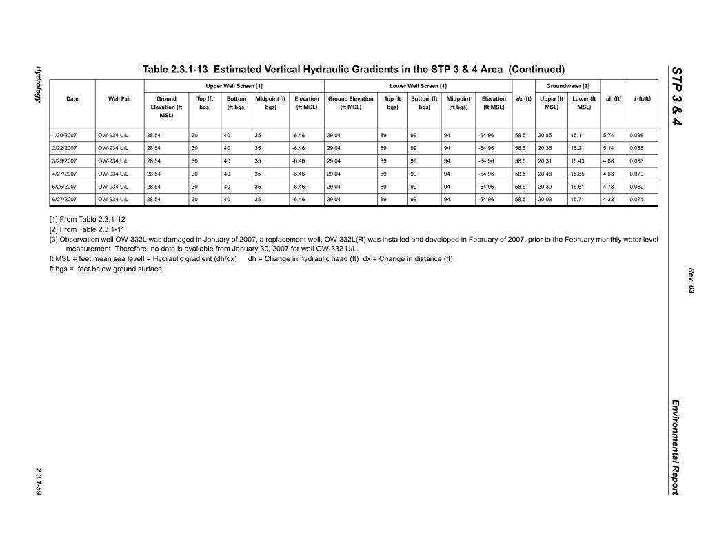
Hydrology
2.3.1-59
STP 3 & 4
Environmental R
eport
[1] [2] [3] f 2007, prior to the February monthly water level
ft Mft b
1/3 58.5 20.85 15.11 5.74 0.098
2/2 58.5 20.35 15.21 5.14 0.088
3/2 58.5 20.31 15.43 4.88 0.083
4/2 58.5 20.48 15.85 4.63 0.079
5/2 58.5 20.39 15.61 4.78 0.082
6/2 58.5 20.03 15.71 4.32 0.074
(Continued)Groundwater [2]
dx (ft) Upper (ft
MSL)
Lower (ft
MSL)
dh (ft) i (ft/ft)
Rev. 03
From Table 2.3.1-12From Table 2.3.1-11Observation well OW-332L was damaged in January of 2007, a replacement well, OW-332L(R) was installed and developed in February o
measurement. Therefore, no data is available from January 30, 2007 for well OW-332 U/L.SL = feet mean sea levelI = Hydraulic gradient (dh/dx) dh = Change in hydraulic head (ft) dx = Change in distance (ft)gs = feet below ground surface
0/2007 OW-934 U/L 28.54 30 40 35 -6.46 29.04 89 99 94 -64.96
2/2007 OW-934 U/L 28.54 30 40 35 -6.46 29.04 89 99 94 -64.96
9/2007 OW-934 U/L 28.54 30 40 35 -6.46 29.04 89 99 94 -64.96
7/2007 OW-934 U/L 28.54 30 40 35 -6.46 29.04 89 99 94 -64.96
5/2007 OW-934 U/L 28.54 30 40 35 -6.46 29.04 89 99 94 -64.96
7/2007 OW-934 U/L 28.54 30 40 35 -6.46 29.04 89 99 94 -64.96
Table 2.3.1-13 Estimated Vertical Hydraulic Gradients in the STP 3 & 4 Area Upper Well Screen [1] Lower Well Screen [1]
Date Well Pair Ground
Elevation (ft
MSL)
Top (ft
bgs)
Bottom
(ft bgs)
Midpoint (ft
bgs)
Elevation
(ft MSL)
Ground Elevation
(ft MSL)
Top (ft
bgs)
Bottom (ft
bgs)
Midpoint
(ft bgs)
Elevation
(ft MSL)
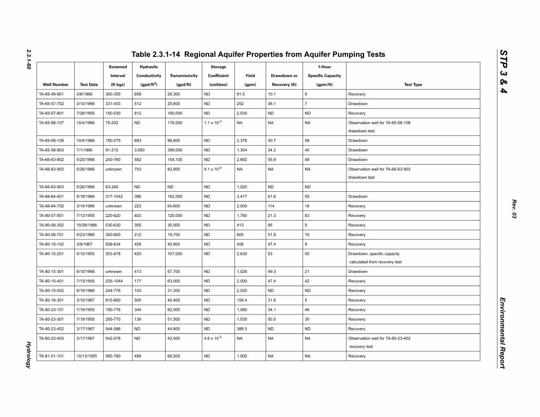
2.3.1-60H
ydrology
STP 3 & 4
Environmental R
eport
sts
W Test Type
TA
TA
TA
TA ll for TA-65-58-108
TA
TA
TA
TA ll for TA-66-63-903
TA
TA
TA
TA
TA
TA
TA
TA cific capacity
recovery test
TA
TA
TA
TA
TA
TA
TA
TA ll for TA-80-23-402
TA
Rev. 03
Table 2.3.1-14 Regional Aquifer Properties from Aquifer Pumping Te
ell Number Test Date
Screened
Interval
(ft bgs)
Hydraulic
Conductivity
(gpd/ft2)
Transmissivity
(gpd/ft)
Storage
Coefficient
(unitless)
Yield
(gpm)
Drawdown or
Recovery (ft)
1-Hour
Specific Capacity
(gpm/ft)
-65-49-901 3/8/1966 300-355 658 26,300 ND 91.5 10.1 9 Recovery
-65-57-702 3/14/1966 331-553 512 25,600 ND 252 36.1 7 Drawdown
-65-57-801 7/28/1955 150-530 812 160,000 ND 2,530 ND ND Recovery
-65-58-107 10/4/1966 75-202 ND 176,000 1.1 x 10⁻³ NA NA NA Observation we
drawdown test
-65-58-108 10/4/1966 150-275 693 86,600 ND 2,378 40.7 58 Drawdown
-65-58-803 7/1/1966 91-215 3,950 399,000 ND 1,354 34.2 40 Drawdown
-66-63-802 5/25/1966 240-760 582 154,100 ND 2,692 55.9 48 Drawdown
-66-63-902 5/26/1966 unknown 753 82,800 9.1 x 10⁻⁴ NA NA NA Observation we
drawdown test
-66-63-903 5/26/1966 63-240 ND ND ND 1,020 ND ND
-66-64-401 5/18/1966 317-1042 386 162,000 ND 3,417 61.6 55 Drawdown
-66-64-702 3/14/1966 unknown 223 64,600 ND 2,005 114 18 Recovery
-80-07-501 7/13/1955 220-820 403 120,000 ND 1,760 21.3 83 Recovery
-80-08-302 10/28/1966 530-630 355 35,500 ND 413 85 5 Recovery
-80-08-701 9/23/1966 300-600 212 19,700 ND 805 51.8 16 Recovery
-80-15-102 3/9/1967 506-634 458 45,800 ND 408 47.4 9 Recovery
-80-15-201 5/15/1955 353-878 420 107,000 ND 2,630 53 50 Drawdown, spe
calculated from
-80-15-301 6/10/1966 unknown 413 67,700 ND 1,026 49.3 21 Drawdown
-80-15-401 7/13/1955 225-1044 177 63,000 ND 2,000 47.4 42 Recovery
-80-15-502 9/19/1966 244-776 103 31,300 ND 2,020 ND ND Recovery
-80-16-301 3/10/1967 615-800 505 40,400 ND 158.4 31.6 5 Recovery
-80-23-101 7/19/1955 190-776 344 82,500 ND 1,560 34.1 46 Recovery
-80-23-301 7/19/1955 200-770 139 51,500 ND 1,535 50.5 30 Recovery
-80-23-402 3/17/1967 544-586 ND 44,800 ND 388.5 ND ND Recovery
-80-23-403 3/17/1967 542-578 ND 42,500 4.6 x 10⁻⁵ NA NA NA Observation we
recovery test
-81-01-101 10/13/1955 565-760 489 68,500 ND 1,000 NA NA Recovery
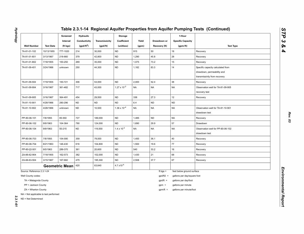
Hydrology
2.3.1-61
STP 3 & 4
Environmental R
eport
Sou
Wel
NA
ND
TA
TA
TA
TA ty calculated from
meability and
rom recovery
TA
TA ll for TA-81-09-905
TA
TA
TA ll for TA-81-10-901
PP
PP
PP ll for PP-80-06-102
PP
PP
PP
ZA
ZA
ontinued)
W Test Type
Rev. 03
rce: Reference 2.3.1-24 ft bgs = feet below ground surface
l County codes: gpd/ft2 = gallons per day/square foot
TA = Matagorda County gpd/ft = gallons per day/foot
PP = Jackson County gpm = gallons per minute
ZA = Wharton County gpm/ft = gallons per minute/foot
= Not applicable to test performed
= Not Determined
-81-01-102 10/13/1955 777-1020 214 30,000 ND 915 50 18 Recovery
-81-01-601 3/13/1967 218-660 379 42,800 ND 1,290 45.8 28 Recovery
-81-01-802 7/18/1955 150-250 269 35,000 ND 1,075 73.2 15 Recovery
-81-09-401 3/24/1966 unknown 250 44,300 ND 1,182 83.3 14 Specific capaci
drawdown, per
transmissivity f
-81-09-504 7/19/1955 150-721 306 53,000 ND 2,000 52.4 38 Recovery
-81-09-904 3/16/1967 361-482 717 43,000 1.27 x 10⁻³ NA NA NA Observation we
recovery test
-81-09-905 3/16/1967 364-491 454 29,500 ND 338 27.3 12 Recovery
-81-10-901 4/28/1966 280-296 ND ND ND 6.4 ND ND
-81-10-902 4/28/1966 unknown ND 10,500 1.36 x 10⁻⁴ NA NA NA Observation we
drawdown test
-80-06-101 7/8/1955 85-550 727 189,000 ND 1,485 ND NA Recovery
-80-06-102 9/9/1963 104-364 790 124,000 ND 1,690 29.9 57 Drawdown
-80-06-104 9/9/1963 50-215 ND 119,000 1.4 x 10⁻³ NA NA NA Observation we
drawdown test
-80-06-703 7/8/1955 154-590 359 79,000 ND 1,450 36.1 40 Recovery
-80-06-704 8/21/1963 146-430 616 104,800 ND 1,500 19.6 77 Recovery
-80-22-501 9/5/1963 288-370 361 20,600 ND 540 33.2 16 Recovery
-66-62-904 7/18/1955 162-573 382 102,000 ND 1,430 21 68 Recovery
-66-63-504 3/15/1967 167-682 475 195,300 ND 2,508 37.7 67 Recovery
Geometric Mean 420 63,640 4.7 x10⁻⁴
Table 2.3.1-14 Regional Aquifer Properties from Aquifer Pumping Tests (C
ell Number Test Date
Screened
Interval
(ft bgs)
Hydraulic
Conductivity
(gpd/ft2)
Transmissivity
(gpd/ft)
Storage
Coefficient
(unitless)
Yield
(gpm)
Drawdown or
Recovery (ft)
1-Hour
Specific Capacity
(gpm/ft)
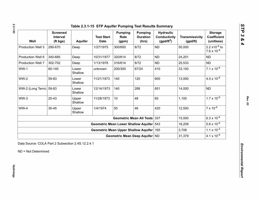
2.3.1-62H
ydrology
STP 3 & 4
Environmental R
eport
Da
ND
ransmissivity(gpd/ft)
Storage Coefficient(unitless)
P 0,000 2.2 x10⁻⁴ to7.6 x 10-4
P 4,201 ND
P 5,533 ND
W 3,150 7.1 x 10⁻⁴
W 3,000 4.5 x 10⁻⁴
W 4,000 ND
W ,100 1.7 x 10⁻³
W 2,500 7 x 10⁻⁴
5,000 6.3 x 10⁻⁴
8,209 5.6 x 10⁻⁴
,708 1.1 x 10⁻³
1,379 4.1 x 10⁻⁴
Rev. 03
ta Source: COLA Part 2 Subsection 2.4S.12.2.4.1
= Not Determined
Table 2.3.1-15 STP Aquifer Pumping Test Results Summary
Well
ScreenedInterval(ft bgs) Aquifer
Test StartDate
PumpingRate
(gpm)
Pumping Duration
(hrs)
Hydraulic Conductivity
(gpd/ft2)T
roduction Well 5 290-670 Deep 1/27/1975 300/600 8/72 ND 5
roduction Well 6 340-685 Deep 10/31/1977 320/614 8/72 ND 2
roduction Well 7 302-702 Deep 1/13/1978 316/614 8/72 ND 2
W-1 60-140 Lower Shallow
unknown 200/300 67/24 410 3
W-2 59-83 Lower Shallow
11/21/1973 140 120 600 1
W-2 (Long Term) 59-83 Lower Shallow
12/14/1973 140 288 651 1
W-3 20-43 Upper Shallow
11/28/1973 10 48 65 1
W-4 30-45 Upper Shallow
1/4/1974 50 46 420 1
Geometric Mean All Tests 337 1
Geometric Mean Lower Shallow Aquifer 543 1
Geometric Mean Upper Shallow Aquifer 165 3
Geometric Mean Deep Aquifer ND 3
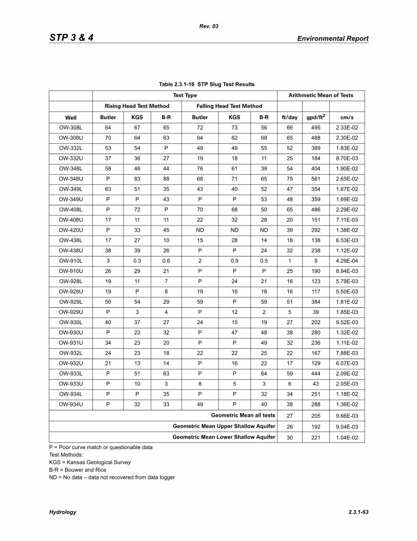
STP 3 & 4 Environmental Report
Rev. 03
P = Poor curve match or questionable dataTest Methods: KGS = Kansas Geological SurveyB-R = Bouwer and RiceND = No data – data not recovered from data logger
Table 2.3.1-16 STP Slug Test Results
Test Type Arithmetic Mean of Tests
Rising Head Test Method Falling Head Test Method
Well Butler KGS B-R Butler KGS B-R ft/day gpd/ft2 cm/s
OW-308L 64 67 65 72 73 56 66 495 2.33E-02
OW-308U 70 64 63 64 62 68 65 488 2.30E-02
OW-332L 53 54 P 49 49 55 52 389 1.83E-02
OW-332U 37 36 27 19 18 11 25 184 8.70E-03
OW-348L 58 46 44 76 61 39 54 404 1.90E-02
OW-348U P 83 88 68 71 65 75 561 2.65E-02
OW-349L 63 51 35 43 40 52 47 354 1.67E-02
OW-349U P P 43 P P 53 48 359 1.69E-02
OW-408L P 72 P 70 68 50 65 486 2.29E-02
OW-408U 17 11 11 22 32 28 20 151 7.11E-03
OW-420U P 33 45 ND ND ND 39 292 1.38E-02
OW-438L 17 27 10 15 28 14 18 138 6.53E-03
OW-438U 38 39 26 P P 24 32 238 1.12E-02
OW-910L 3 0.3 0.6 2 0.9 0.5 1 9 4.29E-04
OW-910U 26 29 21 P P P 25 190 8.94E-03
OW-928L 19 11 7 P 24 21 16 123 5.79E-03
OW-928U 19 P 8 19 16 16 16 117 5.50E-03
OW-929L 56 54 29 59 P 59 51 384 1.81E-02
OW-929U P 3 4 P 12 2 5 39 1.85E-03
OW-930L 40 37 27 24 15 19 27 202 9.52E-03
OW-930U P 23 32 P 47 48 38 280 1.32E-02
OW-931U 34 23 20 P P 49 32 236 1.11E-02
OW-932L 24 23 18 22 22 25 22 167 7.88E-03
OW-932U 21 13 14 P 16 22 17 129 6.07E-03
OW-933L P 51 63 P P 64 59 444 2.09E-02
OW-933U P 10 3 8 5 3 6 43 2.05E-03
OW-934L P P 35 P P 32 34 251 1.18E-02
OW-934U P 32 33 49 P 40 38 288 1.36E-02
Geometric Mean all tests 27 205 9.66E-03
Geometric Mean Upper Shallow Aquifer 26 192 9.04E-03
Geometric Mean Lower Shallow Aquifer 30 221 1.04E-02
Hydrology 2.3.1-63
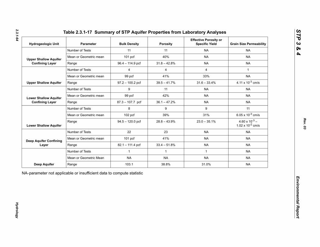
2.3.1-64H
ydrology
STP 3 & 4
Environmental R
eport
NA
s
Grain Size Permeability
NA
NA
NA
1
NA
4.11 x 10⁻³ cm/s
NA
NA
NA
11
6.05 x 10⁻³ cm/s
4.60 x 10⁻³ –1.02 x 10⁻² cm/s
NA
NA
NA
NA
NA
NA
Rev. 03
-parameter not applicable or insufficient data to compute statistic
Table 2.3.1-17 Summary of STP Aquifer Properties from Laboratory Analyse
Hydrogeologic Unit Parameter Bulk Density PorosityEffective Porosity or
Specific Yield
Upper Shallow Aquifer Confining Layer
Number of Tests 11 11 NA
Mean or Geometric mean 101 pcf 40% NA
Range 96.4 – 114.9 pcf 31.8 – 42.8% NA
Upper Shallow Aquifer
Number of Tests 4 4 4
Mean or Geometric mean 99 pcf 41% 33%
Range 97.2 – 100.2 pcf 39.5 – 41.7% 31.6 – 33.4%
Lower Shallow Aquifer Confining Layer
Number of Tests 9 11 NA
Mean or Geometric mean 99 pcf 42% NA
Range 87.3 – 107.7 pcf 36.1 – 47.2% NA
Lower Shallow Aquifer
Number of Tests 8 9 9
Mean or Geometric mean 102 pcf 39% 31%
Range 94.5 – 120.0 pcf 28.8 – 43.9% 23.0 – 35.1%
Deep Aquifer Confining Layer
Number of Tests 22 23 NA
Mean or Geometric mean 101 pcf 41% NA
Range 82.1 – 111.4 pcf 33.4 – 51.8% NA
Deep Aquifer
Number of Tests 1 1 1
Mean or Geometric Mean NA NA NA
Range 103.1 38.8% 31.0%
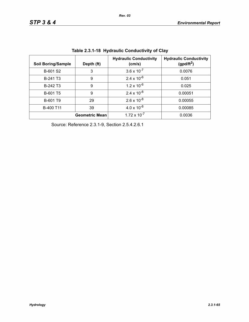
STP 3 & 4 Environmental Report
Rev. 03
Source: Reference 2.3.1-9, Section 2.5.4.2.6.1
Table 2.3.1-18 Hydraulic Conductivity of Clay
Soil Boring/Sample Depth (ft)Hydraulic Conductivity
(cm/s)Hydraulic Conductivity
(gpd/ft2)
B-601 S2 3 3.6 x 10⁻⁷ 0.0076
B-241 T3 9 2.4 x 10⁻⁶ 0.051
B-242 T3 9 1.2 x 10⁻⁶ 0.025
B-601 T5 9 2.4 x 10⁻⁸ 0.00051
B-601 T9 29 2.6 x 10⁻⁸ 0.00055
B-400 T11 39 4.0 x 10⁻⁸ 0.00085
Geometric Mean 1.72 x 10⁻⁷ 0.0036
Hydrology 2.3.1-65
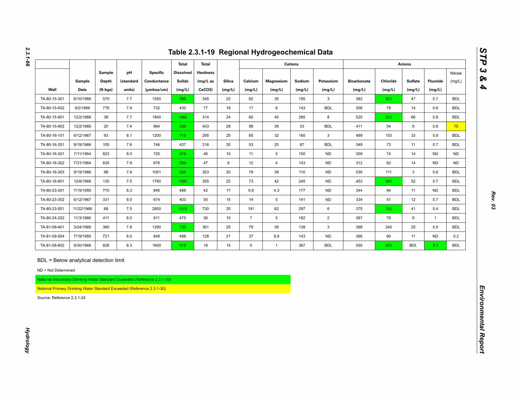
2.3.1-66H
ydrology
STP 3 & 4
Environmental R
eport
Anions
onate
/L)
Chloride
(mg/L)
Sulfate
(mg/L)
Fluoride
(mg/L)
Nitrate
(mg/L)
T 2 302 47 0.7 BDL
T 6 79 14 0.6 BDL
T 0 333 66 0.8 BDL
T 1 54 9 0.8 70
T 9 153 33 0.8 BDL
T 9 73 11 0.7 BDL
T 9 74 14 ND ND
T 2 62 14 ND ND
T 0 111 3 0.6 BDL
T 3 341 52 0.7 BDL
T 4 94 11 ND BDL
T 4 51 12 0.7 BDL
T 5 760 41 0.4 BDL
T 7 79 9 1 BDL
T 8 240 25 0.5 BDL
T 6 90 11 ND 0.2
T 0 253 BDL 3.1 BDL
BD
ND
Na
Na
So
Rev. 03
Table 2.3.1-19 Regional Hydrogeochemical Data
Sample
Date
Sample
Depth
(ft bgs)
pH
(standard
units)
Specific
Conductance
(μmhos/cm)
Total
Dissolved
Solids
(mg/L)
Total
Hardness
(mg/L as
CaCO3)
Silica
(mg/L)
Cations
Well
Calcium
(mg/L)
Magnesium
(mg/L)
Sodium
(mg/L)
Potassium
(mg/L)
Bicarb
(mg
A-80-15-301 6/10/1966 570 7.7 1550 880 348 22 82 35 195 3 38
A-80-15-502 9/2/1966 776 7.9 732 430 77 18 17 8 143 BDL 30
A-80-15-901 12/2/1966 38 7.7 1840 1060 314 24 60 40 285 8 52
A-80-15-902 12/2/1966 20 7.4 884 530 403 28 98 39 33 BDL 41
A-80-16-101 6/12/1967 93 8.1 1200 710 295 25 65 32 160 3 48
A-80-16-201 9/19/1966 100 7.6 746 437 216 20 53 20 87 BDL 34
A-80-16-301 7/11/1964 823 8.0 720 570 46 10 11 5 150 ND 30
A-80-16-302 7/31/1964 835 7.9 676 554 47 9 12 4 143 ND 31
A-80-16-303 9/19/1966 98 7.8 1051 620 353 20 79 38 110 ND 53
A-80-16-801 12/8/1966 130 7.5 1760 1000 355 22 73 42 245 ND 45
A-80-23-301 7/19/1955 770 8.3 846 488 42 17 9.9 4.3 177 ND 34
A-80-23-302 6/12/1967 331 8.0 674 403 55 15 14 5 141 ND 33
A-80-23-501 11/22/1966 68 7.5 2800 1570 730 25 191 62 297 6 37
A-80-24-202 11/3/1966 411 8.0 811 475 36 10 7 5 182 2 36
A-81-09-401 3/24/1966 360 7.8 1290 730 361 25 79 39 138 3 36
A-81-09-504 7/19/1955 721 8.0 849 498 128 21 37 8.8 143 ND 36
A-81-09-802 9/30/1966 828 8.3 1600 910 18 15 5 1 367 BDL 55
L = Below analytical detection limit
= Not Determined
tional Secondary Drinking Water Standard Exceeded (Reference 2.3.1-30)
tional Primary Drinking Water Standard Exceeded (Reference 2.3.1-30)
urce: Reference 2.3.1-24
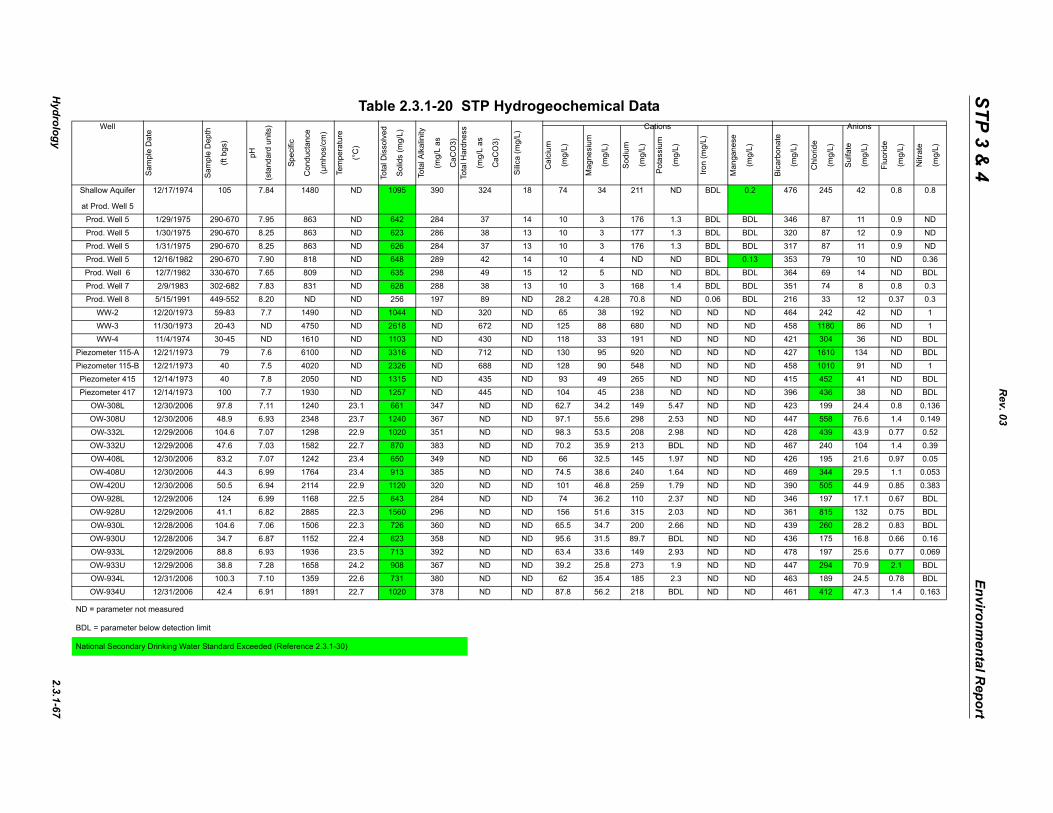
Hydrology
2.3.1-67
STP 3 & 4
Environmental R
eport
Anions
Man
gane
se
(mg/
L)
Bica
rbon
ate
(mg/
L)
Chl
orid
e
(mg/
L)
Sulfa
te
(mg/
L)
Fluo
ride
(mg/
L)
Nitr
ate
(mg/
L)
S
a
0.2 476 245 42 0.8 0.8
BDL 346 87 11 0.9 ND
BDL 320 87 12 0.9 ND
BDL 317 87 11 0.9 ND0.13 353 79 10 ND 0.36
BDL 364 69 14 ND BDL
BDL 351 74 8 0.8 0.3BDL 216 33 12 0.37 0.3
ND 464 242 42 ND 1
ND 458 1180 86 ND 1ND 421 304 36 ND BDL
Pie ND 427 1610 134 ND BDL
Pie ND 458 1010 91 ND 1P ND 415 452 41 ND BDL
P ND 396 436 38 ND BDL
ND 423 199 24.4 0.8 0.136ND 447 558 76.6 1.4 0.149
ND 428 439 43.9 0.77 0.52
ND 467 240 104 1.4 0.39ND 426 195 21.6 0.97 0.05
ND 469 344 29.5 1.1 0.053
ND 390 505 44.9 0.85 0.383ND 346 197 17.1 0.67 BDL
ND 361 815 132 0.75 BDL
ND 439 260 28.2 0.83 BDLND 436 175 16.8 0.66 0.16
ND 478 197 25.6 0.77 0.069
ND 447 294 70.9 2.1 BDLND 463 189 24.5 0.78 BDL
ND 461 412 47.3 1.4 0.163
ND
BD
Na
Rev. 03
Table 2.3.1-20 STP Hydrogeochemical DataWell
Sam
ple
Dat
e
Sam
ple
Dep
th
(ft b
gs)
pH
(sta
ndar
d un
its)
Spec
ific
Con
duct
ance
(µm
hos/
cm)
Tem
pera
ture
(°C
)
Tota
l Dis
solv
ed
Sol
ids
(mg/
L)
Tota
l Alk
alin
ity
(mg/
L as
CaC
O3)
Tota
l Har
dnes
s
(mg/
L as
CaC
O3)
Silic
a (m
g/L)
Cations
Cal
cium
(mg/
L)
Mag
nesi
um
(mg/
L)
Sod
ium
(mg/
L)
Pota
ssiu
m
(mg/
L)
Iron
(mg/
L)
hallow Aquifer
t Prod. Well 5
12/17/1974 105 7.84 1480 ND 1095 390 324 18 74 34 211 ND BDL
Prod. Well 5 1/29/1975 290-670 7.95 863 ND 642 284 37 14 10 3 176 1.3 BDL
Prod. Well 5 1/30/1975 290-670 8.25 863 ND 623 286 38 13 10 3 177 1.3 BDL
Prod. Well 5 1/31/1975 290-670 8.25 863 ND 626 284 37 13 10 3 176 1.3 BDLProd. Well 5 12/16/1982 290-670 7.90 818 ND 648 289 42 14 10 4 ND ND BDL
Prod. Well 6 12/7/1982 330-670 7.65 809 ND 635 298 49 15 12 5 ND ND BDL
Prod. Well 7 2/9/1983 302-682 7.83 831 ND 628 288 38 13 10 3 168 1.4 BDLProd. Well 8 5/15/1991 449-552 8.20 ND ND 256 197 89 ND 28.2 4.28 70.8 ND 0.06
WW-2 12/20/1973 59-83 7.7 1490 ND 1044 ND 320 ND 65 38 192 ND ND
WW-3 11/30/1973 20-43 ND 4750 ND 2618 ND 672 ND 125 88 680 ND NDWW-4 11/4/1974 30-45 ND 1610 ND 1103 ND 430 ND 118 33 191 ND ND
zometer 115-A 12/21/1973 79 7.6 6100 ND 3316 ND 712 ND 130 95 920 ND ND
zometer 115-B 12/21/1973 40 7.5 4020 ND 2326 ND 688 ND 128 90 548 ND NDiezometer 415 12/14/1973 40 7.8 2050 ND 1315 ND 435 ND 93 49 265 ND ND
iezometer 417 12/14/1973 100 7.7 1930 ND 1257 ND 445 ND 104 45 238 ND ND
OW-308L 12/30/2006 97.8 7.11 1240 23.1 661 347 ND ND 62.7 34.2 149 5.47 NDOW-308U 12/30/2006 48.9 6.93 2348 23.7 1240 367 ND ND 97.1 55.6 298 2.53 ND
OW-332L 12/29/2006 104.6 7.07 1298 22.9 1020 351 ND ND 98.3 53.5 208 2.98 ND
OW-332U 12/29/2006 47.6 7.03 1582 22.7 870 383 ND ND 70.2 35.9 213 BDL NDOW-408L 12/30/2006 83.2 7.07 1242 23.4 650 349 ND ND 66 32.5 145 1.97 ND
OW-408U 12/30/2006 44.3 6.99 1764 23.4 913 385 ND ND 74.5 38.6 240 1.64 ND
OW-420U 12/30/2006 50.5 6.94 2114 22.9 1120 320 ND ND 101 46.8 259 1.79 NDOW-928L 12/29/2006 124 6.99 1168 22.5 643 284 ND ND 74 36.2 110 2.37 ND
OW-928U 12/29/2006 41.1 6.82 2885 22.3 1560 296 ND ND 156 51.6 315 2.03 ND
OW-930L 12/28/2006 104.6 7.06 1506 22.3 726 360 ND ND 65.5 34.7 200 2.66 NDOW-930U 12/28/2006 34.7 6.87 1152 22.4 623 358 ND ND 95.6 31.5 89.7 BDL ND
OW-933L 12/29/2006 88.8 6.93 1936 23.5 713 392 ND ND 63.4 33.6 149 2.93 ND
OW-933U 12/29/2006 38.8 7.28 1658 24.2 908 367 ND ND 39.2 25.8 273 1.9 NDOW-934L 12/31/2006 100.3 7.10 1359 22.6 731 380 ND ND 62 35.4 185 2.3 ND
OW-934U 12/31/2006 42.4 6.91 1891 22.7 1020 378 ND ND 87.8 56.2 218 BDL ND
= parameter not measured
L = parameter below detection limit
tional Secondary Drinking Water Standard Exceeded (Reference 2.3.1-30)
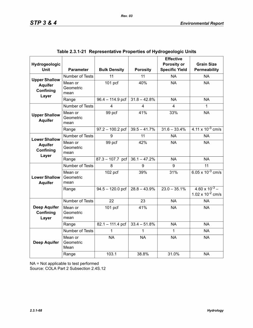
STP 3 & 4 Environmental Report
Rev. 03
NA = Not applicable to test performedSource: COLA Part 2 Subsection 2.4S.12
Table 2.3.1-21 Representative Properties of Hydrogeologic Units
Hydrogeologic Unit Parameter Bulk Density Porosity
Effective Porosity or
Specific YieldGrain Size
Permeability
Upper Shallow Aquifer
Confining Layer
Number of Tests 11 11 NA NAMean or Geometric mean
101 pcf 40% NA NA
Range 96.4 – 114.9 pcf 31.8 – 42.8% NA NA
Upper Shallow Aquifer
Number of Tests 4 4 4 1Mean or Geometric mean
99 pcf 41% 33% NA
Range 97.2 – 100.2 pcf 39.5 – 41.7% 31.6 – 33.4% 4.11 x 10⁻³ cm/s
Lower Shallow Aquifer
Confining Layer
Number of Tests 9 11 NA NAMean or Geometric mean
99 pcf 42% NA NA
Range 87.3 – 107.7 pcf 36.1 – 47.2% NA NA
Lower Shallow Aquifer
Number of Tests 8 9 9 11Mean or Geometric mean
102 pcf 39% 31% 6.05 x 10⁻³ cm/s
Range 94.5 – 120.0 pcf 28.8 – 43.9% 23.0 – 35.1% 4.60 x 10⁻³ –1.02 x 10⁻² cm/s
Deep Aquifer Confining
Layer
Number of Tests 22 23 NA NAMean or Geometric mean
101 pcf 41% NA NA
Range 82.1 – 111.4 pcf 33.4 – 51.8% NA NA
Deep Aquifer
Number of Tests 1 1 1 NAMean or Geometric Mean
NA NA NA NA
Range 103.1 38.8% 31.0% NA
2.3.1-68 Hydrology
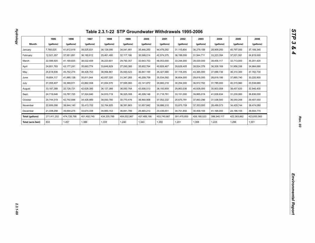
Hydrology
2.3.1-69
STP 3 & 4
Environmental R
eport
04
lons)
2005
(gallons)
2006
(gallons)
Ja 250 40,797,000 37,189,345
Fe 394 37,531,591 34,819,000
Ma 117 32,713,000 35,201,420
Ap 169 31,956,336 34,964,690
Ma 736 36,310,300 37,782,730
Ju 186 37,885,740 33,220,900
Ju 000 40,315,960 33,538,680
Au 058 38,457,620 32,946,400
Se 634 31,230,060 36,836,000
Oc 000 36,540,206 29,407,550
No 573 34,429,744 38,474,080
De 000 24,196,105 39,554,770
To ,117 422,363,662 423,935,565
To 1,296 1,301
Rev. 03
Table 2.3.1-22 STP Groundwater Withdrawals 1995-2006
Month
1995
(gallons)
1996
(gallons)
1997
(gallons)
1998
(gallons)
1999
(gallons)
2000
(gallons)
2001
(gallons)
2002
(gallons)
2003
(gallons)
20
(gal
nuary 7,765,025 41,812,919 39,525,831 36,128,090 34,041,991 35,446,250 44,476,292 31,115,804 36,279,188 28,909,
bruary 12,521,357 37,551,891 36,180,612 29,461,480 32,117,186 30,568,014 42,574,575 36,198,000 31,944,711 33,323,
rch 22,598,920 41,169,835 38,532,459 36,223,601 29,792,357 32,643,753 48,053,000 33,244,000 28,020,000 38,458,
ril 24,601,783 43,177,241 35,683,774 33,649,929 27,093,385 35,652,764 40,828,467 29,628,405 28,524,378 36,309,
y 25,618,936 45,752,274 38,428,753 38,956,861 35,593,523 36,847,100 35,327,680 37,118,205 43,365,000 27,088,
ne 19,654,117 41,995,128 35,811,044 42,057,320 31,347,265 40,259,759 35,534,592 36,604,000 29,816,000 28,819,
ly 31,055,407 35,369,911 43,862,008 41,054,570 37,595,060 43,141,872 35,660,218 30,254,000 36,912,782 31,785,
gust 33,187,388 32,728,731 42,628,395 36,127,366 36,092,764 43,008,513 38,193,859 29,863,036 45,828,000 30,803,
pt. 24,719,646 33,787,725 37,324,840 34,910,719 36,325,308 40,309,148 31,716,791 33,151,000 39,865,019 41,838,
tober 25,744,319 42,742,696 34,426,989 38,050,780 30,770,476 38,460,958 37,052,232 25,675,791 37,863,296 31,538,
vember 22,606,096 38,944,140 35,413,702 32,764,920 36,391,863 31,657,842 30,886,310 33,875,759 37,353,000 28,499,
cember 21,338,258 39,694,275 33,674,338 34,950,153 36,841,789 29,493,213 33,436,651 34,751,855 30,409,159 41,168,
tal (gallons) 271,411,252 474,726,766 451,492,745 434,335,789 404,002,967 437,489,186 453,740,667 391,479,855 426,180,533 398,540
tal (acre-feet) 833 1,457 1,386 1,333 1,240 1,343 1,392 1,201 1,308 1,223
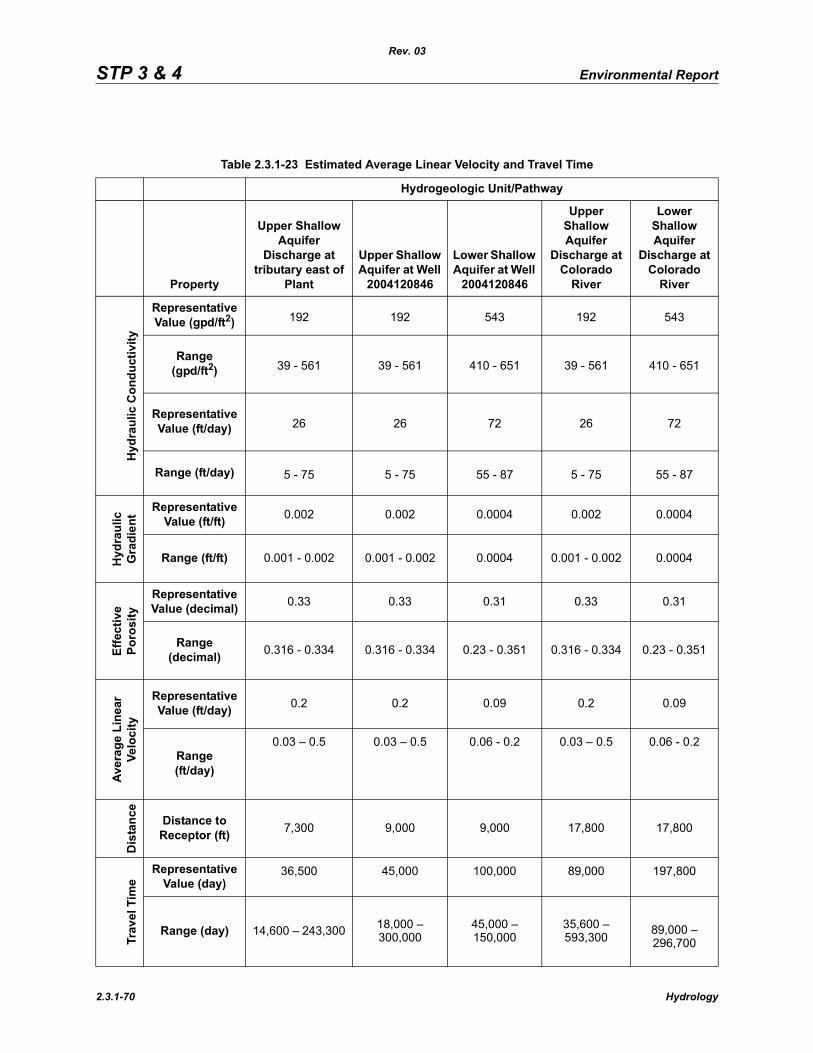
STP 3 & 4 Environmental Report
Rev. 03
Table 2.3.1-23 Estimated Average Linear Velocity and Travel Time
Hydrogeologic Unit/Pathway
Property
Upper Shallow Aquifer
Discharge at tributary east of
Plant
Upper Shallow Aquifer at Well
2004120846
Lower Shallow Aquifer at Well
2004120846
Upper Shallow Aquifer
Discharge at Colorado
River
Lower Shallow Aquifer
Discharge at Colorado
River
Hyd
raul
ic C
ondu
ctiv
ity
Representative Value (gpd/ft2) 192 192 543 192 543
Range(gpd/ft2) 39 - 561 39 - 561 410 - 651 39 - 561 410 - 651
Representative Value (ft/day) 26 26 72 26 72
Range (ft/day) 5 - 75 5 - 75 55 - 87 5 - 75 55 - 87
Hyd
raul
ic
Gra
dien
t Representative Value (ft/ft) 0.002 0.002 0.0004 0.002 0.0004
Range (ft/ft) 0.001 - 0.002 0.001 - 0.002 0.0004 0.001 - 0.002 0.0004
Effe
ctiv
ePo
rosi
ty
Representative Value (decimal) 0.33 0.33 0.31 0.33 0.31
Range(decimal) 0.316 - 0.334 0.316 - 0.334 0.23 - 0.351 0.316 - 0.334 0.23 - 0.351
Aver
age
Line
arVe
loci
ty
Representative Value (ft/day) 0.2 0.2 0.09 0.2 0.09
Range(ft/day)
0.03 – 0.5 0.03 – 0.5 0.06 - 0.2 0.03 – 0.5 0.06 - 0.2
Dis
tanc
e
Distance to Receptor (ft) 7,300 9,000 9,000 17,800 17,800
Trav
el T
ime
Representative Value (day)
36,500 45,000 100,000 89,000 197,800
Range (day) 14,600 – 243,300 18,000 – 300,000
45,000 – 150,000
35,600 – 593,300 89,000 –
296,700
2.3.1-70 Hydrology