Application of Orthogonal Frequency Division Multiplexing ...
description

Resource Allocation for Mobile Multiuser Orthogonal Frequency Division Multiplexing Systems
Prof. Brian L. EvansEmbedded Signal Processing Laboratory
Dept. of Electrical and Computer Engineering
The University of Texas at Austin
July 5, 2006
Featuring work by PhD students Zukang Shen (now at TI) and Ian WongCollaboration with Prof. Jeffrey G. Andrews and Prof. Robert W. Heath

2
Outline
Introduction Resource allocation in wireless systems Multiuser OFDM (MU-OFDM) Resource allocation in MU-OFDM
MU-OFDM resource allocation with proportional rates Near-optimal solution Low-complexity solution Real-time implementation
OFDM channel state information prediction Comparison of algorithms High-resolution joint estimation and prediction
Multiuser OFDM resource allocation using predicted channel state information

3
Resource Allocation in Wireless Systems
Wireless local area networks (WLAN) 54--108 Mbps Metropolitan area networks (WiMAX) ~10--100 Mbps Limited resources shared by multiple users
Transmit power Frequency bandwidth Transmission time Code resource Spatial antennas
Resource allocation impacts Power consumption User throughput System latency
user 4 user 5 user 6
user 1 user 2 user 3
time
frequency
code/spatial

4
Orthogonal Frequency Division Multiplexing
Adopted by many wireless communication standards IEEE 802.11a/g WLAN Digital Video Broadcasting – Terrestrial and Handheld
Broadband channel divided into narrowband subchannels Multipath resistant Receiver equalization simpler than single-carrier systems
Uses static time or frequency division multiple access
subcarrier
frequency
mag
nitu
de
channel
Bandwidth
OFDM Baseband Spectrum

5
Multiuser OFDM
Orthogonal frequency division multiple access (OFDMA) Adopted by IEEE 802.16a/d/e standards
802.16e: 1536 data subchannels with up to 40 users / sector
Users may transmit on different subcarriers at same time Inherits advantages of OFDM Exploits diversity among users
. . .User 1
User 2
frequencyBase Station(Subcarrier and power allocation)
User K

6
Exploiting Multiuser Diversity
Downlink multiuser OFDM Users share subchannels and
basestation transmit power Users only decode their own data
0 0.1 0.2 0.3 0.4 0.5-40
-30
-20
-10
0
10
Time (sec)
Channel g
ain
(dB
)
Rayleigh Fading Channel in a 10-user System
single user gainmax user gain
Resource Allocation
Static Adaptive
Users transmission
order
Pre-determined
Dynamically scheduled
Channel state
information
Not exploited
Wellexploited
SystemPerformance
Poor Good
7
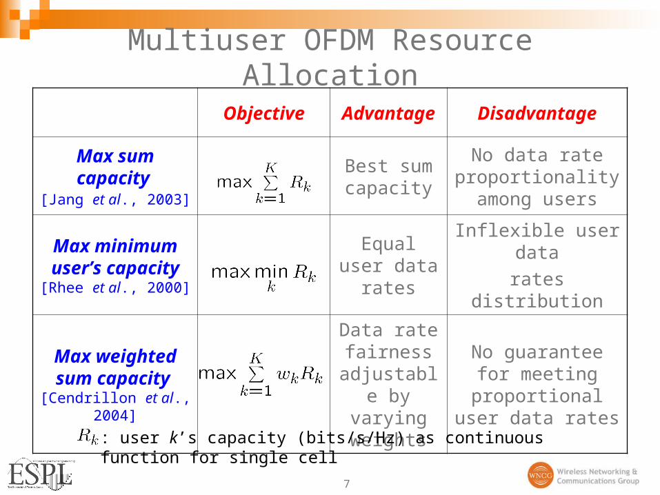
Multiuser OFDM Resource Allocation
Objective Advantage Disadvantage
Max sum capacity
[Jang et al., 2003]
Best sum capacity
No data rate proportionality among users
Max minimum user’s capacity [Rhee et al., 2000]
Equal user data rates
Inflexible user data
rates distribution
Max weightedsum capacity
[Cendrillon et al., 2004]
Data rate fairness
adjustable by varying
weights
No guarantee for meeting
proportional user data rates
: user k’s capacity (bits/s/Hz) as continuous function for single cell

8
Outline
Introduction Resource allocation in wireless systems Multiuser-OFDM (MU-OFDM) Resource allocation in MU-OFDM
MU-OFDM resource allocation with proportional rates Near-optimal solution Low-complexity solution Real-time implementation
OFDM channel state information prediction Comparison of algorithms High-resolution joint estimation and prediction
Multiuser OFDM resource allocation using predicted channel state information
9
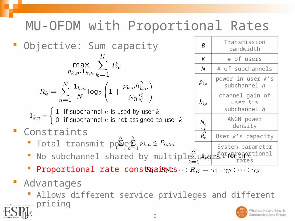
MU-OFDM with Proportional Rates Objective: Sum capacity
Constraints Total transmit power
No subchannel shared by multiple users
Proportional rate constraints
Advantages Allows different service privileges and different pricing
BTransmission
bandwidth
K # of users
N # of subchannels
pk,npower in user k’s
subchannel n
hk,nchannel gain of user k’s
subchannel n
N0 AWGN power density
Rk User k’s capacity
System parameter for proportional rates
10
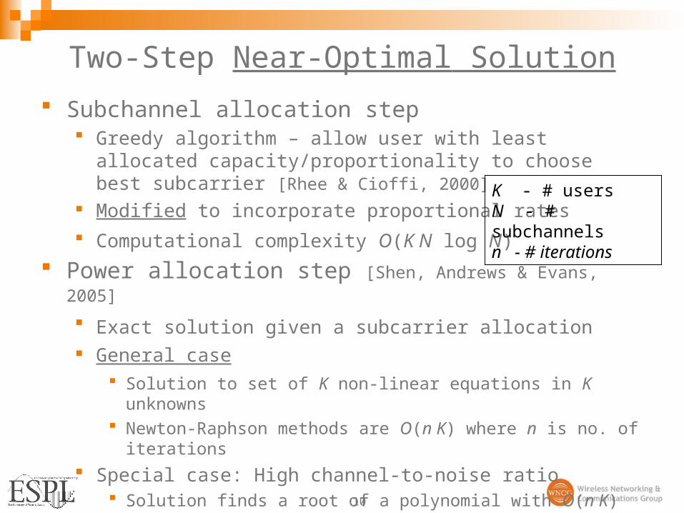
Two-Step Near-Optimal Solution
Subchannel allocation step Greedy algorithm – allow user with least
allocated capacity/proportionality to choosebest subcarrier [Rhee & Cioffi, 2000]
Modified to incorporate proportional rates Computational complexity O(K N log N)
Power allocation step [Shen, Andrews & Evans, 2005]
Exact solution given a subcarrier allocation General case
Solution to set of K non-linear equations in K unknowns Newton-Raphson methods are O(n K) where n is no. of iterations
Special case: High channel-to-noise ratio Solution finds a root of a polynomial with O(n K) complexity Typically 10 iterations in simulation
K - # usersN - # subchannelsn - # iterations

11
Lower Complexity Solution
In practical scenarios, rough proportionality is acceptable Key ideas to simplify Shen’s approach
[Wong, Shen, Andrews & Evans, 2004]
Relax strict proportionality constraint Require predetermined number of subchannels
to be assigned to simplify power allocation
Power allocation Solution to sparse set of linear equations Computational complexity O(K)
Advantages [Wong, Shen, Andrews & Evans, 2004]
Waives high channel-to-noise ratio assumption of Shen’s method Achieves higher capacity with lower complexity vs. Shen’s
method Maintains acceptable proportionality of user data rates
Example
108 7
4
12
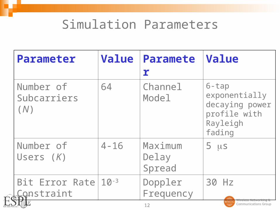
Simulation Parameters
Parameter Value Parameter Value
Number of Subcarriers (N)
64 Channel Model
6-tap exponentially decaying power profile with Rayleigh fading
Number of Users (K)
4-16 Maximum Delay Spread
5 s
Bit Error Rate Constraint
10-3 Doppler Frequency
30 Hz
13
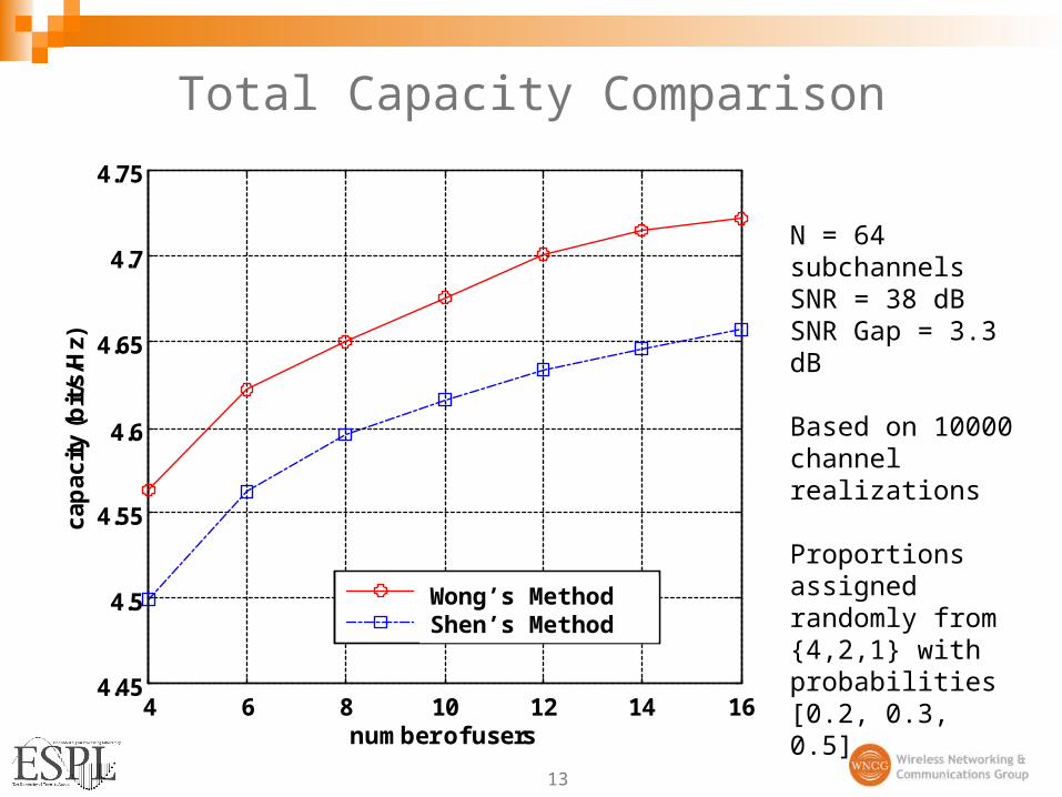
Total Capacity Comparison
4 6 8 10 12 14 164.45
4.5
4.55
4.6
4.65
4.7
4.75
number of users
cap
acity
(bit/
s/H
z)
Proposed Method
Shen's Method
N = 64 subchannelsSNR = 38 dBSNR Gap = 3.3 dB
Based on 10000 channel realizations
Proportions assigned randomly from {4,2,1} with probabilities[0.2, 0.3, 0.5]Wong’s Method
Shen’s Method

14
Proportionality Comparison
1 2 3 4 5 6 7 8 9 10 11 12 13 14 15 160
0.02
0.04
0.06
0.08
0.1
0.12
0.14
0.16
User Number (k)
No
rmal
ized
Ra
te P
rop
ort
ion
s
Proportions
Proposed Method
Shen's Method
Based on the 16-user case,10000 channelrealizations per user
Normalized rate proportions for three classes of users using proportions {4, 2, 1}
ProportionsWong’s MethodShen’s Method
15
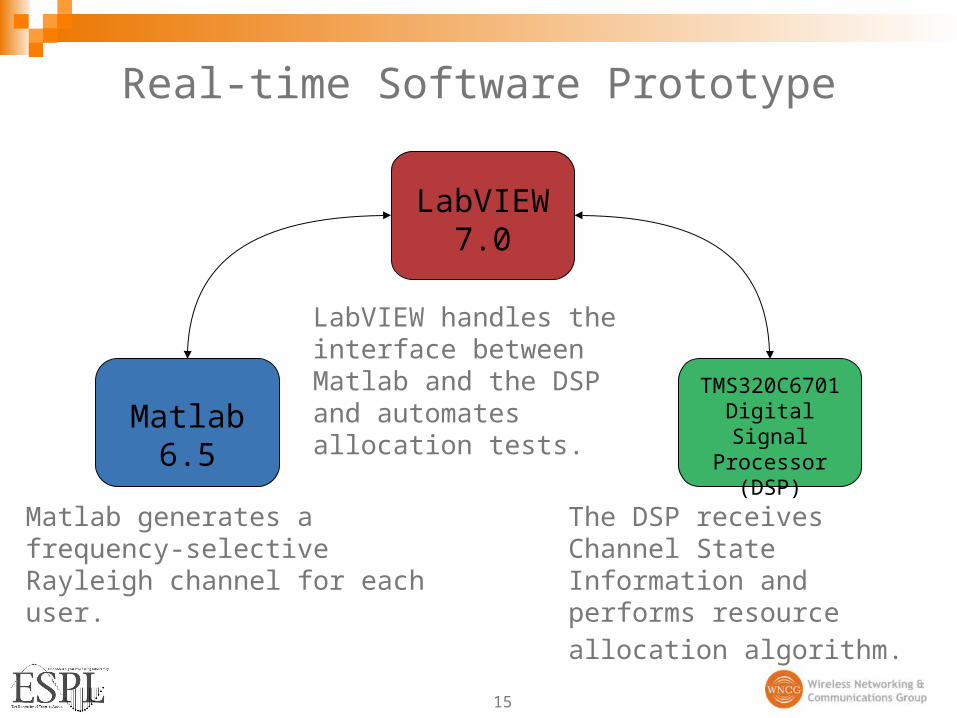
Real-time Software Prototype
Matlab generates a frequency-selective Rayleigh channel for each user.
Matlab 6.5
LabVIEW 7.0
TMS320C6701 Digital Signal
Processor (DSP)
The DSP receives Channel State Information and performs
resource allocation algorithm.
LabVIEW handles the interface between Matlab and the DSP and automates allocation tests.

16
Computational Complexity
2 4 6 8 10 12 14 160
1
2
3
4
5
6
7
8
9
10x 10
5 DSP Imlementation Clock cycle count
Number of users
Clo
ck c
ycle
s
Channel Allocation-shenPower Allocation-shen
Channel Allocation-wong
Power Allocation-wong
Total-shenTotal-wong Code developed
in floating point C
Run on 133 MHzTI TMS320C6701 DSP EVM board
22% average improvement

17
Memory Usage
Memory Type *Shen’s Method *Wong’s Method
Program
Memory
Subcarrier Allocation
1660 2024
Power Allocation
2480 1976
Total 4140 4000Data Memory
System Variables
8KN+4K
O(KN)
8KN+4K
O(KN)Subcarrier Allocation
4N+8K
O(N+K)
4N+12K
O(N+K)Power Allocation
4N+24K
O(N+K)
4N+28K
O(N+K)
* All values are in bytes

18
Performance Comparison Summary
Performance Criterion Shen’s Method Wong’s Method
Subcarrier Allocation Computational Complexity
O(K N log N) O(K N log N)
Power Allocation Computational Complexity
O(N + nK), n~9 O(N+K)
Memory Complexity O(NK) O(NK)Achieved Capacity High Higher
Adherence to Proportionality
Tight Loose
Assumptions on Subchannel SNR
High None
19
Outline
Introduction Resource allocation in wireless systems Multiuser-OFDM (MU-OFDM) Resource Allocation in MU-OFDM
MU-OFDM resource allocation with proportional rates Near-optimal solution Low-complexity solution Real-time implementation
OFDM channel state information prediction Comparison of algorithms High-resolution joint estimation and prediction
Multiuser OFDM resource allocation using predicted channel state information

20
Delayed Channel State Information
InternetBack haul
t=0: Mobile estimates channel and feeds this back to base stationt=ase station receives estimates, adapts transmission based on these t=0t=
Channel mismatch[Souryal & Pickholtz, 2001]
Higher BERLower bits/s/Hz
mobile
21
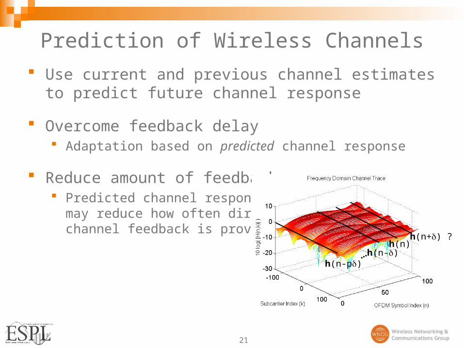
Prediction of Wireless Channels
Use current and previous channel estimates to predict future channel response
Overcome feedback delay Adaptation based on predicted channel response
Reduce amount of feedback Predicted channel response
may reduce how often directchannel feedback is provided
h(n-p)h(n-)
h(n)h(n+) ?
…

22
Related Work Prediction on each subcarrier [Forenza & Heath, 2002]
Each subcarrier treated as a narrowband autoregressive process [Duel-Hallen et al., 2000]
Prediction using pilot subcarriers [Sternad & Aronsson, 2003]
Used unbiased power prediction [Ekman, 2002]
Prediction on time-domain channel taps[Schafhuber & Matz, 2005]
Used adaptive prediction filters
… …
Pilot Subcarriers
Data Subcarriers
IFFT
Time-domain channel taps

23
OFDM Channel Prediction Comparison
Compared three approaches in unified framework[Wong, Forenza, Heath & Evans, 2004]
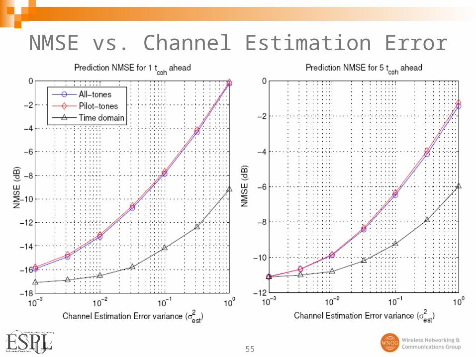
Analytical and numerical mean squared error comparison All-subcarrier and pilot-subcarrier methods have similar mean
squared error performance Time-domain prediction performs much better than the two other
frequency domain prediction methods
Complexity comparison All-subcarrier > Pilot-subcarrier ¸ Time-domain
NpNNNN tp and and

24
High-resolution OFDM Channel Prediction
Combined channel estimation and prediction[Wong & Evans, 2005]
Outperforms previous methods with similar order of computational complexity
Allows decoupling of computations between receiver and transmitter
High-resolution channel estimates available as aby-product of prediction algorithm

25
Deterministic Channel Model
Outdoor mobile macrocell scenario Far-field scatterer (plane wave assumption) Linear motion with constant velocity Small time window (a few wavelengths)
Channel model
Used in modeling and simulation ofwireless channels [Jakes 1974]
Used in ray-tracing channelcharacterization [Rappaport 2002]
n OFDM symbol indexk subchannel index
26
Prediction via 2-D Frequency Estimation
If we accurately estimate parameters in channel model, we could effectively extrapolate the fading process
Estimation and extrapolation period should be within time window where model parameters are stationary
Estimation of two-dimensional complex sinusoids in noise Well studied in radar, sonar, and other array signal processing
applications [Kay, 1988]
Many algorithms available, but are computationally intensive
27
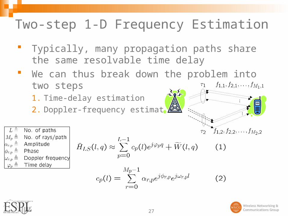
Two-step 1-D Frequency Estimation
Typically, many propagation paths share the same resolvable time delay
We can thus break down the problem into two steps1. Time-delay estimation
2. Doppler-frequency estimation
28
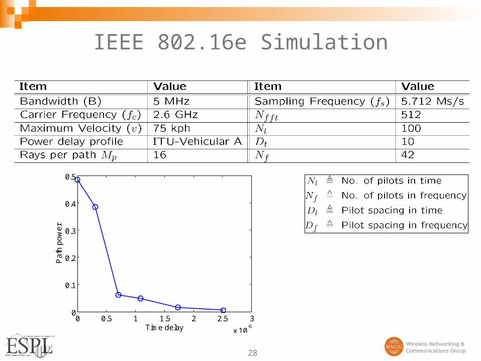
IEEE 802.16e Simulation
0 0.5 1 1.5 2 2.5 3
x 10-6
0
0.1
0.2
0.3
0.4
0.5
Time delay
Pa
th p
ow
er

29
Mean-square Error vs. SNR
10 15 20 25 30 35-50
-45
-40
-35
-30
-25
-20
-15
-10
SNR in dB
MS
E in
dB
ACRLB
CRLB
2-Step 1-Dimensional
Burg
Prediction 2 ahead
ACRLB – Asymptotic Cramer-Rao Lower Bound CRLB – Cramer-Rao Lower Bound
30
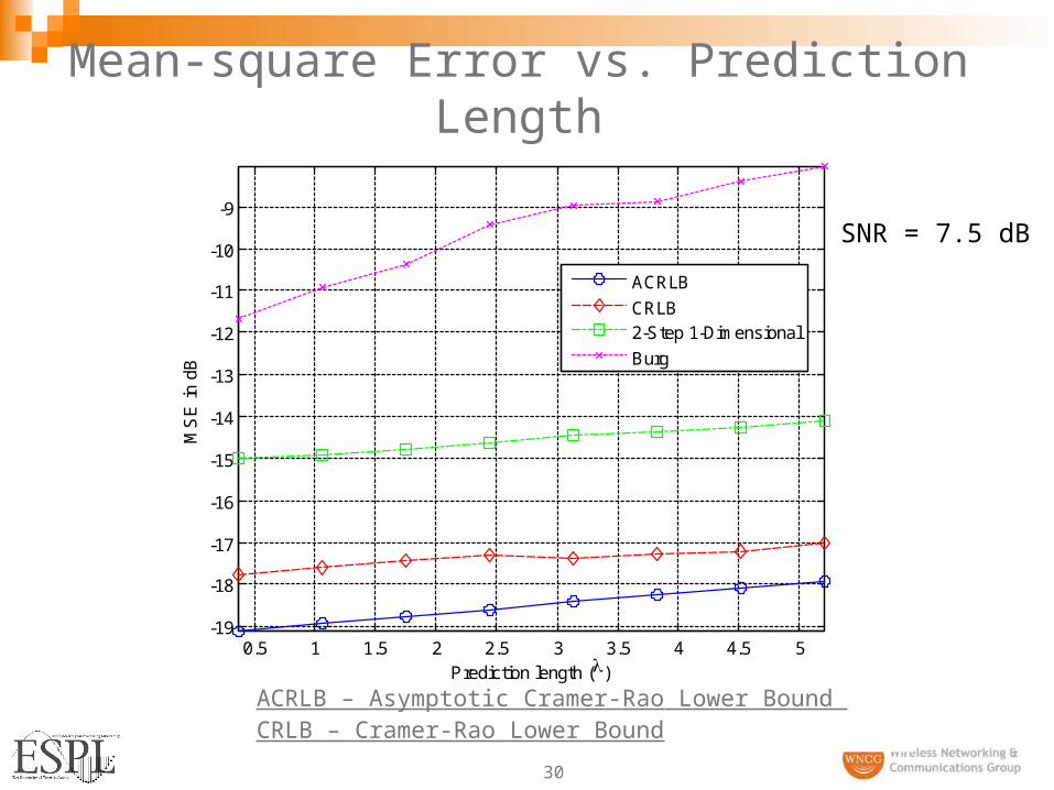
Mean-square Error vs. Prediction Length
SNR = 7.5 dB
ACRLB – Asymptotic Cramer-Rao Lower Bound CRLB – Cramer-Rao Lower Bound
0.5 1 1.5 2 2.5 3 3.5 4 4.5 5-19
-18
-17
-16
-15
-14
-13
-12
-11
-10
-9
Prediction length ()
MS
E in
dB
ACRLB
CRLB2-Step 1-Dimensional
Burg
31
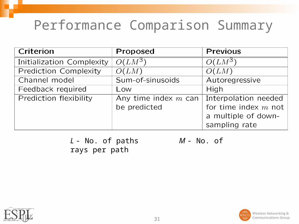
Performance Comparison Summary
L - No. of paths M - No. of rays per path

32
MU-OFDM Resource Allocation with Predicted Channel State Infomation (Future)
Combine MU-OFDM resource allocation with long-range channel prediction
Using the statistics of the channel prediction error, we can stochastically adapt to the channel Requires less channel feedback More resilient to channel feedback delay Improved overall throughput

33
Conclusion
Resource allocation for MU-OFDM with proportional rates Allows tradeoff between sum capacity and user rate “fairness” to
enable different service privileges and pricing Derived efficient algorithms to achieve similar performance with
lower complexity Prototyped system in a DSP, showing its promise for real-time
implementation
Channel prediction for OFDM systems Overcomes the detrimental effect of feedback delay Proposed high-performance OFDM channel prediction algorithms
with similar complexity Resource allocation using predicted channels is important for
practical realization of resource allocation in MU-OFDM

34
Director: Prof. Brian L. Evans http://www.ece.utexas.edu/~bevans/
WiMAX (OFDM) related research Algorithms for resource allocation in Multiuser OFDM Algorithms for OFDM channel estimation and prediction Key collaborators: Prof. Jeffrey Andrews and Prof. Robert Heath Key graduate students:
Embedded Signal Processing Laboratory
Youssof Mortazavi
Aditya Chopra
Hamood Rehman
Ian Wong
Marcel Nassar

35
Backup

36
Subchannel Allocation Modified method of [Rhee et al., 2000], but we keep the
assumption of equal power distribution on subchannels Initialization (Enforce zero initial conditions)
Set , for . Let
For to (Allocate best subchannel for each user) Find satisfying for all Let , and update
While (Iteratively give lowest rate user first choice) Find satisfying for all For the found , find satisfying for all For the found and , Let , and
update Back

37
Power Allocation for a Single User Optimal power distribution for user
Order Water-filling algorithm
How to find for
K # of users
N # of subchannels
pk,npower in user k’s nth assigned subchannel
Hk,n
Channel-to-noise ratio in user k’s nth assigned
subchannel
Nk# of subchannels
allocated to user k
Pk,totTotal power allocated to
user k
subchannels
Water-level

38
Power Allocation among Many Users Use proportional rate and total power constraints
Solve nonlinear system of K equations: /iteration Two special cases
Linear case: , closed-form solution High channel-to-noise ratio: and
where
Back

39
Comparison with Optimal Solution
-10 -5 0 5 100
0.5
1
1.5
2
2.5
3
3.5
10*log10(1/
2)
Ove
rall
capa
city
(bi
ts/s
/Hz)
optimal, E(ch1)/E(ch2)=1decoupled, E(ch1)/E(ch2)=1optimal, E(ch1)/E(ch2)=0.1decoupled, E(ch1)/E(ch2)=0.1optimal, E(ch1)/E(ch2)=10decoupled, E(ch1)/E(ch2)=10
Back

40
Comparison with Max-Min Capacity
8 10 12 14 160.2
0.4
0.6
0.8
1
1.2
1.4
1.6
Number of users K
Min
imum
Use
r's C
apac
ity (
bit/s
/Hz)
proposedmax-min:equal powerTDMA

41
Comparison with Max Sum Capacity
0 1 2 3 4 5 6 76
7
8
9
10
Fairness Index m
Erg
odic
Sum
Cap
acity
(bits
/s/H
z)
max sum capacitysingle user (higher SNR)proposedstatic TDMAsingle user (lower SNR)
1 2 3 4 5 6 7 80
0.2
0.4
0.6
0.8
Nor
mal
ized
Erg
odic
Cap
acity
Per
Use
rUser Index k
ideal, m=3proposed m=3max sum capacitystatic TDMA

42
Summary of Shen’s Contribution
Adaptive resource allocation in multiuser OFDM systems Maximize sum capacity Enforce proportional user data rates
Low complexity near-optimal resource allocation algorithm Subchannel allocation assuming equal power on all subchannels Optimal power distribution for a single user Optimal power distribution among many users with proportionality
Advantages Evaluate tradeoff between sum capacity and user data rate fairness Fill the gap of max sum capacity and max-min capacity Achieve flexible data rate distribution among users Allow different service privileges and pricing

43
Wong’s 4-Step Approach
1. Determine number of subcarriers Nk for each user
2. Assign subcarriers to each user to give rough proportionality
3. Assign total power Pk for each user to maximize capacity
4. Assign the powers pk,n for each user’s subcarriers (waterfilling)
O(K)
O(N)
O(KNlogN)
O(K)
44
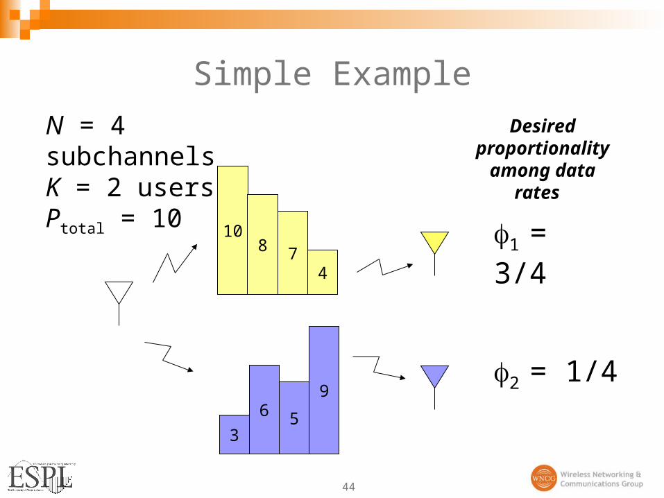
Simple Example
2 = 1/4
1 = 3/4
3
6 5
9
N = 4 subchannelsK = 2 usersPtotal = 10
108 7
4
Desired proportionality
among data rates

45
Step 1: # of Subcarriers/User
108 7
4
3
6 5
9
Nk
3
1
1 2 3 4
2 = 1/4
1 = 3/4
N = 4 subchannelsK = 2 usersPtotal = 10

46
Step 2: Subcarrier Assignment
Nk
3/4 3
1/4 11 2 3 4
3
6 5
9
1 2 3 4
Rk
log2(1+2.5*10)=4.70
log2(1+2.5*7)=4.21
108
478
47
47
1010log2(1+2.5*8)=4.39
Rtot
13.3
9log2(1+2.5*9)=4.55 4.55
4
108
10108 7
3
6 5

47
Step 3: Power per user
1 2 3 4
10108 7
9
P1 = 7.66 P2 = 2.34
N = 4 subchannels; K = 2 users; Ptotal = 10 Back

48
Step 4: Power per subcarrier
Nk
3/4 3
1/4 1
p1,1= 2.58 p1,2= 2.55p1,3= 2.53 p2,1= 2.34 Data Rates:R1 = log2(1 + 2.58*10) + log2(1 + 2.55*8)
+ log2(1 + 2.53*7) = 13.39008R2 = log2(1+ 2.34*9) = 4.46336
P1 = 7.66 P2 = 2.34
1 2 3 4
10108 7
9
• Waterfilling across subcarriers for each user
Back

49
Comb pilot pattern
Least-squares channel estimates
Pilot-based Transmission
t
f …
Dt
Df

50
Design prediction filter for each of the Nd data subcarriers
Mean-square error
Prediction over all the subcarriers

51
Design filter on the Npilot pilot subcarriers only Less computation and storage needed
Npilot << Nd (e.g. Npilot = 8; Nd = 192 for 802.16e OFDM)
Use the same prediction filter for the data subcarriers nearest to the pilot carrier
Prediction over the pilot subcarriers
… …
Pilot Subcarriers
Data Subcarriers

52
Design filter on Nt · Npilot time-domain channel taps Channel estimates typically available only in freq. domain IFFT required to compute time-domain channel taps
MSE:
Prediction on time-domain channel taps

53
Parameter Value Parameter Value
N 256 Bandwidth 5 MHz
Guard Carriers (7)
[0-27] &
[201:256]
Fcarrier 2600 MHz
Channel Model ETSI Vehicular A Mobile Velocity 75 kmph
Prediction Order
75 Downsampling rate 25
(4*fd)
Simulation Parameters (IEEE 802.16e)

54
Prediction Snapshot
55
NMSE vs. Channel Estimation Error

56
NMSE vs. Prediction Horizon

57
Step 1 – Time-delay estimation
Estimate autocorrelation function using the modified covariance averaging method [Stoica & Moses, 1997]
Estimate the number of paths L using minimum description length rule [Xu, Roy, & Kailath, 1994]
Estimate the time delays using Estimation of Signal Parameters via Rotational Invariance Techniques (ESPRIT) [Roy & Kailath, 1989]
Estimate the amplitudes cp(l) using least-squares Discrete Fourier Transform of these amplitudes could be used to
estimate channel More accurate than conventional approaches, and similar to parametric
channel estimation method in [Yang, et al., 2001]

58
Step 2 – Doppler Frequency Estimation
Using complex amplitudes cp(l) estimated from Step 1 as the left hand side for (2), we determine the rest of the parameters
Similar steps as Step 1 can be applied for the parameter estimation for each path p
Using the estimated parameters, predict channel as
59
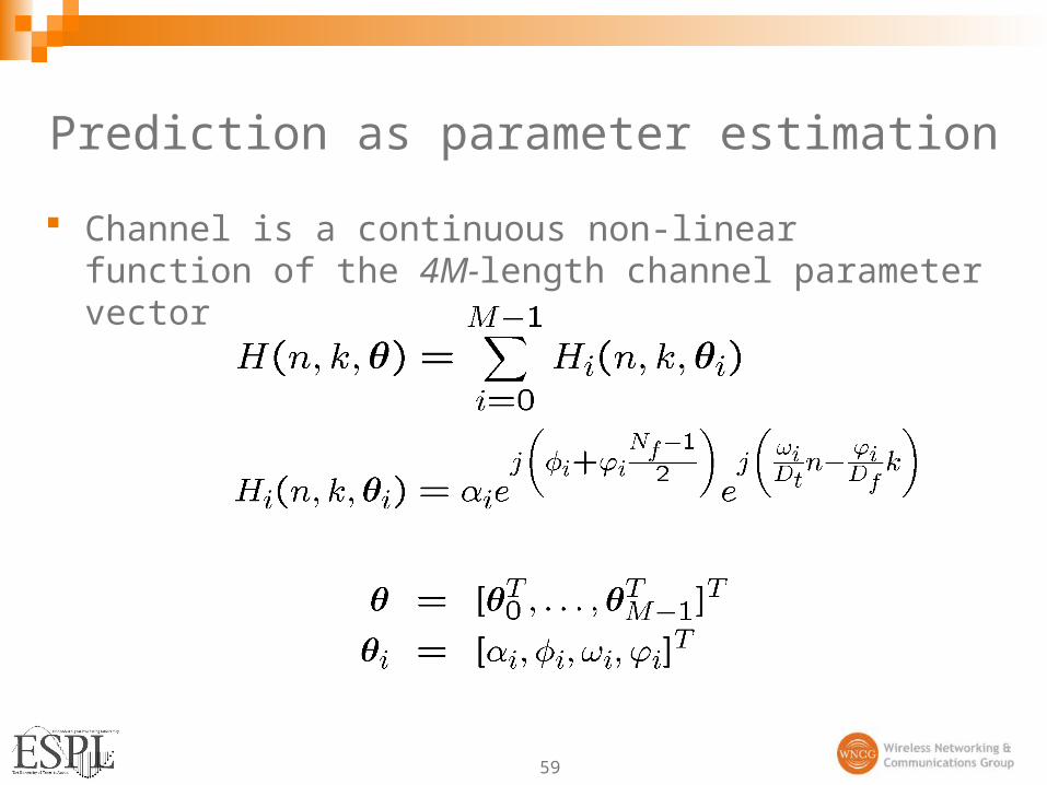
Prediction as parameter estimation
Channel is a continuous non-linear function of the 4M-length channel parameter vector

60
Cramer-Rao Lower Bound (CRLB)

61
Closed-form expression for asymptotic CRLB
Using large-sample limit of CRLB matrix for general 2-D complex sinusoidal parameter estimation [Mitra & Stoica, 2002]
Much simpler expression Achievable by maximum-likelihood and nonlinear least-squares
methods Monte-Carlo numerical evaluations not necessary

62
Insights from the MSE expression
Linear increase with 2 and M Dense multipath channel environments are the hardest to predict [Teal, 2002]
Quadratic increase in n and |k| with f and estimation error variances Emphasizes the importance of estimating these accurately
Nt, Nf, Dt and Df should be chosen as large as possible to decrease the MSE bound
Amplitude & phase error variance
Doppler frequency & phase cross covariance
Doppler frequency error variance
Time-delay & phase cross covariance
Time-delay error variance
63
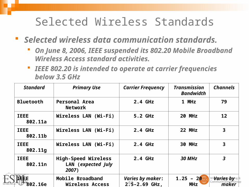
Selected Wireless Standards
Selected wireless data communication standards. On June 8, 2006, IEEE suspended its 802.20 Mobile
Broadband Wireless Access standard activities. IEEE 802.20 is intended to operate at carrier frequencies
below 3.5 GHzStandard Primary Use Carrier Frequency Transmission
BandwidthChannels
Bluetooth Personal Area Network 2.4 GHz 1 MHz 79
IEEE 802.11a Wireless LAN (Wi-Fi) 5.2 GHz 20 MHz 12
IEEE 802.11b Wireless LAN (Wi-Fi) 2.4 GHz 22 MHz 3
IEEE 802.11g Wireless LAN (Wi-Fi) 2.4 GHz 30 MHz 3
IEEE 802.11n High-Speed Wireless LAN (expected July 2007)
2.4 GHz 30 MHz 3
IEEE 802.16e Mobile Broadband Wireless Access(Wi-Max)
Varies by maker:2.5–2.69 GHz,
3.3–3.8 GHz, or5.725–5.850 GHz
1.25 – 20 MHz Varies by maker
7 – 400