Orthogonal Frequency Division Multiplexing

PhD First Progress Seminar Report

Submitted in the partial fulfillment of the requirements

for the degree of

Doctor of philosophy

by

Santosh V Jadhav

Roll No. 02407802

under the guidance of

Prof. Vikram M Gadre

Department of Electrical Engineering

Indian Institute of Technology, Bombay

August 2003

1

Acknowledgement I would like to express my sincere gratitude to my guide, Prof. Dr. Vikram M

Gadre for his help and guidance during the course of my first progress seminar.

Thanks to Dr K L Asanare, Director, FAMT for his continuous encouragement

and support. Also thanks to mathematics professor Dr Ch V Ramanamurthy for

helping me during this seminar preparation.

Santosh V Jadhav

August 2003

2

Contents Abstract

1. Single carrier to multi-carrier and multi-carrier to OFDM

1.1 Single Carrier modulation

1.2 Multicarrier approach

1.3 Orthogonal Frequency Division Multiplexing

2. Band-Limited Orthogonal Signals for Multichannel Data Transmission 2.1 Need of orthogonality in time-functions

2.2 Synthesis of OFDM signals for multichannel data transmission

2.2.1 Orthogonal multiplexing using band-limited signals

2.2.2 Transmission filter characteristics

2.3. Receiver structure for multichannel orthogonal signal

3. OFDM: FFT Based Approach

3.1 The Discrete-Time Model

3.2 Modulation of OFDM data using IDFT

3.3 Orthogonality

3.4 The cyclic prefix

3.5 Demodulation using the DFT

4. The Downsides of OFDM

5. Future Directions

References

1

2

2

2

4

5

5

9

10

16

24

27

27

29

31

32

33

35

38

39

3

Abstract Orthogonal frequency division multiplexing (OFDM) is used for transmitting a

number of data messages simultaneously through a linear band-limited transmission

medium at a maximum data rate without interchannel and intersymbol interferences.

Chapter-1 gives an idea about how OFDM is evolved from single carrier and

multicarrier modulation schemes. Chapter-2 discusses a general method for

synthesizing an infinite number of classes of band-limited orthogonal time functions

in a limited frequency band. Stated in practical terms, the method permits the

synthesis of a large class of practical transmitting filter characteristics for an

arbitrarily given amplitude characteristics of the transmission medium. Chapter-3

explains how Fourier transform data communication system acts as a realization of

OFDM in which discrete Fourier transform (DFT) and inverse DFT are computed as

part of the modulation and demodulation processes respectively. Chapter-4 and 5

gives drawbacks of OFDM and how endless appetite to achieve capacity, maximum

bit rate and minimum bit error rate (BER) gives rise to the future research scopes in

this field.

4

Chapter 1.

Single carrier to multi-carrier and multi-carrier to OFDM

Nonideal linear filter channels introduce intersymbol interference (ISI), which

degrades performance compared with the ideal channel. The degree of performance

degradation depends on the frequency-response characteristics. Furthermore, the

complexity of the receiver increases as the span of the ISI increases. Given a

particular channel characteristic, the communication system designer must decide

how to efficiently utilize the available channel bandwidth in order to transmit the

information reliably within the transmitter power constraint and receiver complexity

constraints.

1.1 Single Carrier modulation : For a nonideal linear filter channel, one option is to employ a single carrier (SC)

modulation system in which the information sequence is transmitted serially at some

specified rate R symbols/s. In such a channel, the time dispersion is generally much

greater than the symbol rate, and, hence, ISI results from the non-ideal frequency-

response characteristics of the channel. If the level of interference is sufficient to

noticeably deteriorate the radio link, then an equalizer is used at the receiver to

remove the effects of ISI.

1.2 Multicarrier approach : An alternative approach to the design of a bandwidth-efficient communication

system in the presence of channel distortion is to subdivide the available channel

bandwidth into a number of subchannels, such that each subchannel is nearly ideal.

To elaborate, suppose that H(f) is the frequency response of a non-ideal, band-limited

channel with a bandwidth B, and that the power spectral density of the additive

Gaussian noise is φnn(f). Then, divide the bandwidth B into N=B/∆f subbands of width

∆f, where ∆f is chosen sufficiently small that |H(f)|2/φnn(f) is approximately a constant

within each subband. Furthermore, we select the transmitted signal power to be

distributed in frequency as P(f), subject to the constraint that

5

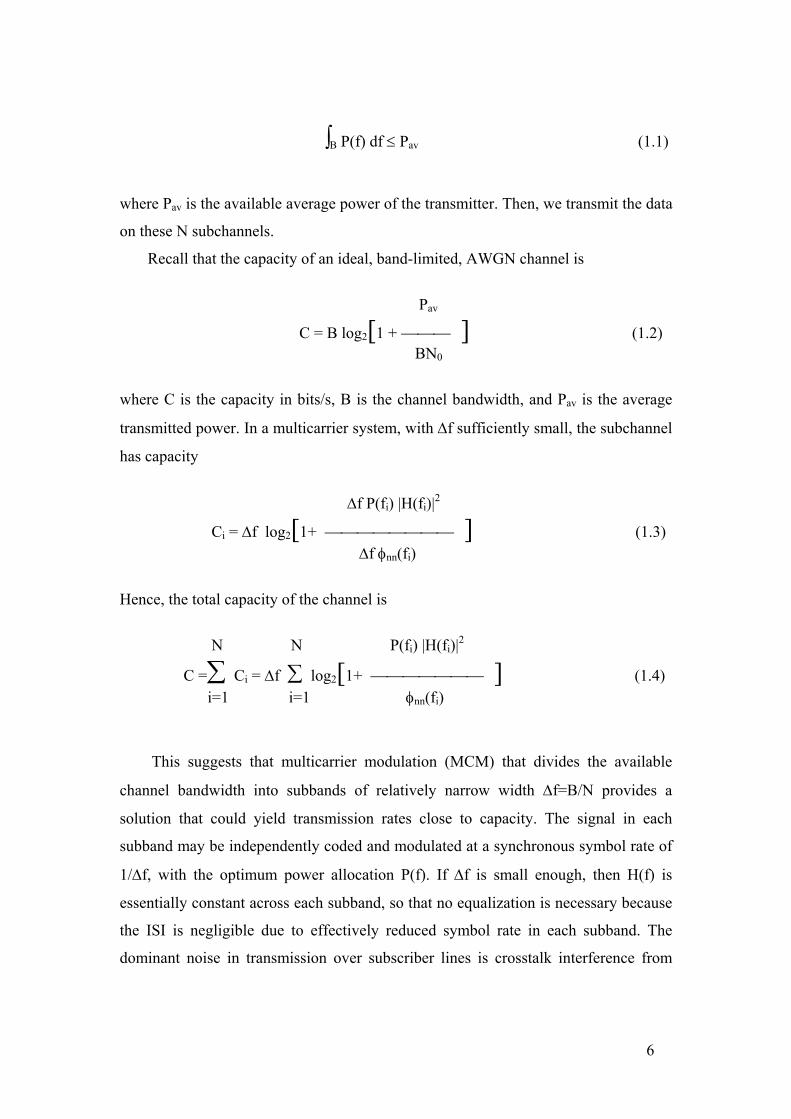
∫B P(f) df ≤ Pav (1.1)

where Pav is the available average power of the transmitter. Then, we transmit the data

on these N subchannels.

Recall that the capacity of an ideal, band-limited, AWGN channel is

Pav

C = B log2[1 + ] (1.2) BN0

where C is the capacity in bits/s, B is the channel bandwidth, and Pav is the average

transmitted power. In a multicarrier system, with ∆f sufficiently small, the subchannel

has capacity

∆f P(fi) |H(fi)|2

Ci = ∆f log2[1+ ] (1.3) ∆f φnn(fi)

Hence, the total capacity of the channel is

N N P(fi) |H(fi)|2

C =∑ Ci = ∆f ∑ log2[1+ ] (1.4) i=1 i=1 φnn(fi)

This suggests that multicarrier modulation (MCM) that divides the available

channel bandwidth into subbands of relatively narrow width ∆f=B/N provides a

solution that could yield transmission rates close to capacity. The signal in each

subband may be independently coded and modulated at a synchronous symbol rate of

1/∆f, with the optimum power allocation P(f). If ∆f is small enough, then H(f) is

essentially constant across each subband, so that no equalization is necessary because

the ISI is negligible due to effectively reduced symbol rate in each subband. The

dominant noise in transmission over subscriber lines is crosstalk interference from

6

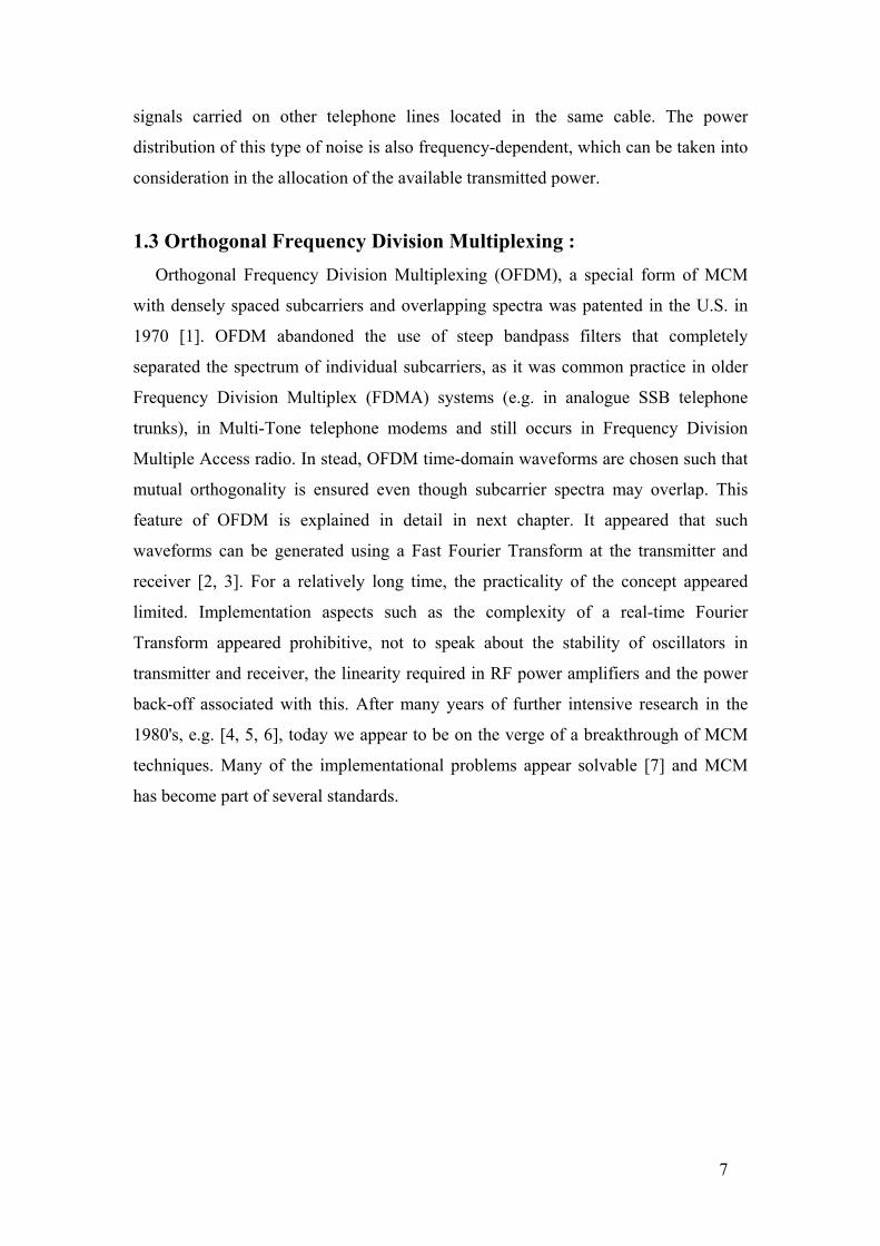
signals carried on other telephone lines located in the same cable. The power

distribution of this type of noise is also frequency-dependent, which can be taken into

consideration in the allocation of the available transmitted power.

1.3 Orthogonal Frequency Division Multiplexing : Orthogonal Frequency Division Multiplexing (OFDM), a special form of MCM

with densely spaced subcarriers and overlapping spectra was patented in the U.S. in

1970 [1]. OFDM abandoned the use of steep bandpass filters that completely

separated the spectrum of individual subcarriers, as it was common practice in older

Frequency Division Multiplex (FDMA) systems (e.g. in analogue SSB telephone

trunks), in Multi-Tone telephone modems and still occurs in Frequency Division

Multiple Access radio. In stead, OFDM time-domain waveforms are chosen such that

mutual orthogonality is ensured even though subcarrier spectra may overlap. This

feature of OFDM is explained in detail in next chapter. It appeared that such

waveforms can be generated using a Fast Fourier Transform at the transmitter and

receiver [2, 3]. For a relatively long time, the practicality of the concept appeared

limited. Implementation aspects such as the complexity of a real-time Fourier

Transform appeared prohibitive, not to speak about the stability of oscillators in

transmitter and receiver, the linearity required in RF power amplifiers and the power

back-off associated with this. After many years of further intensive research in the

1980's, e.g. [4, 5, 6], today we appear to be on the verge of a breakthrough of MCM

techniques. Many of the implementational problems appear solvable [7] and MCM

has become part of several standards.

7

Chapter 2.

Band-Limited Orthogonal Signals for Multichannel Data

Transmission

2.1 Need of orthogonality in time-functions :

Consider a set of orthogonal functions φ1(θ), φ2(θ), … , φi(θ) in the region

–½ ≤ θ ≤ +½. From the definition of orthogonal functions[8] follows-

+½

∫ φl(θ) φm(θ) dθ = K for l = m (2.1) –½ = 0 for l ≠ m

K is assumed to normalized to 1.

If the functions φ(θ) are multiplied by 1 or 0 and added, one obtains a function f(θ).

For example, if φ1(θ), φ2(θ), φ3(θ) are multiplied by 1 and all other φ(θ) by 0, the

result is the function-

f(θ) = φ1(θ) + φ2(θ) + φ3(θ) (2.2)

Because of the orthogonality of the functions φ(θ) one may readily decompose f(θ)

to determine which of the functions φ1(θ) … φi(θ) have been multiplied by 1.

Application of (2.1) yields-

+½

∫ f(θ) φl(θ) dθ = 1 for l =1,2,3 (2.3) –½ = 0 for l =4,5,…

Figure 2.1 shows a diagram of a communication system which uses the normalized

orthogonal system of sine and cosine functions 1, √2Sin 2kπθ, √2Cos 2kπθ; θ = t/τ,

k=1,2,… The first five of these functions are shown in figure 2.2. Assume that the

five digits character 11001 is to be transmitted. The switches (multipliers) in the

transmitter let through 1, √2Sin 2πθ and √2Cos 4πθ, but not √2Cos 2πθ and

√2Sin 4πθ. The adder adds the voltages and yield –

f(θ) = 1 + √2Sin 2πθ + √2Cos 4πθ (2.4)

8

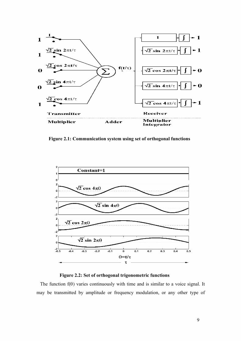
Figure 2.1: Communication system using set of orthogonal functions

Figure 2.2: Set of orthogonal trigonometric functions

The function f(θ) varies continuously with time and is similar to a voice signal. It

may be transmitted by amplitude or frequency modulation, or any other type of

9

modulation suitable for the transmission of continuously varying time functions. In

the receiver f(θ) is multiplied by the same five functions which were used in the

transmitted, the integral over the period τ is taken and the character 11001 multiplied

by τ is recovered

+½

τ ∫ f(θ)(1) dθ = τ –½

+½

τ ∫ f(θ) √2Sin 2πθ dθ = τ –½

+½

τ ∫ f(θ) √2Cos 2πθ dθ = 0 –½

+½

τ ∫ f(θ) √2Sin 4πθ dθ = 0 –½

+½

τ ∫ f(θ) √2Cos 4πθ dθ = τ –½

Here only trigonometric functions are considered but there is no difficulty other than

computational in applying other sets of orthogonal functions.

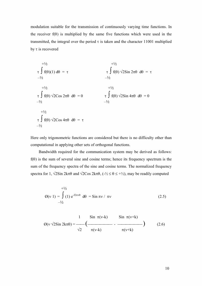
Bandwidth required for the communication system may be derived as follows:

f(θ) is the sum of several sine and cosine terms; hence its frequency spectrum is the

sum of the frequency spectra of the sine and cosine terms. The normalized frequency

spectra for 1, √2Sin 2kπθ and √2Cos 2kπθ, (-½ ≤ θ ≤ +½), may be readily computed

+½

Ø(ν 1) = ∫ (1) e-J2πνθ dθ = Sin πν / πν (2.5) –½ 1 Sin π(ν-k) Sin π(ν+k)

Ø(ν √2Sin 2kπθ) = ( - ) (2.6) √2 π(ν-k) π(ν+k)

10

1 Sin π(ν-k) Sin π(ν+k)

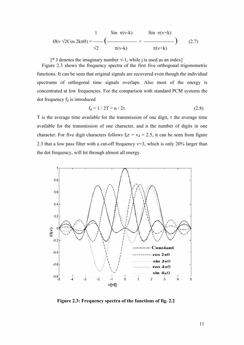
Ø(ν √2Cos 2kπθ) = ( + ) (2.7) √2 π(ν-k) π(ν+k) [* J denotes the imaginary number √-1, while j is used as an index] Figure 2.3 shows the frequency spectra of the first five orthogonal trigonometric

functions. It can be seen that original signals are recovered even though the individual

spectrums of orthogonal time signals overlaps. Also most of the energy is

concentrated at low frequencies. For the comparison with standard PCM systems the

dot frequency fd is introduced

fd = 1 / 2T = n / 2τ (2.8)

T is the average time available for the transmission of one digit, τ the average time

available for the transmission of one character, and n the number of digits in one

character. For five digit characters follows fdτ = νd = 2.5, it can be seen from figure

2.3 that a low pass filter with a cut-off frequency ν=3, which is only 20% larger than

the dot frequency, will let through almost all energy.

Figure 2.3: Frequency spectra of the functions of fig. 2.2

11

2.2 Synthesis of OFDM signals for multichannel data transmission : In this section it is shown that by using a new class of band-limited orthogonal

signals, the channels can transmit through a linear band-limited transmission medium

at a maximum possible data rate without interchannel and intersymbol interferences.

A general method is given for synthesizing an infinite number of classes of band-

limited orthogonal time-functions in a limited frequency band. This method permits

one to synthesize a large class of transmitting filter characteristics for arbitrarily given

amplitude and phase characteristics of the transmission medium. The synthesis

procedure is convenient. Furthermore, the amplitude and the phase characteristics of

the transmitting filters can be synthesized independently, i.e., the amplitude

characteristics need not be altered when the phase characteristics are changed, and

vice versa. The system can be used to transmit not only binary digits or m-ary digits,

but also real numbers, such as time samples of analog information sources. As will be

shown, the system satisfies the following requirements.

(i) The transmitting filters have gradual cutoff amplitude characteristics.

Perpendicular cutoffs and linear phases are not required.

(ii) The data rate per channel is 2fs bauds, where fs is the center frequency difference

between two adjacent channels. Overall data rate of the system is [N/(N+1)] Rmax,

where N is the total number of channels and Rmax, which equals two times the overall

baseband bandwidth, is the Nyquist rate for which unrealizable rectangular filters with

perpendicular cutoffs and linear phases are required. Thus, as N increases, the overall

data rate of the system approaches the theoretical maximum rate Rmax, yet rectangular

filtering is not required.

(iii) When transmitting filters are designed for an arbitrary given amplitude

characteristic of the transmission medium, the received signals remain orthogonal for

all phase characteristics of the transmission medium. Thus, the system (orthogonal

transmission plus adaptive correlation reception) eliminates interchannel and

intersymbol interferences for all phase characteristics of the transmission medium.

(iv) The distance in signal space between any two sets of received signals is the same

as if the signals of each channel were transmitted through an independent medium and

intersymbol interference in each channel were eliminated by reducing data rate. The

same distance protection is therefore provided against channel noise (impulse and

12

Gaussian noise). For instance, for band-limited white Gaussian noise, the receiver

receives each of the overlapping signals with the same probability of error as if only

that signal were transmitted. The distances in the signals space are also independent of

the phase characteristics of the transmitting filters and the transmission medium.

(v) When signaling intervals of different channels are not synchronized, at least half

of the channels can transmit simultaneously without interchannel and intersymbol

interference.

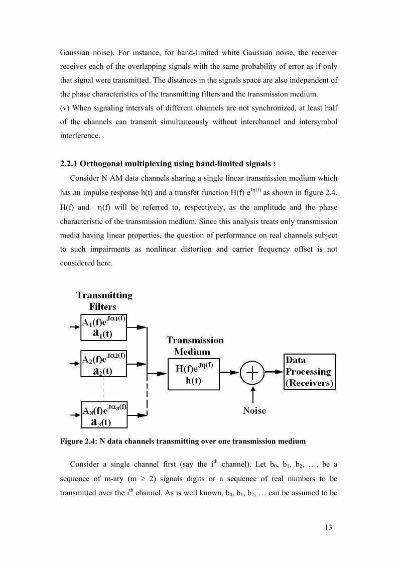
2.2.1 Orthogonal multiplexing using band-limited signals :

Consider N AM data channels sharing a single linear transmission medium which

has an impulse response h(t) and a transfer function H(f) eJη(f) as shown in figure 2.4.

H(f) and η(f) will be referred to, respectively, as the amplitude and the phase

characteristic of the transmission medium. Since this analysis treats only transmission

media having linear properties, the question of performance on real channels subject

to such impairments as nonlinear distortion and carrier frequency offset is not

considered here.

Figure 2.4: N data channels transmitting over one transmission medium

Consider a single channel first (say the ith channel). Let b0, b1, b2, …, be a

sequence of m-ary (m ≥ 2) signals digits or a sequence of real numbers to be

transmitted over the ith channel. As is well known, b0, b1, b2, … can be assumed to be

13

represented by impulses with proportional heights. These impulses are applied to the

ith transmitting filter at the rate of one impulse every T seconds (data rate per channel

equals 1/T bauds). Let ai(t) be the impulse response of the ith transmitting filter, then

the ith transmitting filter transmits a sequence of signals as

b0 ai(t) + b1 ai(t-T) + b2 ai(t-2T) + …, (2.9)

The received signals at the output of the transmission medium are

b0 ui(t) + b1 ui(t-T) + b2 ui(t-2T) + …, (2.10)

where

+∞

ui(t) = ∫ h(t-τ) ai(τ) dτ (2.11) –∞

These received signals overlap in time, but they are orthogonal if

+∞

∫ ui(t) ui(t-kT) dt = 0, k = ±1, ±2, … (2.12) -∞

As is well known, orthogonal signals can be separated at the receiver by correlation

techniques; hence, intersymbol interference in the ith channel can be eliminated if

(2.12) is satisfied.

Next consider interchannel interference. Let c0, c1, c2, … be the m-ary signal digits

or real numbers transmitted over the jth channel which has impulse response aj(t). It

has been assumed that the channels transmit at the same data rate and that the

signaling intervals of different channels are synchronized, hence the jth transmitting

filter transmits a sequence of signals,

c0 aj(t) + c1 aj(t-T) + c2 aj(t-2T) + …, (2.13)

14

The received signals at the output of the transmission medium are

c0 uj(t) + c1 uj(t-T) + c2 uj(t-2T) + …, (2.14)

These received signals overlap with the received signals of the ith channel, but they

are mutually orthogonal (no interchannel interference) if

+∞

∫ ui(t) uj(t-kT) dt = 0, k = 0, ±1, ±2, … (2.15) -∞

Thus, intersymbol and interchannel interferences can be simultaneously eliminated if

the transmitting filters can be designed (i.e., if the transmitted signals can be

designed) such that (2.12) is satisfied for all i and (2.15) is satisfied for all i and j

(i ≠ j).

Denote Ui(f) eJµi(f) as the Fourier transform of ui(t). One can rewrite (2.12) as

+∞

∫ U i 2(f) e-J2πfkT df = 0, k = ±1, ±2, … i=1,2, … ,N, (2.16)

-∞

and rewrite (2.15) as

+∞

∫Ui(f) eJµi(f) Uj(f) e-Jµj(f) e-J2πfkT df = 0, -∞ k = 0, ±1, ±2, … i,j =1,2, … ,N, i ≠ j (2.17)

Let Ai(f) eJαi(f) be the Fourier transform of ai(t). The transfer function of the

transmission medium is H(f) eJη(f). Equation (2.16) becomes

+∞

∫ Ai2(f)H2(f) e-J2πfkT df = 0, k = ±1, ±2,… i=1,2, … ,N, (2.18)

-∞

15

alternatively

+∞

∫ Ai2(f)H2(f) [Cos 2πfkT – J Sin 2πfkT ] df = 0,

-∞ k = ±1, ±2,… i=1,2, … ,N,

+∞

∫ [Ai2(f)H2(f) Cos 2πfkT df– J Ai

2(f)H2(f) Sin 2πfkT ] df = 0, -∞ k = ±1, ±2,… i=1,2, … ,N,

+∞ +∞

∫ Ai2(f)H2(f) Cos 2πfkT df– J ∫ Ai

2(f)H2(f) Sin 2πfkT df = 0, -∞ -∞ k = ±1, ±2,… i=1,2, … ,N,

Here imaginary part of LHS of above equation is ZERO, as it is the integration of odd

symmetric function (Ai2(f)H2(f) Sin 2πfkT) from -∞ to +∞.

+∞

∴ ∫ Ai2(f)H2(f) Cos 2πfkT df = 0, k = ±1, ±2,… i=1,2, … ,N,

-∞ As function under above integration (Ai

2(f)H2(f) Cos 2πfkT) is even, this equation can

be written as –

∞

∫ Ai2(f)H2(f) Cos 2πfkT df = 0, k = 1, 2,… i=1,2, … ,N, (2.19)

0

and equation (2.17) becomes

16

+∞

∫Ai(f)Aj(f) H2(f) eJ[αi(f) - αj(f) - 2πfkT] df = 0, -∞ k = 0, ±1, ±2, … i,j =1,2,… ,N, i ≠ j (2.20)

This equation (2.17) can be written as

+∞

∫Ai(f)Aj (f) H2(f) Cos[αi(f) - αj(f) - 2πfkT] df + -∞ +∞

J ∫Ai(f)Aj(f) H2(f) Sin[αi(f) - αj(f) - 2πfkT] df = 0 -∞ k = 0, ±1, ±2, … i,j =1,2, … ,N, i ≠ j

Here imaginary part of LHS of above equation is ZERO, as it is the integration of odd

symmetric function (Ai(f) Aj(f) H2(f) Sin[αi(f)-αj(f)-2πfkT]) from -∞ to +∞. Applying

symmetry arithmetic and trigonometric identity to real part we have,

∞

∫Ai(f)Aj (f) H2(f) Cos[αi(f) - αj(f)].Cos 2πfkT df 0 ∞

+ ∫Ai(f)Aj (f) H2(f) Sin[αi(f) - αj(f)].Sin 2πfkT df = 0 0 k = 0, ±1, ±2, … i,j =1,2, … ,N, i ≠ j

So as to obtain a well plausible strong solution, it is essential that individually both

terms of LHS of above equation to be zero, then

∞

∫Ai(f)Aj (f) H2(f) Cos[αi(f) - αj(f)].Cos 2πfkT df = 0 (2.21) 0 and ∞

∫Ai(f)Aj (f) H2(f) Sin[αi(f) - αj(f)].Sin 2πfkT df = 0 (2.22) 0 k = 0, 1, 2, … i,j =1,2, … ,N, i ≠ j

17

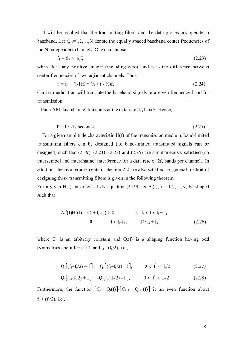
It will be recalled that the transmitting filters and the data processors operate in

baseband. Let fi, i=1,2,…,N denote the equally spaced baseband center frequencies of

the N independent channels. One can choose

f1 = (h + ½)fs (2.23)

where h is any positive integer (including zero), and fs is the difference between

center frequencies of two adjacent channels. Thus,

fi = f1 + (i-1)fs = (h + i - ½)fs (2.24)

Carrier modulation will translate the baseband signals to a given frequency band for

transmission.

Each AM data channel transmits at the data rate 2fs bauds. Hence,

T = 1 / 2fs seconds (2.25)

For a given amplitude characteristic H(f) of the transmission medium, band-limited

transmitting filters can be designed (i.e band-limited transmitted signals can be

designed) such that (2.19), (2.21), (2.22) and (2.25) are simultaneously satisfied (no

intersymbol and interchannel interference for a data rate of 2fs bauds per channel). In

addition, the five requirements in Section 2.2 are also satisfied. A general method of

designing these transmitting filters is given in the following theorem.

For a given H(f), in order satisfy equation (2.19), let Ai(f), i = 1,2,…,N, be shaped

such that

Ai2(f)H2(f) = Ci + Qi(f) > 0, fi - fs < f < fi + fs

= 0 f < fi-fs, f > fi + fs (2.26)

where Ci is an arbitrary constant and Qi(f) is a shaping function having odd

symmetries about fi + (fs/2) and fi - (fs/2), i.e.,

Qi[(fi+fs/2) + f′] = -Qi[(fi+fs/2) - f′], 0 < f′ < fs/2 (2.27)

Qi[(fi-fs/2) + f′] = -Qi[(fi-fs/2) - f′], 0 < f′ < fs/2 (2.28)

Furthermore, the function [Ci + Qi(f)]⋅[Ci+1 + Qi+1(f)] is an even function about

fi + (fs/2), i.e.,

18

[Ci + Qi(fi + fs/2+f′)]⋅[Ci+1 + Qi+1(fi + fs/2+f′)]

= [Ci + Qi(fi + fs/2-f′)]⋅[Ci+1 + Qi+1(fi + fs/2-f′)]

0 < f′ < fs/2 i = 1,2, … .N-1 (2.29)

By considering even symmetry of Cos 2πfkT and odd symmetry of Sin 2πfkT about

fi + (fs/2) for all k, from equation (2.21) and (2.22) let the phase characteristic

αi(f), i = 1,2, … N, be shaped such that

αi(f) - αi+1(f) = ± π/2 + γi(f), fi < f < fi + fs

i = 1,2, …, N-1, (2.30)

where γi(f) is an arbitrary phase function with odd symmetry about fi + (fs/2).

If Ai(f) and αi(f) are shaped as in (2.26) through (2.30) and f1 is set according to

(2.23), then (2.19), (2.21), (2.22) and (2.25) are simultaneously satisfied (no

intersymbol or interchannel interference for a data rate of 2fs bauds per channel).

Furthermore, the five requirements in section 2.2 are also satisfied.

2.2.2 Transmission filter characteristics:

Consider first the shaping of the amplitude characteristics Ai(f) of the transmitting

filters. Equations (2.26), (2.27) and (2.28) can be easily satisfied. Equation (2.29) can

be satisfied in many ways. For instance, a simple, practical way to satisfy (2.29) is

given below.

Under the simplifying condition that

(i) Ci should be the same for all i

(ii) Qi(f), i = 1,2, …, N, should be identically shaped, i.e.,

Qi+1(f) = Qi(f-fs), i = 1, 2, …, N-1, (2.31)

Equation (2.29) holds when Qi(f) is an even function about fi, i.e.,

Qi(fi + f′) = Qi(fi - f′), 0 < f′< fs. (2.32)

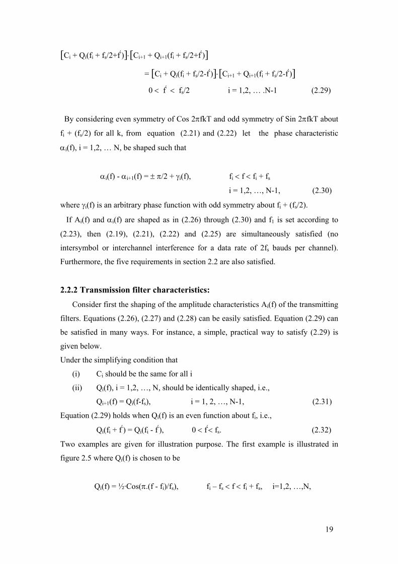
Two examples are given for illustration purpose. The first example is illustrated in

figure 2.5 where Qi(f) is chosen to be

Qi(f) = ½·Cos(π.(f - fi)/fs), fi – fs < f < fi + fs, i=1,2, …,N,

19

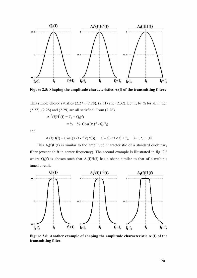
Figure 2.5: Shaping the amplitude characteristics Ai(f) of the transmitting filters

This simple choice satisfies (2.27), (2.28), (2.31) and (2.32). Let Ci be ½ for all i, then

(2.27), (2.28) and (2.29) are all satisfied. From (2.26)

Ai 2(f)H2(f) = Ci + Qi(f)

= ½ + ½⋅ Cos((π.(f - fi)/fs)

and

Ai(f)H(f) = Cos((π.(f - fi)/(2fs)), fi – fs < f < fi + fs, i=1,2, …,N.

This Ai(f)H(f) is similar to the amplitude characteristic of a standard duobinary

filter (except shift in center frequency). The second example is illustrated in fig. 2.6

where Qi(f) is chosen such that Ai(f)H(f) has a shape similar to that of a multiple

tuned circuit.

Figure 2.6: Another example of shaping the amplitude characteristic Ai(f) of the transmitting filter.

20

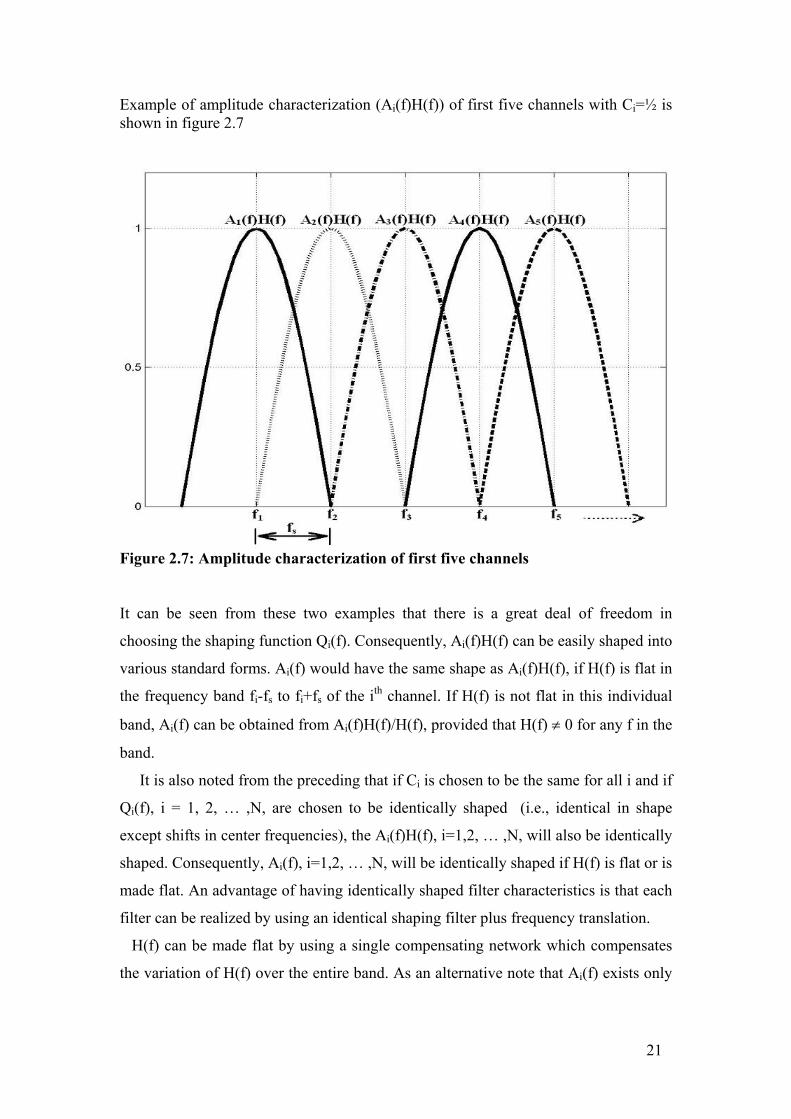
Example of amplitude characterization (Ai(f)H(f)) of first five channels with Ci=½ is shown in figure 2.7

Figure 2.7: Amplitude characterization of first five channels It can be seen from these two examples that there is a great deal of freedom in

choosing the shaping function Qi(f). Consequently, Ai(f)H(f) can be easily shaped into

various standard forms. Ai(f) would have the same shape as Ai(f)H(f), if H(f) is flat in

the frequency band fi-fs to fi+fs of the ith channel. If H(f) is not flat in this individual

band, Ai(f) can be obtained from Ai(f)H(f)/H(f), provided that H(f) ≠ 0 for any f in the

band.

It is also noted from the preceding that if Ci is chosen to be the same for all i and if

Qi(f), i = 1, 2, … ,N, are chosen to be identically shaped (i.e., identical in shape

except shifts in center frequencies), the Ai(f)H(f), i=1,2, … ,N, will also be identically

shaped. Consequently, Ai(f), i=1,2, … ,N, will be identically shaped if H(f) is flat or is

made flat. An advantage of having identically shaped filter characteristics is that each

filter can be realized by using an identical shaping filter plus frequency translation.

H(f) can be made flat by using a single compensating network which compensates

the variation of H(f) over the entire band. As an alternative note that Ai(f) exists only

21

from fi-fs to fi+fs. Hence, for the ith receiver, the integration limits of (2.19), (2.21) and

(2.22) can be changed to fi-fs and fi+fs. Therefore, the signal at the ith receiver only has

to satisfy the theorem in the limited frequency band fi-fs to fi+fs. This permits one to

design the transmitting filters for flat H(f) and then compensate the variation of H(f)

individually at the receivers, i.e., use an individual network at the ith receiver to

compensate only for the variation of H(f) in the limited frequency band fi-fs to fi+fs.

Finally, note that if the channels are narrow, each channel will usually be

approximately flat. In these cases, one may design the transmitting filters for flat H(f)

without using compensating networks. This design should lead to only small

distortion.

Consider next the shaping of the phase characteristics αi(f) of the transmitting

filters. It is only required that (2.30) be satisfied. However, if it is desired to have

identically shaped transmitting filter characteristics, one may consider a simple

method such as follows –

Under the simplifying condition that αi(f), i = 1,2, … ,N, be identically shaped, i.e.,

αi+1(f) = αi(f-fs) i = 1,2, … ,N-1 (2.33)

(2.30) holds when

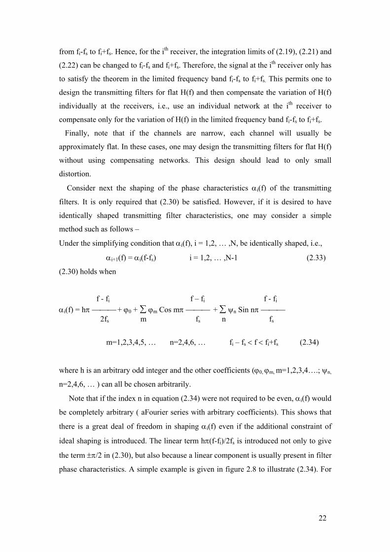
f - fi f – fi f - fi αi(f) = hπ + ϕ0 + ∑ ϕm Cos mπ + ∑ ψn Sin nπ 2fs m fs n fs

m=1,2,3,4,5, … n=2,4,6, … fi – fs < f < fi+fs (2.34)

where h is an arbitrary odd integer and the other coefficients (ϕ0, ϕm, m=1,2,3,4….; ψn,

n=2,4,6, … ) can all be chosen arbitrarily.

Note that if the index n in equation (2.34) were not required to be even, αi(f) would

be completely arbitrary ( aFourier series with arbitrary coefficients). This shows that

there is a great deal of freedom in shaping αi(f) even if the additional constraint of

ideal shaping is introduced. The linear term hπ(f-fi)/2fs is introduced not only to give

the term ±π/2 in (2.30), but also because a linear component is usually present in filter

phase characteristics. A simple example is given in figure 2.8 to illustrate (2.34). For

22

clarity, the arbitrary Fourier coefficients are all set to zero, except ψ2 = 0.3 and h is set

to -1.

Figure 2.8: Example of h = -1, ψ2 ≠ 0, all other coefficient zero.

As can be seen in the theorem, the requirement on αi(f) is independent of the

requirements on Ai(f). Hence, the amplitude and the phase characteristics of the

transmitting filters can be synthesized independently. This gives even more freedom

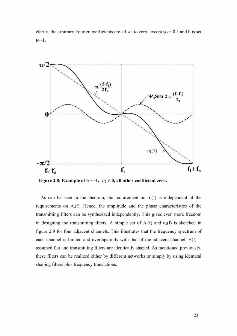
in designing the transmitting filters. A simple set of Ai(f) and αi(f) is sketched in

figure 2.9 for four adjacent channels. This illustrates that the frequency spectrum of

each channel is limited and overlaps only with that of the adjacent channel. H(f) is

assumed flat and transmitting filters are identically shaped. As mentioned previously,

these filters can be realized either by different networks or simply by using identical

shaping filters plus frequency translations.

23

Figure 2.9: Transmitting filter characteristics for orthogonal multiplexing

data transmission

Now consider the five requirements in Section 2.2. The first requirement is

satisfied since the transmitting filters designed are of standard forms. Perpendicular

cutoffs and linear phase characteristics are not required.

As for the second requirement, it can be seen from figure 2.9 that the overall

baseband bandwidth of N channels is (N+1)fs. Since data rate per channel is 2fs bauds,

the overall data rate of N channels is 2fsN bauds. Hence,

Overall data rate = [2N/(N+1)] . Overall baseband bandwidth

= [N/(N+1)] . Rmax ,

Where Rmax, which equals two times overall baseband bandwidth, is the Nyquist rate

for which unrealizable filters with perpendicular cutoffs and linear phases are

required. Thus, for moderate values of N, the overall data rate of the orthogonal

multiplexing data transmission system is close to the Nyquist rate, yet rectangular

filtering is not required. This satisfies second requirement.

24

Now consider the third requirement. As has been shown, the received pulses are

orthogonal if (2.19), (2.21) and (2.22) are simultaneously satisfied. Note that the

phase characteristic η(f) of the transmission medium does not enter into these

equations. Hence, the received signals will remain orthogonal for all η(f), and

adaptive correlation reception can be used no matter what the phase distortion is in the

transmission medium. Also note that so far as each receiver is concerned, the phase

characteristics of the networks in each receiver (including the bandpass filter at the

input of each receiver) can be considered as part of η(f), and hence has no effect on

the orthogonality of the received signals.

In the case of the fourth requirement, let

bki, k = 0, 1, 2, …; i = 1, 2, … ,N,

and

cki, k = 0, 1, 2, …; i = 1, 2, … ,N,

be two arbitrary distinct sets of m-ary signal digits or real numbers to be transmitted

by the N channels. The distance in signal space between the two sets of received

signals

∑ ∑ bki ui(t - kT)

i k and

∑ ∑ cki ui(t - kT)

i k is

∞

d = [ ∫ [∑ ∑ bki ui(t - kT) - ∑ ∑ ck

i ui(t - kT) ]2 dt ]½

-∞ i k i k

In an ideal case where transmitting the signals of each channel through an

independent medium eliminates interchannel and intersymbol interferences and

slowing down data rate such that the received signals in each channel do not overlap,

25

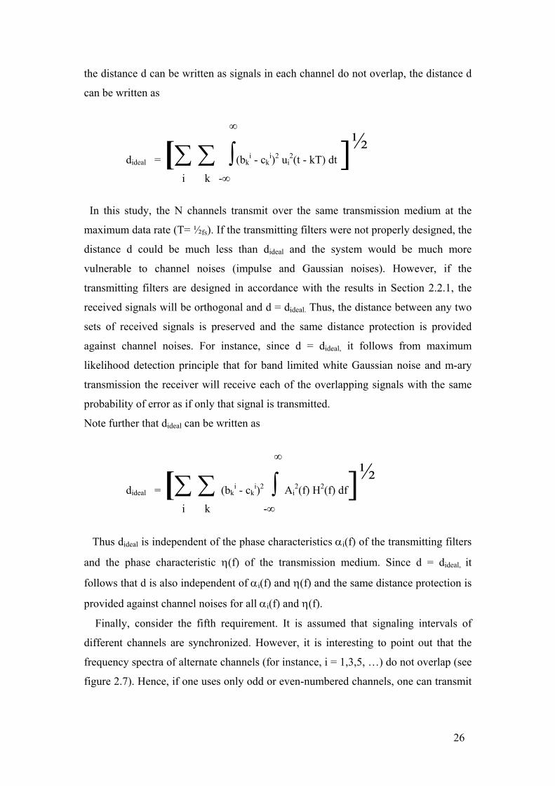
the distance d can be written as signals in each channel do not overlap, the distance d

can be written as

∞

dideal = [∑ ∑ ∫ (bki - ck

i)2 ui2(t - kT) dt ]½

i k -∞

In this study, the N channels transmit over the same transmission medium at the

maximum data rate (T= ½fs). If the transmitting filters were not properly designed, the

distance d could be much less than dideal and the system would be much more

vulnerable to channel noises (impulse and Gaussian noises). However, if the

transmitting filters are designed in accordance with the results in Section 2.2.1, the

received signals will be orthogonal and d = dideal. Thus, the distance between any two

sets of received signals is preserved and the same distance protection is provided

against channel noises. For instance, since d = dideal, it follows from maximum

likelihood detection principle that for band limited white Gaussian noise and m-ary

transmission the receiver will receive each of the overlapping signals with the same

probability of error as if only that signal is transmitted.

Note further that dideal can be written as

∞

dideal = [∑ ∑ (bki - ck

i)2 ∫ Ai2(f) H2(f) df]½

i k -∞

Thus dideal is independent of the phase characteristics αi(f) of the transmitting filters

and the phase characteristic η(f) of the transmission medium. Since d = dideal, it

follows that d is also independent of αi(f) and η(f) and the same distance protection is

provided against channel noises for all αi(f) and η(f).

Finally, consider the fifth requirement. It is assumed that signaling intervals of

different channels are synchronized. However, it is interesting to point out that the

frequency spectra of alternate channels (for instance, i = 1,3,5, …) do not overlap (see

figure 2.7). Hence, if one uses only odd or even-numbered channels, one can transmit

26

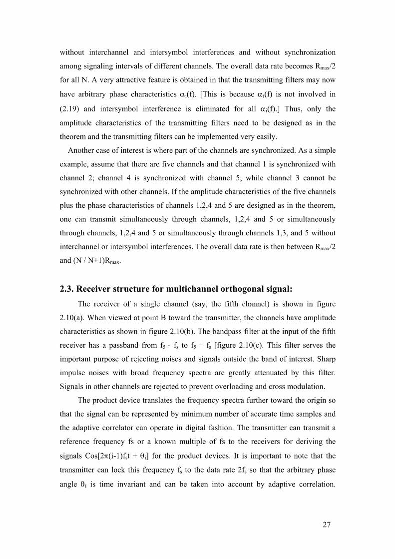
without interchannel and intersymbol interferences and without synchronization

among signaling intervals of different channels. The overall data rate becomes Rmax/2

for all N. A very attractive feature is obtained in that the transmitting filters may now

have arbitrary phase characteristics αi(f). [This is because αi(f) is not involved in

(2.19) and intersymbol interference is eliminated for all αi(f).] Thus, only the

amplitude characteristics of the transmitting filters need to be designed as in the

theorem and the transmitting filters can be implemented very easily.

Another case of interest is where part of the channels are synchronized. As a simple

example, assume that there are five channels and that channel 1 is synchronized with

channel 2; channel 4 is synchronized with channel 5; while channel 3 cannot be

synchronized with other channels. If the amplitude characteristics of the five channels

plus the phase characteristics of channels 1,2,4 and 5 are designed as in the theorem,

one can transmit simultaneously through channels, 1,2,4 and 5 or simultaneously

through channels, 1,2,4 and 5 or simultaneously through channels 1,3, and 5 without

interchannel or intersymbol interferences. The overall data rate is then between Rmax/2

and (N / N+1)Rmax.

2.3. Receiver structure for multichannel orthogonal signal: The receiver of a single channel (say, the fifth channel) is shown in figure

2.10(a). When viewed at point B toward the transmitter, the channels have amplitude

characteristics as shown in figure 2.10(b). The bandpass filter at the input of the fifth

receiver has a passband from f5 - fs to f5 + fs [figure 2.10(c). This filter serves the

important purpose of rejecting noises and signals outside the band of interest. Sharp

impulse noises with broad frequency spectra are greatly attenuated by this filter.

Signals in other channels are rejected to prevent overloading and cross modulation.

The product device translates the frequency spectra further toward the origin so

that the signal can be represented by minimum number of accurate time samples and

the adaptive correlator can operate in digital fashion. The transmitter can transmit a

reference frequency fs or a known multiple of fs to the receivers for deriving the

signals Cos[2π(i-1)fst + θi] for the product devices. It is important to note that the

transmitter can lock this frequency fs to the data rate 2fs so that the arbitrary phase

angle θi is time invariant and can be taken into account by adaptive correlation.

27

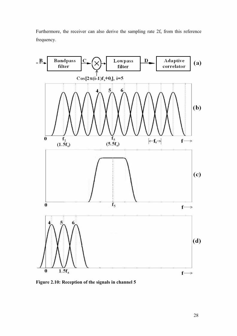
Furthermore, the receiver can also derive the sampling rate 2fs from this reference

frequency.

Figure 2.10: Reception of the signals in channel 5

28

When observed at point D, the channels have amplitude characteristics as shown

in figure 2.10(d). Note that the fifth channel now has a center frequency at 1.5fs

[satisfying (2.24)] and an undistorted amplitude characteristic; hence, the signals in

channel 5 remain orthogonal. The overlapping frequency spectra between channel 5

and channels 4 and 6 remain undistorted, and the phase differences α4(f) - α5(f) and

α5(f) - α6(f) are unchanged; therefore, the signals in channels 4 and 6 remain

orthogonal to those in channel 5. Other channels produce no interference since their

spectra do not overlap with that of channel 5.

Let b0u(t), b1u(t-T), b2u(t-2T), … be the signals in channel 5 at point D, where

b0, b1, b2, … are the information digits. These signals can be represented by vectors of

time samples as

b0u0, b1u1, b2u2, …

Since u(t), u(t – T), … differ only in time origin, it is only necessary to learn u0 for

correlation purposes. The received signal at point D can be written as

∑ bnun + v n where v represents the sum of the signals in other channels. Here due to orthogonality

uk′uj = λ k = j

= 0 k ≠ j

uk′v = 0.

Thus, the adaptive correlator can learn the vector u0 prior to data transmission and

then correlate the received signal with uk, k = 0,1,2, … to obtain the information digits

bk, k = 0,1,2, ….

29

Chapter 3.

OFDM: FFT Based Approach

For a large number of channels, the arrays of sinusoidal generators and coherent

demodulators required in parallel systems become unreasonably expensive and

complex [9]. However, it can be shown [10] that a multitone data signal is effectively

the Fourier transform of the original serial data train, and that the bank of coherent

demodulators is effectively an inverse Fourier transform generator. This point of view

suggests a completely digital modem built around a special-purpose computer

performing the fast Fourier transform (FFT). Fourier transform techniques, although

not necessarily the signal format described here. This innovation had a tradeoff in that

their system could not guarantee orthogonality between subcarriers over a dispersive

channel. In 1980, A Peled and A Ruiz solved the orthogonality problem with their

introduction of the cyclic prefix (CP) [11]. The cyclic prefix is a copy of the last part

of the OFDM symbol attached to the front of the transmitted symbol. When the CP

length is longer than the channel impulse response, the received signal is a cyclic

convolution of the transmitted signal and the channel impulse response. The cyclic

convolution results in the orthogonality of the subcarriers being maintained over a

dispersive channel.

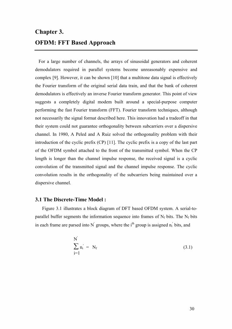
3.1 The Discrete-Time Model : Figure 3.1 illustrates a block diagram of DFT based OFDM system. A serial-to-

parallel buffer segments the information sequence into frames of Nf bits. The Nf bits

in each frame are parsed into N′ groups, where the ith group is assigned ni′ bits, and

N′

∑ ni′ = Nf (3.1)

i=1

30

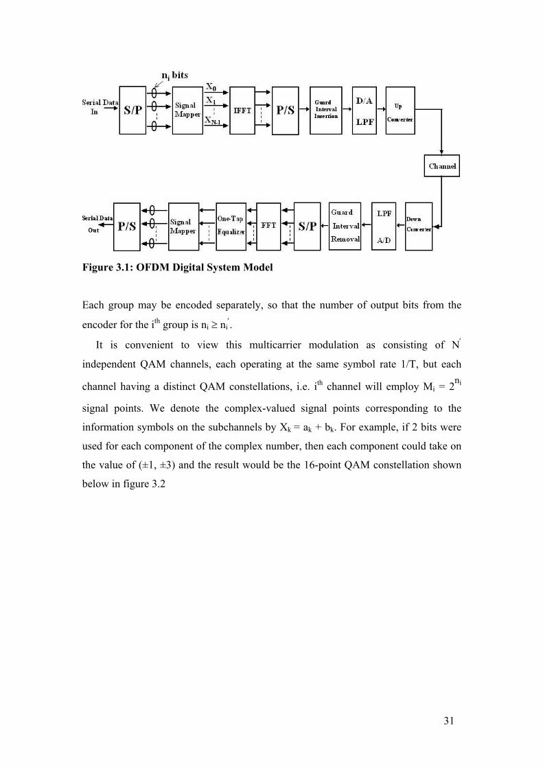
Figure 3.1: OFDM Digital System Model

Each group may be encoded separately, so that the number of output bits from the

encoder for the ith group is ni ≥ ni′.

It is convenient to view this multicarrier modulation as consisting of N′

independent QAM channels, each operating at the same symbol rate 1/T, but each

channel having a distinct QAM constellations, i.e. ith channel will employ Mi = 2ni

signal points. We denote the complex-valued signal points corresponding to the

information symbols on the subchannels by Xk = ak + bk. For example, if 2 bits were

used for each component of the complex number, then each component could take on

the value of (±1, ±3) and the result would be the 16-point QAM constellation shown

below in figure 3.2

31

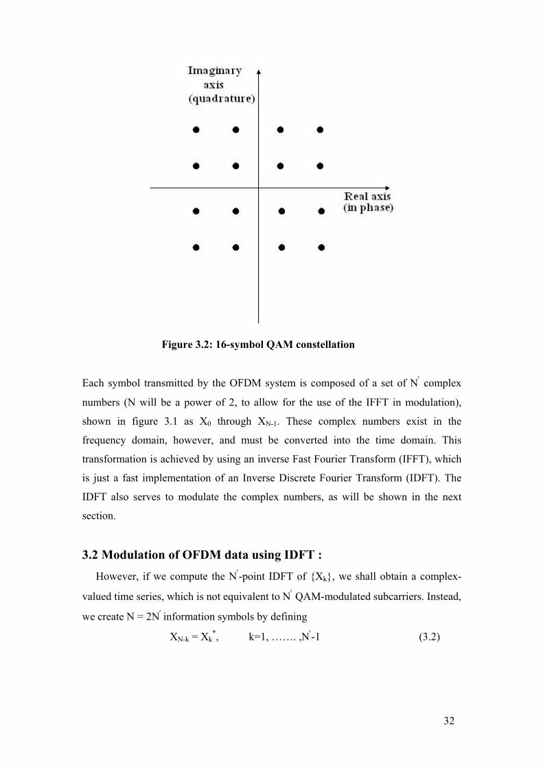
Figure 3.2: 16-symbol QAM constellation

Each symbol transmitted by the OFDM system is composed of a set of N′ complex

numbers (N will be a power of 2, to allow for the use of the IFFT in modulation),

shown in figure 3.1 as X0 through XN-1. These complex numbers exist in the

frequency domain, however, and must be converted into the time domain. This

transformation is achieved by using an inverse Fast Fourier Transform (IFFT), which

is just a fast implementation of an Inverse Discrete Fourier Transform (IDFT). The

IDFT also serves to modulate the complex numbers, as will be shown in the next

section.

3.2 Modulation of OFDM data using IDFT :

However, if we compute the N′-point IDFT of {Xk}, we shall obtain a complex-

valued time series, which is not equivalent to N′ QAM-modulated subcarriers. Instead,

we create N = 2N′ information symbols by defining

XN-k = Xk*, k=1, ……. ,N′-1 (3.2)

32

And X0 = Re{X0}, and XN′ = Im(X0). Thus, the symbol X0 is split into two parts, both

real. Then the N-point IDFT yields the real-valued sequence

1 N-1

xn = ∑ Xk eJ2πnk / N , n = 0,1,2,…N-1 (3.3) √N k=0

where 1/√N is simply a scale factor.

The sequence {xn, 0 ≤ n ≤ N-1} corresponds to the samples of the sum x(t) of N′

subcarrier signals, which is expressed as

1 N-1

x(t) = ∑ Xk eJ2πkt / T , 0 ≤ t ≤ T (3.4) √N k=0

where T is the symbol duration. We observe that the subcarrier frequencies are

fk = k/T, k=0,1,2….N′. Furthermore, the discrete-time sequence {xn} in equation (3.3)

represents the samples of x(t) taken at times t=nT/N where n = 0,1,2, …, N-1.

The resulting baseband signal is then converted back into serial data and undergoes

the addition of the cyclic prefix (which will be explained in the next section). In

practice, the signal samples {xn} are passed through a digital-to-analog (D/A)

converter at time intervals T/N. Next, the signal is passed through a low-pass filter to

remove any unwanted high-frequency noise, whose output, ideally, would be the

signal waveform x(t). The resulting signal closely approximates the frequency

division multiplexed signal.

The last step in the transmission process is to convert the signals from baseband to

bandpass by stepping up each subcarrier frequency in the up converter.

Because of the rectangular windowing of the above function (0 ≤ t ≤ T), the spectrum

of each subcarrier (at carrier frequency fk) is a Sinc function as shown in figure 3.3.

33

Figure 3.3: Spectra of OFDM subchannels

3.3 Orthogonality : From equation (3.3) it can be shown that in resultant equation of xn, each Xk is

multiplied by

1 φk(n) = eJ2πnk / N n = 0,1,2,…N-1, ∀ k ∈ [0, N-1] √N It can be very easily shown that the inner product –

<φm(n), φn(n)> = 1 m = n

= 0 m ≠ n (3.5)

where m,n are any integers ranging from 0 to N-1. Thus orthogonality is maintained

in the exponentials associated with every set of different subchannels. This definition

can also be loosely applied to the frequency domain as well: Orthogonality of OFDM

34

subcarriers is maintained so long as all subcarriers are sampled at their peaks, where a

null exists for the spectra of all other subcarriers. That is, at any subcarrier peak the

product of that particular subcarrier’s spectrum and any other subcarrier’s spectrum

will be equal to zero, causing inner product to yield zero and satisfy the criteria for

orthogonality.

3.4 The cyclic prefix : Orthogonality of OFDM subcarriers is critical since it prevents interchannel

interference. As such, OFDM is highly sensitive to frequency dispersion caused by

Doppler shifts [12]. If an OFDM receiver is mobile and moving towards the

transmitter, the Doppler shift can cause a corresponding shift in the OFDM spectrum.

This frequency shift causes a subcarrier to be sampled at a frequency other than the

one corresponding to its peak. As a result, orthogonality is lost and there is a

reduction in the signal amplitude as well as intercarrier interference. The solution for

this is the cyclic prefix.

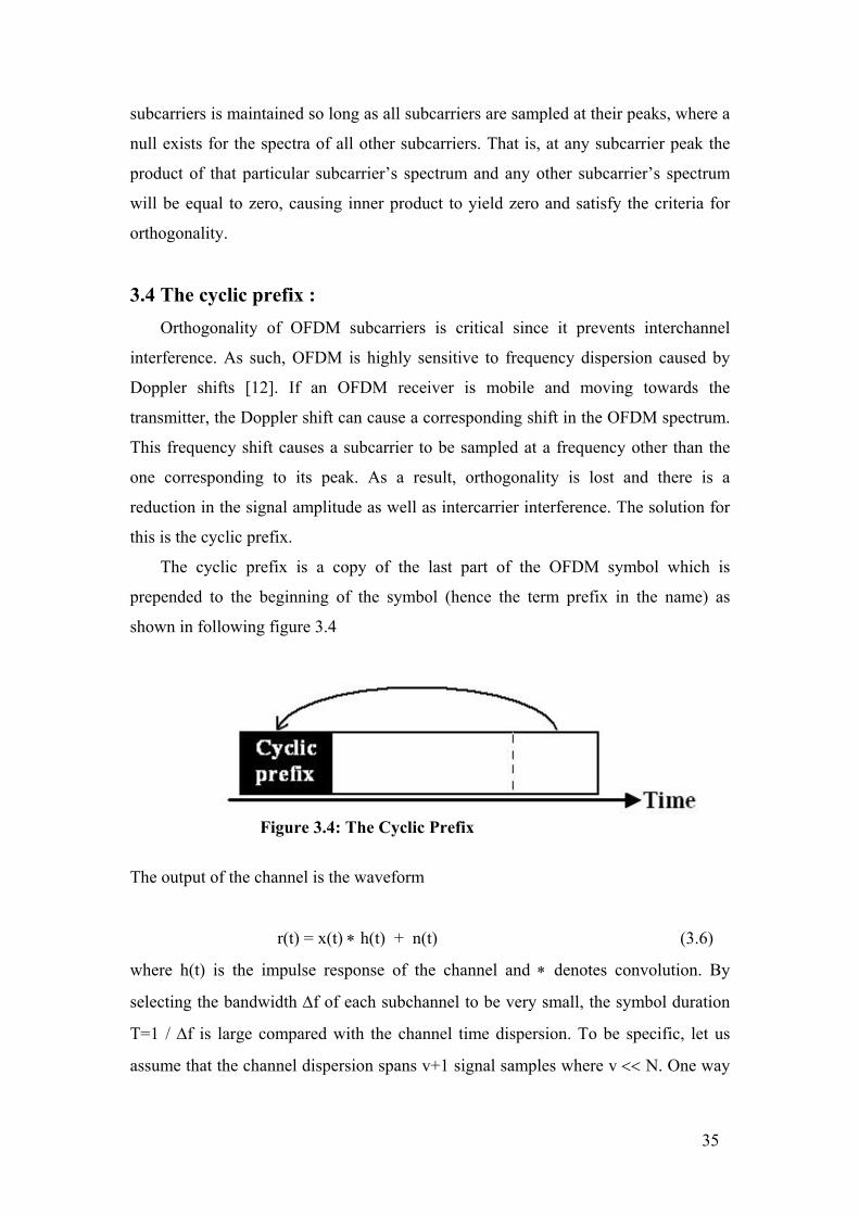
The cyclic prefix is a copy of the last part of the OFDM symbol which is

prepended to the beginning of the symbol (hence the term prefix in the name) as

shown in following figure 3.4

Figure 3.4: The Cyclic Prefix

The output of the channel is the waveform

r(t) = x(t) ∗ h(t) + n(t) (3.6)

where h(t) is the impulse response of the channel and ∗ denotes convolution. By

selecting the bandwidth ∆f of each subchannel to be very small, the symbol duration

T=1 / ∆f is large compared with the channel time dispersion. To be specific, let us

assume that the channel dispersion spans v+1 signal samples where v << N. One way

35

to avoid the effect of ISI is to insert a time guard band of duration vT/N between

transmission of successive blocks.

An alternative method that avoids ISI is to append a cyclic prefix to each block of

N signal samples {x0, x1, …, xN-1}. These new samples are appended to the beginning

of each block. Note that the addition of the cyclic prefix to the block of data increases

the length of the block to N+v samples, which may be indexed from n=-v, …, N-1,

where the first v samples constitute the prefix. Then, if {hn, 0 ≤ n ≤ v} denotes the

sampled channel impulse response, its convolution with {xn, -v ≤ n ≤ N-1} produces

{rn}, the received sequence. We are interested in the samples of {rn} for 0 ≤ n ≤ N-1,

from which we recover the transmitted sequence by using the N-point DFT for

demodulation. Thus the first v samples of {rn} are discarded.

Thus cyclic prefix serves two very important purposes. First, it acts as a guard space

between transmitted symbols. The length of the cyclic prefix is usually less than ¼ the

length of the symbol period, but is assumed to be longer than the RMS delay spread

of the channel. So when the cyclic prefix is removed in the receiver, the delay spread

contained within it is also removed. Thus, time dispersion and ISI are avoided.

Second, since the cyclic prefix is assumed longer than the channel impulse response,

r(t) appears to the channel as a periodic signal and the channel impulse response can

be cyclically convolved with the signal. Because of this cyclic convolution, the

orthogonality of the subcarriers is maintained [11] and ICI is avoided.

3.5 Demodulation using the DFT : From a frequency-domain viewpoint, when the channel impulse response is

{hn, 0 ≤ n ≤ v}, its frequency response at the subcarrier frequencies fk = k/N is

v Hk ≡ H(2πk / N) = ∑ hn e-J2πk / N (3.7)

n=0

Because of the cyclic prefix, successive blocks (frames) of the transmitted

information sequence do not interfere and, hence, the demodulated sequence may be

expressed as

Xk′ = HkXk + ηk, k = 0,1, …, N-1 (3.8)

36

Where {Xk′} is the output of the N-point DFT demodulator, and ηk is the additive

noise corrupting the signal. We note that by selecting N >> v, the rate loss due to the

cyclic prefix can be rendered negligible.

As shown in figure 3.1, the information is demodulated by computing the DFT of

the received signal after it has been passed through an analog-to-digital (A/D)

converter. As in the case of the modulator, the DFT computation at the demodulator is

performed efficiently by use of the FFT algorithm. It is simple matter to estimate and

compensate for the channel factors {Hk} prior to passing the data to the detector and

decoder. A training signal consisting of either a known modulated sequence on each

of the subcarriers or unmodulated subcarriers may be used to measure the {Hk} at the

receiver. If the channel parameters vary slowly with time, it is also possible to track

the time variations by using the decisions at the output of the detector or the decoder,

in a decision directed fashion. Thus, this kind of multicarrier system can be rendered

adaptive.

Other types of implementation besides the DFT are possible. For example, a

digital filter bank that basically performs the DFT may be substituted for the FFT-

based implementation when the number of subcarriers is small, e.g., N ≤ 32. For a

large number of subcarriers, e.g. N > 32, the FFT-based systems are computationally

more efficient.

This OFDM multicarrier QAM of the type described above has been

implemented for a variety of applications, including high-speed transmission over

telephone lines, such as digital subcarrier lines.

37

Chapter 4.

The Downsides of OFDM

OFDM systems have a number of drawbacks [13]

1. Cyclic Prefix Overhead-

A cyclic prefix at least as long as the channel response must be attached to each

OFDM symbol to prevent interference between symbols. The cyclic prefix represents

a significant overhead and the only way to improve efficiency (reduce the relative

overhead) is to increase the number of subcarriers.

2. Frequency Control-

OFDM relies on orthogonality between the overlapped sub-carriers achieved by

frequency control to within one percent of the subcarrier spacing. Frequency offset

errors mean that the subcarriers are no longer orthogonal, resulting in intercarrier

interference and severe degradation in performance.

For example, a total 3.5 MHz bandwidth shared between 512 sub-channels gives a

frequency spacing of 6.8 KHz between subcarriers, requiring frequency accuracy

better than 68 Hz. For this reason, OFDM systems are very sensitive to both

frequency offsets and phase noise, and require costly, high specification radio

components. The larger the number of subcarriers, the closer the frequency spacing,

and so frequency accuracy becomes more and more critical. In Broadband Wireless

Access (BWA) systems, vehicles moving through the beam induce sporadic Doppler

shifts, resulting in additional frequency offset.

3. Requirement for coded or adaptive OFDM -

A null in the frequency response of the channel results in one or more subcarriers

having a very low SNR, and these subcarriers will dominate the overall error rate. For

this reason, OFDM without either power/rate adaptation, or coding, gives worse

performance than single carrier (SC) modulation. The full potential of OFDM can

only be achieved if power and bit rate are optimal for each individual subcarrier for

each individual receiver. This is not possible for broadcast transmission on the

downlink.

38

Another way to protect individual sub-carriers from frequency nulls, is to use

error-control coding. Coded OFDM gives similar performance to equalized SC

transmission [14], at the expense of very low coding rates, typically in the range 0.5 to

0.75. As well as reducing system throughput, the error-control code also increases

receiver complexity, particularly for convolutional codes.

4. Latency and block based processing -

Fast Fourier Transform (FFT) processing for OFDM is performed on blocks. If

the number of of subcarriers is increased, the FFT block size is also increased. Block-

based processing imposes a minimum block size for each transmitted packet, resulting

in delays and loss of efficiency for very small data bursts. The latency of OFDM is

high because the smallest burst that can be sent is a full OFDM block. Contrary SC

transmission is very efficient, because the block length can be reduced to fit the data

payload.

5. Synchronization-

Synchronization for OFDM transmission is more difficult, and typically requires

reception of several OFDM symbols, each having a number of subcarriers dedicated

for pilot tones. This is feasible for broadcast OFDM (such as HDTV), where the

receiver has plenty of time to acquire synchronization. However, for short burst,

point-to-multipoint transmission (especially on the uplink), there is little time to

acquire synchronization, and so complicated synchronization schemes are

necessary[15].

6. Peak-to-average power ratio (PAR) -

A major problem with OFDM is the relatively high PAR that is inherent in the

transmitted signal. In general, large signal peaks occur in the transmitted signal when

the signals in many of the various subchannels add constructively in phase. Such large

signal peaks may result in clipping of the signal voltage in a D/A converter when

multicarrier signal is synthesized digitally, and/or it may saturate the power amplifier

and, thus, cause intermodulation distortion in the transmitted signal.

39

Various methods have been devised to reduce the PAR in multicarrier systems.

One of the simplest methods is to insert different phase shifts in each of the

subcarriers. These phase shifts can be selected pseudorandomly, or by means of some

algorithm, to reduce the PAR. For example, we may have a small set of N stored

pseudorandomly selected phase shifts which can be used when the PAR in the

modulated subcarriers is large. The information on which set of pseudorandom phase

shifts is used in any signal interval can be transmitted to the receiver on one of the N

subcarriers. Alternatively, a single set of pseudorandom phase shifts may be

employed, where this set is found via computer simulation to reduce the PAR to an

acceptable level over the ensemble of possible transmitted data symbols on the N

subcarriers.

It is possible to achieve a small reduction in PAR using coding to avoid data

sequences with high peaks, although this reduces the useful data rate.

40

Chapter 5.

Future Directions

Unending appetite to achieve capacity, high data rate, minimum bit error rate

(BER), spectral efficiency and minimum power requirements are the main driving

forces behind future research efforts in OFDM. Various approaches to cope up with

the drawbacks given in previous chapter produces infinite possibilities for future

research. Few of them are given here-

• Channel estimation with diversity techniques and/or coding to compensate the

effect(s) of channel with delay/Doppler shifts and try to achieve optimum

values of capacity, BER etc.

• Appropriate combination of waveform shaping and frame overlap in time

limited OFDM without destroying orthogonality.

• Dynamic selection of phase shifts, data sequences and signal clipping or either

of the combination of those to reduce PAR

• Design of channel estimator with time/frequency correlations with adaptation.

• Adaptive subcarrier, bit, and power allocation to each subband to achieve

optimum values of capacity, BER, minimum power requirement etc.

• Any other combined approaches like OFDM-CDMA, OFDM-SDMA.

• Blind estimation techniques for symbol timing and carrier frequency offset.

• OFDM application specific DSP architectures.

And last but not least, efforts to make it user-centered technology for improvement of

quality of life of the individual.

41

References

1) R W Chang, "Synthesis of bandlimited orthogonal signals for multichannel data

transmission", Bell Systems Technical Journal, 45: pp.1775-1796, Dec. 1966

2) S BWeinstein and P.M.Ebert, "Data Transmission by Frequency--Division

Multiplexing Using the Discrete Fourier Transform", IEEE Tans. Commun. Technol.,

Vol. COM--19, No.5, pp.628--634, Oct. 1971.

3) B Hirosaki, "An Orthogonal--Multiplexed QAM System Using the Discrete Fourier

Transform", IEEE Tans. Commun. Technol., Vol. COM--29, No.7, pp.982- -989, July

1981.

4) L J Cimini,Jr., "Analysis and Simulation of a Digital Mobile Channel Using

Orthogonal Frequency Division Multiplexing", IEEE Tans. Commun., Vol. COM--33,

No.7, pp.665--675, July 1985.

5) M Alard and R Lassalle, "Principles of Modulation and Channel Coding for Digital

Broadcasting for Mobile Receivers", EBU Technical Review, No. 224, pp.168--190,

Aug. 1987.

6) B Le Floch, R Halbert--Lassalle and D.Castelain, "Digital Sound Broadcasting to

Mobile Receivers", IEEE Trans. Consumer Electronics., Vol. 73, No.4, pp.30--34,

Aug. 1989.

7) J A C Bingham, "Multicarrier Modulation for Data Transmission : An Idea Whose

Time Has Come", IEEE Commun. Mag., Vol. 28, No. 5, pp.5--14, May 1990.

8) H F Harmuth, "On the Transmission of Information by Orthogonal Time

Functions", AIEE Trans., pt. I (Communication and Electronics), pp.248--255, July

1960

42

9) S B Weinstein and P. M. Ebert, "Data Transmission by Frequency-Division

Multiplexing using the Discrete Fourier Transform", IEEE Trans. On Comm. Tech,

Vol. COM--19, No-5, pp.628--634, Oct. 1971

10) J Salz and S B Weinstein, "Fourier Transform Communication System", presented

at the Ass. Computer Machinery Conf. Computers and Communication, Pine

Mauntain, Ga., Oct. 1969

11) A Peled and A Ruiz, "Frequency Domain ata Transmission using reduced

computational complexity algorithms", Proc. IEEE Conf. Acoustic and Signal

Processing, 00.964--967, 1980

12) P A Bello, "Characterization of randomly time-variant linear channels", IEEE

Trans. on circuits and systems, vol. CS-11, no.4, pp.360--393, Dec. 1963

13) A Benyamin-Seeyar, "PHY Layer System Proposal for Sub-11 GHz BWA", IEEE

802.16 Task Group 3 submission, January 2001

14) A Gusmao, R Dinis, J Conceicao, N Esteves, "Comparison of tewo modulation

choices for broadband wireless communications", IEEE Vehicular Technology Conf.,

Tokyo, Japan, Vol.2, pp.1300-1305, Yr. 2000

15) B Y Prasetyo, F Said, A H Aghvami, "Fast burst synchronization technique for

OFDM-WLAN systems", IEE Proceedings - Communications, Vol.147, No.5,

pp.292--298, October 2000

43