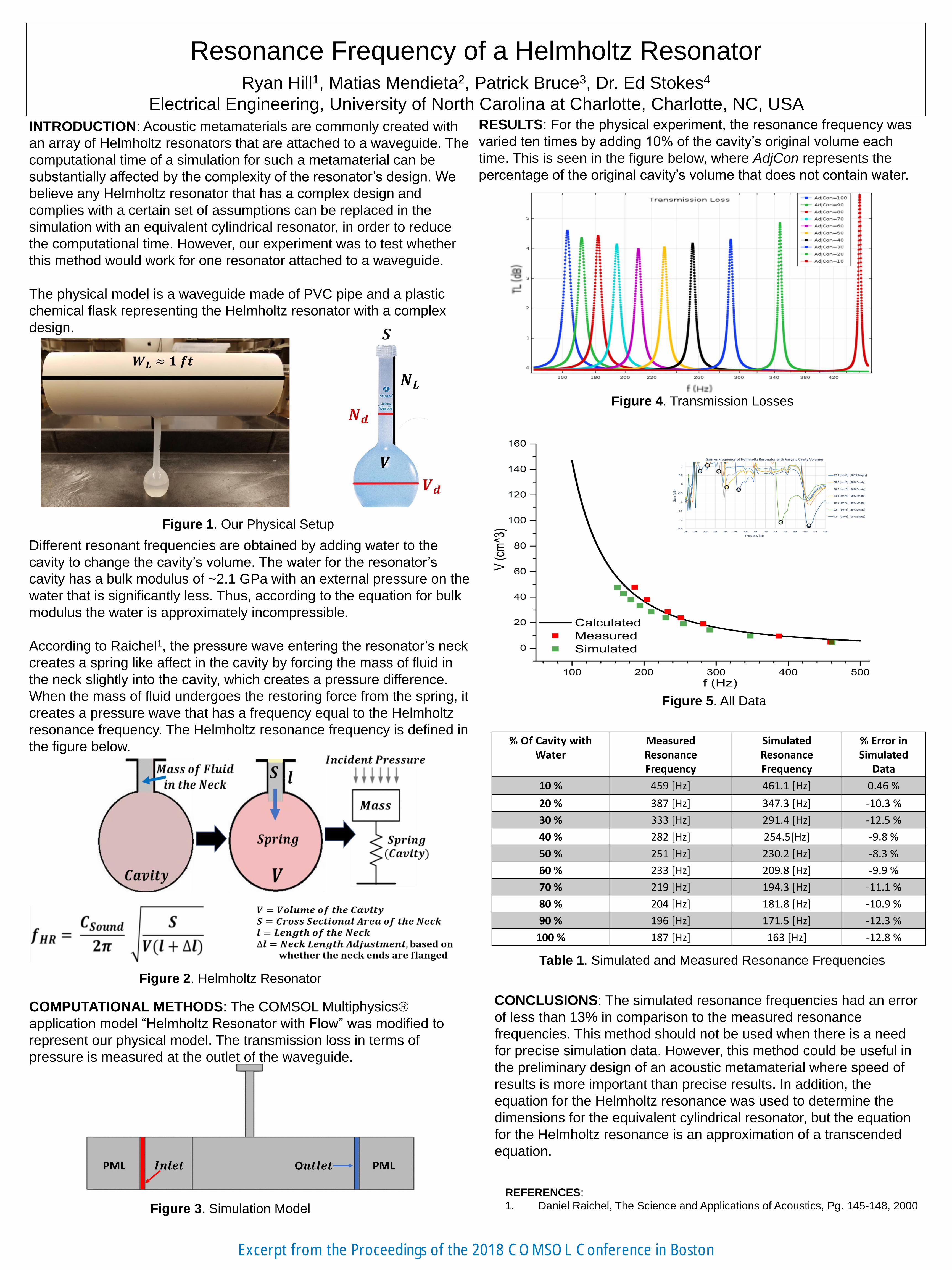
Resonance Frequency of a Helmholtz Resonator
1
INTRODUCTION: Acoustic metamaterials are commonly created with an array of Helmholtz resonators that are attached to a waveguide. The computational time of a simulation for such a metamaterial can be substantially affected by the complexity of the resonator’s design. We believe any Helmholtz resonator that has a complex design and complies with a certain set of assumptions can be replaced in the simulation with an equivalent cylindrical resonator, in order to reduce the computational time. However, our experiment was to test whether this method would work for one resonator attached to a waveguide. The physical model is a waveguide made of PVC pipe and a plastic chemical flask representing the Helmholtz resonator with a complex design. Different resonant frequencies are obtained by adding water to the cavity to change the cavity’s volume. The water for the resonator’s cavity has a bulk modulus of ~2.1 GPa with an external pressure on the water that is significantly less. Thus, according to the equation for bulk modulus the water is approximately incompressible. According to Raichel 1 , the pressure wave entering the resonator’s neck creates a spring like affect in the cavity by forcing the mass of fluid in the neck slightly into the cavity, which creates a pressure difference. When the mass of fluid undergoes the restoring force from the spring, it creates a pressure wave that has a frequency equal to the Helmholtz resonance frequency. The Helmholtz resonance frequency is defined in the figure below. COMPUTATIONAL METHODS: The COMSOL Multiphysics® application model “Helmholtz Resonator with Flow” was modified to represent our physical model. The transmission loss in terms of pressure is measured at the outlet of the waveguide. RESULTS: For the physical experiment, the resonance frequency was varied ten times by adding 10% of the cavity’s original volume each time. This is seen in the figure below, where AdjCon represents the percentage of the original cavity’s volume that does not contain water. CONCLUSIONS: The simulated resonance frequencies had an error of less than 13% in comparison to the measured resonance frequencies. This method should not be used when there is a need for precise simulation data. However, this method could be useful in the preliminary design of an acoustic metamaterial where speed of results is more important than precise results. In addition, the equation for the Helmholtz resonance was used to determine the dimensions for the equivalent cylindrical resonator, but the equation for the Helmholtz resonance is an approximation of a transcended equation. REFERENCES: 1. Daniel Raichel, The Science and Applications of Acoustics, Pg. 145-148, 2000 Table 1. Simulated and Measured Resonance Frequencies Figure 5. All Data Resonance Frequency of a Helmholtz Resonator Ryan Hill 1 , Matias Mendieta 2 , Patrick Bruce 3 , Dr. Ed Stokes 4 Electrical Engineering, University of North Carolina at Charlotte, Charlotte, NC, USA Figure 1. Our Physical Setup Figure 3. Simulation Model Figure 4. Transmission Losses % Of Cavity with Water Measured Resonance Frequency Simulated Resonance Frequency % Error in Simulated Data 10 % 459 [Hz] 461.1 [Hz] 0.46 % 20 % 387 [Hz] 347.3 [Hz] -10.3 % 30 % 333 [Hz] 291.4 [Hz] -12.5 % 40 % 282 [Hz] 254.5[Hz] -9.8 % 50 % 251 [Hz] 230.2 [Hz] -8.3 % 60 % 233 [Hz] 209.8 [Hz] -9.9 % 70 % 219 [Hz] 194.3 [Hz] -11.1 % 80 % 204 [Hz] 181.8 [Hz] -10.9 % 90 % 196 [Hz] 171.5 [Hz] -12.3 % 100 % 187 [Hz] 163 [Hz] -12.8 % Figure 2. Helmholtz Resonator Excerpt from the Proceedings of the 2018 COMSOL Conference in Boston
Transcript of Resonance Frequency of a Helmholtz Resonator
INTRODUCTION: Acoustic metamaterials are commonly created with
an array of Helmholtz resonators that are attached to a waveguide. The
computational time of a simulation for such a metamaterial can be
substantially affected by the complexity of the resonator’s design. We
believe any Helmholtz resonator that has a complex design and
complies with a certain set of assumptions can be replaced in the
simulation with an equivalent cylindrical resonator, in order to reduce
the computational time. However, our experiment was to test whether
this method would work for one resonator attached to a waveguide.
The physical model is a waveguide made of PVC pipe and a plastic
chemical flask representing the Helmholtz resonator with a complex
design.
Different resonant frequencies are obtained by adding water to the
cavity to change the cavity’s volume. The water for the resonator’s
cavity has a bulk modulus of ~2.1 GPa with an external pressure on the
water that is significantly less. Thus, according to the equation for bulk
modulus the water is approximately incompressible.
According to Raichel1, the pressure wave entering the resonator’s neck
creates a spring like affect in the cavity by forcing the mass of fluid in
the neck slightly into the cavity, which creates a pressure difference.
When the mass of fluid undergoes the restoring force from the spring, it
creates a pressure wave that has a frequency equal to the Helmholtz
resonance frequency. The Helmholtz resonance frequency is defined in
the figure below.
COMPUTATIONAL METHODS: The COMSOL Multiphysics®
application model “Helmholtz Resonator with Flow” was modified to
represent our physical model. The transmission loss in terms of
pressure is measured at the outlet of the waveguide.
RESULTS: For the physical experiment, the resonance frequency was
varied ten times by adding 10% of the cavity’s original volume each
time. This is seen in the figure below, where AdjCon represents the
percentage of the original cavity’s volume that does not contain water.
CONCLUSIONS: The simulated resonance frequencies had an error
of less than 13% in comparison to the measured resonance
frequencies. This method should not be used when there is a need
for precise simulation data. However, this method could be useful in
the preliminary design of an acoustic metamaterial where speed of
results is more important than precise results. In addition, the
equation for the Helmholtz resonance was used to determine the
dimensions for the equivalent cylindrical resonator, but the equation
for the Helmholtz resonance is an approximation of a transcended
equation.
REFERENCES:
1. Daniel Raichel, The Science and Applications of Acoustics, Pg. 145-148, 2000
Table 1. Simulated and Measured Resonance Frequencies
Figure 5. All Data
Resonance Frequency of a Helmholtz Resonator Ryan Hill1, Matias Mendieta2, Patrick Bruce3, Dr. Ed Stokes4
Electrical Engineering, University of North Carolina at Charlotte, Charlotte, NC, USA
Figure 1. Our Physical Setup
Figure 3. Simulation Model
Figure 4. Transmission Losses
% Of Cavity with Water
Measured Resonance Frequency
Simulated ResonanceFrequency
% Error inSimulated
Data
10 % 459 [Hz] 461.1 [Hz] 0.46 %
20 % 387 [Hz] 347.3 [Hz] -10.3 %
30 % 333 [Hz] 291.4 [Hz] -12.5 %
40 % 282 [Hz] 254.5[Hz] -9.8 %
50 % 251 [Hz] 230.2 [Hz] -8.3 %
60 % 233 [Hz] 209.8 [Hz] -9.9 %
70 % 219 [Hz] 194.3 [Hz] -11.1 %
80 % 204 [Hz] 181.8 [Hz] -10.9 %
90 % 196 [Hz] 171.5 [Hz] -12.3 %
100 % 187 [Hz] 163 [Hz] -12.8 %
Figure 2. Helmholtz Resonator
Excerpt from the Proceedings of the 2018 COMSOL Conference in Boston