1

Reservoir characterization using Monte Carlo simulation and Stochastic

analyses. Case studies: Off-shore Nile Delta and Ras Fanar oil field, Egypt

By

Aref Lashin1, 5

, Nassir Al Arifi 2

, Gamal Mousa 3

and Mohamed Abd El-Aal 4

1 Geology Department, Faculty of Science, Benha University, Egypt.

2 Geophysics Department, Faculty of Science, King Saud University, Riyadh, Saudi Arabia.

3 Mathematics Department, Faculty of Science, Benha University, Egypt.

4 Geology Department, Faculty of Education, Ain Shams University, Egypt.

5 AL-Qeeyah Community College, King Saud University, Saudi Arabia.

ABSTRACT

In this study, Monte Carlo simulation and stochastic modelling analyses, in combination with geological-

based concepts, are used to characterize the petrophysical parameters of the hydrocarbon-bearing reservoirs

by applying on two case studies in the off-shore Nile Delta and Ras Fanar oil field-Gulf of Suez, Egypt. The

stochastic input is supplied in the form of probability density functions, correlation, and variance-covariance

coefficients as determined from actual well logging data. The multivariate statistical analyses are used to

produce correlated multivariate stochastic variables. Two types of constraints (hard constraints and

simulation constraints) are used to guide and control the simulation procedure. Monte Carlo simulation

algorithm is then performed by running numerous iterations in front of each depth increment using the

correlated multivariate variables. A self-written visual basic programme is used to enhance the necessary

algorithms.

The model is applied in the off-shore Nile Delta, to improve the estimation of the petrophysical parameters

of the gas-bearing reservoirs. The available logging data are simulated to reduce the uncertainty in the final

interpretations which may arise from the statistics of counting and the transforms which are usually

associated with the recording of certain logs. Different Monte Carlo-based distributions are used to derive

the different parameters necessary for reservoir evaluation especially those of shale. The model is used also

to predict the petrophysical parameters of new exploratory wells providing that a satisfactory

topological/geological neighbourhood hard constraint is well developed in the area. In some fields of Gulf of

Suez (Ras Fanar field), the sonic log exhibits unique phenomenon (cycle skipping) due to the characteristic

acoustic properties of the Nullipore carbonate reservoir. The simulation algorithm is used to overcome this

problem using correlated multivariate variables of other related wells with good sonic records.

The simulated petrophysical parameters are found more realistic and representative for the studied reservoirs

in the off-shore Nile Delta and Gulf of Suez than those estimated using conventional logging analyses. It is

recommended to use this model in similar areas where the logging information is scarce or of bad quality

and also in new areas to secure optimum use of the available data. It can be further used as a predictive tool

for predicating the missed sections of old logs as well as the petrophysical parameters of the new exploratory

wells.

1. INTRODUCTION

Computer simulation using Monte Carlo methods provides a powerful tool for the analysis of the parameters

used in the volumetric studies, which is not possible using the traditional analytical approaches. The origin

of the modern Monte Carlo methods stems from work on the atomic bomb during the Second World War

when they were mainly used for numerical simulation of the neutron diffusion in fissile material, which is a

probabilistic problem. Later on, it was realized that Monte Carlo methods could also be used for

deterministic problems (Sambridge and Mosegaard, 2002).

Monte Carlo is a random sampling method and requires a large sampling number N for accurate estimation.

The algorithm relates and controls the uncertainty distributions of the individual parameters by a random

number function (between 0 and 1) which performs numerous random iterations for each distribution. So,

Monte Carlo simulation is used to solve certain stochastic (involving a random variable) problems where the

passage of time plays no substantive role. Nowadays, it is widely used to solve certain statistical problems

2

that are not analytically tractable. In geo-scientific applications, the method is used in many aspects such as

reserve estimation and for prospect evaluation (de Groot et al. 1996).

Many authors dealt with applying the geostatistical stochastic modelling and simulation techniques in

solving certain geological and petrophysical problems, of them the following are the most important; Bartlett

(1966); Rubinstein (1981); Haldorsen and Chang (1986); Isaaks and Srivastava (1989); Strauss and Sadler

(1989); Alabert and Massonnat (1990); Haldorsen and Damsleth (1990); Fogg et al. (1991); Law and Kelton

(1991); Bortoli, et al. (1993); de Groot et al. (1993 and 1996); Molz and Boman (1993), Deutsch (2002),

Pyrcz and Deutsch (2003); Pyrcz et al. (2005), ....etc.

2. MONTE CARLO SIMULATION AND RESERVOIR PARAMETERS

In conventional logging analyses, there are many difficulties concerning accurate estimation of the

petrophysical properties of the reservoir of interest. In many cases, the anticipated outcomes depend on

several input variables whose values may not be known exactly. Although, majority of logging data have to

be corrected before going in the interpretations, still some uncertainties in the final calculations may arise.

This can be argued in many cases to the methods by which some logs, especially the old ones, are recorded

and finally presented. The mathematical procedure used in counting and presenting the gamma ray log and

neutron porosity (far/near ratio) and the average method followed in calculating the interval transit time in

case of the compensated sonic log, are two examples of the expected uncertainties which could further

influence the final interpretations.

Another common problem, which if not treated carefully, may cause cumulative error in the calculations, is

the choice of some important parameters like; the shale and matrix ones. As the complexity of the system to

be interpreted increases, the conventional quantitative techniques used for reservoir analysis become more

and more unsuitable and uncertain. To deal with these problems, the actual well logging data can be

analyzed by a stochastic simulation method, such as Monte Carlo simulation to improve the estimation of

the properties of the reservoir of interest. The inputs are probability distributions, and the output of such

stochastic methods is also given in terms of distributions.

2.1 Uncertainty in Logging Data

As mentioned earlier, there are many reasons for the uncertainty in logging measurements. Most of the

expected errors are argued to the statistical methods which are followed while counting and converting

certain logging data from form to another. The following are some examples of these errors:

2.1.1 Error Propagation in the Statistics of GR Counting (CPS to API)

The natural gamma ray can be run in both open and cased holes, either empty or fluid-filled. This log may

be recorded in API units or counts per second, CPS. The nature of gamma ray emission is statistical and

must be averaged over time (Hearst and Nelson, 1985). The detector stability and the length of time required

to obtain a stable count rate depend upon the radioactivity of the target and efficiency of the detector. The

primary calibration standard of gamma ray tools is the API units. So, when measured in CPS units, the

gamma ray logs must be calibrated and converted to the API units.

Different statistical and probability distribution functions are used to model and calibrate the measured CPS

radioactive count rate in a given time window (t). The most important parameter which affects the

measurement is the count rate error. Using the rules of propagation of error, the count rate error can be

estimated as follows:

X Xσ = ………………………….….…… (1)

n X

t trσ = = ……………………………… (2)

2

200 *G

r

σσ

∆=

∆…………………...…………… (3)

API*Av

2

Xσ σσ = ………………….……........ (4)

3

where:

X is the number of counts per time window (t),

σX is the standard deviation,

σr is the count rate error,

t is the time windows (t),

σG is the calibration gain standard deviation,

σAv is the count rate error standard deviation.

Taking the count rate error in consideration, the raw gamma ray count rate in CPS can be converted and

calibrated to API units as follows:

( ) ( )r

API CPS200

GR = GR∆

…………………. (5)

GR fin (API) = GR (API) - σ Av …………. (6)

where:

GR (CPS) is the gamma ray in count per second,

GR (API) is the gamma ray in API units,

∆r is the count rate difference.

The previous statistical calibration is so complicated and in many cases leads to an expected effective error

in the raw values of the converted API gamma ray units. So all conventional well log analyses which make

use of gamma ray log will have some uncertainties and cause some errors in the final results, the effect

which could be eliminated if a suitable Monte Carlo distribution is used instead. It is worth to mention here,

that some environmental corrections of gamma ray log such as correction of gamma ray log for bore hole

condition and mud barite (GR-1 and GR-2 charts, Schlumberger Charts 1991) are based mainly on the

Monte Carlo simulation technique.

2.1.2 NPHI Porosity Estimation Form Dual Neutron (Ratio-to-Porosity Transform)

Porosity is one of the most important petrophysical properties, which must be carefully determined for good

evaluation and assessment of the reservoir of interest. Many logging tools are used for accurate porosity

estimation, among them is the dual neutron tool which is considered one of the most recent and important

tools. It employs a chemical source of neutrons and two thermal neutron detectors. The actual measurement

consists of the calibrated ratio of the far-detector to near-detector count rates (Mod-8 ratio to porosity

transform).

The far/near count ratio is related to the hydrogen content of the formation. When hydrogen is associated

with liquid-filled pore space, this ratio can be used to determine the classic NPHI porosity. The following is

the ratio-to-porosity transform which is used for fraction porosity estimation:

CPS

CPS

Far detector ( ) Ratio

Near detector ( )= …………… (7)

Having the porosity ratio, the environmentally uncorrected apparent limestone porosity can be estimated

using the special user function for the dual neutron probe as follows:

TMP3 = (TMP2)2 ………………………… (8)

TMP4 = (TMP2)3……………...…..….…… (9)

TMP5 = (0.1080258/ TMP4) - (0.25482/ TMP3) + (4.779079/ TMP2) - 9.517288 …... (10)

TMP6 = (0.1149102/ TMP4) - (0.25482/ TMP3) + (4.85726/ TMP2) - 8.734154 …… (11)

4

TMP7 = (TMP5 - TMP6) …...……………… (12)

TMP8 = TMP6 – (TMP7 * B.S) ..…………… (13)

NPHI = (TMP7 * TMP1) + TMP8 ………… (14)

where:

NPHI is the apparent limestone porosity,

TMP1 is the caliper log readings (mm),

TMP2 is the far/near ratio (CPS),

TMP7 and TMP8 are the slope and intercept of the calibrated porosities at borehole diameters of 214

mm and 150 mm, respectively.

The above mentioned statistical technique has the advantage of effectively compensating for the variations

in borehole and formation salinity from one hand and minimizing the effects of changes in borehole size

(caliper corrected) from the other hand. But still some difficulties and exaggerated errors in the final

estimated apparent porosity due to the normal regression analysis used for solving the equations.

2.2 Simulation Algorithm and Model Structure

Monte Carlo simulation can be used for a variety of different petrophysical problems, which are not so easy

to be treated by the traditional logging analyses. The procedure of Monte Carlo simulation depends on

numerous probabilities for certain samples to approximate the solution of any mathematical or physical

problem in a statistical way. The successful simulation model must be realistic representative of the

subsurface geological feature (reservoir) to be studied. So the input of the simulation algorithm is a

combination of stochastic correlated parameters and geological-based information controlled by certain

constraints.

To deal with the uncertainty, some rules are used in the reservoir simulation, the first are the petrophysical-

related ones which governorate the whole simulation framework, while the others are stochastic realizations

which can be re-evaluated and redrawn, until satisfactory result is achieved. The stochastic inputs are

supplied in the form of probability density functions (pdf’s) variance-covariance and correlation coefficients

matrices as determined from actual well logging data. A self designed visual-based programme was

constructed to estimate the different parameters necessary for running the simulation procedure. In addition

the Z-Rand software was used to create the random functions and finally the free DOE software is used for

conducting the necessary Monte Carlo simulation modules.

3. CONSTRAINTS

Before going on the simulation model, we have to define some constraints, which will guide and control the

simulation procedure. There are two types of constraints, hard constraints and simulation constraints. The

hard constraints, as used in this study, include number of probability density functions (pdf’s) for the

different studied zones, in addition to rules which keep the main petrophysical characteristics of different

zones (ρb - φN log responses in front of gas zones) and finally certain topo-geological relationship between

simulated wells in the area. At any stage of the simulation the stochastic variables are evaluated against the

hard constraints. If any hard constraint is not satisfied, then the variables are redrawn again and so on.

The simulation constraints, on the other hand, include petrophysical-related rules such as; shale and matrix

parameters, lithology type, and the number of different zones (entities) used in the study and their relative

thicknesses.

3.1 Correlated Stochastic Variables

In this study multiple geostatistical techniques are utilized to generate correlated distributions of the

reservoir rock parameters. Most of the utilized techniques are previously applied and taken from the work of

de Groot et al. 1996. To simplify the procedure, suppose that we have three correlated logging parameters or

variables (X1, X2 and X3), that satisfy the relation:

5

1 2 2E X X x = is linear in x2 ….… .(15)

1 3 3E X X x = is linear in x3 ……….… .(16)

Then it will be possible to get correlated stochastic variables of the logging data by constructing two types of

matrices (correlation and variance-covariance). By definition, the forms of these two matrices can be written

as follows:

Correlation Matrix Variance-Covariance Matrix

11 12 13

21 22 23

31 32 33

ρ ρ ρ

ρ ρ ρ

ρ ρ ρ

… (17)… and … 11 12 13

21 22 23

31 32 33

σ σ σ

σ σ σ

σ σ σ

…(18)

Where the correlation (ρ) and covariance (σ x1,x2 ) can be identified as follows:

Corr. (ρ) = σ x1,x2 / (σx1 * σx2 ) ………… .. .(19)

Cov. (σ x1,x2) = E [(x1 – µx1) (x2 – µx2)]…. .(20)

3.2 Correlated Multivariate Variables

The general form of the multivariate variables (MVN) is:

( ),X M V N µ σ� ………………. … .(21)

So the conditional distribution of X1 which gives a realization x2 of X2 is MVN with expectation:

( )^

1

1 1 1 2 2 2 2 2xµ µ σ σ µ−= + − …… … .(22)

^1

1 1 1 1 1 2 2 2 2 1σ σ σ σ σ−= − ……….…… .(23)

So, if we have 5 variables or logs, namely; ρb (x1), φN (x2), ∆T(x3), GR (x4) and Rt (x5), these variables

can be correlated together in multivariate arrangement as follows:

[ ]1 1 1

^11 12

3 3 31 32

12 22

2 2

x

x

µσ σ

µ µ σ σσ σ

µ

− −

= + −

...(24)

[ ]1

^ 3111 122 2

3 3 31 32

12 22 32

σσ σσ σ σ σ

σ σ σ

−

= −

…….… .(25)

Where^

3µ and ^

3σ are stochastically derived parameters of ∆T log (x3), which could be further

redrawn (simulated) using a suitable Monte Carlo distribution.

X1

X2

X3

X1 X2 X3

X1

X2

X3

X1 X2 X3

6

4. APPLICATIONS

The present simulation model is applied in two different areas in Egypt (Fig. 1); in the offshore Nile Delta

and Ras Fanar field-Gulf of Suez.

In the offshore Nile Delta, the model is applied to improve and predict the petrophysical parameters of the

gas-bearing sand reservoirs which are found as thin embedded sand units between thick shale beds. One the

other hand, in Ras Fanar field, the simulation algorithm is used mainly to solve the cycle skipping problem

concerning with sonic log which is common phenomenon in this field due to the acoustic properties of the

Nullipore carbonate reservoir.

4.1 Case Study 1: Offshore Nile Delta

The Northeastern offshore Nile Delta (Figs. 1 and 6) is one of the promised areas for gas exploration in

Egypt. The sedimentary succession of this area consists of interbedded clastics (sand and shale). Several gas

discoveries have been made in this area since the mid of 1993. Most of the gas-bearing sand anomalies are

entrapped stratigraphically in sediments of Late Pliocene to Early Pleistocene in age. The main Plio-

Pleistocene hydrocarbon entrapment style in this area is related to the channelized meandering system in part

and to the hanging wall rollover anticlinal closures of the listric faults in the other.

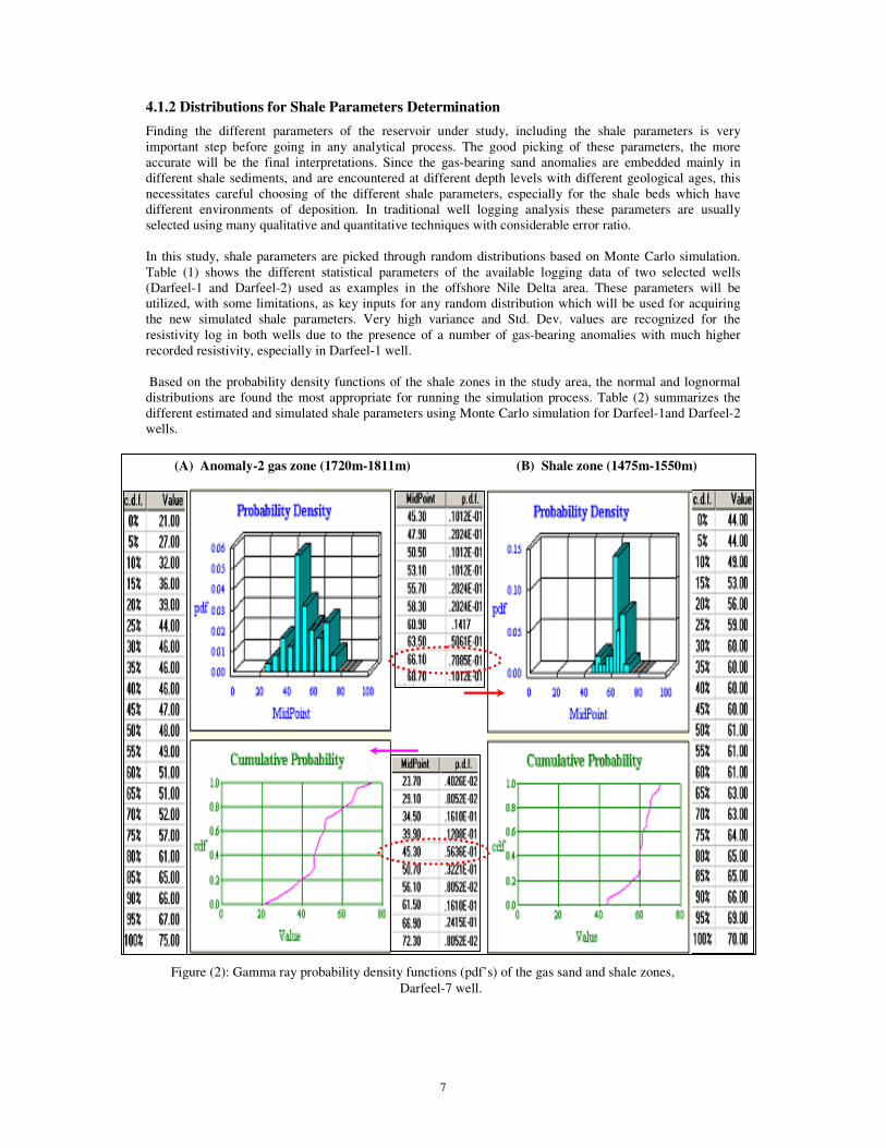
4.1.1 Probability Density Functions (PDF’s)

A number of probability density functions (pfd’s) are constructed for a number of wells in the area. The

study sections (Pliocene gas-bearing formations) are classified, in terms of shale content, into a number of

clean sand and shale entities or zones. Then, different types of pfd’s are constructed for each of these zones

separately. These functions are very important as it determine the type of the distribution and the best guess

of the parameters which will be further used in simulating certain petrophysical property. Figure 2 shows an

example of the constructed probability density functions (pfd’s) for the gas-bearing sand and shale zones in

Darfeel-7 well.

The figure gives best chance or highest probabilities of 0.56 and 0.71 with mid points of 45.30 and 66.10 for

the gamma ray log in the gas sand and shale zones, respectively.

Figure (1): Map showing the location

of the two studied areas.

7

4.1.2 Distributions for Shale Parameters Determination

Finding the different parameters of the reservoir under study, including the shale parameters is very

important step before going in any analytical process. The good picking of these parameters, the more

accurate will be the final interpretations. Since the gas-bearing sand anomalies are embedded mainly in

different shale sediments, and are encountered at different depth levels with different geological ages, this

necessitates careful choosing of the different shale parameters, especially for the shale beds which have

different environments of deposition. In traditional well logging analysis these parameters are usually

selected using many qualitative and quantitative techniques with considerable error ratio.

In this study, shale parameters are picked through random distributions based on Monte Carlo simulation.

Table (1) shows the different statistical parameters of the available logging data of two selected wells

(Darfeel-1 and Darfeel-2) used as examples in the offshore Nile Delta area. These parameters will be

utilized, with some limitations, as key inputs for any random distribution which will be used for acquiring

the new simulated shale parameters. Very high variance and Std. Dev. values are recognized for the

resistivity log in both wells due to the presence of a number of gas-bearing anomalies with much higher

recorded resistivity, especially in Darfeel-1 well.

Based on the probability density functions of the shale zones in the study area, the normal and lognormal

distributions are found the most appropriate for running the simulation process. Table (2) summarizes the

different estimated and simulated shale parameters using Monte Carlo simulation for Darfeel-1and Darfeel-2

wells.

(A) Anomaly-2 gas zone (1720m-1811m) (B) Shale zone (1475m-1550m)

Figure (2): Gamma ray probability density functions (pdf’s) of the gas sand and shale zones,

Darfeel-7 well.

8

Table (1): The average, variance and standard deviation parameters of the main

logs in Darfeel-1 and Darfeel-2 wells.

Table (2): Shale parameters estimated by normal logging and simulation methods,

Darfeel-1 and Darfeel-2 wells.

Well Model Parameter ∆∆∆∆Tsh ρρρρbsh φφφφNsh Rtsh GRmin GRmax

Logging Logsh 138.04 2.132 40.02 0.92 42.12 72.13

µ 139.82 2.141 41.9 0.89 40.36 75.94

σ2 313.29 0.004 69.14 0.05 14.98 27.77

St.Dev. 17.70 0.062 8.315 0.23 3.87 5.27

Darf

eel-

1

Monte

Carlo

Simulation

Logsh 140.53 2.122 42.46 0.96 39.93 75.29

Logging Logsh 142.11 2.114 41.05 0.95 41.21 65.24

µ 139.62 2.134 43.32 0.91 38.44 68.04

σ2 25.20 0.002 14.29 0.07 7.40 14.82

St.Dev. 5.02 0.048 3.78 0.26 2.72 3.85

Darf

eel-

2

Monte

Carlo

Simulation

Logsh 141.54 2.126 41.7 0.88 40.25 67.68

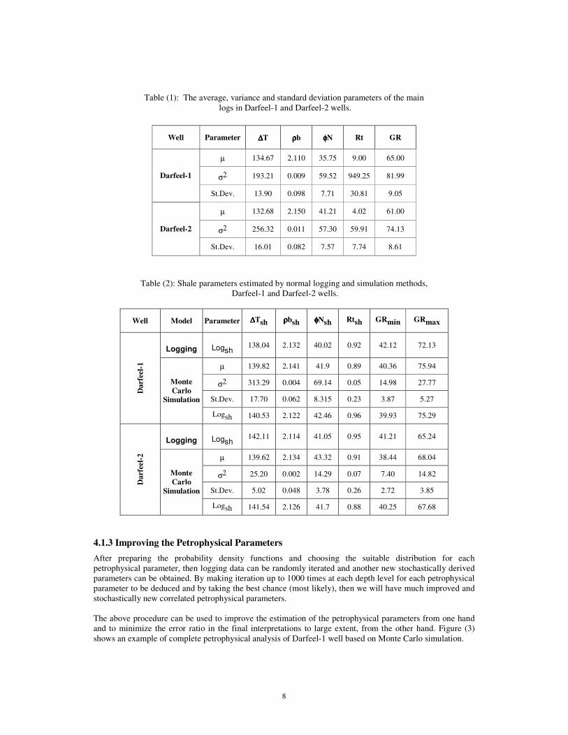
4.1.3 Improving the Petrophysical Parameters

After preparing the probability density functions and choosing the suitable distribution for each

petrophysical parameter, then logging data can be randomly iterated and another new stochastically derived

parameters can be obtained. By making iteration up to 1000 times at each depth level for each petrophysical

parameter to be deduced and by taking the best chance (most likely), then we will have much improved and

stochastically new correlated petrophysical parameters.

The above procedure can be used to improve the estimation of the petrophysical parameters from one hand

and to minimize the error ratio in the final interpretations to large extent, from the other hand. Figure (3)

shows an example of complete petrophysical analysis of Darfeel-1 well based on Monte Carlo simulation.

Well Parameter ∆∆∆∆T ρρρρb φφφφN Rt GR

µ 134.67 2.110 35.75 9.00 65.00

σ2 193.21 0.009 59.52 949.25 81.99 Darfeel-1

St.Dev. 13.90 0.098 7.71 30.81 9.05

µ 132.68 2.150 41.21 4.02 61.00

σ2 256.32 0.011 57.30 59.91 74.13 Darfeel-2

St.Dev. 16.01 0.082 7.57 7.74 8.61

9

Three gas-bearing sand levels are well detected (anomalies 2, 2-A and 3) at different depth levels, associated

with high apparent water resistivity. The petrophysical analysis of these levels show high effective porosity

(> 25%), high gas saturation (>50%) and low shale volume. Table (3) exhibits the normalized values for

the main petrophysical parameters of the detected gas-bearing anomalies using normal logging analyses and

simulation method. An effective range of differences can be observed between the results of both methods.

Figure (3): Petrophysical analysis of the Darfeel-1 well based on Monte Carlo simulation.

Table (3): Average petrophysical parameters of the gas-bearing anomalies

in Darfeel-1 well.

Method Zone Vsh Sw φeff

Anomaly 2 0.12 0.20 0.30

Anomaly 2-A 0.37 0.57 0.24 Monte Carlo

Simulation Anomaly 3 0.19 0.35 0.28

Anomaly 2 0.18 0.28 0.25

Anomaly 2-A 0.30 0.64 0.21 Normal Logging

Anomaly 3 0.24 0.39 0.24

10

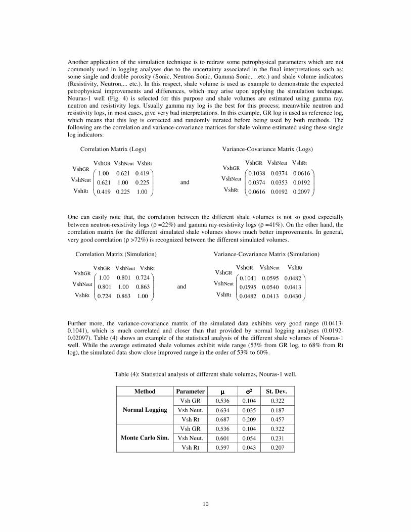
Another application of the simulation technique is to redraw some petrophysical parameters which are not

commonly used in logging analyses due to the uncertainty associated in the final interpretations such as;

some single and double porosity (Sonic, Neutron-Sonic, Gamma-Sonic,…etc.) and shale volume indicators

(Resistivity, Neutron,... etc.). In this respect, shale volume is used as example to demonstrate the expected

petrophysical improvements and differences, which may arise upon applying the simulation technique.

Nouras-1 well (Fig. 4) is selected for this purpose and shale volumes are estimated using gamma ray,

neutron and resistivity logs. Usually gamma ray log is the best for this process; meanwhile neutron and

resistivity logs, in most cases, give very bad interpretations. In this example, GR log is used as reference log,

which means that this log is corrected and randomly iterated before being used by both methods. The

following are the correlation and variance-covariance matrices for shale volume estimated using these single

log indicators:

Correlation Matrix (Logs) Variance-Covariance Matrix (Logs)

1.00 0.621 0.419

0.621 1.00 0.225

0.419 0.225 1.00

and

0.1038 0.0374 0.0616

0.0374 0.0353 0.0192

0.0616 0.0192 0.2097

One can easily note that, the correlation between the different shale volumes is not so good especially

between neutron-resistivity logs (ρ =22%) and gamma ray-resistivity logs (ρ =41%). On the other hand, the

correlation matrix for the different simulated shale volumes shows much better improvements. In general,

very good correlation (ρ >72%) is recognized between the different simulated volumes.

Correlation Matrix (Simulation) Variance-Covariance Matrix (Simulation)

1.00 0.801 0.724

0.801 1.00 0.863

0.724 0.863 1.00

and 0.1041 0.0595 0.0482

0.0595 0.0540 0.0413

0.0482 0.0413 0.0430

Further more, the variance-covariance matrix of the simulated data exhibits very good range (0.0413-

0.1041), which is much correlated and closer than that provided by normal logging analyses (0.0192-

0.02097). Table (4) shows an example of the statistical analysis of the different shale volumes of Nouras-1

well. While the average estimated shale volumes exhibit wide range (53% from GR log, to 68% from Rt

log), the simulated data show close improved range in the order of 53% to 60%.

Table (4): Statistical analysis of different shale volumes, Nouras-1 well.

Method Parameter µµµµ σσσσ2222 St. Dev.

Vsh GR 0.536 0.104 0.322

Vsh Neut. 0.634 0.035 0.187 Normal Logging

Vsh Rt 0.687 0.209 0.457

Vsh GR 0.536 0.104 0.322

Vsh Neut. 0.601 0.054 0.231 Monte Carlo Sim.

Vsh Rt 0.597 0.043 0.207

VshGR

VshNeut

VshRt

VshGR VshNeut VshRtVshGR

VshNeut

VshRt

VshGR VshNeut VshRt

VshGR

VshNeut

VshRt

VshGR VshNeut VshRt VshGR

VshNeut

VshRt

VshGR VshNeut VshRt

11

Figure (4): Shale volume analog of Nouras-1 well.

Figure (4) shows the shale volume analog for the different shale curves estimated by the logging (Track 3)

and simulation (Track 5) methods. Regarding track 3, very bad matching is observed between resistivity-

derived shale volume and other shale volumes estimated from neutron and gamma ray logs allover the entire

section of the well and between all of them especially in the upper and lower parts of the study section. This

is urged to the presence of low resistive clean sand bed in the upper part of the section (1108m-1185m)

which leads to high exaggerated shale volume as compared with other volumes derived from neutron and

gamma ray logs. Another reason is the presence of high resistive shale bed in the lower part of the section

(1940m-2045m), which could be interpreted by the resistivity log as clean bed with much reduced shale

volume. Track 5 on the hand, shows the simulated shale volumes. The matching between the resistivity-

derived shale volume and other estimated shale volumes (neutron and gamma ray) is remarkably improved

in the upper and lower parts of the study section and between all of them allover the entire section of the

well, in general.

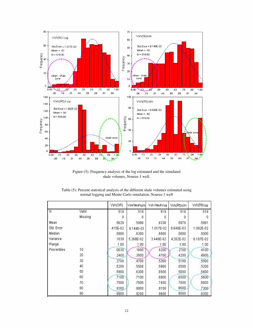
To clarify the differences between the two methods in a more detailed statistical way, frequency and percent

analyses are carried out upon the different concluded shale volumes. Figure (5) shows the frequency

crossplots of both log-derived and simulated data. The circular selections exhibit the low and high resistive

zones before and after simulation. Table (5), on the other hand, represents the percent statistical analysis of

the different shale volumes. It shows that the St. Error of the simulated parameters decreases remarkably.

Also, it appears clear that, although the normal logging methods ignoring the clean and shaly beds in case of

neutron (42%-47%) and resistivity logs (41%-48%), much more reliable values are given by the simulated

data; 16% to 38% and 27% to 42% for both logs, respectively. Furthermore, the low shale volume range

(56%-73%) given by the normal logging method (resistivity log) in front of the high resistive shale bed is

greatly treated after the simulation to a range of 65% to 86%, which is relatively close to that given by

gamma ray log (71% to 93%).

Low resistive

sand bed

High resistive

shale bed

12

Figure (5): Frequency analysis of the log estimated and the simulated

shale volumes, Nouras-1 well.

Table (5): Percent statistical analysis of the different shale volumes estimated using

normal logging and Monte Carlo simulation, Nouras-1 well

13

4.1.4 Predicting the Petrophysical Parameters

The for-mentioned simulation model can be used in predicting the missed sections of certain logs or even a

complete run of logs in an area. It can be also used for predicating the petrophysical parameters of a

proposed exploratory well providing that a satisfactory topological/geological neighbourhood constraint

(hard constraint) is completely well developed in the study area.

a. Constraints for Simulating New Well

A number of rules and constraints must be satisfied first before going to simulate new imaginary well in a

certain area. The most important of these are; 1) the well must be drilled in area with topological connected

sets, 2) good correlated petrophysical parameters between wells in the same connected set and the other set

in which a new well will be simulated, 3) the connected sets must attain the same structure elements and, 4)

the presence of the same lithological units (entities) as interpreted from seismic sections.

b. The Topological Connected Sets (Connected Space)

To simulate the petrophysical parameters of a new well in certain area, we have to make sure that the set

(area) of the new well is topologically connected with the other surrounding sets (areas), where many wells

are already drilled and their petrophysical parameters are interpreted and well known. So we have to define

the topological space and to find the relationships between the different sets in the study area based on

topological/geological rules.

c. Topological Space (X, ττττ)

If we suppose that the study area is the big universe set X which consists of many small sets Di, Dj,

Dk,….,Dn (Fig. 6). Then we have to check for an equivalence relationship (ρ) between the subsets to

construct the topology in X. In this respect we have three properties of ρ:

Reflexive: when Di ρ Di for all i = 1,2,3,….…….,n;

Symmetric: when Di ρ Dj & Dj ρ Di for all i = 1,2,3,………...,n;

Transitive: when Di ρ Dj & Dj ρ Dk & Di ρ Dk for all i = 1,2,3,………...,n;

The above properties between Di’s and Dj’s sets are achieved in case if the data of each set is reflexive to its

self (normal), or symmetrical if the same results can be obtained from the relation between two sets (Di ρ

Dj) by exchanging their positions (Dj ρ Di) and finally transitive if we have three sets and the relation

between the first and the second (Di ρ Dj) and the relation between the second and the third (Di ρ Dk) can

lead to the relation between the first and the third (Di ρ Dk).

After having the equivalence relationship between the subsets of X, then we have to construct the partitions

of X as follows:

[Di] = { Dj I Di ρ Dj} The cosets form the partition for X , where:

[ ] [ ] [ ]1

for all i jn

i

Di X and Di Dj φ=

= = ≠U I

These cosets construct a base for topology τ.

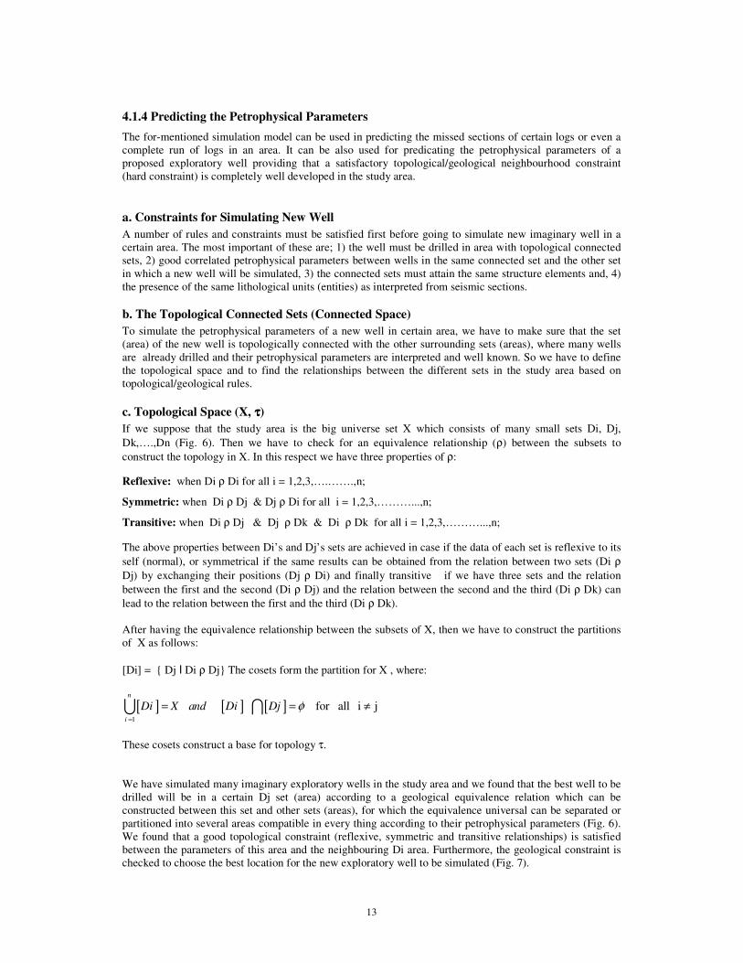
We have simulated many imaginary exploratory wells in the study area and we found that the best well to be

drilled will be in a certain Dj set (area) according to a geological equivalence relation which can be

constructed between this set and other sets (areas), for which the equivalence universal can be separated or

partitioned into several areas compatible in every thing according to their petrophysical parameters (Fig. 6).

We found that a good topological constraint (reflexive, symmetric and transitive relationships) is satisfied

between the parameters of this area and the neighbouring Di area. Furthermore, the geological constraint is

checked to choose the best location for the new exploratory well to be simulated (Fig. 7).

14

Figure (6): Off shore Nile Delta well base map showing the seismic lines,

the topological sets and location of the new well.

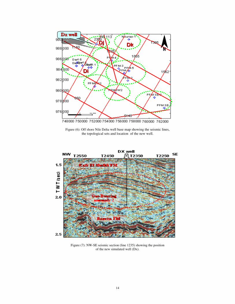
Figure (7): NW-SE seismic section (line 1235) showing the position

of the new simulated well (Dx).

15

From lateral seismic interpretations, we have to make sure that the section to be simulated contains the same

lithological entities for which the stochastic correlated parameters are already known. The new well (Dx) is

chosen at the intersection of seismic lines 1235 and 2300 at shot points 2380 and 1265 for both lines,

respectively. The expected two way time at the top of the gas-bearing anomaly in this well is 1.74 sec with

TVD depth of -1265m. The petrophysical parameters of the well are simulated using the available datasets

of the other wells in the Di set (Darfeel-1, Derfeel-2, Darfeel-7, etc), which have similar

neighbourhood/geological characters. The following is an example matrix of the different correlation

matrices, which can be produced for a certain petrophysical property (effective porosity) of the new well by

the simulation process:

1.00 0.95 0.92

0.95 1.00 0.90

0.92 0.90 1.00

Good correlation is observed between the predicted porosity of the new well (Dx) and the simulated

porosities of the other wells. The other different petrophysical parameters (Vsh, Sw, etc) are also simulated

using the same procedure. Table (6) summarizes the average simulated petrophysical parameters of the gas-

bearing anomaly-2 of the new well, relative to other wells in the study area.

Table (6): Average simulated petrophysical parameters of the gas anomaly-2

in Di and Dj sets.

Well Zone Vsh Sw φeff

Darfeel- 1 Anomaly 2 0.12 0.20 0.30

Darfeel- 2 Anomaly 2 0.17 0.35 0.25

Dx Anomaly 2 0.21 0.46 0.27

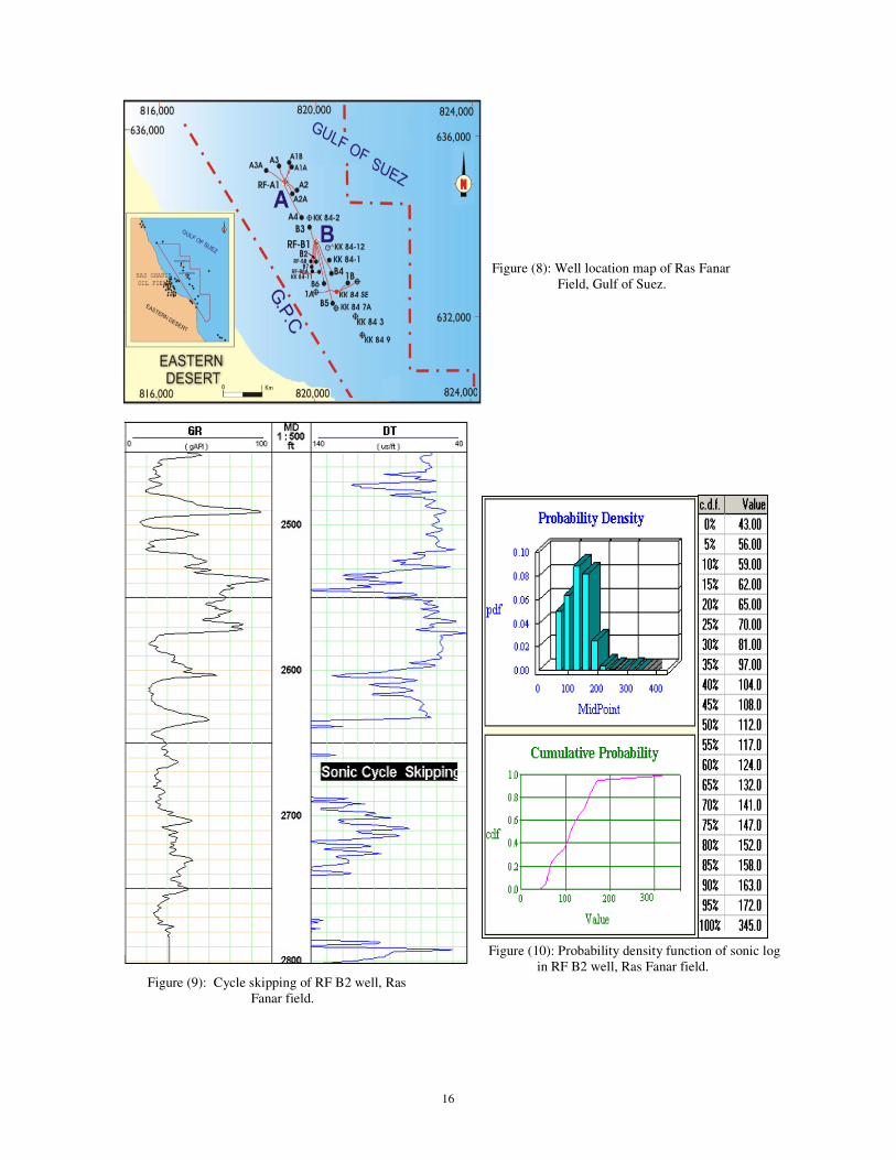
4.2 Case Study 2: Ras Fanar Field-Gulf of Suez

Ras Fanar area is located in the central part of the western margin of the Gulf of Suez about 3.5 km east of

Ras Gharib shoreline (Fig. 8). The field produces mainly from the Middle Miocene Nullipore carbonate

section which is deposited under shallow marine warm water conditions and is considered to be equivalent

to the Hammam Faraun Member of the Belayim Formation. Some problems concerning with the quality of

the sonic logging data are clearly noticed in this field due to the acoustic properties of the shallow carbonate

section.

Nullipore carbonate reservoir in Ras Fanar field is acoustically very soft especially in front of the more

porous intervals (∆T of +/- 190 µs/ft). This leads to low amplitude sonic signals and hence causes cycle

skipping problems in a number of sonic logs (Fig. 9).

Additionally, because the Nullipore is not well compacted (depth +/- 2000 to 3000 ftss) the usefulness of the

sonic log in logging and seismic interpretations is greatly limited. With the exception of the sonic tool,

almost the quality of other logs is generally good reflecting the borehole conditions. To overcome cycle

skipping problem and to make optimum use of the sonic log, a Monte Carlo-based simulation data are

derived for sonic logs in wells where the problem exist in correlation with the other sonic data of good

quality from surrounding wells. In this case study, RF B2 well is used to demonstrate how the simulation

procedure could be used to enhance and improve the acoustic properties of the Nullipore carbonates.

Figure (10) shows the probability density function of the sonic log for the carbonate section in RF B2 well.

It appears clear that the highest probability (best chance) for the sonic log is 0.04 with mid point of 158.9

Further more the shape of the density function assigns lognormal distribution for the simulation technique.

φeff Darf1

φeff Darf2

φeff Dx

φeff Darf1 φeff Darf2 φeff Dx

16

Figure (8): Well location map of Ras Fanar

Field, Gulf of Suez.

Figure (10): Probability density function of sonic log

in RF B2 well, Ras Fanar field.

Figure (9): Cycle skipping of RF B2 well, Ras

Fanar field.

17

A Monte Carlo simulation model is applied using the parameters concluded form the probability density

function and its distribution. Correlated stochastic parameters are constructed using the same procedure

followed in the first case study. Much more improvements are achieved for the sonic log especially in front

of the zone (2635ft-2790ft), which is greatly influenced by the cycle skipping (Fig. 11). To illustrate such

enhancements, a comparison is made between the correlation matrices of the used sonic data before and after

the simulation as follows:

Correlation Matrix (Logging) Correlation Matrix (MC Simulation)

1.00 0.91 0.65 0.92

0.91 1.00 0.87 0.95

0.65 0.87 1.00 0.72

0.92 0.95 0.72 1.00

1.00 0.95 0.87 0.94

0.95 1.00 0.91 0.98

0.87 0.91 1.00 0.92

0.94 0.98 0.92 1.00

Figure (11): Sonic log data of RF B2 well

before and after simulation.

∆TRF B3

∆TRF B8

∆TRF B2

∆TKK 84-1

∆TRF B3 ∆TRF B8 ∆TRF B2 ∆TKK 84-1

∆TRF B3

∆TRF B8

∆TRF B2

∆TKK 84-1

∆TRF B3 ∆TRF B8 ∆TRF B2 ∆TKK 84-1

18

The correlation matrix of the simulated parameters shows that sonic log data became much correlated with

other logs from the surrounding wells, especially between RF B2 well and both of RF B3 and KK 84-1

wells, where the correlation increases by percent more than 20%. Figure (11) exhibits the sonic log data of

RF B2 before and after simulation.

SUMMARY AND CONCLUSIONS

In this study both Monte Carlo and stochastic analyses are used as powerful tools for analyzing the

petrophysical parameters of the reservoirs in two different areas (offshore Nile Delta and Ras Fanar field).

The purpose of these analyses is mainly to improve the estimation of the petrophysical parameters from one

hand and to predict the petrophysical parameters of missed sections in old fields or even in new exploratory

areas, from the other hand.

Two types of constraints are defined before going on the simulation model. The first are hard constraints

based on number of probability density functions (pdf’s) for the different zones, fixed petrophysical-based

rules and known topological/geological relationship between the simulated wells. The second are the

simulation constraints, which are matter of change and deal mainly with some stochastic realizations of the

petrophysical parameters. Different types of statistical distributions and correlated multivariate variables

were used in the simulation, depending on the petrophysical property to be estimated. Also, a number of

correlation and variance-covariance matrices are constructed for the different logging data. The algorithm

begins with simulating correlated stochastic variables one by one by running a 100 times iteration in front of

each depth increment. By using rules based on the petrophysical information and by taking the best chance

(most likely), much improved and new stochastically correlated petrophysical parameters, will arise.

The simulation model is used to improve the estimation of the petrophysical parameters of reservoirs, which

are usually deduced by normal logging techniques. Due to the importance of shale parameters in the

evaluation of the gas-bearing reservoirs in the clastic offshore succession of the Nile Delta, these parameters

are chosen carefully using distributions based on Monte Carlo simulation.

Some petrophysical parameters which are not commonly used in logging interpretation due to the

uncertainty (shale volume indicators) are redrawn using the simulation model. The simulated Vsh values

are found more correlated and the errors in the interpretation which may arise by using normal logging

techniques due to certain rock physical properties (low resistive sand and

high resistive shale beds), are effectively reduced. Percent and frequency analyses are also used to compare

between the results of both methods. The other important petrophysical parameters, which are necessary for

evaluating the studied reservoirs, are all simulated and estimated using suitable Monte Carlo distributions.

Furthermore, the model is used to predicate the petrophysical parameters of a new proposed well (Dx) in the

offshore Nile Delta. To do that, the main area (X) is subdivided topologically into small areas (sets) Di, Dj,

Dk,….,Dn and a hard topological/geological neighbourhood constraint is examined first. An equivalence

relationship (ρ) between the subsets is studied to find the topological properties (reflexive, symmetric and

transitive) of the different sets based on geological/petrophysical rules. The different petrophysical

parameters of the new well (φ, Vsh, Sw, etc) are all simulated and predicted.

In Ras Fanar field, on the other hand, the model is used to solve the cycle skipping problem concerning with

sonic log, which is a common phenomenon in this field due to the acoustic properties of the carbonate

Nullipore reservoir. The quality of the simulated sonic data are greatly improved and show much more

correlation with other sonic data of good quality (ρ>87%).

The interpretations and results obtained form the simulation model are proved to be more accurate and

representative for the petrophysical properties of the studied reservoirs than that obtained form normal

logging analyses. So, this simulation model has a wide range of applicability and can be either used to

improve the estimation of the petrophysical parameters of the reservoirs and/or to make optimum use of the

available data in old fields or even in to predict the petrophysical parameters of wells in new exploratory

areas.

19

ACKNOWLEDGMENTS

The authors wish to thank the Egyptian General Petroleum Corporation, Petrobel Oil Company and Suez Oil

Company (SUCO) for providing the necessary data and facilities to accomplish this work. Special thanks go

to Mr. Fwazy Ibrahim and Mr. Sami Abd El Kader, petrophysics department, Suez Oil Company.

REFERENCES

Alabert, F. G., and Massonnat, G. J., (1990): Heterogeneity in a complex turbiditic reservoir: Stochastic

modeling of facies and petrophysical variability. Society of Petroleum Engineers Annual Technical

Conference and Exhibition, New Orleans, Louisiana, pp: 776- 790.

Bartlett, M. S. (1966): An introduction to stochastic processes, 2nd ed. Cambridge University Press,

Cambridge.

Bortoli, L. J., Alabert, F. G., Haas, A. G., and Journal, A. G., (1993): Constraining stochastic images to

seismic data, in Geostatistics Troia 92, 1, edited by Soares, A., Kluwer. Academic Publishers,

Dodrecht, Netherlands, pp: 325-337.

de Groot, P. F. M., Bril, A. H., Florist, F. J. T., and Campbell, A. E., (1996): Monte Carlo simulation of

wells. Geophysics, V. 61, No.3, pp: 631-638.

de Groot, P. F. M., Campbell, A. E., and Kavli, T., (1993): Seismic reservoir characterization using

artificial neural networks and stochastic modelling techniques: 55th Conf. Eur. Assn. Expl. Geophys.,

Stavanger, Expanded Abstracts, paper B047.

Deutsch, C. V., (2002): Geostatistical reservoir modelling. New York, Oxford University Press, 376p.

Fogg, G. E., Lucia, J. F., and Senger, R. K., (1991): Stochastic simulation of interwell scale heterogeneity

for improved prediction of sweep efficiency in a carbonate reservoir, in Reservoir Characterization II,

edited by Lake, L. W., Carroll, H. B., Jr., and Wesson, T. C., Academic Press Inc., Orlando,

Florida, pp: 487-544.

Haldorsen, H. H., and Chang, D. W., (1986): Notes on stochastic shales; from outcrop to simulation

model, in L. W. Lake and H. B. Caroll, eds., Reservoir characterization: London, Academic Press,

pp: 445- 48.

Haldorsen, H. H., and Damsleth, E., (1990): Stochastic modelling. Journal of Petroleum Technology, V.

42, No. 4, pp: 404-412.

Hearst, J. R, and Nelson, P. H., (1985): Well logging for physical properties. McGraw-Hill, N. Y., 189p.

Isaaks, E. H., and Srivastava, R. M., (1989): An introduction to applied geostatistics. Oxford University

Press, New York, 561p.

Law, A. M., and Kelton, W. D., (1991): Simulation modelling & Analysis. 2nd

ed. New York, McGraw

Hill, Inc.

Molz, F. J., and Boman, G. K., (1993): A fractal-based stochastic interpolation scheme in subsurface

hydrology. Water Resour. Res., V. 29, No.11, pp: 3769-3774.

Pyrcz, M. J., Catuneanu, O., and Deutsch, C. V., (2005): Stochastic surface-based modelling of

turbidite lobes. AAPG Bulletin, V. 89, No. 2, pp: 177-191.

Pyrcz, M. J., and Deutsch, C. V., (2003): Stochastic surface modelling in mud rich, fine-grained turbidite

lobes (abs.). AAPG Annual Meeting, May 11–14, Salt Lake City, Utah, Extended Abstract, 6p.

Rubinstein, R. Y. (1981): Simulation and the Monte Carlo method. New York, John Wiley & Sons.

Sambridge, M., and Mosegaard, K., (2002): Monte Carlo methods in geophysical inverse problems.

American Geophysical Union. Reviews of Geophysics, V. 40, No. 3, 29p.

Schlumberger Charts, (1991): Log interpretation charts. Schlumberger Educational Services. Houston,

Texas, U.S.A, 171p.

Strauss D. J., and Sadler, P. M., (1989): Stochastic models for the completeness of stratigraphic sections.

Math. Geol., 21, pp: 37-59.